Sub-Saharan Africa Transport Policy Program SSATP Working Paper No. 89-A

Version 2.0 - January 2009

User Guide

Rodrigo Archondo-Callao

SSATP Working Paper No. 89-A

Road Network Evaluation Tools

(RONET)

Version 2.0

User’s Guide

Rodrigo Archondo-Callao

January 2009

The SSATP is an international partnership to facilitate policy development and re-lated capacity building in the transport sector in Sub-Saharan Africa. Sound policies lead to safe, reliable and cost-effective transport, freeing people to lift themselves out of poverty, and helping countries to compete internationally.

The SSATP is a partnership of

35 SSA countries 8 Regional Economic Communities 3 African institutions UNECA, AU/NEPAD and AfDB 7 active donors

EC (main donor), Denmark, France, Ireland, Norway, Sweden and The World Bank (host)

Numerous public and private State and regional organizations

The SSATP gratefully acknowledges the financial contribution and support from the European Commission, the Governments of Denmark, France, Ire-land, Norway, Sweden, and The World Bank.

More publications on the SSATP website

www.worldbank.org/afr/ssatp

The World Bank and SSATP make no warranty in terms of correctness, accuracy, currentness, reliability, or oth-

erwise regarding the model. The user relies on the products of the software and the results solely at his or her own

risk. In no event will the World Bank or anyone else who has been involved in the creation of this product be liable

for its application or misapplication in the field. The World Bank reserves the right to make revisions and changes

from time to time without obligation to notify any person of such revisions and changes. Any views expressed in

this paper are those of the author and not necessarily of the sponsors.

v

Table of Contents

Preface .....................................................................................................................................................vii

Acknowledgments....................................................................................................................................ix

List of Acronyms and Abbreviations ......................................................................................................xi

Part A - Overview...................................................................................................................................... 1

Introduction ............................................................................................................................................. 1 Model Structure........................................................................................................................................ 4 Software Characteristics......................................................................................................................... 12

Part B – Current Condition Assessment Module ................................................................................. 17

Current Condition Assessment Overview ............................................................................................ 17 Basic Configuration................................................................................................................................ 17 Country Data .......................................................................................................................................... 23 Road Network Length ............................................................................................................................ 29 Length & Utilization............................................................................................................................... 31 Asset Value.............................................................................................................................................. 32 Roughness ............................................................................................................................................... 33 Network Distribution Charts................................................................................................................. 34 Network Monitoring Indicators ............................................................................................................ 34

Part C – Performance Assessment Module ........................................................................................... 37

Performance Assessment Overview....................................................................................................... 37 Standards Configuration........................................................................................................................ 41 Historical Expenditures.......................................................................................................................... 46 Network Performance............................................................................................................................ 46 Annual Work Program .......................................................................................................................... 48 Solution Catalog ..................................................................................................................................... 49 Road Works Distribution ...................................................................................................................... 49 Road Works Summary........................................................................................................................... 50 Historical Expenditures Comparison.................................................................................................... 50

Part D – Road User Revenues Module................................................................................................... 51

Road User Revenues Overview.............................................................................................................. 51 Vehicle Fleet Configuration................................................................................................................... 51 Road User Charges ................................................................................................................................. 52 Funding Requirements........................................................................................................................... 54 Fuel Consumption Revenues................................................................................................................. 56 Road User Revenues............................................................................................................................... 56 Requirements and Revenues Comparison............................................................................................ 57

vi

Annexes ................................................................................................................................................... 59

Annex 1: Paved Roads Roughness Progression Model ........................................................................ 59 Annex 2: Gravel Roads Gravel Loss Model ........................................................................................... 63 Annex 3: Road Works Effects ................................................................................................................ 64 Annex 4: Improvements to RONET Version 1.01................................................................................ 66

References ............................................................................................................................................... 69

vii

Preface

The Road Network Evaluation Tools (RONET) is a model which could be used by decision makers to

appreciate the current state of the road network, its relative importance to the economy (e.g. asset

value as percentage of GDP) and to compute a set of monitoring indicators to assess the performance

of the road network.

RONET assess the performance over time of the road network under different road maintenance stan-

dards. It determines, for example, the minimum cost for sustaining the network in its current condi-

tion and estimates the savings or the costs to the economy for maintaining the network at different

levels of service. RONET determines the allocation of expenditures among recurrent maintenance,

periodic maintenance, and rehabilitation road works.

This version of RONET determines the optimal maintenance standard for each road class (highest Net

Present Value) and compares it with the current (budget constraint) and other maintenance stan-

dards. Finally it determines the “funding gap,” defined as the difference between current maintenance

spending and required maintenance spending (to maintain the network at a given level of service), and

the effect of under spending on increased transport costs.

The new Road User Revenues Module, estimates the level of road user charges required (e.g. fuel levy)

to meet road maintenance expenditures under different budget scenarios. This could be used by road

fund boards to prepare a business case to negotiate and revise road tariffs on a sound basis.

RONET is developed from the same principles underlying the Highway Development and Manage-

ment Model (HDM-4). RONET uses simplified road user costs relationships, based on HDM-4 or

other relationships, and simplifies the road deterioration equations derived from the HDM-4 research.

Thus, RONET is a user friendly model which requires less data and less technical capacity to run than

HDM-4.

The primary audience of RONET is decision makers in the road sector, for whom it is designed as a

tool to advocate for continuous support for the road maintenance initiative.

Mustapha Benmaamar, Sr. Transport Specialist, SSATP

ix

Acknowledgments

The development of the RONET model is being funded by the Sub-Saharan Africa Transport Policy

Program (SSATP), which is a collaborative framework set up to improve transport policies and

strengthen institutional capacity in the Africa region. The model was developed by Rodrigo Ar-

chondo-Callao, Senior Highway Engineer, The World Bank, under the management of Olav E.

Ellevset, Sr. Transport Specialist, SSATP, and Mustapha Benmaamar, Sr. Transport Specialist, SSATP.

The model development is benefiting from contributions of a peer advisory group composed of David

Luyimbazi (Uganda), Godwin Brocke (Ghana), Atanásio Mugunhe (Mozambique), Joseph Lwiza

(Tanzania), Torben Larsen (Denmark), Eliamin Tenga (Tanzania), and Alberto Nogales (Bolivia).

xi

List of Acronyms and Abbreviations

AADT Average Annual Daily Traffic

ANE National Roads Administration in Mozambique

ESA Equivalent Standard Axles

ETWTR Energy, Transport & Water Department’s Transport Unit

(The World Bank)

GDP Gross Domestic Product

HDM Highway Development & Management

HNMS Highway Network Management System (Mozambique)

IQL Information Quality Level

IRI International Roughness Index

Km Kilometer

PAM Performance Assessment Model

PMORALG Prime Ministers Office Regional Administration and Local Government

PMS Pavement Management System

RAFU Road Agency Formation Unit

RAI Rural Access Indicator

RED Road Economic Decision Model

RMI Road Management Initiative

RMMS Road Maintenance Management System (Tanzania)

ROCKS Road Cost Knowledge System

RONET Road Network Evaluation Tools

RSSS Road Sector Strategy Study (Mozambique)

RUC Road User Charges Model

RUCKS Road User Costs Knowledge System

SAM Social Accounting Matrix

SSATP Sub-Saharan Africa Transport Policy Program

ST Surface Treatment

TANROADS Tanzania National Roads Agency

TTC Total Transport Costs

UNRA Uganda National Roads Authority

USD United States Dollar

VOC Vehicle operating cost

1

Part A - Overview

INTRODUCTION

The Road Network Evaluation Tools (RONET) model is being developed for the Sub-Saharan Africa

Transport Policy Program1 (SSATP) by the Energy, Transport and Water Department, Transport An-

chor (ETWTR), of the World Bank to assist decision makers to accomplish the following:

Monitor the current condition of the road network Plan allocation of resources Assess the consequences of macro-policies on the road network Evaluate road user charges revenues

RONET is a tool for assessing the performance of road maintenance and rehabilitation policies and

the importance of the road sector to the economy. This in turn demonstrates to stakeholders the im-

portance of continued support for road maintenance initiatives. It assesses the current network condi-

tion and traffic, computes the asset value of the network and road network monitoring indicators. It

uses country-specific relationships between maintenance spending and road condition, and between

road condition and road user costs, to assess the performance over time of the network under different

road works standards. It determines, for example, the minimum cost for sustaining the network in its

current condition. It also estimates the savings or the costs to the economy to be obtained from main-

taining the network at different levels of road condition. It further determines the proper allocation of

expenditures among recurrent maintenance, periodic maintenance, and rehabilitation road works.

Finally it determines the “funding gap,” defined as the difference between current maintenance spend-

ing and required maintenance spending (to maintain the network at a given level of road condition),

and the effect of under spending on increased transport costs.

The model is developed from the same principles underlying the accepted economic evaluation model

Highway Development and Management Model2 (HDM-4), adopting simplified road user costs rela-

tionships and simplified road deterioration equations derived from the HDM-4 research. HDM-4 is

an economic evaluation module of a Pavement Management System that can perform a strategic

evaluation of a network, evaluating a series of road classes similar to what is being done in RONET.

HDM-4 has comprehensive road deterioration and road user cost relationships, has great flexibility on

the way of defining the maintenance, rehabilitation or improvement standards to be evaluated, and

performs a budget constraint optimization. The characteristic of HDM-4 is that it has many input data

requirements, requires an HDM-4 specialist to run the model, and its output are limited and require

external manipulation. For example, very few of the RONET outputs are given by HDM-4 automati-

cally, but most of the RONET outputs can be obtained from an HDM-4 run after processing the

HDM-4 inputs and outputs in Excel or Access. The characteristic of RONET is the use of simplified

road deterioration and road user costs relationships, the restricted way defining the standards, the

2

inability to evaluate improvement standards, and the lack of a budget constraints optimization mod-

ule.

The primary audience for RONET is decision makers in the road sector, for whom it is designed as a

tool for advocacy of specific revenue enhancing or cost recovery measures. This new version of

RONET provides an interface between road maintenance expenditures and needs with the funding

requirements through road user charges. This could be used by road fund boards to develop a business

case to negotiate and revise road tariffs on a sound basis.

RONET is being developed for use in the Africa region, but there are no impediments to its applica-

tion in any other country worldwide. RONET includes a series of analytical tools designed to evaluate

the road network and road sector of a country at a macro-level by evaluating a series of representative

road classes, which can be characterized, for example, as (i) functional classification, (ii) surface type,

(iii) traffic level, (iv) road condition, (v) terrain, (vi) climate, and (vii) geographical region.

In the past SSATP has developed two other software tools, also designed to evaluate an entire road

network by evaluating a series of representative road classes, as follows:

The Road User Charges Model Version 3.03 (RUC), which evaluates scenarios of road user

charges in a country, evaluating road classes in good and fair condition differentiated by traf-

fic level, and estimates routine and periodic maintenance requirements derived from look-up

solution tables. The RUC model represents the entire network of a country by a maximum of

160 road classes that are functions of traffic, percent of cars, trucks loading, pavement

strength, environment, level of agency costs, and vehicle operating costs.

The Performance Assessment Model Version 1.04 (PAM), which estimates the performance

of a road network under different budget scenarios, evaluating road classes on any road con-

dition but not differentiating the road classes by traffic level, and estimates routine and peri-

odic maintenance requirements derived from a straight line deterioration model. The PAM

model represents the entire network of a country by a maximum of 64 road classes that are

functions of functional classification, pavement type, and condition.

RONET is being developed to replace the functionality of the RUC and PAM models and to add new

evaluation modules and output reports. RONET is being developed in a modular form, characterizes

the entire road network of a country by allowing the definition of a maximum of 625 road classes, and

includes simplified road deterioration models based on HDM-4 research. RONET version 2.0 imple-

ments the following evaluation modules:

Current Condition Assessment that calculates current road network statistics and network

monitoring indicators

Performance Assessment that evaluates the road network performance under different reha-

bilitation and maintenance budget scenarios and presents the consequences to the road

agency, the road user, and the road infrastructure

Road User Revenues that evaluates revenues being collected from road user charges and com-

pares them with the funding requirements

3

The main improvements of version 2.0 are the following:

New module to evaluate road user revenues was added

Current Condition Assessment Module now computes network safety indicators

Performance Assessment Module was redesigned to compare either (i) budget scenarios, (ii)

maintenance and rehabilitation standards scenarios, or (iii) custom standard scenarios

Performance Assessment Module now computes the optimal standard per road class (highest

Net Present Value) representing the optimal budget scenario

Performance Assessment Module has now new output reports presenting, for example, the

annual work program, solution catalog and affordability indicators for a given budget sce-

nario

Custom budget scenario is now user defined by selecting one maintenance standard per net-

work type and traffic level

RONET is now calculating the road works costs per Vehicle-Km ($/veh-km) for a given

budget scenario

The default network types are now Motorways, Primary, Secondary, Tertiary and Unclassi-

fied

4

MODEL STRUCTURE

To run RONET you first review the Configuration pages and modify any configuration data, if neces-

sary. Cells with a bright yellow background indicate country-specific inputs that you are expected to

modify, whereas cells with dim yellow backgrounds indicate user-defined RONET defaults that most

likely you will not need to modify. Then you enter the country-specific inputs at the following Input

Data pages:

Country Data that collects land area, total population, rural population, gross domestic prod-

uct at current prices, total Country road network, diesel and gasoline fuel consumption, total

vehicle fleet, discount rate, traffic growth rates, pavement widths, capital works unit costs, re-

current maintenance works unit costs, traffic level characteristics, vehicle fleet unit road user

costs relationship to roughness, and accidents rates and costs

Road Network Length that collects the road network length distribution by road classes that

are functions of network type, surface type, traffic category and condition category

Historical Expenditures that collects historical average road expenditures and road works dur-

ing the last five years per surface class and road work type

Road User Charges that collects current road user charges assigned to a road fund, main road

agency, other road sector, and general budget

Funding Requirements that collects the funding requirements for recurrent maintenance, pe-

riodic maintenance, rehabilitation, administration, and investment expenditures to be cover

by road user charges

The RONET road network length can cover the entire road network system of the country (roads,

highways, expressways, streets, avenues, and so forth), or a partial road network; for example, the road

network of a state or province of the country, or the road network managed by the main road agency.

The road network is represented by road classes that are a function of (i) five network types, (ii) five

surface types, (iii) five traffic categories, and (iv) five condition categories, which total a maximum of

625 road classes. Table 1 illustrates the representative road classes.

5

Table 1. Matrix of Road Classes: Overall Network Evaluation

Matrix of Road Classes: Overall Network Evaluation

Network Surface TypeType Concrete Asphalt S.T. Gravel EarthMotorwaysPrimarySecondaryTertiaryUnclassified

Traffic Condition CategoryCategory Very Good Good Fair Poor Very PoorTraffic ITraffic IITraffic IIITraffic IVTraffic V

Network Types

The road network is subdivided into as many as five network types that are user defined. The default

configuration subdivides the network into five network types characterized by functional classifica-

tion, but with the option to change the default configuration and redefine the characteristics of each

road network type. For example, each network type can represent a different, region, terrain type, or

climate type. Table 2 below shows the default configuration and sample user-defined configurations.

Table 2. Default Configuration and Alternative Configurations

Default Alternative

Configuration Configurations Examples

Network Types by Types by Types by

Type Functional Class Geographic Region Terrain Type

1 Motorways North Region Flat Terrain

2 Primary South Region Hilly Terrain

3 Secondary Easthern Region Mountainous Terrain

4 Tertiary Western Region NA

5 Unclassified Central Region NA

The default RONET road network types are based on the functional classification of the roads. The

default network types are as follows:

Motorways: Roads specially designed and built for motor traffic, which does not serve proper-

ties bordering on the roads, with four lanes or more lanes, separate carriageways for the two

directions of traffic, and with access control.

6

Primary: Arterial, main, trunk, or national roads, which are roads outside urban areas that

belong to the top-level road network and generally, have higher design standards than other

roads. These roads generally provide the highest level of mobility, at the highest speed, for

long interrupted traffic. These roads form the principal avenue of communication between

and through major regions of the country, between regional capitals and key towns that have

significant national economic and social interaction, and between the country and adjoining

countries, whose main function is to provide access to freight terminals, including ports.

Secondary: Collectors, classified as rural or regional roads, which are the main feeder routes

into primary roads, and provide the main links between primary roads. These roads generally

provide a lower degree of mobility than primary roads, being designed for travel at lower

speeds and for shorter distances. These roads form the principal avenue of communication

between primary roads and key towns and between primary roads and important centers,

which have a significant economic, social tourist, or recreation role (for example, tourism

and resource development).

Tertiary: Local roads, which are classified as rural or local roads. The roads are characterized

by a comparatively low-level design standard and traffic. These roads provide basic access be-

tween residential and commercial properties, connecting with higher-order roads. The func-

tion of these roads is to provide the only access to scattered rural settlements and primarily

serve local social services, as well as provide access to markets and generally form the first

phase of the journey for commuters.

Unclassified: Unclassified roads, which are roads that do not fall into any of the previous cate-

gories. These roads comprise special-purpose public roads that cannot be assigned to any

other class above, and which are provided almost exclusively for one specific activity or func-

tion, such as recreational, forestry, mining, national parks, or dam access.

On different countries, different road networks are managed by different road agencies or entities;

therefore, RONET allows for definition of the management responsibility type of each road network.

On the RONET Basic Configuration page, you assign one possible management type or entity (man-

agement and funding responsibility) to each road network type. The default user-defined management

types are the following:

Private sector: roads that are under the jurisdiction of concessionaires

National road agency: roads that are under the jurisdiction of the national road agency

Regional road agencies: roads that are under the jurisdiction of regional, provincial, or state

governments

Local road agencies: roads under the jurisdiction of district or local governments

Urban municipalities: roads, streets and avenues that are under the jurisdiction of city or

town governments.

Surface Types

Each network type is subdivided into the following five possible surface types:

Cement concrete pavement

Asphalt mix pavement

7

Surface treatment pavement

Gravel road

Earth road

The characteristics of each surface type are defined on the Basic Configuration page.

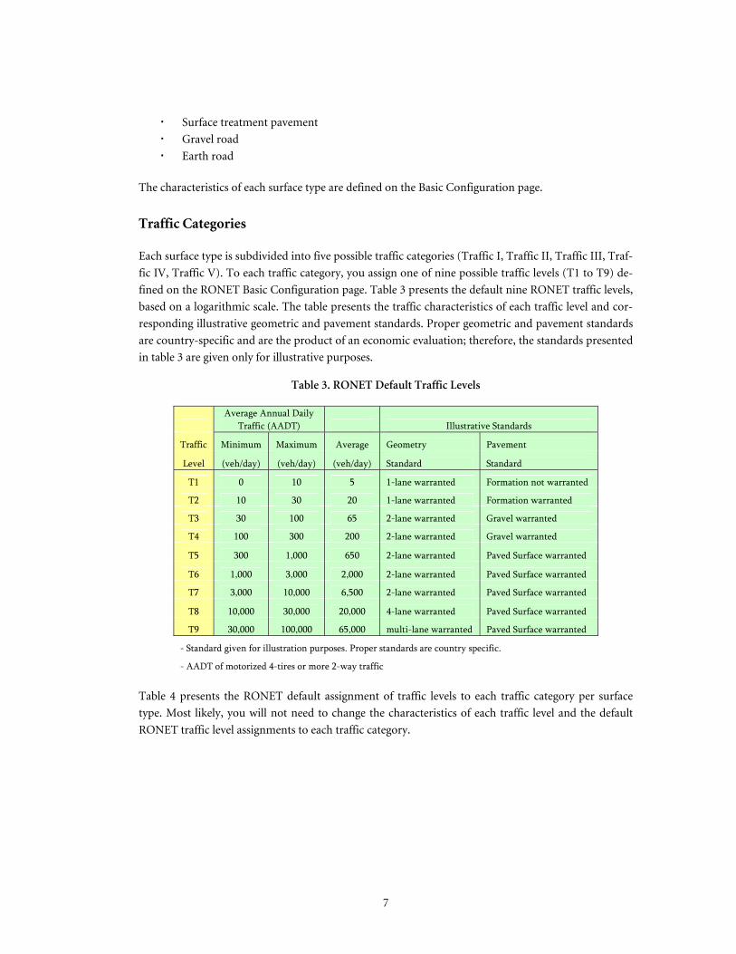
Traffic Categories

Each surface type is subdivided into five possible traffic categories (Traffic I, Traffic II, Traffic III, Traf-

fic IV, Traffic V). To each traffic category, you assign one of nine possible traffic levels (T1 to T9) de-

fined on the RONET Basic Configuration page. Table 3 presents the default nine RONET traffic levels,

based on a logarithmic scale. The table presents the traffic characteristics of each traffic level and cor-

responding illustrative geometric and pavement standards. Proper geometric and pavement standards

are country-specific and are the product of an economic evaluation; therefore, the standards presented

in table 3 are given only for illustrative purposes.

Table 3. RONET Default Traffic Levels

Average Annual Daily

Traffic (AADT) Illustrative Standards

Traffic Minimum Maximum Average Geometry Pavement

Level (veh/day) (veh/day) (veh/day) Standard Standard

T1 0 10 5 1-lane warranted Formation not warranted

T2 10 30 20 1-lane warranted Formation warranted

T3 30 100 65 2-lane warranted Gravel warranted

T4 100 300 200 2-lane warranted Gravel warranted

T5 300 1,000 650 2-lane warranted Paved Surface warranted

T6 1,000 3,000 2,000 2-lane warranted Paved Surface warranted

T7 3,000 10,000 6,500 2-lane warranted Paved Surface warranted

T8 10,000 30,000 20,000 4-lane warranted Paved Surface warranted

T9 30,000 100,000 65,000 multi-lane warranted Paved Surface warranted

- Standard given for illustration purposes. Proper standards are country specific.

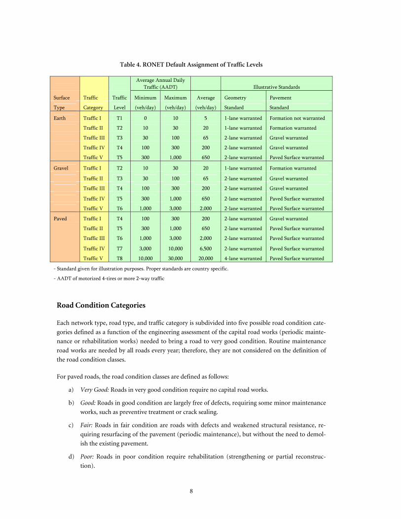
- AADT of motorized 4-tires or more 2-way traffic Table 4 presents the RONET default assignment of traffic levels to each traffic category per surface

type. Most likely, you will not need to change the characteristics of each traffic level and the default

RONET traffic level assignments to each traffic category.

8

Table 4. RONET Default Assignment of Traffic Levels

Average Annual Daily

Traffic (AADT) Illustrative Standards

Surface Traffic Traffic Minimum Maximum Average Geometry Pavement

Type Category Level (veh/day) (veh/day) (veh/day) Standard Standard

Earth Traffic I T1 0 10 5 1-lane warranted Formation not warranted

Traffic II T2 10 30 20 1-lane warranted Formation warranted

Traffic III T3 30 100 65 2-lane warranted Gravel warranted

Traffic IV T4 100 300 200 2-lane warranted Gravel warranted

Traffic V T5 300 1,000 650 2-lane warranted Paved Surface warranted

Gravel Traffic I T2 10 30 20 1-lane warranted Formation warranted

Traffic II T3 30 100 65 2-lane warranted Gravel warranted

Traffic III T4 100 300 200 2-lane warranted Gravel warranted

Traffic IV T5 300 1,000 650 2-lane warranted Paved Surface warranted

Traffic V T6 1,000 3,000 2,000 2-lane warranted Paved Surface warranted

Paved Traffic I T4 100 300 200 2-lane warranted Gravel warranted

Traffic II T5 300 1,000 650 2-lane warranted Paved Surface warranted

Traffic III T6 1,000 3,000 2,000 2-lane warranted Paved Surface warranted

Traffic IV T7 3,000 10,000 6,500 2-lane warranted Paved Surface warranted

Traffic V T8 10,000 30,000 20,000 4-lane warranted Paved Surface warranted

- Standard given for illustration purposes. Proper standards are country specific.

- AADT of motorized 4-tires or more 2-way traffic

Road Condition Categories

Each network type, road type, and traffic category is subdivided into five possible road condition cate-

gories defined as a function of the engineering assessment of the capital road works (periodic mainte-

nance or rehabilitation works) needed to bring a road to very good condition. Routine maintenance

road works are needed by all roads every year; therefore, they are not considered on the definition of

the road condition classes.

For paved roads, the road condition classes are defined as follows:

a) Very Good: Roads in very good condition require no capital road works.

b) Good: Roads in good condition are largely free of defects, requiring some minor maintenance

works, such as preventive treatment or crack sealing.

c) Fair: Roads in fair condition are roads with defects and weakened structural resistance, re-

quiring resurfacing of the pavement (periodic maintenance), but without the need to demol-

ish the existing pavement.

d) Poor: Roads in poor condition require rehabilitation (strengthening or partial reconstruc-

tion).

9

e) Very Poor: Roads in very poor condition require full reconstruction, almost equivalent to new

construction.

For gravel roads, the road condition classes are defined as follows:

a) Very Good: Roads in very good condition require no capital road works.

b) Good: Roads in good condition are roads that require only spot regraveling.

c) Fair: Roads in fair condition require regraveling (periodic maintenance).

d) Poor: Roads in poor condition require partial reconstruction.

e) Very Poor: Roads in very poor condition require full reconstruction, almost equivalent to new

construction.

For earth roads, the road condition classes are defined as follows:

a) Very Good: Roads in very good condition require no capital road works.

b) Good: Roads in good condition are roads that require only spot repairs.

c) Fair: Roads in fair condition require heavy grading (periodic maintenance).

d) Poor: Roads in poor condition require partial reconstruction.

e) Very Poor: Roads in very poor condition require full reconstruction, almost equivalent to new

construction.

Table 5 presents a summary of the capital road works needed to bring a road to very good condition

by surface type.

Table 5. Capital Road Works Needed to Bring a Road to Very Good Condition

Capital Road Works Needed to Bring a Road to Very Good Condition

Condition

Category Bituminous Roads Gravel Roads Earth Roads

Very Good None None None

Good Preventive Treatment Spot Regraveling Spot Repairs

Fair Resurfacing Regraveling Heavy Grading

Poor Strengthening Partial Reconstruction Partial Reconstruction

Very Poor Full Reconstruction Full Reconstruction Full Reconstruction Figure 1 presents the road condition categories of bituminous roads, taking into account the area of

cracking and the pavement age.

10

Figure 1. Road Condition Categories of Bituminous Roads

0

10

20

30

40

50

60

70

80

90

100

0 2 4 6 8 10 12 14 16 18 20

Year

Crac

king

Are

a (%

)

Very GoodGood

Fair

Poor

Very Poor

To assess the consequences to the road agency, the infrastructure, and the economy of applying differ-

ent maintenance and rehabilitation standards, RONET needs to associate an average roughness value

to each road condition category. Table 6 presents the default RONET basic characteristics of each road

condition class in terms of roughness and the corresponding car speeds on a flat terrain for unpaved

roads. The roughness values are country-specific and user-defined at the RONET Basic Configuration

page. Note that the car speeds are given for illustrative purposes and are not being used by the RONET

model.

RONET is by default configured to reflect average road characteristics that are applicable to Develop-

ing Countries conditions. If needed, RONET can be configured to reflect better local conditions. On

the configuration pages, cells with bright yellow backgrounds indicate country-specific inputs that you

are expected to modify, whereas cells with dim yellow background indicate user-defined RONET de-

faults that most likely you will not modify.

11

Table 6. Default RONET Basic Characteristics of Each Road Condition Class

Surface Condition Roughness (IRI m/km) Speeds

Type Category Minimum Maximum Average (km/hr)

Cement Very Good 1.0 2.5 2.0

Concrete Good 2.5 3.5 3.0

Fair 3.5 6.0 4.0

Poor 6.0 10.0 8.0

Very Poor 10.0 16.0 12.0

Asphalt Very Good 1.0 2.5 2.0

Mix Good 2.5 3.5 3.0

Fair 3.5 5.5 4.5

Poor 5.5 10.5 8.0

Very Poor 10.5 16.0 12.0

Surface Very Good 1.0 3.5 3.0

Treatment Good 3.5 4.5 4.0

Fair 4.5 6.5 5.5

Poor 6.5 11.5 9.0

Very Poor 11.5 16.0 13.0

Gravel Roads Very Good 1.0 6.0 5.0 90-110

Good 6.0 9.0 7.0 70-90

Fair 9.0 13.5 11.0 40-70

Poor 13.5 18.0 16.0 30-40

Very Poor 18.0 25.0 20.0 20-30

Earth Roads Very Good 1.0 8.0 7.0 90-110

Good 8.0 11.0 9.0 70-90

Fair 11.0 15.5 13.0 40-70

Poor 15.5 20.0 18.0 30-40

Very Poor 20.0 25.0 22.0 20-30

Speeds represent range of car speeds at the dry season on a flat terrain

12

SOFTWARE CHARACTERISTICS

RONET is implemented on a Microsoft Office Excel 2003 workbook. To run RONET, open the fol-

lowing Excel workbook:

RONET v2.00-MainModule-2009-01.xls RONET relies on Excel macros to perform its calculations; therefore, Excel has to be configured to

enable Excel macros. If Excel is properly configured, you will get the following message when opening

the RONET Excel workbook.

In this case, select the option “Enable Macros” to go to the RONET main menu.

If Excel is not properly configured, you will get the following message when opening the RONET Excel

workbook, indicating that the Excel security level is set to high.

13

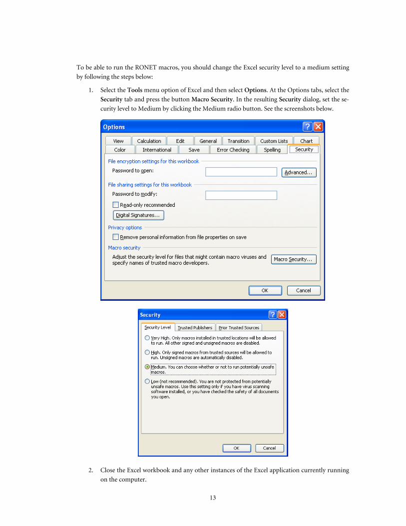
To be able to run the RONET macros, you should change the Excel security level to a medium setting

by following the steps below:

1. Select the Tools menu option of Excel and then select Options. At the Options tabs, select the

Security tab and press the button Macro Security. In the resulting Security dialog, set the se-

curity level to Medium by clicking the Medium radio button. See the screenshots below.

2. Close the Excel workbook and any other instances of the Excel application currently running

on the computer.

14

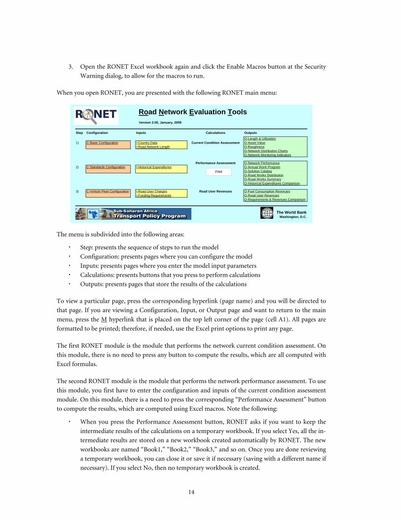
3. Open the RONET Excel workbook again and click the Enable Macros button at the Security

Warning dialog, to allow for the macros to run. When you open RONET, you are presented with the following RONET main menu:

Road Network Evaluation Tools Version 2.00, January, 2009

Step Configuration Inputs Calculations Outputs

O-Length & Utilization1) C-Basic Configuration I-Country Data Current Condition Assessment O-Asset Value

I-Road Network Length O-RoughnessO-Network Distribution ChartsO-Network Monitoring Indicators

Performance Assessment O-Network Performance2) C-Standards Configuration I-Historical Expenditures O-Annual Work Program

O-Solution CatalogO-Road Works DistributionO-Road Works SummaryO-Historical Expenditures Comparison

3) C-Vehicle Fleet Configuration I-Road User Charges Road User Revenues O-Fuel Consumption RevenuesI-Funding Requirements O-Road User Revenues

O-Requirements & Revenues Comparison

The World BankWashington, D.C.

PAM

The menu is subdivided into the following areas:

Step: presents the sequence of steps to run the model

Configuration: presents pages where you can configure the model

Inputs: presents pages where you enter the model input parameters

Calculations: presents buttons that you press to perform calculations

Outputs: presents pages that store the results of the calculations To view a particular page, press the corresponding hyperlink (page name) and you will be directed to

that page. If you are viewing a Configuration, Input, or Output page and want to return to the main

menu, press the M hyperlink that is placed on the top left corner of the page (cell A1). All pages are

formatted to be printed; therefore, if needed, use the Excel print options to print any page.

The first RONET module is the module that performs the network current condition assessment. On

this module, there is no need to press any button to compute the results, which are all computed with

Excel formulas.

The second RONET module is the module that performs the network performance assessment. To use

this module, you first have to enter the configuration and inputs of the current condition assessment

module. On this module, there is a need to press the corresponding “Performance Assessment” button

to compute the results, which are computed using Excel macros. Note the following:

When you press the Performance Assessment button, RONET asks if you want to keep the

intermediate results of the calculations on a temporary workbook. If you select Yes, all the in-

termediate results are stored on a new workbook created automatically by RONET. The new

workbooks are named “Book1,” “Book2,” “Book3,” and so on. Once you are done reviewing

a temporary workbook, you can close it or save it if necessary (saving with a different name if

necessary). If you select No, then no temporary workbook is created.

15

To compute the results takes between two and five minutes, depending on the computer

processing speed. The status of the calculations is presented on the Excel status line at the

bottom left corner of the screen. When all the calculations are done, the model presents a

message indicating the end of the calculations and the duration of the calculations.

The third RONET module is the module that computes the revenues collected from road user charges

and compares them with the financing needs. To use this module, you first have to enter the configu-

ration and inputs of the current condition assessment and performance assessment modules and exe-

cute the “Performance Assessment” button of the performance assessment module. On the road user

revenues module, there is no need to press any button to compute the results, which are all computed

with Excel formulas.

When you are displaying a Configuration, Input, or Output page, you will notice that some cells have

a yellow background. These cells with the yellow backgrounds are input cells where you enter your

input data or your model output choices. Cells with bright yellow backgrounds indicate country-

specific inputs that you are expected to modify, whereas cells with dim yellow backgrounds indicate

user-defined RONET defaults that most likely you will not need to modify. All the cells with a white

background contain labels (black font) or formulas (blue font). You are only allowed to edit the input

cells with yellow backgrounds because all other cells are protected. If you need to unprotect a page,

select the Tools menu option of Excel, and then select Protection and Unprotect Sheet.

RONET can be used with any currency, but the numerical fields and decimal places are set up to fit

U.S. dollars and all RONET default values are provided in U.S. dollars. If you decide to use any other

currency, you have to be careful to enter all the inputs and default values using the same currency on

all RONET configuration and input pages. In that case, all the results will be presented in that cur-

rency.

To carry out a current condition assessment, follow the steps below.

If necessary, modify the basic configuration

Enter the country data

Enter the network data

View and the corresponding output pages

To carry out a performance assessment, follow the steps below.

If necessary, modify the basic configuration, if you had not done that before

If necessary, modify the standards configuration

Enter the country data, if you had not done that before

Enter the network data, if you had not done that before

Optionally, enter the historical expenditures data

Press the “Performance Assessment” button and wait for the calculations to be completed

View and the corresponding output pages, selecting on row 1 a corresponding budget sce-

nario,, network surface class, road work type, or period

To carry out a road user revenues evaluation, follow the steps below.

Carry out a current condition assessment and a performance assessment

16

If necessary, modify the vehicle fleet configuration

Enter the road user charges data

Enter the funding requirements data

View and the corresponding output pages

17

Part B – Current Condition Assessment Module

CURRENT CONDITION ASSESSMENT OVERVIEW

This RONET module evaluates the current network condition and presents summary network statis-

tics and network monitoring indicators. The outputs of this module are the following.

Length & Utilization: presents the network length and network utilization distribution by

network type and surface type

Asset Value: presents the network maximum asset value and network current asset value dis-

tribution by network type and surface type

Roughness: presents the average network roughness weighted by km and the average network

roughness weighted by vehicle-km by network type and surface type

Network Distribution Charts: presents network distribution charts of the network length,

utilization, and maximum and current asset value by network type and surface type

Network Monitoring Indicators: presents road network monitoring indicators

All the results are computed using Excel formulas; therefore, there is no button to press to compute

the results which are recomputed automatically when you change any configuration data or input

data. The Output pages contain tables and charts and are formatted to be printed; therefore, if neces-

sary, use the Excel print options to print these pages.

BASIC CONFIGURATION

Management Types

On the Basic Configuration page, the first option is to define the possible management responsibility

types present in the country. RONET shows, as one of its outputs, the required road agency costs and

other indicators summarized by these management types. The default management types are given

below:

Private sector: roads that are under the jurisdiction of concessionaires

National road agency: roads that are under the jurisdiction of the national road agency

Regional road agencies: roads that are under the jurisdiction of regional, provincial or

state governments

Local road agencies: roads under the jurisdiction of district or local governments

Urban municipalities: roads, streets and avenues that are under the jurisdiction of city or

town governments

18

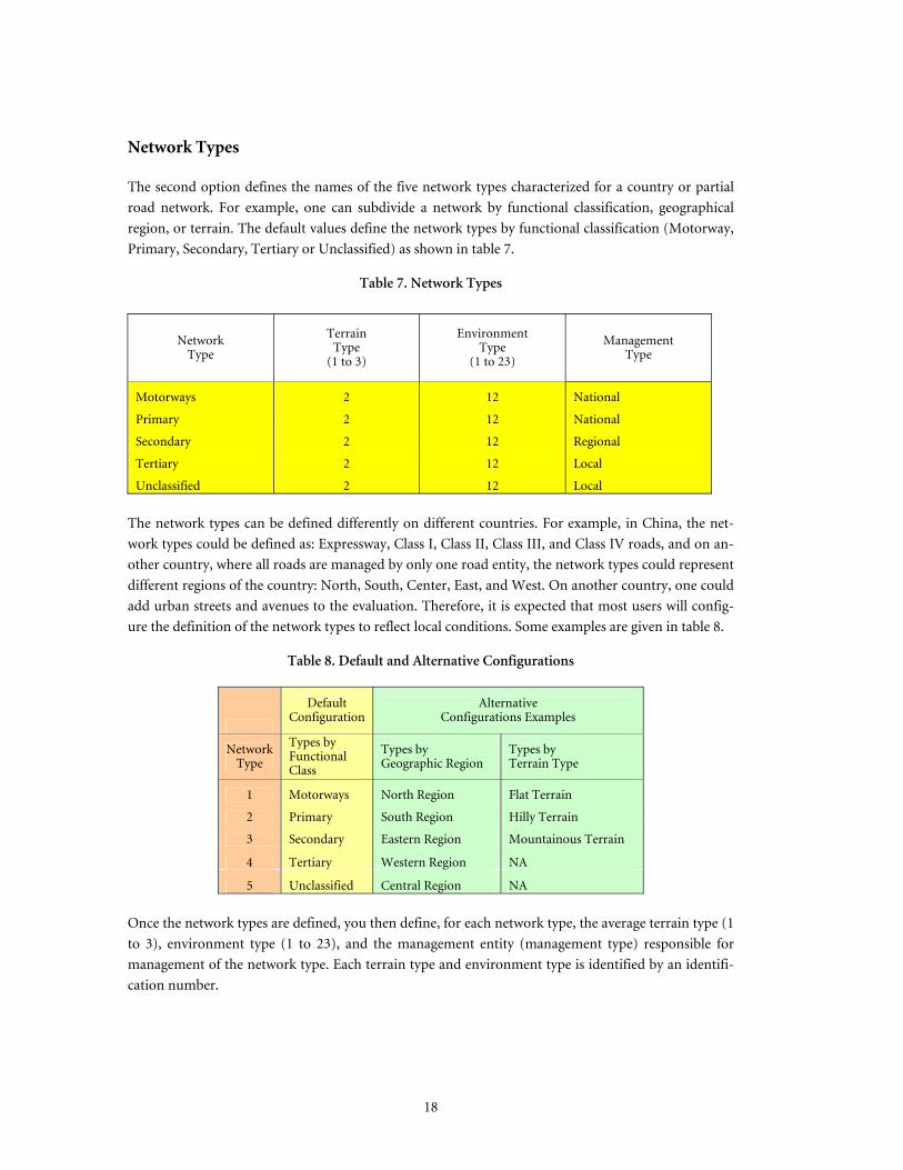
Network Types

The second option defines the names of the five network types characterized for a country or partial

road network. For example, one can subdivide a network by functional classification, geographical

region, or terrain. The default values define the network types by functional classification (Motorway,

Primary, Secondary, Tertiary or Unclassified) as shown in table 7.

Table 7. Network Types

Network Type

Terrain Type

(1 to 3)

Environment Type

(1 to 23)

Management Type

Motorways 2 12 National

Primary 2 12 National

Secondary 2 12 Regional

Tertiary 2 12 Local

Unclassified 2 12 Local The network types can be defined differently on different countries. For example, in China, the net-

work types could be defined as: Expressway, Class I, Class II, Class III, and Class IV roads, and on an-

other country, where all roads are managed by only one road entity, the network types could represent

different regions of the country: North, South, Center, East, and West. On another country, one could

add urban streets and avenues to the evaluation. Therefore, it is expected that most users will config-

ure the definition of the network types to reflect local conditions. Some examples are given in table 8.

Table 8. Default and Alternative Configurations

Default Configuration

Alternative Configurations Examples

Network Type

Types by Functional Class

Types by Geographic Region

Types by Terrain Type

1 Motorways North Region Flat Terrain

2 Primary South Region Hilly Terrain

3 Secondary Eastern Region Mountainous Terrain

4 Tertiary Western Region NA

5 Unclassified Central Region NA Once the network types are defined, you then define, for each network type, the average terrain type (1

to 3), environment type (1 to 23), and the management entity (management type) responsible for

management of the network type. Each terrain type and environment type is identified by an identifi-

cation number.

19

Terrain Types

The average physical characteristics of the three possible terrain types (1-flat, 2-hilly or 3-

mountainous) vary by country; therefore, they are defined at the Basic Configuration page. Here you

enter the corresponding average Rise & Fall, in m/km, and Horizontal Curvature, in degrees/km, of

each terrain type, following the HDM-4 definitions of Rise & Fall and Horizontal Curvature. The de-

fault RONET values given in table 9 are based on worldwide averages. It is expected that you will ad-

just these values to reflect local conditions only if local data are readily available on existing HDM-4

studies.

Table 9. Terrain Types

Terrain Type

(1 to 3) Terrain

Classification

Rise & Fall

(m/km)

Horizontal Curvature (deg/km)

1 Flat 0 0

2 Hilly 40 100

3 Mountainous 80 300

Environmental Types

The Basic Configuration page allows for the definition of 23 possible environment types defined by

function of the moisture and temperature classification. Here you can enter, for each environment

type, the average rainfall, in mm/month, and the HDM-4 environment coefficient of road deteriora-

tion for paved roads. The default values are given below in Table 10. It is expected that very few users

will modify the environmental coefficients of road deterioration for paved roads. These coefficients

can only be adjusted after a detailed calibration of the HDM-4 road deterioration equations, which

typically is not readily available.

20

Table 10. Environment Types

Environment Type

(1 to 23)

Moisture Classification

Temperature Classification

Rainfall (mm/month)

Environment Coefficient

(#)

1 Arid Tropical 15 0.005

2 Arid Sub-tropical Hot 15 0.100

3 Arid Sub-tropical Cool 15 0.015

4 Arid Temperate Cool 15 0.025

5 Arid Temperate Freeze 15 0.040

6 Semi-arid Tropical 50 0.010

7 Semi-arid Sub-tropical Hot 50 0.015

8 Semi-arid Sub-tropical Cool 50 0.025

9 Semi-arid Temperate Cool 50 0.035

10 Semi-arid Temperate Freeze 50 0.060

11 Sub-humid Tropical 100 0.020

12 Sub-humid Sub-tropical Hot 100 0.025

13 Sub-humid Sub-tropical Cool 100 0.040

14 Sub-humid Temperate Cool 100 0.060

15 Sub-humid Temperate Freeze 100 0.100

16 Humid Tropical 175 0.025

17 Humid Sub-tropical Hot 175 0.030

18 Humid Sub-tropical Cool 175 0.060

19 Humid Temperate Cool 175 0.100

20 Humid Temperate Freeze 175 0.200

21 Per-humid Tropical 210 0.030

22 Per-humid Sub-tropical Hot 210 0.040

23 Per-humid Sub-tropical Cool 210 0.070

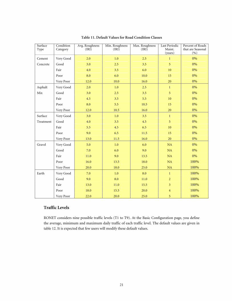
Road Condition Classes

The next Basic Configuration page option is to define (per surface type) for each of the five road con-

dition categories (Very Good, Good, Fair, Poor and Very Poor), the roughness characteristics (aver-

age, minimum, and maximum), the number of years since the last periodic maintenance or rehabilita-

tion road work, and the estimate of the percent of roads that are seasonal. The default values are given

in table 11. It is expected that few users will modify the default roughness values and the years since

the last periodic maintenance or rehabilitation road work. Users in other regions might adjust these

values to reflect local conditions. Users might want to adjust the percent of roads that are seasonal,

which is a rough estimate of the percent of the road in each road condition class that are not all-

weather roads, because this is a country-specific input.

21

Table 11. Default Values for Road Condition Classes

Surface Type

Condition Category

Avg. Roughness (IRI)

Min. Roughness (IRI)

Max. Roughness (IRI)

Last Periodic Maint. (years)

Percent of Roads that are Seasonal

(%)

Cement Very Good 2.0 1.0 2.5 1 0%

Concrete Good 3.0 2.5 3.5 5 0%

Fair 4.0 3.5 6.0 10 0%

Poor 8.0 6.0 10.0 15 0%

Very Poor 12.0 10.0 16.0 20 0%

Asphalt Very Good 2.0 1.0 2.5 1 0%

Mix Good 3.0 2.5 3.5 5 0%

Fair 4.5 3.5 5.5 10 0%

Poor 8.0 5.5 10.5 15 0%

Very Poor 12.0 10.5 16.0 20 0%

Surface Very Good 3.0 1.0 3.5 1 0%

Treatment Good 4.0 3.5 4.5 5 0%

Fair 5.5 4.5 6.5 10 0%

Poor 9.0 6.5 11.5 15 0%

Very Poor 13.0 11.5 16.0 20 0%

Gravel Very Good 5.0 1.0 6.0 NA 0%

Good 7.0 6.0 9.0 NA 0%

Fair 11.0 9.0 13.5 NA 0%

Poor 16.0 13.5 18.0 NA 100%

Very Poor 20.0 18.0 25.0 NA 100%

Earth Very Good 7.0 1.0 8.0 1 100%

Good 9.0 8.0 11.0 2 100%

Fair 13.0 11.0 15.5 3 100%

Poor 18.0 15.5 20.0 4 100%

Very Poor 22.0 20.0 25.0 5 100%

Traffic Levels

RONET considers nine possible traffic levels (T1 to T9). At the Basic Configuration page, you define

the average, minimum and maximum daily traffic of each traffic level. The default values are given in

table 12. It is expected that few users will modify these default values.

22

Table 12. Default Values for Traffic Levels

Traffic Avg. Traffic Min. Traffic Max. Traffic

Level (AADT) (AADT) (AADT)

T1 5 0 10

T2 20 10 30

T3 65 30 100

T4 200 100 300

T5 650 300 1,000

T6 2,000 1,000 3,000

T7 6,500 3,000 10,000

T8 20,000 10,000 30,000

T9 65,000 30,000 100,000

Traffic Categories

Finally, you define the traffic level that is associated to each of the five traffic category (Traffic I, Traffic

II, Traffic III, Traffic IV, and Traffic V), per surface type, and the structural number of each traffic

category for paved roads. The structural number represents the modified structural number at the

time of construction or last rehabilitation of the road, computed as defined on the HDM-III7 docu-

mentation, equal to the structural number computed following American Association of State High-

way & Transportation Officials (AASHTO) guidelines, plus adding the strength contribution of sub-

grade. The default values are given in table 13. It is expected that very few users will modify these de-

fault traffic levels per traffic category.

23

Table 13. Default Values for Traffic Categories

Surface Type

Traffic Category

Traffic Level (T1 to T9)

Avg. Traffic (AADT)

Min. Traffic (AADT)

Max. Traffic (AADT)

Structural Number for Paved Roads (#)

Cement Traffic I T4 200 100 300 6.0

Concrete Traffic II T5 650 300 1000 6.0

Traffic III T6 2000 1000 3000 6.0

Traffic IV T7 6500 3000 10000 6.0

Traffic V T8 20000 10000 30000 8.0

Asphalt Traffic I T4 200 100 300 1.5

Mix Traffic II T5 650 300 1000 2.0

Traffic III T6 2000 1000 3000 3.0

Traffic IV T7 6500 3000 10000 5.0

Traffic V T8 20000 10000 30000 8.0

Surface Traffic I T4 200 100 300 1.5

Treatment Traffic II T5 650 300 1000 2.0

Traffic III T6 2000 1000 3000 3.0

Traffic IV T7 6500 3000 10000 5.0

Traffic V T8 20000 10000 30000 8.0

Gravel Traffic I T2 20 10 30 NA

Traffic II T3 65 30 100 NA

Traffic III T4 200 100 300 NA

Traffic IV T5 650 300 1000 NA

Traffic V T6 2000 1000 3000 NA

Earth Traffic I T1 5 0 10 NA

Traffic II T2 20 10 30 NA

Traffic III T3 65 30 100 NA

Traffic IV T4 200 100 300 NA

Traffic V T5 650 300 1000 NA

COUNTRY DATA

On this page you enter the basic country data that is composed of the following elements:

Name and Year

Basic Characteristics

Traffic Growth Rate

Capital Road Works Unit Costs

Recurrent Maintenance Works Unit Costs

Traffic Levels Characteristics

Vehicle Fleet Unit road User Costs Relationship to Roughness

Accident Rates

Accident Costs

24

Name and Year

Here you enter the name of the country, or the name of the region of the country or road agency being

evaluated. RONET is set up to evaluate an entire road network of a country, but in some circum-

stances RONET can be used to evaluate only a region of a country; for example, a state or a province

of a country or a partial network managed by a road agency. Here you also enter the year of the road

network data and basic country characteristics. The year is entered for reference purposes; it is not

used in the calculations.

Basic Characteristics

At this table, you enter the country figures that are used to compute network monitoring indicators, as

well as by the network performance assessment and road revenues modules:

Land area (sq km): a country’s total area, excluding areas under inland bodies of water and

some coastal waterways

Total population (million persons): the mid-year estimates of all residents regardless of legal

status or citizenship

Rural population (million persons): the mid-year population of areas defined as rural in each

country and reported to the United Nations

GDP at current prices ($ billion): the gross domestic product at current prices that is the sum

of the gross value added by all resident producers in the economy, plus any product taxes and

minus any subsidies not included in the value of the products

Vehicle fleet (vehicles): the total number of road motor vehicles in use at the given year in the

country

Total road network length (km): the total road network length of the country

Total paved roads network length (km): the total paved roads network length of the country

Diesel roads consumption (million liters/year): the total annual diesel consumption in the

road sector

Gasoline roads consumption (million liters/year): the total annual gasoline consumption in

the road sector

Total accidents fatalities (persons/year): the total accident fatalities registered on the country

Total accidents serious injuries (persons/year): the total accidents serious injuries registered

on the country.

Discount rate (%): the planning discount rate adopted by the country, which is typically 12%

in developing countries.

The first four of these indicators can be found at the following World Bank website page:

http://go.worldbank.org/45B5H20NV0

Traffic Growth Rate

25

You define the expected annual traffic growth rate over the 20-year evaluation period for each network

type.

Capital Road Works Unit Costs

On RONET, the road agency road works are classified in the following manner:

Capital Road Works

- Periodic Maintenance

- Rehabilitation

- New Construction

Recurrent Maintenance Works

- Annual Works On and Outside de Carriageway

Here you enter the financial unit costs of the capital road works defined for each surface type, in $ per

km for a two-lane road. RONET works with two-lane equivalent road classes. The possible capital

road works, which are a function of the current road condition and network type, are shown in table

14.

Strengthening and reconstruction of paved roads and partial reconstruction, or full reconstruction of

unpaved roads are considered as rehabilitation works. The road works applied to roads in good and

fair condition are considered periodic maintenance works.

The RONET default values for basic characteristics and for traffic growth rate are for a fictitious

country; therefore, you must change them to reflect local conditions.

26

Table 14. Possible Capital Road Works

Surface Current Condition Road Work Type Road Work Class

Cement

Concrete

Good Condition

Fair Condition

Poor Condition

Very Poor Condition

No Road

Preventive Treatment

Resurfacing (Overlay)

Strengthening (Overlay)

Reconstruction

New Construction

Periodic Maintenance

Periodic Maintenance

Rehabilitation

Rehabilitation

New Construction

Asphalt

Mix

Good Condition

Fair Condition

Poor Condition

Very Poor Condition

No Road

Preventive Treatment

Resurfacing (Overlay)

Strengthening (Overlay)

Reconstruction

New Construction

Periodic Maintenance

Periodic Maintenance

Rehabilitation

Rehabilitation

New Construction

Surface

Treatment

Good Condition

Fair Condition

Poor Condition

Very Poor Condition

No Road

Preventive Treatment

Resurfacing (Reseal)

Strengthening (Overlay)

Reconstruction

New Construction

Periodic Maintenance

Periodic Maintenance

Rehabilitation

Rehabilitation

New Construction

Gravel

Roads

Good Condition

Fair Condition

Poor Condition

Very Poor Condition

No Road

Spot Regraveling

Regraveling

Partial Reconstruction

Full Reconstruction

New Construction

Periodic Maintenance

Periodic Maintenance

Rehabilitation

Rehabilitation

New Construction

Earth Roads

Good Condition

Fair Condition

Poor Condition

Very Poor Condition

No Road

Spot Repairs

Heavy Grading

Partial Reconstruction

Full Reconstruction

New Construction

Periodic Maintenance

Periodic Maintenance

Rehabilitation

Rehabilitation

New Construction

The unit costs of the capital works could vary by network type (different functional classification or

different region of the country), for example, because of different design standards; therefore, if neces-

sary, you can enter different values by network type. Here you also need to define the basic character-

istics of the regraveling, resurfacing, strengthening, and reconstruction options in terms of surface

layer thickness for regraveling, resurfacing, and strengthening, and resulting modified structural num-

ber and roughness for reconstruction.

The default values are given in table 15. It is expected that you will modify these default values to re-

flect local conditions. The default values reflect broadly developing countries conditions and were

derived by evaluating the World Bank’s Road Costs Knowledge System5 (ROCKS) that stores and

evaluates information on road works unit costs worldwide, and can be download at the following

World Bank Website:

http://worldbank.org/roadsoftwaretools/

27

Table 15. Default Values in Capital Road Works Unit Costs Capital Road Works Unit Costs

Two-Lane Unit Costs of Road Works ($/km) Thickness ReconstructionSurface Type Current Condition Road Work Class Road Work Type Motorways Primary Secondary Tertiary Unclassified (mm) Structural No. Roughness (IRI)Cement Concrete Good Condition Periodic Maintenance Preventive Treatment 12,000 12,000 12,000 8,571 8,571

Fair Condition Resurfacing (Overlay) 100,000 100,000 100,000 71,429 71,429 50Poor Condition Rehabilitation Strengthening (Overlay) 200,000 200,000 200,000 142,857 142,857 100Very Poor Condition Reconstruction 330,000 330,000 330,000 235,714 235,714 3 2.0No Road New Construction New Construction 400,000 400,000 400,000 285,714 285,714

Asphalt Mix Good Condition Periodic Maintenance Preventive Treatment 12,000 12,000 12,000 8,571 8,571Fair Condition Resurfacing (Overlay) 100,000 100,000 100,000 71,429 71,429 50Poor Condition Rehabilitation Strengthening (Overlay) 200,000 200,000 200,000 142,857 142,857 100Very Poor Condition Reconstruction 330,000 330,000 330,000 235,714 235,714 3 2.0No Road New Construction New Construction 400,000 400,000 400,000 285,714 285,714

Surface Treatment Good Condition Periodic Maintenance Preventive Treatment 12,000 12,000 12,000 8,571 8,571Fair Condition Resurfacing (Reseal) 27,000 27,000 27,000 19,286 19,286 12Poor Condition Rehabilitation Strengthening (Overlay) 160,000 160,000 160,000 114,286 114,286 80Very Poor Condition Reconstruction 260,000 260,000 260,000 185,714 185,714 2 2.5No Road New Construction New Construction 330,000 330,000 330,000 235,714 235,714

Gravel Good Condition Periodic Maintenance Spot Regravelling 3,000 3,000 3,000 2,143 2,143Fair Condition Regravelling 17,000 17,000 17,000 12,143 12,143 150Poor Condition Rehabilitation Partial Reconstruction 40,000 40,000 40,000 28,571 28,571Very Poor Condition Full Reconstruction 60,000 60,000 60,000 42,857 42,857No Road New Construction New Construction 80,000 80,000 80,000 57,143 57,143

Earth Good Condition Periodic Maintenance Spot Repairs 200 200 200 143 143Fair Condition Heavy Grading 800 800 800 571 571Poor Condition Rehabilitation Partial Reconstruction 8,000 8,000 8,000 5,714 5,714Very Poor Condition Full Reconstruction 25,000 25,000 25,000 17,857 17,857No Road New Construction New Construction 40,000 40,000 40,000 28,571 28,571

Recurrent Road Works Unit Costs

Here you enter the financial unit costs of the recurrent road works for each surface type, in $ per km

per year for a two-lane road. The recurrent road works unit costs vary by current road condition and

network type; therefore, if necessary, you can enter different values by road condition and network

type. Here you enter the total recurrent costs that are the sum of the annual road works done on the

carriageway (for example, grading, pothole patching, and so forth), and the annual road works done

outside the carriageway (for example, shoulder repairs, grass mowing, and so forth). The default val-

ues, which reflect broadly developing country conditions, are given in table 16. It is expected that you

will modify these default values to reflect local conditions.

Table 16. Default Values for Recurrent Maintenance Works Unit Costs

Traffic Levels Characteristics

On the Basic Configuration page, nine possible traffic levels (T1 to T9) are defined by characterizing

their average, minimum, and maximum Average Annual Daily Traffic (AADT). Here you define the

average traffic composition of each traffic level and define for each vehicle type: (i) the equivalent stan-

dard axles (ESA per vehicle), (ii) the average cargo payload per vehicle (tons per vehicle), and (iii) the

Recurrent Maintenance Works Unit CostsTwo-Lane Unit Costs of Road Works ($/km-year)

Surface Type Road Condition Road Work Class Road Work Type Motorways Primary Secondary Tertiary UnclassifiedCement Concrete Very Good Recurrent Maintenance Recurrent Maintenance 2,000 2,000 2,000 1,000 1,000

Good Recurrent Maintenance 2,500 2,500 2,500 1,250 1,250Fair Recurrent Maintenance 3,000 3,000 3,000 1,500 1,500Poor Recurrent Maintenance 1,500 1,500 1,500 750 750Very Poor Recurrent Maintenance 1,500 1,500 1,500 750 750

Asphalt Mix Very Good Recurrent Maintenance Recurrent Maintenance 2,000 2,000 2,000 1,000 1,000Good Recurrent Maintenance 2,500 2,500 2,500 1,250 1,250Fair Recurrent Maintenance 3,000 3,000 3,000 1,500 1,500Poor Recurrent Maintenance 1,500 1,500 1,500 750 750Very Poor Recurrent Maintenance 1,500 1,500 1,500 750 750

Surface Treatment Very Good Recurrent Maintenance Recurrent Maintenance 2,000 2,000 2,000 1,000 1,000Good Recurrent Maintenance 2,500 2,500 2,500 1,250 1,250Fair Recurrent Maintenance 3,000 3,000 3,000 1,500 1,500Poor Recurrent Maintenance 1,500 1,500 1,500 750 750Very Poor Recurrent Maintenance 1,500 1,500 1,500 750 750

Gravel Very Good Recurrent Maintenance Recurrent Maintenance 1,000 1,000 1,000 500 500Good Recurrent Maintenance 1,250 1,250 1,250 626 626Fair Recurrent Maintenance 1,500 1,500 1,500 750 750Poor Recurrent Maintenance 750 750 750 375 375Very Poor Recurrent Maintenance 750 750 750 375 375

Earth Very Good Recurrent Maintenance Recurrent Maintenance 300 300 300 150 150Good Recurrent Maintenance 450 450 450 225 225Fair Recurrent Maintenance 600 600 600 300 300Poor Recurrent Maintenance 300 300 300 150 150Very Poor Recurrent Maintenance 300 300 300 150 150

28

average number of passengers per vehicle (passengers per vehicle). Based on this information, RONET

computes for each traffic level: (i) the total equivalent standard axles per year, in million ESA per year,

(ii) the average cargo payload per vehicle, in tons per vehicle, and (iii) the average number of passen-

gers per vehicle, in passengers per vehicle. The ESA loading is used to compute the road deterioration

of paved roads and the average payload and passengers per vehicle are used to compute the network

monitoring indicators: annual freight carried over road network (annual ton-km) and annual passen-

gers carried over road network (annual passenger-km).

The default values, which reflect broadly developing country conditions, are given in table 17. It is

expected that you will calibrate these default values to reflect local conditions.

Table 17. Default Values for Traffic Levels Characteristics

Traffic Level T1 T2 T3 T4 T5 T6 T7 T8 T9

Average Annual Daily Traffic (AADT) = 5 20 65 200 650 2,000 6,500 20,000 65,000Vehicle Equivalent Standard Axles Cargo Payload Passengers Typical Traffic Composition (%)Type (ESA/vehicle) (Tons/vehicle) ersons/vehic (%) (%) (%) (%) (%) (%) (%) (%) (%)Motorcycle 0.00 0.20 1 0.0% 0.0% 0.0% 0.0% 0.0% 0.0% 0.0% 0.0% 0.0%Car Small 0.00 0.10 2 0.0% 0.0% 0.0% 0.0% 0.0% 0.0% 0.0% 0.0% 0.0%Car Medium 0.00 0.30 2 24.4% 24.4% 24.4% 24.4% 29.8% 29.8% 29.8% 34.1% 34.1%Delivery Vehicle 0.01 0.90 2 33.3% 33.3% 33.3% 33.3% 27.2% 27.2% 27.2% 26.8% 26.8%Four-Wheel Drive 0.02 0.80 2 0.0% 0.0% 0.0% 0.0% 0.0% 0.0% 0.0% 0.0% 0.0%Truck Light 0.10 2.40 1 8.9% 8.9% 8.9% 8.9% 6.7% 6.7% 6.7% 4.5% 4.5%Truck Medium 1.25 5.70 1 10.5% 10.5% 10.5% 10.5% 7.8% 7.8% 7.8% 4.9% 4.9%Truck Heavy 2.28 10.60 1 3.3% 3.3% 3.3% 3.3% 3.4% 3.4% 3.4% 2.5% 2.5%Truck Articulated 4.63 22.30 1 2.7% 2.7% 2.7% 2.7% 4.5% 4.5% 4.5% 3.0% 3.0%Bus Light 0.04 1.25 12 10.6% 10.6% 10.6% 10.6% 15.0% 15.0% 15.0% 16.4% 16.4%Bus Medium 0.70 2.50 30 3.2% 3.2% 3.2% 3.2% 2.8% 2.8% 2.8% 3.9% 3.9%Bus Heavy 0.80 3.20 40 3.2% 3.2% 3.2% 3.2% 2.8% 2.8% 2.8% 3.9% 3.9%

Total = 100.0% 100.0% 100.0% 100.0% 100.0% 100.0% 100.0% 100.0% 100.0%ESA Loading (M ESA/year) = 0.000 0.000 0.000 0.000 0.000 0.000 0.000 0.000 0.000

Payload/Vehicle (tons/vehicle) = 0.00 0.00 0.00 0.00 0.00 0.00 0.00 0.00 0.00Passengers/Vehicle (persons/vehicle) = 0.00 0.00 0.00 0.00 0.00 0.00 0.00 0.00 0.00

Vehicle Fleet Unit Road User Costs Relationship to Roughness

RONET computes the network road user costs for different maintenance and rehabilitation standards

at the performance assessment module. Road user costs are a function of road roughness; therefore,

there is a need to define the relationship between unit road user costs and roughness for a particular

country. On RONET, this relationship takes the form of the following cubic polynomial.

Unit Road User Costs ($/vehicle-km) = a0 + a1*IRI + a2*IRI^2 + a3*IRI^3

Where “Unit Road User Costs” represents the unit road use costs of the vehicle fleet, “IRI” is the

roughness of the road, in IRI, m/km, and a0, a1, a2 and a3 are coefficients of the cubic polynomial.

Here you need to define the coefficients of the cubic polynomial for each traffic level based on local

conditions. To compute these coefficients effortlessly, you can use the World Bank’s Road User Costs

Knowledge System (RUCKS)6 version 1.2 that contains an Excel model designed for this purpose, and

presents representative vehicle fleet characteristics for different regions of the World. RUCKS can be

downloaded at the following World Bank Website:

http://worldbank.org/roadsoftwaretools/.

29

When you compute unit user costs with RUCKS or with any other model, you compute either finan-

cial (market costs) or economic (without taxes and subsidies) road user costs. RONET compares road

agency and road user in financial terms to simplify the evaluation compared with the HDM-4 model

that compares economic costs, because most of the time HDM-4 users adopt the same conversion

factor to road agency costs and road user costs; therefore, there is a RONET input factor that repre-

sents the factor to multiply the defined unit road user costs computed by the cubic polynomials to

convert them to financial costs. If the cubic polynomials are already computing financial costs then the

multiplier factor is 1.0. The default values, which reflect broadly developing country conditions, are

given below in table 18. It is expected that you will modify these default values to reflect local condi-

tions.

Table 18. Vehicle Fleet Unit Road User Costs Default Values

Traffic Level T1 T2 T3 T4 T5 T6 T7 T8 T9Average Annual Daily Traffic (AADT) 5 20 65 200 650 2,000 6,500 20,000 65,000

a0 coefficient 0.27966 0.27966 0.27966 0.27966 0.28871 0.28871 0.28840 0.27267 0.41310a1 coefficient -0.00028 -0.00028 -0.00028 -0.00028 -0.00055 -0.00055 -0.00060 -0.00222 0.00613a2 coefficient 0.00144 0.00144 0.00144 0.00144 0.00148 0.00148 0.00151 0.00173 0.00049a3 coefficient -0.00003 -0.00003 -0.00003 -0.00003 -0.00003 -0.00003 -0.00003 -0.00004 -0.00002

1.00Factor to multiply defined unit road user costs above to convert them to

Unit Road User Costs ($/veh-km) = a0 + a1*IRI + a2*IRI^2 + a3*IRI^3

Accident Rates and Accident Costs

RONET estimates the total annual fatalities and serious injuries due to road accidents in the road net-

work based on average fatalities and serious injuries rates (number per 100 million vehicle-km) per

surface type. To compute the road safety costs, (i) you enter a multiplier to the GDP per capita defined

to obtain the costs of a fatality to society, with suggested range 60 to 80 as given by the International

Road Assessment Programme (iRAP) publication: The True Cost of Road Crashes 8, and (ii) you enter

the serious injury costs as a percentage of the fatality cost, with suggested range 20% to 30%. The de-

fault values, which reflect broadly developing countries conditions, are given below in table 19.

Table 19. Accident Rates and Costs

Accident Rates Motorways Primary Secondary Tertiary UnclassifiedFatalities accident rate (number of fatalities per 100 million vehicle-km) 10 10 10 10 10Serious injuries accident rate (number of serious injuries per 100 million vehicle-km) 100 100 100 100 100

Acciddent CostsFactor to multiply GDP per capita to obtain fatality cost 70 Fatalities accident cost ($) 64,400Serious injuries cost as a percent of fatality cost 25% Serious injuries accident cost ($) 16,100

ROAD NETWORK LENGTH

On this page you enter the network length distribution by network type, surface type, traffic category,

and road condition category. You should enter the two-lane equivalent network length belonging to

each road class, in kilometers. That means if there is a four- lane road, you should enter the corre-

sponding two-lane equivalent length, which is twice the length of the four-lane road. If there are no

kilometers on the network represented by a road class, you can enter zero kilometers or leave the cell

blank. Figure 2 presents the structure of this page.

30

Figure 2. Road Network Length Default Values (Country XYZ) Road Network Two-Lane Equivalent Length (km)

Primary PrimarySurface Treatment Gravel

Condition (IRI) Very Good Good Fair Poor Very Poor Condition (IRI) Very Good Good Fair Poor Very PoorTraffic (AADT) 3 4 5.5 9 13 Total Traffic (AADT) 5 7 11 16 20 TotalTraffic I <300 0.0 0.0 0.0 0.0 0.0 0.0 Traffic I <30 0.0 0.0 0.0 49.0 292.0 341.0Traffic II 300-1000 0.0 51.0 36.0 62.0 26.0 175.0 Traffic II 30-100 0.0 5.0 11.0 7.0 179.0 202.0Traffic III 1000-3000 4.0 13.0 67.0 88.0 32.0 204.0 Traffic III 100-300 0.0 0.0 0.0 0.0 0.0 0.0Traffic IV 3000-10000 0.0 0.0 0.0 0.0 0.0 0.0 Traffic IV 300-1000 0.0 0.0 0.0 0.0 0.0 0.0Traffic V >10000 0.0 0.0 0.0 0.0 0.0 0.0 Traffic V >1000 0.0 0.0 0.0 0.0 0.0 0.0Total 4.0 64.0 103.0 150.0 58.0 379.0 Total 0.0 5.0 11.0 56.0 471.0 543.0

Secondary SecondarySurface Treatment Gravel

Condition (IRI) Very Good Good Fair Poor Very Poor Condition (IRI) Very Good Good Fair Poor Very PoorTraffic (AADT) 3 4 5.5 9 13 Total Traffic (AADT) 5 7 11 16 20 TotalTraffic I <300 0.0 0.0 10.0 0.0 0.0 10.0 Traffic I <30 7.0 56.0 393.0 631.0 503.0 1,590.0Traffic II 300-1000 0.0 0.0 3.0 56.0 47.0 106.0 Traffic II 30-100 11.0 15.0 53.0 507.0 618.0 1,204.0Traffic III 1000-3000 18.0 8.0 47.0 61.0 5.0 139.0 Traffic III 100-300 0.0 0.0 0.0 37.0 14.0 51.0Traffic IV 3000-10000 0.0 0.0 0.0 0.0 0.0 0.0 Traffic IV 300-1000 0.0 0.0 0.0 0.0 0.0 0.0Traffic V >10000 0.0 0.0 0.0 0.0 0.0 0.0 Traffic V >1000 0.0 0.0 0.0 0.0 0.0 0.0Total 18.0 8.0 60.0 117.0 52.0 255.0 Total 18.0 71.0 446.0 1,175.0 1,135.0 2,845.0 The default values are values for a fictitious country; therefore, you must change them.

RONET defines five road condition categories (Very Good, Good, Fair, Poor, and Very Poor), but in

some countries roads are classified in only three or four condition categories. You will have to judge

how best to define the network on RONET, based on the network data you have available. For exam-

ple, if you have only three categories (Good, Fair, and Poor), you can consider the following options:

(i) assign 100 percent of the road in Good, Fair, and Poor condition to the corresponding RONET

Good, Fair, and Poor condition categories and leave the RONET Very Good and Very Poor categories

blank, or (ii) assign a percentage of the roads in Good condition to the RONET Very Good condition

category, and the remaining percentage of the roads in Good condition to the RONET Good condi-

tion category; assign 100 percent of the roads in Fair condition to the corresponding RONET Fair

condition category; assign a percentage of the roads in Poor condition to the RONET Poor condition

category; and the remaining percentage of the roads in Poor condition to the RONET Very Poor con-

dition category (recommended option). The options are outlined in figure 3.

31

Figure 3. Options for Assigning Road Condition Categories

Option 1 Option 2

Country RONET Country RONET

Condition Condition Condition Condition

Category Category Category Category

Very Good

Very Good

Good

Good Good

Good

Fair

Fair Fair

Fair

Poor

Poor Poor Poor

Very Poor

Very Poor

100% in Good to Good x% in Good to Very Good

100% in Fair to Fair 100 - x% in Good to Good

100% in Poor to Poor 100% in Fair to Fair

100 - x% in Poor to Poor

x% in Poor to Very Poor The network length distribution can be originated from (i) aggregating the outputs of a Pavement

Management System (PMS) or Road Database that presents for each homogeneous road section the

section length, network type, surface type, traffic category, and condition category, if needed, trans-

forming the outputs of the PMS to the units of RONET; or (ii) an engineering estimate of the network

length distribution, based on secondary information and good judgment. Most likely, for primary and

secondary roads, a PMS or a Road Database is available or is under development; therefore, an effort

should be made to collect the network data from these sources of information. Most likely, for tertiary

roads, unclassified roads, and urban roads, engineering estimates will be needed.

LENGTH & UTILIZATION

This output page presents the total network length (km) and total network utilization (million vehi-

cle-km) and the distribution by network type, surface type, surface class (paved or unpaved), road

condition category, and traffic category. At the top of the page, there is a table of contents where you

can select among:

Distribution by Network Type

Distribution by Surface Type

Distribution by Surface Class Once you select an option, you can view the corresponding distribution by surface type, road condi-

tion and traffic categories. The network length tables are located on the right side and the utilization

tables on the left. To return to the table of contents, press the T hyperlinks (“T” for Top) located on

column B, or use the Excel features to go to the top of the page.

32

The network length values are computed by just summarizing the network length input data. The

network utilization values are computed by multiplying, for each road class, the road class length

times the average daily traffic of the road class. We have the following.

Utilization in Million vehicle-km = Length (km) X Average Daily Traffic (vehicles per day) x 365

(days) / 1,000,000

ASSET VALUE

This output page presents the total network maximum asset value (M $) and total network current

asset value (M $), and the distribution by network type, road type, road condition category, and traffic

category. At the top of the page, there is a table of contents where you can select among:

Distribution by Network Type

Distribution by Surface Type

Distribution by Surface Class Once you select an option, you can view the corresponding distribution by surface type, road condi-

tion category, and traffic category. The maximum asset value tables are located on the right side and

the current asset value tables at the left. To return to the table of contents, press the T hyperlinks lo-

cated on column B, or use the Excel features to go to the top of the page.

The asset value computed by RONET refers mostly to the asset value of the pavement. The maximum

asset value is computed by multiplying, for each road class, the road class length times the new con-

struction unit cost of the corresponding surface type, which was entered at the Country Data page. We

have the following.

Maximum Asset Value in Million $ = Length (km) x New Construction Unit Cost ($/km)/1,000,000

The current asset value is computed by multiplying, for each road class, the road class length times the

current asset value unit costs, which is a defined function of the surface type and current road condi-

tion as given in table 20.

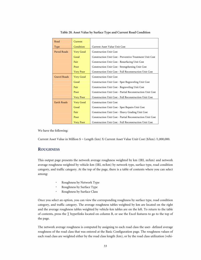
33

Table 20. Asset Value by Surface Type and Current Road Condition

Road Current

Type Condition Current Asset Value Unit Cost

Paved Roads Very Good Construction Unit Cost

Good Construction Unit Cost - Preventive Treatment Unit Cost

Fair Construction Unit Cost - Resurfacing Unit Cost

Poor Construction Unit Cost - Strengthening Unit Cost

Very Poor Construction Unit Cost - Full Reconstruction Unit Cost

Gravel Roads Very Good Construction Unit Cost

Good Construction Unit Cost - Spot Regraveling Unit Cost

Fair Construction Unit Cost - Regraveling Unit Cost

Poor Construction Unit Cost - Partial Reconstruction Unit Cost

Very Poor Construction Unit Cost - Full Reconstruction Unit Cost

Earth Roads Very Good Construction Unit Cost

Good Construction Unit Cost - Spot Repairs Unit Cost

Fair Construction Unit Cost - Heavy Grading Unit Cost

Poor Construction Unit Cost - Partial Reconstruction Unit Cost

Very Poor Construction Unit Cost - Full Reconstruction Unit Cost We have the following:

Current Asset Value in Million $ = Length (km) X Current Asset Value Unit Cost ($/km) /1,000,000.

ROUGHNESS

This output page presents the network average roughness weighted by km (IRI, m/km) and network

average roughness weighted by vehicle-km (IRI, m/km) by network type, surface type, road condition

category, and traffic category. At the top of the page, there is a table of contents where you can select

among:

Roughness by Network Type

Roughness by Surface Type

Roughness by Surface Class Once you select an option, you can view the corresponding roughness by surface type, road condition

category, and traffic category. The average roughness tables weighted by km are located on the right

and the average roughness tables weighted by vehicle-km tables are on the left. To return to the table

of contents, press the T hyperlinks located on column B, or use the Excel features to go to the top of

the page.

The network average roughness is computed by assigning to each road class the user- defined average

roughness of the road class that was entered at the Basic Configuration page. The roughness values of

each road class are weighted either by the road class length (km), or by the road class utilization (vehi-

34

cle-km) computed by multiplying the road class length by the average traffic of the road class defined

at the Basic Configuration page.

NETWORK DISTRIBUTION CHARTS

This output page presents network distribution charts of the network length, utilization, and maxi-

mum and current asset value by network type and surface type. The charts are produced from the re-

sults presented on the previous output pages.

NETWORK MONITORING INDICATORS

This page presents a road network monitoring indicators table and two user-defined charts. The road

network monitoring indicators table presents monitoring indicators by network type, subdivided into

the following categories.

Network Length

Network Density

Network Condition

Network Access

Network Standards

Network Utilization

Network Safety

Network Asset

You define the two charts to be presented below the network monitoring indicators table. Select the

two indicators to chart using the drop-down lists on cells B83 and B85, which have a yellow back-

ground.

Figure 4 shows the network monitoring indicators computed by RONET. The network access indica-

tor “All-weather roads area of influence (4 km wide) per land area” is a rough proxy of the interna-

tional Rural Access Indicator that measures the number of rural people who live within two kilometers

(typically equivalent to a walk of 20-25 minutes) of an all-season road as a proportion of the total rural

population 9.

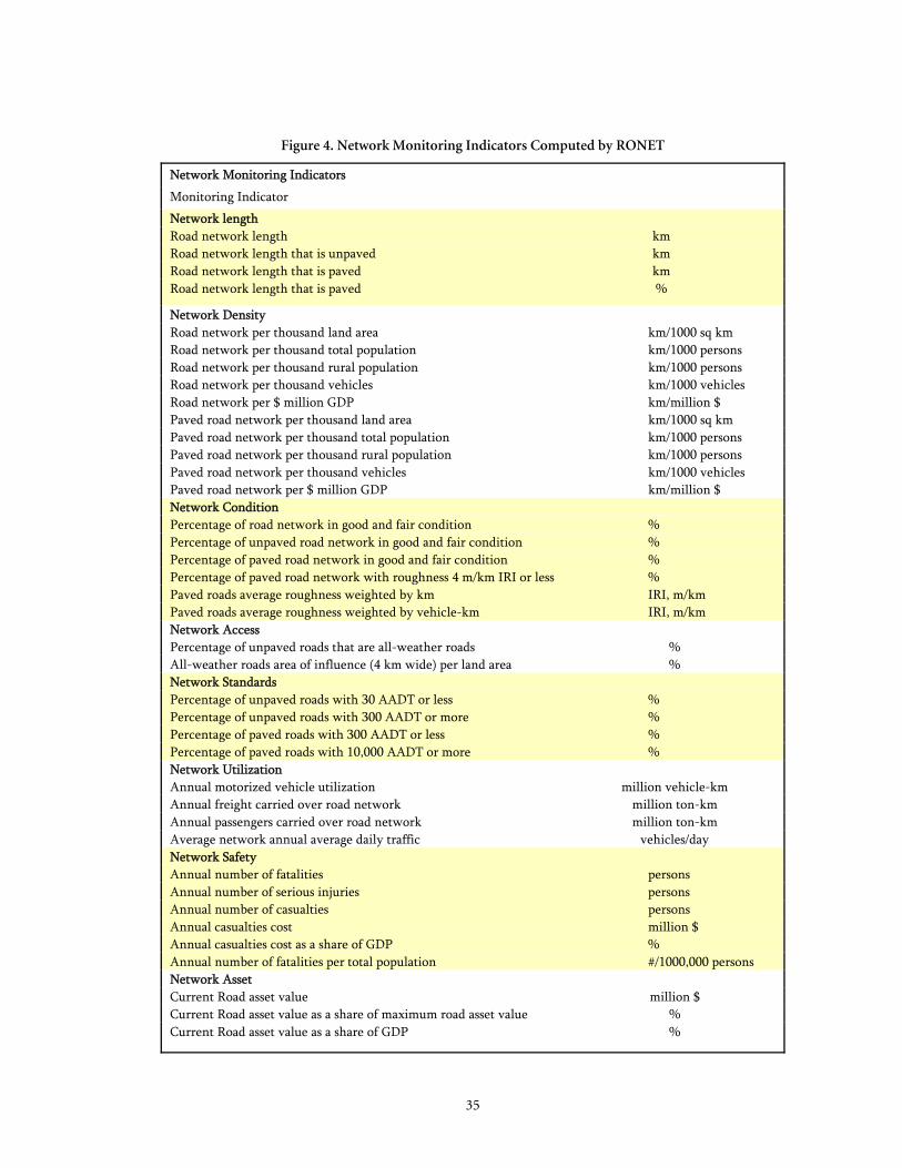
35

Figure 4. Network Monitoring Indicators Computed by RONET

Network Monitoring Indicators

Monitoring Indicator

Network length Road network length km Road network length that is unpaved km Road network length that is paved km Road network length that is paved %

Network Density Road network per thousand land area km/1000 sq km Road network per thousand total population km/1000 persons Road network per thousand rural population km/1000 persons Road network per thousand vehicles km/1000 vehicles Road network per $ million GDP km/million $ Paved road network per thousand land area km/1000 sq km Paved road network per thousand total population km/1000 persons Paved road network per thousand rural population km/1000 persons Paved road network per thousand vehicles km/1000 vehicles Paved road network per $ million GDP km/million $ Network Condition Percentage of road network in good and fair condition % Percentage of unpaved road network in good and fair condition % Percentage of paved road network in good and fair condition % Percentage of paved road network with roughness 4 m/km IRI or less % Paved roads average roughness weighted by km IRI, m/km Paved roads average roughness weighted by vehicle-km IRI, m/km Network Access Percentage of unpaved roads that are all-weather roads % All-weather roads area of influence (4 km wide) per land area % Network Standards Percentage of unpaved roads with 30 AADT or less % Percentage of unpaved roads with 300 AADT or more % Percentage of paved roads with 300 AADT or less % Percentage of paved roads with 10,000 AADT or more % Network Utilization Annual motorized vehicle utilization million vehicle-km Annual freight carried over road network million ton-km Annual passengers carried over road network million ton-km Average network annual average daily traffic vehicles/day Network Safety Annual number of fatalities persons Annual number of serious injuries persons Annual number of casualties persons Annual casualties cost million $ Annual casualties cost as a share of GDP % Annual number of fatalities per total population #/1000,000 persons Network Asset Current Road asset value million $ Current Road asset value as a share of maximum road asset value % Current Road asset value as a share of GDP %

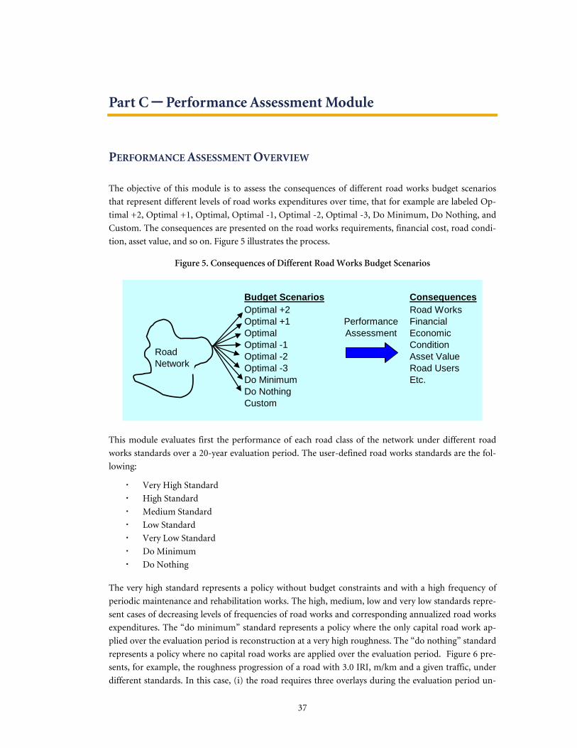
37

Part C – Performance Assessment Module

PERFORMANCE ASSESSMENT OVERVIEW

The objective of this module is to assess the consequences of different road works budget scenarios

that represent different levels of road works expenditures over time, that for example are labeled Op-

timal +2, Optimal +1, Optimal, Optimal -1, Optimal -2, Optimal -3, Do Minimum, Do Nothing, and

Custom. The consequences are presented on the road works requirements, financial cost, road condi-

tion, asset value, and so on. Figure 5 illustrates the process.

Figure 5. Consequences of Different Road Works Budget Scenarios

Budget Scenarios ConsequencesOptimal +2 Road WorksOptimal +1 Performance FinancialOptimal Assessment EconomicOptimal -1 ConditionOptimal -2 Asset ValueOptimal -3 Road UsersDo Minimum Etc.Do NothingCustom

RoadNetwork

This module evaluates first the performance of each road class of the network under different road

works standards over a 20-year evaluation period. The user-defined road works standards are the fol-

lowing:

Very High Standard

High Standard

Medium Standard

Low Standard

Very Low Standard

Do Minimum

Do Nothing

The very high standard represents a policy without budget constraints and with a high frequency of

periodic maintenance and rehabilitation works. The high, medium, low and very low standards repre-

sent cases of decreasing levels of frequencies of road works and corresponding annualized road works

expenditures. The “do minimum” standard represents a policy where the only capital road work ap-

plied over the evaluation period is reconstruction at a very high roughness. The “do nothing” standard

represents a policy where no capital road works are applied over the evaluation period. Figure 6 pre-

sents, for example, the roughness progression of a road with 3.0 IRI, m/km and a given traffic, under

different standards. In this case, (i) the road requires three overlays during the evaluation period un-

38

der the very high standard (years 1, 7 and 15); (ii) the road requires one overlay in year 7 under the

very low standard; and (iii) the “do-minimum” and “do-nothing” standards are equal and don’t exe-

cute any capital road work during the evaluation period because the road does not reached a rough-

ness level that merits reconstruction under the “do-minimum” standard.

Figure 6. Road Deterioration under Different Standards (level of service)

Once the performance of each road class is evaluated under the different standards, RONET presents

the corresponding results for a series of budget scenarios that are defined in one of the following three

possible evaluation options defined by the user:

Evaluation of Optimal Standard per Road Class

Evaluation of Custom Budged Scenario

Evaluation of Applying same Standard on all Road Classes

Evaluation of Optimal Standard per Road Class

In this evaluation option, for each road class, RONET evaluates the performance of the road class un-

der the different standards and calculates the corresponding stream of road agency costs (rehabilita-

tion and maintenance), road user costs and total society costs (sum of road agency and user costs)

over the evaluation period. RONET them computes the present value of the total society costs for each

standard, at the input discount rate, and determines the optimal standard for the road class, which is

the one that yields the lowest present value of total society costs.

The Optimal budget scenario represents a scenario of applying the optimal standard of each road class

on all the road classes that comprise the network. Once RONET determines the optimal scenario,

RONET defines the other budget scenarios as following:

0.0

1.0

2.0

3.0

4.0

5.0

6.0

7.0

0 2 4 6 8 10 12 14 16 18 20

Year

Roug

hnes

s (IR

I, m

/km

) Very High StandardHigh StandardMedium StandardLow StandardVery Low StandardDo MinimumDo Nothing

39

Optimal +1: for each road class RONET applies, if possible, a standard that is one level

higher than the optimal standard in terms of road agency expenditures. Some example: (i)

if the optimal standard is Medium Standard then RONET applies High Standard; (ii) if the

optimal standard is Low Standard then RONET applies Medium Standard; and (ii) if the

optimal standard is Very High Standard then RONET applies Very High Standard because

that is the upper limit.

Optimal +2: for each road class RONET applies, if possible, a standard that is two levels

higher than the optimal standard in terms of road agency expenditures. For example, if the

optimal standard is Medium Standard then RONET applies Very High Standard.

Optimal -1: for each road class RONET applies, if possible, a standard that is one level

lower than the optimal standard in terms of road agency expenditures. For example, if the

optimal standard is Medium Standard then RONET applies Low Standard.

Optimal -2: for each road class RONET applies, if possible, a standard that is two levels

lower than the optimal standard in terms of road agency expenditures. For example, if the

optimal standard is Medium Standard then RONET applies Very Low Standard.

Optimal -3: for each road class RONET applies, if possible, a standard that is three levels

lower than the optimal standard in terms of road agency expenditures. For example, if the

optimal standard is Medium Standard then RONET applies Do Minimum Standard. Note

that the lower limit is defined to be to apply the Do Minimum Standard and not the Do

Nothing Standard.

Do Minimum: RONET applies the Do Minimum Standard on all road classes

Do Nothing: RONET applies the Do Nothing Standard on all road classes

Custom: The user defines which standard to apply on each road class as a function of the

network type and traffic category of the road class.

The Optimal -1, Optimal -2, Optimal -3, Do Minimum and Do Nothing budget scenarios

represent network budget constrains, while Optimal +1 and Optimal +2 represent scenar-

ios of over spending in relation to the optimal scenario included on RONET to show the

consequences of over spending resources..

Evaluation of Custom Standard per Road Class

In this evaluation option, the user defines a Custom Budget Scenario by defining one standard to be

applied to each road class per network type and traffic level. RONET defines the other budget scenar-

ios as following:

Custom +1: for each road class RONET applies, if possible, a standard that is one level

higher than the custom standard in terms of road agency expenditures.

Custom +2: for each road class RONET applies, if possible, a standard that is two levels

higher than the custom standard in terms of road agency expenditures.

Custom -1: for each road class RONET applies, if possible, a standard that is one level

lower than the custom standard in terms of road agency expenditures.

40

Custom -2: for each road class RONET applies, if possible, a standard that is two levels

lower than the custom standard in terms of road agency expenditures.

Custom -3: for each road class RONET applies, if possible, a standard that is three levels

lower than the optimal standard in terms of road agency expenditures.

Do Minimum: RONET applies the Do Minimum Standard on all road classes

Do Nothing: RONET applies the Do Nothing Standard on all road classes

Evaluation of Applying Same Standard on all Road Classes

In this evaluation option, RONET defines the budget scenarios as:

Very High: RONET applies the very high standard on all road classes

High: RONET applies the high standard on all road classes

Medium: RONET applies the medium standard on all road classes

Low: RONET applies the low standard on all road classes

Very Low: RONET applies the very low standard on all road classes

Do Minimum: RONET applies the Do Minimum Standard on all road classes

Do Nothing: RONET applies the Do Nothing Standard on all road classes

Custom: The user defines which standard to apply on each road class as a function of the

network type and traffic category of the road class.

Performance Assessment Outputs

The outputs of this module are the following.

Network Performance: presents the consequences to the total, paved or unpaved network

of applying the different budget scenarios (road expenditure levels). Consequences are pre-

sented in terms of:

- Road Agency Costs

- Society Costs

- Road Users Costs

- Network Asset Value

- Network Roughness

- Network Condition

- Annual Road Agency Costs

- Annual Road Agency Costs by GDP

Annual Work Program: presents for the total, paved or unpaved network and for a user-

selected budget scenario, the stream of society costs, net benefits, road works, asset value,

and network condition.

41

Solution Catalog: presents for a user-selected budget scenario, the standards that will be

applied on each road class.

Road Works Distribution: presents, for a user-selected budget scenario, the distribution of

the recurrent maintenance, periodic maintenance and rehabilitation costs, and road works

length by network type, management type, surface type, and surface class, for years 1 to 5, 6

to 20 and 1 to 20. The output tables present: (i) total road works costs (M$); (ii) annual

road works costs (M$/year); (iii) annual road works costs per km ($/km-year); (iv) costs

per vehicle-km ($/vehicle-km) and (v) annual road works length (km/year).

Road Works Summary: presents for a user-selected budget scenario, period (years 1 to 5, 6

to 20 or 1 to 20), and road work type (recurrent maintenance, periodic maintenance, reha-

bilitation, or all works), a summary of the distribution, by network type, management type

and surface type, of the following: (i) road works costs; (ii) current network length, (iii)

current network utilization; and (iv) current network asset value. This output page also

presents a table with affordability indicators.

Historical Expenditures Comparison: presents, for a user-selected budget scenario, each

network type and road work type: (i) the historic expenditures over the last five years, (ii)

the required expenditures over the next five years, and (iii) the ratio between the required

per historic expenditures.

All the results are computed using Excel macros; therefore, you have to press the button “Performance

Assessment” located at the main menu to compute the results. The results are not recomputed auto-

matically when you change any configuration data or input data. When you press the button “Per-

formance Assessment,” RONET asks if you want to keep the intermediate results of the calculations in

a temporary workbook. If you select Yes, all the intermediate results are stored in a new workbook that

is created every time you select Yes at this option. The new workbooks are named “Book1,” “Book2,”

“Book3,” and so on. Once you have reviewed one of the temporary workbooks, you can close it or save

it if necessary (saving with a different name if necessary). If you select No, then no temporary work-

book is created. To compute the results can take between 2 and 5 minutes, depending on the com-

puter processing speed. The status of the calculations is presented on the Excel status line at the bot-

tom left corner of the screen. When all the calculations are done, the model presents a message indi-

cating the end of the calculations and the duration of the calculations.

The characteristics of the road works standards are country-specific; therefore, you define the charac-

teristics of the road works standards at the Standards Configuration page.

STANDARDS CONFIGURATION

The Standards Configuration page defines the characteristics of the road work standards to be evalu-

ated at the Performance Assessment Module, which estimates the road deterioration of each road class

under seven possible standards (Very High, High, Medium, Low, Very Low, Do Minimum and Do

Nothing). The inputs on this page do not affect the results of the current condition assessment mod-

ule. On this page, you configure the following.

42

Custom Budget Scenario

Budget Scenarios Evaluation Option

Capital Road Works Standards

Recurrent Maintenance Works Standards

Custom Budget Scenario

The custom budget scenario definition table is used to define the custom scenario to be evaluated. On

this table, you define for each network type and traffic category the road work standard that will be

applied under this custom scenario. For example, one can define to apply the very high standard on

Motorways and Primary roads with high traffic and the low standard on Tertiary and Unclassified

roads with low traffic. The custom scenario summarizes the overall results of applying the selected

standards on the corresponding network types and traffic categories. The default values are given in

table 21. These are country- or study-specific values; therefore, it is expected that you will change these

values.

Table 21. Custom Budget Scenario Definition

Custom Budget Scenario StandardsTraffic Category

Code Network Type Traffic I Traffic II Traffic III Traffic IV Traffic VH Motorways Very Low Standard Low Standard Medium Standard High Standard Very High StandardI Primary Very Low Standard Low Standard Medium Standard High Standard Very High StandardJ Secondary Very Low Standard Low Standard Medium Standard High Standard Very High StandardK Tertiary Very Low Standard Low Standard Medium Standard High Standard Very High StandardL Unclassified Very Low Standard Low Standard Medium Standard High Standard Very High Standard

Budget Scenarios Evaluation Option

Here you define your choice for the definition of the budget scenarios to be the evaluated by RONET.

You select an evaluation option by selecting one of the available option buttons as shown on Table 22.

Table 22. Budget Scenarios Evaluation Option

Budget Scenarios Evaluation Option

Evaluation of optimal standard per road class (lowest total society costs and highest NPV)

Evaluation of custom standard per road class (user-defined standard)

Evaluation of applying same standard on all road classes

Capital Road Works Standards Configuration

This table defines the capital road works (periodic maintenance and rehabilitation works) to be ap-

plied on each standard to be evaluated. The default values for concrete and asphalt concrete roads are

given below in table 23. Most likely these default values are applicable for most countries worldwide;

therefore, it is expected that few users will modify these default values.

Table 23. Cement Concrete and Asphalt Mix Roads Default Values

Roughness Thresholds to Apply Recommended Road Works (IRI, m/km)

43

Roughness Range and Required Road Work

Scenario IRI<=4.0 Overlay

4.0<IRI<=6.0 Overlay

6.0<IRI<=8.0 Strengthening

8.0<IRI<=10.0 Reconstruction

10<IRI Reconstruction

Code Name Roughness Threshold (IRI)

A Very High Standard 3.00 4.00 6.00 8.00 10.00

B High Standard 3.25 4.50 6.50 8.50 10.50

C Medium Standard 3.50 5.00 7.00 9.00 11.00

D Low Standard 3.75 5.50 7.50 9.50 11.50

E Very Low Standard 4.00 6.00 8.00 10.00 12.00

F Do Minimum 99.00 99.00 99.00 99.00 14.00

G Do Nothing 99.00 99.00 99.00 99.00 99.00 On this table you define, for each roughness range, the roughness thresholds when the required capital

road works will be applied. For example, for a road with current roughness of less than 4.0 IRI, on a

very high standard scenario, the required overlay (periodic maintenance) will be applied when the

road reaches 3.0 IRI; and on a very low standard scenario, when the road reaches 4.0 IRI. For roads

with less than 6.0 IRI, the required road works are overlays; for roads between 6.0 and 8.0 IRI, the re-

quired road works are thick overlays (strengthening), and for roads with roughness higher than 8.0

IRI, the required road works are reconstructions. The default values for surface treatment roads are

given in table 24. Most likely these default values are applicable for most countries worldwide; there-

fore, it is expected that few users will modify these default values.

Table 24. Default Values for Surface Treatment Roads

Time Interval and Roughness Thresholds to Apply Recommended Road Works (IRI, m/km)

Roughness Range and Required Road Work

Scenario

IRI<=4.0 Reseal

4.0<IRI<=7.0 Reseal

7.0<IRI<=9.0 Strengthening

9.0<IRI<=11.0 Reconstruction

11<IRI Reconstruction

Code Name Time Interval (years) Roughness Threshold (IRI) A Very High Standard 7 7 7.00 9.00 11.00

B High Standard 9 9 7.50 9.50 11.50

C Medium Standard 11 11 8.00 10.00 12.00

D Low Standard 13 13 8.50 10.50 12.50

E Very Low Standard 15 15 9.00 11.00 13.00

F Do Minimum 99 99 99.00 99.00 15.00

G Do Nothing 99 99 99.00 99.00 99.00

In this case, reseals are the work required for roads with roughness less than 7.0 IRI, and the reseals are

scheduled at a fixed time interval in years. On this table, you define, for each roughness range, the

roughness thresholds when the required capital road works will be applied for roads with roughness

higher than 7.0 IRI, and the frequency of the reseals for roads with roughness less than 7.0 IRI. For

example, for a road with current roughness less than 4.0 IRI, on a very high standard scenario, the

required reseal (periodic maintenance) will be applied every seven years, and on a very low standard

scenario, every 15 years.

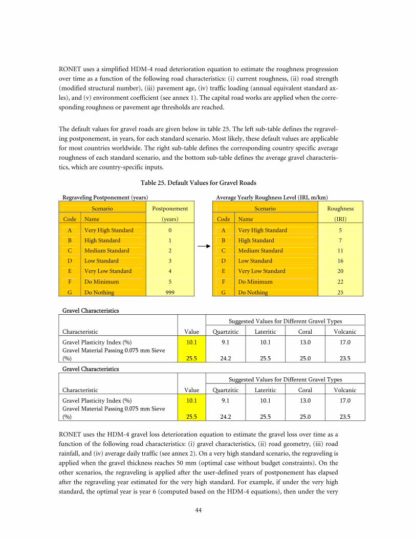
44

RONET uses a simplified HDM-4 road deterioration equation to estimate the roughness progression

over time as a function of the following road characteristics: (i) current roughness, (ii) road strength

(modified structural number), (iii) pavement age, (iv) traffic loading (annual equivalent standard ax-

les), and (v) environment coefficient (see annex 1). The capital road works are applied when the corre-

sponding roughness or pavement age thresholds are reached.

The default values for gravel roads are given below in table 25. The left sub-table defines the regravel-

ing postponement, in years, for each standard scenario. Most likely, these default values are applicable

for most countries worldwide. The right sub-table defines the corresponding country specific average

roughness of each standard scenario, and the bottom sub-table defines the average gravel characteris-

tics, which are country-specific inputs.

Table 25. Default Values for Gravel Roads

Regraveling Postponement (years) Average Yearly Roughness Level (IRI, m/km)

Scenario Postponement Scenario Roughness

Code Name (years) Code Name (IRI)

A Very High Standard 0 A Very High Standard 5

B High Standard 1 B High Standard 7

C Medium Standard 2

C Medium Standard 11

D Low Standard 3 D Low Standard 16

E Very Low Standard 4 E Very Low Standard 20

F Do Minimum 5 F Do Minimum 22

G Do Nothing 999 G Do Nothing 25

Gravel Characteristics

Suggested Values for Different Gravel Types

Characteristic Value Quartzitic Lateritic Coral Volcanic

Gravel Plasticity Index (%) 10.1 9.1 10.1 13.0 17.0 Gravel Material Passing 0.075 mm Sieve (%) 25.5 24.2 25.5 25.0 23.5

Gravel Characteristics

Suggested Values for Different Gravel Types

Characteristic Value Quartzitic Lateritic Coral Volcanic

Gravel Plasticity Index (%) 10.1 9.1 10.1 13.0 17.0 Gravel Material Passing 0.075 mm Sieve (%) 25.5 24.2 25.5 25.0 23.5

RONET uses the HDM-4 gravel loss deterioration equation to estimate the gravel loss over time as a

function of the following road characteristics: (i) gravel characteristics, (ii) road geometry, (iii) road

rainfall, and (iv) average daily traffic (see annex 2). On a very high standard scenario, the regraveling is

applied when the gravel thickness reaches 50 mm (optimal case without budget constraints). On the

other scenarios, the regraveling is applied after the user-defined years of postponement has elapsed

after the regraveling year estimated for the very high standard. For example, if under the very high

standard, the optimal year is year 6 (computed based on the HDM-4 equations), then under the very

45

low standard, the regraveling is applied on year 10 after the user-defined four years of postponement.

The regraveling frequency and the recurrent maintenance determine the average roughness of gravel

roads. On RONET, the average roughness of gravel roads for each standard is not computed using

some equations; it is user-defined in the right sub-table.

The default values for earth roads are given below in table 26. The left sub-table defines the heavy

grading interval, in years, for each standard scenario. Most likely, these default values are applicable

for most countries worldwide. The right sub-table defines the corresponding average roughness of

each standard scenario. These are country-specific inputs.

Table 26. Default Values for Earth Roads

Earth Roads Heavy Grading Interval (years) Average Yearly Roughness Level (IRI, m/km)

Scenario Interval Scenario Roughness

Code Name Years Code Name (IRI)

A Very High Standard 2 A Very High Standard 7

B High Standard 4 B High Standard 9

C Medium Standard 6 C Medium Standard 13

D Low Standard 8 D Low Standard 18

E Very Low Standard 10 E Very Low Standard 22

F Do Minimum 12 F Do Minimum 24

G Do Nothing 999 G Do Nothing 25

RONET adopts the user-defined time interval of heavy grading to characterize each standard scenario.

The interval of heavy grading and the recurrent maintenance determine the average roughness of earth

roads. On RONET, the average roughness of earth roads for each standard is not computed using

some equations; it is user-defined in the right sub-table.

Recurrent Maintenance Works Standards Configuration

Table 27 defines the recurrent maintenance works costs multipliers to be applied on each of the stan-

dards to be evaluated. The default values are given in table 26. Most likely these default values are ap-

plicable for most countries worldwide; therefore, it is expected that few users will modify these default

values.

Table 27. Recurrent Maintenance Works Standards Configuration

Scenario Surface Type

Code Name Concrete Asphalt S.T. Gravel Earth

A Very High Standard 1.00 1.00 1.00 1.00 1.00

B High Standard 1.00 1.00 1.00 1.00 1.00

C Medium Standard 1.00 1.00 1.00 1.00 1.00

D Low Standard 0.50 0.50 0.50 0.50 0.50

E Very Low Standard 0.50 0.50 0.50 0.50 0.50

F Do Minimum 0.25 0.25 0.25 0.25 0.25

G Do Nothing 0.00 0.00 0.00 0.00 0.00

46

On this table you define, for each surface type, the recurrent maintenance cost multipliers applicable

to each standard scenario. For example, for the very high standard scenario, for asphalt roads, the re-

current maintenance costs defined at the Country Data page are multiplied by 1.00, whereas for the

very low standard scenario, the recurrent maintenance costs defined at the Country Data page are

multiplied by 0.50. Note that the average roughness of unpaved roads (defined before) is greatly re-

lated to the level of expenditures for recurrent maintenance of unpaved roads; therefore, you have to

enter coherent values in both tables.

Paved Roads Deterioration Calibration Coefficients

This table allows for configuring the paved roads deterioration calibration coefficients for concrete,

asphalt, and surface treatment roads. The a1 coefficient multiplies the modified structural number of

the road, and the a2 coefficient multiplies the pavement age to replace the surface distress and rutting

components of the roughness deterioration (see annex 1). It is expected that few users will modify

these default values, and will do so only after performing an HDM-4 roughness progression calibra-

tion effort.

HISTORICAL EXPENDITURES

On this page you enter (i) the historical average road works expenditures during the last five years, in

M$ per year, and (ii) the historical average road works during last five years, in km per year. You can

enter this information by network type, road work type (rehabilitation, periodic maintenance, routine

maintenance, and total), and surface class (paved, unpaved, and total). RONET computes on this page

the corresponding average road works expenditures during the last five years, in $ per km, for the dif-

ferent road work types and surface classes.

The information entered into this page is used by the Performance Assessment Module to compare the

required expenditure under different road work scenarios with the historical expenditures in the

country.

NETWORK PERFORMANCE

This page presents the consequences of different budget scenarios (road expenditure levels). The con-

sequences are presented in terms of:

Road Agency Costs

Society Costs

Road Users Costs

Network Asset Value

Network Roughness

Network Condition

Annual Road Agency Costs

Annual Road Agency Costs by GDP

47

On cell D1, you select, from the list of available choices, whether you want to view the consequences to

the paved, unpaved, or total network. At the top of the page, there is a table of contents where you can

select among:

Total Society Costs and Net Benefits Charts

Consequences to Road Agency

Consequences to Society

Consequences to Road Users

Consequences to Network Asset Value and Network Roughness

Consequences to Network Condition 1/2

Consequences to Network Condition 2/2

Consequences to Annual Road Agency Costs

Consequences to Annual Road Agency Costs by GDP Once you select an option, you can view the corresponding tables and charts. To return to the table of

contents, press the T hyperlinks located on column B or use the Excel features to go to the top of the

page.

The available tables and charts are the following:

Total Society Costs and Net Benefits Charts

- Chart of present value, at the defined discount rate, of road agency, road user, and

total society costs

- Chart o present value of net benefits compared with the present value of road agency

costs

Consequences to Road Agency

- Road Agency Costs (Years 1-20)

- Road Agency Costs Breakdown (Years 1-20)

- Recurrent Maintenance as a Percent of Total Maintenance Costs

Consequences to Society

- Society Costs (Total Costs Years 1-20)

- Society Net Loss Compared to Very High Standard (Total Costs Years 1-20)

- Society Net Benefits Compared to Do Minimum Standard (Total Costs Years 1-20)

Consequences to Road Users

- Impact of Road Agency Deficit on Road User Costs

- Unit Road User Costs

Consequences to Network Asset Value and Network Roughness

- Network Asset Value

- Roughness Weighted by Km

- Roughness Weighted by Vehicle-Km

Consequences to Network Condition 1/2

- Network Length in Very Good Condition

- Network Length in Good Condition

- Network Length in Fair Condition

48

Consequences to Network Condition 2/2

- Network Length in Poor Condition

- Network Length in Very Poor Condition

- Network Length by Road Condition (select the budget scenario for this table on cell

D402)

Consequences to Annual Road Agency Costs

- Annual Road Agency Costs Years 1-5 (Annual Costs Years 1-5)

- Annual Road Agency Costs Years 6-20 (Annual Costs Years 6-20)

- Annual Road Agency Costs Years 1-20 (Annual Costs Years 1-20)

Consequences to Annual Road Agency Costs by GDP

- Annual Road Agency Costs Years 1-5 (Percentage of GDP)

- Annual Road Agency Costs Years 6-20 (Percentage of GDP)

- Annual Road Agency Costs Years 1-20 (Percentage of GDP)

Consequences to Present Value Costs 1/2

- Present Value of Road Agency Costs

- Present Value of Society Costs

- Present Value Society Net Loss Compared to Optimal Scenario

Consequences to Present Value Costs 2/2

- Present Value Society Net Benefits Compared to Do Minimum Standard (NPV)

- Present Value Impact of Road Agency Deficit on Road User Costs

ANNUAL WORK PROGRAM

This page presents the annual work program for a user-selected budget scenario and road network. On

cell C1, you select, from the list of available choices, a budget scenario. On cell E1, you select, from the

list of available choices, whether you want to view the work program for the paved, unpaved, or total

network. The output table presents the following annual values:

Costs (million $)

- Rehabilitation

- Periodic Maintenance

- Recurrent Maintenance

- Road Agency

- Road Users

- Total Society

Net Benefit Compared with Do Minimum Scenario (million $)

Asset Value (million $)

Annual Road Works (km)

- Rehabilitation

- Periodic Maintenance

- Recurrent Maintenance

Road Condition

- Roughness Weighted per Km

49

- Roughness Weighted per Vehicle-Km

The output table also presents the totals in years 1-5, 6-20 and 1-20, annual values in these periods,

and present values over the evaluation period, as well as the average network roughness over the

evaluation period.

SOLUTION CATALOG

This page presents, for a user-selected budget scenario, the standards that RONET selected for each

road class for the given budget scenario. On cell C1, you select, from the list of available choices, a

budget scenario. Each standard is assigned a number that is presented on the solution catalog table.

ROAD WORKS DISTRIBUTION

This page presents, for a user-selected budget scenario, for the recurrent maintenance works, periodic

maintenance works, rehabilitation works, and all works, the following information:

Total road works costs (M$)

Annual road works costs (M$/year)

Annual road works costs per km ($/km-year)

Road works per vehicle-km ($/vehicle-km)

Annual road works length (km/year)

The information is presented by network type, management type, surface class and surface type, and

for years 1 to 5, 6 to 20 and 1 to 20. On cell C1, you select, from the list of available choices, a budget

scenario. At the top of the page, there is a table of contents where you can select among:

Total Road Works Costs (M$) by Network Type and Surface Class

Annual Road Works Costs (M$/year) by Network Type and Surface Class

Annual Road Works Costs per Km ($/km-year) by Network Type and Surface Class

Road Works per Vehicle-km ($/vehicle-km) by Network Type and Surface Class

Annual Road Works Length (km/year) by Network Type and Surface Class

Total Road Works Costs (M$) by Management Type and Surface Class

Annual Road Works Costs (M$/year) by Management Type and Surface Class

Annual Road Works Costs per Km ($/km-year) by Management Type and Surface Class

Road Works per Vehicle-km ($/vehicle-km) by Management Type and Surface Class

Annual Road Works Length (km/year) by Management Type and Surface Class

Total Road Works Costs (M$) by Network Type and Surface Type

Annual Road Works Costs (M$/year) by Network Type and Surface Type

Annual Road Works Costs per Km ($/km-year) by Network Type and Surface Type

50

Road Works per Vehicle-km ($/vehicle-km) by Network Type and Surface Type

Annual Road Works Length (km/year) by Network Type and Surface Type

Total Road Works Costs (M$) by Management Type and Surface Type

Annual Road Works Costs (M$/year) by Management Type and Surface Type

Annual Road Works Costs per Km ($/km-year) by Management Type and Surface Type

Road Works per Vehicle-km ($/vehicle-km) by Management Type and Surface Type

Annual Road Works Length (km/year) by Management Type and Surface Type

Once you select an option, you can view the corresponding tables. To return to the table of contents,

press the T hyperlinks located on columns B or T, or use the Excel features to go to the top of the page.

ROAD WORKS SUMMARY

This page presents affordability indicators and a summary of the distribution of the network:

Road works costs

Current network length

Current network utilization

Current network asset value

The distribution is presented by network type, management type, and surface type.

On cell C1, you select, from the list of available choices, a budget scenario. On cell F1, you select a road

works type (recurrent maintenance works, periodic maintenance works, rehabilitation works, capital

works, or all works) and on cell I1 you select a period (year 1 to 5, 6 to 20 or 1 to 20). At the top of the

page, there is a table of contents where you can select among:

Affordability Indicators

Information by Network Type

Information by Surface Type

Information by Management Type

Once you select an option, you can view the corresponding tables. To return to the table of contents,

press the T hyperlinks located on column B, or use the Excel features to go to the top of the page.

HISTORICAL EXPENDITURES COMPARISON

This page presents, for a user-selected budget scenario, each network type and road work type: (i) the

historic expenditures over the last five years, (ii) the required expenditures over the next five years,

and (iii) the ratio between the required per historic expenditures. Similar tables are presented for the

annual road works length, comparing the historical works, the required works and the ratio the re-

quired and historic works. On cell C1, you select, from the list of available choices, a budget scenario.

51

Part D – Road User Revenues Module

ROAD USER REVENUES OVERVIEW

The objective of this module is to estimate road user revenues collected from road user charges and to

compare these revenues with the network funding requirements. Revenues computed are originated

from fuel levies, new vehicle registration fees, license and inspection fees, insurance and other fees,

load damage fees, distance travel fees, international transit revenues, tolls revenues, foreign vehicle

permit revenues, vignettes revenues, carbon tax revenues, traffic enforcement revenues and other fees

and taxes revenues. The funding requirements are defined for routine maintenance, periodic mainte-

nance, rehabilitation, investments, administration and other expenditures. In other words, RONET

determines the level of road user charges required to meet the funding requirements for a given

budget scenario and the actual funding gap.

VEHICLE FLEET CONFIGURATION

The Vehicle Fleet Configuration page defines the composition, utilization and fuel consumption char-

acteristics of the vehicle fleet. The inputs on this page do not affect the results of the Current Condi-

tion Assessment or the Performance Assessment modules. The default values are given in table 28,

which are country or study specific; therefore, it is expected that users will modify these default values.

Table 28. Vehicle Fleet Configuration Vehicle Fleet Configuration

Vehicle Fleet Annual Utilization Fuel ConsumptionCountry Country Kilometers Vehicle Fuel Annual Fuel Consumption

Fuel Type Fleet Vehicle Driven Utilization Consumption Diesel Gasoline Total(Diesel or Composition Fleet per Year (million (liters/ (million (million (million

Vehicle Type Gasoline) (%) (veh) (km/yr) veh-km/yr) veh-km) liters/yr) liters/yr) liters/yr)Motorcycle G 0% 0 15,000 0 0.05 0 0 0Car (Gasoline) G 45% 45,000 25,000 1,125 0.12 0 135 135Car (Diesel) D 5% 5,000 25,000 125 0.12 15 0 15Utility (Gasoline) G 20% 20,000 35,000 700 0.12 0 84 84Utility (Diesel) D 5% 5,000 35,000 175 0.12 21 0 21Truck Light D 10% 10,000 35,000 350 0.15 53 0 53Truck Medium D 8% 8,000 50,000 400 0.23 92 0 92Truck Heavy D 2% 2,000 70,000 140 0.43 60 0 60Truck Articulated D 1% 1,000 80,000 80 0.64 51 0 51Bus Light D 1% 1,000 50,000 50 0.14 7 0 7Bus Medium D 2% 2,000 70,000 140 0.21 29 0 29Bus Heavy D 1% 1,000 80,000 80 0.29 23 0 23Total 100% 100,000 3,365 0.17 352 219 571

Annual fuel consumption (million gallons/yr) 93 58 151Annual fuel consumption (000 ton/yr) 299 164 463

New vehicles registered per year 10,000Percent of trucks overloaded 10% At the Country Data input page, you define the total number of vehicles in use in the country. At the

Vehicle Fleet Configuration page, you define up to twelve vehicle types, the fuel type of each vehicle

type (enter D for Diesel or G for Gasoline), the composition of the vehicle fleet, the kilometers driven

per year, and the average unit fuel consumption, in liters/km. RONET computes the corresponding

52

total vehicle fleet utilization (million vehicle-km/year) and total annual diesel and gasoline fuel con-

sumption, in million liters/year, million gallons/year and thousand tons per year. At this page, you also

define the number of new vehicles registered each year and the percent of trucks that travel overloaded

and should be subject to load damage fines.

The Vehicle Fleet Configuration page allows you to check if the network utilization computed at the

Current Condition Assessment module, based on the distribution of the road network length by road

classes, is consistent with the network utilization computed from the vehicle fleet data entered at the

Vehicle Fleet Configuration page. A source of discrepancy could be the fact that the network being

evaluated at the Current Condition Assessment module does not include urban streets and avenues,

while the country vehicle fleet includes vehicles located in urban centers. Therefore, on this page you

can enter your estimate for the urban centers vehicle utilization and compare the calculation of the

total vehicle utilization from both methods. At this page, you can also check (i) if the total country

fuel consumption entered in the Country data is consistent with the fuel consumption computed at

this page; and (ii) if the fatalities computed at the current condition assessment monitoring indicators

is consistent with the total country fatalities entered in the Country data. Table 29 show the tables used

for checking these consistencies. You should modify your inputs either at the Road Network Length

page and/or the Vehicle Fleet Configuration page until you obtain a satisfactory consistency.

Table 29. Check Utilization and Fuel Consumption Consistency

Check Vehicle Utilization Consistency Check Fuel Consumption Consistency

Utilization from Matrix of Road Classes Consumption from Country DataMotorways 0 Diesel consumption (million liters) 350Primary 1,694 Gasoline consumption (million liters) 210Secondary 383Tertiary 72 Consumption from Vehicle Fleet DataUnclassified 0 Diesel consumption (million liters) 352Total (million veh-km/yr) 2,149 Gasoline consumption (million liters) 219Urban Streets & Avenues (million veh-km/yr) 1,000Grand Total (million veh-km/yr) 3,149

Utilization from Vehicle Fleet DataTotal (million veh-km/yr) 3,365

Check Fatalities Consistency

Fatalities from Matrix of Road ClassesMotorwaysPrimary 169Secondary 38Tertiary 7UnclassifiedTotal (persons/yr) 215

Fatalities from Country DataTotal country fatalities (persons/yr) 470

ROAD USER CHARGES

At this page you enter the road user charges that represent actual payments of road users. You have to

enter the current road user charges broken down by type and assignment. Road user charges are com-

posed of the following types:

53

Diesel and gasoline levies (cents $/liter)

Annual new vehicle registration fees ($/vehicle-year)

Annual vehicle license and inspection fees ($/vehicle-year)

Annual insurance and other fees ($/vehicle-year)

Annual road damage fee ($/vehicle-year)

Annual distance travel fee (cents $/km)

International transit revenues ($/transit)

Tolls revenues (cents $/km)

Foreign vehicle permit revenues ($/vehicle-year)

Vignettes revenues ($/vehicle-year)

Carbon taxes revenues ($/vehicle-year)

Traffic enforcement revenue ($/vehicle-year)

Other fees and taxes revenues ($/vehicle-year)

Under this model framework, road user charges and taxes can be assigned to the road sector or as-

signed to the general budget. It is usually the Ministry of Finance or the treasury which is the initial

recipient of the road user charges and they are then allocated to road funds, ministry of public works,

urban road agencies, etc. depending on the local institutional set up and the legislation. You have the

following options for road user charges assignment, as shown on Table 30:

Assigned to the Road Sector

- Road Fund

- Urban Road Entities

- Other Road Entities

Assigned to general budget

Table 30. Road User Charges Assignment Sample

Road User Charges

Fuel ConsumptionFuel Levy Assigned to the Road Sector Taxes Assigned Total

Road Urban Other Total to General RoadFuel Fund Road Entities Road Entities Road Sector Budget User Charges

Revenue Source Type (cent$/liter) (cent$/liter) (cent$/liter) (cent$/liter) (cent$/liter) (cent$/liter)Fuel Consumption Diesel 5.00 5.00 5.00 10.00

Gasoline 5.00 5.00 15.00 20.00

Vehicle FeesAssigned to the Road Sector Assigned Total

Number of Road Urban Other Total General RoadVehicle Vehicles per Year Fund Road Entities Road Entities Road Sector Budget User Charges

Revenue Source Type (vehicles/year) ($/vehicle) ($/vehicle) ($/vehicle) ($/vehicle) ($/vehicle) ($/vehicle)Vehicle Motorcycle 0 5.60 5.60 5.60New Vehicle Car (Gasoline) 4,500 22.00 22.00 22.00Registration Car (Diesel) 500 22.00 22.00 22.00Fees Utility (Gasoline) 2,000 33.00 33.00 33.00

Utility (Diesel) 500 33.00 33.00 33.00Truck Light 1,000 33.00 33.00 33.00Truck Medium 800 72.00 72.00 72.00Truck Heavy 200 130.00 130.00 130.00

54

To compute the international transit revenues and the tolls revenues, you will also need to enter at this

page the estimated annual number of transits and annual number of vehicle-kilometers travelled on

toll roads per vehicle type.

Because a percentage of the road user charges revenues are used to cover the collection process costs,

at this page, you also enter, for each road user charges source, the percent of revenues that represent

the collection costs or fees, for example, for administration purposes, as shown on table 31. RONET

computes and presents at the output pages, the effective road user charges revenues considering the

reduction in the gross revenues due to the collection process.

Table 31. Road User Charges Lost During Collection Process

Percent of Gross Revenues Consumed During Collection Process

Percent ofRevenue Source Revenues (%)Fuel Consumption 10%New Vehicle & Registration Fees 10%License & Inspection Fees 10%Insurance & Other Vehicle Fees 10%Road Damage Fees 10%Distance Travel Fees 10%International Transit Revenues 10%Tolls Revenues 10%Foreign Vehicle Permit Revenues 10%Vignettes Revenues 10%Carbon Taxes Revenues 10%Traffic Enforcement Revenues 10%Other Fees & and Taxes Revenues 10%

FUNDING REQUIREMENTS

At this page you define, per network type, the network annualized funding requirements in yeas 1 to 5,

6 to 10, or 1 to 20, which are composed of the following expenditures: (i) routine maintenance, (ii)

periodic maintenance, (iii) rehabilitation, (iv) investments, and (v) administration and other. The

routine maintenance, periodic maintenance and rehabilitation expenditures are the ones computed at

the Performance Assessment module for a user-selected budget scenario. On cell B1, you select, from

the list of available choices, the budget scenario, and on cell D1, you select, from the list of available

choices, the budget period. The routine maintenance, periodic maintenance and rehabilitation expen-

ditures are broken down for roads currently in stable condition (very good, good and fair condition)

and road not in stable condition (poor and very poor roads). You have to enter your estimates of an-

nualized investments, administration and other expenditures per network type, in million $/year, as

shown on Table 32. There are two additional user-defined options for investment expenditures and

three for administration and other expenditures.

55

Table 32. Annualized Funding Requirements

Optimal Scenario

Annualized Funding Requirements Years 1-5

Motorways Primary Secondary Tertiary Unclassified TotalRoutine Maintenance Very Good, Good and Fair Roads 0.00 1.56 1.89 0.17 0.00 3.61

Poor and Very Poor Roads 0.00 0.64 1.95 1.50 0.00 4.08Subtotal (M$/year) 0.00 2.19 3.84 1.67 0.00 7.70

Periodic Maintenance Very Good, Good and Fair Roads 0.00 12.03 2.07 0.10 0.00 14.20Poor and Very Poor Roads 0.00 0.21 2.32 2.85 0.00 5.37Subtotal (M$/year) 0.00 12.23 4.39 2.94 0.00 19.57

Rehabilitation Very Good, Good and Fair Roads 0.00 0.06 2.40 0.92 0.00 3.38Poor and Very Poor Roads 0.00 15.27 23.51 21.58 0.00 60.37Subtotal (M$/year) 0.00 15.33 25.91 22.51 0.00 63.75

Investment Expenditures New Construction (M$/year) 0.00Upgrading (M$/year) 0.00Widening (M$/year) 0.00

0.000.00

Other (M$/year) 0.00Subtotal (M$/year) 0.00 0.00 0.00 0.00 0.00 0.00

Administration and Other Administration (M$/year) 1.00 1.00 1.00 3.00Expenditures Road Safety (M$/year) 0.00

0.000.000.00

Other (M$/year) 0.00Subtotal (M$/year) 0.00 1.00 1.00 1.00 0.00 3.00

Total Expenditures Total (M$/year) 0.00 30.76 35.14 28.12 0.00 94.01 Because not all funding requirements should necessarily be financed by road user charges, at this page,

you also enter the percent of the funding requirements to be financed by road user charges as shown

in Table 33. RONET computes at the bottom of the page, the resulting annualized funding require-

ments to be financed by road user charges (see Table 34).

Table 33. Annualized Funding Requirements

Percent of Funding Requirements to be Financed by Road User Charges

Motorways Primary Secondary Tertiary UnclassifiedRoutine Maintenance Very Good, Good and Fair Roads 100% 100% 100% 100% 100%

Poor and Very Poor Roads 100% 100% 100% 100% 100%Periodic Maintenance Very Good, Good and Fair Roads 100% 100% 100% 100% 100%

Poor and Very Poor Roads 100% 100% 100% 100% 100%Rehabilitation Very Good, Good and Fair Roads 100% 100% 100% 100% 100%

Poor and Very Poor Roads 100% 100% 100% 100% 100%Investment Expenditures New Construction (M$/year) 100% 100% 100% 100% 100%

Upgrading (M$/year) 100% 100% 100% 100% 100%Widening (M$/year) 100% 100% 100% 100% 100%

100% 100% 100% 100% 100%100% 100% 100% 100% 100%

Other (%) 100% 100% 100% 100% 100%Administration and Other Administration (%) 100% 100% 100% 100% 100%Expenditures Road Safety (%) 100% 100% 100% 100% 100%

100% 100% 100% 100% 100%100% 100% 100% 100% 100%100% 100% 100% 100% 100%

Other (%) 100% 100% 100% 100% 100%

56

Table 34. Annualized Funding Requirements to be Cover by Road User Charges

Annualized Funding Requirements Years 1-5 to be Financed by Road User Charges

Motorways Primary Secondary Tertiary Unclassified TotalRoutine Maintenance Very Good, Good and Fair Roads 0.00 1.56 1.89 0.17 0.00 3.61

Poor and Very Poor Roads 0.00 0.64 1.95 1.50 0.00 4.08Subtotal (M$/year) 0.00 2.19 3.84 1.67 0.00 7.70

Periodic Maintenance Very Good, Good and Fair Roads 0.00 12.03 2.07 0.10 0.00 14.20Poor and Very Poor Roads 0.00 0.21 2.32 2.85 0.00 5.37Subtotal (M$/year) 0.00 12.23 4.39 2.94 0.00 19.57

Rehabilitation Very Good, Good and Fair Roads 0.00 0.06 2.40 0.92 0.00 3.38Poor and Very Poor Roads 0.00 15.27 23.51 21.58 0.00 60.37Subtotal (M$/year) 0.00 15.33 25.91 22.51 0.00 63.75

Investment Expenditures New Construction (M$/year) 0.00 0.00 0.00 0.00 0.00 0.00Upgrading (M$/year) 0.00 0.00 0.00 0.00 0.00 0.00Widening (M$/year) 0.00 0.00 0.00 0.00 0.00 0.00

0.00 0.00 0.00 0.00 0.00 0.000.00 0.00 0.00 0.00 0.00 0.00

Other (M$/year) 0.00 0.00 0.00 0.00 0.00 0.00Subtotal (M$/year) 0.00 0.00 0.00 0.00 0.00 0.00

Administration and Other Administration (M$/year) 0.00 1.00 1.00 1.00 0.00 3.00Expenditures Road Safety (M$/year) 0.00 0.00 0.00 0.00 0.00 0.00

0.00 0.00 0.00 0.00 0.00 0.000.00 0.00 0.00 0.00 0.00 0.000.00 0.00 0.00 0.00 0.00 0.00

Other (M$/year) 0.00 0.00 0.00 0.00 0.00 0.00Subtotal (M$/year) 0.00 1.00 1.00 1.00 0.00 3.00

Total Expenditures Total (M$/year) 0.00 30.76 35.14 28.12 0.00 94.01

FUEL CONSUMPTION REVENUES

This page presents (i) the current effective fuel consumption revenues (gross revenues minus revenue

lost during collection process), (ii) the fuel levy needed to finance the funding requirements, and (iii) a

fuel levy revenues sensitivity table.

At the first table, RONET presents the current effective fuel consumption revenues by fuel type (diesel

and gasoline) and by assignment (fuel levy assigned to the road fund, urban road entities or other enti-

ties and fuel taxes assigned to the general budget).

At the second table, RONET presents: (i) in one column the total annualized funding requirement to

be financed by user charges, for the user-selected budget scenario and budget period, defined at the

Funding Requirements input page, by type (routine maintenance, investments, etc.); and (ii) on the

next column, the corresponding fuel levy required to finance the funding requirement, considering

that the same fuel levy is applied to diesel and gasoline.

At the third table, RONET presents a sensitivity table that shows the revenues obtained from a fuel

levy ranging from 1 to 60 cents $/liter, considering that the same fuel levy is applied to diesel and gaso-

line.

ROAD USER REVENUES

This page presents: (i) the unit road user charges, in cents/vehicle-km; (ii) the effective total road user

revenues (gross revenues minus revenue lost during collection process), in $ million per year, by vehi-

cle type and revenue source (fuel levy, tolls, etc.); (iii) the road user charges revenues distribution, in $

million per year, by revenue source and road user charges assignment (road fund, urban road entities,

57

etc.); and (iv) the road user charges revenues distribution, in percentage, for each road user charges

assignment per revenue source.

REQUIREMENTS AND REVENUES COMPARISON

This page presents: (i) the total annualized funding requirement to be financed by user charges, for a

user-selected budget scenario and budget period, defined at the Funding Requirements input page, by

type (routine maintenance, investments, etc.); (ii) the total effective road user revenues, which were

computed on the Road User Revenues page, broken down by assignment (road fund, urban road enti-

ties, etc.); (iii) a comparison of road fund revenues and funding requirements, presenting the funding

gap of the road fund; (iv) a comparison of total revenues and funding requirements, presenting the

funding gap of the total road user charges revenues; and (v) two tables with road fund and total reve-

nues indicators comparing them with the various funding requirements.

59

Annexes

ANNEX 1: PAVED ROADS ROUGHNESS PROGRESSION MODEL

An analysis of the HDM-4 roughness deterioration model for bituminous roads indicates that the de-

terioration of bituminous roads is a function of (i) current pavement strength taking into account

current surface distress; (ii) equivalent standard axle loading; (iii) pavement age; (iv) environment

coefficient; (v) roughness; (vi) increase during a year of rut depth standard deviation, cracking, and

potholing; and (vii) deterioration factors. The RONET roughness progression model for paved road

simplifies the HDM-4 model by (i) adopting the modified structural number at construction or last

rehabilitation, to define the pavement strength by adding a strength reduction coefficient (a1) that

multiplies the modified structural number to take into account the surface distress impact on the

pavement strength; (ii) substituting the cracking, rutting, and potholing parameters of the HDM-4

model by a coefficient (a2) that multiplies the pavement age; (iii) considering that the K deterioration

factors are equal to 1; and (iv) considering that pothole patching is always done on the roads. The

simplified RONET model is given by the following equation:

dIRI = Kgp * (a0 * Exp (Kgm * m * AGE3) * [(1 + SNC * a1)]-5 * YE4

+ a2 * AGE3) + (Kgm *m * RIa) (1) and

RIb = minimum (RIa + dRI, 16) (2) where

Kgp = 1, calibration factor of roughness progression

a0 = 134, which is the original a0 coefficient of the HDM-4 model

Kgm = 1, calibration factor for environmental coefficient

m = environmental coefficient (see table 2)

AGE3 = pavement age since last overlay, reconstruction or new construction (years) SNC = modified structural number of pavement at construction, reconstruction, or last rehabilitation

(modified structural number as defined on the HDM-III7 documentation equal to the structural num-

ber computed following AASHTO guidelines, plus adding the strength contribution of sub-grade)

YE4 = annual number of equivalent standard axles (million ESA/lane/year)

RIa = roughness at the start of the analysis year (IRI, m/km)

RIb = roughness at the end of the analysis year (IRI, m/km)

60

dIRI = increment in roughness during one year

a1 = 0.7947, which is a coefficient derived on the RONET study to reflect the reduction of the

strength of the pavement due to the presence of surface distress

a2 = 0.0054, which is a coefficient derived on the RONET study to reflect the increase in

roughness progression of the pavement due to the presence of cracking, rutting, and potholes

The coefficients a1 and a2 and the K calibration coefficients can be configured at the Standard Con-

figuration page.

RONET Roughness Progression Model Coefficients

The approach used to develop the RONET roughness progression model uses the full empirical simu-

lation model of HDM-4 to generate roughness data for a wide range of the primary input data pa-

rameters, and estimates the parameters of the simple model by best fitting the generated data. Rough-

ness data was generated for an array of the three primary variables (pavement strength, annual traffic

loading, and environment) for the combinations shown on table A-1. Loading ranged from 10,000 to

1 million ESAL/lane-yr and strength from modified structural number 2 to 8. Three environments

were considered with an m environmental coefficient of 0.025, 0.040, and 0.100, which correspond to

different moisture and temperature classifications (see table 1A-2). All roads were considered to have

an asphalt concrete surface, because the impact of the surface type classification (asphalt concrete or

surface treatment) on the roughness progression is negligible. There were 48 possible combinations

and a 20-year analysis period, resulting in a total of 960 observations.

Table 1A-1. Combinations of Primary Parameters Used to Generate Roughness Data

Environmental Structural Thickness Traffic Loading (million ESAL/year-lane)

Factor Number (mm) 0.01 0.03 0.10 0.20 0.30 0.50 1.00

0.025 2 30 X X X X 3 50 X X X X 5 80 X X X X 8 100 X X X X

0.040 2 30 X X X X 3 50 X X X X 5 80 X X X X 8 100 X X X X

0.100 2 30 X X X X 3 50 X X X X 5 80 X X X X 8 100 X X X X

Table 1A-2 presents the default HDM-4 m environmental coefficients for different moisture and tem-

perature classifications, which are also given on Table 10.

61

Table 1A-2. m Environmental Coefficients

Temperature Classification

Moisture Sub-tropical Sub-tropical Temperate Temperate Classification

Tropical hot cool cool freeze

Arid 0.005 0.010 0.015 0.025 0.040 Semi-arid 0.010 0.015 0.025 0.035 0.060 Sub-humid 0.020 0.025 0.040 0.060 0.100 Humid 0.025 0.030 0.060 0.100 0.200 Per-humid 0.030 0.040 0.070

The 960 observations of roughness at different years for the different road strength, loading, and envi-

ronment classes, obtained by executing the HDM-4 model, were compared on an Excel workbook

with the roughness progression results of the simplified RONET roughness progression model (equa-

tion 1) for different scenarios of coefficients a1 and a2. The Excel optimization routine was then used

to find the optimal set of a1 and a2 coefficients that minimizes the sum of the square of the differ-

ences. The optimal a1 and a2 coefficients for equation 1 are as follows:

a1 = 0.7947

a2 = 0.0054 Figure 1A-1 below shows the comparison between the roughness values predicted by the HDM-4

model, and the roughness values predicted with the RONET model adopting the optimal a1 and a2

coefficients, which shows the good fit of the RONET model with an R2 of 0.99.

Figure 1A-1. RONET Simplified Equation Roughness Values (IRI, m/km)

y = 0.9929xR2 = 0.9905

0.00

2.00

4.00

6.00

8.00

10.00

12.00

14.00

16.00

18.00

0.0 2.0 4.0 6.0 8.0 10.0 12.0 14.0 16.0 18.0

RONET Simplified Equation Roughness Values (IRI, m/km)

HD

M-4

Mod

el R

ough

ness

Val

ues

(IRI,

m/k

m)

The RONET paved roads deterioration equation 1 was derived evaluating the deterioration of bitumi-

nous roads. The same exercise was not done evaluating the deterioration of concrete roads; therefore,

at the moment, RONET does not have road deterioration equations specific for concrete roads. To

62

roughly estimate the roughness progression of concrete roads using the current version of RONET,

you will need to use equation 1 and define a pavement strength (modified structural number) repre-

sentative of a concrete road.

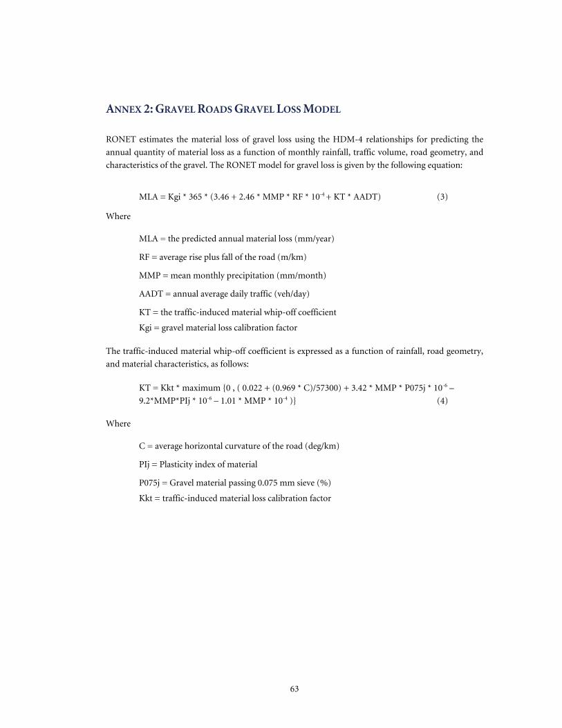
63

ANNEX 2: GRAVEL ROADS GRAVEL LOSS MODEL

RONET estimates the material loss of gravel loss using the HDM-4 relationships for predicting the

annual quantity of material loss as a function of monthly rainfall, traffic volume, road geometry, and

characteristics of the gravel. The RONET model for gravel loss is given by the following equation:

MLA = Kgi * 365 * (3.46 + 2.46 * MMP * RF * 10-4 + KT * AADT) (3)

Where

MLA = the predicted annual material loss (mm/year)

RF = average rise plus fall of the road (m/km)

MMP = mean monthly precipitation (mm/month)

AADT = annual average daily traffic (veh/day)

KT = the traffic-induced material whip-off coefficient

Kgi = gravel material loss calibration factor The traffic-induced material whip-off coefficient is expressed as a function of rainfall, road geometry,

and material characteristics, as follows:

KT = Kkt * maximum {0 , ( 0.022 + (0.969 * C)/57300) + 3.42 * MMP * P075j * 10-6 –

9.2*MMP*PIj * 10-6 – 1.01 * MMP * 10-4 )} (4)

Where

C = average horizontal curvature of the road (deg/km)

PIj = Plasticity index of material

P075j = Gravel material passing 0.075 mm sieve (%)

Kkt = traffic-induced material loss calibration factor

64

ANNEX 3: ROAD WORKS EFFECTS

RONET estimates the road works effects using the HDM-4 relationships that are given below.

Reseal

The roughness after a reseal is computed by the following equation.

RIaw = RIbw – maximum (0 , minimum (0.3 * (RIbw - 5.4), 0.5) ) (5) Where

RIaw = Roughness after reseal (IRI, m/km) RIbw = Roughness before reseal (IRI, m/km)

The structural number after a reseal is computed by the following equation.

SNaw = SNbw +REth * 0.2 * 0.0394 (6) Where

SNaw = Structural number after reseal SNbw = Structural number before reseal REth = Reseal thickness (mm)

Overlay

The roughness after an overlay is computed by the following equation.

RIaw = 2.0 +0.01 * maximum (0, (RIap - 2.0) * maximum (0 , (80 - OVth)) (7)

Where

RIaw = Roughness after overlay (IRI, m/km)

RIbw = Roughness before overlay (IRI, m/km)

OVth = Overlay thickness (mm) The structural number after a reseal is computed by the following equation.

SNaw = SNbw +OVth * 0.4 * 0.0394 (8)

SNaw = Structural number after overlay

SNbw = Structural number before overlay

65

Reconstruction

The roughness and the structural number of paved roads after a reconstruction is user defined at the

Country Data page.

Gravel Thickness

The gravel thickness after regraveling is computed by the following equation.

GTaw = GTbw + GTth (9) Where

GTaw = Gravel thickness after regraveling (mm)

GTbw = Gravel thickness before regraveling (mm)

GTth = Regraveling thickness (mm)

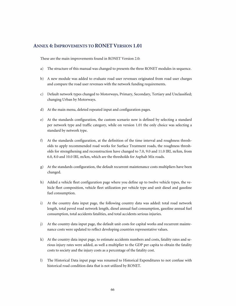
66

ANNEX 4: IMPROVEMENTS TO RONET VERSION 1.01

These are the main improvements found in RONET Version 2.0:

a) The structure of this manual was changed to presents the three RONET modules in sequence.

b) A new module was added to evaluate road user revenues originated from road user charges

and compare the road user revenues with the network funding requirements.

c) Default network types changed to Motorways, Primary, Secondary, Tertiary and Unclassified;

changing Urban by Motorways.

d) At the main menu, deleted repeated input and configuration pages.

e) At the standards configuration, the custom scenario now is defined by selecting a standard

per network type and traffic category, while on version 1.01 the only choice was selecting a

standard by network type.

f) At the standards configuration, at the definition of the time interval and roughness thresh-

olds to apply recommended road works for Surface Treatment roads, the roughness thresh-

olds for strengthening and reconstruction have changed to 7.0, 9.0 and 11.0 IRI, m/km, from

6.0, 8.0 and 10.0 IRI, m/km, which are the thresholds for Asphalt Mix roads.

g) At the standards configuration, the default recurrent maintenance costs multipliers have been

changed.

h) Added a vehicle fleet configuration page where you define up to twelve vehicle types, the ve-

hicle fleet composition, vehicle fleet utilization per vehicle type and unit diesel and gasoline

fuel consumption.

i) At the country data input page, the following country data was added: total road network

length, total paved road network length, diesel annual fuel consumption, gasoline annual fuel

consumption, total accidents fatalities, and total accidents serious injuries.

j) At the country data input page, the default unit costs for capital works and recurrent mainte-

nance costs were updated to reflect developing countries representative values.

k) At the country data input page, to estimate accidents numbers and costs, fatality rates and se-

rious injury rates were added, as well a multiplier to the GDP per capita to obtain the fatality

costs to society and the injury costs as a percentage of the fatality cost.

l) The Historical Data input page was renamed to Historical Expenditures to not confuse with

historical road condition data that is not utilized by RONET.

67

m) At the Monitoring Indicators output page, RONET is now presenting network safety indica-

tors in terms of fatalities and serious injuries.

n) At the Monitoring Indicators output page, RONET is now presenting an indicator for road

access that computes the all-weather roads area of influence (assuming a 4 km wide width

multiplied by the road length) as a share of the Country land area.

o) At the Performance Assessment module, the results are now being presented per budget sce-

nario and not per road work standard. There are three possible ways of defining the budget

scenarios: (i) evaluate optimal standard (lower society costs) per road class and lower and

higher budget scenarios; (ii) evaluate custom standard per road class and lower and higher

budget scenarios; and (iii) evaluate all road classes with the same standard (similar to version

1.01). The choice is done at the standards configuration page.

p) At the Network Performance output page, two new charts are being presented at the top of

the table: (i) the present value of road agency, road users, and total society costs for each

budget scenario, and (ii) the present value of net benefits of each budget scenario against the

present value of road agency costs.

q) The new Annual Work Program output page presents, for a user-defined budget scenario and

network, annual values for: (i) road agency, road user and total society costs, (ii) net benefits

compared to the Do Minimum scenario, (iii) asset value, (iv) road works length, and (v) av-

erage network roughness.

r) The new Solution Catalog output page presents, for a user-defined budget scenario, the stan-

dard that RONET selected for each road class for the given budget scenario.

s) At the Road Works Distribution output page, RONET is now calculating the Road Works

Costs per Vehicle-Km ($/veh-km).

t) At the Road Works Summary output page, RONET is now presenting a table with afforda-

bility indicators.

u) The speed of the calculation of the performance assessment module was improved.

69

References

1. Sub-Saharan Africa Transport Policy Program

http://www.worldbank.org/afr/ssatp

2. Highway Development and Management Model (HDM-4)

http://www.hdmglobal.com/

3. Road User Charges Model Version 3.0

http://www.worldbank.org/roadsoftwaretools/

4. Performance Assessment Model Version 1.0

http://go.worldbank.org/2VD3CR0LB0

5. Road Costs Knowledge System (ROCKS)

http://www.worldbank.org/roadsoftwaretools/

6. Road User Costs Knowledge System (RUCKS)

http://www.worldbank.org/roadsoftwaretools/

7. Highway Design and Maintenance Standards Model (HDM-III)

http://www.worldbank.org/roadsoftwaretools/

8. The True Cost of Road Crashes, Valuing Life and the Cost of a Serious Injury, International Road

Assessment Programme (iRAP)

http://www.irap.net/library.asp/

9. Rural Access Index: A Key Development Indicator, World Bank Transport Paper 10.

http://go.worldbank.org/EYOZ8CRSJ0