Use of Statistical Techniques for Sampling Inspection in the Oil and Gas Industry

Sieger TERPSTRA, Shell Global Solutions International B.V., Amsterdam, The Netherlands

Abstract. An overview is given of issues associated with the use of statistical tools, for sampling inspection applied in the Oil & Gas industry. Extreme value analysis is a well-known statistical approach. It is applicable to objects that have measurable damage. Less well known is the sampling inspection on objects where damage is not (yet) measurable, the so-called compliance sampling. Both schemes require care to prepare the inspection as they face the user with some hard to answer questions when it comes to design of the inspection, and analysis of the level of confidence obtained from a sampling inspection. Further complexity is added when a sampling inspection is carried out with a non-destructive testing technique, and the user has to select a technique with a proper detection threshold and an adequate sizing accuracy.

In this presentation the main properties of the sampling schemes will be discussed, and areas will be identified that impact on the applicability of the sampling schemes. There are certainly some issues with the statistical methods that inhibit their use in the inspection process. It is in the interest of the O&G industry to find optimal ways to address these issues. An essential first step is to develop a clear description of the most relevant ones, to develop a clear view how, where and by whom the statistical tools will be utilized, and by ranking the issues in terms of their importance for the business.

Introduction

1.1 What is sampling inspection

Integrity management of oil and gas production facilities and refining and chemical processing plant is a vital part of the business. In-service inspection plays a key role in that process, to verify and demonstrate that the actual condition of the pressure envelope and supporting structures is acceptable. For a significant proportion of such inspections a sampling inspection approach is applied.

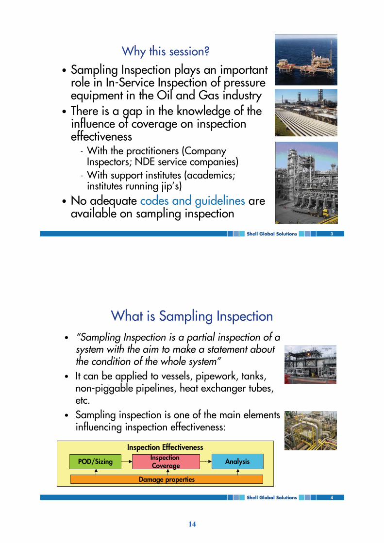
Sampling inspection is defined as a partial inspection of a system, for instance a vessel or a section of pipework, with the aim to extrapolate the results of the inspection to the un-inspected part, and making a statement about the condition of the complete system.

When a sampling inspection approach is applied to industrial plant two stages in the inspection process are of particular relevance: (a) the planning of the inspection and (b) the analysis of the result. The planning stage is concerned with, for instance, establishing the portion of the system to be inspected, the pattern of inspection coverage, and the required threshold for detection of damage and the sizing accuracy. During analysis the condition of the system is estimated, so that the next inspection can be planned, or remedial action to be identified (such as further inspection, repair or replacement).

4th European-American Workshop on Reliability of NDE - We.2.A.1

1

ww

w.ndt.net/index.php?id=

8315

Guidance for implementing a sampling inspection approach is to a limited extent available for some applications, in the form of industry standards or best practice guidelines. They typically provide rule-based instructions, and are applicable to relatively simple inspection conditions. For inspection problems with a higher complexity the use of statistical methods is indispensable. However, there are limited guidelines available in industry that provide the practitioners in inspection and NDE with suitable instructions.

This paper will explore the typical needs of the Oil and Gas industry for statistical tools, will highlight experiences with the implementation of such tools, address some of the problems experienced with their implementation, and indicate where gaps are present in the current tool box, and what could be done about these gaps.

1.2 Importance of sampling inspection

There are many objects that obtain 100% coverage during inspection; an example is in-line inspection of pipelines by intelligent pigs, and major vessels, reactors and storage tanks. However, there is also a large group of objects that normally obtains partial inspection, for instance justified by the fact that damage is of a local nature and occurring in preferred, predictable locations, that damage is only of a mild severity level, that a component is not completely accessible for inspection, or that only a short time interval needs to be bridged to a next, full, inspection. Pipework is traditionally inspected with a sampling approach, which is reflected in industry codes and standards. Pressure equipment (vessels, reactors), tanks and heat exchanger bundles are increasingly subject to sampling inspection, particularly when a non-intrusive inspection approach is applied to replace an internal visual inspection.

Sampling inspection is an important means to realize an acceptable cost level for inspection. It can be perfectly adequate, when based on sound experience and proper risk based assessments; at the same time the consequences of having it wrong can lead to a failure of the pressure envelope or a failing support structure, with significant consequences. This requires that those responsible for implementing a sampling inspection approach do understand its nature and its performance.

1.3 Is the performance of sampling inspection well understood?

For an inspection engineer, the use of a sampling inspection approach is probably the most complex element of the inspection process. Clear guidelines are often lacking, and are of a simplistic nature at the most. A pre-requisite for setting up a proper sampling inspection approach is an intimate knowledge of the degradation mechanisms in the plant. A gut feel for sampling principles is often the basis for making an inspection plan and interpreting the results. In that respect many years of experience help to develop an intuitive feel for the statistical elements that play a role in a sampling inspection approach.

However, this level of understanding puts strain on the inspector and on the inspection planning systems, as current operation of installations has moved the inspection process away from the comfort zone, in which experience may have played a large role; a pro-active approach to the integrity management process, including inspection, is required nowadays, due to a multitude of factors: • Use of a diverse range of materials, with a diverse range of damage mechanisms; • More complex operation of plant, with more variation in operating conditions, and a

higher impact of failures; • Legislation allowing self-regulation, but at the same time requiring adequate

demonstration of inspection performance;

2

• An ongoing effort to reduce the cost-impact of inspection on operations, for instance by making use of non-intrusive inspection replacing internal visual inspection of vessels, by utilizing permanently installed monitoring tools, and for certain type of operation the realization of minimum intervention maintenance an inspection philosophies.

Industry has developed many initiatives that have contributed to - an improved understanding of - the effectiveness of the inspection process, such as the use of Risk Based Inspection methods, the development of guidelines for non-intrusive inspection, an ever developing capability of NDE methods, a continuous effort by the industry to demonstrate the reliability of NDE tools and to demonstrate the effectiveness of the inspection processes as a whole, and an increasing awareness in industry to apply qualification methods to demonstrate adequate performance of NDE tools as well as inspection strategies.

However, in the above developments one aspect of the inspection process is significantly under-represented: the influence of a sample inspection strategy on the overall effectiveness of the inspection process. Sampling inspection is not covered well in the guidelines and rule sets of risk-based inspection planning tools, is only partly addressed in some non-intrusive inspection projects, not part of NDE reliability models (POD Generators), not included in NDE performance demonstration programs, not included in inspection validation guidelines, and only partially covered in industry guidelines. Moreover, coverage of the subject in major NDE conferences is minimal.

The above gap-list of does not mean that our industry is devoid of knowledge of statistical methods required for sampling inspection. The principles of basic statistical methods are in use for decades, and the first applications of Extreme Value Analysis date back to the 1950’s; statistical engineers employed inside and outside oil companies often get involved in solving inspection problems; complex statistical models are being developed in other disciplines (such as maintenance), which appear remarkably suitable for inspection as well.

To understand which type of efforts are needed to close the gap on the underdeveloped role of sampling inspection it is important that we understand the factors that have retarded its development. There are very relevant learning points to be taken from past experiences with the implementation of sampling recipes. There are also important lessons to be taken from other development processes in industry, notably the joint industry efforts to improve inspection reliability, with development of POD Generators, NDE performance demonstration programs, common guidelines for inspection qualification, etc.

In the further part of this paper we will first zoom in onto the main statistical recipes relevant for sampling inspection, and then show what gaps there are and how certain factors inhibit the smooth implementation of statistical methods in inspection. This then provides a starting point for an action program for industry to close gaps.

2. Properties of sampling inspection methods

In this section the two main statistical recipes are introduced.

2.1 Extreme Value Analysis

Extreme Value Analysis is the most well known statistical method to analyse inspection data. There is a vast amount of literature covering its application, also to in-service inspection problems in the Oil and Gas industry.

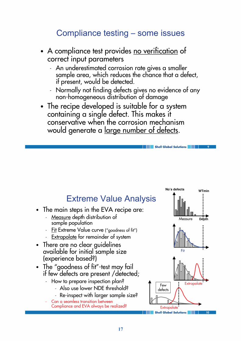
As a most brief description, an Extreme Value Analysis approach takes inspection data from a sample area sub-divided in small sub-sections, fits a distribution to the observed damage parameter (typically the largest depth or length of the damage as measured in the sub-sections), and then extrapolates the distribution to obtain an extreme

3

value distribution from which the most likely maximum depth or length (the ‘extreme value’) can be derived that can be expected somewhere in the whole system. Details of the extreme value analysis method are elaborated upon in a separate paper in this conference [1].

An important pre-requisite for extreme value analysis is that it only works if actual damage is detected; otherwise the statistical method is not working. Also, the damage needs to be found in sufficient quantities; otherwise the accuracy with which the extreme value is determined may not be sufficient to prove that the component is fit for service. This important pre-requisite makes that the Extreme Value Analysis method is not effective for many conditions where sampling inspection is applied; it requires another statistical method, which is discussed below.

2.2 Compliance testing

There are many conditions in which it is likely that during inspection no damage will be detected (see next section). Compliance testing is now applicable as the statistical method. This type of statistics is well known from quality testing in production / fabrication, and is for instance also applied in programs to demonstrate the performance of NDE tools (compliance testing is a special case of acceptance testing, for which no defective units are acceptable). Two variants are discussed here, a simple scheme that tests on the presence of defective units and a more advanced scheme that provides a test on the allowable depth of a defect.

A most brief description of the two schemes is given below. More details can be found in a separate paper in this conference [2].

Testing for defective units: From a group of items (welds; sections of pipe) a certain number (the sample size) is inspected, and each item is evaluated against an accept/reject criterion. When not finding a defective unit in the sample the inspection has demonstrated, with a certain level of confidence that the whole group of items contains less than a certain proportion p of defective units.

Testing for a maximum defect size: From an area that may contain a single defect of a group of defects a sample area is inspected. The sample size is determined by the probability that a defect with a ‘critical’ size could be present, and by the required confidence level that the inspection is successful. If during inspection of the sample no defect of any size is detected it can be stated, with the given confidence, that the whole area does not contain a defect with a critical size. Note that in this scheme it is assumed that the inspection technique has a sufficiently low threshold that it is capable to detect a significant proportion of the defect population (see also the section on ‘statistical recipes and the phases in the life cycle’).

There are some marked differences between the above two recipes; the first recipe provides an answer in terms of the proportion of defective units. This recipe is for instance suitable to demonstrate the absence of unacceptable defects such as stress corrosion cracks. However, the recipe does not score very well on a very important property, namely the required sample size to demonstrate the absence of unacceptable defects: when only a few defective units are expected in the system then an almost 100% coverage is required, while only obtaining a moderate level of confidence. This creates an issue that is more extensively discussed in the section on ‘Understanding the effect of the number of defects’.

The second recipe provides an output related to the depth of the defects; this is very practical, as the recipe can then be used to demonstrate a minimum value for the remnant life of components (because the depth of corrosion defects and knowledge of the growth rates one is able to estimate the remnant life).

4

Although each of the recipes are intuitively logic, and can be explained to statistical laymen (like inspection engineers), it requires quite some familiarization with the underlying principles of the recipes to be able to work with them independently, and be able to judge whether a recipe is applicable to a particular inspection problem, or whether certain factors could jeopardize the reliability of the sampling inspection approach. Some major aspects are discussed in the next two sections.

3. Applicability of statistical sampling recipes

Several important parameters play a role in the applicability of statistical methods for sampling inspection. Some parameters play a trivial role and can therefore help to develop simple application rules (see for instance ‘life cycle’ below). Other parameters may affect applicability over only part of the parameter range, while being difficult to predict (see for instance ‘number of defects’).

In all cases a statistical recipe requires quantitative input (such as a maximum allowable defect size, a probability of the presence of unacceptable defects, a required statistical confidence in the test). The basis for such quantitative information is best found in a Risk Based Inspection system, as that contains detailed information on the components that are subject to inspection.

The functional requirements of RBI systems may have to be adapted, so that they fully support the input requirements and analysis capability that is required for the use of a sampling inspection.

3.1 Statistical recipes and phases in the life cycle

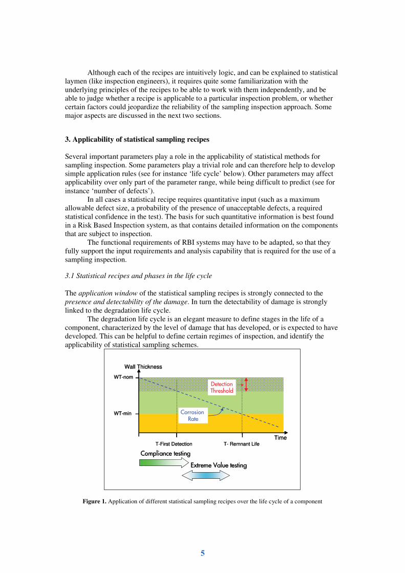
The application window of the statistical sampling recipes is strongly connected to the presence and detectability of the damage. In turn the detectability of damage is strongly linked to the degradation life cycle.

The degradation life cycle is an elegant measure to define stages in the life of a component, characterized by the level of damage that has developed, or is expected to have developed. This can be helpful to define certain regimes of inspection, and identify the applicability of statistical sampling schemes.

Wall Thickness

WT-min

WT-nom

Time

������������ ����

����� �������

T-First Detection T- Remnant Life

������������ ����

�������������� ����

Wall Thickness

WT-min

WT-nom

Time

������������ ����

����� �������

T-First Detection T- Remnant Life

������������ ����

�������������� ����

Figure 1. Application of different statistical sampling recipes over the life cycle of a component

5

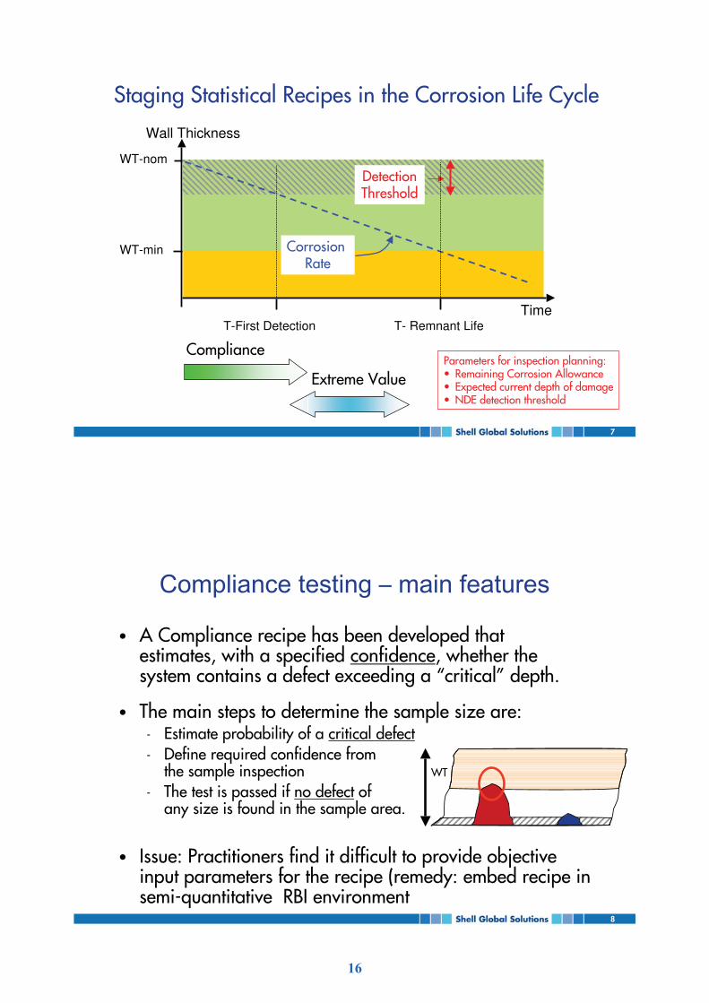
In Figure 1 a simple remnant life plot is shown of a component that is subject to a constant degradation rate, starting from day 1 onwards. Several important stages can be illustrated with the plot: • When the corrosion has progressed to the point that the minimum wall thickness has

been reached the corrosion life is actually consumed; any associated defects become unacceptable, and the component needs repair or replacement.

• When the component is inspected a blind zone will be present (every inspection technique has a threshold below which no defects are detected).

The application window of the statistical sampling recipes can be marked on the time axis of the remnant life plot. Several start- and end-points can be given based on qualitative facts: • Compliance testing can be applied from day 1 onwards; • Compliance testing will fail when defects have grown to a detectable size; • Extreme value testing starts to become effective when damage has grown to a

detectable level; • Extreme Value testing will increasingly fail to demonstrate the absence of

unacceptable1 defects when defects approach the minimum wall thickness. For inspection planning one has to quantify the application range over which these recipes are effective, by calculating component-specific input parameters as required by the statistical recipes. This is not trivial and is an issue that is further discussed in section ‘embedding statistical recipes in RBI software’.

3.2 Understanding the effect of the number of defects

The number of defect that can be detected during sampling inspection has a significant influence on the effectiveness of a statistical scheme for sampling inspection. In some circumstances it is more trivial than in others, but its influence can be so strong that the correct estimate of the number of defects detected can dominate the overall confidence in the inspection result, or create a large uncertainty in the planning phase of an inspection. A few situations are highlighted: 1. Sufficient defects must be detected for an Extreme Value Analysis to accurately fit a

distribution to the measured population. If too few defects are present the statistical uncertainty in the resulting extreme value will increase; although it may still represent an acceptable defect size, a large uncertainty band may not be good enough for a critical inspection. The consequence can be that the inspection is ineffective, and needs to be extended, or repeated with other tools (more sensitive). In some parts of the business such uncertainty in the planning of an inspection cannot easily be accommodated, making sampling inspection a less attractive inspection approach. o Tools are required that provide support to the inspector during planning of

inspections, showing the impact of defect density. A link to relevant properties of the NDE systems (such as detection threshold) must be made transparent.

2. When applying compliance testing one can intuitively see that a large density of defects will lead to a high chance that a defect is detected, even when a small area is sampled. It means that a compliance scheme is effective for such conditions in correctly rejecting a system with unacceptable damage.

3. It is more difficult to obtain confidence from a compliance scheme when a system is inspected that that is actually in good condition. This is particularly so when a

1 The acceptable size of defects during inspection is a different value than the size related to the minimum wall thickness; acceptable size during inspection must be less otherwise the inspection is not capable to demonstrate a positive remnant life after inspection.

6

degradation mechanism may be active (i.e. would be capable to generate severe defects) but only in a small number of locations. o The compliance recipe currently in use takes account of the possibility of isolated

defects; this makes the recipe very conservative for conditions where numerous defects are potentially produced.

o A compliance test will normally not provide evidence of the density of a defect population as damage is still small or absent (see also the section ‘compliance scheme - circular problem’).

o A remedy for the impact of unknown density is not trivial; most likely it has to come from knowledge of the typical degradation characteristics, either coming from experience or from the knowledge of corrosion mechanisms.

The effect of density of defects on the application window of the sampling recipes over the life cycle of a component is summarized as follows: 1. For systems with a large density of defects a smooth transition is likely from

compliance testing into extreme value testing. 2. For systems with a low density of defects compliance sampling may have to be

followed by an inspection with 100% coverage. This may already happen very early in the life of the system, dependent on the uncertainty in the predicted corrosion rate. a. When a 100% inspection is carried out with a very low detection threshold (for

instance an internal visual inspection under well prepared surface and access conditions, or when an effective assessment of an internal coating can be established), and no defects are present, this would reset the system back to the original condition. A next inspection can then be based on sampling inspection again.

b. If upon 100% inspection some localized defects would be detected, these could be separated in a separate stratum, and the remainder of the component it could again be inspected with a sampling approach.

3.3 Input to a compliance test – a circular problem?

It has been shown in an earlier section that a compliance recipe may require, as an input during planning, an estimation of the ‘probability of a critical defect’. This is due to the fact that the underlying statistical framework is using a Bayesian scheme; this requires an estimate of the defect depth before inspection (prior depth), which is combined with a measured depth, giving an updated, posterior, depth.

When introducing such a scheme in the mid-nineties in the author’s company, it appeared that this created too much a challenge for the users, due to the absence of a reliable estimate of the ‘probability of a critical defect’.

In a separate paper it is shown how the recipe has been embedded in the Risk Based Inspection planning system, to provide support to the user to generate more objective input data. By the nature of the underlying inspection model the sample size calculated by the recipe is entirely determined by the remnant life parameters (remaining corrosion allowance; future corrosion rate). This shifts the problem away from the subjective and case-by-case assessment of the inspector/corrosion engineer towards the reliability of the inspection and corrosion data present in the RBI database.

To allow the inspector to exercise control on the reliability of the inspection sampling approach it is recommended that additional tools are made available to carry out a reliability assessment of the inspection parameters, so that an assessment can be made of the robustness of the sampling scheme.

7

3.4 Result of a compliance sample inspection – verifiable?

It has been shown in an earlier section that, during planning, a compliance recipe may require as an input an estimation of the ‘probability of a critical defect’. This is one of the two major governing parameters determining the sample size. Normally, the result of a compliance test will not show any defects. This has the consequence that the inspection is not providing effective confirmation that the original parameters were correctly estimated.

One can easily imagine the following loophole: by underestimating the estimated corrosion rate prior to inspection, an inspection with a small sample size would be considered to be adequate. However, a small sample size is not very powerful is detecting unfavourable (misjudged) conditions, such as unevenly distributed defects, or a system with a few defects of which the actual depth has been under estimated.

This emphasizes the importance of having reliable corrosion rates available. To reduce the impact of this weakness it is recommended that an inspector is not

only provided with a recipe that allows calculation of inspection sampling size but has additional tools available to carry out a sensitivity analysis on the input parameters to be able to assess the robustness of the sampling scheme.

3.5 Embedding statistical recipes in RBI software

A compliance scheme leads to a relatively simple inspection process (sample size is determined; area/components are examined; normally minimal analysis is required as no damage is expected; a simple report results). However, to ensure that an acceptable level of confidence in the inspection result will be obtained requires quite an effort: • Defects grow over time, changing the inputs into the sampling scheme, requiring a

calculation of sample size for each individual inspection. • Defect size is assessed relative to the local corrosion allowance; this may require the

use of different sampling sizes per component. • The sample size calculation is highly non-linear; in combination with the wide range of

the input parameters it is virtually impossible to generate simple tables for inspection sample sizes, except for the very simplest of cases (a condition very early in the life cycle, i.e. non-corrosive services). The latter provides a much too limited scope.

• To ensure that an NDE technique is applied that is actually capable to detect a sufficient proportion of the defect population, a calculation of the required detection threshold of the technique is required.

It is strongly recommended that the use of statistical recipes be supported with software connected to the inspection database. This allows, on the one hand, meaningful sampling parameters to be calculated, while taking away the complexity of calculations across the multiple input parameters, and allows on the other hand the necessary checks to be carried out to ensure that reliable and meaningful data has been used as input to the schemes.

4. Factors that can spoil sampling inspection

There are factors that may cause the sampling inspection approach to fail. In certain conditions these factors are observable so that some level of testing could be applied to validate the sampling inspection scheme, but in other conditions the effects are hidden.

8

4.1 Non-homogeneous distribution of damage

A pre-requisite for a statistical method to work is that the random variable that is measured (such as the wall loss) is a truly random variable, across the whole system that is subject to a sampling inspection approach. A requirement of this kind is often preceding the recipe, as a sort of disclaimer. This poses a problem to the inspector and corrosion engineer to understand whether the damage inspected for is behaving as such. Quite often it is even known that the location where corrosion damage occurs is not so much random, but unpredictable, due to a multitude of parameters that may be active; with detailed knowledge of the conditions of flow, fouling, condensation, etc, the corrosion pattern may not look that random anymore.

In this area there is a lack of understanding whether and when the effect of a non-homogeneous distribution of damage will jeopardize the accuracy or even the validity of the statistical method.

This problem is manifesting itself at different levels: • On a macro-level large systems like a corrosion loop or a vessel are supposed to be

subject to a similar corrosion environment, but when taking a closer look they are often subject to significantly different conditions, for instance due to differences in flow, gas/liquid phase, etc. This requires that the system has to be divided into corrosion strata within which the damage is of a sufficiently homogeneous nature. o For extreme value analysis an initial sample size is required. There are no clear

rules to set this initial size, and by its nature of the method, adequate sample size is only becoming clear once the data is analysed (e.g. when it shows an adequate goodness of fit test result). One can easily imagine that small, local corrosion strata with a different level of damage could lie outside the sample area inspected; if the results from the sampled area show a good fit the inspection result may be considered to be acceptable, while in fact the result is not representative for the whole system. A solution to this potential loophole is to differentiate the required initial sample size, and make it dependent on the expectation of the level of homogeneity of the damage: less homogeneous distributions of damage would require a larger initial sample size. Such a requirement could be based on knowledge of the degradation mechanism or based on experience with particular operating conditions. Such experience-based criteria have to be provided via application guidelines, specific for certain production plant and process conditions.

o In case different strata are expected in a system, methods are required that allows a user to set up an inspection scheme that provides assurance (in the planning phase) that each stratum is inspected with the right sample size, and will help to verify (in the analysis phase) that the correct stratification has been applied.

o It is noted that this works out differently for compliance testing and extreme value testing: When using a compliance scheme the verification of stratification is yet not possible, as damage has not developed into measurable patterns. Therefore a tool should allow sensitivity tests to be carried out to determine whether a sampling scheme is robust against a wrong assessment of the corrosion strata.

• On the mesa-level another conflict with a pre-requisite of statistical methods can occur: when collecting data for an extreme value analysis the minimum values measured in the sub-sections in the sampling area (the so-called block size) are supposed to be independent. However, it is not uncommon that clustering of damage may occur due to locally more severe conditions, e.g. as a result of deposits, pools of fluids, impact conditions. This may cause the random defect depth to have a certain level of dependency, which may cause the statistics to break down.

9

o On this subject more knowledge would be required to understand the effects, and to obtain criteria for estimating when measures have to be taken to reduce the effect dependent data (choosing block size; de-clustering the data).

4.2 Multiple corrosion histories

It is common for equipment and piping in a plant that it has seen different operating conditions over time. This may cause a mix of historic and current damage, which all ends up in the same depth distribution.

Better knowledge is required to understand when a mix of corrosion damage histories may interfere and make the statistical analysis invalid. A way to develop such knowledge may be via the use of simulation models as well as the collection of field experiences. More stringent assessment criteria should be developed for conditions where a mix of corrosion histories is likely. Additional inspection tasks may then be recommended to evaluate such multiple corrosion conditions. Monitoring may be one way to differentiate between active and dormant parts of the damage.

4.3 False calls and accuracy – optimizing NDE tools

A characteristic of sampling inspection is that the NDE results are used in a much more quantitative manner than NDE practitioners are used to in most of their day-to-day life. It may happen that the effects of the NDE performance become clear during the analysis phase, in the form of large statistical uncertainty as a result of too large measurement errors or the presence of false calls. In ultrasonic corrosion mapping the presence of responses of plate inclusions is notorious; to rescue the inspection results a laborious data cleansing action may be the result.

It is recommended that tools are made available that allow an assessment of the NDE requirements with respect to false calls and measurement accuracy; this would probably combine easily with requirements for detection threshold needed in another stage of the inspection planning. Probability of detection is expected to play a less important role in many cases, but probably needs inclusion when defect numbers are low and may lead to inaccurate results due to statistical noise.

4.4 Using the correct statistical variable

Pipework inspection is, by its nature, done with NDE tools and is, in most cases, carried out with a sampling approach. Traditional pipework is divided in corrosion loops that are subject to a similar corrosion environment; inspection is done at so-called corrosion measurement locations. Wall thickness is measured at certain intervals, and replacement is initiated when sections of pipework reach the minimum required thickness. This approach works well in pipework of a uniform design, and when corrosion rates, and the pattern in which the corrosion develops, are rather stable over time and in place.

The planning of pipework inspection becomes more challenging if it is build from many different diameters and thicknesses, and if it has developed a mature corrosion condition that requires regular replacement of sections of pipework.

To obtain an overview of corrosion behaviour in the whole system, the measured wall thickness or the remaining corrosion allowance of individual pipe sections may not provide an accurate estimate of the typical corrosion rate in the system, unless the pipework that has a uniform build (same thickness and same corrosion allowance). In larger systems the nominal thickness can vary significantly, and also the corrosion allowance would vary if a fitness for service level would be used, slightly more than the design corrosion allowance.

10

By converting wall thickness into wall loss one obtains a much more effective parameter to reveal the corrosion behaviour across the whole corrosion loop. As the measurements are often spread out over time, in irregular intervals, a conversion of wall loss into corrosion rate removes the time factor and allows comparison of local inspection data.

It has been shown that the step from analyzing thickness data to analyzing wall loss and corrosion rate data has several benefits: • Wall loss, unlike wall thickness, is a statistical variable that is not contaminated with

pipe design factors; • Comparing wall loss data over a relatively large system (instead of a small section of

pipework of uniform design) enhances the statistical accuracy when analyzing corrosion behaviour;

• The conversion of thickness data into wall loss and corrosion rate will allow the application of a pure risk-based inspection approach.

How such a pipework inspection approach works out is described in a separate paper [3].

5. Validation of sampling inspection strategies

Sampling inspection is an important step in the inspection process that can have a significant impact on the effectiveness of an inspection. Therefore it is vital that the methods and guidelines used for sampling inspection are adequately validated, so that a reasonably uniform performance across industry is obtained, which in turn will raise acceptance by equipment owners and regulators, when sampling inspection is part of, for instance, critical non-intrusive inspection applications.

It is suggested to distinguish several levels of validation: • Validation of the tools, such as the statistical methods used.

There are variants of certain statistical methods, which should be compared on their technical merits. Examples are variants of the extreme value analysis method; tools used to distinguish different corrosion strata; tools that identify and subsequently reduce the effect of clustering and dependency in the data. A possible approach for this validation could be the comparison, in a joint industry effort, of different statistical tools applied to the same reference data set.

• Validation of application guidelines. The use of statistical tools has to be embedded in the inspection work process, which will provide instructions on various detailed aspects (for instance the selection of a particular statistical method for a specific inspection problem), and the use of acceptance criteria. Examples of such criteria are for instance the acceptance level for a goodness of fit-test in an extreme value analysis that tells the user that the data is suitable for extrapolation; or the use of a certain upper bound confidence level for the extreme value (e.g. 80% or 95%). Validation of the instructions in the guideline should reveal whether the statistical method provides a robust application window, to ensure that the sampling inspection approach will have an adequate level of conservatism. This type of validation is probably more complex, as one is interested not in the average performance of the statistical method but in its performance when the properties of the measured corrosion damage might not be ideal anymore. More on this subject is discussed in another paper in this conference [4].

11

6. A future agenda

The development of Industry Guidelines describing proven statistical methods is expected to support several shortcomings in this area: • Closing the gap on the poorly quantified effect of sampling inspection on overall

inspection effectiveness. • Enhancing the acceptance of sampling inspection by users and regulators. • Enabling the sharing information on performance of sampling inspection. • Enabling joint industry efforts to validate the performance of sampling inspection

strategies. The sharing of methods and experiences will allow a streamlining of contributions from various parties: • Inspection and corrosion engineers sharing the prediction of the properties of defect

distributions. • Inspection and statistical engineers to develop non-standard statistical approaches,

beyond those in the guideline. • NDE service companies and inspection engineers to tune the NDE performance to the

need of the sampling problem. • IT engineers to provide the necessary tools in the Inspection Management database. Further development of statistical methods for inspection is required from where they currently are, so that they become versatile enough to handle the complexity of real-world inspection cases. In addition to the recipes that calculate sample size for various types of inspection problems and tools for extreme value analysis, it also requires additional tools to assess the effect of non-homogeneous behaviour of defects or of measurement errors and artefacts. Moreover, tools are required to allow a sensitivity analysis on the robustness of a sampling scheme. Parties that can contribute to such development are: • Statistics groups in academic centres. • Research institutes on NDE and inspection. • Joint industry programs (development and validation of methods). • Standardization committees.

References

[1] Application of Extreme Value Analysis to Corrosion Mapping Data, C. Schneider, C. Bird, 4th European-American Workshop on Reliability of NDE, Berlin, 24-26 June 2009 [2] Implementation of Compliance Sampling using RBI Parameters for Partial Equipment Inspection P. van de Camp, F. Hoeve, A. Ostrowska, S. Terpstra, 4th European-American Workshop on Reliability of NDE, Berlin, 24-26 June 2009 [3] Tools and Methodologies for Pipework Inspection Data Analysis, P. van de Camp, F. Hoeve, S. Terpstra, 4th European-American Workshop on Reliability of NDE, Berlin, 24-26 June 2009 [4] Wall Thickness Distributions for Steels in Corrosive Environments and Determination of Suitable Statistical Analysis Methods, M. Stone, 4th European-American Workshop on Reliability of NDE, Berlin, 24-26 June 2009

12

������������ ������������������� ����������������������

�������������

��� ���������� ���������������������������������� �����

!��"���#�����!�����$������!��������%������������� &'&��"��&������(����&)�*

�

+������

, ��������������!�*���"�%��)����, ������!�*���"�%��)������*������-, .����)���������!������)��� �)��

� +�*����)�������"� �/���*��'�����.�����

, %*��*������������, .����������"��0�

13

�

������������-, !�*���"�%��)�������������*���������������%��!��1�)��%��)���������������2��*�����������3�����0�$����0����

, #���������"������������4��0"����������������)�����)�1���"��������)���������)��1���

� �����������)���������5+�*����%��)���6�������1�)��)�*����7�

� �������������������5�)�0�*�)6����������������"�8�97

, ����0�2�����)�0����0�"��0������������1������������*���"����)����

�

�������!�*���"�%��)����, ��������� �������� ������������ ������������

� ��������������������������� ��������������������������������������� � ����

, %��)����������0����1�������4����������������""�������������������/)���"�����������)&

, !�*���"����)������������������*�������*�����������)��"����)���������)��1���:�

������ �����������

���������� ������ ��� ���� ��������

�������� �����

14

%*�����)������*���"����)����

, %����4������ !�*���"����)�����������������������*������������������

�2��*����5�������4���76� ����%�����1��%��)�����5�%%7����1�������������)�����"�����

, #�������"�����*���"�*������)��)���"�� ;�0�����0��"���0�0�*��������"�����)��1����������)�������

��)�*��"�*�����*������:� <��������)����0�%��)�����������"���)�����"����������06� =�������>�����������/�)��������)�����"������0����������0�)����&

, %��)�����)�1���"��������"����)�����*�)������1������)��� 5)�����0��"6�������������*�1�����%%�1 %'%�?7

?:��%%�@�����%�����1��%��)����6�%'%�@�%��������1�����%��)����

!

.����)���������!������)��� �)��

#����������4��*����"�������������)�����)��:, �/���*��'�����.����� 5�'.7�, +�*����)�������" 5���"������:��))����)�������"7, #���*����0���������������:

� �'.���2�����0���)���������)�����)��������0�*�"�����*��������������)�����)���4���6�

� +�*����)�������"���*�����0�*�"��4�������0���)��0

, #�������4��������"������������)�����)�������"�4��������+��������A����+�)��:

15

"

!��"��"�!������)��� �)����������+��������A����+�)��

Wall Thickness

WT-min

WT-nom

Time

+�������� ���

T-First Detection T- Remnant Life

+�*����)�

����)�����#������0

�/���*��'����=���*������������)�����������":, �*�����"�+��������.���4��)�, �/�)��0�)�������0�������0�*�"�, ����0���)������������0

#

��������� �� ���� ������� ����

, .�+�*����)����)�����������0�1����0���������*�����4�������)����0�)����0��)���4��������������*�)���������0���)���/)��0��"���B)����)��C�0���&

, #���*����������0����*���������*����>�����:� ���*��������������������)����)���0���)�� ���������2����0�)����0��)�����*�

�����*������)����� #�����������0�������0���)� ���

�����>��������0���������*�������&

, %��:�=��)������������0����0����)���������1�0����8�)��1����������*���������������)���5��*�0�:��*��0���)�������*��2���������1��� %���1����*����

�#

16

$

��������� �� ���� �����������

, .�)�*����)��������1�0�����1�����)����� ���)����)����������*����� .����0�����*���0�)�������������"�1����*�������*���������4��)����0�)������)���)���������0���)�������������4���0����0���)��0&

� ���*������������0��"�0���)��"�1������1�0��)���������������*�"������0��������������0�*�"�

, #�����)���0�1����0��������������������*�)��������"�����"���0���)�&�#���*�������)����1���1��4��������)��������*�)����*�4���0�"�������������"����*�������0���)�&�

%&

�� ������������������

, #���*���������������'.���)������:� <����� 0����0��������������

�*������������ D�� �/���*��'�����)��1��5B"��0���������C7� �/�������� ������*���0���������*

, #������������)�����"��0�������1���������������������*����>��5�/�����)�����0-7

, #���B"��0���������C�����*������������4�0���)������������E0���)��06� F�4�������������)��������-�

� .��������4��������������0-� �����)��4�������"����*����>�-

� +�������*����������������4����+�*����)����0��'.���4�����������>�0-

WTminNo’s defects

<�����

D��

Depth

�/��������

�/��������

D�40���)�

17

%%

������� � ���� ������

, A������"�����:�#���������1������"��)�*��/�������������)�����)���5*��������*����6�)��0������0���0���7�)��������0���**�:� B<�����C��������*�����0���)�����0����)���� +����0��)������������)�*��*�����*������4������)�������4������������*�����������)������

, !�������:��*��0�������)�����)���������*��2���������1�� %�������"�0������� A�4���)�*��/�����������������*������0�2������01��)�0�*�0�������))������������������������*����

%�

!������"�������������)�

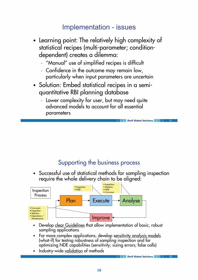
, !�))�����������������)���*����0������*���"����)�������2���������4�����0���1����)��������������"��0:

, ��1����)�����$��0����� ���������4��*��*���������������)���������*���"����)�����

, D���*����)�*��/����)�������0�1���������1�����������*�0��54������7����������"�������������*���"����)�������0��������*�>��"�����)����������5�����1���6��>��"������6������)���7

, %�0�����4�0��1���0����� ���*����0

=��� �/�)��� .�����

%*��1�

,+�������, %��)����, !������), 3��������E�<��������)�

, %��)����, ���

, %��)����, !������), ���, +�������%��)����

=��)�

18

%�

���� ����������

, #�����/������������������4����"�������*����0�������1��������8�)��5)�*����)�6��'.6���4���6�1���0�����7

, �����*��������2����0����0����������������)���:� ��1���*�������*����0� ��1���*�������5���4�����*�������7������ ��1���*�������"��0������ #������"���0����4��0"�������"�� '���0������������)�����

, G���������1���0��������)������������ ���������������������������1��4�����������������������������"��0�

������������ ������������������� ����������������������

�������������

#��������

19