United States Environmental Protection Agency

Demonstration of In Situ Dehalogenation of DNAPL through Injection of Emulsified Zero-Valent Iron at Launch Complex 34 in Cape Canaveral Air Force Station, Florida Innovative Technology Evaluation Report

EPA/540/R-07/006 September 2004

Demonstration of In Situ Dehalogenation of DNAPL through Injection of

Emulsified Zero-Valent Iron at Launch Complex 34 in

Cape Canaveral Air Force Station, Florida Final Innovative Technology Evaluation Report

Prepared by

Battelle 505 King Avenue

Columbus, OH 43201

Prepared for

U.S. Environmental Protection AgencyNational Risk Management Research Laboratory

Superfund Innovative Technology Evaluation Program 26 Martin Luther King Drive

Cincinnati, OH 45268

Foreword

The U.S. Environmental Protection Agency (EPA) is charged by Congress with protecting the Nation's land, air, and water resources. Under a mandate of national environmental laws, the Agency strives to formulate and implement actions leading to a compatible balance between human activities and the ability of natural systems to support and nurture life. To meet this mandate, EPA's research program is providing data and technical support for solving environmental problems today and building a science knowledge base necessary to manage our ecological resources wisely, understand how pollutants affect our health, and prevent or reduce environmental risks in the future.

The National Risk Management Research Laboratory (NRMRL) is the Agency's center for investigation of technological and management approaches for preventing and reducing risks from pollution that threaten human health and the environment. The focus of the Laboratory's research program is on methods and their cost-effectiveness for prevention and control of pollution to air, land, water, and subsurface resources; protection of water quality in public water systems; remediation of contaminated sites, sediments and ground water; prevention and control of indoor air pollution; and restoration of ecosystems. NRMRL collaborates with both public and private sector partners to foster technologies that reduce the cost of compliance and to anticipate emerging problems. NRMRL's research provides solutions to environmental problems by: developing and promoting technologies that protect and improve the environment; advancing scientific and engineering information to support regulatory and policy decisions; and providing the technical support and information transfer to ensure implementation of environmental regulations and strategies at the national, state, and community levels.

This publication has been produced as part of the Laboratory's strategic long-term research plan. It is published and made available by EPA's Office of Research and Development to assist the user community and to link researchers with their clients.

Sally Gutierrez, Director National Risk Management Research Laboratory

ii

Notice

The U.S. Environmental Protection Agency has funded the research described here­under. In no event shall either the United States Government or Battelle have any responsibility or liability for any consequences of any use, misuse, inability to use, or reliance on the information contained herein. Mention of corporation names, trade names, or commercial products does not constitute endorsement or recommendation for use of specific products.

iii

Acknowledgments

The Battelle staff who worked on this project include Arun Gavaskar (Project Man­ager), Woong-Sang Yoon, Megan Gaberell, Eric Drescher, Lydia Cumming, Joel Sminchak, Jim Hicks, Bruce Buxton, Michele Morara, Thomas Wilk, and Loretta Bahn.

Battelle would like to acknowledge the resources and technical support provided by several members of the project team:

• Tom Holdsworth and Ron Herrmann at U.S. EPA for providing resources to evaluate this demonstration.

• Jackie Quinn at NASA who provided technical guidance and oversight.

• Suzanne O’Hara, Thomas Krug, and David Bertrand from GeoSyntec Consultants.

• Cherie Geiger and Chris Klaussen from University of Central Florida.

• John DuPont and Scott Schroeder from DHL Analytical.

• Randy Robinson from Precision Sampling.

iv

Executive Summary

The purpose of this project was to evaluate the technical and cost performance of emulsified zero-valent iron (EZVI) technology when applied to DNAPL contaminants in the saturated zone. This demonstration was conducted at Launch Complex 34, Cape Canaveral Air Force Station, FL, where chlorinated volatile organic compounds (CVOCs), mainly trichloroethylene (TCE), are present in the subsurface as DNAPL. Smaller amounts of dichloroethylene (DCE) and vinyl chloride (VC) also are present as a result of the natural degradation of TCE.

The EZVI project was conducted under the National Aeronautics and Space Administration (NASA) Small Business Technology Transfer Research (STTR) Pro­gram. The Small Business Concern is GeoSyntec Consultants (GeoSyntec) and the Research Institution is the University of Central Florida (UCF). This EZVI demon­stration was independently evaluated under the United States Environmental Protec­tion Agency’s (U.S. EPA’s) Superfund Innovative Technology Evaluation Program (the SITE Program).

EZVI can be used to enhance the destruction of chlorinated DNAPL in source zones by creating intimate contact between the DNAPL and the nanoscale iron particles. The EZVI is composed of surfactant, biodegradable oil, water, and zero-valent iron particles, which form emulsion particles (or micelles) that contain the iron particles in water surrounded by an oil-liquid membrane. Because the exterior oil membrane of the emulsion particles has similar hydrophobic properties as the DNAPL, the emul­sion is miscible with the DNAPL (i.e., the phases can mix). It has been demonstrated in laboratory experiments conducted at UCF that DNAPL compounds (e.g., TCE) diffuse through the oil membrane of the emulsion particle and undergo reductive dechlorination facilitated by the zero-valent iron particles in the interior aqueous phase. The final byproducts (nonchlorinated hydrocarbons) from the dehalogenation reaction then can diffuse out of the emulsion into the surrounding aqueous phase.

The main dehalogenation reaction pathways occurring at the iron surface require excess electrons produced from the corrosion of the zero-valent iron. Hydrogen gas also is produced, as well as OH− that results in an increase in the pH of the surround­ing water. The degradation of TCE also occurs via a ß-elimination reaction where TCE is converted to chloroacetylene followed by a dehalogenation reaction to acety­lene, and then to ethene and ethane. It has been shown in laboratory studies that complete dehalogenation occurs within the micelles. TCE is continually degraded within the emulsion particle, maintaining a concentration gradient across the oil mem­brane, and thus a driving force for TCE molecules to continue to enter into the micelle.

Based on pre-demonstration groundwater and soil sampling by Battelle, a test plot for EZVI of 15 ft long × 9.5 ft wide × 26 ft deep was identified; this plot consists of the upper portion of the surficial aquifer known as the Upper Sand Unit. The Upper Sand Unit is underlain by the Middle Fine-Grained Unit, which constitutes somewhat of a

v

hydraulic barrier to the Lower Sand Unit below. These three stratigraphic units con­stitute the surficial aquifer. The Lower Clay Unit forms a thin aquitard under the surficial aquifer. The EZVI treatment was targeted at depths of 16 to 24 ft bgs in the Upper Sand Unit, where most of the DNAPL appeared to be present within the target depths. The layout of the pilot test area for application of the EZVI technology at Launch Complex 34 included: (1) injection and extraction wells that were used to maintain hydraulic control over the test area; (2) a row of upgradient monitoring wells to allow characterization of groundwater upgradient of the treatment zone; (3) a row of downgradient monitoring wells to allow characterization of the groundwater downgradient of the treatment zone; and (4) the location of multilevel iron emulsion injection points to allow injection of the EZVI into the subsurface.

Prior to beginning the EZVI demonstration, GeoSyntec recirculated groundwater from the extraction wells to the injection wells for three weeks to establish steady state flow conditions. At the end of the three-week recirculation period, one round of groundwater samples was collected to measure the baseline mass flux of TCE. The recirculation system then was shut down, and the EZVI was injected inside the plot to begin the demonstration. The process was repeated after the EZVI treatment to estimate the post-demonstration TCE mass flux from the DNAPL source in the plot.

During the field demonstration, a total of 661 gal of EZVI, containing 77 lb of nano­scale iron, was injected into the Upper Sand Unit. Pressure pulse technology (PPT) was used by Wavefront Environmental to inject the EZVI; this injection technology involves periodic (e.g., one pulse per second) hydraulic excitations to dilate pores and facilitate movement of the injected fluid in the aquifer. The EZVI was injected into the test plot through directional PPT injection wells located along the edges of the plot (with well screens open only in the direction of the treatment plot interior). Approximately 1,627 gal of water was injected along with the EZVI as part of the PPT implementation.

Performance assessment activities for the EZVI demonstration included pre-demonstration investigations, installation of wells, operation, monitoring, and post­treatment evaluation. Battelle conducted detailed soil and groundwater characteriza­tion activities to establish the DNAPL distribution and mass inside the test cell. Geosyntec conducted the mass flux measurements. The objectives of the perform­ance assessment were to:

• Determine changes in total TCE (dissolved and free-phase) and DNAPL mass in the test plot and the change in groundwater TCE flux due to the EZVI treatment;

• Determine changes in aquifer quality due to the EZVI treatment;

• Determine the fate of TCE, the primary DNAPL contaminant; and,

• Determine operating requirements and cost of the EZVI technology.

Changes in Total TCE and DNAPL Mass and Mass Flux

Detailed pre-demonstration and post-demonstration soil sampling was the main tool for estimating changes in total TCE and DNAPL mass in the plot due to the EZVI injection. The majority of the pre-demonstration DNAPL mass was found in the western and southern portions of the plot in the Upper Sand Unit. The rest of the plot appeared to contain mostly dissolved-phase TCE. The soil sampling results were evaluated using both linear interpolation and kriging to obtain mass estimates for the entire treatment zone (i.e., Upper Sand Unit). Linear interpolation indicated that, before the EZVI treatment, 17.8 kg of total TCE (both DNAPL and dissolved-phase TCE) were present in the treatment zone; 3.8 kg of the total TCE mass was present

vi

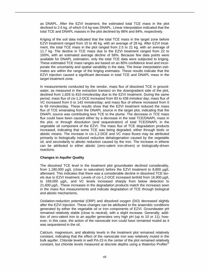
as DNAPL. After the EZVI treatment, the estimated total TCE mass in the plot declined to 2.6 kg, of which 0.6 kg was DNAPL. Linear interpolation indicated that the total TCE and DNAPL masses in the plot declined by 86% and 84%, respectively.

Kriging of the soil data indicated that the total TCE mass in the target zone before EZVI treatment ranged from 10 to 46 kg, with an average of 28 kg. After EZVI treat­ment, the total TCE mass in the plot ranged from 2.5 to 21 kg, with an average of 11.7 kg. The decline in TCE mass due to the EZVI treatment ranged from 22 to 100%, with an estimated average decline of 58%. Because few data points were available for DNAPL estimation, only the total TCE data were subjected to kriging. These estimated TCE mass ranges are based on an 80% confidence level and incor­porate the uncertainty and spatial variability in the data. The linear interpolation esti­mates are within the range of the kriging estimates. These results indicate that the EZVI injection caused a significant decrease in total TCE and DNAPL mass in the target treatment zone.

In measurements conducted by the vendor, mass flux of dissolved TCE in ground­water, as measured in the extraction transect on the downgradient side of the plot, declined from 1,826 to 810 mmoles/day due to the EZVI treatment. During the same period, mass flux of cis-1,2-DCE increased from 83 to 438 mmoles/ day; mass flux of VC increased from 0 to 143 mmoles/day; and mass flux of ethene increased from 0 to 69 mmoles/day. These results show that the EZVI treatment reduced the mass flux of TCE emanating from the DNAPL source in the target plot, indicating that the DNAPL source was contributing less TCE to the plume. The decrease in TCE mass flux could have been caused either by a decrease in the total TCE/DNAPL mass in the plot, or through dissolution (and sequestration) of total TCE/DNAPL in the vegetable oil component of the EZVI. The mass flux of TCE degradation products increased, indicating that some TCE was being degraded, either through biotic or abiotic means. The increase in cis-1,2-DCE and VC mass fluxes may be attributed primarily to biologically induced reductive dehalogenation caused by the vegetable oil, and secondarily to abiotic reduction caused by the iron. The increase in ethene can be attributed to either abiotic (zero-valent iron-driven) or biologically-driven reactions.

Changes in Aquifer Quality

The dissolved TCE level in the treatment plot groundwater declined considerably, from 1,180,000 µg/L (close to saturation) before the EZVI treatment to 8,800 µg/L afterward. This indicates that there was a considerable decline in dissolved TCE lev­els due to EZVI treatment. Levels of cis-1,2-DCE increased tenfold from 16,900 µg/L to 169,000 µg/L, and VC levels increased sharply from below detection to 21,600 µg/L. These increases in the degradation products match the increases seen in the mass flux measurements and indicate degradation of TCE through biological and abiotic mechanisms.

Oxidation-reduction potential (ORP) and dissolved oxygen (DO) decreased slightly after the EZVI injection. These changes can be attributed to the anaerobic conditions generated by either the vegetable oil or iron components of EZVI. Groundwater pH remained relatively stable (close to neutral), with a slight increase. Generally, addi­tion of zero-valent iron to an aquifer generates very high pH (up to 10 or 11); how­ever, in this case, the action of the nanoscale iron could have remained muted as it was sequestered in the oil.

Calcium, magnesium, and alkalinity levels in the treatment plot remained relatively constant, indicating that the effect of the nanoscale iron was relatively muted in the bulk aquifer. Chloride levels in well PA-23 in the center of the plot remained relatively constant, but chloride levels measured at discrete depths using a Waterloo Profiler®

vii

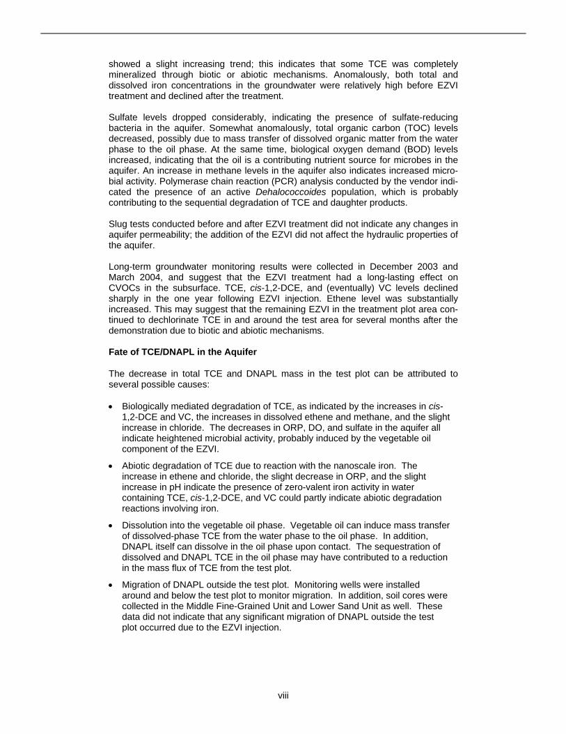
showed a slight increasing trend; this indicates that some TCE was completely mineralized through biotic or abiotic mechanisms. Anomalously, both total and dissolved iron concentrations in the groundwater were relatively high before EZVI treatment and declined after the treatment.

Sulfate levels dropped considerably, indicating the presence of sulfate-reducing bacteria in the aquifer. Somewhat anomalously, total organic carbon (TOC) levels decreased, possibly due to mass transfer of dissolved organic matter from the water phase to the oil phase. At the same time, biological oxygen demand (BOD) levels increased, indicating that the oil is a contributing nutrient source for microbes in the aquifer. An increase in methane levels in the aquifer also indicates increased micro­bial activity. Polymerase chain reaction (PCR) analysis conducted by the vendor indi­cated the presence of an active Dehalococcoides population, which is probably contributing to the sequential degradation of TCE and daughter products.

Slug tests conducted before and after EZVI treatment did not indicate any changes in aquifer permeability; the addition of the EZVI did not affect the hydraulic properties of the aquifer.

Long-term groundwater monitoring results were collected in December 2003 and March 2004, and suggest that the EZVI treatment had a long-lasting effect on CVOCs in the subsurface. TCE, cis-1,2-DCE, and (eventually) VC levels declined sharply in the one year following EZVI injection. Ethene level was substantially increased. This may suggest that the remaining EZVI in the treatment plot area con­tinued to dechlorinate TCE in and around the test area for several months after the demonstration due to biotic and abiotic mechanisms.

Fate of TCE/DNAPL in the Aquifer

The decrease in total TCE and DNAPL mass in the test plot can be attributed to several possible causes:

• Biologically mediated degradation of TCE, as indicated by the increases in cis ­1,2-DCE and VC, the increases in dissolved ethene and methane, and the slight increase in chloride. The decreases in ORP, DO, and sulfate in the aquifer all indicate heightened microbial activity, probably induced by the vegetable oil component of the EZVI.

• Abiotic degradation of TCE due to reaction with the nanoscale iron. The increase in ethene and chloride, the slight decrease in ORP, and the slight increase in pH indicate the presence of zero-valent iron activity in water containing TCE, cis-1,2-DCE, and VC could partly indicate abiotic degradation reactions involving iron.

• Dissolution into the vegetable oil phase. Vegetable oil can induce mass transfer of dissolved-phase TCE from the water phase to the oil phase. In addition, DNAPL itself can dissolve in the oil phase upon contact. The sequestration of dissolved and DNAPL TCE in the oil phase may have contributed to a reduction in the mass flux of TCE from the test plot.

• Migration of DNAPL outside the test plot. Monitoring wells were installed around and below the test plot to monitor migration. In addition, soil cores were collected in the Middle Fine-Grained Unit and Lower Sand Unit as well. These data did not indicate that any significant migration of DNAPL outside the test plot occurred due to the EZVI injection.

viii

Operating Requirements and Cost

As indicated by the changes in the aquifer chemistry, the EZVI injection was imple­mented with relative success, given the highly viscous nature of the emulsion. After initial evaluation of different delivery methods, PPT was used to inject the EZVI into the aquifer. The entire operation was relatively smooth and successful. Additional testing of the delivery method may be needed in the future to improve the distribution of the EZVI in the aquifer. The need to use the water recirculation system to help distribute the EZVI should be re-examined, as a significant amount of water was required to be treated aboveground before it could be reinjected.

A cost comparison between short-term source treatment with EZVI and long-term source/plume containment with an equivalent pump-and-treat system indicates that the EZVI treatment is cost-competitive.

ix

x

(Intentionally left blank)

Contents

Executive Summary...................................................................................................... vAppendices .................................................................................................................xivFigures........................................................................................................................ xvTables ........................................................................................................................xviiAcronyms and Abbreviations......................................................................................xix

1. Introduction ..............................................................................................................11.1 Project Background .........................................................................................1

1.1.1 Project Organization.............................................................................11.1.2 Performance Assessment ....................................................................11.1.3 The SITE Program ...............................................................................1

1.2 The DNAPL Problem .......................................................................................21.3 The Demonstration Site...................................................................................31.4 The EZVI Technology......................................................................................41.5 Technology Evaluation Report Structure.........................................................4

2. Site Characterization ...............................................................................................92.1 Hydrogeology of the Site .................................................................................9

2.1.1 The Surficial Aquifer at Launch Complex 34........................................92.1.2 The Semi-Confined Aquifer at Launch Complex 34...........................13

2.2 Surface Water Bodies at the Site ..................................................................162.3 DNAPL Contamination in the EZVI Plot and Vicinity.....................................162.4 Aquifer Quality at the Site..............................................................................20

3. Technology Operation ...........................................................................................213.1 EZVI Description............................................................................................213.2 Regulatory Requirements..............................................................................213.3 Application of EZVI Technology ....................................................................21

3.3.1 EZVI Injection Methods ......................................................................213.3.1.1 Direct Injection.....................................................................233.3.1.2 Liquid Atomization Injection.................................................233.3.1.3 Pressure Pulse Technology.................................................24

3.3.2 EZVI Injection Field Operations .........................................................253.4 Groundwater Control System ........................................................................283.5 Waste Handling and Disposal .......................................................................29

4. Performance Assessment Methodology................................................................314.1 Estimating Changes in TCE-DNAPL Mass and TCE Flux ............................31

4.1.1 Changes in TCE-DNAPL Mass ..........................................................314.1.2 Linear Interpolation by Contouring.....................................................364.1.3 Kriging ................................................................................................364.1.4 Interpreting the Results of the Two Mass Removal

Estimation Methods............................................................................37

xi

4.1.5 TCE Flux Measurements in Groundwater..........................................374.2 Evaluating Changes in Aquifer Quality ..........................................................374.3 Evaluating the Fate of the TCE-DNAPL ........................................................374.4 Verifying Operating Requirements and Costs ...............................................38

5. Performance Assessment Results and Conclusions.............................................395.1 Changes in TCE-DNAPL Mass in the Plot ....................................................39

5.1.1 Qualitative Evaluation of Changes in TCE-DNAPL Distribution ........395.1.2 TCE-DNAPL Mass Estimation by Linear Interpolation.......................445.1.3 TCE Mass Estimation by Kriging........................................................445.1.4 Groundwater Mass Flux .....................................................................455.1.5 Summary of Changes in the TCE-DNAPL Mass and Mass Flux

in the Plot ...........................................................................................465.2 Evaluating Changes in Aquifer Quality ..........................................................46

5.2.1 Changes in CVOC Levels in Groundwater ........................................475.2.2 Changes in Aquifer Geochemistry .....................................................495.2.3 Changes in Hydraulic Properties of the Aquifer .................................555.2.4 Changes in Biology of the EZVI Plot ..................................................555.2.5 Summary of Changes in Aquifer Quality............................................56

5.3 Evaluating the Fate of the TCE-DNAPL Mass ..............................................565.3.1 Abiotic Reductive Dechlorination of TCE ...........................................565.3.2 Microbial Reductive Dechlorination of TCE .......................................575.3.3 Potential for TCE-DNAPL Migration from the EZVI Plot ....................585.3.4 Summary Evaluation of the Fate of TCE-DNAPL ..............................64

5.4 Verifying Operating Requirements ................................................................64

6. Quality Assurance..................................................................................................676.1 QA Measures.................................................................................................67

6.1.1 Representativeness............................................................................676.1.2 Completeness ....................................................................................686.1.3 Chain of Custody................................................................................68

6.2 Field QC Measures........................................................................................686.2.1 Field QC for Soil Sampling.................................................................686.2.2 Field QC for Groundwater Sampling..................................................69

6.3 Laboratory QC Measures ..............................................................................706.3.1 Analytical QC for Soil Sampling .........................................................706.3.2 Laboratory QC for Groundwater Sampling ........................................706.3.3 Analytical Detection Limits .................................................................71

6.4 QA/QC Summary...........................................................................................71

7. Economic Analysis.................................................................................................737.1 EZVI Application Treatment Costs ................................................................737.2 Site Preparation and Waste Disposal Costs .................................................737.3 Site Characterization and Performance Assessment Costs..........................747.4 Present Value Analysis of EZVI Technology and Pump-and-Treat

System Costs.................................................................................................75

8. Technology Applications Analysis .........................................................................778.1 Objectives ......................................................................................................77

8.1.1 Overall Protection of Human Health and the Environment ................778.1.2 Compliance with ARARs ....................................................................77

8.1.2.1 Comprehensive Environmental Response, Compensation, and Liability Act ..........................................78

8.1.2.2 Resource Conservation and Recovery Act .........................788.1.2.3 Clean Water Act ..................................................................788.1.2.4 Safe Drinking Water Act ......................................................78

xii

8.1.2.5 Clean Air Act........................................................................798.1.2.6 Occupational Safety and Health Administration..................79

8.1.3 Long-Term Effectiveness ...................................................................798.1.4 Reduction of Toxicity, Mobility, or Volume through Treatment ..........808.1.5 Short-Term Effectiveness...................................................................808.1.6 Implementability .................................................................................808.1.7 Cost ....................................................................................................808.1.8 State (Support Agency) Acceptance..................................................818.1.9 Community Acceptance .....................................................................81

8.2 Operability......................................................................................................818.3 Applicable Wastes .........................................................................................818.4 Key Features .................................................................................................818.5 Availability/Transportability ............................................................................818.6 Materials Handling Requirements .................................................................828.7 Ranges of Suitable Site Characteristics ........................................................828.8 Limitations......................................................................................................82

9. References ............................................................................................................83

xiii

Appendices

Appendix A. Performance Assessment Methods A.1 Summary of Statistics A.2 Sample Collection and Extraction Methods A.3 List of Standard Sample Collection and Analytical Methods

Appendix B. Hydrogeologic Measurements B.1 Performance Monitoring Slug Tests B.2 Well Completion Diagrams B.3 Soil Coring Logsheets

Appendix C. CVOC Measurements Table C-1. CVOC Results of Groundwater Samples Table C-2. Summary of CVOC Results in Soil from EZVI Pre-

Demonstration Monitoring Table C-3. Summary of CVOC Results in Soil from EZVI Intermediate

Monitoring Table C-4. Summary of CVOC Results in Soil from EZVI Post-

Demonstration Monitoring Table C-5. Long-Term Groundwater Sampling

Appendix D. Inorganic and Other Aquifer Parameters Table D-1. Groundwater Field Parameters Table D-2. Inorganic Results of Groundwater from the EZVI Demonstration Table D-3. Other Parameter Results of Groundwater from the EZVI

Demonstration Table D-4. Results of Chloride Using Waterloo Profiler®

Table D-5. Results of Dissolved Gases in Groundwater from the EZVI Demonstration

Table D-6. Result of TOC in Soil Samples Prior to the EZVI Demonstration Table D-7. Mass Flux Measurements of Groundwater from the EZVI

Demonstration Table D-8. Genetrac Analysis of Groundwater Samples from the EZVI

Demonstration

Appendix E. Quality Assurance/Quality Control Information Tables E-1 to E-15

Appendix F. Economic Analysis Information Table F-1. Pump-and-Treat (P&T) System Design Basis Table F-2. Capital Investment for a P&T System Table F-3. Present Value of P&T System Costs for 30 Years of Operation Table F-4. Present Value of P&T System Costs for 100 Years of Operation Figure F-1. P&T System Costs for 100 Years

xiv

Figures

Figure 1-1. Project Organization for the EZVI Demonstration at Launch Complex 34 .............................................................................................2

Figure 1-2. Simplified Depiction of the Formation of a DNAPL Source Zone in the Subsurface ........................................................................................2

Figure 1-3. Location Map of Launch Complex 34 Site...............................................3Figure 1-4. Demonstration Site Location ...................................................................5Figure 1-5. View Looking South toward Launch Complex 34, the Engineering

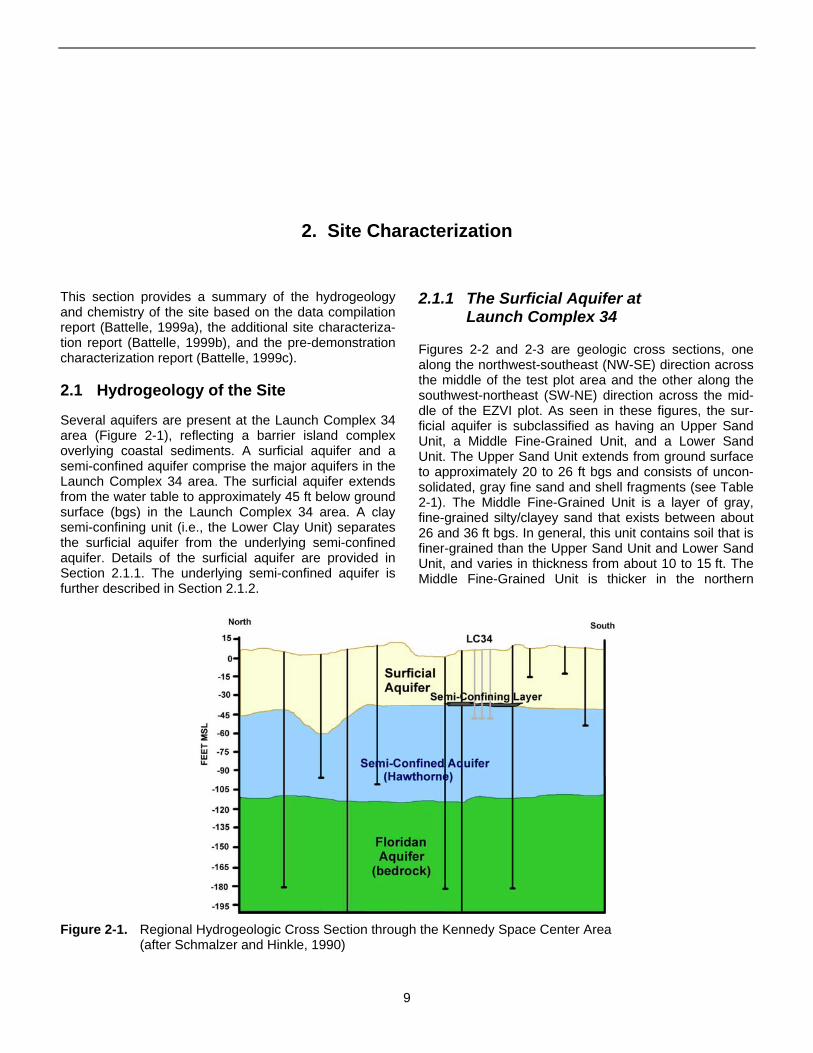
Support Building and Relative Location of EZVI Plot ..............................6Figure 1-6. Schematic of a Micelle Structure of the Emulsified Zero-Valent Iron......6Figure 1-7. Picture of Iron Particles Trapped Inside a Drop of Water-Oil Emulsion ..7Figure 1-8. Degradation Pathways for TCE with Zero-Valent Iron ............................7Figure 2-1. Regional Hydrogeologic Cross Section through the Kennedy Space

Center Area .............................................................................................9Figure 2-2. NW-SE Geologic Cross Section through the EZVI Plot ........................10Figure 2-3. SW-NE Geologic Cross Section through the EZVI Plot ........................10Figure 2-4. Water Table Elevation Map for Surficial Aquifer from June 1998 .........12Figure 2-5. Pre-Demonstration Water Levels (as elevation msl) in Shallow Wells

at Launch Complex 34 (March 2002) ....................................................13Figure 2-6. Pre-Demonstration Water Levels (as elevation msl) in Intermediate

Wells at Launch Complex 34 (March 2002) ..........................................14Figure 2-7. Pre-Demonstration Water Levels (as elevation msl) in Deep Wells

at Launch Complex 34 (March 2002) ....................................................14Figure 2-8. Pre-Demonstration Dissolved TCE Concentrations (µg/L) in Shallow

Wells in the EZVI Plot (March 2002) .....................................................17Figure 2-9. Pre-Demonstration Dissolved DCE Concentrations (µg/L) in Shallow

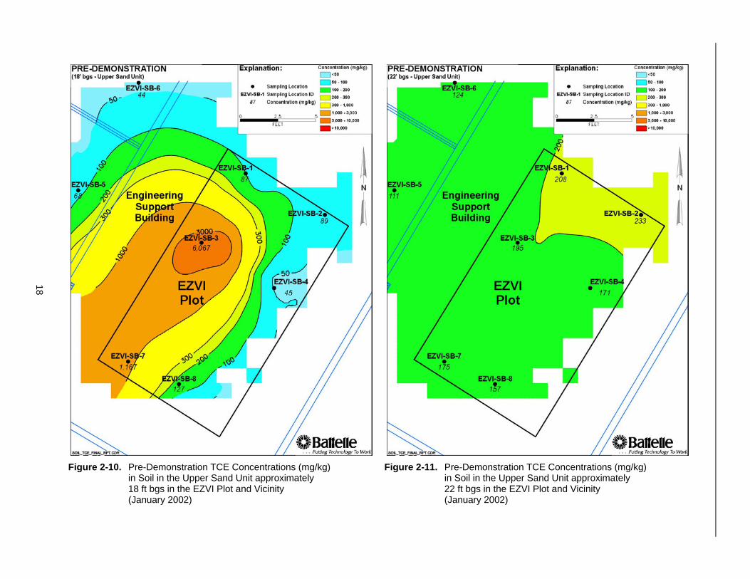
Wells in the EZVI Plot (March 2002) .....................................................17Figure 2-10. Pre-Demonstration TCE Concentrations (mg/kg) in Soil in the Upper

Sand Unit approximately 18 ft bgs in the EZVI Plot and Vicinity (January 2002) ......................................................................................18

Figure 2-11. Pre-Demonstration TCE Concentrations (mg/kg) in Soil in the Upper Sand Unit approximately 22 ft bgs in the EZVI Plot and Vicinity (January 2002) ......................................................................................18

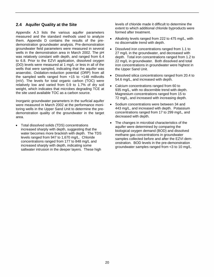
Figure 2-12. Vertical Cross Section through the EZVI Plot Showing Pre-Demonstration TCE Soil Concentrations (mg/kg) in the Subsurface ....19

Figure 2-13. Pre-Demonstration TCE Concentrations (mg/kg) as DNAPL in Soil in the Upper Sand Unit at Launch Complex 34 (January/February 2002) .......................................................................19

Figure 3-1. EZVI Experiments Using Pressure Pulse Technology, before (above) and after (below) ...........................................................24

Figure 3-2. Field Injection Test Setup with PPT Injection Technique ......................25Figure 3-3. Location Map and Injection Volume for EZVI Injection .........................26Figure 3-4. Aboveground Water Treatment System (A Series of Two Carbon

Tanks and a Backup Tank) ...................................................................29

xv

Figure 4-1. Soil Sampling for Performance Assessment at Launch Complex 34....31Figure 4-2. Soil Sample Collection (tan color indicates the native soil color; the

Figure 4-3. Pre-Demonstration Soil Boring Locations (SB-1 through SB-4; SB-7; gray to blackish band indicates evidence of the injected EZVI)..............32

SB-8) in the EZVI Plot (January/February 2002) ..................................33Figure 4-4. Post-Demonstration Soil Boring Locations (SB-201 through SB-204;

SB-207; SB-208; and SB-301 to SB-304; SB-307; SB-308) in the EZVI Plot (October 2002; November 2002) ..........................................34

Figure 4-5. Indoor Vibra-Push™ Rig (LD Geoprobe® Series) Used in the EZVI Plot Inside the Engineering Support Building...............................35

Figure 4-6. Collecting and Processing Groundwater Samples Using the Waterloo Profiler® ..................................................................................38

Figure 5-1. Distribution of TCE Concentrations (mg/kg) During Pre-Demonstration and Post-Demonstration Characterization in the EZVI Plot Soil ........................................................................................40

Figure 5-2. Representative (a) Pre-Demonstration (January 2002) and (b) Post-Demonstration (October to November 2002) Horizontal Cross Sec­tions of TCE (mg/kg) in soil at 18 ft bgs in the Upper Sand Unit Soil.... 41

Figure 5-3. Representative (a) Pre-Demonstration (January 2002) and (b) Post-Demonstration (October to November 2002) Horizontal Cross Sections of TCE (mg/kg) in soil at 22 ft bgs in the Upper Sand Unit .... 42

Figure 5-4. 3D Distribution of DNAPL in the EZVI Plot Based on (a) Pre-Demonstration (January 2002) and (b) Post-Demonstration (October to November 2002) Characterization .....................................43

Figure 5-5. Dissolved TCE Concentrations (µg/L) during (a) Pre-Demonstration (March 2002) and (b) Post-Demonstration (November 2002) Sampling of Shallow Wells ....................................................................50

Figure 5-6. Dissolved cis-1,2-DCE Concentrations (µg/L) during (a) Pre-Demonstration (March 2002) and (b) Post-Demonstration (November 2002) Sampling of Shallow Wells .......................................51

Figure 5-7. Dissolved Vinyl Chloride Concentrations (µg/L) during(a) Pre-Demonstration (March 2002) and (b) Post-Demonstration (November 2002) Sampling of Shallow Wells .......................................52

Figure 5-8. Chloride Increases Produced by the EZVI Treatment in

Figure 5-9a. Degradation Curve of TCE and Other CVOCs in PA-23 After

Figure 5-9b. Degradation Curve of TCE and Ethene in PA-23 After EZVI

Figure 5-10a.Water Levels Measured in Shallow Wells in the Engineering Support

Figure 5-10b.Water Levels Measured in Shallow Wells in the Engineering Support

Shallow Wells in and Around the Demonstration Plot...........................54

EZVI Treatment .....................................................................................60

Treatment ..............................................................................................60

Building During Pre-Demonstration Characterization (March 2002).....61

Building During the EZVI Technology Demonstration (August 2002) ...61Figure 5-10c. Water Levels Measured in Shallow Wells in the Engineering Support

Building During Post-Demonstration Characterization(November 2002)...................................................................................62

Figure 5-11a.Water Levels Measured in Intermediate Wells in the Engineering Support Building During Pre-Demonstration Characterization (March 2002) .........................................................................................62

Figure 5-11b.Water Levels Measured in Intermediate Wells in the Engineering Support Building During the EZVI Technology Demonstration (August 2002) ........................................................................................63

Figure 5-11c. Water Levels Measured in Intermediate Wells in the Engineering Support Building During Post-Demonstration Characterization(November 2002)...................................................................................63

Figure 5-12a.Pre-Demonstration TCE Concentrations (mg/kg) in Soil with Depth ....65Figure 5-12b.Post-Demonstration TCE Concentrations (mg/kg) in Soil with Depth...65

xvi

Tables

Table 2-1. Local Hydrostratigraphy at the Launch Complex 34 Site .........................11Table 2-2. Hydraulic Gradients and Directions in the Surficial and Semi-Confined

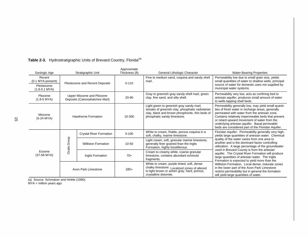
Aquifers.....................................................................................................13Table 2-3. Hydrostratigraphic Units of Brevard Country, Florida(a) ............................15Table 3-1. EZVI Demonstration Chronology..............................................................22Table 3-2. EZVI Demonstration Schedule .................................................................27Table 4-1. Summary of Performance Assessment Objectives and Associated

Measurements ..........................................................................................32Table 5-1. Estimated Total TCE and TCE-DNAPL Mass Reduction by Linear

Interpolation ..............................................................................................44Table 5-2. Estimated Total TCE Mass Reduction by Kriging.....................................45Table 5-3. Total Mass Discharge of CVOCs in Groundwater Before and After the

Demonstration ..........................................................................................46Table 5-4. CVOCs in Groundwater in the EZVI Plot Before and After

the Demonstration ....................................................................................47Table 5-5. Groundwater Parameters in the EZVI Plot Before and After the

Demonstration ..........................................................................................48Table 5-6. Dissolved Ethene and Ethane Concentrations in the EZVI Plot Before,

During, and After the Demonstration ........................................................58Table 5-7. Dissolved Methane Concentrations in the EZVI Plot Before, During,

and After the Demonstration.....................................................................58Table 5-8. TCE Degradation Byproducts in the EZVI Plot Before, During, and

After the Demonstration............................................................................59Table 6-1. Instruments and Calibration Acceptance Criteria Used for Field

Measurements ..........................................................................................68Table 6-2. List of Surrogate Compounds and Their Target Recoveries for Soil

and Groundwater Analysis by the Analytical Laboratory..........................70Table 7-1. EZVI Treatment Cost Summary Provided by Vendor...............................73Table 7-2. Estimated Site Characterization Costs .....................................................74Table 7-3. Estimated Performance Assessment Costs .............................................74

xvii

xviii

(Intentionally left blank)

Acronyms and Abbreviations

2D two-dimensional 3D three-dimensional

ACL alternative concentration limit ARAR applicable or relevant and appropriate requirement ARS ARS Technologies

bgs below ground surface BOD biological oxygen demand

CAA Clean Air Act CERCLA Comprehensive Environmental Response, Compensation,

and Liability Act CFR Code of Federal Regulations CVOC chlorinated volatile organic compound CWA Clean Water Act

DCE dichloroethylene DNAPL dense, nonaqueous-phase liquid DO dissolved oxygen

EEW EZVI extraction well EIW EZVI injection well EZVI emulsified zero-valent iron

FDEP (State of) Florida Department of Environmental Protection FRTR Federal Remediation Technology Roundtable

GAC granulated activated carbongpm gallon(s) per minute

HSWA Hazardous and Solid Waste Amendments

ISCO in situ chemical oxidation IW injection well

LAI liquid atomization injection LCS laboratory control spike(s) LRPCD Land Remediation and Pollution Control Division

MB method blank(s) MCL maximum contaminant level MS matrix spike(s) MSD matrix spike duplicate(s)

xix

msl mean sea level mV millivolts MYA million years ago

NA not available; not analyzed N/A not applicable NAAQS National Ambient Air Quality Standards NASA National Aeronautics and Space Administration ND not detected NPDES National Pollutant Discharge Elimination System

O&M operation and maintenance O.D. outside diameter ORD Office of Research and Development ORP oxidation-reduction potential OSHA Occupational Safety and Health Administration OW observation well

PCE tetrachloroethylene PCR polymerase chain reaction PLFA phospholipid fatty acid POTW publicly owned treatment works PPT pressure pulse technology psi pounds per square inch PV present value PVC polyvinyl chloride

QA quality assurance QAPP Quality Assurance Project Plan QC quality control

RCRA Resource Conservation and Recovery Act RFI RCRA Facility Investigation RI/FS Remedial Investigation/Feasibility Study RPD relative percent difference

SARA Superfund Amendments and Reauthorization Act SB soil boring SDWA Safe Drinking Water Act SI/E steam injection/extraction SIP State Implementation Plan SITE Superfund Innovative Technology Evaluation (Program) STTR Small Business Technology Transfer Research (Program)

TCA trichloroethane TCE trichloroethylene TDS total dissolved solids TOC total organic carbon

UCF University of Central Florida UIC Underground Injection Control U.S. EPA United States Environmental Protection Agency

VC vinyl chloride VOA volatile organic analysis

WP Waterloo Profiler®

xx

1. Introduction

This report presents the project field demonstration of emulsified zero-valent iron (EZVI) technology for treat­ment of a dense, nonaqueous-phase liquid (DNAPL) source zone at Launch Complex 34, Cape Canaveral Air Force Station, FL.

1.1 Project Background

The goal of the project was to evaluate the technical and cost performance of the nanoscale EZVI technology when applied to a DNAPL source zone. The chlorinated volatile organic compound (CVOC) trichloroethylene (TCE) is present as a DNAPL source in the aquifer at Launch Complex 34. Smaller amounts of dissolved cis­1,2-dichloroethylene (cis-1,2-DCE) and vinyl chloride (VC) also are present in the groundwater as a result of the natural degradation of TCE.

The field application of EZVI technology began at Launch Complex 34 in June 2002 and ended in January 2003. Performance assessment activities were con­ducted before, during, and after the field application.

1.1.1 Project Organization

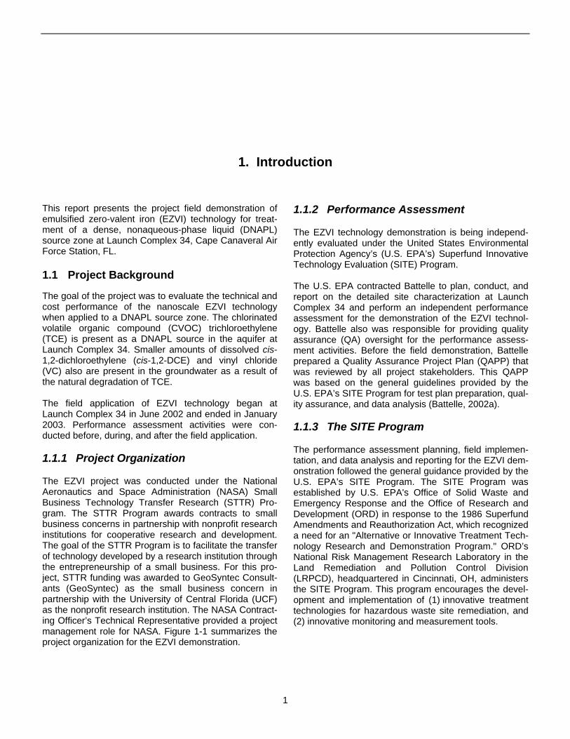
The EZVI project was conducted under the National Aeronautics and Space Administration (NASA) Small Business Technology Transfer Research (STTR) Pro­gram. The STTR Program awards contracts to small business concerns in partnership with nonprofit research institutions for cooperative research and development. The goal of the STTR Program is to facilitate the transfer of technology developed by a research institution through the entrepreneurship of a small business. For this pro­ject, STTR funding was awarded to GeoSyntec Consult­ants (GeoSyntec) as the small business concern in partnership with the University of Central Florida (UCF) as the nonprofit research institution. The NASA Contract­ing Officer’s Technical Representative provided a project management role for NASA. Figure 1-1 summarizes the project organization for the EZVI demonstration.

1.1.2 Performance Assessment

The EZVI technology demonstration is being independ­ently evaluated under the United States Environmental Protection Agency’s (U.S. EPA’s) Superfund Innovative Technology Evaluation (SITE) Program.

The U.S. EPA contracted Battelle to plan, conduct, and report on the detailed site characterization at Launch Complex 34 and perform an independent performance assessment for the demonstration of the EZVI technol­ogy. Battelle also was responsible for providing quality assurance (QA) oversight for the performance assess­ment activities. Before the field demonstration, Battelle prepared a Quality Assurance Project Plan (QAPP) that was reviewed by all project stakeholders. This QAPP was based on the general guidelines provided by the U.S. EPA’s SITE Program for test plan preparation, qual­ity assurance, and data analysis (Battelle, 2002a).

1.1.3 The SITE Program

The performance assessment planning, field implemen­tation, and data analysis and reporting for the EZVI dem­onstration followed the general guidance provided by the U.S. EPA’s SITE Program. The SITE Program was established by U.S. EPA's Office of Solid Waste and Emergency Response and the Office of Research and Development (ORD) in response to the 1986 Superfund Amendments and Reauthorization Act, which recognized a need for an "Alternative or Innovative Treatment Tech­nology Research and Demonstration Program." ORD’s National Risk Management Research Laboratory in the Land Remediation and Pollution Control Division (LRPCD), headquartered in Cincinnati, OH, administers the SITE Program. This program encourages the devel­opment and implementation of (1) innovative treatment technologies for hazardous waste site remediation, and (2) innovative monitoring and measurement tools.

1

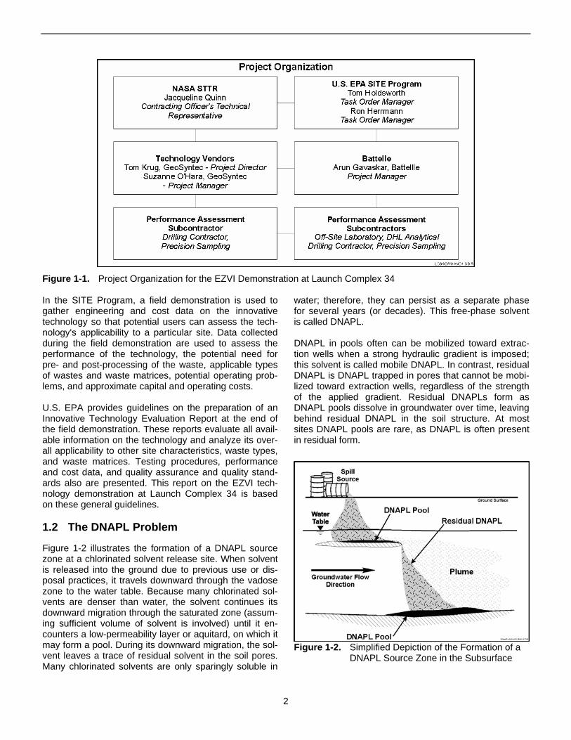
Figure 1-1. Project Organization for the EZVI Demonstration at Launch Complex 34

In the SITE Program, a field demonstration is used to gather engineering and cost data on the innovative technology so that potential users can assess the tech­nology's applicability to a particular site. Data collected during the field demonstration are used to assess the performance of the technology, the potential need for pre- and post-processing of the waste, applicable types of wastes and waste matrices, potential operating prob­lems, and approximate capital and operating costs.

U.S. EPA provides guidelines on the preparation of an Innovative Technology Evaluation Report at the end of the field demonstration. These reports evaluate all avail­able information on the technology and analyze its over­all applicability to other site characteristics, waste types, and waste matrices. Testing procedures, performance and cost data, and quality assurance and quality stand­ards also are presented. This report on the EZVI tech­nology demonstration at Launch Complex 34 is based on these general guidelines.

1.2 The DNAPL Problem

Figure 1-2 illustrates the formation of a DNAPL source zone at a chlorinated solvent release site. When solvent is released into the ground due to previous use or dis­posal practices, it travels downward through the vadose zone to the water table. Because many chlorinated sol­vents are denser than water, the solvent continues its downward migration through the saturated zone (assum­ing sufficient volume of solvent is involved) until it en­counters a low-permeability layer or aquitard, on which it may form a pool. During its downward migration, the sol­vent leaves a trace of residual solvent in the soil pores. Many chlorinated solvents are only sparingly soluble in

water; therefore, they can persist as a separate phase for several years (or decades). This free-phase solvent is called DNAPL.

DNAPL in pools often can be mobilized toward extrac­tion wells when a strong hydraulic gradient is imposed; this solvent is called mobile DNAPL. In contrast, residual DNAPL is DNAPL trapped in pores that cannot be mobi­lized toward extraction wells, regardless of the strength of the applied gradient. Residual DNAPLs form as DNAPL pools dissolve in groundwater over time, leaving behind residual DNAPL in the soil structure. At most sites DNAPL pools are rare, as DNAPL is often present in residual form.

Figure 1-2. Simplified Depiction of the Formation of a DNAPL Source Zone in the Subsurface

2

As long as DNAPL is present in the aquifer, a plume of dissolved solvent is generated. DNAPL therefore consti­tutes a secondary source that keeps replenishing the plume long after the primary source (leaking above-ground or buried drums, drain pipes, vadose zone soil, etc.) has been removed. Because DNAPL persists for many decades or centuries, the resulting plume also per­sists for many years. As recently as five years ago, DNAPL sources were difficult to find and most remedial approaches focused on plume treatment or plume con­trol. In recent years, efforts to identify DNAPL sources have been successful at many chlorinated solvent-contaminated sites. The focus is now shifting from plume control to DNAPL source removal or treatment.

Pump-and-treat systems have been the conventional treatment approach at DNAPL sites and these systems have proven useful as an interim remedy to control the progress of the plume beyond a property boundary or other compliance point. However, pump-and-treat

systems are not economical for DNAPL remediation. Pools of DNAPL that can be pumped and treated above ground are rare. Residual DNAPL is immobile and does not migrate toward extraction wells. As with plume con­trol, the effectiveness and cost of DNAPL remediation with pump and treat is governed by the time (decades) required for slow dissolution of the DNAPL source in the groundwater flow. An innovative approach is required to address the DNAPL problem.

1.3 The Demonstration Site

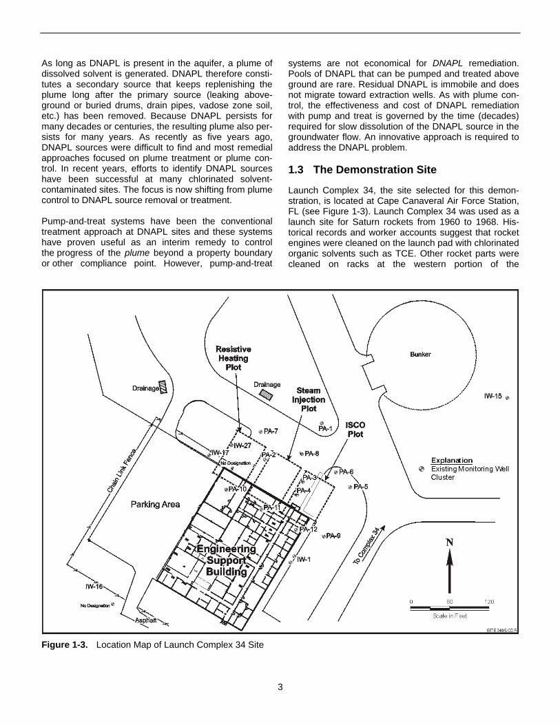
Launch Complex 34, the site selected for this demon­stration, is located at Cape Canaveral Air Force Station, FL (see Figure 1-3). Launch Complex 34 was used as a launch site for Saturn rockets from 1960 to 1968. His­torical records and worker accounts suggest that rocket engines were cleaned on the launch pad with chlorinated organic solvents such as TCE. Other rocket parts were cleaned on racks at the western portion of the

Figure 1-3. Location Map of Launch Complex 34 Site

3

Engineering Support Building and inside the building. Some of the solvents ran off to the surface or discharged into drainage pits. The site was abandoned in 1968; since then, much of the site has been overgrown by vegetation, although several on-site buildings remain operational.

Preliminary site characterization efforts suggested that approximately 20,600 kg (Battelle, 1999a) to 40,000 kg (Eddy-Dilek et al., 1998) of solvent could be present in the subsurface near the Engineering Support Building. Figure 1-4 is a map of the Launch Complex 34 site that shows the target DNAPL source area for the EZVI tech­nology demonstration, located inside the Engineering Support Building. Figure 1-5 is a photograph looking south toward the EZVI plot inside the Engineering Sup­port Building.

1.4 The EZVI Technology

EZVI can be used to enhance the dehalogenation of chlorinated DNAPL in source zones by creating intimate contact between the DNAPL and the nanoscale iron par­ticles. The EZVI is composed of surfactant, biodegrad­able oil, water, and nanoscale zero-valent iron particles, which form emulsion particles (or micelles) that contain the iron particles in water surrounded by an oil-liquid membrane. Figure 1-6 is a schematic drawing of an EZVI micelle, and Figure 1-7 is a photograph of iron particles visible inside an emulsion drop. Because the exterior oil membrane of an emulsion particle has similar hydrophobic properties as the DNAPL, the emulsion is miscible with the DNAPL (i.e., the phases can mix).

Laboratory experiments conducted at UCF for NASA have demonstrated that DNAPL compounds (e.g., TCE) diffuse through the oil membrane of the emulsion particle and undergo reductive dechlorination facilitated by the zero-valent iron particles in the interior aqueous phase. The final byproducts from the dehalogenation reaction (i.e., nonchlorinated hydrocarbons) then can diffuse out of the emulsion into the surrounding aqueous phase. The main dehalogenation reaction pathways occurring at the iron surface require excess electrons, which are pro­duced from the corrosion of the zero-valent iron in water as follows:

Fe0 → Fe2+ + 2e− (1)

Fe2+(surface) → Fe3+

(aqueous) + e− (2)

Hydrogen gas also is produced, as well as OH− , which results in an increase in the pH of the surrounding water according to the following reaction:

2H2O + 2 e− → H2(gas) + 2OH− (3)

Some portion of the chlorinated ethenes is degraded by a stepwise dehalogenation reaction according to:

RCl− + H+ + 2e− → RH + Cl− (4)

In the dehalogenation step, reaction (4), the “R” repre­sents the molecular group to which the chlorine atom is attached. In the case of TCE, R would be the CHClCl−

fragment. For the total dehalogenation of TCE, reaction (4) must occur three times, with the end product being ethene. The degradation of TCE also occurs via a β ­elimination reaction where TCE is converted to chloro­acetylene followed by a dehalogenation reaction to acetylene. The acetylene degrades to ethene and then to ethane. Figure 1-8 illustrates the degradation pathways for TCE using zero-valent iron. The predominant path­way for degradation of chlorinated ethenes is reported to be the β-elimination pathway (Roberts et al., 1996). Laboratory studies conducted at UCF have shown that complete dehalogenation occurs within the EZVI micelles (UCF, 2000).

Before the EZVI demonstration was started, concerns were raised about the potential difficulties associated with the injection and subsurface distribution of the emul­sion. Concerns also were raised about the effectiveness of the recirculation system designed to establish steady state flow conditions in the test plot, and the possibility of contaminant dilution or drawing in contaminated water from outside the plot boundaries. The installation and oper­ation of the EZVI technology is described in Section 3.

1.5 Technology Evaluation Report Structure

The EZVI technology evaluation report starts with an introduction to the project organization, the DNAPL prob­lem, the technology demonstrated, and the demonstra­tion site (Section 1). The rest of the report is organized as follows:

• Site Characterization (Section 2)

• Technology Operation (Section 3)

• Performance Assessment Methodology (Section 4)

• Performance Assessment Results and Conclusions (Section 5)

• Quality Assurance (Section 6)

• Economic Analysis (Section 7)

• Technology Applications Analysis (Section 8)

• References (Section 9).

4

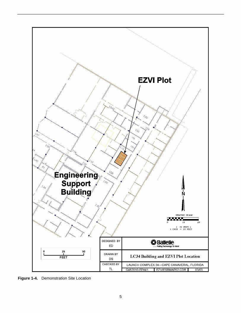
Figure 1-4. Demonstration Site Location

5

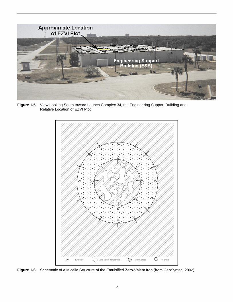
Figure 1-5. View Looking South toward Launch Complex 34, the Engineering Support Building and Relative Location of EZVI Plot

Figure 1-6. Schematic of a Micelle Structure of the Emulsified Zero-Valent Iron (from GeoSyntec, 2002)

6

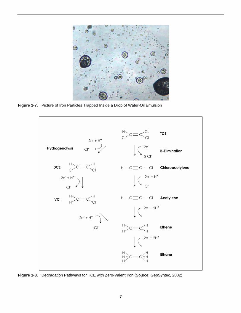
Figure 1-7. Picture of Iron Particles Trapped Inside a Drop of Water-Oil Emulsion

Figure 1-8. Degradation Pathways for TCE with Zero-Valent Iron (Source: GeoSyntec, 2002)

7

Supporting data and other information are presented in the appendices to the report. The appendices are orga­nized as follows:

• Performance Assessment Methods (Appendix A)

• Hydrogeologic Measurements (Appendix B)

• CVOC Measurements (Appendix C)

• Inorganic and Other Aquifer Parameters (Appendix D)

• Quality Assurance/Quality Control Information (Appendix E)

• Economic Analysis Information (Appendix F)

8

2. Site Characterization

This section provides a summary of the hydrogeology and chemistry of the site based on the data compilation report (Battelle, 1999a), the additional site characteriza­tion report (Battelle, 1999b), and the pre-demonstration characterization report (Battelle, 1999c).

2.1 Hydrogeology of the Site

Several aquifers are present at the Launch Complex 34 area (Figure 2-1), reflecting a barrier island complex overlying coastal sediments. A surficial aquifer and a semi-confined aquifer comprise the major aquifers in the Launch Complex 34 area. The surficial aquifer extends from the water table to approximately 45 ft below ground surface (bgs) in the Launch Complex 34 area. A clay semi-confining unit (i.e., the Lower Clay Unit) separates the surficial aquifer from the underlying semi-confined aquifer. Details of the surficial aquifer are provided in Section 2.1.1. The underlying semi-confined aquifer is further described in Section 2.1.2.

2.1.1 The Surficial Aquifer at Launch Complex 34

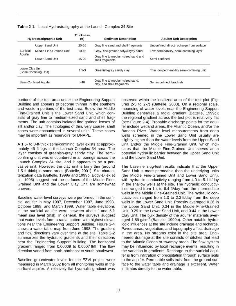
Figures 2-2 and 2-3 are geologic cross sections, one along the northwest-southeast (NW-SE) direction across the middle of the test plot area and the other along the southwest-northeast (SW-NE) direction across the mid­dle of the EZVI plot. As seen in these figures, the sur­ficial aquifer is subclassified as having an Upper Sand Unit, a Middle Fine-Grained Unit, and a Lower Sand Unit. The Upper Sand Unit extends from ground surface to approximately 20 to 26 ft bgs and consists of uncon­solidated, gray fine sand and shell fragments (see Table 2-1). The Middle Fine-Grained Unit is a layer of gray, fine-grained silty/clayey sand that exists between about 26 and 36 ft bgs. In general, this unit contains soil that is finer-grained than the Upper Sand Unit and Lower Sand Unit, and varies in thickness from about 10 to 15 ft. The Middle Fine-Grained Unit is thicker in the northern

Figure 2-1. Regional Hydrogeologic Cross Section through the Kennedy Space Center Area (after Schmalzer and Hinkle, 1990)

9

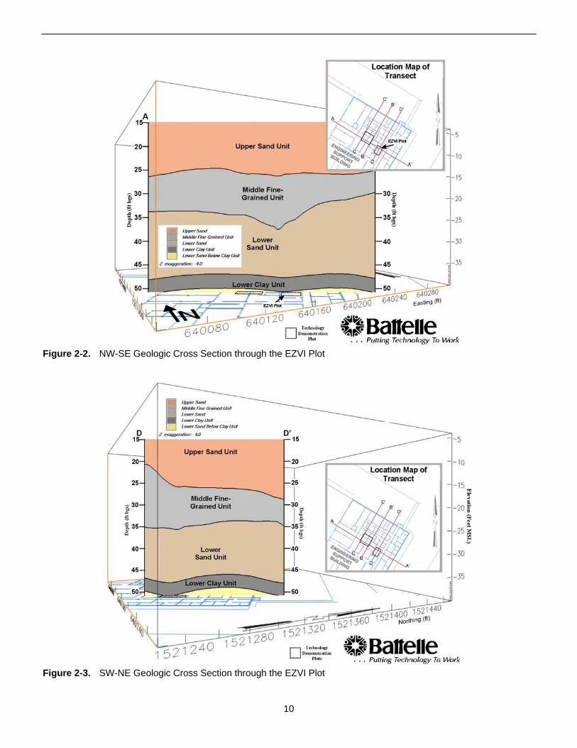
Figure 2-2. NW-SE Geologic Cross Section through the EZVI Plot

Figure 2-3. SW-NE Geologic Cross Section through the EZVI Plot

10

Hydrostratigraphic Unit Thickness

(ft) Sediment Description Aquifer Unit Description

Surficial Aquifer

Upper Sand Unit

Middle Fine-Grained Unit

Lower Sand Unit

20-26

10-15

15-20

Gray fine sand and shell fragments

Gray, fine-grained silty/clayey sand

Gray fine to medium-sized sand and shell fragments

Unconfined, direct recharge from surface

Low-permeability, semi-confining layer

Semi-confined

Lower Clay Unit (Semi-Confining Unit) 1.5-3 Greenish-gray sandy clay Thin low-permeability semi-confining unit

Semi-Confined Aquifer >40 Gray fine to medium-sized sand, clay, and shell fragments Semi-confined, brackish

Table 2-1. Local Hydrostratigraphy at the Launch Complex 34 Site

portions of the test area under the Engineering Support Building and appears to become thinner in the southern and western portions of the test area. Below the Middle Fine-Grained Unit is the Lower Sand Unit, which con­sists of gray fine to medium-sized sand and shell frag­ments. The unit contains isolated fine-grained lenses of silt and/or clay. The lithologies of thin, very coarse, shell zones were encountered in several units. These zones may be important as reservoirs for DNAPL.

A 1.5- to 3-ft-thick semi-confining layer exists at approxi­mately 45 ft bgs in the Launch Complex 34 area. The layer consists of greenish-gray sandy clay. The semi-confining unit was encountered in all borings across the Launch Complex 34 site, and it appears to be a per­vasive unit. However, the clay unit is fairly thin (around 1.5 ft thick) in some areas (Battelle, 2001). Site charac­terization data (Battelle, 1999a and 1999b; Eddy-Dilek et al., 1998) suggest that the surfaces of the Middle Fine-Grained Unit and the Lower Clay Unit are somewhat uneven.

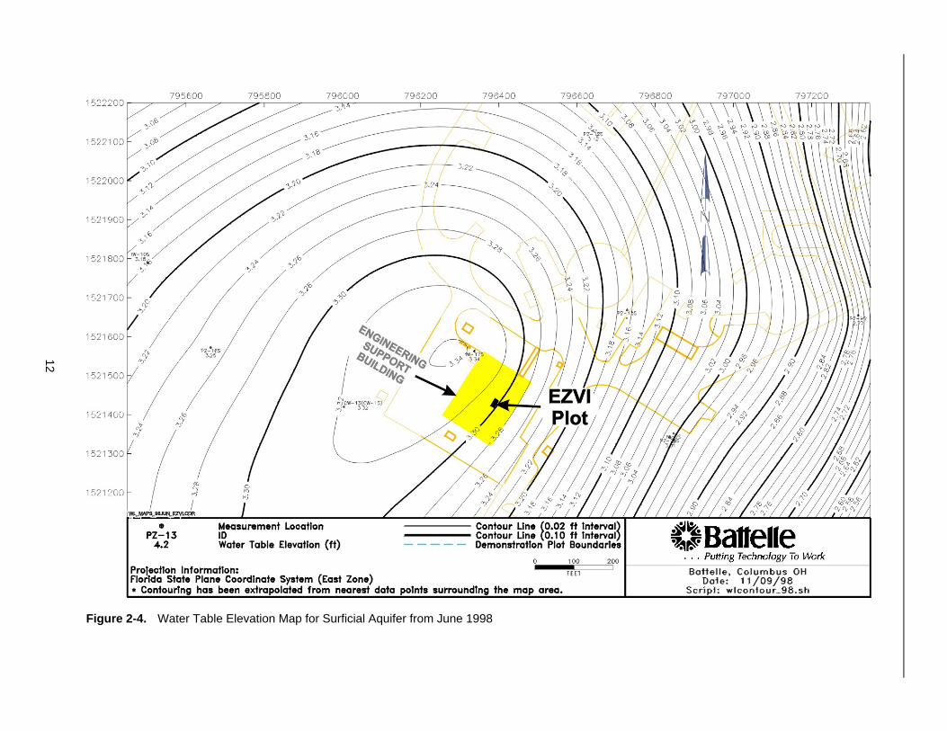
Baseline water level surveys were performed in the surfi­cial aquifer in May 1997, December 1997, June 1998, October 1998, and March 1999. Water table elevations in the surficial aquifer were between about 1 and 5 ft mean sea level (msl). In general, the surveys suggest that water levels form a radial pattern with highest eleva­tions near the Engineering Support Building. Figure 2-4 shows a water-table map from June 1998. The gradient and flow directions vary over time at the site. Table 2-2 summarizes the hydraulic gradients and their directions near the Engineering Support Building. The horizontal gradient ranged from 0.00009 to 0.0007 ft/ft. The flow direction varied from north-northeast to south-southwest.

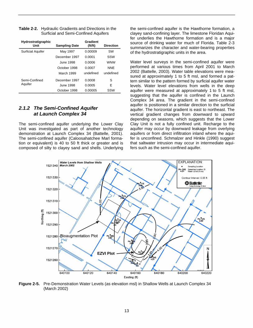
Baseline groundwater levels for the EZVI project were measured in March 2002 from all monitoring wells in the surficial aquifer. A relatively flat hydraulic gradient was

observed within the localized area of the test plot (Fig­ures 2-5 to 2-7) (Battelle, 2003). On a regional scale, mounding of water levels near the Engineering Support Building generates a radial gradient (Battelle, 1999c); the regional gradient across the test plot is relatively flat (see Figure 2-4). Probable discharge points for the aqui­fer include wetland areas, the Atlantic Ocean, and/or the Banana River. Water level measurements from deep wells screened in the Lower Sand Unit usually are slightly higher than the water levels from the Upper Sand Unit and/or the Middle Fine-Grained Unit, which indi­cates that the Middle Fine-Grained Unit serves as a potential hydraulic barrier between the Upper Sand Unit and the Lower Sand Unit.

The baseline slug-test results indicate that the Upper Sand Unit is more permeable than the underlying units (the Middle Fine-Grained Unit and Lower Sand Unit), with hydraulic conductivity ranging from 4.0 to 5.1 ft/day in the shallow wells at the site. The hydraulic conductiv­ities ranged from 1.4 to 6.4 ft/day from the intermediate wells in the Middle Fine-Grained Unit. The hydraulic con­ductivities ranged from 1.3 to 2.3 ft/day from the deep wells in the Lower Sand Unit. Porosity averaged 0.26 in the Upper Sand Unit, 0.34 in the Middle Fine-Grained Unit, 0.29 in the Lower Sand Unit, and 0.44 in the Lower Clay Unit. The bulk density of the aquifer materials aver­aged 1.59 g/cm3 (Battelle, 1999b). Other notable hydro­logic influences at the site include drainage and recharge. Paved areas, vegetation, and topography affect drainage in the area. No streams exist in the site area. Engi­neered drainage at the site consists of ditches that lead to the Atlantic Ocean or swampy areas. The flow system may be influenced by local recharge events, resulting in the variation in gradients. Recharge to the surficial aqui­fer is from infiltration of precipitation through surface soils to the aquifer. Permeable soils exist from the ground sur­face to the water table and drainage is excellent. Water infiltrates directly to the water table.

11

12

Figure 2-4. Water Table Elevation Map for Surficial Aquifer from June 1998

Hydrostratigraphic Unit Sampling Date

Gradient (ft/ft) Direction

Surficial Aquifer May 1997 0.00009 SW December 1997 0.0001 SSW June 1998 0.0006 WNW October 1998 0.0007 NNE

March 1999 undefined undefined

Semi-Confined December 1997 0.0008 S Aquifer June 1998 0.0005 E October 1998 0.00005 SSW

Table 2-2. Hydraulic Gradients and Directions in the Surficial and Semi-Confined Aquifers

2.1.2 The Semi-Confined Aquifer at Launch Complex 34

The semi-confined aquifer underlying the Lower Clay Unit was investigated as part of another technology demonstration at Launch Complex 34 (Battelle, 2001). The semi-confined aquifer (Caloosahatchee Marl forma­tion or equivalent) is 40 to 50 ft thick or greater and is composed of silty to clayey sand and shells. Underlying

the semi-confined aquifer is the Hawthorne formation, a clayey sand-confining layer. The limestone Floridan Aqui­fer underlies the Hawthorne formation and is a major source of drinking water for much of Florida. Table 2-3 summarizes the character and water-bearing properties of the hydrostratigraphic units in the area.

Water level surveys in the semi-confined aquifer were performed at various times from April 2001 to March 2002 (Battelle, 2003). Water table elevations were mea­sured at approximately 1 to 5 ft msl, and formed a pat­tern similar to the pattern formed by surficial aquifer water levels. Water level elevations from wells in the deep aquifer were measured at approximately 1 to 5 ft msl, suggesting that the aquifer is confined in the Launch Complex 34 area. The gradient in the semi-confined aquifer is positioned in a similar direction to the surficial aquifer. The horizontal gradient is east to northeast. The vertical gradient changes from downward to upward depending on seasons, which suggests that the Lower Clay Unit is not a fully confined unit. Recharge to the aquifer may occur by downward leakage from overlying aquifers or from direct infiltration inland where the aqui­fer is unconfined. Schmalzer and Hinkle (1990) suggest that saltwater intrusion may occur in intermediate aqui­fers such as the semi-confined aquifer.

Figure 2-5. Pre-Demonstration Water Levels (as elevation msl) in Shallow Wells at Launch Complex 34 (March 2002)

13

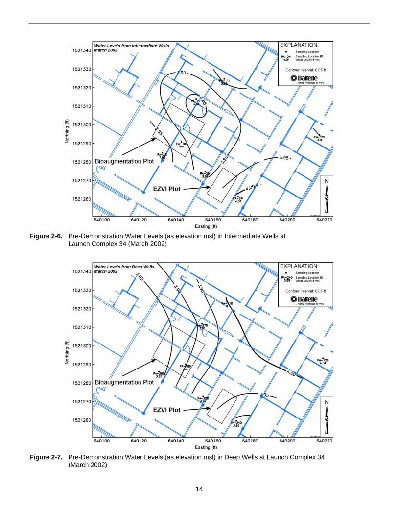
Figure 2-6. Pre-Demonstration Water Levels (as elevation msl) in Intermediate Wells at Launch Complex 34 (March 2002)

Figure 2-7. Pre-Demonstration Water Levels (as elevation msl) in Deep Wells at Launch Complex 34 (March 2002)

14

Oca

la G

roup

Approximate

Geologic Age Stratigraphic Unit Thickness (ft) General Lithologic Character Water-Bearing Properties Recent Fine to medium sand, coquina and sandy shell Permeability low due to small grain size, yields

(0.1 MYA-present) marl. small quantities of water to shallow wells, principal Pleistocene and Recent Deposits 0-110 source of water for domestic uses not supplied by Pleistocene

municipal water systems. (1.8-0.1 MYA) Gray to greenish gray sandy shell marl, green Permeability very low, acts as confining bed to Pliocene Upper Miocene and Pliocene 20-90 clay, fine sand, and silty shell. artesian aquifer, produces small amount of water (1.8-5 MYA) Deposits (Caloosahatchee Marl) to wells tapping shell beds. Light green to greenish gray sandy marl, Permeability generally low, may yield small quanti­streaks of greenish clay, phosphatic radiolarian ties of fresh water in recharge areas, generally clay, black and brown phosphorite, thin beds of permeated with water from the artesian zone. Miocene Hawthorne Formation 10-300 phosphatic sandy limestone. Contains relatively impermeable beds that prevent (5-24 MYA) or retard upward movement of water from the

underlying artesian aquifer. Basal permeable beds are considered part of the Floridan Aquifer.

White to cream, friable, porous coquina in a Floridan Aquifer: Permeability generally very high, Crystal River Formation 0-100 soft, chalky, marine limestone. yields large quantities of artesian water. Chemical quality of the water varies from one area to Light cream, soft, granular marine limestone, another and is the dominant factor controlling Williston Formation 10-50 generally finer grained than the Inglis utilization. A large percentage of the groundwater Formation, highly fossiliferous. used in Brevard County is from the artesian Eocene Cream to creamy white, coarse granular aquifer. The Crystal River Formation will produce (37-58 MYA) Inglis Formation 70+ limestone, contains abundant echinoid large quantities of artesian water. The Inglis

fragments. Formation is expected to yield more than the White to cream, purple tinted, soft, dense Williston Formation. Local dense, indurate zones chalky limestone. Localized zones of altered in the lower part of the Avon Park Limestone Avon Park Limestone 285+ to light brown or ashen gray, hard, porous, restrict permeability but in general the formation crystalline dolomite. will yield large quantities of water.

(a) Source: Schmalzer and Hinkle (1990). MYA = million years ago.

15

Table 2-3. Hydrostratigraphic Units of Brevard Country, Florida(a)

2.2 Surface Water Bodies at the Site

The major surface water body in the area is the Atlantic Ocean, located to the east of Launch Complex 34. To determine the effects of surface water bodies on the groundwater system, water levels were monitored in 12 piezometers for more than 50 hours for a tidal influ­ence study during Resource Conservation and Recovery Act (RCRA) Facility Investigation (RFI) activities (G&E Engineering, Inc., 1996). All the piezometers used in the study were screened in the surficial aquifer. No detect­able effects from the tidal cycles were measured, sug­gesting that the surficial aquifer and the Atlantic Ocean are not well connected hydraulically. However, the Atlantic Ocean and the Banana River seem to act as hydraulic barriers or sinks, as groundwater likely flows toward these surface water bodies and discharges into them.

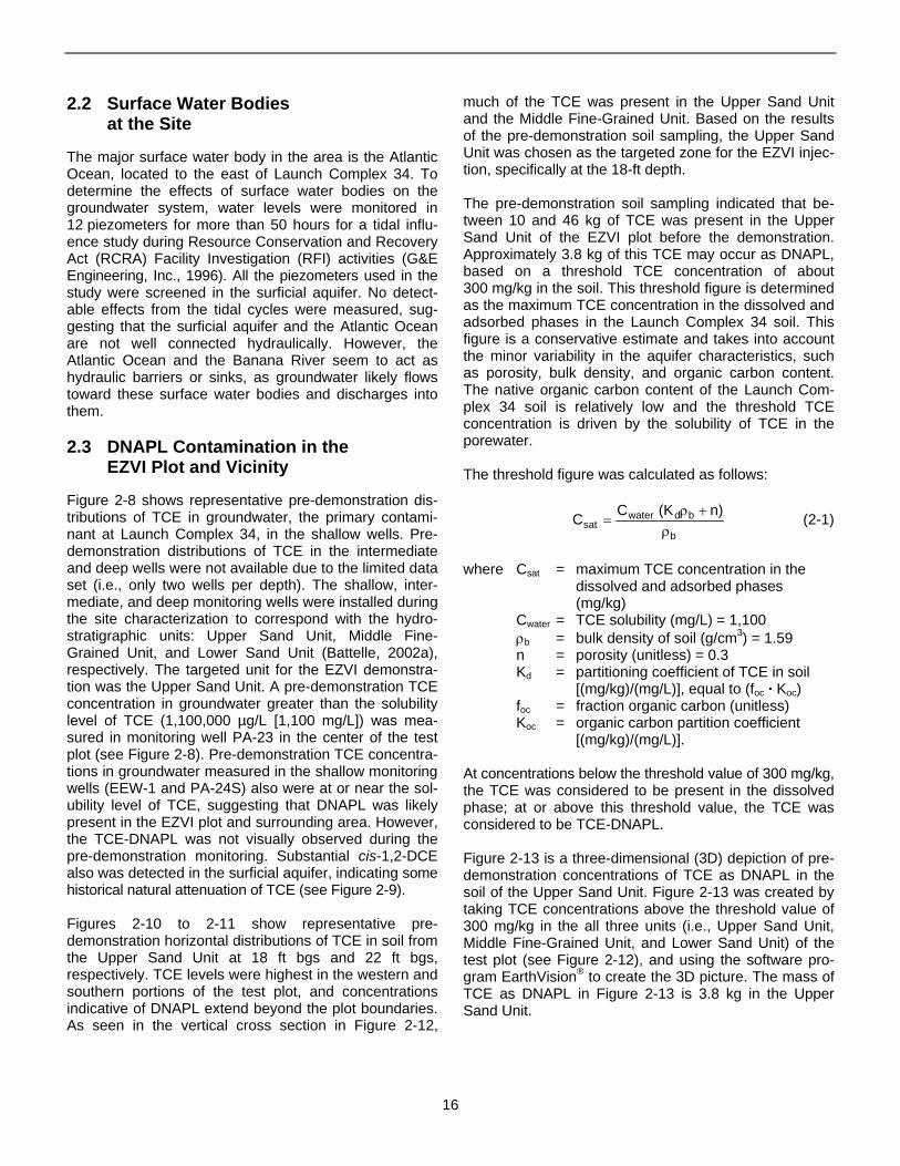
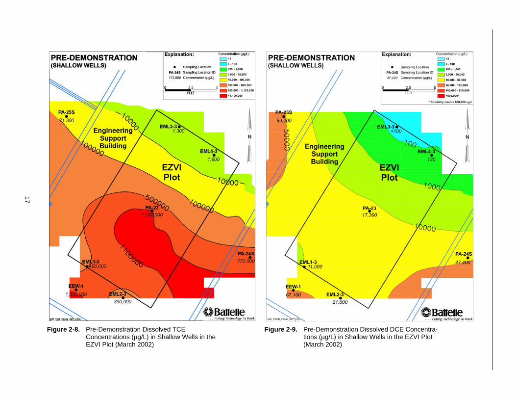
2.3 DNAPL Contamination in the EZVI Plot and Vicinity

Figure 2-8 shows representative pre-demonstration dis­tributions of TCE in groundwater, the primary contami­nant at Launch Complex 34, in the shallow wells. Pre-demonstration distributions of TCE in the intermediate and deep wells were not available due to the limited data set (i.e., only two wells per depth). The shallow, inter­mediate, and deep monitoring wells were installed during the site characterization to correspond with the hydro-stratigraphic units: Upper Sand Unit, Middle Fine-Grained Unit, and Lower Sand Unit (Battelle, 2002a), respectively. The targeted unit for the EZVI demonstra­tion was the Upper Sand Unit. A pre-demonstration TCE concentration in groundwater greater than the solubility level of TCE (1,100,000 µg/L [1,100 mg/L]) was mea­sured in monitoring well PA-23 in the center of the test plot (see Figure 2-8). Pre-demonstration TCE concentra­tions in groundwater measured in the shallow monitoring wells (EEW-1 and PA-24S) also were at or near the sol­ubility level of TCE, suggesting that DNAPL was likely present in the EZVI plot and surrounding area. However, the TCE-DNAPL was not visually observed during the pre-demonstration monitoring. Substantial cis-1,2-DCE also was detected in the surficial aquifer, indicating some historical natural attenuation of TCE (see Figure 2-9).

Figures 2-10 to 2-11 show representative pre-demonstration horizontal distributions of TCE in soil from the Upper Sand Unit at 18 ft bgs and 22 ft bgs, respectively. TCE levels were highest in the western and southern portions of the test plot, and concentrations indicative of DNAPL extend beyond the plot boundaries. As seen in the vertical cross section in Figure 2-12,

much of the TCE was present in the Upper Sand Unit and the Middle Fine-Grained Unit. Based on the results of the pre-demonstration soil sampling, the Upper Sand Unit was chosen as the targeted zone for the EZVI injec­tion, specifically at the 18-ft depth.

The pre-demonstration soil sampling indicated that be­tween 10 and 46 kg of TCE was present in the Upper Sand Unit of the EZVI plot before the demonstration. Approximately 3.8 kg of this TCE may occur as DNAPL, based on a threshold TCE concentration of about 300 mg/kg in the soil. This threshold figure is determined as the maximum TCE concentration in the dissolved and adsorbed phases in the Launch Complex 34 soil. This figure is a conservative estimate and takes into account the minor variability in the aquifer characteristics, such as porosity, bulk density, and organic carbon content. The native organic carbon content of the Launch Com­plex 34 soil is relatively low and the threshold TCE concentration is driven by the solubility of TCE in the porewater.

The threshold figure was calculated as follows:

C =Cwater (Kdρb + n) (2-1) sat ρb

where Csat = maximum TCE concentration in the dissolved and adsorbed phases (mg/kg)

Cwater = TCE solubility (mg/L) = 1,100 ρb = bulk density of soil (g/cm3) = 1.59 n = porosity (unitless) = 0.3 Kd = partitioning coefficient of TCE in soil

[(mg/kg)/(mg/L)], equal to (foc · Koc) foc = fraction organic carbon (unitless) Koc = organic carbon partition coefficient

[(mg/kg)/(mg/L)].

At concentrations below the threshold value of 300 mg/kg, the TCE was considered to be present in the dissolved phase; at or above this threshold value, the TCE was considered to be TCE-DNAPL.

Figure 2-13 is a three-dimensional (3D) depiction of pre-demonstration concentrations of TCE as DNAPL in the soil of the Upper Sand Unit. Figure 2-13 was created by taking TCE concentrations above the threshold value of 300 mg/kg in the all three units (i.e., Upper Sand Unit, Middle Fine-Grained Unit, and Lower Sand Unit) of the test plot (see Figure 2-12), and using the software pro­gram EarthVision® to create the 3D picture. The mass of TCE as DNAPL in Figure 2-13 is 3.8 kg in the Upper Sand Unit.

16

17

Figure 2-8. Pre-Demonstration Dissolved TCE Concentrations (µg/L) in Shallow Wells in the

Figure 2-9. Pre-Demonstration Dissolved DCE Concentra­tions (µg/L) in Shallow Wells in the EZVI Plot

EZVI Plot (March 2002) (March 2002)

18

Figure 2-10. Pre-Demonstration TCE Concentrations (mg/kg) Figure 2-11. Pre-Demonstration TCE Concentrations (mg/kg) in Soil in the Upper Sand Unit approximately in Soil in the Upper Sand Unit approximately 18 ft bgs in the EZVI Plot and Vicinity 22 ft bgs in the EZVI Plot and Vicinity (January 2002) (January 2002)

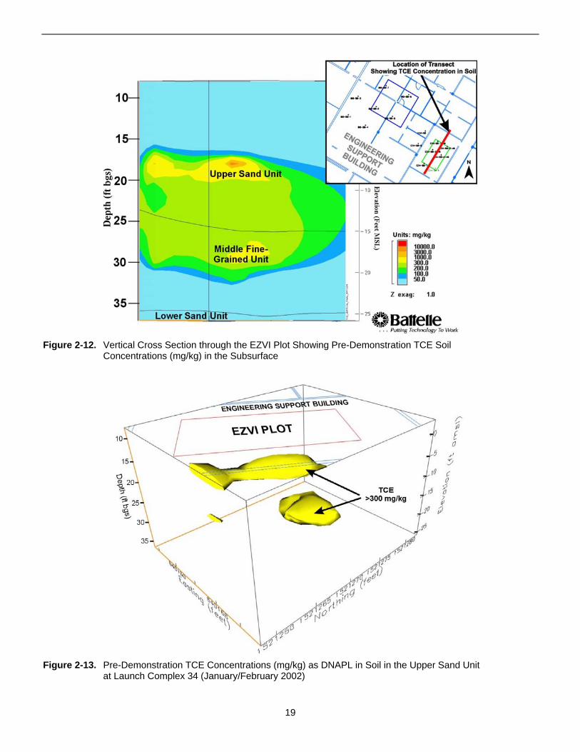
Figure 2-12. Vertical Cross Section through the EZVI Plot Showing Pre-Demonstration TCE Soil Concentrations (mg/kg) in the Subsurface

Figure 2-13. Pre-Demonstration TCE Concentrations (mg/kg) as DNAPL in Soil in the Upper Sand Unit at Launch Complex 34 (January/February 2002)

19

2.4 Aquifer Quality at the Site

Appendix A.3 lists the various aquifer parameters measured and the standard methods used to analyze them. Appendix D contains the results of the pre-demonstration groundwater analysis. Pre-demonstration groundwater field parameters were measured in several wells in the demonstration area in March 2002. The pH was relatively constant with depth, and ranged from 6.4 to 6.8. Prior to the EZVI application, dissolved oxygen (DO) levels were measured at 1 mg/L or less in all of the wells that were sampled, indicating that the aquifer was anaerobic. Oxidation-reduction potential (ORP) from all the sampled wells ranged from +15 to +148 millivolts (mV). The levels for total organic carbon (TOC) were relatively low and varied from 0.9 to 1.7% of dry soil weight, which indicates that microbes degrading TCE at the site used available TOC as a carbon source.

Inorganic groundwater parameters in the surficial aquifer were measured in March 2002 at the performance moni­toring wells in the Upper Sand Unit to determine the pre-demonstration quality of the groundwater in the target area.

• Total dissolved solids (TDS) concentrations increased sharply with depth, suggesting that the water becomes more brackish with depth. The TDS levels ranged from 947 to 1,670 mg/L. Chloride concentrations ranged from 177 to 848 mg/L and increased sharply with depth, indicating some saltwater intrusion in the deeper layers. These high

levels of chloride made it difficult to determine the extent to which additional chloride byproducts were formed after treatment.

• Alkalinity levels ranged from 222 to 475 mg/L, with no discernable trend with depth.

• Dissolved iron concentrations ranged from 1.1 to 27 mg/L in the groundwater, and decreased with depth. Total iron concentrations ranged from 1.2 to 22 mg/L in groundwater. Both dissolved and total iron concentrations in groundwater were highest in the Upper Sand Unit.

• Dissolved silica concentrations ranged from 20.4 to 54.6 mg/L, and increased with depth.

• Calcium concentrations ranged from 60 to 935 mg/L, with no discernible trend with depth. Magnesium concentrations ranged from 15 to 72 mg/L, and increased with increasing depth.

• Sodium concentrations were between 34 and 443 mg/L, and increased with depth. Potassium concentrations ranged from 17 to 299 mg/L, and decreased with depth.

• The changes in microbial characteristics of the aquifer were determined by comparing the biological oxygen demand (BOD) and dissolved methane gas concentrations in groundwater samples collected before and after the EZVI dem­onstration. BOD levels in the pre-demonstration groundwater samples ranged from <3 to 10 mg/L.

20

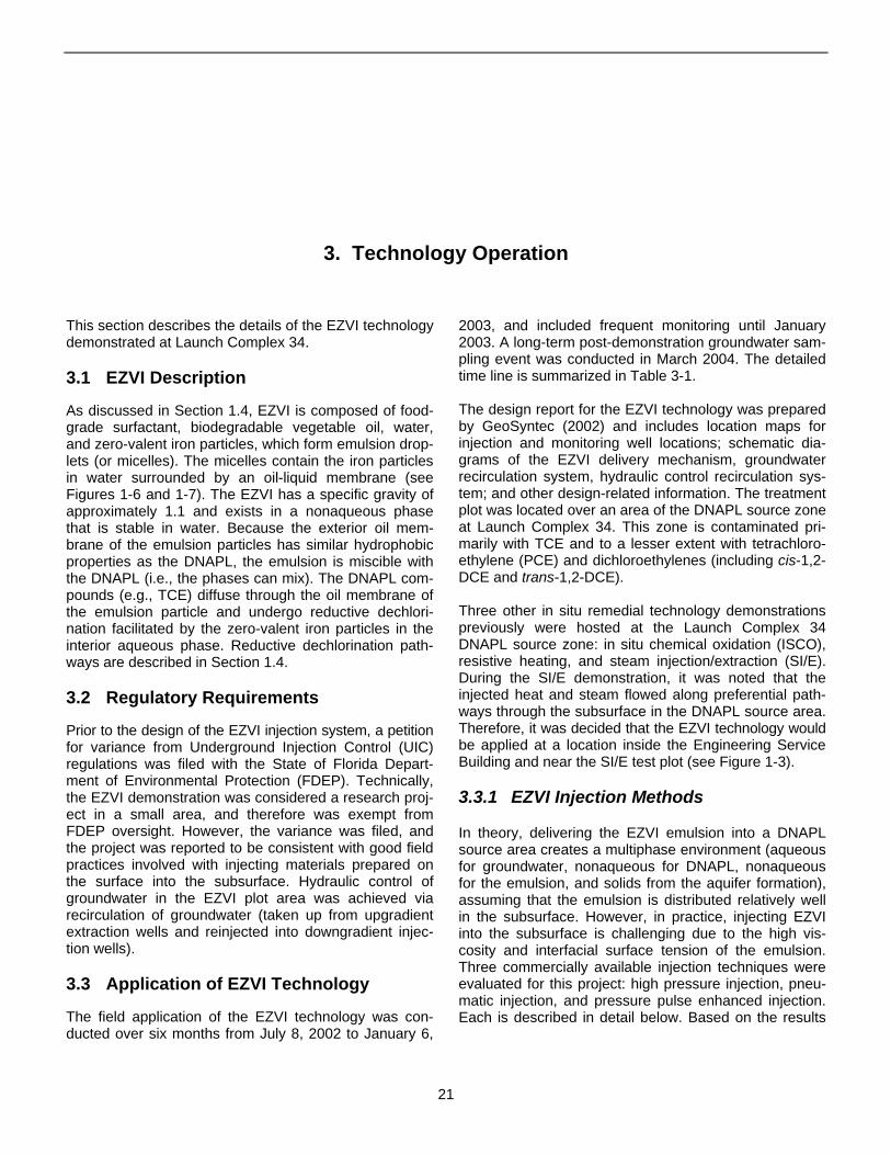
3. Technology Operation

This section describes the details of the EZVI technology demonstrated at Launch Complex 34.

3.1 EZVI Description

As discussed in Section 1.4, EZVI is composed of food-grade surfactant, biodegradable vegetable oil, water, and zero-valent iron particles, which form emulsion drop­lets (or micelles). The micelles contain the iron particles in water surrounded by an oil-liquid membrane (see Figures 1-6 and 1-7). The EZVI has a specific gravity of approximately 1.1 and exists in a nonaqueous phase that is stable in water. Because the exterior oil mem­brane of the emulsion particles has similar hydrophobic properties as the DNAPL, the emulsion is miscible with the DNAPL (i.e., the phases can mix). The DNAPL com­pounds (e.g., TCE) diffuse through the oil membrane of the emulsion particle and undergo reductive dechlori­nation facilitated by the zero-valent iron particles in the interior aqueous phase. Reductive dechlorination path­ways are described in Section 1.4.

3.2 Regulatory Requirements

Prior to the design of the EZVI injection system, a petition for variance from Underground Injection Control (UIC) regulations was filed with the State of Florida Depart­ment of Environmental Protection (FDEP). Technically, the EZVI demonstration was considered a research proj­ect in a small area, and therefore was exempt from FDEP oversight. However, the variance was filed, and the project was reported to be consistent with good field practices involved with injecting materials prepared on the surface into the subsurface. Hydraulic control of groundwater in the EZVI plot area was achieved via recirculation of groundwater (taken up from upgradient extraction wells and reinjected into downgradient injec­tion wells).

3.3 Application of EZVI Technology

The field application of the EZVI technology was con­ducted over six months from July 8, 2002 to January 6,

2003, and included frequent monitoring until January 2003. A long-term post-demonstration groundwater sam­pling event was conducted in March 2004. The detailed time line is summarized in Table 3-1.

The design report for the EZVI technology was prepared by GeoSyntec (2002) and includes location maps for injection and monitoring well locations; schematic dia­grams of the EZVI delivery mechanism, groundwater recirculation system, hydraulic control recirculation sys­tem; and other design-related information. The treatment plot was located over an area of the DNAPL source zone at Launch Complex 34. This zone is contaminated pri­marily with TCE and to a lesser extent with tetrachloro­ethylene (PCE) and dichloroethylenes (including cis-1,2­DCE and trans-1,2-DCE).

Three other in situ remedial technology demonstrations previously were hosted at the Launch Complex 34 DNAPL source zone: in situ chemical oxidation (ISCO), resistive heating, and steam injection/extraction (SI/E). During the SI/E demonstration, it was noted that the injected heat and steam flowed along preferential path­ways through the subsurface in the DNAPL source area. Therefore, it was decided that the EZVI technology would be applied at a location inside the Engineering Service Building and near the SI/E test plot (see Figure 1-3).

3.3.1 EZVI Injection Methods

In theory, delivering the EZVI emulsion into a DNAPL source area creates a multiphase environment (aqueous for groundwater, nonaqueous for DNAPL, nonaqueous for the emulsion, and solids from the aquifer formation), assuming that the emulsion is distributed relatively well in the subsurface. However, in practice, injecting EZVI into the subsurface is challenging due to the high vis­cosity and interfacial surface tension of the emulsion. Three commercially available injection techniques were evaluated for this project: high pressure injection, pneu­matic injection, and pressure pulse enhanced injection. Each is described in detail below. Based on the results

21

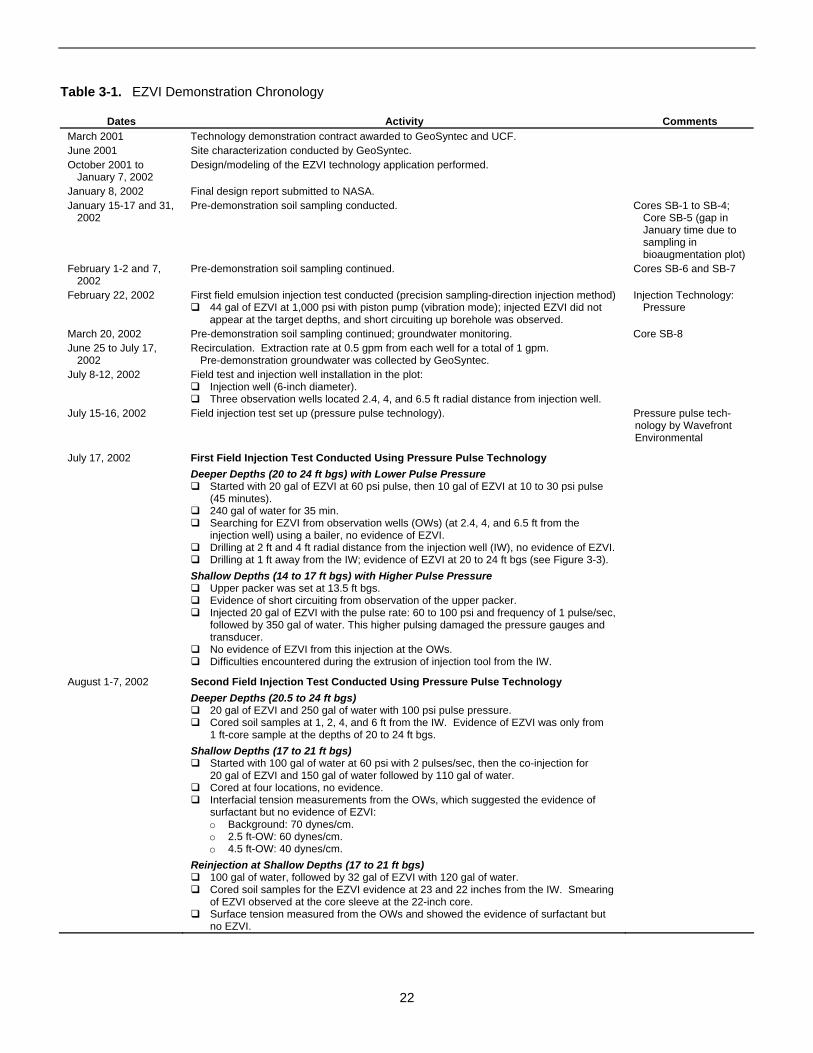
Dates Activity Comments March 2001 Technology demonstration contract awarded to GeoSyntec and UCF. June 2001 Site characterization conducted by GeoSyntec. October 2001 to Design/modeling of the EZVI technology application performed.

January 7, 2002January 8, 2002 Final design report submitted to NASA. January 15-17 and 31, Pre-demonstration soil sampling conducted. Cores SB-1 to SB-4;

2002 Core SB-5 (gap in January time due to sampling in bioaugmentation plot)

February 1-2 and 7, Pre-demonstration soil sampling continued. Cores SB-6 and SB-7 2002

February 22, 2002 First field emulsion injection test conducted (precision sampling-direction injection method) Injection Technology: � 44 gal of EZVI at 1,000 psi with piston pump (vibration mode); injected EZVI did not Pressure

appear at the target depths, and short circuiting up borehole was observed. March 20, 2002 Pre-demonstration soil sampling continued; groundwater monitoring. Core SB-8 June 25 to July 17, Recirculation. Extraction rate at 0.5 gpm from each well for a total of 1 gpm.

2002 Pre-demonstration groundwater was collected by GeoSyntec. July 8-12, 2002 Field test and injection well installation in the plot:

� Injection well (6-inch diameter). � Three observation wells located 2.4, 4, and 6.5 ft radial distance from injection well.

July 15-16, 2002 Field injection test set up (pressure pulse technology). Pressure pulse tech­nology by Wavefront Environmental

July 17, 2002 First Field Injection Test Conducted Using Pressure Pulse Technology Deeper Depths (20 to 24 ft bgs) with Lower Pulse Pressure � Started with 20 gal of EZVI at 60 psi pulse, then 10 gal of EZVI at 10 to 30 psi pulse

(45 minutes). � 240 gal of water for 35 min. � Searching for EZVI from observation wells (OWs) (at 2.4, 4, and 6.5 ft from the

injection well) using a bailer, no evidence of EZVI. � Drilling at 2 ft and 4 ft radial distance from the injection well (IW), no evidence of EZVI. � Drilling at 1 ft away from the IW; evidence of EZVI at 20 to 24 ft bgs (see Figure 3-3). Shallow Depths (14 to 17 ft bgs) with Higher Pulse Pressure � Upper packer was set at 13.5 ft bgs. � Evidence of short circuiting from observation of the upper packer. � Injected 20 gal of EZVI with the pulse rate: 60 to 100 psi and frequency of 1 pulse/sec,

followed by 350 gal of water. This higher pulsing damaged the pressure gauges and transducer.

� No evidence of EZVI from this injection at the OWs. � Difficulties encountered during the extrusion of injection tool from the IW.

August 1-7, 2002 Second Field Injection Test Conducted Using Pressure Pulse Technology Deeper Depths (20.5 to 24 ft bgs) � 20 gal of EZVI and 250 gal of water with 100 psi pulse pressure. � Cored soil samples at 1, 2, 4, and 6 ft from the IW. Evidence of EZVI was only from

1 ft-core sample at the depths of 20 to 24 ft bgs. Shallow Depths (17 to 21 ft bgs) � Started with 100 gal of water at 60 psi with 2 pulses/sec, then the co-injection for

20 gal of EZVI and 150 gal of water followed by 110 gal of water. � Cored at four locations, no evidence. � Interfacial tension measurements from the OWs, which suggested the evidence of

surfactant but no evidence of EZVI: o Background: 70 dynes/cm. o 2.5 ft-OW: 60 dynes/cm. o 4.5 ft-OW: 40 dynes/cm.

Reinjection at Shallow Depths (17 to 21 ft bgs) � 100 gal of water, followed by 32 gal of EZVI with 120 gal of water. � Cored soil samples for the EZVI evidence at 23 and 22 inches from the IW. Smearing

of EZVI observed at the core sleeve at the 22-inch core. � Surface tension measured from the OWs and showed the evidence of surfactant but

no EZVI.

Table 3-1. EZVI Demonstration Chronology

22

Table 3-1. EZVI Demonstration Schedule (continued)

Dates Activity Comments August 8-13, 2002 EZVI Injection Conducted (see Table 3-2 and Figure 3-3). August 20-21, 2002 Groundwater sampling conducted during the monitoring. August 24-29, 2002 Groundwater extracted from PA-23 at 0.3 gpm. September 13-25,

2002 Groundwater extracted from PA-23 at 0.3 gpm.

October 8-9, 2002 Simplified post-demonstration soil sampling. Cores SB-203, -204, -207 to -210

November, 2002 Post-demonstration characterization (soil and groundwater). Cores SB-301 to -304; -307 to -308

December 12, 2002 to January 6, 2003

March 8, 2004

Groundwater recirculation from the injection wells to extraction wells at 0.5 gpm per well for total of 1 gpm.

Final round of groundwater samples collected (January 6) by GeoSyntec. Groundwater sampling conducted in select monitoring wells to collect long-term post-

demonstration observational data. PA-23, PA-24S, PA­

25S, EIW-1, EEW-1

of field tests, one injection technique was selected for use during the demonstration.

3.3.1.1 Direct Injection

The first injection technology evaluated was direct injec­tion with high pressure. A direct-push drilling rig (Preci­sion Sampling) was used to advance a drilling rod to a desired depth, and then the outer casing of the driving rod was lifted in order to expose a screen to the forma­tion. The emulsion then was injected downward through the rod and sideways through the screen.

The initial plans for EZVI injection were involved with the injection at multiple locations and multiple depths in the treatment zone of the EZVI plot using a direct-push drill rig equipped with a “top-to-bottom” injection tool and an injection pump. The vertical and horizontal spacing of the injection points were to be determined by the limited space of the plot.

A direct-push hydraulic drill rig was used to deliver the EZVI into the subsurface over three discrete adjacent 2-ft intervals. The EZVI was injected over a 6-ft interval to simplify monitoring of the subsurface distribution of EZVI.

During the field test, the hydraulic rig advanced a custom top-down injection slide tool assembly attached to a direct-push, hollow 1.5-inch-outside diameter (O.D.) drive rod. The injection tip was comprised of a customized Geoprobe® open interval, 360-degree­circumference, hole-perforated drive stem sealed within the drive rods. The assembled slide tool was advanced to the top of the injection interval using a standard drive cap. An injection pull cap was connected to the top probe rod and the tool string was withdrawn 4 to 6 inches to expose the injection ports in the drive-point. The upper portion of the probe rod, which is pulled back

to expose the injection ports seals off the zones above the injection ports, was intended to function as a packer and minimize short-circuiting of the emulsion. The injec­tion tip was advanced to approximately 2 ft below the water table and the first injection of EZVI was initiated. The EZVI emulsion was injected using a GS2000 grout pump (reciprocating-type piston pump) capable of providing operating pressures up to 1,500 pounds per square inch (psi). The EZVI emulsion was gravity fed to the pump from a hopper and pumped through high pressure hose to the hollow drill stem and down to the injection tip. After the target volume of EZVI had been pumped at the first injection depth, the injection tip was advanced 2 ft and the injection process was repeated (GeoSyntec, 2003).

Before the EZVI emulsion was injected at the third depth it became obvious that the emulsion was short-circuiting up the drill stem and evidenced both at the ground surface and over the interface of water table and unsat­urated interval. The injection was repeated at two differ­ent locations with varying injection pressures but the EZVI emulsion continued to travel vertically up the injec­tion tool rather than out into the aquifer formation.

It was determined that the direct injection method was not suitable for the demonstration of EZVI injection.

3.3.1.2 Liquid Atomization Injection

The second injection technology evaluated was the Liquid Atomization Injection (LAI) pneumatic injection technique by ARS Technologies. This technique is more effective at injecting gases or “aerosols” into the sub­surface. The technique involves using nitrogen gas to atomize low-kinetic-energy, high-viscosity fluids into high-energy aerosols, and then using a multiphase injec­tion system to distribute the material into the subsurface.

23

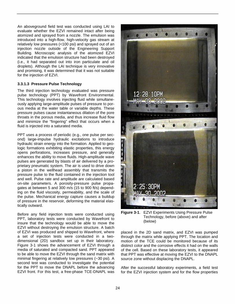
An aboveground field test was conducted using LAI to evaluate whether the EZVI remained intact after being atomized and sprayed from a nozzle. The emulsion was introduced into a high-flow, high-velocity gas stream at relatively low pressures (<100 psi) and sprayed out of an injection nozzle outside of the Engineering Support Building. Microscopic analysis of the atomized EZVI indicated that the emulsion structure had been destroyed (i.e., it had separated out into iron particulate and oil droplets). Although the LAI technique is very innovative and promising, it was determined that it was not suitable for the injection of EZVI.

3.3.1.3 Pressure Pulse Technology

The third injection technology evaluated was pressure pulse technology (PPT) by Wavefront Environmental. This technology involves injecting fluid while simultane­ously applying large-amplitude pulses of pressure to por­ous media at the water table or variable depths. These pressure pulses cause instantaneous dilation of the pore throats in the porous media, and thus increase fluid flow and minimize the “fingering” effect that occurs when a fluid is injected into a saturated media.

PPT uses a process of periodic (e.g., one pulse per sec­ond) large-impulse hydraulic excitations to introduce hydraulic strain energy into the formation. Applied to geo­logic formations exhibiting elastic properties, this energy opens perforations, increases pressure, and generally enhances the ability to move fluids. High-amplitude wave pulses are generated by blasts of air delivered by a pro­prietary pneumatic system. The air is used to drive down a piston in the wellhead assembly that transmits the pressure pulse to the fluid contained in the injection tool and well. Pulse rate and amplitude are calculated based on-site parameters. A porosity-pressure pulse propa­gates at between 5 and 300 m/s (15 to 900 ft/s) depend­ing on the fluid viscosity, permeability, and the scale of the pulse. Mechanical energy capture causes a buildup of pressure in the reservoir, deforming the material elas­tically outward.

Before any field injection tests were conducted using PPT, laboratory tests were conducted by Wavefront to insure that the technology would be able to move the EZVI without destroying the emulsion structure. A batch of EZVI was produced and shipped to Wavefront, where a set of injection tests were conducted in a two-dimensional (2D) sandbox set up in their laboratory. Figure 3-1 shows the advancement of EZVI through a media of saturated and compacted sand. PPT appeared to be able to move the EZVI through the sand matrix with minimal fingering at relatively low pressures (~30 psi). A second test was conducted to investigate the potential for the PPT to move the DNAPL before the advancing EZVI front. For this test, a free-phase TCE-DNAPL was

Figure 3-1. EZVI Experiments Using Pressure Pulse Technology, before (above) and after (below)

placed in the 2D sand matrix, and EZVI was pumped through the matrix while applying PPT. The location and motion of the TCE could be monitored because of its distinct color and the corrosive effects it had on the walls of the cell. Based on these laboratory tests, it appeared that PPT was effective at moving the EZVI to the DNAPL source zone without displacing the DNAPL.

After the successful laboratory experiments, a field test for the EZVI injection system and for the flow properties

24

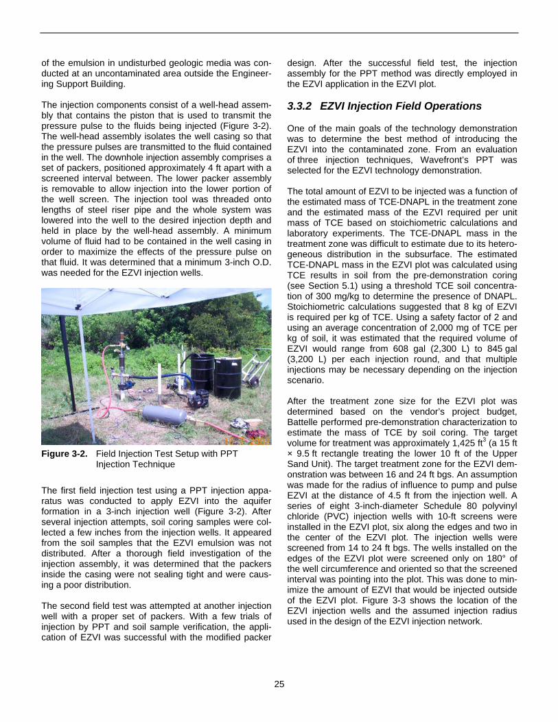
of the emulsion in undisturbed geologic media was con­ducted at an uncontaminated area outside the Engineer­ing Support Building.

The injection components consist of a well-head assem­bly that contains the piston that is used to transmit the pressure pulse to the fluids being injected (Figure 3-2). The well-head assembly isolates the well casing so that the pressure pulses are transmitted to the fluid contained in the well. The downhole injection assembly comprises a set of packers, positioned approximately 4 ft apart with a screened interval between. The lower packer assembly is removable to allow injection into the lower portion of the well screen. The injection tool was threaded onto lengths of steel riser pipe and the whole system was lowered into the well to the desired injection depth and held in place by the well-head assembly. A minimum volume of fluid had to be contained in the well casing in order to maximize the effects of the pressure pulse on that fluid. It was determined that a minimum 3-inch O.D. was needed for the EZVI injection wells.

Figure 3-2. Field Injection Test Setup with PPT Injection Technique

The first field injection test using a PPT injection appa­ratus was conducted to apply EZVI into the aquifer formation in a 3-inch injection well (Figure 3-2). After several injection attempts, soil coring samples were col­lected a few inches from the injection wells. It appeared from the soil samples that the EZVI emulsion was not distributed. After a thorough field investigation of the injection assembly, it was determined that the packers inside the casing were not sealing tight and were caus­ing a poor distribution.

The second field test was attempted at another injection well with a proper set of packers. With a few trials of injection by PPT and soil sample verification, the appli­cation of EZVI was successful with the modified packer

design. After the successful field test, the injection assembly for the PPT method was directly employed in the EZVI application in the EZVI plot.

3.3.2 EZVI Injection Field Operations

One of the main goals of the technology demonstration was to determine the best method of introducing the EZVI into the contaminated zone. From an evaluation of three injection techniques, Wavefront’s PPT was selected for the EZVI technology demonstration.

The total amount of EZVI to be injected was a function of the estimated mass of TCE-DNAPL in the treatment zone and the estimated mass of the EZVI required per unit mass of TCE based on stoichiometric calculations and laboratory experiments. The TCE-DNAPL mass in the treatment zone was difficult to estimate due to its hetero­geneous distribution in the subsurface. The estimated TCE-DNAPL mass in the EZVI plot was calculated using TCE results in soil from the pre-demonstration coring (see Section 5.1) using a threshold TCE soil concentra­tion of 300 mg/kg to determine the presence of DNAPL. Stoichiometric calculations suggested that 8 kg of EZVI is required per kg of TCE. Using a safety factor of 2 and using an average concentration of 2,000 mg of TCE per kg of soil, it was estimated that the required volume of EZVI would range from 608 gal (2,300 L) to 845 gal (3,200 L) per each injection round, and that multiple injections may be necessary depending on the injection scenario.

After the treatment zone size for the EZVI plot was determined based on the vendor’s project budget, Battelle performed pre-demonstration characterization to estimate the mass of TCE by soil coring. The target volume for treatment was approximately 1,425 ft3 (a 15 ft × 9.5 ft rectangle treating the lower 10 ft of the Upper Sand Unit). The target treatment zone for the EZVI dem­onstration was between 16 and 24 ft bgs. An assumption was made for the radius of influence to pump and pulse EZVI at the distance of 4.5 ft from the injection well. A series of eight 3-inch-diameter Schedule 80 polyvinyl chloride (PVC) injection wells with 10-ft screens were installed in the EZVI plot, six along the edges and two in the center of the EZVI plot. The injection wells were screened from 14 to 24 ft bgs. The wells installed on the edges of the EZVI plot were screened only on 180° of the well circumference and oriented so that the screened interval was pointing into the plot. This was done to min­imize the amount of EZVI that would be injected outside of the EZVI plot. Figure 3-3 shows the location of the EZVI injection wells and the assumed injection radius used in the design of the EZVI injection network.

25

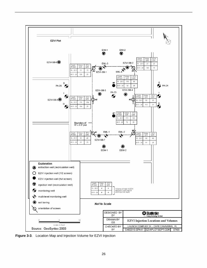
Figure 3-3. Location Map and Injection Volume for EZVI Injection

26

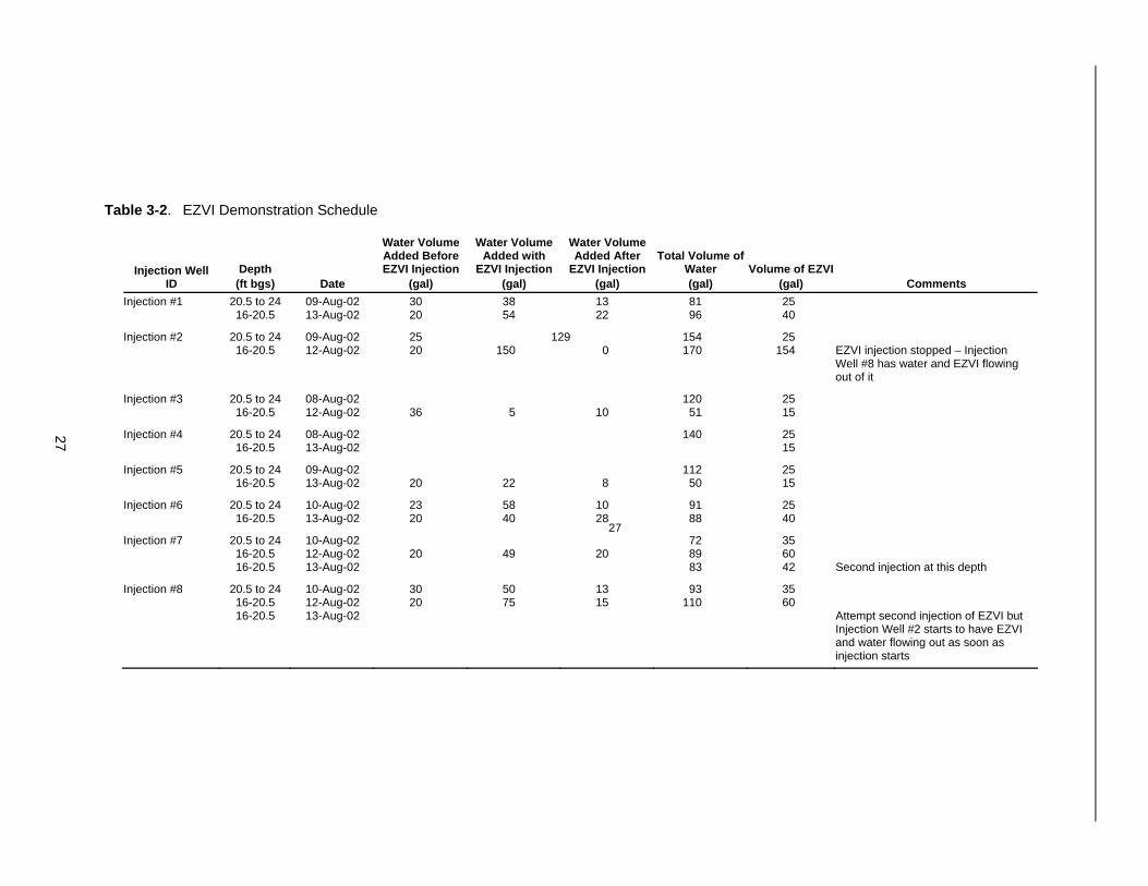
27

Table 3-2. EZVI Demonstration Schedule

Injection Well ID

Depth (ft bgs) Date

Water Volume Added Before EZVI Injection

(gal)

Water Volume Added with

EZVI Injection (gal)

Water Volume Added After

EZVI Injection (gal)

Total Volume of Water (gal)

Volume of EZVI (gal) Comments

Injection #1 20.5 to 24 16-20.5

09-Aug-02 13-Aug-02

30 20

38 54

13 22

81 96

25 40

Injection #2 20.5 to 24 16-20.5

09-Aug-02 12-Aug-02

25 20 150

129 0

154 170

25 154 EZVI injection stopped – Injection

Well #8 has water and EZVI flowing out of it

Injection #3 20.5 to 24 16-20.5

08-Aug-02 12-Aug-02 36 5 10

120 51

25 15

Injection #4 20.5 to 24 16-20.5

08-Aug-02 13-Aug-02

140

27

25 15

Injection #5 20.5 to 24 16-20.5

09-Aug-02 13-Aug-02 20 22 8

112 50

25 15

Injection #6 20.5 to 24 16-20.5

10-Aug-02 13-Aug-02

23 20

58 40

10 28

91 88

25 40

Injection #7 20.5 to 24 16-20.5 16-20.5

10-Aug-02 12-Aug-02 13-Aug-02

20 49 20 72 89 83

35 60 42 Second injection at this depth

Injection #8 20.5 to 24 16-20.5 16-20.5

10-Aug-02 12-Aug-02 13-Aug-02

30 20

50 75

13 15

93 110

35 60

Attempt second injection of EZVI but Injection Well #2 starts to have EZVI and water flowing out as soon as injection starts

Before injecting the EZVI emulsion into the test plot, a second injection test with the PPT system was con­ducted outside Engineering Services Building. This test was conducted from August 1-7, 2002 (see Table 3-1.) The second field injection test demonstrated that the bottom packer was not properly working as designed: the lower packer inflation line was breaking when the packer was inflated. After the vendor fixed the bottom packer, 20 gal of EZVI was injected, followed by 250 gal of fresh water in order to chase EZVI at an injection pressure of 100 psi. Gauges confirmed that the injection was work­ing and that pressure was maintained on the packers, injection pulses, and wellhead. After the EZVI injection, several soil cores were collected at distances of 1, 2, 4, and 6 ft from the injection well. Only one soil core sam­ple saturated with EZVI was observed at 1 ft from the injection well at depths of 20 to 24 ft bgs. Given that co­injection with water appeared able to carry the EZVI emulsion into the formation, it was determined that fluidizing the subsurface prior to the EZVI injection was necessary. A rough calculation suggested that the injec­tion of 20 gal of EZVI filled more than 100% of the void space in the radius around the injection well at depths of 20 to 24 ft bgs. As a result of the oversaturated pore space, the EZVI was forced to move through preferential flows and channels towards the surface. Therefore, the injection technique was modified by first injecting water in the aquifer before and after the injection of EZVI. This modified injection technique was able to successfully overcome the difficulties of injecting a high-viscosity emulsion into subsurface.

During the EZVI application in the treatment plot, the co­injection ratio of EZVI and water was maintained between 1:2 to 1:4 at various depths as summarized in Table 3-2. The total volume of EZVI injected was approximately 661 gal and the total volume of water injected into the injection wells was 1,627 gal (Table 3-2). Approximately 2,300 gal of water and EZVI were injected into the EZVI plot. The details of the injection information are summarized in Figure 3-3 and Table 3-2.

3.4 Groundwater Control System

A groundwater control system was designed and installed to maintain the hydraulic groundwater control in the EZVI plot. The groundwater control system consists of (1) two injection wells (EIW-1 and EIW-2) upgradient and two extraction wells (EEW-1 and EEW-2) down-gradient of the EZVI plot, (2) an aboveground treatment system (see Figure 3-4) to treat VOCs prior to reinjec­tion, (3) the associated process piping, and (4) additional monitoring wells on the edges of the plot (EML-1 to -4), outside the plot (PA-24S/I/D and PA-25S/I/D), and inside the plot (PA-23).

The groundwater control system was used to maintain flow and hydraulic residence time in the EZVI plot. The technology vendor designed the specifics of the flow control based on Visual MODFLOW™ (GeoSyntec, 2002). The results indicated that a flowrate of 1 gallon per minute (gpm) was sufficient to maintain flow in the system. Extra care was taken to prevent any potential air from entering into the treatment system. Flowrate, pres­sure, and the extracted groundwater chemistry were monitored by the vendor.

The groundwater control system was operated during three separate periods: (1) pre-demonstration (June 25 to July 17, 2002) from EEW-1 and EEW-2, (2) during the demonstration (August 24 to 29 and September 13 to 25, 2002) from PA-23, and (3) post-demonstration (December 16, 2002 to January 6, 2003) from EEW-1 and EEW-2. Although the optimal flowrate indicated by the modeling results was 1 gpm, the recirculation system could be controlled with much lower flow. The technol­ogy vendor frequently calibrated and daily recorded the logs of the average groundwater extraction flowrates using a pressure transducer from various sample ports. The water level was measured and recorded several times a day with a data logger (GeoSyntec, 2003). Dur­ing every site visit (every other week), the following activities were performed to maintain the groundwater control system:

• Monitoring of the pressure drop across granulated activated carbon (GAC) tank filter cartridges

• Collection of water samples from the effluent sampling port of the GAC tanks

• Flowrate and pressure measurements

• Water level measurements

• Site inspection and engineering control

• Replacement of GAC tanks and filter cartridges when necessary

• Routine maintenance of the extraction pump.

Before the demonstration, the average flowrate was maintained at 0.5 gpm from both EEW wells (EEW-1 and EEW-2) downgradient from the EZVI plot. The flowrate was kept at average of 0.3 gpm from PA-23 prior to and during the demonstration. Approximately 7,000 gal was extracted from PA-23. Of those 7,000 gal, approximately 2,300 gal of water extracted from PA-23 were then co­injected with EZVI into the EZVI plot. The remaining water was reinjected into the injection wells (EIW-1 and EIW-2), which are approximately 20 ft upgradient of the plot, after the EZVI injection. This reinjection scheme would likely induce an inward gradient into the plot.

28

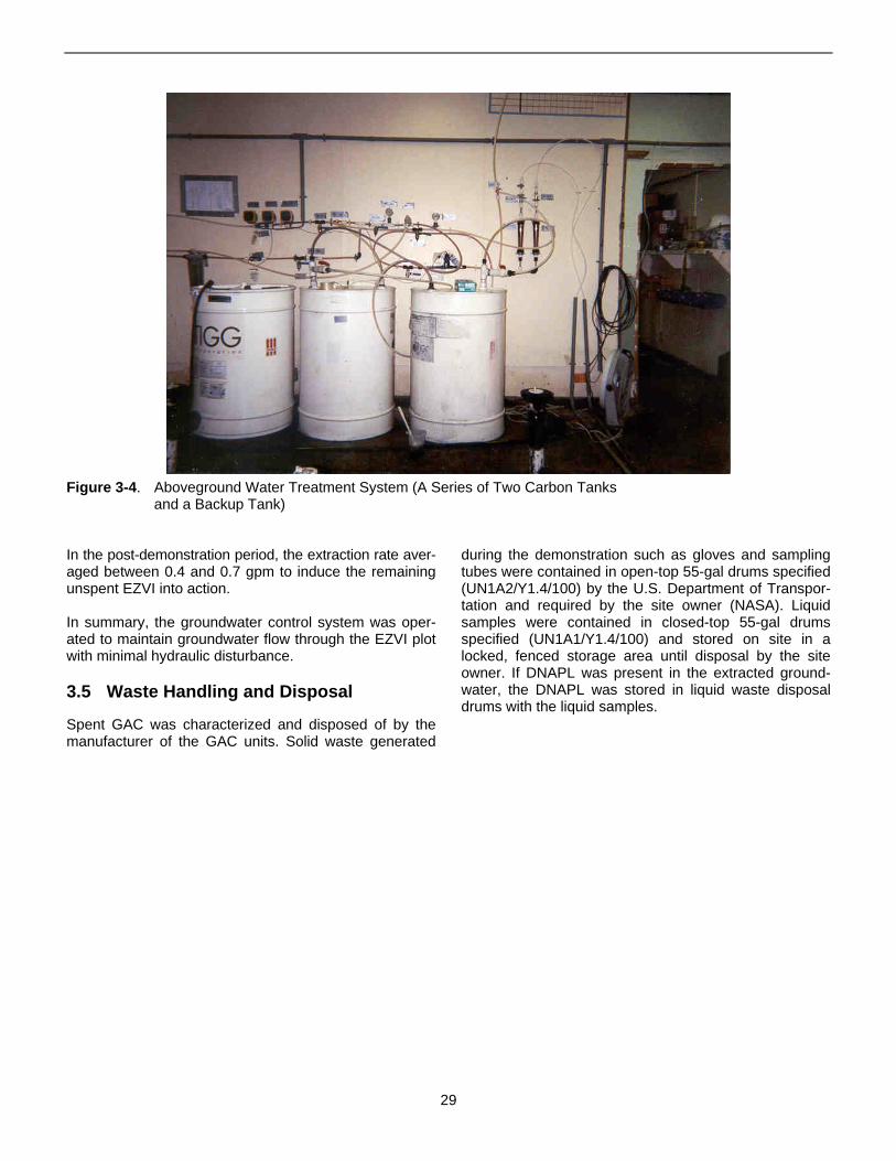
Figure 3-4. Aboveground Water Treatment System (A Series of Two Carbon Tanks and a Backup Tank)

In the post-demonstration period, the extraction rate aver­aged between 0.4 and 0.7 gpm to induce the remaining unspent EZVI into action.

In summary, the groundwater control system was oper­ated to maintain groundwater flow through the EZVI plot with minimal hydraulic disturbance.

3.5 Waste Handling and Disposal

Spent GAC was characterized and disposed of by the manufacturer of the GAC units. Solid waste generated

during the demonstration such as gloves and sampling tubes were contained in open-top 55-gal drums specified (UN1A2/Y1.4/100) by the U.S. Department of Transpor­tation and required by the site owner (NASA). Liquid samples were contained in closed-top 55-gal drums specified (UN1A1/Y1.4/100) and stored on site in a locked, fenced storage area until disposal by the site owner. If DNAPL was present in the extracted ground­water, the DNAPL was stored in liquid waste disposal drums with the liquid samples.

29

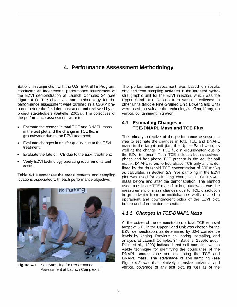
4. Performance Assessment Methodology

Battelle, in conjunction with the U.S. EPA SITE Program, conducted an independent performance assessment of the EZVI demonstration at Launch Complex 34 (see Figure 4-1). The objectives and methodology for the performance assessment were outlined in a QAPP pre­pared before the field demonstration and reviewed by all project stakeholders (Battelle, 2002a). The objectives of the performance assessment were to:

• Estimate the change in total TCE and DNAPL mass in the test plot and the change in TCE flux in groundwater due to the EZVI treatment;

• Evaluate changes in aquifer quality due to the EZVI treatment;

• Evaluate the fate of TCE due to the EZVI treatment;

• Verify EZVI technology operating requirements and costs.

Table 4-1 summarizes the measurements and sampling locations associated with each performance objective.

Figure 4-1. Soil Sampling for Performance Assessment at Launch Complex 34

The performance assessment was based on results obtained from sampling activities in the targeted hydro-stratigraphic unit for the EZVI injection, which was the Upper Sand Unit. Results from samples collected in other units (Middle Fine-Grained Unit, Lower Sand Unit) were used to evaluate the technology’s effect, if any, on vertical contaminant migration.

4.1 Estimating Changes in TCE-DNAPL Mass and TCE Flux

The primary objective of the performance assessment was to estimate the changes in total TCE and DNAPL mass in the target unit (i.e., the Upper Sand Unit), as well as the change in TCE flux in groundwater, due to the EZVI treatment. Total TCE includes both dissolved-phase and free-phase TCE present in the aquifer soil matrix. DNAPL refers to free-phase TCE only and is de­fined by the threshold TCE concentration of 300 mg/kg as calculated in Section 2.3. Soil sampling in the EZVI plot was used for estimating changes in TCE-DNAPL mass before and after the demonstration. The method used to estimate TCE mass flux in groundwater was the measurement of mass changes due to TCE dissolution in groundwater from the multichamber wells located in upgradient and downgradient sides of the EZVI plot, before and after the demonstration.

4.1.1 Changes in TCE-DNAPL Mass

At the outset of the demonstration, a total TCE removal target of 50% in the Upper Sand Unit was chosen for the EZVI demonstration, as determined by 80% confidence levels by kriging. Previous soil coring, sampling, and analysis at Launch Complex 34 (Battelle, 1999b; Eddy-Dilek et al., 1998) indicated that soil sampling was a viable technique for identifying the boundaries of the DNAPL source zone and estimating the TCE and DNAPL mass. The advantage of soil sampling (see Figure 4-2) was that relatively intensive horizontal and vertical coverage of any test plot, as well as of the

31

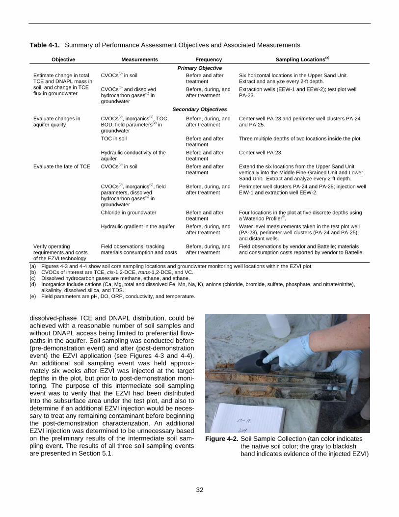
Table 4-1. Summary of Performance Assessment Objectives and Associated Measurements

Objective Measurements Frequency Sampling Locations(a)

Estimate change in total TCE and DNAPL mass in soil, and change in TCE flux in groundwater

Evaluate changes in aquifer quality

Evaluate the fate of TCE

Verify operating requirements and costs of the EZVI technology

Primary Objective CVOCs(b) in soil Before and after

treatment CVOCs(b) and dissolved Before, during, and hydrocarbon gases(c) in after treatment groundwater

Secondary Objectives

CVOCs(b), inorganics(d), TOC, Before, during, and BOD, field parameters(e) in after treatment groundwater TOC in soil Before and after

treatment Hydraulic conductivity of the Before and after aquifer treatment CVOCs(b) in soil Before and after

treatment

CVOCs(b), inorganics(d), field Before, during, and parameters, dissolved after treatment hydrocarbon gases(c) in groundwater Chloride in groundwater Before and after

treatment Hydraulic gradient in the aquifer Before, during, and

after treatment

Field observations, tracking Before, during, and materials consumption and costs after treatment

Six horizontal locations in the Upper Sand Unit. Extract and analyze every 2-ft depth. Extraction wells (EEW-1 and EEW-2); test plot well PA-23.

Center well PA-23 and perimeter well clusters PA-24 and PA-25.

Three multiple depths of two locations inside the plot.

Center well PA-23.

Extend the six locations from the Upper Sand Unit vertically into the Middle Fine-Grained Unit and Lower Sand Unit. Extract and analyze every 2-ft depth. Perimeter well clusters PA-24 and PA-25; injection well EIW-1 and extraction well EEW-2.

Four locations in the plot at five discrete depths using ®a Waterloo Profiler .

Water level measurements taken in the test plot well (PA-23), perimeter well clusters (PA-24 and PA-25), and distant wells. Field observations by vendor and Battelle; materials and consumption costs reported by vendor to Battelle.

(a)(b)(c) (d)

(e)

Figures 4-3 and 4-4 show soil core sampling locations and groundwater monitoring well locations within the EZVI plot. CVOCs of interest are TCE, cis-1,2-DCE, trans-1,2-DCE, and VC. Dissolved hydrocarbon gases are methane, ethane, and ethane. Inorganics include cations (Ca, Mg, total and dissolved Fe, Mn, Na, K), anions (chloride, bromide, sulfate, phosphate, and nitrate/nitrite), alkalinity, dissolved silica, and TDS. Field parameters are pH, DO, ORP, conductivity, and temperature.

dissolved-phase TCE and DNAPL distribution, could be achieved with a reasonable number of soil samples and without DNAPL access being limited to preferential flow-paths in the aquifer. Soil sampling was conducted before (pre-demonstration event) and after (post-demonstration event) the EZVI application (see Figures 4-3 and 4-4). An additional soil sampling event was held approxi­mately six weeks after EZVI was injected at the target depths in the plot, but prior to post-demonstration moni­toring. The purpose of this intermediate soil sampling event was to verify that the EZVI had been distributed into the subsurface area under the test plot, and also to determine if an additional EZVI injection would be neces­sary to treat any remaining contaminant before beginning the post-demonstration characterization. An additional EZVI injection was determined to be unnecessary based on the preliminary results of the intermediate soil sam­pling event. The results of all three soil sampling events are presented in Section 5.1.

Figure 4-2. Soil Sample Collection (tan color indicates the native soil color; the gray to blackish band indicates evidence of the injected EZVI)

32

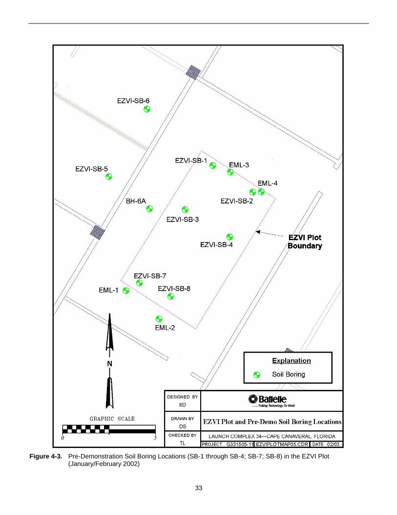
Figure 4-3. Pre-Demonstration Soil Boring Locations (SB-1 through SB-4; SB-7; SB-8) in the EZVI Plot (January/February 2002)

33

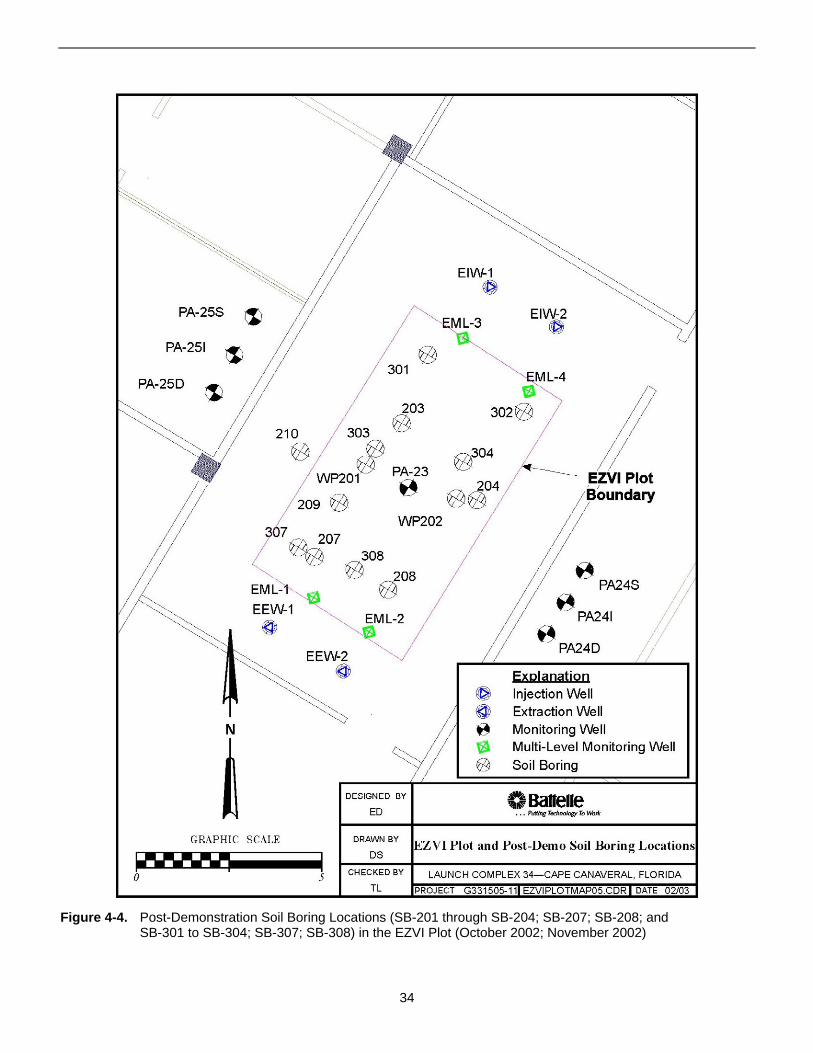
Figure 4-4. Post-Demonstration Soil Boring Locations (SB-201 through SB-204; SB-207; SB-208; and SB-301 to SB-304; SB-307; SB-308) in the EZVI Plot (October 2002; November 2002)

34

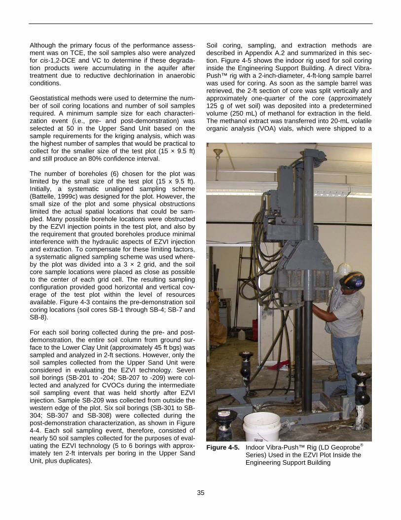
Although the primary focus of the performance assess­ment was on TCE, the soil samples also were analyzed for cis-1,2-DCE and VC to determine if these degrada­tion products were accumulating in the aquifer after treatment due to reductive dechlorination in anaerobic conditions.

Geostatistical methods were used to determine the num­ber of soil coring locations and number of soil samples required. A minimum sample size for each characteri­zation event (i.e., pre- and post-demonstration) was selected at 50 in the Upper Sand Unit based on the sample requirements for the kriging analysis, which was the highest number of samples that would be practical to collect for the smaller size of the test plot (15 × 9.5 ft) and still produce an 80% confidence interval.

The number of boreholes (6) chosen for the plot was limited by the small size of the test plot (15 x 9.5 ft). Initially, a systematic unaligned sampling scheme (Battelle, 1999c) was designed for the plot. However, the small size of the plot and some physical obstructions limited the actual spatial locations that could be sam­pled. Many possible borehole locations were obstructed by the EZVI injection points in the test plot, and also by the requirement that grouted boreholes produce minimal interference with the hydraulic aspects of EZVI injection and extraction. To compensate for these limiting factors, a systematic aligned sampling scheme was used where­by the plot was divided into a 3 × 2 grid, and the soil core sample locations were placed as close as possible to the center of each grid cell. The resulting sampling configuration provided good horizontal and vertical cov­erage of the test plot within the level of resources available. Figure 4-3 contains the pre-demonstration soil coring locations (soil cores SB-1 through SB-4; SB-7 and SB-8).

For each soil boring collected during the pre- and post-demonstration, the entire soil column from ground sur­face to the Lower Clay Unit (approximately 45 ft bgs) was sampled and analyzed in 2-ft sections. However, only the soil samples collected from the Upper Sand Unit were considered in evaluating the EZVI technology. Seven soil borings (SB-201 to -204; SB-207 to -209) were col­lected and analyzed for CVOCs during the intermediate soil sampling event that was held shortly after EZVI injection. Sample SB-209 was collected from outside the western edge of the plot. Six soil borings (SB-301 to SB­304; SB-307 and SB-308) were collected during the post-demonstration characterization, as shown in Figure 4-4. Each soil sampling event, therefore, consisted of nearly 50 soil samples collected for the purposes of eval­uating the EZVI technology (5 to 6 borings with approx­imately ten 2-ft intervals per boring in the Upper Sand Unit, plus duplicates).

Soil coring, sampling, and extraction methods are described in Appendix A.2 and summarized in this sec­tion. Figure 4-5 shows the indoor rig used for soil coring inside the Engineering Support Building. A direct Vibra-Push™ rig with a 2-inch-diameter, 4-ft-long sample barrel was used for coring. As soon as the sample barrel was retrieved, the 2-ft section of core was split vertically and approximately one-quarter of the core (approximately 125 g of wet soil) was deposited into a predetermined volume (250 mL) of methanol for extraction in the field. The methanol extract was transferred into 20-mL volatile organic analysis (VOA) vials, which were shipped to a

Figure 4-5. Indoor Vibra-Push™ Rig (LD Geoprobe®

Series) Used in the EZVI Plot Inside the Engineering Support Building

35

certified off-site laboratory for analysis. The sampling and extraction technique used at this site provided better coverage of a heterogeneously distributed contaminant distribution as compared to the more conventional meth­od of collecting and analyzing small soil samples at dis­crete depths, because the entire vertical depth of the soil column at the coring location could be analyzed. Prelimi­nary site characterization had shown that the vertical variability of the TCE distribution was greater than the horizontal variability, and this sampling and extraction method allowed continuous vertical coverage of the soil column (GeoSyntec, 2002). The efficiency of TCE recov­ery by this method (modified U.S. EPA Method 5035; see Appendix A.2) was evaluated through a series of tests conducted for the demonstration (Battelle, 2003). In these tests, a surrogate compound (1,1,1-trichloroethane [1,1,1-TCA]) was spiked into soil cores from the Launch Complex 34 aquifer, extracted, and analyzed. Replicate extractions and analysis of the spiked surrogate indicated a CVOC recovery efficiency between 84 and 113% (with an average recovery of 92%), which was considered sufficiently accurate for the demonstration.

Two data evaluation methods were used for estimating the change in TCE-DNAPL mass in the EZVI plot: linear interpolation by contouring, and kriging. The spatial vari­ability or spread of the TCE distribution in a DNAPL source zone typically is high, the reason being that small pockets of residual solvent may be distributed unevenly across the source region. The two methods address this spatial variability in different ways, and therefore the resulting mass removal estimates differ slightly. Because it is impractical to collect a sample from every single point in the EZVI plot and obtain a true TCE mass esti­mate for the plot, both methods address the practical difficulty of estimating the TCE concentrations at unsam­pled points by interpolating (estimating) between sam­pled points. The objective of both methods is to use the information from a limited sample set to make an infer­ence about the entire population (the entire plot or a stratigraphic unit).

4.1.2 Linear Interpolation by Contouring

Linear interpolation by contouring is the most straight­forward and intuitive method for estimating TCE concen­tration or mass in the entire plot, based on a limited number of sampled points. TCE concentrations are assumed to be linearly distributed between sampled points. A software program, such as EarthVision™, has an advantage over manual calculations in that it is easier to conduct the linear interpolation in three dimensions. In contouring, the only way to address the spatial variability of the TCE distribution is to collect as large a number of samples as is practical so that good coverage of the plot is obtained; the higher the sampling density, the smaller

the distances over which the data need to be interpo­lated.

For linear interpolation by contouring, input parameters must be adjusted to accommodate various references such as geology and sample size. Nearly 200 soil sam­ples were collected from the 17 coring locations in the plot during each event (pre-demonstration, intermediate, and post-demonstration), which was the highest number practical within the resources of this project. The number and distribution of these sampling points were deter­mined to obtain good representative coverage of the plot.

Linear interpolation by contouring using EarthVision™ software uses the same methodology that is used for drawing water level contour maps based on water level measurements at discrete locations in a region. The only difference with this software is that the TCE concen­trations are mapped in three dimensions to generate iso­concentration shells (i.e., volumes of soil that fall within a specified concentration range). The average TCE con­centration of each shell is multiplied by the volume of the shell (as estimated by the volumetric package in the software) and the bulk density of the soil (1.59 g/cm3) to estimate a TCE mass for each shell. The TCE mass in each region of interest (Upper Sand Unit, Middle-Fine-Grained Unit, or Lower Sand Unit) is obtained by adding up the portion of the shells contained in that region. The DNAPL mass is obtained by adding up the masses in only those shells that have TCE concentrations above 300 mg/kg. Contouring provides a single mass estimate for the region of interest.

4.1.3 Kriging

Kriging is a geostatistical interpolation method that takes into consideration the spatial correlations among the TCE data in making inferences about the TCE concen­trations at unsampled points. Spatial correlation analysis determines the extent to which TCE concentrations at various points in the plot are similar or different. Gener­ally, the degree to which TCE concentrations are similar or different is a function of distance and direction. Based on these correlations, kriging determines how the TCE concentrations at sampled points can be optimally weighted to infer the TCE concentrations/masses at unsampled points in the plot or the TCE mass in an entire region of interest (entire plot or stratigraphic unit). Kriging accounts for the uncertainty in each point esti­mate by calculating a standard error for the estimate. Therefore a range of TCE mass estimates is obtained instead of a single estimate; this range is defined by an average and a standard error or by a confidence interval. The confidence or level of significance required by the project objectives determines the width of this range. A

36

level of significance of 0.2 (or 80% confidence) was determined as necessary at the beginning of the dem­onstration (Battelle, 2002a).

4.1.4 Interpreting the Results of the Two Mass Removal Estimation Methods

The two data evaluation methods address the spatial variability of the TCE distribution in different ways and, therefore, the resulting mass removal estimates differ slightly between the two methods.

In both contouring and kriging, TCE mass removal is ac­counted for on an absolute basis; higher mass removal in a few high-TCE concentration portions of the plot can offset low mass removal in other portions of the plot, to infer a high level of mass removal. Kriging most likely provides a more informed inference of the TCE mass re­moval than contouring because it takes into account the spatial correlations in the TCE distribution and the uncer­tainties (error) associated with the estimates. The results in Section 5.1 show that contouring was able to over­come the spatial variability to a considerable extent and provide mass estimates that were generally in agree­ment with the ranges provided by kriging.

4.1.5 TCE Flux Measurements in Groundwater

In addition to estimating the changes in TCE-DNAPL mass, another primary objective of the performance assessment was to evaluate any changes in TCE flux in groundwater after the EZVI injection. Groundwater sam­ples were collected by the vendor from the multilevel samplers and the performance monitoring well network in the plot. The change in TCE flux is a measure of the reduction in activity of the DNAPL source (i.e., the strength of the DNAPL contribution to plume formation) brought about by the technology.

4.2 Evaluating Changes in Aquifer Quality

A secondary objective of the performance assessment was to evaluate any short-term changes in aquifer qual­ity due to the treatment. EZVI affects the contaminant and, to a lesser extent, the native aquifer characteristics. Pre- and post-demonstration measurements conducted to evaluate the short-term impacts of the technology application on the aquifer included:

• CVOC measurements in the groundwater inside the EZVI plot

• Field parameter measurements (pH, DO, ORP, temperature, and conductivity) in the groundwater

• Inorganic measurements (common cations and anions) in the groundwater

• TDS and 5-day BOD

• TOC measurements in the soil

• Hydraulic conductivity of the aquifer.

These measurements were conducted in the monitoring well within the plot and in the extraction wells and perim­eter wells surrounding the plot.

4.3 Evaluating the Fate of the TCE-DNAPL

Another secondary objective of the performance assess­ment was to evaluate the fate of TCE removed from the plot by the EZVI treatment. Possible pathways (or pro­cesses) for TCE removal include dehalogenation (de­struction of TCE) and migration from the EZVI plot (to outside the plot). Dehalogenation will be determined by the presence of TCE degradation products, including chloride. The amount of chloride generated during EZVI treatment was evaluated by collecting groundwater sam­ples with a Waterloo Profiler® inside the plot (see Figure 4-6), as well as from the performance monitoring wells. These pathways were evaluated by the following mea­surements:

• Chloride in groundwater (mineralization of CVOCs leads to formation of chloride) and other inorganic constituents in groundwater

• Alkalinity in groundwater (oxidation of CVOCs and native organic matter leads to formation of CO2 which, in a closed system, forms carbonate)

• Hydraulic gradients (injection of the emulsion creates gradients indicative of groundwater movement)

• Dissolved and total iron concentrations in the EZVI plot and surrounding wells

• Changes in dehalogenated byproducts (cis­1,2-DCE, VC, and ethenes)

• Impact on natural attenuation products (nitrate, sulfate) via the aerobic process.

37

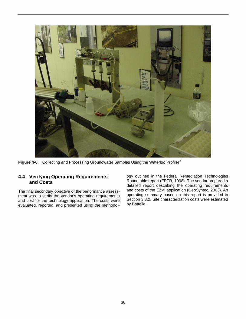
Figure 4-6. Collecting and Processing Groundwater Samples Using the Waterloo Profiler®

4.4 Verifying Operating Requirements ogy outlined in the Federal Remediation Technologies and Costs Roundtable report (FRTR, 1998). The vendor prepared a

detailed report describing the operating requirements The final secondary objective of the performance assess- and costs of the EZVI application (GeoSyntec, 2003). An ment was to verify the vendor’s operating requirements operating summary based on this report is provided in and cost for the technology application. The costs were Section 3.3.2. Site characterization costs were estimated evaluated, reported, and presented using the methodol- by Battelle.

38

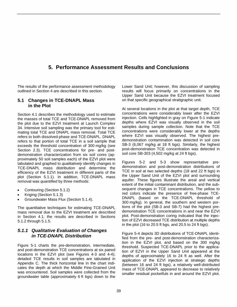
5. Performance Assessment Results and Conclusions

The results of the performance assessment methodology outlined in Section 4 are described in this section.

5.1 Changes in TCE-DNAPL Mass in the Plot

Section 4.1 describes the methodology used to estimate the masses of total TCE and TCE-DNAPL removed from the plot due to the EZVI treatment at Launch Complex 34. Intensive soil sampling was the primary tool for esti­mating total TCE and DNAPL mass removal. Total TCE refers to both dissolved-phase and TCE-DNAPL. DNAPL refers to that portion of total TCE in a soil sample that exceeds the threshold concentration of 300 mg/kg (see Section 2.3). TCE concentrations for pre- and post-demonstration characterization from six soil cores (ap­proximately 50 soil samples each) of the EZVI plot were tabulated and graphed to qualitatively identify changes in TCE-DNAPL mass distribution and determine the efficiency of the EZVI treatment in different parts of the plot (Section 5.1.1). In addition, TCE-DNAPL mass removal was quantified by three methods:

• Contouring (Section 5.1.2) • Kriging (Section 5.1.3) • Groundwater Mass Flux (Section 5.1.4).

The quantitative techniques for estimating TCE-DNAPL mass removal due to the EZVI treatment are described in Section 4.1; the results are described in Sections 5.1.2 through 5.1.5.

5.1.1 Qualitative Evaluation of Changes in TCE-DNAPL Distribution

Figure 5-1 charts the pre-demonstration, intermediate, and post-demonstration TCE concentrations at six paired locations in the EZVI plot (see Figures 4-3 and 4-4); detailed TCE results in soil samples are tabulated in Appendix C. The thick horizontal line in the chart indi­cates the depth at which the Middle Fine-Grained Unit was encountered. Soil samples were collected from the groundwater table (approximately 6 ft bgs) down to the

Lower Sand Unit; however, this discussion of sampling results will focus primarily on concentrations in the Upper Sand Unit because the EZVI treatment focused on that specific geographical stratigraphic unit.

At several locations in the plot at that target depth, TCE concentrations were considerably lower after the EZVI injection. Cells highlighted in gray on Figure 5-1 indicate depths where EZVI was visually observed in the soil samples during sample collection. Note that the TCE concentrations were considerably lower at the depths where EZVI was visually observed. The highest pre-demonstration contamination was detected in soil core SB-3 (6,067 mg/kg at 18 ft bgs). Similarly, the highest post-demonstration TCE concentration was detected in soil core SB-303 (4,502 mg/kg at 24 ft bgs).

Figures 5-2 and 5-3 show representative pre-demonstration and post-demonstration distributions of TCE in soil at two selected depths (18 and 22 ft bgs) in the Upper Sand Unit of the EZVI plot and surrounding aquifer. These figures illustrate the areal and vertical extent of the initial contaminant distribution, and the sub­sequent changes in TCE concentrations. The yellow to red colors indicate the presence of free-phase TCE­DNAPL (based on the TCE-DNAPL threshold of 300 mg/kg). In general, the southern and western por­tions of the plot (SB-3 and SB-7) had the highest pre-demonstration TCE concentrations in and near the EZVI plot. Post-demonstration coring indicated that the injec­tion of EZVI decreased TCE distribution at multiple depths in the plot (16 to 20.5 ft bgs, and 20.5 to 24 ft bgs).

Figure 5-4 depicts 3D distributions of TCE-DNAPL identi­fied from the pre- and post-demonstration characteriza­tion in the EZVI plot, and based on the 300 mg/kg threshold. Suspected TCE-DNAPL prior to the applica­tion of EZVI in the Upper Sand Unit appeared at the depths of approximately 16 to 24 ft as well. After the application of the EZVI injection at strategic depths (between 16 and 24 ft bgs), a relatively well-distributed mass of TCE-DNAPL appeared to decrease to relatively smaller residual pocketfuls in and around the EZVI plot.

39

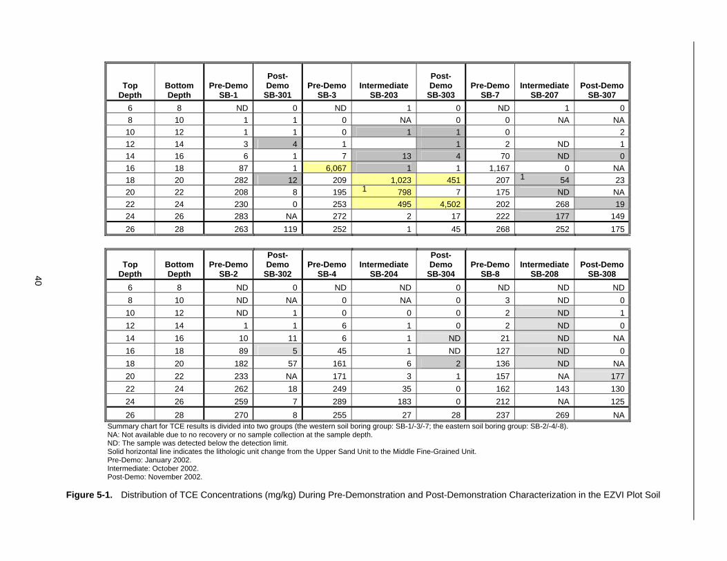
40

Top Depth

Bottom Depth

Pre-Demo SB-1

Post-Demo

SB-301 Pre-Demo

SB-3 Intermediate

SB-203

Post-Demo

SB-303 Pre-Demo

SB-7 Intermediate

SB-207 Post-Demo

SB-307 6 8 ND 0 ND 1 0 ND 1 0 8 10 1 1 0 NA 0 0 NA NA 10 12 1 1 0 1 1 0

1

2 12 14 3 4 1

1

1 2 ND 1 14 16 6 1 7 13 4 70 ND 0 16 18 87 1 6,067 1 1 1,167 0 NA 18 20 282 12 209 1,023 451 207 54 23 20 22 208 8 195 798 7 175 ND NA 22 24 230 0 253 495 4,502 202 268 19 24 26 283 NA 272 2 17 222 177 149 26 28 263 119 252 1 45 268 252 175

Top Depth

Bottom Depth

Pre-Demo SB-2

Post-Demo

SB-302 Pre-Demo

SB-4 Intermediate

SB-204

Post-Demo

SB-304 Pre-Demo

SB-8 Intermediate

SB-208 Post-Demo

SB-308 6 8 ND 0 ND ND 0 ND ND ND 8 10 ND NA 0 NA 0 3 ND 0 10 12 ND 1 0 0 0 2 ND 1 12 14 1 1 6 1 0 2 ND 0 14 16 10 11 6 1 ND 21 ND NA 16 18 89 5 45 1 ND 127 ND 0 18 20 182 57 161 6 2 136 ND NA 20 22 233 NA 171 3 1 157 NA 177 22 24 262 18 249 35 0 162 143 130 24 26 259 7 289 183 0 212 NA 125 26 28 270 8 255 27 28 237 269 NA

Summary chart for TCE results is divided into two groups (the western soil boring group: SB-1/-3/-7; the eastern soil boring group: SB-2/-4/-8). NA: Not available due to no recovery or no sample collection at the sample depth. ND: The sample was detected below the detection limit. Solid horizontal line indicates the lithologic unit change from the Upper Sand Unit to the Middle Fine-Grained Unit. Pre-Demo: January 2002. Intermediate: October 2002. Post-Demo: November 2002.

Figure 5-1. Distribution of TCE Concentrations (mg/kg) During Pre-Demonstration and Post-Demonstration Characterization in the EZVI Plot Soil

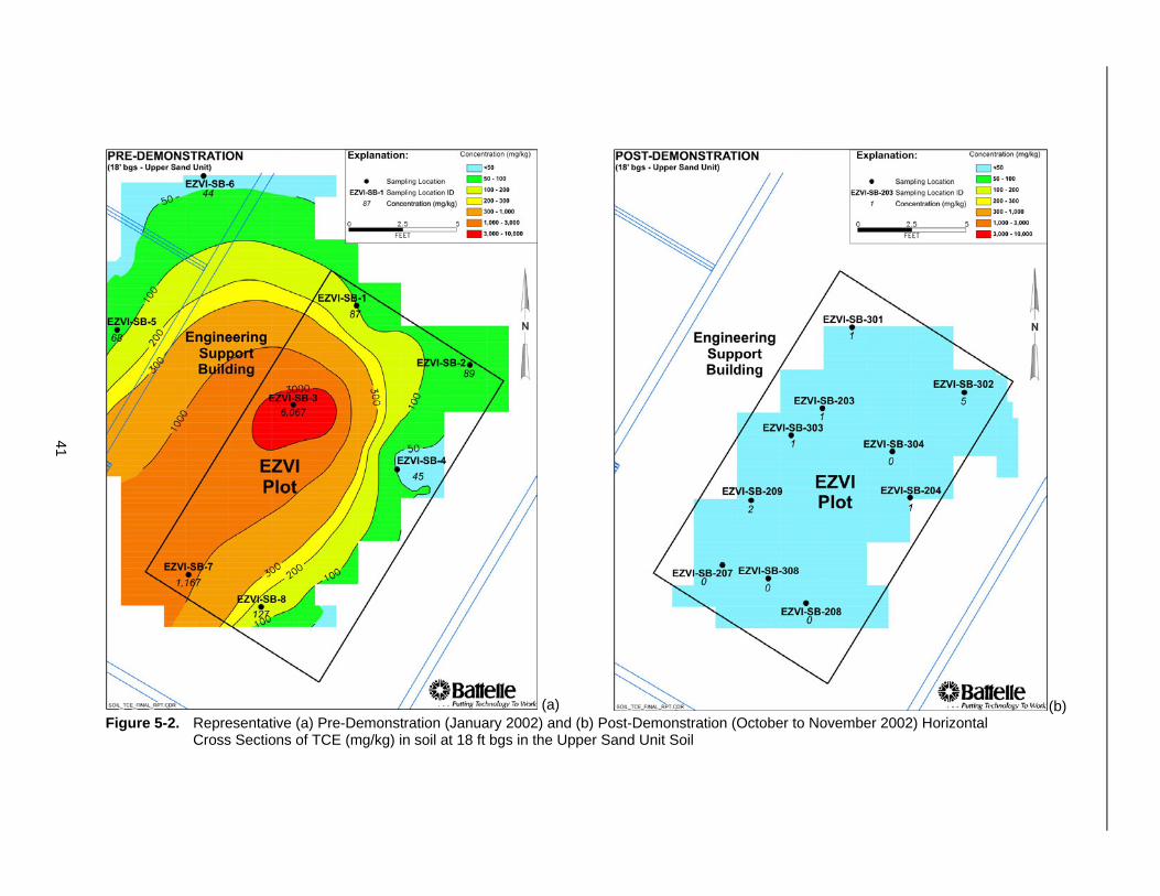
41

(a) (b) Figure 5-2. Representative (a) Pre-Demonstration (January 2002) and (b) Post-Demonstration (October to November 2002) Horizontal

Cross Sections of TCE (mg/kg) in soil at 18 ft bgs in the Upper Sand Unit Soil

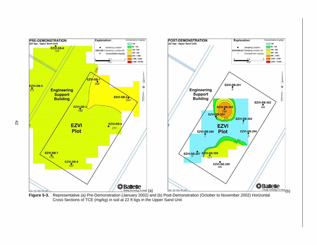
42

(a) (b) Figure 5-3. Representative (a) Pre-Demonstration (January 2002) and (b) Post-Demonstration (October to November 2002) Horizontal

Cross Sections of TCE (mg/kg) in soil at 22 ft bgs in the Upper Sand Unit

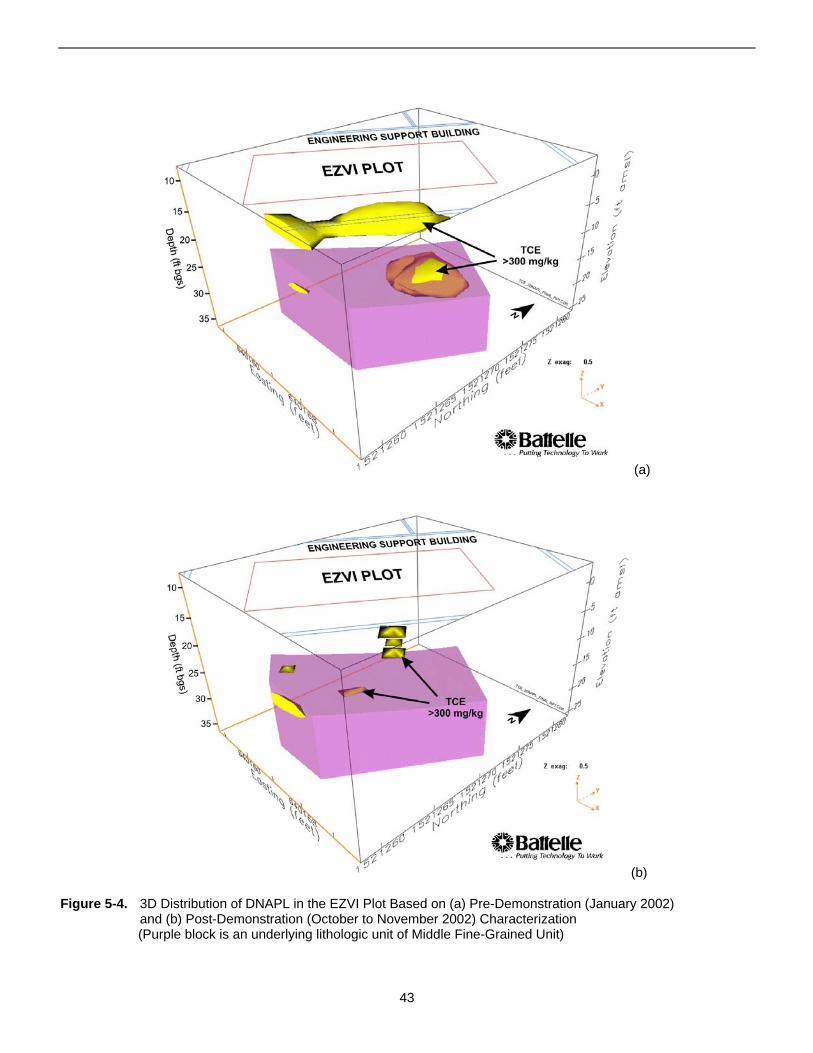
(a)

(b)

Figure 5-4. 3D Distribution of DNAPL in the EZVI Plot Based on (a) Pre-Demonstration (January 2002) and (b) Post-Demonstration (October to November 2002) Characterization (Purple block is an underlying lithologic unit of Middle Fine-Grained Unit)

43

Table 5-1. Estimated Total TCE and TCE-DNAPL Mass Reduction by Linear Interpolation

Pre-Demonstration Post-Demonstration Change in Mass (%) Total TCE Mass TCE-DNAPL Mass Total TCE Mass TCE-DNAPL Mass Total TCE-

Stratigraphic Unit (kg) (kg) (kg) (kg) TCE DNAPL Upper Sand Unit 17.8 3.8 2.6 0.6 86 84 Upper Sand Unit (without outlier)(a) 17.8 3.8 1.8 0.2 90 95 Middle Fine-Grained Unit(b) 11.8 1.5 6.9 0.5 N/A N/A Lower Sand Unit(b) 0.12 0.0 0.10 0.0 N/A N/A (a) The highest data point in the post-demonstration TCE data was dropped as a possible outlier. (b) The last two rows are shaded because any EZVI treatment of the Middle Fine-Grained Unit and Lower Sand Unit was incidental and these two

units were not targeted during the injection. N/A = not applicable.

One narrow pocket of significant DNAPL (4,502 mg/kg) was found in SB-303 at a depth of 22 to 24 ft bgs. Inter­estingly, EZVI also was observed at much shallower depths between 10 and 16 ft bgs where EZVI was not intentionally injected, but which reacted with TCE at the shallower depths (see Figure 5-1). This indicates that the EZVI was not evenly distributed laterally and ascended close to the groundwater table, suggesting that EZVI was likely pushed up during the injection.

In summary, a qualitative evaluation of the TCE-DNAPL changes indicates that the injection of EZVI treatment was able to achieve partial decrease of free-phase TCE­DNAPL in some parts of the plot. However, the efficiency of EZVI distribution may need to be improved in order to treat the remaining pockets of DNAPL.

5.1.2 TCE-DNAPL Mass Estimation by Linear Interpolation

Section 4.1.2 describes the use of linear interpolation or contouring to estimate pre- and post-demonstration TCE-DNAPL masses and calculate TCE-DNAPL mass changes within the plot. In this method, EarthVision™, a 3D contouring software, is used to group the TCE con­centration distribution in the EZVI plot into 3D shells (or bands) of equal concentration. The concentration in each shell is multiplied by the volume of the shell and the bulk density of the soil to arrive at the TCE mass in that shell. The masses in the individual shells are summed to arrive at a total TCE mass for the entire plot. This process is conducted separately for the pre- and post-demonstration TCE distributions in the test plot. The pre-demonstration TCE-DNAPL mass in the entire plot then can be compared with the post-demonstration mass in the entire plot to estimate the change in TCE­DNAPL mass in the plot. During the post-demonstration characterization, however, one soil sample contained a much higher level of TCE (at 4,502 mg/kg from soil core SB-303 at the depth of 24 ft bgs). This TCE level prompted a concern by the project team on the uncer­tainties from limited field sampling. After a thorough QA

review process eliminated the possibility of errors due to either field sampling or laboratory procedures, it was determined that two sets of scenarios for TCE distri­bution in soil would be evaluated: TCE mass estimates with and without the highest post-demonstration TCE data point (4,502 mg/kg).

Table 5-1 presents the estimated masses of total TCE and TCE-DNAPL in the EZVI plot and the three indi­vidual stratigraphic units. Although the target depth for the EZVI treatment was the Upper Sand Unit, the evalu­ation was performed in the entire surficial aquifer in order to examine the potential impact of vertical migra­tion from the injection in the Upper Sand Unit. Under pre-demonstration conditions, soil sampling indicated the presence of 17.8 kg of total TCE (dissolved and free phase) in the Upper Sand Unit, approximately 3.8 kg of which was estimated to be TCE-DNAPL. Following the demonstration, soil sampling indicated that 2.6 kg of total TCE remained in the plot, approximately 0.6 kg of which was estimated to be TCE-DNAPL. Therefore, the overall mass removal indicated by contouring was 86% of total TCE and 84% of DNAPL. Without the possible post-demonstration outlier, 1.8 kg of total TCE is estimated to remain in the plot; approximately 0.2 kg of this remaining TCE is DNAPL.

The EZVI treatment is estimated to have removed 86% of total TCE and 84% of TCE-DNAPL in the target treat­ment zone (i.e., the Upper Sand Unit). The mass reduc­tion percentage was not estimated in the other two stratigraphic units because EZVI was not applied in those lower stratigraphic units. It was only verified that no mass increases were observed in the lower strati­graphic units that could be attributed to DNAPL migra­tion from the treated Upper Sand Unit.

5.1.3 TCE Mass Estimation by Kriging

Section 4.1.3 describes the use of kriging to estimate the pre- and post-demonstration TCE masses in the aquifer.

44

Pre-Demonstration Post-Demonstration

Stratigraphic Unit

Total TCE Mass Total TCE Mass Change in Mass Lower Upper

Average Bound Bound (kg) (kg) (kg)

Average (kg)

Lower Bound

(kg)

Upper Bound

(kg) Average

(%)

Lower Bound

(%)

Upper Bound

(%) Upper Sand Unit Upper Sand Unit (without outlier)(a)

Middle Fine-Grained Unit(b)

Lower Sand Unit(b)

28 28 6.6 0.2

10 10 6

0.05

46 46 8 0.4

11.7 7.5 5.9 0.1

2.5 4.6 5 0.06

21 10.5

7 2

58 73

N/A N/A

22 53

N/A N/A

100 93

N/A N/A

Total (Entire Plot) 35.2 16.5 54.5 17.8 8.5 27.1 N/A N/A N/A (a) The highest data point in the post-demonstration TCE data was dropped as a possible outlier. (b) The last two rows are shaded because any EZVI treatment of the Middle Fine-Grained Unit and Lower Sand Unit was incidental and these two

units were not targeted during the injection. N/A = not applicable.

Although linear interpolation estimates TCE concentra­tions of unsampled points based on the TCE measure­ments of discrete sampling point, kriging takes into account the spatial variability and uncertainty of the TCE distribution when estimating TCE concentrations (or masses) at unsampled points. As a result, kriging analy­sis results provide a range of probable values. Thus, kriging is a good way of obtaining a global estimate for the parameters of interest (such as pre- and post-demonstration TCE masses), when the parameter is heterogeneously distributed.

Appendix A contains a description of the kriging model and results for the TCE distribution in the EZVI plot as well as the statistics summary of the data distribution. Mass estimation by kriging was conducted to evaluate the EZVI technology performance in the heterogene­ously distributed TCE contamination source in the Upper Sand Unit. The estimation also was conducted for two sets of scenarios (with and without the highest TCE level from soil samples).

Table 5-2 summarizes the total TCE mass estimates calculated from kriging. The table summarizes an aver­age and range (lower bound and maximum bound) for total TCE only for each stratigraphic unit. Limiting the evaluation to TCE-DNAPL was difficult due to the number of usable data points to those with TCE concen­trations greater than 300 mg/kg. Thus, kriging was con­ducted on total TCE values only to avoid using too few data points for the mass estimates of TCE-DNAPL.

In general, the pre- and post-demonstration total TCE mass ranges estimated from kriging match the total TCE calculated from contouring, which suggests that contour­ing was able to capture much of the variability of the TCE distribution in the plot despite the relatively small sample size. Kriging results show that the estimated decrease in TCE mass in the plot after the EZVI treat­ment is between 22 and 100% (58% on average) for the entire data set from the Upper Sand Unit. For the data

Table 5-2. Estimated Total TCE Mass Reduction by Kriging

set without the post-demonstration outlier, the TCE mass reduction is averaged at 73% with the range between 53 and 93%. As described in Appendix A.1, the variability of the data was much greater for the entire data set than for the individual stratigraphic units. As a result, the esti­mated TCE-DNAPL reduction for the entire plot was quite different from the arithmetic sum of the TCE mass in the individual units. The TCE mass reduction efficien­cies in the Middle Fine-Grained Unit and Lower Sand Unit were not quantified because the EZVI treatment was not applied in those stratigraphic units.

In this demonstration of in situ dehalogenation of TCE­DNAPL by EZVI, the range of TCE mass estimation by kriging after the treatment overlaps the TCE mass range before the treatment. The overlapping may be attributed to an insufficient number of soil samples collected before and after the demonstration. This overlap creates some uncertainty in the estimates, as evidenced by the wide range of estimates (22 to 100%) for the change in TCE mass.

5.1.4 Groundwater Mass Flux

Mass flux is a measure of the TCE that dissolves from the source zone and crosses a defined vertical cross-sectional plane in the aquifer. In order to estimate mass flux, defined spatial transects and flow velocity are required. Two transects (upgradient and downgradient) at right angles to the flowpath were selected for the cross-sectional planes. The upgradient transect is com­posed of the plane determined from five discrete sam­pling locations of each multilevel sample chamber (EML-3 and EML-4). Similarly, five discrete depths of the down-gradient multilevel sampler chambers (EML-1 and EML-2) were used. Groundwater samples were collected before (June 2002) and after (January 2003) the EZVI treat­ment in the plot when the recirculation system was oper­ating. Collected groundwater samples were analyzed for CVOCs and ethene (nonchlorinated). Then, analytical results in groundwater (µg/L) from each sampling point

45

Total Mass Discharge Mass Flux (mmoles/day) cis-1.2- Total

Transect TCE DCE VC Ethene Ethenes Pre-Demonstration

EML-1 and EML-2 1,826 83 0 0 1,909 (Extraction Transect) 95.7% 4.3% 0 0 100% EML-3 and EML-4 14 2 0 0 16 (Injection Transect) 88.2% 11.8% 0.0% 0.0% 100%

Post-Demonstration EML-1 and EML-2 810 438 143 69 1,461 (Extraction Transect) 55.5% 30.0% 9.8% 4.7% 100% EML-3 and EML-4 11 35 13 69 127 (Injection Transect) 8.7% 27.3% 10.1% 53.9%

The percentage represents a portion of total ethenes as a specified compound. 100%

were converted to a mass discharge in each grid (1-ft wide, 3-ft tall, and 1-ft deep) in molar-based concentra­tions. The flow velocity used for the mass flux estimation was 0.75 ft/day.

Mass flux estimation was summarized for the extraction and injection transects of the recirculation pathway before and after the treatment (see Table 5-3). Approxi­mately 1,826 mmoles/day of TCE flux before the treat­ment decreased to 810 mmoles/day of TCE flux after the treatment in the extraction transect. Note that 56% of reduction in dissolved TCE flux was achieved. Approxi­mately 1,909 mmoles/day of total ethenes were present in the extraction transect before the treatment. The dis­charge of the ethene mass decreased to 1,461 mmoles/ day after the treatment. Mass flux of cis-1,2-DCE, VC, and ethene show overall increases in the extraction transect after the treatment.

For the injection transect, the flux change in TCE mass discharge was minimal, as expected, because less EZVI was applied. The TCE mass discharge rate decreased, from 14 mmoles/day before the treatment to 11 mmoles/day after the treatment (21%). However, the total mass discharge rate for total ethenes increased significantly, from 16 mmoles/day before the treatment to 127 mmoles/day after the treatment, which is an increase of 694%. This may suggest that the EZVI injected through wells #3 and #5 (see Figure 3-3) migrated upgradient of the plot and caused both redis­tribution and degradation of TCE around the plot.

5.1.5 Summary of Changes in the TCE-DNAPL Mass and Mass Flux in the Plot

In summary, the evaluation of TCE concentrations in soil indicates the following:

• In the horizontal plane, the highest pre-demonstration DNAPL contamination was in the western half of the EZVI plot.

• In the vertical plane, the highest pre-demonstration TCE-DNAPL contamination was at the target depths for the injection (between 16 and 26 ft bgs).

• A statistical evaluation for mass estimation by linear interpolation based on TCE in soil shows that the EZVI treatment reduced the original TCE mass by approximately 86%.

• A statistical evaluation for mass estimation by kriging of TCE concentrations in soil from pre- and post-demonstration characterization shows that the EZVI treatment removed between 22 and 100% with the average reduction of 58%. The reduction efficiency estimated by kriging is in a wide range because, unlike contouring, kriging takes into account the uncertainties associated with the pre-demonstration and post-demonstration mass estimates. This range was based on a confidence level of 80%.

5.2 Evaluating Changes in Aquifer Quality

This section describes the changes in aquifer character­istics created by the EZVI application at Launch Complex 34. Aquifer parameters were measured by monitoring conducted before, during, and after the demonstration. Changes in aquifer characteristics were determined by comparing the changes between the pre-demonstration and post-demonstration sampling events. The affected aquifer characteristics are grouped into four subsections:

• Changes in CVOC levels (see Appendix C for detailed results)

Table 5-3. Total Mass Discharge of CVOCs in Groundwater Before and After the Demonstration

46

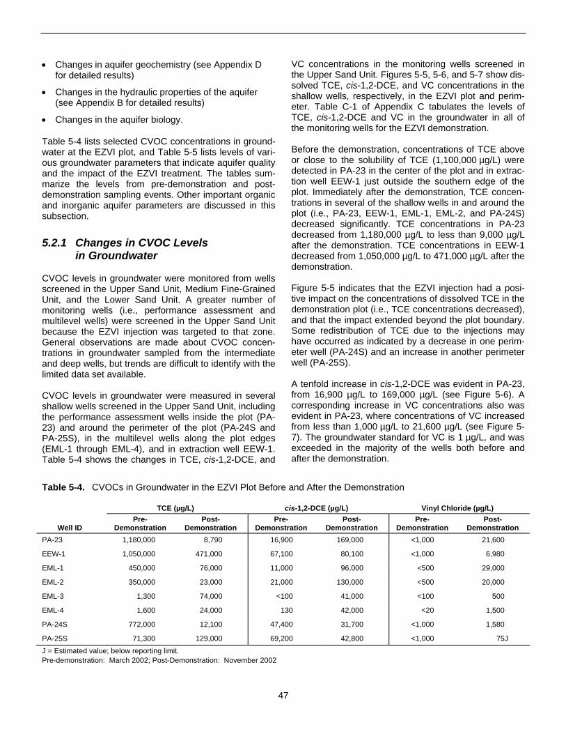
TCE (µg/L) cis-1,2-DCE (µg/L) Vinyl Chloride (µg/L)Pre- Post- Pre- Post- Pre- Post-

Well ID Demonstration Demonstration Demonstration Demonstration Demonstration Demonstration PA-23 1,180,000 8,790 16,900 169,000 <1,000 21,600

EEW-1 1,050,000 471,000 67,100 80,100 <1,000 6,980

EML-1 450,000 76,000 11,000 96,000 <500 29,000

EML-2 350,000 23,000 21,000 130,000 <500 20,000

EML-3 1,300 74,000 <100 41,000 <100 500

EML-4 1,600 24,000 130 42,000 <20 1,500

PA-24S 772,000 12,100 47,400 31,700 <1,000 1,580

PA-25S 71,300 129,000 69,200 42,800 <1,000 75J

J = Estimated value; below reporting limit. Pre-demonstration: March 2002; Post-Demonstration: November 2002

• Changes in aquifer geochemistry (see Appendix D for detailed results)

• Changes in the hydraulic properties of the aquifer (see Appendix B for detailed results)

• Changes in the aquifer biology.

Table 5-4 lists selected CVOC concentrations in ground­water at the EZVI plot, and Table 5-5 lists levels of vari­ous groundwater parameters that indicate aquifer quality and the impact of the EZVI treatment. The tables sum­marize the levels from pre-demonstration and post-demonstration sampling events. Other important organic and inorganic aquifer parameters are discussed in this subsection.

5.2.1 Changes in CVOC Levels in Groundwater

CVOC levels in groundwater were monitored from wells screened in the Upper Sand Unit, Medium Fine-Grained Unit, and the Lower Sand Unit. A greater number of monitoring wells (i.e., performance assessment and multilevel wells) were screened in the Upper Sand Unit because the EZVI injection was targeted to that zone. General observations are made about CVOC concen­trations in groundwater sampled from the intermediate and deep wells, but trends are difficult to identify with the limited data set available.

CVOC levels in groundwater were measured in several shallow wells screened in the Upper Sand Unit, including the performance assessment wells inside the plot (PA­23) and around the perimeter of the plot (PA-24S and PA-25S), in the multilevel wells along the plot edges (EML-1 through EML-4), and in extraction well EEW-1. Table 5-4 shows the changes in TCE, cis-1,2-DCE, and

VC concentrations in the monitoring wells screened in the Upper Sand Unit. Figures 5-5, 5-6, and 5-7 show dis­solved TCE, cis-1,2-DCE, and VC concentrations in the shallow wells, respectively, in the EZVI plot and perim­eter. Table C-1 of Appendix C tabulates the levels of TCE, cis-1,2-DCE and VC in the groundwater in all of the monitoring wells for the EZVI demonstration.

Before the demonstration, concentrations of TCE above or close to the solubility of TCE (1,100,000 µg/L) were detected in PA-23 in the center of the plot and in extrac­tion well EEW-1 just outside the southern edge of the plot. Immediately after the demonstration, TCE concen­trations in several of the shallow wells in and around the plot (i.e., PA-23, EEW-1, EML-1, EML-2, and PA-24S) decreased significantly. TCE concentrations in PA-23 decreased from 1,180,000 µg/L to less than 9,000 µg/L after the demonstration. TCE concentrations in EEW-1 decreased from 1,050,000 µg/L to 471,000 µg/L after the demonstration.

Figure 5-5 indicates that the EZVI injection had a posi­tive impact on the concentrations of dissolved TCE in the demonstration plot (i.e., TCE concentrations decreased), and that the impact extended beyond the plot boundary. Some redistribution of TCE due to the injections may have occurred as indicated by a decrease in one perim­eter well (PA-24S) and an increase in another perimeter well (PA-25S).

A tenfold increase in cis-1,2-DCE was evident in PA-23, from 16,900 µg/L to 169,000 µg/L (see Figure 5-6). A corresponding increase in VC concentrations also was evident in PA-23, where concentrations of VC increased from less than 1,000 µg/L to 21,600 µg/L (see Figure 5­7). The groundwater standard for VC is 1 µg/L, and was exceeded in the majority of the wells both before and after the demonstration.

Table 5-4. CVOCs in Groundwater in the EZVI Plot Before and After the Demonstration

47

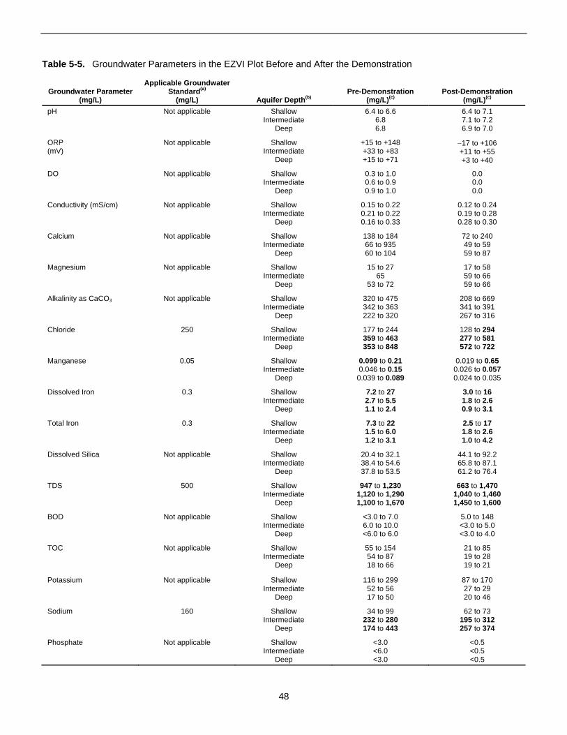
Table 5-5. Groundwater Parameters in the EZVI Plot Before and After the Demonstration

Groundwater Parameter Applicable Groundwater

Standard(a) Pre-Demonstration Post-Demonstration (mg/L) (mg/L) Aquifer Depth(b) (mg/L)(c) (mg/L)(c)

pH Not applicable Shallow 6.4 to 6.6 6.4 to 7.1 Intermediate 6.8 7.1 to 7.2

Deep 6.8 6.9 to 7.0

ORP Not applicable Shallow +15 to +148 −17 to +106 (mV) Intermediate +33 to +83 +11 to +55

Deep +15 to +71 +3 to +40

DO Not applicable Shallow 0.3 to 1.0 0.0 Intermediate 0.6 to 0.9 0.0

Deep 0.9 to 1.0 0.0

Conductivity (mS/cm) Not applicable Shallow 0.15 to 0.22 0.12 to 0.24 Intermediate 0.21 to 0.22 0.19 to 0.28

Deep 0.16 to 0.33 0.28 to 0.30

Calcium Not applicable Shallow 138 to 184 72 to 240 Intermediate 66 to 935 49 to 59

Deep 60 to 104 59 to 87

Magnesium Not applicable Shallow 15 to 27 17 to 58 Intermediate 65 59 to 66

Deep 53 to 72 59 to 66

Alkalinity as CaCO3 Not applicable Shallow 320 to 475 208 to 669 Intermediate 342 to 363 341 to 391

Deep 222 to 320 267 to 316

Chloride 250 Shallow 177 to 244 128 to 294 Intermediate 359 to 463 277 to 581

Deep 353 to 848 572 to 722

Manganese 0.05 Shallow 0.099 to 0.21 0.019 to 0.65 Intermediate 0.046 to 0.15 0.026 to 0.057

Deep 0.039 to 0.089 0.024 to 0.035

Dissolved Iron 0.3 Shallow 7.2 to 27 3.0 to 16 Intermediate 2.7 to 5.5 1.8 to 2.6

Deep 1.1 to 2.4 0.9 to 3.1

Total Iron 0.3 Shallow 7.3 to 22 2.5 to 17 Intermediate 1.5 to 6.0 1.8 to 2.6

Deep 1.2 to 3.1 1.0 to 4.2

Dissolved Silica Not applicable Shallow 20.4 to 32.1 44.1 to 92.2 Intermediate 38.4 to 54.6 65.8 to 87.1

Deep 37.8 to 53.5 61.2 to 76.4

TDS 500 Shallow 947 to 1,230 663 to 1,470 Intermediate 1,120 to 1,290 1,040 to 1,460

Deep 1,100 to 1,670 1,450 to 1,600

BOD Not applicable Shallow <3.0 to 7.0 5.0 to 148 Intermediate 6.0 to 10.0 <3.0 to 5.0

Deep <6.0 to 6.0 <3.0 to 4.0

TOC Not applicable Shallow 55 to 154 21 to 85 Intermediate 54 to 87 19 to 28

Deep 18 to 66 19 to 21

Potassium Not applicable Shallow 116 to 299 87 to 170 Intermediate 52 to 56 27 to 29

Deep 17 to 50 20 to 46

Sodium 160 Shallow 34 to 99 62 to 73 Intermediate 232 to 280 195 to 312

Deep 174 to 443 257 to 374

Phosphate Not applicable Shallow <3.0 <0.5 Intermediate <6.0 <0.5

Deep <3.0 <0.5

48

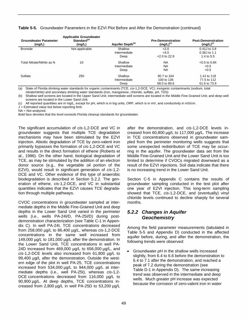
Table 5-5. Groundwater Parameters in the EZVI Plot Before and After the Demonstration (continued)

Groundwater Parameter (mg/L)

Bromide

Applicable Groundwater Standard(a)

(mg/L) Not applicable

Aquifer Depth(b)

Shallow Intermediate

Pre-Demonstration (mg/L)(c)

<2.0 <4.0

Post-Demonstration (mg/L)(c)

0.41J to 3.8 0.36J to 1.1

Deep <2.0 to 22.9 1.4 to 5.5

Total Nitrate/Nitrite as N 10 Shallow Intermediate

NA NA

<0.5 to 0.84 <0.5

Deep NA <0.5

Sulfate 250 Shallow 90.7 to 164 1.4J to 118 Intermediate 100 to 136 77.5 to 112

Deep 58.0 to 89.6 61.6 to 73.9 (a) State of Florida drinking water standards for organic contaminants (TCE, cis-1,2-DCE, VC), inorganic contaminants (sodium, total

nitrate/nitrite) and secondary drinking water standards (iron, manganese, chloride, sulfate, pH, TDS) (b) Shallow well screens are located in the Upper Sand Unit; intermediate well screens are located in the Middle Fine-Grained Unit; and deep well

screens are located in the Lower Sand Unit. (c) All reported quantities are in mg/L, except for pH, which is in log units, ORP, which is in mV, and conductivity in mS/cm. J = Estimated value but below reporting limit. NA = Not analyzed. Bold face denotes that the level exceeds Florida cleanup standards for groundwater.

The significant accumulation of cis-1,2-DCE and VC in groundwater suggests that multiple TCE degradation mechanisms may have been stimulated by the EZVI injection. Abiotic degradation of TCE by zero-valent iron primarily bypasses the formation of cis-1,2-DCE and VC and results in the direct formation of ethene (Roberts et al., 1996). On the other hand, biological degradation of TCE, as may be stimulated by the addition of an electron donor source (e.g., the vegetable oil portion of the EZVI), would result in significant generation of cis-1,2­DCE and VC. Other evidence of this type of anaerobic biodegradation is described in Section 5.2.2. The gen­eration of ethene, cis-1,2-DCE, and VC in substantial quantities indicates that the EZVI causes TCE degrada­tion through multiple pathways.

CVOC concentrations in groundwater sampled at inter­mediate depths in the Middle Fine-Grained Unit and deep depths in the Lower Sand Unit varied in the perimeter wells (i.e., wells PA-24I/D, PA-25I/D) during post-demonstration characterization (see Table C-1 in Appen­dix C). In well PA-24I, TCE concentrations decreased from 258,000 µg/L to 86,400 µg/L, whereas cis-1,2-DCE concentrations in the same well increased from 149,000 µg/L to 181,000 µg/L after the demonstration. In the Lower Sand Unit, TCE concentrations in well PA­24D increased from 469,000 µg/L to 656,000 µg/L, and cis-1,2-DCE levels also increased from 61,800 µg/L to 99,400 µg/L after the demonstration. Outside the west­ern edge of the plot in well PA-25, TCE concentrations increased from 534,000 µg/L to 944,000 µg/L at inter­mediate depths (i.e., well PA-25I), whereas cis-1,2­DCE concentrations decreased from 116,000 µg/L to 90,900 µg/L. At deep depths, TCE concentrations in­creased from 2,800 µg/L in well PA-25D to 53,200 µg/L

after the demonstration, and cis-1,2-DCE levels in­creased from 60,800 µg/L to 117,000 µg/L. The increase in TCE concentrations observed in groundwater sam­pled from the perimeter monitoring wells suggests that some unexpected redistribution of TCE may be occur­ring in the aquifer. The groundwater data set from the Middle Fine-Grained Unit and the Lower Sand Unit is too limited to determine if CVOCs migrated downward as a result of the EZVI injections. Soil data indicate that there is no increasing trend in the Lower Sand Unit.

Section C-5 in Appendix C contains the results of groundwater sampling conducted in the test plot after one year of EZVI injection. This long-term sampling showed that TCE, cis-1,2-DCE, and (eventually) vinyl chloride levels continued to decline sharply for several months.

5.2.2 Changes in Aquifer Geochemistry

Among the field parameter measurements (tabulated in Table 5-5 and Appendix D) conducted in the affected aquifer before, during, and after the demonstration, the following trends were observed:

• Groundwater pH in the shallow wells increased slightly, from 6.4 to 6.6 before the demonstration to 6.4 to 7.1 after the demonstration, and reached a peak of 7.2 during the demonstration (see Table D-1 in Appendix D). The same increasing trend was observed in the intermediate and deep wells. Much greater pH increase was expected because the corrosion of zero-valent iron in water

49

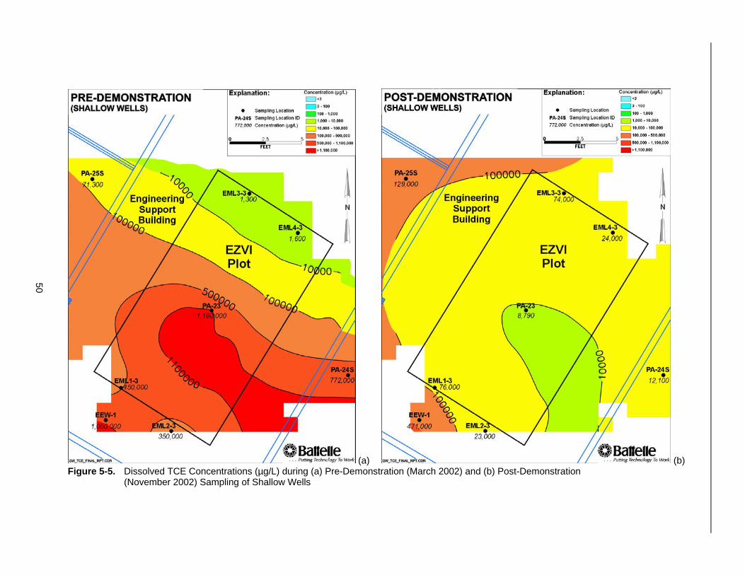
50

(a) (b) Figure 5-5. Dissolved TCE Concentrations (µg/L) during (a) Pre-Demonstration (March 2002) and (b) Post-Demonstration

(November 2002) Sampling of Shallow Wells

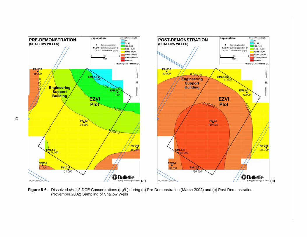
51

(a) (b)

Figure 5-6. Dissolved cis-1,2-DCE Concentrations (µg/L) during (a) Pre-Demonstration (March 2002) and (b) Post-Demonstration (November 2002) Sampling of Shallow Wells

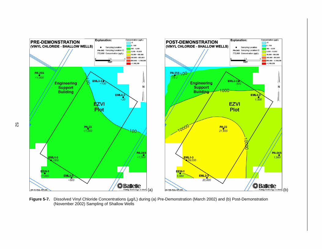
52

(a) (b)

Figure 5-7. Dissolved Vinyl Chloride Concentrations (µg/L) during (a) Pre-Demonstration (March 2002) and (b) Post-Demonstration (November 2002) Sampling of Shallow Wells

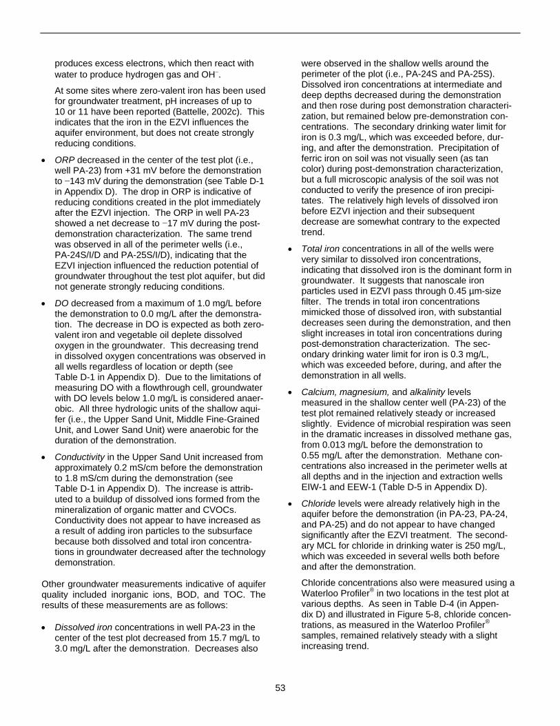
produces excess electrons, which then react with water to produce hydrogen gas and OH− .

At some sites where zero-valent iron has been used for groundwater treatment, pH increases of up to 10 or 11 have been reported (Battelle, 2002c). This indicates that the iron in the EZVI influences the aquifer environment, but does not create strongly reducing conditions.

• ORP decreased in the center of the test plot (i.e., well PA-23) from +31 mV before the demonstration to −143 mV during the demonstration (see Table D-1 in Appendix D). The drop in ORP is indicative of reducing conditions created in the plot immediately after the EZVI injection. The ORP in well PA-23 showed a net decrease to −17 mV during the post-demonstration characterization. The same trend was observed in all of the perimeter wells (i.e., PA-24S/I/D and PA-25S/I/D), indicating that the EZVI injection influenced the reduction potential of groundwater throughout the test plot aquifer, but did not generate strongly reducing conditions.

• DO decreased from a maximum of 1.0 mg/L before the demonstration to 0.0 mg/L after the demonstra­tion. The decrease in DO is expected as both zero-valent iron and vegetable oil deplete dissolved oxygen in the groundwater. This decreasing trend in dissolved oxygen concentrations was observed in all wells regardless of location or depth (see Table D-1 in Appendix D). Due to the limitations of measuring DO with a flowthrough cell, groundwater with DO levels below 1.0 mg/L is considered anaer­obic. All three hydrologic units of the shallow aqui­fer (i.e., the Upper Sand Unit, Middle Fine-Grained Unit, and Lower Sand Unit) were anaerobic for the duration of the demonstration.

• Conductivity in the Upper Sand Unit increased from approximately 0.2 mS/cm before the demonstration to 1.8 mS/cm during the demonstration (see Table D-1 in Appendix D). The increase is attrib­uted to a buildup of dissolved ions formed from the mineralization of organic matter and CVOCs. Conductivity does not appear to have increased as a result of adding iron particles to the subsurface because both dissolved and total iron concentra­tions in groundwater decreased after the technology demonstration.

Other groundwater measurements indicative of aquifer quality included inorganic ions, BOD, and TOC. The results of these measurements are as follows:

• Dissolved iron concentrations in well PA-23 in the center of the test plot decreased from 15.7 mg/L to 3.0 mg/L after the demonstration. Decreases also

were observed in the shallow wells around the perimeter of the plot (i.e., PA-24S and PA-25S). Dissolved iron concentrations at intermediate and deep depths decreased during the demonstration and then rose during post demonstration characteri­zation, but remained below pre-demonstration con­centrations. The secondary drinking water limit for iron is 0.3 mg/L, which was exceeded before, dur­ing, and after the demonstration. Precipitation of ferric iron on soil was not visually seen (as tan color) during post-demonstration characterization, but a full microscopic analysis of the soil was not conducted to verify the presence of iron precipi­tates. The relatively high levels of dissolved iron before EZVI injection and their subsequent decrease are somewhat contrary to the expected trend.

• Total iron concentrations in all of the wells were very similar to dissolved iron concentrations, indicating that dissolved iron is the dominant form in groundwater. It suggests that nanoscale iron particles used in EZVI pass through 0.45 µm-size filter. The trends in total iron concentrations mimicked those of dissolved iron, with substantial decreases seen during the demonstration, and then slight increases in total iron concentrations during post-demonstration characterization. The sec­ondary drinking water limit for iron is 0.3 mg/L, which was exceeded before, during, and after the demonstration in all wells.

• Calcium, magnesium, and alkalinity levels measured in the shallow center well (PA-23) of the test plot remained relatively steady or increased slightly. Evidence of microbial respiration was seen in the dramatic increases in dissolved methane gas, from 0.013 mg/L before the demonstration to 0.55 mg/L after the demonstration. Methane con­centrations also increased in the perimeter wells at all depths and in the injection and extraction wells EIW-1 and EEW-1 (Table D-5 in Appendix D).

• Chloride levels were already relatively high in the aquifer before the demonstration (in PA-23, PA-24, and PA-25) and do not appear to have changed significantly after the EZVI treatment. The second­ary MCL for chloride in drinking water is 250 mg/L, which was exceeded in several wells both before and after the demonstration.

Chloride concentrations also were measured using a Waterloo Profiler® in two locations in the test plot at various depths. As seen in Table D-4 (in Appen­dix D) and illustrated in Figure 5-8, chloride concen­trations, as measured in the Waterloo Profiler®

samples, remained relatively steady with a slight increasing trend.

53

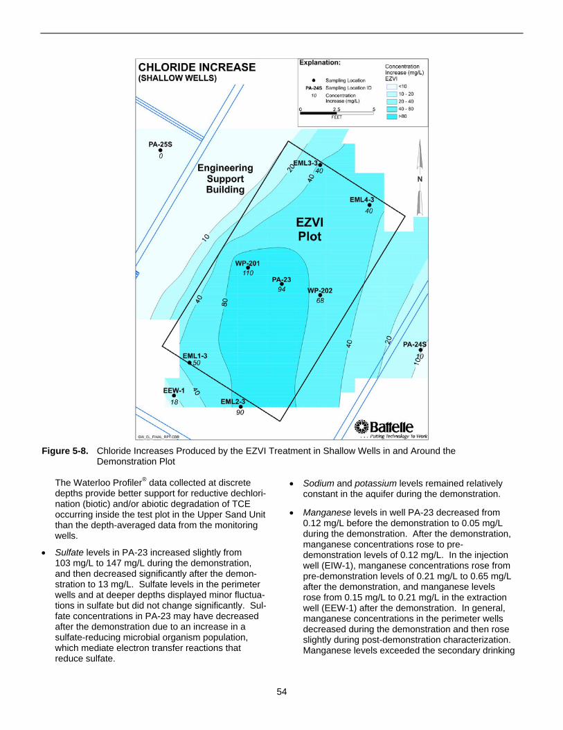
Figure 5-8. Chloride Increases Produced by the EZVI Treatment in Shallow Wells in and Around the Demonstration Plot

The Waterloo Profiler® data collected at discrete depths provide better support for reductive dechlori­nation (biotic) and/or abiotic degradation of TCE occurring inside the test plot in the Upper Sand Unit than the depth-averaged data from the monitoring wells.

• Sulfate levels in PA-23 increased slightly from 103 mg/L to 147 mg/L during the demonstration, and then decreased significantly after the demon­stration to 13 mg/L. Sulfate levels in the perimeter wells and at deeper depths displayed minor fluctua­tions in sulfate but did not change significantly. Sul­fate concentrations in PA-23 may have decreased after the demonstration due to an increase in a sulfate-reducing microbial organism population, which mediate electron transfer reactions that reduce sulfate.

• Sodium and potassium levels remained relatively constant in the aquifer during the demonstration.

• Manganese levels in well PA-23 decreased from 0.12 mg/L before the demonstration to 0.05 mg/L during the demonstration. After the demonstration, manganese concentrations rose to pre-demonstration levels of 0.12 mg/L. In the injection well (EIW-1), manganese concentrations rose from pre-demonstration levels of 0.21 mg/L to 0.65 mg/L after the demonstration, and manganese levels rose from 0.15 mg/L to 0.21 mg/L in the extraction well (EEW-1) after the demonstration. In general, manganese concentrations in the perimeter wells decreased during the demonstration and then rose slightly during post-demonstration characterization. Manganese levels exceeded the secondary drinking

54

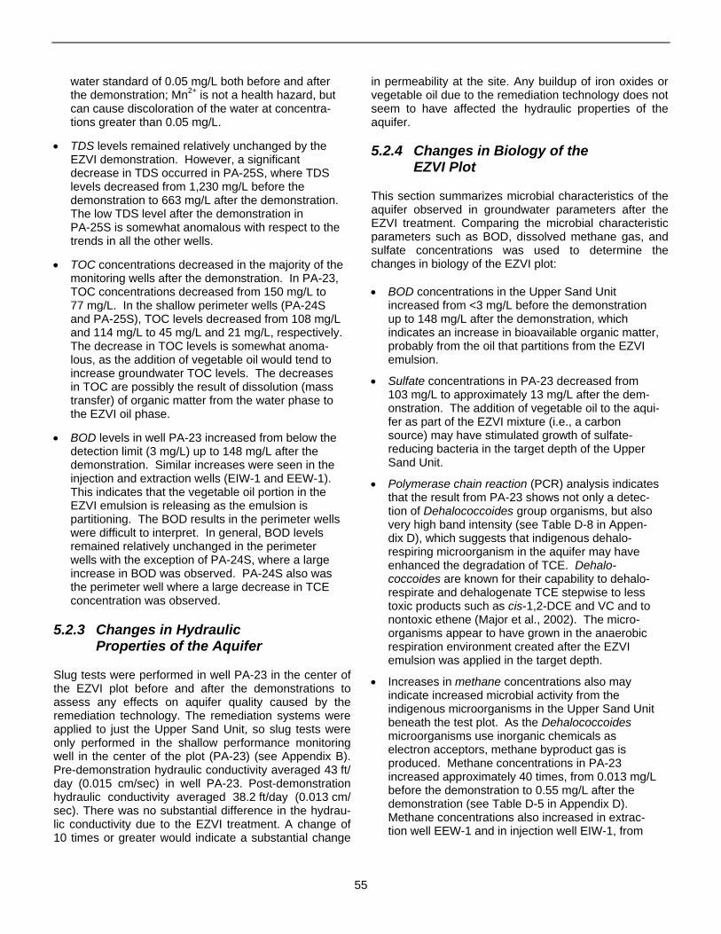
water standard of 0.05 mg/L both before and after the demonstration; Mn2+ is not a health hazard, but can cause discoloration of the water at concentra­tions greater than 0.05 mg/L.

• TDS levels remained relatively unchanged by the EZVI demonstration. However, a significant decrease in TDS occurred in PA-25S, where TDS levels decreased from 1,230 mg/L before the demonstration to 663 mg/L after the demonstration. The low TDS level after the demonstration in PA-25S is somewhat anomalous with respect to the trends in all the other wells.

• TOC concentrations decreased in the majority of the monitoring wells after the demonstration. In PA-23, TOC concentrations decreased from 150 mg/L to 77 mg/L. In the shallow perimeter wells (PA-24S and PA-25S), TOC levels decreased from 108 mg/L and 114 mg/L to 45 mg/L and 21 mg/L, respectively. The decrease in TOC levels is somewhat anoma­lous, as the addition of vegetable oil would tend to increase groundwater TOC levels. The decreases in TOC are possibly the result of dissolution (mass transfer) of organic matter from the water phase to the EZVI oil phase.

• BOD levels in well PA-23 increased from below the detection limit (3 mg/L) up to 148 mg/L after the demonstration. Similar increases were seen in the injection and extraction wells (EIW-1 and EEW-1). This indicates that the vegetable oil portion in the EZVI emulsion is releasing as the emulsion is partitioning. The BOD results in the perimeter wells were difficult to interpret. In general, BOD levels remained relatively unchanged in the perimeter wells with the exception of PA-24S, where a large increase in BOD was observed. PA-24S also was the perimeter well where a large decrease in TCE concentration was observed.

5.2.3 Changes in Hydraulic Properties of the Aquifer

Slug tests were performed in well PA-23 in the center of the EZVI plot before and after the demonstrations to assess any effects on aquifer quality caused by the remediation technology. The remediation systems were applied to just the Upper Sand Unit, so slug tests were only performed in the shallow performance monitoring well in the center of the plot (PA-23) (see Appendix B). Pre-demonstration hydraulic conductivity averaged 43 ft/ day (0.015 cm/sec) in well PA-23. Post-demonstration hydraulic conductivity averaged 38.2 ft/day (0.013 cm/ sec). There was no substantial difference in the hydrau­lic conductivity due to the EZVI treatment. A change of 10 times or greater would indicate a substantial change

in permeability at the site. Any buildup of iron oxides or vegetable oil due to the remediation technology does not seem to have affected the hydraulic properties of the aquifer.

5.2.4 Changes in Biology of the EZVI Plot

This section summarizes microbial characteristics of the aquifer observed in groundwater parameters after the EZVI treatment. Comparing the microbial characteristic parameters such as BOD, dissolved methane gas, and sulfate concentrations was used to determine the changes in biology of the EZVI plot:

• BOD concentrations in the Upper Sand Unit increased from <3 mg/L before the demonstration up to 148 mg/L after the demonstration, which indicates an increase in bioavailable organic matter, probably from the oil that partitions from the EZVI emulsion.

• Sulfate concentrations in PA-23 decreased from 103 mg/L to approximately 13 mg/L after the dem­onstration. The addition of vegetable oil to the aqui­fer as part of the EZVI mixture (i.e., a carbon source) may have stimulated growth of sulfate-reducing bacteria in the target depth of the Upper Sand Unit.

• Polymerase chain reaction (PCR) analysis indicates that the result from PA-23 shows not only a detec­tion of Dehalococcoides group organisms, but also very high band intensity (see Table D-8 in Appen­dix D), which suggests that indigenous dehalo­respiring microorganism in the aquifer may have enhanced the degradation of TCE. Dehalo-coccoides are known for their capability to dehalo­respirate and dehalogenate TCE stepwise to less toxic products such as cis-1,2-DCE and VC and to nontoxic ethene (Major et al., 2002). The micro­organisms appear to have grown in the anaerobic respiration environment created after the EZVI emulsion was applied in the target depth.

• Increases in methane concentrations also may indicate increased microbial activity from the indigenous microorganisms in the Upper Sand Unit beneath the test plot. As the Dehalococcoides microorganisms use inorganic chemicals as electron acceptors, methane byproduct gas is produced. Methane concentrations in PA-23 increased approximately 40 times, from 0.013 mg/L before the demonstration to 0.55 mg/L after the demonstration (see Table D-5 in Appendix D). Methane concentrations also increased in extrac­tion well EEW-1 and in injection well EIW-1, from

55

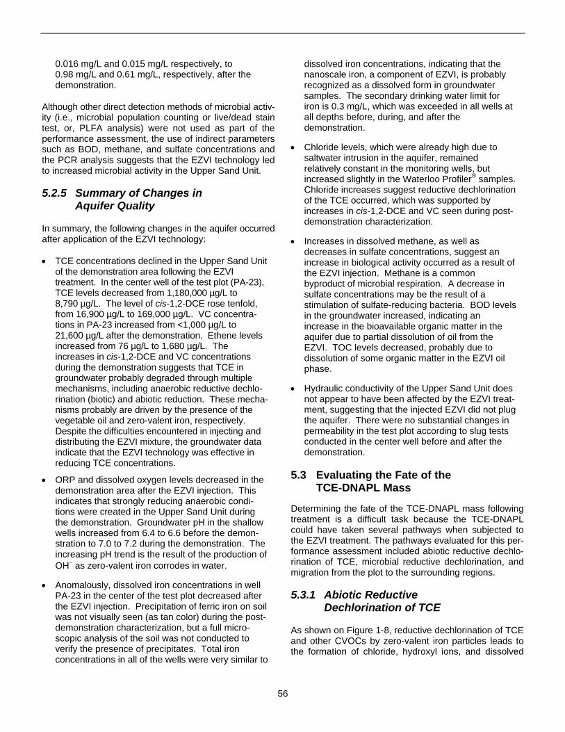
0.016 mg/L and 0.015 mg/L respectively, to 0.98 mg/L and 0.61 mg/L, respectively, after the demonstration.

Although other direct detection methods of microbial activ­ity (i.e., microbial population counting or live/dead stain test, or, PLFA analysis) were not used as part of the performance assessment, the use of indirect parameters such as BOD, methane, and sulfate concentrations and the PCR analysis suggests that the EZVI technology led to increased microbial activity in the Upper Sand Unit.

5.2.5 Summary of Changes in Aquifer Quality

In summary, the following changes in the aquifer occurred after application of the EZVI technology:

• TCE concentrations declined in the Upper Sand Unit of the demonstration area following the EZVI treatment. In the center well of the test plot (PA-23), TCE levels decreased from 1,180,000 µg/L to 8,790 µg/L. The level of cis-1,2-DCE rose tenfold, from 16,900 µg/L to 169,000 µg/L. VC concentra­tions in PA-23 increased from <1,000 µg/L to 21,600 µg/L after the demonstration. Ethene levels increased from 76 µg/L to 1,680 µg/L. The increases in cis-1,2-DCE and VC concentrations during the demonstration suggests that TCE in groundwater probably degraded through multiple mechanisms, including anaerobic reductive dechlo­rination (biotic) and abiotic reduction. These mecha­nisms probably are driven by the presence of the vegetable oil and zero-valent iron, respectively. Despite the difficulties encountered in injecting and distributing the EZVI mixture, the groundwater data indicate that the EZVI technology was effective in reducing TCE concentrations.

• ORP and dissolved oxygen levels decreased in the demonstration area after the EZVI injection. This indicates that strongly reducing anaerobic condi­tions were created in the Upper Sand Unit during the demonstration. Groundwater pH in the shallow wells increased from 6.4 to 6.6 before the demon­stration to 7.0 to 7.2 during the demonstration. The increasing pH trend is the result of the production of OH− as zero-valent iron corrodes in water.

• Anomalously, dissolved iron concentrations in well PA-23 in the center of the test plot decreased after the EZVI injection. Precipitation of ferric iron on soil was not visually seen (as tan color) during the post-demonstration characterization, but a full micro­scopic analysis of the soil was not conducted to verify the presence of precipitates. Total iron concentrations in all of the wells were very similar to

dissolved iron concentrations, indicating that the nanoscale iron, a component of EZVI, is probably recognized as a dissolved form in groundwater samples. The secondary drinking water limit for iron is 0.3 mg/L, which was exceeded in all wells at all depths before, during, and after the demonstration.

• Chloride levels, which were already high due to saltwater intrusion in the aquifer, remained relatively constant in the monitoring wells, but increased slightly in the Waterloo Profiler® samples. Chloride increases suggest reductive dechlorination of the TCE occurred, which was supported by increases in cis-1,2-DCE and VC seen during post-demonstration characterization.

• Increases in dissolved methane, as well as decreases in sulfate concentrations, suggest an increase in biological activity occurred as a result of the EZVI injection. Methane is a common byproduct of microbial respiration. A decrease in sulfate concentrations may be the result of a stimulation of sulfate-reducing bacteria. BOD levels in the groundwater increased, indicating an increase in the bioavailable organic matter in the aquifer due to partial dissolution of oil from the EZVI. TOC levels decreased, probably due to dissolution of some organic matter in the EZVI oil phase.

• Hydraulic conductivity of the Upper Sand Unit does not appear to have been affected by the EZVI treat­ment, suggesting that the injected EZVI did not plug the aquifer. There were no substantial changes in permeability in the test plot according to slug tests conducted in the center well before and after the demonstration.

5.3 Evaluating the Fate of the TCE-DNAPL Mass

Determining the fate of the TCE-DNAPL mass following treatment is a difficult task because the TCE-DNAPL could have taken several pathways when subjected to the EZVI treatment. The pathways evaluated for this per­formance assessment included abiotic reductive dechlo­rination of TCE, microbial reductive dechlorination, and migration from the plot to the surrounding regions.

5.3.1 Abiotic Reductive Dechlorination of TCE

As shown on Figure 1-8, reductive dechlorination of TCE and other CVOCs by zero-valent iron particles leads to the formation of chloride, hydroxyl ions, and dissolved

56

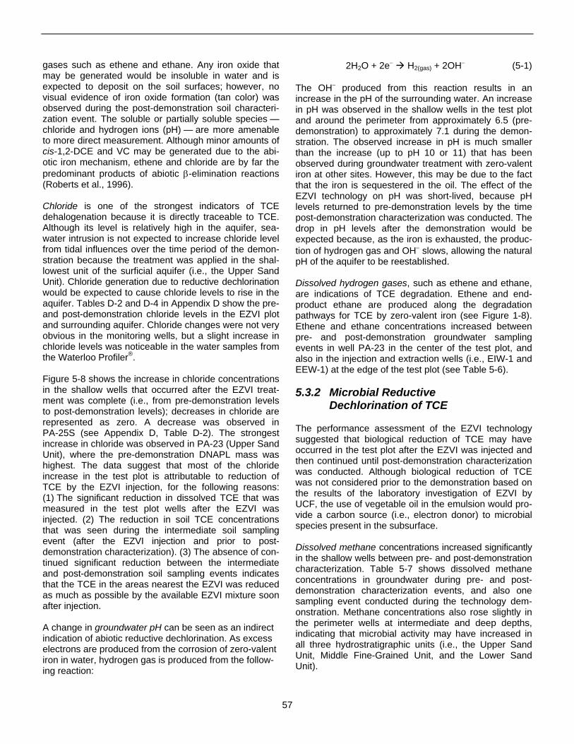
gases such as ethene and ethane. Any iron oxide that may be generated would be insoluble in water and is expected to deposit on the soil surfaces; however, no visual evidence of iron oxide formation (tan color) was observed during the post-demonstration soil characteri­zation event. The soluble or partially soluble species — chloride and hydrogen ions (pH) — are more amenable to more direct measurement. Although minor amounts of cis-1,2-DCE and VC may be generated due to the abi­otic iron mechanism, ethene and chloride are by far the predominant products of abiotic β-elimination reactions (Roberts et al., 1996).

Chloride is one of the strongest indicators of TCE dehalogenation because it is directly traceable to TCE. Although its level is relatively high in the aquifer, sea­water intrusion is not expected to increase chloride level from tidal influences over the time period of the demon­stration because the treatment was applied in the shal­lowest unit of the surficial aquifer (i.e., the Upper Sand Unit). Chloride generation due to reductive dechlorination would be expected to cause chloride levels to rise in the aquifer. Tables D-2 and D-4 in Appendix D show the pre- and post-demonstration chloride levels in the EZVI plot and surrounding aquifer. Chloride changes were not very obvious in the monitoring wells, but a slight increase in chloride levels was noticeable in the water samples from the Waterloo Profiler®.

Figure 5-8 shows the increase in chloride concentrations in the shallow wells that occurred after the EZVI treat­ment was complete (i.e., from pre-demonstration levels to post-demonstration levels); decreases in chloride are represented as zero. A decrease was observed in PA-25S (see Appendix D, Table D-2). The strongest increase in chloride was observed in PA-23 (Upper Sand Unit), where the pre-demonstration DNAPL mass was highest. The data suggest that most of the chloride increase in the test plot is attributable to reduction of TCE by the EZVI injection, for the following reasons: (1) The significant reduction in dissolved TCE that was measured in the test plot wells after the EZVI was injected. (2) The reduction in soil TCE concentrations that was seen during the intermediate soil sampling event (after the EZVI injection and prior to post-demonstration characterization). (3) The absence of con­tinued significant reduction between the intermediate and post-demonstration soil sampling events indicates that the TCE in the areas nearest the EZVI was reduced as much as possible by the available EZVI mixture soon after injection.

A change in groundwater pH can be seen as an indirect indication of abiotic reductive dechlorination. As excess electrons are produced from the corrosion of zero-valent iron in water, hydrogen gas is produced from the follow­ing reaction:

2H2O + 2e− Æ H2(gas) + 2OH− (5-1)

The OH− produced from this reaction results in an increase in the pH of the surrounding water. An increase in pH was observed in the shallow wells in the test plot and around the perimeter from approximately 6.5 (pre­demonstration) to approximately 7.1 during the demon­stration. The observed increase in pH is much smaller than the increase (up to pH 10 or 11) that has been observed during groundwater treatment with zero-valent iron at other sites. However, this may be due to the fact that the iron is sequestered in the oil. The effect of the EZVI technology on pH was short-lived, because pH levels returned to pre-demonstration levels by the time post-demonstration characterization was conducted. The drop in pH levels after the demonstration would be expected because, as the iron is exhausted, the produc­tion of hydrogen gas and OH− slows, allowing the natural pH of the aquifer to be reestablished.

Dissolved hydrogen gases, such as ethene and ethane, are indications of TCE degradation. Ethene and end-product ethane are produced along the degradation pathways for TCE by zero-valent iron (see Figure 1-8). Ethene and ethane concentrations increased between pre- and post-demonstration groundwater sampling events in well PA-23 in the center of the test plot, and also in the injection and extraction wells (i.e., EIW-1 and EEW-1) at the edge of the test plot (see Table 5-6).

5.3.2 Microbial Reductive Dechlorination of TCE

The performance assessment of the EZVI technology suggested that biological reduction of TCE may have occurred in the test plot after the EZVI was injected and then continued until post-demonstration characterization was conducted. Although biological reduction of TCE was not considered prior to the demonstration based on the results of the laboratory investigation of EZVI by UCF, the use of vegetable oil in the emulsion would pro­vide a carbon source (i.e., electron donor) to microbial species present in the subsurface.

Dissolved methane concentrations increased significantly in the shallow wells between pre- and post-demonstration characterization. Table 5-7 shows dissolved methane concentrations in groundwater during pre- and post-demonstration characterization events, and also one sampling event conducted during the technology dem­onstration. Methane concentrations also rose slightly in the perimeter wells at intermediate and deep depths, indicating that microbial activity may have increased in all three hydrostratigraphic units (i.e., the Upper Sand Unit, Middle Fine-Grained Unit, and the Lower Sand Unit).

57

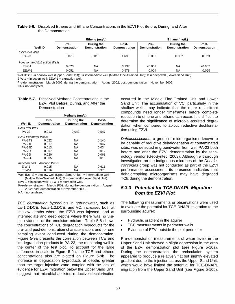
Well ID

Ethene (mg/L) Ethane (mg/L) Pre-

Demonstration During the

Demonstration Post-

Demonstration Pre-

Demonstration During the

Demonstration Post-

Demonstration EZVI Plot Well

PA-23 0.076 0.010 1.68 0.002 0.002 0.023

Injection and Extraction Wells EIW-1 0.023 NA 0.137 <0.002 NA <0.002 EEW-1 0.051 NA 0.978 0.004 NA 0.055

Well ID

Methane (mg/L)Pre-

Demonstration During the

Demonstration Post-

Demonstration EZVI Plot Well

PA-23 0.013 0.043 0.547 EZVI Perimeter Wells

PA-24S 0.022 NA 0.140 PA-24I 0.017 NA 0.047 PA-24D 0.013 NA 0.034 PA-25S 0.007 NA 0.012 PA-25I 0.020 NA 0.061 PA-25D 0.005 NA 0.016

Injection and Extraction Wells EIW-1 0.015 NA 0.611 EEW-1 0.016 NA 0.978

Table 5-6. Dissolved Ethene and Ethane Concentrations in the EZVI Plot Before, During, and After the Demonstration

Well IDs: S = shallow well (Upper Sand Unit); I = intermediate well (Middle Fine-Grained Unit); D = deep well (Lower Sand Unit). EIW-1 = injection well; EEW-1 = extraction well. Pre-demonstration = March 2002; during the demonstration = August 2002; post-demonstration = November 2002. NA = not analyzed.

Table 5-7. Dissolved Methane Concentrations in the EZVI Plot Before, During, and After the Demonstration

Well IDs: S = shallow well (Upper Sand Unit); I = intermediate well (Middle Fine-Grained Unit); D = deep well (Lower Sand Unit).

EIW-1 = injection well; EEW-1 = extraction well. Pre-demonstration = March 2002; during the demonstration = August

2002; post-demonstration = November 2002. NA = not analyzed.

TCE degradation byproducts in groundwater, such as cis-1,2-DCE, trans-1,2,DCE, and VC, increased both at shallow depths where the EZVI was injected, and at intermediate and deep depths where there was no visi­ble evidence of the emulsion mixture. Table 5-8 shows the concentrations of TCE degradation byproducts for the pre- and post-demonstration characterization, and for one sampling event conducted during the demonstration. Figure 5-9a presents the correlation between TCE and its degradation products in PA-23, the monitoring well in the center of the test plot. To account for the large difference in scale in Figure 5-9a, the TCE and ethene concentrations also are plotted on Figure 5-9b. The increase in degradation byproducts at depths greater than the target injection zone, coupled with the lack of evidence for EZVI migration below the Upper Sand Unit, suggest that microbial-assisted reductive dechlorination

occurred in the Middle Fine-Grained Unit and Lower Sand Unit. The accumulation of VC, particularly in the shallow wells, may indicate that the more recalcitrant compounds need longer timeframes before complete reduction to ethene and ethane can occur. It is difficult to determine the significance of microbial-assisted degra­dation when compared to abiotic reductive dechlorina­tion using EZVI.

Dehalococcoides, a group of microorganisms known to be capable of reductive dehalogenation at contaminated sites, was detected in groundwater from well PA-23 both before and after the EZVI demonstration by the tech­nology vendor (GeoSyntec, 2003). Although a thorough investigation on the indigenous microbes of the Dehalo-coccoides group was not conducted as part of the EZVI performance assessment, its presence indicates that dehalorespiring microorganisms may have degraded TCE during the demonstration.

5.3.3 Potential for TCE-DNAPL Migration from the EZVI Plot

The following measurements or observations were used to evaluate the potential for TCE-DNAPL migration to the surrounding aquifer:

• Hydraulic gradient in the aquifer • TCE measurements in perimeter wells • Evidence of EZVI outside the plot perimeter

Pre-demonstration measurements of water levels in the Upper Sand Unit showed a slight depression in the area of the EZVI demonstration plot (see Figure 5-10a). During the demonstration, the recirculation system appeared to produce a relatively flat but slightly elevated gradient due to the injection across the Upper Sand Unit, which would have limited the potential for TCE-DNAPL migration from the Upper Sand Unit (see Figure 5-10b).

58

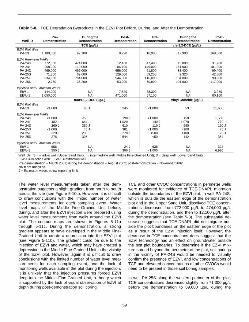
Well ID Pre-

Demonstration During the

Demonstration Post-

Demonstration Pre-

Demonstration During the

Demonstration Post-

Demonstration TCE (µg/L) cis-1,2-DCE (µg/L)

EZVI Plot Well PA-23 1,180,000 92,100 8,790 16,900 17,900 169,000

EZVI Perimeter Wells PA-24S 772,000 474,000 12,100 47,400 15,800 31,700 PA-24I 258,000 110,000 86,400 149,000 161,000 181,000 PA-24D 469,000 497,000 656,000 61,800 83,400 99,400 PA-25S 71,300 69,600 129,000 69,200 9,320 42,800 PA-25I 534,000 784,000 944,000 116,000 104,000 90,900 PA-25D 2,760 36,200 53,200 60,800 101,000 117,000

Injection and Extraction Wells EIW-1 144,000 NA 7,820 38,300 NA 3,280 EEW-1 1,050,000 NA 471,000 67,100 NA 80,100

trans-1,2-DCE (µg/L) Vinyl Chloride (µg/L) EZVI Plot Well

PA-23 <1,000 68 J 245 <1,000 53 J 21,600

EZVI Perimeter Wells PA-24S <1,000 <50 190 J <1,000 <50 1,580 PA-24I 482 644 1,020 140 J 1,070 779 PA-24D 260 J 360 J 610 110 J 590 160 J PA-25S <1,000 46 J 381 <1,000 <100 75 J PA-25I 320 J 230 270 J <500 <100 170 J PA-25D 278 395 544 <50 142 354

Injection and Extraction Wells EIW-1 556 NA 24 J 638 NA 322 EEW-1 550 J NA 390 J <1,000 NA 6,980

Table 5-8. TCE Degradation Byproducts in the EZVI Plot Before, During, and After the Demonstration

Well IDs: S = shallow well (Upper Sand Unit); I = intermediate well (Middle Fine-Grained Unit); D = deep well (Lower Sand Unit). EIW-1 = injection well; EEW-1 = extraction well. Pre-demonstration = March 2002; during the demonstration = August 2002; post-demonstration = November 2002 NA = not analyzed. J = Estimated value, below reporting limit.

The water level measurements taken after the dem­onstration suggests a slight gradient from north to south across the site (see Figure 5-10c). However, it is difficult to draw conclusions with the limited number of water level measurements for each sampling event. Water level maps of the Middle Fine-Grained Unit before, during, and after the EZVI injection were prepared using water level measurements from wells around the EZVI plot. The contour maps are shown in Figures 5-11a through 5-11c. During the demonstration, a strong gradient appears to have developed in the Middle Fine-Grained Unit to create a depression into the EZVI plot (see Figure 5-11b). The gradient could be due to the injection of EZVI and water, which may have created a depression in the Middle Fine-Grained Unit in the vicinity of the EZVI plot. However, again it is difficult to draw conclusions with the limited number of water level mea­surements for each sampling event, and the lack of monitoring wells available in the plot during the injection. It is unlikely that the injection pressures forced EZVI deep into the Middle Fine-Grained Unit, a theory which is supported by the lack of visual observation of EZVI at depth during post-demonstration soil coring.

TCE and other CVOC concentrations in perimeter wells were monitored for evidence of TCE-DNAPL migration outside the boundaries of the EZVI plot. In well PA-24S, which is outside the eastern edge of the demonstration plot and in the Upper Sand Unit, dissolved TCE concen­trations decreased from 772,000 µg/L to 474,000 µg/L during the demonstration, and then to 12,100 µg/L after the demonstration (see Table 5-8). The substantial de­crease suggests that TCE-DNAPL did not migrate out­side the plot boundaries on the eastern edge of the plot as a result of the EZVI injection itself. However, the decrease in TCE concentrations does suggest that the EZVI technology had an effect on groundwater outside the test plot boundaries. To determine if the EZVI mix­ture spread beyond the perimeter of the plot, soil borings in the vicinity of PA-24S would be needed to visually confirm the presence of EZVI, and low concentrations of TCE and elevated concentrations of other CVOCs would need to be present in those soil boring samples.

In well PA-25S along the western perimeter of the plot, TCE concentrations decreased slightly from 71,300 µg/L before the demonstration to 69,600 µg/L during the

59

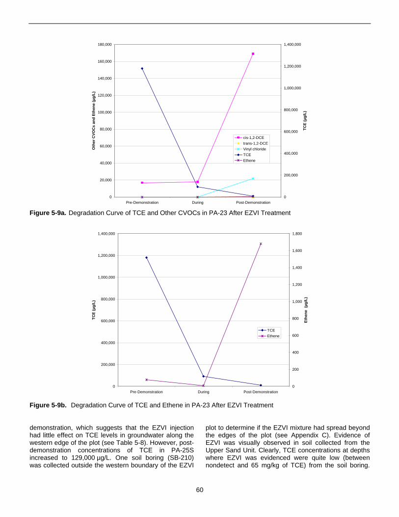
cis-1,2-DCE trans-1,2-DCE Vinyl chloride TCE Ethene

200,000 20,000

0 0 Pre-Demonstration During Post-Demonstration

180,000

160,000

140,000

120,000

100,000

80,000

1,400,000

1,200,000

1,000,000

800,000

600,000

Oth

er C

VOC

s an

d Et

hene

(µg/

L)

TCE

(µg/

L)

60,000

400,000

40,000

1,400,000

TCE Ethene

1,800

1,600 1,200,000

1,400

1,000,000

1,200

Ethe

ne (

µg/L

)

TCE

(µg/

L) 800,000 1,000

800600,000

600

400,000

400

200,000 200

0 0 Pre-Demonstration During Post-Demonstration

Figure 5-9a. Degradation Curve of TCE and Other CVOCs in PA-23 After EZVI Treatment

Figure 5-9b. Degradation Curve of TCE and Ethene in PA-23 After EZVI Treatment

demonstration, which suggests that the EZVI injection plot to determine if the EZVI mixture had spread beyond had little effect on TCE levels in groundwater along the the edges of the plot (see Appendix C). Evidence of western edge of the plot (see Table 5-8). However, post- EZVI was visually observed in soil collected from the demonstration concentrations of TCE in PA-25S Upper Sand Unit. Clearly, TCE concentrations at depths increased to 129,000 µg/L. One soil boring (SB-210) where EZVI was evidenced were quite low (between was collected outside the western boundary of the EZVI nondetect and 65 mg/kg of TCE) from the soil boring.

60

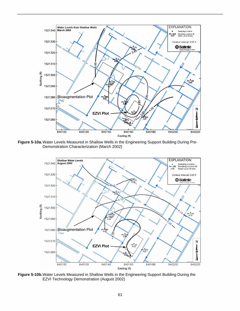
Figure 5-10a. Water Levels Measured in Shallow Wells in the Engineering Support Building During Pre-Demonstration Characterization (March 2002)

Figure 5-10b.Water Levels Measured in Shallow Wells in the Engineering Support Building During the EZVI Technology Demonstration (August 2002)

61

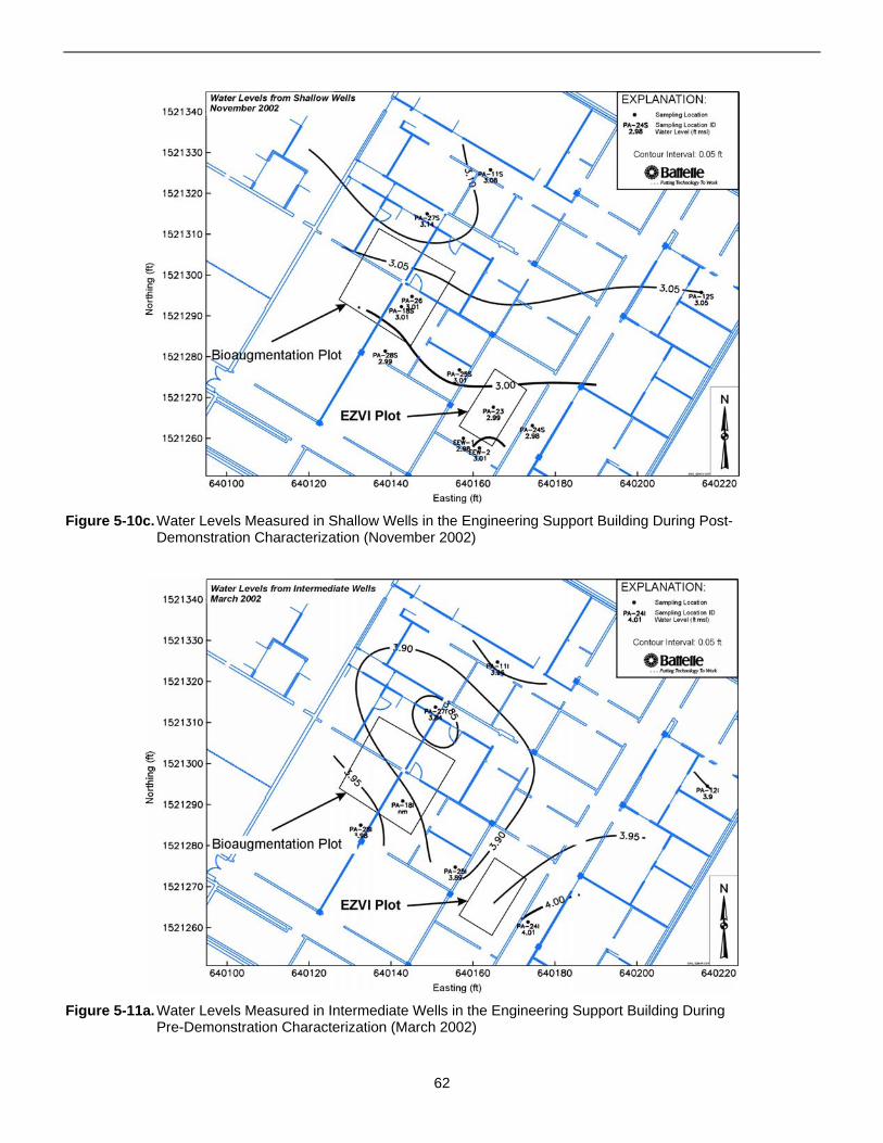
Figure 5-10c. Water Levels Measured in Shallow Wells in the Engineering Support Building During Post-Demonstration Characterization (November 2002)

Figure 5-11a. Water Levels Measured in Intermediate Wells in the Engineering Support Building During Pre-Demonstration Characterization (March 2002)

62

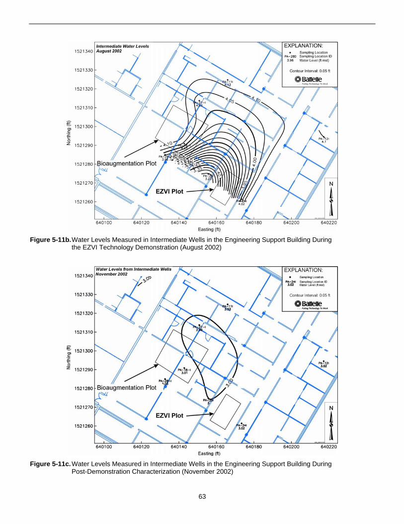
Figure 5-11b.Water Levels Measured in Intermediate Wells in the Engineering Support Building During the EZVI Technology Demonstration (August 2002)

Figure 5-11c. Water Levels Measured in Intermediate Wells in the Engineering Support Building During Post-Demonstration Characterization (November 2002)

63

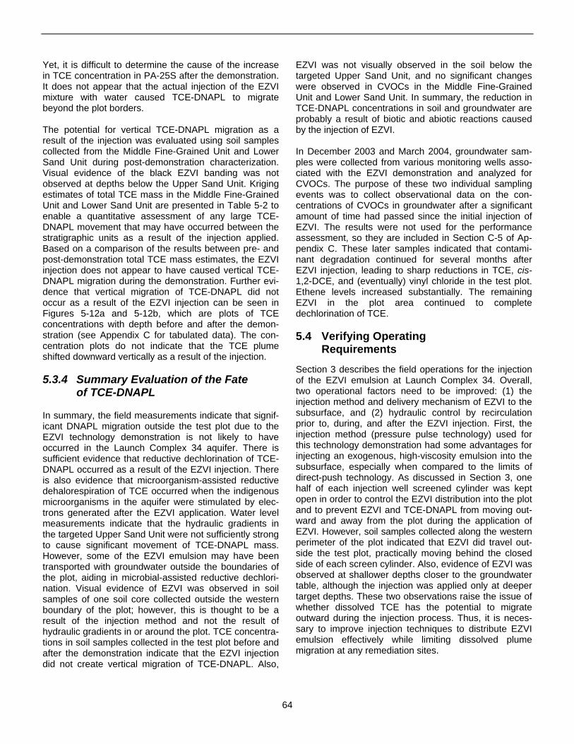
Yet, it is difficult to determine the cause of the increase in TCE concentration in PA-25S after the demonstration. It does not appear that the actual injection of the EZVI mixture with water caused TCE-DNAPL to migrate beyond the plot borders.

The potential for vertical TCE-DNAPL migration as a result of the injection was evaluated using soil samples collected from the Middle Fine-Grained Unit and Lower Sand Unit during post-demonstration characterization. Visual evidence of the black EZVI banding was not observed at depths below the Upper Sand Unit. Kriging estimates of total TCE mass in the Middle Fine-Grained Unit and Lower Sand Unit are presented in Table 5-2 to enable a quantitative assessment of any large TCE­DNAPL movement that may have occurred between the stratigraphic units as a result of the injection applied. Based on a comparison of the results between pre- and post-demonstration total TCE mass estimates, the EZVI injection does not appear to have caused vertical TCE­DNAPL migration during the demonstration. Further evi­dence that vertical migration of TCE-DNAPL did not occur as a result of the EZVI injection can be seen in Figures 5-12a and 5-12b, which are plots of TCE concentrations with depth before and after the demon­stration (see Appendix C for tabulated data). The con­centration plots do not indicate that the TCE plume shifted downward vertically as a result of the injection.

5.3.4 Summary Evaluation of the Fate of TCE-DNAPL

In summary, the field measurements indicate that signif­icant DNAPL migration outside the test plot due to the EZVI technology demonstration is not likely to have occurred in the Launch Complex 34 aquifer. There is sufficient evidence that reductive dechlorination of TCE­DNAPL occurred as a result of the EZVI injection. There is also evidence that microorganism-assisted reductive dehalorespiration of TCE occurred when the indigenous microorganisms in the aquifer were stimulated by elec­trons generated after the EZVI application. Water level measurements indicate that the hydraulic gradients in the targeted Upper Sand Unit were not sufficiently strong to cause significant movement of TCE-DNAPL mass. However, some of the EZVI emulsion may have been transported with groundwater outside the boundaries of the plot, aiding in microbial-assisted reductive dechlori­nation. Visual evidence of EZVI was observed in soil samples of one soil core collected outside the western boundary of the plot; however, this is thought to be a result of the injection method and not the result of hydraulic gradients in or around the plot. TCE concentra­tions in soil samples collected in the test plot before and after the demonstration indicate that the EZVI injection did not create vertical migration of TCE-DNAPL. Also,

EZVI was not visually observed in the soil below the targeted Upper Sand Unit, and no significant changes were observed in CVOCs in the Middle Fine-Grained Unit and Lower Sand Unit. In summary, the reduction in TCE-DNAPL concentrations in soil and groundwater are probably a result of biotic and abiotic reactions caused by the injection of EZVI.

In December 2003 and March 2004, groundwater sam­ples were collected from various monitoring wells asso­ciated with the EZVI demonstration and analyzed for CVOCs. The purpose of these two individual sampling events was to collect observational data on the con­centrations of CVOCs in groundwater after a significant amount of time had passed since the initial injection of EZVI. The results were not used for the performance assessment, so they are included in Section C-5 of Ap­pendix C. These later samples indicated that contami­nant degradation continued for several months after EZVI injection, leading to sharp reductions in TCE, cis-1,2-DCE, and (eventually) vinyl chloride in the test plot. Ethene levels increased substantially. The remaining EZVI in the plot area continued to complete dechlorination of TCE.

5.4 Verifying Operating Requirements

Section 3 describes the field operations for the injection of the EZVI emulsion at Launch Complex 34. Overall, two operational factors need to be improved: (1) the injection method and delivery mechanism of EZVI to the subsurface, and (2) hydraulic control by recirculation prior to, during, and after the EZVI injection. First, the injection method (pressure pulse technology) used for this technology demonstration had some advantages for injecting an exogenous, high-viscosity emulsion into the subsurface, especially when compared to the limits of direct-push technology. As discussed in Section 3, one half of each injection well screened cylinder was kept open in order to control the EZVI distribution into the plot and to prevent EZVI and TCE-DNAPL from moving out­ward and away from the plot during the application of EZVI. However, soil samples collected along the western perimeter of the plot indicated that EZVI did travel out­side the test plot, practically moving behind the closed side of each screen cylinder. Also, evidence of EZVI was observed at shallower depths closer to the groundwater table, although the injection was applied only at deeper target depths. These two observations raise the issue of whether dissolved TCE has the potential to migrate outward during the injection process. Thus, it is neces­sary to improve injection techniques to distribute EZVI emulsion effectively while limiting dissolved plume migration at any remediation sites.

64

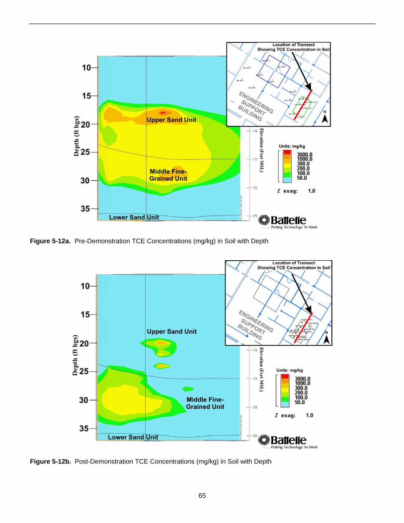
Figure 5-12a. Pre-Demonstration TCE Concentrations (mg/kg) in Soil with Depth

Figure 5-12b. Post-Demonstration TCE Concentrations (mg/kg) in Soil with Depth

65

Second, an artificial hydraulic gradient in the Upper Sand Unit was created by using two injection wells at the north end of the plot (EIW-1 and EIW-2) and two extraction wells at the south end of the plot (EEW-1 and EEW-2) to establish continuous recirculation in a rather flat aquifer and at a low flowrate. This system appeared to help advance the injected EZVI in the desired direction of treatment while controlling localized hydraulics. How­ever, water extracted from the downgradient extraction wells was not treated before reinjection into the upgra­

dient aquifer of the EZVI plot. In order to prevent intro­ducing additional contamination into the gradient aquifer, it was necessary to continuously monitor the extracted liquids from the influent and effluent sample ports of a series of two GAC vessels. The CVOC results from the effluent port of the carbon vessels in this demonstration were all below a set of guidance levels, and appeared to undergo proper treatment via GAC. Note that the proper handling of liquids is required for future applications of the EZVI technology at any remediation site.

66

6. Quality Assurance

A QAPP (Battelle, 2002a) prepared before the demon­stration outlined the performance assessment methodol­ogy and the quality assurance measures to be taken during the demonstration. The results of the field and laboratory QA for the critical soil and groundwater CVOC (primary) measurements and groundwater field param­eter (secondary) measurements are described in this section. The results of the QA measurements for both soil and groundwater sampling events are described in Ap­pendix E. The focus of the QA measures is on the critical TCE measurement in soil and groundwater, for which, in some cases, special sampling and analytical methods were used. For other measurements (chloride, calcium, etc.), standard sampling and analytical methods were used to ensure data quality.

6.1 QA Measures

This section describes the data quality in terms of repre­sentativeness and completeness of the sampling and analysis conducted for technology performance assess­ment. Chain-of-custody procedures also are described.

6.1.1 Representativeness

Representativeness is a measure that evaluates how closely the sampling and analysis represents the true value of the measured parameters in the target matrices. The critical parameter in this demonstration is TCE con­centration in soil. The following steps were taken to achieve representativeness of the soil samples:

• Statistical design for determining the number and distribution of soil samples in the 9-ft × 15-ft EZVI plot, based on the horizontal and vertical variability observed during a preliminary characterization event (see Section 4.1). Six locations (one in each cell of a 3 × 2 grid in the plot) were cored before and after the demonstration. Each continuous core was collected and sampled in 2-ft sections from the ground surface to the aquitard at most coring loca­tions except for the following: SB-8, SB-203,

SB-204, SB-207, SB-208, and SB-209. Sampling did not proceed to the aquitard for these cores either due to loss of sample during coring or because drilling to the aquitard was not required to fulfill the sampling objective. At the 80% confidence level, the reduction of TCE mass between the pre-and post-demonstration was considered to be achieved relatively well by the EZVI technology.

• Continuous sampling of the soil column at each coring location enabled the sampling design to address the vertical variability in the TCE distribu­tion. By extracting and analyzing the complete 2-ft depth in each sampled interval, essentially every vertical depth was sampled.

• Use of appropriate modifications to the standard methods for sampling and analysis of soil. To increase the representativeness of the soil sampling, the sampling and extraction procedures in U.S. EPA Method 5035 were modified so that an entire vertical section of each 2-ft core could be sampled and extracted, instead of the 5-g aliquots specified in the standard method (see Section 4.1). This was done to maximize the capture of TCE-DNAPL in the entire soil column at each coring location.

Steps taken to achieve representativeness of the ground­water samples included:

• Installation and sampling of one well in the center of the EZVI plot and two clusters of performance monitoring wells outside the plot. The well in the center was screened at the target depth in the Upper Sand Unit. Each performance well cluster consisted of three wells screened in the three strati­graphic units —Upper Sand Unit, Middle Fine-Grained Unit, and Lower Sand Unit.

• Use of standard methods for sampling and analysis. Disposable tubing was used to collect samples from all monitoring wells to avoid persistence of TCE in the sample tubing after sampling wells with high TCE (DNAPL) levels.

67

6.1.2 Completeness

All the regular samples planned in the QAPP were col­lected and analyzed, with the exception of TOC analysis from post-demonstration soil sampling. Additional soil cores outside of the EZVI plot were collected during post-demonstration sampling to evaluate the variability in the subsurface distribution of the emulsion.

All the quality control (QC) samples planned in the QAPP were collected and analyzed, except for the equipment rinsate blanks during soil coring. Equipment rinsate blanks as planned in the QAPP were collected and analyzed during the pre- or post-demonstration soil sampling events. Based on the preliminary speed of the soil coring, one rinsate blank per day was thought to be sufficient to obtain a ratio of one blank per 20 samples (5%). One rinsate blank per core was determined to be the optimum collection frequency.

6.1.3 Chain of Custody

Chain-of-custody forms were used to track each batch of samples collected in the field and were to the off-site analytical laboratory. Copies of the chain-of-custody rec­ords can be found in Appendix E. Chain-of-custody seals were affixed to each shipment of samples to ensure that only laboratory personnel accessed the samples during transit. Upon arrival at the laboratory, the laboratory veri­fied that the samples were received in good condition and the temperature blank sample sent with each ship­ment was measured to ensure that the required tem­perature was maintained during transit. Each sample received then was checked against the chain-of-custody form, and any discrepancies were brought to the atten­tion of field personnel.

6.2 Field QC Measures

The field QC checks included calibration of field instru­ments, field blanks (5% of regular samples), field dupli­cates (5% of regular samples), and trip blanks; the results of these QC checks are discussed in this section.

Table 6-1 summarizes the instruments used for field groundwater measurements (pH, ORP, DO, tempera­ture, water levels, and conductivity) and the associated calibration criteria. Instruments were calibrated at the beginning and end of the sampling period on each day. The field instruments were always within the acceptance criteria during the demonstration.

6.2.1 Field QC for Soil Sampling

As an overall determination of the extraction and ana­lytical efficiency of the soil sampling, the modified U.S. EPA Method 5035 methanol extraction procedure was evaluated in a previous demonstration at Launch Com­plex 34 by spiking a known amount of TCE into soil samples from the Launch Complex 34 aquifer. Replicate samples from the spiked soil were extracted and ana­lyzed; the results are listed in Appendix E (Table E-1). For the five replicate soil samples, the TCE spike recov­eries were in the range of 72 to 86%, which fell within the acceptable range (70-130%) for quality assurance of the extraction and analysis procedure. The results de­monstrate that a majority of the TCE was primarily extracted during the first extraction, and that diminishing returns were provided by the second and third extrac­tions (Battelle, 2002b). Based on these results, the extraction procedure defined for subsequent soil sam­pling events and subsequent demonstrations at Launch Complex 34 involved extracting one time only from the soil before sending the methanol samples to the off-site laboratory for analysis.

A more detailed evaluation of the soil extraction effi­ciency was conducted in the field during a previous steam injection/extraction technology demonstration at Launch Complex 34 by spiking a surrogate compound (1,1,1-TCA) directly into the intact soil cores retrieved in a sleeve (Battelle, 2002b). The injection volume of 1,1,1­TCA was approximately 10 µL. The spiked soil samples were handled in the same manner as the remaining soil samples during the extraction procedure. Extraction efficiencies for the experiment ranged from 84 to 113%. The results of the experiment were compared to the

Table 6-1. Instruments and Calibration Acceptance Criteria Used for Field Measurements

68

Instrument Measurement Acceptance Criteria YSI Meter Model 6820 pH 3 point, ±20% difference YSI Meter Model 6820 ORP 1 point, ±20% difference YSI Meter Model 6820 Conductivity 1 point, ±20% difference YSI Meter Model 6820 Dissolved Oxygen 1 point, ±20% difference YSI Meter Model 6820 Temperature 1 point, ±20% difference OHaus Weight Balance Soil – Dry/Wet Weight 3 point, ±20% difference Hermit Water Level Indicator Water Levels ±0.01 ft

results of the post-demonstration soil characterization, where soil samples also were spiked with 1,1,1-TCA. Of the 13 soil samples spiked with 1,1,1-TCA during the steam injection demonstration at Launch Complex 34, 12 soil samples were within the acceptable range of precision for the post-demonstration soil sampling, cal­culated as the relative percent difference (RPD), where RPD is less than 30% (Table E-2). The results indicate that the methanol extraction procedure used in the field is suitable for recovering CVOCs.

During the EZVI pre- and post-demonstration sampling events, duplicate soil samples were collected in the field and analyzed for TCE to evaluate sampling precision. Duplicate soil samples were collected by splitting each 2-ft soil core vertically in half and subsequently collecting approximately 250 g of soil into two separate containers, marked as SB#-Depth# and SB#-Depth#-DUP. Appen­dix E (Table E-3) shows the result of the field soil dupli­cate analysis and the precision, calculated as the RPD for the duplicate soil cores, which were collected before and after the demonstration. The precision of the field duplicate samples was generally within the acceptable range (RPD<30%) for the demonstration, indicating that the sampling procedure was representative of the soil column at the coring location. The RPD for one of the duplicate soil samples from the pre-demonstration sam­pling was greater than 30%, which indicated that the repeatability of some of the pre-demonstration soil sam­ples was outside targeted acceptance criteria. However, given the heterogeneous nature of the contaminant dis­tribution, a large RPD on occasion is not unexpected. The RPDs for three of the duplicate soil samples from the post-demonstration sampling were greater than 30%. This suggests that the EZVI treatment created greater variability in the contaminant distribution. Part of the rea­son for the higher RPD calculated in some post-demon­stration soil samples is that TCE concentrations tended to be low (often near or below the detection limit). For example, the RPD between duplicate samples, one of which is below detection and the other is slightly above detection, tends to be high. In general, though, the vari­ability in the two vertical halves of each 2-ft core was in a reasonable range, given the typically heterogeneous nature of the DNAPL distribution.

Field blanks for the soil sampling consisted of rinsate blank samples and methanol blank samples. The rinsate blank samples were collected approximately once per drilling borehole, or approximately once per 20 soil samples, to evaluate the decontamination efficiency of the sampling equipment used to collect each soil sam­ple. Decontamination between samples consisted of a three-step process where the sampling equipment was washed with soapy water, rinsed in distilled water to remove soap and debris, and then rinsed a second time

with distilled water. The rinsate blank samples were collected by pouring distilled water over the equipment after the equipment had been processed through the routine decontamination procedure. As seen in Appen­dix E (Table E-4), TCE levels in the rinsate blanks were below detection (<1.0 µg/L) for all but one of the 15 rins­ate blanks collected, indicating that the decontamination procedure was helping control carryover of CVOCs between samples.

Methanol blank samples were collected in the field at the rate of one per soil boring, or approximately every 20 samples (5%), to evaluate the soil extraction process. The results are listed in Appendix E (Table E-5). These samples were generally below the targeted detection limit of 100 µg/L of TCE in methanol. Detectable levels of TCE were present in methanol blanks collected during the post-demonstration phase of the project, but were still relatively low. Because several of the methanol blanks with detectable levels of TCE were collected dur­ing the same sampling event in October 2002, it is pos­sible that the methanol may have become contaminated during storage at the site. However, the TCE concentra­tions in these blanks were generally below 10% of the concentrations in the associated batch of soil samples. All the pre-demonstration methanol blanks were below detection.

Trip blanks were sent with every sample shipment, both soil and groundwater, to the off-site analytical laboratory. The results are discussed in Section 6.2.2.

6.2.2 Field QC for Groundwater Sampling

QC checks for groundwater sampling included field dup­licates (5%), field blanks (5%), and trip blanks. Field duplicate samples were collected once per sampling event, or approximately once per eight to ten wells sam­pled. Appendix E (Table E-6) contains the analysis of the field duplicate groundwater samples that were collected before, during, and after the demonstration. The RPD (precision) calculated for these samples always met the QA/QC target criteria of RPD<30%.

In previous demonstrations carried out at Launch Com­plex 34, decontamination of the sample tubing between groundwater samples initially consisted of a detergent rinse and two distilled water rinses. However, the results from these earlier demonstrations revealed that, despite the most thorough decontamination, rinsate blanks con­tained elevated levels of TCE, especially following the sampling of wells containing TCE levels near or greater than its solubility (1,100,000 µg/L); this indicated that some free-phase solvent may have been drawn into the

69

tubing. When TCE levels in such rinsate blanks refused to go down, even when a methanol rinse was added to the decontamination procedure, a decision was made to switch to disposable Teflon® tubing. All groundwater sam­pling events conducted for the EZVI demonstration used disposable Teflon® tubing. Each new piece of tubing was used for sampling each well once and then discarded, despite the associated costs. TCE levels in the rinsate blanks (Appendix E, Table E-7) were below the targeted detection limit (3.0 µg/L) throughout the demonstration.

Trip blanks supplied by the off-site laboratory were included for CVOC analysis with every sample shipment sent to the laboratory. TCE levels in trip blank samples were below the QA/QC target level of 3 µg/L for 17 of the 19 trip blanks analyzed for the demonstration (Ap­pendix E, Table E-8). Of the two trip blanks that failed to meet the target level, the laboratory was able to deter­mine that the trip blanks were part of an older batch of blanks sent to the site during the previous month and concluded that the trip blanks had become contaminated during storage at the site and not during shipment.

6.3 Laboratory QC Measures

The off-site analytical laboratories performed QA/QC checks consisting of 5% matrix spikes (MS) and matrix spike duplicates (MSD). MS and MSD were used to calculate analytical accuracy (percent recovery) and pre­cision (RPD between MS and MSD). Laboratory control spikes (LCS) and method blanks (MB) also were ana­lyzed with every batch of samples.

6.3.1 Analytical QC for Soil Sampling

Analytical accuracy for the soil samples (methanol extracts) analyzed were generally within acceptance limits for TCE (70-130%) for the pre- and post-demon­stration period (Appendix E, Tables E-9 and E-10). Matrix spike recoveries were outside this range for three of the MS/MSD samples conducted during the pre-demonstration sampling period, and three during the post-demonstration period. The spike recovery was out­side of the control limits due to either very high or very low (i.e., near detection limit) concentrations of TCE present in the reference sample. No corrective actions were required and sample results were not adversely affected by the MS/MSD spike recoveries that were out­side the control limits. The precision between MS and MSD was always within acceptance limits (RPD <30%). Laboratory control spike recoveries for all pre- and post-demonstration samples were within the acceptance cri­teria (Appendix E, Table E-11).

Method blanks were below the target level of 3.0 µg/L for TCE for 40 of the 41 method blanks analyzed during pre- and post-demonstration sampling. The single sample that did not meet the criteria was measured with a TCE recovery <1,000 µg/L due to a change in the method detection limit for that sample; therefore it is unknown if that particular method blank met the QA/QC target cri­teria (Appendix E, Table E-12).

The laboratory conducted surrogate spikes in 5% of the total number of methanol extracts prepared from the soil samples for CVOC analysis. Table 6-2 lists the surrogate compounds used by the laboratory to perform the QA/ QC checks. Surrogate recoveries were within the speci­fied acceptance limits.

Table 6-2. List of Surrogate Compounds and Their Target Recoveries for Soil and Ground­water Analysis by the Analytical Laboratory

Surrogate Compound

Target Recovery for Soil

(Methanol Extracts) (%)

Target Recovery for Groundwater

(%) Dibromofluoromethane 65-135 75-125 1,2-Dichloroethane – d4 52-149 62-139 Toluene – d8 65-135 75-125 Bromofluorobenzene 65-135 75-125

6.3.2 Laboratory QC for Groundwater Sampling

Pre- and post-demonstration MS and MSD results for groundwater are listed in Appendix E (Table E-13). The MS and MSD recoveries (75 to 125%) were generally within acceptance criteria. The only exceptions were one MS/MSD sample set during the demonstration and one MS/MSD sample set during post-demonstration ground­water sampling. The spike recovery was outside of the control limits due to either very high or very low (i.e., near detection limit) concentrations of TCE present in the reference sample. No corrective actions were required and sample results were not adversely affected by the MS/MSD spike recoveries that were outside the control limits. The precision for all of the MS/MSD sam­ples met the QA/QC criteria of RPD <20%. Recoveries for LCS samples were always within the acceptance range of 75-125% (Appendix E, Table E-14).

Method blanks (Appendix E, Table E-15) for the ground­water samples were always below the targeted 3.0 µg/L detection limit.

70

6.3.3 Analytical Detection Limits

Detection limits for TCE in groundwater and in the meth­anol extracts from soil generally were met. The detection limits most affected were those for cis-1,2-DCE and VC, due to the masking effect of high levels of TCE. The laboratories verified and reported that analytical instru­mentation calibrations were within an acceptable range on the days of the analyses.

6.4 QA/QC Summary

Given the challenges posed by the typically heterogene­ous TCE distribution in a DNAPL source zone, the col­lected data were an acceptable representation of the TCE distribution in the Launch Complex 34 aquifer before, during, and after the demonstration.

• Six spatially distributed locations were sampled within the plot to adequately capture the horizontal variability in the TCE distribution. The continuous sampling of the soil at each coring location ensured that the vertical variability of the TCE distribution was captured. Sampling and analytical procedures were appropriately modified to address the expected

variability. Standard sampling and analysis methods were used for all other measurements to ensure that data were comparable between sampling events.

• Accuracy and precision of the soil and groundwater measurements were generally in the acceptable range for the field sampling and laboratory analysis. In the few instances that QC data were outside the targeted range, the reason was generally interfer­ence from extremely low (near detection) or extremely high levels of TCE in the sample that caused higher deviation in the precision (repeat­ability) of the data.

• The masking effect of high TCE levels on other CVOCs and the need for sample dilution as a result caused detection limits for TCE to rise in certain instances. However, because the surrogate recov­eries were all within acceptable range, the rise in detection limits did not interfere with reporting acceptable CVOC concentrations.

• Rinsate blanks associated with the soil and ground­water samples generally had acceptably low or undetected levels of TCE.

71

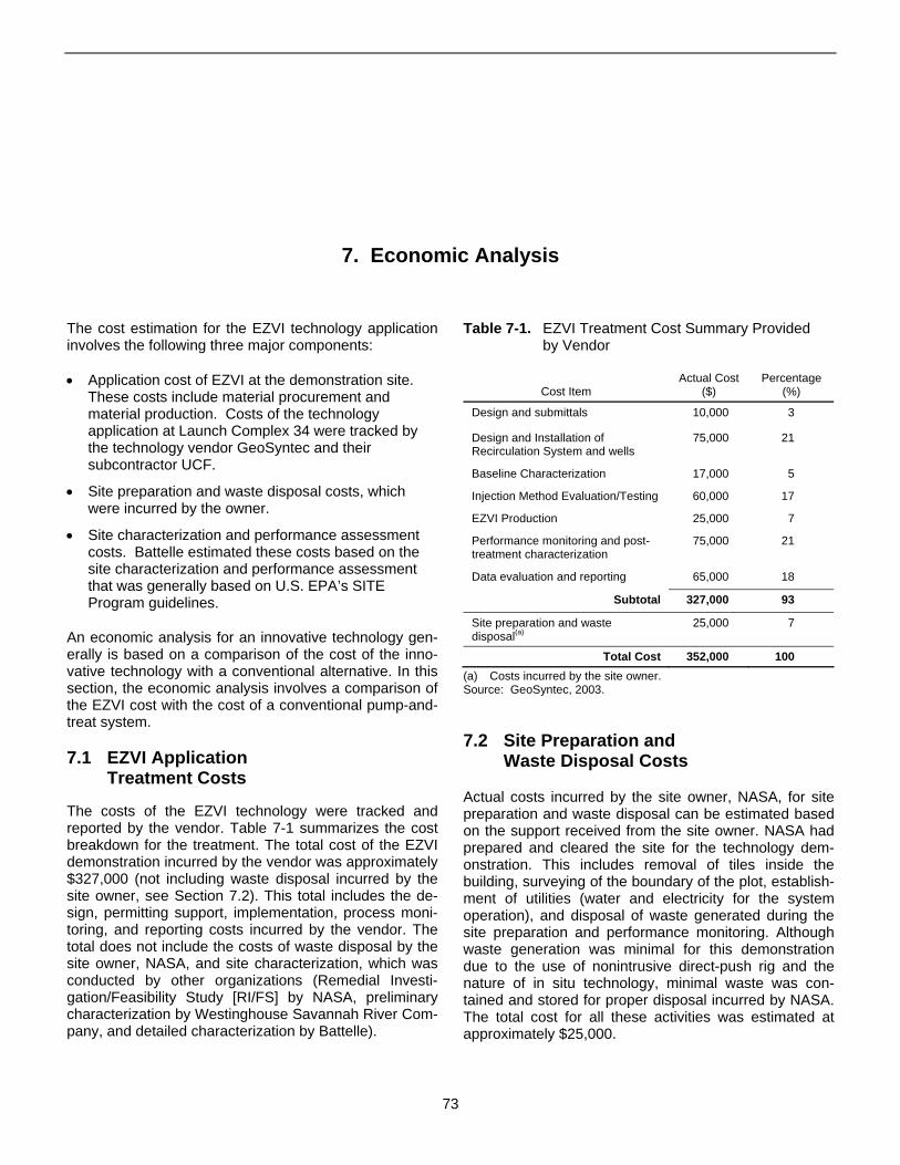
7. Economic Analysis

The cost estimation for the EZVI technology application involves the following three major components:

• Application cost of EZVI at the demonstration site. These costs include material procurement and material production. Costs of the technology application at Launch Complex 34 were tracked by the technology vendor GeoSyntec and their subcontractor UCF.

• Site preparation and waste disposal costs, which were incurred by the owner.

• Site characterization and performance assessment costs. Battelle estimated these costs based on the site characterization and performance assessment that was generally based on U.S. EPA’s SITE Program guidelines.

An economic analysis for an innovative technology gen­erally is based on a comparison of the cost of the inno­vative technology with a conventional alternative. In this section, the economic analysis involves a comparison of the EZVI cost with the cost of a conventional pump-and­treat system.

7.1 EZVI Application Treatment Costs

The costs of the EZVI technology were tracked and reported by the vendor. Table 7-1 summarizes the cost breakdown for the treatment. The total cost of the EZVI demonstration incurred by the vendor was approximately $327,000 (not including waste disposal incurred by the site owner, see Section 7.2). This total includes the de­sign, permitting support, implementation, process moni­toring, and reporting costs incurred by the vendor. The total does not include the costs of waste disposal by the site owner, NASA, and site characterization, which was conducted by other organizations (Remedial Investi­gation/Feasibility Study [RI/FS] by NASA, preliminary characterization by Westinghouse Savannah River Com­pany, and detailed characterization by Battelle).

Table 7-1. EZVI Treatment Cost Summary Provided by Vendor

Cost Item Actual Cost

($) Percentage

(%)

Design and submittals 10,000 3

Design and Installation of 75,000 21 Recirculation System and wells

Baseline Characterization 17,000 5

Injection Method Evaluation/Testing 60,000 17

EZVI Production 25,000 7

Performance monitoring and post- 75,000 21 treatment characterization

Data evaluation and reporting 65,000 18

Subtotal 327,000 93

Site preparation and waste disposal(a)

25,000 7

Total Cost 352,000 100 (a) Costs incurred by the site owner. Source: GeoSyntec, 2003.

7.2 Site Preparation and Waste Disposal Costs

Actual costs incurred by the site owner, NASA, for site preparation and waste disposal can be estimated based on the support received from the site owner. NASA had prepared and cleared the site for the technology dem­onstration. This includes removal of tiles inside the building, surveying of the boundary of the plot, establish­ment of utilities (water and electricity for the system operation), and disposal of waste generated during the site preparation and performance monitoring. Although waste generation was minimal for this demonstration due to the use of nonintrusive direct-push rig and the nature of in situ technology, minimal waste was con­tained and stored for proper disposal incurred by NASA. The total cost for all these activities was estimated at approximately $25,000.

73

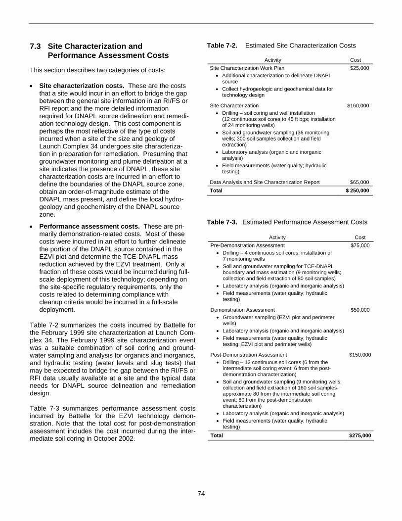
7.3 Site Characterization and Performance Assessment Costs

This section describes two categories of costs:

• Site characterization costs. These are the costs that a site would incur in an effort to bridge the gap between the general site information in an RI/FS or RFI report and the more detailed information required for DNAPL source delineation and remedi­ation technology design. This cost component is perhaps the most reflective of the type of costs incurred when a site of the size and geology of Launch Complex 34 undergoes site characteriza­tion in preparation for remediation. Presuming that groundwater monitoring and plume delineation at a site indicates the presence of DNAPL, these site characterization costs are incurred in an effort to define the boundaries of the DNAPL source zone, obtain an order-of-magnitude estimate of the DNAPL mass present, and define the local hydro-geology and geochemistry of the DNAPL source zone.

• Performance assessment costs. These are pri­marily demonstration-related costs. Most of these costs were incurred in an effort to further delineate the portion of the DNAPL source contained in the EZVI plot and determine the TCE-DNAPL mass reduction achieved by the EZVI treatment. Only a fraction of these costs would be incurred during full-scale deployment of this technology; depending on the site-specific regulatory requirements, only the costs related to determining compliance with cleanup criteria would be incurred in a full-scale deployment.

Table 7-2 summarizes the costs incurred by Battelle for the February 1999 site characterization at Launch Com­plex 34. The February 1999 site characterization event was a suitable combination of soil coring and ground­water sampling and analysis for organics and inorganics, and hydraulic testing (water levels and slug tests) that may be expected to bridge the gap between the RI/FS or RFI data usually available at a site and the typical data needs for DNAPL source delineation and remediation design.

Table 7-3 summarizes performance assessment costs incurred by Battelle for the EZVI technology demon­stration. Note that the total cost for post-demonstration assessment includes the cost incurred during the inter­mediate soil coring in October 2002.

Table 7-2. Estimated Site Characterization Costs

Activity Cost Site Characterization Work Plan $25,000

• Additional characterization to delineate DNAPL source

• Collect hydrogeologic and geochemical data for technology design

Site Characterization $160,000 • Drilling – soil coring and well installation

(12 continuous soil cores to 45 ft bgs; installation of 24 monitoring wells)

• Soil and groundwater sampling (36 monitoring wells; 300 soil samples collection and field extraction)

• Laboratory analysis (organic and inorganic analysis)

• Field measurements (water quality; hydraulic testing)

Data Analysis and Site Characterization Report $65,000 Total $ 250,000

Table 7-3. Estimated Performance Assessment Costs

Activity Cost Pre-Demonstration Assessment $75,000

• Drilling – 4 continuous soil cores; installation of 7 monitoring wells

• Soil and groundwater sampling for TCE-DNAPL boundary and mass estimation (9 monitoring wells; collection and field extraction of 80 soil samples)

• Laboratory analysis (organic and inorganic analysis) • Field measurements (water quality; hydraulic

testing)

Demonstration Assessment $50,000 • Groundwater sampling (EZVI plot and perimeter

wells)• Laboratory analysis (organic and inorganic analysis) • Field measurements (water quality; hydraulic

testing; EZVI plot and perimeter wells)

Post-Demonstration Assessment $150,000 • Drilling – 12 continuous soil cores (6 from the

intermediate soil coring event; 6 from the post-demonstration characterization)

• Soil and groundwater sampling (9 monitoring wells; collection and field extraction of 160 soil samples-approximate 80 from the intermediate soil coring event; 80 from the post-demonstration characterization)

• Laboratory analysis (organic and inorganic analysis) • Field measurements (water quality; hydraulic

testing) Total $275,000

74

7.4 Present Value Analysis of EZVI Technology and Pump-and-Treat System Costs

DNAPL, especially of the magnitude present at Launch Complex 34, is likely to persist in the aquifer for several decades or centuries. The resulting groundwater contami­nation and plume also will persist for several decades. The conventional approach to this type of contamination has been the use of pump-and-treat systems that extract and treat the groundwater above ground. This conven­tional technology is basically a plume control technology and would have to be implemented as long as ground­water contamination exists. The EZVI application tech­nology is an innovative in situ technology that may be comparable to the conventional pump-and-treat approach. The economic analysis therefore compares the costs of these two alternatives.

Because a pump-and-treat system would have to be operated for the next several decades, the life-cycle cost of this long-term treatment has to be calculated and compared with the cost of the EZVI treatment technol­ogy, a short-term treatment. The present value (PV) of a long-term pump-and-treat application is calculated as described in Appendix F. The PV analysis is conducted over a 30-year period, as is typical for long-term remedi­ation programs at Superfund sites. Site characterization and performance (compliance) assessment costs are assumed to be the same for both alternatives and are not included in this analysis.

For the purpose of comparison, it is assumed that a pump-and-treat system would have to treat the plume emanating from a DNAPL source. However, the demon­stration was limited to a plot that was 9-ft wide × 15-ft long × 30-ft deep. For a more realistic cost comparison, the remediation site is assumed to be spatially three times bigger (27-ft wide × 45-ft long × 30-ft deep) than the EZVI plot for this cost evaluation. Recent research (Pankow and Cherry, 1996) indicates that the most effi­cient pump-and-treat system for source containment would capture all the groundwater flowing through the DNAPL source region. For a 27-ft-long × 45-ft-wide × 30-ft-deep (Upper Sand Unit) DNAPL source region at Launch Complex 34, a single extraction well pumping at 2 gpm is assumed to be sufficient to contain the source in an aquifer where the hydraulic gradient (and therefore, the groundwater flow velocity) is extremely low. This type of minimal containment pumping ensures that the source is contained without having to extract and treat groundwater from cleaner surrounding regions, as would be the case in more aggressive conventional pump-and­treat systems. The extracted groundwater is treated with an air stripper, polishing carbon (liquid phase), and a catalytic oxidation unit (for air effluent).

As shown in Tables F-1 and F-2 of Appendix F, the total capital investment for an equivalent pump-and-treat sys­tem would be approximately $161,000, and would be fol­lowed by an annual operation and maintenance (O&M) cost of $50,000 (including quarterly monitoring). Periodic maintenance requirements (replacements of pumps, etc.) would raise the O&M cost every five years to $69,000 and every 10 years to $97,000. A discount rate (real rate of return) of 2.9%, based on the current recom­mendation for government projects, was used to calcu­late the PV. The PV of the pump-and-treat costs over 30 years is estimated to be $1,365,000.

An equivalent treatment cost for full-scale deployment of the EZVI treatment technology in a source area approxi­mately for the same size of treatment area as the one used for the pump-and-treat system would be at least $452,000. This estimate is based on a total EZVI treat­ment ($352,000 [see Table 7-1]) incurred for the dem­onstration. The assumed dimension to be treated is approximately three times of the EZVI plot. An equal number (8) of injection wells could be used for the injec­tion, and twice as much of the EZVI could be used in the source treatment, although two additional volumes of waste would be generated. Additional costs of $100,000 would be necessary for the additional EZVI production cost ($25,000 times two) and waste disposal cost ($25,000 times two) based on the demonstration cost in Table 7-1. Therefore, if the TCE remaining after EZVI treatment was allowed to attenuate naturally, the total treatment cost with the EZVI technology would be ap­proximately $452,000. Given the presence of vegetable oil residuals from the EZVI, a slow-release carbon source is available to aid biodegradation of TCE residu­als. Another assumption here is that the full-scale deployment of the EZVI treatment system would entail design, equipment, and deployment similar to the kind done during the demonstration.

Therefore, the EZVI treatment technology is cost-competitive with an equivalent pump-and-treat system. An investment in the EZVI treatment has a lower PV than the long-term investment in a pump-and-treat sys­tem. The up-front capital investment incurred for the EZVI treatment may by recovered after the fifth year (see Table F-3 in Appendix F), when the PV of the pump-and­treat system surpasses the cost of the EZVI treatment.

In addition to a lower PV or life-cycle cost, there may be other tangible and intangible economic benefits to using a source remediation technology. For example, the eco­nomic analysis in Appendix F assumes that the pump-and-treat system is operational at all times over the next 30 years or more, with most of the annual expense associated with operation and routine (scheduled) main­tenance. Experience with pump-and-treat systems at several sites has shown that downtime associated with

75

pump-and-treat systems is fairly high (as much as 50% downtime reported from some sites). This may nega­tively impact both maintenance requirements (tangible cost) and the integrity of plume containment (intangible cost) with the pump-and-treat alternative.

Another factor to consider is that although the economic analysis for long-term remediation programs typically is conducted for a 30-year period, the DNAPL source and therefore the pump-and-treat requirement may persist

for many more years or decades. This would lead to concomitantly higher remediation costs for the pump-and-treat or plume containment option (without source removal). As seen in Appendix F, the PV of a pump-and-treat system operated for 100 years would be $2,126,000. Even if the DNAPL source is only partially removed by the EZVI treatment, and natural attenuation is insufficient to meet downgradient cleanup goals, it is anticipated that the reduced source leads to a reduction in the size and timeframe for a pump-and-treat system.

76

8. Technology Applications Analysis

This section evaluates the general applicability of the EZVI technology to sites with contaminated groundwater and soil. The analysis is based on the results and les­sons learned from the demonstration, as well as general information available about the technology and its appli­cation at other sites.

8.1 Objectives

This section evaluates the EZVI technology against the nine evaluation criteria used for detailed analysis of remedial alternatives in feasibility studies under the Comprehensive Environmental Response, Compensa­tion, and Liability Act (CERCLA). Much of the discussion in this section applies to DNAPL source removal in gen­eral and the EZVI technology in particular.

8.1.1 Overall Protection of Human Health and the Environment

EZVI is protective of human health and environment in both the short and long term. Because DNAPL acts as a secondary source that can contaminate an aquifer for decades or centuries, DNAPL source removal or mitiga­tion considerably reduces the duration over which the source is active. Even if DNAPL mass removal is not 100%, the resulting long-term weakening of the plume and the reduced duration over which the DNAPL source contributes to the plume reduces the threat to potential receptors.

8.1.2 Compliance with ARARs

This section describes the technology performance ver­sus applicable or relevant and appropriate requirements (ARARs). Compliance with location-, action-, and chemical-specific ARARs should be determined on a site-specific basis. Location-specific ARARs may apply during a remediation project if the technology has the potential to affect resources in and around the site

location. Examples of resources that fall under location-specific ARARs include cultural resources, biological resources, flood plains and wetlands, hydrologic resources, and critical habitat. In general, the design of the EZVI technology is flexible enough that location-specific ARARs could be met.

Action-specific ARARs correspond to waste discharge requirements associated with the technology, such as discharging to the air or hazardous waste generation, management, and disposal. In general, action-specific ARARs could be met with the EZVI technology. One advantage of the EZVI technology is the potential for the emulsion to be injected without the accompanying recir­culating groundwater system. The recirculating system produces groundwater that must be treated prior to rein­jection according to the requirements of RCRA 3020(b) (U.S. EPA, 2000). Further testing of the EZVI technology is necessary to optimize injection strategies in the absence of a recirculating groundwater system.

Chemical-specific ARARs are generally health- or risk-based numerical values or methodologies applied to site-specific conditions that result in the establishment of a cleanup level. Compliance with chemical-specific ARARs depends on the efficiency of the EZVI process at the site and the cleanup goals agreed on by various stakehold­ers. In general, reasonable DNAPL mass removal goals are more achievable and should lead to eventual and earlier compliance with long-term groundwater cleanup goals. Achieving short-term groundwater cleanup goals (e.g., federal or state maximum contaminant levels [MCLs]), especially in the DNAPL source zone, is more difficult because various studies (Pankow and Cherry, 1996) have shown that almost 100% DNAPL mass removal may be required before a significant change in groundwater concentrations is observed. However, removal of DNAPL, even if most of the removal takes place from the more accessible pores, probably would result in a weakened plume that may allow risk-based cleanup goals to be met in the downgradient aquifer.

77

The specific federal environmental regulations that are potentially impacted by remediation of a DNAPL source with EZVI are described below.

8.1.2.1 Comprehensive Environmental Response, Compensation, and Liability Act

CERCLA, as amended by the Superfund Amendment and Reauthorization Act (SARA), provides for federal authority to respond to releases or potential releases of any hazardous substance into the environment, as well as to releases of pollutants or contaminants that may present an imminent or significant danger to public health and welfare or the environment. Remedial alter­natives that significantly reduce the volume, toxicity, or mobility of hazardous materials and that provide long-term protection are preferred. Selected remedies also must be cost-effective and protective of human health and the environment. The EZVI technology meets sev­eral of these criteria relating to a preferred alternative. EZVI reduces the toxicity of chlorinated contaminants by converting them into potentially nontoxic forms. For example, at Launch Complex 34, as described in Sec­tion 5.3.1, increases in ethene and chloride concentra­tions in groundwater collected during post-demonstration characterization indicate that some portion of the TCE was converted into nontoxic forms by the EZVI treat­ment. This elimination of solvent hazard is permanent and leads to a considerable reduction in the time it takes for the DNAPL source to deplete fully. Although aquifer heterogeneities and technology limitations often result in less than 100% (complete) removal of the contaminant and elevated levels of dissolved solvent may persist in the groundwater over the short term, there is faster and eventual elimination of groundwater contamination in the long term. Section 7.4 shows that EZVI technology is cost-effective compared with the conventional alternative of long-term pump and treat.

8.1.2.2 Resource Conservation and Recovery Act

RCRA, as amended by the Hazardous and Solid Waste Amendments (HSWA) of 1984, regulates management and disposal of municipal and industrial solid wastes. The U.S. EPA and RCRA-authorized states (listed in 40 CFR Part 272) implement and enforce RCRA and state regulations. Generally, RCRA does not apply to in situ groundwater treatment because the contaminated groundwater may not be considered hazardous waste while it is still in the aquifer. The contaminated ground­water becomes regulated if it is extracted from the ground, as would happen with the conventional alternative of pump and treat. At Launch Complex 34, the recirculation system required for hydraulic control of the test plot necessitated treatment of the extracted groundwater

prior to reinjection. At similar sites, and under similar cir­cumstances, RCRA may be invoked as an ARAR.

8.1.2.3 Clean Water Act

The CWA is designed to restore and maintain the chem­ical, physical, and biological quality of navigable surface waters by establishing federal, state, and local discharge standards. The CWA may apply if groundwater extrac­tion is conducted in conjunction with EZVI injection, and the resulting water stream needs to be treated and dis­charged to a surface water body or a publicly owned treatment works (POTW). On-site discharges to a sur­face water body must meet National Pollutant Discharge Elimination System (NPDES) requirements; consequent­ly, an NPDES permit may be needed under the NPDES requirements. Off-site discharges to a surface water body must meet NPDES limits and require an NPDES permit. Discharge to a POTW, even if it is through an on-site sewer, is considered an off-site activity and requires an NPDES permit. Sometimes, soil or groundwater mon­itoring may lead to small amounts of purge and decon­tamination water wastes that may be subject to CWA requirements. Micropurging was one measure imple­mented at Launch Complex 34 to minimize such wastes during site characterization and technology performance assessment.

8.1.2.4 Safe Drinking Water Act

The SDWA, as amended in 1986, requires U.S. EPA to establish regulations to protect human health from con­taminants in drinking water. The legislation authorizes national drinking water standards and a joint federal-state system for ensuring compliance with these stand­ards. The SDWA also regulates underground injection of fluids through the Underground Injection Control (UIC) Program and includes sole-source aquifer and wellhead protection programs. A UIC variance was obtained from the FDEP to inject the EZVI into the aquifer during this demonstration.

The National Primary Drinking Water Standards are found at 40 CFR Parts 141 through 149. The health-based SDWA primary standards (e.g., MCL) are more critical to meet; SDWA secondary standards (e.g., for iron, chloride, or TDS) are based on other factors, such as aesthetics (discoloration) or odor. The MCLs based on these standards generally apply as cleanup stand­ards for water that is, or potentially could be, used for drinking water supply. In some cases, such as when multiple contaminants are present, alternative concentra­tion limits (ACLs) may be used. CERCLA and RCRA standards and guidance are used in establishing ACLs. In addition, some states may set more stringent stand­ards for specific contaminants. For example, the federally mandated MCL for VC is 2 µg/L, whereas the State of

78

Florida drinking water standard is 1 µg/L. In such instances, the more stringent standard is usually the cleanup goal.

Although the long-term goal of DNAPL source zone treatment is meeting applicable drinking water standards or other risk-based groundwater cleanup goals agreed on between site owners and regulatory authorities, the short-term objective of the EZVI technology and source remediation is DNAPL mass removal. Because technol­ogy, site, and economic limitations may limit DNAPL mass removal to less than 100%, it may not always be possible to meet groundwater cleanup targets in the source region in the short term. Depending on other fac­tors, such as the distance of the compliance point (e.g., property boundary, at which groundwater cleanup tar­gets have to be met) from the source (as negotiated between the site owner and regulators), the degree of weakening of the plume due to DNAPL source treat­ment, and the degree of natural attenuation in the aqui­fer, it may be possible to meet groundwater cleanup targets at the compliance point in the short term. DNAPL mass removal will always lead to faster attainment of groundwater cleanup goals in the long term, as com­pared to the condition in which no source removal action is taken.

One aspect of using EZVI as a reductant for DNAPL source remediation is the potential for an increase in iron concentrations in groundwater as a result of the treat­ment. Iron is a secondary drinking water standard under the SDWA, with a maximum concentration of 0.3 mg/L. At Launch Complex 34, the concentrations of dissolved iron measured in the shallow monitoring wells during the pre-demonstration characterization were much higher than the secondary drinking water standard, and ranged from 7.2 to 27 mg/L (see Table 5-5). Total iron con­centrations were approximately the same as those for dissolved iron, indicating that dissolved iron is the pre­dominant form in the aquifer. Both total and dissolved iron concentrations decreased after the EZVI injection. Precipitation of ferric iron on soil was not observed visu­ally (as tan color) during post-demonstration character­ization, but a full microscopic analysis of the soil was not conducted to verify the presence of precipitates. The post-demonstration data were inconclusive regarding the impact of the EZVI technology on iron concentrations in the targeted Upper Sand Unit following the EZVI injection. However, because the shallow aquifer at Launch Com­plex 34 is not used for drinking water, the secondary standard for iron did not apply to the EZVI demonstration.

8.1.2.5 Clean Air Act

The CAA and the 1990 amendments establish primary and secondary ambient air quality standards for protection

of public health, as well as emission limitations for cer­tain hazardous pollutants. Permitting requirements under CAA are administered by each state as part of State Implementation Plans (SIPs) developed to bring each state in compliance with National Ambient Air Quality Standards (NAAQS).

Unlike pump-and-treat systems, which often generate air emissions (when an air stripper is used), and unlike other source removal technologies that use thermal energy (e.g., steam injection or resistive heating) or result in exothermic reactions (e.g., oxidation with Fen-ton’s reagent), the potential for atmospheric releases is absent when injecting EZVI.

8.1.2.6 Occupational Safety and Health Administration

CERCLA remedial actions and RCRA corrective actions must be carried out in accordance with Occupational Safety and Health Administration (OSHA) requirements detailed in 20 CFR Parts 1900 through 1926, especially Part 1910.120, which provide for the health and safety of workers at hazardous waste sites. On-site construction activities at Superfund or RCRA corrective action sites must be performed in accordance with Part 1926 of RCRA, which provides safety and health regulations for construction sites. State OSHA requirements, which may be significantly stricter than federal standards, also must be met.

The health and safety aspects of EZVI injection are mini­mal. The main working hazards encountered during the demonstration were operating heavy equipment (e.g., drill rig) and handling the emulsified iron mixture. These hazards were dealt with by using trained personnel and appropriate personal protective equipment. Level D per­sonal protective equipment generally would be sufficient during implementation. During the injection phase of the demonstration, Tyvek® suits were worn to prevent work­ers’ clothing from being covered in the emulsion. All operating and sampling personnel were required to have completed the 40-hour Hazardous Waste Operations training course and 8-hour refresher courses.

8.1.3 Long-Term Effectiveness

The EZVI technology leads to removal of TCE-DNAPL mass and therefore permanent removal of contamination from the aquifer. Although dissolved solvent concentra­tions may rebound in the short term when groundwater flow redistributes through the treated source zone con­taining DNAPL remnants, depletion of the source through dissolution will continue in the long term, and lead to eventual and earlier compliance with ground­water cleanup goals.

79

8.1.4 Reduction of Toxicity, Mobility, or Volume through Treatment

The EZVI technology effects treatment by reducing the volume and toxicity of contamination through the dehalo­genation process, which results in potentially nontoxic compounds such as chloride, ethene, or ethane. Multiple injections of the emulsified iron mixture may be neces­sary to bring about complete dehalogenation and pre­vent accumulation of degradation byproducts, such as VC. The mobility of the contaminant is not affected by the EZVI treatment.

8.1.5 Short-Term Effectiveness

The short-term effectiveness of the EZVI technology depends on a number of factors. If the short-term goal is to remove as much DNAPL mass as possible, this goal can be achieved. If the short-term goal is to reduce dis­solved contaminant levels in the source zone, achieve­ment of this goal will depend on the hydrogeology and DNAPL distribution in the treated region. As seen in Section 5.2.1, TCE levels declined sharply in some monitoring wells and in some multilevel chamber wells. Geologic heterogeneities, preferential flowpaths taken by the emulsion and localized permeability changes that determine flow in the treated region may lead to such variability in post-treatment groundwater levels of con­tamination. As discussed in Section 8.1.2.4, the chances of DNAPL mass removal resulting in reduced contami­nant levels at a compliance point downgradient from the source is more likely in the short term. In the long term, DNAPL mass removal will always shorten the time period required to bring the entire affected aquifer in compliance with applicable standards.

If necessary, multiple injections of the iron emulsion may be used to promote complete dehalogenation to ethane or ethene and prevent the accumulation of degradation byproducts, such as VC. However, multiple injections may not be cost-effective due to intensive labor require­ments and relatively high material cost.

8.1.6 Implementability

The implementability criterion addresses the technical and administrative feasibility of implementing the EZVI technology and the availability of various services and materials required during its implementation. The techni­cal feasibility of implementing the EZVI technology is based on factors such as construction and operation, reli­ability of the technology, the ease of undertaking addi­tional remedial action, and monitoring considerations. For the EZVI technology, constructing and operating the equipment associated with the recirculating system and the injection is fairly straightforward in theory. Technical

difficulties that may be encountered include problems with injecting the emulsion (e.g., emulsion backing up in the injection well) and predicting the radius of influence. These technical difficulties affect the reliability of the technology, leading to schedule delays and making it difficult to have confidence in the predicted direction and travel distance of the emulsion without confirmatory sampling. Many of the technical difficulties seen during the EZVI demonstration may be mitigated by improving the method of injection into the subsurface. Further test­ing is needed in this area.

The administrative feasibility of implementing the EZVI technology at Launch Complex 34 was straightforward. A site-specific UIC variance was obtained by the vendor from the FDEP to inject the emulsion mixture. Because the Engineering Support Building at Launch Complex 34 was abandoned and in a remote location, the site was accessible for the equipment and supplies needed to conduct the demonstration without interfering with the surrounding community. Adequate storage capacity and disposal services for the waste generated during well installation, soil sampling, and groundwater sampling also was available at the Engineering Support Building. The zero-valent iron, vegetable oil, and surfactant were commercially available through various vendors. Due to the innovative use of the iron emulsion, the number of vendors trained and available to conduct the injection was limited; however, this may change as the technol­ogy advances in the remediation field.

At Launch Complex 34, aboveground wastes were gen­erated during the demonstration due to the hydraulic controls required to contain the plot and measure mass flux. The groundwater extracted from the plot required treatment before being reinjected into the aquifer. Al­though the groundwater was treated using a common, commercially available technology (i.e., GAC), the com­plexity of the operation increased to some degree as a result.

8.1.7 Cost

As described in Section 7.4, the cost of the EZVI treat­ment is competitive with the life-cycle cost of traditional pump-and-treat technologies (over a 30-year period of comparison). The cost comparison becomes even more favorable for source remediation in general and EZVI in particular when other tangible and intangible factors are taken into account. For example, a DNAPL source, such as the one at Launch Complex 34, is likely to persist much longer than 30 years (the normal evaluation time for long-term remedies), thus necessitating continued costs for pump and treat into the distant future (perhaps 100 years or more). Annual O&M costs also do not take into account the nonroutine maintenance costs associated

80

with the large amount of downtime typically experienced by site owners with pump-and-treat systems.

Factors that may increase the cost of the EZVI applica­tion are:

• Operating requirements associated with any contamination under a building

• Need for additional hydraulic control (e.g., with extraction wells) and any associated need to treat and dispose/reinject extracted fluids.

8.1.8 State (Support Agency) Acceptance

Because of the technical limitations and costs of conven­tional approaches to DNAPL remediation, state environ­mental agencies (or support agencies in the case of State-lead sites) have shown growing acceptance of innovative technologies. The demonstration at Launch Complex 34 provided evidence that the emulsified iron mixture may be effective in reductive dehalogenation of chlorinated solvents, despite difficulties in distributing the EZVI to the subsurface.

8.1.9 Community Acceptance

The EZVI technology’s low profile, limited space require­ments, absence of air emissions, absence of waste stor­age, handling, and off-site transportation requirements, low noise levels, and ability to reduce short- and long-term risks posed by DNAPL contamination are expected to promote local community acceptance.

8.2 Operability

Unlike a pump-and-treat system that may involve contin­uous long-term operation by trained operators for the next 30 or 100 years, a source remediation technology is a short-term application. The field application (actual injection) of EZVI in the 14-ft × 9.5-ft plot at Launch Complex 34 only took a few days to complete. The remediation generally is done as a turnkey project by multiple vendors, who will design, build, and operate the EZVI delivery system. Site characterization, site prepara­tion (utilities, etc.), monitoring, and any waste disposal often are done by the site owner.

Other factors affecting the operability of the EZVI tech­nology include the commercial availability of the supplies and the availability of the necessary injection equipment and specialists. The nanoscale zero-valent iron is avail­able from a small number of commercial vendors. The surfactant and vegetable oil are widely available com­mercially. Handling of the iron, surfactant, and vegetable

oil requires minimal health and safety measures. A spe­cialized vendor was required for injecting the emulsion.

Although the use of zero-valent iron in the reductive dechlorination of solvents has been known for many years, the use of an injectable, emulsified form of zero-valent iron is a new application and is in the process of being patented.

8.3 Applicable Wastes

The ability of zero-valent iron to remediate chlorinated hydrocarbons has long been known. EZVI was designed for remediation of aquifers contaminated with chlorinated solvents. Source zones consisting of PCE and TCE in DNAPL form, as well as dissolved cis-1,2-DCE and VC, can be addressed. The EZVI technology can be imple­mented in source zones present in saturated or vadose zones.

8.4 Key Features

The following are some of the key features of EZVI that make the technology attractive for DNAPL source zone and groundwater treatment:

• In situ application

• Potential for injection-only mode at some sites that prevents the generation of aboveground wastes, which would need additional treatment or handling

• Potentially nontoxic products

• Fast field application time

• Longer-lived emulsion distributes in the aquifer through both advection and diffusion, thus achieving better contact with contaminants

• At many sites, a one-time application has the poten­tial to reduce a DNAPL source to the point where either natural attenuation is sufficient to address a weakened plume, or pump and treat needs to be applied for over a shorter duration in the future.

8.5 Availability/Transportability

Nanoscale zero-valent iron is commercially available from a few vendors. The food-grade vegetable oil and surfactant are commercially available from a variety of vendors. Mixing the emulsion of iron, oil, surfactant, and water generally would take place on site just prior to injection. Until the difficulties associated with injecting and distributing the emulsion mixture into the subsurface are resolved, a specialized vendor is recommended. The EZVI technology is not yet available in the form of a mobile mixing/injection unit.

81

8.6 Materials Handling Requirements

The nanoscale zero-valent iron was available as a solid suspended in water. The food-grade vegetable oil and surfactant do not require any special handling. Mixing equipment is required to form the emulsion.

8.7 Ranges of Suitable Site Characteristics

The following factors should be considered when deter­mining the suitability of a site for the EZVI application. None of these factors necessarily eliminate EZVI from consideration. Rather, these are factors that may make the application less or more economical.

• Type of contaminants. Contaminants should be amenable to reduction by zero-valent iron. They types of contaminants most suited for this technol­ogy are chlorinated hydrocarbons.

• Site geology. The emulsion mixture can be dis­tributed more effectively in sandy soils. Silts or clays can make the application more difficult. Aqui­fer heterogeneities and preferential flowpaths can make contact between the emulsion and the con­taminants much more difficult. DNAPL source zones in fractured bedrock also may pose a challenge.

• Soil characteristics. Soils with high organic carbon content may require more emulsion because the organic matter may compete with the contaminant for the reductive capacity of the iron. More testing is needed to explore the influence of soil characteristics on the EZVI technology.

• Regulatory acceptance. EZVI has long-term benefits in terms of a diminished DNAPL source. However, use of the emulsified iron may temporarily increase the concentrations of dissolved iron beyond secondary drinking water standards. More testing is needed to explore this possibility. Regulatory acceptance is important for this appli­cation and a UIC permit or variance may be required. In addition, hydraulic control require­ments and economics at some sites may necessi­tate extraction, treatment, and reinjection of the groundwater. A reinjection permit will be required.

• Site accessibility. Sites that have no aboveground structures and fewer utilities are easier to remediate with EZVI. The presence of buildings or a network of utilities can make the application more difficult because of the need for injection wells.

8.8 Limitations

The EZVI technology has the following limitations:

• Not all types of contaminants are amenable to reductive transformation.

• Currently, EZVI is not commercially available. However, bulk volumes can be produced by a limited number of vendors. Nanoscale zero-valent iron particulate is available in bulk from a (limited) number of vendors. Also, the handling of nano­scale zero-valent iron requires extreme care: the particulates are flammable when exposed to air, and the iron may stain the site during emulsion preparation. Once the required volume of emulsion is prepared, it can be stored in drums.

• Byproducts of reduction may make EZVI unsuitable for application in a region very close to a receptor. Certain byproducts (such as dissolved iron and chloride) are subject to secondary, nonhealth-based drinking water standards, and require sufficient time and distance to dissipate. Also, EZVI byproducts may promote the growth of some indigenous microbes, which could adversely inhibit other activities in the aquifer.

• Aquifer heterogeneities can make the application of EZVI more difficult, necessitating more complex application schemes, greater amounts of emulsion, longer injection times, and/or multiple injections. EZVI injection may not be suitable in tight aquifer materials, such as clay or silt.

• Multiple injections of the emulsion mixture may be necessary to prevent the accumulation of degra­dation products, such as VC.

• Some sites may require greater hydraulic control to minimize the spread of contaminants. This may necessitate the use of extraction, aboveground treatment, and disposal/reinjection of groundwater.

82

9. References

Battelle. 1999a. Hydrogeologic and Chemical Data Com-pilation, Interagency DNAPL Consortium Remedi-ation Demonstration Project, Launch Complex 34, Cape Canaveral Air Station, Florida. Prepared for Interagency DNAPL Consortium.

Battelle. 1999b. Interim Report: Performance Assess-ment Site Characterization for the Interagency DNAPL Consortium, Launch Complex 34, Cape Canaveral Air Station, Florida. Prepared for Inter­agency DNAPL Consortium.

Battelle. 1999c. Pre-Demonstration Assessment of the Treatment Plots at Launch Complex 34, Cape Canaveral, Florida. Prepared for Air Force Research Laboratory and Interagency DNAPL Consortium. September 13.

Battelle. 2001. Seventh Interim Report on the IDC Dem-onstration at Launch Complex 34, Cape Canaveral Air Station. Prepared for the Interagency DNAPL Consortium. August 15.

Battelle. 2002a. Quality Assurance Project Plan: Per-formance Evaluation of In Situ Dehalogenation of Dense Nonaqueous-Phase Liquids (DNAPL) Through the Use of Emulsified Zero-Valent Iron at Launch Complex 34, Cape Canaveral, Florida. Pre­pared for U.S. EPA Superfund Innovative Technol­ogy Evaluation Program. April 23.

Battelle. 2002b. Draft Final Innovative Evaluation Report. Demonstration of Steam Injection Treatment of DNAPL Source Zone at Launch Complex 34 in Cape Canaveral Air Station, Florida. Prepared for the Interagency DNAPL Consortium, August 20.

Battelle. 2002c. Final report: Evaluating the Longevity and Hydraulic performance of Permeable Reactive Barriers at Department of Defense Sites. Prepared for NFESC, Port Hueneme, CA, under Contract No. N47408-95-D-0730. February 1.

Battelle. 2003. Final Innovative Evaluation Report. Demonstration of Resistive Heating Treatment of DNAPL Source Zone at Launch Complex 34 in Cape

Canaveral Air Force Station, Florida. Prepared for the Interagency DNAPL Consortium, February 19.

Eddy-Dilek, C., B. Riha, D. Jackson, and J. Consort. 1998. DNAPL Source Zone Characterization of Launch Complex 34, Cape Canaveral Air Station, Florida. Prepared for Interagency DNAPL Consor­tium by Westinghouse Savannah River Company and MSE Technology Applications, Inc.

FRTR, see Federal Remediation Technologies Round­table.

Federal Remediation Technologies Roundtable. 1998. Guide to Documenting and Managing Cost and Performance Information for Remediation Projects, revised. EPA/542/B-98/007. Prepared by the Mem­ber Agencies of the FRTR. October.

G&E Engineering, Inc. 1996. RCRA RFI Work Plan for Launch Complex 34, Cape Canaveral Air Station, Brevard County, Florida. Prepared for NASA Envi­ronmental Program Office.

GeoSyntec. 2002. 100% Draft Design Report Perform-ance Evaluation of Dehalogenation of Dense Non-Aqueous Phase Liquids, (DNAPLs) Using Emulsified Zero-Valent Iron Launch Complex 34, Cape Canaveral, Florida. Prepared for National Aeronau­tics and Space Administration. January.

GeoSyntec. 2003. Performance Evaluation of Dehalo ­genation of Dense Non-Aqueous Phase Liquids (DNAPLs) Using Emulsified Zero-Valent Iron Launch Complex 34, Cape Canaveral, Florida. Prepared for National Aeronautics and Space Administration. March 14.

Major, D.W., M.L. McMaster, E.E. Cox, E.A. Edwards, S.M. Dworatzek, E.R. Hendrickson, M.G. Starr, J.A. Payne, and L.W. Buonamici. 2002. “Field Demon­stration of Successful Bioaugmentation to Achieve Dechlorination of Tetrachloroethene to Ethene.” Environ. Sci. Technol., 36(23): 5106-5116.

Pankow, J., and J. Cherry. 1996. Dense Chlorinated Sol-vents and Other DNAPLs in Groundwater: History,

83

Behavior, and Remediation. Waterloo Press, Portland, OR.

Roberts, G.W., L.A. Totten, W.A. Arnold, D.R. Burris, and T.J. Campbell. 1996. "Reductive Elimination of Chlorinated Ethylenes by Zero-Valent Metals." Environ. Sci. Technol.

Schmalzer, P.A., and G.A. Hinkle. 1990. Geology, Geo-hydrology and Soils of the Kennedy Space Center: A Review. NASA Kennedy Space Center, FL.

United States Environmental Protection Agency. 2000. Memorandum: “Applicability of RCRA Section 3020

to In-Situ Treatment of Ground Water.” Prepared by E. Cotsworth, Director, U.S. EPA OSWER. December 27.

University of Central Florida (UCF). 2000. In-Situ Reduc-tive Dehalogenation of DNAPLs by the Use of Emul-sified Zero-Valent Nanoscale Iron Particles. Unpub­lished report, prepared for GeoSyntec.

U.S. EPA, see United States Environmental Protection Agency.

84

Appendix A

Performance Assessment Methods

A.1 Summary of Statistics A.2 Sample Collection and Extraction Methods A.3 List of Standard Sample Collection and Analytical Methods

Appendix A.1 Summary of Statistics

This summarizes the results of our statistical analyses of TCE monitoring data for the EZVI plot. The basic approach we used is the same as for previous remediation technologies (e.g., Steam). This approach consists of three main steps: (1) perform a semivariogram analysis to assess spatial correlation, (2) perform a kriging analysis to estimate the global (i.e., overall) average TCE concentration, and (3) using a normal distribution assumption, calculate confidence bounds for the estimates and assess the statistical significance of any observed average TCE reductions. In addition, for the EZVI plot, we considered two other topics: (1) the effect on the conclusions due to one high, post-demonstration TCE concentration in soil, and (2) analysis of TCE concentrations in groundwater.

Soil Monitoring Data (Full Data Set)

Although soil monitoring data were collected for all three stratigraphic layers (i.e., lower sand unit, middle fine-grained unit, and upper sand unit [USU]), statistical analyses were only conducted with the USU data. This is because the pre-demonstration soil data for the LSU and MFGU layers indicated only relatively small amounts of TCE, and it was decided these lower two layers might not provide an adequate setting for the demonstration.

Based on the spatial coordinates provided, the EZVI plot was defined to be an area of 14.92 ft. by 9.46 ft. The USU layer is assumed to be a horizontal stratigraphic unit with a constant thickness of 20 ft., centered at a vertical midpoint of -4.79 ft. (i.e., 4.79 ft. below mean sea level). For the purposes of kriging the global average TCE concentration, these dimensions are held constant for all calculations with the pre-demonstration and post-demonstration data.

In the semivariogram and kriging analyses, only those data were used which were classified by the geologists as belonging to the USU layer as shown in Table A-1. This layer was sampled pre-demonstration by a series of 8 drill holes, and post-demonstration by a series of 11 drill holes. In both cases, the drill holes were placed to provide roughly uniform spatial coverage of the EZVI plot. The resulting pre-demonstration data set consisted of N=81 TCE measurements with a sample average of 175.9 mg/kg and a sample standard deviation of 680.7 mg/kg. The resulting post-demonstration data set consisted of N=104 TCE measurements with a sample average of 105.5 mg/kg and a sample standard deviation of 468.0 mg/kg.

Table A-2 summarizes that the estimated (kriged) pre-demonstration global average TCE concentration is 220.1 mg/kg, with a two-sided, 80% confidence interval from 82.3 to 357.9 mg/kg. The kriged post-demonstration global average TCE concentration is 92.4 mg/kg, with a two-sided, 80% confidence interval from 19.3 to 165.4 mg/kg. To test whether the average TCE reduction is significant, we calculated an 80% lower confidence bound (LCB) on the difference of the Pre-demo minus Post-demo TCE concentrations. If this LCB is greater than 0 (zero), then the average reduction is significant at the 20% significance level. The estimated average TCE concentration reduction (i.e., Pre-demo minus Post-demo) is 127.7 mg/kg (i.e., 58% of the TCE was removed), with an 80% LCB of 25.6 mg/kg, which is significant at the 20% significance level. In fact, this reduction is significant up to about the 15% level of significance.

Effect of a Single High Soil Datum

As noted above, N=104 post-demonstration TCE data were collected from the EZVI plot. The majority of these data were found to be below 10 mg/kg, with 83% of the data being below 100 mg/kg, and all but two of the data being below 1000 mg/kg. The single highest measured TCE concentration was 4,502 mg/kg and the second highest TCE concentration was 1,023 mg/kg. Because the highest TCE datum was

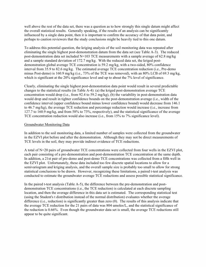
well above the rest of the data set, there was a question as to how strongly this single datum might affect the overall statistical results. Generally speaking, if the results of an analysis can be significantly influenced by a single data point, then it is important to confirm the accuracy of that data point, and perhaps to caution reviewers that the study conclusions might be heavily tied to this one datum.

To address this potential question, the kriging analysis of the soil monitoring data was repeated after eliminating the single highest post-demonstration datum from the data set (see Table A-3). The reduced post-demonstration data set included N=103 TCE measurements with a sample average of 62.8 mg/kg and a sample standard deviation of 172.7 mg/kg. With the reduced data set, the kriged post-demonstration global average TCE concentration is 59.2 mg/kg, with a two-sided, 80% confidence interval from 35.9 to 82.6 mg/kg. The estimated average TCE concentration reduction (i.e., Pre-demo minus Post-demo) is 160.9 mg/kg (i.e., 73% of the TCE was removed), with an 80% LCB of 69.3 mg/kg, which is significant at the 20% significance level and up to about the 7% level of significance.

Clearly, eliminating the single highest post-demonstration data point would result in several predictable changes to the statistical results (in Table A-4): (a) the kriged post-demonstration average TCE concentration would drop (i.e., from 92.4 to 59.2 mg/kg), (b) the variability in post-demonstration data would drop and result in tighter confidence bounds on the post-demonstration average (i.e., width of the confidence interval (upper confidence bound minus lower confidence bound) would decrease from 146.1 to 46.7 mg/kg), the average TCE reduction and percentage reduction would increase (i.e., increase from 127.7 to 160.9 mg/kg, and from 58% to 73%, respectively), and the statistical significance of the average TCE concentration reduction would also increase (i.e., from 15% to 7% significance level).

Groundwater Monitoring Data

In addition to the soil monitoring data, a limited number of samples were collected from the groundwater in the EZVI plot before and after the demonstration. Although they may not be direct measurements of TCE levels in the soil, they may provide indirect evidence of TCE reductions.

A total of N=20 pairs of groundwater TCE concentrations were collected from four wells in the EZVI plot, each pair consisting of a pre-demonstration and post-demonstration TCE concentration at the same depth. In addition, a 21st pair of pre-demo and post-demo TCE concentrations was collected from a fifth well in the EZVI plot. Unfortunately, these data included too few discrete spatial locations to allow for a semivariogram and kriging analysis, and the overall sample size is probably too small to allow for strong statistical conclusions to be drawn. However, recognizing these limitations, a paired t-test analysis was conducted to estimate the groundwater average TCE reductions and assess possible statistical significance.

In the paired t-test analysis (Table A-5), the difference between the pre-demonstration and post-demonstration TCE concentrations (i.e., the TCE reduction) is calculated at each discrete sampling location, and then the average difference in this data set is estimated. The corresponding statistical test (using the Student's t distribution instead of the normal distribution) evaluates whether the average difference (i.e., reduction) is significantly greater than zero (0). The results of this analysis indicate that the average TCE reduction for the 21 pairs of data was 804 umoles/L, and the statistical significance of the reduction is 0.66%. Even though the groundwater data set is small, the average TCE reductions still appear to be quite significant.

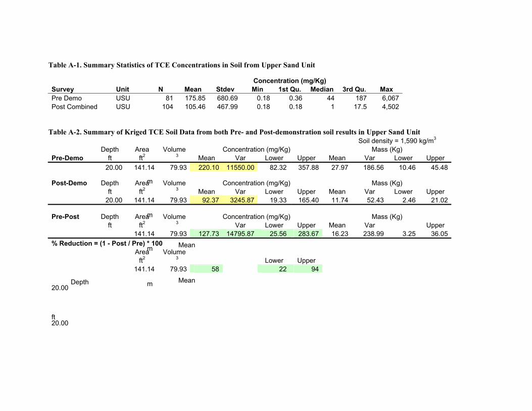
Table A-1. Summary Statistics of TCE Concentrations in Soil from Upper Sand Unit

Concentration (mg/Kg) Survey Unit N Mean Stdev Min 1st Qu. Median 3rd Qu. Max Pre Demo USU 81 175.85 680.69 0.18 0.36 44 187 6,067 Post Combined USU 104 105.46 467.99 0.18 0.18 1 17.5 4,502

Table A-2. Summary of Kriged TCE Soil Data from both Pre- and Post-demonstration soil results in Upper Sand Unit Soil density = 1,590 kg/m3

Depth Area Volume Concentration (mg/Kg) Mass (Kg) 3Pre-Demo ft ft2 Mean Var Lower Upper Mean Var Lower Upper

20.00 141.14 79.93 220.10 11550.00 82.32 357.88 27.97 186.56 10.46 45.48

Post-Demo Depth ft

20.00

mArea ft2

141.14

Volume 3

79.93 Mean

92.37

Concentration (mg/Kg) Var Lower

3245.87 19.33 Upper 165.40

Mean 11.74

Mass (Kg)Var Lower 52.43 2.46

Upper 21.02

Pre-Post Depth ft

mArea ft2

141.14

Volume 3

79.93 127.73

Concentration (mg/Kg) Var Lower

14795.87 25.56 Upper 283.67

Mean 16.23

Mass (Kg) Var 238.99 3.25

Upper 36.05

% Reduction = (1 - Post / Pre) * 100 mArea

ft2

141.14

Mean Volume

3

79.93 58 Lower

22 Upper

94

Depth m20.00 Mean

ft 20.00

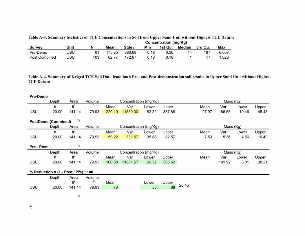
Pre-Demo Depth Area Volume Concentration (mg/Kg) Mass (Kg)

ft ft2

USU 20.00 141.14

3

79.93 Mean 220.10

Var Lower 11550.00 82.32

Upper 357.88

Mean 27.97

Var Lower 186.56 10.46

Upper 45.48

mPostDemo (Combined) Depth Area Volume Concentration (mg/Kg) Mass (Kg)

USU ft

20.00 ft2

141.14

3

79.93 Mean

59.22 Var 331.57

Lower 35.88

Upper 82.57

Mean 7.53

Var 5.36

Lower 4.56

Upper 10.49

Pre - Post m

Depth Area Volume 3 ft ft2

USU 20.00 141.14 79.93 Mean 160.88

Concentration (mg/Kg) Var Lower

11881.57 69.32 Upper 300.62

Mean Mass (Kg)

Var Lower 191.92 8.81

Upper 38.21

m% Reduction = (1 - Post / Pre) * 100

USU

Depth

20.00

Area ft2

141.14

Volume 3

79.93 Mean

73 Lower

55 Upper

88 20.45

m

ft

Table A-3. Summary Statistics of TCE Concentrations in Soil from Upper Sand Unit without Highest TCE Datum Concentration (mg/Kg)

Survey Unit N Mean Stdev Min 1st Qu. Median 3rd Qu. Max Pre-Demo USU 81 175.85 680.69 0.18 0.36 44 187 6,067 Post Combined USU 103 62.77 172.67 0.18 0.18 1 17 1,023

Table A-4. Summary of Kriged TCE Soil Data from both Pre- and Post-demonstration soil results in Upper Sand Unit without Highest TCE Datum

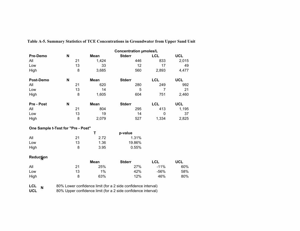
Table A-5. Summary Statistics of TCE Concentrations in Groundwater from Upper Sand Unit

Concentration µmoles/L Pre-Demo N Mean Stderr LCL UCL All 21 1,424 446 833 2,015 Low 13 33 12 17 49 High 8 3,685 560 2,893 4,477

Post-Demo N Mean Stderr LCL UCL All 21 620 280 249 992 Low 13 14 5 7 21 High 8 1,605 604 751 2,460

Pre - Post N Mean Stderr LCL UCL All 21 804 295 413 1,195 Low 13 19 14 0 37 High 8 2,079 527 1,334 2,825

One Sample t-Test for "Pre - Post" T p-value

All 21 2.72 1.31% Low 13 1.36 19.86% High 8 3.95 0.55%

Reduction N Mean Stderr LCL UCL

All 21 25% 27% -11% 60% Low 13 1% 42% -56% 58% High 8 63% 12% 46% 80%

LCL 80% Lower confidence limit (for a 2 side confidence interval) N UCL 80% Upper confidence limit (for a 2 side confidence interval)

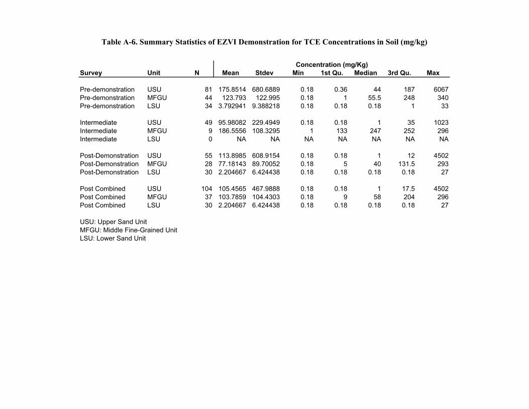
Table A-6. Summary Statistics of EZVI Demonstration for TCE Concentrations in Soil (mg/kg)

Concentration (mg/Kg) Survey Unit N Mean Stdev Min 1st Qu. Median 3rd Qu. Max

Pre-demonstration USU 81 175.8514 680.6889 0.18 0.36 44 187 6067 Pre-demonstration MFGU 44 123.793 122.995 0.18 1 55.5 248 340 Pre-demonstration LSU 34 3.792941 9.388218 0.18 0.18 0.18 1 33

Intermediate USU 49 95.98082 229.4949 0.18 0.18 1 35 1023 Intermediate MFGU 9 186.5556 108.3295 1 133 247 252 296 Intermediate LSU 0 NA NA NA NA NA NA NA

Post-Demonstration USU 55 113.8985 608.9154 0.18 0.18 1 12 4502 Post-Demonstration MFGU 28 77.18143 89.70052 0.18 5 40 131.5 293 Post-Demonstration LSU 30 2.204667 6.424438 0.18 0.18 0.18 0.18 27

Post Combined USU 104 105.4565 467.9888 0.18 0.18 1 17.5 4502 Post Combined MFGU 37 103.7859 104.4303 0.18 9 58 204 296 Post Combined LSU 30 2.204667 6.424438 0.18 0.18 0.18 0.18 27

USU: Upper Sand Unit MFGU: Middle Fine-Grained Unit LSU: Lower Sand Unit

A.2 Sample Collection and Extraction Methods

This section describes the modification made to the EPA standard methods to address the lithologic heterogeneities and extreme variability of the contaminant distribution expected in the DNAPL source region at Launch Complex 34. Horizontal variability was addressed by collecting a statistically determined number of soil cores in the EZVI Plot. The vertical variability at each soil coring location was addressed with this modified sampling and extraction procedure, which involved extraction of much larger quantities of soil in each extracted sample, as well as allowed collection and extraction of samples in the field per event. This extraction allowed the extraction and analysis of the entire vertical column of soil at a given coring location.

A.2.1 Soil Sample Collection (Modified ASTM D4547-91) (1997a)

The soil samples collected before and after the demonstration were sampled using a stainless steel sleeve driven into the subsurface by a Vibra-push LD-2 rig. After the sleeve had been driven the required distance, it was brought to the surface and the soil sample was examined and characterized for lithology. One quarter of the sample was sliced from the core and placed into a pre-weighed 500-mL polyethylene container containing methanol. At locations where a field duplicate sample was collected, a second one-quarter sample was split from the core and placed into another pre-weighed 500-mL polyethylene container containing methanol. The remaining portion of the core was placed into a 55-gallon drum and disposed of as waste. The samples were labeled with the date, time, and sample identification code, and stored on ice at 4°C until they were brought inside to the on-site laboratory for the extraction procedure.

After receiving the samples from the drilling activities, personnel staffing the field laboratory performed the methanol extraction procedure as outlined in Section A.2.2 of this appendix. The amount of methanol used to perform the extraction technique was 250 mL. The extraction procedure was performed on all of the primary samples collected during drilling activities and on 5% of the field duplicate samples collected for quality assurance. Samples were stored at 4°C until extraction procedures were performed. After the extraction procedure was finished, the soil samples were dried in an oven at 105°C and the dry weight of each sample was determined. The samples were then disposed of as waste. The remaining three-quarter section of each core previously stored in a separate 500-mL polyethylene bottle were archived until the off-site laboratory had completed the analysis of the methanol extract. The samples were then disposed of in an appropriate manner.

A.2.2 Soil Extraction Procedure (Modified EPA SW846-Method 5035)

After the soil samples were collected from the drilling operations, samples were placed in pre-labeled and pre-weighed 500-mL polyethylene containers with methanol and then stored in a refrigerator at 4°C until the extraction procedure was performed. Extraction procedures were performed on all of the “A” samples from the outdoor and indoor soil sampling. Extraction procedures also were performed on 5% of the duplicate (or “B”) samples to provide adequate quality assurance/quality control (QA/QC) on the extraction technique.

Extreme care was taken to minimize the disturbance of the soil sample so that loss of volatile components was minimal. Nitrile gloves were worn by field personnel whenever handling sample cores or pre-weighed sample containers. A modification of EPA SW846-Method 5035 was used to procure the cored samples in the field. Method 5035 lists different procedures for processing samples that are expected to contain low concentrations (0.5 to 200 µg/kg) or high concentrations

(>200 µg/kg) of volatile organic compounds (VOCs). Procedures for high levels of VOCs were used in the field because those procedures facilitated the processing of large-volume sample cores collected during soil sampling activities.

Two sample collection options and corresponding sample purging procedures are described in Method 5035; however, the procedure chosen for this study was based on collecting approximately 150 to 200 g of wet soil sample in a pre-weighed bottle that contains 250 mL of methanol. A modification of this method was used in the study, as described by the following procedure:

� The 150 to 200 g wet soil sample was collected and placed in a pre-weighed 500 mL polypropylene bottle filled with 250 mL of methanol. After capping, the bottle was reweighed to determine the total weight of the soil and the bottle with methanol. The bottle was marked with the location and the depth at which the sample was collected.

� After the containers were filled with methanol and the soil sample they were placed on an orbital shaker table and agitated for approximately 30 min.

� Containers were removed from the shaker table and reweighed to ensure that no methanol was lost during the agitation period. The containers were then placed upright and suspended soil matter was allowed to settle for approximately 15 min.

� The 500 mL containers were then placed in a floor-mounted centrifuge. The centrifuge speed was set at 3,000 rpm and the samples were centrifuged for 10 min.

� Methanol extract was then decanted into disposable 20-mL glass volatile organic analysis (VOA) vials using 10-mL disposable pipettes. The 20-mL glass VOA vials containing the extract then were capped, labeled, and stored in a refrigerator at 4°C until they were shipped on ice to the analytical laboratory.

� Methanol samples in VOA vials were placed in ice chests and maintained at approximately 4°C with ice. Samples were then shipped with properly completed chain-of-custody forms and custody seals to the subcontracted off-site laboratory.

� The dry weight of each of the soil samples was determined gravimetrically after decanting the remaining solvent and drying the soil in an oven at 105°C. Final concentrations of VOCs were calculated per the dry weight of soil.

Three potential concerns existed with the modified solvent extraction method. The first concern was that the United States Environmental Protection Agency (U.S. EPA) had not formally evaluated the use of methanol as a preservative for VOCs. However, methanol extraction often is used in site characterization studies including three technology demonstrations at Launch Complex 34 under U.S. EPA Superfund Innovative Technology Evaluation (SITE) program, so the uncertainty in using this approach was reasonable. The second concern was that the extraction procedure itself would introduce a significant dilution factor that could raise the method quantitation limit beyond that of a direct purge-and-trap procedure. The third concern was that excess methanol used in the extractions would likely fail the ignitability characteristic, thereby making the unused sample volume a hazardous waste. During characterization activities, the used methanol extract was disposed of as hazardous waste into a 55-gallon drum. This methanol extraction method was tested during preliminary site characterization activities at this site (see Appendix G, Table G-1) and, after a few refinements, was found to perform acceptably

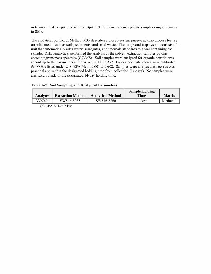
in terms of matrix spike recoveries. Spiked TCE recoveries in replicate samples ranged from 72 to 86%.

The analytical portion of Method 5035 describes a closed-system purge-and-trap process for use on solid media such as soils, sediments, and solid waste. The purge-and-trap system consists of a unit that automatically adds water, surrogates, and internals standards to a vial containing the sample. DHL Analytical performed the analysis of the solvent extraction samples by Gas chromatogram/mass spectrum (GC/MS). Soil samples were analyzed for organic constituents according to the parameters summarized in Table A-7. Laboratory instruments were calibrated for VOCs listed under U.S. EPA Method 601 and 602. Samples were analyzed as soon as was practical and within the designated holding time from collection (14 days). No samples were analyzed outside of the designated 14-day holding time.

Table A-7. Soil Sampling and Analytical Parameters

Analytes Extraction Method Analytical Method Sample Holding

Time Matrix VOCs(a) SW846-5035 SW846-8260 14 days Methanol

(a) EPA 601/602 list.

A.3 List of Standard Sample Collection and Analytical Methods

Table A-8. Sample Collection Procedures

Measurements Task/Sample

Collection Method Equipment Used Primary Objectives

CVOCs Soil sampling/ Mod.(a) ASTM D4547-98 (1997a)

Butyrate or acetate sleeves 500-mL plastic bottle

CVOCs Groundwater sampling/ Mod.(a) ASTM D4448-01 (1997b)

Peristaltic pump Teflon™ tubing

DHG(b) Groundwater sampling/ Mod.(a) ASTM D4448-01 (1997b)

Peristaltic pump Teflon™ tubing

Secondary Objectives Field parameters(c)

Inorganics–cations Inorganics–anions TOC, BOD, TDS, dissolved silica Alkalinity

Groundwater sampling/ Mod.(a) ASTM D4448-01 (1997b)

Peristaltic pump Teflon™ tubing

Hydraulic conductivity Hydraulic conductivity/ ASTM D4044-96 (1997c)

Winsitu® data logger Laptop computer

Groundwater level Water levels Water level indicator (a) Modifications to ASTM.

ASTM = American Society for Testing and Materials. American Society for Testing and Materials. 1997a. Standard Practice for Waste and Soils for Volatile Organics. Designation: D 4547-98. American Society for Testing and Materials. 1997b. Standard Guide for Sampling Groundwater Monitoring Wells. Designation: D 4448-01. American Society for Testing and Materials. 1997c. Standard Test Method (Field Procedure) for Instantaneous Change in Head (Slug) Tests for Determining Hydraulic Properties of Aquifers. Designation: D 4044-96.

(b) DHG: methane, ethene, and ethane (see Appendix D). (c) Field parameters include pH, ORP, temperature, DO, and conductivity. A flow-through cell will be

attached to the peristaltic pump when measuring field parameters.

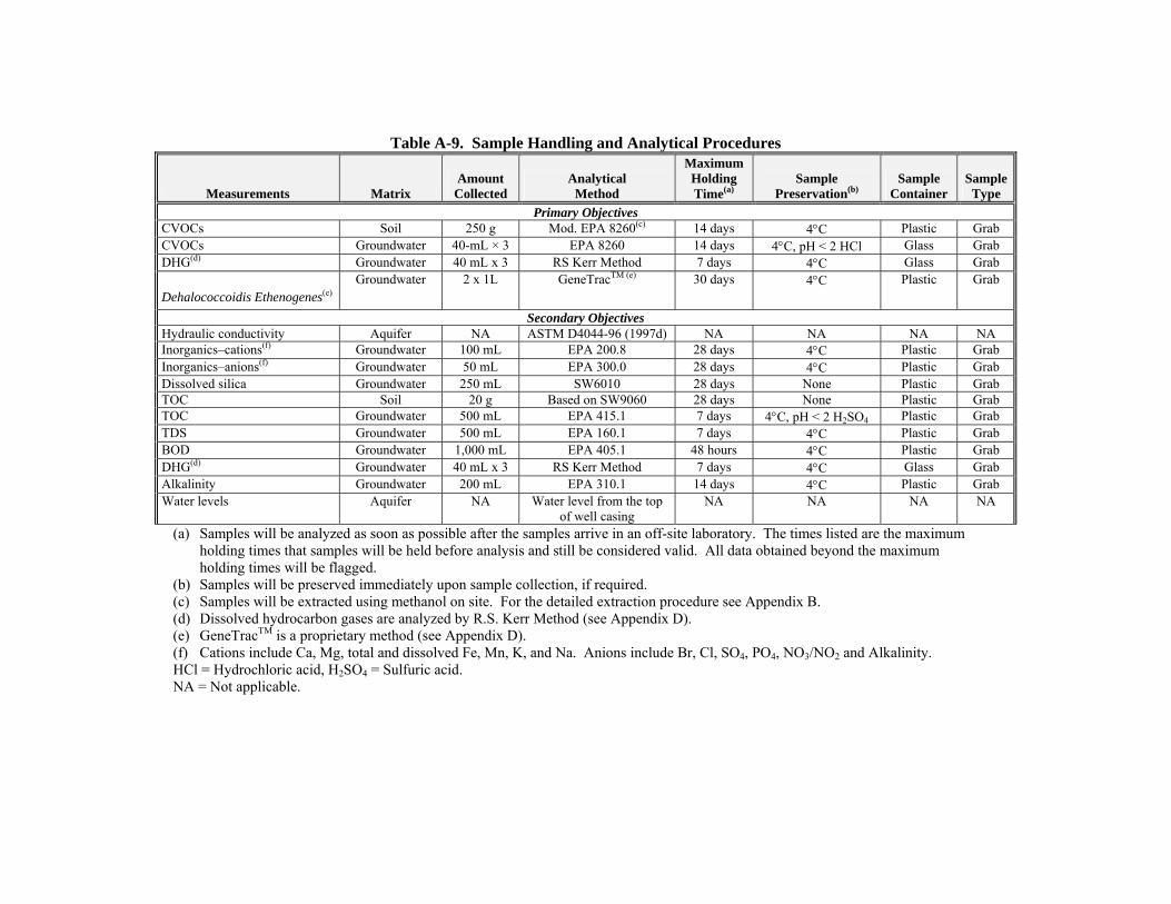
Table A-9. Sample Handling and Analytical Procedures

Measurements Matrix Amount

Collected Analytical

Method

Maximum Holding Time(a)

Sample Preservation(b)

Sample Container

Sample Type

Primary Objectives CVOCs Soil 250 g Mod. EPA 8260(c) 14 days 4°C Plastic Grab CVOCs Groundwater 40-mL × 3 EPA 8260 14 days 4°C, pH < 2 HCl Glass Grab DHG(d) Groundwater 40 mL x 3 RS Kerr Method 7 days 4°C Glass Grab

Dehalococcoidis Ethenogenes(e) Groundwater 2 x 1L GeneTracTM (e) 30 days 4°C Plastic Grab

Secondary Objectives Hydraulic conductivity Aquifer NA ASTM D4044-96 (1997d) NA NA NA NA Inorganics–cations(f) Groundwater 100 mL EPA 200.8 28 days 4°C Plastic Grab Inorganics–anions(f) Groundwater 50 mL EPA 300.0 28 days 4°C Plastic Grab Dissolved silica Groundwater 250 mL SW6010 28 days None Plastic Grab TOC Soil 20 g Based on SW9060 28 days None Plastic Grab TOC Groundwater 500 mL EPA 415.1 7 days 4°C, pH < 2 H2SO4 Plastic Grab TDS Groundwater 500 mL EPA 160.1 7 days 4°C Plastic Grab BOD Groundwater 1,000 mL EPA 405.1 48 hours 4°C Plastic Grab DHG(d) Groundwater 40 mL x 3 RS Kerr Method 7 days 4°C Glass Grab Alkalinity Groundwater 200 mL EPA 310.1 14 days 4°C Plastic Grab Water levels Aquifer NA Water level from the top

of well casing NA NA NA NA

(a) Samples will be analyzed as soon as possible after the samples arrive in an off-site laboratory. The times listed are the maximum holding times that samples will be held before analysis and still be considered valid. All data obtained beyond the maximum holding times will be flagged.

(b) Samples will be preserved immediately upon sample collection, if required. (c) Samples will be extracted using methanol on site. For the detailed extraction procedure see Appendix B. (d) Dissolved hydrocarbon gases are analyzed by R.S. Kerr Method (see Appendix D). (e) GeneTracTM is a proprietary method (see Appendix D). (f) Cations include Ca, Mg, total and dissolved Fe, Mn, K, and Na. Anions include Br, Cl, SO4, PO4, NO3/NO2 and Alkalinity. HCl = Hydrochloric acid, H2SO4 = Sulfuric acid. NA = Not applicable.

Appendix B

Hydrogeologic Measurements

B.1 Performance Monitoring Slug Tests B.2 Well Completion Diagrams B.3 Soil Coring Logsheets

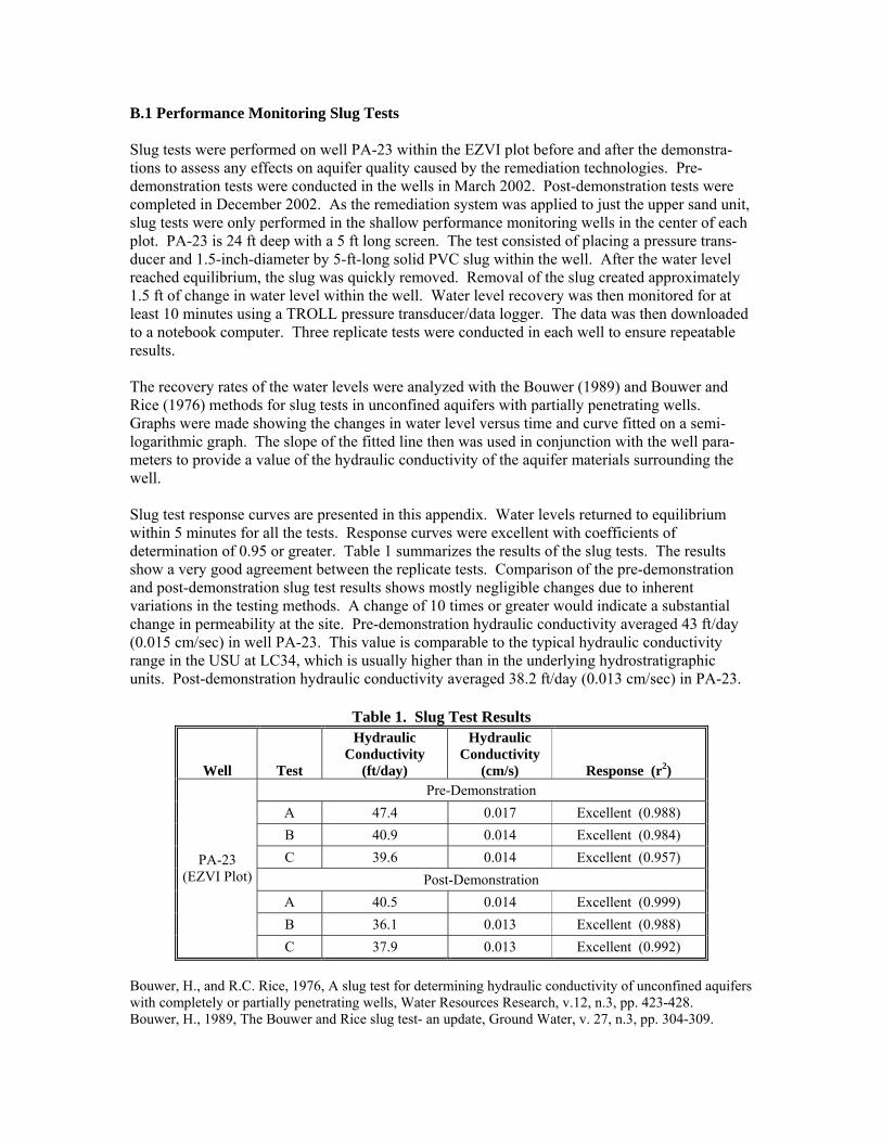
B.1 Performance Monitoring Slug Tests

Slug tests were performed on well PA-23 within the EZVI plot before and after the demonstra-tions to assess any effects on aquifer quality caused by the remediation technologies. Pre-demonstration tests were conducted in the wells in March 2002. Post-demonstration tests were completed in December 2002. As the remediation system was applied to just the upper sand unit, slug tests were only performed in the shallow performance monitoring wells in the center of each plot. PA-23 is 24 ft deep with a 5 ft long screen. The test consisted of placing a pressure trans-ducer and 1.5-inch-diameter by 5-ft-long solid PVC slug within the well. After the water level reached equilibrium, the slug was quickly removed. Removal of the slug created approximately 1.5 ft of change in water level within the well. Water level recovery was then monitored for at least 10 minutes using a TROLL pressure transducer/data logger. The data was then downloaded to a notebook computer. Three replicate tests were conducted in each well to ensure repeatable results.

The recovery rates of the water levels were analyzed with the Bouwer (1989) and Bouwer and Rice (1976) methods for slug tests in unconfined aquifers with partially penetrating wells. Graphs were made showing the changes in water level versus time and curve fitted on a semi-logarithmic graph. The slope of the fitted line then was used in conjunction with the well para-meters to provide a value of the hydraulic conductivity of the aquifer materials surrounding the well.

Slug test response curves are presented in this appendix. Water levels returned to equilibrium within 5 minutes for all the tests. Response curves were excellent with coefficients of determination of 0.95 or greater. Table 1 summarizes the results of the slug tests. The results show a very good agreement between the replicate tests. Comparison of the pre-demonstration and post-demonstration slug test results shows mostly negligible changes due to inherent variations in the testing methods. A change of 10 times or greater would indicate a substantial change in permeability at the site. Pre-demonstration hydraulic conductivity averaged 43 ft/day (0.015 cm/sec) in well PA-23. This value is comparable to the typical hydraulic conductivity range in the USU at LC34, which is usually higher than in the underlying hydrostratigraphic units. Post-demonstration hydraulic conductivity averaged 38.2 ft/day (0.013 cm/sec) in PA-23.

Table 1. Slug Test Results

Well Test

Hydraulic Conductivity

(ft/day)

Hydraulic Conductivity

(cm/s) Response (r2) Pre-Demonstration

A 47.4 0.017 Excellent (0.988) B 40.9 0.014 Excellent (0.984)

PA-23 C 39.6 0.014 Excellent (0.957) (EZVI Plot) Post-Demonstration

A 40.5 0.014 Excellent (0.999) B 36.1 0.013 Excellent (0.988) C 37.9 0.013 Excellent (0.992)

Bouwer, H., and R.C. Rice, 1976, A slug test for determining hydraulic conductivity of unconfined aquifers with completely or partially penetrating wells, Water Resources Research, v.12, n.3, pp. 423-428. Bouwer, H., 1989, The Bouwer and Rice slug test- an update, Ground Water, v. 27, n.3, pp. 304-309.

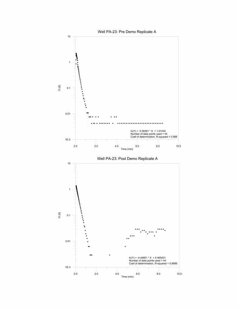
Well PA-23: Pre Demo Replicate A

0.0 2.0 4.0 6.0 8.0 10.0 Time (min)

Well PA-23: Post Demo Replicate A

0.0 2.0 4.0 6.0 8.0 10.0 Time (min)

1E-3

0.01

0.1

1

10

Yt (f

t)

ln(Y) = -5.38361 * X + 1.01034 Number of data points used = 44 Coef of determination, R-squared = 0.988

1E-3

0.01

0.1

1

10

Yt (f

t)

ln(Y) = -4.44801 * X + 0.465421 Number of data points used = 44 Coef of determination, R-squared = 0.9995

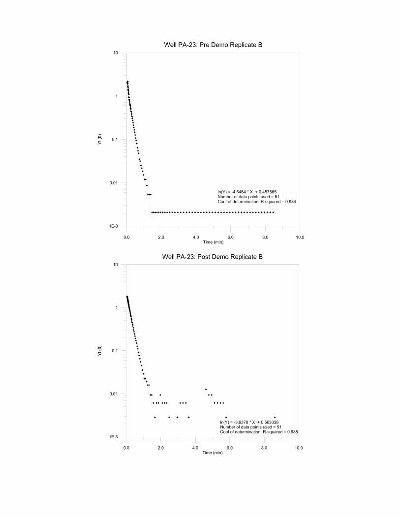
Well PA-23: Pre Demo Replicate B

0.0 2.0 4.0 6.0 8.0 10.0 Time (min)

Well PA-23: Post Demo Replicate B

0.0 2.0 4.0 6.0 8.0 10.0 Time (min)

1E-3

0.01

0.1

1

10

Yt (f

t)

ln(Y) = -4.6464 * X + 0.457565 Number of data points used = 51 Coef of determination, R-squared = 0.984

1E-3

0.01

0.1

1

10

Yt (f

t)

ln(Y) = -3.9378 * X + 0.563338 Number of data points used = 51 Coef of determination, R-squared = 0.988

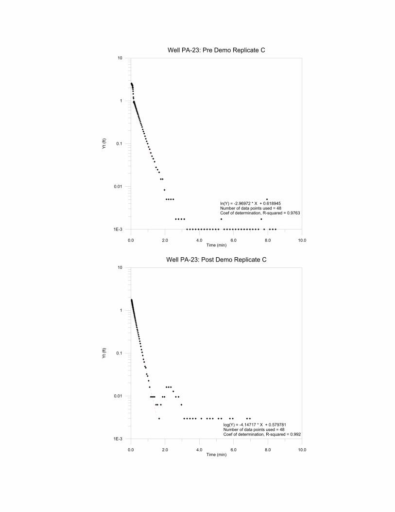
Well PA-23: Pre Demo Replicate C

0.0 2.0 4.0 6.0 8.0 10.0 Time (min)

Well PA-23: Post Demo Replicate C

0.0 2.0 4.0 6.0 8.0 10.0 Time (min)

1E-3

0.01

0.1

1

10

Yt (f

t)

ln(Y) = -2.96972 * X + 0.618945 Number of data points used = 48 Coef of determination, R-squared = 0.9763

1E-3

0.01

0.1

1

10

Yt (f

t)

log(Y) = -4.14717 * X + 0.579781 Number of data points used = 48 Coef of determination, R-squared = 0.992

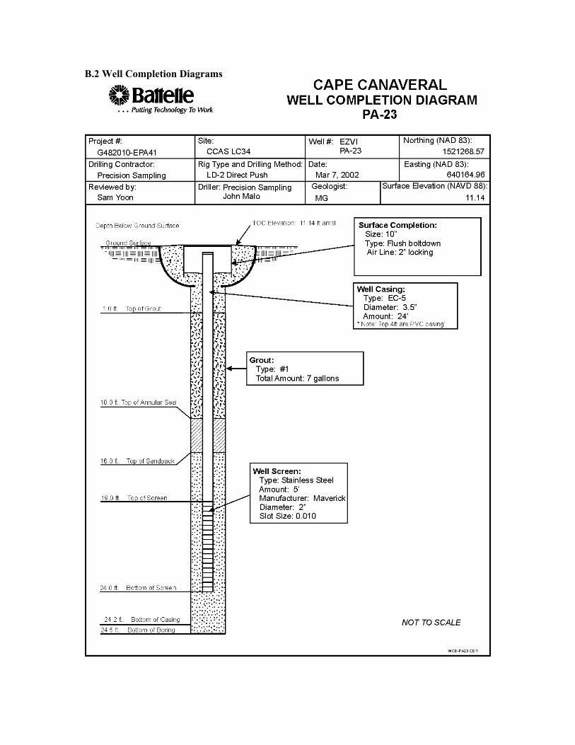
B.2 Well Completion Diagrams

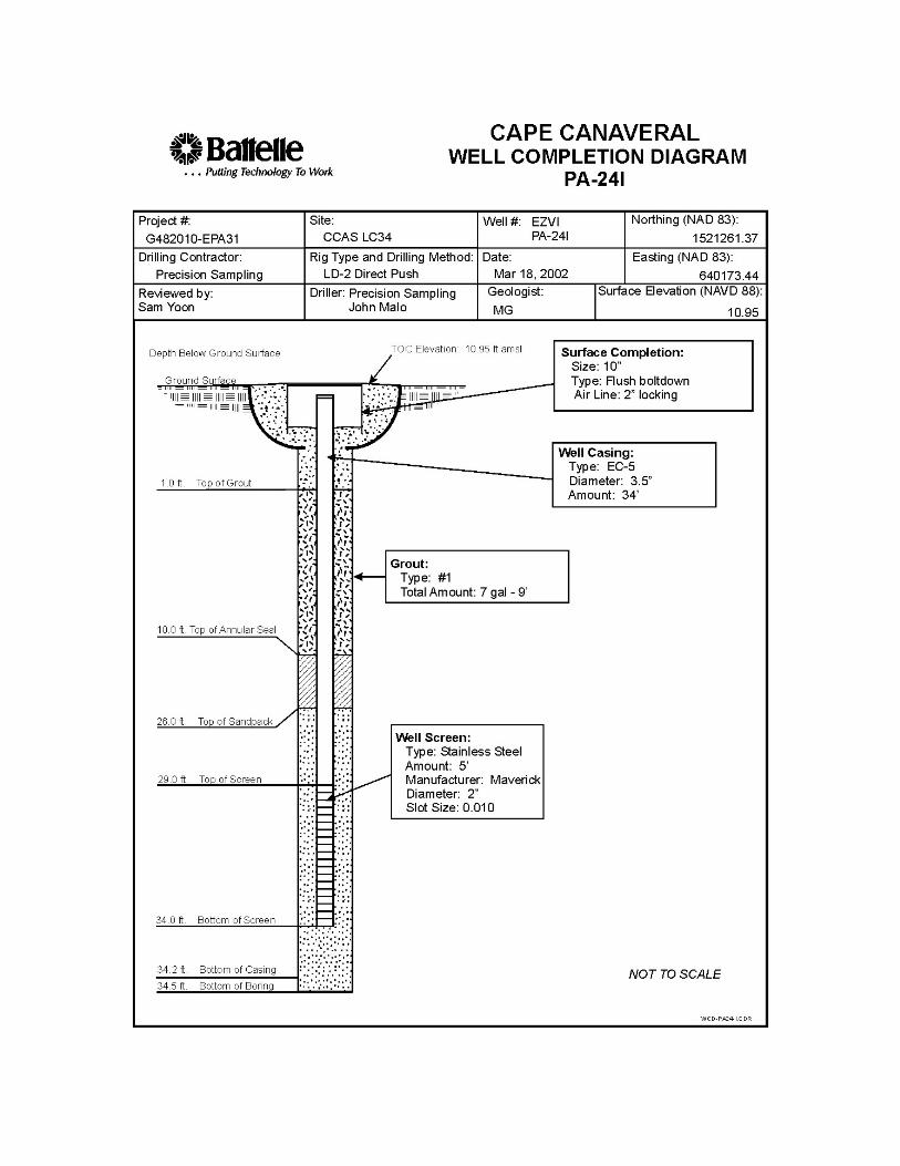
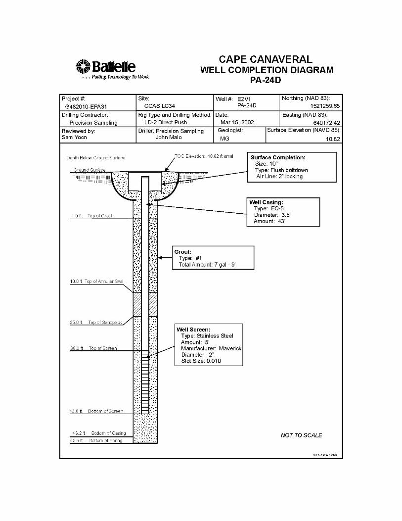
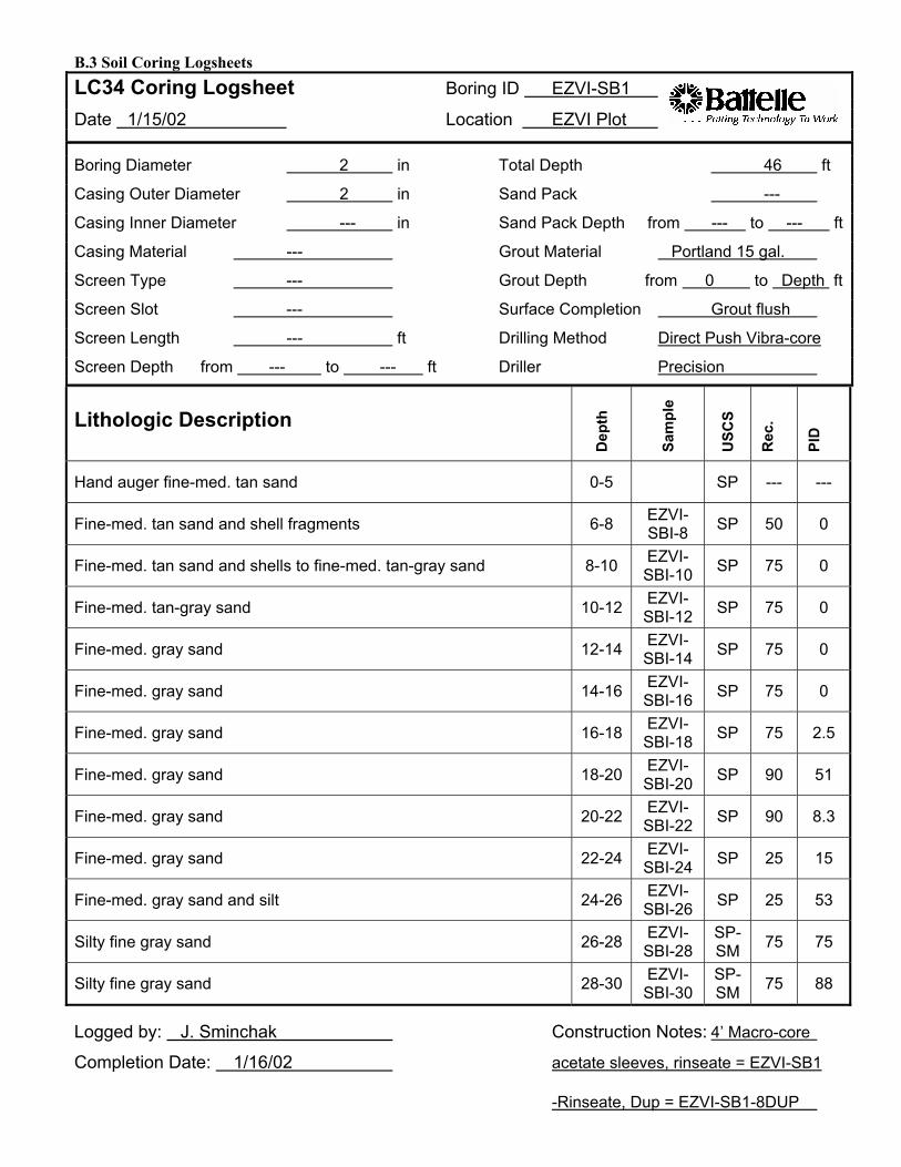
LC34 Coring Logsheet Date 1/15/02

Boring ID

Location

EZVI-SB1

EZVI Plot

Boring Diameter 2 in Total Depth 46 ft

Casing Outer Diameter 2 in Sand Pack ---

Casing Inner Diameter --- in Sand Pack Depth from --- to --- ft

Casing Material --- Grout Material Portland 15 gal.

Screen Type --- Grout Depth from 0 to Depth ft

Screen Slot --- Surface Completion Grout flush

Screen Length --- ft Drilling Method Direct Push Vibra-core

Screen Depth from --- to --- ft Driller Precision

Lithologic Description

Dep

th

Sam

ple

USC

S

Rec

.

PID

Hand auger fine-med. tan sand 0-5 SP --- ---

Fine-med. tan sand and shell fragments 6-8 EZVI-SBI-8 SP 50 0

Fine-med. tan sand and shells to fine-med. tan-gray sand 8-10 EZVI-SBI-10 SP 75 0

Fine-med. tan-gray sand 10-12 EZVI-SBI-12 SP 75 0

Fine-med. gray sand 12-14 EZVI-SBI-14 SP 75 0

Fine-med. gray sand 14-16 EZVI-SBI-16 SP 75 0

Fine-med. gray sand 16-18 EZVI­SBI-18 SP 75 2.5

Fine-med. gray sand 18-20 EZVI-SBI-20 SP 90 51

Fine-med. gray sand 20-22 EZVI­SBI-22 SP 90 8.3

Fine-med. gray sand 22-24 EZVI-SBI-24 SP 25 15

Fine-med. gray sand and silt 24-26 EZVI-SBI-26 SP 25 53

Silty fine gray sand 26-28 EZVI­SBI-28

SP-SM 75 75

Silty fine gray sand 28-30 EZVI­SBI-30

SP-SM 75 88

Logged by: J. Sminchak Construction Notes: 4’ Macro-core

Completion Date: 1/16/02 acetate sleeves, rinseate = EZVI-SB1

-Rinseate, Dup = EZVI-SB1-8DUP

B.3 Soil Coring Logsheets

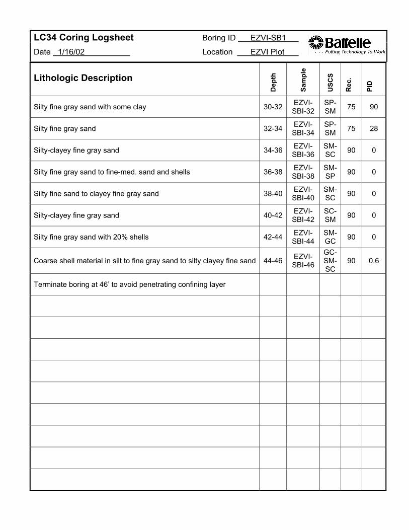
LC34 Coring Logsheet Boring ID EZVI-SB1

Date 1/16/02 Location EZVI Plot

Lithologic Description

Dep

th

Sam

ple

USC

S

Rec

.

PID

Silty fine gray sand with some clay 30-32 EZVI­SBI-32

SP­SM 75 90

Silty fine gray sand 32-34 EZVI­SBI-34

SP­SM 75 28

Silty-clayey fine gray sand 34-36 EZVI­SBI-36

SM­SC 90 0

Silty fine gray sand to fine-med. sand and shells 36-38 EZVI­SBI-38

SM­SP 90 0

Silty fine sand to clayey fine gray sand 38-40 EZVI­SBI-40

SM­SC 90 0

Silty-clayey fine gray sand 40-42 EZVI­SBI-42

SC­SM 90 0

Silty fine gray sand with 20% shells 42-44 EZVI­SBI-44

SM­GC 90 0

Coarse shell material in silt to fine gray sand to silty clayey fine sand 44-46 EZVI­SBI-46

GC­SM­SC

90 0.6

Terminate boring at 46’ to avoid penetrating confining layer

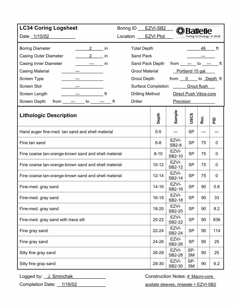
LC34 Coring Logsheet Date 1/15/02

Boring ID

Location

EZVI-SB2

EZVI Plot

Boring Diameter 2 in Total Depth 46 ft

Casing Outer Diameter 2 in Sand Pack ---

Casing Inner Diameter --- in Sand Pack Depth from --- to --- ft

Casing Material --- Grout Material Portland 15 gal.

Screen Type --- Grout Depth from 0 to Depth ft

Screen Slot --- Surface Completion Grout flush

Screen Length --- ft Drilling Method Direct Push Vibra-core

Screen Depth from --- to --- ft Driller Precision

Lithologic Description

Dep

th

Sam

ple

USC

S

Rec

.

PID

Hand auger fine-med. tan sand and shell material 0-5 --- SP --- ---

Fine tan sand 6-8 EZVI-SB2-8 SP 75 0

Fine coarse tan-orange-brown sand and shell material 8-10 EZVI-SB2-10 SP 75 0

Fine coarse tan-orange-brown sand and shell material 10-12 EZVI-SB2-12 SP 75 0

Fine coarse tan-orange-brown sand and shell material 12-14 EZVI-SB2-14 SP 75 0

Fine-med. gray sand 14-16 EZVI-SB2-16 SP 90 0.8

Fine-med. gray sand 16-18 EZVI-SB2-18 SP 90 33

Fine-med. gray sand 18-20 EZVI-SB2-20 SP 90 8.2

Fine-med. gray sand with trace silt 20-22 EZVI-SB2-22 SP 90 836

Fine gray sand 22-24 EZVI-SB2-24 SP 90 114

Fine gray sand 24-26 EZVI-SB2-26 SP 90 25

Silty fine gray sand 26-28 EZVI­SB2-28

SP-SM 90 25

Silty fine gray sand 28-30 EZVI­SB2-30

SP-SM 90 6.2

Logged by: J. Sminchak Construction Notes: 4’ Macro-core

Completion Date: 1/16/02 acetate sleeves, rinseate = EZVI-SB2

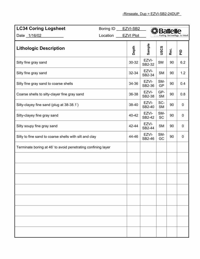
-Rinseate, Dup = EZVI-SB2-24DUP

LC34 Coring Logsheet Boring ID

Date 1/16/02 Location

EZVI-SB2

EZVI Plot

Lithologic Description

Dep

th

Sam

ple

USC

S

Rec

.

PID

Silty fine gray sand 30-32 EZVI­SB2-32 SM 90 6.2

Silty fine gray sand 32-34 EZVI­SB2-34 SM 90 1.2

Silty fine gray sand to coarse shells 34-36 EZVI­SB2-36

SM­GP 90 0.4

Coarse shells to silty-clayer fine gray sand 36-38 EZVI­SB2-38

GP­SM 90 0.8

Silty-clayey fine sand (plug at 38-38.1’) 38-40 EZVI­SB2-40

SC­SM 90 0

Silty-clayey fine gray sand 40-42 EZVI­SB2-42

SM­SC 90 0

Silty soupy fine gray sand 42-44 EZVI­SB2-44 SM 90 0

Silty to fine sand to coarse shells with silt and clay 44-46 EZVI­SB2-46

SM­GC 90 0

Terminate boring at 46’ to avoid penetrating confining layer

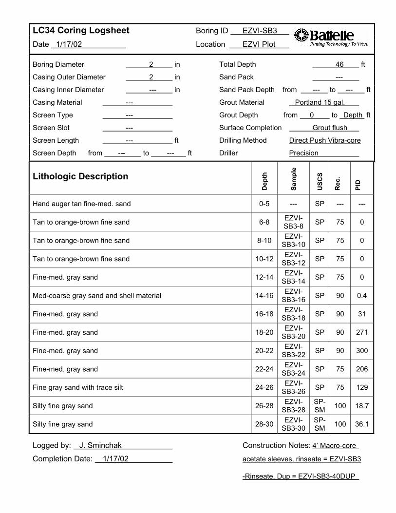
LC34 Coring Logsheet Date 1/17/02

Boring ID

Location

EZVI-SB3

EZVI Plot

Boring Diameter

Casing Outer Diameter

Casing Inner Diameter

Casing Material

Screen Type

Screen Slot

Screen Length

Screen Depth from

---

---

---

---

---

2

2

to

---

in

in

in

ft

--- ft

Total Depth 46 ft

Sand Pack ---

Sand Pack Depth from to ft

Grout Material Portland 15 gal.

Grout Depth from 0 to Depth ft

Surface Completion Grout flush

Drilling Method Direct Push Vibra-core

Driller Precision

--- ---

Lithologic Description

Dep

th

Sam

ple

USC

S

Rec

.

PID

Hand auger tan fine-med. sand 0-5 --- SP --- ---

Tan to orange-brown fine sand

Tan to orange-brown fine sand

Tan to orange-brown fine sand

Fine-med. gray sand

Med-coarse gray sand and shell material

Fine-med. gray sand

Fine-med. gray sand

Fine-med. gray sand

Fine-med. gray sand

Fine gray sand with trace silt

Silty fine gray sand

Silty fine gray sand

6-8

8-10

10-12

12-14

14-16

16-18

18-20

20-22

22-24

24-26

26-28

28-30

EZVI­SB3-8 EZVI­

SB3-10 EZVI­

SB3-12 EZVI­

SB3-14 EZVI­

SB3-16 EZVI­

SB3-18 EZVI­

SB3-20 EZVI­

SB3-22 EZVI­

SB3-24 EZVI­

SB3-26 EZVI­

SB3-28 EZVI­

SB3-30

SP

SP

SP

SP

SP

SP

SP

SP

SP

SP

SP­SM SP­SM

75

75

75

75

90

90

90

90

75

75

100

100

0

0

0

0

0.4

31

271

300

206

129

18.7

36.1

Logged by: J. Sminchak

Completion Date: 1/17/02

Construction Notes: 4’ Macro-core

acetate sleeves, rinseate = EZVI-SB3

-Rinseate, Dup = EZVI-SB3-40DUP

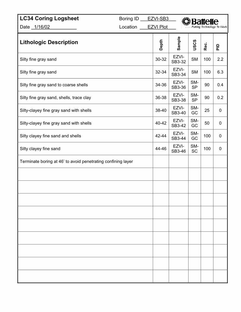
LC34 Coring Logsheet Boring ID

Date 1/16/02 Location

EZVI-SB3

EZVI Plot

Lithologic Description

Dep

th

Sam

ple

USC

S

Rec

.

PID

Silty fine gray sand 30-32 EZVI­SB3-32 SM 100 2.2

Silty fine gray sand 32-34 EZVI­SB3-34 SM 100 6.3

Silty fine gray sand to coarse shells 34-36 EZVI­SB3-36

SM­SP 90 0.4

Silty fine gray sand, shells, trace clay 36-38 EZVI­SB3-38

SM­SP 90 0.2

Silty-clayey fine gray sand with shells 38-40 EZVI­SB3-40

SM­GC 25 0

Silty-clayey fine gray sand with shells 40-42 EZVI­SB3-42

SM­GC 50 0

Silty clayey fine sand and shells 42-44 EZVI­SB3-44

SM­GC 100 0

Silty clayey fine sand 44-46 EZVI­SB3-46

SM­SC 100 0

Terminate boring at 46’ to avoid penetrating confining layer

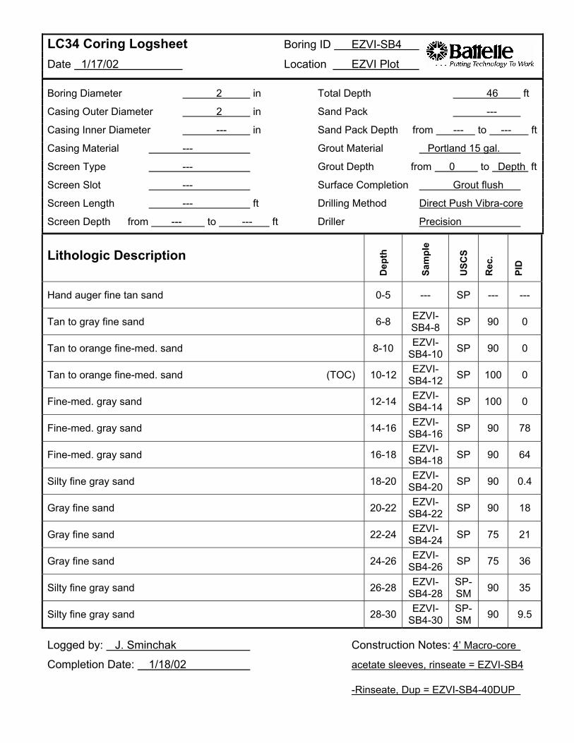
LC34 Coring Logsheet Date 1/17/02

Boring ID

Location

EZVI-SB4

EZVI Plot

Boring Diameter

Casing Outer Diameter

Casing Inner Diameter

Casing Material

Screen Type

Screen Slot

Screen Length

Screen Depth from

---

---

---

---

---

2

2

to

---

in

in

in

ft

--- ft

Total Depth 46 ft

Sand Pack ---

Sand Pack Depth from to ft

Grout Material Portland 15 gal.

Grout Depth from 0 to Depth ft

Surface Completion Grout flush

Drilling Method Direct Push Vibra-core

Driller Precision

--- ---

Lithologic Description

Dep

th

Sam

ple

USC

S

Rec

.

PID

Hand auger fine tan sand 0-5 --- SP --- ---

Tan to gray fine sand

Tan to orange fine-med. sand

Tan to orange fine-med. sand

Fine-med. gray sand

Fine-med. gray sand

Fine-med. gray sand

Silty fine gray sand

Gray fine sand

Gray fine sand

Gray fine sand

Silty fine gray sand

Silty fine gray sand

(TOC)

6-8

8-10

10-12

12-14

14-16

16-18

18-20

20-22

22-24

24-26

26-28

28-30

EZVI­SB4-8 EZVI­

SB4-10 EZVI­

SB4-12 EZVI­

SB4-14 EZVI­

SB4-16 EZVI­

SB4-18 EZVI­

SB4-20 EZVI­

SB4-22 EZVI­

SB4-24 EZVI­

SB4-26 EZVI­

SB4-28 EZVI­

SB4-30

SP

SP

SP

SP

SP

SP

SP

SP

SP

SP

SP­SM SP­SM

90

90

100

100

90

90

90

90

75

75

90

90

0

0

0

0

78

64

0.4

18

21

36

35

9.5

Logged by: J. Sminchak

Completion Date: 1/18/02

Construction Notes: 4’ Macro-core

acetate sleeves, rinseate = EZVI-SB4

-Rinseate, Dup = EZVI-SB4-40DUP

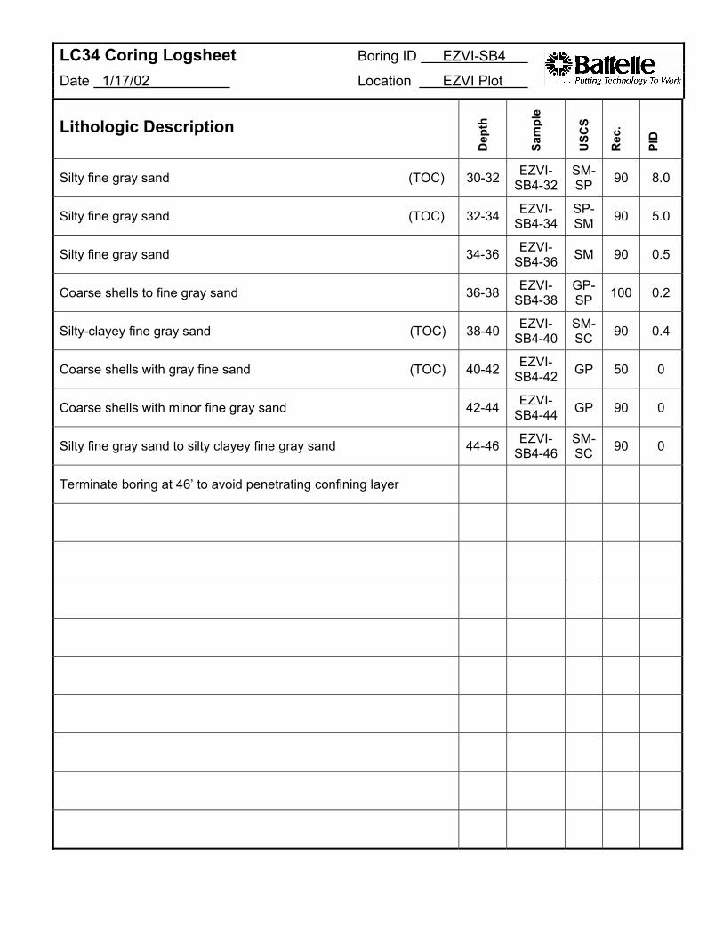
LC34 Coring Logsheet Boring ID EZVI-SB4

Date 1/17/02 Location EZVI Plot

Lithologic Description

Dep

th

Sam

ple

USC

S

Rec

.

PID

Silty fine gray sand (TOC) 30-32 EZVI­SB4-32

SM­SP 90 8.0

Silty fine gray sand (TOC) 32-34 EZVI­SB4-34

SP­SM 90 5.0

Silty fine gray sand 34-36 EZVI­SB4-36 SM 90 0.5

Coarse shells to fine gray sand 36-38 EZVI­SB4-38

GP­SP 100 0.2

Silty-clayey fine gray sand (TOC) 38-40 EZVI­SB4-40

SM­SC 90 0.4

Coarse shells with gray fine sand (TOC) 40-42 EZVI­SB4-42 GP 50 0

Coarse shells with minor fine gray sand 42-44 EZVI­SB4-44 GP 90 0

Silty fine gray sand to silty clayey fine gray sand 44-46 EZVI­SB4-46

SM­SC 90 0

Terminate boring at 46’ to avoid penetrating confining layer

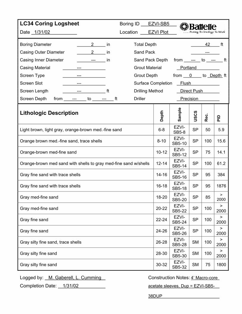
LC34 Coring Logsheet Date 1/31/02

Boring ID

Location

EZVI-SB5

EZVI Plot

Boring Diameter 2 in Total Depth 42 ft

Casing Outer Diameter 2 in Sand Pack ---

Casing Inner Diameter --- in Sand Pack Depth from --- to --- ft

Casing Material --- Grout Material Portland

Screen Type --- Grout Depth from 0 to Depth ft

Screen Slot --- Surface Completion Flush

Screen Length --- ft Drilling Method Direct Push

Screen Depth from --- to --- ft Driller Precision

Lithologic Description

Dep

th

Sam

ple

USC

S

Rec

.

PID

Light brown, light gray, orange-brown med.-fine sand 6-8 EZVI-SB5-8 SP 50 5.9

Orange brown med.-fine sand, trace shells 8-10 EZVI-SB5-10 SP 100 15.6

Orange-brown med-fine sand 10-12 EZVI-SB5-12 SP 75 14.1

Orange-brown med sand with shells to gray med-fine sand w/shells 12-14 EZVI-SB5-14 SP 100 61.2

Gray fine sand with trace shells 14-16 EZVI-SB5-16 SP 95 384

Gray fine sand with trace shells 16-18 EZVI-SB5-18 SP 95 1876

Gray med-fine sand 18-20 EZVI­SB5-20 SP 85 >

2000

Gray med-fine sand 20-22 EZVI­SB5-22 SP 100 >

2000

Gray fine sand 22-24 EZVI­SB5-24 SP 100 >

2000

Gray fine sand 24-26 EZVI­SB5-26 SP 100 >

2000

Gray silty fine sand, trace shells 26-28 EZVI­SB5-28 SM 100 >

2000

Gray silty fine sand 28-30 EZVI­SB5-30 SM 100 >

2000

Gray silty fine sand 30-32 EZVI-SB5-32 SM 75 1800

Logged by: M. Gaberell, L. Cumming Construction Notes: 4’ Macro-core

Completion Date: 1/31/02 acetate sleeves, Dup = EZVI-SB5-

38DUP

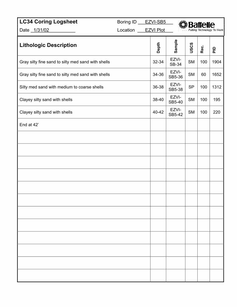
LC34 Coring Logsheet Boring ID

Date 1/31/02 Location

EZVI-SB5

EZVI Plot

Lithologic Description

Dep

th

Sam

ple

USC

S

Rec

.

PID

Gray silty fine sand to silty med sand with shells 32-34 EZVI­SB-34 SM 100 1904

Gray silty fine sand to silty med sand with shells 34-36 EZVI­SB5-36 SM 60 1652

Silty med sand with medium to coarse shells 36-38 EZVI­SB5-38 SP 100 1312

Clayey silty sand with shells 38-40 EZVI­SB5-40 SM 100 195

Clayey silty sand with shells 40-42 EZVI­SB5-42 SM 100 220

End at 42’

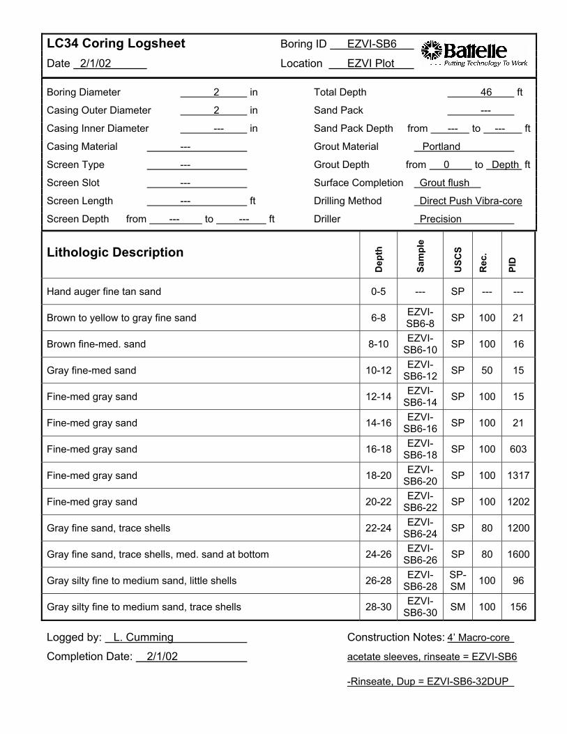
LC34 Coring Logsheet Date 2/1/02

Boring ID

Location

EZVI-SB6

EZVI Plot

Boring Diameter 2 in Total Depth 46 ft

Casing Outer Diameter 2 in Sand Pack ---

Casing Inner Diameter --- in Sand Pack Depth from --- to --- ft

Casing Material --- Grout Material Portland

Screen Type --- Grout Depth from 0 to Depth ft

Screen Slot --- Surface Completion Grout flush

Screen Length --- ft Drilling Method Direct Push Vibra-core

Screen Depth from --- to --- ft Driller Precision

Lithologic Description

Dep

th

Sam

ple

USC

S

Rec

.

PID

Hand auger fine tan sand 0-5 --- SP --- ---

Brown to yellow to gray fine sand 6-8 EZVI-SB6-8 SP 100 21

Brown fine-med. sand 8-10 EZVI-SB6-10 SP 100 16

Gray fine-med sand 10-12 EZVI-SB6-12 SP 50 15

Fine-med gray sand 12-14 EZVI-SB6-14 SP 100 15

Fine-med gray sand 14-16 EZVI-SB6-16 SP 100 21

Fine-med gray sand 16-18 EZVI-SB6-18 SP 100 603

Fine-med gray sand 18-20 EZVI-SB6-20 SP 100 1317

Fine-med gray sand 20-22 EZVI-SB6-22 SP 100 1202

Gray fine sand, trace shells 22-24 EZVI-SB6-24 SP 80 1200

Gray fine sand, trace shells, med. sand at bottom 24-26 EZVI-SB6-26 SP 80 1600

Gray silty fine to medium sand, little shells 26-28 EZVI­SB6-28

SP-SM 100 96

Gray silty fine to medium sand, trace shells 28-30 EZVI-SB6-30 SM 100 156

Logged by: L. Cumming Construction Notes: 4’ Macro-core

Completion Date: 2/1/02 acetate sleeves, rinseate = EZVI-SB6

-Rinseate, Dup = EZVI-SB6-32DUP

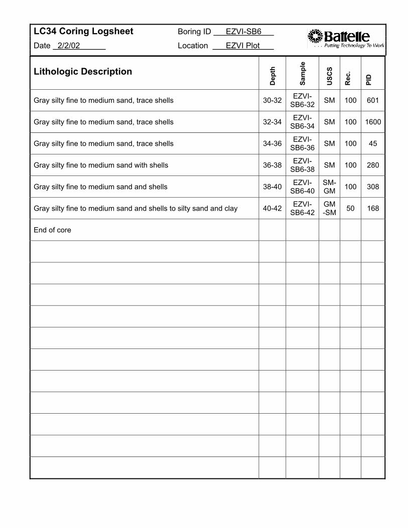
LC34 Coring Logsheet Boring ID EZVI-SB6

Date 2/2/02 Location EZVI Plot

Lithologic Description

Dep

th

Sam

ple

USC

S

Rec

.

PID

Gray silty fine to medium sand, trace shells 30-32 EZVI­SB6-32 SM 100 601

Gray silty fine to medium sand, trace shells 32-34 EZVI­SB6-34 SM 100 1600

Gray silty fine to medium sand, trace shells 34-36 EZVI­SB6-36 SM 100 45

Gray silty fine to medium sand with shells 36-38 EZVI­SB6-38 SM 100 280

Gray silty fine to medium sand and shells 38-40 EZVI­SB6-40

SM­GM 100 308

Gray silty fine to medium sand and shells to silty sand and clay 40-42 EZVI­SB6-42

GM -SM 50 168

End of core

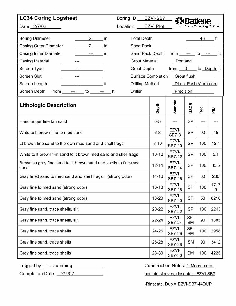
LC34 Coring Logsheet Date 2/7/02

Boring ID

Location

EZVI-SB7

EZVI Plot

Boring Diameter 2 in Total Depth 46 ft

Casing Outer Diameter 2 in Sand Pack ---

Casing Inner Diameter --- in Sand Pack Depth from --- to --- ft

Casing Material --- Grout Material Portland

Screen Type --- Grout Depth from 0 to Depth ft

Screen Slot --- Surface Completion Grout flush

Screen Length --- ft Drilling Method Direct Push Vibra-core

Screen Depth from --- to --- ft Driller Precision

Lithologic Description

Dep

th

Sam

ple

USC

S

Rec

.

PID

Hand auger fine tan sand 0-5 --- SP --- ---

Whte to lt brown fine to med sand 6-8 EZVI-SB7-8 SP 90 45

Lt brown fine sand to lt brown med sand and shell frags 8-10 EZVI-SB7-10 SP 100 12.4

White to lt brown f-m sand to lt brown med sand and shell frags 10-12 EZVI-SB7-12 SP 100 5.1

Brownish gray fine sand to lit brown sand and shells to fine-med sand 12-14 EZVI­

SB7-14 SP 100 35.5

Gray fined sand to med sand and shell frags (strong odor) 14-16 EZVI-SB7-16 SP 80 230

Gray fine to med sand (strong odor) 16-18 EZVI­SB7-18 SP 100 1717

5

Gray fine to med sand (strong odor) 18-20 EZVI-SB7-20 SP 50 8210

Gray fine sand, trace shells, silt 20-22 EZVI-SB7-22 SP 100 2243

Gray fine sand, trace shells, silt 22-24 EZVI­SB7-24

SP-SM 90 1885

Gray fine sand, trace shells 24-26 EZVI­SB7-26

SP-SM 100 2958

Gray fine sand, trace shells 26-28 EZVI-SB7-28 SM 90 3412

Gray fine sand, trace shells 28-30 EZVI-SB7-30 SM 100 4225

Logged by: L. Cumming Construction Notes: 4’ Macro-core

Completion Date: 2/7/02 acetate sleeves, rinseate = EZVI-SB7

-Rinseate, Dup = EZVI-SB7-44DUP

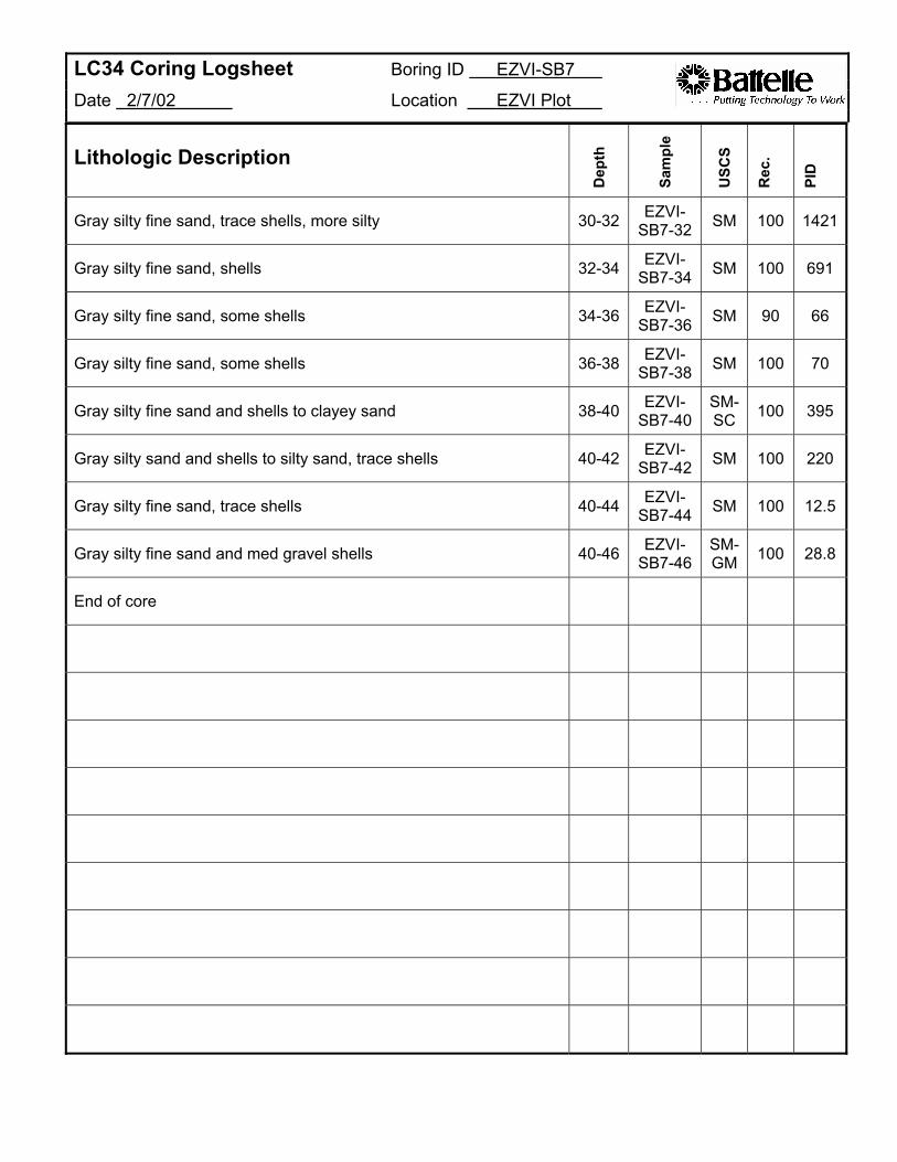
LC34 Coring Logsheet Boring ID

Date 2/7/02 Location

EZVI-SB7

EZVI Plot

Lithologic Description

Dep

th

Sam

ple

USC

S

Rec

.

PID

Gray silty fine sand, trace shells, more silty 30-32 EZVI­SB7-32 SM 100 1421

Gray silty fine sand, shells 32-34 EZVI­SB7-34 SM 100 691

Gray silty fine sand, some shells 34-36 EZVI­SB7-36 SM 90 66

Gray silty fine sand, some shells 36-38 EZVI­SB7-38 SM 100 70

Gray silty fine sand and shells to clayey sand 38-40 EZVI­SB7-40

SM­SC 100 395

Gray silty sand and shells to silty sand, trace shells 40-42 EZVI­SB7-42 SM 100 220

Gray silty fine sand, trace shells 40-44 EZVI­SB7-44 SM 100 12.5

Gray silty fine sand and med gravel shells 40-46 EZVI­SB7-46

SM­GM 100 28.8

End of core

LC34 Coring Logsheet Date 1/18/02

Boring ID EZVI-WP1

Location EZVI Plot

Boring Diameter

Casing Outer Diameter

Casing Inner Diameter

Casing Material

Screen Type ---

Screen Slot ---

Screen Length

Screen Depth from

---

---

---

2

2

to

---

in

in

in

ft

---

Total Depth 40 ft

Sand Pack ---

Sand Pack Depth from to ft

Grout Material Portland 10gal

Grout Depth from 0 to Depth ft

Surface Completion Grout flush

Drilling Method Direct Push Vibra-core

ft Driller Precision

--- ---

Lithologic Description

Dep

th

Sam

ple

USC

S

Rec

.

PID

Hand auger fine tan sand 0-5 --- SP --- ---

Direct push 5-15 EZVI­SB7-8 --- --- ---

Cl sample 15 EZVI­WP1-15 --- 500

ml ---

Direct push 15-20 --- --- --- ---

Cl sample 20 EZVI­WP1-20 --- 500

ml ---

Direct push 20-30 --- --- --- ---

Cl sample 30 EZVI­WP1-30 --- 500

ml ---

Direct push 30-38 --- --- --- ---

Cl sample silty, low flow 38 EZVI­WP1-38 --- 500

ml ---

Direct push 38-40 --- --- --- ---

Cl sample, silty, low flow 40 EZVI­WP1-40 --- 500

ml ---

Logged by: J. Sminchak Construction Notes:

Completion Date: 1/18/02 Waterloo Profiler, purge 0.7 L each

Sample

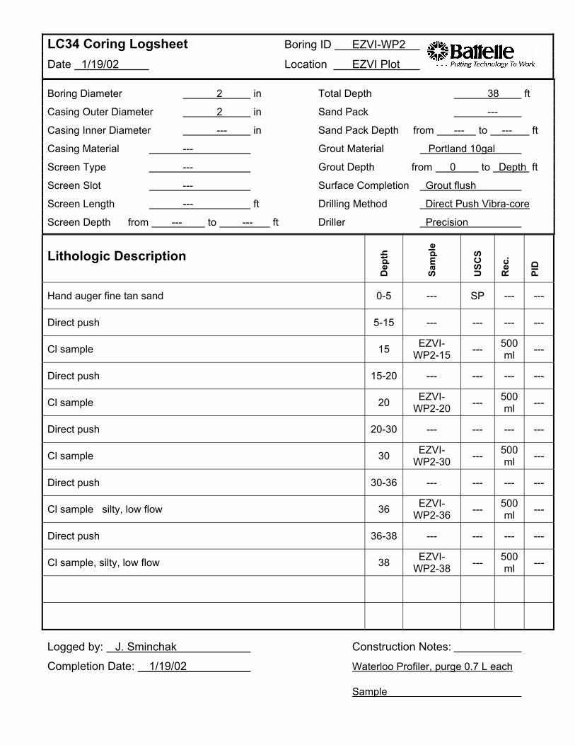
LC34 Coring Logsheet Date 1/19/02

Boring ID EZVI-WP2

Location EZVI Plot

Boring Diameter

Casing Outer Diameter

Casing Inner Diameter

Casing Material

Screen Type ---

Screen Slot ---

Screen Length

Screen Depth from

---

---

---

2

2

to

---

in

in

in

ft

---

Total Depth 38 ft

Sand Pack ---

Sand Pack Depth from to ft

Grout Material Portland 10gal

Grout Depth from 0 to Depth ft

Surface Completion Grout flush

Drilling Method Direct Push Vibra-core

ft Driller Precision

--- ---

Lithologic Description

Dep

th

Sam

ple

USC

S

Rec

.

PID

Hand auger fine tan sand 0-5 --- SP --- ---

Direct push 5-15 --- --- --- ---

Cl sample 15 EZVI­WP2-15 --- 500

ml ---

Direct push 15-20 --- --- --- ---

Cl sample 20 EZVI­WP2-20 --- 500

ml ---

Direct push 20-30 --- --- --- ---

Cl sample 30 EZVI-WP2-30 --- 500

ml ---

Direct push 30-36 --- --- --- ---

Cl sample silty, low flow 36 EZVI-WP2-36 --- 500

ml ---

Direct push 36-38 --- --- --- ---

Cl sample, silty, low flow 38 EZVI-WP2-38 --- 500

ml ---

Logged by: J. Sminchak Construction Notes:

Completion Date: 1/19/02 Waterloo Profiler, purge 0.7 L each

Sample

--- --- ---

--- --- ---

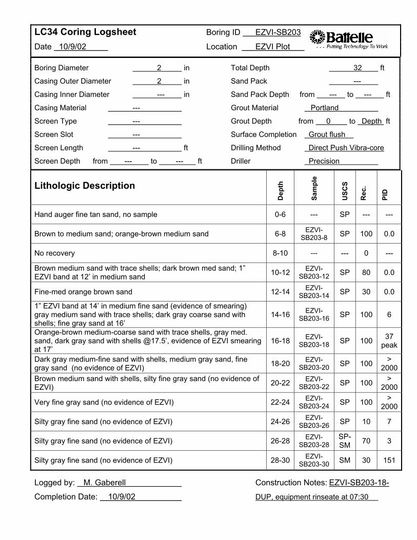
LC34 Coring Logsheet Boring ID EZVI-SB203

Date 10/9/02 Location EZVI Plot

Boring Diameter 2 in Total Depth 32 ft

Casing Outer Diameter 2 in Sand Pack ---

Casing Inner Diameter --- in Sand Pack Depth from --- to --- ft

Casing Material --- Grout Material Portland

Screen Type --- Grout Depth from 0 to Depth ft

Screen Slot --- Surface Completion Grout flush

Screen Length --- ft Drilling Method Direct Push Vibra-core

Screen Depth from --- to --- ft Driller Precision

Lithologic Description

Hand auger fine tan sand, no sample 0-6 SP

EZVI-Brown to medium sand; orange-brown medium sand 6-8 SP 100 0.0SB203-8

No recovery 8-10 0

Brown medium sand with trace shells; dark brown med sand; 1” EZVI­10-12 SP 80 0.0SB203-12 EZVI band at 12’ in medium sand D

epth

EZVI-Fine-med orange brown sand 12-14 SP 30 0.0SB203-14

1” EZVI band at 14’ in medium fine sand (evidence of smearing) EZVI-Sa

mpl

e gray medium sand with trace shells; dark gray coarse sand with 14-16 SP 100 6SB203-16 shells; fine gray sand at 16’ Orange-brown medium-coarse sand with trace shells, gray med. 37EZVI-sand, dark gray sand with shells @17.5’, evidence of EZVI smearing 16-18 SP 100SB203-18

USC

Speakat 17’

Dark gray medium-fine sand with shells, medium gray sand, fine >EZVI-R

ec.

18-20 SP 100SB203-20 gray sand (no evidence of EZVI) 2000 Brown medium sand with shells, silty fine gray sand (no evidence of >EZVI­20-22 SP 100

PID

SB203-22 EZVI) 2000 EZVI­ >Very fine gray sand (no evidence of EZVI) 22-24 SP 100SB203-24 2000 EZVI-Silty gray fine sand (no evidence of EZVI) 24-26 SP 10 7SB203-26

EZVI­ SP-Silty gray fine sand (no evidence of EZVI) 26-28 70 3SB203-28 SM EZVI-Silty gray fine sand (no evidence of EZVI) 28-30 SM 30 151SB203-30

Logged by: M. Gaberell Construction Notes: EZVI-SB203-18­

Completion Date: 10/9/02 DUP, equipment rinseate at 07:30

LC34 Coring Logsheet Date 10/9/02

Boring ID

Location

EZVI-SB203

EZVI Plot

Lithologic Description

Dep

th

Sam

ple

USC

S

Rec

.

PID

Silty gray fine sand (no evidence of EZVI) 30­32

EZVI­SB203-32 SM 80 >

2000

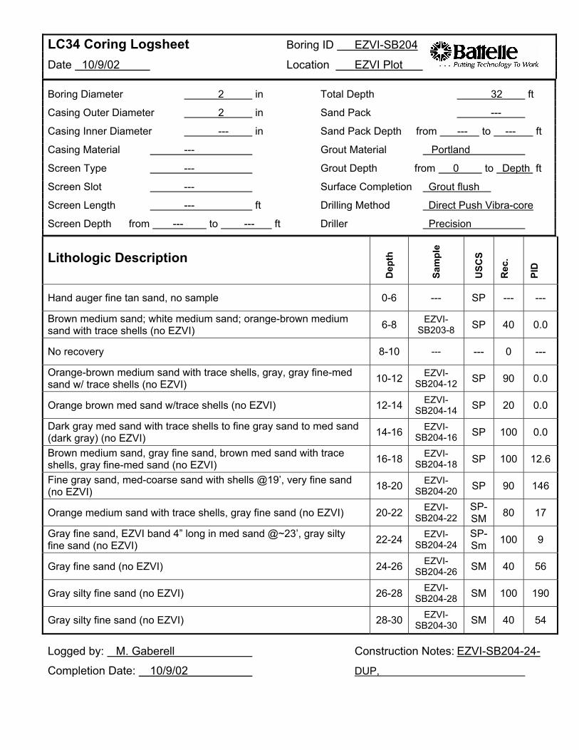
LC34 Coring Logsheet Boring ID EZVI-SB204

Date 10/9/02 Location EZVI Plot

Boring Diameter 2 in Total Depth 32 ft

Casing Outer Diameter 2 in Sand Pack ---

Casing Inner Diameter --- in Sand Pack Depth from --- to --- ft

Casing Material --- Grout Material Portland

Screen Type --- Grout Depth from 0 to Depth ft

Screen Slot --- Surface Completion Grout flush

Screen Length --- ft Drilling Method Direct Push Vibra-core

Screen Depth from --- to --- ft Driller Precision

Lithologic Description

Dep

th

Sam

ple

USC

S

Rec

.

PID

Hand auger fine tan sand, no sample 0-6 --- SP --- ---

Brown medium sand; white medium sand; orange-brown medium sand with trace shells (no EZVI) 6-8 EZVI­

SB203-8 SP 40 0.0

No recovery 8-10 --- --- 0 ---

Orange-brown medium sand with trace shells, gray, gray fine-med sand w/ trace shells (no EZVI) 10-12 EZVI­

SB204-12 SP 90 0.0

Orange brown med sand w/trace shells (no EZVI) 12-14 EZVI-SB204-14 SP 20 0.0

Dark gray med sand with trace shells to fine gray sand to med sand (dark gray) (no EZVI) 14-16 EZVI­

SB204-16 SP 100 0.0

Brown medium sand, gray fine sand, brown med sand with trace shells, gray fine-med sand (no EZVI) 16-18 EZVI­

SB204-18 SP 100 12.6

Fine gray sand, med-coarse sand with shells @19’, very fine sand (no EZVI) 18-20 EZVI­

SB204-20 SP 90 146

Orange medium sand with trace shells, gray fine sand (no EZVI) 20-22 EZVI-SB204-22

SP­SM 80 17

Gray fine sand, EZVI band 4” long in med sand @~23’, gray silty fine sand (no EZVI) 22-24 EZVI­

SB204-24 SP­Sm 100 9

Gray fine sand (no EZVI) 24-26 EZVI-SB204-26 SM 40 56

Gray silty fine sand (no EZVI) 26-28 EZVI-SB204-28 SM 100 190

Gray silty fine sand (no EZVI) 28-30 EZVI-SB204-30 SM 40 54

Logged by: M. Gaberell Construction Notes: EZVI-SB204-24­

Completion Date: 10/9/02 DUP,

LC34 Coring Logsheet Date 10/9/02

Boring ID

Location

EZVI-SB204

EZVI Plot

Lithologic Description

Dep

th

Sam

ple

USC

S

Rec

.

PID

Silty gray fine sand (no evidence of EZVI) 30­32

EZVI­SB204-32 SM 100 19

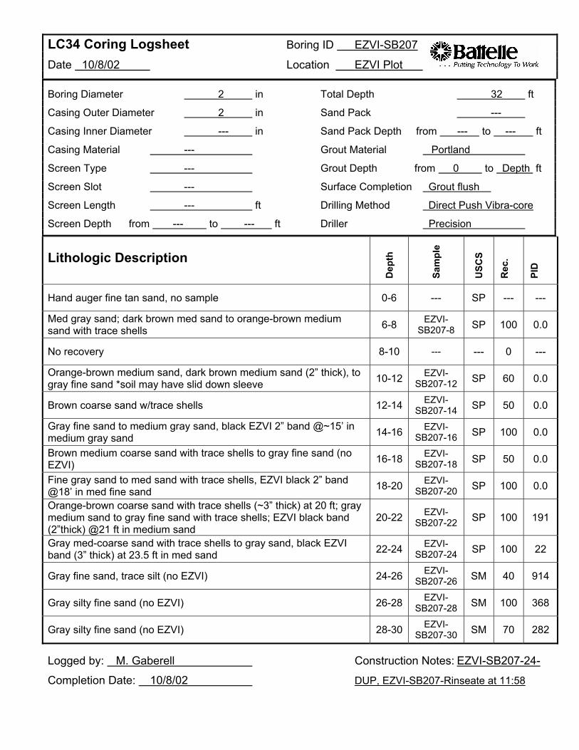
LC34 Coring Logsheet Boring ID EZVI-SB207

Date 10/8/02 Location EZVI Plot

Boring Diameter 2 in Total Depth 32 ft

Casing Outer Diameter 2 in Sand Pack ---

Casing Inner Diameter in Sand Pack Depth from to ft

Casing Material Grout Material Portland

Screen Type --- Grout Depth from 0 to Depth ft

Screen Slot --- Surface Completion Grout flush

Screen Length ft Drilling Method Direct Push Vibra-core

Screen Depth from to ft Driller Precision

--- --- ---

---

---

--- ---

Lithologic Description

Dep

th

Sam

ple

USC

S

Rec

.

PID

Hand auger fine tan sand, no sample 0-6 --- SP --- ---

Med gray sand; dark brown med sand to orange-brown medium sand with trace shells 6-8 EZVI­

SB207-8 SP 100 0.0

No recovery 8-10 --- --- 0 ---

Orange-brown medium sand, dark brown medium sand (2” thick), to gray fine sand *soil may have slid down sleeve 10-12 EZVI­

SB207-12 SP 60 0.0

Brown coarse sand w/trace shells 12-14 EZVI­SB207-14 SP 50 0.0

Gray fine sand to medium gray sand, black EZVI 2” band @~15’ in medium gray sand 14-16 EZVI­

SB207-16 SP 100 0.0

Brown medium coarse sand with trace shells to gray fine sand (no EZVI) 16-18 EZVI­

SB207-18 SP 50 0.0

Fine gray sand to med sand with trace shells, EZVI black 2” band @18’ in med fine sand 18-20 EZVI­

SB207-20 SP 100 0.0

Orange-brown coarse sand with trace shells (~3” thick) at 20 ft; gray medium sand to gray fine sand with trace shells; EZVI black band (2”thick) @21 ft in medium sand

20-22 EZVI­SB207-22 SP 100 191

Gray med-coarse sand with trace shells to gray sand, black EZVI band (3” thick) at 23.5 ft in med sand 22-24 EZVI­

SB207-24 SP 100 22

Gray fine sand, trace silt (no EZVI) 24-26 EZVI­SB207-26 SM 40 914

Gray silty fine sand (no EZVI) 26-28 EZVI­SB207-28 SM 100 368

Gray silty fine sand (no EZVI) 28-30 EZVI­SB207-30 SM 70 282

Logged by: M. Gaberell Construction Notes: EZVI-SB207-24­

Completion Date: 10/8/02 DUP, EZVI-SB207-Rinseate at 11:58

LC34 Coring Logsheet Date 10/8/02

Boring ID

Location

EZVI-SB207

EZVI Plot

Lithologic Description

Dep

th

Sam

ple

USC

S

Rec

.

PID

Silty gray fine sand (no evidence of EZVI) 30­32

EZVI­SB207-32 SM 100 49.5

--- --- ---

--- --- ---

--- --- ---

--- --- ---

--- --- ---

--- --- ---

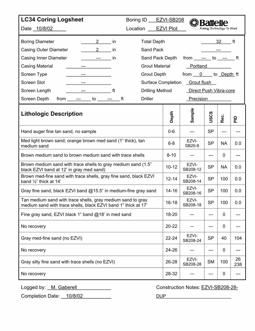
LC34 Coring Logsheet Boring ID EZVI-SB208

Date 10/8/02 Location EZVI Plot

Boring Diameter 2 in Total Depth 32 ft

Casing Outer Diameter 2 in Sand Pack ---

Casing Inner Diameter --- in Sand Pack Depth from --- to --- ft

Casing Material --- Grout Material Portland

Screen Type --- Grout Depth from 0 to Depth ft

Screen Slot --- Surface Completion Grout flush

Screen Length --- ft Drilling Method Direct Push Vibra-core

Screen Depth from --- to --- ft Driller Precision

Lithologic Description

Hand auger fine tan sand, no sample 0-6 SP

Med light brown sand; orange brown med sand (1” thick), tan EZVI­6-8 SP NA 0.0SB20-8medium sand

Brown medium sand to brown medium sand with trace shells 8-10 0

Brown medium sand with trace shells to gray medium sand (1.5” EZVI­10-12 SP NA 0.0SB208-12 black EZVI band at 12’ in gray med sand) D

epth

Brown med-fine sand with trace shells, gray fine sand, black EZVI EZVI­12-14 SP 100 0.0SB208-14

EZVI-band ½” thick at 14’

Gray fine sand, black EZVI band @15.5” in medium-fine gray sand 14-16 SP 100 0.0 Sa

mpl

e SB208-16

Tan medium sand with trace shells, gray medium sand to gray EZVI­16-18 SP 100 0.0SB208-18 medium sand with trace shells, black EZVI band 1” thick at 17’ U

SCS

Fine gray sand, EZVI black 1” band @18’ in med sand 18-20 0

Rec

. No recovery 20-22 0

EZVI­PI

D

Gray med-fine sand (no EZVI) 22-24 SP 40 104SB208-24

No recovery 24-26 0

EZVI­ 26Gray silty fine sand with trace shells (no EZVI) 26-28 SM 100SB208-28 238

No recovery 28-32 0

Logged by: M. Gaberell Construction Notes: EZVI-SB208-28­

Completion Date: 10/8/02 DUP

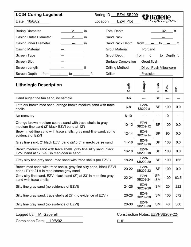
LC34 Coring Logsheet Boring ID EZVI-SB209

Date 10/8/02 Location EZVI Plot

Boring Diameter 2 in Total Depth 32 ft

Casing Outer Diameter 2 in Sand Pack ---

Casing Inner Diameter in Sand Pack Depth from to ft

Casing Material Grout Material Portland

Screen Type --- Grout Depth from 0 to Depth ft

Screen Slot --- Surface Completion Grout flush

Screen Length ft Drilling Method Direct Push Vibra-core

Screen Depth from to ft Driller Precision

--- --- ---

---

---

--- ---

Lithologic Description

Dep

th

Sam

ple

USC

S

Rec

.

PID

Hand auger fine tan sand, no sample 0-6 --- SP --- ---

Lt to drk brown med sand, orange brown medium sand with trace shells 6-8 EZVI­

SB209-8 SP 100 0.0

No recovery 8-10 --- --- 0 ---

Orange-brown medium-coarse sand with trace shells to gray medium-fine sand (2” black EZVI band at 12’) 10-12 EZVI­

SB209-12 SP 100 0.0

Brown med-fine sand with trace shells, gray med-fine sand, some evidence of EZVI 12-14 EZVI­

SB209-14 SP 90 0.0

Gray fine sand, 2” black EZVI band @15.5” in med-coarse sand 14-16 EZVI­SB209-16 SP 100 0.0

Brown medium sand with trace shells, gray fine sility sand, black EZVI band at 17.5-18’ in med-coarse sand’ 16-18 EZVI­

SB209-18 SP 100 0.0

Gray silty fine gray sand, med sand with trace shells (no EZVI) 18-20 EZVI­SB209-20 SP 100 165

Brown med sand with trace shells, gray fine silty sand, black EZVI band (1”) at 21 ft in med coarse gray sand 20-22 EZVI­

SB209-22 SP 100 0.0

Gray silty fine sand, EZVI black band (2”) at 23” in med fine gray sand with trace shells 22-24 EZVI­

SB209-24 SP­SM 100 63.5

Silty fine gray sand (no evidence of EZVI) 24-26 EZVI­SB209-26 SM 20 222

Silty fine gray sand, trace shells at 27’ (no evidence of EZVI) 26-28 EZVI­SB209-28 SM 100 572

Silty fine gray sand (no evidence of EZVI) 28-30 EZVI­SB209-30 SM 40 300

Logged by: M. Gaberell Construction Notes: EZVI-SB209-22­

Completion Date: 10/8/02 DUP

LC34 Coring Logsheet Boring ID

Date 10/8/02 Location

EZVI-SB209

EZVI Plot

Lithologic Description

Dep

th

Sam

ple

USC

S

Rec

.

PID

Silty gray fine sand, very wet at 32’ (no evidence of EZVI) 30­32 X SM 100 ---

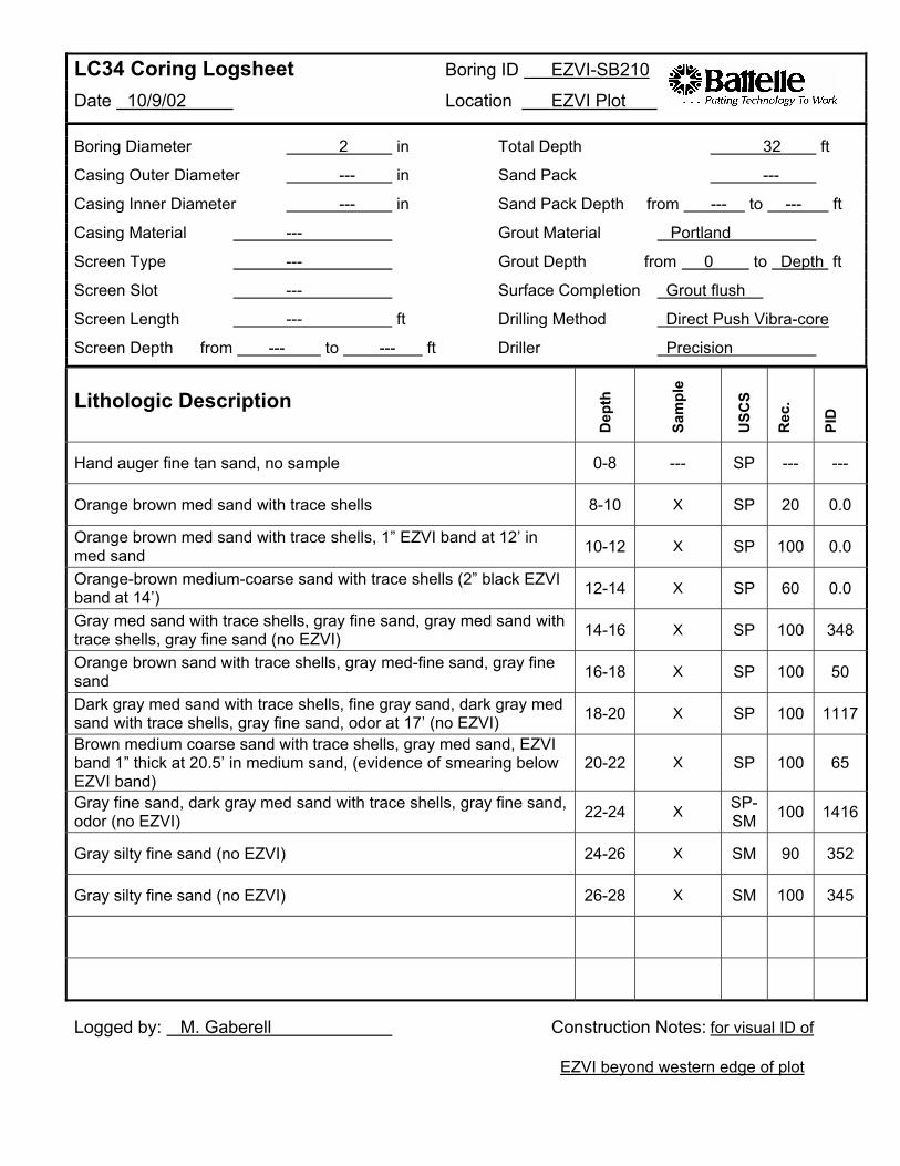
LC34 Coring Logsheet Boring ID EZVI-SB210

Date 10/9/02 Location EZVI Plot

Boring Diameter 2 in Total Depth 32 ft

Casing Outer Diameter in Sand Pack ---

Casing Inner Diameter in Sand Pack Depth from to ft

Casing Material Grout Material Portland

Screen Type --- Grout Depth from 0 to Depth ft

Screen Slot --- Surface Completion Grout flush

Screen Length ft Drilling Method Direct Push Vibra-core

Screen Depth from to ft Driller Precision

---

--- --- ---

---

---

--- ---

Lithologic Description

Dep

th

Sam

ple

USC

S

Rec

.

PID

Hand auger fine tan sand, no sample 0-8 --- SP --- ---

Orange brown med sand with trace shells 8-10 X SP 20 0.0

Orange brown med sand with trace shells, 1” EZVI band at 12’ in med sand 10-12 X SP 100 0.0

Orange-brown medium-coarse sand with trace shells (2” black EZVI band at 14’) 12-14 X SP 60 0.0

Gray med sand with trace shells, gray fine sand, gray med sand with trace shells, gray fine sand (no EZVI) 14-16 X SP 100 348

Orange brown sand with trace shells, gray med-fine sand, gray fine sand 16-18 X SP 100 50

Dark gray med sand with trace shells, fine gray sand, dark gray med sand with trace shells, gray fine sand, odor at 17’ (no EZVI) 18-20 X SP 100 1117

Brown medium coarse sand with trace shells, gray med sand, EZVI band 1” thick at 20.5’ in medium sand, (evidence of smearing below EZVI band)

20-22 X SP 100 65

Gray fine sand, dark gray med sand with trace shells, gray fine sand, odor (no EZVI) 22-24 X SP­

SM 100 1416

Gray silty fine sand (no EZVI) 24-26 X SM 90 352

Gray silty fine sand (no EZVI) 26-28 X SM 100 345

Logged by: M. Gaberell Construction Notes: for visual ID of

EZVI beyond western edge of plot

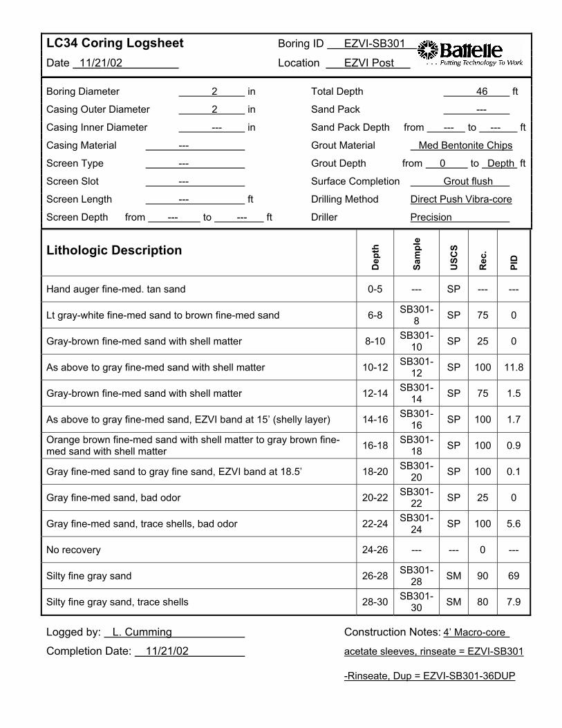
LC34 Coring Logsheet Date 11/21/02

Boring ID

Location

EZVI-SB301

EZVI Post

Boring Diameter 2 in Total Depth 46 ft

Casing Outer Diameter 2 in Sand Pack ---

Casing Inner Diameter --- in Sand Pack Depth from --- to --- ft

Casing Material --- Grout Material Med Bentonite Chips

Screen Type --- Grout Depth from 0 to Depth ft

Screen Slot --- Surface Completion Grout flush

Screen Length --- ft Drilling Method Direct Push Vibra-core

Screen Depth from --- to --- ft Driller Precision

Lithologic Description

Dep

th

Sam

ple

USC

S

Rec

.

PID

Hand auger fine-med. tan sand 0-5 --- SP --- ---

Lt gray-white fine-med sand to brown fine-med sand 6-8 SB301­8 SP 75 0

Gray-brown fine-med sand with shell matter 8-10 SB301­10 SP 25 0

As above to gray fine-med sand with shell matter 10-12 SB301­12 SP 100 11.8

Gray-brown fine-med sand with shell matter 12-14 SB301­14 SP 75 1.5

As above to gray fine-med sand, EZVI band at 15’ (shelly layer) 14-16 SB301­16 SP 100 1.7

Orange brown fine-med sand with shell matter to gray brown fine­med sand with shell matter 16-18 SB301­

18 SP 100 0.9

Gray fine-med sand to gray fine sand, EZVI band at 18.5’ 18-20 SB301­20 SP 100 0.1

Gray fine-med sand, bad odor 20-22 SB301­22 SP 25 0

Gray fine-med sand, trace shells, bad odor 22-24 SB301­24 SP 100 5.6

No recovery 24-26 --- --- 0 ---

Silty fine gray sand 26-28 SB301­28 SM 90 69

Silty fine gray sand, trace shells 28-30 SB301­30 SM 80 7.9

Logged by: L. Cumming Construction Notes: 4’ Macro-core

Completion Date: 11/21/02 acetate sleeves, rinseate = EZVI-SB301

-Rinseate, Dup = EZVI-SB301-36DUP

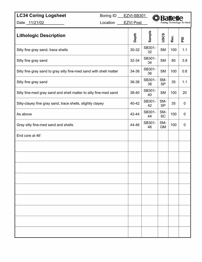
LC34 Coring Logsheet Boring ID

Date 11/21/02 Location

EZVI-SB301

EZVI Post

Lithologic Description

Dep

th

Sam

ple

USC

S

Rec

.

PID

Silty fine gray sand, trace shells 30-32 SB301­32 SM 100 1.1

Silty fine gray sand 32-34 SB301­34 SM 80 3.9

Silty fine gray sand to gray silty fine-med sand with shell matter 34-36 SB301­36 SM 100 0.8

Silty fine gray sand 36-38 SB301­38

SM­SP 35 1.1

Silty fine-med gray sand and shell matter to silty fine-med sand 38-40 SB301­40 SM 100 20

Silty-clayey fine gray sand, trace shells, slightly clayey 40-42 SB301­42

SM­SP 35 0

As above 42-44 SB301­44

SM­SC 100 0

Gray silty fine-med sand and shells 44-46 SB301­46

SM­GM 100 0

End core at 46’

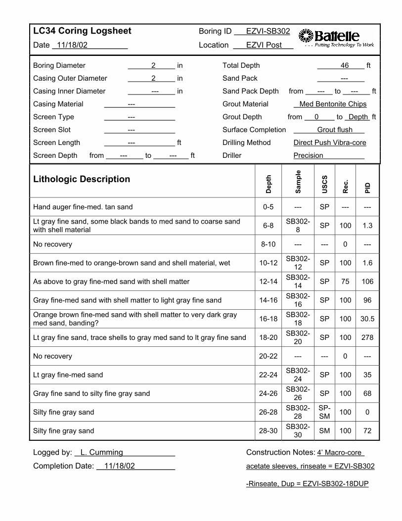
LC34 Coring Logsheet Boring ID EZVI-SB302

Date 11/18/02 Location EZVI Post

Boring Diameter 2 in Total Depth 46 ft

Casing Outer Diameter 2 in Sand Pack ---

Casing Inner Diameter --- in Sand Pack Depth from --- to --- ft

Casing Material --- Grout Material Med Bentonite Chips

Screen Type --- Grout Depth from 0 to Depth ft

Screen Slot --- Surface Completion Grout flush

Screen Length --- ft Drilling Method Direct Push Vibra-core

Screen Depth from --- to --- ft Driller Precision

Lithologic Description

Dep

th

Sam

ple

USC

S

Rec

.

PID

Hand auger fine-med. tan sand 0-5 --- SP --- ---

Lt gray fine sand, some black bands to med sand to coarse sand with shell material 6-8 SB302­

8 SP 100 1.3

No recovery 8-10 --- --- 0 ---

Brown fine-med to orange-brown sand and shell material, wet 10-12 SB302­12 SP 100 1.6

As above to gray fine-med sand with shell matter 12-14 SB302­14 SP 75 106

Gray fine-med sand with shell matter to light gray fine sand 14-16 SB302­16 SP 100 96

Orange brown fine-med sand with shell matter to very dark gray med sand, banding? 16-18 SB302­

18 SP 100 30.5

Lt gray fine sand, trace shells to gray med sand to lt gray fine sand 18-20 SB302­20 SP 100 278

No recovery 20-22 --- --- 0 ---

Lt gray fine-med sand 22-24 SB302­24 SP 100 35

Gray fine sand to silty fine gray sand 24-26 SB302­26 SP 100 68

Silty fine gray sand 26-28 SB302­28

SP-SM 100 0

Silty fine gray sand 28-30 SB302­30 SM 100 72

Logged by: L. Cumming Construction Notes: 4’ Macro-core

Completion Date: 11/18/02 acetate sleeves, rinseate = EZVI-SB302

-Rinseate, Dup = EZVI-SB302-18DUP

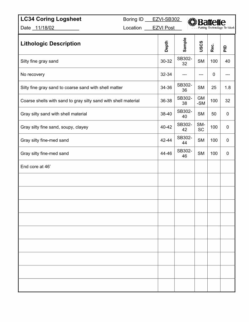
LC34 Coring Logsheet Boring ID

Date 11/18/02 Location

EZVI-SB302

EZVI Post

Lithologic Description

Dep

th

Sam

ple

USC

S

Rec

.

PID

Silty fine gray sand 30-32 SB302­32 SM 100 40

No recovery 32-34 --- --- 0 ---

Silty fine gray sand to coarse sand with shell matter 34-36 SB302­36 SM 25 1.8

Coarse shells with sand to gray silty sand with shell material 36-38 SB302­38

GM -SM 100 32

Gray silty sand with shell material 38-40 SB302­40 SM 50 0

Gray silty fine sand, soupy, clayey 40-42 SB302­42

SM­SC 100 0

Gray silty fine-med sand 42-44 SB302­44 SM 100 0

Gray silty fine-med sand 44-46 SB302­46 SM 100 0

End core at 46’

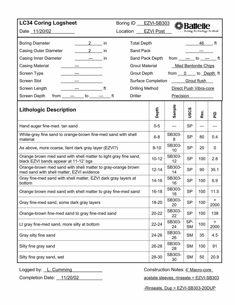
LC34 Coring Logsheet Boring ID EZVI-SB303

Date 11/20/02 Location EZVI Post

Boring Diameter 2 in Total Depth 46 ft

Casing Outer Diameter 2 in Sand Pack ---

Casing Inner Diameter --- in Sand Pack Depth from --- to --- ft

Casing Material --- Grout Material Med Bentonite Chips

Screen Type --- Grout Depth from 0 to Depth ft

Screen Slot --- Surface Completion Grout flush

Screen Length --- ft Drilling Method Direct Push Vibra-core

Screen Depth from --- to --- ft Driller Precision

Lithologic Description

Dep

th

Sam

ple

USC

S

Rec

.

PID

Hand auger fine-med. tan sand 0-5 --- SP --- ---

White-gray fine sand to orange-brown fine-med sand with shell material 6-8 SB303­

8 SP 80 0.4

As above, more coarse, faint dark gray layer (EZVI?) 8-10 SB303­10 SP 20 0

Orange brown med sand with shell matter to light gray fine sand, black EZVI bands appear at 11-12’ bgs 10-12 SB303­

12 SP 100 2.8

Orange-brown med sand with shell matter to gray-orange brown med sand with shell matter, EZVI evidence 12-14 SB303­

14 SP 90 35.1

Gray fine-med sand with shell matter, EZVI dark gray layers at bottom 14-16 SB303­

16 SP 100 6.9

Orange brown med sand with shell matter to gray fine-med sand 16-18 SB303­18 SP 100 11.5

Gray fine-med sand, some dark gray layers 18-20 SB303­20 SP 100 >

2000

Orange-brown fine-med sand to gray fine-med sand 20-22 SB303­22 SP 100 138

Lt gray fine-med sand, more silty at bottom 22-24 SB303­24

SP­SM 100 >

2000

Gray silty fine sand 24-26 SB303­26 SM 35 4.5

Silty fine gray sand 26-28 SB303­28 SM 100 91

Silty fine gray sand, wet 28-30 SB303­30 SM 50 20.9

Logged by: L. Cumming Construction Notes: 4’ Macro-core

Completion Date: 11/20/02 acetate sleeves, rinseate = EZVI-SB303

-Rinseate, Dup = EZVI-SB303-20DUP

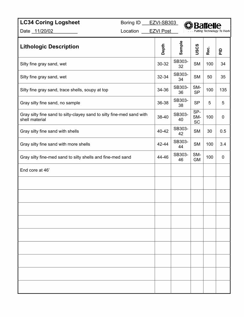
LC34 Coring Logsheet Boring ID

Date 11/20/02 Location

EZVI-SB303

EZVI Post

Lithologic Description

Dep

th

Sam

ple

USC

S

Rec

.

PID

Silty fine gray sand, wet 30-32 SB303­32 SM 100 34

Silty fine gray sand, wet 32-34 SB303­34 SM 50 35

Silty fine gray sand, trace shells, soupy at top 34-36 SB303­36

SM­SP 100 135

Gray silty fine sand, no sample 36-38 SB303­38 SP 5 5

Gray silty fine sand to silty-clayey sand to silty fine-med sand with shell material 38-40 SB303­

40

SP­SM­SC

100 0

Gray silty fine sand with shells 40-42 SB303­42 SM 30 0.5

Gray silty fine sand with more shells 42-44 SB303­44 SM 100 3.4

Gray silty fine-med sand to silty shells and fine-med sand 44-46 SB303­46

SM­GM 100 0

End core at 46’

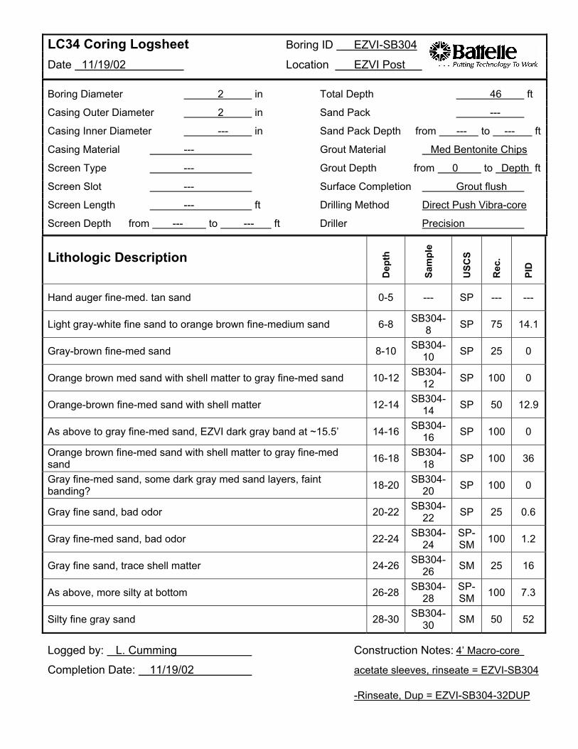
LC34 Coring Logsheet Boring ID EZVI-SB304

Date 11/19/02 Location EZVI Post

Boring Diameter 2 in Total Depth 46 ft

Casing Outer Diameter 2 in Sand Pack ---

Casing Inner Diameter --- in Sand Pack Depth from --- to --- ft

Casing Material --- Grout Material Med Bentonite Chips

Screen Type --- Grout Depth from 0 to Depth ft

Screen Slot --- Surface Completion Grout flush

Screen Length --- ft Drilling Method Direct Push Vibra-core

Screen Depth from --- to --- ft Driller Precision

Lithologic Description

Dep

th

Sam

ple

USC

S

Rec

.

PID

Hand auger fine-med. tan sand 0-5 --- SP --- ---

Light gray-white fine sand to orange brown fine-medium sand 6-8 SB304­8 SP 75 14.1

Gray-brown fine-med sand 8-10 SB304­10 SP 25 0

Orange brown med sand with shell matter to gray fine-med sand 10-12 SB304­12 SP 100 0

Orange-brown fine-med sand with shell matter 12-14 SB304­14 SP 50 12.9

As above to gray fine-med sand, EZVI dark gray band at ~15.5’ 14-16 SB304­16 SP 100 0

Orange brown fine-med sand with shell matter to gray fine-med sand 16-18 SB304­

18 SP 100 36

Gray fine-med sand, some dark gray med sand layers, faint banding? 18-20 SB304­

20 SP 100 0

Gray fine sand, bad odor 20-22 SB304­22 SP 25 0.6

Gray fine-med sand, bad odor 22-24 SB304­24

SP-SM 100 1.2

Gray fine sand, trace shell matter 24-26 SB304­26 SM 25 16

As above, more silty at bottom 26-28 SB304­28

SP-SM 100 7.3

Silty fine gray sand 28-30 SB304­30 SM 50 52

Logged by: L. Cumming Construction Notes: 4’ Macro-core

Completion Date: 11/19/02 acetate sleeves, rinseate = EZVI-SB304

-Rinseate, Dup = EZVI-SB304-32DUP

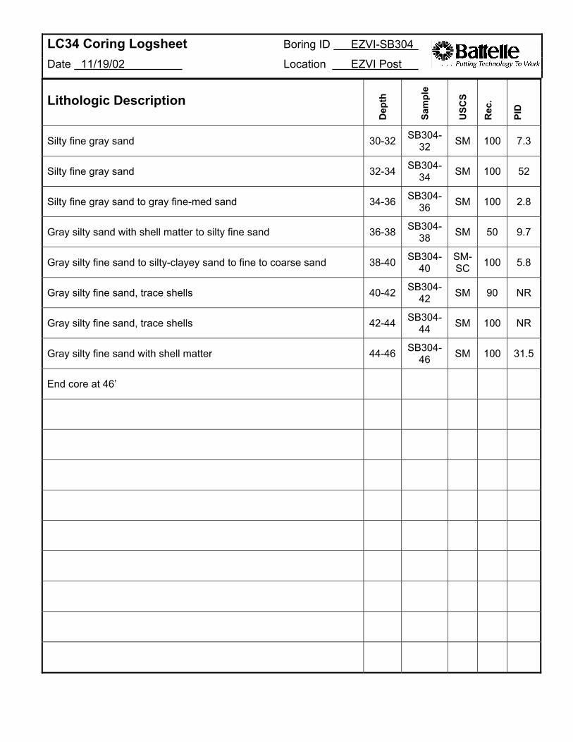
LC34 Coring Logsheet Boring ID

Date 11/19/02 Location

EZVI-SB304

EZVI Post

Lithologic Description

Dep

th

Sam

ple

USC

S

Rec

.

PID

Silty fine gray sand 30-32 SB304­32 SM 100 7.3

Silty fine gray sand 32-34 SB304­34 SM 100 52

Silty fine gray sand to gray fine-med sand 34-36 SB304­36 SM 100 2.8

Gray silty sand with shell matter to silty fine sand 36-38 SB304­38 SM 50 9.7

Gray silty fine sand to silty-clayey sand to fine to coarse sand 38-40 SB304­40

SM­SC 100 5.8

Gray silty fine sand, trace shells 40-42 SB304­42 SM 90 NR

Gray silty fine sand, trace shells 42-44 SB304­44 SM 100 NR

Gray silty fine sand with shell matter 44-46 SB304­46 SM 100 31.5

End core at 46’

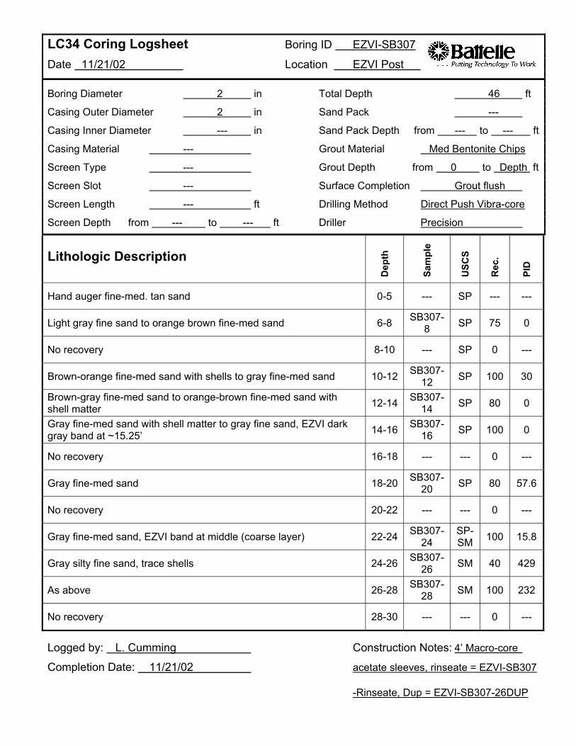
LC34 Coring Logsheet Date 11/21/02

Boring ID

Location

EZVI-SB307

EZVI Post

Boring Diameter 2 in Total Depth 46 ft

Casing Outer Diameter 2 in Sand Pack ---

Casing Inner Diameter --- in Sand Pack Depth from --- to --- ft

Casing Material --- Grout Material Med Bentonite Chips

Screen Type --- Grout Depth from 0 to Depth ft

Screen Slot --- Surface Completion Grout flush

Screen Length --- ft Drilling Method Direct Push Vibra-core

Screen Depth from --- to --- ft Driller Precision

Lithologic Description

Dep

th

Sam

ple

USC

S

Rec

.

PID

Hand auger fine-med. tan sand 0-5 --- SP --- ---

Light gray fine sand to orange brown fine-med sand 6-8 SB307­8 SP 75 0

No recovery 8-10 --- SP 0 ---

Brown-orange fine-med sand with shells to gray fine-med sand 10-12 SB307­12 SP 100 30

Brown-gray fine-med sand to orange-brown fine-med sand with shell matter 12-14 SB307­

14 SP 80 0

Gray fine-med sand with shell matter to gray fine sand, EZVI dark gray band at ~15.25’ 14-16 SB307­

16 SP 100 0

No recovery 16-18 --- --- 0 ---

Gray fine-med sand 18-20 SB307­20 SP 80 57.6

No recovery 20-22 --- --- 0 ---

Gray fine-med sand, EZVI band at middle (coarse layer) 22-24 SB307­24

SP-SM 100 15.8

Gray silty fine sand, trace shells 24-26 SB307­26 SM 40 429

As above 26-28 SB307­28 SM 100 232

No recovery 28-30 --- --- 0 ---

Logged by: L. Cumming Construction Notes: 4’ Macro-core

Completion Date: 11/21/02 acetate sleeves, rinseate = EZVI-SB307

-Rinseate, Dup = EZVI-SB307-26DUP

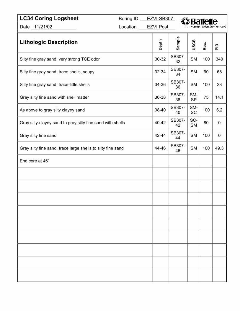
LC34 Coring Logsheet Boring ID

Date 11/21/02 Location

EZVI-SB307

EZVI Post

Lithologic Description

Dep

th

Sam

ple

USC

S

Rec

.

PID

Silty fine gray sand, very strong TCE odor 30-32 SB307­32 SM 100 340

Silty fine gray sand, trace shells, soupy 32-34 SB307­34 SM 90 68

Silty fine gray sand, trace-little shells 34-36 SB307­36 SM 100 28

Gray silty fine sand with shell matter 36-38 SB307­38

SM­SP 75 14.1

As above to gray silty clayey sand 38-40 SB307­40

SM­SC 100 6.2

Gray silty-clayey sand to gray silty fine sand with shells 40-42 SB307­42

SC­SM 80 0

Gray silty fine sand 42-44 SB307­44 SM 100 0

Gray silty fine sand, trace large shells to silty fine sand 44-46 SB307­46 SM 100 49.3

End core at 46’

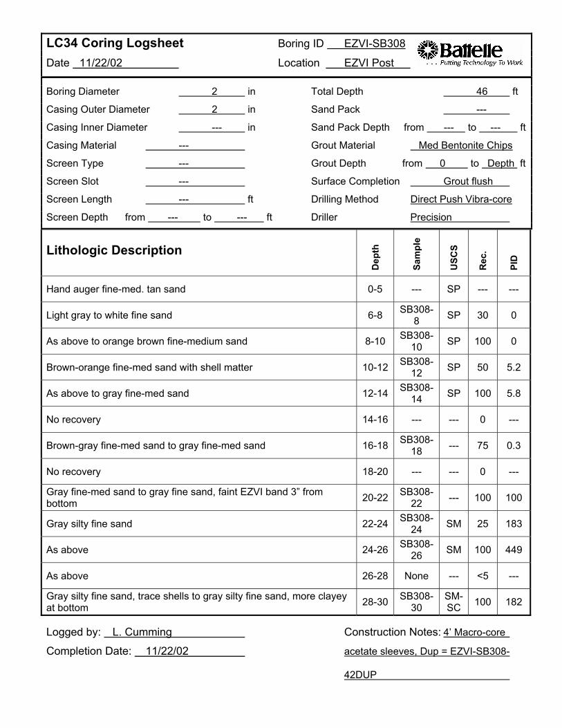
LC34 Coring Logsheet Date 11/22/02

Boring ID

Location

EZVI-SB308

EZVI Post

Boring Diameter 2 in Total Depth 46 ft

Casing Outer Diameter 2 in Sand Pack ---

Casing Inner Diameter --- in Sand Pack Depth from --- to --- ft

Casing Material --- Grout Material Med Bentonite Chips

Screen Type --- Grout Depth from 0 to Depth ft

Screen Slot --- Surface Completion Grout flush

Screen Length --- ft Drilling Method Direct Push Vibra-core

Screen Depth from --- to --- ft Driller Precision

Lithologic Description

Dep

th

Sam

ple

USC

S

Rec

.

PID

Hand auger fine-med. tan sand 0-5 --- SP --- ---

Light gray to white fine sand 6-8 SB308­8 SP 30 0

As above to orange brown fine-medium sand 8-10 SB308­10 SP 100 0

Brown-orange fine-med sand with shell matter 10-12 SB308­12 SP 50 5.2

As above to gray fine-med sand 12-14 SB308­14 SP 100 5.8

No recovery 14-16 --- --- 0 ---

Brown-gray fine-med sand to gray fine-med sand 16-18 SB308­18 --- 75 0.3

No recovery 18-20 --- --- 0 ---

Gray fine-med sand to gray fine sand, faint EZVI band 3” from bottom 20-22 SB308­

22 --- 100 100

Gray silty fine sand 22-24 SB308­24 SM 25 183

As above 24-26 SB308­26 SM 100 449

As above 26-28 None --- <5 ---

Gray silty fine sand, trace shells to gray silty fine sand, more clayey at bottom 28-30 SB308­

30 SM­SC 100 182

Logged by: L. Cumming Construction Notes: 4’ Macro-core

Completion Date: 11/22/02 acetate sleeves, Dup = EZVI-SB308­

42DUP

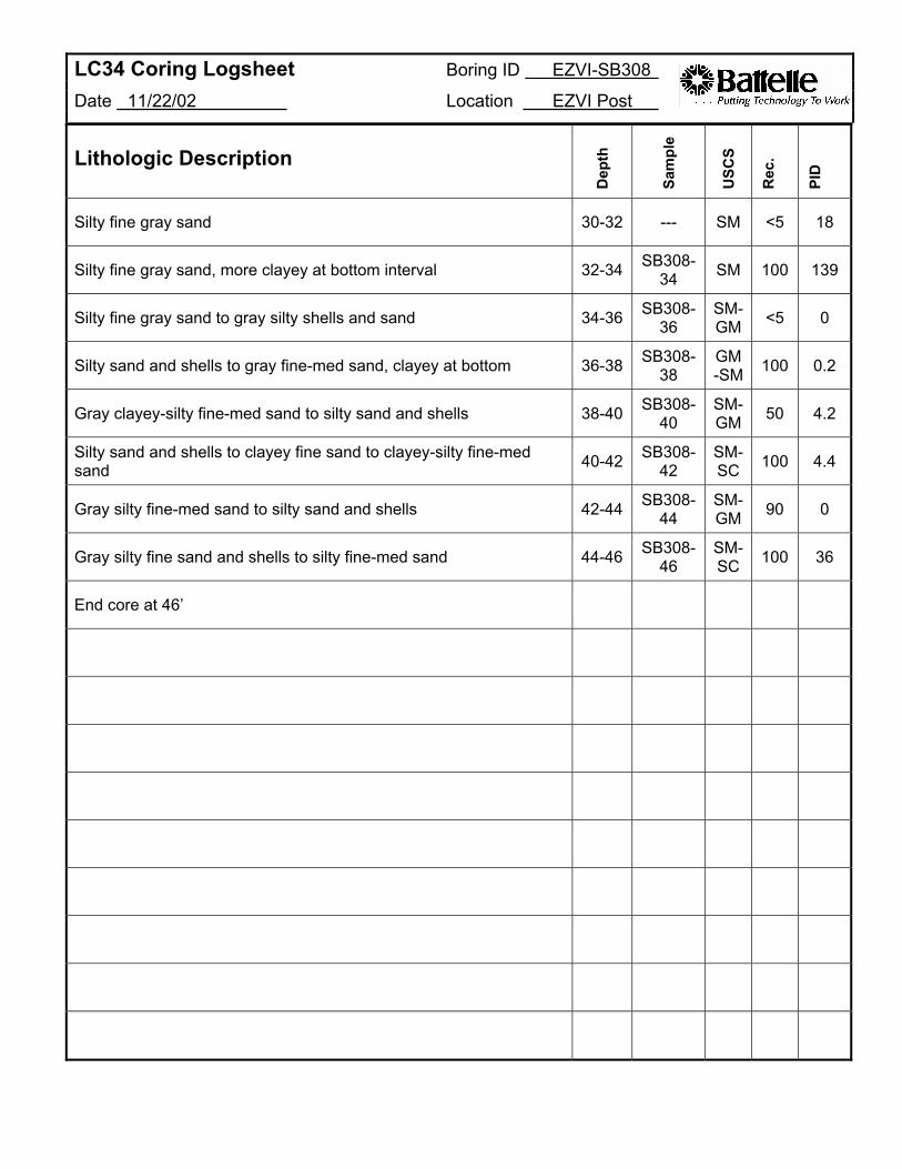
LC34 Coring Logsheet Boring ID

Date 11/22/02 Location

EZVI-SB308

EZVI Post

Lithologic Description

Dep

th

Sam

ple

USC

S

Rec

.

PID

Silty fine gray sand 30-32 --- SM <5 18

Silty fine gray sand, more clayey at bottom interval 32-34 SB308­34 SM 100 139

Silty fine gray sand to gray silty shells and sand 34-36 SB308­36

SM­GM <5 0

Silty sand and shells to gray fine-med sand, clayey at bottom 36-38 SB308­38

GM -SM 100 0.2

Gray clayey-silty fine-med sand to silty sand and shells 38-40 SB308­40

SM­GM 50 4.2

Silty sand and shells to clayey fine sand to clayey-silty fine-med sand 40-42 SB308­

42 SM­SC 100 4.4

Gray silty fine-med sand to silty sand and shells 42-44 SB308­44

SM­GM 90 0

Gray silty fine sand and shells to silty fine-med sand 44-46 SB308­46

SM­SC 100 36

End core at 46’

Appendix C CVOC Measurements

Table C-1. CVOC Results of Groundwater Samples Table C-2. Summary of CVOC Results in Soil from EZVI Pre-

Demonstration Monitoring Table C-3. Summary of CVOC Results in Soil from EZVI Intermediate

Monitoring Table C-4. Summary of CVOC Results in Soil from EZVI Post-

Demonstration Monitoring Table C-5. Long-Term Groundwater Sampling

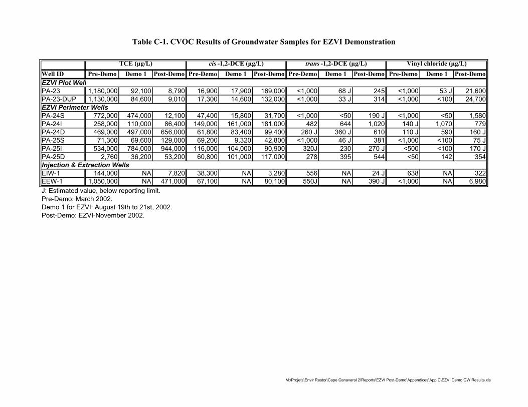
Table C-1. CVOC Results of Groundwater Samples for EZVI Demonstration

TCE (µg/L) cis -1,2-DCE (µg/L) trans -1,2-DCE (µg/L) Vinyl chloride (µg/L) Well ID Pre-Demo Demo 1 Post-Demo Pre-Demo Demo 1 Post-Demo Pre-Demo Demo 1 Post-Demo Pre-Demo Demo 1 Post-Demo EZVI Plot Well PA-23 1,180,000 92,100 8,790 16,900 17,900 169,000 <1,000 68 J 245 <1,000 53 J 21,600 PA-23-DUP 1,130,000 84,600 9,010 17,300 14,600 132,000 <1,000 33 J 314 <1,000 <100 24,700 EZVI Perimeter Wells PA-24S 772,000 474,000 12,100 47,400 15,800 31,700 <1,000 <50 190 J <1,000 <50 1,580 PA-24I 258,000 110,000 86,400 149,000 161,000 181,000 482 644 1,020 140 J 1,070 779 PA-24D 469,000 497,000 656,000 61,800 83,400 99,400 260 J 360 J 610 110 J 590 160 J PA-25S 71,300 69,600 129,000 69,200 9,320 42,800 <1,000 46 J 381 <1,000 <100 75 J PA-25I 534,000 784,000 944,000 116,000 104,000 90,900 320J 230 270 J <500 <100 170 J PA-25D 2,760 36,200 53,200 60,800 101,000 117,000 278 395 544 <50 142 354 Injection & Extraction Wells EIW-1 144,000 NA 7,820 38,300 NA 3,280 556 NA 24 J 638 NA 322 EEW-1 1,050,000 NA 471,000 67,100 NA 80,100 550J NA 390 J <1,000 NA 6,980 J: Estimated value, below reporting limit.Pre-Demo: March 2002.Demo 1 for EZVI: August 19th to 21st, 2002.Post-Demo: EZVI-November 2002.

M:\Projets\Envir Restor\Cape Canaveral 2\Reports\EZVI Post-Demo\Appendices\App C\EZVI Demo GW Results.xls

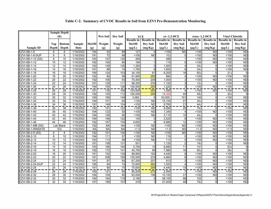
Sample Depth (ft) Wet Soil Dry Soil TCE cis -1,2-DCE trans -1,2-DCE Vinyl Chloride

Results in Results in Results in Results in Results in Results in Results in Results in Top Bottom Sample MeOH Weight Weight MeOH Dry Soil MeOH Dry Soil MeOH Dry Soil MeOH Dry Soil

Sample ID Depth Depth Date (g) (g) (g) (µg/L) (mg/Kg) (µg/L) (mg/Kg) (µg/L) (mg/Kg) (µg/L) (mg/Kg) EZVI-SB-1-8 6 8 1/16/2002 194 93 89 121 0 <100 ND <100 ND <100 ND EZVI-SB-1-8-DUP 6 8 1/16/2002 191 72 68 <100 ND 10J 0 <100 ND <100 ND EZVI-SB-1-10 (SS) 8 10 1/16/2002 193 147 125 459 1 488 1 <100 ND <100 ND EZVI-SB-1-12 10 12 1/16/2002 192 100 80 184 1 119 0 <100 ND <100 ND EZVI-SB-1-14 12 14 1/16/2002 192 149 126 1,300 3 1,920 4 34J 0 <100 ND EZVI-SB-1-16 14 16 1/16/2002 191 88 74 1,760 6 1,600 6 34J 0 <100 ND EZVI-SB-1-18 16 18 1/16/2002 190 124 103 34,100 87 6,200 16 60J 0 21J 0 EZVI-SB-1-20 18 20 1/16/2002 192 80 58 61,800 282 884 4 <100 ND <100 ND EZVI-SB-1-22 20 22 1/16/2002 192 106 93 75,400 208 1,000 3 <100 ND <100 ND EZVI-SB-1-24 22 24 1/16/2002 191 129 111 98,200 230 1,100 3 12J 0 <100 ND EZVI-SB-1-26 24 26 1/16/2002 194 155 126 130,000 283 1,220 3 <100 ND <100 ND EZVI-SB-1-28 26 28 1/16/2002 191 135 106 103,000 263 1,590 4 <100 ND <100 ND EZVI-SB-1-30 28 30 1/16/2002 192 145 112 104,000 256 18,300 45 49J 0 20J 0 EZVI-SB-1-32 30 32 1/16/2002 190 190 148 3,060 6 53,000 101 140 0 <100 ND EZVI-SB-1-34 32 34 1/16/2002 194 101 84 <100 ND 15,100 47 35J 0 <100 ND EZVI-SB-1-36 34 36 1/16/2002 191 149 124 <100 ND 9,760 21 44J 0 <100 ND EZVI-SB-1-38 36 38 1/16/2002 192 151 122 <100 ND 9,090 20 74J 0 <100 ND EZVI-SB-1-40 38 40 1/16/2002 194 123 93 <100 ND 1,340 4 <100 ND <100 ND EZVI-SB-1-42 40 42 1/16/2002 194 126 90 <100 ND 3,110 10 44J 0 <100 ND EZVI-SB-1-44 42 44 1/16/2002 194 146 122 140 0 3,520 8 <100 ND <100 ND EZVI-SB-1-46 44 46 1/16/2002 192 187 155 4,650 8 6,980 12 <100 ND <100 ND EZVI-SB-1-MB (SS) Lab Blank 1/16/2002 192 NA NA <100 ND <100 ND <100 ND <100 ND EZVI-SB-1-RINSATE EQ 1/16/2002 NA NA NA <1.0 ND <1.0 ND <1.0 ND <1.0 ND EZVI-SB-2-8 (SS) 6 8 1/16/2002 192 101 100 <100 ND <100 ND <100 ND <100 ND EZVI-SB-2-10 8 10 1/16/2002 194 111 97 <100 ND 118 0 <100 ND <100 ND EZVI-SB-2-12 10 12 1/16/2002 193 113 99 <100 ND 113 0 <100 ND <100 ND EZVI-SB-2-14 12 14 1/16/2002 191 158 131 501 1 1,120 2 19J 0 <100 ND EZVI-SB-2-16 14 16 1/16/2002 193 196 164 5,700 10 6,680 11 141 0 63J 0 EZVI-SB-2-18 16 18 1/16/2002 192 172 141 45,700 89 7,980 16 85J 0 38J 0 EZVI-SB-2-20 18 20 1/16/2002 191 152 130 89,800 182 4,440 9 <100 ND <100 ND EZVI-SB-2-22 20 22 1/16/2002 191 208 165 135,000 233 4,860 8 <100 ND <100 ND EZVI-SB-2-24 22 24 1/16/2002 191 97 83 67,200 207 913 3 <100 ND <100 ND EZVI-SB-2-24-DUP 22 24 1/16/2002 195 94 74 72,600 262 1,020 4 <100 ND <100 ND EZVI-SB-2-26 24 26 1/16/2002 191 90 75 75,600 259 4,440 15 <100 ND <100 ND EZVI-SB-2-28 26 28 1/16/2002 192 121 95 95,200 270 2,550 7 <100 ND <100 ND EZVI-SB-2-30 28 30 1/16/2002 194 104 85 63,000 196 10,100 31 <100 ND <100 ND EZVI-SB-2-32 30 32 1/16/2002 192 164 116 2,180 5 38,100 96 102 0 <100 ND EZVI-SB-2-34 32 34 1/16/2002 191 189 157 376 1 27,500 48 79J 0 <100 ND

M:\Projects\Envir Restor\Cape Canaveral 2\Reports\EZVI Post-Demo\Appendices\Appendix C

Table C-2. Summary of CVOC Results in Soil from EZVI Pre-Demonstration Monitoring

Table C-2. Summary of CVOC Results in Soil from EZVI Pre-Demonstration Monitoring (Continued)

Sample Depth (ft) Wet Soil Dry Soil TCE cis -1,2-DCE trans -1,2-DCE Vinyl Chloride

Sample ID Top

Depth Bottom Depth

Sample Date

MeOH (g)

Weight (g)

Weight (g)

Results in MeOH (µg/L)

Results in Dry Soil (mg/Kg)

Results in MeOH (µg/L)

Results in Dry Soil (mg/Kg)

Results in MeOH (µg/L)

Results in Dry Soil (mg/Kg)

Results in MeOH (µg/L)

Results in Dry Soil (mg/Kg)

EZVI-SB-2-36 34 36 1/16/2002 192 256 211 209 0 16,000 22 69J 0 <100 ND EZVI-SB-2-38 36 38 1/16/2002 192 193 162 110 0 8,600 15 44J 0 <100 ND EZVI-SB-2-40 38 40 1/16/2002 192 130 90 <100 ND 1,890 6 <100 ND <100 ND EZVI-SB-2-42 40 42 1/16/2002 194 192 150 <100 ND 668 1 <100 ND <100 ND EZVI-SB-2-44 42 44 1/16/2002 192 85 50 <100 ND 3,760 21 <100 ND <100 ND EZVI-SB-2-46 44 46 1/16/2002 192 211 178 <100 ND 3,180 5 <100 ND <100 ND EZVI-SB-2-MB (SS) Lab Blank 1/16/2002 191 NA NA <100 ND <100 ND <100 ND <100 ND EZVI-SB-2-RINSATE EQ 1/16/2002 NA NA NA <1.0 ND <1.0 ND <1.0 ND <1.0 ND EZVI-SB-3-8 (SS) 6 8 1/17/2002 194 134 132 <100 ND <100 ND <100 ND <100 ND EZVI-SB-3-10 8 10 1/17/2002 191 157 140 120 0 156 0 <100 ND <100 ND EZVI-SB-3-12 10 12 1/17/2002 191 134 111 107 0 124 0 <100 ND <100 ND EZVI-SB-3-14 12 14 1/17/2002 191 171 146 544 1 1,320 2 24J 0 27J 0 EZVI-SB-3-16 14 16 1/17/2002 190 167 146 3,830 7 2,920 5 60J 0 <100 ND EZVI-SB-3-18 16 18 1/17/2002 191 101 90 2,160,000 6,067 10,200 29 134 0 29J 0 EZVI-SB-3-20 18 20 1/17/2002 191 102 88 72,000 209 1,430 4 <100 ND <100 ND EZVI-SB-3-22 20 22 1/17/2002 191 109 95 72,500 195 906 2 <100 ND <100 ND EZVI-SB-3-24 22 24 1/17/2002 192 171 137 125,000 253 1,570 3 <100 ND <100 ND EZVI-SB-3-26 24 26 1/17/2002 191 144 114 114,000 272 1,180 3 <100 ND <100 ND EZVI-SB-3-28 26 28 1/17/2002 190 115 94 90,700 252 798 2 <100 ND <100 ND EZVI-SB-3-30 28 30 1/17/2002 192 114 92 118,000 340 6,040 17 12J 0 <100 ND EZVI-SB-3-32 30 32 1/17/2002 190 127 94 72,400 211 26,400 77 62J 0 19J 0 EZVI-SB-3-34 32 34 1/17/2002 194 157 125 859 2 40,400 90 83J 0 <100 ND EZVI-SB-3-36 34 36 1/17/2002 192 132 112 <100 ND 4,180 10 <100 ND <100 ND EZVI-SB-3-38 36 38 1/17/2002 192 139 118 212 0 7,220 16 17J 0 <100 ND EZVI-SB-3-40 38 40 1/17/2002 193 142 111 241 1 347 1 <100 ND <100 ND EZVI-SB-3-40-DUP 38 40 1/17/2002 191 95 44 158 1 249 2 <100 ND <100 ND EZVI-SB-3-42 40 42 1/17/2002 192 145 116 192 0 371 1 <100 ND <100 ND EZVI-SB-3-44 42 44 1/17/2002 191 118 97 <100 ND 1,540 4 <100 ND <100 ND EZVI-SB-3-46 44 46 1/17/2002 190 152 127 15,700 33 5,150 11 <100 ND <100 ND EZVI-SB-3-MB (SS) Lab Blank 1/17/2002 195 NA NA <100 ND <100 ND <100 ND <100 ND EZVI-SB-3-RINSATE EQ 1/16/2002 NA NA NA <1.0 ND <1.0 ND <1.0 ND <1.0 ND EZVI-SB-4-8 (SS) 6 8 1/17/2002 191 153 149 <100 ND <100 ND <100 ND <100 ND EZVI-SB-4-10 8 10 1/17/2002 193 215 188 139 0 154 0 <100 ND <100 ND EZVI-SB-4-12 10 12 1/17/2002 191 171 142 158 0 159 0 <100 ND <100 ND EZVI-SB-4-14 12 14 1/17/2002 190 148 130 2,770 6 1,890 4 39J 0 <100 ND EZVI-SB-4-16 14 16 1/17/2002 190 129 110 2,520 6 2,840 7 52J 0 <100 ND EZVI-SB-4-18 16 18 1/17/2002 190 119 102 17,700 45 4,570 12 67J 0 25J 0 EZVI-SB-4-20 18 20 1/17/2002 190 102 85 53,300 161 2,480 8 <100 ND <100 ND

M:\Projects\Envir Restor\Cape Canaveral 2\Reports\EZVI Post-Demo\Appendices\Appendix C

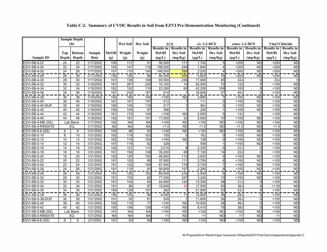
Table C-2. Summary of CVOC Results in Soil from EZVI Pre-Demonstration Monitoring (Continued)

Sample Depth (ft) Wet Soil Dry Soil TCE cis -1,2-DCE trans -1,2-DCE Vinyl Chloride

Sample ID Top

Depth Bottom Depth

Sample Date

MeOH (g)

Weight (g)

Weight (g)

Results in MeOH (µg/L)

Results in Dry Soil (mg/Kg)

Results in MeOH (µg/L)

Results in Dry Soil (mg/Kg)

Results in MeOH (µg/L)

Results in Dry Soil (mg/Kg)

Results in MeOH (µg/L)

Results in Dry Soil (mg/Kg)

EZVI-SB-4-22 20 22 1/17/2002 190 117 91 58,500 171 1,740 5 <200 ND <200 ND EZVI-SB-4-24 22 24 1/17/2002 192 147 118 108,000 249 1,840 4 <200 ND <200 ND EZVI-SB-4-26 24 26 1/17/2002 191 175 140 146,000 289 2,020 4 <200 ND <200 ND EZVI-SB-4-28 26 28 1/17/2002 192 120 98 94,300 255 5,620 15 <200 ND <200 ND EZVI-SB-4-30 28 30 1/17/2002 191 139 108 93,500 236 17,900 45 43J 0 23J 0 EZVI-SB-4-32 30 32 1/18/2002 191 281 220 10,100 14 52,500 72 122 0 <100 ND EZVI-SB-4-34 32 34 1/18/2002 192 152 110 23,300 60 42,200 109 100 0 <100 ND EZVI-SB-4-36 34 36 1/18/2002 191 230 181 514 1 16,600 27 45J 0 <100 ND EZVI-SB-4-38 36 38 1/18/2002 192 165 140 <100 ND 3,680 7 <100 ND <100 ND EZVI-SB-4-40 38 40 1/18/2002 191 167 107 512 1 111 0 <100 ND <100 ND EZVI-SB-4-40-DUP 38 40 1/18/2002 190 145 116 217 1 88J 0 <100 ND <100 ND EZVI-SB-4-42 40 42 1/18/2002 192 104 87 366 1 226 1 <100 ND <100 ND EZVI-SB-4-44 42 44 1/18/2002 191 174 144 <100 ND 2,600 5 13J 0 <100 ND EZVI-SB-4-46 44 46 1/18/2002 192 181 151 17,500 32 5,650 10 <100 ND <100 ND EZVI-SB-4-MB (SS) Lab Blank 1/17/2002 192 NA NA <100 ND <100 ND <100 ND <100 ND EZVI-SB-4-RINSATE EQ 1/17/2002 NA NA NA <1.0 ND <1.0 ND <1.0 ND <1.0 ND EZVI-SB-5-8 (SS) 6 8 1/31/2002 193 96 93 <100 ND <100 ND <100 ND <100 ND EZVI-SB-5-10 8 10 1/31/2002 192 119 103 105 0 78J 0 <100 ND <100 ND EZVI-SB-5-12 10 12 1/31/2002 192 119 104 <100 ND 128 0 <100 ND <100 ND EZVI-SB-5-14 12 14 1/31/2002 191 116 92 329 1 509 1 <100 ND <100 ND EZVI-SB-5-16 14 16 1/31/2002 192 121 114 3,510 8 2,320 5 27J 0 <100 ND EZVI-SB-5-18 16 18 1/31/2002 191 156 136 35,200 68 7,120 14 23J 0 <100 ND EZVI-SB-5-20 18 20 1/31/2002 192 120 105 46,800 115 3,630 9 <100 ND <100 ND EZVI-SB-5-22 20 22 1/31/2002 191 103 88 37,900 111 2,700 8 <100 ND <100 ND EZVI-SB-5-24 22 24 1/31/2002 191 122 100 67,400 178 2,700 7 <100 ND <100 ND EZVI-SB-5-26 24 26 1/31/2002 191 110 93 56,600 157 2,290 6 <100 ND <100 ND EZVI-SB-5-28 26 28 1/31/2002 191 120 102 85,000 216 2,540 6 <100 ND <100 ND EZVI-SB-5-30 28 30 1/31/2002 191 102 82 77,500 247 3,240 10 <100 ND <100 ND EZVI-SB-5-32 30 32 1/31/2002 191 104 83 44,900 142 15,300 48 31J 0 <100 ND EZVI-SB-5-34 32 34 1/31/2002 191 96 87 15,600 45 17,500 50 36J 0 <1,00 ND EZVI-SB-5-36 34 36 1/31/2002 189 128 107 362 1 21,800 53 53J 0 <100 ND EZVI-SB-5-38 36 38 1/31/2002 190 100 90 4,050 11 12,800 36 28J 0 <100 ND EZVI-SB-5-38-DUP 36 38 1/31/2002 191 92 81 245 1 11,600 36 26J 0 <100 ND EZVI-SB-5-40 38 40 1/31/2002 192 110 77 <100 ND 10,600 38 46J 0 <100 ND EZVI-SB-5-42 40 42 1/31/2002 192 156 126 <100 ND 8,410 18 38J 0 <100 ND EZVI-SB-5-MB (SS) Lab Blank 1/31/2002 191 NA NA <100 ND <100 ND <100 ND <100 ND EZVI-SB-5-RINSATE EQ 1/31/2002 NA NA NA <1 ND <1 ND <1 ND <1 ND EZVI-SB-6-8 (SS) 6 8 2/1/2002 191 93 94 <100 ND <100 ND <100 ND <100 ND

M:\Projects\Envir Restor\Cape Canaveral 2\Reports\EZVI Post-Demo\Appendices\Appendix C

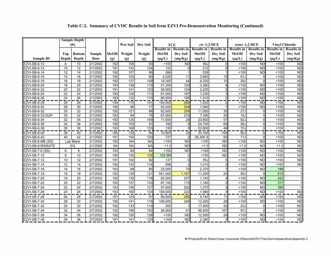
Table C-2. Summary of CVOC Results in Soil from EZVI Pre-Demonstration Monitoring (Continued)

Sample Depth (ft) Wet Soil Dry Soil TCE cis -1,2-DCE trans -1,2-DCE Vinyl Chloride

Sample ID Top

Depth Bottom Depth

Sample Date

MeOH (g)

Weight (g)

Weight (g)

Results in MeOH (µg/L)

Results in Dry Soil (mg/Kg)

Results in MeOH (µg/L)

Results in Dry Soil (mg/Kg)

Results in MeOH (µg/L)

Results in Dry Soil (mg/Kg)

Results in MeOH (µg/L)

Results in Dry Soil (mg/Kg)

EZVI-SB-6-10 8 10 2/1/2002 192 106 93 <100 ND 59J 0 <100 ND <100 ND EZVI-SB-6-12 10 12 2/1/2002 191 142 124 122 0 212 0 <100 ND <100 ND EZVI-SB-6-14 12 14 2/1/2002 192 107 96 266 1 539 1 <100 ND <100 ND EZVI-SB-6-16 14 16 2/1/2002 192 103 90 4,020 11 3,660 10 61J 0 <100 ND EZVI-SB-6-18 16 18 2/1/2002 192 127 109 18,300 44 6,320 15 29J 0 <100 ND EZVI-SB-6-20 18 20 2/1/2002 193 139 115 51,300 120 3,360 8 <100 ND <100 ND EZVI-SB-6-22 20 22 2/1/2002 191 141 123 58,900 124 2,200 5 <100 ND <100 ND EZVI-SB-6-24 22 24 2/1/2002 193 129 113 81,000 187 1,230 3 <100 ND <100 ND EZVI-SB-6-26 24 26 2/1/2002 193 132 110 80,500 195 1,010 2 <100 ND <100 ND EZVI-SB-6-28 26 28 2/1/2002 194 170 141 144,000 280 1,020 2 <100 ND <100 ND EZVI-SB-6-30 28 30 2/1/2002 195 98 77 93,200 324 1,940 7 <100 ND <100 ND EZVI-SB-6-32 30 32 2/1/2002 192 121 88 82,600 259 11,000 35 27J 0 <100 ND EZVI-SB-6-32-DUP 30 32 2/1/2002 193 94 76 67,600 233 7,390 26 16J 0 <100 ND EZVI-SB-6-34 32 34 2/1/2002 192 125 109 11,600 28 23,800 57 62J 0 <100 ND EZVI-SB-6-36 34 36 2/1/2002 190 103 91 169 0 24,700 69 56J 0 <100 ND EZVI-SB-6-38 36 38 2/1/2002 193 168 133 195 0 22,800 48 70J 0 <100 ND EZVI-SB-6-40 38 40 2/1/2002 195 132 94 10,900 33 33,100 100 90J 0 <100 ND EZVI-SB-6-42 40 42 2/1/2002 191 154 120 727 2 26,300 S 60 71J 0 <100 ND EZVI-SB-6-MB (SS) Lab Blank 2/1/2002 192 NA NA <100 ND <100 ND <100 ND <100 ND EZVI-SB-6-RINSATE EQ 2/1/2002 NA NA NA <1.0 ND <1.0 ND <1.0 ND <1.0 ND EZVI-SB-7-8 (SS) 6 8 2/7/2002 193 84 84 <100 ND <100 ND <100 ND <100 ND EZVI-SB-7-10 8 10 2/7/2002 190 135 135 153 SR 0 <100 ND <100 ND <100 ND EZVI-SB-7-12 10 12 2/7/2002 191 102 92 137 0 55J 0 <100 ND <100 ND EZVI-SB-7-14 12 14 2/7/2002 192 133 114 698 2 1,010 2 <100 ND <100 ND EZVI-SB-7-16 14 16 2/7/2002 193 99 85 23,000 70 2,370 7 <100 ND 189 1 EZVI-SB-7-18 16 18 2/7/2002 192 139 121 541,000 1,167 11,200 24 95J 0 615 1 EZVI-SB-7-20 18 20 2/7/2002 192 139 118 92,500 207 1,740 4 <100 ND 422 1 EZVI-SB-7-22 20 22 2/7/2002 192 157 133 87,100 175 1,180 2 <100 ND 317 1 EZVI-SB-7-24 22 24 2/7/2002 193 146 127 97,600 202 1,270 3 <100 ND 390 1 EZVI-SB-7-26 24 26 2/7/2002 193 160 133 109,000 222 1,980 4 <100 ND <100 ND EZVI-SB-7-28 26 28 2/7/2002 191 124 97 96,600 268 4,140 11 <100 ND <100 ND EZVI-SB-7-30 28 30 2/7/2002 195 141 118 109,000 249 12,200 28 <100 ND <100 ND EZVI-SB-7-32 30 32 2/7/2002 192 133 110 305 1 17,400 42 25J 0 <100 ND EZVI-SB-7-34 32 34 2/7/2002 192 198 152 26,900 51 56,500 107 97J 0 <100 ND EZVI-SB-7-36 34 36 2/7/2002 192 150 128 <100 ND 12,500 26 <100 ND <100 ND EZVI-SB-7-38 36 38 2/7/2002 191 141 120 <100 ND 2,380 5 <100 ND <100 ND

M:\Projects\Envir Restor\Cape Canaveral 2\Reports\EZVI Post-Demo\Appendices\Appendix C

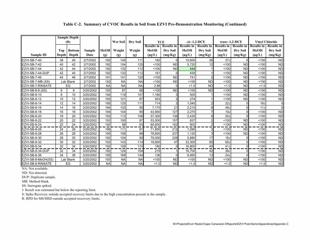
Table C-2. Summary of CVOC Results in Soil from EZVI Pre-Demonstration Monitoring (Continued)

Sample Depth (ft) Wet Soil Dry Soil TCE cis -1,2-DCE trans -1,2-DCE Vinyl Chloride

Sample ID Top

Depth Bottom Depth

Sample Date

MeOH (g)

Weight (g)

Weight (g)

Results in MeOH (µg/L)

Results in Dry Soil (mg/Kg)

Results in MeOH (µg/L)

Results in Dry Soil (mg/Kg)

Results in MeOH (µg/L)

Results in Dry Soil (mg/Kg)

Results in MeOH (µg/L)

Results in Dry Soil (mg/Kg)

EZVI-SB-7-40 38 40 2/7/2002 192 145 111 182 0 10,600 26 37J 0 <100 ND EZVI-SB-7-42 40 42 2/7/2002 192 154 125 <100 ND 5,720 12 <100 ND <100 ND EZVI-SB-7-44 42 44 2/7/2002 192 132 112 <100 ND 444 1 <100 ND <100 ND EZVI-SB-7-44-DUP 42 44 2/7/2002 192 133 112 161 0 430 1 <100 ND <100 ND EZVI-SB-7-46 44 46 2/7/2002 191 141 120 <100 ND 741 2 <100 ND <100 ND EZVI-SB-7-MB (SS) Lab Blank 2/7/2002 192 NA NA <100 ND <100 ND <100 ND <100 ND EZVI-SB-7-RINSATE EQ 2/7/2002 NA NA NA 2.88 0 <1.0 ND <1.0 ND <1.0 ND EZVI-SB-8-8 (SS) 6 8 3/20/2002 193 87 88 <100 ND <100 ND <100 ND <100 ND EZVI-SB-8-10 8 10 3/20/2002 194 119 107 1,180 3 505 1 <100 ND <100 ND EZVI-SB-8-12 10 12 3/20/2002 193 121 87 503 2 274 1 <100 ND <100 ND EZVI-SB-8-14 12 14 3/20/2002 195 125 111 714 2 1,040 2 22J 0 18J 0 EZVI-SB-8-16 14 16 3/20/2002 194 103 90 7,170 21 2,210 6 46J 0 11J 0 EZVI-SB-8-18 16 18 3/20/2002 194 104 90 43,900 127 2,270 7 19J 0 <100 ND EZVI-SB-8-20 18 20 3/20/2002 193 113 106 57,300 136 2,430 6 20J 0 <100 ND EZVI-SB-8-22 20 22 3/20/2002 193 100 87 53,000 157 837 2 <100 ND <100 ND EZVI-SB-8-24 22 24 3/20/2002 192 98 93 60,600 162 802 2 <100 ND <100 ND EZVI-SB-8-26 24 26 3/20/2002 196 111 91 71,800 212 1,090 3 <100 ND <100 ND EZVI-SB-8-28 26 28 3/20/2002 195 106 88 78,800 237 1,120 3 <100 ND <100 ND EZVI-SB-8-30 28 30 3/20/2002 192 104 90 79,000 226 5,880 17 18J 0 <100 ND EZVI-SB-8-32 30 32 3/20/2002 193 143 114 19,600 47 33,300 80 65J 0 <100 ND EZVI-SB-8-34 32 34 3/20/2002 192 126 110 160 0 16,800 40 41J 0 <100 ND EZVI-SB-8-34-DUP 32 34 3/20/2002 192 124 104 219 1 16,700 42 38J 0 <100 ND EZVI-SB-8-36 34 36 3/20/2002 195 169 144 136 0 6,950 13 24J 0 <100 ND EZVI-SB-8-MeOH(SS) Lab Blank 3/20/2002 193 NA NA <100 ND <100 ND <100 ND <100 ND EZVI-SB-8-RINSATE EQ 3/20/2002 NA NA NA <1.0 ND <1.0 ND <1.0 ND <1.0 ND NA: Not available.ND: Not detected.DUP: Duplicate sample.MB: Method blank.SS: Surrogate spiked.J: Result was estimated but below the reporting limit. S: Spike Recovery outside accepted recovery limits due to the high concentration present in the sample. R: RPD for MS/MSD outside accepted receovery limits.

M:\Projects\Envir Restor\Cape Canaveral 2\Reports\EZVI Post-Demo\Appendices\Appendix C

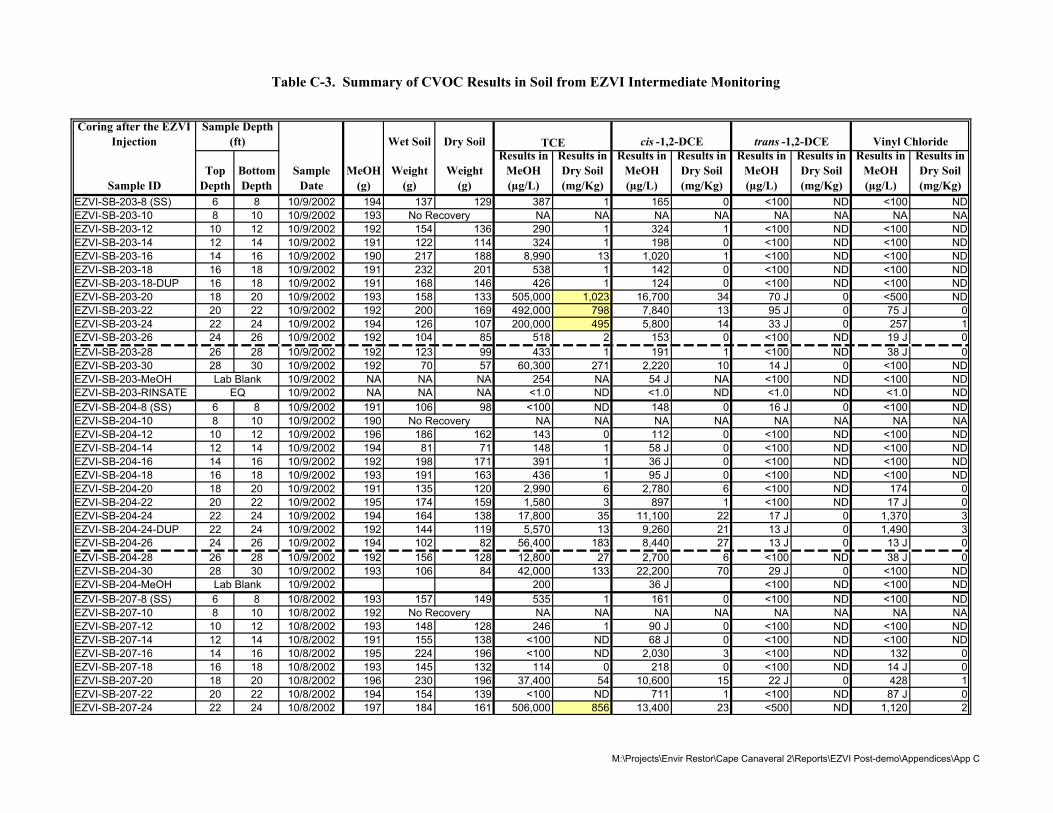
Table C-3. Summary of CVOC Results in Soil from EZVI Intermediate Monitoring

Coring after the EZVI Injection

Sample Depth (ft) Wet Soil Dry Soil TCE cis -1,2-DCE trans -1,2-DCE Vinyl Chloride

Sample ID Top

Depth Bottom Depth

Sample Date

MeOH (g)

Weight (g)

Weight (g)

Results in MeOH (µg/L)

Results in Dry Soil (mg/Kg)

Results in MeOH (µg/L)

Results in Dry Soil (mg/Kg)

Results in MeOH (µg/L)

Results in Dry Soil (mg/Kg)

Results in MeOH (µg/L)

Results in Dry Soil (mg/Kg)

EZVI-SB-203-8 (SS) 6 8 10/9/2002 194 137 129 387 1 165 0 <100 ND <100 ND EZVI-SB-203-10 8 10 10/9/2002 193 No Recovery NA NA NA NA NA NA NA NA EZVI-SB-203-12 10 12 10/9/2002 192 154 136 290 1 324 1 <100 ND <100 ND EZVI-SB-203-14 12 14 10/9/2002 191 122 114 324 1 198 0 <100 ND <100 ND EZVI-SB-203-16 14 16 10/9/2002 190 217 188 8,990 13 1,020 1 <100 ND <100 ND EZVI-SB-203-18 16 18 10/9/2002 191 232 201 538 1 142 0 <100 ND <100 ND EZVI-SB-203-18-DUP 16 18 10/9/2002 191 168 146 426 1 124 0 <100 ND <100 ND EZVI-SB-203-20 18 20 10/9/2002 193 158 133 505,000 1,023 16,700 34 70 J 0 <500 ND EZVI-SB-203-22 20 22 10/9/2002 192 200 169 492,000 798 7,840 13 95 J 0 75 J 0 EZVI-SB-203-24 22 24 10/9/2002 194 126 107 200,000 495 5,800 14 33 J 0 257 1 EZVI-SB-203-26 24 26 10/9/2002 192 104 85 518 2 153 0 <100 ND 19 J 0 EZVI-SB-203-28 26 28 10/9/2002 192 123 99 433 1 191 1 <100 ND 38 J 0 EZVI-SB-203-30 28 30 10/9/2002 192 70 57 60,300 271 2,220 10 14 J 0 <100 ND EZVI-SB-203-MeOH Lab Blank 10/9/2002 NA NA NA 254 NA 54 J NA <100 ND <100 ND EZVI-SB-203-RINSATE EQ 10/9/2002 NA NA NA <1.0 ND <1.0 ND <1.0 ND <1.0 ND EZVI-SB-204-8 (SS) 6 8 10/9/2002 191 106 98 <100 ND 148 0 16 J 0 <100 ND EZVI-SB-204-10 8 10 10/9/2002 190 No Recovery NA NA NA NA NA NA NA NA EZVI-SB-204-12 10 12 10/9/2002 196 186 162 143 0 112 0 <100 ND <100 ND EZVI-SB-204-14 12 14 10/9/2002 194 81 71 148 1 58 J 0 <100 ND <100 ND EZVI-SB-204-16 14 16 10/9/2002 192 198 171 391 1 36 J 0 <100 ND <100 ND EZVI-SB-204-18 16 18 10/9/2002 193 191 163 436 1 95 J 0 <100 ND <100 ND EZVI-SB-204-20 18 20 10/9/2002 191 135 120 2,990 6 2,780 6 <100 ND 174 0 EZVI-SB-204-22 20 22 10/9/2002 195 174 159 1,580 3 897 1 <100 ND 17 J 0 EZVI-SB-204-24 22 24 10/9/2002 194 164 138 17,800 35 11,100 22 17 J 0 1,370 3 EZVI-SB-204-24-DUP 22 24 10/9/2002 192 144 119 5,570 13 9,260 21 13 J 0 1,490 3 EZVI-SB-204-26 24 26 10/9/2002 194 102 82 56,400 183 8,440 27 13 J 0 13 J 0 EZVI-SB-204-28 26 28 10/9/2002 192 156 128 12,800 27 2,700 6 <100 ND 38 J 0 EZVI-SB-204-30 28 30 10/9/2002 193 106 84 42,000 133 22,200 70 29 J 0 <100 ND EZVI-SB-204-MeOH Lab Blank 10/9/2002 200 36 J <100 ND <100 ND EZVI-SB-207-8 (SS) 6 8 10/8/2002 193 157 149 535 1 161 0 <100 ND <100 ND EZVI-SB-207-10 8 10 10/8/2002 192 No Recovery NA NA NA NA NA NA NA NA EZVI-SB-207-12 10 12 10/8/2002 193 148 128 246 1 90 J 0 <100 ND <100 ND EZVI-SB-207-14 12 14 10/8/2002 191 155 138 <100 ND 68 J 0 <100 ND <100 ND EZVI-SB-207-16 14 16 10/8/2002 195 224 196 <100 ND 2,030 3 <100 ND 132 0 EZVI-SB-207-18 16 18 10/8/2002 193 145 132 114 0 218 0 <100 ND 14 J 0 EZVI-SB-207-20 18 20 10/8/2002 196 230 196 37,400 54 10,600 15 22 J 0 428 1 EZVI-SB-207-22 20 22 10/8/2002 194 154 139 <100 ND 711 1 <100 ND 87 J 0 EZVI-SB-207-24 22 24 10/8/2002 197 184 161 506,000 856 13,400 23 <500 ND 1,120 2

M:\Projects\Envir Restor\Cape Canaveral 2\Reports\EZVI Post-demo\Appendices\App C

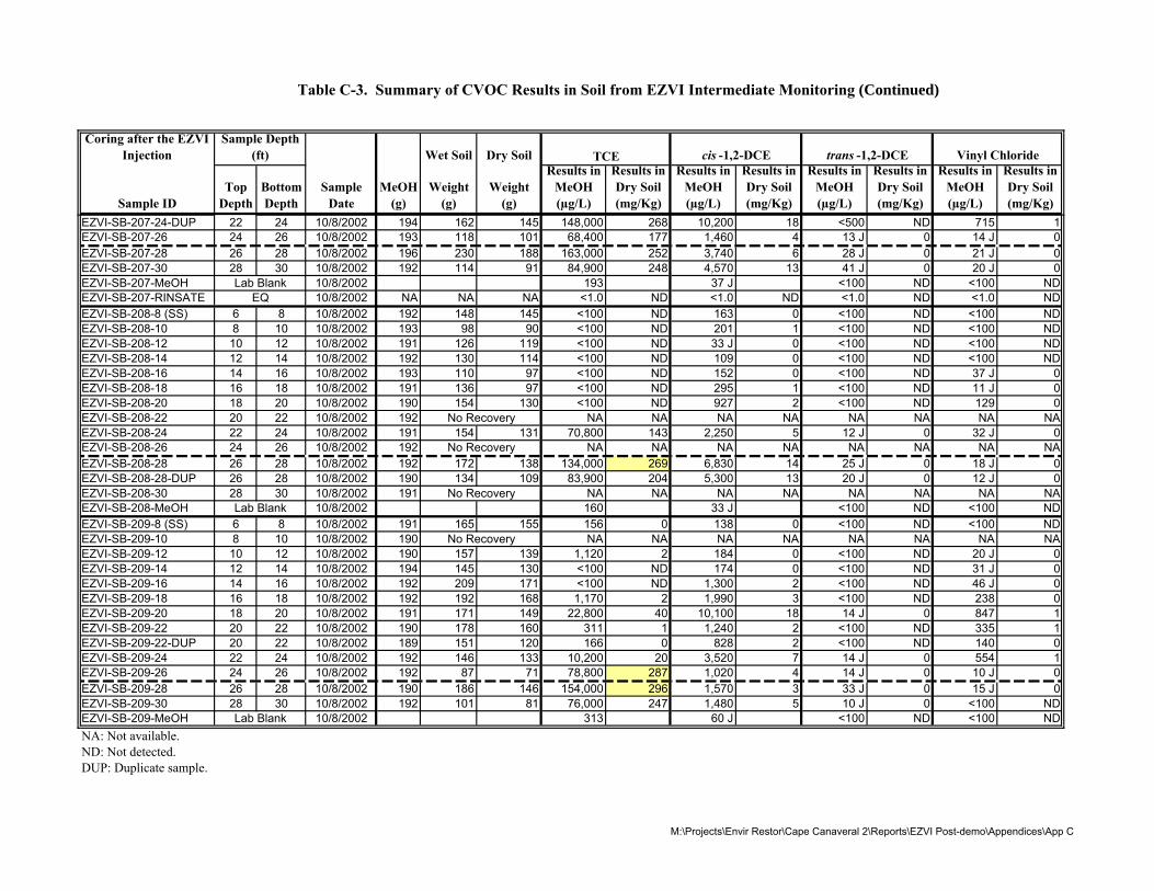
Table C-3. Summary of CVOC Results in Soil from EZVI Intermediate Monitoring (Continued)

Coring after the EZVI Injection

Sample Depth (ft) Wet Soil Dry Soil TCE cis -1,2-DCE trans -1,2-DCE Vinyl Chloride

Sample ID Top

Depth Bottom Depth

Sample Date

MeOH (g)

Weight (g)

Weight (g)

Results in MeOH (µg/L)

Results in Dry Soil (mg/Kg)

Results in MeOH (µg/L)

Results in Dry Soil (mg/Kg)

Results in MeOH (µg/L)

Results in Dry Soil (mg/Kg)

Results in MeOH (µg/L)

Results in Dry Soil (mg/Kg)

EZVI-SB-207-24-DUP 22 24 10/8/2002 194 162 145 148,000 268 10,200 18 <500 ND 715 1 EZVI-SB-207-26 24 26 10/8/2002 193 118 101 68,400 177 1,460 4 13 J 0 14 J 0 EZVI-SB-207-28 26 28 10/8/2002 196 230 188 163,000 252 3,740 6 28 J 0 21 J 0 EZVI-SB-207-30 28 30 10/8/2002 192 114 91 84,900 248 4,570 13 41 J 0 20 J 0 EZVI-SB-207-MeOH Lab Blank 10/8/2002 193 37 J <100 ND <100 ND EZVI-SB-207-RINSATE EQ 10/8/2002 NA NA NA <1.0 ND <1.0 ND <1.0 ND <1.0 ND EZVI-SB-208-8 (SS) 6 8 10/8/2002 192 148 145 <100 ND 163 0 <100 ND <100 ND EZVI-SB-208-10 8 10 10/8/2002 193 98 90 <100 ND 201 1 <100 ND <100 ND EZVI-SB-208-12 10 12 10/8/2002 191 126 119 <100 ND 33 J 0 <100 ND <100 ND EZVI-SB-208-14 12 14 10/8/2002 192 130 114 <100 ND 109 0 <100 ND <100 ND EZVI-SB-208-16 14 16 10/8/2002 193 110 97 <100 ND 152 0 <100 ND 37 J 0 EZVI-SB-208-18 16 18 10/8/2002 191 136 97 <100 ND 295 1 <100 ND 11 J 0 EZVI-SB-208-20 18 20 10/8/2002 190 154 130 <100 ND 927 2 <100 ND 129 0 EZVI-SB-208-22 20 22 10/8/2002 192 No Recovery NA NA NA NA NA NA NA NA EZVI-SB-208-24 22 24 10/8/2002 191 154 131 70,800 143 2,250 5 12 J 0 32 J 0 EZVI-SB-208-26 24 26 10/8/2002 192 No Recovery NA NA NA NA NA NA NA NA EZVI-SB-208-28 26 28 10/8/2002 192 172 138 134,000 269 6,830 14 25 J 0 18 J 0 EZVI-SB-208-28-DUP 26 28 10/8/2002 190 134 109 83,900 204 5,300 13 20 J 0 12 J 0 EZVI-SB-208-30 28 30 10/8/2002 191 No Recovery NA NA NA NA NA NA NA NA EZVI-SB-208-MeOH Lab Blank 10/8/2002 160 33 J <100 ND <100 ND EZVI-SB-209-8 (SS) 6 8 10/8/2002 191 165 155 156 0 138 0 <100 ND <100 ND EZVI-SB-209-10 8 10 10/8/2002 190 No Recovery NA NA NA NA NA NA NA NA EZVI-SB-209-12 10 12 10/8/2002 190 157 139 1,120 2 184 0 <100 ND 20 J 0 EZVI-SB-209-14 12 14 10/8/2002 194 145 130 <100 ND 174 0 <100 ND 31 J 0 EZVI-SB-209-16 14 16 10/8/2002 192 209 171 <100 ND 1,300 2 <100 ND 46 J 0 EZVI-SB-209-18 16 18 10/8/2002 192 192 168 1,170 2 1,990 3 <100 ND 238 0 EZVI-SB-209-20 18 20 10/8/2002 191 171 149 22,800 40 10,100 18 14 J 0 847 1 EZVI-SB-209-22 20 22 10/8/2002 190 178 160 311 1 1,240 2 <100 ND 335 1 EZVI-SB-209-22-DUP 20 22 10/8/2002 189 151 120 166 0 828 2 <100 ND 140 0 EZVI-SB-209-24 22 24 10/8/2002 192 146 133 10,200 20 3,520 7 14 J 0 554 1 EZVI-SB-209-26 24 26 10/8/2002 192 87 71 78,800 287 1,020 4 14 J 0 10 J 0 EZVI-SB-209-28 26 28 10/8/2002 190 186 146 154,000 296 1,570 3 33 J 0 15 J 0 EZVI-SB-209-30 28 30 10/8/2002 192 101 81 76,000 247 1,480 5 10 J 0 <100 ND EZVI-SB-209-MeOH Lab Blank 10/8/2002 313 60 J <100 ND <100 ND NA: Not available.ND: Not detected.DUP: Duplicate sample.

M:\Projects\Envir Restor\Cape Canaveral 2\Reports\EZVI Post-demo\Appendices\App C

Coring after the EZVI Sample Depth Injection (ft) Wet Soil Dry Soil TCE cis -1,2-DCE trans -1,2-DCE Vinyl Chloride

Results in Results in Results in Results in Results in Results in Results in Results in Top Bottom Sample MeOH Weight Weight MeOH Dry Soil MeOH Dry Soil MeOH Dry Soil MeOH Dry Soil

Sample ID Depth Depth Date (g) (g) (g) (µg/L) (mg/Kg) (µg/L) (mg/Kg) (µg/L) (mg/Kg) (µg/L) (mg/Kg)

Table C-3. Summary of CVOC Results in Soil from EZVI Intermediate Monitoring (Continued)

MB: Method blank. SS: Surrogate spiked. J: Result was estimated but below the reporting limit. S: Spike Recovery outside accepted recovery limits due to the high concentration present in the sample. R: RPD for MS/MSD outside accepted receovery limits.

M:\Projects\Envir Restor\Cape Canaveral 2\Reports\EZVI Post-demo\Appendices\App C

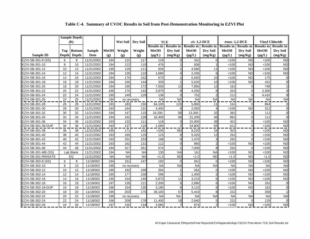
Table C-4. Summary of CVOC Results in Soil from Post-Demonstration Monitoring in EZVI Plot

Sample Depth (ft) Wet Soil Dry Soil TCE cis -1,2-DCE trans -1,2-DCE Vinyl Chloride

Sample ID Top

Depth Bottom Depth

Sample Date

MeOH (g)

Weight (g)

Weight (g)

Results in MeOH (µg/L)

Results in Dry Soil (mg/Kg)

Results in MeOH (µg/L)

Results in Dry Soil (mg/Kg)

Results in MeOH (µg/L)

Results in Dry Soil (mg/Kg)

Results in MeOH (µg/L)

Results in Dry Soil (mg/Kg)

EZVI-SB-301-8 (SS) 6 8 11/21/2002 194 122 117 119 0 33J 0 <100 ND <100 ND EZVI-SB-301-10 8 10 11/21/2002 194 122 110 476 1 506 1 <100 ND <100 ND EZVI-SB-301-12 10 12 11/21/2002 195 129 111 626 1 4,580 11 <100 ND <100 ND EZVI-SB-301-14 12 14 11/21/2002 194 130 110 1,680 4 2,430 6 <100 ND <100 ND EZVI-SB-301-16 14 16 11/21/2002 194 170 152 670 1 5,560 10 <100 ND 175 0 EZVI-SB-301-18 16 18 11/21/2002 194 165 144 329 1 5,520 10 <100 ND 43J 0 EZVI-SB-301-20 18 20 11/21/2002 194 195 172 7,500 12 7,850 12 16J 0 748 1 EZVI-SB-301-22 20 22 11/21/2002 195 170 142 3,970 8 4,250 8 20J 0 2,300 4 EZVI-SB-301-24 22 24 11/21/2002 195 149 129 136 0 752 2 21J 0 4,410 9 EZVI-SB-301-26 24 26 11/21/2002 194 no recovery NA NA NA NA NA NA NA NA EZVI-SB-301-28 26 28 11/21/2002 193 183 150 64,100 119 5,860 11 16J 0 864 2 EZVI-SB-301-30 28 30 11/21/2002 193 164 131 4,450 9 2,050 4 <100 ND 52J 0 EZVI-SB-301-32 30 32 11/21/2002 194 147 115 24,200 58 13,300 32 38J 0 11J 0 EZVI-SB-301-34 32 34 11/21/2002 194 162 128 16,400 36 21,200 46 88J 0 11J 0 EZVI-SB-301-36 34 36 11/21/2002 193 132 111 118 0 15,900 38 40J 0 <100 ND EZVI-SB-301-36-DUP 34 36 11/21/2002 193 137 119 1,090 2 24,800 55 61J 0 <100 ND EZVI-SB-301-38 36 38 11/21/2002 195 171 142 <100 ND 8,220 16 30J 0 <100 ND EZVI-SB-301-40 38 40 11/21/2002 193 165 120 123 0 5,020 12 26J 0 <100 ND EZVI-SB-301-42 40 42 11/21/2002 193 201 153 168 0 1,470 3 28J 0 <100 ND EZVI-SB-301-44 42 44 11/21/2002 193 162 131 112 0 860 2 <100 ND <100 ND EZVI-SB-301-46 44 46 11/21/2002 194 317 261 574 1 7,000 8 29J 0 <100 ND EZVI-SB-301-MB (SS) Lab Blank 11/21/2002 194 NA NA 130 NA 16J NA <100 ND <100 ND EZVI-SB-301-RINSATE EQ 11/21/2002 NA NA NA <1.0 ND <1.0 ND <1.0 ND <1.0 ND EZVI-SB-302-8 (SS) 6 8 11/18/002 194 151 147 192 0 65J 0 <100 ND <100 ND EZVI-SB-302-10 8 10 11/18/002 195 no recovery NA NA NA NA NA NA NA NA EZVI-SB-302-12 10 12 11/18/002 195 192 168 354 1 262 0 <100 ND <100 ND EZVI-SB-302-14 12 14 11/18/002 195 177 158 596 1 1,400 2 <100 ND <100 ND EZVI-SB-302-16 14 16 11/18/002 195 154 140 5,870 11 3,210 6 <100 ND <100 ND EZVI-SB-302-18 16 18 11/18/002 197 135 121 2,330 5 2,890 6 <100 ND 26J 0 EZVI-SB-302-18-DUP 16 18 11/18/002 196 154 135 3,180 6 3,110 6 <100 ND 18J 0 EZVI-SB-302-20 18 20 11/18/002 195 203 175 36,100 57 5,410 8 23J 0 358 1 EZVI-SB-302-22 20 22 11/18/002 196 no recovery NA NA NA NA NA NA NA NA EZVI-SB-302-24 22 24 11/18/002 196 209 178 11,400 18 2,940 5 23J 0 129 0 EZVI-SB-302-26 24 26 11/18/002 197 155 134 3,680 7 974 2 <100 ND <100 ND

M:\Cape Canaveral 2\Reports\Final Reports\EZVI\Appendix\App C\EZVI Post-demo TCE Soil Results.xls

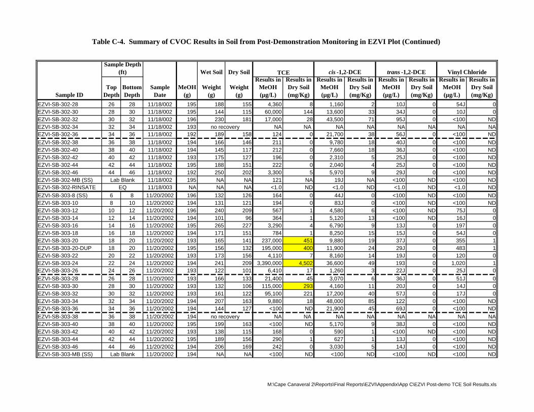
Table C-4. Summary of CVOC Results in Soil from Post-Demonstration Monitoring in EZVI Plot (Continued)

Sample Depth (ft) Wet Soil Dry Soil TCE cis -1,2-DCE trans -1,2-DCE Vinyl Chloride

Sample ID Top

Depth Bottom Depth

Sample Date

MeOH (g)

Weight (g)

Weight (g)

Results in MeOH (µg/L)

Results in Dry Soil (mg/Kg)

Results in MeOH (µg/L)

Results in Dry Soil (mg/Kg)

Results in MeOH (µg/L)

Results in Dry Soil (mg/Kg)

Results in MeOH (µg/L)

Results in Dry Soil (mg/Kg)

EZVI-SB-302-28 26 28 11/18/002 195 188 155 4,360 8 1,160 2 10J 0 54J 0 EZVI-SB-302-30 28 30 11/18/002 195 144 115 60,000 144 13,600 33 34J 0 10J 0 EZVI-SB-302-32 30 32 11/18/002 196 230 181 17,000 28 43,500 71 95J 0 <100 ND EZVI-SB-302-34 32 34 11/18/002 193 no recovery NA NA NA NA NA NA NA NA EZVI-SB-302-36 34 36 11/18/002 192 189 158 124 0 21,700 38 56J 0 <100 ND EZVI-SB-302-38 36 38 11/18/002 194 166 146 211 0 9,780 18 40J 0 <100 ND EZVI-SB-302-40 38 40 11/18/002 194 145 117 212 0 7,660 18 36J 0 <100 ND EZVI-SB-302-42 40 42 11/18/002 193 175 127 196 0 2,310 5 25J 0 <100 ND EZVI-SB-302-44 42 44 11/18/002 195 188 151 222 0 2,040 4 25J 0 <100 ND EZVI-SB-302-46 44 46 11/18/002 192 250 202 3,300 5 5,970 9 29J 0 <100 ND EZVI-SB-302-MB (SS) Lab Blank 11/18/002 195 NA NA 121 NA 19J NA <100 ND <100 ND EZVI-SB-302-RINSATE EQ 11/18/003 NA NA NA <1.0 ND <1.0 ND <1.0 ND <1.0 ND EZVI-SB-303-8 (SS) 6 8 11/20/2002 196 132 126 164 0 44J 0 <100 ND <100 ND EZVI-SB-303-10 8 10 11/20/2002 194 131 121 194 0 83J 0 <100 ND <100 ND EZVI-SB-303-12 10 12 11/20/2002 196 240 209 567 1 4,580 6 <100 ND 75J 0 EZVI-SB-303-14 12 14 11/20/2002 194 101 96 364 1 5,120 13 <100 ND 16J 0 EZVI-SB-303-16 14 16 11/20/2002 195 265 227 3,290 4 6,790 9 13J 0 197 0 EZVI-SB-303-18 16 18 11/20/2002 194 171 151 784 1 8,250 15 15J 0 54J 0 EZVI-SB-303-20 18 20 11/20/2002 193 165 141 237,000 451 9,880 19 37J 0 355 1 EZVI-SB-303-20-DUP 18 20 11/20/2002 195 156 132 195,000 400 11,900 24 29J 0 483 1 EZVI-SB-303-22 20 22 11/20/2002 193 173 156 4,110 7 8,160 14 19J 0 120 0 EZVI-SB-303-24 22 24 11/20/2002 194 241 209 3,390,000 4,502 36,600 49 193 0 1,020 1 EZVI-SB-303-26 24 26 11/20/2002 193 122 101 6,410 17 1,260 3 22J 0 25J 0 EZVI-SB-303-28 26 28 11/20/2002 193 166 133 21,400 45 3,070 6 36J 0 51J 0 EZVI-SB-303-30 28 30 11/20/2002 193 132 106 115,000 293 4,160 11 20J 0 14J 0 EZVI-SB-303-32 30 32 11/20/2002 193 161 122 95,100 221 17,200 40 57J 0 17J 0 EZVI-SB-303-34 32 34 11/20/2002 194 207 163 9,880 18 48,000 85 122 0 <100 ND EZVI-SB-303-36 34 36 11/20/2002 194 144 127 <100 ND 21,900 45 69J 0 <100 ND EZVI-SB-303-38 36 38 11/20/2002 194 no recovery NA NA NA NA NA NA NA NA EZVI-SB-303-40 38 40 11/20/2002 195 199 163 <100 ND 5,170 9 38J 0 <100 ND EZVI-SB-303-42 40 42 11/20/2002 193 138 115 168 0 590 1 <100 ND <100 ND EZVI-SB-303-44 42 44 11/20/2002 195 189 156 290 1 627 1 13J 0 <100 ND EZVI-SB-303-46 44 46 11/20/2002 194 206 169 242 0 3,030 5 14J 0 <100 ND EZVI-SB-303-MB (SS) Lab Blank 11/20/2002 194 NA NA <100 ND <100 ND <100 ND <100 ND

M:\Cape Canaveral 2\Reports\Final Reports\EZVI\Appendix\App C\EZVI Post-demo TCE Soil Results.xls

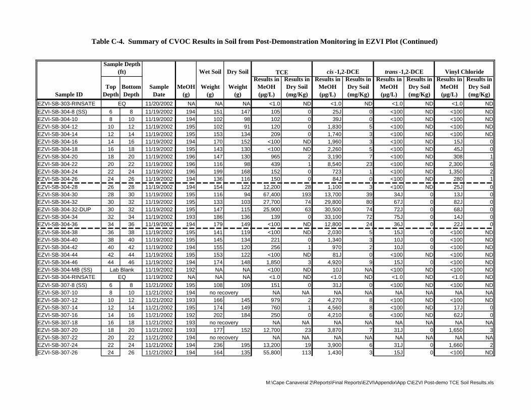
Table C-4. Summary of CVOC Results in Soil from Post-Demonstration Monitoring in EZVI Plot (Continued)

Sample Depth (ft) Wet Soil Dry Soil TCE cis -1,2-DCE trans -1,2-DCE Vinyl Chloride

Sample ID Top

Depth Bottom Depth

Sample Date

MeOH (g)

Weight (g)

Weight (g)

Results in MeOH (µg/L)

Results in Dry Soil (mg/Kg)

Results in MeOH (µg/L)

Results in Dry Soil (mg/Kg)

Results in MeOH (µg/L)

Results in Dry Soil (mg/Kg)

Results in MeOH (µg/L)

Results in Dry Soil (mg/Kg)

EZVI-SB-303-RINSATE EQ 11/20/2002 NA NA NA <1.0 ND <1.0 ND <1.0 ND <1.0 ND EZVI-SB-304-8 (SS) 6 8 11/19/2002 194 151 147 105 0 25J 0 <100 ND <100 ND EZVI-SB-304-10 8 10 11/19/2002 194 102 98 102 0 39J 0 <100 ND <100 ND EZVI-SB-304-12 10 12 11/19/2002 195 102 91 120 0 1,830 5 <100 ND <100 ND EZVI-SB-304-14 12 14 11/19/2002 195 153 134 209 0 1,740 3 <100 ND <100 ND EZVI-SB-304-16 14 16 11/19/2002 194 170 152 <100 ND 1,960 3 <100 ND 15J 0 EZVI-SB-304-18 16 18 11/19/2002 195 143 130 <100 ND 2,260 5 <100 ND 45J 0 EZVI-SB-304-20 18 20 11/19/2002 196 147 130 965 2 3,190 7 <100 ND 308 1 EZVI-SB-304-22 20 22 11/19/2002 196 116 98 439 1 8,540 23 <100 ND 2,300 6 EZVI-SB-304-24 22 24 11/19/2002 196 199 168 152 0 723 1 <100 ND 1,350 2 EZVI-SB-304-26 24 26 11/19/2002 194 136 116 150 0 84J 0 <100 ND 280 1 EZVI-SB-304-28 26 28 11/19/2002 194 154 122 12,200 28 1,100 3 <100 ND 25J 0 EZVI-SB-304-30 28 30 11/19/2002 195 116 94 67,400 193 13,700 39 34J 0 13J 0 EZVI-SB-304-32 30 32 11/19/2002 195 133 103 27,700 74 29,800 80 67J 0 82J 0 EZVI-SB-304-32-DUP 30 32 11/19/2002 195 147 115 25,900 63 30,500 74 72J 0 68J 0 EZVI-SB-304-34 32 34 11/19/2002 193 186 136 139 0 33,100 72 75J 0 14J 0 EZVI-SB-304-36 34 36 11/19/2002 194 179 149 <100 ND 12,800 24 36J 0 22J 0 EZVI-SB-304-38 36 38 11/19/2002 195 141 119 <100 ND 2,030 5 15J 0 <100 ND EZVI-SB-304-40 38 40 11/19/2002 195 145 134 221 0 1,340 3 10J 0 <100 ND EZVI-SB-304-42 40 42 11/19/2002 194 155 120 256 1 970 2 10J 0 <100 ND EZVI-SB-304-44 42 44 11/19/2002 195 153 122 <100 ND 81J 0 <100 ND <100 ND EZVI-SB-304-46 44 46 11/19/2002 194 174 148 1,850 3 4,920 9 15J 0 <100 ND EZVI-SB-304-MB (SS) Lab Blank 11/19/2002 192 NA NA <100 ND 10J NA <100 ND <100 ND EZVI-SB-304-RINSATE EQ 11/19/2002 NA NA NA <1.0 ND <1.0 ND <1.0 ND <1.0 ND EZVI-SB-307-8 (SS) 6 8 11/21/2002 195 108 109 151 0 31J 0 <100 ND <100 ND EZVI-SB-307-10 8 10 11/21/2002 194 no recovery NA NA NA NA NA NA NA NA EZVI-SB-307-12 10 12 11/21/2002 193 166 145 979 2 4,270 8 <100 ND <100 ND EZVI-SB-307-14 12 14 11/21/2002 195 174 149 760 1 4,560 8 <100 ND 17J 0 EZVI-SB-307-16 14 16 11/21/2002 192 202 184 250 0 4,210 6 <100 ND 62J 0 EZVI-SB-307-18 16 18 11/21/2002 193 no recovery NA NA NA NA NA NA NA NA EZVI-SB-307-20 18 20 11/21/2002 193 177 152 12,700 23 3,870 7 31J 0 1,650 3 EZVI-SB-307-22 20 22 11/21/2002 194 no recovery NA NA NA NA NA NA NA NA EZVI-SB-307-24 22 24 11/21/2002 194 236 195 13,200 19 3,900 6 31J 0 1,660 2 EZVI-SB-307-26 24 26 11/21/2002 194 164 135 55,800 113 1,430 3 15J 0 <100 ND

M:\Cape Canaveral 2\Reports\Final Reports\EZVI\Appendix\App C\EZVI Post-demo TCE Soil Results.xls

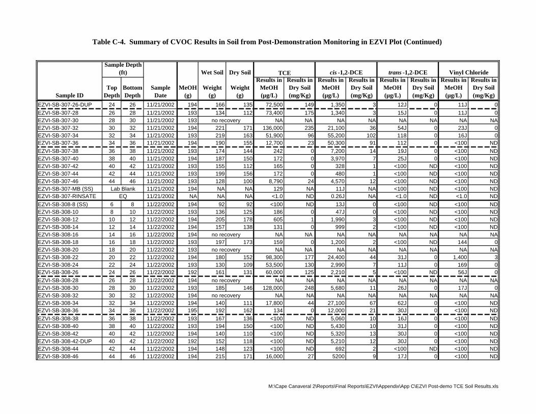
Table C-4. Summary of CVOC Results in Soil from Post-Demonstration Monitoring in EZVI Plot (Continued)

Sample Depth (ft) Wet Soil Dry Soil TCE cis -1,2-DCE trans -1,2-DCE Vinyl Chloride

Sample ID Top

Depth Bottom Depth

Sample Date

MeOH (g)

Weight (g)

Weight (g)

Results in MeOH (µg/L)

Results in Dry Soil (mg/Kg)

Results in MeOH (µg/L)

Results in Dry Soil (mg/Kg)

Results in MeOH (µg/L)

Results in Dry Soil (mg/Kg)

Results in MeOH (µg/L)

Results in Dry Soil (mg/Kg)

EZVI-SB-307-26-DUP 24 26 11/21/2002 194 166 135 72,500 149 1,350 3 12J 0 11J 0 EZVI-SB-307-28 26 28 11/21/2002 193 134 112 73,400 175 1,340 3 15J 0 11J 0 EZVI-SB-307-30 28 30 11/21/2002 193 no recovery NA NA NA NA NA NA NA NA EZVI-SB-307-32 30 32 11/21/2002 194 221 171 136,000 235 21,100 36 54J 0 23J 0 EZVI-SB-307-34 32 34 11/21/2002 193 219 163 51,900 96 55,200 102 118 0 16J 0 EZVI-SB-307-36 34 36 11/21/2002 194 190 155 12,700 23 50,300 91 112 0 <100 ND EZVI-SB-307-38 36 38 11/21/2002 193 174 144 242 0 7,200 14 19J 0 <100 ND EZVI-SB-307-40 38 40 11/21/2002 194 187 150 172 0 3,970 7 25J 0 <100 ND EZVI-SB-307-42 40 42 11/21/2002 193 155 112 165 0 328 1 <100 ND <100 ND EZVI-SB-307-44 42 44 11/21/2002 193 199 156 172 0 480 1 <100 ND <100 ND EZVI-SB-307-46 44 46 11/21/2002 193 128 100 8,790 24 4,570 12 <100 ND <100 ND EZVI-SB-307-MB (SS) Lab Blank 11/21/2002 194 NA NA 129 NA 11J NA <100 ND <100 ND EZVI-SB-307-RINSATE EQ 11/21/2002 NA NA NA <1.0 ND 0.26J NA <1.0 ND <1.0 ND EZVI-SB-308-8 (SS) 6 8 11/22/2002 194 92 92 <100 ND 13J 0 <100 ND <100 ND EZVI-SB-308-10 8 10 11/22/2002 193 136 125 186 0 47J 0 <100 ND <100 ND EZVI-SB-308-12 10 12 11/22/2002 194 205 178 605 1 1,990 3 <100 ND <100 ND EZVI-SB-308-14 12 14 11/22/2002 194 157 138 131 0 999 2 <100 ND <100 ND EZVI-SB-308-16 14 16 11/22/2002 194 no recovery NA NA NA NA NA NA NA NA EZVI-SB-308-18 16 18 11/22/2002 193 197 173 159 0 1,200 2 <100 ND 144 0 EZVI-SB-308-20 18 20 11/22/2002 193 no recovery NA NA NA NA NA NA NA NA EZVI-SB-308-22 20 22 11/22/2002 194 180 152 98,300 177 24,400 44 31J 0 1,400 3 EZVI-SB-308-24 22 24 11/22/2002 193 130 109 53,500 130 2,990 7 11J 0 169 0 EZVI-SB-308-26 24 26 11/22/2002 192 161 131 60,000 125 2,210 5 <100 ND 56J 0 EZVI-SB-308-28 26 28 11/22/2002 194 no recovery NA NA NA NA NA NA NA NA EZVI-SB-308-30 28 30 11/22/2002 193 185 146 128,000 248 5,680 11 26J 0 17J 0 EZVI-SB-308-32 30 32 11/22/2002 194 no recovery NA NA NA NA NA NA NA NA EZVI-SB-308-34 32 34 11/22/2002 194 140 111 17,800 44 27,100 67 62J 0 <100 ND EZVI-SB-308-36 34 36 11/22/2002 195 192 162 134 0 12,000 21 30J 0 <100 ND EZVI-SB-308-38 36 38 11/22/2002 193 167 136 <100 ND 5,060 10 16J 0 <100 ND EZVI-SB-308-40 38 40 11/22/2002 193 194 150 <100 ND 5,430 10 31J 0 <100 ND EZVI-SB-308-42 40 42 11/22/2002 194 140 110 <100 ND 5,320 13 30J 0 <100 ND EZVI-SB-308-42-DUP 40 42 11/22/2002 192 152 118 <100 ND 5,210 12 30J 0 <100 ND EZVI-SB-308-44 42 44 11/22/2002 194 148 123 <100 ND 692 2 <100 ND <100 ND EZVI-SB-308-46 44 46 11/22/2002 194 215 171 16,000 27 5200 9 17J 0 <100 ND

M:\Cape Canaveral 2\Reports\Final Reports\EZVI\Appendix\App C\EZVI Post-demo TCE Soil Results.xls

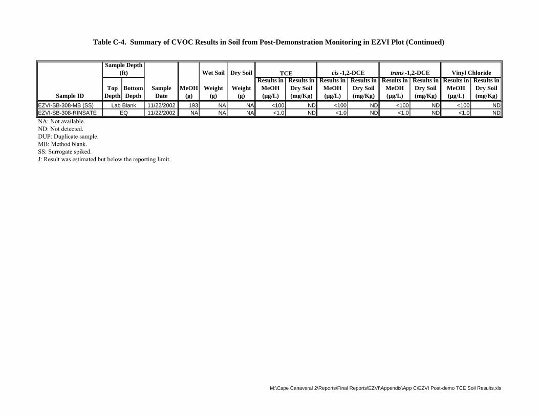
Table C-4. Summary of CVOC Results in Soil from Post-Demonstration Monitoring in EZVI Plot (Continued)

Sample Depth (ft) Wet Soil Dry Soil TCE cis -1,2-DCE trans -1,2-DCE Vinyl Chloride

Results in Results in Results in Results in Results in Results in Results in Results in Top Bottom Sample MeOH Weight Weight MeOH Dry Soil MeOH Dry Soil MeOH Dry Soil MeOH Dry Soil

Sample ID Depth Depth Date (g) (g) (g) (µg/L) (mg/Kg) (µg/L) (mg/Kg) (µg/L) (mg/Kg) (µg/L) (mg/Kg) EZVI-SB-308-MB (SS) Lab Blank 11/22/2002 193 NA NA <100 ND <100 ND <100 ND <100 ND EZVI-SB-308-RINSATE EQ 11/22/2002 NA NA NA <1.0 ND <1.0 ND <1.0 ND <1.0 ND NA: Not available.ND: Not detected.DUP: Duplicate sample.MB: Method blank.SS: Surrogate spiked.J: Result was estimated but below the reporting limit.

M:\Cape Canaveral 2\Reports\Final Reports\EZVI\Appendix\App C\EZVI Post-demo TCE Soil Results.xls

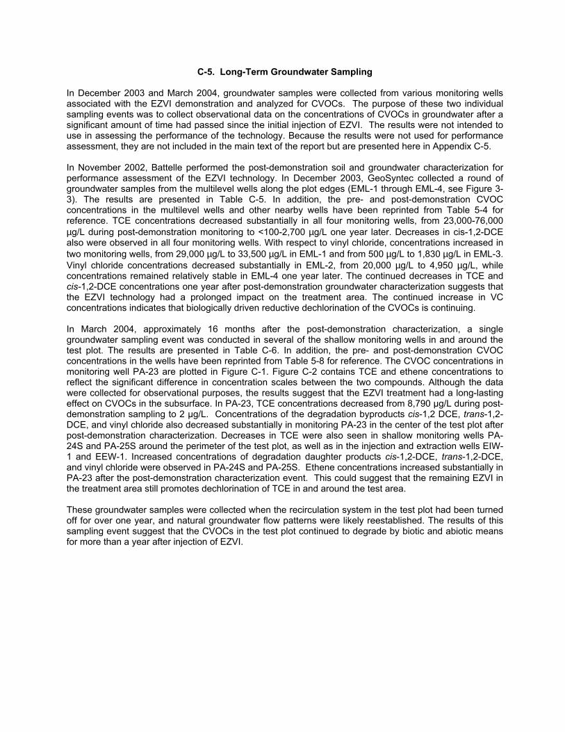
C-5. Long-Term Groundwater Sampling

In December 2003 and March 2004, groundwater samples were collected from various monitoring wells associated with the EZVI demonstration and analyzed for CVOCs. The purpose of these two individual sampling events was to collect observational data on the concentrations of CVOCs in groundwater after a significant amount of time had passed since the initial injection of EZVI. The results were not intended to use in assessing the performance of the technology. Because the results were not used for performance assessment, they are not included in the main text of the report but are presented here in Appendix C-5.

In November 2002, Battelle performed the post-demonstration soil and groundwater characterization for performance assessment of the EZVI technology. In December 2003, GeoSyntec collected a round of groundwater samples from the multilevel wells along the plot edges (EML-1 through EML-4, see Figure 3­3). The results are presented in Table C-5. In addition, the pre- and post-demonstration CVOC concentrations in the multilevel wells and other nearby wells have been reprinted from Table 5-4 for reference. TCE concentrations decreased substantially in all four monitoring wells, from 23,000-76,000 µg/L during post-demonstration monitoring to <100-2,700 µg/L one year later. Decreases in cis-1,2-DCE also were observed in all four monitoring wells. With respect to vinyl chloride, concentrations increased in two monitoring wells, from 29,000 µg/L to 33,500 µg/L in EML-1 and from 500 µg/L to 1,830 µg/L in EML-3. Vinyl chloride concentrations decreased substantially in EML-2, from 20,000 µg/L to 4,950 µg/L, while concentrations remained relatively stable in EML-4 one year later. The continued decreases in TCE and cis-1,2-DCE concentrations one year after post-demonstration groundwater characterization suggests that the EZVI technology had a prolonged impact on the treatment area. The continued increase in VC concentrations indicates that biologically driven reductive dechlorination of the CVOCs is continuing.

In March 2004, approximately 16 months after the post-demonstration characterization, a single groundwater sampling event was conducted in several of the shallow monitoring wells in and around the test plot. The results are presented in Table C-6. In addition, the pre- and post-demonstration CVOC concentrations in the wells have been reprinted from Table 5-8 for reference. The CVOC concentrations in monitoring well PA-23 are plotted in Figure C-1. Figure C-2 contains TCE and ethene concentrations to reflect the significant difference in concentration scales between the two compounds. Although the data were collected for observational purposes, the results suggest that the EZVI treatment had a long-lasting effect on CVOCs in the subsurface. In PA-23, TCE concentrations decreased from 8,790 µg/L during post-demonstration sampling to 2 µg/L. Concentrations of the degradation byproducts cis-1,2 DCE, trans-1,2­DCE, and vinyl chloride also decreased substantially in monitoring PA-23 in the center of the test plot after post-demonstration characterization. Decreases in TCE were also seen in shallow monitoring wells PA­24S and PA-25S around the perimeter of the test plot, as well as in the injection and extraction wells EIW­1 and EEW-1. Increased concentrations of degradation daughter products cis-1,2-DCE, trans-1,2-DCE, and vinyl chloride were observed in PA-24S and PA-25S. Ethene concentrations increased substantially in PA-23 after the post-demonstration characterization event. This could suggest that the remaining EZVI in the treatment area still promotes dechlorination of TCE in and around the test area.

These groundwater samples were collected when the recirculation system in the test plot had been turned off for over one year, and natural groundwater flow patterns were likely reestablished. The results of this sampling event suggest that the CVOCs in the test plot continued to degrade by biotic and abiotic means for more than a year after injection of EZVI.

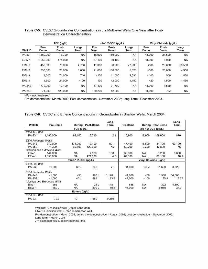
Well ID

TCE (µg/L) cis-1,2-DCE (µg/L) Vinyl Chloride (µg/L) Pre-

Demo Post-Demo

Long-Term

Pre-Demo

Post-Demo

Long-Term

Pre-Demo

Post-Demo

Long-Term

PA-23 1,180,000 8,790 NA 16,900 169,000 NA <1,000 21,600 NA

EEW-1 1,050,000 471,000 NA 67,100 80,100 NA <1,000 6,980 NA

EML-1 450,000 76,000 2,700 11,000 96,000 77,900 <500 29,000 33,500

EML-2 350,000 23,000 1,000 21,000 130,000 5,320 <500 20,000 4,950

EML-3 1,300 74,000 740 <100 41,000 2,630 <100 500 1,830

EML-4 1,600 24,000 <100 130 42,000 1,150 <20 1,500 1,460

PA-24S 772,000 12,100 NA 47,400 31,700 NA <1,000 1,580 NA

PA-25S 71,300 129,000 NA 69,200 42,800 NA <1,000 75J NA

NA = not analyzed Pre-demonstration: March 2002; Post-demonstration: November 2002; Long-Term: December 2003.

Well ID Pre-Demo During Post-Demo Long-Term Pre-Demo During Post-Demo

Long-Term

TCE (µg/L) cis-1,2-DCE (µg/L) EZVI Plot Well

PA-23 1,180,000 92,100 8,790 2 J 16,900 17,900 169,000 870

EZVI Perimeter Wells PA-24S 772,000 474,000 12,100 501 47,400 15,800 31,700 63,100 PA-25S 71,300 69,600 129,000 <5 69,200 9,320 42,800 <5

Injection and Extraction Wells EIW-1 144,000 NA 7,820 108 38,300 NA 3,280 8,650 EEW-1 1,050,000 NA 471,000 4.5 67,100 NA 80,100 10.6

trans-1,2-DCE (µg/L) Vinyl Chloride (µg/L) EZVI Plot Well

PA-23 <1,000 68 J 245 71 <1,000 53 J 21,600 3,620

EZVI Perimeter Wells PA-24S <1,000 <50 190 J 1,140 <1,000 <50 1,580 54,600 PA-25S <1,000 46 J 381 83.8 <1,000 <100 75 J 8.75

Injection and Extraction Wells EIW-1 556 NA 24 J 148 638 NA 322 4,890 EEW-1 550 J NA 390 J 10.5 <1,000 NA 6,980 34.9

Ethene (µg/L) EZVI Plot Well

PA-23 79.3 10 1,680 9,280

Well IDs: S = shallow well (Upper Sand Unit) EIW-1 = injection well; EEW-1 = extraction well. Pre-demonstration = March 2002; during the demonstration = August 2002; post-demonstration = November 2002; Long-term = March 2004 J = Estimated value, below reporting limit.

Table C-5. CVOC Groundwater Concentrations in the Multilevel Wells One Year after Post-Demonstration Characterization

Table C-6. CVOC and Ethene Concentrations in Groundwater in Shallow Wells, March 2004

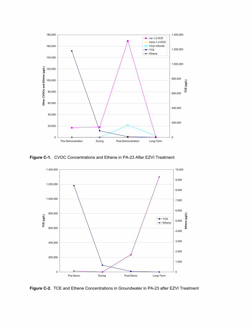
0

20,000

40,000

60,000

80,000

100,000

120,000

140,000

160,000

180,000

Oth

er C

VOC

s an

d Et

hene

(µg/

L)

0

200,000

400,000

600,000

800,000

1,000,000

1,200,000

1,400,000

TCE

(µg/

L)

cis-1,2-DCE trans-1,2-DCE Vinyl chloride TCE Ethene

Pre-Demonstration During Post-Demonstration Long-Term

Figure C-1. CVOC Concentrations and Ethene in PA-23 After EZVI Treatment

0

200,000

400,000

600,000

800,000

1,000,000

1,200,000

1,400,000

TCE

(µg/

L)

0

1,000

2,000

3,000

4,000

5,000

6,000

7,000

8,000

9,000

10,000

Ethe

ne (µ

g/L)

TCE Ethene

Pre-Demo During Post-Demo Long-Term

Figure C-2. TCE and Ethene Concentrations in Groundwater in PA-23 after EZVI Treatment

Appendix D

Inorganic and Other Aquifer Parameters

Table D-1. Groundwater Field Parameters Table D-2. Inorganic Results of Groundwater from the EZVI Demonstration Table D-3. Other Parameter Results of Groundwater from the EZVI

Demonstration Table D-4. Results of Chloride Using Waterloo Profiler®

Table D-5. Results of Dissolved Gases in Groundwater from the EZVI Demonstration

Table D-6. Result of TOC in Soil Samples Prior to the EZVI Demonstration Table D-7. Mass Flux Measurements of Groundwater from the EZVI

Demonstration Table D-8. Genetrac Analysis of Groundwater Samples from the EZVI

Demonstration

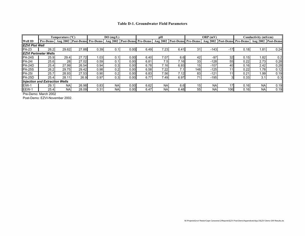
Table D-1. Groundwater Field Parameters

Well ID Temperature (°C) DO (mg/L) pH ORP (mV) Conductivity (mS/cm)

Pre-Demo Aug 2002 Post-Demo Pre-Demo Aug 2002 Post-Demo Pre-Demo Aug 2002 Post-Demo Pre-Demo Aug 2002 Post-Demo Pre-Demo Aug 2002 Post-Demo EZVI Plot Well PA-23 26.2 29.62 27.88 0.39 0.1 0.00 6.49 7.23 6.41 31 -143 -17 0.18 1.81 0.24 EZVI Perimeter Wells PA-24S 25.9 29.4 27.72 1.03 0.1 0.00 6.40 7.07 6.6 42 -97 32 0.15 1.82 0.2 PA-24I 25.6 28 27.02 0.59 0.1 0.00 6.81 7.5 7.16 33 -128 55 0.22 2.73 0.28 PA-24D 25.4 27.99 26.54 0.94 0.3 0.00 6.78 7.16 6.93 15 -107 40 0.16 2.42 0.28 PA-25S 26.2 29.75 29.42 0.98 0.2 0.00 6.58 7.22 7.1 148 -125 11 0.22 1.78 0.12 PA-25I 25.7 28.93 27.53 0.90 0.2 0.00 6.83 7.56 7.12 83 -121 11 0.21 1.99 0.19 PA-25D 25.4 28.11 26.9 0.97 0.3 0.00 6.77 7.49 6.97 71 -195 3 0.33 3.1 0.3 Injection and Extraction Wells EIW-1 29.1 NA 26.98 0.83 NA 0.00 6.62 NA 6.6 15 NA 17 0.16 NA 0.19 EEW-1 25.4 NA 28.09 0.31 NA 0.00 6.47 NA 6.48 55 NA 106 0.16 NA 0.19 Pre-Demo: March 2002 Post-Demo: EZVI-November 2002.

M:\Projects\Envir Restor\Cape Canaveral 2\Reports\EZVI Post-Demo\Appendices\App D\EZVI Demo GW Results.xls

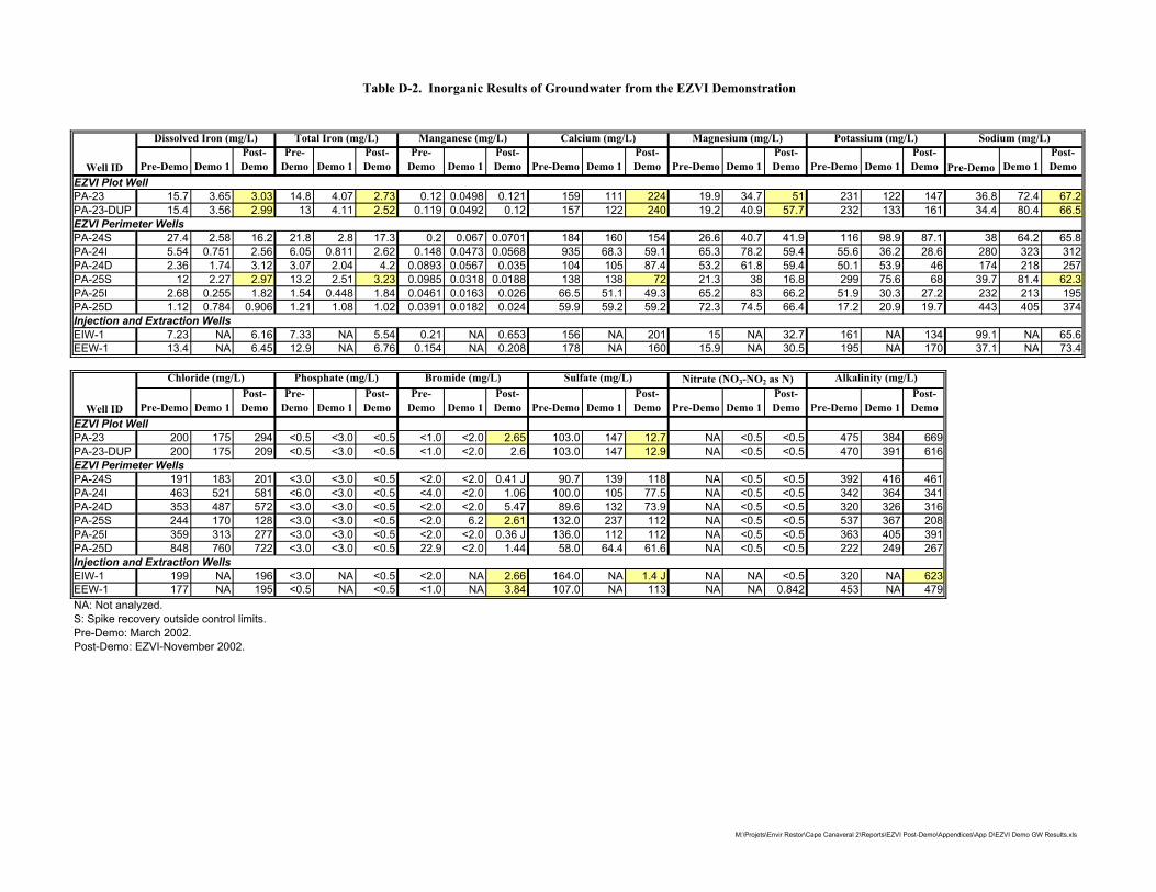
Table D-2. Inorganic Results of Groundwater from the EZVI Demonstration

Well ID

Dissolved Iron (mg/L) Total Iron (mg/L) Manganese (mg/L) Calcium (mg/L) Magnesium (mg/L) Potassium (mg/L) Sodium (mg/L)

Pre-Demo Demo 1 Post-Demo

Pre-Demo Demo 1

Post-Demo

Pre-Demo Demo 1

Post-Demo Pre-Demo Demo 1

Post-Demo Pre-Demo Demo 1

Post-Demo Pre-Demo Demo 1

Post-Demo Pre-Demo Demo 1

Post-Demo

EZVI Plot Well PA-23 15.7 3.65 3.03 14.8 4.07 2.73 0.12 0.0498 0.121 159 111 224 19.9 34.7 51 231 122 147 36.8 72.4 67.2 PA-23-DUP 15.4 3.56 2.99 13 4.11 2.52 0.119 0.0492 0.12 157 122 240 19.2 40.9 57.7 232 133 161 34.4 80.4 66.5 EZVI Perimeter Wells PA-24S 27.4 2.58 16.2 21.8 2.8 17.3 0.2 0.067 0.0701 184 160 154 26.6 40.7 41.9 116 98.9 87.1 38 64.2 65.8 PA-24I 5.54 0.751 2.56 6.05 0.811 2.62 0.148 0.0473 0.0568 935 68.3 59.1 65.3 78.2 59.4 55.6 36.2 28.6 280 323 312 PA-24D 2.36 1.74 3.12 3.07 2.04 4.2 0.0893 0.0567 0.035 104 105 87.4 53.2 61.8 59.4 50.1 53.9 46 174 218 257 PA-25S 12 2.27 2.97 13.2 2.51 3.23 0.0985 0.0318 0.0188 138 138 72 21.3 38 16.8 299 75.6 68 39.7 81.4 62.3 PA-25I 2.68 0.255 1.82 1.54 0.448 1.84 0.0461 0.0163 0.026 66.5 51.1 49.3 65.2 83 66.2 51.9 30.3 27.2 232 213 195 PA-25D 1.12 0.784 0.906 1.21 1.08 1.02 0.0391 0.0182 0.024 59.9 59.2 59.2 72.3 74.5 66.4 17.2 20.9 19.7 443 405 374 Injection and Extraction Wells EIW-1 7.23 NA 6.16 7.33 NA 5.54 0.21 NA 0.653 156 NA 201 15 NA 32.7 161 NA 134 99.1 NA 65.6 EEW-1 13.4 NA 6.45 12.9 NA 6.76 0.154 NA 0.208 178 NA 160 15.9 NA 30.5 195 NA 170 37.1 NA 73.4

Well ID

Chloride (mg/L) Phosphate (mg/L) Bromide (mg/L) Sulfate (mg/L) Nitrate (NO3-NO2 as N) Alkalinity (mg/L)

Pre-Demo Demo 1 Post-Demo

Pre-Demo Demo 1

Post-Demo

Pre-Demo Demo 1

Post-Demo Pre-Demo Demo 1

Post-Demo Pre-Demo Demo 1

Post-Demo Pre-Demo Demo 1

Post-Demo

EZVI Plot Well PA-23 200 175 294 <0.5 <3.0 <0.5 <1.0 <2.0 2.65 103.0 147 12.7 NA <0.5 <0.5 475 384 669 PA-23-DUP 200 175 209 <0.5 <3.0 <0.5 <1.0 <2.0 2.6 103.0 147 12.9 NA <0.5 <0.5 470 391 616 EZVI Perimeter Wells PA-24S 191 183 201 <3.0 <3.0 <0.5 <2.0 <2.0 0.41 J 90.7 139 118 NA <0.5 <0.5 392 416 461 PA-24I 463 521 581 <6.0 <3.0 <0.5 <4.0 <2.0 1.06 100.0 105 77.5 NA <0.5 <0.5 342 364 341 PA-24D 353 487 572 <3.0 <3.0 <0.5 <2.0 <2.0 5.47 89.6 132 73.9 NA <0.5 <0.5 320 326 316 PA-25S 244 170 128 <3.0 <3.0 <0.5 <2.0 6.2 2.61 132.0 237 112 NA <0.5 <0.5 537 367 208 PA-25I 359 313 277 <3.0 <3.0 <0.5 <2.0 <2.0 0.36 J 136.0 112 112 NA <0.5 <0.5 363 405 391 PA-25D 848 760 722 <3.0 <3.0 <0.5 22.9 <2.0 1.44 58.0 64.4 61.6 NA <0.5 <0.5 222 249 267 Injection and Extraction Wells EIW-1 199 NA 196 <3.0 NA <0.5 <2.0 NA 2.66 164.0 NA 1.4 J NA NA <0.5 320 NA 623 EEW-1 177 NA 195 <0.5 NA <0.5 <1.0 NA 3.84 107.0 NA 113 NA NA 0.842 453 NA 479 NA: Not analyzed. S: Spike recovery outside control limits.Pre-Demo: March 2002.Post-Demo: EZVI-November 2002.

M:\Projets\Envir Restor\Cape Canaveral 2\Reports\EZVI Post-Demo\Appendices\App D\EZVI Demo GW Results.xls

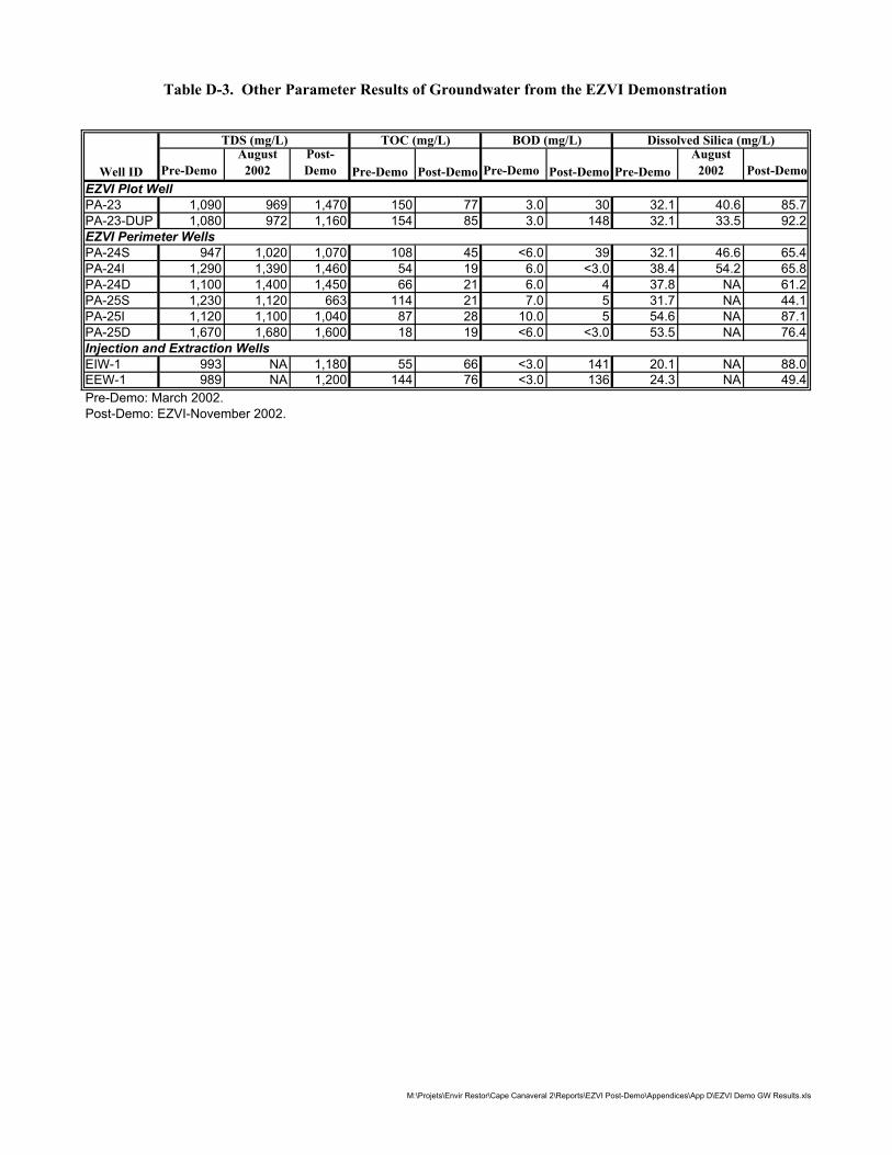
Table D-3. Other Parameter Results of Groundwater from the EZVI Demonstration

Well ID

TDS (mg/L) TOC (mg/L) BOD (mg/L) Dissolved Silica (mg/L)

Pre-Demo August

2002 Post-Demo Pre-Demo Post-Demo Pre-Demo Post-Demo Pre-Demo

August 2002 Post-Demo

EZVI Plot Well PA-23 1,090 969 1,470 150 77 3.0 30 32.1 40.6 85.7 PA-23-DUP 1,080 972 1,160 154 85 3.0 148 32.1 33.5 92.2 EZVI Perimeter Wells PA-24S 947 1,020 1,070 108 45 <6.0 39 32.1 46.6 65.4 PA-24I 1,290 1,390 1,460 54 19 6.0 <3.0 38.4 54.2 65.8 PA-24D 1,100 1,400 1,450 66 21 6.0 4 37.8 NA 61.2 PA-25S 1,230 1,120 663 114 21 7.0 5 31.7 NA 44.1 PA-25I 1,120 1,100 1,040 87 28 10.0 5 54.6 NA 87.1 PA-25D 1,670 1,680 1,600 18 19 <6.0 <3.0 53.5 NA 76.4 Injection and Extraction Wells EIW-1 993 NA 1,180 55 66 <3.0 141 20.1 NA 88.0 EEW-1 989 NA 1,200 144 76 <3.0 136 24.3 NA 49.4 Pre-Demo: March 2002. Post-Demo: EZVI-November 2002.

M:\Projets\Envir Restor\Cape Canaveral 2\Reports\EZVI Post-Demo\Appendices\App D\EZVI Demo GW Results.xls

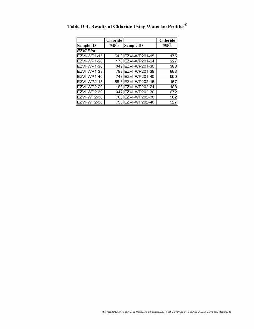
Table D-4. Results of Chloride Using Waterloo Profiler®

Chloride Chloride Sample ID mg/L Sample ID mg/L EZVI Plot EZVI-WP1-15 64.8 EZVI-WP201-15 175 EZVI-WP1-20 170 EZVI-WP201-24 227 EZVI-WP1-30 349 EZVI-WP201-30 388 EZVI-WP1-38 783 EZVI-WP201-38 993 EZVI-WP1-40 743 EZVI-WP201-40 990 EZVI-WP2-15 88.8 EZVI-WP202-15 157 EZVI-WP2-20 188 EZVI-WP202-24 188 EZVI-WP2-30 347 EZVI-WP202-30 672 EZVI-WP2-36 763 EZVI-WP202-38 902 EZVI-WP2-38 798 EZVI-WP202-40 927

M:\Projects\Envir Restor\Cape Canaveral 2\Reports\EZVI Post-Demo\Appendices\App D\EZVI Demo GW Results.xls

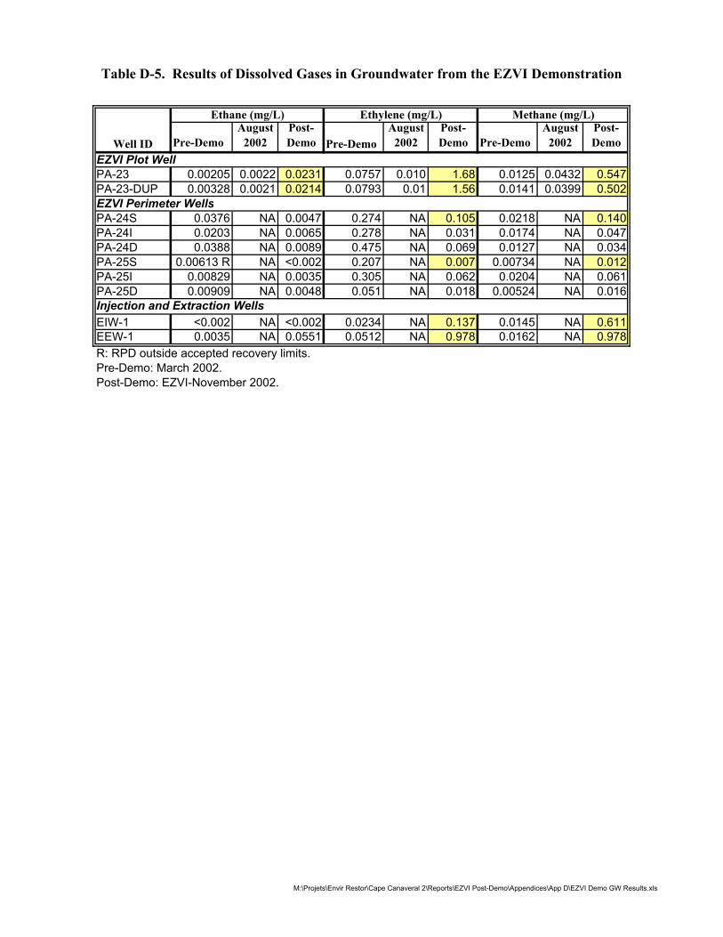
Table D-5. Results of Dissolved Gases in Groundwater from the EZVI Demonstration

Well ID

Ethane (mg/L) Ethylene (mg/L) Methane (mg/L)

Pre-Demo August

2002 Post-Demo Pre-Demo

August 2002

Post-Demo Pre-Demo

August 2002

Post-Demo

EZVI Plot Well PA-23 0.00205 0.0022 0.0231 0.0757 0.010 1.68 0.0125 0.0432 0.547 PA-23-DUP 0.00328 0.0021 0.0214 0.0793 0.01 1.56 0.0141 0.0399 0.502 EZVI Perimeter Wells PA-24S 0.0376 NA 0.0047 0.274 NA 0.105 0.0218 NA 0.140 PA-24I 0.0203 NA 0.0065 0.278 NA 0.031 0.0174 NA 0.047 PA-24D 0.0388 NA 0.0089 0.475 NA 0.069 0.0127 NA 0.034 PA-25S 0.00613 R NA <0.002 0.207 NA 0.007 0.00734 NA 0.012 PA-25I 0.00829 NA 0.0035 0.305 NA 0.062 0.0204 NA 0.061 PA-25D 0.00909 NA 0.0048 0.051 NA 0.018 0.00524 NA 0.016 Injection and Extraction Wells EIW-1 <0.002 NA <0.002 0.0234 NA 0.137 0.0145 NA 0.611 EEW-1 0.0035 NA 0.0551 0.0512 NA 0.978 0.0162 NA 0.978 R: RPD outside accepted recovery limits.Pre-Demo: March 2002.Post-Demo: EZVI-November 2002.

M:\Projets\Envir Restor\Cape Canaveral 2\Reports\EZVI Post-Demo\Appendices\App D\EZVI Demo GW Results.xls

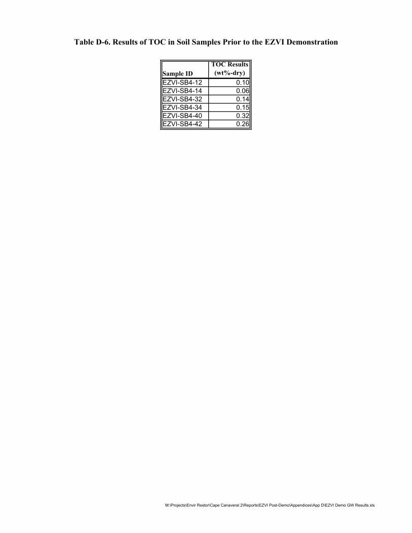
Table D-6. Results of TOC in Soil Samples Prior to the EZVI Demonstration

TOC Results Sample ID (wt%-dry) EZVI-SB4-12 0.10 EZVI-SB4-14 0.06 EZVI-SB4-32 0.14 EZVI-SB4-34 0.15 EZVI-SB4-40 0.32 EZVI-SB4-42 0.26

M:\Projects\Envir Restor\Cape Canaveral 2\Reports\EZVI Post-Demo\Appendices\App D\EZVI Demo GW Results.xls

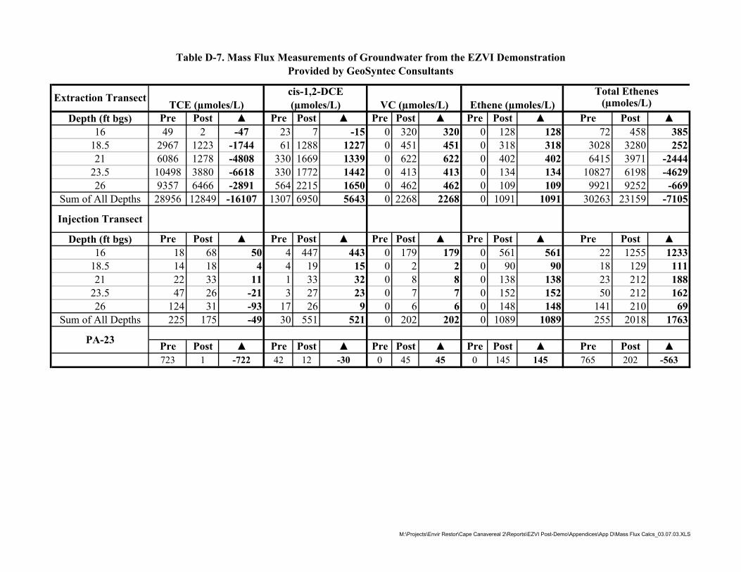
Table D-7. Mass Flux Measurements of Groundwater from the EZVI DemonstrationProvided by GeoSyntec Consultants

Extraction Transect TCE (µmoles/L)

cis-1,2-DCE (µmoles/L) VC (µmoles/L) Ethene (µmoles/L)

Total Ethenes (µmoles/L)

Depth (ft bgs) Pre Post ▲ Pre Post ▲ Pre Post ▲ Pre Post ▲ Pre Post ▲ 16 49 2 -47 23 7 -15 0 320 320 0 128 128 72 458 385

18.5 2967 1223 -1744 61 1288 1227 0 451 451 0 318 318 3028 3280 252 21 6086 1278 -4808 330 1669 1339 0 622 622 0 402 402 6415 3971 -2444

23.5 10498 3880 -6618 330 1772 1442 0 413 413 0 134 134 10827 6198 -4629 26 9357 6466 -2891 564 2215 1650 0 462 462 0 109 109 9921 9252 -669

Sum of All Depths 28956 12849 -16107 1307 6950 5643 0 2268 2268 0 1091 1091 30263 23159 -7105

Injection Transect

Depth (ft bgs) Pre Post ▲ Pre Post ▲ Pre Post ▲ Pre Post ▲ Pre Post ▲ 16 18 68 50 4 447 443 0 179 179 0 561 561 22 1255 1233

18.5 14 18 4 4 19 15 0 2 2 0 90 90 18 129 111 21 22 33 11 1 33 32 0 8 8 0 138 138 23 212 188

23.5 47 26 -21 3 27 23 0 7 7 0 152 152 50 212 162 26 124 31 -93 17 26 9 0 6 6 0 148 148 141 210 69

Sum of All Depths 225 175 -49 30 551 521 0 202 202 0 1089 1089 255 2018 1763

PA-23 Pre Post ▲ Pre Post ▲ Pre Post ▲ Pre Post ▲ Pre Post ▲ 723 1 -722 42 12 -30 0 45 45 0 145 145 765 202 -563

M:\Projects\Envir Restor\Cape Canavereal 2\Reports\EZVI Post-Demo\Appendices\App D\Mass Flux Calcs_03.07.03.XLS

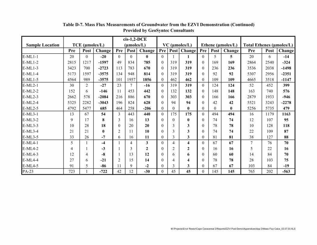
Table D-7. Mass Flux Measurements of Groundwater from the EZVI Demonstration (Continued)Provided by GeoSyntec Consultants

Sample Location TCE (µmoles/L) cis-1,2-DCE (µmoles/L) VC (µmoles/L) Ethene (µmoles/L) Total Ethenes (µmoles/L)

Pre Post Change Pre Post Change Pre Post Change Pre Post Change Pre Post Change E-ML1-1 20 0 -20 0 0 0 0 1 1 0 5 5 20 6 -14 E-ML1-2 2815 1217 -1597 49 834 785 0 319 319 0 169 169 2864 2540 -324 E-ML1-3 3423 700 -2723 113 783 670 0 319 319 0 236 236 3536 2038 -1498 E-ML1-4 5173 1597 -3575 134 948 814 0 319 319 0 92 92 5307 2956 -2351 E-ML1-5 4564 989 -3575 101 1957 1856 0 462 462 0 109 109 4665 3518 -1147 E-ML2-1 30 2 -27 23 7 -16 0 319 319 0 124 124 52 452 399 E-ML2-2 152 6 -146 11 453 442 0 132 132 0 148 148 163 740 576 E-ML2-3 2662 578 -2084 216 886 670 0 303 303 0 166 166 2879 1933 -946 E-ML2-4 5325 2282 -3043 196 824 628 0 94 94 0 42 42 5521 3243 -2278 E-ML2-5 4792 5477 685 464 258 -206 0 0 0 0 0 0 5256 5735 479 E-ML3-1 13 67 54 3 443 440 0 175 175 0 494 494 16 1179 1163 E-ML3-2 9 17 8 3 16 13 0 0 0 0 74 74 12 107 95 E-ML3-3 10 28 18 0 20 20 0 3 3 0 78 78 10 128 118 E-ML3-4 21 21 0 2 11 10 0 3 3 0 74 74 22 109 87 E-ML3-5 33 26 -7 6 16 11 0 3 3 0 81 81 38 127 88 E-ML4-1 5 1 -4 1 4 3 0 4 4 0 67 67 7 76 70 E-ML4-2 4 1 -3 1 3 2 0 2 2 0 16 16 5 22 16 E-ML4-3 12 4 -8 1 13 12 0 6 6 0 60 60 14 84 70 E-ML4-4 27 6 -21 2 15 14 0 4 4 0 78 78 28 103 75 E-ML4-5 91 5 -86 11 9 -2 0 3 3 0 67 67 103 84 -19 PA-23 723 1 -722 42 12 -30 0 45 45 0 145 145 765 202 -563

M:\Projects\Envir Restor\Cape Canavereal 2\Reports\EZVI Post-Demo\Appendices\App D\Mass Flux Calcs_03.07.03.XLS

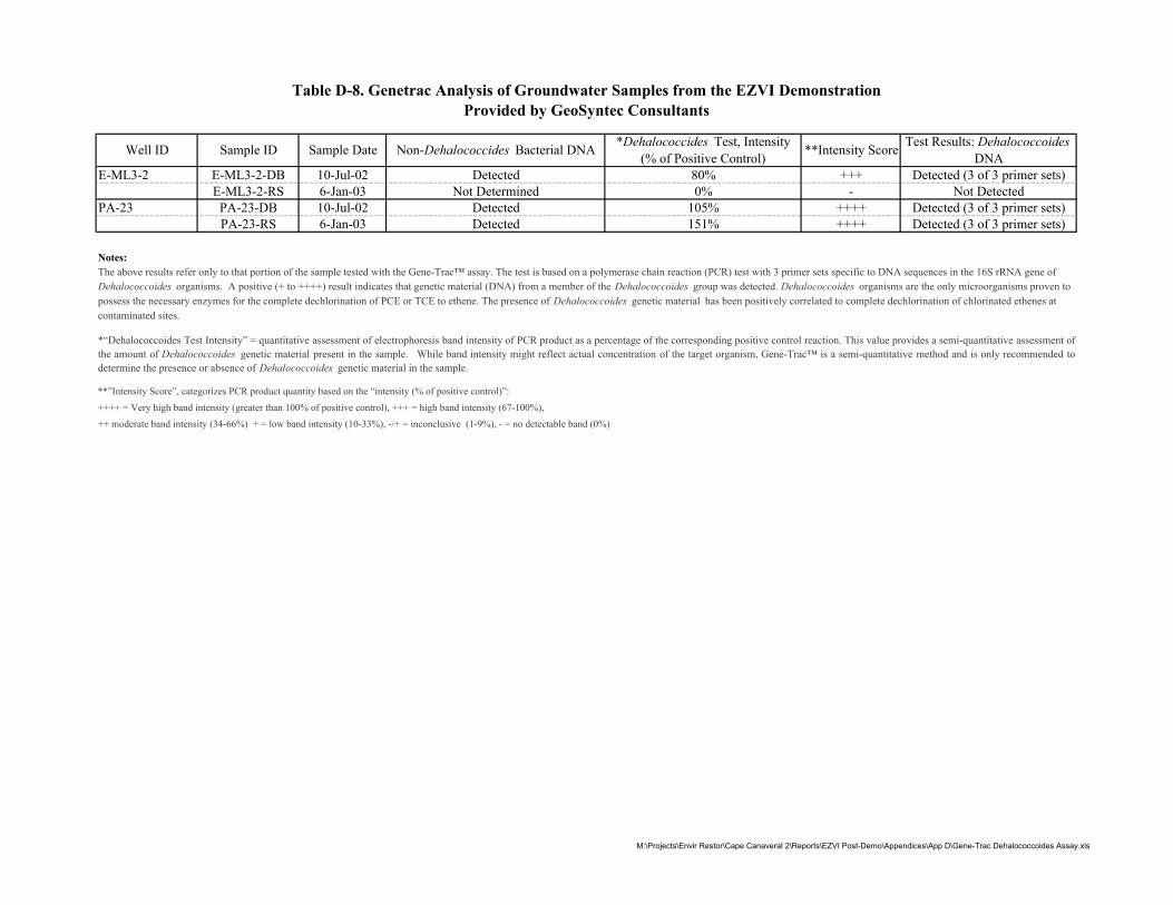
Table D-8. Genetrac Analysis of Groundwater Samples from the EZVI DemonstrationProvided by GeoSyntec Consultants

Well ID Sample ID Sample Date Non-Dehalococcides Bacterial DNA *Dehalococcides Test, Intensity (% of Positive Control) **Intensity Score Test Results: Dehalococcoides

DNA E-ML3-2 E-ML3-2-DB

E-ML3-2-RS 10-Jul-02 6-Jan-03

Detected Not Determined

80% 0%

+++ -

Detected (3 of 3 primer sets) Not Detected

PA-23 PA-23-DB PA-23-RS

10-Jul-02 6-Jan-03

Detected Detected

105% 151%

++++ ++++

Detected (3 of 3 primer sets) Detected (3 of 3 primer sets)

Notes: The above results refer only to that portion of the sample tested with the Gene-Trac™ assay. The test is based on a polymerase chain reaction (PCR) test with 3 primer sets specific to DNA sequences in the 16S rRNA gene of Dehalococcoides organisms. A positive (+ to ++++) result indicates that genetic material (DNA) from a member of the Dehalococcoides group was detected. Dehalococcoides organisms are the only microorganisms proven to possess the necessary enzymes for the complete dechlorination of PCE or TCE to ethene. The presence of Dehalococcoides genetic material has been positively correlated to complete dechlorination of chlorinated ethenes at contaminated sites.

*“Dehalococcoides Test Intensity” = quantitative assessment of electrophoresis band intensity of PCR product as a percentage of the corresponding positive control reaction. This value provides a semi-quantitative assessment of the amount of Dehalococcoides genetic material present in the sample. While band intensity might reflect actual concentration of the target organism, Gene-Trac™ is a semi-quantitative method and is only recommended to determine the presence or absence of Dehalococcoides genetic material in the sample.

**”Intensity Score”, categorizes PCR product quantity based on the “intensity (% of positive control)”:

++++ = Very high band intensity (greater than 100% of positive control), +++ = high band intensity (67-100%),

++ moderate band intensity (34-66%) + = low band intensity (10-33%), -/+ = inconclusive (1-9%), - = no detectable band (0%)

M:\Projects\Envir Restor\Cape Canaveral 2\Reports\EZVI Post-Demo\Appendices\App D\Gene-Trac Dehalococcoides Assay.xls

Appendix E

Quality Assurance/Quality Control Information

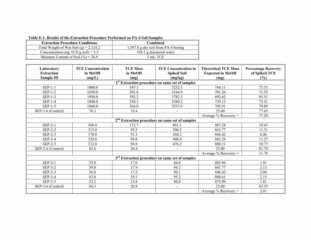
Table E-1. Results of the Extraction Procedure Performed on PA-4 Soil Samples Extraction Procedure Conditions Combined

Total Weight of Wet Soil (g) = 2,124.2 1,587.8 g dry soil from PA-4 boring Concentration (mg TCE/g soil) = 3.3 529.3 g deionized water Moisture Content of Soil (%) = 24.9 5 mL TCE

Laboratory Extraction Sample ID

TCE Concentration in MeOH

(mg/L)

TCE Mass in MeOH

(mg)

TCE Concentration in Spiked Soil

(mg/kg)

Theoretical TCE Mass Expected in MeOH

(mg)

Percentage Recovery of Spiked TCE

(%) 1st Extraction procedure on same set of samples

SEP-1-1 1800.0 547.1 3252.5 744.11 73.53 SEP-1-2 1650.0 501.8 3164.9 701.26 71.55 SEP-1-3 1950.0 592.2 3782.3 692.62 85.51 SEP-1-4 1840.0 558.1 3340.2 739.13 75.51 SEP-1-5 1860.0 564.0 3533.9 705.91 79.89

SEP-1-6 (Control) 78.3 19.4 - 25.00 77.65 Average % Recovery = 77.20

2nd Extraction procedure on same set of samples SEP-2-1 568.0 172.7 861.1 887.28 19.47 SEP-2-2 315.0 95.5 500.5 843.77 11.31 SEP-2-3 170.0 51.3 268.2 846.42 6.06 SEP-2-4 329.0 99.8 498.4 885.29 11.27 SEP-2-5 312.0 94.8 476.3 880.31 10.77

SEP-2-6 (Control) 82.6 20.4 - 25.00 81.79 Average % Recovery = 11.78

3rd Extraction procedure on same set of samples SEP-3-1 55.8 17.0 84.6 885.96 1.91 SEP-3-2 59.0 17.9 94.2 841.77 2.13 SEP-3-3 56.8 17.2 90.1 846.42 2.04 SEP-3-4 63.0 19.1 95.2 888.61 2.15 SEP-3-5 52.2 15.8 80.0 875.99 1.81

SEP-3-6 (Control) 84.3 20.9 - 25.00 83.55 Average % Recovery = 2.01

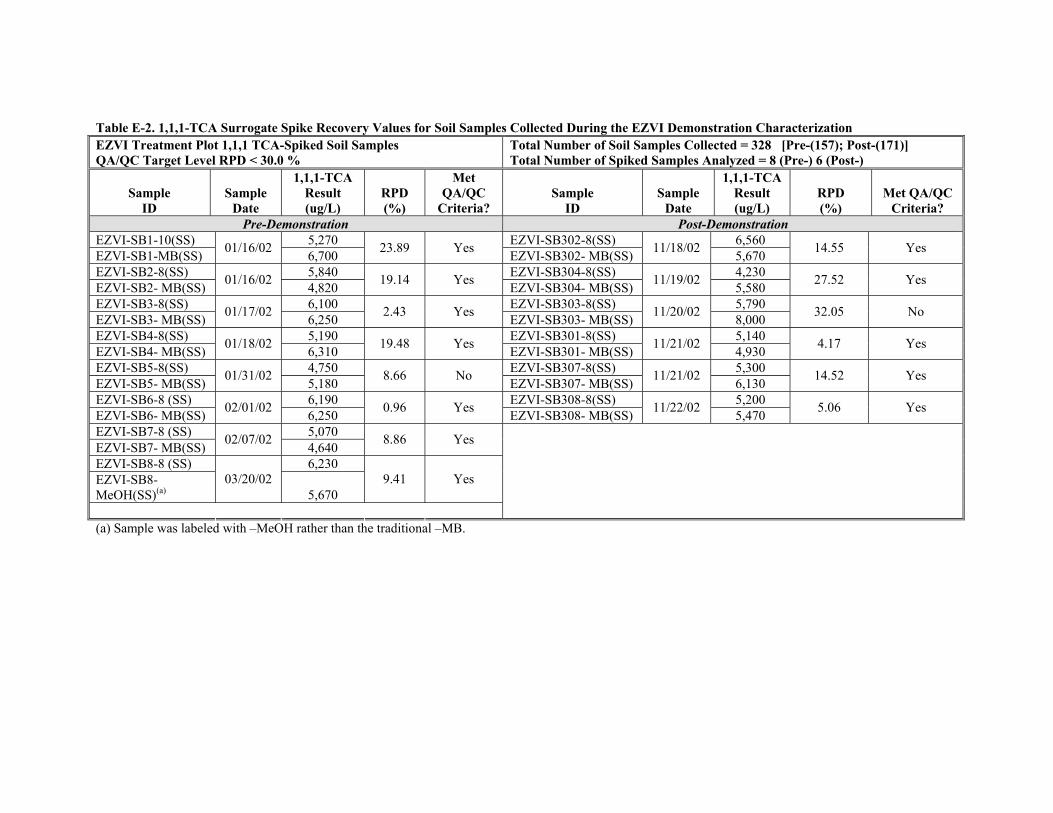
Table E-2. 1,1,1-TCA Surrogate Spike Recovery Values for Soil Samples Collected During the EZVI Demonstration Characterization EZVI Treatment Plot 1,1,1 TCA-Spiked Soil Samples Total Number of Soil Samples Collected = 328 [Pre-(157); Post-(171)] QA/QC Target Level RPD < 30.0 % Total Number of Spiked Samples Analyzed = 8 (Pre-) 6 (Post-)

1,1,1-TCA Met 1,1,1-TCA Sample Sample Result RPD QA/QC Sample Sample Result RPD Met QA/QC

ID Date (ug/L) (%) Criteria? ID Date (ug/L) (%) Criteria? Pre-Demonstration Post-Demonstration

EZVI-SB1-10(SS) 5,270 EZVI-SB302-8(SS) 6,560 01/16/02 23.89 Yes 11/18/02 14.55 Yes EZVI-SB1-MB(SS) 6,700 EZVI-SB302- MB(SS) 5,670 EZVI-SB2-8(SS) 5,840 EZVI-SB304-8(SS) 4,230 01/16/02 19.14 Yes 11/19/02 27.52 Yes EZVI-SB2- MB(SS) 4,820 EZVI-SB304- MB(SS) 5,580 EZVI-SB3-8(SS) 6,100 EZVI-SB303-8(SS) 5,790 01/17/02 2.43 Yes 11/20/02 32.05 No EZVI-SB3- MB(SS) 6,250 EZVI-SB303- MB(SS) 8,000 EZVI-SB4-8(SS) 5,190 EZVI-SB301-8(SS) 5,140 01/18/02 19.48 Yes 11/21/02 4.17 Yes EZVI-SB4- MB(SS) 6,310 EZVI-SB301- MB(SS) 4,930 EZVI-SB5-8(SS) 4,750 EZVI-SB307-8(SS) 5,300 01/31/02 8.66 No 11/21/02 14.52 Yes EZVI-SB5- MB(SS) 5,180 EZVI-SB307- MB(SS) 6,130 EZVI-SB6-8 (SS) 6,190 EZVI-SB308-8(SS) 5,200 02/01/02 0.96 Yes 11/22/02 5.06 Yes EZVI-SB6- MB(SS) 6,250 EZVI-SB308- MB(SS) 5,470 EZVI-SB7-8 (SS) 5,070 02/07/02 8.86 Yes EZVI-SB7- MB(SS) 4,640 EZVI-SB8-8 (SS) 6,230 EZVI-SB8- 03/20/02 9.41 Yes MeOH(SS)(a) 5,670

(a) Sample was labeled with –MeOH rather than the traditional –MB.

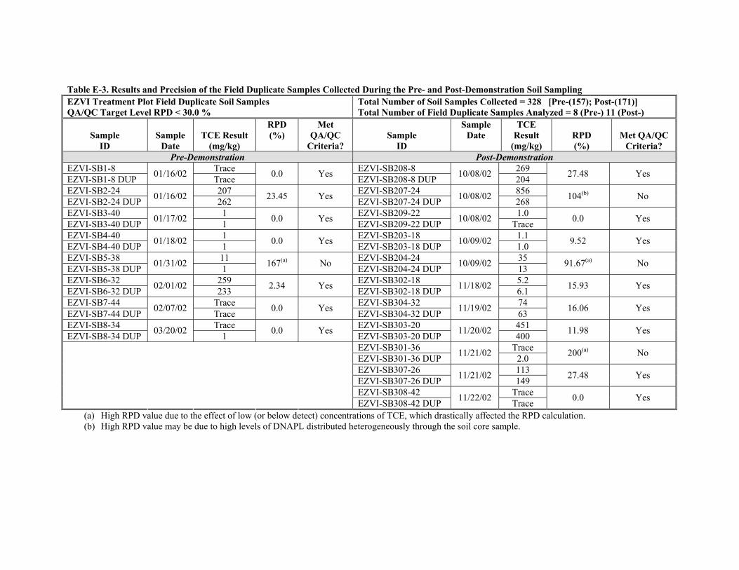
Table E-3. Results and Precision of the Field Duplicate Samples Collected During the Pre- and Post-Demonstration Soil Sampling EZVI Treatment Plot Field Duplicate Soil Samples Total Number of Soil Samples Collected = 328 [Pre-(157); Post-(171)] QA/QC Target Level RPD < 30.0 % Total Number of Field Duplicate Samples Analyzed = 8 (Pre-) 11 (Post-)

RPD Met Sample TCE Sample Sample TCE Result (%) QA/QC Sample Date Result RPD Met QA/QC

ID Date (mg/kg) Criteria? ID (mg/kg) (%) Criteria? Pre-Demonstration Post-Demonstration

EZVI-SB1-8 Trace EZVI-SB208-8 269 01/16/02 0.0 Yes 10/08/02 27.48 Yes EZVI-SB1-8 DUP Trace EZVI-SB208-8 DUP 204 EZVI-SB2-24 207 EZVI-SB207-24 856 104(b)01/16/02 23.45 Yes 10/08/02 No EZVI-SB2-24 DUP 262 EZVI-SB207-24 DUP 268 EZVI-SB3-40 1 EZVI-SB209-22 1.0 01/17/02 0.0 Yes 10/08/02 0.0 Yes EZVI-SB3-40 DUP 1 EZVI-SB209-22 DUP Trace EZVI-SB4-40 1 EZVI-SB203-18 1.1 01/18/02 0.0 Yes 10/09/02 9.52 Yes EZVI-SB4-40 DUP 1 EZVI-SB203-18 DUP 1.0 EZVI-SB5-38 11 167(a) EZVI-SB204-24 35 91.67(a)01/31/02 No 10/09/02 No EZVI-SB5-38 DUP 1 EZVI-SB204-24 DUP 13 EZVI-SB6-32 259 EZVI-SB302-18 5.2 02/01/02 2.34 Yes 11/18/02 15.93 Yes EZVI-SB6-32 DUP 233 EZVI-SB302-18 DUP 6.1 EZVI-SB7-44 Trace EZVI-SB304-32 74 02/07/02 0.0 Yes 11/19/02 16.06 Yes EZVI-SB7-44 DUP Trace EZVI-SB304-32 DUP 63 EZVI-SB8-34 Trace EZVI-SB303-20 451 03/20/02 0.0 Yes 11/20/02 11.98 Yes EZVI-SB8-34 DUP 1 EZVI-SB303-20 DUP 400

EZVI-SB301-36 Trace 200(a)11/21/02 No EZVI-SB301-36 DUP 2.0 EZVI-SB307-26 113 11/21/02 27.48 Yes EZVI-SB307-26 DUP 149 EZVI-SB308-42 Trace 11/22/02 0.0 Yes EZVI-SB308-42 DUP Trace

(a) High RPD value due to the effect of low (or below detect) concentrations of TCE, which drastically affected the RPD calculation. (b) High RPD value may be due to high levels of DNAPL distributed heterogeneously through the soil core sample.

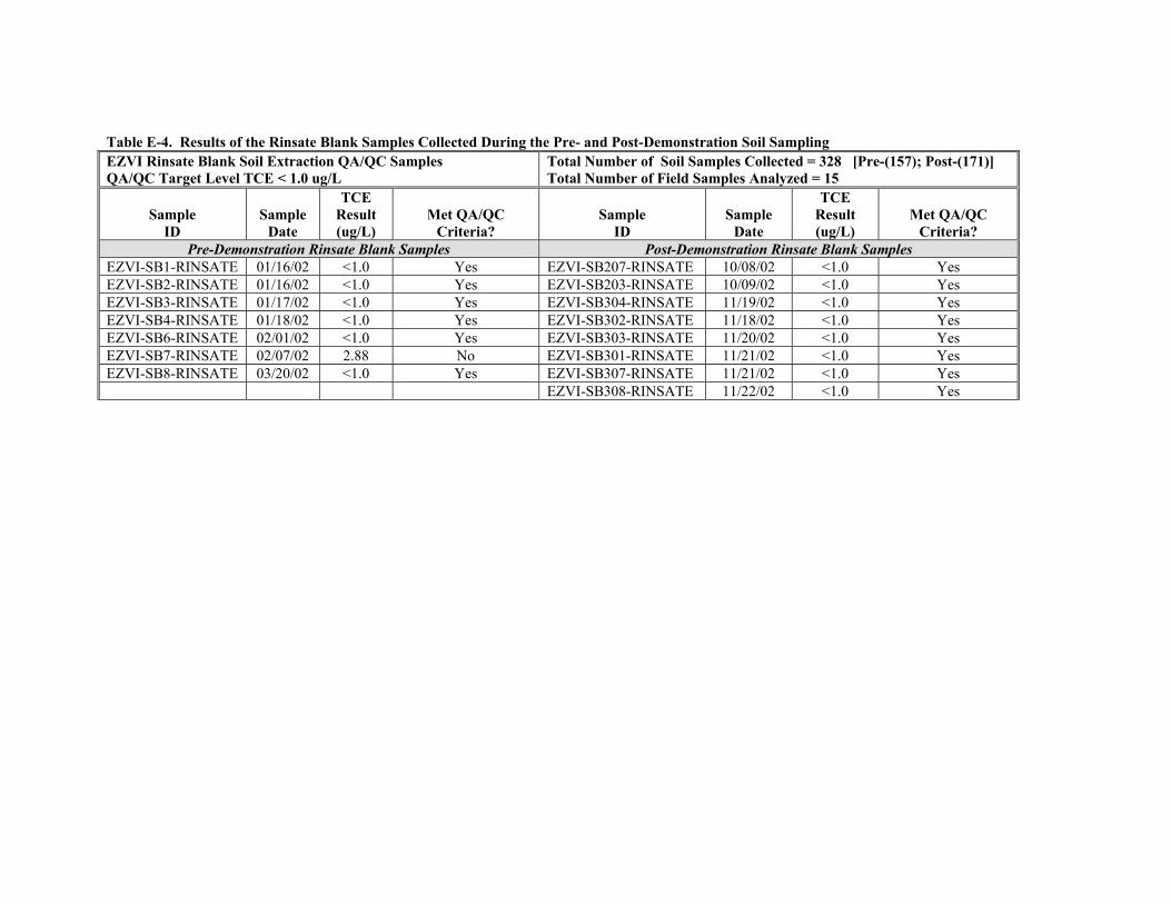
Table E-4. Results of the Rinsate Blank Samples Collected During the Pre- and Post-Demonstration Soil Sampling EZVI Rinsate Blank Soil Extraction QA/QC Samples QA/QC Target Level TCE < 1.0 ug/L

Total Number of Soil Samples Collected = 328 [Pre-(157); Post-(171)] Total Number of Field Samples Analyzed = 15

Sample ID

Sample Date

TCE Result (ug/L)

Met QA/QC Criteria?

Sample ID

Sample Date

TCE Result (ug/L)

Met QA/QC Criteria?

Pre-Demonstration Rinsate Blank Samples Post-Demonstration Rinsate Blank Samples EZVI-SB1-RINSATE 01/16/02 <1.0 Yes EZVI-SB207-RINSATE 10/08/02 <1.0 Yes EZVI-SB2-RINSATE 01/16/02 <1.0 Yes EZVI-SB203-RINSATE 10/09/02 <1.0 Yes EZVI-SB3-RINSATE 01/17/02 <1.0 Yes EZVI-SB304-RINSATE 11/19/02 <1.0 Yes EZVI-SB4-RINSATE 01/18/02 <1.0 Yes EZVI-SB302-RINSATE 11/18/02 <1.0 Yes EZVI-SB6-RINSATE 02/01/02 <1.0 Yes EZVI-SB303-RINSATE 11/20/02 <1.0 Yes EZVI-SB7-RINSATE 02/07/02 2.88 No EZVI-SB301-RINSATE 11/21/02 <1.0 Yes EZVI-SB8-RINSATE 03/20/02 <1.0 Yes EZVI-SB307-RINSATE 11/21/02 <1.0 Yes

EZVI-SB308-RINSATE 11/22/02 <1.0 Yes

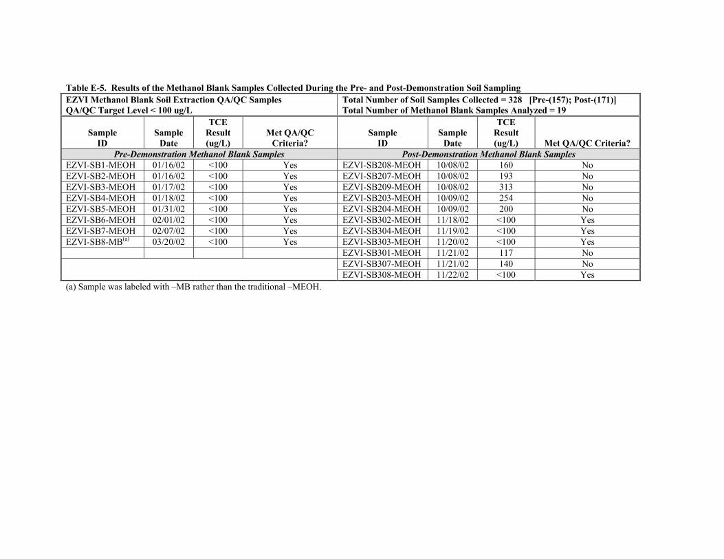
Table E-5. Results of the Methanol Blank Samples Collected During the Pre- and Post-Demonstration Soil Sampling EZVI Methanol Blank Soil Extraction QA/QC Samples QA/QC Target Level < 100 ug/L

Total Number of Soil Samples Collected = 328 [Pre-(157); Post-(171)] Total Number of Methanol Blank Samples Analyzed = 19

Sample ID

Sample Date

TCE Result (ug/L)

Met QA/QC Criteria?

Sample ID

Sample Date

TCE Result (ug/L) Met QA/QC Criteria?

Pre-Demonstration Methanol Blank Samples Post-Demonstration Methanol Blank Samples EZVI-SB1-MEOH 01/16/02 <100 Yes EZVI-SB208-MEOH 10/08/02 160 No EZVI-SB2-MEOH 01/16/02 <100 Yes EZVI-SB207-MEOH 10/08/02 193 No EZVI-SB3-MEOH 01/17/02 <100 Yes EZVI-SB209-MEOH 10/08/02 313 No EZVI-SB4-MEOH 01/18/02 <100 Yes EZVI-SB203-MEOH 10/09/02 254 No EZVI-SB5-MEOH 01/31/02 <100 Yes EZVI-SB204-MEOH 10/09/02 200 No EZVI-SB6-MEOH 02/01/02 <100 Yes EZVI-SB302-MEOH 11/18/02 <100 Yes EZVI-SB7-MEOH 02/07/02 <100 Yes EZVI-SB304-MEOH 11/19/02 <100 Yes EZVI-SB8-MB(a) 03/20/02 <100 Yes EZVI-SB303-MEOH 11/20/02 <100 Yes

EZVI-SB301-MEOH 11/21/02 117 No EZVI-SB307-MEOH 11/21/02 140 No EZVI-SB308-MEOH 11/22/02 <100 Yes

(a) Sample was labeled with –MB rather than the traditional –MEOH.

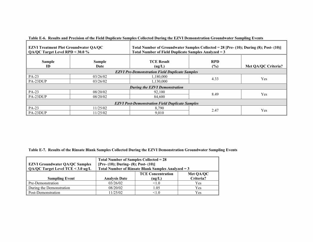
Table E-6. Results and Precision of the Field Duplicate Samples Collected During the EZVI Demonstration Groundwater Sampling Events

EZVI Treatment Plot Groundwater QA/QC QA/QC Target Level RPD < 30.0 %

Total Number of Groundwater Samples Collected = 28 [Pre- (10); During (8); Post- (10)] Total Number of Field Duplicate Samples Analyzed = 3

Sample ID

Sample Date

TCE Result (ug/L)

RPD (%) Met QA/QC Criteria?

EZVI Pre-Demonstration Field Duplicate Samples PA-23 03/26/02 1,180,000 4.33 YesPA-23DUP 03/26/02 1,130,000

During the EZVI Demonstration PA-23 08/20/02 92,100 8.49 YesPA-23DUP 08/20/02 84,600

EZVI Post-Demonstration Field Duplicate Samples PA-23 11/25/02 8,790 2.47 YesPA-23DUP 11/25/02 9,010

Table E-7. Results of the Rinsate Blank Samples Collected During the EZVI Demonstration Groundwater Sampling Events

EZVI Groundwater QA/QC Samples QA/QC Target Level TCE < 3.0 ug/L

Total Number of Samples Collected = 28 [Pre- (10); During- (8); Post- (10)] Total Number of Rinsate Blank Samples Analyzed = 3

Sampling Event Analysis Date TCE Concentration

(ug/L) Met QA/QC

Criteria? Pre-Demonstration 03/26/02 <1.0 Yes During the Demonstration 08/20/02 1.05 Yes Post-Demonstration 11/25/02 <1.0 Yes

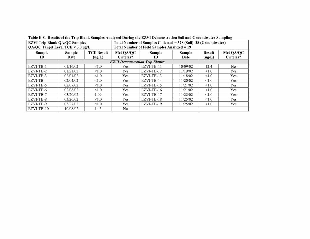
Table E-8. Results of the Trip Blank Samples Analyzed During the EZVI Demonstration Soil and Groundwater Sampling EZVI Trip Blank QA/QC Samples QA/QC Target Level TCE < 3.0 ug/L

Total Number of Samples Collected = 328 (Soil) 28 (Groundwater) Total Number of Field Samples Analyzed = 19

Sample ID

Sample Date

TCE Result (ug/L)

Met QA/QC Criteria?

Sample ID

Sample Date

Result (ug/L)

Met QA/QC Criteria?

EZVI Demonstration Trip Blanks EZVI-TB-1 01/16/02 <1.0 Yes EZVI-TB-11 10/09/02 12.4 No EZVI-TB-2 01/21/02 <1.0 Yes EZVI-TB-12 11/19/02 <1.0 Yes EZVI-TB-3 02/01/02 <1.0 Yes EZVI-TB-13 11/18/02 <1.0 Yes EZVI-TB-4 02/04/02 <1.0 Yes EZVI-TB-14 11/20/02 <1.0 Yes EZVI-TB-5 02/07/02 <1.0 Yes EZVI-TB-15 11/21/02 <1.0 Yes EZVI-TB-6 02/08/02 <1.0 Yes EZVI-TB-16 11/21/02 <1.0 Yes EZVI-TB-7 03/20/02 1.09 Yes EZVI-TB-17 11/22/02 <1.0 Yes EZVI-TB-8 03/26/02 <1.0 Yes EZVI-TB-18 11/25/02 <1.0 Yes EZVI-TB-9 03/27/02 <1.0 Yes EZVI-TB-19 11/25/02 <1.0 Yes EZVI-TB-10 10/08/02 14.5 No

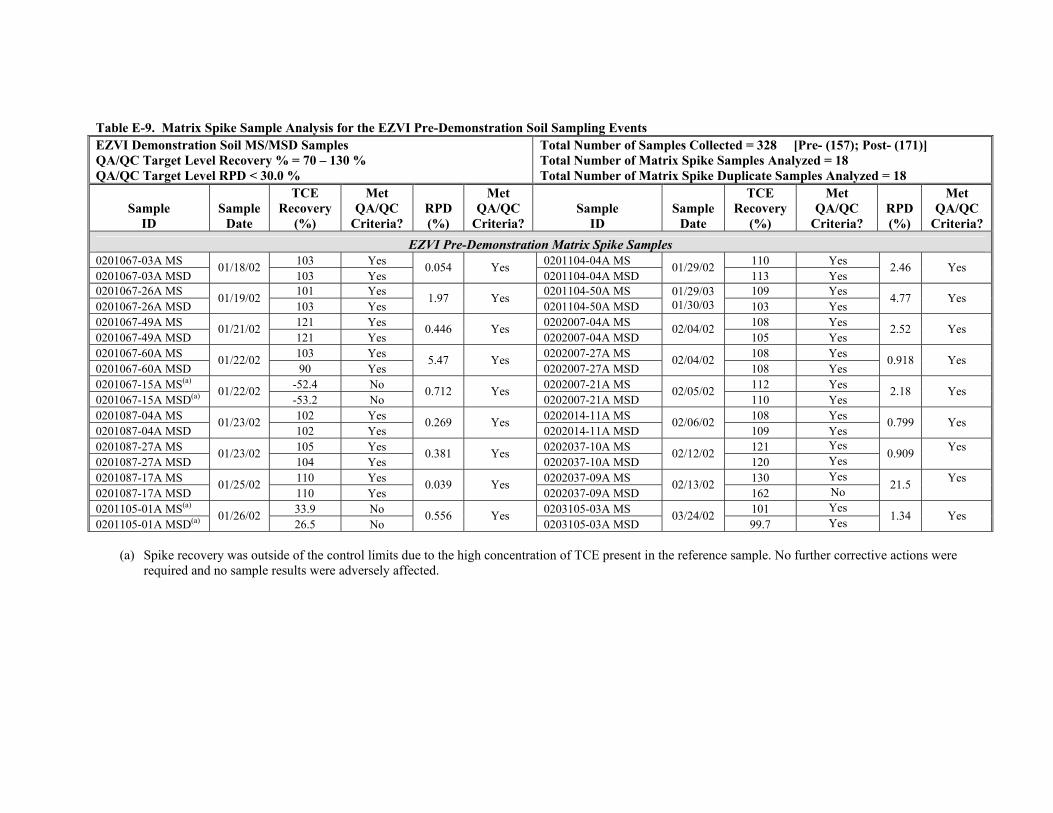
Table E-9. Matrix Spike Sample Analysis for the EZVI Pre-Demonstration Soil Sampling Events EZVI Demonstration Soil MS/MSD Samples QA/QC Target Level Recovery % = 70 – 130 % QA/QC Target Level RPD < 30.0 %

Total Number of Samples Collected = 328 [Pre- (157); Post- (171)] Total Number of Matrix Spike Samples Analyzed = 18 Total Number of Matrix Spike Duplicate Samples Analyzed = 18

Sample ID

Sample Date

TCE Recovery

(%)

Met QA/QC

Criteria? RPD (%)

Met QA/QC

Criteria? Sample

ID Sample

Date

TCE Recovery

(%)

Met QA/QC

Criteria? RPD (%)

Met QA/QC

Criteria? EZVI Pre-Demonstration Matrix Spike Samples

0201067-03A MS 01/18/02 103 Yes 0.054 Yes 0201104-04A MS 01/29/02 110 Yes 2.46 Yes0201067-03A MSD 103 Yes 0201104-04A MSD 113 Yes 0201067-26A MS 01/19/02 101 Yes 1.97 Yes 0201104-50A MS 01/29/03

01/30/03 109 Yes 4.77 Yes

0201067-26A MSD 103 Yes 0201104-50A MSD 103 Yes 0201067-49A MS 01/21/02 121 Yes 0.446 Yes 0202007-04A MS 02/04/02 108 Yes 2.52 Yes0201067-49A MSD 121 Yes 0202007-04A MSD 105 Yes 0201067-60A MS 01/22/02 103 Yes 5.47 Yes 0202007-27A MS 02/04/02 108 Yes 0.918 Yes0201067-60A MSD 90 Yes 0202007-27A MSD 108 Yes 0201067-15A MS(a)

0201067-15A MSD(a) 01/22/02 -52.4 No 0.712 Yes 0202007-21A MS 02/05/02 112 Yes 2.18 Yes-53.2 No 0202007-21A MSD 110 Yes

0201087-04A MS 01/23/02 102 Yes 0.269 Yes 0202014-11A MS 02/06/02 108 Yes 0.799 Yes0201087-04A MSD 102 Yes 0202014-11A MSD 109 Yes 0201087-27A MS 01/23/02 105 Yes 0.381 Yes 0202037-10A MS 02/12/02 121 Yes

0.909 Yes 0201087-27A MSD 104 Yes 0202037-10A MSD 120 Yes 0201087-17A MS 01/25/02 110 Yes 0.039 Yes 0202037-09A MS 02/13/02 130 Yes

21.5 Yes 0201087-17A MSD 110 Yes 0202037-09A MSD 162 No 0201105-01A MS(a)

0201105-01A MSD(a) 01/26/02 33.9 No 0.556 Yes 0203105-03A MS 03/24/02 101 Yes 1.34 Yes

26.5 No 0203105-03A MSD 99.7 Yes

(a) Spike recovery was outside of the control limits due to the high concentration of TCE present in the reference sample. No further corrective actions were required and no sample results were adversely affected.

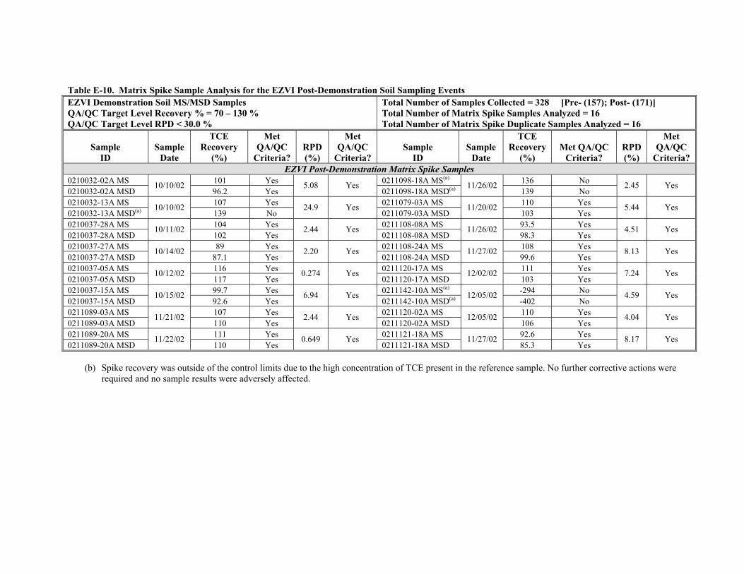
Table E-10. Matrix Spike Sample Analysis for the EZVI Post-Demonstration Soil Sampling Events EZVI Demonstration Soil MS/MSD Samples QA/QC Target Level Recovery % = 70 – 130 % QA/QC Target Level RPD < 30.0 %

Total Number of Samples Collected = 328 [Pre- (157); Post- (171)] Total Number of Matrix Spike Samples Analyzed = 16 Total Number of Matrix Spike Duplicate Samples Analyzed = 16

Sample ID

Sample Date

TCE Recovery

(%)

Met QA/QC

Criteria? RPD (%)

Met QA/QC

Criteria? Sample

ID Sample

Date

TCE Recovery

(%) Met QA/QC

Criteria? RPD (%)

Met QA/QC

Criteria? EZVI Post-Demonstration Matrix Spike Samples

0210032-02A MS 10/10/02 101 Yes 5.08 Yes 0211098-18A MS(a) 11/26/02 136 No 2.45 Yes

0210032-02A MSD 96.2 Yes 0211098-18A MSD(a) 139 No 0210032-13A MS 0210032-13A MSD(a) 10/10/02 107 Yes 24.9 Yes 0211079-03A MS 11/20/02 110 Yes 5.44 Yes

139 No 0211079-03A MSD 103 Yes 0210037-28A MS 10/11/02 104 Yes 2.44 Yes 0211108-08A MS 11/26/02 93.5 Yes 4.51 Yes0210037-28A MSD 102 Yes 0211108-08A MSD 98.3 Yes 0210037-27A MS 10/14/02 89 Yes 2.20 Yes 0211108-24A MS 11/27/02 108 Yes 8.13 Yes0210037-27A MSD 87.1 Yes 0211108-24A MSD 99.6 Yes 0210037-05A MS 10/12/02 116 Yes 0.274 Yes 0211120-17A MS 12/02/02 111 Yes 7.24 Yes0210037-05A MSD 117 Yes 0211120-17A MSD 103 Yes 0210037-15A MS 10/15/02 99.7 Yes 6.94 Yes 0211142-10A MS(a)

12/05/02 -294 No 4.59 Yes0210037-15A MSD 92.6 Yes 0211142-10A MSD(a) -402 No 0211089-03A MS 11/21/02 107 Yes 2.44 Yes 0211120-02A MS 12/05/02 110 Yes 4.04 Yes0211089-03A MSD 110 Yes 0211120-02A MSD 106 Yes 0211089-20A MS 11/22/02 111 Yes 0.649 Yes 0211121-18A MS 11/27/02 92.6 Yes 8.17 Yes0211089-20A MSD 110 Yes 0211121-18A MSD 85.3 Yes

(b) Spike recovery was outside of the control limits due to the high concentration of TCE present in the reference sample. No further corrective actions were required and no sample results were adversely affected.

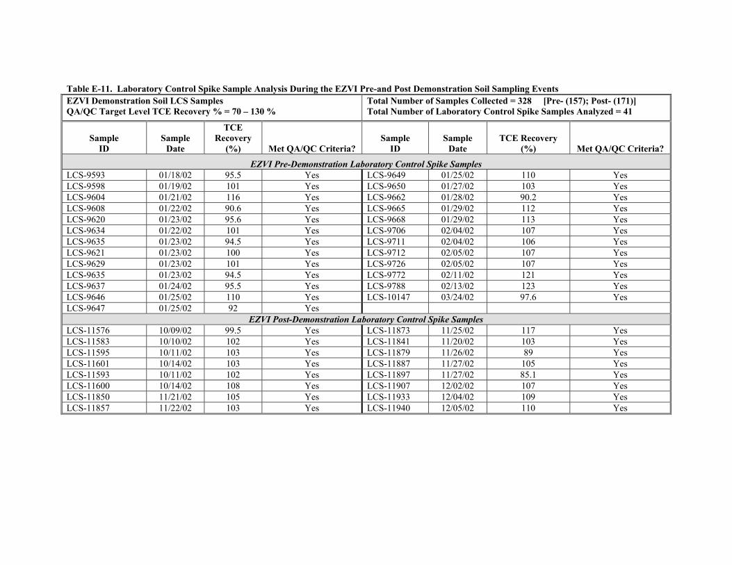
Table E-11. Laboratory Control Spike Sample Analysis During the EZVI Pre-and Post Demonstration Soil Sampling Events EZVI Demonstration Soil LCS Samples QA/QC Target Level TCE Recovery % = 70 – 130 %

Total Number of Samples Collected = 328 [Pre- (157); Post- (171)] Total Number of Laboratory Control Spike Samples Analyzed = 41

Sample ID

Sample Date

TCE Recovery

(%) Met QA/QC Criteria? Sample

ID Sample

Date TCE Recovery

(%) Met QA/QC Criteria?

EZVI Pre-Demonstration Laboratory Control Spike Samples LCS-9593 01/18/02 95.5 Yes LCS-9649 01/25/02 110 Yes LCS-9598 01/19/02 101 Yes LCS-9650 01/27/02 103 Yes LCS-9604 01/21/02 116 Yes LCS-9662 01/28/02 90.2 Yes LCS-9608 01/22/02 90.6 Yes LCS-9665 01/29/02 112 Yes LCS-9620 01/23/02 95.6 Yes LCS-9668 01/29/02 113 Yes LCS-9634 01/22/02 101 Yes LCS-9706 02/04/02 107 Yes LCS-9635 01/23/02 94.5 Yes LCS-9711 02/04/02 106 Yes LCS-9621 01/23/02 100 Yes LCS-9712 02/05/02 107 Yes LCS-9629 01/23/02 101 Yes LCS-9726 02/05/02 107 Yes LCS-9635 01/23/02 94.5 Yes LCS-9772 02/11/02 121 Yes LCS-9637 01/24/02 95.5 Yes LCS-9788 02/13/02 123 Yes LCS-9646 01/25/02 110 Yes LCS-10147 03/24/02 97.6 Yes LCS-9647 01/25/02 92 Yes

EZVI Post-Demonstration Laboratory Control Spike Samples LCS-11576 10/09/02 99.5 Yes LCS-11873 11/25/02 117 Yes LCS-11583 10/10/02 102 Yes LCS-11841 11/20/02 103 Yes LCS-11595 10/11/02 103 Yes LCS-11879 11/26/02 89 Yes LCS-11601 10/14/02 103 Yes LCS-11887 11/27/02 105 Yes LCS-11593 10/11/02 102 Yes LCS-11897 11/27/02 85.1 Yes LCS-11600 10/14/02 108 Yes LCS-11907 12/02/02 107 Yes LCS-11850 11/21/02 105 Yes LCS-11933 12/04/02 109 Yes LCS-11857 11/22/02 103 Yes LCS-11940 12/05/02 110 Yes

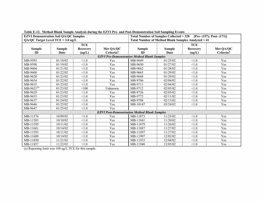
Table E-12. Method Blank Sample Analysis during the EZVI Pre- and Post-Demonstration Soil Sampling Events EZVI Demonstration Soil QA/QC Samples QA/QC Target Level TCE < 3.0 ug/L

Total Number of Samples Collected = 328 [Pre- (157); Post- (171)] Total Number of Method Blank Samples Analyzed = 41

Sample ID

Sample Date

TCE Recovery

(ug/L) Met QA/QC

Criteria? Sample

ID Sample

Date

TCE Recovery

(ug/L) Met QA/QC

Criteria? EZVI Pre-Demonstration Method Blank Samples

MB-9593 01/18/02 <1.0 Yes MB-9649 01/25/02 <1.0 Yes MB-9598 01/19/02 <1.0 Yes MB-9650 01/27/02 <1.0 Yes MB-9604 01/21/02 <1.0 Yes MB-9662 01/28/02 <1.0 Yes MB-9608 01/22/02 <1.0 Yes MB-9665 01/29/02 <1.0 Yes MB-9620 01/23/02 <1.0 Yes MB-9668 01/29/02 <1.0 Yes MB-9634 01/22/02 <1.0 Yes MB-9706 02/04/02 <1.0 Yes MB-9635 01/23/02 <1.0 Yes MB-9711 02/04/02 <1.0 Yes MB-9621(a) 01/23/02 <100 Unknown MB-9712 02/05/02 <1.0 Yes MB-9629 01/23/02 <1.0 Yes MB-9726 02/05/02 <1.0 Yes MB-9635 01/23/02 <1.0 Yes MB-9772 02/11/02 <1.0 Yes MB-9637 01/24/02 <1.0 Yes MB-9788 02/13/02 <1.0 Yes MB-9646 01/25/02 <1.0 Yes MB-10147 03/24/02 <1.0 Yes MB-9647 01/25/02 <1.0 Yes

EZVI Post-Demonstration Method Blank Samples MB-11576 10/09/02 <1.0 Yes MB-11873 11/25/02 <1.0 Yes MB-11583 10/10/02 <1.0 Yes MB-11841 11/20/02 <1.0 Yes MB-11595 10/11/02 <1.0 Yes MB-11879 11/26/02 <1.0 Yes MB-11601 10/14/02 <1.0 Yes MB-11887 11/27/02 <1.0 Yes MB-11593 10/11/02 <1.0 Yes MB-11897 11/27/02 <1.0 Yes MB-11600 10/14/02 <1.0 Yes MB-11907 12/02/02 <1.0 Yes MB-11850 11/21/02 <1.0 Yes MB-11933 12/04/02 <1.0 Yes MB-11857 11/22/02 <1.0 Yes MB-11940 12/05/02 <1.0 Yes (a) Reporting limit was 100 ug/L TCE for this sample.

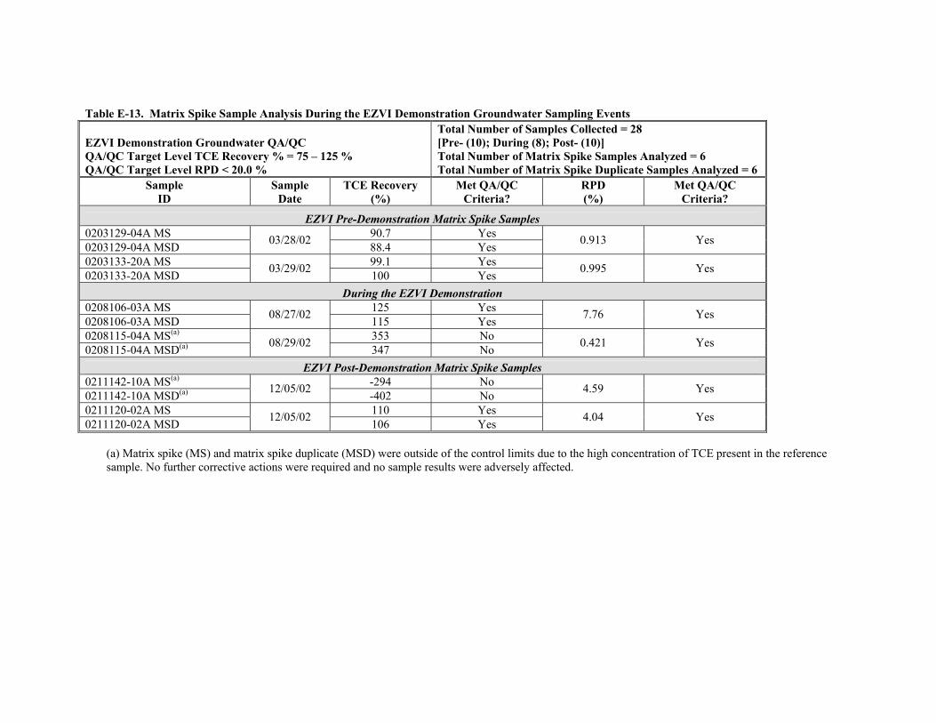
Table E-13. Matrix Spike Sample Analysis During the EZVI Demonstration Groundwater Sampling Events

EZVI Demonstration Groundwater QA/QC QA/QC Target Level TCE Recovery % = 75 – 125 % QA/QC Target Level RPD < 20.0 %

Total Number of Samples Collected = 28 [Pre- (10); During (8); Post- (10)] Total Number of Matrix Spike Samples Analyzed = 6 Total Number of Matrix Spike Duplicate Samples Analyzed = 6

Sample ID

Sample Date

TCE Recovery (%)

Met QA/QC Criteria?

RPD (%)

Met QA/QC Criteria?

EZVI Pre-Demonstration Matrix Spike Samples 0203129-04A MS 03/28/02 90.7 Yes 0.913 Yes0203129-04A MSD 88.4 Yes 0203133-20A MS 03/29/02 99.1 Yes 0.995 Yes0203133-20A MSD 100 Yes

During the EZVI Demonstration 0208106-03A MS 08/27/02 125 Yes 7.76 Yes0208106-03A MSD 115 Yes 0208115-04A MS(a)

08/29/02 353 No 0.421 Yes0208115-04A MSD(a) 347 No EZVI Post-Demonstration Matrix Spike Samples

0211142-10A MS(a)12/05/02 -294 No 4.59 Yes0211142-10A MSD(a) -402 No

0211120-02A MS 12/05/02 110 Yes 4.04 Yes0211120-02A MSD 106 Yes

(a) Matrix spike (MS) and matrix spike duplicate (MSD) were outside of the control limits due to the high concentration of TCE present in the reference sample. No further corrective actions were required and no sample results were adversely affected.

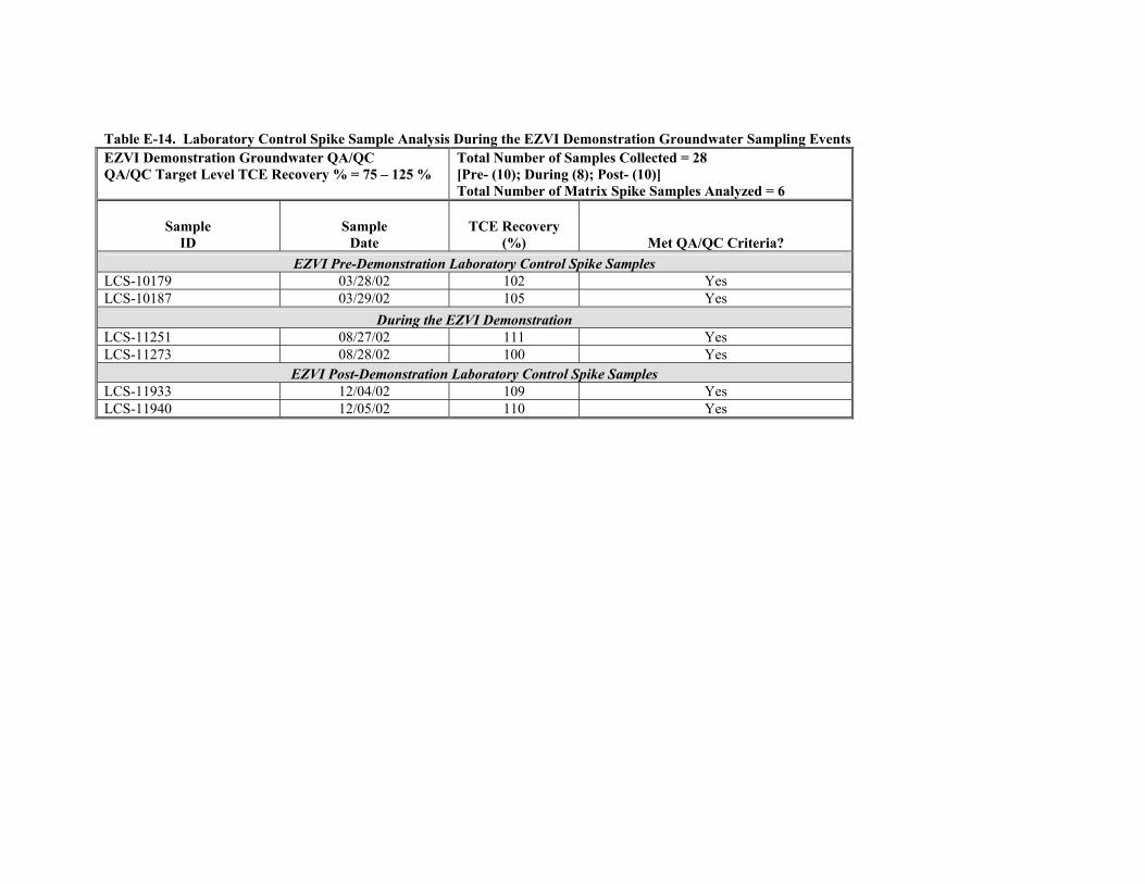
Table E-14. Laboratory Control Spike Sample Analysis During the EZVI Demonstration Groundwater Sampling Events EZVI Demonstration Groundwater QA/QC QA/QC Target Level TCE Recovery % = 75 – 125 %

Total Number of Samples Collected = 28 [Pre- (10); During (8); Post- (10)] Total Number of Matrix Spike Samples Analyzed = 6

Sample ID

Sample Date

TCE Recovery (%) Met QA/QC Criteria?

EZVI Pre-Demonstration Laboratory Control Spike Samples LCS-10179 03/28/02 102 Yes LCS-10187 03/29/02 105 Yes

During the EZVI Demonstration LCS-11251 08/27/02 111 Yes LCS-11273 08/28/02 100 Yes

EZVI Post-Demonstration Laboratory Control Spike Samples LCS-11933 12/04/02 109 Yes LCS-11940 12/05/02 110 Yes

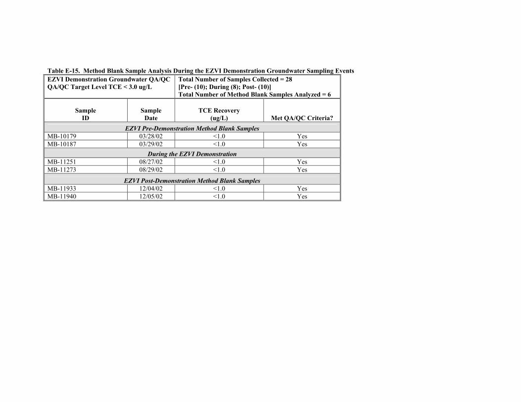
Table E-15. Method Blank Sample Analysis During the EZVI Demonstration Groundwater Sampling Events EZVI Demonstration Groundwater QA/QC QA/QC Target Level TCE < 3.0 ug/L

Total Number of Samples Collected = 28 [Pre- (10); During (8); Post- (10)] Total Number of Method Blank Samples Analyzed = 6

Sample ID

Sample Date

TCE Recovery (ug/L) Met QA/QC Criteria?

EZVI Pre-Demonstration Method Blank Samples MB-10179 03/28/02 <1.0 Yes MB-10187 03/29/02 <1.0 Yes

During the EZVI Demonstration MB-11251 08/27/02 <1.0 Yes MB-11273 08/29/02 <1.0 Yes

EZVI Post-Demonstration Method Blank Samples MB-11933 12/04/02 <1.0 Yes MB-11940 12/05/02 <1.0 Yes

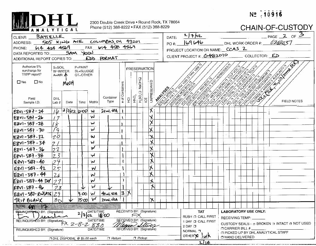
Appendix F

Economic Analysis Information

Table F-1. Pump-and-Treat (P&T) System Design Basis Table F-2. Capital Investment for a P&T System Table F-3. Present Value of P&T System Costs for 30 Years of Operation Table F-4. Present Value of P&T System Costs for 100 Years of Operation Figure F-1. P&T System Costs for 100 Years

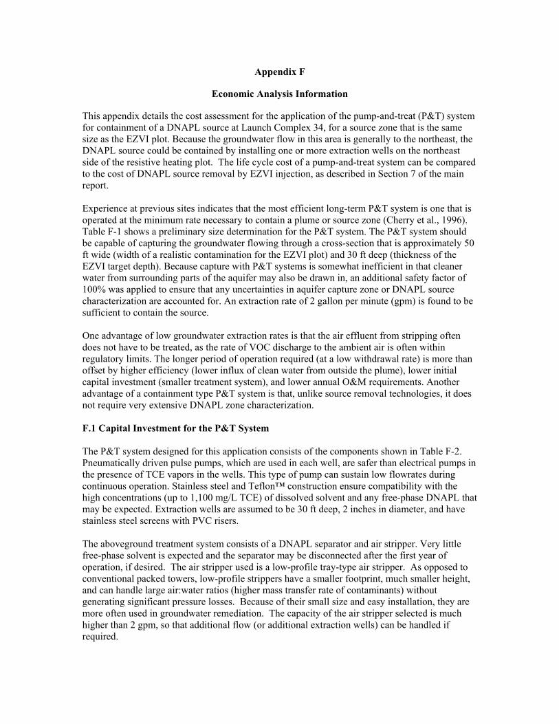
Appendix F

Economic Analysis Information

This appendix details the cost assessment for the application of the pump-and-treat (P&T) system for containment of a DNAPL source at Launch Complex 34, for a source zone that is the same size as the EZVI plot. Because the groundwater flow in this area is generally to the northeast, the DNAPL source could be contained by installing one or more extraction wells on the northeast side of the resistive heating plot. The life cycle cost of a pump-and-treat system can be compared to the cost of DNAPL source removal by EZVI injection, as described in Section 7 of the main report.

Experience at previous sites indicates that the most efficient long-term P&T system is one that is operated at the minimum rate necessary to contain a plume or source zone (Cherry et al., 1996). Table F-1 shows a preliminary size determination for the P&T system. The P&T system should be capable of capturing the groundwater flowing through a cross-section that is approximately 50 ft wide (width of a realistic contamination for the EZVI plot) and 30 ft deep (thickness of the EZVI target depth). Because capture with P&T systems is somewhat inefficient in that cleaner water from surrounding parts of the aquifer may also be drawn in, an additional safety factor of 100% was applied to ensure that any uncertainties in aquifer capture zone or DNAPL source characterization are accounted for. An extraction rate of 2 gallon per minute (gpm) is found to be sufficient to contain the source.

One advantage of low groundwater extraction rates is that the air effluent from stripping often does not have to be treated, as the rate of VOC discharge to the ambient air is often within regulatory limits. The longer period of operation required (at a low withdrawal rate) is more than offset by higher efficiency (lower influx of clean water from outside the plume), lower initial capital investment (smaller treatment system), and lower annual O&M requirements. Another advantage of a containment type P&T system is that, unlike source removal technologies, it does not require very extensive DNAPL zone characterization.

F.1 Capital Investment for the P&T System

The P&T system designed for this application consists of the components shown in Table F-2. Pneumatically driven pulse pumps, which are used in each well, are safer than electrical pumps in the presence of TCE vapors in the wells. This type of pump can sustain low flowrates during continuous operation. Stainless steel and Teflon™ construction ensure compatibility with the high concentrations (up to 1,100 mg/L TCE) of dissolved solvent and any free-phase DNAPL that may be expected. Extraction wells are assumed to be 30 ft deep, 2 inches in diameter, and have stainless steel screens with PVC risers.

The aboveground treatment system consists of a DNAPL separator and air stripper. Very little free-phase solvent is expected and the separator may be disconnected after the first year of operation, if desired. The air stripper used is a low-profile tray-type air stripper. As opposed to conventional packed towers, low-profile strippers have a smaller footprint, much smaller height, and can handle large air:water ratios (higher mass transfer rate of contaminants) without generating significant pressure losses. Because of their small size and easy installation, they are more often used in groundwater remediation. The capacity of the air stripper selected is much higher than 2 gpm, so that additional flow (or additional extraction wells) can be handled if required.

The high air:water ratio ensures that TCE (and other minor volatile components) are removed to the desired levels. The treated water effluent from the air stripper is discharged to the sewer. The air effluent is treated with a catalytic oxidation unit before discharge.

The piping from the wells to the air stripper is run through a 1-ft-deep covered trench. The air stripper and other associated equipment are housed on a 20-ft-x-20-ft concrete pad, covered by a basic shelter. The base will provide a power drop (through a pole transformer) and a licensed electrician will be used for the power hookups. Meters and control valves are strategically placed to control water and air flow through the system.

The existing monitoring system at the site will have to be supplemented with seven long-screen (10-foot screen) monitoring wells. The objective of these wells is to ensure that the desired containment is being achieved.

F.2 Annual Cost of the P&T System

The annual costs of P&T are shown in Table F-3 and include annual O&M. Annual O&M costs include the labor, materials, energy, and waste disposal cost of operating the system and routine maintenance (including scheduled replacement of seals, gaskets, and O-rings). Routine monitoring of the stripper influent and effluent is done through ports on the feed and effluent lines on a monthly basis. Groundwater monitoring is conducted on a quarterly basis through seven monitoring wells. All water samples are analyzed for PCE and other CVOC by-products.

F.3 Periodic Maintenance Cost

In addition to the routine maintenance described above, periodic maintenance will be required, as shown in Table F-3, to replace worn-out equipment. Based on manufacturers’ recommendations for the respective equipment, replacement is done once in 5 or 10 years. In general, all equipment involving moving parts is assumed will be replaced once every 5 years, whereas other equipment is changed every 10 years.

F.4 Present Value (PV) Cost of P&T

Because a P&T system is operated for the long term, a 30-year period of operation is assumed for estimating cost. Because capital investment, annual costs, and periodic maintenance costs occur at different points in time, a life cycle analysis or present value analysis is conducted to estimate the long-term cost of P&T in today’s dollars. This life cycle analysis approach is recommended for long-term remediation applications by the guidance provided in the Federal Technologies Roundtable’s Guide to Documenting and Managing Cost and Performance Information for Remediation Projects (United States Environmental Protection Agency [U.S. EPA], 1998). The PV cost can then be compared with the cost of faster (DNAPL source reduction) remedies.

PV P&T costs = ∑ Annual Cost in Year t Equation (F-1) (1 + r)t

PV P&T costs = Capital Investment + Annual cost in Year 1 + … + Annual cost in Year n (1 + r)1 (1 + r )n

Equation (F-2)

Table F-3 shows the PV calculation for P&T based on Equation F-1. In Equation F-1, each year’s cost is divided by a discount factor that reflects the rate of return that is foregone by incurring the cost. As seen in Equation F-2, at time t = 0, which is in the present, the cost incurred is the initial capital investment in equipment and labor to design, procure, and build the P&T system. Every year after that, a cost is incurred to operate and maintain the P&T system. A real rate of return (or discount rate), r, of 2.9% is used in the analysis as per recent U.S. EPA guidance on discount rates (U.S. EPA, 1999). The total PV cost of purchasing, installing, and operating a 2-gpm P&T source containment system for 30 years is estimated to be $1,360,000 (rounded to the nearest thousand).

Long-term remediation costs are typically estimated for 30-year periods as mentioned above. Although the DNAPL source may persist for a much longer time, the contribution of costs incurred in later years to the PV cost of the P&T system is not very significant and the total 30-year cost is indicative of the total cost incurred for this application. This can be seen from the fact that in Years 28, 29, and 30, the differences in cumulative PV cost are not as significant as the difference in, say, Years 2, 3, and 4. The implication is that, due to the effect of discounting, costs that can be postponed to later years have a lower impact than costs that are incurred in the present.

As an illustration of a DNAPL source that may last much longer than the 30-year period of calculation, Figure F-1 shows a graphic representation of PV costs assuming that the same P&T system is operated for 100 years instead of 30 years. The PV cost curve flattens with each passing year. The total PV cost after 100 years (in Table F-4) is estimated at $2,126,000.

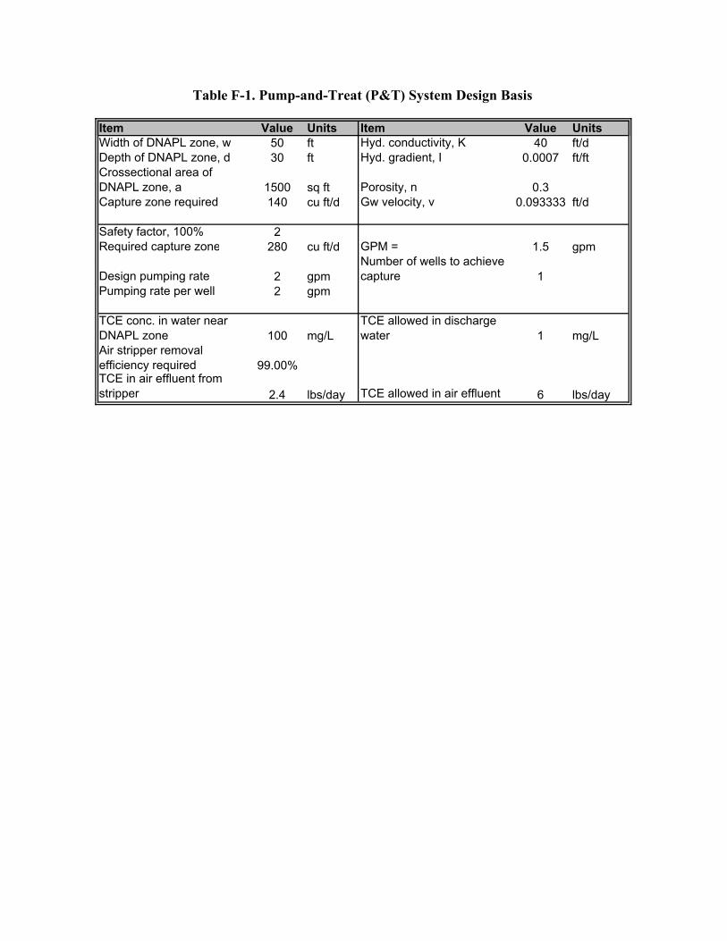
Item Value Units Item Value Units Width of DNAPL zone, w Depth of DNAPL zone, d Crossectional area of

50 30

ft ft

Hyd. conductivity, K Hyd. gradient, I

40 ft/d 0.0007 ft/ft

DNAPL zone, a Capture zone required

1500 140

sq ft cu ft/d

Porosity, n Gw velocity, v

0.3 0.093333 ft/d

Safety factor, 100% Required capture zone

2 280 cu ft/d GPM =

Number of wells to achieve 1.5 gpm

Design pumping rate Pumping rate per well

2 2

gpm gpm

capture 1

TCE conc. in water near DNAPL zone Air stripper removal efficiency required TCE in air effluent from

100

99.00%

mg/L TCE allowed in discharge water 1 mg/L

stripper 2.4 lbs/day TCE allowed in air effluent 6 lbs/day

Table F-1. Pump-and-Treat (P&T) System Design Basis

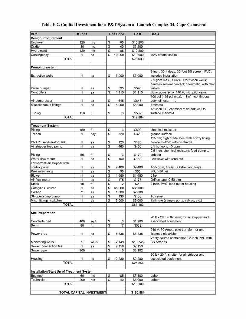
Table F-2. Capital Investment for a P&T System at Launch Complex 34, Cape Canaveral

Item # units Unit Price Cost Basis Design/Procurement Engineer 120 hrs 85$ $10,200 Drafter 80 hrs 40$ $3,200 Hydrologist 120 hrs 85$ $10,200 Contingency 1 ea 10,000$ $10,000 10% of total capital

TOTAL $23,600

Pumping system

Extraction wells 1 ea 5,000$ $5,000 2-inch, 30 ft deep, 30-foot SS screen; PVC; includes installation

Pulse pumps 1 ea 595$ $595

2.1 gpm max., 1.66"OD for 2-inch wells; handles solvent contact; pneumatic; with chec valves

Controllers 1 ea 1,115$ $1,115 Solar powered or 110 V; with pilot valve

Air compressor 1 ea 645$ $645 100 psi (125 psi max), 4.3 cfm continuous duty, oil-less; 1 hp

Miscellaneous fittings 1 ea 5,000$ $5,000 Estimate

Tubing 150 ft 3$ $509 1/2-inch OD, chemical resistant; well to surface manifold

TOTAL $12,864

Treatment System Piping 150 ft 3$ $509 chemical resistant Trench 1 day 320$ $320 ground surface

DNAPL separarator tank 1 ea 120$ $120 125 gal; high grade steel with epoxy lining; conical bottom with discharge

Air stripper feed pump 1 ea 460$ $460 0.5 hp; up to 15 gpm

Piping 50 ft 3$ $170 0.5 inch, chemical resistant; feed pump to stripper

Water flow meter 1 ea 160$ $160 Low flow; with read out Low-profile air stripper with control panel 1 ea 9,400$ $9,400 1-25 gpm, 4 tray; SS shell and trays Pressure gauge 1 ea 50 $ $50 SS; 0-30 psi Blower 1 ea 1,650$ $1,650 5 hp Air flow meter 1 ea 175$ $175 Orifice type; 0-50 cfm Stack 10 ft 2$ $20 2 inch, PVC, lead out of housing Catalytic Oxidizer 1 ea 65,000$ $65,000 Carbon 2 ea 1,000$ $2,000 Stripper sump pump 1 ea 130$ $130 To sewer Misc. fittings, switches 1 ea 5,000$ $5,000 Estimate (sample ports, valves, etc.)

TOTAL $85,163

Site Preparation

Conctrete pad 400 sq ft 3$ $1,200 20 ft x 20 ft with berm; for air stripper and associated equipment

Berm 80 ft 7$ $539

Power drop 1 ea 5,838$ $5,838 240 V, 50 Amps; pole transformer and licensed electrician

Monitoring wells 5 wells 2,149$ $10,745 Verify source containment; 2-inch PVC with SS screens

Sewer connection fee 1 ea 2,150$ $2,150 Sewer pipe 300 ft 10$ $3,102

Housing 1 ea 2,280$ $2,280 20 ft x 20 ft; shelter for air stripper and associated equipment

TOTAL $25,854

Installation/Start Up of Treatment System Engineer 60 hrs 85$ $5,100 Labor Technician 200 hrs 40$ $8,000 Labor

TOTAL $13,100

TOTAL CAPITAL INVESTMENT $160,581

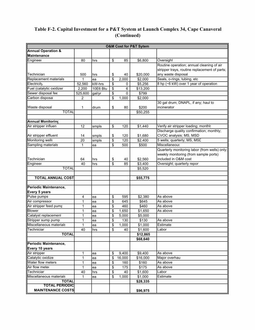
Table F-2. Capital Investment for a P&T System at Launch Complex 34, Cape Canaveral (Continued)

O&M Cost for P&T Sytem Annual Operation & Maintenance Engineer 80 hrs 85$ $6,800 Oversight

Technician 500 hrs 40$ $20,000

Routine operation; annual cleaning of air stripper trays, routine replacement of parts; any waste disposal

Replacement materials 1 ea 2,000$ $2,000 Seals, o-rings, tubing, etc. Electricity 52,560 kW-hrs 0$ $5,256 8 hp (~6 kW) over 1 year of operation Fuel (catalytic oxidizer 2,200 10E6 Btu 6$ $13,200 Sewer disposal fee 525,600 gal/yr 0$ $799 Carbon disposal 2 1,000$ $2,000

Waste disposal 1 drum 80$ $200 30 gal drum; DNAPL, if any; haul to incinerator

TOTAL $50,255

Annual Monitoring Air stripper influent 12 smpls 120$ $1,440 Verify air stripper loading; monthly

Air stripper effluent 14 smpls 120$ $1,680 Discharge quality confirmation; monthly; CVOC analysis; MS, MSD

Monitoring wells 20 smpls 120$ $2,400 5 wells; quarterly; MS, MSD Sampling materials 1 ea 500$ $500 Miscellaneous

Technician 64 hrs 40$ $2,560

Quarterly monitoring labor (from wells) only; weekly monitoring (from sample ports) included in O&M cost

Engineer 40 hrs 85$ $3,400 Oversight; quarterly report TOTAL $5,520

TOTAL ANNUAL COST $55,775

Periodic Maintenance, Every 5 years Pulse pumps 4 ea 595$ $2,380 As above Air compressor 1 ea 645$ $645 As above Air stripper feed pump 1 ea 460$ $460 As above Blower 1 ea 1,650$ $1,650 As above Catalyst replacement 1 ea 5,000$ $5,000 Stripper sump pump 1 ea 130$ $130 As above Miscellaneous materials 1 ea 1,000$ $1,000 Estimate Technician 40 hrs 40$ $1,600 Labor

TOTAL $12,865 $68,640

Periodic Maintenance, Every 10 years Air stripper 1 ea 9,400$ $9,400 As above Catalytic oxidizer 1 ea 16,000$ $16,000 Major overhaul Water flow meters 1 ea 160$ $160 As above Air flow meter 1 ea 175$ $175 As above Technician 40 hrs 40$ $1,600 Labor Miscellaneous materials 1 ea 1,000$ $1,000 Estimate

TOTAL $28,335 TOTAL PERIODIC

MAINTENANCE COSTS $96,975

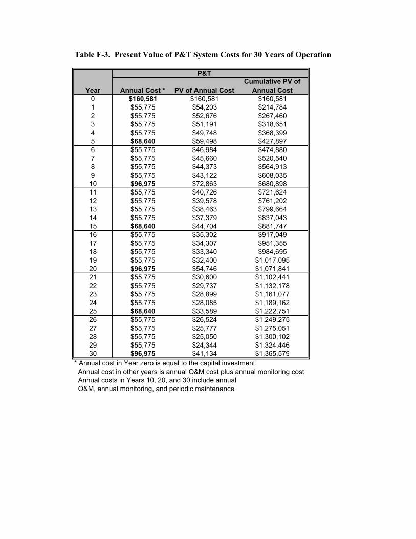
Table F-3. Present Value of P&T System Costs for 30 Years of Operation

Year

P&T

Annual Cost * PV of Annual Cost Cumulative PV of

Annual Cost 0 1 2 3 4 5

$160,581 $55,775 $55,775 $55,775 $55,775 $68,640

$160,581 $54,203 $52,676 $51,191 $49,748 $59,498

$160,581 $214,784 $267,460 $318,651 $368,399 $427,897

6 7 8 9 10

$55,775 $55,775 $55,775 $55,775 $96,975

$46,984 $45,660 $44,373 $43,122 $72,863

$474,880 $520,540 $564,913 $608,035 $680,898

11 12 13 14 15

$55,775 $55,775 $55,775 $55,775 $68,640

$40,726 $39,578 $38,463 $37,379 $44,704

$721,624 $761,202 $799,664 $837,043 $881,747

16 17 18 19 20

$55,775 $55,775 $55,775 $55,775 $96,975

$35,302 $34,307 $33,340 $32,400 $54,746

$917,049 $951,355 $984,695

$1,017,095 $1,071,841

21 22 23 24 25

$55,775 $55,775 $55,775 $55,775 $68,640

$30,600 $29,737 $28,899 $28,085 $33,589

$1,102,441 $1,132,178 $1,161,077 $1,189,162 $1,222,751

26 27 28 29 30

$55,775 $55,775 $55,775 $55,775 $96,975

$26,524 $25,777 $25,050 $24,344 $41,134

$1,249,275 $1,275,051 $1,300,102 $1,324,446 $1,365,579

* Annual cost in Year zero is equal to the capital investment. Annual cost in other years is annual O&M cost plus annual monitoring cost Annual costs in Years 10, 20, and 30 include annual O&M, annual monitoring, and periodic maintenance

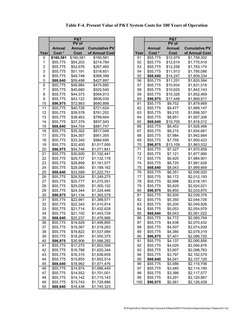
Table F-4. Present Value of P&T System Costs for 100 Years of Operation

P&T PV of

Annual Annual Cumulative PV Year Cost * Cost of Annual Cost

0 $160,581 $160,581 $160,581 1 $55,775 $54,203 $214,784 2 $55,775 $52,676 $267,460 3 $55,775 $51,191 $318,651 4 $55,775 $49,748 $368,399 5 $68,640 $59,498 $427,897 6 $55,775 $46,984 $474,880 7 $55,775 $45,660 $520,540 8 $55,775 $44,373 $564,913 9 $55,775 $43,122 $608,035 10 $96,975 $72,863 $680,898 11 $55,775 $40,726 $721,624 12 $55,775 $39,578 $761,202 13 $55,775 $38,463 $799,664 14 $55,775 $37,379 $837,043 15 $68,640 $44,704 $881,747 16 $55,775 $35,302 $917,049 17 $55,775 $34,307 $951,355 18 $55,775 $33,340 $984,695 19 $55,775 $32,400 $1,017,095 20 $96,975 $54,746 $1,071,841 21 $55,775 $30,600 $1,102,441 22 $55,775 $29,737 $1,132,178 23 $55,775 $28,899 $1,161,077 24 $55,775 $28,085 $1,189,162 25 $68,640 $33,589 $1,222,751 26 $55,775 $26,524 $1,249,275 27 $55,775 $25,777 $1,275,051 28 $55,775 $25,050 $1,300,102 29 $55,775 $24,344 $1,324,446 30 $96,975 $41,134 $1,365,579 31 $55,775 $22,991 $1,388,571 32 $55,775 $22,343 $1,410,914 33 $55,775 $21,714 $1,432,628 34 $55,775 $21,102 $1,453,729 35 $68,640 $25,237 $1,478,966 36 $55,775 $19,929 $1,498,895 37 $55,775 $19,367 $1,518,263 38 $55,775 $18,822 $1,537,084 39 $55,775 $18,291 $1,555,375 40 $96,975 $30,906 $1,586,282 41 $55,775 $17,275 $1,603,556 42 $55,775 $16,788 $1,620,344 43 $55,775 $16,315 $1,636,659 44 $55,775 $15,855 $1,652,514 45 $68,640 $18,962 $1,671,476 46 $55,775 $14,974 $1,686,449 47 $55,775 $14,552 $1,701,001 48 $55,775 $14,142 $1,715,143 49 $55,775 $13,743 $1,728,886 50 $68,640 $16,436 $1,745,323

P&T PV of

Annual Annual Cumulative PV Year Cost * Cost of Annual Cost 51 $55,775 $12,979 $1,758,302 52 $55,775 $12,614 $1,770,916 53 $55,775 $12,258 $1,783,174 54 $55,775 $11,913 $1,795,086 55 $68,640 $14,247 $1,809,334 56 $55,775 $11,251 $1,820,584 57 $55,775 $10,934 $1,831,518 58 $55,775 $10,625 $1,842,143 59 $55,775 $10,326 $1,852,469 60 $96,975 $17,448 $1,869,917 61 $55,775 $9,752 $1,879,669 62 $55,775 $9,477 $1,889,147 63 $55,775 $9,210 $1,898,357 64 $55,775 $8,951 $1,907,308 65 $68,640 $10,705 $1,918,012 66 $55,775 $8,453 $1,926,466 67 $55,775 $8,215 $1,934,681 68 $55,775 $7,984 $1,942,664 69 $55,775 $7,759 $1,950,423 70 $96,975 $13,109 $1,963,532 71 $55,775 $7,327 $1,970,859 72 $55,775 $7,121 $1,977,980 73 $55,775 $6,920 $1,984,901 74 $55,775 $6,725 $1,991,626 75 $68,640 $8,043 $1,999,669 76 $55,775 $6,351 $2,006,020 77 $55,775 $6,172 $2,012,193 78 $55,775 $5,998 $2,018,191 79 $55,775 $5,829 $2,024,021 80 $96,975 $9,850 $2,033,870 81 $55,775 $5,505 $2,039,376 82 $55,775 $5,350 $2,044,726 83 $55,775 $5,200 $2,049,926 84 $55,775 $5,053 $2,054,979 85 $68,640 $6,043 $2,061,022 86 $55,775 $4,772 $2,065,794 87 $55,775 $4,638 $2,070,432 88 $55,775 $4,507 $2,074,939 89 $55,775 $4,380 $2,079,319 90 $96,975 $7,401 $2,086,720 91 $55,775 $4,137 $2,090,856 92 $55,775 $4,020 $2,094,876 93 $55,775 $3,907 $2,098,783 94 $55,775 $3,797 $2,102,579 95 $68,640 $4,541 $2,107,120 96 $55,775 $3,586 $2,110,706 97 $55,775 $3,485 $2,114,190 98 $55,775 $3,386 $2,117,577 99 $55,775 $3,291 $2,120,867 100 $96,975 $5,561 $2,126,428

M:\Projects\Envir Restor\Cape Canaveral 2\Reports\EZVI Post-Demo\Appendices\App F\Appendix F.xls

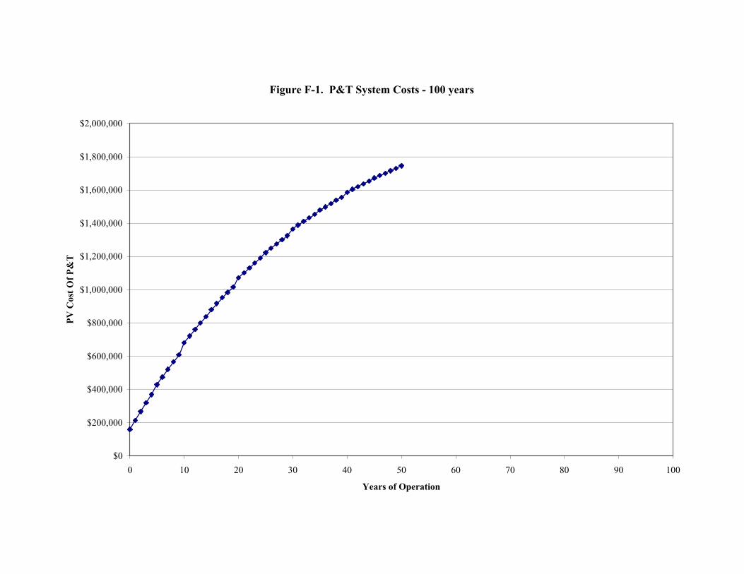
Figure F-1. P&T System Costs - 100 years

$0

$200,000

$400,000

$600,000

$800,000

$1,000,000

$1,200,000

$1,400,000

$1,600,000

$1,800,000

$2,000,000

PV C

ost O

f P&

T

0 10 20 30 40 50 60 70 80 90

Years of Operation

100