updating florda department of transportation's...
TRANSCRIPT

UPDATING FLORIDA DEPARTMENT OF TRANSPORTATION'S (FDOT) PILE/SHAFT DESIGN PROCEDURES BASED ON CPT & DTP DATA
By
ZHIHONG HU
A DISSERTATION PRESENTED TO THE GRADUATE SCHOOL OF THE UNIVERSITY OF FLORIDA IN PARTIAL FULFILLMENT
OF THE REQUIREMENTS FOR THE DEGREE OF DOCTOR OF PHILOSOPHY
UNIVERSITY OF FLORIDA
2007
1

© 2007 Zhihong Hu
2

To my wife for her strong support, endless encouragement, and help to make this happen
3

ACKNOWLEDGMENTS
I first thank to my wife, Meiyu, for her endless support, advice, and encouragement of my
research and my dissertation. Without her support, this dissertation could not be finished. I
would also like to thank to my parents, who also encouraged me to finish my study and work.
I want to say thank you for Dr. Bloomquist for his innovate ideas, helpful advice, and
guidance to fulfill this dissertation. I also want to thank to Dr. McVay for his insight,
knowledge, patient discussions, suggestions, and good research model. There are also many
other professors who devoted time and energy to my research, such as Dr. Townsend, Dr.
Hiltunen, Dr. Consolazio and Dr. Flood. I would like to thank them, as well.
Finally, I would like to thank to my classmates, Jeongsoo Ko, Scott Wasman, Patrick
Dunn, Luis Campos, Adrian Viala, Heath Forbes, and Mark Styler. Thank you for your help
with my research.
4

TABLE OF CONTENTS page
ACKNOWLEDGMENTS ...............................................................................................................4
LIST OF TABLES...........................................................................................................................7
LIST OF FIGURES .........................................................................................................................8
ABSTRACT...................................................................................................................................15
CHAPTER
1 INTRODUCTION ..................................................................................................................17
2 LITERATURE REVIEW .......................................................................................................20
Cemented Sand .......................................................................................................................20 Cone Penetration Test (CPT)..................................................................................................23 CPT Based Pile Capacity Prediction Methods .......................................................................25
Schmertmann Method .....................................................................................................26 De Ruiter and Beringen Method......................................................................................27 Penpile Method................................................................................................................28 Prince and Wardle Method..............................................................................................28 Tumay and Fakhroo Method ...........................................................................................29 Aoki and De Alencar Method..........................................................................................29 Philipponnat Method .......................................................................................................30 LCPC (Bustamante and Gianeselli) Method ...................................................................30 Almeida et al. Method .....................................................................................................30 MTD (Jardine and Chow) Method ..................................................................................31 Eslami and Fellenius Method ..........................................................................................35 Powell et al. Method........................................................................................................36 UWA-05 Method.............................................................................................................37 Zhou et al. Method ..........................................................................................................38
3 MATERIALS AND METHODS ...........................................................................................41
Dual Tip Penetrometer (DTP) ................................................................................................41 Locate Cemented Sites ...........................................................................................................42 Axial Ultimate Pile Capacity Prediction Methods..................................................................42 Load and Resistance Factor Design (LRFD)..........................................................................43
Modified First Order Second Moment (FOSM) Approach.............................................43 Limit state equation..................................................................................................44 Reliability index .......................................................................................................45 Resistance factor Φ ..................................................................................................45
Differentiate Ultimate Skin Friction and Tip Resistance from Load Test Data .....................49 The Proposed UF Method.......................................................................................................51
5
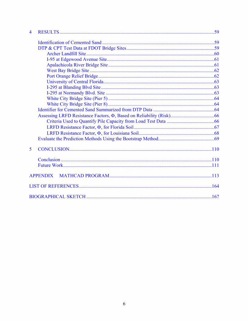
4 RESULTS...............................................................................................................................59
Identification of Cemented Sand ............................................................................................59 DTP & CPT Test Data at FDOT Bridge Sites........................................................................59
Archer Landfill Site .........................................................................................................60 I-95 at Edgewood Avenue Site........................................................................................61 Apalachicola River Bridge Site .......................................................................................61 West Bay Bridge Site ......................................................................................................62 Port Orange Relief Bridge ...............................................................................................62 University of Central Florida...........................................................................................63 I-295 at Blanding Blvd Site .............................................................................................63 I-295 at Normandy Blvd. Site .........................................................................................63 White City Bridge Site (Pier 5) .......................................................................................64 White City Bridge Site (Pier 8) .......................................................................................64
Identifier for Cemented Sand Summarized from DTP Data ..................................................64 Assessing LRFD Resistance Factors, Φ, Based on Reliability (Risk)....................................66
Criteria Used to Quantify Pile Capacity from Load Test Data .......................................66 LRFD Resistance Factor, Φ, for Florida Soil..................................................................67 LRFD Resistance Factor, Φ, for Louisiana Soil..............................................................68
Evaluate the Prediction Methods Using the Bootstrap Method..............................................69
5 CONCLUSION.....................................................................................................................110
Conclusion ............................................................................................................................110 Future Work..........................................................................................................................111
APPENDIX MATHCAD PROGRAM....................................................................................113
LIST OF REFERENCES.............................................................................................................164
BIOGRAPHICAL SKETCH .......................................................................................................167
6

LIST OF TABLES
Table page 3-1 Ultimate unit tip resistance factor k b .................................................................................53
3-2 Ultimate unit skin friction empirical factor, Fs ..................................................................53
4-1 Predicted ultimate skin friction for 14 CPT methods (Florida soil) ..................................71
4-2 Predicted ultimate tip resistance for 14 CPT methods (Florida soil).................................72
4-3 Predicted Davisson capacity for 14 CPT methods (Florida soil).......................................73
4-4 LRFD resistance factors,Φ, for CPT methods (ultimate skin friction, Florida soil)..........74
4-5 LRFD resistance factors,Φ, for CPT methods (ultimate tip resistance, Florida soil) ........74
4-6 LRFD resistance factors,Φ, for CPT methods (Davisson capacity, Florida soil)..............75
4-7 Predicted ultimate skin friction for 14 CPT methods (Louisiana soil) ..............................76
4-8 Predicted ultimate tip resistance for 14 CPT methods (Louisiana soil).............................77
4-9 Predicted ultimate pile capacity for 14 CPT methods (Louisiana soil) .............................78
4-10 LRFD resistance factors,Φ, for CPT methods (ultimate skin friction, Louisiana soil) .....79
4-11 LRFD resistance factors,Φ, for CPT methods (ultimate tip resistance, Louisiana soil)....79
4-12 LRFD resistance factors,Φ, for CPT methods (ultimate pile capacity, Louisiana soil) ....80
5-1 Bridge sites where load test data are available ................................................................112
7

LIST OF FIGURES
Figure page 2-1 Regular cone penetrometer ................................................................................................40
3-1 Dual tip penetrometer ........................................................................................................54
3-2 The locations of 21 sites with load test data and CPT data ...............................................55
3-3 MathCAD program for Philipponnat method ....................................................................56
3-4 Static load test, Apalachicola Bay Bridge (pier 3).............................................................57
3-5 Separate the ultimate skin friction and tip resistance.........................................................58
4-1 CPT and DTP test data from Archer Landfill site .............................................................81
4-2 Friction ratio of CPT and DTP rest from Archer Landfill site ..........................................82
4-3 CPT and DTP test data from I–95 at Edgewood Avenue site............................................83
4-4 Friction ratio of CPT and DTP test from I–95 at Edgewood Avenue site.........................84
4-5 Tip2/Tip1 ratio and Qc/N ratio of CPT and DTP test from I–95 at Edgewood Avenue site ......................................................................................................................................85
4-6 CPT and DTP test data from Apalachicola River Bridge site ...........................................86
4-7 Tip2/Tip1 ratio and Qc/N ratio of CPT and DTP test from Apalachicola River Bridge site ......................................................................................................................................87
4-8 CPT and DTP test data from West Bay Bridge site...........................................................88
4-9 Tip2/Tip1 ratio and Qc/N ratio of CPT and DTP test from West Bay Bridge site............89
4-10 CPT and DTP test data from Port Orange Relief Bridge site ............................................90
4-11 Tip2/Tip1 ratio and Qc/N ratio of CPT and DTP test from Port Orange Relief Bridge site ......................................................................................................................................91
4-12 CPT and DTP test data at the University of Central Florida site.......................................92
4-13 Tip2/Tip1 ratio and Qc/N ratio of CPT and DTP test at the University of Central Florida site .........................................................................................................................93
4-14 CPT and DTP test data at I-295 at Blanding Blvd site ......................................................94
4-15 Tip2/Tip1 ratio and Qc/N ratio of CPT and DTP test at I-295 at Blanding Blvd site .......95
8
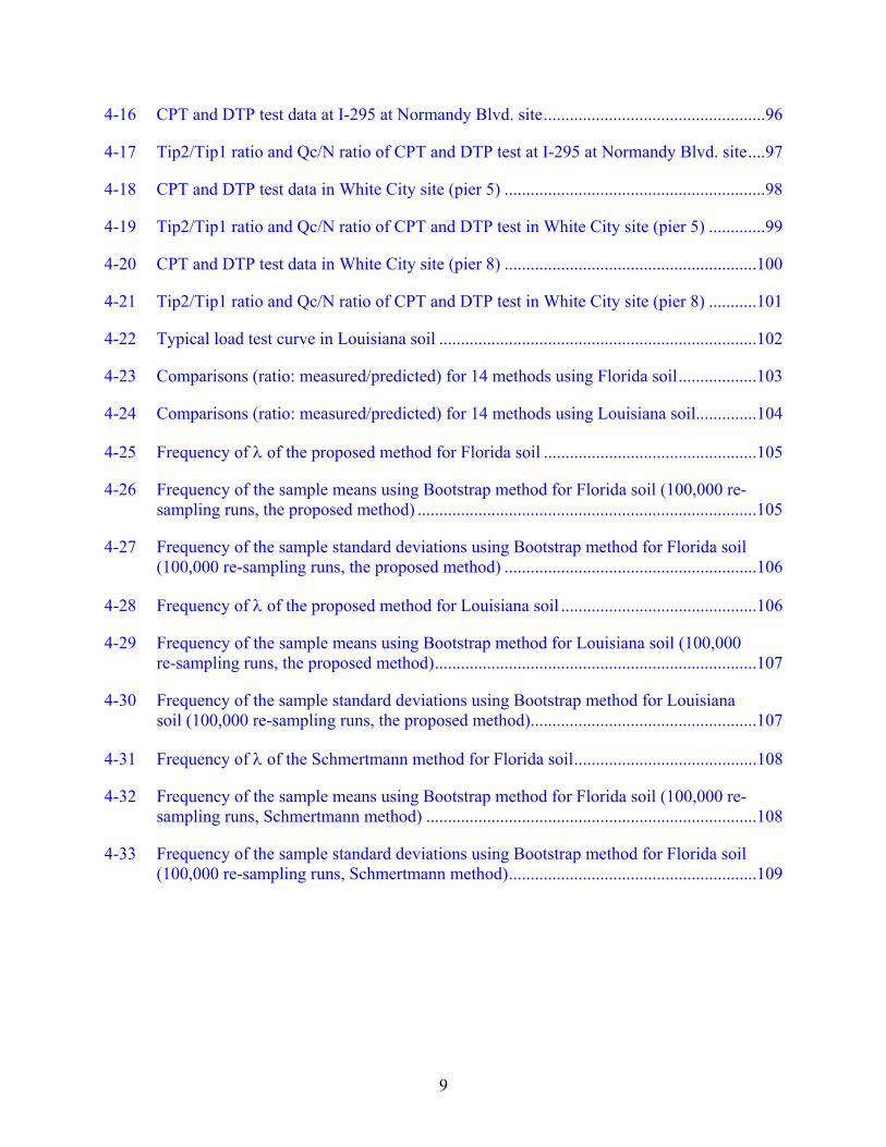
4-16 CPT and DTP test data at I-295 at Normandy Blvd. site...................................................96
4-17 Tip2/Tip1 ratio and Qc/N ratio of CPT and DTP test at I-295 at Normandy Blvd. site....97
4-18 CPT and DTP test data in White City site (pier 5) ............................................................98
4-19 Tip2/Tip1 ratio and Qc/N ratio of CPT and DTP test in White City site (pier 5) .............99
4-20 CPT and DTP test data in White City site (pier 8) ..........................................................100
4-21 Tip2/Tip1 ratio and Qc/N ratio of CPT and DTP test in White City site (pier 8) ...........101
4-22 Typical load test curve in Louisiana soil .........................................................................102
4-23 Comparisons (ratio: measured/predicted) for 14 methods using Florida soil..................103
4-24 Comparisons (ratio: measured/predicted) for 14 methods using Louisiana soil..............104
4-25 Frequency of λ of the proposed method for Florida soil .................................................105
4-26 Frequency of the sample means using Bootstrap method for Florida soil (100,000 re-sampling runs, the proposed method) ..............................................................................105
4-27 Frequency of the sample standard deviations using Bootstrap method for Florida soil (100,000 re-sampling runs, the proposed method) ..........................................................106
4-28 Frequency of λ of the proposed method for Louisiana soil .............................................106
4-29 Frequency of the sample means using Bootstrap method for Louisiana soil (100,000 re-sampling runs, the proposed method)..........................................................................107
4-30 Frequency of the sample standard deviations using Bootstrap method for Louisiana soil (100,000 re-sampling runs, the proposed method)....................................................107
4-31 Frequency of λ of the Schmertmann method for Florida soil..........................................108
4-32 Frequency of the sample means using Bootstrap method for Florida soil (100,000 re-sampling runs, Schmertmann method) ............................................................................108
4-33 Frequency of the sample standard deviations using Bootstrap method for Florida soil (100,000 re-sampling runs, Schmertmann method).........................................................109
9

LIST OF ABBREVIATIONS
α Empirical factor to calculate tip resistance in Zhou et al. method
α C Penetrometer to pile friction ratio in clay in Schmertmann method
α S Penetrometer to pile friction ratio in sand in Schmertmann method
α s Empirical factor to calculate skin friction in Philipponnat method
A S Surface area for the calculation of skin friction
ASTM American society for testing and materials
β Adhesion factor in De Ruiter and Beringen method and Zhou et al. method
βT Target reliability index
C S Pile skin friction factor in Eslami and Fellenius method
CPT Cone penetration test
COV (Q) Load coefficients of variation
COV (R) Resistance coefficient of variation
COVQD Dead load coefficient of variation
COVQL Live load coefficient of variation
δ f Pile-soil interface friction angle at the maxmum shear stress
δcv Constant volume interface friction angle between sand and pile
D Diameter or side length of pile
D CPT Diameter of cone penetrometer
D int The internal diameter for pipe pile
DTP Dual tip penetrometer
∆r Interface dilation
∆σ'rd The net dilatant component
Φ LRFD resistance factor
F b Empirical factor to calculate tip resistance in Aoki and De Alencar method
10

F s Empirical factor to calculate skin friction in Aoki and De Alencar method
F S Empirical factor to calculate skin friction in Philipponnat method
FDOT Florida department of transportation
FORM First Order Reliability method
FOSM First Order Second moment
f L Loading coefficient
f S Pile unit skin friction
f sa Average CPT sleeve friction
φ Friction angle
G The sand shear modulus, failure equation in terms of random variables
G max Maximum shear modulus
γD Dead load factor
γL Live load factor
h The hight above the pile tip
I-295 Interstate 295
I-95 Interstate 95
K c Earth pressure coeffient after equilization
k Pile tip resistance factor in MTD method
k 1 Pile skin friction factor in Almeida et al. method and Powell et al. method
k 2 Pile tip resistance factor in Almeida et al. method and Powell et al. method
k b Pile tip resistance factor in Prince, Wardle method Philipponnat method, LCPC method, and the Proposed method
k S Pile skin friction factor in Prince and Wardle method
L Pile embedment length
LCPC Laboratoire central des ponts et chaussées
11

LRFD Load and resistance factor design
γ i Load factors
λQD Dead load bias factor
λQL Live load bias factor
λR The mean bias
λRi The ratio of measured to predicted pile capacities
MTD Marine technology directorate
MN/m2 Mega Newton per square meters
m Pile skin friction factor in Tumay and Fakhroo method
N The number of cases, or SPT blow count
NC Bearing capacity factor
Nk Cone factor in De Ruiter and Beringen method
N kt Cone factor in Powell et al. method
Ns Cone factor to estimate sensitivity
NCHRP National cooperative highway research program
OCR Over consolidation ratio
PI Plasticity index
Pa The atmosphere pressure
PPC Precast-prestressed-concrete
PL-AID Pile load settlement analysis from in-situ data
psi Pound per square inches
Q Random variable for load
Qc/N The ratio of CPT tip resistance to the SPT blow count
Q I Force effects
QD Dead load
12
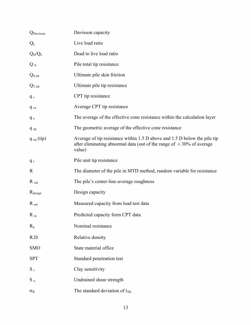
QDavisson Davisson capacity
QL Live load ratio
QD/QL Dead to live load ratio
Q S Pile total tip resistance
QS ult Ultimate pile skin friction
QT ult Ultimate pile tip resistance
q c CPT tip resistance
q ca Average CPT tip resistance
q e The average of the effective cone resistance within the calculation layer
q eg The geometric average of the effective cone resistance
q eq (tip) Average of tip resistance within 1.5 D above and 1.5 D below the pile tip after eliminating abnormal data (out of the range of ± 30% of average value)
q t Pile unit tip resistance
R The diameter of the pile in MTD method, random variable for resistance
R cla The pile’s center-line-average roughness
Rdesign Design capacity
R mi Measured capacity from load test data
R ni Predicted capacity form CPT data
Rn Nominal resistance
R.D. Relative density
SMO State material office
SPT Standard penetration test
S t Clay sensitivity
S u Undrained shear strength
σR The standard deviation of λRi
13

σ'rc Radial effective stress on side after equalization
σ'rf Radial effective stress at maximum shear stress
σ v0 The total overburden stress
σ’v0 The effective overburden stress
T1 DTP first tip resistance
T2 DTP second tip resistance
tsf Tons per square feet
UF The University of Florida
UWA The university of Western Australia
VAR Variance
YSR Yield stress ratio
y The distance between the surface and the skin friction calculating point
η Load modifier for importance, redundancy and ductility
14

Abstract of Dissertation Presented to the Graduate School of the University of Florida in Partial Fulfillment of the Requirements for the Degree of Doctor of Philosophy
UPDATING FLORIDA DEPARTMENT OF TRANSPORTATION'S (FDOT'S) PILE/SHAFT DESIGN PROCEDURES BASED ON CPT & DTP DATA
By
Zhihong Hu
December 2007
Chair: David Bloomquist Cochair: Michael C. McVay Major: Civil Engineering
The Florida Department of Transportation (FDOT) began developing a geotech-material-
construction database that includes information on piles and drilled shafts, specifically, in-situ
data (SPT, CPT, etc.) and load test data in the early 1990s. More recently, FDOT sponsored
novel research to develop a new in-situ device, the dual tip penetrometer (DTP), to identify
cemented soils and thereby contribute to the database data. My research evaluated current pile
design methodologies (Schmertmann, LCPC, etc.) using CPT, DTP, and modified current
methods and proposed a new method to improve future driven pile design. My research also
involves identifying cemented soils using the DTP, since cementation is a critical issue in pile
design procedures.
My research explores 14 pile-capacity-design methods based on cone penetration test
(CPT) and assesses load and resistance factor design (LRFD) resistance factors for each using 21
cases from Florida and 28 from Louisiana. The resulting resistance factors were not satisfactory
for any of the methods. A new design method was proposed, taking into account cementation
and other issues. The LRFD resistance factor was also assessed for this new method. DTP tests
were performed at cemented-soil sites to verify the cemented-soil identification (T2/T1, [Tip
15

1/Tip 2], and Friction Ratio) from DTP. The ratio T2/T1 was finally determined to be an
excellent identifier in locating cemented sand.
My new method provides better LRFD resistance factors for both Florida soil and
Louisiana soils. It could be a promising method to improve pile design in the future. From the
DTP tests in cemented soils, it was concluded that the DTP could be an efficient tool to identify
cemented sand and thereby better predict pile capacity.
16

CHAPTER 1 INTRODUCTION
From the 1960s to the 1980s, FDOT sponsored research at the University of Florida to
evaluate the methods used for calculating static pile capacity based on the CPT (cone penetration
test). After years of research, Dr. John H. Schmertmann (1978) proposed the method which was
later named after him. This method was put into the FDOT pile design software and termed,
PL-AID. This method has been used successfully in the districts of Florida on 16” to 18”
precast-prestressed-concrete (PPC) piles. However, during the last two decades, the size of the
pile has increased to 24” to 30”, primarily due to higher strength concretes and steel as well as
larger pile driving equipment. The Schmertmann method became conservative in evaluating pile
capacity based on the comparison between the predictions and static load test results.
Compare to drilled shaft, driven piles have their own advantages. There are significant
reductions of lateral capacity for drilled shaft due to torsional loading (Hu et al. 2006). Since
driven piles are usually in group and there will be no reduction of lateral capacity due to
torsional loading. That is the reason why more and more CPT based pile capacity prediction
methods have been proposed. During the 1980s, many methods were developed around the
world. These included the Aoki and de Alencar method (1975), Penpile method (Clisby, M.B.,
et al. 1978), de Ruiter and Beringen method (1979), Philipponnat method (1980), Bustamante
and Gianeeselli method (LCPC) (1982), Price and Wardle method (1982), and Tumay and
Fakhroo method (1982). Most of these methods were generated by matching the CPT and load
test database in the local area. None of the methods have been evaluated in Florida soils. The
Louisiana Transportation Research Center evaluated these methodologies in predicting the axial
ultimate capacity of square PPC piles driven into Louisiana soils. Based on the result, the de
Ruiter and Beringen and Bustamante and Gianeselli (LCPC) methods showed the best
17

performance in predicting the pile capacity. However, that may or may not be the case in
Florida.
From 1990 until the present, many new methods have been proposed. They include the
Almeida et al. method (1996), Jardine and Chow method (1996), Eslami and Fellenius method
(1997), Powell et al. method (2001), and UWA-05 method (Lehane, B.M., et al. 2005). Most of
these methods take into account the pore pressure from CPTU to improve their accuracy. The
Zhou et al. method (1982) was proposed in 1982 using load test data and CPT performed in the
eastern China. However, it had not been evaluated in other areas outside of this region. Again,
none of these methods have been evaluated in Florida. Details of these methods are given in the
following chapters.
There are a total of 21 cases (load test data with CPT close to them) in Florida and 28 in
Louisiana. All previous methods were evaluated by using these cases. The LRFD resistance
factor for each method was calculated and compared. One of the most accurate and simplest
methods, the Philipponnat method, was chosen and modified to form the proposed UF method.
Both Florida and Louisiana soil data were used to validation.
One of the more challenging soil types in Florida is cemented sand. Cementation in sands
improves strength, but the strength increase depends on the degree of cementation. The degree
of the bond strength in the cemented sands should be considered when designing foundations on
or in cemented sands. Since this material cannot be identified by a CPT test, none of the
methods mentioned above had taken into account the cementation issue. This means they may
overestimate the pile capacity, which may produce a serious design flaw. Recently, the FDOT
funded the University of Florida to develop a new cone penetrometer, the dual tip penetrometer
(DTP), to be able to identify cemented sands. UF’s new proposed design method takes into
18

account the cementation issue and results in the highest Φ/λR (the ratio of resistance factor to the
mean bias - 0.62 for Florida soil and 0.67 for Louisiana soil) among all the methods as well has
the lowest coefficient of variation (0.27 for Florida soil and 0.23 for Louisiana soil).
19

CHAPTER 2 LITERATURE REVIEW
Cemented Sand
The term “cemented sand” is a general term used for a wide variety of soils. R.W. King
(Lunne et al. 1997) proposed a classification system for a variety of cemented carbonate soils.
One of the main problems of this system is that degree of cementation is only a function of
penetrometer resistance q c, and does not take into account the relative density of sand. For
example, non-cemented dense sand may have cone resistance q c higher than 10 MN/m2, with no
cementation. It will be very useful for design engineers, if better identifiers or parameters for
cemented sand can be found.
Cemented sands exist in many areas of the United States, including California, Texas,
Florida, and along the banks of the lower Mississippi River. They also exist in Norway,
Australia, Canada, and Italy (Puppala et al. 1995). Calcareous cemented sands are a feature of
warm water seas mainly due to the sedimentation of the skeletal remains of marine organisms
(Lunne et al. 1997).
Cemented sand as the name implies, is a cohesionless material in which a calcium-
carbonate chemical bond develops - to some extent. This chemical bond is the result of the
deposition of calcium at the particle-to-particle contacts and the chemical reaction between
calcium and sand over time. The strength of these chemical bonds depends on the degree of
cementation as well as the distribution. This kind of cementation leads to a significant increase
in modulus (Briaud). Ahmadi et al. used computer modeling for CPT penetrating process and
found that the modulus of sand is the key factor in CPT tip resistance (Ahmadi et al. 2005). This
is why cementation tends to increase tip resistance. This phenomenon was also found by
Puppala et al (Puppala et al. 1995).
20

From a mechanical point of view, cemented sand belongs to an intermediate class of geo-
materials placed between classical soil mechanics and rock mechanics. Often, no physical or
mathematical models are able to integrate this kind of material in a consistent and unified
framework (Gens and Nova 1993). During loading, cemented sand shows a very stiff behavior
before yielding, which is governed by cementation. After stress reaches yielding stress, it
suddenly changes into a ductile material. Leroueil and Vaughan (1990) discovered that the
structure of chemical bonds and its effects on soil behavior is a very important factor in
determining the soil stress-strain behavior as well as other factors, such as the relative density,
over consolidation ratio etc. However, the structure of chemical bonds is an unpredictable and
very difficult to identified, let alone quantify.
An understanding of the effect of a low degree of cementation on the sand’s strength is
increasingly important in geotechnical engineering design and analysis. In the current design
procedure, the effect of cementation is often neglected because cementation often improves the
strength. However, preliminary studies indicate that light cementation increases the tip and
friction resistances while decreasing the friction ratio of CPT (Rad and Tumay 1986). This could
be explained by the bonds increasing the resistance during the penetration. However, the bonds
tend to break during pile driving, and the CPT could not “sense” this reduction of strength.
The degree of cementation in sands can be an issue for geotechnical engineers. For well
cemented sands, the strength can be so high that engineers will neglect the cementation issue.
However, in these cases, even though the CPT could not totally break the chemical bond within
the sand particles, large diameter driven piles may indeed do so, resulting in a much lower pile
capacity than that predicted by the CPT results. For lightly cemented sand, a breakdown of
“cohesion” bonds can occur from a disturbance such as an earthquake, cone penetrating, or pile
21

driving. One such example is when the Loma Prieta San Francisco earthquake caused slope
failures along the cemented northern Daly City bluffs (Puppala et al. 1995). Other similar slope
failures have occurred due to earthquakes and heavy rains (Rad and Tumay, 1986).
If the sands tested with a CPT test are not known to be cemented, the high bearing readings
may be misinterpreted as being due to high relative densities. This can lead to an
underestimation of the liquefaction potential of the soil and an overestimation of the ultimate pile
capacity. None of the CPT prediction methods evaluated to date take into account the reduction
of strength in cemented sand. The concern was proved legitimate by the CPT and DTP testing
performed at Port Orange Relief Bridge in Port Orange Florida. A comparison between the
predictions using the prediction methods and the load test result shows that most of the methods
over-predict the pile capacity (some by over 100%).
Researchers have performed laboratory tests on cemented sands obtained in the field. Both
Clough et al. (1981) and Puppala et al. (1998) have tested naturally cemented sands in triaxial
tests and unconfined compressive strength tests. The cemented sands were obtained by trimming
samples using an SPT split spoon sample. The retrieval of undisturbed, lightly cemented sands
was quite difficult since the bonds tended to break under light finger pressure.
Due to the difficulty in sampling, in-situ testing has become a more popular method of
testing naturally cemented sands. The CPT test is a popular device for testing the cemented
sands. The CPT test has been used to test both naturally occurring cemented sands in the field
(Puppala et al., 1998) and artificially cemented sands in calibration chambers (Rad & Tumay,
1986; and Puppala et al. 1995). In both the 1985 and 1996 calibration chamber studies,
Monterrey No. 0/30 sand was cemented with 1% and 2% Portland cement. An attempt was
made to relate the tip bearing and friction sleeve values to the sand properties, including cement
22

content, relative density, confining stress and friction angle. Puppala (1995) did this by using the
bearing capacity equations of Durgunoglu & Mitchell (1975) and Janbu & Senneset (1974). To
include the effect of cementation or cohesion on tip bearing, the other parameters that affect the
tip bearing, mainly relative density and confining stress, needed to be known and included in the
equations proposed by Puppala. Even though the calibration chamber study is time-efficient and
makes it easy to control the cementation ratio, there are several drawbacks; first, the cementation
structure in the nature is almost impossible to simulate in the chamber and, as is discussed above,
this is a very important issue to determine a soil’s strength. Secondly, the stress state in the field
is not the same as those in the calibration chamber, especially for deeply occurring cemented
soil, due to size limitation of the chamber. Therefore, the literature indicates that the best
approach in dealing with this issue is to test materials in-situ (e.g., CPT test) and somehow
identify when cementation is present.
Since the main problem of cemented sands is providing “cohesion” on tip bearing
resistance, if its effect could be removed from the tip bearing resistance it may be possible to
obtain more accurate bearing capacity predictions. One way to accomplish this would be to
design an in-situ device that could measure the bearing strength of the cemented sands both
before and after the cohesive bonds have been broken up. This is the rationale that led to the
development of the dual tip penetrometer developed at the University of Florida. Since it is
simply an enhanced CPT, a brief history of this versatile instrument is provided below.
Cone Penetration Test
The cone penetration test is considered one of the most cost-effective and reliable method
for soil classification. The CPT (Figure 2-1) test pushes a cone into the soil at a constant rate by
means of cylindrical rods that are connected in series with the cone located at the base of the
string of rods. During the test, the sleeve friction and tip resistance are measured and recorded.
23

These two parameters are used to classify soil and to estimate strength and deformation
characteristics of soils.
In 1917, the Swedish railways introduced the CPT. Ten years later, Danish railways
started to use CPT. The first apparatus was simply a cone and a string of outer rods. In 1936,
the Dutch Mantle cone was introduced. This cone has an area of 10 cm2 and an apex angle of
60°, which is similar to the currently ones in use. But the cone was pushed by hand and there
was a limitation on the capacity and penetration depth. In addition, it could not penetrate very
dense sand or cemented soils.
In the 1940s and early 1950s, hydraulic jacks were introduced that allowed for much more
reactive force being applied, thereby increasing penetration depths. This advancement
dramatically increased CPT usage. In 1948, the first electric cone penetrometer was developed.
Strain gages were used to measure the soil resistance, which increased its accuracy dramatically,
since the bridge circuit made it more sensitive to small changes in soil resistance. The most
important feature of electric CPT is that it can provide a continuous reading of a soil’s resistance
during the test (typically logged every 5 cm). This provides a wealth of subsurface information
for geotechnical engineers.
One of the most important improvements of the CPT was made in 1953. Begemann
proposed the use of a separate sleeve located just behind the tip that allows the penetrometer to
measure both tip resistance qc and sleeve friction resistance fs. The friction sleeve has an area of
150 cm2 and was used in conjunction with the traditional Begemann mechanical cone in the late
1950s. In 1968, an electric cone penetrometer with the friction sleeve was developed in
Australia.
24

The first ASTM standard (ASTM D-3441-75T) for the cone penetrometer was published in
1975. In 1979 and 1986, ASTM D-3441-79 and ASTM D-3441-86 were published to revise the
previous standard. In 1988, an international reference test procedure was developed by the
International Society of Soil Mechanics and Foundation Engineering.
Currently, there are two diameters for the cone: 1.41 in (10 cm2 cross section) and 1.71 in
(15 cm2 cross section) with both having a 60° angle. The first one is the most commonly used.
CPT Based Pile Capacity Prediction Methods
Using CPT data for design is considered one of the most promising methods to predict the
pile capacity for the following reasons:
1. The shape of a cone penetrometer is very similar to a cylindrical driven pile except at the bottom. However, during the ultimate failure of a pile, the soil under the pile tip is densified and forms a cone-shaped failure envelop similar to the cone penetrometer’s 60° tip.
2. The soil state during penetration is comparable to that during pile driving.
3. The testing process is quasi-static, which is more representative of a static load test
compared to other in-situ tests. 4. Because the cone penetrometer actually penetrates the soil, causing an ultimate failure
(punching failure) condition, it should be possible to predict the ultimate failure of the pile - including ultimate skin friction and ultimate tip resistance. These two predictions can also be useful during pile driving in order to prevent damage during the driving process.
5. The speed of conducting a test allows for more CPT soundings at a particular site and
coupled with load test data make it possible to generate improved pile capacity prediction methods.
There are also issues involved in the prediction of pile capacity using CPT which have to
be solved by empirical correlations:
1. The scale effect caused by the difference between the diameter of the penetrometer and that of the piles. This will influence the soil densification. The larger the diameter, the more densification the soil can achieve. It will also influence the size of the “stress
25

ball” which will influence the zone of resistance soil near the pile tip. If the soil is not uniformly distributed and the soil layer is not horizontal, one CPT may not be able to representative to the pile - particularly large diameter piles.
2. The CPT can not be used to identify cemented soils. It tends to misidentify the
material as simply a denser soil state, due to the high qc values.
3. When a CPT is performed in saturated clayey soils, especially with low permeability,
high excess pore pressure will be generated during penetration and will cause higher qc value. However, when a pile is driven into the same soil, much higher excess pore pressure will be generated and will dissipate slowly depending on the permeability.
In order to propose a better method to predict pile capacities, many existing methods have
been investigated. An extensive literature research was conducted, specifically looking for axial
pile prediction methods based on CPT cone soundings. The following methods were identified as
those used by a number of DOTs, consultants or contractors: the Schmertmann method, the de
Ruiter and Beringen method, the Penpile method, the Price and Wardle method, the Tumay and
Fakhroo method, the Aoki and De Alencar method, the Philipponnat method, and the LCPC
(Bustamante and Gianeselli) method. Most of the above methods were developed in 1980’s.
From 1990 until now, many new methods have been proposed. They are the Almeida et al.
method, the MTD (Jardine and Chow) method, the Eslami and Fellenius method, the Powell et
al. method, and the UWA-05 method. The Zhou et al. method was proposed in 1982 using load
test data and CPT performed in eastern China. A discussion of each of the methods is presented
in the following section of this chapter.
Schmertmann Method
This method was first proposed by Schmertmann in 1978. It uses both tip resistance and
sleeve friction to predict the pile capacity. The pile’s unit tip capacity is calculated by the
minimum path rule. Schmertmann set an upper limit of 150 tsf for the unit tip capacity.
The pile’s unit skin friction:
26

In clay: f α 1.2≤:=s c f sa⋅ tsf
where: αc is a function of f sa.
In sand:
where: αS is a function of pile depth to width ratio.
De Ruiter and Beringen Method
This method is proposed by de Ruiter and Beringen from their study of the soil near the
North Sea. It uses both tip resistance and sleeve friction to predict the pile capacity.
The pile’s unit tip capacity:
In clay:
where: NC = 9, constant, bearing capacity factor;
qc (tip) is the average cone tip resistance around the pile tip - similar to
Schmertmann method (minimum path rule);
Nk = 15~20, constant, cone factor, (20 was used in the current study since
it yielded better results).
In sand:
The calculation of tip capacity is simular to Schmertmann method.
The pile’s unit skin friction:
In clay:
where: β constant, adhesion factor, 1 for N.C., 0.5 for O.C., (1 was used in the
current study).
qc (side) is the average cone tip resistance within the calculated layer
along the pile.
S u tip( )q c tip( )
N k:=q t N c S u tip( )⋅:=
q tq c1 q c2+
2150 tsf⋅≤:=
S u side( )q c side( )
N k:=f s β S u side( )⋅:=
Q αy
s s0
8D
y8D
f sa A s= 8D
L
ysa A s⋅
=
⋅ ⋅∑ f∑+⎛ ⎞⎜⎜⎝
:=
⎠
⋅ f s 1.2tsf≤
27

In sand:
where: fsa is the average sleeve friction within the calculated layer along the pile.
f s min f saq c side( )
300compression( ),
q c side( )
400tension( ), 1.2tsf,
⎡⎢⎣
⎤⎥⎦
:=
Penpile Method
This method was invented by Clisby et al. for the Mississippi Department of
Transportation. It uses both cone tip resistance and sleeve friction to predict the pile’s axial
capacity.
The pile’s unit tip capacity:
In clay: q t 0.25 q ca⋅:=
In sand: q t 0.125q ca⋅:=
where: qca: the average of three cone tip resistances close to the pile tip.
The pile’s unit skin friction:
where: fsa: the average sleeve friction within the calculated layer along the pile.
f sf sa
1.5 0.1 f sa⋅+:=
fs, fsa are expressed in psi (lb/in2).
Prince and Wardle Method
This method uses both the CPT tip resistance, qc, and sleeve friction, fs, to predict the axial
pile capacity.
The pile’s unit tip capacity: q t k b q ca tip( )⋅ 150 tsf⋅≤:=
f s k s f sa⋅ 1.2 tsf⋅≤:=The pile’s unit skin friction:
where: kb and kS are factors that depend on pile type;
kb = 0.35 for driven pile, 0.3 for jacked pile;
kS = 0.53 for driven pile, 0.62 for jacked pile, and 0.49 for drilled shaft;
28

qca (tip) is the average CPT tip resistance within 4D below and 8D above
the pile tip (there is no reference about the influence zone,
therefore for better results, 4D below and 8D above were chosen).
Tumay and Fakhroo Method
This method was proposed by Tumay and Fakhroo for estimating pile capacity in clayey
soil. In order to see how this method performed for Florida soil, it was also evaluated. It uses
both tip resistance and sleeve friction to predict the pile capacity.
The pile’s unit tip capacity:
The calculation is similar to Schmertmann method except leting y equal to 4.
q tq c1 q c2+
2150 tsf⋅≤:=
The pile’s unit skin friction: f s m f sa⋅ 0.72 tsf⋅≤:= m 0.5 9.5 e9− f sa⋅
⋅+:=
where: fsa is the average sleeve friction within the calculated layer along the pile
with the unit tsf (ton/ft2).
Aoki and De Alencar Method
This method only uses the CPT tip resistance to predict the pile capacity.
The pile’s unit tip capacity: qq ca
ttip( )
F b150 tsf⋅≤:=
The pile’s unit skin friction:
where: Fb, Fs are empirical factors that depend on pile type, αS
is a function of soil type.
qca (tip) is the average CPT tip resistance within 4D below and 8D above
the pile tip.
f s q ca:= side( )α sF s
⋅ 1.2 tsf⋅≤
29

Philipponnat Method
This is another method which uses tip resistance, qc, to predict the axial pile capacity.
The pile’s unit tip capacity: q t k b caq tip( )⋅:=
The pile’s unit skin friction: side( )α sF s
⋅ 1.27 tsf⋅≤f s q ca:=
where: qca (tip) is the average tip resistance of 3D below and 3D above the pile
tip;
kb and FS are functions of soil type;
αs is determined by pile type, = 1.25 for precast prestressed concrete piles.
LCPC (Bustamante and Gianeselli) Method
This method only uses cone tip resistance for predicting axial pile capacity. It was
proposed by Bustamante and Gianeselli for the French Highway Department after the study of
197 piles in Europe. It is also called the French method.
The pile’s unit tip capacity: q t k b eq:= q tip( )⋅
where: qeq (tip) is the average of tip resistance within 1.5 D above and 1.5 D
below the pile tip after eliminating abnormal data (out of the range
of ± 30% of average value);
kb is a function of soil and pile type.
The pile’s unit skin friction is a function of pile type, soil type and cone tip resistance.
Almeida et al. Method
This method was proposed by Almeida et. al. based on the analysis of 43 load tests on
driven and jacked piles in clay in Norway and Britain. Most of the load tests were performed in
30

tension and only 4 tests in compression. The parameters used in this prediction method are
penetrometer tip resistance and overburden stress.
The pile’s unit skin friction: k 1 11.8 14.0 logq c σ ν0−
σ ν0'
⎛⎜⎜⎝
⎞
⎠
⋅+:=f sq c σ ν0−
k 1:=
where: qc is CPT tip resistance, with pore pressure correction for piezocones,
σv0 is the total overburden stress,
σ’v0 is the effective overburden stress.
In order to calculate the effective overburden stress, hydrostatic pressure has been used. A
reduction in k1 needs to be applied if L/D >60. The reduction factor is recommended by both
Semple and Rigden (1948) and is included in the procedure suggested by Randolph and Murphy
(1985).
q tq c σ ν0−
k 2:=The pile’s unit tip capacity:
where: k2 is a function of both pile type and material (k2 = 2.7 for driven pile =
1.5 for jacked pile in soft clay, and =3.4 for jacked pile in stiff
clay).
In order to prevent a nonrealistic result in sand, a limitation of highest unit skin friction is
set at 1.2 tsf.
MTD (Jardine and Chow) Method
The method proposed by Jardine and Chow is from intensive field tests using 4 inch (102
mm) diameter, closed-ended instrumented piles at two sand sites in France. In addition, data
acquired from field tests on high-quality instrumented displacement piles in a large range of clay
31

soils performed by MIT, Oxford University, NGI and Imperial College over 15 years was
utilized.
The pile’s unit tip capacity:
In clay: q t k q ca⋅:=
where: k = 0.8 for drained loading, =1.3 for undrained loading. qca is the average
cone tip resistance within 1.5D above and 1.5D below the pile tip.
q t 1 0.5 logD
D CPT
⎛⎜⎝
⎞⎠
⋅−⎛⎜⎝
⎞⎠
q ca⋅:=In sand:
where: D is the diameter of the pile;
DCPT is the diameter of cone penetrometer which is 1.4 inch (36 mm).
qt has the lower bound value of 0.13* q ca when D is greater than 6.56 ft (2 m).
The pile’s unit skin friction:
In clay: f s f L:= K c⋅ σ ν0'
⋅ tan δ f( )⋅
K c 2.2 0.016YSR+ 0.870 log S t( )⋅−( ) YSR0.42 h
R⎛⎜⎝
⎞⎠
0.20−⋅:=
where: fL: loading coefficient, = 0.8;
Kc: earth pressure coeffient after equilization;
YSR: yield stress ratio (yield stress determined in an oedometer test
divided by the vertical effective stress). In case the YSR is not
available, Lehane et.al (2000) provides the following relationship
between YSR and cone tip resistance;
YSR 0.04427q c
σ ν0'
⎛⎜⎜⎝
⎞
⎠
1.667
⋅:=
32
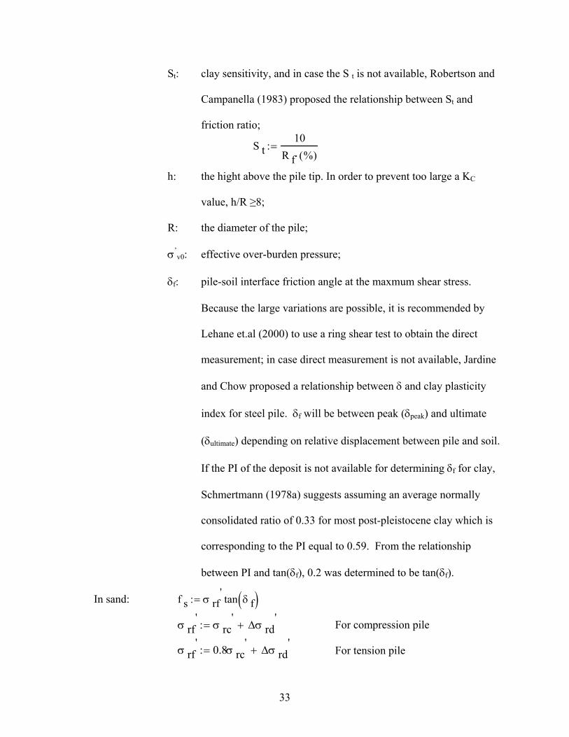
St: clay sensitivity, and in case the S t is not available, Robertson and
Campanella (1983) proposed the relationship between St and
friction ratio;
S t10
R f %( )⋅:=
h: the hight above the pile tip. In order to prevent too large a KC
value, h/R ≥8;
R: the diameter of the pile;
σ’v0: effective over-burden pressure;
δf: pile-soil interface friction angle at the maxmum shear stress.
Because the large variations are possible, it is recommended by
Lehane et.al (2000) to use a ring shear test to obtain the direct
measurement; in case direct measurement is not available, Jardine
and Chow proposed a relationship between δ and clay plasticity
index for steel pile. δf will be between peak (δpeak) and ultimate
(δultimate) depending on relative displacement between pile and soil.
If the PI of the deposit is not available for determining δf for clay,
Schmertmann (1978a) suggests assuming an average normally
consolidated ratio of 0.33 for most post-pleistocene clay which is
corresponding to the PI equal to 0.59. From the relationship
between PI and tan(δf), 0.2 was determined to be tan(δf).
In sand:
For compression pile
f s σ rf'tan δ f( ):=
σ rf σ rc ∆σ rd+:=
For tension pile
' ' '
σ rf 0.8 rc ∆σ rd+:='
σ' '
33

σ rc'
0.029 q c⋅σ ν0
'
Pa
⎛⎜⎜⎝
⎞
⎠
0.13
⋅hR
⎛⎜⎝
⎞⎠
0.38−⋅:=
∆σ rd' 4G R cla⋅
R:=
G q c 0.0203 0.00125q c
Pa σ ν0'
⋅
⋅+ 1.216 10 6−⋅q c
2
Pa σ ν0'
⋅
⋅−⎛⎜⎜⎜⎝
⎞⎟
⎠
1−
⋅:=
where: σ'rf: radial effective stress at maximum shear stress;
σ'rc: radial effective stress on side after equalization;
∆σ'rd: the net dilatant component;
Pa: the atmosphere pressure;
G: the sand shear modulus;
Rcla: the pile’s center-line-average roughness. It is qual to 10-5 for steel
pile, 10-4 for very rough casing of concrete pile and 3*10-5 for
prestressed concrete pile;
δf: pile-soil interface friction angle at the maxmum shear stress. It is
recommended by Jardine and Chow (1996) to use an interface-
direct or a ring-shear test with the same roughness and hardness as
the pile material and same effective normal stress as the field; in
case direct measurement is not possible, Jardine and Chow
recommended to use the relationship between δcv (critical state
interface friction angle) and sand mean particle size (d50) for steel
pile and assume δf is equal to δcv. From correspondence with the
authors, it was found that they are currently conducting sets of
34

interface shear tests on sands sheared against concrete but have not
finished yet. For now, it is recommended to assume δf between
concrete pile and sand is not so different from δf between steel pile
and sand. Since D50 of Florida soil is somewhat between 0.1 mm
and 0.3 mm, it was decided to use 30° as δf.
Eslami and Fellenius Method
This method was proposed by Eslami and Fellenius from the study of 102 cases around the
world. This is the method that uses cone tip resistance (q c) and pore pressure (u) to predict the
axial pile capacity. CPT sleeve friction is only used to identify the soil type.
q t = q egThe pile’s unit tip capacity:
where: qeg is the geometric average of the effective cone resistance. The
effective cone resistance is calculated by subtracting the
hydrostatic pressure from the cone resistance if pore pressure data
is not available.
The influence zone proposed by the Eslami and Fellenius is as follows:
2D above and 4D below the pile tip when the pile is installed through a
dense soil into a weak soil.
8D above and 4D below the pile tip when the pile is installed through a
weak soil into a dense soil.
The pile’s unit skin friction: fs = cs * qewhere: CS is functions of soil type.
qe is average of the effective cone resistance within the calculation layer.
35

The effective cone resistance is calculated by subtracting the
hydrostatic pressure from the cone resistance if pore pressure data
is not available.
Powell et al. Method
This method was proposed by Powell et al. from the study of 63 steel driven or jacked
piles. The soil condition ranged from soft normal-consolidated clay to stiff over-consolidated
clay and two sand sites. The parameters used by this method are cone tip resistance (qc) and pore
pressure (u), undrained shear strength(su), and a soil profile to predict the axial pile capacity.
The pile’s unit skin friction:
k 1 10.5 13.3log
q c σ ν0−
σ ν0'
⎛⎜⎜⎝
⎞
⎠
⋅+:=f sq c σ ν0−
k 1:=
where: qc is CPT tip resistance, with pore pressure correction for piezocones,
σv0 is the total overburden stress,
σ’v0 is the effective overburden stress.
In order to calculate the effective overburden stress, hydrostatic pressure has been used. A
reduction in k1 needs to be applied if L/D >60. The reduction factor is recommended by both
Semple and Rigden (1948) and is included in the procedure suggested by Randolph and Murphy
(1985).
The pile’s unit tip capacity: k 2N kt
9:=q t
q c σ ν0−
k 2:=
where: Nkt is cone factor, range from 10 to 20 based on local experience. 15 was
used in current study.
36

UWA-05 Method
This method was proposed by Lehane et al. in 2005. This method is especially used to
predict pile ultimate capacity in sand.
q t q ca 0.15 0.45 1D int
2
D2−
⎛⎜⎜⎝
⎞
⎠⋅+
⎡⎢⎢⎣
⎤⎥⎥⎦
⋅:=The pile’s unit tip capacity:
where: qca is calculated by minimum path rule. Dint is the
internal diameter for pipe pile, D is the outer diameter of the pile.
The pile’s unit skin friction:
f s 0.03 q c⋅ 1D int
2
D2−
⎛⎜⎜⎝
⎞
⎠
0.3
⋅ maxhD
2,⎛⎜⎝
⎞⎠
⎛⎜⎝
⎞⎠
0.5−4 G⋅
∆rD
⋅+⎡⎢⎣
⎤⎥⎦
⋅ tan δ cv( )⋅:=
G q c 185⋅
q c
Pa
σ ' v0Pa
⎛⎜⎜⎜⎜⎝
⎞
⎟⎟
⎠
0.7−
⋅:=
where: qc: average CPT tip resistance within the calculated soil layer;
Pa: the atmosphere pressure;
G: the sand shear modulus;
h: the hight above the pile tip. In order to prevent too large a KC
value, h/R ≥8;
σ’v0: effective over-burden pressure;
∆r: interface dilation, 0.02 mm was used by current study;
δcv: constant volume interface friction angle between sand and pile.
37

Since the large variations are possible, it is recommended to use ring shear test to obtain
the direct measurement; In the absance of lab tests, The trends between δcv and D50
recommended by ICP-05 with the upper limit 0.55 for the tan(δcv) are considered reasonable.
Since D50 of Florida soil is somewhat between 0.1 mm and 0.3 mm, it was decided to use 29° as
δcv, which will give the tan(δcv) 0.55.
Zhou et al. Method
This method was proposed by Zhou et al. after the study of 96 pre-cast driven concrete
piles in several eastern Chinese provinces. It provides a satisfactory predictions (80% of the
predicted errors are within 20% of the true load test results). The soil condition ranged from
sand to clayey soil. The parameters used by this method are cone tip resistance (qc) and sleeve
friction (fs) to predict the axial pile capacity. One of the interesting points about this method is
that it predicts limit load capacity in stead of ultimate load capacity. The limit load is defined as
the load near the starting point of the straight line portion on the load test curve, the point where
the shaft resistance of pile would be fully mobilized, while the end resistance only partially
mobilized. If the point is not obvious form the data, they recommend using the load at a relative
settlement of 0.4 – 0.5.
The pile’s unit tip capacity:
where: qca is average CPT tip resistance within 4D above and 4D below the pile q t α q ca⋅:=
tip;
α is the function of soil type and qca , use the following equations to
calculate α value;
α 0.71 q ca0.25−
⋅:=
α 1.07 q ca0.35−
⋅:=
Soil Type I:
Soil Type II:
38

Soil type is defined as: Soil Type I: qca > 2 MPa and fsa / qca < 0.014
Soil Type II: other than Soil Type I.
The pile’s unit skin friction: f :=s β f sa⋅
where: fsa is average CPT sleeve friction along the calculated soil layer;
β is the function of soil type and fsa , use the following equations to
calculate β value.
β 0.23 f sa0.45−
⋅:= Soil Type I:
β 0.22 f sa0.55−
⋅:= Soil Type II:
39

Figure 2-1. Regular cone penetrometer
40

CHAPTER 3 MATERIALS AND METHODS
Dual Tip Penetrometer (DTP)
The DTP is the latest version of a series of devices developed at the University of Florida
intended for identifying cemented sands. Daniel Hart developed the first version of the device in
1996 while he was a graduate student at the University of Florida. The device at that time had a
lip welded onto the top of the friction sleeve. However, this meant that the bearing reading
measured by the lip was added to the frictional component measured by the friction sleeve strain
gauge. The lip also made it difficult to remove the cone from the ground. In 1998, Randell
Hand eliminated the welded lip and welded a bearing annulus onto the friction reducer coupler.
The annulus was therefore located about 20 inches above the top of the cone’s friction sleeve.
Strain gages were used to measure resistance in the annulus. The voltage output was translated
into a second “qc” (tip resistance) reading. Steve Kiser and Hogentogler & Co. Inc. improved on
this design and came up with the dual tip penetrometer in 1999. In 2004, Hogentogler & Co. Inc.
converted the DTP from analog into digital cone, which is the latest version of DTP equipped in
the cone truck at the State Material Office.
The DTP is similar to conventional cone penetrometers except for a second tip (actually an
annulus) just above the friction sleeve as shown in Figure 3-1. The second tip has the same
angle (60°) and bearing area (10 cm2) as the regular cone. The first tip was originally designed to
break down the cohesive bonds of cemented sand while the second tip was meant to measure the
residual or broken-up bearing resistance. Based on the relationship between Tip 1 and Tip 2
along with the soil profile, through a large number of experiments, cemented sand identifiers
would be identified.
41

Locate Cemented Sites
Cemented sands exist in many areas of the United States, including California, Texas,
Florida, and along the banks of the lower Mississippi River. Lightly cemented sands are usually
misidentified in the CPT test, which can cause design problems. SPT borings log are one
resource used to identify cemented sand. However, if the cementation is very weak and can be
easily broken by finger pressure, it might not be noticed by the field technicians.
In order to incorporate cemented sands into the new proposed design method, strongly
cemented and lightly cemented sand sites were identified using two databases, FDOT and UF.
There are hundreds of in-situ and load test data in these two databases. Both SPT data and
boring logs were searched to identify cemented sand sites. CPT data were also searched and
combining with SPT N (Qc/N) to locate cemented sand sites. All previous projects reports were
reviewed to find soil and load test data. In case of sites where load test and SPT data were
available, but no CPT data, the sites were flagged for future CPT and DTP testing.
There were a total of 21 cases where load test, SPT and CPT (DTP in some cases) are all
available. Figure 3-2 shows the relative locations of these 21. These cases were used to
calibrate the ultimate pile capacity prediction methods and their corresponding LRFD resistance
factors Φ.
Axial Ultimate Pile Capacity Prediction Methods
A total of 14 prediction methods have been analyzed in my research. They are: the
Schmertmann method, de Ruiter and Beringen method, Penpile method, Price and Wardle
method, Tumay and Fakhroo method, Aoki and De Alencar method, Philipponnat method,
LCPC (Bustamante and Gianeselli) method, Almeida et al. method, MTD (Jardine and Chow)
method, Eslami and Fellenius method, Powell et al. method, UWA-05 method, and Zhou et al.
method. Because most of the methods involve complicated calculation and digital CPT data
42

make these calculations time intensive, a MathCAD program was used to calculate each of
predictions. For each method there is one MathCAD program that was presented in the
appendix.
Figure 3-3 shows the program for the Philipponnat method. The colored fields are inputs.
The CPT data input is an Excel file formatted with four columns (depth, tip resistance, sleeve
friction, and pore pressure). Other inputs are diameter or edge length of pile, embedment length,
layer depths. After all required fields have been inputted, the program will calculate ultimate tip
resistance, ultimate skin friction and Davisson capacity (1/3 of ultimate tip resistance + ultimate
skin friction).
Load and Resistance Factor Design (LRFD)
Over the past two decades, Load and Resistance Factor Design (LRFD) have been
incorporated in structural and geotechnical designs. One of the benefits of LRFD is its consistent
reliability in design practice. Many state DOT’s, including FDOT, are now implementing
AASHTO (American Association of State Highway and Transportation Officials) LRFD
Specifications. Hence, the object of my research is to update FDOT’s pile/shaft design
procedure based on CPT and DPT data and access the LRFD resistance factor for each pile
capacity prediction method. Even though LRFD requires both load and resistance factors, the
resistance factor is considered as a variable for each static pile capacity prediction method
whereas load factors are typically constants, based on local experience.
Modified First Order Second Moment (FOSM) Approach
The LRFD approach used in my research is the modified FOSM (First Order Second
Moment Approach). The modification was developed at the University of Florida (Styler, 2006)
due to the difference between FORM (First Order Reliability method) and FOSM resistance
factor in NCHRP Report 507. The modified portion in FOSM is the term COV (Q). The
43

previous FORM assumes COV (Q) = COV (QD) + COV (QL). It was found that this equation
was incorrect and a modified COV (Q) was formulated as:
COV Q( )
Q D2
Q L2
λ QD2
⋅ COVQD2
⋅ λ QL2
COVQL2
⋅+
Q D2
Q L2
λ QD2
⋅ 2Q DQ L
⋅ λ QD⋅ λ QL⋅+ λ QL2
+
:=
where: QD/QL = Dead to live load ratio, varies from 1.0 to 3.0 (spans, L =
57-170 ft. Since it is not very sensitive, a value of 2.0 used
herein),
λQD, λQL = Dead load and live load bias factors, λQD = 1.08, λQL =
1.15 (recommended by AASHTO 1996/2000),
COVQD, COVQL = Dead load and live load coefficients of
variation,
COVQD = 0.128, COVQL = 0.18 (recommended by AASHTO).
Based on this modified FOSM, it was concluded that the difference between FORM and
FOSM was little if any. Since FORM involves complicated calculation process, the modified
FOSM is the approach used in my research.
The following section provides a detailed deviation of LRFD resistance factor using
modified FOSM approach.
Limit state equation
In this approach, load and resistance are assumed to be lognormal distribution. Therefore,
the limit state equation is as follows:
44

G ln R( ) ln Q( )−:=
E G( ) E ln R( )( ) E ln Q( )( )−:=
E ln R( )( ) ln E R( )( )12
ln 1 COV R( )( )2+⎡⎣ ⎤⎦⋅−:=
E ln Q( )( ) ln E Q( )( )12
ln 1 COV Q( )( )2+⎡⎣ ⎤⎦⋅−:=
E G( ) lnE R( ) 1 COV Q( )( )2
+⋅
E Q( ) 1 COV R( )( )2+⋅
⎡⎢⎢⎣
⎤⎥⎥⎦
:=
It is assumed that R and Q are statistically independent, therefore σG:
σ G VAR ln R( )( ) VAR ln Q( )( )+:=
σ G ln 1 COV R( )( )2+⎡⎣ ⎤⎦ 1 COV Q( )( )2
+⎡⎣ ⎤⎦⋅⎡⎣ ⎤⎦:=
where: COV(R), COV(Q) = Resistance, load coefficient of variation.
Reliability index β
E G( )σ G
:=
β
lnE R( ) 1 COV Q( )( )2
+⋅
E Q( ) 1 COV R( )( )2+⋅
⎡⎢⎢⎣
⎤⎥⎥⎦
ln 1 COV R( )( )2+⎡⎣ ⎤⎦ 1 COV Q( )( )2
+⎡⎣ ⎤⎦⋅⎡⎣ ⎤⎦:=
E R( )E Q( ) exp β ln 1 COV R( )( )2
+⎡⎣ ⎤⎦ 1 COV Q( )( )2+⎡⎣ ⎤⎦⋅⎡⎣ ⎤⎦⋅⎡⎣ ⎤⎦⋅
1 COV Q( )( )2+
1 COV R( )( )2+
:=
Resistance factor Φ
The LRFD equation:
φ Rn ≥ Σ η γ i Q i
45

where: Φ = Resistance factor
Rn = Nominal Resistance
η = Load modifier for importance, redundancy and ductility
γi = Load factors
Qi = Force effects
Load modifier η is set equal to 1 which leaves all uncertainty on the resistance factor φ.
For driven pile design, two load effects, dead load QD and live load DL are considered.
Therefore, γD and γL are considered as load factors for dead load and live load, respectively. The
LRFD equation becomes:
φ Rn ≥ γD QD + γL QL
φγ D Q D⋅ γ L Q L⋅+
R n≥
E R( ) λ R R n⋅:=Since:
where: λ R = Mean bias (mean of resistance bias factor);
λ R1
N
i
λ Ri∑=
N:=
λ Ri
R miR ni
:=
where: R mi = Measured capacity from load test data
R ni = Predicted capacity form CPT data
N = The number of cases
φγ D Q D⋅ γ L Q L⋅+
E R( )
λ R
≥
46

By inserting E(R) into the above equation, the follow equation can be derived:
φ
λ R γ D Q D⋅ γ L Q L⋅+( )⋅1 COV Q( )( )2+
1 COV R( )( )2+
⋅
E Q( ) exp β ln 1 COV R( )( )2+⎡⎣ ⎤⎦ 1 COV Q( )( )2
+⎡⎣ ⎤⎦⋅⎡⎣ ⎤⎦⋅⎡⎣ ⎤⎦⋅
≥
Since the dead load and live load are considered as statistically independent, E (Q) can be
expressed as follows: Q γ D Q D⋅ γ L Q L⋅+:=
E Q( ) λ QD Q D⋅ λ QL Q L⋅+:=
where: λ QD, λ QL = Dead load and live load bias factors;
λQD=1.08, λQL = 1.15 (recommended by AASHTO 1996/2000)
By inserting E(Q) into the equation for resistance factor, and divide both numerator and
denominator by QL, the follow equation results:
φ
λ R γ DQ DQ L
⋅ γ L+⎛⎜⎝
⎞
⎠⋅
1 COV Q( )( )2+
1 COV R( )( )2+
⋅
λ QDQ DQ L
⋅ λ QL+⎛⎜⎝
⎞
⎠exp β ln 1 COV R( )( )2
+⎡⎣ ⎤⎦ 1 COV Q( )( )2+⎡⎣ ⎤⎦⋅⎡⎣ ⎤⎦⋅⎡⎣ ⎤⎦⋅
≥
This equation was traditionally used to calibrate the resistance factor using FOSM in
AASHTO’s specifications by assuming COV (Q) 2 = COV (QD) 2 + COV (QL) 2. However, as
mentioned previously, this assumption is incorrect. The correct derivation is as follows:
VAR Q( ) Q D2 VAR γ D( )⋅ Q L
2 VAR γ L( )⋅+:=
QD γ D Q D⋅:=
QL γ L Q L⋅:=
47

COV QD( ) 2 VAR γ D( ) Q D2⋅
λ QD2
Q D2
⋅
:=
COV QL( ) 2 VAR γ L( ) Q L2
⋅
λ QL2
Q L2
⋅
:=
VAR γ L( ) λ QL2
COV QL( ) 2⋅:=
VAR γ D( ) λ QD2
COV QD( ) 2⋅:=
COV Q( )2 VAR Q( )
E Q( )2:=
VAR Q( ) Q D2
λ QD2
⋅ COV QD( )2⋅ Q L
2λ QL
2⋅ COV QL( )2
⋅+:=
COV Q( )2
Q D2
Q L2
λ QD2
⋅ COV QD( )2⋅ λ QL
2COV QL( )2
⋅+
Q D2
Q L2
λ QD2
⋅ 2Q DQ L
⋅ λ QD⋅ λ QL⋅+ λ QL2
+
:=
By inserting COV(Q) into the resistance equation, the following equation can be obtained:
φ
λ R γ DQ DQ L
⋅ γ L+⎛⎜⎝
⎞
⎠⋅
1
Q D2
Q L2
λ QD2
⋅ COV QD( )2⋅ λ QL
2COV QL( )2
⋅+
Q D2
Q L2
λ QD2
⋅ 2Q DQ L
⋅ λ QD⋅ λ QL⋅+ λ QL2
+
+
1 COV R( )( )2+
⋅
λ QDQ DQ L
⋅ λ QL+⎛⎜⎝
⎞
⎠exp β ln 1 COV R( )( )2
+⎡⎣ ⎤⎦ 1
Q D2
Q L2
λ QD2
⋅ COV QD( )2⋅ λ QL
2COV QL( )2
⋅+
Q D2
Q L2
λ QD2
⋅ 2Q DQ L
⋅ λ QD⋅ λ QL⋅+ λ QL2
+
+
⎛⎜⎜⎜⎜⎜⎜⎜⎝
⎞⎟⎟⎟⎟⎟⎠
⋅
⎡⎢⎢⎢⎢⎢⎢⎢⎣
⎤⎥⎥⎥⎥⎥⎥⎥⎦
⋅
⎡⎢⎢⎢⎢⎢⎢⎢⎣
⎤⎥⎥⎥⎥⎥⎥⎥⎦
⋅
≥
48

where: γD = Dead load factor (1.25, recommended by AASHTO (1996/20001)),
γL = Live load factor (1.75, recommended by AASHTO 1996/2000),
QD/QL = Dead to live load ratio, varies from 1.0 to 3.0 (spans, L = 57-170 ft,
is not very sensitive, a value of 2.0 used herein)
λR = Mean of resistance bias factor,
COV (R) = Resistance coefficient of variation ,
λQD, λQL = Dead load and live load bias factors,
λQD = 1.08, λQL = 1.15 (recommended by AASHTO 1996/2000),
COVQD, COVQL = Dead load and live load coefficients of variation,
COVQD = 0.128, COVQL = 0.18 (recommended by AASHTO)
βT = Target reliability index, AASHTO and FHWA recommend values from
2.0 to 3.
Of major importance in estimating LRFD resistance factor, Φ, are the resistance’s bias
factor (λR), and the resistance’s coefficient of variation (COV(R)). Both are computed from: 1)
the nominal predicted resistance, Rni (predicted pile capacity), and 2) the measured pile capacity,
Rmi, i.e. load test results. Based on the ratio of measured to predicted pile capacities, λRi, for
each of the sites, the mean, λR, standard deviation, σR, and coefficient of variation, COV(R),
were determined for all 14 CPT methods. Using these inputs, the LRFD resistance factors, Φ,
were determined with a reliability index, β of 2.5 for each method. Because driven piles are
usually in groups and redundancy will require lower reliability, 2.5 was used in my research.
Differentiate Ultimate Skin Friction and Tip Resistance from Load Test Data
All of the load tests were conventional top-down static load tests performed for which
load-settlement data exist (see Figure 3-4.). Using FDOT’s load testing protocol (i.e.
49

Specification Section 455), the Davisson Capacity was assessed for each load versus settlement
curve. The Davisson Capacity, referred to as the measured capacity, Rm, generally occurs for
settlements that are tolerable (i.e. less than 1”), under service loading conditions. These values
were subsequently used with the predicted capacities, Rn, (where Rn = QS ult + 1/3 * QT ult) to
assess the LRFD resistance factor, Φ for each of the fourteen CPT methods.
However, the load versus settlement curve does not provide the ultimate skin friction and
tip resistance. In order to evaluate the accuracy of each prediction method for ultimate skin
friction and tip resistance separately, each needs to be estimated using this load test curve.
Figure 3-5 shows the proposed process that was developed to separate the two attributes. For the
majority of the tests, the piles were not loaded sufficiently to induce a plunging failure. While
the ultimate skin friction is likely fully mobilized at small displacements (0.1”), the tip resistance
is not. Thus, it is not possible to determine the ultimate tip resistance (i.e., the tests ended after
one inch displacement was reached, whereas two inches of displacement or approximately D/10
[D is in inches] is typically needed to induce a plunging failure) unless the load test curve is
extrapolated to the two inch value. The idea of extending the load test curve follows from
deBeer’s method for determining pile capacity.
The proposed differentiate method is as follows (see Figure 3-5 for an example of the
process):
a. The load test is plotted in log-log space. b. Two straight trend lines are drawn among the data points, with the second line
extended or extrapolated to two inches. c. Two distinct loads are indentified: the first occurs at the intersection of the two
sloped lines and the other at the presumed displacement of two inches. d. Since the first load typically occurred at a displacement of approximately 0.1 to
0.2 inches, (i.e., 5% to 10% of the extrapolated value), it was assumed that 5% of
50

the ultimate tip resistance was mobilized. Therefore, the first load is assumed to be the sum of the ultimate skin friction and 5% of the tip resistance, while the second load is the ultimate skin plus tip resistance. Therefore, the separate contributions of ultimate tip and skin friction can be calculated.
The Proposed UF Method
The proposed method uses the following equation to estimate the ultimate pile unit tip
resistance, qt, from the CPT tip resistance, qc:
qt = kb * qca (tip) ≤ 150 tsf
where: kb is a factor that depends on the soil type as shown in Table 3-1.
The soil type was determined using the soil classification chart for the
standard electronic friction cone (Robertson et al, 1986) which
includes tip resistance and sleeve friction. Soil cementation was
determined by SPT samples, DTP tip2/tip1 ratio or SPT qc/N ratio
(>10).
qca (tip): the average CPT tip resistance, which is calculated as follows:
qca (tip) = (qca above + qca below ) / 2
qca above : average q c measured from the tip to 8 D above the tip;
qca below : average q c measured from the tip to 3 D below the tip for sand
or 1D below the tip for clay;
Impose the condition: qca above ≤ qca below, which means if qca above ≥ qca below,
let qca (tip) be equal to q ca below.
The proposed method uses the following equation to estimate the ultimate skin friction
resistance of the pile, fs, from the CPT tip resistance, qc:
fs = qca (side) *1.25 / Fs ≤ 1.27 tsf
51

where: Fs: friction factor that depends on the soil type as shown in Table 3-2.
The following criterion was used to determine the sand state based
on relative density: loose sand (R.D. < 40 %), medium dense sand
(40 % < R.D. < 70 %), and dense sand (R.D. >70 %).
qca (side) : the average qc within the calculating soil layers along the pile.
52

Table 3-1. Ultimate unit tip resistance factor k bWell Cemented Sand
Lightly Cemented Sand
Gravel Sand Slit Clay
0.1 0.15 0.35 0.4 0.45 1
Table 3-2. Ultimate unit skin friction empirical factor, Fs
Well Cemented Sand
Lightly Cemented Sand
Gravel and Dense Sand
Medium Dense Sand
Loose Sand
Silt, Sandy Clay, Clayey Sand
Clay
300 250 200 150 100 60 50
53

54
Figure 3-1. Dual tip penetrometer

55
Figure 3-2. The locations of 21 sites with load test data and CPT data

Figure 3-3. MathCAD program for Philipponnat method
56

Apalachicola River Bridge - Pier 3
0
100
200
300
400
500
600
0 0.2 0.4 0.6 0.8 1 1.2 1.4
Displacement (inches)
Load
(ton
s)
479 tons
Figure 3-4. Static load test, Apalachicola Bay Bridge (pier 3)
57

Jacksonville Industrial Zone 1
10
100
1000
0.01 0.1 1 10Displacement (inches)
Load
(tons
)
352.5 tons249 tons
Example: S + 5 % T = 249 tons S + T = 352.5 tons S = 243.5 tons T = 109 tons S : Ultimate Skin Friction T : Ultimate Tip Resistance
Figure 3-5. Separate the ultimate skin friction and tip resistance
58

CHAPTER 4 RESULTS
This chapter includes two parts. The first provides a synopsis of the DPT and CPT results
from various sites and the discussion of the cemented sand identifier. The second part is the
evaluation of current axial ultimate pile capacity prediction methodologies using LRFD
statistical method and the proposed method, including its verifications.
Identification of Cemented Sand
Cemented sands exist in many areas of the United States, including California, Texas,
Florida, and along the banks of the lower Mississippi River. They also exist in Norway,
Australia, Canada, and Italy (Puppala et al. 1995). If the sands found with a CPT test are not
known to be cemented, the high bearing readings may be misinterpreted as being due to high
relative densities. This can lead to an underestimation of the liquefaction potential of the soil
and overestimate the ultimate pile capacity. It is a very challenging soil type for geotechnical
engineers. It is therefore important to identify such soil before the design of foundation. In
previous practice, engineers used SPT borings and CPT (Qc/N) to identify cemented sand.
However, there are two drawbacks: firstly, lightly cemented sand may not be able to be
identified by field technicians since the strength between sand particles is very weak, and
secondly, the SPT provides a discontinuous data so that engineer judgment is required to
estimate the N value between data points for calculating Qc / N ratio. It would be very beneficial
if the DTP could be used to identify cemented sand.
DTP & CPT Test Data at FDOT Bridge Sites
Many FDOT’s bridge sites have been revisited and had DTP and CPT tests performed.
DTP and CPT tests were usually performed in pairs for comparison. All field tests were
conducted by personnel from the State Material Office (SMO). The sites were chosen so that
59

load tests and SPT data were available, and several sites also had cemented sand presented. The
sites include: Archer Landfill (Archer, FL), I-95 at Edgewood Avenue (Jacksonville, FL),
Apalachicola River Bridge, Pier 3 (Apalachicola, FL), West Bay Bridge, Pier 20 (Bay County,
FL), Port Orange Relief Bridge (Port Orange, FL), University of Central Florida (Orlando, FL),
I-295 at Blanding Blvd (Jacksonville, FL), I-295 at Normandy Blvd. (Jacksonville, FL), and
White City Bridge, Pier 5 and Pier 8 (White City, FL).
Archer Landfill Site
This site is one of the first sites used for DTP testing. The Archer landfill is an excellent
site for initial scrutiny. Located in Archer, Florida, this site contains a very clean, fine sand
deposit peripheral to the outside of the clay liner boundary. This area has been used for many
years as a borrow area, where clean sands were mined for daily cover of the landfill debris.
No SPT data is available for this site. Figure 4-1 shows the CPT tip resistance, DTP Tip 1
and Tip 2 resistances. The Tip 1 and CPT tip resistance are very close to each other. Therefore,
the second tip (the one above the friction sleeve) does not influence the reading of the first tip
(the one at the same location as the CPT). This phenomenon was found in all paired CPT and
DTP tests, which means the distance between these two tips is sufficient enough to eliminate the
interaction between each other. Another finding is that the relative magnitudes between DTP
Tip 2 reading (T2) and Tip 1 reading (T1) for the clear fine sand equal 0.5.
Figure 4-2 shows the comparison between friction ratios of CPT and DTP. From the plot,
it can be found that the friction ratio of the DTP is much higher than that of CPT for sand (~ 3
times). The main reason for this increase is the normal stress adjacent to the friction sleeve due
to the second tip. Therefore, the shear stress near the friction sleeve is also increased. The
discrepancy in friction ratios between the DTP and CPT does not allow for soil classification
unless a new soil classification chart for the DTP is created. However, the main purpose of DTP
60

is to identify cemented sand using cemented sand identifiers (T2/T1 ratio). This ratio is
presented below in the following analysis.
I-95 at Edgewood Avenue Site
This site is located in Jacksonville and is a FDOT bridge site. Figure 4-3 shows the CPT
tip resistance, DTP Tip 1 and Tip 2 resistances. The Tip 1 and CPT tip resistance are very close
to each other. It can be found that the T2/T1 ratio varies with depth. Since the depth is function
of soil type, T2/T1 is a function of soil type, depth, or both. Through later test results, it was
found that the T2/T1 ratio is solely a function of soil type.
Figure 4-4 shows the comparison between the friction ratios of the CPT and DTP. From
the plot, it can be observed that the DTP’s is again higher than the CPT’s for sandy soil (about 3
times), but it is close to the CPT’s for clayey soil. Since the friction ratio of DTP is different
from that of CPT and hence could not be used to classify the soil, the friction ratio of following
cases will not be presented.
Figure 4-5 shows the comparison between the T2/T1 ratio and Qc/N ratio with depth.
Generally speaking, when the Qc/N ratio is less than 3, the soil is considered as a clayey, silty
soil. With Qc/N ratios between 3 to 10, the soil is considered a regular sand, and above 10,
cemented sand may be encountered. For the I-95 at Edgewood site, the soil profile is as follows:
loose to medium dense sand with a thin layer of silt (0 feet – 27 feet), clay (27 feet – 36 feet),
and dense, silty fine sand (36feet – 59feet). This was confirmed by the Qc/N ratio. The T2/T1
ratio is 0.5 for loose to medium dense sand, greater than or equal to 1 for clayey silty soil, and
greater than 1 for very dense, silty sand.
Apalachicola River Bridge Site
This site is also a FDOT bridge site located in Apalachicola, FL. Figure 4-6 shows the
CPT tip resistance, DTP Tip 1 and Tip 2 resistances. The Tip 1 and CPT tip resistance are very
61

close to each other. The soil profile in this site is as follows: two lightly cemented sand layers (0
feet – 25 feet), sandy silt (25 feet – 45 feet), silty clay (45 feet – 60 feet), and lightly cemented
sand layer (under 60 feet). Figure 4-7 gives the comparison between the T2/T1 ratio and Qc/N
ratio with depth at the Apalachicola River Bridge site. The T2/T1 ratio is less than 0.5 for lightly
cemented sand, between 0.5 to 1 for sandy silt and silty clay soil.
West Bay Bridge Site
This site is a FDOT bridge site located in Bay County, FL. Figure 4-8 shows two CPT tip
resistances, DTP Tip 1 and Tip 2 resistances. The reason for presenting two CPTs is to show
that there is significant spatial variability at this site. These two CPTs are within 100 feet and are
totally different. The DPT Tip 1 and CPT1 Tip resistances are very close under 68 feet but DTP
T1 is much higher than CPT1 tip resistance above 68 feet. However, DTP T1 is very similar to
the CPT2 tip resistance at the depth above 64 feet but significant smaller at the depth below 64
feet. In this site, there are two lightly cemented sand layers and one well cemented sand layer.
Figure 4-9 provides a comparison between T2/T1 ratio and Qc/N ratio along the depth at this site.
The T2/T1 ratio is less than 0.5 for lightly cemented sand, and close to 1 for well cemented sand.
Port Orange Relief Bridge
This site is a FDOT bridge site located in Port Orange, FL. Figure 4-10 shows CPT tip
resistance, DTP Tip 1 and Tip 2 resistances. The DPT Tip 1 and CPT1 Tip resistances are very
close to one another. At this site, there are two well cemented sand layers with one clayey silt
and one lightly cemented sand layer in the middle.
Figure 4-11 shows a comparison between T2/T1 and Qc/N with depth. The T2/T1 ratio is
less than 0.5 for lightly cemented sand and clayey silt and close to 1 for well cemented sand.
The interesting finding in this figure is that the Qc/N ratio is higher for lightly cemented sand
than that for well cemented sand. The lightly cemented sand is loose to medium dense sand with
62

very low N blow count; therefore, it does not require a high tip resistance (qc) to acquire very
large Qc/N ratio. Therefore, this ratio cannot indicate just how strong the cementation is.
University of Central Florida
This site is located at the University of Central Florida, Orlando, FL. Figure 4-12 shows
CPT tip resistance, DTP Tip 1 and Tip 2 resistances. The DPT Tip 1 and CPT1 Tip resistances
are similar. At this site, there are two lightly cemented sand layers (T2/T1 <0.5) and four well
cemented sand layers (T2/T1 ≈ 1) with one clayey silt layer with shell (38 feet – 53 feet) and
two clay layers (4 feet – 6 feet, 30 feet – 34 feet).
Figure 4-13 gives a comparison between T2/T1 and Qc/N with depth. The T2/T1 ratio is
less than 0.5 for lightly cemented sand, close to 1 for well cemented sand, and less than 0.5 for
clay and clayey silt. The interesting finding at this site is that the T2 values in clay and clayey
silt are very low and even negative. That means that the clay is highly sensitive and loses its
shear strength dramatically after the disturbance of the first tip.
I-295 at Blanding Blvd Site
This is a site in Jacksonville, FL. Figure 4-14 shows CPT tip resistance, DTP Tip 1 and
Tip 2 resistances. At this site, there are two sand layers (0 feet – 32 feet, 53 feet – 58 feet) with
four lightly cemented sand layers within (T2/T1 <0.5) and one clayey silt layer (32 feet – 53 feet)
with one lightly cemented sand within. Figure 4-15 shows the comparison between T2/T1 and
Qc/N with depth. The T2/T1 ratio is less than 0.5 for lightly cemented sand, close to or greater
than 1 for clayey silt.
I-295 at Normandy Blvd. Site
This is another site in Jacksonville, FL. Figure 4-16 shows CPT tip resistance and DTP
Tip 1 and Tip 2 resistances. At this site, there are three lightly cemented sand layers (T2/T1
63

<0.5). Figure 4-17 shows a comparison between T2/T1 and Qc/N with depth. The T2/T1 ratio is
less than 0.5 for lightly cemented sand.
White City Bridge Site (Pier 5)
This is a site in White City, FL. Figure 4-18 shows CPT tip resistance and DTP Tip 1 and
Tip 2 resistances. At this site, there are three lightly cemented sand layers, two silty sand layers
and three clay layers. Figure 4-19 indicates the comparison between T2/T1 and Qc/N with depth.
The T2/T1 ratio is less than 0.5 for lightly cemented sand, is between 0.5 – 1 for silty sand and
close to or greater than 1 for clay.
White City Bridge Site (Pier 8)
This is the second pier at White City Bridge site in White City, FL. Figure 4-20 shows
CPT tip and DTP Tip 1 and Tip 2 resistances. There are three lightly cemented sand layers, one
silty sand layer, one clay layer, and one sand layer. Figure 4-21 gives the comparison between
T2/T1 and Qc/N with depth. The T2/T1 ratio is less than 0.5 for lightly cemented sand, is
between 0.5 and 1 for silty sand, greater than 1 for clay and 0.5 for sand.
Identifier for Cemented Sand Summarized from DTP Data
Based on the data collected to date, the T2 /T1 ratio appears to be a reasonable predictor or
identifier for cemented sand. The following ranges for each soil type are based on the limited
data collected in Florida. It may be different elsewhere and more data needs to be collected to
verify these values.
T2/T1:
≈ 0.5 Non-Cemented Sand (Loose and Medium Dense Sand)
= 0.3~0.5 Lightly Cemented Sand
≈ 1 Strongly Cemented Sand
= 0.5~1 Silty Sand, Sandy Silt and Silty Clay
64
< 0.5 Highly Sensitive Clay
> 1 Dense Silty Sand
≥1 Clayey Silt, Silty Clay and Clay
The reasons for the identifier having different values for different soil types may seem
ambiguous. However, the following is one possible explanation that will have to be verified by
additional testing.
For non-cemented sand (loose and medium dense sand), T2 is less than T1 due to the
compression of the sand after the first tip penetrates the soil. The value 0.5 for the identifier is
function of the location of the second tip. Therefore, it is the unique character for the DTP used
in my research. However, for dense sand, due to the dilation of sand particles after the
disturbance of the first tip, T2 is greater than T1. For highly sensitive clay, the disturbance of the
first tip dramatically reduces the shear strength of clay that results in the T2/T1 of less than 0.5.
For lightly cemented sand, the cementation bonds are totally broken after penetration of the first
tip so that T2 is the same as that for non-cemented sand. However, T1 for lightly cemented sand
is higher than that for non-cemented sand, which causes T2/T1 ratio to be less than 0.5. For well
cemented sand, the cementation bonds are so strong that they cannot all be broken or are only
partially destroyed. Therefore, T2 is close to T1 for well-cemented sand. For low sensitive clay,
clayey silt and silty clay, the penetration of the first tip may reduce the shear strength of the soil
and the reduction depends on the strength of clay. However, the excess pore pressure generated
by the intrusion of the first tip also increases T2. The resultant effects cause T2/T1 ratio to be
less than, close to or greater than 1. For a mixed soil such as silty sand and sandy silt, T2/T1 is
between 0.5 and 1 due to the combining effects.
65

Assessing LRFD Resistance Factors, Φ, Based on Reliability (Risk)
Two set of data were used for the LRFD assessment. They include 21 Florida cases and 28
in Louisiana. The data for Florida and Louisiana are analyzed separately to see how each
method works for their respective soil type (Florida: predominantly sand, Louisiana:
predominantly clay).
Criteria Used to Quantify Pile Capacity from Load Test Data
The criteria used to quantify pile capacity from load test data are the same as provided in
FDOT specification for 21 cases in Florida. It is defined as the load that causes a pile tip
deflection equal to the calculated elastic compression plus 0.15 inches plus 1/120 of the pile
width in inches for piles 24 inches or less in width. For piles greater than 24 inches, it is equal to
the calculated elastic compression plus 1/30 of the pile width (FDOT Specification 2007, 455-
2.2.1). The criteria are similar to Davisson capacity except for piles greater than 24 inches. All
methods predict the ultimate pile tip and skin capacity, therefore the nominal capacities are
calculated by the sum of ultimate skin capacity and 1/3 of ultimate tip capacity (Rn = QS ult + 1/3
* QT ult). The ratio of measure capacity (FDOT failure load) to the nominal capacity is used to
assess LRFD resistance factor.
Since clay is the predominant soil type in Louisiana, a typical load test curve is shown in
Figure 4-22. The ultimate pile capacity is less than the peak load. Therefore, it is not
appropriate to compare the predicted nominal capacities (Rn = QS ult + 1/3 * QT ult) with Davisson
capacity (QDavisson). Thus it was decided to compare the predicted ultimate pile capacity (Rult =
QS ult + QT ult) with the ultimate capacity from the load test (load at 2 inches of displacement).
According to FDOT specification, the allowable load of any pile tested must be either 50 % of
the maximum applied load or 50 % of the failure load, whichever is smaller.
66

LRFD Resistance Factor, Φ, for Florida Soil
Using the 14 CPT methods with the cone data from the 21 load test sites in Florida, - see
Tables 4-1, 4-2, and 4-3 - the ultimate skin friction, ultimate tip resistance, and Davisson
capacity were determined for each test pile. Also shown in these tables are the measured
ultimate skin friction, ultimate tip resistance, Davisson Capacity (from load test curve and the
proposed process to separate skin and tip). The highlighted cases represent cemented sand sites.
Shown in Figure 4-23 is a plot of the ratio (measured Davisson capacity/predicted Davisson
capacity) for each method for all 21 piles. In this plot, the cases are sorted by diameter. No
correction between the ratio λ and diameter. It was attemped to sort the case by length and there
still was no correction between the ratio and length. The methods above the value of one are
conservative. Next, the LRFD resistance factors, Φ, were assessed for each method.
Based on the ratio of measured to predicted pile capacities, λRi, for each of the sites, the
mean, λR, standard deviation, σR, and coefficient of variation, COVR, were determined for all 14
CPT methods. Using the computed mean, λR and coefficient of variation, COVR, the LRFD
resistance factors, Φ, were determined with a reliability index, β of 2.5 (recommended for
redundant foundation elements) for each method. Tables 4-4, 4-5, and 4-6 are the LRFD
resistance factors for ultimate skin friction, ultimate tip resistance, and Davisson capacity. The
last method is the one proposed by UF and was created by modifying the most promising method,
the Philipponnat method (1980).
Evident from Tables 4-4, 4-5, and 4-6, many of the methods result in higher resistance
factors, Φ. However, if the method has a substantial amount of scatter (a high COVR), Table 4-4
(e.g. Schmertmann, Prince, etc.), then the LRFD resistance factor, Φ, will be adjusted downward.
67

Of strong interest is a ranking of the 14 CPT methods investigated. The latter may be
determined as follows:
Rdesign = Φ Rn (i.e. predicted capacity from individual method)
However λR = Rm (i.e. Davisson) / Rn (predicted capacity)
Substituting the above equation into the Rdesign equation for Rn
Rdesign = (Φ/λR ) Rm
The term (Φ/λR) in the above equation identifies the percent of measured Davisson
capacity that is available for design. Obviously, the higher the (Φ/λR) term, the better the
method. Shown in Tables 4-4, 4-5, and 4-6 are (Φ/λR) terms for each method. Clearly,
Philipponnat & LCPC are the better methods. Interestingly, both the Philipponnat & LCPC
methods use just the CPT tip resistance, qc, to predict axial pile capacity. Finally, the proposed
UF method gives the value of 0.617 for Φ/λR, which means 61.7% of load test measured capacity
can be used for design.
LRFD Resistance Factor, Φ, for Louisiana Soil
Tables 4-7, 4-8, and 4-9 show the ultimate skin friction, ultimate tip resistance, and
ultimate pile capacity using the 14 CPT methods with cone data from 28 load test sites in
Louisiana. Shown in Figure 4-24 is a plot of the ratio (measured ultimate capacity/predicted
ultimate capacity) for each method. Again, methods above one are conservative. Tables 4-10, 4-
11, and 4-12 show the LRFD resistance factors for ultimate skin friction, ultimate tip resistance,
and ultimate pile capacity.
Shown in Tables 4-10, 4-11, and 4-12 are the (Φ/λR) terms for each method. From each
table, it is found that the ranking of prediction methods are different from the Florida data. The
68

Jardine & Chow (MTD) & Philipponnat methods are the better methods. However, both the
Jardine & Chow (MTD) and Philipponnat methods use only the CPT tip resistance, qc, to predict
axial pile capacity. The proposed UF method provides a value of 0.673 for Φ/λR, which is
second best method, and only slightly less than the MTD method.
In summation, it appears that the proposed UF method works very well for both sands
(Florida soil) and clays (Louisiana soil).
Evaluate the Prediction Methods Using the Bootstrap Method
After calculating the λi (Measured/Predicted) for each method and performing an LRFD
resistance factor analysis, one question remains: how representative is the data to the
population? Is there sufficient data to predict the pile capacity with a certain level of
confidence? Fortunately, a very powerful tool is available, termed the Bootstrap method.
This method estimates the sampling distribution of an estimator by resampling with
replacements from the original sample. For instance, there are total of 21 cases involving Florida
soil. We have 21 λs which are original samples from the whole population of λs. We want to
know how good the samples’ mean and standard deviations are.
There are three steps involved in the method. The first is to resample with replacement 21
λs from our original samples, which means picking λ one by one and after each pick it is placed
back into the pool for the next pick. Therefore, in this new set of samples, some λ's may appear
more than once, but some not at all. The second step is to calculate the mean and standard
deviation of the new sample set. The last step is to repeat the first and second steps numerous
times (at least 1,000). Finally, one obtains the distribution of the mean and standard deviation of
the new sample sets. From these one can determine how representative the samples are to the
population.
69
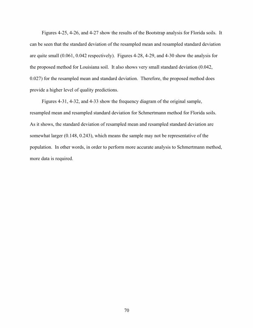
70
Figures 4-25, 4-26, and 4-27 show the results of the Bootstrap analysis for Florida soils. It
can be seen that the standard deviation of the resampled mean and resampled standard deviation
are quite small (0.061, 0.042 respectively). Figures 4-28, 4-29, and 4-30 show the analysis for
the proposed method for Louisiana soil. It also shows very small standard deviation (0.042,
0.027) for the resampled mean and standard deviation. Therefore, the proposed method does
provide a higher level of quality predictions.
Figures 4-31, 4-32, and 4-33 show the frequency diagram of the original sample,
resampled mean and resampled standard deviation for Schmertmann method for Florida soils.
As it shows, the standard deviation of resampled mean and resampled standard deviation are
somewhat larger (0.148, 0.243), which means the sample may not be representative of the
population. In other words, in order to perform more accurate analysis to Schmertmann method,
more data is required.

Table 4-1. Predicted ultimate skin friction for 14 CPT methods (Florida soil) Load
Test No.Site Name
Pier (Bent/Slab) No.
Diameter
(in)
Length
(ft)Schmertmann
De-Ruiter & Beringen
Bustamante &
Gianeselli
(LCPC)
Aoki & de Alencar
Penpile PhilipponnatPrince &
Wardle
Turmay &
Fakhroo
Almeida
et al.
Eslami &
Fellenius
Jardine & Chow (MTD)
Powell
et al.UWA-05
Zhou et
al.
Proposed
method
Skin friction
(Load Test)
1 FT Myers 14 67 110 172 183 92 66 150 79 106 288 140 110 296 59 136 150 133
2 Apalachicola river bridge Bent 16 18 60.2 139 151 222 112 85 177 110 134 264 143 170 234 117 193 154 123
3 Port orange relief bridge Bent 19 18 33.5 129 110 166 120 65 198 93 99 232 128 212 233 186 114 126 103
4 West palm I-95 Bent 4 18 52.6 111 120 268 151 66 273 75 95 368 151 258 368 222 124 192 162
5 West palm I-95 Bent 9 18 45.8 118 109 246 117 74 191 100 110 323 146 184 324 127 137 195 187
6 Apalachicola bay bridge Bent 22 18 68 93 92 235 127 65 194 72 115 372 127 179 373 120 126 194 165
7Trout River, I-95 @
Edgewood DriveBent 1 18 48.5 84 84 216 83 55 157 63 98 293 106 135 294 100 116 157 147.5
8 Jacksonville industrial1 20 46 150 183 347 220 89 343 119 115 368 228 393 368 305 163 280 243.5
9 Jacksonville industrial2 20 36 136 136 214 164 85 257 132 125 286 165 284 286 214 153 247 119.4
10 Apalachicola river bridge Pier 3A 24 88.4 191 126 534 217 114 376 133 104 656 273 391 667 239 234 308 311
11 Apalachicola river bridge Pier 3B 24 88.4 320 298 469 251 177 393 233 283 641 346 436 652 241 379 307 311
12 Choctawhatchee bay bridge Slab 3 24 81.7 169 265 267 154 111 257 116 214 576 264 229 604 111 271 231 237
13 Choctawhatchee bay bridge Slab 26 24 69 143 234 335 141 90 254 94 188 459 203 190 467 93 221 255 374
14 Overstreet bridge Pier16 24 65.6 208 248 328 192 102 290 134 216 370 251 303 381 150 231 248 205
15 Bayou Chico Bridge Pier 15 24 26.7 83 103 230 128 48 201 55 64 246 129 234 246 216 93 201 250
16 Black water bay bridge Bent 20 24 84.9 237 187 437 216 114 348 149 204 530 250 400 534 266 224 348 360.5
17 Escambia river bridge Bent 5 24 87 316 365 725 389 164 605 204 245 752 403 621 755 351 323 605 382
18 Escambia river bridge Bent 77 24 61.4 161 217 473 230 89 388 106 185 474 254 356 483 215 185 388 695
19 White City Bridge Pier 5 24 37.2 80.5 170 167 77 51 124 70 130 174 125 183.5 179 112 120 114 102
20 White City Bridge Pier 8 24 28.5 71 161 170 67 41 137 48 88 183 102 134 190 102.5 93 120 96
21 West bay bridge Pier 20 30 103.6 224 146 268 191 159 302 163 361 973 349 294 1008 157 365 302 390
71
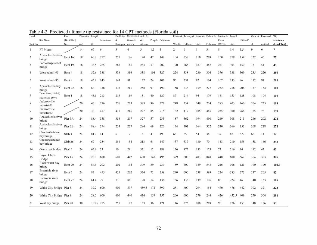
Table 4-2. Predicted ultimate tip resistance for 14 CPT methods (Florida soil) Load
Test No.Site Name
Pier (Bent/Slab) No.
Diameter
(in)
Length
(ft)Schmertmann
De-Ruiter & Beringen
Bustamante &
Gianeselli
(LCPC)
Aoki & de Alencar
Penpile Philipponnat
Prince &
Wardle
Turmay &
Fakhroo
Almeida
et al.
Eslami &
Fellenius
Jardine & Chow (MTD)
Powell
et al.UWA-05
Zhou et
al.
Proposed
method
Tip resistance (Load Test)
1 FT Myers 14 67 6 3 4 3 1.5 3 2 6 1 3 8 1.4 3.5 9 6 7
2 Apalachicola river bridge Bent 16 18 60.2 257 257 126 170 47 142 104 257 110 209 150 179 154 122 46 77
3 Port orange relief bridge Bent 19 18 33.5 265 265 186 283 57 202 170 265 187 487 221 304 159 151 51 45
4 West palm I-95 Bent 4 18 52.6 338 338 316 338 104 327 224 338 230 304 376 338 309 235 220 266
5 West palm I-95 Bent 9 18 45.8 143 143 81 137 24 102 96 251 82 164 107 133 86 112 91 261
6 Apalachicola bay bridge Bent 22 18 68 338 338 211 258 97 190 158 338 159 227 232 258 206 157 154 160
7Trout River, I-95 @
Edgewood DriveBent 1 18 48.5 213 213 119 181 40 120 89 214 94 179 141 153 128 108 104 110
8 Jacksonville industrial1 20 46 276 276 263 383 96 277 248 334 249 724 283 403 166 204 235 109
9 Jacksonville industrial2 20 36 417 417 216 297 85 215 182 417 185 485 235 300 268 185 76 159
10 Apalachicola river bridge Pier 3A 24 88.4 358 358 207 327 57 233 187 362 194 490 219 308 215 216 202 273
11 Apalachicola river bridge Pier 3B 24 88.4 254 254 227 284 69 226 174 301 164 352 240 266 153 208 218 273
12 Choctawhatchee bay bridge Slab 3 24 81.7 14 6 17 16 4 49 63 65 54 38 37 87 8.5 66 14 12
13 Choctawhatchee bay bridge Slab 26 24 69 254 254 154 213 61 149 137 337 130 70 143 210 155 158 146 242
14 Overstreet bridge Pier16 24 65.6 23 10 28 32 12 188 176 477 133 175 73 216 14 192 43 45
15 Bayou Chico Bridge Pier 15 24 26.7 600 600 442 600 148 495 379 600 403 848 448 600 562 364 383 376
16 Black water bay bridge Bent 20 24 84.9 202 202 194 309 59 239 189 300 189 543 216 306 121 190 190 169.5
17 Escambia river bridge Bent 5 24 87 455 455 202 334 72 258 240 600 238 599 224 385 273 237 265 85
18 Escambia river bridge Bent 77 24 61.4 77 77 88 128 14 136 136 135 139 196 86 224 46 140 133 105
19 White City Bridge Pier 5 24 37.2 600 600 507 459.5 172 399 281 600 294 154 470 476 442 302 321 323
20 White City Bridge Pier 8 24 28.5 600 600 440 434 159 357 266 600 279 244 426 452.5 409 279 304 281
21 West bay bridge Pier 20 30 103.6 255 255 107 163 36 121 116 275 108 289 96 176 153 148 126 53
72

73
Table 4-3. Predicted Davisson capacity for 14 CPT methods (Florida soil) Load
Test No.Site Name
Pier (Bent/Slab) No.
Diameter
(in)
Length
(ft)Schmertmann
De-Ruiter & Beringen
Bustamante &
Gianeselli
(LCPC)
Aoki & de Alencar
Penpile Philipponnat
Prince &
Wardle
Turmay &
Fakhroo
Almeida
et al.
Eslami &
Fellenius
Jardine & Chow (MTD)
Powell
et al.UWA-05
Zhou et
al.
Proposed
Method
Davisson Capacity (Load Test)
1 FT Myers 14 67 112 174 184 94 66 150.6 80.2 108 289 141 113 296 60 144 152 140
2 Apalachicola river bridge
Bent 16 18 60.2 224 237 264 169 101 224 145 219 301 212 220 333 167 315 170 165
3 Port orange relief bridge
Bent 19 18 33.5 217 198 228 213 84 264 150 187 295 290 286 334 239 265 143 103
4 West palm I-95 Bent 4 18 52.6 223 232 374 263 100 382 150 208 444 253 383 481 325 359 266 250
5 West palm I-95 Bent 9 18 45.8 166 157 273 169 82 225 132 193 351 201 220 368 155 249 225 266
6 Apalachicola bay bridge
Bent 22 18 68 205 205 305 213 97 257 125 227 425 202 257 459 189 284 245 213
7Trout River, I-95 @ Edgewood Drive
Bent 1 18 48.5 155 155 255 131 68 197 92 169 324 166 182 345 142.5 223 192 194
8 Jacksonville industrial1
20 46 242 275 434 355 121 358 201 226 451 469 487 502 360 367 358 283
9 Jacksonville industrial2
20 36 275 275 286 263 113 329 193 265 347 327 362 386 304 338 272 185
10 Apalachicola river bridge
Pier 3A 24 88.4 311 245.5 603.5 319 133 443 194.8 224.8 720 436 464 769 310.5 426 375 479
11 Apalachicola river bridge
Pier 3B 24 88.4 405 383 545 346 200 462 291 383 696 463 516 740 292 595 380 479
12 Choctawhatchee bay bridge
Slab 3 24 81.7 174 268 273 189 113 272 138 236 594 277 242 633 114 337 236 249
13 Choctawhatchee bay bridge
Slab 26 24 69 229 319 387 197 111 281 140 300 503 226 238 537 145 379 303 480
14 Overstreet bridge Pier16 24 65.6 216 252 337 288 106 353 193 375 415 310 328 453 155 424 262 250
15 Bayou Chico Bridge
Pier 15 24 26.7 283 303 378 328 97 366 181 264 380 411 383 446 403 457 329 393
16 Black water bay bridge
Bent 20 24 84.9 304 255 501 319 134 411 212 304 593 431 472 636 306 414 411 438
17 Escambia river bridge
Bent 5 24 87 468 517 792 520 188 691 284 445 831 603 695 884 442.5 559 693 425
18 Escambia river bridge
Bent 77 24 61.4 187 243 502 304 94 432 151 230 520 320 385 558 231 326 432 735
19 White City Bridge Pier 5 24 37.2 280.5 370 336 230 108 256.5 164 330 272 176.5 340 338 259 421.5 221 332
20 White City Bridge Pier 8 24 28.5 271 361 317 212 94 256 136 288 276 183 276 341 239 372 221 250
21 West bay bridge Pier 20 30 103.6 309.5 231 304 255 171 382 202 452 1009 446 326 1066 208.5 513 344 425

Table 4-4. LRFD resistance factors,Φ, for CPT methods (ultimate skin friction, Florida soil)
Analysis method λ R COV R Φ Φ/λ R
Schmertmann (1978) 1.619 0.507 0.548 0.339de Ruiter and Beringen (1979) 1.460 0.509 0.492 0.337Bustamante and Gianeselli(LCPC) (1982) 0.777 0.358 0.382 0.491Aoki & de Alencar (1975) 1.492 0.378 0.697 0.467Penpile Method (Clisby et al. 1978) 2.737 0.531 0.873 0.319Philipponnat (1980) 0.899 0.361 0.439 0.488Prince and Wardle (1982) 2.285 0.570 0.663 0.290Tumay and Fakhroo (1982) 1.653 0.537 0.520 0.314Almeida et al. (1996) 0.588 0.426 0.243 0.414Eslami & Fellenius (1997) 1.190 0.405 0.520 0.437Jardine & Chow (MTD) (1996) 0.926 0.453 0.358 0.387Powell et al. (2001) 0.582 0.423 0.243 0.418UWA-05 (2005) 1.502 0.585 0.420 0.280Zhou et al. (1982) 1.326 0.537 0.417 0.315Proposed Method (2006) 0.975 0.292 0.565 0.580
Table 4-5. LRFD resistance factors,Φ, for CPT methods (ultimate tip resistance, Florida soil)
Analysis method λ R COV R Φ Φ/λ R
Schmertmann (1978) 0.755 0.663 0.175 0.233de Ruiter and Beringen (1979) 0.986 1.023 0.106 0.107Bustamante and Gianeselli(LCPC) (1982) 1.001 0.655 0.238 0.237Aoki & de Alencar (1975) 0.795 0.669 0.182 0.229Penpile Method (Clisby et al. 1978) 3.172 0.747 0.608 0.192Philipponnat (1980) 0.879 0.714 0.182 0.207Prince and Wardle (1982) 1.090 0.745 0.210 0.193Tumay and Fakhroo (1982) 0.530 0.575 0.152 0.287Almeida et al. (1996) 1.276 1.155 0.106 0.083Eslami & Fellenius (1997) 0.823 1.054 0.083 0.101Jardine & Chow (MTD) (1996) 0.829 0.611 0.218 0.263Powell et al. (2001) 0.826 1.262 0.057 0.069UWA-05 (2005) 1.202 0.708 0.252 0.210Zhou et al. (1982) 0.885 0.567 0.259 0.293Proposed Method (2006) 1.141 0.504 0.390 0.341
74

75
Analysis method λ R COV R Φ Φ/λ R
Schmertmann (1978) 1.327 0.522 0.433 0.327de Ruiter and Beringen (1979) 1.224 0.474 0.449 0.367Bustamante and Gianeselli(LCPC) (1982) 0.852 0.309 0.473 0.555Aoki & de Alencar (1975) 1.289 0.385 0.591 0.459Penpile Method (Clisby et al. 1978) 2.869 0.478 1.045 0.364Philipponnat (1980) 0.969 0.342 0.495 0.511Prince and Wardle (1982) 1.935 0.456 0.744 0.385Tumay and Fakhroo (1982) 1.229 0.471 0.455 0.370Almeida et al.
Table 4-6. LRFD resistance factors,Φ, for CPT methods (Davisson capacity, Florida soil)
(1996) 0.692 0.396 0.309 0.447Eslami & Fellenius (1997) 1.094 0.446 0.430 0.394Jardine & Chow (MTD) (1996) 0.982 0.415 0.419 0.426
0.375 0.295 0.471Powell et al. (2001) 0.628UWA-05 (2005) 1.492Zhou et al. (1982) 0.873Proposed Method (2006) 1.079
0.516 0.494 0.3310.436 0.353 0.4040.267 0.665 0.617

Table 4-7. Predicted ultimate skin friction for 14 CPT methods (Louisiana soil) Load Test No.
Site NamePier (Bent/Slab) No.
Diameter
(in)
Length
(ft)
Schmertmann
De-Ruiter
&
Beringen
Bustamante &
Gianeselli
(LCPC)
Aoki &
de
Alencar
Penpile Philipponnat
Prince &
Wardle
Turmay &
Fakhroo
Almeida
et al.
Eslami &
Fellenius
Jardine &
Chow
(MTD)
Powell
et al.
UWA-05
Zhou et
al.
Proposed
Method
Skin Friction
(Load Test)1 Houma_ICW_Bridge TP 1 14 80 181 187 208 87 83 132 111 153 221 192 115 230 55 208 132 106.42 Houma_ICW_Bridge TP 2 14 70 99 201 164 47 59 89 66 117 129 110 86 140 29.5 158 89 433 Houma_ICW_Bridge TP 3 14 80 140 159 140 68 68 108 84.5 147 174 176 107 182 42 178 108 116.54 Houma_ICW_Bridge TP 4 14 81 123 156 138 57 61 93 71 151 136.5 140 83 145 36 175 93 1055 Bayou_Boeuf_Main_Span TP 2 14 70 89 227 151 45 50 106 53 120 149 141 85 161 36 142 106 976 Bayou_Boeuf_Main_Span TP 5 14 80 59 150 105 42 32 72 30 161 96 147 64.5 104 27 109 72 115
7 Bayou_Boeuf_West_Approach TP 1 14 89.5 131 177 119 56 76.5 90 82 131 120 131 85 131 31 206 90 105
8 Bayou_Boeuf_West_Approach TP 3 14 63.5 91 138 115 46 53 80.5 60 107 119 130 72 126 43 145 80.5 125.5
9 Bayou_Boeuf_East_Approach F 1 14 68 88.5 138.5 87.5 47.5 51 69 52 107 92 142 59 100 25 146 69 90
10 Bayou_Boeuf_East_Approach F 2 14 71 91 131 86 40 50 63 50 116 87 122 60 95 24 149 63 90
11 Bayou_Boeuf_East_Approach F 3 14 77.5 99 176.5 113 50 55 87 56 129 117 149.5 76 128 30 164 87 82
12 Bayou_Boeuf_East_Approach F 4 14 79 107.5 248 181 58 59 114 60 125 157 148 94 171 36 171 114 95
13 Bayou_Boeuf_East_Approach F 5 14 79 96 185 113 40 53 81 53 135.5 130 168 75 142 31 161 81 70
14 Houma_ICW_Bridge TP 5 16 71.5 111 127 88 44 62.5 64 64 126 85 106 65 93 23 180 64 85
15 Bayou_Boeuf_West_Approach TP 4 16 70 126 166 140 66 79 102 98 129 140 152 90 149 37 203 102 80
16 Bayou_Ramos_Bridge TP 1 16 78 118 163 136 59 65 101 68 148 165 158 88 175 43 186 101 9817 Bayou_Ramos_Bridge TP 7 16 77 129 169 126 61 71 103 78 140 136 149 89 145.5 34 198 98 107.618 Houma 18 105 187 316 202.5 102 102 173 106 215 248.5 257 146 268 52 294 173 16019 Tickfaw_River_Bridge TP 1 30 59.3 283 606 412 145 170 286 238 251 387 307.5 280 418 67 396 286 407
20 Bayou_Boeuf_West_Approach TP 2 30 110 429 492 374.5 170 242 278 281 344 437 387 301 473 83 625 278 285
21 Bayou_Ramos_Bridge TP 2 30 88 437 407 523 198 213 398 283 343 617 442 354 635 156 497 398 36522 Bayou_Ramos_Bridge TP 3 30 104 453 551 466 253 256 490 341 406 778 500 380 805 141 603 490 35323 Bayou_Ramos_Bridge TP 4 30 99.3 464 542 451 212 213 497 285 411 614 444 393 641 188 523 497 45424 Bayou_Ramos_Bridge TP 5 30 113 434 557 375 208 217 345 267 404 421 456 365 452 170 584 345 307
25 Bayou_Boeuf_East_Approach F 6 30 110 332 676 487 154 186 213.5 197 378.5 440 519 311 479 73.5 532 313.5 280
26 Gibson_Raceland_ Highway TP 1 30 116 319 553 377 169 169 315 175 435 428 455 300 463.5 93 504 315 364
27 Gibson_Raceland_ Highway TP 4 30 124 412 648 447 211 203 400 245.5 505 521 526 358 559 135 573 400 387
28 Luling_Bridge 30 112 491 516 408 209 228 420.5 311 500 698 582 362 724 160 582 420.5 424
76

Table 4-8. Predicted ultimate tip resistance for 14 CPT methods (Louisiana soil) Load Test No.
Site NamePier (Bent/Slab) No.
Diameter
(in)
Length
(ft)
Schmertmann
De-Ruiter
&
Beringen
Bustamante &
Gianeselli
(LCPC)
Aoki &
de
Alencar
Penpile Philipponnat
Prince &
Wardle
Turmay &
Fakhroo
Almeida
et al.
Eslami &
Fellenius
Jardine &
Chow
(MTD)
Powell
et al.
UWA-05
Zhou et
al.
Proposed
Method
Tip
Resistance
(Load Test)1 Houma_ICW_Bridge TP 1 14 80 14 6 9 8.5 4 7 5 14 3 12 20 5 8 16 15 32.62 Houma_ICW_Bridge TP 2 14 70 5 2 5.5 6 4 3.5 4 5 2 3 12 3 3 10 9 123 Houma_ICW_Bridge TP 3 14 80 12 5 8 8 3 7 5 12 3 11 21 5 7 15 14 84 Houma_ICW_Bridge TP 4 14 81 11 5 7 7 3 6 4 11.5 2 9 16 3 7 14 125 Bayou_Boeuf_Main_Span TP 2 14 70 24 11 29.5 26 15 19 16 26 16 31 61 25 14 31 21 196 Bayou_Boeuf_Main_Span TP 5 14 80 2.5 1 8 5 3 4 3 2.5 1 1 18 2 1.5 9 8
7 Bayou_Boeuf_West_Approach TP 1 14 89.5 9.5 4 6.5 11 2 18 7 16 4 13.5 14 7 6 19 18.5
8 Bayou_Boeuf_West_Approach TP 3 14 63.5 93.5 93.5 62.5 64.5 22 55 39.5 98 40 64 83 64 56 52 45 39.5
9 Bayou_Boeuf_East_Approach F 1 14 68 15 7 10 9 4 8 6 15 4 13.5 21.5 6 9 17 16
10 Bayou_Boeuf_East_Approach F 2 14 71 12 5 8 8 3 7 5 12 3 10 17 5 7 14.5 13
11 Bayou_Boeuf_East_Approach F 3 14 77.5 12 5 8 7 4 6.5 5 12 3 10 18 4 7 14 13
12 Bayou_Boeuf_East_Approach F 4 14 79 19.5 9 13 12 6 9.5 7 19.5 5.5 17 29 9 12 19 9
13 Bayou_Boeuf_East_Approach F 5 14 79 12 6 9 8 3.6 7 5 12 3 11 19 5 7 15 14
14 Houma_ICW_Bridge TP 5 16 71.5 11 5 8 7 3 6 4 11 2 9 17.5 3 7 15 12
15 Bayou_Boeuf_West_Approach TP 4 16 70 17 8 11 12 4 9 7 17 5 15 24 8 10 20 18
16 Bayou_Ramos_Bridge TP 1 16 78 48 48 23 47 6.4 28 29 70 25.5 66 30 41 29 40 31 4317 Bayou_Ramos_Bridge TP 7 16 77 15 7 15 12 5 10 7 15 5 12 35.5 8.6 9 21 10 8.418 Houma 18 105 24 11 17 17 7 14 10 25 6 21 37 9 15 28 28 5619 Tickfaw_River_Bridge TP 1 30 59.3 122 55 90 79 38 68.5 48.5 125 43 116 195 69 73 123 61 77
20 Bayou_Boeuf_West_Approach TP 2 30 110 113 113 123 119 48 88 73 117 67 150.5 101 109 68 146 88
21 Bayou_Ramos_Bridge TP 2 30 88 212 212 107 252 15 155 154 212 155 380 95 250 127 168 177 16222 Bayou_Ramos_Bridge TP 3 30 104 183 183 151 173 56 131 106 187 102 246 113 166 110 199 125 14723 Bayou_Ramos_Bridge TP 4 30 99.3 78 78 151 315 29 175 193 264.5 176.5 439 141 286 47 268 175 14624 Bayou_Ramos_Bridge TP 5 30 113 455 455 381 511 163 452 313 729 296 303 359 480 273 378 336 268
25 Bayou_Boeuf_East_Approach F 6 30 110 97 44 67 60 27 46 97 100 24 90 145 39 58 96 46
26 Gibson_Raceland_ Highway TP 1 30 116 252 252 170 322 58 220 197 521 164 162 162.5 265 151 246.5 193 275
27 Gibson_Raceland_ Highway TP 4 30 124 310 310 302 414.5 90 310 254 668 217 211.5 260 352 186 359 252 254
28 Luling_Bridge 30 112 378.5 378.5 396 641 54 390 392.5 937.5 330 383 347 534 227 396 372 76
77

78
Table 4-9. Predicted ultimate pile capacity for 14 CPT methods (Louisiana soil) Load Test No.
Site NamePier (Bent/Slab) No.
Diameter
(in)
Length
(ft)
Schmertmann
De-Ruiter
&
Beringen
Bustamante &
Gianeselli
(LCPC)
Aoki &
de
Alencar
Penpile Philipponnat
Prince &
Wardle
Turmay &
Fakhroo
Almeida
et al.
Eslami &
Fellenius
Jardine &
Chow
(MTD)
Powell
et al.
UWA-05
Zhou et
al.
Proposed
Method
Ultimate
Capacity
(Load Test)
1 Houma_ICW_Bridge TP 1 14 80 195 194 217 95 87 135 117 167 224 204 134.8 235 63 224 147 1392 Houma_ICW_Bridge TP 2 14 70 104 203 170 53 62 92 70 122 131 113 98 143 32 168 98 553 Houma_ICW_Bridge TP 3 14 80 151.5 164 148 76 71.5 115.5 89 159 177 187 128.5 187 49 193 122 1254 Houma_ICW_Bridge TP 4 14 81 135 161 145 64 64 99 75 162 139 149 98 148 43 189 105 1055 Bayou_Boeuf_Main_Span TP 2 14 70 113 237 181 71.5 65.5 125 69 146 164 171 146 186 50 174 127 1166 Bayou_Boeuf_Main_Span TP 5 14 80 61 151 113.5 47 36 76 33 164 97 148 83 107 28.5 118 80 115
7 Bayou_Boeuf_West_Approach TP 1 14 89.5 140 182 125 67 79 108 88.5 146.5 124 144 99 138 37 224 109 105
8 Bayou_Boeuf_West_Approach TP 3 14 63.5 184 231 178 110 75 136 100 205 159 194 156 191 99 197 126 165
9 Bayou_Boeuf_East_Approach F 1 14 68 103 145 97 57 55 77 58 122 96 155 80 107 33.6 163 85 90
10 Bayou_Boeuf_East_Approach F 2 14 71 103 136 94 48 53 70 55 129 90 133 77 100 31 163 76 90
11 Bayou_Boeuf_East_Approach F 3 14 77.5 111 182 121 57 59 94 60.5 141 120 160 94 132 37 178 100 82
12 Bayou_Boeuf_East_Approach F 4 14 79 127 257 194 70 65 123 68 144 163 165 123 180 48 191 123 95
13 Bayou_Boeuf_East_Approach F 5 14 79 108 190 122 48 56.5 88 58 148 133.5 179 93 146.5 39 176 95 70
14 Houma_ICW_Bridge TP 5 16 71.5 122 132 95.5 50 66 69.5 68.5 138 87 115 82 96 29 195 76 85
15 Bayou_Boeuf_West_Approach TP 4 16 70 143 174 151 78 83.5 111 105 146.5 145 166.5 113 157 47 223 120 80
16 Bayou_Ramos_Bridge TP 1 16 78 167 211 159 107 72 130 97 218 190 224 118 216 72 227 132 14017 Bayou_Ramos_Bridge TP 7 16 77 144 175.5 142 73 76 113 85 155 141 161 124.5 154 43 219 108 11618 Houma 18 105 211 327 220 119 109 186 116.5 240 254 278 183 277 66 322 201 21619 Tickfaw_River_Bridge TP 1 30 59.3 405 660.5 502 224 207.5 355 287 376 430 424 475 487 140 519 347 484
20 Bayou_Boeuf_West_Approach TP 2 30 110 542 606 497.5 289 290 366 354 461.5 505 538 402 582 151 771 367 285
21 Bayou_Ramos_Bridge TP 2 30 88 649 618 636 449 228 553 437 556 772 822 449 885 283 665 575 52722 Bayou_Ramos_Bridge TP 3 30 104 636 735 617 426 312 554 447 593 880 746 493 971 251 802 615 50023 Bayou_Ramos_Bridge TP 4 30 99.3 542 620 602 527 241 672 478 676 790 883 533.5 927 235 791 672 57824 Bayou_Ramos_Bridge TP 5 30 113 889 1012 756 719 381 796 579.5 1133 717.5 759 724.5 932 443 962 681 577
25 Bayou_Boeuf_East_Approach F 6 30 110 429.5 720 554 214 213 360 234 478 464 609 456 518 132 628 360 280
26 Gibson_Raceland_ Highway TP 1 30 116 571 805 547.5 491 227 535 372 955.5 592 617 463 729 245 750 508 639
27 Gibson_Raceland_ Highway TP 4 30 124 722 958 749 626 293 710 499 1173 738.5 738 618 911 321 932 652 641
28 Luling_Bridge 30 112 870 895 804 850 282 810 704 1438 1027 965 709 1258 387 978 793 500

Table 4-10. LRFD resistance factors,Φ, for CPT methods (ultimate skin friction, Louisiana soil)
Analysis method λ R COV R Φ Φ/λ R
Schmertmann (1978) 0.910 0.322 0.489 0.537de Ruiter and Beringen (1979) 0.608 0.269 0.373 0.613Bustamante and Gianeselli(LCPC) (1982) 0.800 0.255 0.507 0.634Aoki & de Alencar (1975) 1.846 0.239 1.218 0.660Penpile Method (Clisby et al. 1978) 1.690 0.315 0.924 0.547Philipponnat (1980) 1.053 0.248 0.679 0.645Prince and Wardle (1982) 1.504 0.378 0.703 0.467Tumay and Fakhroo (1982) 0.803 0.283 0.476 0.593Almeida et al. (1996) 0.734 0.282 0.436 0.594Eslami & Fellenius (1997) 0.713 0.259 0.448 0.628Jardine & Chow (MTD) (1996) 1.145 0.240 0.752 0.657Powell et al. (2001) 0.684 0.275 0.413 0.604UWA-05 (2005) 2.983 0.306 1.667 0.559Zhou et al. (1982) 0.614 0.290 0.357 0.582Proposed Method (2006) 1.040 0.248 0.670 0.644
Table 4-11. LRFD resistance factors,Φ, for CPT methods (ultimate tip resistance, Louisiana soil)
Analysis method λ R COV R Φ Φ/λ R
Schmertmann (1978) 1.073 0.678 0.241 0.224de Ruiter and Beringen (1979) 1.869 1.000 0.209 0.112Bustamante and Gianeselli(LCPC) (1982) 1.342 0.728 0.269 0.200Aoki & de Alencar (1975) 1.133 0.910 0.152 0.135Penpile Method (Clisby et al. 1978) 4.024 0.727 0.807 0.201Philipponnat (1980) 1.519 0.856 0.229 0.151Prince and Wardle (1982) 1.864 0.937 0.237 0.127Tumay and Fakhroo (1982) 0.876 0.844 0.136 0.155Almeida et al. (1996) 2.721 1.163 0.224 0.082Eslami & Fellenius (1997) 1.168 0.913 0.156 0.134Jardine & Chow (MTD) (1996) 0.941 0.590 0.261 0.277Powell et al. (2001) 1.710 1.176 0.137 0.080UWA-05 (2005) 1.794 0.678 0.403 0.225Zhou et al. (1982) 0.889 0.578 0.253 0.285Proposed Method (2006) 1.107 0.447 0.435 0.393
79

Table 4-12. LRFD resistance factors,Φ, for CPT methods (ultimate pile capacity, Louisiana soil)
Analysis method λ R COV R Φ Φ/λ R
Schmertmann (1978) 0.838 0.320 0.452 0.539de Ruiter and Beringen (1979) 0.613 0.257 0.387 0.631Bustamante and Gianeselli(LCPC) (1982) 0.776 0.250 0.498 0.641Aoki & de Alencar (1975) 1.417 0.280 0.845 0.596Penpile Method (Clisby et al. 1978) 1.740 0.312 0.958 0.551Philipponnat (1980) 0.985 0.231 0.663 0.673Prince and Wardle (1982) 1.376 0.372 0.652 0.474Tumay and Fakhroo (1982) 0.698 0.263 0.434 0.622Almeida et al. (1996) 0.766 0.266 0.473 0.618Eslami & Fellenius (1997) 0.676 0.246 0.438 0.648Jardine & Chow (MTD) (1996) 0.971 0.222 0.668 0.687Powell et al. (2001) 0.678 0.260 0.424 0.626UWA-05 (2005) 2.317 0.276 1.396 0.603Zhou et al. (1982) 0.597 0.286 0.351 0.587Proposed Method (2006) 0.964 0.230 0.649 0.673
80

Archer Landfill
0
5
10
15
20
25
30
35
40
45
0 100 200 300 400Qc(tsf)
Dep
th(ft
)
DTP T1DTP T2CPT
Figure 4-1. CPT and DTP test data from Archer Landfill site
81

Archer Landfill
0
5
10
15
20
25
30
35
40
45
0 1 2 3 4 5F. R. (%)
Dep
th (f
t)
DTPCPT
Figure 4-2. Friction ratio of CPT and DTP rest from Archer Landfill site
82

Slightly Silty Fine Sand to Fine Sand
Dense Silty Fine Sand
Clay
Slightly Silty Fine Sand to Fine Sand
Slightly Silty Fine Sand to Fine Sand
Dense Silty Fine SandDense Silty Fine Sand
Clay
I-95 @ Edgewood
0
10
20
30
40
50
60
0 100 200 300 400Qc (tsf)
Dep
th (f
t)
DTP T1DTP T2CPT
Figure 4-3. CPT and DTP test data from I–95 at Edgewood Avenue site
83

I-95 @ Edgewood
0
10
20
30
40
50
60
0 1 2 3 4 5F.R.(%)
Dep
th (f
t)
DTPCPT
Figure 4-4. Friction ratio of CPT and DTP test from I–95 at Edgewood Avenue site
84

I-95 @ Edgewood
0
10
20
30
40
50
60
0 0.5 1 1.5 2Tip2/Tip1
Dep
th (f
t)
DTP
I-95 @ Edgewood
0
10
20
30
40
50
60
0 5 10 15Qc/N
Dep
th (f
t)
DTPCPT
Figure 4-5. Tip2/Tip1 ratio and Qc/N ratio of CPT and DTP test from I–95 at Edgewood Avenue site
85

Apalachicola River Bridge Pier 3
0
10
20
30
40
50
60
70
80
90
100
0 100 200 300
Tip Resistance(tsf)
Dep
th (f
t)Tip 1Tip 2CPT
Lightly Cemented Sand
Lightly Cemented Sand layer
Sandy Silt
Silty Clay
Lightly Cemented Sand
Lightly Cemented Sand
Lightly Cemented Sand layer
Lightly Cemented Sand layer
Sandy Silt
Silty Clay
Lightly Cemented Sand
Figure 4-6. CPT and DTP test data from Apalachicola River Bridge site
86

0
10
20
30
40
50
60
70
80
90
100
0 0.5 1 1.5
Tip 2/Tip 1
Dep
th (
ft)Apalachicola River Bridge Pier 3
0
10
20
30
40
50
60
70
80
90
100
0 5 10 15 20
Qc/N
Dep
th (f
t)
DTP
CPT
Lightly Cemented Sand
LightlyCemented Sand
Sandy Silt
Silty Clay
LightlyCemented Sand
Lightly Cemented Sand
LightlyCemented Sand
LightlyCemented Sand
Sandy Silt
Silty Clay
LightlyCemented Sand
Figure 4-7. Tip2/Tip1 ratio and Qc/N ratio of CPT and DTP test from Apalachicola River Bridge site
87

West Bay Bridge, DTP vs CPTs
0
10
20
30
40
50
60
70
80
90
100
110
120
130
140
150
160
0 50 100 150 200 250
Tip Resistance (tsf)
Dep
th
(ft)
DTP T1DTP T2CPT1CPT2
Lightly Cemented Sand layer
Well Cemented Sand
West Bay Bridge, DTP vs CPTs
0
10
20
30
40
50
60
70
80
90
100
110
120
130
140
150
160
0 50 100 150 200 250
Tip Resistance (tsf)
Dep
th
(ft)
DTP T1DTP T2CPT1CPT2
Lightly Cemented Sand layer
Well Cemented Sand
Figure 4-8. CPT and DTP test data from West Bay Bridge site
88

0
10
20
30
40
50
60
70
80
90
100
110
120
130
140
150
0 0.5 1 1.5Tip2/Tip1
Dep
th (f
t)
Lightly Cemented Sand layer
Cemented Sand layer
DTP T1
0
10
20
30
40
50
60
70
80
90
100
110
120
130
140
150
0 5 10 15 20
T1/N
Dep
th (ft)
Figure 4-9. Tip2/Tip1 ratio and Qc/N ratio of CPT and DTP test from West Bay Bridge site
89

0
5
10
15
20
25
30
35
40
45
0 100 200 300 400 500Tip Bearing (TSF)
Dep
th (f
t)
DTP Tip1DTP Tip2CPT
Well Cemented Sand
Clayey Silt
WellCemented Sand
Lightly Cemented Sand
Well Cemented Sand
Clayey Silt
WellCemented Sand
Lightly Cemented Sand
Figure 4-10. CPT and DTP test data from Port Orange Relief Bridge site
90

0
5
10
15
20
25
30
35
40
45
0 5 10 15 20Qc/N
Dep
th (f
t)
DTPCPT
Tip2/Tip1
0
5
10
15
20
25
30
35
40
45
0 0.5 1 1.5
Dep
th (f
t)
Well Cemented Sand
Clayey Silt
WellCemented Sand
Lightly Cemented Sand
Well Cemented Sand
Clayey Silt
WellCemented Sand
Lightly Cemented Sand
Figure 4-11. Tip2/Tip1 ratio and Qc/N ratio of CPT and DTP test from Port Orange Relief Bridge site
91

Well Cemented Sand
Clayey Silt with Shell
Well Cemented Sand
Clay
Sand
University of Central Florida
0
10
20
30
40
50
60
70
0 100 200
Qc(tsf)
Dep
th(ft
)
DTP T1DTP T2CPT
Well Cemented Sand Lightly Cemented Sand Sand
Well Cemented Sand
Clay
Lightly Cemented Sand
Figure 4-12. CPT and DTP test data at the University of Central Florida site
92

0
5
10
15
20
25
30
35
40
45
50
55
60
65
70
0 0.5 1 1.5
Tip2/Tip1
Dep
th
(ft)
0
10
20
30
40
50
60
70
0 5 10 15 20
Qc/N
Dep
th(ft
)
CPT, Qc/N
Well Cemented Sand
Lightly Cemented Sand
Figure 4-13. Tip2/Tip1 ratio and Qc/N ratio of CPT and DTP test at the University of Central Florida site
93

Lightly Cemented Sand
I-295 @ Blanding Blvd
0
10
20
30
40
50
60
70
0 100 200 300 400
Qc(tsf)
Dep
th(ft
DTP T1DTP T2CPT
Lightly Cemented Sand
I-295 @ Blanding Blvd
0
10
20
30
40
50
60
70
0 100 200 300 400
Qc(tsf)
Dep
th(ft
DTP T1DTP T2CPT
I-295 @ Blanding Blvd
0
10
20
30
40
50
60
70
0 100 200 300 400
Qc(tsf)
Dep
th(ft
DTP T1DTP T2CPT
Figure 4-14. CPT and DTP test data at I-295 at Blanding Blvd site
94

T2/ T1
0
5
10
15
20
25
30
35
40
45
50
55
60
0 0.5 1 1.5 2
Dep
th(ft
0
5
10
15
20
25
30
35
40
45
50
55
60
0 5 10 15 20
Qc/N
Dep
th(ft
DTP
CPT
Lightly Cemented Sand
T2/ T1
0
5
10
15
20
25
30
35
40
45
50
55
60
0 0.5 1 1.5 2
Dep
th(ft
0
5
10
15
20
25
30
35
40
45
50
55
60
0 5 10 15 20
Qc/N
Dep
th(ft
DTP
CPT
Lightly Cemented Sand
Figure 4-15. Tip2/Tip1 ratio and Qc/N ratio of CPT and DTP test at I-295 at Blanding Blvd site
95

Tip Resistance
0
5
10
15
20
25
30
35
40
45
0 100 200 300 400Qc (tsf)
Dep
th (f
t) `
DTP T1DTP T2CPT
Lightly Cemented Sand
Tip Resistance
0
5
10
15
20
25
30
35
40
45
0 100 200 300 400Qc (tsf)
Dep
th (f
t) `
DTP T1DTP T2CPT
Lightly Cemented Sand
Lightly Cemented Sand
Figure 4-16. CPT and DTP test data at I-295 at Normandy Blvd. site
96

0
5
10
15
20
25
30
35
40
45
0 5 10 15 20Qc/N
Dept
h (ft
)
DTP
CPT
Tip2/Tip1
0
5
10
15
20
25
30
35
40
45
0 0.5 1 1.5
Dep
th (f
t)
Lightly Cemented Sand
0
5
10
15
20
25
30
35
40
45
0 5 10 15 20Qc/N
Dept
h (ft
)
DTP
CPT
Tip2/Tip1
0
5
10
15
20
25
30
35
40
45
0 0.5 1 1.5
Dep
th (f
t)
Lightly Cemented Sand
Figure 4-17. Tip2/Tip1 ratio and Qc/N ratio of CPT and DTP test at I-295 at Normandy Blvd. site
97

Lightly Cemented Sand
Sandy Clay
Silty Sand
Lightly Cemented Sand
Clay Silty Sand
Clay
White City Bridge-Pier 5
0
5
10
15
20
25
30
35
40
0 50 100 150 200
Qc(tsf)
Dep
th (f
t) DTP T1DTP T2CPT
Lightly Cemented Sand
Figure 4-18. CPT and DTP test data in White City site (pier 5)
98

0
5
10
15
20
25
30
35
40
0 0.5 1 1.5
Tip2/Tip1
Dep
th (f
t)
White City Bridge-Pier 5
0
5
10
15
20
25
30
35
40
0 5 10 15 20
Qc/N
Dep
th(ft
)
DTPCPT
Lightly Cemented Sand
Figure 4-19. Tip2/Tip1 ratio and Qc/N ratio of CPT and DTP test in White City site (pier 5)
99

White City Bridge-Pier 8
0
5
10
15
20
25
30
35
40
0 50 100 150 200 250 300 350 400
Qc(tsf)
Dep
th (f
t) DTP T1DTP T2CPT
Lightly Cemented Sand
Silty Sand
Lightly Cemented Sand
Clay
Lightly Cemented Sand
Sand
Figure 4-20. CPT and DTP test data in White City site (pier 8)
100

Figure 4-21. Tip2/Tip1 ratio and Qc/N ratio of CPT and DTP test in White City site (pier 8)
0
5
10
15
20
25
30
35
40
0 0.5 1 1.5
Tip2/Tip1D
epth
(ft)
White City Bridge-Pier 8
0
5
10
15
20
25
30
35
40
-5 0 5 10 15 20
Qc/N
Dep
th(ft
)
DTPCPTLightly
Cemented Sand
101

Bayou_Boeuf_East_Approach_F4
0.00
20.00
40.00
60.00
80.00
100.00
120.00
0.0 0.2 0.4 0.6 0.8 1.0 1.2 1.4 1.6 1.8 2.0Displacement (in)
Load
(ton
s)
Q Davisson
Figure 4-22. Typical load test curve in Louisiana soil
102

0
0.5
1
1.5
2
2.5
3
3.5
4
1 2 3 4 5 6 7 8 9 10 11 12 13 14 15 16 17 18 19 20 21Case No.
λ i
Schmertmann Method de-Ruiter & Beringen Method LCPC MethodAoki & Alencar Method Penpile Method Philipponnat MethodPrince & Wardle Method Turmay & Fakhroo Method Almeida et al. MethodEslami & Fellenius Method Jardine & Chow Method Powell et al. MethodUWA-05 Method Zhou et al. Method Proposed Method
0
0.2
0.4
0.6
0.8
1
1.2
1.4
1.6
1.8
2
1 2 3 4 5 6 7 8 9 10 11 12 13 14 15 16 17 18 19 20 21Case No.
λ i
Schmertmann Method de-Ruiter & Beringen Method LCPC MethodAoki & Alencar Method Penpile Method Philipponnat MethodPrince & Wardle Method Turmay & Fakhroo Method Almeida et al. MethodEslami & Fellenius Method Jardine & Chow Method Powell et al. MethodUWA-05 Method Zhou et al. Method Proposed Method
Figure 4-23. Comparisons (ratio: measured/predicted) for 14 methods using Florida soil. A) Y- scale from 0 to 4. B) Y-scale from 0 to 2.
103

0
0.5
1
1.5
2
2.5
3
3.5
4
1 2 3 4 5 6 7 8 9 10 11 12 13 14 15 16 17 18 19 20 21 22 23 24 25 26 27 28Case No.
λ i
Schmertmann Method de-Ruiter & Beringen Method LCPC MethodAoki & Alencar Method Penpile Method Philipponnat MethodPrince & Wardle Method Turmay & Fakhroo Method Almeida et al. MethodEslami & Fellenius Method Jardine & Chow Method Powell et al. MethodUWA-05 Method Zhou et al. Method Proposed Method
00.20.40.60.8
11.21.41.61.8
2
1 2 3 4 5 6 7 8 9 10 11 12 13 14 15 16 17 18 19 20 21 22 23 24 25 26 27 28Case No.
λ i
Schmertmann Method de-Ruiter & Beringen Method LCPC MethodAoki & Alencar Method Penpile Method Philipponnat MethodPrince & Wardle Method Turmay & Fakhroo Method Almeida et al. MethodEslami & Fellenius Method Jardine & Chow Method Powell et al. MethodUWA-05 Method Zhou et al. Method Proposed Method
Figure 4-24. Comparisons (ratio: measured/predicted) for 14 methods using Louisiana soil. A) Y- scale from 0 to 4. B) Y-scale from 0 to 2.
104

0.6 0.8 1 1.2 1.4 1.60
0.5
1
1.5
2
Mean = 1.079
Stdev = 0.288
Figure 4-25. Frequency of λ of the proposed method for Florida soil
0.83 0.87 0.91 0.96 1 1.04 1.08 1.12 1.16 1.2 1.25 1.29 1.33 1.370
2
4
6 Mean = 1.079
Stdev = 0.061
Figure 4-26. Frequency of the sample means using Bootstrap method for Florida soil (100,000
re-sampling runs, the proposed method)
105

0.11 0.13 0.16 0.18 0.21 0.23 0.26 0.28 0.31 0.33 0.36 0.38 0.410
2
4
6
8Mean = 0.278
Stdev = 0.042
Figure 4-27. Frequency of the sample standard deviations using Bootstrap method for Florida
soil (100,000 re-sampling runs, the proposed method)
0.4 0.48 0.57 0.65 0.74 0.82 0.91 0.99 1.08 1.16 1.25 1.33 1.420
0.5
1
1.5
2
2.5
Mean = 0.963
Stdev = 0.224
Figure 4-28. Frequency of λ of the proposed method for Louisiana soil
106

0.8 0.82 0.85 0.87 0.9 0.92 0.94 0.97 0.99 1.01 1.04 1.06 1.09 1.110
2
4
6
8
10
Mean = 0.963
Stdev = 0.042
Figure 4-29. Frequency of the sample means using Bootstrap method for Louisiana soil (100,000
re-sampling runs, the proposed method)
0.1 0.12 0.14 0.15 0.17 0.19 0.21 0.22 0.24 0.26 0.28 0.29 0.310
5
10
Mean = 0.219
Stdev = 0.027
Figure 4-30. Frequency of the sample standard deviations using Bootstrap method for Louisiana
soil (100,000 re-sampling runs, the proposed method)
107

0 0.31 0.62 0.92 1.23 1.54 1.85 2.15 2.46 2.77 3.08 3.38 3.69 40
0.5
1
1.5
Mean = 1.327
Stdev = 0.693
Figure 4-31. Frequency of λ of the Schmertmann method for Florida soil
0.9 1 1.1 1.2 1.3 1.4 1.5 1.6 1.7 1.8 1.9 2 2.11 2.210
0.5
1
1.5
2
2.5 Mean = 1.328
Stdev = 0.148
Figure 4-32. Frequency of the sample means using Bootstrap method for Florida soil (100,000 re-sampling runs, Schmertmann method)
108

0.13 0.23 0.33 0.43 0.53 0.63 0.73 0.83 0.93 1.03 1.13 1.23 1.33 1.430
1
2
3
Mean = 0.631
Stdev = 0.243
Figure 4-33. Frequency of the sample standard deviations using Bootstrap method for Florida soil (100,000 re-sampling runs, Schmertmann method)
109

CHAPTER 5 CONCLUSION
Conclusion
A total of 21 cases (load test data with CPT close to it) in Florida and 28 cases in Louisiana
have been used to assess LRFD resistance factor, Φ, for 14 pile axial capacity prediction
methods based on CPT results. One of the best methods, the Philipponnat method, was chosen
and modified to form the proposed UF method. Ten field sites were revisited with paired CPT
and DTP tests performed. This was an attempt to develop identifiers for cemented sand, which is
the one of the most challenging soil types for geotechnical engineers.
Based on the analysis of the test data and resistance factors of each method, the following
conclusions can be drawn:
• Current pile axial capacity prediction methods using CPT results overestimate pile capacities in cemented soil. This issue needs to be addressed with additional testing.
• The proposed procedure for separating skin friction and tip resistance is a useful
tool to better evaluate the pile capacity prediction methods. • Of the fourteen pile axial capacity prediction methods analyzed, the Philipponnat
method, LCPC method and MTD method were shown to have the highest Φ/λ value, indicating more accurate results.
• The proposed UF method has the highest Φ/λ for Florida soil and second highest
for Louisiana soil (0.62 for Florida soil and 0.67 for Louisiana soil) among all the methods. In addition, it has the lowest coefficient of variation for Florida soil and second lowest for Louisiana soil (0.27 for Florida soil and 0.23 for Louisiana soil). Therefore, the proposed UF method works very well for both sands (Florida soil) and clays (Louisiana soil). (Hu et al. 2007a)
• The dual tip penetrometer can be a potential tool to identify cemented soil by using
the identifier, T2/T1. The ranges of T2/T1 for different soil type are shown below, based on limited test data (10 cases) and more data need to be collected to confirm these figures. (Hu et al. 2007b) ≈ 0.5 Non-Cemented Sand (Loose and Medium Dense Sand)
= 0.3~0.5 Lightly Cemented Sand ≈ 1 Strongly Cemented Sand,
110

= 0.5~1 Silty Sand, Sandy Silt and Silty Clay < 0.5 Highly Sensitive Clay > 1 Dense Silty Sand ≥1 Clayey Silt, Silty Clay and Clay
• Using the bootstrap method on field data shows that the standard deviation of the resampled mean and resampled standard deviation are quite small for the proposed method. This means that the proposed method provides higher quality predictions.
Future Work
There still needs work to confirm the above conclusions. For example:
• Since the sleeve friction reading of DTP is not identical to CPT and it hinders the ability of DTP to identify soil type, a redesign of DTP is recommended to eliminate the influence of the second tip to the sleeve friction.
• More bridge sites should be revisited and tested with both the CPT and DTP.
Table 5-1 shows the bridge sites where load test data are available. • Validate the cemented sand identification values from the DTP (T1/T2), and
compare them with SPT & CPT data. • Evaluate the proposed pile capacity method based on a larger CPT, DTP, and load
test database. This will provide confidence in recommending a realistic LRFD resistance factor, Φ, and in turn further the stage of geotechnical engineering practice.
111

Table 5-1. Bridge sites where load test data are available
Cemented Sand SiteLoad Test
No.Site Name Project Number
Pier (Bent/Slab) No.
StationPile
Embeded
Length (ft)
Desired
CPT
Depth (ft)1 T-1 N1533290 E631461 46 532 T-6 N1533447 E631541 67 723 T-7 N153325 E631568 46.2 534 T-14 N1533572 E631617 36 435 TP-2 N/A 33 386 TP-10 N/A 63 687 Siesta Key Sarasota N/A N/A N/A 16.3 20.38 3A N/A 36.5 449 3B N/A 46 5310 3C N/A 60 6511 B-20 N2909 W6492 64 7012 B-21 N4080 W6905 46 5313 B-4 (Pier-4) 264+27.23 52.6 5914 B-9 (Pier-9) 271+25.67 45.8 5215 C-2 (Pier-2) 1981+87.41 43 49
Non-Cemented Sand SiteLoad Test
No.Site Name Project Number
Pier (Bent/Slab) No.
StationPile Embeded Length (ft)
Desired CPT Depth (ft)
1 TP-1 240+10 41.2 502 TP-38 378+29 23.6 323 Pile #2 N/A 64 684 Pile#3 N/A 49.2 585 Pile #4 N/A 23.8 306 Beaches of Longboat N/A N/A N/A 47.3 547 I-275, 34th Street Pinellas N/A N/A N/A 103.6 1148 I-295/103rd Street N/A Pier 1R 216+14.25 85.7 949 I-295/CSX N/A Bent 2R N/A 61.3 7010 I-295/I10 N/A Pier 1 494+00 53.4 6411 I-295/Melvin RD N/A Pier 2E 244+05 89.3 10012 I-295/MEM. PK N/A Bent 2W 429+35 80.8 9113 I-295/Ortega River N/A Pier 3R 64+80 80 9014 Julington Creek N/A Bent 32 45+00 61 6715 NW Conn. OC Retrofit N/A Pile #2 N/A 52.3 61
Blount Island Marine Terminal
N/A
Cape Canaveral 89-1199.1
St. John's River(ASCE) N/A
Marco Island 76-610968-01
Ballona Creek N/A
West Palm Beach I-95 93220-3473
49th Street Bridge N/A
112

APPENDIX MATHCAD PROGRAM
Pile Capacity Prediction Methods
Schmertmann Method (1978)
113

114

115

De Ruiter and Beringen Method (1979)
116

117

118

119

Penpile Method (1980)
120

121

122

Prince and Wardle Method (1982)
123

124

Tumay and Fakhroo Method (1982)
125

126

127

Aoki and De Alencar Method (1975)
128

129

Philipponnat Method (1980)
130

131

LCPC (Bustamante and Gianeselli) Method (1982)
132

133

134

135

136

Almeida et al. Method (1996)
137

138

139

MTD (Jardine and Chow) Method (1996)
140

141

142

143

Eslami and Fellenius Method (1997)
144

145

Powell et al. Method (2001)
146

147

UWA-05 Method (2005)
148

149

150

151

Zhou et al. Method (1982)
152

153

Calculation of LRFD Resistance Factor
154

155

Bootstrap Analysis
Schmertmann Method (Florida Soil)
156

157

158

159

The Proposed Method (Florida Soil)
160

161

162
163

LIST OF REFERENCES
AASHTO. (1996/2000). “LRFD Bridge Design Specifications.” 2nd LRFD Edition—2000 Interim Revisions, AASHTO, Washington, DC.
Ahmadi, M.M., Byrne, P.M., and Campanella, R.G. (2005). “Cone tip resistance in sand: modeling, verification, and applications.” Can. Geotech. J., 42, 977–993.
Almeida, M.S.S., Danziger, F.A.B., and Lunne, T. (1996). “Use of the piezocone test to predict the axial capacity of driven and jacked piles in clay.” Can. Geotech. J., 33 (1), 23-41.
Aoki, N., and De Alencar, D. (1975). “An approximate method to estimate the bearing capacity of piles.” Proc., 5th Pan-American Conf. of Soil Mechanics and Foundation Engineering, Buenos Aires, Vol. 1, 367–376.
Baldi, G., Bellotti, R., Ghionna, V., Jamiolkowski, M., and Pasqualini, E. (1986). “Interpretation of CPT’s and CPTU’s in drained penetration of sands.” 4th International Geotechnical Seminar, Field Instrumentation and In Situ Measurements, Part 2, Singapore, pp. 143-156.
Briaud, J.L. “Introduction to soil moduli.” Dept. of Civil Engineering, Texas A&M Univ., College Station, TX, USA. < http://ceprofs.civil.tamu.edu/briaud/Intro%20to%20Moduli/ Intro%20to%20Moduli.pdf>, Sep. 21, 2007.
Bustamante, M., and Gianeselli, L. (1982). “Pile bearing capacity predictions by means of static penetrometer CPT.” Proc., 2nd European Symp. on Penetration Testing, ESOPT-II, Amsterdam, The Netherlands, Vol. 2, 493–500.
Campanella, R. G., and Robertson, P. K. (1988). “Current status of the piezocone test.” Proc., 1st Int. Symp. on Penetration Testing, ISOPT-1, Orlando, FL, Vol. 1, 93–116.
Clisby, M. B., Scholtes, R. M., Corey, M. W., Cole, H. A., Teng, P., and Webb, J. D. (1978). “An evaluation of pile bearing capacities.” Final Report, Mississippi State Highway Department, Volume 1.
Clough, G.W., Sitar, N., Bachus, R.C. and Rad, N.S. (1981). “Cemented sands under static loading.” J. of the Geotech. Engrg. Division, ASCE, 107 (GT6), 799-817.
Davisson, M. T. (1972). “High capacity piles.” Proc., Lecture Series on Innovation in Foundation Construction, American Society of Civil Engineers, ASCE, NY, 81–112.
De Ruiter, J., and Beringen, F. L. (1979). “Pile foundations for large North Sea structures.” Mar. Geotech., 3(3), 267–314.
Durgunoglu, H.T., Mitchell, J.K. (1975). “Static penetration resistance of soils 1 – analysis.” Proc. of the Conf. on Insitu Measurement of Soil Properties, 151 – 171.
Eslami, A., and Fellenius, B. H. (1997). “Pile capacity by direct CPT and CPTU methods applied to 102 case histories.” Can. Geotech. J., 34, 886–904.
164

Florida Department of Transportation. (2007). “Standard specifications for road and bridge construction 2007.” Sec. 455-2.2.1. Tallahassee, FL. <http://www.dot.state.fl.us/ Specificationsoffice/2007BK/TOC.htm>, Sep. 21, 2007.
Gens, A. and Nova, R. (1993). “Conceptual bases for a constitutive model for bonded soils and weak rocks.” Geotech. Engrg. of Hard Soils and Soft Rocks, Edited by A. Anagnostopoulos, F. Schlosser, N. Kalteziotis, and R. Frank. A.A. Balkema, Rotterdam, 485–494.
Hu, Z., McVay, M., Bloomquist, D., Herrera, R., Lai, P. (2006). “Influence of torque on lateral capacity of drilled shafts in sands.” J. Geotech. Geoenviron. Eng., 132(4), 456-464.
Hu, Z., McVay, M., Bloomquist, D., Horhota, D., Lai, P. (2007a). “An ultimate axial pile capacity prediction method for driven piles based on CPT.” J. Geotech. Geoenviron. Eng., (pending).
Hu, Z., McVay, M., Bloomquist, D., Horhota, D., Lai, P. (2007b). “New insitu approach to identify cemented sand-dual tip penetrometer.” Can. Geotech. J., (pending).
Janbu, N., Senneset, K. (1974). “Effective stress interpretation of in-situ static penetration tests.” Proc. of the European Symp. on Penetration Testing, National Swedish Building Research, Stockholm, Sweden, Vol. 2(2),181–193.
Jardine, R. J., and Chow, F. C. (1996). “New design methods for offshore piles.” MTD Publ. No. 96/103, Centre for Petroleum and Marine Technology (CPMT), London, U.K.
Jardine, R.J., Everton, S.J., and Lehane, B.M. (1992). “Friction coefficients for piles in cohesionless soils.” In Proceedings of the International Conference on Offshore Site Investigation and Foundation Behavior. Kluwer Academic Publishers, Dordrecht, The Netherlands, pp. 661–680.
Lehane, B.M., Schneider, J.A., and Xu, X. (2005b). “CPT based design of driven piles in sand for offshore structures.” UWA Report, GEO: 05345.
Leroueil, S., Vaughan, P. R. (1990). “General and congruent effects of structure in natural soils and weak rocks.” Geotechnique. Vol. 40, 467-88.
Lunne, T., Robertson, P.K. and Powell, J.J.M. (1997). “Cone penetration testing in geotechnical practice.” Blackie Academic and Professional.
Philipponnat, G. (1980). “Methode pratique de calcul d’un pieu isole a l’aide du penetrometre statique.” Rev. Fr. Geotech., 10, 55–64.
Powell, J. J. M., Lunne, T., and Frank, R. (2001). “Semi-empirical design procedures for axial pile capacity in clays.” Proc. XV ICSMGE, Istanbul.
165

Price, G., and Wardle, I. F. (1982). “A comparison between cone penetration test results and the performance of small diameter instrumented piles in stiff clay.” Proc. of the 2nd European Symp. on Penetration Testing, Amsterdam, The Netherlands, Vol. 2, 775–780.
Puppala , A.J., Acar, Y.B. and Tumay, M.T. (1995). “Cone penetration in very weakly cemented sand.” J. Geotech. Engrg., Vol. 121, No. 8, 589-600.
Puppala, A.J., Arslan, S., Tumay, M.T. and Yalcin, B.A. (1998). “Cone penetration testing in cemented soils: Comparisons between field and laboratory chamber test results.” Proc. of the 1st International Conf. on Site Characterization, Atlanta, GA.
Rad, N.S., and Tumay, M.T. (1986). “Effect of cementation on the cone penetration resistance of sand.” Use of In Situ Tests in Geotech. Engrg, ASCE, 926-948.
Robertson, P.K., Campanella, R.G., Gillespie, D. and Grieg, J. (1986). “Use of piezometer cone data.” Proc., in-situ '86, ASCE Specialty conf., Blacksburg, VA, United States, 1263–1280.
Schmertmann, J.H. (1978a). “Guidelines for cone penetration test, performance and design.” Rep. No. FHWA-TS-78-209, U.S. Department of Transportation, Washington, D.C., 145.
Styler, M.A. (2006). “Development and implementation of the DIGGS format to perform LRFD resistance factor calibration of driven concrete piles in Florida.” Master’s thesis, Univ. of Florida, Gainesville, FL.
Titi, H. H., and Abu-Farsakh, M. Y. (1999). “Evaluation of bearing capacity of piles from cone penetration test data.” Rep. No. FHWA/LA.99/334, Louisiana Transportation Research Center, Baton Rouge, LA.
Tumay, M. T., and Fakhroo, M. (1982). “Friction pile capacity prediction in cohesive soils using electric quasi-static penetration tests.” Interim Research Rep. No. 1, Louisiana Department of Transportation and Development, Research and Development Section, Baton Rouge, LA.
Zhou, J., Xie, Y., Zuo, Z.S., Luo, M.Y. and Tang, X.J. (1982). “Prediction of limit load of driven pile by CPT.” Proc. of the 2nd European Symp. on Penetration Testing, Amsterdam, The Netherlands, Vol. 2, 957-961.
166

BIOGRAPHICAL SKETCH
Zhihong Hu was born in Kaifeng, Henan Province, China. He spent his childhood in that
small, beautiful city and finished his primary school and middle school there. He moved to
Zhengzhou with his parents and studied his high school. He was accepted by Civil and
Architectural Engineering, Shanghai Jiaotong University in 1996 and spent 4 years in this
university. He got his two bachelor’s degrees (civil engineering and applied electrical
engineering) in September 2000. He found a job in a construction company and gained his first
working experience there. After some time in the work, he realized that his knowledge was far
from enough to deal with the real work problem. So he decided to go abroad to get advanced
education. He was accepted by the Department of Civil and Coastal Engineering in the
University of Florida and went to the US in January 2002. He had studied as well as being doing
centrifuge research supervised by Dr. Michael McVay for two years. The study and research
strengthened his background in geotechnical engineering and made him decide to devote the rest
of his life in this field. He got his master’s degree in December 2003 and continued his Ph.D. in
this school in the following 4 years. During these 4 years, he not only finished another FDOT
project and his Ph.D. degree, but also met his wife, Meiyu, and got married in May 2006.
167