unsupervised morpheme segmentation and morphology...
TRANSCRIPT
Unsupervised Morpheme Segmentation andMorphology Induction from Text Corpora Using
Morfessor 1.0
Mathias [email protected]
Krista [email protected]
Neural Networks Research Centre, Helsinki University of Technology,
P.O.Box 5400, FIN-02015 HUT, Finland
Abstract
In this work, we describe the first public version of the Morfessor software, which is aprogram that takes as input a corpus of unannotated text and produces a segmentationof the word forms observed in the text. The segmentation obtained often resembles alinguistic morpheme segmentation. Morfessor is not language-dependent. The numberof segments per word is not restricted to two or three as in some other existing mor-phology learning models. The current version of the software essentially implementstwo morpheme segmentation models presented earlier by us (Creutz and Lagus, 2002;Creutz, 2003).
The document contains user’s instructions, as well as the mathematical formula-tion of the model and a description of the search algorithm used. Additionally, a fewexperiments on Finnish and English text corpora are reported in order to give the usersome ideas of how to apply the program to his own data sets and how to evaluate theresults.
1 Introduction
In the theory of linguistic morphology, morphemes are considered to be the smallestmeaning-bearing elements of language. Any word form can be expressed as a combi-nation of morphemes, as for instance the following English words: ‘arrange+ment+s,
1
foot+print, mathematic+ian+’s, un+fail+ing+ly’.It seems that automated morphological analysis would be beneficial for many nat-
ural language applications dealing with large vocabularies, such as speech recogni-tion and machine translation; see e.g., Siivola et al. (2003), Hacioglu et al. (2003),Lee (2004). Many existing applications make use of words as vocabulary base units.However, for highly-inflecting languages, e.g., Finnish, Turkish, and Estonian, this isinfeasible, as the number of possible word forms is very high. The same applies (pos-sibly less drastically) to compounding languages, e.g., German, Swedish, and Greek.
There exist morphological analyzers designed by experts for some languages, e.g.,based on the two-level morphology methodology of Koskenniemi (1983). However,expert knowledge and labor are expensive. Analyzers must be built separately for eachlanguage, and the analyzers must be updated on a continuous basis in order to copewith language change (mainly the emergence of new words and their inflections).
As an alternative to the hand-made systems there exist algorithms that work inan unsupervised manner and autonomously discover morpheme segmentations for thewords in unannotated text corpora. Morfessor is a general model for the unsupervisedinduction of a simple morphology from raw text data. Morfessor has been designed tocope with languages having predominantly a concatenative morphology and where thenumber of morphemes per word can vary much and is not known in advance. This dis-tinguishes Morfessor from resembling models, e.g., Goldsmith (2001), which assumethat words consist of one stem possibly followed by a suffix and possibly preceded bya prefix.
Morfessor is a unifying framework for four morphology learning models presentedearlier by us. The model called “Recursive MDL” in Creutz and Lagus (2002) hasbeen slightly modified and we now call it the Morfessor Baseline model. The follow-up(Creutz, 2003) is called Morfessor Baseline-Freq-Length. The more elaborated models(Creutz and Lagus, 2004; Creutz and Lagus, 2005) are called Morfessor Categories-ML and Morfessor Categories-MAP, respectively.
In this work, we present the publicly available Morfessor program (version 1.0),which segments the word forms in its input into morpheme-like units that we callmorphs. The Morfessor program only implements the Baseline models, that is the Mor-fessor Baseline and Morfessor Baseline-Freq-Length model variants. Additionally, thehybrids Morfessor Baseline-Freq and Morfessor Baseline-Length are supported. De-tails on how these model variants differ from each other can be found in Section 3 andparticularly in Section 3.5.
The Morfessor program is available on the Internet at http://www.cis.hut.fi/projects/morpho/ and can be used freely under the terms of the GNU Gen-eral Public License (GPL)1. If Morfessor is used in scientific work, please refer to thecurrent document and cite it as follows:
1URL: http://www.gnu.org/licenses/gpl.html
2
Mathias Creutz and Krista Lagus. 2005. Unsupervised Morpheme Segmentation and
Morphology Induction from Text Corpora Using Morfessor 1.0. Publications in Computer
and Information Science, Report A81, Helsinki University of Technology, March. URL:
http://www.cis.hut.fi/projects/morpho/
In case of commercial interest in conflict with the GNU GPL terms, contact theauthors.
1.1 Structure of the document
It has been our intention to write a document with a “modular” structure. Readers canfocus on the topics that are of interest to them and pay less attention to the rest.
Section 2 is a user’s manual of the software addressed to those interested in apply-ing the program to their own text corpora.
Section 3 describes the mathematics behind the Morfessor Baseline models. Thederivation of some formulas are presented separately in Appendices A, B, and C.
The search algorithm for finding the optimal morph segmentation is described inSection 4.
Some experiments are reported in Section 5. These may inspire the users to performsimilar experiments on their own data and may give an idea of how to possibly evaluatethe result.
The work is concluded in Section 6.
2 User’s instructions for the Morfessor program
Version 1.0 of the Morfessor program can be used for two purposes: (1) learning amodel, that is a morph lexicon and morph probabilities, in an unsupervised mannerfrom text and segmenting the words in the text using the learned model (see Sec-tion 2.1), (2) using a model learned earlier for segmenting word forms into morphs(see Section 2.2). In the latter case, the word forms to be segmented can be entirelynew, that is, they were not observed in the data set that the morph model was trainedon.
The Morfessor program is implemented as a Perl script and it consists of one sin-gle file. In order to run the program a Perl interpreter must thus be available on thecomputer. We have tested Morfessor only on a Linux operating system, but cost-freePerl interpreters exist also for Windows and other operating systems.
2.1 Learning a morph segmentation for the words in text
2.1.1 Input data file
The Morfessor program requires that a data file is fed to it using the -data option:
3
morfessor1.0.pl -data filename
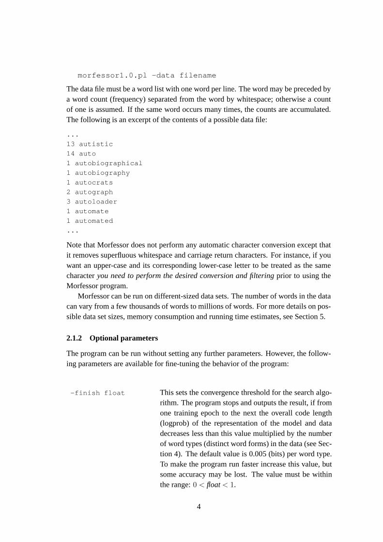
The data file must be a word list with one word per line. The word may be preceded bya word count (frequency) separated from the word by whitespace; otherwise a countof one is assumed. If the same word occurs many times, the counts are accumulated.The following is an excerpt of the contents of a possible data file:
...
13 autistic
14 auto
1 autobiographical
1 autobiography
1 autocrats
2 autograph
3 autoloader
1 automate
1 automated
...
Note that Morfessor does not perform any automatic character conversion except thatit removes superfluous whitespace and carriage return characters. For instance, if youwant an upper-case and its corresponding lower-case letter to be treated as the samecharacter you need to perform the desired conversion and filtering prior to using theMorfessor program.
Morfessor can be run on different-sized data sets. The number of words in the datacan vary from a few thousands of words to millions of words. For more details on pos-sible data set sizes, memory consumption and running time estimates, see Section 5.
2.1.2 Optional parameters
The program can be run without setting any further parameters. However, the follow-ing parameters are available for fine-tuning the behavior of the program:
-finish float This sets the convergence threshold for the search algo-rithm. The program stops and outputs the result, if fromone training epoch to the next the overall code length(logprob) of the representation of the model and datadecreases less than this value multiplied by the numberof word types (distinct word forms) in the data (see Sec-tion 4). The default value is 0.005 (bits) per word type.To make the program run faster increase this value, butsome accuracy may be lost. The value must be withinthe range: 0 < float < 1.
4
-rand integer This sets the random seed for the non-deterministicsearch algorithm (see Section 4). The default value iszero.
-savememory [int] This option can be used for reducing the memoryconsumption of the program (by approximately 25 %).When using the memory saving option every word inthe input data is not guaranteed to be processed in ev-ery training epoch. This leads to slower convergenceand longer (nearly doubled) processing time. The inte-ger parameter is a value that affects the randomness ofthe order in which words are processed. High values in-crease randomness, but may slow down the processing.The default value is 8. If the -savememory option isomitted, the memory saving feature is not used, whichis the best choice in most situations.
-gammalendistr
[float1 [float2]]
A gamma distribution is used for assigning prior prob-abilities to the lengths of morphs (see Section 3.5).Float1 corresponds to the most common morph lengthin the lexicon and float2 is the β parameter of the gammapdf (probability density function). The default valuesfor these parameters are 7.0 and 1.0, respectively. If thisoption is omitted, morphs in the lexicon are terminatedwith an end-of-morph character, which corresponds toan exponential pdf for morph lengths (for more detailsconsult Section 3.5).
-zipffreqdistr
[float]
A pdf derived from Mandelbrot’s correction of Zipf’slaw is used for assigning prior probabilities to the fre-quencies (number of occurrences) of the morphs. Thenumber (float) corresponds to the user’s belief of theproportion of hapax legomena, that is morphs that oc-cur only once in the morph segmentation of the words inthe data. The value must be within the range: 0 < float< 1. The default value is 0.5. If this option is omitted a(non-informative) morph frequency distribution derivedfrom combinatorics is used instead (consult Section 3.5for details).
5
-trace integer The progress of the processing is reported during the ex-ecution of the program. The integer consists of a sumof any or all of the following numbers, where the pres-ence of the number in the sum triggers the correspondingfunctionality:1: Flush output, i.e., do not buffer the the output stream,but output it right away.2: Output progress feedback (how many words pro-cessed etc.)4: Output each word when processed and its segmenta-tion.8: Trace recursive splitting of morphs.16: Upon termination output the length distribution ofthe morphs in the lexicon obtained.
2.1.3 Output
The Morfessor program writes its output to standard output. Some of the lines outputby the program are preceded by a number sign (#). These can be considered as “com-ments” and include, e.g., all information produced using the -trace option. Themain part of the output consists of the morph segmentations of the words in the input.The format used is exemplified by the following morph segmentations of some words.The words are preceded by their occurrence count (frequency) in the data:
...
13 autistic
14 auto
1 auto + biograph + ical
1 auto + biography
1 auto + crat + s
2 autograph
3 autoloader
1 automate
1 automate + d
...
The output can be directed to a file using the following syntax:
morfessor1.0.pl -data inputfilename > outputfilename
If additionally some optional parameters are defined, Morfessor can be invoked, e.g.,like this:
morfessor1.0.pl -savememory -gammalendistr 10 -trace 19
-data inputfilename > outputfilename
6
2.2 Using an existing model for segmenting new words
Once a morph segmentation model has been learned from some text data set, it canbe used for segmenting new word forms. In this segmentation mode of the Morfessorprogram no model learning takes place. Each input word is segmented into morphsby the Viterbi algorithm, which finds the most likely segmentation of the word intoa sequence of morphs that are present in the existing model. (In order to ensure thatthere is always at least one possible segmentation, every individual character in theword that does not already exist as a morph can be suggested as a morph with a verylow probability.)
In order to use an existing model for segmenting words, Morfessor is invoked asfollows:
morfessor1.0.pl -data filename1 -load filename2.
Filename1 is the input word list containing the word forms to be segmented. It hasexactly the same format as in Section 2.1.1 above. Filename2 refers to the segmen-tation model and is simply the output of an earlier run of the Morfessor program (seeSection 2.1.3 above).
No further parameters apply to the segmentation mode of the Morfessor program.The output is written to standard output and is of exactly the same format as in Sec-tion 2.1.3.
It may be of interest to some users that repeatedly running the same word listthrough the Morfessor program while always replacing filename2 with the most recentoutput corresponds to performing Expectation-Maximization (EM) using the Viterbialgorithm on the morph segmentations.
3 Mathematical formulation
The formulation of the Morfessor model is presented in a probabilistic framework, in-spired by the work of Brent (1999). Since the currently released Morfessor softwareonly implements the Morfessor Baseline models, which have been presented earlierin Creutz and Lagus (2002) and Creutz (2003), the following presentation only con-tains the mathematical formulation of these models variants. For the later Morfes-sor Category models the interested reader is referred to Creutz and Lagus (2004) andCreutz and Lagus (2005).
The mathematics of the original publications has undergone some modificationsin order to enable us to produce a unifying framework and in order to correct a fewinaccuracies. In addition, the Minimum Description Length (MDL) formulation inCreutz and Lagus (2002) has been replaced by a probabilistic maximum a posteriori(MAP) formulation in the current work. Conveniently, MDL and MAP are equivalentand produce the same result, as is demonstrated, e.g., by Chen (1996).
7
3.1 Maximum a posteriori estimate of the overall probability
The task is to induce a model of language in an unsupervised manner from a corpusof raw text. The model of language (M) consists of a morph vocabulary, or a lexi-con of morphs, and a grammar. We aim at finding the optimal model of language forproducing a segmentation of the corpus, i.e., a set of morphs that is concise, and more-over gives a concise representation for the corpus. The maximum a posteriori (MAP)estimate for the parameters, which is to be maximized, is:
arg maxM
P (M| corpus) = arg maxM
P (corpus |M) · P (M), where (1)
P (M) = P (lexicon, grammar). (2)
As can be seen above (Eq. 1), the MAP estimate consists of two parts: the probabilityof the model of language P (M) and the maximum likelihood (ML) estimate of thecorpus conditioned on the given model of language, written as P (corpus |M). Theprobability of the model of language (Eq. 2) is the joint probability of the probabilityof the induced lexicon and grammar. It incorporates our assumptions of how somefeatures should affect the morphology learning task. This is the Bayesian notion ofprobability, i.e., using probabilities for expressing degrees of prior belief rather thancounting relative frequency of occurrence in some empirical test setting.
In the following, we will describe the components of the Morfessor model ingreater detail, by studying the representation of the lexicon, grammar and corpus.
3.2 Lexicon
The lexicon contains one entry for each distinct morph (morph type) in the segmentedcorpus. We use the term “lexicon” to refer to an inventory of whatever information onemight want to store regarding a set of morphs, including their interrelations.
Suppose that the lexicon consists of M distinct morphs. The probability of comingup with a particular set of M morphs µ1 . . . µM making up the lexicon can be writtenas:
P (lexicon) = M ! · P (properties(µ1), . . . , properties(µM)). (3)
This indicates the joint probability that a set of morphs, each with a particular setof properties, is created. The factor M ! is explained by the fact that there are M !
possible orderings of a set of M items and the lexicon is the same regardless of theorder in which the M morphs emerged. (It is always possible to afterwards rearrangethe morphs into an unambiguously defined order, such as alphabetical order.)
In the Baseline versions of Morfessor, the only properties stored for a morph in thelexicon is the frequency (number of occurrences) of the morph in the corpus and thestring of letters that the morph consists of. The representation of the string of lettersnaturally incorporates knowledge about the length of the morph, i.e., the number ofletters in the string.
8
We assume that the frequency and morph string values are independent of eachother. Thus, we can write:
P (properties(µ1), . . . , properties(µM)) = P (fµ1, . . . , fµM
) · P (sµ1, . . . , sµM
), (4)
where f represents the morph frequency and s the morph string. Section 3.5 describesthe exact pdf:s (probability density functions) used for assigning probabilities to par-ticular morph strings and morph frequency values.
3.3 Grammar
Grammar can be viewed to contain information about how language units can be com-bined. In the later versions of Morfessor a simple morphotactics (word-internal syntax)is modeled. In the Baseline models, however, there is no context-sensitivity and thusno grammar to speak of. The probability P (lexicon, grammar) in Equation 2 reducesto P (lexicon). The lack of a grammar implies that a morph is as likely regardless ofwhich morphs precede or follow it or whether the morph is placed in the beginning,middle, or end of a word.
The probability of a morph µi is a maximum likelihood estimate. It is the frequencyof the morph in the corpus, fµi
, divided by the total number of morph tokens, N . Thevalue of N equals the sum of the frequency of each of the M morphs types:
P (µi) =fµi
N=
fµi∑M
j=1 fµj
. (5)
3.4 Corpus
Every word form in the corpus can be represented as a sequence of some morphs thatare present in the lexicon. Usually, there are many possible segmentations of a word.In MAP modeling, the one most probable segmentation is chosen. The probability ofthe corpus, when a particular model of language (lexicon and non-existent grammar)and morph segmentation is given, takes the form:
P (corpus |M) =W∏
j=1
nj∏
k=1
P (µjk). (6)
Products are taken over the W words in the corpus (token count), which are each splitinto nj morphs. The kth morph in the j th word, µjk, has the probability P (µjk), whichis calculated according to Eq. 5.
3.5 Properties of the morphs in the lexicon
A set of properties is stored for each morph in the lexicon, namely the frequency of themorph in the corpus and the string of letters the morph consists of. Each particular setof properties is assigned a probability according to given probability distributions.
9
The models presented in Creutz and Lagus (2002) and Creutz (2003) differ in theway they assign probabilities to different morph length and frequency values. Version1.0 of the Morfessor program supports both previous models, slightly modified. Whatwe here call the Morfessor Baseline model is based on Creutz and Lagus (2002) andwhat we call Morfessor Baseline-Freq-Length is based on Creutz (2003). Additionallythere are hybrids of the two, which we call Morfessor Baseline-Freq and MorfessorBaseline-Length.
The Baseline-Freq and Baseline-Freq-Length model variants differ from the othermodels in that an explicit prior probability distribution is used that affects the frequencydistribution of the morphs and that incorporates the user’s estimate of the proportionof hapax legomena, i.e., morph types that only occur once in the corpus.
The Baseline-Length and Baseline-Freq-Length model variants differ from the othermodels in that a prior probability distribution is used that affects the length distributionof the morphs and that incorporates the user’s estimate of the most common morphlength in the lexicon.
The pdf:s used for modeling morph frequency and morph length are describedbelow. For the Baseline model, Sections 3.5.1 and 3.5.3 apply. For the Baseline-Freqmodel, Sections 3.5.2 and 3.5.3 apply. For the Baseline-Length model, Sections 3.5.1and 3.5.4 apply, and for the Baseline-Freq-Length model, Sections 3.5.2 and 3.5.4apply.
3.5.1 Frequency modeled implicitly
By implicit modeling of morph frequency we mean that the user does not input his priorbelief of a desired morph frequency distribution. In this approach, we use one singleprobability for an entire morph frequency distribution. The value of P (fµ1
, . . . , fµM)
in Eq. 4 is then:
P (fµ1, . . . , fµM
) = 1/
(
N − 1
M − 1
)
=(M − 1)!(N −M)!
(N − 1)!, (7)
where N is the total number of morph tokens in the corpus, which equals the sum ofthe frequencies of the M morph types that make up the lexicon. The derivation ofthe formula can be found in Appendix A. This probability distribution corresponds toa non-informative prior in the sense that only the total number of morph tokens andtypes matter, not the individual morph frequencies.
3.5.2 Frequency modeled explicitly
By explicit modeling of morph frequency we mean that a probability distribution isused that assigns a particular probability to every possible morph frequency value.Here we assume that the frequency of one morph is independent of the frequencies of
10
1 2 3 4 5 6 7 8 9 100
0.1
0.2
0.3
0.4
0.5
Morph frequency
Prob
abili
tyZipf, power lawExponential
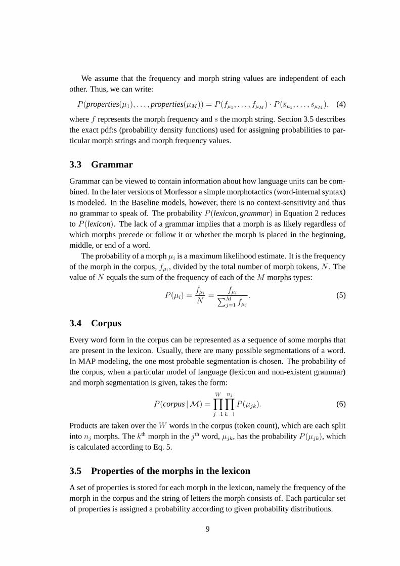
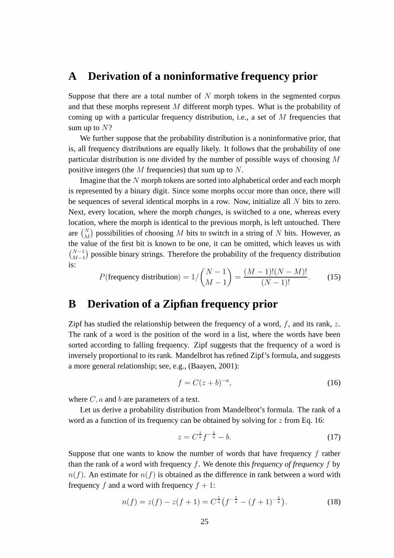
Figure 1. Probabilities ofmorph frequencies accordingto (1) a pdf derived fromMandelbrot’s correctionof Zipf’s law (h = 0.5)and (2) an approximatelyexponential pdf resultingfrom applying the non-informative frequency prior(N = 10 000, M = 5000).
the other morphs. Thus,
P (fµ1, . . . , fµM
) =
M∏
i=1
P (fµi). (8)
An expression for P (fµi) is derived in (Creutz, 2003) and it is based on Mandelbrot’s
correction of Zipf’s law. However, that derivation is unnecessarily complicated andincomplete. A better derivation is given in Appendix B and the result is:
P (fµi) = f log
2(1−h)
µi− (fµi
+ 1)log2(1−h). (9)
The parameter h represent the user’s prior belief of the proportion of hapax legomena,i.e., morph types that occur only once in the corpus. Typically, the proportion of hapaxlegomena is about half of all morph types.
In order to use this type of frequency prior in the Morfessor program, the-zipffreqprior switch must be activated. Optionally, a value for h can be en-tered. If omitted, a h value of 0.5 will be used by default. However, the difference ob-tained when using this Zipfian prior instead of the noninformative prior in Section 3.5.1is small.
Figure 1 illustrates the probability distributions obtained using the two approaches.The Zipfian prior corresponds to a power law curve. The non-informative prior ap-proximately results in an exponential distribution for the probability of the frequencyof an individual morph (see derivation in Appendix C). The curves are different, butnot radically different for small frequency values, which may explain why neither ap-proach performs significantly better than the other.
3.5.3 Length modeled implicitly
We make the simplifying assumption that the string that a morph consists of is inde-pendent of the strings that the other morphs consist of. Therefore, the joint probabilityP (sµ1
, . . . , sµM) in Eq. 4 reduces to the product of the probability of each individual
11
morph string:
P (sµ1, . . . , sµM
) =
M∏
i=1
P (sµi). (10)
We simplify further and assume that the letters in a morph string are drawn from aprobability distribution independently of each other. Thus, the probability of the stringof µi is the product of the probability of the individual letters, where cij represents thej th letter of the morph µi:
P (sµi) =
lµi∏
j=1
P (cij). (11)
The probability distribution over the alphabet P (cij) is estimated from the corpus bycomputing relative frequencies of each of the letters observed. The length of the stringis represented by lµi
.Now, implicit modeling of morph length implies that there is a special end-of-
morph character that is part of the alphabet and is appended to each morph string inthe lexicon and marks the end of the string. The probability that a morph of a particularlength l will emerge in this scheme is:
P (l) = [1− P (#)]l · P (#), (12)
where P (#) is the probability of the end-of-morph marker. The probability is theresult of first choosing l letters other than the end-of-morph marker and finally theend-of-morph marker. This is an exponential distribution, that is, the probability ofobserving a morph of a particular length decreases exponentially with the length of themorph.
3.5.4 Length modeled explicitly
Instead of using an end-of-morph marker for the morphs in the lexicon, one can firstdecide the length of the morph according to an appropriate probability distribution andthen choose the selected number of letters according to Eq. 11.
As a probability distribution for modeling morph length, a Poisson distributioncould be applied. Poisson distributions have been used for modeling word length, whenword tokens (words of running text) have been concerned, e.g., by Nagata (1997).However, here we model the length distribution of morph types (the morphs in thelexicon) and we have chosen to use a gamma distribution. This produces the followingformula for the prior probability of the morph length lµi
:
P (lµi) =
1
Γ(α)βαlµi
α−1e−lµi/β, (13)
where
Γ(α) =
∫
∞
0
zα−1e−zdz. (14)
12
1 3 5 7 9 11 13 15 17 190
0.05
0.1
0.15
0.2
Morph length
Prob
abili
tyFinnish
(a)
1 3 5 7 9 11 13 15 17 190
0.05
0.1
0.15
0.2
Morph length
Prob
abili
ty
English
Gold standardPoisson, best fitGamma, best fitGamma, actualExponential
(b)
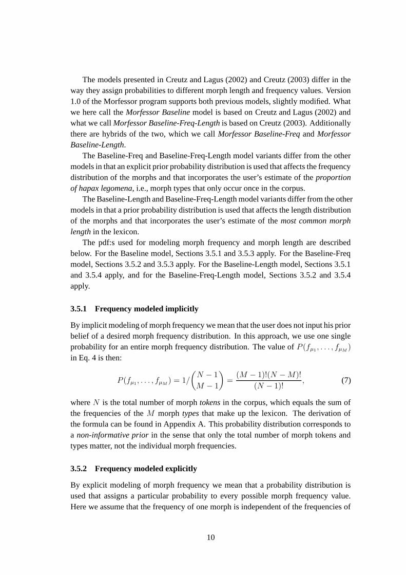
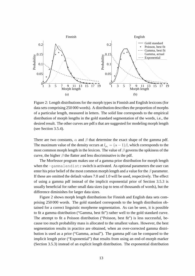
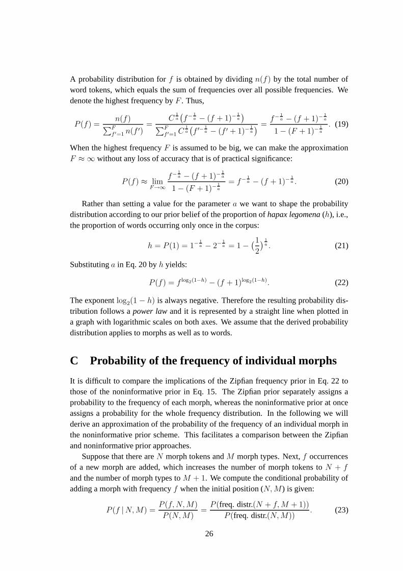
Figure 2: Length distributions for the morph types in Finnish and English lexicons (fordata sets comprising 250 000 words). A distribution describes the proportion of morphsof a particular length, measured in letters. The solid line corresponds to the empiricaldistribution of morph lengths in the gold standard segmentation of the words, i.e., thedesired result. The other curves are pdf:s that are suggested for modeling morph length(see Section 3.5.4).
There are two constants, α and β that determine the exact shape of the gamma pdf.The maximum value of the density occurs at lµi
= (α− 1)β, which corresponds to themost common morph length in the lexicon. The value of β governs the spikiness of thecurve, the higher β the flatter and less discriminative is the pdf.
The Morfessor program makes use of a gamma prior distribution for morph lengthwhen the -gammalendistr switch is activated. As optional parameters the user canenter his prior belief of the most common morph length and a value for the β parameter.If these are omitted the default values 7.0 and 1.0 will be used, respectively. The effectof using a gamma pdf instead of the implicit exponential prior of Section 3.5.3 isusually beneficial for rather small data sizes (up to tens of thousands of words), but thedifference diminishes for larger data sizes.
Figure 2 shows morph length distributions for Finnish and English data sets com-prising 250 000 words. The gold standard corresponds to the length distribution ob-tained for a correct linguistic morpheme segmentation. As can be seen, it is possibleto fit a gamma distribution (“Gamma, best fit”) rather well to the gold standard curve.The attempt to fit a Poisson distribution (“Poisson, best fit”) is less successful, be-cause too much probability mass is allocated to the smallest values. However, the bestsegmentation results in practice are obtained, when an over-corrected gamma distri-bution is used as a prior (“Gamma, actual”). The gamma pdf can be compared to theimplicit length prior (“Exponential”) that results from using an end-of-morph marker(Section 3.5.3) instead of an explicit length distribution. The exponential distribution
13
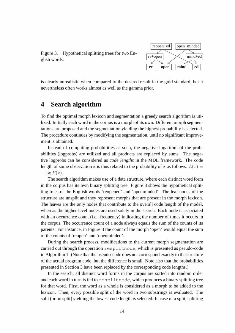
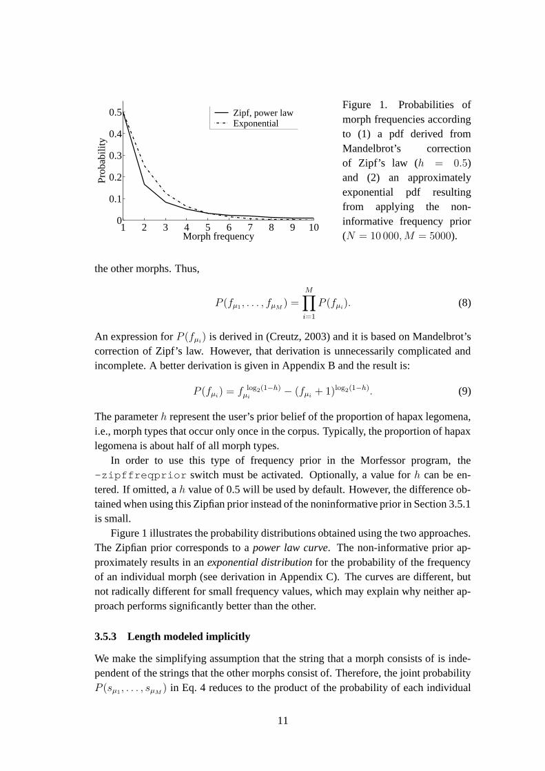
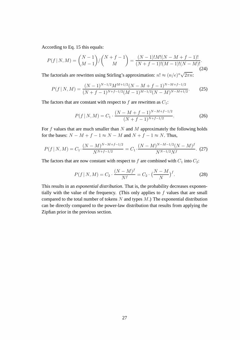
Figure 3. Hypothetical splitting trees for two En-glish words.
reopen+ed open+minded
re+open mind+ed
re open mind ed
is clearly unrealistic when compared to the desired result in the gold standard, but itnevertheless often works almost as well as the gamma prior.
4 Search algorithm
To find the optimal morph lexicon and segmentation a greedy search algorithm is uti-lized. Initially each word in the corpus is a morph of its own. Different morph segmen-tations are proposed and the segmentation yielding the highest probability is selected.The procedure continues by modifying the segmentation, until no significant improve-ment is obtained.
Instead of computing probabilities as such, the negative logarithm of the prob-abilities (logprobs) are utilized and all products are replaced by sums. The nega-tive logprobs can be considered as code lengths in the MDL framework. The codelength of some observation x is thus related to the probability of x as follows: L(x) =
− log P (x).The search algorithm makes use of a data structure, where each distinct word form
in the corpus has its own binary splitting tree. Figure 3 shows the hypothetical split-ting trees of the English words ‘reopened’ and ‘openminded’. The leaf nodes of thestructure are unsplit and they represent morphs that are present in the morph lexicon.The leaves are the only nodes that contribute to the overall code length of the model,whereas the higher-level nodes are used solely in the search. Each node is associatedwith an occurrence count (i.e., frequency) indicating the number of times it occurs inthe corpus. The occurrence count of a node always equals the sum of the counts of itsparents. For instance, in Figure 3 the count of the morph ‘open’ would equal the sumof the counts of ‘reopen’ and ‘openminded’.
During the search process, modifications to the current morph segmentation arecarried out through the operation resplitnode, which is presented as pseudo-codein Algorithm 1. (Note that the pseudo-code does not correspond exactly to the structureof the actual program code, but the difference is small. Note also that the probabilitiespresented in Section 3 have been replaced by the corresponding code lengths.)
In the search, all distinct word forms in the corpus are sorted into random orderand each word in turn is fed to resplitnode, which produces a binary splitting treefor that word. First, the word as a whole is considered as a morph to be added to thelexicon. Then, every possible split of the word in two substrings is evaluated. Thesplit (or no split) yielding the lowest code length is selected. In case of a split, splitting
14
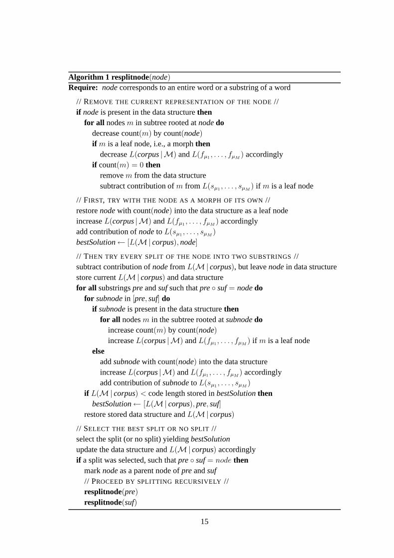
Algorithm 1 resplitnode(node)Require: node corresponds to an entire word or a substring of a word
// REMOVE THE CURRENT REPRESENTATION OF THE NODE //if node is present in the data structure then
for all nodes m in subtree rooted at node dodecrease count(m) by count(node)if m is a leaf node, i.e., a morph then
decrease L(corpus |M) and L(fµ1, . . . , fµM
) accordinglyif count(m) = 0 then
remove m from the data structuresubtract contribution of m from L(sµ1
, . . . , sµM) if m is a leaf node
// FIRST, TRY WITH THE NODE AS A MORPH OF ITS OWN //restore node with count(node) into the data structure as a leaf nodeincrease L(corpus |M) and L(fµ1
, . . . , fµM) accordingly
add contribution of node to L(sµ1, . . . , sµM
)
bestSolution← [L(M| corpus), node]
// THEN TRY EVERY SPLIT OF THE NODE INTO TWO SUBSTRINGS //subtract contribution of node from L(M| corpus), but leave node in data structurestore current L(M| corpus) and data structurefor all substrings pre and suf such that pre ◦ suf = node do
for subnode in [pre, suf] doif subnode is present in the data structure then
for all nodes m in the subtree rooted at subnode doincrease count(m) by count(node)increase L(corpus |M) and L(fµ1
, . . . , fµM) if m is a leaf node
elseadd subnode with count(node) into the data structureincrease L(corpus |M) and L(fµ1
, . . . , fµM) accordingly
add contribution of subnode to L(sµ1, . . . , sµM
)
if L(M| corpus) < code length stored in bestSolution thenbestSolution← [L(M| corpus), pre, suf]
restore stored data structure and L(M| corpus)
// SELECT THE BEST SPLIT OR NO SPLIT //select the split (or no split) yielding bestSolutionupdate the data structure and L(M| corpus) accordinglyif a split was selected, such that pre ◦ suf = node then
mark node as a parent node of pre and suf// PROCEED BY SPLITTING RECURSIVELY //resplitnode(pre)resplitnode(suf)
15
of the two parts continues recursively and stops when no more gains in overall codelength can be obtained by splitting a node into smaller parts. After all words have beenprocessed once, they are again shuffled by random, and each word is reprocessed usingresplitnode. This procedure is repeated until the overall code length of the modeland corpus does not decrease significantly from one epoch to the next. (The thresholdvalue for when to terminate the search can be set using the -finish switch in theMorfessor program. When the overall code length decreases less than the given valuefrom one epoch to the next, the search stops. The default threshold value is 0.005 bitsmultiplied by the number of word types in the corpus.)
Every word is processed once in every epoch, but due to the random shuffling, theorder in which the words are processed varies from one epoch to the next. It wouldbe possible to utilize a deterministic approach, where all words would be processed ina predefined order, but the stochastic approach (random shuffling) has been preferred,because we suspect that deterministic approaches might cause unforeseen bias. If onewere to employ a deterministic approach, it seems reasonable to sort the words in orderof increasing or decreasing length, but even so, words of the same length ought to beordered somehow, and for this purpose random shuffling seems much less prone tobias than, e.g., alphabetical ordering.
However, the stochastic nature of the algorithm means that the outcome dependson the series of random numbers produced by the random generator. The effect of thisindeterminism can be studied by running the Morfessor program on the same data, butusing different random seeds. The random seed is set using the -rand switch. Thedefault random seed is zero.
5 Experiments
We report the results of two experiments carried out on Finnish and English data setsof different sizes. In the first experiment (Section 5.2) we study the differences that areobtained if the Morfessor model is trained on a word token collection (a corpus, wherea word can occur many times) compared to a word type collection (a word list or acorpus vocabulary, where each distinct word form only occurs once). In the secondexperiment (Section 5.3) we study the effect of using the gamma length prior withdifferent amounts of data.
Additionally, we report the measured memory consumption and running times ofthe Morfessor program on a PC for some of the data sets (Section 5.4).
First, we briefly describe the data sets and evaluation measures used in the experi-ments.
16
5.1 Experimental setup
We are concerned with a linguistic morpheme segmentation task. The goal is to findthe locations of morpheme boundaries as accurately as possible. As a gold standard forthe desired locations of the morpheme boundaries, Hutmegs is used (see Section 5.1.2).Hutmegs consists of fairly accurate conventional linguistic morpheme segmentationsfor a large number of Finnish and English word forms.
5.1.1 Finnish and English data sets
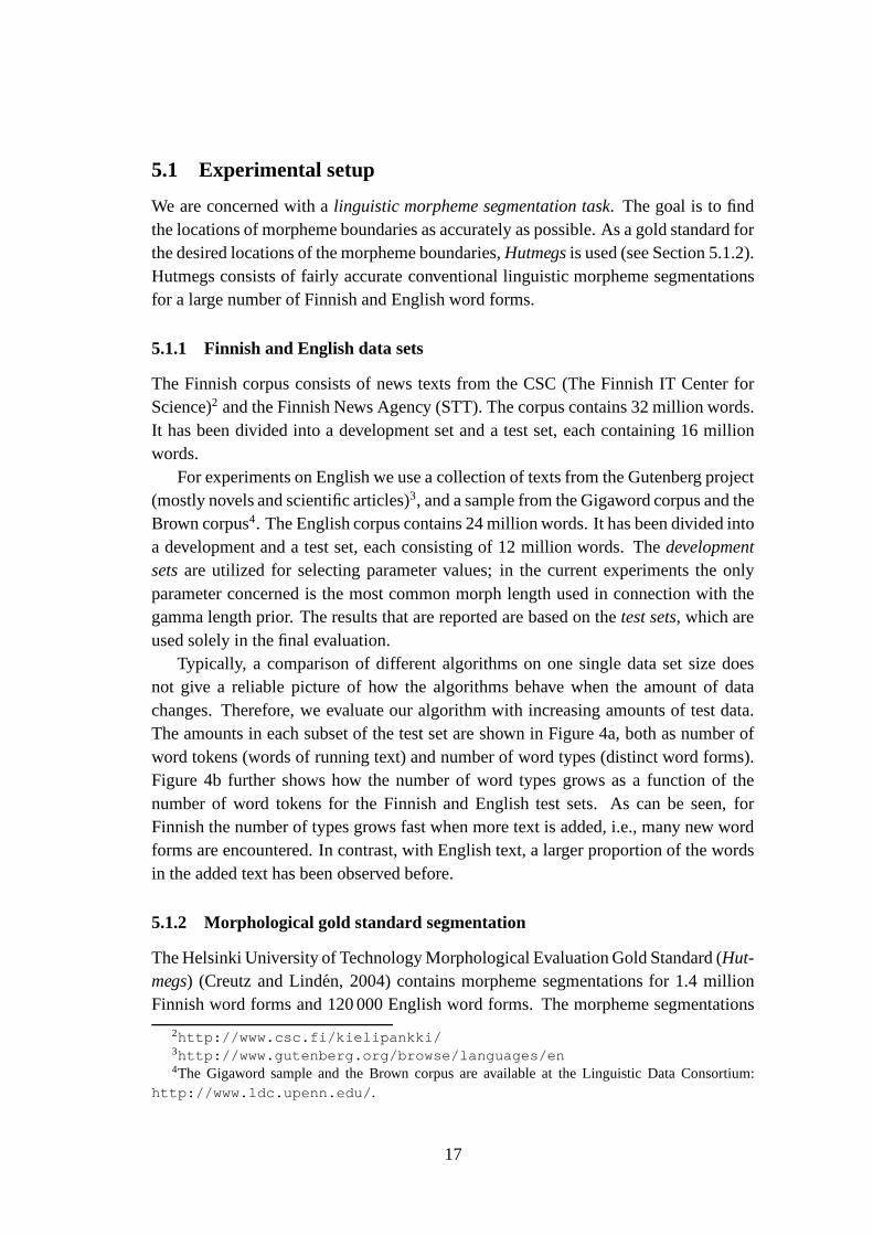
The Finnish corpus consists of news texts from the CSC (The Finnish IT Center forScience)2 and the Finnish News Agency (STT). The corpus contains 32 million words.It has been divided into a development set and a test set, each containing 16 millionwords.
For experiments on English we use a collection of texts from the Gutenberg project(mostly novels and scientific articles)3, and a sample from the Gigaword corpus and theBrown corpus4. The English corpus contains 24 million words. It has been divided intoa development and a test set, each consisting of 12 million words. The developmentsets are utilized for selecting parameter values; in the current experiments the onlyparameter concerned is the most common morph length used in connection with thegamma length prior. The results that are reported are based on the test sets, which areused solely in the final evaluation.
Typically, a comparison of different algorithms on one single data set size doesnot give a reliable picture of how the algorithms behave when the amount of datachanges. Therefore, we evaluate our algorithm with increasing amounts of test data.The amounts in each subset of the test set are shown in Figure 4a, both as number ofword tokens (words of running text) and number of word types (distinct word forms).Figure 4b further shows how the number of word types grows as a function of thenumber of word tokens for the Finnish and English test sets. As can be seen, forFinnish the number of types grows fast when more text is added, i.e., many new wordforms are encountered. In contrast, with English text, a larger proportion of the wordsin the added text has been observed before.
5.1.2 Morphological gold standard segmentation
The Helsinki University of Technology Morphological Evaluation Gold Standard (Hut-megs) (Creutz and Linden, 2004) contains morpheme segmentations for 1.4 millionFinnish word forms and 120 000 English word forms. The morpheme segmentations
2http://www.csc.fi/kielipankki/3http://www.gutenberg.org/browse/languages/en4The Gigaword sample and the Brown corpus are available at the Linguistic Data Consortium:
http://www.ldc.upenn.edu/.
17
Finnish Englishword tokens word types word types
10 000 5 500 2 40050 000 20 000 7 200
250 000 65 000 17 00012 000 000 – 110 00016 000 000 1 100 000 –
(a)
2 4 6 8 10 12 14
0.2
0.4
0.6
0.8
1
Tokens [million words]
Typ
es [
mill
ion
wor
ds]
Word tokens vs. word types
Finnish
English
(b)
Figure 4: (a) Sizes of the test data subsets used in the evaluation. (b) Curves of thenumber of word types observed for growing portions of the Finnish and English testsets.
have been produced semi-automatically using the two-level morphological analyzerFINTWOL for Finnish (Koskenniemi, 1983) and the CELEX database for English(Baayen et al., 1995). Both inflectional and derivational morphemes are marked in thegold standard. The Hutmegs package is publicly available on the Internet5. For full ac-cess to the Finnish morpheme segmentations, an inexpensive license must additionallybe purchased from Lingsoft, Inc.6 Similarly, the English CELEX database is requiredfor full access to the English material7.
As there can sometimes be many plausible segmentations of a word, Hutmegs pro-vides several alternatives when appropriate, e.g., English ‘evening’ (time of day) vs.‘even+ing’ (verb). There is also an option for so called “fuzzy” boundaries in theHutmegs annotations, which we have chosen to use. Fuzzy boundaries are applied incases where it is inconvenient to define one exact transition point between two mor-phemes. For instance, in English, the stem-final ‘e’ is dropped in some forms. Herewe allow two correct segmentations, namely the traditional linguistic segmentation in‘invite’, ‘invite+s’, ‘invit+ed’ and ‘invit+ing’, as well as the alternative interpretation,where the ‘e’ is considered part of the suffix, as in: ‘invit+e’, ‘invit+es’, ‘invit+ed’ and‘invit+ing’.
5http://www.cis.hut.fi/projects/morpho/6http://www.lingsoft.fi7The CELEX databases for English, Dutch and German are available at the Linguistic Data Consor-
tium: http://www.ldc.upenn.edu/.
18
5.1.3 Evaluation measures
As evaluation measures, we use precision and recall on discovered morpheme bound-aries. Precision is the proportion of correctly discovered boundaries among all dis-covered boundaries by the algorithm. Recall is the proportion of correctly discoveredboundaries among all correct boundaries. A high precision thus tells us that whena morpheme boundary is suggested, it is probably correct, but it does not tell us theproportion of missed boundaries. A high recall tells us that most of the desired bound-aries were indeed discovered, but it does not tell us how many incorrect boundarieswere suggested as well. In order to get a comprehensive idea of the performance of amethod, both measures must be taken into account.
The evaluation measures can be computed either using word tokens or word types.If the segmentation of word tokens is evaluated, frequent word forms will dominate inthe result, because every occurrence (of identical segmentations) of a word is included.If, instead, the segmentation of word types is evaluated, every distinct word form,frequent or rare, will have equal weight. When learning the morphology of a language,we consider all word forms to be as important regardless of their frequency. Therefore,in this paper, precision and recall for word types is reported.
For each of the data sizes 10 000, 50 000, and 250 000 words, the algorithms arerun on five separate subsets of the test data, and the average results are reported. Fur-thermore, statistical significance of the differences in performance have been assessedusing T-tests. The largest data sets, 16 million words (Finnish) and 12 million words(English) are exceptions, since they contain all available test data, which constrains thenumber of runs to one.
5.2 Learning a morph lexicon from word tokens vs. word types
Different morph segmentations are obtained if the algorithm is trained on a collectionof word tokens vs. word types. The former corresponds to a corpus, a piece of text,where words can occur many times. The latter corresponds to a corpus vocabulary,where only one occurrence of every distinct word form in the corpus has been listed.
We use the Morfessor Baseline model variant (see Section 3.5) to study how thesetwo different types of data lead to different morph segmentations. In the Baseline, noexplicit prior pdf:s are used for modeling morph frequency or length.
Figure 5 shows how precision and recall of segmentation develop for the two ap-proaches (word tokens vs. word types) with different amounts of data. The generaltrend for both languages is that when a larger data set is utilized, precision increaseswhile recall decreases. Furthermore, for every data size, learning from word typesleads to clearly higher recall and only slightly lower precision than learning from wordtokens8. Table 2 shows the segmentation of some words segmented by the Baseline
8According to T-tests the differences between measured precision and recall values are statistically
19
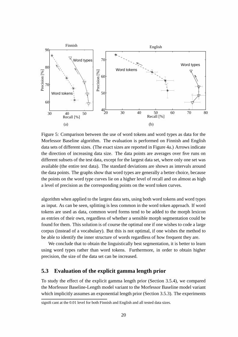
30 40 50
60
70
80
90
Recall [%]
Prec
isio
n [%
]Finnish
Word tokens
Word types
(a)
20 30 40 50 60 70 8040
50
60
70
Recall [%]
Prec
isio
n [%
]
English
Word tokensWord types
(b)
Figure 5: Comparison between the use of word tokens and word types as data for theMorfessor Baseline algorithm. The evaluation is performed on Finnish and Englishdata sets of different sizes. (The exact sizes are reported in Figure 4a.) Arrows indicatethe direction of increasing data size. The data points are averages over five runs ondifferent subsets of the test data, except for the largest data set, where only one set wasavailable (the entire test data). The standard deviations are shown as intervals aroundthe data points. The graphs show that word types are generally a better choice, becausethe points on the word type curves lie on a higher level of recall and on almost as higha level of precision as the corresponding points on the word token curves.
algorithm when applied to the largest data sets, using both word tokens and word typesas input. As can be seen, splitting is less common in the word token approach. If wordtokens are used as data, common word forms tend to be added to the morph lexiconas entries of their own, regardless of whether a sensible morph segmentation could befound for them. This solution is of course the optimal one if one wishes to code a largecorpus (instead of a vocabulary). But this is not optimal, if one wishes the method tobe able to identify the inner structure of words regardless of how frequent they are.
We conclude that to obtain the linguistically best segmentation, it is better to learnusing word types rather than word tokens. Furthermore, in order to obtain higherprecision, the size of the data set can be increased.
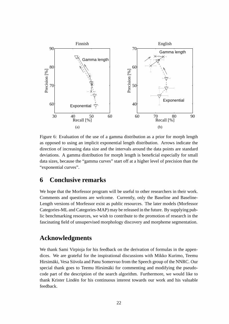
5.3 Evaluation of the explicit gamma length prior
To study the effect of the explicit gamma length prior (Section 3.5.4), we comparedthe Morfessor Baseline-Length model variant to the Morfessor Baseline model variantwhich implicitly assumes an exponential length prior (Section 3.5.3). The experiments
significant at the 0.01 level for both Finnish and English and all tested data sizes.
20
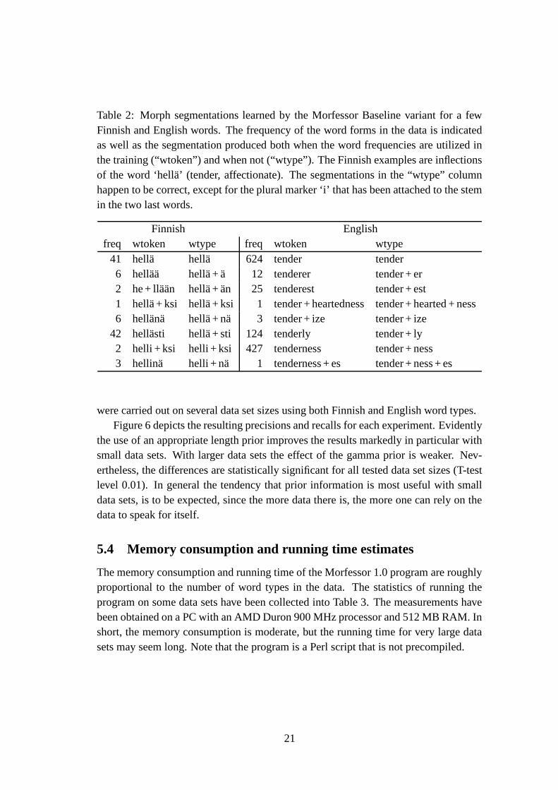
Table 2: Morph segmentations learned by the Morfessor Baseline variant for a fewFinnish and English words. The frequency of the word forms in the data is indicatedas well as the segmentation produced both when the word frequencies are utilized inthe training (“wtoken”) and when not (“wtype”). The Finnish examples are inflectionsof the word ‘hella’ (tender, affectionate). The segmentations in the “wtype” columnhappen to be correct, except for the plural marker ‘i’ that has been attached to the stemin the two last words.
Finnish Englishfreq wtoken wtype freq wtoken wtype
41 hella hella 624 tender tender6 hellaa hella + a 12 tenderer tender + er2 he + llaan hella + an 25 tenderest tender + est1 hella + ksi hella + ksi 1 tender + heartedness tender + hearted + ness6 hellana hella + na 3 tender + ize tender + ize
42 hellasti hella + sti 124 tenderly tender + ly2 helli + ksi helli + ksi 427 tenderness tender + ness3 hellina helli + na 1 tenderness + es tender + ness + es
were carried out on several data set sizes using both Finnish and English word types.Figure 6 depicts the resulting precisions and recalls for each experiment. Evidently
the use of an appropriate length prior improves the results markedly in particular withsmall data sets. With larger data sets the effect of the gamma prior is weaker. Nev-ertheless, the differences are statistically significant for all tested data set sizes (T-testlevel 0.01). In general the tendency that prior information is most useful with smalldata sets, is to be expected, since the more data there is, the more one can rely on thedata to speak for itself.
5.4 Memory consumption and running time estimates
The memory consumption and running time of the Morfessor 1.0 program are roughlyproportional to the number of word types in the data. The statistics of running theprogram on some data sets have been collected into Table 3. The measurements havebeen obtained on a PC with an AMD Duron 900 MHz processor and 512 MB RAM. Inshort, the memory consumption is moderate, but the running time for very large datasets may seem long. Note that the program is a Perl script that is not precompiled.
21
30 40 50 60
60
70
80
90
Recall [%]
Prec
isio
n [%
]Finnish
Exponential
Gamma length
(a)
60 70 80 90
40
50
60
70
Recall [%]
Prec
isio
n [%
]
English
Exponential
Gamma length
(b)
Figure 6: Evaluation of the use of a gamma distribution as a prior for morph lengthas opposed to using an implicit exponential length distribution. Arrows indicate thedirection of increasing data size and the intervals around the data points are standarddeviations. A gamma distribution for morph length is beneficial especially for smalldata sizes, because the “gamma curves” start off at a higher level of precision than the“exponential curves”.
6 Conclusive remarks
We hope that the Morfessor program will be useful to other researchers in their work.Comments and questions are welcome. Currently, only the Baseline and Baseline-Length versions of Morfessor exist as public resources. The later models (MorfessorCategories-ML and Categories-MAP) may be released in the future. By supplying pub-lic benchmarking resources, we wish to contribute to the promotion of research in thefascinating field of unsupervised morphology discovery and morpheme segmentation.
Acknowledgments
We thank Sami Virpioja for his feedback on the derivation of formulas in the appen-dices. We are grateful for the inspirational discussions with Mikko Kurimo, TeemuHirsimaki, Vesa Siivola and Panu Somervuo from the Speech group of the NNRC. Ourspecial thank goes to Teemu Hirsimaki for commenting and modifying the pseudo-code part of the description of the search algorithm. Furthermore, we would like tothank Krister Linden for his continuous interest towards our work and his valuablefeedback.
22
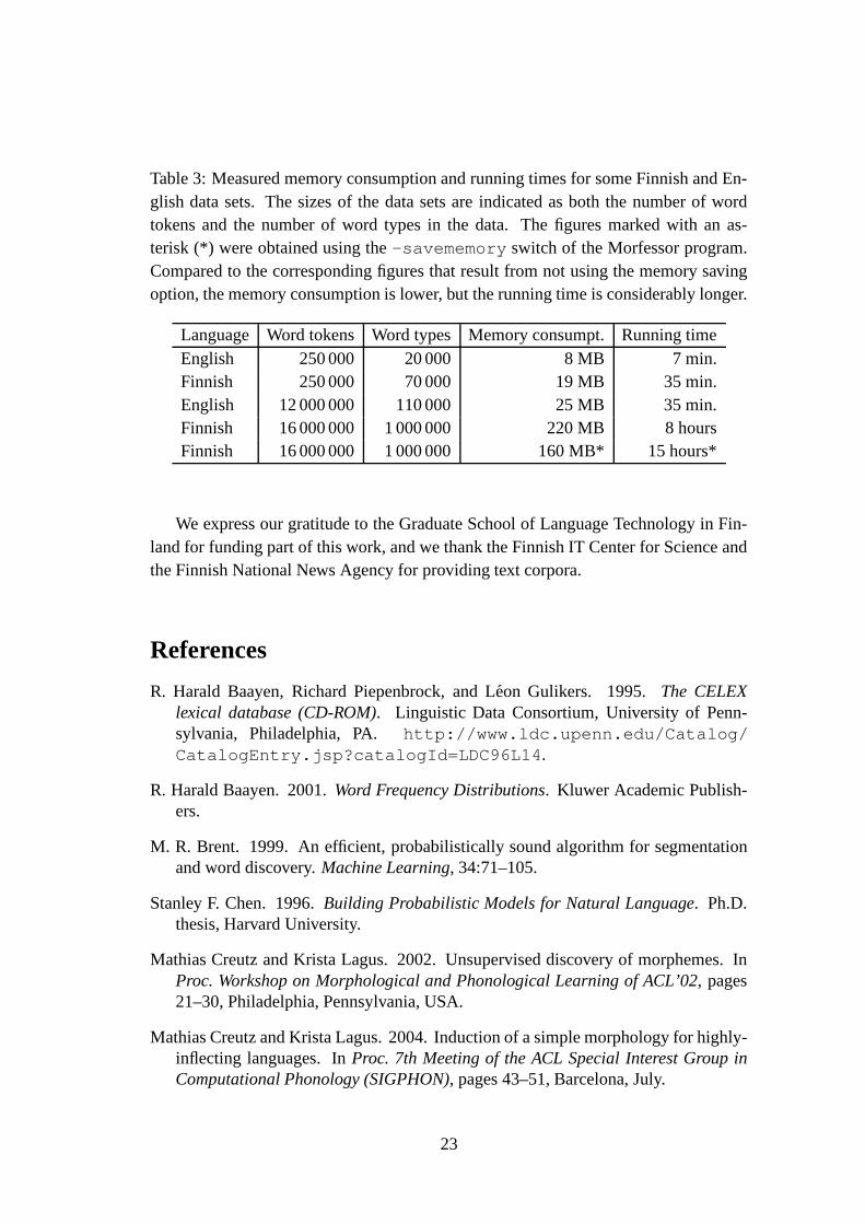
Table 3: Measured memory consumption and running times for some Finnish and En-glish data sets. The sizes of the data sets are indicated as both the number of wordtokens and the number of word types in the data. The figures marked with an as-terisk (*) were obtained using the -savememory switch of the Morfessor program.Compared to the corresponding figures that result from not using the memory savingoption, the memory consumption is lower, but the running time is considerably longer.
Language Word tokens Word types Memory consumpt. Running timeEnglish 250 000 20 000 8 MB 7 min.Finnish 250 000 70 000 19 MB 35 min.English 12 000 000 110 000 25 MB 35 min.Finnish 16 000 000 1 000 000 220 MB 8 hoursFinnish 16 000 000 1 000 000 160 MB* 15 hours*
We express our gratitude to the Graduate School of Language Technology in Fin-land for funding part of this work, and we thank the Finnish IT Center for Science andthe Finnish National News Agency for providing text corpora.
References
R. Harald Baayen, Richard Piepenbrock, and Leon Gulikers. 1995. The CELEXlexical database (CD-ROM). Linguistic Data Consortium, University of Penn-sylvania, Philadelphia, PA. http://www.ldc.upenn.edu/Catalog/CatalogEntry.jsp?catalogId=LDC96L14.
R. Harald Baayen. 2001. Word Frequency Distributions. Kluwer Academic Publish-ers.
M. R. Brent. 1999. An efficient, probabilistically sound algorithm for segmentationand word discovery. Machine Learning, 34:71–105.
Stanley F. Chen. 1996. Building Probabilistic Models for Natural Language. Ph.D.thesis, Harvard University.
Mathias Creutz and Krista Lagus. 2002. Unsupervised discovery of morphemes. InProc. Workshop on Morphological and Phonological Learning of ACL’02, pages21–30, Philadelphia, Pennsylvania, USA.
Mathias Creutz and Krista Lagus. 2004. Induction of a simple morphology for highly-inflecting languages. In Proc. 7th Meeting of the ACL Special Interest Group inComputational Phonology (SIGPHON), pages 43–51, Barcelona, July.
23
Mathias Creutz and Krista Lagus. 2005. Inducing the morphological lexicon of anatural language from unannotated text. In Proceedings of the International andInterdisciplinary Conference on Adaptive Knowledge Representation and Reason-ing (AKRR’05). (to appear).
Mathias Creutz and Krister Linden. 2004. Morpheme segmentation gold standardsfor Finnish and English. Technical Report A77, Publications in Computer andInformation Science, Helsinki University of Technology.
Mathias Creutz. 2003. Unsupervised segmentation of words using prior distributionsof morph length and frequency. In Proc. ACL’03, pages 280–287, Sapporo, Japan.
John Goldsmith. 2001. Unsupervised learning of the morphology of a natural lan-guage. Computational Linguistics, pages 27(2), 153–198.
K. Hacioglu, B. Pellom, T. Ciloglu, O. Ozturk, M. Kurimo, and M. Creutz. 2003. Onlexicon creation for Turkish LVCSR. In Proc. Eurospeech’03, pages 1165–1168,Geneva, Switzerland.
Kimmo Koskenniemi. 1983. Two-level morphology: A general computational modelfor word-form recognition and production. Ph.D. thesis, Two-level morphology:A general computational model for word-form recognition and production, Uni-versity of Helsinki.
Young-Suk Lee. 2004. Morphological analysis for statistical machine translation. InProc. Human Language Technology, Conference of the North American Chapter ofthe Association for Computational Linguistics, Boston, Massachusetts, USA.
Masaaki Nagata. 1997. A self-organizing Japanese word segmenter using heuristicword identification and re-estimation. In Proc. Fifth workshop on very large cor-pora, pages 203–215.
V. Siivola, T. Hirsimaki, M. Creutz, and M. Kurimo. 2003. Unlimited vocabularyspeech recognition based on morphs discovered in an unsupervised manner. InProc. Eurospeech’03, pages 2293–2296, Geneva, Switzerland.
24
A Derivation of a noninformative frequency prior
Suppose that there are a total number of N morph tokens in the segmented corpusand that these morphs represent M different morph types. What is the probability ofcoming up with a particular frequency distribution, i.e., a set of M frequencies thatsum up to N?
We further suppose that the probability distribution is a noninformative prior, thatis, all frequency distributions are equally likely. It follows that the probability of oneparticular distribution is one divided by the number of possible ways of choosing M
positive integers (the M frequencies) that sum up to N .Imagine that the N morph tokens are sorted into alphabetical order and each morph
is represented by a binary digit. Since some morphs occur more than once, there willbe sequences of several identical morphs in a row. Now, initialize all N bits to zero.Next, every location, where the morph changes, is switched to a one, whereas everylocation, where the morph is identical to the previous morph, is left untouched. Thereare
(
NM
)
possibilities of choosing M bits to switch in a string of N bits. However, asthe value of the first bit is known to be one, it can be omitted, which leaves us with(
N−1M−1
)
possible binary strings. Therefore the probability of the frequency distributionis:
P (frequency distribution) = 1/
(
N − 1
M − 1
)
=(M − 1)!(N −M)!
(N − 1)!. (15)
B Derivation of a Zipfian frequency prior
Zipf has studied the relationship between the frequency of a word, f , and its rank, z.The rank of a word is the position of the word in a list, where the words have beensorted according to falling frequency. Zipf suggests that the frequency of a word isinversely proportional to its rank. Mandelbrot has refined Zipf’s formula, and suggestsa more general relationship; see, e.g., (Baayen, 2001):
f = C(z + b)−a, (16)
where C, a and b are parameters of a text.Let us derive a probability distribution from Mandelbrot’s formula. The rank of a
word as a function of its frequency can be obtained by solving for z from Eq. 16:
z = C1
a f−1
a − b. (17)
Suppose that one wants to know the number of words that have frequency f ratherthan the rank of a word with frequency f . We denote this frequency of frequency f byn(f). An estimate for n(f) is obtained as the difference in rank between a word withfrequency f and a word with frequency f + 1:
n(f) = z(f)− z(f + 1) = C1
a
(
f−1
a − (f + 1)−1
a
)
. (18)
25
A probability distribution for f is obtained by dividing n(f) by the total number ofword tokens, which equals the sum of frequencies over all possible frequencies. Wedenote the highest frequency by F . Thus,
P (f) =n(f)
∑Ff ′=1 n(f ′)
=C
1
a
(
f−1
a − (f + 1)−1
a
)
∑Ff ′=1 C
1
a
(
f ′−1
a − (f ′ + 1)−1
a
)=
f−1
a − (f + 1)−1
a
1− (F + 1)−1
a
. (19)
When the highest frequency F is assumed to be big, we can make the approximationF ≈ ∞ without any loss of accuracy that is of practical significance:
P (f) ≈ limF→∞
f−1
a − (f + 1)−1
a
1− (F + 1)−1
a
= f−1
a − (f + 1)−1
a . (20)
Rather than setting a value for the parameter a we want to shape the probabilitydistribution according to our prior belief of the proportion of hapax legomena (h), i.e.,the proportion of words occurring only once in the corpus:
h = P (1) = 1−1
a − 2−1
a = 1−(1
2
)1
a . (21)
Substituting a in Eq. 20 by h yields:
P (f) = f log2(1−h) − (f + 1)log
2(1−h). (22)
The exponent log2(1 − h) is always negative. Therefore the resulting probability dis-tribution follows a power law and it is represented by a straight line when plotted ina graph with logarithmic scales on both axes. We assume that the derived probabilitydistribution applies to morphs as well as to words.
C Probability of the frequency of individual morphs
It is difficult to compare the implications of the Zipfian frequency prior in Eq. 22 tothose of the noninformative prior in Eq. 15. The Zipfian prior separately assigns aprobability to the frequency of each morph, whereas the noninformative prior at onceassigns a probability for the whole frequency distribution. In the following we willderive an approximation of the probability of the frequency of an individual morph inthe noninformative prior scheme. This facilitates a comparison between the Zipfianand noninformative prior approaches.
Suppose that there are N morph tokens and M morph types. Next, f occurrencesof a new morph are added, which increases the number of morph tokens to N + f
and the number of morph types to M + 1. We compute the conditional probability ofadding a morph with frequency f when the initial position (N, M ) is given:
P (f |N, M) =P (f, N, M)
P (N, M)=
P (freq. distr.(N + f, M + 1))
P (freq. distr.(N, M)). (23)
26
According to Eq. 15 this equals:
P (f |N, M) =
(
N − 1
M − 1
)
/
(
N + f − 1
M
)
=(N − 1)!M !(N −M + f − 1)!
(N + f − 1)!(M − 1)!(N −M)!.
(24)The factorials are rewritten using Stirling’s approximation: n! ≈ (n/e)n
√2πn:
P (f |N, M) =(N − 1)N−1/2MM+1/2(N −M + f − 1)N−M+f−1/2
(N + f − 1)N+f−1/2(M − 1)M−1/2(N −M)N−M+1/2. (25)
The factors that are constant with respect to f are rewritten as C1:
P (f |N, M) = C1 ·(N −M + f − 1)N−M+f−1/2
(N + f − 1)N+f−1/2. (26)
For f values that are much smaller than N and M approximately the following holdsfor the bases: N −M + f − 1 ≈ N −M and N + f − 1 ≈ N . Thus,
P (f |N, M) = C1 ·(N −M)N−M+f−1/2
NN+f−1/2= C1 ·
(N −M)N−M−1/2(N −M)f
NN−1/2Nf. (27)
The factors that are now constant with respect to f are combined with C1 into C2:
P (f |N, M) = C2 ·(N −M)f
Nf= C2 ·
(N −M
N
)f. (28)
This results in an exponential distribution. That is, the probability decreases exponen-tially with the value of the frequency. (This only applies to f values that are smallcompared to the total number of tokens N and types M .) The exponential distributioncan be directly compared to the power-law distribution that results from applying theZipfian prior in the previous section.
27