Evaluating Soil Liquefaction and Post-earthquake deformations using the CPT

P.K. Robertson University of Alberta, Dept. of Civil and Environmental Engineering, Edmonton, Canada

Keywords: Soil liquefaction, ground deformations, site investigation, cone penetration test.

ABSTRACT: Soil liquefaction is a major concern for many structures constructed with or on sand or sandy soils. This paper provides an overview of soil liquefaction, describes a method to evaluate the potential for cyclic liquefaction using the Cone Penetration Test (CPT) and methods to estimate post-earthquake ground deformations. A discussion is also provided on how to estimate the liquefied undrained shear strength fol-lowing strain softening (flow liquefaction).

1 INTRODUCTION

Soil liquefaction is a major concern for structures constructed with or on sand or sandy soils. The major earthquakes of Niigata in 1964 and Kobe in 1995 have illustrated the significance and extent of damage caused by soil liquefaction. Soil liquefac-tion is also a major design problem for large sand structures such as mine tailings impoundment and earth dams.

To evaluate the potential for soil liquefaction it is important to determine the soil stratigraphy and in-situ state of the deposits. The CPT is an ideal in-situ test to evaluate the potential for soil lique-faction because of its repeatability, reliability, con-tinuous data and cost effectiveness. This paper presents a summary of the application of the CPT to evaluate soil liquefaction. Further details are contained in a series of papers (Robertson and Wride, 1998; Youd et al., 2001; Zhang et al., 2002; Zhang et al., 2004).

2 DEFINITION OF SOIL LIQUEFACTION

Several phenomena are described as soil liquefac-tion, hence, a series of definitions are provided to aid in the understanding of the phenomena.

2.1 Cyclic (softening) Liquefaction • Requires undrained cyclic loading during

which shear stress reversal occurs or zero shear stress can develop.

• Requires sufficient undrained cyclic loading to allow effective stresses to reach essentially zero.

• Deformations during cyclic loading can accu-mulate to large values, but generally stabilize shortly after cyclic loading stops. The result-ing movements are due to external causes and occur mainly during the cyclic loading.

• Can occur in almost all saturated sandy soils provided that the cyclic loading is sufficiently large in magnitude and duration.

• Clayey soils generally do not experience cyclic liquefaction and deformations are generally small due to the cohesive nature of the soils. Rate effects (creep) often control deformations in cohesive soils.

2.2 Flow Liquefaction • Applies to strain softening soils only. • Requires a strain softening response in

undrained loading resulting in approximately constant shear stress and effective stress.

• Requires in-situ shear stresses to be greater than the residual or minimum undrained shear strength

• Either monotonic or cyclic loading can trigger flow liquefaction.

• For failure of a soil structure to occur, such as a slope, a sufficient volume of material must strain soften. The resulting failure can be a slide or a flow depending on the material char-acteristics and ground geometry. The resulting movements are due to internal causes and can occur after the trigger mechanism occurs.

• Can occur in any metastable saturated soil, such as very loose fine cohesionless deposits, very sensitive clays, and loess (silt) deposits.

Note that strain softening soils can also experi-

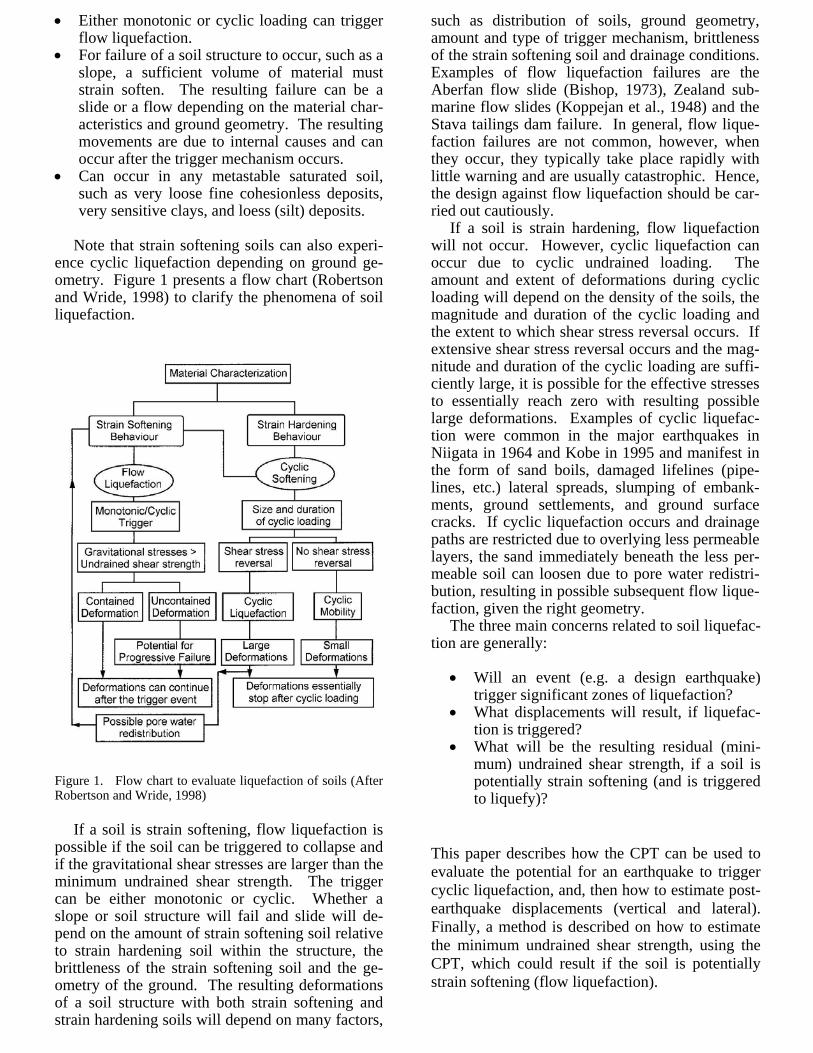
ence cyclic liquefaction depending on ground ge-ometry. Figure 1 presents a flow chart (Robertson and Wride, 1998) to clarify the phenomena of soil liquefaction.

Figure 1. Flow chart to evaluate liquefaction of soils (After Robertson and Wride, 1998)

If a soil is strain softening, flow liquefaction is possible if the soil can be triggered to collapse and if the gravitational shear stresses are larger than the minimum undrained shear strength. The trigger can be either monotonic or cyclic. Whether a slope or soil structure will fail and slide will de-pend on the amount of strain softening soil relative to strain hardening soil within the structure, the brittleness of the strain softening soil and the ge-ometry of the ground. The resulting deformations of a soil structure with both strain softening and strain hardening soils will depend on many factors,

such as distribution of soils, ground geometry, amount and type of trigger mechanism, brittleness of the strain softening soil and drainage conditions. Examples of flow liquefaction failures are the Aberfan flow slide (Bishop, 1973), Zealand sub-marine flow slides (Koppejan et al., 1948) and the Stava tailings dam failure. In general, flow lique-faction failures are not common, however, when they occur, they typically take place rapidly with little warning and are usually catastrophic. Hence, the design against flow liquefaction should be car-ried out cautiously.

If a soil is strain hardening, flow liquefaction will not occur. However, cyclic liquefaction can occur due to cyclic undrained loading. The amount and extent of deformations during cyclic loading will depend on the density of the soils, the magnitude and duration of the cyclic loading and the extent to which shear stress reversal occurs. If extensive shear stress reversal occurs and the mag-nitude and duration of the cyclic loading are suffi-ciently large, it is possible for the effective stresses to essentially reach zero with resulting possible large deformations. Examples of cyclic liquefac-tion were common in the major earthquakes in Niigata in 1964 and Kobe in 1995 and manifest in the form of sand boils, damaged lifelines (pipe-lines, etc.) lateral spreads, slumping of embank-ments, ground settlements, and ground surface cracks. If cyclic liquefaction occurs and drainage paths are restricted due to overlying less permeable layers, the sand immediately beneath the less per-meable soil can loosen due to pore water redistri-bution, resulting in possible subsequent flow lique-faction, given the right geometry.

The three main concerns related to soil liquefac-tion are generally:

• Will an event (e.g. a design earthquake)

trigger significant zones of liquefaction? • What displacements will result, if liquefac-

tion is triggered? • What will be the resulting residual (mini-

mum) undrained shear strength, if a soil is potentially strain softening (and is triggered to liquefy)?

This paper describes how the CPT can be used to evaluate the potential for an earthquake to trigger cyclic liquefaction, and, then how to estimate post-earthquake displacements (vertical and lateral). Finally, a method is described on how to estimate the minimum undrained shear strength, using the CPT, which could result if the soil is potentially strain softening (flow liquefaction).

3 CYCLIC LIQUEFACTION

Most of the existing work on cyclic liquefaction has been primarily for earthquakes. The late Prof. H.B. Seed and his co-workers developed a com-prehensive methodology to estimate the potential for cyclic liquefaction due to earthquake loading. The methodology requires an estimate of the cyclic stress ratio (CSR) profile caused by the design earthquake and the cyclic resistance ratio (CRR) of the ground. If the CSR is greater than the CRR cyclic liquefaction can occur. The CSR is usually estimated based on a probability of occurrence for a given earthquake. A site-specific seismicity analysis can be carried out to determine the design CSR profile with depth. A simplified method to estimate CSR was also developed by Seed and Idriss (1971) based on the maximum ground sur-face acceleration (amax) at the site. The simplified approach can be summarized as follows:

CSR = dvo

vomax

vo

av r'g

a65.0

' ⎟⎟⎠

⎞⎜⎜⎝

⎛σσ

⎥⎦

⎤⎢⎣

⎡=

στ

[1]

Where τav is the average cyclic shear stress; amax

is the maximum horizontal acceleration at the ground surface; g = 9.81m/s2 is the acceleration due to gravity; σvo and σ'vo are the total and effec-tive vertical overburden stresses, respectively; and rd is a stress reduction factor which is dependent on depth. The factor rd can be estimating using the following bi-linear function, which provides a good fit to the average of the suggested range in rd originally proposed by Seed and Idriss (1971):

rd = 1.0 – 0.00765z [2]

if z < 9.15 m

= 1.174 – 0.0267z

if z = 9.15 to 23 m Where z is the depth in metres. These formulae

are approximate at best and represent only average values since rd shows considerable variation with depth.

Seed et al., (1985) also developed a method to

estimate the cyclic resistance ratio (CRR) for clean sand with level ground conditions based on the Standard Penetration Test (SPT). Recently the CPT has become more popular to estimate CRR, due to the continuous, reliable and repeatable na-ture of the data (Youd et al., 2001).

In recent years, there has been an increase in available field performance data, especially for the CPT (Robertson and Wride, 1998). The recent field performance data have shown that the exist-ing CPT-based correlation by Robertson and Cam-panella (1985) for clean sands is generally good. Based on discussions at the 1996 NCEER work-shop (NCEER, 1997), the curve by Robertson and Campanella (1985) has been adjusted slightly at the lower end. The resulting recommended CPT correlation for clean sand is shown in Figure 2 and can be estimated using the following simplified equations:

CRR7.5 = ( )

08.01000q

933

csN1c +⎥⎦

⎤⎢⎣

⎡ [3]

if 50 ≤ (qc1N)cs ≤ 160

CRR7.5 = ( )

05.01000

833.0 1 +⎥⎦

⎤⎢⎣

⎡ csNcq

if (qc1N)cs < 50

Figure 2. Cyclic resistance ratio (CRR) from the CPT for clean sands. (After Robertson and Wride, 1998).

Where (qc1N)cs is the equivalent clean sand nor-malized cone penetration resistance (defined in de-tail later).

The field observations used to compile the curve in Figure 2 are based primarily on the fol-lowing conditions:

• Holocene age, clean sand deposits • Level or gently sloping ground • Magnitude M = 7.5 earthquakes • Depth range from 1 to 15 m (85% is for depths

< 10 m) • Representative average CPT values for the

layer considered to have experienced cyclic liquefaction.

Caution should be exercised when extrapolating

the CPT correlation to conditions outside the above range. An important feature to recognize is that the correlation is based primarily on average val-ues for the inferred liquefied layers. However, the correlation is often applied to all measured CPT values, which include low values below the aver-age. Therefore, the correlation can be conservative in variable deposits where a small part of the CPT data can indicate possible liquefaction.

It has been recognized for some time that the correlation to estimate CRR7.5 for silty sands is dif-ferent than that for clean sands. Typically a cor-rection is made to determine an equivalent clean sand penetration resistance based on grain charac-teristics, such as fines content, although the correc-tions are due to more than just fines content, since the plasticity of the fines also has an influence on the CRR.

One reason for the continued use of the SPT has been the need to obtain a soil sample to determine the fines content of the soil. However, this has been offset by the generally poor repeatability and reliability of the SPT data. It is now possible to es-timate grain characteristics directly from the CPT. Robertson and Wride (1998) suggest estimating an equivalent clean sand normalized cone penetration resistance, (qc1N)cs using the following:

(qc1N)cs = Kc (qc1N) [4] where Kc is a correction factor that is a function

of grain characteristics of the soil. Robertson and Wride (1998) suggest estimating

the grain characteristics using the soil behavior chart by Robertson (1990) (see Figure 3) and the soil behavior type index, Ic, where;

Ic = [5] ( ) ([ 5.022 22.1FlogQlog47.3 ++− ) ]

where Q = qc1N = n

vo

a

2a

voc

'P

Pq

⎟⎟⎠

⎞⎜⎜⎝

⎛σ⎟⎟

⎠

⎞⎜⎜⎝

⎛ σ−

is the normalized CPT penetration resistance, di-mensionless; n = stress exponent; F = fs/[(qc - σvo)] x 100% is the normalized friction ratio, in percent; fs is the CPT sleeve friction stress; σvo and σ'vo are the total effective overburden stresses, respec-tively; Pa is a reference pressure in the same units as σ'vo (i.e. Pa = 100 kPa if σ'vo is in kPa); and Pa2 is a reference pressure in the same units as qc and σvo (i.e. Pa2 = 0.1 MPa if qc and σvo are in MPa). Robertson and Wride (1998) used a form of qc1N that did not subtract the total vertical stress (σvo) from qc and used n = 0.5. The more correct ap-proach is the full form shown in equation 5. In general there is little difference between qc1N and Q for most sandy soils at shallow depth (σ'vo < 300 kPa).

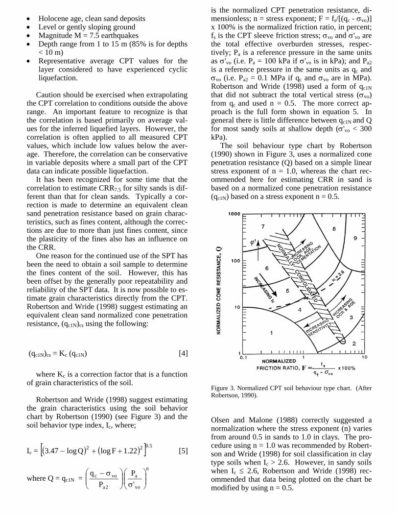
The soil behaviour type chart by Robertson (1990) shown in Figure 3, uses a normalized cone penetration resistance (Q) based on a simple linear stress exponent of n = 1.0, whereas the chart rec-ommended here for estimating CRR in sand is based on a normalized cone penetration resistance (qc1N) based on a stress exponent n = 0.5.

Figure 3. Normalized CPT soil behaviour type chart. (After Robertson, 1990).

Olsen and Malone (1988) correctly suggested a normalization where the stress exponent (n) varies from around 0.5 in sands to 1.0 in clays. The pro-cedure using n = 1.0 was recommended by Robert-son and Wride (1998) for soil classification in clay type soils when Ic > 2.6. However, in sandy soils when Ic ≤ 2.6, Robertson and Wride (1998) rec-ommended that data being plotted on the chart be modified by using n = 0.5.

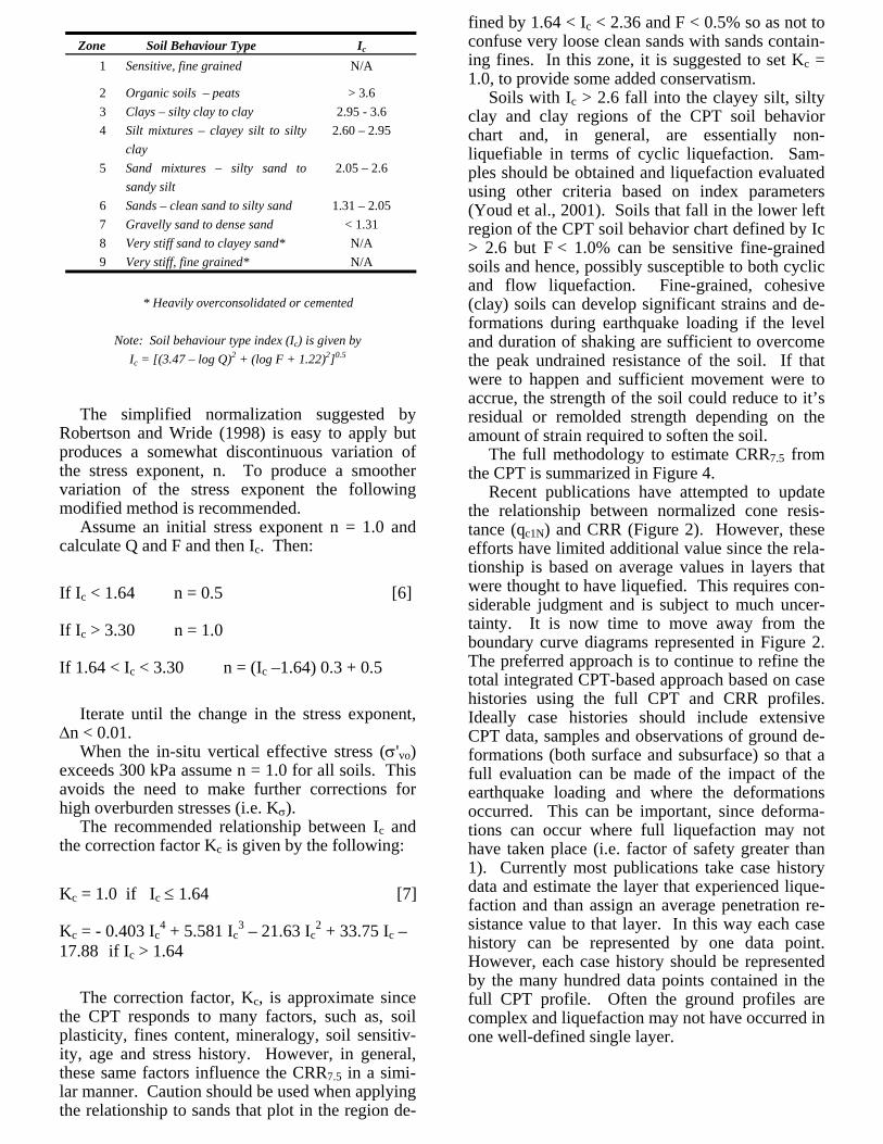
Zone Soil Behaviour Type Ic

1 Sensitive, fine grained N/A

2 Organic soils – peats > 3.6 3 Clays – silty clay to clay 2.95 - 3.6 4 Silt mixtures – clayey silt to silty

clay 2.60 – 2.95

5 Sand mixtures – silty sand to sandy silt

2.05 – 2.6

6 Sands – clean sand to silty sand 1.31 – 2.05 7 Gravelly sand to dense sand < 1.31 8 Very stiff sand to clayey sand* N/A 9 Very stiff, fine grained* N/A

* Heavily overconsolidated or cemented

Note: Soil behaviour type index (Ic) is given by

Ic = [(3.47 – log Q)2 + (log F + 1.22)2]0.5

The simplified normalization suggested by Robertson and Wride (1998) is easy to apply but produces a somewhat discontinuous variation of the stress exponent, n. To produce a smoother variation of the stress exponent the following modified method is recommended.

Assume an initial stress exponent n = 1.0 and calculate Q and F and then Ic. Then:

If Ic < 1.64 n = 0.5 [6]

If Ic > 3.30 n = 1.0

If 1.64 < Ic < 3.30 n = (Ic –1.64) 0.3 + 0.5 Iterate until the change in the stress exponent,

∆n < 0.01. When the in-situ vertical effective stress (σ'vo)

exceeds 300 kPa assume n = 1.0 for all soils. This avoids the need to make further corrections for high overburden stresses (i.e. Kσ).

The recommended relationship between Ic and the correction factor Kc is given by the following:

Kc = 1.0 if Ic ≤ 1.64 [7]

Kc = - 0.403 Ic4 + 5.581 Ic

3 – 21.63 Ic2 + 33.75 Ic –

17.88 if Ic > 1.64 The correction factor, Kc, is approximate since

the CPT responds to many factors, such as, soil plasticity, fines content, mineralogy, soil sensitiv-ity, age and stress history. However, in general, these same factors influence the CRR7.5 in a simi-lar manner. Caution should be used when applying the relationship to sands that plot in the region de-

fined by 1.64 < Ic < 2.36 and F < 0.5% so as not to confuse very loose clean sands with sands contain-ing fines. In this zone, it is suggested to set Kc = 1.0, to provide some added conservatism.

Soils with Ic > 2.6 fall into the clayey silt, silty clay and clay regions of the CPT soil behavior chart and, in general, are essentially non-liquefiable in terms of cyclic liquefaction. Sam-ples should be obtained and liquefaction evaluated using other criteria based on index parameters (Youd et al., 2001). Soils that fall in the lower left region of the CPT soil behavior chart defined by Ic > 2.6 but F < 1.0% can be sensitive fine-grained soils and hence, possibly susceptible to both cyclic and flow liquefaction. Fine-grained, cohesive (clay) soils can develop significant strains and de-formations during earthquake loading if the level and duration of shaking are sufficient to overcome the peak undrained resistance of the soil. If that were to happen and sufficient movement were to accrue, the strength of the soil could reduce to it’s residual or remolded strength depending on the amount of strain required to soften the soil.

The full methodology to estimate CRR7.5 from the CPT is summarized in Figure 4.

Recent publications have attempted to update the relationship between normalized cone resis-tance (qc1N) and CRR (Figure 2). However, these efforts have limited additional value since the rela-tionship is based on average values in layers that were thought to have liquefied. This requires con-siderable judgment and is subject to much uncer-tainty. It is now time to move away from the boundary curve diagrams represented in Figure 2. The preferred approach is to continue to refine the total integrated CPT-based approach based on case histories using the full CPT and CRR profiles. Ideally case histories should include extensive CPT data, samples and observations of ground de-formations (both surface and subsurface) so that a full evaluation can be made of the impact of the earthquake loading and where the deformations occurred. This can be important, since deforma-tions can occur where full liquefaction may not have taken place (i.e. factor of safety greater than 1). Currently most publications take case history data and estimate the layer that experienced lique-faction and than assign an average penetration re-sistance value to that layer. In this way each case history can be represented by one data point. However, each case history should be represented by the many hundred data points contained in the full CPT profile. Often the ground profiles are complex and liquefaction may not have occurred in one well-defined single layer.

if Ic <= 1.64, Kc = 1.0if 1.64< Ic < 2.60, Kc = -0.403I c

4 + 5.581 I c3 – 21.63 I c

2 + 33.75 Ic – 17.88if Ic >= 2.60, evaluate using other criteria; likely non- liquefiable if F > 1%

BUT, if 1.64 < Ic < 2.36 and F < 0.5%, set Kc = 1.0

08.01000

)(933

15.7 +

⎠⎞

⎜⎝⎛⋅= csNcqCRR , if 50 <= (q c1N )cs < 160

05.01000

)(833.0 15.7 +

⎠⎞

⎜⎝⎛⋅= csNcqCRR , if (q c1N )cs < 50

if Ic >= 2.60, evaluate using other criteria; likely non- liquefiable if F > 1%

QKq ccsNc ⋅=)( 1

qc : tip resistance, fs : sleeve frictionσvo , σvo’ : in-situ vertical total and effective stress

units: all in kPa

initial stress exponent : n = 1.0 and calcualte Q, F, and Ic

if Ic <= 1.64, n = 0.5if 1.64 < Ic < 3.30, n = ( Ic –1.64)*0.3 + 0.5

if Ic >= 3.30, n = 1.0iterate until the change in n, ∆n < 0.01

if σvo’ > 300 kPa, let n = 1.0 for all soils

n

vonC

⎠

⎞⎜⎜⎝

⎛=

'100σ

nvoc CqQ ⋅

−=

100)( σ

, 100)(

⋅−

=voc

s

qfFσ

[ ]22 )log22.1()log47.3( FQI c ++−=

Liquefaction often occurs in multiple layers, which can only be observed in the full CPT profile. It can be overly simplistic to represent a complex ground profile and case history by one data point on a boundary curve like Figure 2. These curves have served as an excellent starting point in the development of the current simplified CPT and SPT liquefaction methods now available, however, it is now time to leave these highly simplistic curves and progress using data captured in the full soil profile.

The factor of safely against liquefaction is de-fined as:

Factor of Safety, FS = CSR

CRR 5.7 MSF [8]

where MSF is the Magnitude Scaling Factor to

convert the CRR7.5 for M = 7.5 to the equivalent CRR for the design earthquake. The recom-mended MSF is given by:

MSF = 56.2M174 [9]

The above recommendations are based on the

NCEER Workshop in 1996 (Youd et al., 2001).

An example of the CPT method to evaluate cy-clic liquefaction is shown on Figure 5 for the Moss Landing site that suffered cyclic liquefaction dur-ing the 1989 Loma Prieta earthquake in California (Boulanger et al., 1997).

Figure 4. Flow chart to evaluate cyclic resistance ratio (CRR) from the CPT. (Modified from Robertson and Wride, 1998).

Figure 5. Example of CPT to evaluate cyclic liquefaction at Moss Landing Site. (After Robertson and Wride, 1998).

A major advantage of the CPT approach is the continuous and reliable nature of the data. CPT data are typically collected every 5 cm (2 inches). This means that data points are collected at the in-terface between layers, such as between clay and sand. During this transition, the CPT data points do not accurately capture the correct soil response since the penetration resistance is moving from ei-ther low to high values or vis-a-versa. The CPT penetration resistance represents an average re-sponse of the ground within a sphere of influence that can vary from a few cone diameters in soft clay to 20 cone diameters in dense sand. In these thin transition zones the CPT-based liquefaction method can predict low values of CRR. This is il-lustrated in Figure 5 at depths of around 6m and 10m, where there are clear interface boundaries be-tween sand and clay. At these locations there a few data points that indicate low values of CRR and hence liquefaction. These thin interface zones are easy to identify and account for in the interpre-tation. In the following sections, methods to esti-mate post-earthquake ground deformations will be presented and discussed. Using these CPT-based methods, it is simple to identify the thin interface transition zones and remove, where appropriate.

A key advantage of the CPT based liquefaction method is that continuous profiles can be calcu-lated quickly, which allows the engineer time to study the profile in detail and apply engineering judgment where appropriate. The CPT-based liq-uefaction method is a simplified approach and is hence conservative. The method was developed from the limit boundary curve in Figure 2 that was developed using average values but the resulting method is applied using all data points. Also, the continuous CPT data predicts low values of CRR in the thin interface transitions zones, as described above.

Juang et al. (1999) has shown that the Robert-son and Wride CPT-based liquefaction method has the same level of conservatism as the Seed et al SPT-based liquefaction method, both represent a probability of liquefaction of between 20% to 30% (i.e. more conservative than the expected 50% probability). This conclusion was supported by the NCEER workshop (Youd et al., 2001).

4 POST-EARTHQUAKE DEFORMATIONS

The CPT-based method described above, can pro-vide continuous profiles of CRR and Factor of Safety for given design earthquake loading. How-ever, Factor of Safety is not always the most mean-

ingful means to evaluate liquefaction potential. For most projects a more meaningful evaluation of the effect of a design earthquake on a given project is to estimate the ground deformations that may re-sult from the earthquake. Ground deformations that follow earthquake loading are either vertical settlements or lateral deformations. Although the Factor of Safety due to a design earthquake may be less than 1.0, the resulting deformations may be ei-ther acceptable for the project or can be accommo-dated with appropriate design of the structures.

5 LIQUEFACTION INDUCED VERTICAL GROUND SETTLEMENTS

Liquefaction-induced ground settlements are es-sentially vertical deformations of surficial soil lay-ers caused by the densification and compaction of loose granular soils following earthquake loading. Several methods have been proposed to calculate liquefaction-induced ground deformations, includ-ing numerical and analytical methods, laboratory modeling and testing, and field-testing-based methods. The expense and difficulty associated with obtaining and testing high quality samples of loose sandy soils may only be feasible for high-risk projects where the consequences of liquefac-tion may result in severe damage and large costs. Semi-empirical approaches using data from field tests are likely best suited to provide simple, reli-able and direct methods to estimate liquefaction-induced ground deformations for low to medium risk projects, and also to provide preliminary esti-mates for higher risk projects. Zhang et al. (2002) proposed a simple semi-empirical method using the CPT to estimate liquefaction induced ground settlements for level ground.

For sites with level ground, far from any free face (e.g., river banks, seawalls), it is reasonable to assume that little or no lateral displacement occurs after the earthquake, such that the volumetric strain will be equal or close to the vertical strain. If the vertical strain in each soil layer is integrated with depth using Equation [10], the result should be an appropriate index of potential liquefaction-induced ground settlement at the CPT location due to the design earthquake,

∑=

∆=j

iiiv zS

1

ε [10]

Where: S is the calculated liquefaction-induced ground settlement at the CPT location; εvi is the post-liquefaction volumetric strain for the soil sub-layer i; ∆zi is the thickness of the sub-layer i; and j is the number of soil sub-layers.

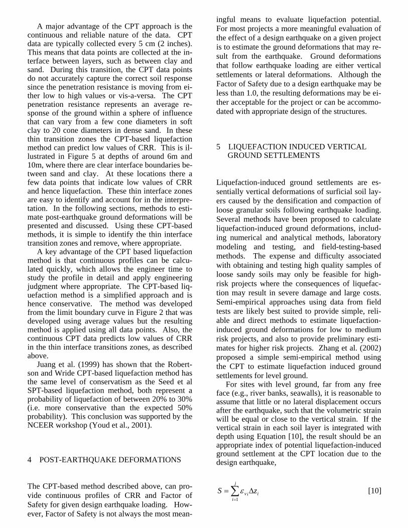
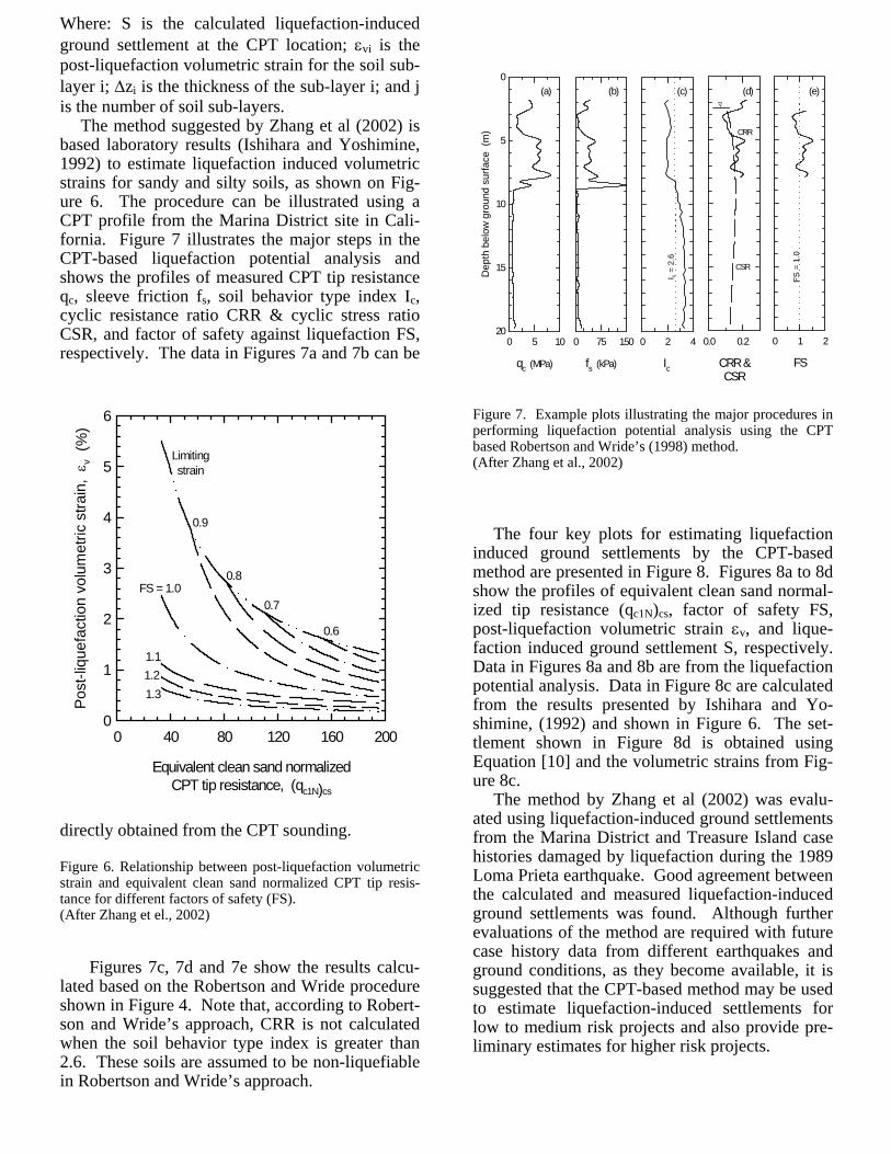
The method suggested by Zhang et al (2002) is based laboratory results (Ishihara and Yoshimine, 1992) to estimate liquefaction induced volumetric strains for sandy and silty soils, as shown on Fig-ure 6. The procedure can be illustrated using a CPT profile from the Marina District site in Cali-fornia. Figure 7 illustrates the major steps in the CPT-based liquefaction potential analysis and shows the profiles of measured CPT tip resistance qc, sleeve friction fs, soil behavior type index Ic, cyclic resistance ratio CRR & cyclic stress ratio CSR, and factor of safety against liquefaction FS, respectively. The data in Figures 7a and 7b can be

directly obtained from the CPT sounding.

Figure 6. Relationship between post-liquefaction volumetric strain and equivalent clean sand normalized CPT tip resis-tance for different factors of safety (FS). (After Zhang et el., 2002)

Figures 7c, 7d and 7e show the results calcu-

lated based on the Robertson and Wride procedure shown in Figure 4. Note that, according to Robert-son and Wride’s approach, CRR is not calculated when the soil behavior type index is greater than 2.6. These soils are assumed to be non-liquefiable in Robertson and Wride’s approach.

qc (MPa)

0 5 10

Dep

th b

elow

gro

und

surfa

ce (

m)

0

5

10

15

20

fs (kPa)

0 75 150

Ic

0 2 4

CRR &CSR

0.0 0.2

FS

0 1 2

(a) (b) (c) (d) (e)

I c =

2.6

CSR

CRR

FS =

1.0

Equivalent clean sand normalizedCPT tip resistance, (qc1N)cs

0 40 80 120 160 200

Post

-liqu

efac

tion

volu

met

ric s

train

, ε v

(%

)

0

1

2

3

4

5

6

FS = 1.0

1.1

1.31.2

0.9

0.8

0.7

0.6

Limitingstrain

Figure 7. Example plots illustrating the major procedures in performing liquefaction potential analysis using the CPT based Robertson and Wride’s (1998) method. (After Zhang et al., 2002)

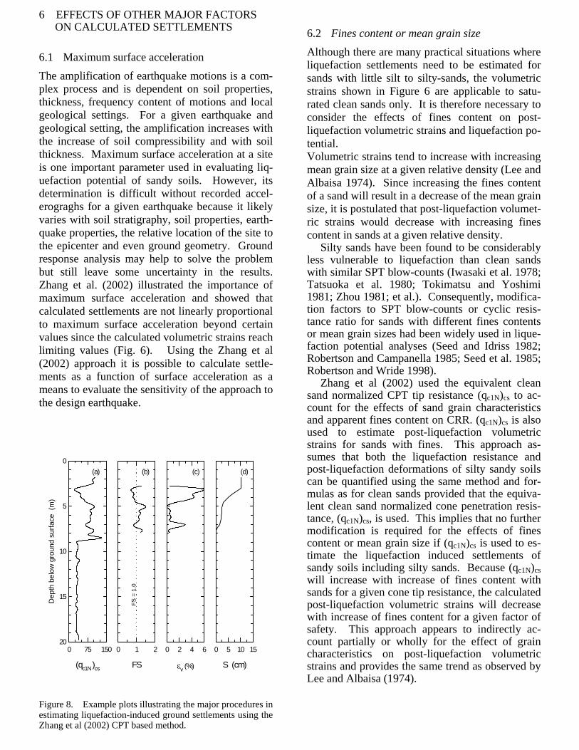
The four key plots for estimating liquefaction induced ground settlements by the CPT-based method are presented in Figure 8. Figures 8a to 8d show the profiles of equivalent clean sand normal-ized tip resistance (qc1N)cs, factor of safety FS, post-liquefaction volumetric strain εv, and lique-faction induced ground settlement S, respectively. Data in Figures 8a and 8b are from the liquefaction potential analysis. Data in Figure 8c are calculated from the results presented by Ishihara and Yo-shimine, (1992) and shown in Figure 6. The set-tlement shown in Figure 8d is obtained using Equation [10] and the volumetric strains from Fig-ure 8c.

The method by Zhang et al (2002) was evalu-ated using liquefaction-induced ground settlements from the Marina District and Treasure Island case histories damaged by liquefaction during the 1989 Loma Prieta earthquake. Good agreement between the calculated and measured liquefaction-induced ground settlements was found. Although further evaluations of the method are required with future case history data from different earthquakes and ground conditions, as they become available, it is suggested that the CPT-based method may be used to estimate liquefaction-induced settlements for low to medium risk projects and also provide pre-liminary estimates for higher risk projects.

6 EFFECTS OF OTHER MAJOR FACTORS ON CALCULATED SETTLEMENTS

6.1 Maximum surface acceleration The amplification of earthquake motions is a com-plex process and is dependent on soil properties, thickness, frequency content of motions and local geological settings. For a given earthquake and geological setting, the amplification increases with the increase of soil compressibility and with soil thickness. Maximum surface acceleration at a site is one important parameter used in evaluating liq-uefaction potential of sandy soils. However, its determination is difficult without recorded accel-erograghs for a given earthquake because it likely varies with soil stratigraphy, soil properties, earth-quake properties, the relative location of the site to the epicenter and even ground geometry. Ground response analysis may help to solve the problem but still leave some uncertainty in the results. Zhang et al. (2002) illustrated the importance of maximum surface acceleration and showed that calculated settlements are not linearly proportional to maximum surface acceleration beyond certain values since the calculated volumetric strains reach limiting values (Fig. 6). Using the Zhang et al (2002) approach it is possible to calculate settle-ments as a function of surface acceleration as a means to evaluate the sensitivity of the approach to the design earthquake.

Figure 8. Example plots illustrating the major procedures in estimating liquefaction-induced ground settlements using the Zhang et al (2002) CPT based method.

6.2 Fines content or mean grain size Although there are many practical situations where liquefaction settlements need to be estimated for sands with little silt to silty-sands, the volumetric strains shown in Figure 6 are applicable to satu-rated clean sands only. It is therefore necessary to consider the effects of fines content on post-liquefaction volumetric strains and liquefaction po-tential. Volumetric strains tend to increase with increasing mean grain size at a given relative density (Lee and Albaisa 1974). Since increasing the fines content of a sand will result in a decrease of the mean grain size, it is postulated that post-liquefaction volumet-ric strains would decrease with increasing fines content in sands at a given relative density.

Silty sands have been found to be considerably less vulnerable to liquefaction than clean sands with similar SPT blow-counts (Iwasaki et al. 1978; Tatsuoka et al. 1980; Tokimatsu and Yoshimi 1981; Zhou 1981; et al.). Consequently, modifica-tion factors to SPT blow-counts or cyclic resis-tance ratio for sands with different fines contents or mean grain sizes had been widely used in lique-faction potential analyses (Seed and Idriss 1982; Robertson and Campanella 1985; Seed et al. 1985; Robertson and Wride 1998).

Zhang et al (2002) used the equivalent clean sand normalized CPT tip resistance (qc1N)cs to ac-count for the effects of sand grain characteristics and apparent fines content on CRR. (qc1N)cs is also used to estimate post-liquefaction volumetric strains for sands with fines. This approach as-sumes that both the liquefaction resistance and post-liquefaction deformations of silty sandy soils can be quantified using the same method and for-mulas as for clean sands provided that the equiva-lent clean sand normalized cone penetration resis-tance, (qc1N)cs, is used. This implies that no further modification is required for the effects of fines content or mean grain size if (qc1N)cs is used to es-timate the liquefaction induced settlements of sandy soils including silty sands. Because (qc1N)cs will increase with increase of fines content with sands for a given cone tip resistance, the calculated post-liquefaction volumetric strains will decrease with increase of fines content for a given factor of safety. This approach appears to indirectly ac-count partially or wholly for the effect of grain characteristics on post-liquefaction volumetric strains and provides the same trend as observed by Lee and Albaisa (1974).

(qc1N )cs

0 75 150

Dep

th b

elow

gro

und

surfa

ce (

m)

0

5

10

15

20

FS

0 1 2

εv (%)

0 2 4 6

S (cm)

0 5 10 15

(a) (b) (c) (d)

FS =

1.0

6.3 Transitional zone or thin sandy soil layers It is recognized that transitional zones between soft clay layers and stiff sandy soil layers influence the calculated liquefaction-induced settlements. How-ever, the influence of the transitional zones on cal-culated (qc1N)cs, and FS has been partially counter-acted implicitly in the Robertson and Wride method. Generally, the measured tip resistance in a sandy soil layer close to a soft soil layer (usually a clayey soil layer) is smaller than the “actual” tip resistance (if no layer interface existed) and the re-sultant friction ratio is greater than the “actual” friction ratio due to the influence of the soft soil layer. As a result, the calculated value of Ic will increase, and therefore the correction factor Kc, (qc1N)cs, and FS will increase as well. (qc1N)cs and FS may be close to the “true” values in the same sandy soil layer that is not influenced by the adja-cent soft soil layer. Therefore, the calculated ground settlements would be close the “actual” values because of this implicit correction incorpo-rated within the Robertson and Wride method.

Zhang et al. (2001) took no correction in an at-tempt to quantify the influences of both the transi-tional zones and thin sandy layers on the tip resis-tance, yet achieved good agreement with the limited case history results. Making no correction for transitional zones and thin layers is conserva-tive when estimating liquefaction potential and liquefaction related deformations. Further investi-gation is required to quantify the influence of tran-sitional zones or thin sandy soil layers on calcu-lated FS and liquefaction-induced ground settlements. 6.4 Three dimensional distribution of liquefied

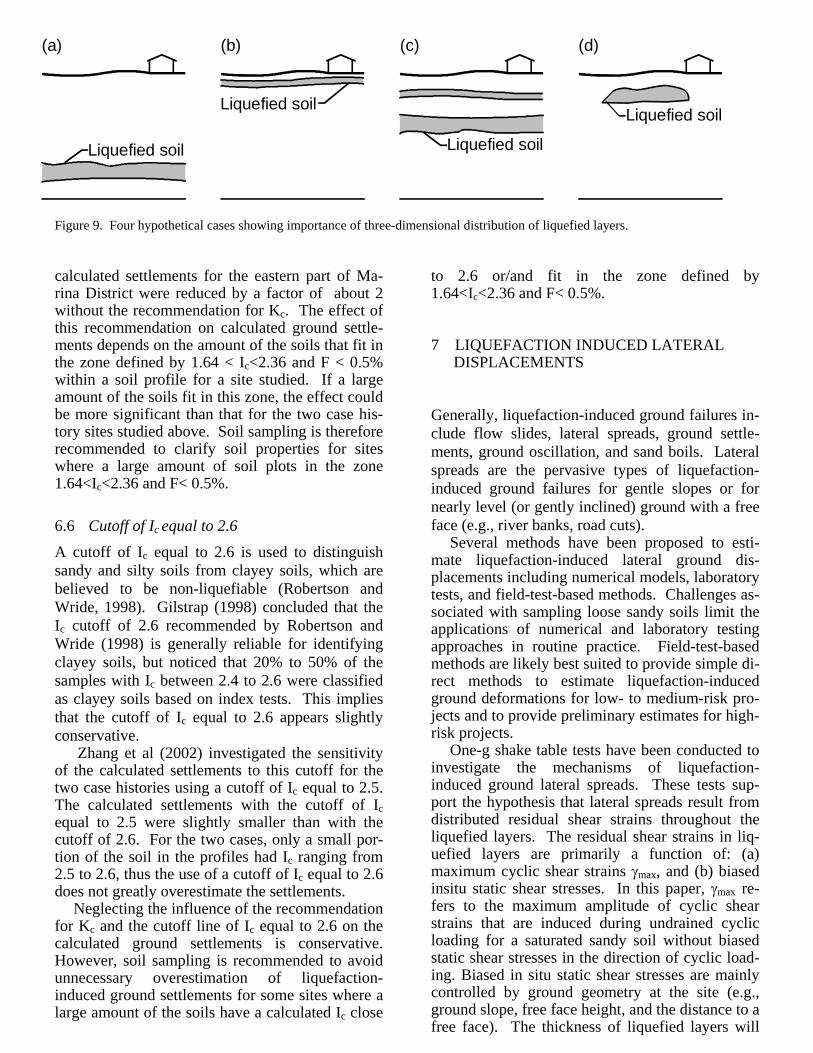
soil layers The thickness, depth and lateral distribution of liq-uefied layers will play an important role on ground surface settlements. Liquefaction of a relatively thick but deep sandy soil (see Figure 9a) may have minimal effect on the performance of an overlying structure founded on shallow foundations. How-ever, liquefaction of a near surface thin layer of soil (Figure 9b) may have major implications on the performance of the same structure.

Ishihara (1993) provided some guidance on the effect of thickness and depth to the liquefied layer on potential settlements that may be reasonable provided that the site is not susceptible to ground oscillation or lateral spread. Gilstrap (1998) con-cluded that Ishihara’s relationship for predicting surface effects may be oversimplified. As well, the application of Ishirara’s criteria in practice for cases with multiple liquefied layers (Figure 9c) is not clear.

The lateral extent of liquefied layers may also have an effect on ground surface settlements. A small locally liquefied soil zone with limited lat-eral extent (Figure 9d) would have limited extent of surface manifestation than that for a horizontally extensive liquefied soil zone with the same soil properties and vertical distribution of the liquefied layer. On the other hand, the locally liquefied soil zone may be more damaging to the engineered structures and facilities due to the potential large differential settlements. However, no quantitative study has been reported for the effect of lateral ex-tent of liquefied layers on ground surface settle-ments.

Neglecting the effect of three-dimensional dis-tribution of liquefied layers on ground surface set-tlements may result in over-estimating liquefac-tion-induced ground settlements for some sites. Engineering judgement is needed to avoid an overly conservative design. Case histories from previous earthquakes have indicated that little or no surface manifestation was observed for cases where the depth from ground surface to the top of the liquefied layer was greater than 20 m. Care is required to detect local zones of soil that may liq-uefy and to estimate the potential differential set-tlements that may occur. 6.5 Factor Kc Robertson and Wride (1998) recommended the factor Kc be set equal to 1.0 rather than using Kc of 1.0 to 2.14 when the CPT data plot in the zone de-fined by 1.64 < Ic < 2.36 and F < 0.5% to avoid confusion of very loose clean sands with denser sands containing fines. However, if the CPT data of a dense sand with fines plots in the zone (1.64 < Ic < 2.36 and F < 0.5%), the calculated (qc1N)cs value for the dense sand could be reduced by one-half. Although this recommendation is conserva-tive for evaluating liquefaction potential of sandy soils, it may result in over-estimating liquefaction-induced ground settlements for sites with denser sands containing fines that fit in that zone. This seems to be true for some of the CPT soundings in the two case histories studied by Zhang et al (2002). For example, based on soil profiles, CPT profiles, and engineering judgment, a portion of the soil that should have been assessed as dense sand containing fines, was classified as very loose clean sand with Kc equal to 1.0.

Zhang et al (2002) showed that when the set-tlements for the two case histories were recalcu-lated without following the recommendation of Kc equal to 1.0 for 1.64 < Ic < 2.36 and F < 0.5%, there was almost no effect for the western and cen-tral parts of Marina District and only small (up to 14%) effects for Treasure Island. However the

Liquefied soil

Liquefied soil

Liquefied soil

Liquefied soil

(a) (b) (c) (d)

Figure 9. Four hypothetical cases showing importance of three-dimensional distribution of liquefied layers.

calculated settlements for the eastern part of Ma-rina District were reduced by a factor of about 2 without the recommendation for Kc. The effect of this recommendation on calculated ground settle-ments depends on the amount of the soils that fit in the zone defined by 1.64 < Ic<2.36 and F < 0.5% within a soil profile for a site studied. If a large amount of the soils fit in this zone, the effect could be more significant than that for the two case his-tory sites studied above. Soil sampling is therefore recommended to clarify soil properties for sites where a large amount of soil plots in the zone 1.64<Ic<2.36 and F< 0.5%. 6.6 Cutoff of Ic equal to 2.6 A cutoff of Ic equal to 2.6 is used to distinguish sandy and silty soils from clayey soils, which are believed to be non-liquefiable (Robertson and Wride, 1998). Gilstrap (1998) concluded that the Ic cutoff of 2.6 recommended by Robertson and Wride (1998) is generally reliable for identifying clayey soils, but noticed that 20% to 50% of the samples with Ic between 2.4 to 2.6 were classified as clayey soils based on index tests. This implies that the cutoff of Ic equal to 2.6 appears slightly conservative.

Zhang et al (2002) investigated the sensitivity of the calculated settlements to this cutoff for the two case histories using a cutoff of Ic equal to 2.5. The calculated settlements with the cutoff of Ic equal to 2.5 were slightly smaller than with the cutoff of 2.6. For the two cases, only a small por-tion of the soil in the profiles had Ic ranging from 2.5 to 2.6, thus the use of a cutoff of Ic equal to 2.6 does not greatly overestimate the settlements.

Neglecting the influence of the recommendation for Kc and the cutoff line of Ic equal to 2.6 on the calculated ground settlements is conservative. However, soil sampling is recommended to avoid unnecessary overestimation of liquefaction-induced ground settlements for some sites where a large amount of the soils have a calculated Ic close

to 2.6 or/and fit in the zone defined by 1.64<Ic<2.36 and F< 0.5%.

7 LIQUEFACTION INDUCED LATERAL DISPLACEMENTS

Generally, liquefaction-induced ground failures in-clude flow slides, lateral spreads, ground settle-ments, ground oscillation, and sand boils. Lateral spreads are the pervasive types of liquefaction-induced ground failures for gentle slopes or for nearly level (or gently inclined) ground with a free face (e.g., river banks, road cuts).

Several methods have been proposed to esti-mate liquefaction-induced lateral ground dis-placements including numerical models, laboratory tests, and field-test-based methods. Challenges as-sociated with sampling loose sandy soils limit the applications of numerical and laboratory testing approaches in routine practice. Field-test-based methods are likely best suited to provide simple di-rect methods to estimate liquefaction-induced ground deformations for low- to medium-risk pro-jects and to provide preliminary estimates for high-risk projects.

One-g shake table tests have been conducted to investigate the mechanisms of liquefaction-induced ground lateral spreads. These tests sup-port the hypothesis that lateral spreads result from distributed residual shear strains throughout the liquefied layers. The residual shear strains in liq-uefied layers are primarily a function of: (a) maximum cyclic shear strains γmax, and (b) biased insitu static shear stresses. In this paper, γmax re-fers to the maximum amplitude of cyclic shear strains that are induced during undrained cyclic loading for a saturated sandy soil without biased static shear stresses in the direction of cyclic load-ing. Biased in situ static shear stresses are mainly controlled by ground geometry at the site (e.g., ground slope, free face height, and the distance to a free face). The thickness of liquefied layers will

Factor of safety, FS

0.0 0.5 1.0 1.5 2.0

Max

imum

cyc

lic s

hear

stra

in,

γ max

(%

)

0

10

20

30

40

50

60

90%

50%

60%

80%

70%

Dr = 40%

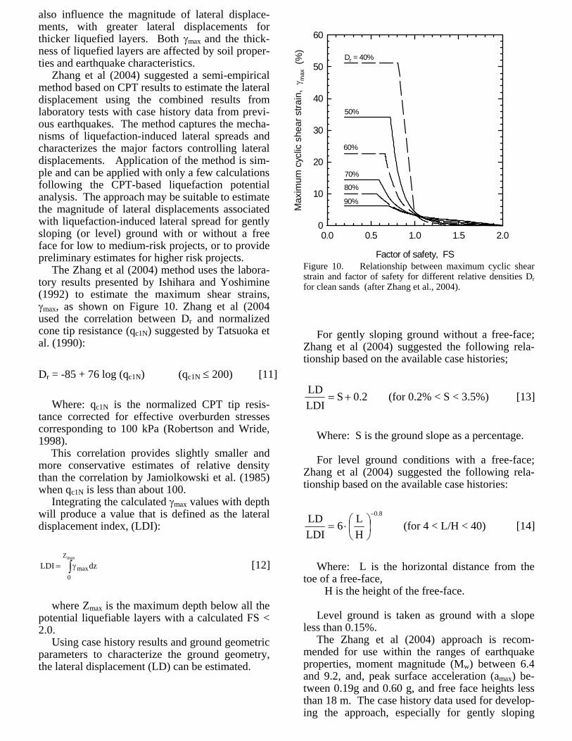
also influence the magnitude of lateral displace-ments, with greater lateral displacements for thicker liquefied layers. Both γmax and the thick-ness of liquefied layers are affected by soil proper-ties and earthquake characteristics.

Zhang et al (2004) suggested a semi-empirical method based on CPT results to estimate the lateral displacement using the combined results from laboratory tests with case history data from previ-ous earthquakes. The method captures the mecha-nisms of liquefaction-induced lateral spreads and characterizes the major factors controlling lateral displacements. Application of the method is sim-ple and can be applied with only a few calculations following the CPT-based liquefaction potential analysis. The approach may be suitable to estimate the magnitude of lateral displacements associated with liquefaction-induced lateral spread for gently sloping (or level) ground with or without a free face for low to medium-risk projects, or to provide preliminary estimates for higher risk projects.

The Zhang et al (2004) method uses the labora-tory results presented by Ishihara and Yoshimine (1992) to estimate the maximum shear strains, γmax, as shown on Figure 10. Zhang et al (2004 used the correlation between Dr and normalized cone tip resistance (qc1N) suggested by Tatsuoka et al. (1990):

Dr = -85 + 76 log (qc1N) (qc1N ≤ 200) [11] Where: qc1N is the normalized CPT tip resis-

tance corrected for effective overburden stresses corresponding to 100 kPa (Robertson and Wride, 1998).

This correlation provides slightly smaller and more conservative estimates of relative density than the correlation by Jamiolkowski et al. (1985) when qc1N is less than about 100.

Integrating the calculated γmax values with depth will produce a value that is defined as the lateral displacement index, (LDI):

dzLDImaxZ

0max∫ γ= [12]

where Zmax is the maximum depth below all the

potential liquefiable layers with a calculated FS < 2.0.

Using case history results and ground geometric parameters to characterize the ground geometry, the lateral displacement (LD) can be estimated.

Figure 10. Relationship between maximum cyclic shear strain and factor of safety for different relative densities Dr for clean sands (after Zhang et al., 2004).

For gently sloping ground without a free-face;

Zhang et al (2004) suggested the following rela-tionship based on the available case histories;

2.0SLDILD

+= (for 0.2% < S < 3.5%) [13]

Where: S is the ground slope as a percentage. For level ground conditions with a free-face;

Zhang et al (2004) suggested the following rela-tionship based on the available case histories:

8.0

HL6

LDILD −

⎟⎠⎞

⎜⎝⎛⋅= (for 4 < L/H < 40) [14]

Where: L is the horizontal distance from the

toe of a free-face, H is the height of the free-face. Level ground is taken as ground with a slope

less than 0.15%. The Zhang et al (2004) approach is recom-

mended for use within the ranges of earthquake properties, moment magnitude (Mw) between 6.4 and 9.2, and, peak surface acceleration (amax) be-tween 0.19g and 0.60 g, and free face heights less than 18 m. The case history data used for develop-ing the approach, especially for gently sloping

ground without a free face, were dominantly from two Japanese case histories associated with the 1964 Niigata and 1983 Nihonkai-Chubu earth-quakes, where the liquefied soils were mainly clean sand only. The values for the geometric pa-rameters used in developing the approach were within limited ranges, as specified in Equations [13] and [14]. It is recommended that the ap-proach not be used when the values of the geomet-ric parameters go beyond the specified ranges.

The approach by Zhang et al (2004) is suitable to estimate the magnitude of lateral displacements associated with liquefaction-induced lateral spread for gently sloping (or level) ground with or without a free face for low to medium-risk projects, or to provide preliminary estimates for higher risk pro-jects. Given the complexity of liquefaction-induced lateral spreads, considerable variations in magnitude and distribution of lateral displacements are expected. Generally, the calculated lateral dis-placements using the proposed approach for the available case histories showed variations between 50% and 200% of measured values. The accuracy of “measured” lateral displacements for most case histories is about ± 0.1 to ± 1.92 m. Therefore, it is unrealistic to expect the accuracy of estimated lateral displacements be within ± 0.1 m. The reli-ability of the proposed approach can be fully evaluated only over time with more available case histories.

The approach by Zhang et al (2004) was devel-oped using case history data with limited ranges of earthquake parameters, soil properties, and geo-metric parameters. Therefore, it is not recom-mended that the approach be applied for values of input parameters beyond the specified ranges. En-gineering judgement and caution should be always exercised in applying the proposed approach and in interpreting the results. Additional new data are required to further evaluate and update the pro-posed approach.

8 FLOW LIQUEFACTION

When a soil is strain softening there is the potential for instability. The key response parameter re-quired to estimate if a flow slide would occur is the minimum (residual or liquefied) undrained shear strength, smin following strain softening. Methods have been suggested to estimate the minimum (liq-uefied) undrained shear strength of clean sands from penetration resistance based on case histories (Seed and Harder, 1990; Stark and Mesri, 1992). A recent re-evaluation of these case histories (Wride et al., 1998) has questioned the validity of the proposed correlation. Recent research has also

shown the importance of direction of loading on the minimum undrained shear strength of sands. The minimum undrained shear strength in triaxial compression (TC) loading is higher than that in simple shear (SS), which in turn, is larger than that in triaxial extension (TE). The difference is less as the sand becomes looser. Hence, the appropriate undrained shear strength to be used in a stability analyses will be a function of direction of loading. This has been recognized for some time in clay soils (Bjerrum, 1972).

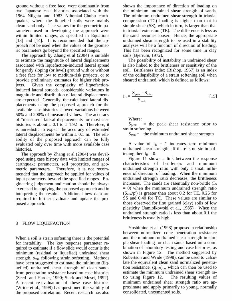
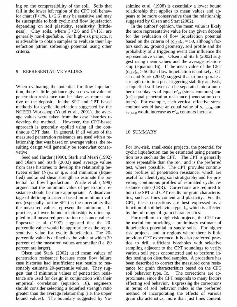
The possibility of instability in undrained shear is also linked to the brittleness or sensitivity of the soil. Brittleness index (Bishop, 1967) is an index of the collapsibility of a strain softening soil when sheared undrained, which is defined as follows:

IB = peak

minpeak

SS - S

[15]

Where: Speak = the peak shear resistance prior to

strain softening Smin = the minimum undrained shear strength A value of IB = 1 indicates zero minimum

undrained shear strength. If there is no strain sof-tening then IB = 0.

Figure 11 shows a link between the response characteristics of brittleness and minimum undrained strength ratio with only a small influ-ence of direction of loading. When the minimum undrained strength ratio decreases, the brittleness increases. The sands are essentially non-brittle (IB = 0) when the minimum undrained strength ratio (Smin/p') is greater than about 0.2 for TE, 0.25 for SS and 0.40 for TC. These values are similar to those observed for fine grained (clay) soils of low plasticity (Jamiolkowski et al., 1985). When the undrained strength ratio is less than about 0.1 the brittleness is usually high.

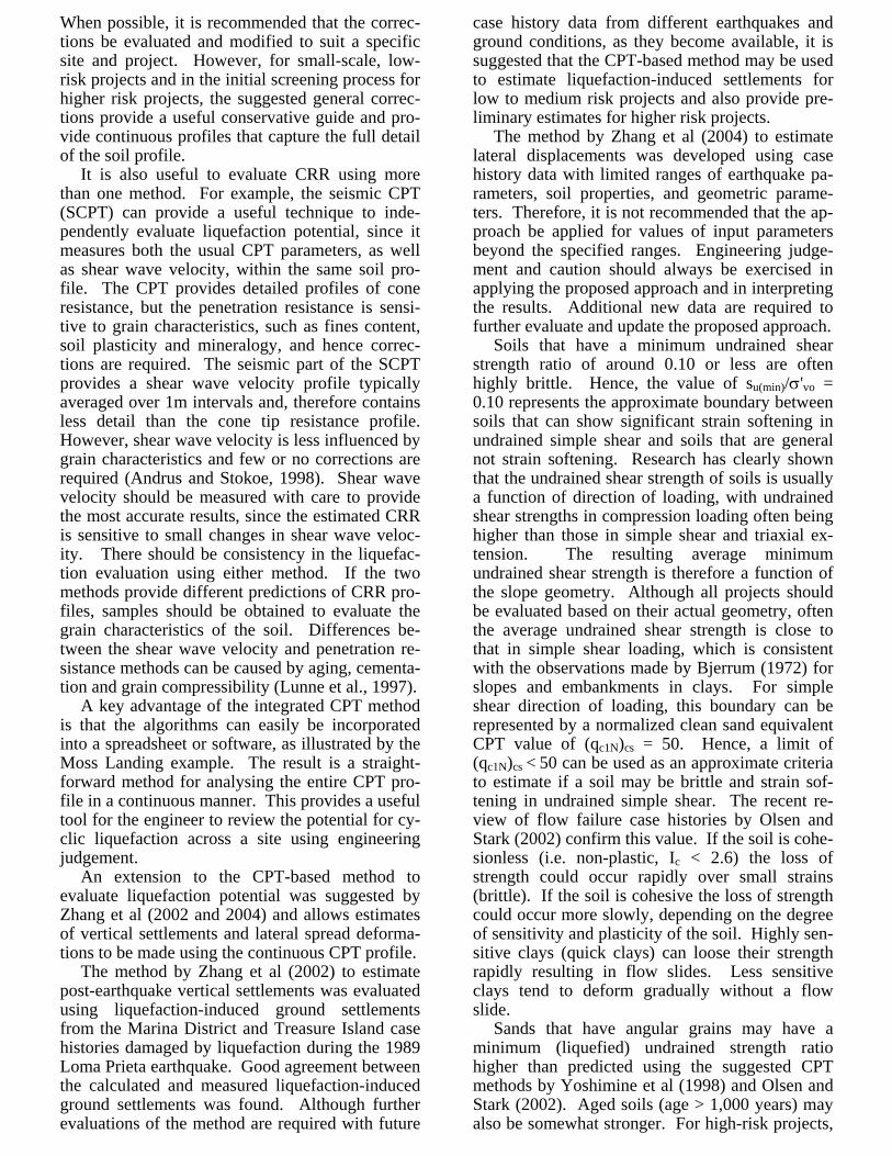
Yoshimine et al. (1998) proposed a relationship

between normalized cone penetration resistance and the minimum undrained shear strength in sim-ple shear loading for clean sands based on a com-bination of laboratory testing and case histories, as shown in Figure 12. The method suggested by Robertson and Wride (1998), can be used to calcu-late the equivalent clean sand normalized penetra-tion resistance, (qc1N)cs, which can then be used to estimate the minimum undrained shear strength ra-tio using Figure 12. The resulting values of minimum undrained shear strength ratio are ap-proximate and apply primarily to young, normally consolidated, uncemented soils.

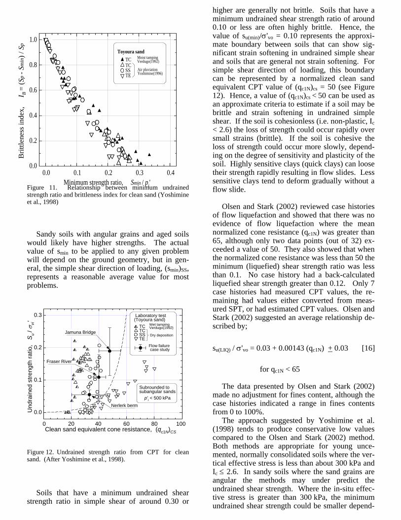
Figure 11. Relationship between minimum undrained strength ratio and brittleness index for clean sand (Yoshimine et al., 1998)

Sandy soils with angular grains and aged soils

would likely have higher strengths. The actual value of smin to be applied to any given problem will depend on the ground geometry, but in gen-eral, the simple shear direction of loading, (smin)SS, represents a reasonable average value for most problems.

Figure 12. Undrained strength ratio from CPT for clean sand. (After Yoshimine et al., 1998).

Soils that have a minimum undrained shear

strength ratio in simple shear of around 0.30 or

higher are generally not brittle. Soils that have a minimum undrained shear strength ratio of around 0.10 or less are often highly brittle. Hence, the value of su(min)/σ'vo = 0.10 represents the approxi-mate boundary between soils that can show sig-nificant strain softening in undrained simple shear and soils that are general not strain softening. For simple shear direction of loading, this boundary can be represented by a normalized clean sand equivalent CPT value of (qc1N)cs = 50 (see Figure 12). Hence, a value of (qc1N)cs < 50 can be used as an approximate criteria to estimate if a soil may be brittle and strain softening in undrained simple shear. If the soil is cohesionless (i.e. non-plastic, Ic < 2.6) the loss of strength could occur rapidly over small strains (brittle). If the soil is cohesive the loss of strength could occur more slowly, depend-ing on the degree of sensitivity and plasticity of the soil. Highly sensitive clays (quick clays) can loose their strength rapidly resulting in flow slides. Less sensitive clays tend to deform gradually without a flow slide.

0.0 0.1 0.2 0.3 0.40.0

0.2

0.4

0.6

0.8

1.0Toyoura sand TC TC SS TE

Moist tampingVerdugo(1992)

Air pluviationYoshimine(1996)

Brit

tlene

ss in

dex,

I

B =

(Sp

- Sm

in) /

Sp

Minimum strength ratio, Smin / pi'

Olsen and Stark (2002) reviewed case histories

of flow liquefaction and showed that there was no evidence of flow liquefaction where the mean normalized cone resistance (qc1N) was greater than 65, although only two data points (out of 32) ex-ceeded a value of 50. They also showed that when the normalized cone resistance was less than 50 the minimum (liquefied) shear strength ratio was less than 0.1. No case history had a back-calculated liquefied shear strength greater than 0.12. Only 7 case histories had measured CPT values, the re-maining had values either converted from meas-ured SPT, or had estimated CPT values. Olsen and Stark (2002) suggested an average relationship de-scribed by;

0 20 40 60 80 100

0.0

0.1

0.2

0.3

Clean sand equivalent cone resistance, (qc1N)CS

Laboratory test(Toyoura sand) TC TC SS TE Flow failure case study

Wet tampingVerdugo(1992)

Dry deposition

Nerlerk berm

Jamuna Bridge

Fraser River

Und

rain

ed s

treng

th ra

tio,

Su / σ

vi'

Subrounded tosubangular sands

p'i < 500 kPa

su(LIQ) / σ'vo = 0.03 + 0.00143 (qc1N) + 0.03 [16]

for qc1N < 65 The data presented by Olsen and Stark (2002)

made no adjustment for fines content, although the case histories indicated a range in fines contents from 0 to 100%.

The approach suggested by Yoshimine et al. (1998) tends to produce conservative low values compared to the Olsen and Stark (2002) method. Both methods are appropriate for young unce-mented, normally consolidated soils where the ver-tical effective stress is less than about 300 kPa and Ic ≤ 2.6. In sandy soils where the sand grains are angular the methods may under predict the undrained shear strength. Where the in-situ effec-tive stress is greater than 300 kPa, the minimum undrained shear strength could be smaller depend-

ing on the compressibility of the soil. Soils that fall in the lower left region of the CPT soil behav-ior chart (F<1%, Ic>2.6) may be sensitive and may be susceptible to both cyclic and flow liquefaction depending on soil plasticity, sensitivity (brittle-ness). Clay soils, where Ic>2.6 and F>1%, are generally non-liquefiable. For high-risk projects, it is advisable to obtain samples to evaluate their liq-uefaction (strain softening) potential using other criteria.

9 REPRESENTATIVE VALUES

When evaluating the potential for flow liquefac-tion, there is little guidance given on what value of penetration resistance can be taken as representa-tive of the deposit. In the SPT and CPT based methods for cyclic liquefaction suggested by the NCEER Workshop (Youd et al., 2001), the aver-age values were taken from the case histories to develop the method. However, the CPT-based approach is generally applied using all the con-tinuous CPT data. In general, if all values of the measured penetration resistance are used with a re-lationship that was based on average values, the re-sulting design will generally be somewhat conser-vative.

Seed and Harder (1990), Stark and Mesri (1992) and Olson and Stark (2002) used average values from case histories to develop the relationship be-tween either (N1)60 or qc1N and minimum (lique-fied) undrained shear strength to estimate the po-tential for flow liquefaction. Wride et al. (1998) argued that the minimum value of penetration re-sistance should be more appropriate. A disadvan-tage of defining a criteria based on minimum val-ues (especially for the SPT) is the uncertainty that the measured values represent the minimum. In practice, a lower bound relationship is often ap-plied to all measured penetration resistance values. Popescue et al. (1997) suggested that the 20-percentile value would be appropriate as the repre-sentative value for cyclic liquefaction. The 20-percentile value is defined as the value at which 20 percent of the measured values are smaller (i.e. 80 percent are larger).

Olsen and Stark (2002) used mean values of penetration resistance because most flow failure case histories had insufficient test results to rea-sonably estimate 20-percentile values. They sug-gest that if minimum values of penetration resis-tance are used for design in conjunction with their empirical correlation (equation 16), engineers should consider selecting a liquefied strength ratio greater than the average relationship (i.e. the upper bound values). The boundary suggested by Yo-

shimine et al. (1998) is essentially a lower bound relationship that applies to mean values and ap-pears to be more conservative than the relationship suggested by Olsen and Start (2002).

In the authors' opinion, the mean value is likely the more representative value for any given deposit for the evaluation of flow liquefaction potential based on the criteria of (qc1N)cs = 50, although fac-tors such as, ground geometry, soil profile and the probability of a triggering event can influence the representative value. Olsen and Stark (2002) sug-gest using mean values and the average relation-ship (equation 16). If the mean value of the CPT (qc1N)cs > 50 than flow liquefaction is unlikely. Ol-sen and Stark (2002) suggest that to incorporate a strength ratio in a post-triggering stability analysis, a liquefied soil layer can be separated into a num-ber of sublayers of equal σ'vo (stress contours) and (or) equal penetration resistance (penetration con-tours). For example, each vertical effective stress contour would have an equal value of su (LIQ), and su (LIQ) would increase as σ'vo contours increase.

10 SUMMARY

For low-risk, small-scale projects, the potential for cyclic liquefaction can be estimated using penetra-tion tests such as the CPT. The CPT is generally more repeatable than the SPT and is the preferred test, where possible. The CPT provides continu-ous profiles of penetration resistance, which are useful for identifying soil stratigraphy and for pro-viding continuous profiles of estimated cyclic re-sistance ratio (CRR). Corrections are required to both the SPT and CPT results for grain characteris-tics, such as fines content and plasticity. For the CPT, these corrections are best expressed as a function of soil behavior type, Ic, which is affected by the full range of grain characteristics.

For medium- to high-risk projects, the CPT can be useful for providing a preliminary estimate of liquefaction potential in sandy soils. For higher risk projects, and in regions where there is little previous CPT experience, it is also preferred prac-tice to drill sufficient boreholes with selective sampling adjacent to the CPT soundings to verify various soil types encountered and to perform in-dex testing on disturbed samples. A procedure has been described to correct the measured cone resis-tance for grain characteristics based on the CPT soil behavior type, Ic. The corrections are ap-proximate, since the CPT responds to many factors affecting soil behavior. Expressing the corrections in terms of soil behavior index is the preferred method of incorporating the effects of various grain characteristics, more than just fines content.

When possible, it is recommended that the correc-tions be evaluated and modified to suit a specific site and project. However, for small-scale, low-risk projects and in the initial screening process for higher risk projects, the suggested general correc-tions provide a useful conservative guide and pro-vide continuous profiles that capture the full detail of the soil profile.

It is also useful to evaluate CRR using more than one method. For example, the seismic CPT (SCPT) can provide a useful technique to inde-pendently evaluate liquefaction potential, since it measures both the usual CPT parameters, as well as shear wave velocity, within the same soil pro-file. The CPT provides detailed profiles of cone resistance, but the penetration resistance is sensi-tive to grain characteristics, such as fines content, soil plasticity and mineralogy, and hence correc-tions are required. The seismic part of the SCPT provides a shear wave velocity profile typically averaged over 1m intervals and, therefore contains less detail than the cone tip resistance profile. However, shear wave velocity is less influenced by grain characteristics and few or no corrections are required (Andrus and Stokoe, 1998). Shear wave velocity should be measured with care to provide the most accurate results, since the estimated CRR is sensitive to small changes in shear wave veloc-ity. There should be consistency in the liquefac-tion evaluation using either method. If the two methods provide different predictions of CRR pro-files, samples should be obtained to evaluate the grain characteristics of the soil. Differences be-tween the shear wave velocity and penetration re-sistance methods can be caused by aging, cementa-tion and grain compressibility (Lunne et al., 1997).

A key advantage of the integrated CPT method is that the algorithms can easily be incorporated into a spreadsheet or software, as illustrated by the Moss Landing example. The result is a straight-forward method for analysing the entire CPT pro-file in a continuous manner. This provides a useful tool for the engineer to review the potential for cy-clic liquefaction across a site using engineering judgement.

An extension to the CPT-based method to evaluate liquefaction potential was suggested by Zhang et al (2002 and 2004) and allows estimates of vertical settlements and lateral spread deforma-tions to be made using the continuous CPT profile.

The method by Zhang et al (2002) to estimate post-earthquake vertical settlements was evaluated using liquefaction-induced ground settlements from the Marina District and Treasure Island case histories damaged by liquefaction during the 1989 Loma Prieta earthquake. Good agreement between the calculated and measured liquefaction-induced ground settlements was found. Although further evaluations of the method are required with future

case history data from different earthquakes and ground conditions, as they become available, it is suggested that the CPT-based method may be used to estimate liquefaction-induced settlements for low to medium risk projects and also provide pre-liminary estimates for higher risk projects.

The method by Zhang et al (2004) to estimate lateral displacements was developed using case history data with limited ranges of earthquake pa-rameters, soil properties, and geometric parame-ters. Therefore, it is not recommended that the ap-proach be applied for values of input parameters beyond the specified ranges. Engineering judge-ment and caution should always be exercised in applying the proposed approach and in interpreting the results. Additional new data are required to further evaluate and update the proposed approach.

Soils that have a minimum undrained shear strength ratio of around 0.10 or less are often highly brittle. Hence, the value of su(min)/σ'vo = 0.10 represents the approximate boundary between soils that can show significant strain softening in undrained simple shear and soils that are general not strain softening. Research has clearly shown that the undrained shear strength of soils is usually a function of direction of loading, with undrained shear strengths in compression loading often being higher than those in simple shear and triaxial ex-tension. The resulting average minimum undrained shear strength is therefore a function of the slope geometry. Although all projects should be evaluated based on their actual geometry, often the average undrained shear strength is close to that in simple shear loading, which is consistent with the observations made by Bjerrum (1972) for slopes and embankments in clays. For simple shear direction of loading, this boundary can be represented by a normalized clean sand equivalent CPT value of (qc1N)cs = 50. Hence, a limit of (qc1N)cs < 50 can be used as an approximate criteria to estimate if a soil may be brittle and strain sof-tening in undrained simple shear. The recent re-view of flow failure case histories by Olsen and Stark (2002) confirm this value. If the soil is cohe-sionless (i.e. non-plastic, Ic < 2.6) the loss of strength could occur rapidly over small strains (brittle). If the soil is cohesive the loss of strength could occur more slowly, depending on the degree of sensitivity and plasticity of the soil. Highly sen-sitive clays (quick clays) can loose their strength rapidly resulting in flow slides. Less sensitive clays tend to deform gradually without a flow slide.

Sands that have angular grains may have a minimum (liquefied) undrained strength ratio higher than predicted using the suggested CPT methods by Yoshimine et al (1998) and Olsen and Stark (2002). Aged soils (age > 1,000 years) may also be somewhat stronger. For high-risk projects,

the proposed CPT criteria (based on (qc1N)cs < 50) provides a useful screening technique to identify potentially critical zones where flow liquefaction may be possible. For low risk projects, the pro-posed CPT methods will generally provide a con-servative estimate of the minimum undrained shear strength ratio in simple shear loading. The pro-posed relationship conservatively estimates the minimum (liquefied) undrained shear strength ratio for a soil structure that contains extensive amounts of loose sandy soils with impeded drainage, such as thick deposits of loose interbedded sands and silts. In soil structures where drainage and con-solidation of the liquefied layer can occur during and immediately after the earthquake, higher val-ues of undrained shear strength will likely exist. Such conditions may exist in a thin deposit with free drainage to the ground surface or a deposit in-terbedded with extensive pervious gravel layers.

ACKNOWLEDGEMENTS

This paper is a summary of many years of re-

search that have involved many colleagues and graduate students as well as support by the Natural Science and Engineering Research Council of Can-ada (NSERC).

REFERENCES

Andrus, R.D., and Stokoe, K.H. 1998. Guidelines for evaluation of liquefaction resistance using shear wave velocity. Proceedings of the NCEER (National Center for Earthquake Engi-neering Research) workshop on evaluation of liquefaction resistance of soils, Salt Lake City, Utah, January 1996, T.L. Youd and I.M. Idriss (eds.), NCEER-97-0022, 89-128.

Bishop, A.W. 1967. Progressive failure – with special reference to the mechanism causing it. Panel discussion. Proceedings of the Geotech-nical Conference, Oslo, Norway, 2: 142-150.

Bjerrum, L., 1972, Embankments on soft ground. Proceedings of Specialty Conference on Per-formance of Earth and Earth-supported struc-tures, Lafayette, Indiana, 2: 1-54.

Bartlett, S.F., and Youd, T.L. 1995. Empirical prediction of liquefaction-induced lateral spread. Journal of Geotechnical Engineering, ASCE, 121(4): 316-328.

Boulanger, R.W., Mejia, L.H., and Irdiss, I.M. 1997. Liquefaction at Moss Landing during Loma Prieta earthquake. Journal of Geotech-nical and Geoenvironmental Engineering, ASCE, 123(5): 453-468.

Ishihara, K., 1993. Liquefaction and flow failure during earthquakes. 33rd Rankine Lecture, Geotechnique, 43(3): 349-415.

Ishihara, K., and Yoshimine, M. 1992. Evaluation of settlements in sand deposits following lique-faction during earthquakes. Soils and Founda-tions, 32(1): 173-188.

Iwasaki, T., Tatsuoka, F., Tokida, K., and Yasuda, S. 1978. A practical method for assessing soil liquefaction potential based on case studies at various sites in Japan. Proceeding of the Sec-ond International Conference of Microzona-tion, San Francisco, CA, Vol. 2, pp.885-896.

Jamiolkowski, M., Ladd, C.C., Germaine, J.T., and Lancellotta, R. 1985. New developments in field and laboratory testing of soils. In Pro-ceedings of the Eleventh International Confer-ence on Soil Mechanics and Foundation Engi-neering, San Francisco, 12-16 August, Vol. 1, pp. 57-153.

Juang, C. H., Chen, C. J., and Tien, Y. M. 1999a. Appraising CPT-based liquefaction resistance evaluation methods -- artificial neural network approach. Canadian Geotechnical Journal, 36(3): 443-454.

Juang, C. H., Rosowsky, D. V., and Tang, W. H. 1999b. Reliability-based method for assessing liquefaction potential of soils. Journal of Geo-technical and Geoenvironmental Engineering, ASCE, 125(8): 684-689.

Lee, K. L., and Albaisa, A. 1974. Earthquake in-duced settlements in saturated sands. Journal of Geotechnical Engineering, ASCE, 100(GT4): 387-406.

NCEER 1997. Proceeding of the NCEER Work-shop on Evaluation of Liquefaction Resistance of Soils, Edited by Youd, T. L., and Idriss, I. M., Technical Report NCEER-97-0022, Salt Lake City, Utah, Decemeber 31, 1997.

Olsen, R.S., and Malone, P.G. 1988. Soil classifi-cation and site characterization using the cone penetrometer test. Penetration Testing 1988, ISOPT-1, Edited by De Ruiter, Balkema, Rot-terdam, 2: 887-893.

Olsen, S.M. and Stark, T.D., 2002. Liquefied Strength ratio from liquefaction flow failure case histories. Canadian Geotechnical Journal, 39: 629-647

Popescu, R., Prevost, J.H., and Deodatis, G., 1997. Effects od spacial variability on soil liquefac-tion: some design recommendations. Geotech-nique, 47(5): 1019-1036

Robertson, P.K., 1990. Soil Classification using the CPT. Canadian Geotechnical Journal. 27(1),151-158.

Robertson, P.K., and Wride C.E. 1998. Evaluat-ing cyclic liquefaction potential using the CPT. Canadian Geotechnical Journal, 35(3): 442-459.

Robertson, P. K., and Campanella, R. G. 1985. Liquefaction potential of sands using the cone penetration test. Journal of Geotechnical Engi-neering, ASCE, 22(3): 298-307.

Seed, H.B. 1979. Soil liquefaction and cyclic mobility evaluation for level ground during earthquakes. Journal of Geotechnical Engineer-ing Division, ASCE, 105(GT2): 201-255.

Seed, H. B., and Idriss, I. M. 1971. Simplified procedure for evaluation soil liquefaction poten-tial. Journal of the Soil Mechanics and Founda-tions Division, ASCE, 97(SM9): 1249-1273.

Seed, H. B., and Idriss, I. M. 1982. Ground mo-tions and soil liquefaction during earthquakes. Earthquake Engineering Research Institute, p.134.

Seed, H. B., Tokimatsu, K., Harder, L. F., and Chung, R. M. 1985. Influence of SPT proce-dures in soil liquefaction resistance evaluations. Journal of Geotechnical Engineering, ASCE, 111(12): 1425-1440.

Seed, R. B., and Harder, L. F. 1990. SPT-based analysis of cyclic pore pressure generation and undrained residual strength. Proceedings H. B. Seed Memorial Symp., Vol. 2, BiTech Pub-lishers, Vancouver, BC, May, pp.351-376.

Stark, T.D., and Mesri, G.M., 1992. Undrained shear strength of liquefied sands for stability analysis. Journal of Geotechnical Engineering. ASCE, 118 (11): 1727-1747.

Tatsuoka, F., Iwasaki, T., Tokida, K., Yasuda, S., Hirose, M., Imai, T., and Kon-no, M. 1980. Standard penetration tests and soil liquefaction potential evaluation. Soils and Foundations, JSSMFE, 20(4): 95-111.

Tokimatsu, K. and Yoshimi, Y. 1981. Field corre-lation of soil liquefaction with SPT and grain size. Proceedings of Eight World Conference on Earthquake Engineering, San Francisco, CA, 95-102.

Yoshimine, M., Robertson, P.K., and Wride, C.E., 1998, Undrained shear strength of clean sands, Accepted for publication in the Canadian Geo-technical Journal.

Wride, C.E., McRoberts, E.C. and Robertson, P.K., 1998. Reconsideration of Case Histories for Estimating Undrained Shear strength in Sandy soils. Accepted for publication in the Canadian Geotechnical Journal.

Youd, T.L., Idriss, I.M, Andrus, R.D., Arango, I., Castro, G., Christian, J.T., Dobry, R., Finn, W.D.L., Harder, L.F., Hynes, M.E., Ishihara, K., Koester, J.P., Liao, S.S.C., Marcuson, W.F., Martin, G.R., Mitchell, J.K., Moriwaki, Y., Power, M.S., Robertson, P.K., Seed, R.B., Stokoe, K.H. 2001. Liquefaction resistance of soils: summary report from the 1996 NCEER and 1998 NCEER/NSF Workshops on evalua-tion of liquefaction resistance of soils. Journal of Geotechnical and Geoenvironmental Engi-neering, 127(4): 297 – 313.

Zhang, G., Robertson, P.K. and Brachman, R.W.I, 2002. Estimating liquefaction-induced ground settlements from CPT for level ground. Cana-dian Geotechnical Journal, 39: 1168-1180

Zhang, G., Robertson, P.K. and Brachman, R.W.I, 2004. Estimating liquefaction-induced lateral displacements using the SPT or CPT. Journal of Geotechnical and Geoenvironmental Engi-neering.

Zhou, S. G. 1981. Influence of fines on evaluat-ing liquefaction of sand by CPT. Proceedings of International Conference on Recent Ad-vances in Geotechnical Earthquake Engineer-ing and Soil Dynamics, St. Louis, MO, 1, 167-172.