unit 5: polynomial interpolation - matematikcentrum | … · 2015-04-12 · unit 5: polynomial...
TRANSCRIPT
Unit 5: Polynomial Interpolation
We denote (as above) by Pn the linear space (vector space) of all polynomialsof (max-) degree n.
Definition. [–] Let (xi, yi), i = 0 : n be n + 1 pairs of real numbers(typically measurement data)A polynomial p ∈ Pn interpolates these data points if
p(xk) = yk k = 0 : n
holds.
We assume in the sequel that the xi are distinct.
C. Fuhrer/ A. Sopasakis: FMN050/FMNF01-2015
81
5.1: Polynomial Interpolation
0 1 2 3 4 5 6-2
-1
0
1
2
3
4
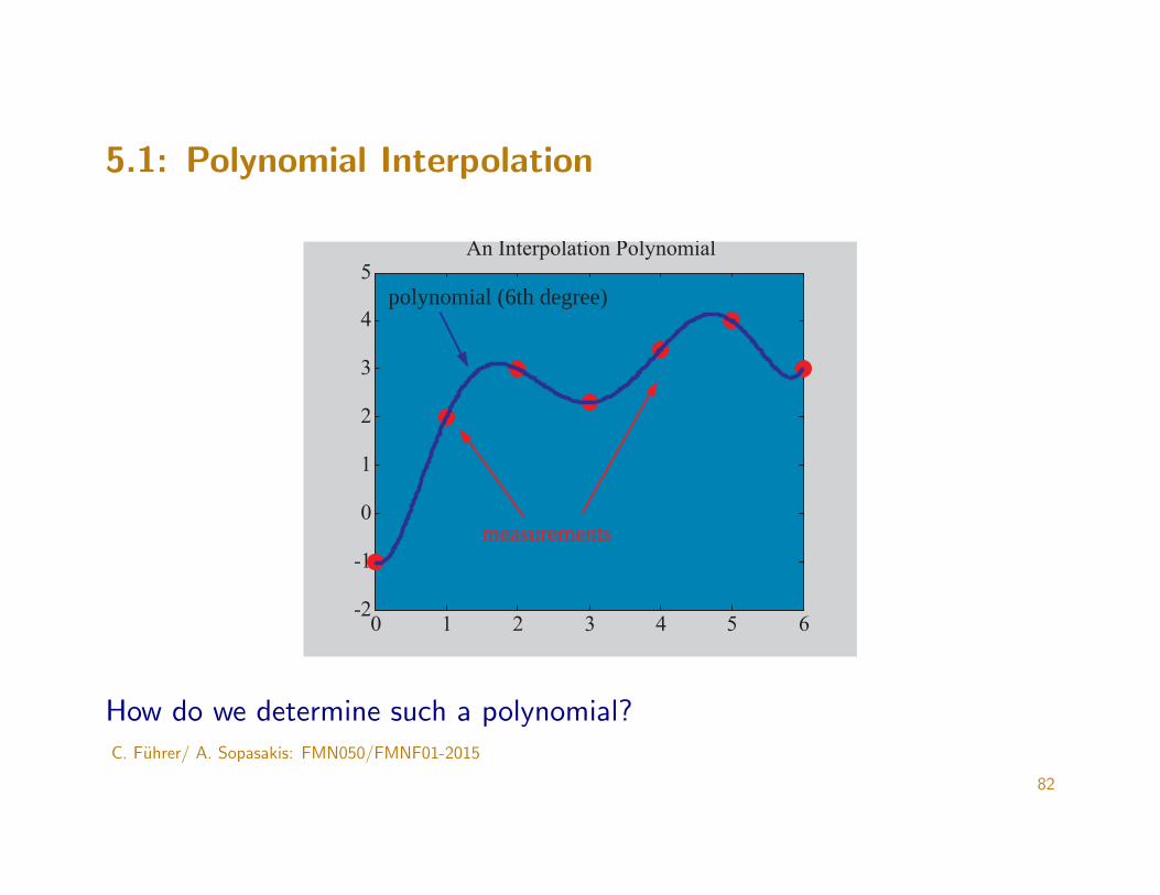
5An Interpolation Polynomial
measurements
polynomial (6th degree)
How do we determine such a polynomial?C. Fuhrer/ A. Sopasakis: FMN050/FMNF01-2015
82
5.2: Vandermonde Approach
Ansats: p(x) = anxn + an−1x
n−1 + · · · a1x+ a0
Interpolation conditionsp(xj) = anx
ni + an−1x
n−1i + · · · a1xi + a0 = yi 0 ≤ i ≤ n
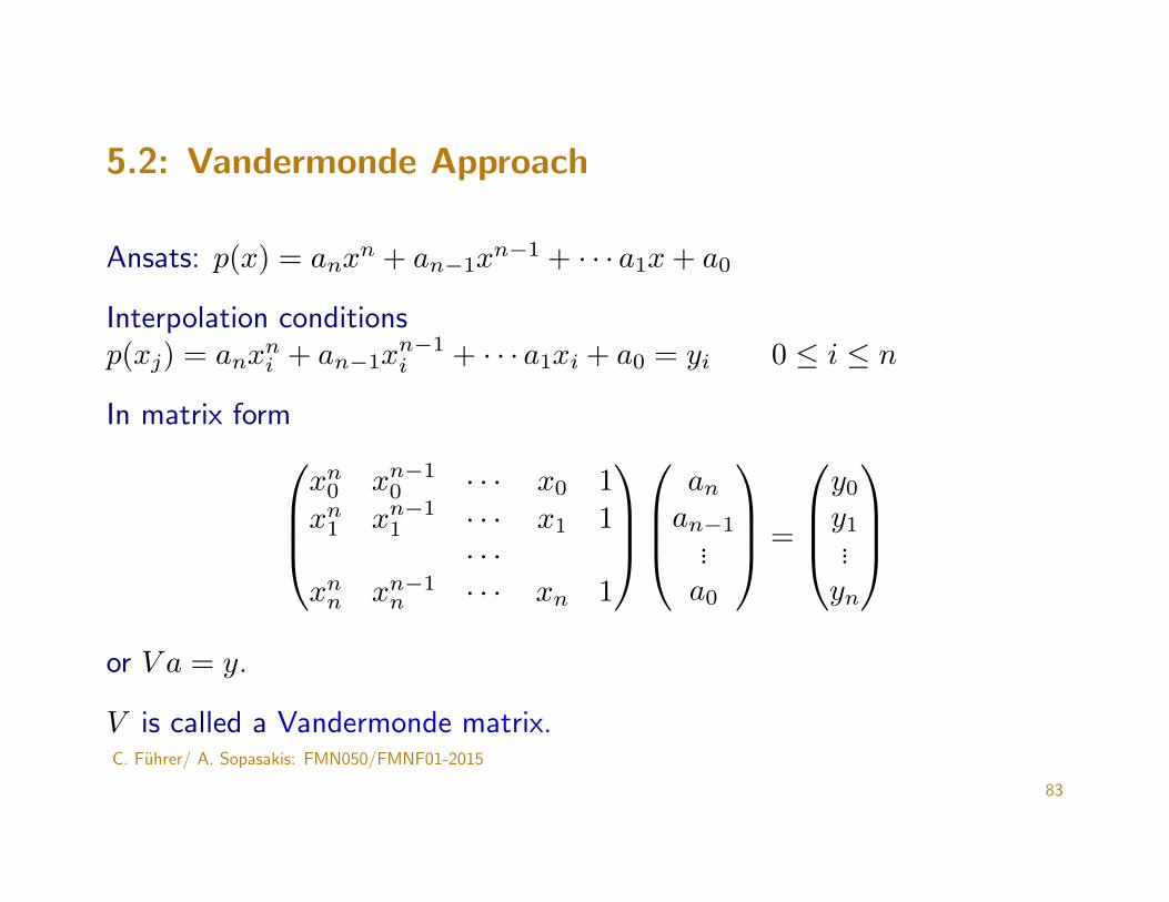
In matrix formxn0 xn−1
0 · · · x0 1xn1 xn−1
1 · · · x1 1· · ·
xnn xn−1n · · · xn 1
anan−1
...a0
=
y0
y1...yn
or V a = y.
V is called a Vandermonde matrix.C. Fuhrer/ A. Sopasakis: FMN050/FMNF01-2015
83
5.3 Vandermonde approach in MATLAB
polyfit sets up V and solves for a (the coefficients)
Alternatively vander sets up V and a = solve(V, y) solves for a.
polyval evaluates the polynomial for given x values.
n+ 1 points determine a polynomial of (max-)degree n.
Obs! n is input to polyfit .
C. Fuhrer/ A. Sopasakis: FMN050/FMNF01-2015
84
5.4 Vandermonde approach in MATLAB or Python
Essential steps to generate and plot an interpolation polynomial:
• Computing the coefficients (polyfit, vander etc)
• Generating x-values for ploting, e.g.xval=linspace(0,100,1000)
• Evaluating the polynomial, e.g. yval=polyval(coeff,xval)
• Plotting, e.g. plot(xval,yval).
C. Fuhrer/ A. Sopasakis: FMN050/FMNF01-2015
85
5.5 Lagrange Polynomials
We take now another approach to compute the interpolation polynomial
Definition. [–] The polynomials Li ∈ Pn with the property
Li(xj) =
{0 if i 6= j1 if i = j
are called Lagrange polynomials.
C. Fuhrer/ A. Sopasakis: FMN050/FMNF01-2015
86
5.6 Lagrange Polynomials (Cont.)
It is easy to check, that
Li(x) =
n∏j = 0i 6= j
(x− xj)(xi − xj)
The interpolation polynomial p can be written as
p(x) =
n∑i=0
yiLi(x)
Check that it indeed fulfils the interpolation conditions!C. Fuhrer/ A. Sopasakis: FMN050/FMNF01-2015
87
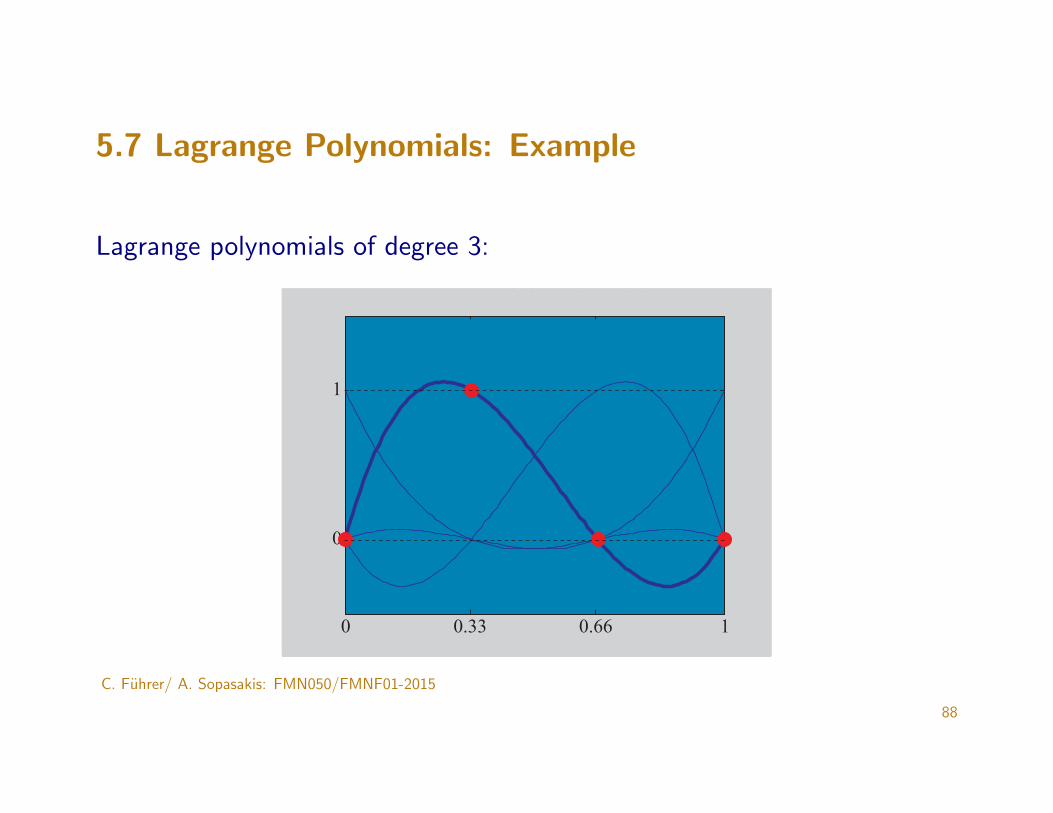
5.7 Lagrange Polynomials: Example
Lagrange polynomials of degree 3:
0 1 2 3 4 5 6-2
-1
0
1
2
3
4
5An Interpolation Polynomial
measurements
polynomial (6th degree)
0 0.33 0.66 1
0
1
C. Fuhrer/ A. Sopasakis: FMN050/FMNF01-2015
88
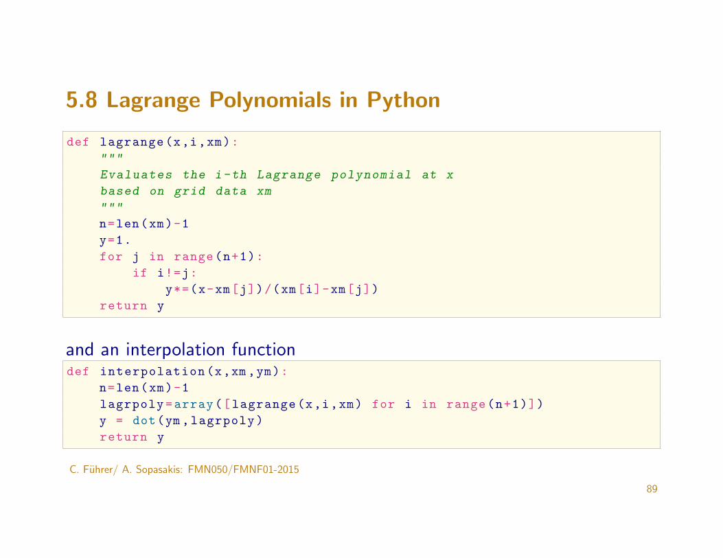
5.8 Lagrange Polynomials in Python
def lagrange(x,i,xm):
"""
Evaluates the i-th Lagrange polynomial at x
based on grid data xm
"""
n=len(xm)-1
y=1.
for j in range(n+1):
if i!=j:
y*=(x-xm[j])/(xm[i]-xm[j])
return y
and an interpolation functiondef interpolation(x,xm ,ym):
n=len(xm)-1
lagrpoly=array([lagrange(x,i,xm) for i in range(n+1)])
y = dot(ym ,lagrpoly)
return y
C. Fuhrer/ A. Sopasakis: FMN050/FMNF01-2015
89
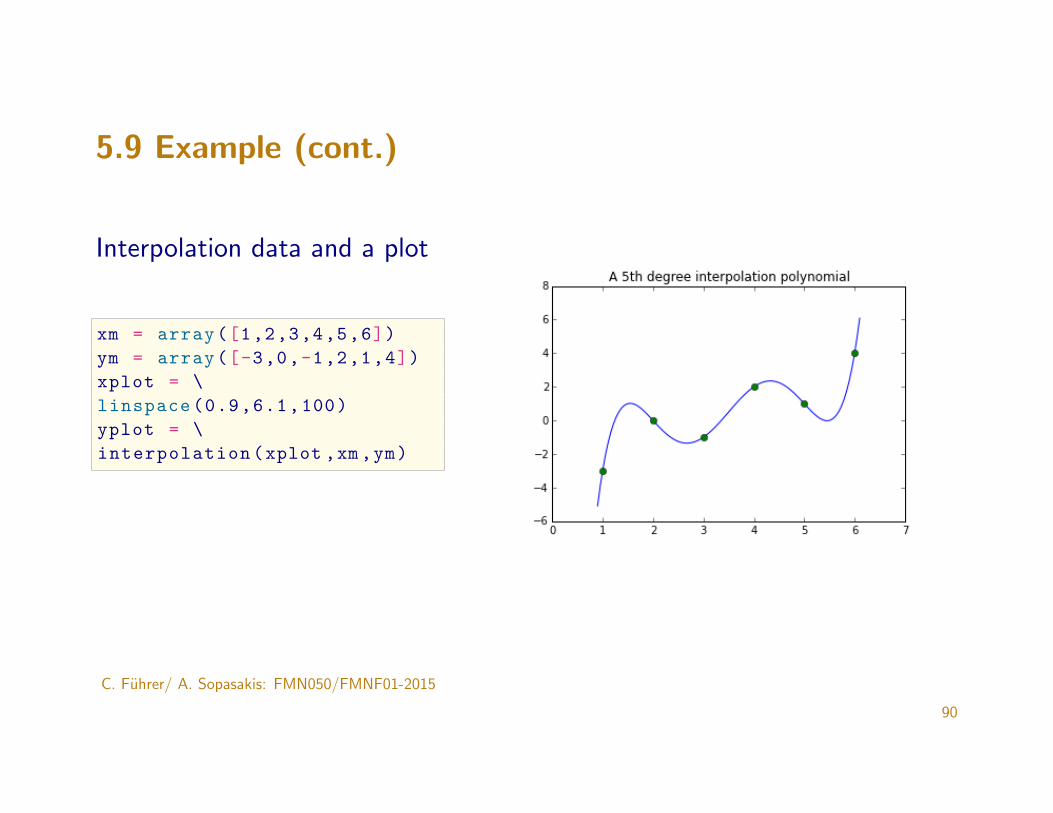
5.9 Example (cont.)
Interpolation data and a plot
xm = array([1,2,3,4,5,6])
ym = array([-3,0,-1,2,1,4])
xplot = \
linspace(0.9,6.1,100)
yplot = \
interpolation(xplot ,xm,ym)
C. Fuhrer/ A. Sopasakis: FMN050/FMNF01-2015
90
5.10 The vector space Pn
We have two ways to express a polynomial
Monomial representation p(x) =∑nk=0 akx
k
Lagrange representation p(x) =∑nk=0 ykL
nk(x)
They describe the same polynomial (as the interpolation polynomial isunique).
C. Fuhrer/ A. Sopasakis: FMN050/FMNF01-2015
91
5.11 The vector space Pn (Cont.)
We introduced two bases in Pn:
Monomial basis {1, x, x2, · · · , xn}, coordinates ak, k = 0 : n
Lagrange basis {Ln0 (x), Ln1 (x), · · · , Lnn(x)}, coordinates yk, k = 0 : n
It is easy to show, that these really are bases (linear independent elements).
C. Fuhrer/ A. Sopasakis: FMN050/FMNF01-2015
92