uniformly attracting solutions of nonautonomous ...aberger/papers/uniform... · uniformly...

Nonlinear Analysis 68 (2008) 3789–3811www.elsevier.com/locate/na

Uniformly attracting solutions of nonautonomousdifferential equations

A. Bergera,1, S. Siegmundb,∗

a Department of Mathematics and Statistics, University of Canterbury, Christchurch, New Zealandb Fachbereich Mathematik, Johann Wolfgang Goethe-Universitat, Frankfurt am Main, Germany

Received 5 February 2007; accepted 19 April 2007

Abstract

Understanding the structure of attractors is fundamental in nonautonomous stability and bifurcation theory. By means ofclarifying theorems and carefully designed examples we highlight the potential complexity of attractors for nonautonomousdifferential equations that are as close to autonomous equations as possible. We introduce and study bounded uniform attractors andrepellors for nonautonomous scalar differential equations, in particular for asymptotically autonomous, polynomial, and periodicequations. Our results suggest that uniformly attracting or repelling solutions are the true analogues of attracting or repelling fixedpoints of autonomous systems. We provide sharp conditions for the autonomous structure to break up and give way to a bewilderingdiversity of nonautonomous bifurcations.c© 2007 Elsevier Ltd. All rights reserved.

MSC: primary 34A12; 34D45; 37C70; secondary 34C07; 34C11; 37B55

Keywords: Nonautonomous dynamical system; Attractor; Repellor; Asymptotically autonomous; Polynomial differential equation; Poincare map

1. Introduction

From the plethora of tools for analysing the asymptotic behaviour of autonomous differential equations

x = F(x), (1)

many have been extended to nonautonomous equations

x = f (t, x), (1)t

e.g. spectral theory [38,42], invariant manifold theory [3,48], or the Hartman–Grobman theorem [4,34,43]. As animportant common feature, all these generalisations assume uniformity in time t ∈ R of some sort or other, for instancevia exponential dichotomies of a linearisation or via Lipschitz conditions independent of t . Imposing uniformity

∗ Corresponding author. Tel.: +49 69 798 22517; fax: +49 69 798 28846.E-mail addresses: [email protected] (A. Berger), [email protected] (S. Siegmund).

1 Tel.: +64 3 364 2682; fax: +64 3 364 2587.

0362-546X/$ - see front matter c© 2007 Elsevier Ltd. All rights reserved.doi:10.1016/j.na.2007.04.020

http://www.elsevier.com/locate/na

mailto:[email protected]

mailto:[email protected]

http://dx.doi.org/10.1016/j.na.2007.04.020

3790 A. Berger, S. Siegmund / Nonlinear Analysis 68 (2008) 3789–3811

conditions is reasonable if a priori knowledge on the time dependence of f is available, e.g. if f is periodic,almost periodic or automorphic in t [41], but it may become questionable if the dependence on t is more complex.For a comprehensive study of bifurcation scenarios for instance an analysis of more general time dependencies isindispensable.

The recent past has seen numerous attempts to extend bifurcation theory to nonautonomous differential equations[9,13,16–19,22,25,27,28,36]. While classical bifurcation theory for dynamical systems (1) describes the change ofstability and the creation, annihilation and break up of equilibria, periodic, heteroclinic and homoclinic orbits etc., it is,in the nonautonomous situation of (1)t, not at all obvious the bifurcations of which objects one should study; equilibriaand periodic orbits for instance are not generic for (1)t if f depends aperiodically on t . One natural approach is tostudy the transition of attractors [25]. For example, a classical (supercritical) two-dimensional Hopf bifurcation couldbe understood as a transition from a singleton attractor (consisting of an asymptotically stable equilibrium) to a morecomplex attractor (bounded by an attractive periodic orbit and containing in its interior a repelling equilibrium). Whilea classical attractor for (1) is simply a compact invariant set which attracts a neighbourhood, there exist several non-equivalent definitions for nonautonomous attractors, e.g. forward and pullback attractors [6] describing, respectively,the future and the past of (1)t. Consequently, in order to better understand nonautonomous bifurcation scenarios onehas to analyse the structure and transition of these attractors whenever Eq. (1)t depends on a parameter. Typically,attractors depend merely upper semi-continuously on parameters; the dependence is continuous only if the attractionis uniform w.r.t. the parameter [29]. Clearly, establishing the existence of some (globally) attracting object can onlybe the first step of an in-depth analysis. Looking inside an attractor, however, usually is much more demanding. Tothe best of our knowledge no systematic study of internal attractor bifurcations for nonautonomous equations existsso far. Bifurcation results available often rely on the fact that attracting solutions can be computed and analysedexplicitly [25,27] or employ somewhat technical or restrictive assumptions on the system under consideration, as forinstance in the formidable balance of Taylor coefficients utilised in [28].

The purpose of this article is to lay the foundations for internal attractor bifurcation studies. In the simplestpossible setting we illustrate by means of clarifying theorems and carefully designed examples the potential structuralcomplexity of attractors for equations which are as close to autonomous differential equations as possible. We studyattraction and repulsion properties of individual solutions (i.e., the natural analogues of autonomous equilibria) ofnonautonomous scalar differential equation (1)t. In Section 2 we propose the definition of a bounded uniform attractorwhich incorporates two of the most popular mechanisms of attraction, namely forward and pullback attraction. In theautonomous situation of (1), all notions of attraction coincide. In general, a uniform attractor for (1)t is substantiallymore than just a forward attractor that is also pullback attracting (see Examples 5 and 12); as far as we know, thisimportant point has not been clarified in the literature before. In Section 3 we study in detail the properties of uniformattractors and repellors for nonautonomous equation (1)t where we maintain various autonomous features by focusingon equations that are, respectively, asymptotically autonomous (Section 3.1), polynomial in x (Section 3.2), andperiodic in t (Section 3.3). While all notions of attraction coincide for scalar periodic equations (Theorem 23), ingeneral the classes of forward, pullback, and uniform attractors are all different, the latter being strictly smaller thanthe intersection of the two former.

From Section 3.2 onward, we pay special attention to uniform attractors and repellors of Eq. (1)t that arepolynomial in x ,

x = ε(

a0(t)+ a1(t)x + · · · + ad(t)xd)

(2)

with ε > 0. In the autonomous case, that is, for a0, a1, . . . , ad not depending on t , the total number of uniformlyattracting and repelling solutions of (2) is, quite trivially, bounded by d. The latter bound turns out to be correct aswell if either (2) is asymptotically autonomous, if ε > 0 is sufficiently small, or if d ≤ 3, where in the case d = 3additional assumptions have to be imposed on a3 (see Theorem 21 for details). Quite different arguments are requiredto deal with each situation. Moreover, none of the assumptions mentioned can be omitted. We demonstrate this bymeans of a series of results which unite and profoundly extend ideas scattered throughout the literature. To give butone example, even for periodic coefficients ai Eq. (2) may have any (finite) number of uniform attractors if d ≥ 3 —provided that ε is not too small (Theorem 28). Thus a non-trivial bifurcation problem emerges for (2) upon variation ofε. Our results strongly suggest that the notion of uniform attractors and repellors will be useful in tackling problems of

A. Berger, S. Siegmund / Nonlinear Analysis 68 (2008) 3789–3811 3791

this kind. Accordingly, we conclude this article by indicating several fundamental questions that arise naturally fromthe results presented.

2. Bounded uniform attractors and repellors

In this article we consider nonautonomous scalar differential equations

x = f (t, x), (3)

where f : R2→ R as well as ∂

∂x f is continuous in (t, x). Moreover, we assume throughout that supR×K | f | < ∞

for every compact set K ⊂ R. Given (t0, x0) ∈ R2 the initial value problem consisting of (3) together with x(t0) = x0has a unique solution t 7→ ϕ(t; t0, x0) defined on some (possibly bounded) maximal open interval containing t0.Although solutions of (3) may (and often will) become unbounded in finite time we are particularly interested inbounded solutions. A bounded solution µ : R → R of (3) can attract or repel neighbouring solutions in differentways.

Example 1. Let ψ denote the bounded C1 function

ψ : t 7→t |t |

1 + t2 (t ∈ R),

which, together with its primitive

Ψ : t 7→

∫ t

0ψ(s)ds = |t | − |arctan t | (t ∈ R),

will be used several times throughout this article as an auxiliary function. With this, consider the equation

x = cos t + ψ(t) sin t − ψ(t)x, (4)

which, for all (t0, x0) ∈ R2, has the solution

ϕ(t; t0, x0) = eΨ (t0)−Ψ (t)(x0 − sin t0)+ sin t.

Obviously, all solutions of (4) exist for all time, every solution is bounded, and

limt→∞

|ϕ(t; t0, x0)− sin t | = 0, ∀(t0, x0) ∈ R2. (5)

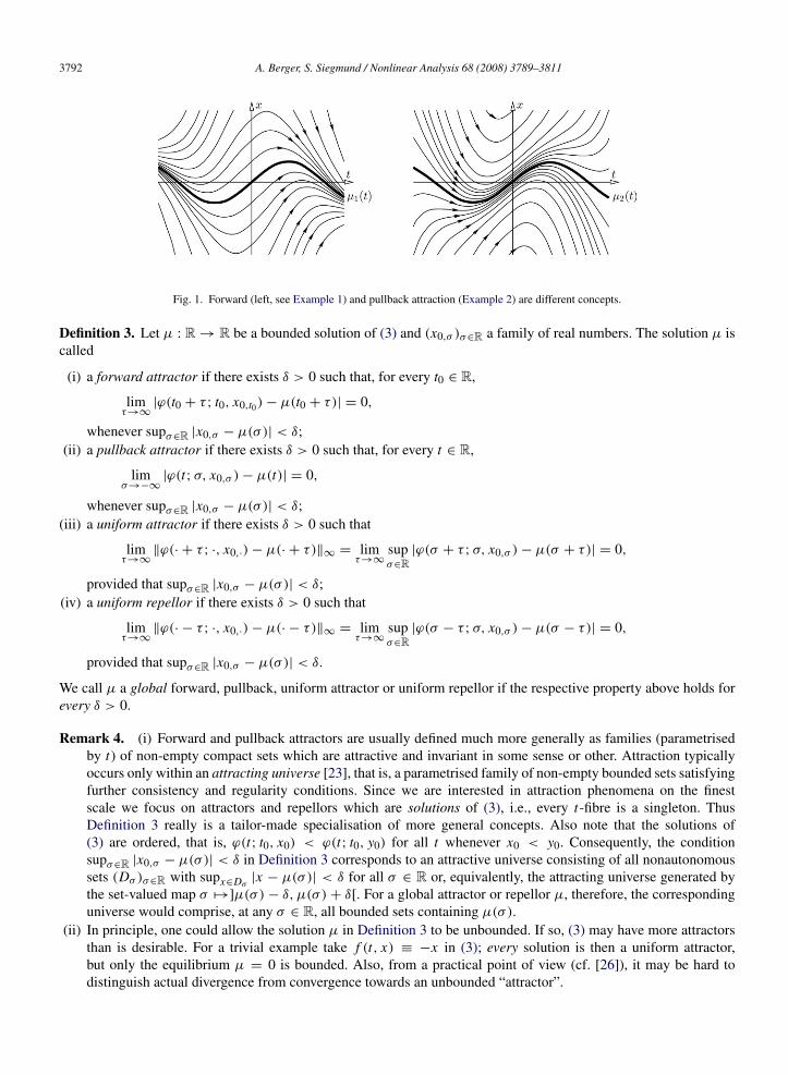
Thus the bounded solution µ1 : t 7→ sin t of (4) attracts all solutions in forward time (see Fig. 1). It is an example ofa (global) forward attractor.

Example 2. Analogously, for the equation

x = cos t − ψ(t) sin t + ψ(t)x, (6)

we find, for all (t0, x0) ∈ R2,

ϕ(t; t0, x0) = eΨ (t)−Ψ (t0)(x0 − sin t0)+ sin t.

Now µ2 : t 7→ sin t is the only bounded solution of (6). Evidently, it is not attracting in the sense of the previousexample (see Fig. 1). However, µ2 attracts all solutions in the sense that, at any given time t , solutions satisfying aninitial condition at time t0 much smaller than t are close to µ2(t). Formally

limt0→−∞

|ϕ(t; t0, x0)− sin t | = 0, ∀t ∈ R, x0 ∈ R. (7)

Thus µ2 is an example of a (global) pullback attractor.

It is obvious that µ1 is not pullback attracting for (4) whereas µ2 is not forward attracting for (6). Evidently, thisdiscrepancy is due to the highly non-uniform convergence in (5) and (7). Observations like these naturally motivateparts (iii) and (iv) of Definition 3. This definition may look slightly unfamiliar to the reader proficient in the theoryof nonautonomous attractors, as developed e.g. in [7,8,23,24]. The subsequent Remark 4 explicates why Definition 3nevertheless is the most appropriate for our purposes.


Fig. 1. Forward (left, see Example 1) and pullback attraction (Example 2) are different concepts.

Definition 3. Let µ : R → R be a bounded solution of (3) and (x0,σ )σ∈R a family of real numbers. The solution µ iscalled

(i) a forward attractor if there exists δ > 0 such that, for every t0 ∈ R,

limτ→∞

|ϕ(t0 + τ ; t0, x0,t0)− µ(t0 + τ)| = 0,

whenever supσ∈R |x0,σ − µ(σ)| < δ;(ii) a pullback attractor if there exists δ > 0 such that, for every t ∈ R,

limσ→−∞

|ϕ(t; σ, x0,σ )− µ(t)| = 0,

whenever supσ∈R |x0,σ − µ(σ)| < δ;(iii) a uniform attractor if there exists δ > 0 such that

limτ→∞

‖ϕ(· + τ ; ·, x0,·)− µ(· + τ)‖∞ = limτ→∞

supσ∈R

|ϕ(σ + τ ; σ, x0,σ )− µ(σ + τ)| = 0,

provided that supσ∈R |x0,σ − µ(σ)| < δ;(iv) a uniform repellor if there exists δ > 0 such that

limτ→∞

‖ϕ(· − τ ; ·, x0,·)− µ(· − τ)‖∞ = limτ→∞

supσ∈R

|ϕ(σ − τ ; σ, x0,σ )− µ(σ − τ)| = 0,

provided that supσ∈R |x0,σ − µ(σ)| < δ.

We call µ a global forward, pullback, uniform attractor or uniform repellor if the respective property above holds forevery δ > 0.

Remark 4. (i) Forward and pullback attractors are usually defined much more generally as families (parametrisedby t) of non-empty compact sets which are attractive and invariant in some sense or other. Attraction typicallyoccurs only within an attracting universe [23], that is, a parametrised family of non-empty bounded sets satisfyingfurther consistency and regularity conditions. Since we are interested in attraction phenomena on the finestscale we focus on attractors and repellors which are solutions of (3), i.e., every t-fibre is a singleton. ThusDefinition 3 really is a tailor-made specialisation of more general concepts. Also note that the solutions of(3) are ordered, that is, ϕ(t; t0, x0) < ϕ(t; t0, y0) for all t whenever x0 < y0. Consequently, the conditionsupσ∈R |x0,σ − µ(σ)| < δ in Definition 3 corresponds to an attractive universe consisting of all nonautonomoussets (Dσ )σ∈R with supx∈Dσ |x − µ(σ)| < δ for all σ ∈ R or, equivalently, the attracting universe generated bythe set-valued map σ 7→]µ(σ)− δ, µ(σ )+ δ[. For a global attractor or repellor µ, therefore, the correspondinguniverse would comprise, at any σ ∈ R, all bounded sets containing µ(σ).

(ii) In principle, one could allow the solution µ in Definition 3 to be unbounded. If so, (3) may have more attractorsthan is desirable. For a trivial example take f (t, x) ≡ −x in (3); every solution is then a uniform attractor,but only the equilibrium µ = 0 is bounded. Also, from a practical point of view (cf. [26]), it may be hard todistinguish actual divergence from convergence towards an unbounded “attractor”.


(iii) The notions of uniform attractor and repellor exhibit a natural duality. Such natural dual counterparts exist neitherfor forward nor for pullback attractors [6,21,25,27].

Example 5. Trivially, every uniform attractor is both a forward and a pullback attractor. The converse is not true ingeneral as the following example shows.

For every a ∈ R let ha denote the bounded continuous function

ha : t 7→ 1 − a − π max(

0, sin√

|t |)

(t ∈ R),

and consider the equation

x = cos t − ha(t) sin t + ha(t)x, (8)

for which a short computation yields

ϕ(t; t0, x0) = (x0 − sin t0)e∫ t

t0ha(s)ds

+ sin t ∀(t0, x0) ∈ R2. (9)

Since ha is even, the solution µ : t 7→ sin t of (8) is a forward attractor if and only if it is a pullback attractor,which in turn is the case precisely if a > 0. On the other hand, given any τ > 0, pick N ∈ N such that(2N + 1)2π2

+ τ < (2N + 2)2π2, that is, N > 14π

−2(τ − 3π2). Choosing in particular t0 = (2N + 1)2π2 weimmediately deduce from (9) that

supσ∈R

|ϕ(σ + τ ; σ, x0,σ )− sin(σ + τ)| ≥ |x0 − sin t0|eτ(1−a).

Thus µ is not a uniform attractor if a ≤ 1. For a > 1 obviously ha ≤ 1 − a < 0, so

supσ∈R

|ϕ(σ + τ ; σ, x0,σ )− sin(σ + τ)| ≤ eτ(1−a) supσ∈R

|x0,σ − sin σ | → 0 as τ → ∞,

which shows that µ is a global uniform attractor if and only if a > 1.

Example 6. Two bounded solutions µ1, µ2 of (3) may be separated in the sense that their distance inft∈R |µ1(t) −

µ2(t)| is positive. Any uniform attractor is necessarily separated from any uniform repellor (cf. the proof ofTheorem 19). It is, however, worth noting that limt→∞ |µ1(t) − µ2(t)| = 0 for two uniform attractors µ1, µ2 isnot ruled out by Definition 3. Concretely, consider the equation

x =12(1 − ψ(t)) x −

12

x3, (10)

the solutions of which are given by

ϕ(t; t0, x0) =x0√

eΨ (t)−t−Ψ (t0)+t0 + x20

∫ tt0

eΨ (t)−t−Ψ (s)+sds∀(t0, x0) ∈ R2, t ≥ t0. (11)

Taking the limit t0 → −∞ in (11) yields two candidates for pullback attractors for (10), namely µ and −µ, where

µ : t 7→1√∫ t

−∞eΨ (t)−t−Ψ (s)+sds

(t ∈ R).

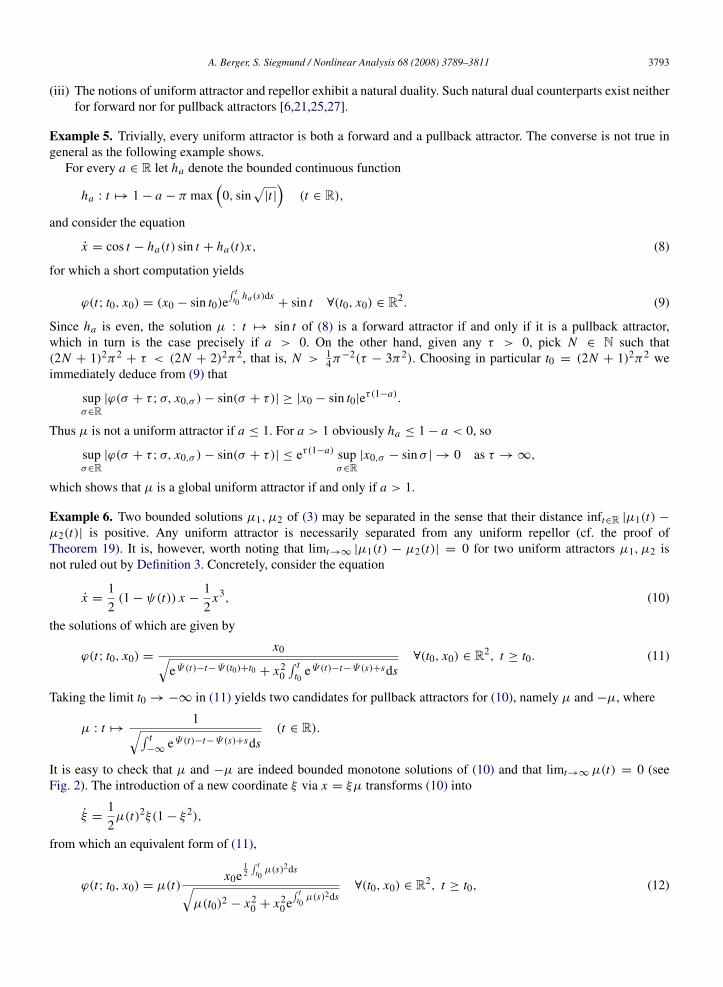
It is easy to check that µ and −µ are indeed bounded monotone solutions of (10) and that limt→∞ µ(t) = 0 (seeFig. 2). The introduction of a new coordinate ξ via x = ξµ transforms (10) into

ξ =12µ(t)2ξ(1 − ξ2),

from which an equivalent form of (11),

ϕ(t; t0, x0) = µ(t)x0e

12

∫ tt0µ(s)2ds√

µ(t0)2 − x20 + x2

0 e∫ t

t0µ(s)2ds

∀(t0, x0) ∈ R2, t ≥ t0, (12)


Fig. 2. The two uniform attractors µ and −µ of (10) are not separated.

can be derived easily. The representation (12) is particularly useful for showing that µ and −µ are in fact uniformattractors of (10). Since limt→∞ |µ(t)− (−µ(t)) | = 0 these two attractors are evidently not separated.

From Theorem 13 it follows that limt→−∞ µ(t) =√

2. This theorem also implies that the zero solution of (10)which in Fig. 2 appears somewhat repelling is not a uniform repellor; while it is not a uniform attractor either, it isobviously a forward attractor.

Example 7. To observe an infinite number of attractors that are not separated consider

x = −et (1 + et )−1x + (1 + et )−1 H(x(1 + et )

), (13)

where H denotes the C∞ function

H(x) =

{0 if x = 0,

e−|x |−1

sin(x−1) if x 6= 0.

For every k ∈ Z \ {0} the function

µk : t 7→1

kπ(1 + et )−1 (t ∈ R),

is a solution of (13). As in Example 6 it is straightforward to check that µk is a uniform attractor whenever k is even.Note also that for odd k the solution µk , albeit somewhat repelling, is not a uniform repellor but – like every solutionof (13) – a forward attractor.

The following simple fact implicitly underlies most of the subsequent arguments, and we recall it here for thereader’s convenience, see e.g. [47].

Proposition 8. Let µ1 < µ2 be two bounded solutions of (3). Then the solution of (3) with x(t0) = x0 exists for allt ∈ R whenever µ1(t0) ≤ x0 ≤ µ2(t0).

3. Properties of uniform attractors

A uniform attractor resembles an attracting equilibrium in the autonomous case. We now analyse analogies anddifferences between the two concepts. Recall that throughout we assume f in (3), and also ∂

∂x f , to be continuous in(t, x) and bounded on every stripe R × K , K compact.

3.1. Autonomous and asymptotically autonomous differential equations

In the autonomous case, that is for f (t, x) ≡ F(x) not depending on t , all notions of attraction coincide, andattractors are easily characterised in terms of F . Essentially, this is due to the invariance of (1) under time translations.

Theorem 9. Let F be C1 and µ : R → R a bounded solution of x = F(x). Then the following statements areequivalent:


(i) µ is a forward attractor;(ii) µ is a pullback attractor;

(iii) µ is a uniform attractor;(iv) µ is constant, µ(t) ≡ µ0, and µ0 is an isolated zero of F such that F(a) > 0 > F(b) for all a < µ0 < b with

b − a sufficiently small.

Proof. Current as well as later arguments become especially transparent by means of α- and ω-limit sets and theirnonautonomous counterparts [15,33]. Quite generally, therefore, for every bounded continuous function ν : R → Rwe denote by α(ν) and ω(ν) the set of all backward and forward accumulation points of {ν(t) : t ∈ R}, respectively,i.e.,

α(ν) = {x ∈ R : ∃(tn) s.t. tn → ∞, ν(−tn) → x},

ω(ν) = {x ∈ R : ∃(tn) s.t. tn → ∞, ν(tn) → x}.

It is well known (and easy to see) that α(ν), ω(ν) are non-empty compact intervals (which may, of course, degenerateto single points).

Every solution µ of x = F(x) is monotonic, and therefore the limits limt→−∞ µ(t) = µ− and limt→∞ µ(t) = µ+

exist if µ is bounded. Thus α(µ) = {µ−} and ω(µ) = {µ+}. Clearly, F(µ−) = F(µ+) = 0. Assume now that µ is aforward attractor. If µ− 6= µ+ and δ > 0, then there exists t0 such that |µ− − µ(t0)| < δ yet

|ϕ(t0 + τ ; t0, µ−)− µ(t0 + τ)| = |µ− − µ(t0 + τ)| → |µ− − µ+| 6= 0 as τ → ∞,

contradicting the fact that µ is a forward attractor. Hence µ+ = µ− = µ0, and µ is constant. Similarly, if µ is apullback attractor then, for all σ ≤ t0 with t0 sufficiently small, |µ− − µ(σ)| < δ and so, choosing x0,σ equal to µ−

or µ(σ), depending on whether σ ≤ t0 or σ > t0, we find

limσ→−∞

|ϕ(t; σ, x0,σ )− µ(t)| = |µ− − µ(t)| 6= 0,

unless µ is constant. In either case therefore µ(t) ≡ µ0 and F(µ0) = 0. If there existed a strictly increasing sequence(an) with an → µ0 and F(an) ≤ 0 for all n then ϕ(t; t0, an) would neither converge to µ0 as t → ∞ nor ast0 → −∞. A completely analogous argument yields that F(b) < 0 for all b larger than but sufficiently close to µ0.Overall, this shows that (i) and (ii), and hence also (iii), imply (iv).

Conversely, assume that F(µ0) = 0 and F(a) > 0 > F(b) for all a, b with a0 ≤ a < µ0 < b ≤ b0and appropriate a0 < µ0 < b0. For every x0 ∈ [a0, b0] the solution ϕ(t; t0, x0) exists for all t ≥ t0, and, withδ = min(b0 − µ0, µ0 − a0) > 0,

supσ∈R

|ϕ(σ + τ ; σ, x0,σ )− µ0| = supσ∈R

|ϕ(τ ; 0, x0,σ )− µ0|

≤ max(|ϕ(τ ; 0, a0)− µ0|, |ϕ(τ ; 0, b0)− µ0|) → 0 as τ → ∞,

provided that supσ∈R |x0,σ − µ(σ)| < δ. Thus µ = µ0 is a uniform attractor. �

Corollary 10. Let F be C1 and µ : R → R a bounded solution of x = F(x). Then µ is a uniform repellor if andonly if µ(t) ≡ µ0 and µ0 is an isolated zero of F such that F(a) < 0 < F(b) for all a < µ0 < b with b − asufficiently small.

Proof. We only have to observe that µ is a uniform repellor if and only if t 7→ µ(−t) is a uniform attractor for theequation x = −F(x). �

Recall that (3) is termed asymptotically autonomous if for two (necessarily continuous) functions f−, f+ : R → R

limt→−∞

f (t, x) = f−(x), limt→∞

f (t, x) = f+(x),

holds locally uniformly in x . (See e.g. [33,44,45] for information and references on the extensive theory ofasymptotically autonomous systems; note that solutions of the limiting equations x = f−(x) and x = f+(x) may failto be unique if f−, f+ are not Lipschitz continuous.) In some respects, asymptotically autonomous systems resembleautonomous ones, but there are also various counterexamples to the intuition that the asymptotic behaviour of (3)and its limit equations x = f−(x), x = f+(x) are necessarily the same [45]. The latter point is emphasised by the


following example which shows that the equivalence of all notions of attraction, as established by Theorem 9 for theautonomous case, does not even extend to asymptotically autonomous systems.

Example 11. Let a0, a1 denote the bounded C1 functions

a0(t) = e−Ψ (t) and a1(t) = −1 − ψ(t) (t ∈ R),

respectively, with the functions ψ and Ψ introduced in Example 1, and consider the asymptotically autonomousequation

x = a0(t)+ a1(t)x, (14)

for which f−(x) ≡ 0 and f+(x) = −2x . An elementary computation confirms that

µ : t 7→ e−Ψ (t)= a0(t) (t ∈ R),

is a global forward but not a pullback attractor for (14).Similarly, choosing C1 functions a0, a1 as

a0(t) = eΨ (t)−t2(1 − 2t) and a1(t) = −1 + ψ(t) (t ∈ R),

yields another asymptotically autonomous equation (14) with f−(x) = −2x , f+(x) ≡ 0. In this case, the boundedsolution

µ : t 7→ eΨ (t)−t2(t ∈ R)

fails to be forward attracting but nevertheless is a global pullback attractor.

Example 12. In the setting of the previous example, let

a0(t) = e−t2(1 − 2t), a1(t) = |t |−

14 min

(0, sin

√|t |

)(t ∈ R).

Again, (14) is asymptotically autonomous with f+(x) = f−(x) ≡ 0. Define A1(t) =∫ t

0 a1(s)ds, t ∈ R. Then the C1

function

µ : t 7→

∫ t

−∞

a0(s)eA1(t)−A1(s)ds (t ∈ R),

is a bounded solution of (14) with lim|t |→∞ µ(t) = 0. It is easy to check that µ is both a global forward and pullbackattractor. An argument similar to the one in Example 5 shows that µ is not a uniform attractor, essentially because A1contains arbitrarily long constant sections.

Thus for asymptotically autonomous equations all concepts discussed so far are different. Nevertheless, for uniformattractors Theorem 9 in a sense extends to such equations.

Theorem 13. Assume (3) is asymptotically autonomous, and let µ : R → R be a uniform attractor. Then the limits

limt→−∞

µ(t) = µ−, limt→∞

µ(t) = µ+,

exist and satisfy f−(µ−) = f+(µ+) = 0. Moreover, for all a < µ+ < b with b − a sufficiently small,f+(a) ≥ 0 ≥ f+(b). Similarly, f−(c) ≥ 0 ≥ f−(d) for all c < µ− < d with d − c sufficiently small. Furthermore,f− and f+ do not vanish identically on any neighbourhood of µ− and µ+, respectively.

Proof. We only prove the assertions concerning f+ and µ+ because the arguments for backward time are completelyanalogous. Assume that µ is a uniform attractor and let ω(µ) = [ω1, ω2]. Since lim inft→∞ µ(t) would be smaller orlarger than ω1 if f+(ω1) were, respectively, negative or positive, we must have f+(ω1) = 0, and in fact f+(x) = 0for every x ∈ ω(µ).

Assume now that ω1 < ω2 and define a(t) = supx∈ω(µ) | f (t, x)|, t ∈ R, as well as c =23ω1+

13ω2, d =

13ω1+

23ω2.

We can find a strictly increasing sequence (sn) with sn → ∞ such that, for all n ∈ N, µ([sn, sn + n]) ⊂ [c, d] and

supt≥sna(t) < 1

6 (ω2 − ω1)/n, but also∫ sn+n

sna(s)ds → 0 as n → ∞. Given δ > 0, let δ′ = min

(δ, 1

6 (ω2 − ω1))


and assume that |x0 − µ(sn)| < δ′. Then both µ(t) and ϕ(t; sn, x0) are contained in ω(µ) for all sn ≤ t ≤ sn + n.Assuming without loss of generality that

∫ sn+nsn

a(s)ds < 18δ

′ for all n and that µ(sn) > x0, we deduce from the trivialestimate

µ(t)− ϕ(t; sn, x0) ≥ µ(sn)− x0 − 2∫ t

sn

a(s)ds ∀t ∈ [sn, sn + n],

that µ(t) − ϕ(t; sn, x0) ≥ |µ(sn) − x0| −14δ

′ for all t ∈ [sn, sn + n]. Let x0,σ = µ(sn) −12δ

′ if σ = sn for some n,and x0,σ = µ(σ) otherwise. Then µ(t)− ϕ(t; sn, x0,sn ) ≥

14δ

′ for all t ∈ [sn, sn + n] and therefore

lim supτ→∞

supσ∈R

|ϕ(σ + τ ; σ, x0,σ )− µ(σ + τ)| ≥14δ′,

while ‖x0,· − µ(·)‖∞ < δ′. This contradicts the fact that µ is a uniform attractor. Consequently, ω1 = ω2 = µ+.The preceding arguments also show that f+ cannot vanish identically on any neighbourhood of µ+. Finally, if

f+(an) < 0 for all n ∈ N and some increasing sequence (an) with an → µ+ then, for t0 sufficiently large, ϕ(t; t0, an)

does not converge to µ+ as t → ∞, which clearly contradicts the fact that µ is an attractor. �

Corollary 14. If µ is a uniform repellor of the asymptotically autonomous equation x = f (t, x) then the limitslimt→−∞ µ(t) = µ−, limt→∞ µ(t) = µ+ exist and satisfy f−(µ−) = f+(µ+) = 0. For all a < µ+ < b with b − asufficiently small, f+(a) ≤ 0 ≤ f+(b), and for all c < µ− < d with d − c sufficiently small, f−(c) ≤ 0 ≤ f−(d).Also, f− and f+ do not vanish identically on any neighbourhood of µ− and µ+, respectively.

Example 15. Theorem 13 and Corollary 14 should be seen as extensions of, respectively, Theorem 9 and Corollary 10to asymptotically autonomous equations and their uniform attractors. An analogous statement for forward or pullbackattractors is false. For example, the equation

x =4√

2t2|t |

1 + t4 cos(

log(1 + t4))

−4t2

|t |

1 + t4 x

is asymptotically autonomous, with f+ = f− = 0, and has

µ : t 7→ sin(π

4+ sign t · log(1 + t4)

)(t ∈ R)

as a global forward and pullback attractor. (Here, as usual, sign t equals 1, 0 or −1, depending on whether t ∈ R ispositive, zero or negative.) It follows from Theorem 13 that µ is not a uniform attractor; this can also be confirmed bya short direct computation.

Example 16. Unlike Theorem 9 for the autonomous case, Theorem 13 does not assert that µ+ is an isolated zero off+. In general, this cannot be expected as the following example shows.

Define f : R2→ R as

f (t, x) =

0 if x = 0,

−xe−|x |−1

((1 + e−t2

sign x) sin2(x−1)+ e−t2) 1

4if x 6= 0,

so that f is C∞ in t and x , and f (t, x) → f±(x) locally uniformly as |t | → ∞, where

f±(x) =

{0 if x = 0,

−xe−|x |−1

| sin(x−1)|12 if x 6= 0.

Obviously, µ = 0 is a solution of x = f (t, x). As before let t 7→ ϕ(t; t0, x0) denote the (unique) solution of the latterequation with x(t0) = x0. Furthermore, let w be any solution of the autonomous initial value problem

w = f±(w), w(0) = x0. (15)

As ( f+(x)− f (t, x)) sign x ≥ 0 for all (t, x) ∈ R2 it follows from elementary differential inequalityconsiderations [47, p. 95] that (w(t − t0)− ϕ(t; t0, x0)) sign x0 ≥ 0 for all t ≥ t0. Choosing in particular w as


the minimal solution of (15) if x0 > 0, and as the maximal solution if x0 < 0, we see that µ is indeed a uniformattractor, but clearly µ+ = 0 is not an isolated zero of f±.

Example 16 is somewhat pathological in that (15) does not have a unique solution. An additional regularityassumption on the limiting functions simplifies the situation.

Theorem 17. If, under the assumptions of Theorem 13, the functions f− and f+ are C1 then µ− and µ+ are isolatedzeros of f− and f+, respectively.

Proof. Again it is enough to verify the assertion for forward time. Assume that f+(µn) = 0 for all n ∈ N and somemonotone sequence (µn) with µn → µ+; without loss of generality let (µn) be strictly decreasing. We are going toshow that this assumption is incompatible with µ being a uniform attractor — provided that f+ is C1.

If f ′+(µn) 6= 0 for infinitely many n then there exist points x > µ+ with x − µ+ > 0 arbitrarily small such that

f (t, x) is positive for all sufficiently large t . This, however, is impossible because µ is an attractor. Without loss ofgenerality we can thus assume that f ′

+(µn) = 0 for all n ∈ N. Given δ > 0, choose N ∈ N such that |µ(t)−µN | < δ

for all t ≥ N . For every k ∈ N there exists 0 < εk <13 (µN − µ+) such that | f ′

+(x)| <1

2k whenever |x − µN | < εk .Consequently, we can find a strictly increasing sequence (Tk)k∈N with T1 > N such that | f (t, x)| < εk

k for all t ≥ Tk

and all x ∈ [µN − εk, µN + εk], and also µ(t) < 23µ+ +

13µN whenever t ≥ T1. It follows that ϕ(t; Tk, µN ) is an

element of [µN − εk, µN + εk] for (at least) all t ∈ [Tk, Tk + k]. Choose now x0,σ = µN if σ = Tk for some k, andx0,σ = µ(σ) otherwise. Clearly, supσ∈R |x0,σ − µ(σ)| < δ. Observing that

supσ∈R

|ϕ(σ + τ ; σ, x0,σ )− µ(σ + τ)| ≥ |ϕ(Tk + τ ; Tk, µN )− µ(Tk + τ)|

≥ |µN − µ(Tk + τ)| − |µN − ϕ(Tk + τ ; Tk, µN )|

>23(µN − µ+)−

13(µN − µ+) =

13(µN − µ+) > 0,

for all τ ∈ [0, k], we deduce that ‖ϕ(· + τ ; ·, x0,·) − µ(· + τ)‖∞ 6→ 0 as τ → ∞ and that therefore µ cannot be auniform attractor. This contradiction completes the proof. �

Remark 18. (i) Theorem 17 applies in particular if ∂∂x f converges locally uniformly as t → −∞ and t → ∞,

respectively. In this case, and unlike in Example 16, long-term regularity prevails over spatial complexity (asmeasured by ∂

∂x f ). In one way or the other, most questions regarding uniform attractors touch upon a subtlebalance between temporal and spatial complexity.

(ii) The function f± in Example 16 is not Lipschitz continuous. Since it guarantees the uniqueness of solutions of(15), Lipschitz continuity of f− and f+ is often incorporated in the definition of asymptotically autonomousdifferential equations [33,44]. One may wonder whether Theorem 17 remains valid with f− and f+ being merelyLipschitz continuous. No proof or counterexample is yet known to the authors.

3.2. Polynomial differential equations

From now on we focus on Eq. (3) with f polynomial in x , that is, on equations

x = a0(t)+ a1(t)x + · · · + ad(t)xd , (16)

where d ∈ N0 does not depend on t and a0, a1, . . . , ad are bounded continuous functions. Motivated by the obviousbound in the autonomous case, that is for a0, a1, . . . , ad not depending on t , we shall be interested in the maximalnumber of uniform attractors and repellors that (16) can have. Generally, the problem of counting special solutionsof (16), notably periodic ones (see Section 3.3), has attracted considerable interest, not least for its connection withHilbert’s Sixteenth Problem, and has consequently been discussed under many different perspectives, see e.g. [1,10,20,30–32,35,40,46] and the many references therein.

For asymptotically autonomous equation (16) a bound on the numbers of uniform attractors and repellors followsimmediately from Theorem 13 and Corollary 14.

Theorem 19. If the limits limt→−∞ ai (t), limt→∞ ai (t) exist for every i = 0, 1, . . . , d then the total number ofuniform attractors and repellors of (16) is at most d.


Proof. We shall use the following informal terminology: Two bounded solutions µ1, µ2 of (3) are joined at −∞ and∞ if, respectively, limt→−∞ |µ1(t)−µ2(t)| = 0 and limt→∞ |µ1(t)−µ2(t)| = 0. Two attractors can be joined at ∞

(recall Example 6). It is, however, impossible for two uniform attractors µ1, µ2 to be joined at −∞ (and thus also fortwo uniform repellors to be joined at ∞). Indeed, if µ1 < µ2 were joined at −∞ then, for every δ > 0 there wouldexist t0 < 0 such that 0 < µ2(t)− µ1(t) < δ for all t ≤ t0; with

x0,σ =

{µ2(σ ) if σ ≤ t0,µ1(σ ) if σ > t0,

therefore supσ∈R |x0,σ − µ1(σ )| < δ. However, for all τ > −t0

‖ϕ(· + τ ; ·, x0,·)− µ1(· + τ)‖∞ ≥ |ϕ(0; −τ, x0,−τ )− µ1(0)| = µ2(0)− µ1(0) > 0,

so ‖ϕ(· + τ ; ·, x0,·) − µ1(· + τ)‖∞ 6→ 0 as τ → 0, which clearly contradicts the fact that µ1 is a uniform attractor.Completely similar reasoning shows that no uniform attractor can be joined at all to any uniform repellor.

To prove the theorem, let µ(1)− < · · · < µ(d−)− and µ(1)+ < · · · < µ

(d+)+ denote the different zeros of f− and f+,

respectively, where clearly d−, d+ ≤ d . (We can assume that neither f− nor f+ vanishes identically as otherwise(16) would not have any uniform attractors or repellors.) Also, let µ1 < · · · < µL be a finite family of uniformattractors and repellors of (16). According to Theorem 13 there exist numbers 1 ≤ k1 ≤ · · · ≤ kL ≤ d− and1 ≤ l1 ≤ · · · ≤ lL ≤ d+ such that

limt→−∞

µi = µ(ki )− , lim

t→∞µi = µ

(li )+ (i = 1, . . . , L).

If µi is a uniform attractor then li+1 ≥ li because solutions do not intersect over time. If li+1 = li then µi+1 must alsobe an attractor, and ki+1 ≥ ki +2. This follows from the fact that for every solution x between µi and µi+1 the set α(x)must contain a zero of f− between µ(ki )

− and µ(ki+1)− that is different from both numbers. If, on the other hand, li+1 > li

then µi+1 could be an attractor or a repellor and thus ki+1 ≥ ki + 1. In either case therefore ki+1 + li+1 ≥ ki + li + 2.Completely analogous reasoning shows that the latter inequality also holds if µi is a uniform repellor. Since clearlyk1 + l1 ≥ 2 we have ki + li ≥ 2i for all i . On the other hand, ki + li ≤ d− + d+ for all i so that L ≤

12 (d− + d+). Eq.

(16) can thus have at most b12 (d− + d+)c ≤ d uniform attractors and repellors. (Here, as usual, btc denotes the largest

integer not larger than t ∈ R.) �

Remark 20. (i) The bound b12 (d− + d+)c provided by the proof of Theorem 19 is sharp, as can be seen for instance

from Eq. (10) in Example 6 which exhibits two uniform attractors and for which d− = 3, d+ = 1.(ii) It should be noted that the stipulated uniformity and the polynomial structure of (16) are both indispensable in

Theorem 19. Example 7 for instance presents an asymptotically autonomous f = f (t, x) for which f− = H isnot polynomial in x and for which (3) has infinitely many uniform attractors. On the other hand, with d = 1 and

a0(t) ≡ 0, a1(t) = −ψ(t) (t ∈ R),every solution of (16) is bounded and a forward attractor, while clearly none is a uniform attractor.

Without the assumption of asymptotic autonomy the situation becomes more intricate. We first extend Theorem 19to equations for which d is small.

Theorem 21. Let d = 0, 1 or 2 and a0, . . . , ad be bounded continuous functions. Then the total number of uniformattractors and repellors of (16) is at most d. This is true also for d = 3, provided that a3 is either non-negative ornon-positive and

∫ 0−∞

|a3(t)|dt =∫

∞

0 |a3(t)|dt = ∞.

Proof. We deal with each case separately. If d = 0 then

ddt(x2 − x1) = 0

for any two solutions x1, x2 of (16). Hence x2 − x1 is constant and no solution can attract or repel any other.If d = 1 then, for any three different solutions x1 < x2 < x3 of (16),

ddt

(x2 − x1

x3 − x1

)=

x2 − x1

x3 − x1

(x2 − x1

x2 − x1−

x3 − x1

x3 − x1

)=

x2 − x1

x3 − x1(a1 − a1) = 0,


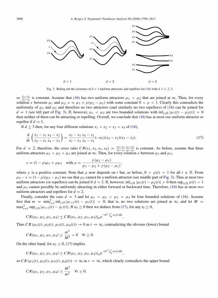
Fig. 3. Ruling out the existence of d + 1 uniform attractors and repellors for (16) with d = 1, 2, 3.

so x2−x1x3−x1

is constant. Assume that (16) has two uniform attractors µ1 < µ2 that are joined at ∞. Then, for everysolution x between µ1 and µ2, x = µ1 + ρ(µ2 − µ1) with some constant 0 < ρ < 1. Clearly this contradicts theuniformity of µ1 and µ2 and therefore no two attractors (and similarly no two repellors) of (16) can be joined ford = 1 (see left part of Fig. 3). If, however, µ1 < µ2 are two bounded solutions with inft∈R |µ1(t) − µ2(t)| > 0then neither of them can be attracting or repelling. Overall, we conclude that (16) has at most one uniform attractor orrepellor if d = 1.

If d ≤ 3 then, for any four different solutions x1 < x2 < x3 < x4 of (16),

ddt

(x3 − x1

x2 − x1

x4 − x2

x4 − x3

)=

x3 − x1

x2 − x1

x4 − x2

x4 − x3(−a3)(x4 − x1)(x3 − x2). (17)

For d = 2, therefore, the cross ratio C R(x1, x2, x3, x4) =x3−x1x2−x1

x4−x2x4−x3

is constant. As before, assume that threeuniform attractors µ1 < µ2 < µ3 are joined at ∞. Then, for every solution x between µ2 and µ3,

x = (1 − ρ)µ1 + ρµ3 with ρ =γ (µ2 − µ1)

µ3 − µ2 + γ (µ2 − µ1),

where γ is a positive constant. Note that ρ now depends on t but, as before, 0 < ρ(t) < 1 for all t ∈ R. Fromµ3 − x = (1 −ρ)(µ3 −µ1) we see that µ3 cannot be a uniform attractor (see middle part of Fig. 3). Thus at most twouniform attractors (or repellors) can be joined if d = 2. If, however, inft∈R |µ3(t)− µ2(t)| > 0 then supt∈R ρ(t) < 1and µ3 cannot possibly be uniformly attracting in either forward or backward time. Therefore, (16) has at most twouniform attractors and repellors for d = 2.

Finally, consider the case d = 3 and let µ1 < µ2 < µ3 < µ4 be four bounded solutions of (16). Assumefirst that m = min3

i=1 inft≥0 |µi+1(t) − µi (t)| > 0, that is, no two solutions are joined at ∞, and let M =

max3i=1 supt≥0 |µi+1(t)− µi (t)|. If a3 ≥ 0 then we deduce from (17), for any t0 ≥ 0,

C R(µ1, µ2, µ3, µ4) ≤ C R(µ1, µ2, µ3, µ4)|t0 e−m2 ∫ t

t0a3(s)ds

.

Thus C R (µ1(t), µ2(t), µ3(t), µ4(t)) → 0 as t → ∞, contradicting the obvious (lower) bound

C R(µ1, µ2, µ3, µ4) ≥m2

M2 > 0 ∀t ≥ 0.

On the other hand, for a3 ≤ 0, (17) implies

C R(µ1, µ2, µ3, µ4) ≥ C R(µ1, µ2, µ3, µ4)|t0 e−m2 ∫ t

t0a3(s)ds

,

so C R (µ1(t), µ2(t), µ3(t), µ4(t)) → ∞ as t → ∞, which clearly contradicts the upper bound

C R(µ1, µ2, µ3, µ4) ≤M2

m2 ∀t ≥ 0.


The only conceivable configuration containing four uniform attractors and repellors that is not covered by thepreceding argument and its “mirrored” version (i.e., considering t ≤ 0 instead of t ≥ 0) consists of a pair of attractors(µ1 < µ2, say) joined at ∞ and a pair of repellors (µ3 < µ4, say, with µ2 < µ3) joined at −∞ (see lower right partof Fig. 3; the configuration depicted in the upper right part of Fig. 3 for instance is ruled out by the above argumentfor t → −∞.). In this case, rewrite (17) in the form

ddt

C R(µ1, µ3, µ2, µ4) = C R(µ1, µ3, µ2, µ4)a3(µ4 − µ1)(µ3 − µ2),

to deduce that t 7→ C R(µ1, µ3, µ2, µ4) is monotone. For the configuration considered here, that is, for the caselimt→∞ (µ2(t)− µ1(t)) = limt→−∞ (µ4(t)− µ3(t)) = 0, we have

lim|t |→∞

C R(µ1, µ3, µ2, µ4) = 0.

Consequently C R(µ1, µ3, µ2, µ4) = 0, an obvious absurdity. With this it has been demonstrated that (17) cannothave four uniform attractors and repellors if d = 3. �

To the unprejudiced reader Theorem 21 must seem unsatisfactory, its statement being dictated solely by thelimitations of the simple arguments used in the course of the proof. It may thus come as a surprise that Theorem 21 isin a sense best possible, as will become apparent in the next section (Theorem 28 and Corollary 29).

3.3. Periodic differential equations

Apart from the asymptotically autonomous case, the simplest situation occurs in (3) if f is T -periodic in the firstargument, that is, if

f (t + T, x) = f (t, x), ∀(t, x) ∈ R2, (18)

with some T > 0. We shall see shortly that, as far as uniform attractors and repellors are concerned, even thisapparently tame class of equations allows for considerable structural complexity. First, however, we recall a fewsimple general facts about periodic differential equations. For the latter, the complete information about all solutionsof (3) is encoded in the family of local homeomorphisms Φs : x 7→ ϕ(s; 0, x), 0 ≤ s ≤ T , and in particular in ΦT ,the Poincare map associated with (3). More formally, for all (t0, x0) ∈ R2 and t ∈ R, and whenever ϕ(t; t0, x0) isdefined,

ϕ(t; t0, x0) = Φs2 ◦ ΦkT ◦ Φ−1

s1(x0),

where s1 = t0 − T bt0/T c, s2 = t − T bt/T c, and k = bt/T c − bt0/T c, hence 0 ≤ s1, s2 < T and k ∈ Z. Thereforethe long-term dynamics of (3) is governed by ΦT . For instance, µ is a pT -periodic solution with p ∈ N if and onlyif µ(0) is a fixed point of Φ p

T . Also, it is easy to see that the period of every non-constant periodic solution of (3) isa rational multiple of T , and in fact has to be of the form 1

q T for some q ∈ N (i.e., the solution is superharmonic)because ΦT is order-preserving [14,41].

Lemma 22. Let f satisfy (18) and assume that µ : R → R is a (forward, pullback, or uniform) attractor or a uniformrepellor of (3). Then µ is T -periodic.

Proof. Let µ be a bounded solution and observe that, since ΦT is monotone and µ(kT ) = ΦkT (µ(0)) for all k ∈ Z, the

sequence (µ(kT ))k∈Z is monotone and bounded. Hence the limits µ− = limk→−∞ µ(kT ) and µ+ = limk→∞ µ(kT )exist; moreover, ΦT (µ−) = µ− and ΦT (µ+) = µ+. Let ν−, ν+ denote the T -periodic solutions corresponding tothese two fixed points of ΦT , that is,

ν−(t) = ϕ(t; 0, µ−), ν+(t) = ϕ(t; 0, µ+) (t ∈ R).

From

|µ(t)− ν+(t)| =

∣∣∣∣Φt−T btT c

(µ

(T

⌊t

T

⌋))− Φt−T b

tT c(µ+)

∣∣∣∣ ≤ sup0≤s≤T

∣∣∣∣Φs

(µ

(T

⌊t

T

⌋))− Φs(µ+)

∣∣∣∣we see that |µ(t)− ν+(t)| → 0 as t → ∞. Analogously, |µ(t)− ν−(t)| → 0 as t → −∞.


Assume now that µ is a forward attractor. Since, for any δ > 0, |µ(t0) − ν−(t0)| < δ for some sufficiently smallt0, we find

0 = limτ→∞

|ϕ (t0 + τ ; t0, µ(t0))− ν−(t0 + τ)| = limt→∞

|µ(t)− ν−(t)|

and thus in particular |µ(kT )−ν−(kT )| = |µ(kT )−µ−| → 0 as k → ∞. Therefore µ+ = µ−, and µ is T -periodic.Next assume that µ is a pullback attractor. Given δ > 0, define x0,σ to be ν−(σ ) or µ(σ) depending on whether

|µ(σ)− ν−(σ )| < δ or not. Since, for all t ∈ R,

0 = limσ→−∞

|ϕ(t; σ, x0,σ )− µ(t)| = |ν−(t)− µ(t)|,

we find µ = ν−, hence µ is T -periodic.The remaining assertions are now obvious. �

As in the autonomous case, attractors of a T -periodic equation can be characterised easily in terms of the associatedPoincare map ΦT .

Theorem 23. Assume (18) holds, and let µ : R → R be a bounded solution of (3). Then the following statements areequivalent:

(i) µ is a forward attractor;(ii) µ is a pullback attractor;

(iii) µ is a uniform attractor;(iv) µ is T -periodic and µ(0) is an isolated fixed point of ΦT such that ΦT (a) − a > 0 > ΦT (b) − b for all

a < µ(0) < b with b − a sufficiently small.

Proof. Let µ be a forward or pullback attractor. By Lemma 22, µ is T -periodic and hence µ(0) is a fixed point of ΦT .If there existed a strictly increasing sequence (an)with an → µ(0) and ΦT (an) ≤ an for all n then Φk

T (an) 6→ µ(0) ask → ∞, so that µ could not be forward attracting. Setting x0,σ = an if σ/T is an integer, and x0,σ = µ(σ) otherwise,we would have

lim supk→−∞

|ϕ(0; kT, x0,kT )− µ(0)| ≥ |an − µ(0)| > 0

and thus µ would not be pullback attracting either. Overall, we see that (i) and (ii) both imply (iv).Conversely, assume that ΦT (a) − a > 0 > ΦT (b) − b for all a < µ(0) < b whenever b − a < ε. Pick δ > 0 so

small that⋃

0≤s≤T Φ−1s (]µ(s)− δ, µ(s)+ δ[) ⊂]µ(0)− ε, µ(0)+ ε[, i.e., whenever |x −µ(s)| < δ for some s with

0 ≤ s ≤ T then also |Φ−1s (x)− µ(0)| < ε. Assume now that supσ∈R |x0,σ − µ(σ)| < δ. Observing

|ϕ(σ + τ ; σ, x0,σ )− µ(σ + τ)| =

∣∣∣Φs2 ◦ ΦkT ◦ Φ−1

s1(x0,σ )− Φs2 (µ(0))

∣∣∣≤ sup

0≤s≤T

∣∣∣Φs ◦ ΦkT ◦ Φ−1

s1(x0,σ )− Φs (µ(0))

∣∣∣with s2 = σ + τ − T b(σ + τ)/T c, s1 = σ − T bσ/T c and k = b(σ + τ)/T c − bσ/T c, and noting that|Φ−1

s1(x0,σ ) − µ(0)| < ε for all σ ∈ R, we deduce that ‖ϕ(· + τ ; ·, x0,·) − µ(· + τ)‖∞ → 0 as τ → ∞. In

other words, µ is a uniform attractor. �

Corollary 24. Assume (18) holds, and let µ : R → R be a bounded solution of (3). Then µ is a uniform repellor ifand only if µ is T -periodic and µ(0) is an isolated fixed point of ΦT such that ΦT (a)− a < 0 < ΦT (b)− b for alla < µ(0) < b with b − a sufficiently small.

Remark 25. According to Lemma 22 and Theorem 23 an attractor µ cannot be subharmonic. It can, however, besuperharmonic, i.e., the minimal period of µ can be smaller than T and thus of the form 1

q T for some q ∈ N, q ≥ 2.For a simple example consider

x = 2 cos 2t + (1 + cos t) sin 2t − (1 + cos t)x,

for which f has minimal period 2π , yet the global uniform attractor µ : t 7→ sin 2t is π -periodic.


For T -periodic functions f it is natural to also study the averaged version of (3), i.e., the autonomous equation

x = f (x) where f (x) =1T

∫ T

0f (t, x)dt.

Note that f (x) is a polynomial whenever f (t, x) is polynomial in x . Sometimes information about solutions of (3) canbe obtained from the averaged equation, see for instance [39] for an introduction to the extensive theory of averaging.In the present context the averaging approach leads to

Theorem 26. Assume a0, a1, . . . , ad are continuous, T -periodic functions, and∫ T

0 ad(t)dt 6= 0. Then, for everysufficiently small ε > 0, the total number of uniform attractors and repellors of

x = ε(

a0(t)+ a1(t)x + · · · + ad(t)xd)

(19)

is at most d.

Proof. According to Theorem 21 the statement is true for d ≤ 2, even without any assumptions on ad and ε. We aretherefore interested only in the case d ≥ 3. For notational convenience we replace ε in (19) by εd−1. Thus modified,and rescaled via y = εx , (19) takes the form

y = ad yd+ εad−1 yd−1

+ · · · + εd−1a1 y + εda0. (20)

We are going to show that (20) has at most d uniform attractors and repellors, provided that ε > 0 is sufficiently small.Without loss of generality assume that

∫ T0 ad(t)dt > 0 as well as ad(0) > 0.

For ε = 0 the solution of (20) with y(0) = z is given by

y : t 7→z

(1 − (d − 1)Ad(t)zd−1)1

d−1

, (21)

where Ad(t) =∫ t

0 ad(s)ds, 0 ≤ t ≤ T . This solution exists for all 0 ≤ t ≤ T and z ∈ ]−C−

d ,C+

d [ where, if d is odd,

0 < C−

d = C+

d =

((d − 1) max

0≤t≤TAd(t)

)−1

(d−1)

< ∞,

whereas for even d the value of C+

d remains unchanged but

0 < C−

d =

(−(d − 1) min

0≤t≤TAd(t)

)−1

(d−1)

≤ ∞.

(If Ad(t) ≥ 0 for all t then C−

d is understood to equal ∞.) Correspondingly, the Poincare map associated with (20)can be written in the form

ΦT (z) =z

(1 − (d − 1)Ad(T )zd−1)1

d−1

+ εR(z, ε), (22)

where, for every compact set K ⊂] − C−

d ,C+

d [ and ε sufficiently small, R depends continuously on (z, ε) and is infact a (real-)analytic function of z. Moreover, uniformly on K ,

R(z, ε) → zd−1∫ T

0ad−1(t)

(1 − (d − 1)Ad(t)z

d−1) 1

d−1dt as ε → 0.

Similarly, integrating (20) in backward time, or inverting (22), yields

Φ−1T (z) =

z

(1 + (d − 1)Ad(T )zd−1)1

d−1

+ εS(z, ε),

a map analytic on ]−C−

d , C+

d [ where, as before, for odd d,

0 < C−

d = C+

d =

((d − 1)( max

0≤t≤TAd(t)− Ad(T ))

)−1

(d−1)

≤ ∞,


whereas for even d the number C+

d remains unchanged, yet

0 < C−

d =

((d − 1)(Ad(T )− min

0≤t≤TAd(t))

)−1

(d−1)

< ∞.

Note that, since Ad(T ) > 0, we have C+

d > C+

d ; also C−

d > C−

d or C−

d < C−

d depending on whether d is odd or even.It is easy to see that for every t0 ∈ [0, T ] with ad(t0) 6= 0 there exist positive numbers Dt0 , δt0 not depending on ε

such that, for any bounded solution ν of (20),

|ν(t)| ≤ Dt0 ∀t : |t − t0| < δt0 .

Assume now that νε is a T -periodic solution of (20). Since ad(0) > 0 we clearly have |νε(0)| ≤ D0 for all ε > 0. Asa key step in our analysis, we are going to show that actually

limε→0

νε(0) = 0. (23)

To this end, pick ν0 > C+

d and note that, according to (21), the solution of (20) with ε = 0 and y(0) = ν0becomes unbounded for some t∗ with 0 < t∗ ≤ T . By increasing ν0 slightly we may assume that ad(t∗) 6= 0.Pick δ < δt∗ so small that y(t∗ − δ) > Dt∗ . If, for some sequence (εn) with εn → 0, we had νεn (0) → ν0, that is, iflim supε→0 νε(0) ≥ ν0, then, by the continuous dependence on ε of the solutions of (20),

νεn (t∗

− δ) → y(t∗ − δ) > Dt∗ as n → ∞.

Clearly this would contradict the fact that, for all n,

|νεn (t)| ≤ Dt∗ ∀t : |t − t∗| < δt∗ .

Hence lim supε→0 νε(0) < ν0, and, since ν0 > C+

d was arbitrary, we deduce lim supε→0 νε(0) ≤ C+

d . Completelysimilar reasoning, using the fact that (21) becomes unbounded in forward (if d is odd) or backward time (if d is even)whenever y(0) < −C−

d , shows that lim infε→0 νε(0) ≥ −C−

d . To see that the inequalities in these relations are strictassume that νεn (0) → C+

d . Then

νεn (0) = Φ−1T

(νεn (0)

)→

C+

d

(1 + (d − 1)Ad(T )(C+

d )d−1)

1d−1

< C+

d ,

an obvious contradiction; for νεn (0) → −C−

d considering νεn (0) = Φ−1T

(νεn (0)

)if d is odd, and νεn (0) =

ΦT(νεn (0)

)if d is even, leads to a similar contradiction. We deduce from all this that

−C−

d < lim infε→0

νε(0) ≤ lim supε→0

νε(0) < C+

d .

Now the above argument can be iterated. Let νεn (0) → a and assume first that 0 ≤ a < C+

d . Then

a = limn→∞

νεn (0) = limn→∞

Φ−1T

(νεn (0)

)=

a

(1 + (d − 1)Ad(T )ad−1)1

d−1

,

and hence a = 0; similarly, if −C−

d < a ≤ 0 then a = 0. Thus we have established (23).

To conclude the proof, let ν(1)ε , . . . , ν(L)ε be L different uniform attractors or repellors of (20) and pick C <

min(C−

d ,C+

d ). Then |ν(i)ε (0)| < C for all i = 1, . . . , L and all sufficiently small ε. When considered a function of the

complex variable z, ΦT according to (22) is, for small ε, analytic on (an open set containing the closure of) the opendisc BC = {z : |z| < C} and, uniformly on BC ,

ΦT (z)− z →z

(1 − (d − 1)Ad(T )zd−1)1

d−1

− z =: G(z) as ε → 0.

The function G is analytic on Bmin(C−

d ,C+

d )and does not vanish on the boundary of BC . By Hurwitz’s Theorem (see

e.g. [37]) there exists ε0 > 0 such that, for all 0 < ε < ε0, the functions ΦT − idC and G have the same number of


zeros in BC , where all zeros are counted according to their multiplicity. Clearly, G(z) = 0 implies z = 0, and from

G(z) =z

(1 − (d − 1)Ad(T )zd−1)1

d−1

− z = Ad(T )zd

+O(z2d−1),

we see that z = 0 is a d-fold zero of G. Consequently, for ε < ε0, the Poincare map ΦT has exactly d complexfixed points; as a function of the real argument z, ΦT has at most d fixed points. Hence L ≤ d and the proof iscomplete. �

Remark 27. (i) The assumption∫ T

0 ad(t)dt 6= 0 in Theorem 26 ensures that the averaged right-hand side in (19) hasactual degree d . In this case, and if µε is a uniform attractor or repellor of (19) such that ε 7→ µε(0) is continuous,one can show that, uniformly in t ,

µε(t) → µ0 as ε → 0,

where µ0 is an equilibrium of the averaged equation, that is, p(µ0) = 0 with

p(x) =

∫ T

0a0(t)dt + x

∫ T

0a1(t)dt + · · · + xd

∫ T

0ad(t)dt.

An outline of the argument which extends [40, Thm. 3.1] is as follows: A lengthy yet elementary calculation yields arefined version of (22) for the representation of the Poincare map ΦT associated with (20), namely

ΦT (z) =z

(1 − (d − 1)Ad(T )zd−1)1

d−1

+

d∑i=1

εi Ri (z)+ εd+1 R(z, ε), (24)

where

Ri (z) = zd−i∫ T

0ad−i (t)dt +O(z2d−2i+1) (i = 1, . . . , d),

and, as before, the remainder term R(z, ε) is analytic in z and uniformly convergent as ε → 0. In terms of the originalcoordinate x , representation (24) has the form

ΦT (εx) = εx + εd p(x)+ εd+1 R(εx, ε).

If µε is a periodic solution of (19), again with ε replaced by εd−1, then

εµε(0) = ΦT (εµε(0)) = εµε(0)+ εd p (µε(0))+ εd+1 R(εµε(0), ε)

and hence, for all ε > 0,

p (µε(0))+ ε R(εµε(0), ε) = 0.

Since the proof of Theorem 26 has shown that εµε(0) → 0 as ε → 0, it follows that p (µε(0)) → 0 as well.Therefore, if ε 7→ µε is a continuous parametrisation then µε → µ0 with p(µ0) = 0.

(ii) An explicit (upper) bound for ε can be derived from an application of Rouche’s Theorem, see [35] for asomewhat similar result.

(iii) It is intriguing to speculate whether Theorems 23 and 26 might have any analogues for almost periodicequations. In general an attractor of (3) can be much more complicated if f = f (t, x) is merely almost periodicin t . However, it has been demonstrated in [41] that a form of uniformity (which, though different, does bear somesimilarity with the uniformity discussed here) greatly reduces the possible complexity of attractors.

We shall finally demonstrate that neither of the two assumptions in Theorem 26, namely smallness of ε andpreservation of the degree d under averaging, can be discarded easily. To see the importance of the smallness ofε, recall from Theorem 21 that the size of ε is irrelevant for the assertion in Theorem 26 as long as d ≤ 2, and also ifd = 3 and a3 does not change its sign. If, however, a3 does change its sign, then Theorem 26 generally fails for largerε, even if

∫ T0 a3(t)dt happens to be nonzero. This is the content of the following theorem which exploits an ingenious

idea in [30].


Theorem 28. Let a3 : R → R be continuous and T -periodic, and assume a3 does change its sign, i.e., a3(s)a3(t) < 0for some s, t ∈ R. Then, given N ∈ N, there exists a smooth, T -periodic function a2 such that

x = a2x2+ a3x3 (25)

has N uniform attractors.

Proof. We are going to construct a smooth, T -periodic function a such that

y = ay2+ ε2a3 y3 (26)

has N uniform attractors, provided that ε > 0 is sufficiently small. This will prove the theorem because settinga2 = a/ε and rescaling (26) via x = εy yields (25).

Given a3 with the stated properties it remains to find a such that, for small ε, (26) has N uniform attractors. To thisend, let A(t) =

∫ t0 a(s)ds and observe that the solution of (26) for ε = 0 and y(0) = z is given by

ϕ(t; 0, z) =z

1 − z A(t).

We will choose A 6= 0 such that A(0) = A(T ) = 0. Thus every solution of (26) for ε = 0 is T -periodic provided that|z| < (max0≤t≤T |A(t)|)−1

=: γ . The Poincare map associated with (26) can be written in the form

ΦT (z) = z + ε2 R(z)+ ε3S(z, ε), (27)

where R(z) = z3 Q A(z) and

Q A(z) =

∫ T

0

a3(t)

1 − z A(t)dt,

and S depends smoothly on z and ε. Assume that z0 6= 0 is a simple zero of R, i.e., R(z0) = 0 and R′(z0) 6= 0. Then,for every ε > 0 sufficiently small, there exists zε such that R(zε)+ εS(zε, ε) = 0 and hence ΦT (zε) = zε. Moreover,

Φ′

T (zε) = 1 + ε2 R′(zε)+ ε3 ∂

∂zS(zε, ε) 6= 1,

so that t 7→ ϕ(t; 0, zε) is, by Theorem 23, a uniform attractor or repellor of (26). Note that z0 is a zero of Q A also,and R′(z0) = z3

0 Q′

A(z0). The proof will therefore be complete once we can choose A in such a way that Q A hasN distinct zeros ζ1, . . . , ζN with Q′

A(ζi ) < 0 and 0 < ζi < γ for all i = 1, . . . , N . To this end, and denoting theindicator function of an arbitrary set M ⊂ R by 1M , we first use the (non-smooth) ansatz

A(t) =

2N∑i=1

αi 1Ii (t) (0 ≤ t ≤ T ), (28)

where the positive numbers αi and the compact intervals Ii ⊂]0, T [ will be chosen inductively below. In a final stepwe will afterwards approximate A from below by a C∞ function A, and a =

ddt A will have all the properties required.

Assume for the time being that∫ T

0 a3(t)dt > 0. Pick 2N different points 0 < t1, . . . , t2N < T such that

(−1)i a3(ti ) > 0 ∀i = 1, . . . , 2N . (29)

Define t0 = 0 and t2N+1 = T and let δ =12 min{|t j − tk | : j, k = 0, . . . , 2N + 1; j 6= k}; also define functions

Q(1), . . . , Q(2N ) as

Q(i)(z) =

∫ T

0a3(t)dt +

i∑j=1

α j z

1 − α j z

∫I j

a3(t)dt (i = 1, . . . , 2N ),

so that in particular Q(2N )= Q A with A according to (28). Set α1 = 1, and let I1 = [t1 −

12δ1, t1 +

12δ1]

with δ1 < δ so small that∫

I1a3(t)dt < 0. There exists a unique number ζ (1)1 with 0 < ζ

(1)1 < 1 such that

Q(1)(ζ(1)1 ) = 0 yet d

dz Q(1)(ζ(1)1 ) 6= 0 (see Fig. 4), i.e., ζ (1)1 is a simple root of Q(1). Next let α2 = 3/(ζ (1)1 + 2)


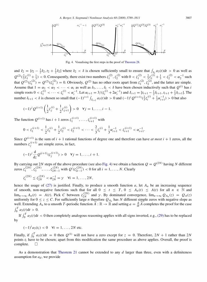
Fig. 4. Visualising the first steps in the proof of Theorem 28.

and I2 = [t2 −12δ2, t2 +

12δ2] where δ2 < δ is chosen sufficiently small to ensure that

∫I2

a3(t)dt > 0 as well as

Q(2)( 23ζ(1)1 +

13 ) < 0. Consequently, there exist two numbers ζ (2)1 , ζ

(2)2 with 0 < ζ

(2)1 < 2

3ζ(1)1 +

13 < ζ

(2)2 < α−1

2 such

that Q(2)(ζ(2)1 ) = Q(2)(ζ

(2)2 ) = 0. Obviously, Q(2) has no other roots apart from ζ

(2)1 , ζ

(2)2 , and the latter are simple.

Assume that 1 = α1 < α2 < · · · < αi as well as δ1, . . . , δi < δ have been chosen inductively such that Q(i) has isimple roots 0 < ζ

(i)1 < · · · < ζ

(i)i < α−1

i . Let αi+1 = 3/(ζ (i)i + 2α−1i ) and Ii+1 = [ti+1 −

12δi+1, ti+1 +

12δi+1]. The

number δi+1 < δ is chosen so small that (−1)i+1∫

Ii+1a3(t)dt > 0 and (−1)i Q(i+1)( 2

3ζ(i)i +

13α

−1i+1) > 0 but also

(−1) j Q(i+1)(

12ζ(i)j +

12ζ(i)j+1

)> 0 ∀ j = 1, . . . , i − 1.

The function Q(i+1) has i + 1 zeros ζ (i+1)1 , . . . , ζ

(i+1)i+1 with

0 < ζ(i+1)1 <

12ζ(i)1 +

12ζ(i)2 < ζ

(i+1)2 < · · · <

23ζ(i)i +

13α−1

i+1 < ζ(i+1)i+1 < α−1

i+1.

Since Q(i+1) is the sum of i + 1 rational functions of degree one and therefore can have at most i + 1 zeros, all thenumbers ζ (i+1)

j are simple zeros, in fact,

(−1) j ddz

Q(i+1)(ζ(i+1)j ) > 0 ∀ j = 1, . . . , i + 1.

By carrying out 2N steps of the above procedure (see also Fig. 4) we obtain a function Q = Q(2N ) having N differentzeros ζ (2N )

1 , ζ(2N )3 , . . . , ζ

(2N )2N−1 with Q′(ζ

(2N )2i−1 ) < 0 for all i = 1, . . . , N . Clearly

ζ(2N )i ≤ ζ

(2N )2N < α−1

2N = γ ∀i = 1, . . . , 2N ,

hence the usage of (27) is justified. Finally, to produce a smooth function a, let An be an increasing sequenceof smooth, non-negative functions such that for all 0 ≤ t ≤ T , 0 ≤ An(t) ≤ A(t) for all n ∈ N andlimn→∞ An(t) = A(t). Pick C between ζ (2N )

2N and γ . By dominated convergence, limn→∞ Q An (z) = Q A(z)uniformly for 0 ≤ z ≤ C . For sufficiently large n therefore Q An has N different simple zeros with negative slope aswell. Extending An to a smooth T -periodic function A : R → R and setting a =

ddt A completes the proof for the case∫ T

0 a3(t)dt > 0.

If∫ T

0 a3(t)dt < 0 then completely analogous reasoning applies with all signs inverted, e.g., (29) has to be replacedby

(−1)i a3(ti ) < 0 ∀i = 1, . . . , 2N etc.

Finally, if∫ T

0 a3(t)dt = 0 then Q(1) will not have a zero except for z = 0. Therefore, 2N + 1 rather than 2Npoints ti have to be chosen; apart from this modification the same procedure as above applies. Overall, the proof iscomplete. �

As a demonstration that Theorem 21 cannot be extended to any d larger than three, even with a definitenessassumption for ad , we provide


Corollary 29. Let d ≥ 4 be a natural number, and assume ad : R → R is continuous, T -periodic and either non-negative or non-positive. Then, given N ∈ N, there exist smooth, T -periodic functions a2, a3 such that

x = a2x2+ a3x3

+ ad xd (30)


Proof. Up to and including terms of order ε2, the Poincare map ΦT associated with

y = ay2+ ε2a3 y3

+ εd−1ad yd (31)

is identical with the one in the previous proof, that is, (27) holds with only the remainder term S modified. Thus,taking as a3 any smooth, T -periodic function which changes its sign and subsequently constructing a as in the proofof Theorem 28, we conclude that (31) has N uniform attractors whenever ε > 0 is sufficiently small. Setting a2 = a/εand rescaling (31) via x = εy yields (30). �

Our final result highlights the role of the non-degeneracy condition∫ T

0 ad(t)dt 6= 0 in Theorem 26 by showing thatthe latter generally fails if this condition is not met.

Corollary 30. Let d ≥ 3 be a natural number and ad 6= 0 a continuous, T -periodic function with∫ T

0 ad(t)dt = 0.Then, given N ∈ N, there exists a smooth T -periodic function a2 such that, for all sufficiently small ε > 0,

x = ε(a2x2+ adxd) (32)


Proof. The argument is quite similar to the one proving Theorem 28. Clearly, the assertion remains unchanged if, fornotational convenience, ε is replaced by εd−1 in (32). Thus modified, and rescaled via x = y/ε, (32) takes the form

y = εd−2a2 y2+ ad yd . (33)

The proof will therefore be complete once we demonstrate how to find a2 not depending on ε such that (33) has Nuniform attractors or repellors for all sufficiently small ε > 0.

Let Ad =∫ t

0 ad(s)ds and note that Ad(0) = Ad(T ) = 0. Similarly to (27) the Poincare map ΦT associated with(33) can be written as

ΦT (z) = z + εd−2 R(z)+ εd−1S(z, ε) (34)

with R(z) = z2 Qa2(z) and

Qa2(z) =

∫ T

0a2(t)

(1 − (d − 1)Ad(t)z

d−1) d−2

d−1dt,

provided that |z| < Cd , where

Cd =

((d − 1) max

0≤t≤T|Ad(t)|

)−1

d−1

> 0.

As before, it only remains to choose a2 in such a way that Qa2 has N simple zeros within the interval ]0,Cd [.Obviously, Qa2 depends linearly upon a2, and, for |z| < Cd ,

Qa2(z) =

∞∑k=0

d − 2d − 1

k

(1 − d)k zk(d−1)∫ T

0a2(t)A

kd(t)dt.

Thus, if a2 is orthogonal to 1 (=A0d), Ad , . . . , Ai−1

d yet not orthogonal to Aid then the leading term of Qa2(z) will be

of the order zi(d−1). More formally, choose N smooth, T -periodic functions a(i)2 , i = 1, . . . , N such that, for all i ,∫ T

0a(i)2 (t)dt =

∫ T

0a(i)2 (t)Ad(t)dt = · · · =

∫ T

0a(i)2 (t)Ai−1

d (t)dt = 0 yet∫ T

0a(i)2 (t)Ai

d(t)dt 6= 0.


(Such a choice is possible because Ad is continuous but not constant.). With this,

Qa(i)2(z) = qi z

i(d−1)+O(z(i+1)(d−1)) (i = 1, . . . , N ),

with constants qi 6= 0. From (a slightly generalised version of) [30, Lem. 3.1] it follows that there exist positivenumbers γ1, . . . , γN such that with

a2 = γN a(N )2 − γN−1a(N−1)2 + · · · + (−1)N−1γ1a(1)2

the function Qa2 has N simple zeros in ]0,Cd [. �

4. Concluding remarks

The success of classical bifurcation theory for autonomous differential equations x = F(x; λ) which depend on aparameter λ is due to several facts which, albeit obvious, have to be reconsidered carefully when a nonautonomousbifurcation theory is to be developed:

(i) Many relevant models in applied sciences are indeed of the form x = F(x; λ);(ii) Potential bifurcating objects like equilibria and periodic orbits are characterised algebraically as zeros of F and

a Poincare map, respectively;(iii) Usually, there are not too many bifurcating objects, and the generic ones can to some extent be classified [2];(iv) Asymptotic stability of equilibria and periodic orbits can be determined through linear algebra by means of,

respectively, the linearisation of F and a Poincare map;(v) The transient behaviour of solutions is related to their asymptotic behaviour; more precisely, the long-term

dynamics of an attractive equilibrium or periodic orbit can be approximated arbitrarily well by the transientbehaviour on longer and longer time intervals. In particular, finite time numerics can be used to approximateasymptotic behaviour.

The results in this article show that in many respects the nonautonomous situation remains fundamentally differentfrom the autonomous one, and the simple facts provided here allow for a clear understanding as to why this is so.Concretely, when reconsidering the above list in an nonautonomous setting one is lead naturally to a variety offundamental questions which we feel are largely open at present.

(i)t What are the characteristics of a prototypical nonautonomous model x = f (t, x; λ)? How can one choose theappropriate time dependence for f ? So far, we have studied nonautonomous attraction and repulsion only inits simplest uniform version for scalar equations. Already an astonishing dynamical complexity emerges whichis in a sense due to the lack of better knowledge about how precisely f depends on t or, more positively put,the amazing “degree of freedom” which comes with time-varying vector fields. For example, our analysis ofperiodic equations does not incorporate the rate ∂

∂t f at which f is changing in time. On the other hand, this rateis known to play a prominent role for instance in explicit conditions ensuring asymptotic stability (albeit in aslightly different context, see [11]). We feel it necessary to push for the development, driven by applications, ofa methodology of nonautonomous modelling.

(ii)t Uniformly attracting or repelling solutions cannot be detected algebraically, e.g. by looking for zeros off . Rather, the asymptotic behaviour and the spatial structure of (1)t tend to be interwoven in an intricatemanner. Theorems 17 and 26 may serve as simple but perhaps prototypical examples. In fact, we expect thatmost questions regarding uniform attractors will touch upon a delicate balance between temporal and spatialcomplexity (see also [28]). Versatile, effective tools for analysing this balance have yet to be developed.

(iii)t In view of Theorems 26 and 28 it appears doubtful whether the clear-cut situation for autonomous equations(i.e., few, classifiable bifurcation scenarios) does have an analogue in the nonautonomous setting. If so,a satisfactory treatment of the classification problem is desirable; if not, a bewildering zoo of bifurcationphenomena is likely to await exploration.

(iv)t Attraction or repulsion of a solution can in general not be determined directly from the coefficients of thelinearisation (see e.g. the instructive example in [28]). To comprehensively cover uniform attractors and repellorsthe existing asymptotic methods for nonautonomous equations will need substantial refinement.


(v)t What is the transient behaviour of a uniformly attracting or repelling solution, in particular, how repelling can auniformly attracting solution be on an arbitrary bounded interval in time? We argue that this question is relevantnot only for obvious practical reasons (as for instance no physical observation can cover an infinite intervalin time) but also for mathematical reasons. In view of the enormous freedom introduced via an explicit yetunspecified time dependence in (1)t it is plausible that quite generally asymptotic concepts are of limited useand finite time concepts may step in.

In the context of (v)t we mention in closing a recent approach [5,12] that avoids any assumptions on the timedependence of f and that instead studies the transient behaviour of (1)t on intervals of finite time by exploitingall available (numerical) information. A solution x of (1)t on a finite time interval [a, b] is attracting if S(t) :=∂∂x f (t, x(t)), or more generally the symmetric matrix S(t) :=

12

[∂∂x f (t, x(t))+

∂∂x f (t, x(t))T

]if x ∈ Rn , n ≥ 2,

is negative (definite) for all t ∈ [a, b]. As a consequence, if x is attracting then all solutions which are close to xhave a decreasing distance from x on [a, b]; analogously, x is repelling if S(t) is positive (definite) for all t ∈ [a, b].It is easy to see that the polynomial equation (16) with arbitrary time dependence on [a, b] has at most d connectedcomponents in [a, b]×R such that each component consists entirely of attracting or repelling solutions. Observationslike these suggest that finite time concepts may indeed complement asymptotic concepts and may thus contributetowards a better understanding of nonautonomous differential equations.

Acknowledgements

The first author was partially supported by a HUMBOLDT Research Fellowship; he wishes to express his gratitudeto the Johann Wolfgang Goethe-Universitat Frankfurt for the hospitality he enjoyed during his visits in 2005 and 2006.The second author was supported by the EMMY NOETHER Program funded by the Deutsche Forschungsgemeinschaft.

References

[1] M.A.M. Alwash, Periodic solutions of polynomial non-autonomous differential equations, Electron. J. Differential Equations 84 (2005) 1–8.[2] V.I. Arnold, Dynamical Systems V. Bifurcation Theory and Catastrophe Theory, in: Encyclopedia of Mathematical Sciences, vol. V, Springer,

Berlin, Heidelberg, New York, 1994.[3] B. Aulbach, T. Wanner, Integral manifolds for Caratheodory type differential equations in Banach spaces, in: B. Aulbach, F. Colonius (Eds.),

Six Lectures on Dynamical Systems, World Scientific, Singapore, 1996.[4] B. Aulbach, T. Wanner, The Hartman–Grobman theorem for Caratheodory-type differential equations in Banach spaces, Nonlinear Anal.

TMA 40 (2000) 91–104.[5] A. Berger, T.S. Doan, S. Siegmund, Nonautonomous finite-time dynamics, 2007. Preprint.[6] D.N. Cheban, P.E. Kloeden, B. Schmalfuss, The relationship between pullback, forward and global attractors of nonautonomous dynamical

systems, Nonlinear Dyn. Syst. 2 (2002) 125–144.[7] H. Crauel, A. Debusche, F. Flandoli, Random attractors, J. Dynam. Differential Equations 9 (1997) 307–341.[8] H. Crauel, F. Flandoli, Attractors for random dynamical systems, Probab. Theory Related Fields 100 (1994) 365–393.[9] H. Crauel, P. Imkeller, M. Steinkamp, Bifurcations of one-dimensional differential equations, in: H. Crauel, V.M. Gundlach (Eds.), Stochastic

Dynamics, Springer, 1999, pp. 27–47.[10] J. Devlin, Periodic solutions of polynomial non-autonomous differential equations, Proc. Soc. Roy. Edinburgh Sect. A 123 (1993) 783–801.[11] L.H. Duc, A. Ilchmann, S. Siegmund, P. Taraba, On stability of linear time-varying second-order differential equations, Quart. Appl. Math.

64 (2006) 137–151.[12] L.H. Duc, S. Siegmund, Hyperbolicity and invariant manifolds for planar nonautonomous systems on finite time intervals, 2006. Preprint.[13] R. Fabbri, R.A. Johnson, F. Mantellini, A nonautonomous saddle-node bifurcation pattern, Stoch. Dyn. 4 (2004) 335–350.[14] J. Hale, H. Kocak, Dynamics and Bifurcations, Springer, New York, 1991.[15] M.C. Irwin, Smooth Dynamical Systems, Academic Press, New York, London, 1980.[16] R.A. Johnson, An application of topological dynamics to bifurcation theory, in: M.G. Nerurkar, D.P. Dokken, D.B. Ellis (Eds.), Topological

Dynamics and Applications. A Volume in Honor of Robert Ellis, in: Contemporary Mathematics, vol. 215, American Mathematical Society,Providence, Rhode Island, 1998, pp. 323–334.

[17] R.A. Johnson, P.E. Kloeden, R. Pavani, Two-step transition in nonautonomous bifurcations: An explanation, Stoch. Dyn. 2 (2002) 67–92.[18] R.A. Johnson, F. Mantellini, A nonautonomous transcritical bifurcation problem with an application to quasi-periodic bubbles, Discrete

Contin. Dyn. Syst. 9 (2003) 209–224.[19] R.A Johnson, Y. Yi, Hopf bifurcation from non-periodic solutions of differential equations, II, J. Differential Equations 107 (1994) 310–340.[20] O.G. Khudaıberenov, N.O. Khudaıverenov, An estimate for the number of periodic solutions of the Abel equation, Differ. Uravn. 8 (2004)

1140–1142.[21] P.E. Kloeden, Pullback attractors in nonautonomous difference equations, J. Differ. Equations Appl. 6 (2000) 33–52.[22] P.E. Kloeden, Pitchfork and transcritical bifurcations in systems with homogeneous nonlinearities and an almost periodic time coefficient,

Commun. Pure Appl. Anal. 3 (2004) 161–173.


[23] P.E. Kloeden, H. Keller, B. Schmalfuß, Towards a theory of random numerical dynamics, in: H. Crauel, V.M. Gundlach (Eds.), StochasticDynamics, Springer, 1999, pp. 259–282.

[24] P.E. Kloeden, B. Schmalfuß, Nonautonomous systems, cocycle attractors and variable time-step discretization, Numer. Algorithms 14 (1997)141–152.

[25] P.E. Kloeden, S. Siegmund, Bifurcations and continuous transitions of attractors in autonomous and nonautonomous systems, Internat. J.Bifur. Chaos Appl. Sci. Engrg. 5 (2005) 1–21.

[26] J.A. Langa, J.C. Robinson, A. Rodriguez-Bernal, A. Suarez, A. Vidal-Lopez, Existence and nonexistence of unbounded forwards attractor fora class of nonautonomous reaction diffusion equations, Discrete Contin. Dyn. Syst. 18 (2007) 483–497.

[27] J.A. Langa, J.C. Robinson, A. Suarez, Stability, instability, and bifurcation phenomena in non-autonomous differential equations, Nonlinearity15 (2002) 887–903.

[28] J.A. Langa, J.C. Robinson, A. Suarez, Bifurcations in non-autonomous scalar equations, J. Differential Equations 221 (2006) 1–35.[29] D. Li, P.E. Kloeden, Equi-attraction and the continuous dependence of pullback attractors on parameters, Stoch. Dyn. 4 (2004) 373–384.[30] A. Lins Neto, On the number of solutions of the equation dx

dt =∑n

j=0 a j (t)xj , 0 ≤ t ≤ 1, for which x(0) = x(1), Invent. Math. 59 (1980)

67–76.[31] N.G. Lloyd, The number of periodic solutions of the equation z = zN

+ p1(t)zN−1

+ · · · + pN (t), Proc. London Math. Soc. 27 (1973)667–700.

[32] I. Malta, N.C. Saldanha, C. Tomei, Morin singularities and global geometry in a class of ordinary differential operators, Topol. MethodsNonlinear Anal. 10 (1997) 137–169.

[33] L. Markus, Asymptotically autonomous differential systems, Annal. Math. Studies 3 (1956) 17–29.[34] K.J. Palmer, A generalization of Hartman’s linearization theorem, J. Math. Anal. Appl. 41 (1973) 753–758.[35] A.A. Panov, The number of periodic solutions of polynomial differential equations, Math. Notes 64 (1998) 622–628.[36] M. Rasmussen, Attractivity and Bifurcations for Nonautonomous Dynamical Systems, in: Lecture Notes in Mathematics, vol. 1907, Springer,

New York, 2007.[37] R. Remmert, Theory of Complex Functions, Springer, New York, 1991.[38] R.J. Sacker, G.R. Sell, A spectral theory for linear differential systems, J. Differential Equations 27 (1978) 320–358.[39] J.A. Sanders, F. Verhulst, Averaging Methods in Nonlinear Dynamical Systems, Springer, New York, 1985.[40] S. Shashahani, Periodic solutions of polynomial first order differential equations, Nonlinear Anal. TMA 5 (1981) 157–165.[41] W. Shen, Y. Yi, Almost automorphic and almost periodic dynamics in skew-product semiflows, Mem. Amer. Math. Soc. 136 (647) (1998).[42] S. Siegmund, Dichotomy spectrum for nonautonomous differential Equations, J. Dynam. Differential Equations 14 (2002) 243–258.[43] A.N. Sositaisvili, Bifurcations of topological type at singular points of parametrized vector fields, Funct. Anal. Appl. 6 (1972) 169–170.

Translation from Funkts. Anal. Prilozh. 6 97–98.[44] H.R. Thieme, Convergence results and a Poincare–Bendixson trichotomy for asymptotically autonomous differential equations, J. Math. Biol.

30 (1992) 755–763.[45] H.R. Thieme, Asymptotically autonomous differential equations in the plane, Rocky Mountain J. Math. 24 (1994) 351–380.[46] P.J. Torres, Existence of closed solutions for a polynomial first order differential equation, J. Math. Anal. Appl. 328 (2007) 1108–1116.[47] W. Walter, Ordinary Differential Equations, Springer, New York, 1998.[48] Y. Yi, A generalized integral manifold theorem, J. Differential Equations 102 (1993) 153–187.

uniformly attracting solutions of nonautonomous ...aberger/papers/uniform... · uniformly...

Documents