unified theory of credit spreads and defaults - northfield · unified theory of credit spreads and...

Unified Theory of Credit Spreads and

Defaults

Emilian Belev and Dan diBartolomeo Newport, RI June 3, 2016

www.northinfo.com

School 1: Theory of Bonds and Credit Spreads

Slide 2

www.northinfo.com

School 2: Theory of Contingent Claims Credit

Slide 3

-10

-5

0

5

10

15

Corporate Asset Distribution

Corporate Debt

Asset Level

Inputs to Credit Model: σ Debt Asset Level Model States: βbond = βstock * -(Pstock / Pbond) * (Δput/ Δcall) Corollaries: ① LGD = Pbond* scalar; ② LGD & OAS Prob. Default

Asset Return

Probability Density

www.northinfo.com

What is the Credit Spread to MVO Investor

Slide 4

0

0.01

0.02

0.03

0.04

0.05

0.06

0.07

0.08

0 0.05 0.1 0.15 0.2 0.25 0.3

Efficient Frontier

Tangent

Investor Utility

www.northinfo.com

OAS as an Intercept and Link to Risk Premium

Slide 5

0

0.01

0.02

0.03

0.04

0.05

0.06

0.07

0.08

0 0.05 0.1 0.15 0.2 0.25 0.3

Spread

Risk Premium

www.northinfo.com

An Apparent Paradox

• Assuming constant treasury rates, we can view OAS is the “Certainty Equivalent” from utility theory: “If I was offered an investment with no credit risk, or this risky investment, what is the deterministic rate of return that is going to make me indifferent ?”

• Then by exponential expected utility: OAS = Expected Return – Aversion Coefficient * Variance • Paradox: for an risk-averse investor it appears that OAS < Expected Return

• But in practice OAS is always > Expected Return

• To resolve this we will start with a numerical example of two bonds – “investment grade”

bond and a “junk” bond.

Slide 6

www.northinfo.com

A Tale of Two Bonds

• An “investment grade” bond offering these payoffs (and probabilities): • $100 (75%) • $90 (20%) • $20 (5%)

• A “junk” bond offering these payoffs and probabilities:

• $100 (10%) • $30 (50%) • $20 (40%)

• For both cases, at any entry price, the OAS will be higher than the expected return because

the OAS will produce $100 for all outcomes.

Slide 7

www.northinfo.com

A Tale of Two Bonds (cont’d)

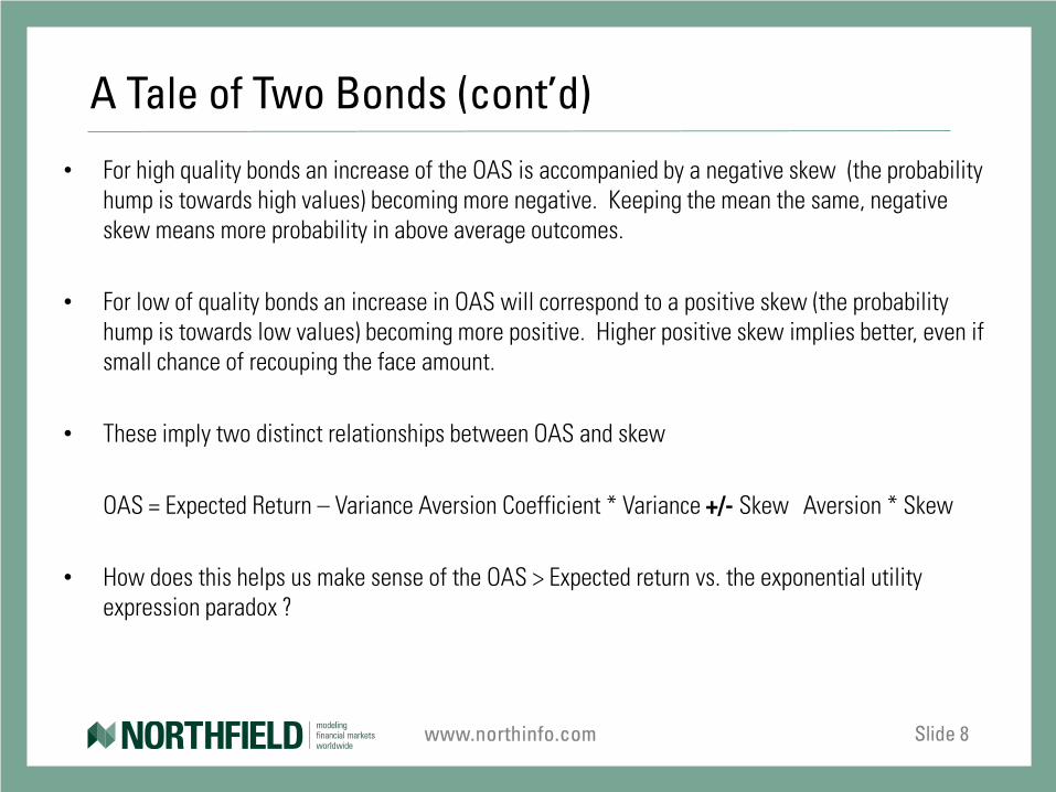
• For high quality bonds an increase of the OAS is accompanied by a negative skew (the probability hump is towards high values) becoming more negative. Keeping the mean the same, negative skew means more probability in above average outcomes.

• For low of quality bonds an increase in OAS will correspond to a positive skew (the probability

hump is towards low values) becoming more positive. Higher positive skew implies better, even if small chance of recouping the face amount.

• These imply two distinct relationships between OAS and skew OAS = Expected Return – Variance Aversion Coefficient * Variance +/- Skew Aversion * Skew • How does this helps us make sense of the OAS > Expected return vs. the exponential utility

expression paradox ?

Slide 8

www.northinfo.com

A Small Detour: Entropy

Slide 9

www.northinfo.com

Maximum Entropy Principle

Slide 10

Probability Density -6

-4

-2

0

2

4

6

0 0.1 0.2 0.3 0.4 0.5 0.6 0.7 0.8

Normal

Montary Response

Higher Entropy Lower Entropy

In the absence of additional information the most conservative assumption is to assume all probabilities are the same – uniform distribution is the limiting case.

www.northinfo.com

Implications of Maximum Entropy Principle

• Assume investors are aware of distributional higher moments of the distribution but they cannot reliably estimate them • By definition higher moment events occur in the tails and thus too rarely to be reliably

estimated

• Based on the Maximum Entropy Principle, however, in utility terms, investors can consider the combined impact of variance with higher moments for truncated distributions like that of a bond.

• For bonds with positive skew (low credit quality) the principle will entail that in the absence of any other information an increase in variance will increase the positive skew

• For bonds with negative skew (high credit quality), in the absence of any other information an increase in variance will decrease in the negative skew Slide 11

www.northinfo.com

Variance Increase: Positive Skew Impact

Slide 12

Credit Distribution

Expected Value

www.northinfo.com

Variance Increase: Negative Skew Impact

Slide 13

Credit Return Distribution

Expected Value

www.northinfo.com

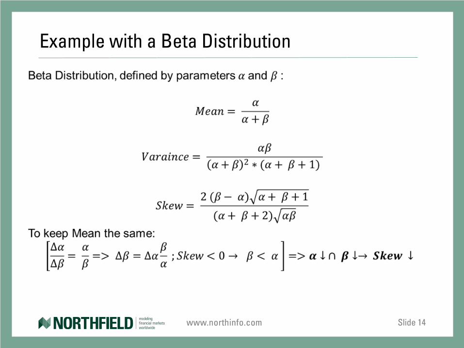
Example with a Beta Distribution

Slide 14

www.northinfo.com

Summary of Utility Equality

• “Investment Grade” Bonds: investors like outcomes close to principal protection, which entails negative skew acceptance parameter:

OAS = Expec ted Return – Variance Aversion Coeffic ient * Variance - Skew Coeffic ient * (negative Sk ew)

By entropy, as variance increases Skew becomes more negative, which may overcompensate for positive

variance aversion in terms of preference • “Junk” Bonds: investors like speculative outcomes close to unlikely return of principal, which entails

positive skew acceptance parameter:

OAS = Expec ted Return – Variance Aversion Coeffic ient * Variance + Skew Coeffic ient * (positive) Sk ew

We then can approximate via: OAS = Expected Return + Adjusted Aversion Coefficient * Variance

Slide 15

www.northinfo.com

Higher Moments of Log Return

Slide 16

www.northinfo.com

Higher Moments of Log Return (cont’d)

Slide 17

www.northinfo.com

Incorporating Higher Moments in MVO

• As shown previously, we project the truncated distribution of credit payoff – the segment under the debt level

• Then we can calculate higher moments and based on the leverage-based utility function (adjusted or

unadjusted) we can estimate the equivalent increase in variance that will reflect the higher moments plus the aversion to them

• We ca also approach the incorporation of higher moments indirectly

Slide 18

-10

-5

0

5

10

15 Corporate Asset Distribution

Corporate Debt

Asset Level

www.northinfo.com

Back to the Spread as a Certainty Equivalent

OAS = Expected Return + Adjusted Aversion Coefficient * Variance Can be represented as: OAS = E[Return Credit] + E[Other Factor] + Adjusted Aversion Coefficient *

[Variance(Credit) + Variance(Other Factor)] • “Other Factor” can be e.g. liquidity. • If we want to capture the “Other Factor” for a group of bonds we can run a cross sectional

regression of OAS per bucket against “Merton”-style volatilities of the constituents. • Cont’d

Slide 19

www.northinfo.com

Back to Spread as Certainty Equivalent (cont’d)

• We would expect from the slope of that regression to be positive based on previous arguments

• We would expect the intercept of that regression to consist of the average expected returns of the group of bonds plus the volatility aversion term to the “Other Factor.”

• We would expect the residuals of that regression to consist of divergences in expected return and errors due to higher moment effects.

• In the absence of “Other Factor”, if the credit distributions for all bonds in the bucket are stationary, then the regression intercept (the average spread) and slope will be identical through time.

• If the expectation and/or variance of “Other Factor” changes over time, then the intercept OAS will change.

Slide 20

www.northinfo.com

The Importance of the Intercept

OAS = E[Return Credit] + E[Other Factor] + Adjusted Aversion Coefficient * [Variance(Credit) + Variance(Other Factor)]

• If we pick a bucket by a particular credit band (e.g. BB) and accept that E[Return Credit] and the

variance terms are constant over time, the change of period to period of the intercept will be due to the changes in E[Other Factor]

• The volatility of this spread will be related to additional volatility of the bonds in that bucket beyond Merton-style volatility through the spread duration of the particular bond. We can use times series of this variable as the basis for (an) additional risk factor(s)

• Also the volatility of that component for the bucket can be found by using the average spread duration of the bucket. Having found this quantity we can subtract from the intercept to find the contemporaneous expected return. This is an important step in an alternate way to estimate higher moments of bond distribution.

Slide 21

www.northinfo.com

Higher Moments 2

• Having estimated E[R] and VAR we can build a lattice of credit quality transition, trace the paths

and estimate higher moments of the full resulting distribution.

• The benefit of this method is that assumes piece wise distribution but lets the full distribution of credit quality naturally arise rather than use a parameterized one. Also, this approach mitigates the “limited observation” aspect of higher moment estimation.

Slide 22

AAA AAA

AA

AAA

A

AAA

AA

BBB

www.northinfo.com

Higher Moments Yet Again

OAS = E[Return Credit] + E[Other Factor] + Adjusted Aversion Coefficient * [Variance(Credit) + Variance(Other Factor)] • What if the E[R] and VAR are changing over time. Or what if Aversion is not constant over time.

• Isaac Newton vs. Christiaan Huygens argued about light being a wave or a particle. Eventually we

settled that it is both.

• Didier Sornette and Nassim Taleb have argued about Dragon Kings vs. Black Swans – i.e. economic distributions are subject to changing regimes vs. they are subject to truly unknown higher moments. May be we should settle that these two views are two sides of the same phenomenon that plays out over time.

• If we keep our “intercept” factor observations relatively short we would be able to capture the changing

nature of mean and variance and adapt the model to higher moments.

Slide 23

www.northinfo.com

Empirical Results with Spreads and Volatilities

The data set consisted of credit spreads for 5 years (EOY) and their contemporaneous Merton-style volatilities. That entails 5 sets of approx. 200K bonds each with OAS calculated by Northfield per period.

The fundamental purpose of this analysis was to observe the cross-sectional relationship

between spreads and Merton-style volatilities, and its evolution over time. The variables to which we would pay special are: - Positive or negative correlation (sign of the slope) - Statistical significance of slope - Statistical significance of intercept - Relative size of the intercept across buckets - Relative size of the intercept cross buckets

Slide 24

www.northinfo.com

All Bonds Snapshot 2015-12-31

Slide 25

0

0.2

0.4

0.6

0.8

1

0 0.01 0.02 0.03 0.04 0.05 0.06 0.07 0.08 0.09 0.1

All data points Dec-31 2015

Liner Fit

Coefficients t Stat Intercept 0.049 33.965 X Variable 1 3.333 15.262

0

1000

2000

3000

4000

0 500 1000 1500 2000 2500 3000 3500 4000

Rank Merton Varaince vs. OAS

Linear Fit

Spearman Correlation: 0.412

www.northinfo.com

A Sample Plot for a Bucket: “A”-rated

VAL T-STAT

SLOPE 6.295828 12.20471

INTERCEPT 0.010829 33.35786

Slide 26

0

0.02

0.04

0.06

0.08

0.1

0.12

0.14

0 0.001 0.002 0.003 0.004 0.005 0.006 0.007 0.008

www.northinfo.com

A Sample Plot for a Bucket: “B”-rated

Slide 27

VAL T-STAT

SLOPE 12.46111 9.256393

INTERCEPT 0.066457 8.593081

0

0.1

0.2

0.3

0.4

0.5

0.6

0.7

0.8

0 0.005 0.01 0.015 0.02 0.025

BofA ML US B spread: 7.15%

www.northinfo.com

A Sample Plot for a Bucket: “CCC”-rated

VAL T-STAT

SLOPE 8.593996 4.066664

INTERCEPT 0.156904 6.384991

Slide 28

0

0.1

0.2

0.3

0.4

0.5

0.6

0.7

0.8

0.9

1

0 0.005 0.01 0.015 0.02 0.025 0.03 0.035 0.04 0.045 0.05

BofA ML US CCC spread: 16. 53 %

www.northinfo.com

Summary Results for 2015-12-31

Slide 29

Year Credit Band Coefficient Value T-statistic

2015

AAA SLOPE 1.408 2.391

INTERCEPT 0.007 12.003

AA SLOPE 0.241 2.831


A SLOPE 6.296 12.205


BBB SLOPE 10.673 15.056


BB SLOPE 6.712 7.709


B SLOPE 12.461 9.256


CCC SLOPE 8.594 4.067


www.northinfo.com


Slide 30


2014

AAA SLOPE 0.197 3.727


AA SLOPE 0.359 12.132


A SLOPE 0.452 10.400


BBB SLOPE 0.197 1.539


BB SLOPE 0.172 0.863


B SLOPE 0.121 1.323


www.northinfo.com


Slide 31


2013

AAA SLOPE 0.200 2.858


AA SLOPE 0.305 10.826


A SLOPE -0.021 -0.496


BBB SLOPE 0.190 2.305


BB SLOPE 1.147 6.449


B SLOPE 0.163 0.158


www.northinfo.com


Slide 32


2012

AAA SLOPE 0.155 7.836


AA SLOPE 0.317 15.393


A SLOPE 0.263 6.500


BBB SLOPE 0.404 5.691


BB SLOPE 0.968 5.562


B SLOPE 0.466 0.259


www.northinfo.com


Slide 33


2011

AAA SLOPE -1.321 -3.093


AA SLOPE 15.434 4.684


A SLOPE 2.704 4.445


BBB SLOPE 1.820 1.688


BB SLOPE 7.625 3.743


B SLOPE 5.242 2.267


www.northinfo.com

Summary

• Develops an explicit link between spreads and utility theory

• Provides the tools to estimate the impact of higher moments

• Supported by empirical evidence • Reconciles the methodology of spread estimation and default analysis

Slide 34

www.northinfo.com

References

Belev, Emilian and Dan diBartolomeo, “A Structural Model of Sovereign Credit and Bank Risk”, Proceedings of the Society of Actuaries/PRMIA Annual Meeting, 2013.

Belev, Emiilan, and Richard Gold, “Optimal Deal Flow Management for Direct Real Estate

Investments”, Real Estate Finance, Winter 2016, Vol. 32, No 3, pp. 86-97 David G. Booth, and Eugene F. Fama, "Diversification Returns and Asset Contributions", Financial

Analysts Journal, May/June 1992, Vol. 48, No. 3, pp. 26-32. diBartolomeo, Dan, “Equity Risk, Credit Risk, Default Correlation, and Corporate Sustainability”,

The Journal of Investing, Winter 2010, Vol. 19, No. 4, pp. 128-133

Slide 35

www.northinfo.com

References

Leland, Hayne, and Klaus Bjerre Toft, “Optimal Capital Structure, Endogenous Bankruptcy, and the Term Structure of Credit Spreads”, Journal of Finance, 51 (1996), pp. 987-1019

Merton, R.C., “On the Pricing of Corporate Debt: The Risk Structure of Interest Rates”, Journal of

Finance, 29 (1974), pp. 449-470 Wilcox, Jarrod, and Frank Fabozzi, "A Discretionary Wealth Approach To Investment Policy",

Journal of Portfolio Management Fall 2009, Vol. 36, No. 1, pp. 46-59

Slide 36

unified theory of credit spreads and defaults - northfield · unified theory of credit spreads and...

Documents