unemployment insurance with moral hazard ... - penn...

Carnegie-Rochester Conference Series on Public Policy 44 (1996) 1-41 North-Holland

Unemployment insurance with moral hazard in a dynamic economy*

Cheng Wangt Carnegie Mellon University, Pittsburgh, PA 15213

and

Stephen Williamson University of Iowa, Iowa City, IA 52242

Abstract

We study a dynamic model with positive gross flows between employment and unemployment. There is moral hazard associated with search effort and job- retention effort. A quantitative comparison of the unemployment insurance system currently in place in the United States with an optimal system shows that the . optimal system reduces the steady state unemployment rate by 3.40 percentage points and increases output by 3.64%. The optimal system involves a large subsidy for a transition from unemployment to employment and a large penalty for a transition from employment to unemployment.

1 Introduction

The purpose of this paper is to study the performance of the unemployment insurance system currently in place in the IJnited States, and to compare this performance to that of an optimal unemployment insurance system. We analyze a dynamic model of the labor force where there are positive gross

*Research assistance was provided by Gabriele Camera. Helpful comments and sug- gestions were made by Dennis Epple, Hugo Hopenhayn, Narayana Kocherlakota, Allan Meltxer, George Neumann, Tony Smith, Fallow Sowell, Steven Spear, Stanley Zin, and several conference participants. The second author gratefully acknowledges financial sup- port from the National Science Foundation.

tcorrespondence to: Professor Cheng Wang, Carnegie Mellon University, Graduate School of Industrial Administration, Pittsburgh, PA 15213.

0167-2231/96/$15.00/@ 1996 - Elsevier Science B.V. All rights reserved. Z-W 0167-2231(96)00001-2

flows between employment and unemployment each period. The principal friction in the model is moral hazard; the search effort of the unemployed and the job-retention effort of the employed are unobservable.

Government-provided unemployment, insurance is pervasive in developed economies, and it is widely recognized that unemployment insurance systems need to be designed with moral hazard in mind. Unemployment insurance provides consumption-smoothing benefits which an unfettered private economy presumably cannot provide, but too much consumption-smoothing can clearly have bad incentive effects. A worst-case scenario is the following. Suppose that the government cannot observe job search effort by the unemployed or shirking by the employed, that all jobs pay the same wage, and that consumption-smoothing is perfect. That is, unemployment compensation is equal to compensation earned while employed, and unemployment benefits are provided in perpetuity. If there is positive disutility from working, then all employed workers would strictly prefer to be unemployed, and the unemployed would prefer to remain so.

The effects of unemployment insurance on labor-market behavior have been studied extensively, both with and without the complication of moral hazard. For example, unemployment insurance has been a key concern in the search literature. Typically, with regard to the positive effects of unemployment insurance (see for example Mortensen 1977), it tends to increase reservation wages and unemployment spells. The presumption is that the unemployment rate will increase in general equilibrium as unemployment benefits increase, but in some cases the effect might be perverse (see Al- brecht and Axe11 1984).

Optimal unemployment insurance systems in the context of moral hazard have been studied by Shave11 and Weiss (1979), Mortensen (1983), Atkeson and Lucas ( 1993)) and Hopenhayn and Nicolini (1995). The Shavell-Weiss and Hopenhayn-Nicolini setups are similar in that they deal with dynamic principal-agent environments where the principal (the government) maximizes the welfare of an unemployed agent, The government lnust meet its present-value budget constraint, and the government cannot observe the worker’s search effort. In both Shave11 and Weiss (1979) and Hopenhayn and Nicolini (1995), an optimal unemployment compensation schedule is derived which decreases monotonically as the unemployment spell progresses. Atke- son and Lucas (1993) study a model with a continuum of agents, where the moral hazard problem is related not to unobservable search effort, but to unobservable stochastic employment opportunities. Thus, agents may turn down jobs without the government’s knowledge. Atkeson and Lucas are pri-

marily interested in income distribution, and their approach is closely related to that in Hansen and Imrohoroglu (1992), where the goal is to quantify the welfare effects of unemployment insurance in general equilibrium (see alsO

2

Zhang 1995). The approach we take here is in the spirit of recent work on dynamic

models with private information, including Green (I$W’), Spear and Srivas- tava (1987), Taub (1990), Ph e an 1 and Townsend ( 1991)) Atkeson and Lucas (1992), Atkeson and Lucas (1993), and Wang (1994? 1995). This is a model of the labor market with a continuum of agents, each of whom is finite-lived and has a su.rvival probability which is independent of age. Young agents are interpreted as new labor-force entrants. Each period, an agent’s employ-

ment status is stochastic, and depends on his/her choice of effort, with the probabilr‘ty of employment increasing in effort. The effort of an unemployed agent is interpreted as search effort, and an employed agent must supply effort to remain employed. Thus, agents will experience stochastic transitions between unemployment and employment, where the transition probabilities are affected by their effort choices.

The key feature of the model is that effort is private information, and the model’s closest relatives in the literature are the dynamic moral hazard environments studied by Spear and Srivastava (1987) and Phelan and Townsend (1991). Our model has important differences which capture some key features of labor-market behavior. In particular, we have overlapping generations (as in Phelan 1994) rather than infinite-lived agents so as to avoid the perverse limiting distributions of wealth obtained, for example, in Phelan and Townsend (1991) and Atkeson and Lucas (1992). Also, the technology allows for serial dependence in employment status (i.e., given effort, the probability of employment next period is higher if the agent was employed this period than if he was unemployed), which will aid the model’s ability to capture observed gross labor-market flows.

We first study the behavior of the model under the current unemployment insurance system, given the assumption that agents cannot lend and borr0w.l Here, one goal is to choose functional forms and parameters so as to replicate the average behavior of some key labor-market variables in the steady state, In particular, we wish to calibrate the model so that! it matches the average gross flows between employment and unemployment, the unemployment rate, and the coverage rate (the fraction of the unemployed receiving unemployment compensation). In doing this, we obtain a baseline prediction for the steady state distributions of consumption, expected utility (wealth), and effort.

Next, we develop the theory for studying an optimal unemployment insurance system. Here, we wish to find an optimal allocation, contingent

‘Search models of the labor market typically assume the inability to save, as do most approaches to optimal unemployment insurance, including Shave11 and Weiss (1979) and Mortensen (1983). Hansen and Imrohoroglu (1992) and Hopenhayn and Nicolini (1995) consider cases where there is a limited ability to self-insure.

3

on individual employment histories, and interpret this as an optimal unemployment insurance system. Analogous to Green (1987) and Spear and Srivastava ( 1987), the problem of finding an optimal arrangement can be defined recursively, with an individual’s expected utility playing the role of a state variable which summarizes employment history. The optimal unemployment insurance problem then becomes a programming problem, which involves minimizing the steady state cost of delivering a particular expected utility level to each new labor-force entrant, subject to temporary incentive compatibility constraints and promise-keeping constraints.

Given the calibrated version of the model, we then compute solutions to the above programming problem, and then compare these solutions to the baseline solution under the current U.S. unemployment insurance system. We find that, with the optimal unemployment insurance system, the unemployment rate is 3.40 percentage points lower than in the baseline case, and aggregate output is 3.64% higher. These results seem surprising, particu- larly given that there is much more consumption-smoothing in the optimal arrangement. Even more surprising, the unemployment rate is lower with the optimal system than in autarky, where all unemployed agents consume zero.

What is it about the optimal unemployment insurance system that makes it provide such good incentives relative to the baseline case? One important characteristic of optimal unemployment insurance is that there is much more dispersion in consumption and wea,lth (expected utility) across the population with the optimal system than in the baseline one. Thus, the opportunities for reward and punishment, both in terms of current and future compensation, are greater. Other important features are that agents receive a large drop in consumption in the first period of an unemployment spell, and a large subsidy in the first period of employment following an unemployment spell. The first feature discourages shirking on the job, and the second encourages high search effort. Note also that the first feature generates a nonmonotonicity in unemployment compensation; compensation increases early in the unemployment spell, and then falls monotonically. This result contrasts with the monotonicity results obtained by Shave11 and Weiss ( 1979) and Hopenhayn and Nicolini (1995), and is due to the fact that we incorporate transitions in and out of employment.

In Section 2 we construct the environment and carry out the baseline analysis of the U.S. unemployment insurance system in Section 3. In Sec- tion 4, we analyze optimal unemployment insurance and compute solutions. Sect ion 5 contains a summary and conclusion.

4

2 The environment

Let time be indexed by t = 0, 1,2, . . . . . At each date there is a continuum of agents alive with unit mass. An agent born in period t maximizes

t+T-1

where 0 < /3 < 1, c, is consumption, a, is effort, u(s) is strictly concave and twice continuously differentiable, and 4(s) is strictly convex and twice continuously differentiable. Assume that 4’(O) = 0. An agent’s lifetime, T, is random. That is, in each period of his life, the probability that the agent survives until the next period is 6, where 0 < 6 < 1. Each period, a mass of 1 - 6 agents die and are replaced by an equal mass of young agents. These young agents are interpreted as new labor-force entrants.

At the beginning of period t, an agent chooses effort, at 1 0, and then may receive a random employment opportunity, with a probability which depends on whether or not the agent was employed in the previous period. That is, if he was employed (unemployed) in period t - 1, the probability of receiving an employment opportunity in period t is yi ( at )[Ts(at)]. A young agent faces the same technology as an agent unemployed in the previous period. Assume that %(.),i = 0, 1, is strictly increasing, strictly concave, and twice differentiable, with ri(O) = 0, and ri(u) < 1 for a 1 0. Furthermore, TO(U) < ~~(a) for all n > 0. If the agent, was unemployed last period, then he must expend effort in job search to gain employment this period. If he was employed last period, effort is required to remain employed. Note that, given effort, the probability of employment is higher if the agent was employed last period than if he was unemployed.

Following the choice of effort, if an agent receives an employment opportunity he can produce y > 0 units of the perishable consumption good. Otherwise, nothing is produced. Moral hazard arises in that each agent’s effort is private information, and the rejection of an employment opportunity cannof, be publicly observed. Employment status is public information.

3 Modeling unemployment insurance in the United States

The purpose of this section is to use our environment to capture the essential features of the current unemployment insurance system in the United States. We will then calibrate this model so that it reproduces some key labor-market statistics.

We assume here that agents cannot trade with each other. The only means for smoothing consumption is through an infinite-lived government

5

which can make taxes and transfers contingent on individual employment histories.2

Though unemployment compensation rules and the funding of unemployment insurance systems vary from St-ate to state, for our purposes unemployment insurance is similar enough among states to permit the following generalization in bhis environment. 3 Taking one period to be one quarter, an unemployed worker qualifies for unemployment insurance compensation if he did not apply for unemployment insurance during the previous four periods (one year), and was employed at least two periods of the last four.4 A new labor-force entrant (young agent) is not eligible for unemployment insurance. Once an unemployed agent applies for and receives benefits, the “benefit year” begins. That, is, during the next four periods the agent can collect benefits in at most two periods. The unemployment insurance benefit is denoted by 6 (in units of the consumption good), and each employed agent payt. a tax, 7. Unemployed workers not receiving unemployment compensation are eligible for a welfare benefit, 20. Tax revenue is just sufficient to finance total unemployment compensation and welfare benefits.

In practice, unemployment insurance premiums are paid by the firm rather than the workers, but here we make no distinction between workers and firms. Also, no attempt is made to account for the experience-rating features in the U.S. unemployment insurance system. That is, a firm’s unemployment insurance premiums are typically geared to its historical gener- &ion of unemployment insurance claims. Topel (1984, 1990) argues, based on econometric evidence, that imperfect experience-rating accounts for a significant amount of measured unemployment. Thus, if experience-rating is sufficiently imperfect that it provides little in the way of incentives, we can safely ignore it here.

The relevant state vector for an individual agent at the beginning of period t is (et-i, et-2, et-a, et-d, St), where et-d = 0 (1) if the agent was unemployed (employed) in period t - i, for i = 1,2,3,4 and xt is the number of periods which have passed in the benefit year. If the agent’s benefit year “clock” has not started, then xt = 0.” Letting u(et,1, et-z, et-s, et-4,xt) denote the value function for the agent, the Bellman equation associated with

2This will not hold in the nex?. section, as the optimal unemployment insurance system could in principle be supported by some mix of private institutions and government- provided unemployment insurance.

3For an overview of unemployment insurance in the United States, see Avrutis (1983), United States Congress (1993), or Hansen and Byers (1990).

4Typically, one needs to work 20 weeks during the last year to qualify, but for our purposes two quarters is sufficrently close to 20 weeks.

‘A young agent is assumed to have et-i = 0 for i = 1,2,3,4 and zt = 0.

6

the agent’s optimization problem is then

4et-1, e--2? et-3, et-4, xt) = yx{7et-1 (at)~f + [l - 7et-1 (at)]UF - 4(at)},

where

‘J” = Ct

ut” = u(y - 7) + pSv( 1, et-l, et-2, et-3, xt + 1); 1 5 xt 5 3

ut” = u(y - 7) + PS+, e t--l 9 et-2, e-3,0); xt = 0,4

v = u(b) + pSu(O, et-l, et-2, et-3,l); k et-i 2 2; xt = 0,4 i=l

u(b) + PWA et-l, et-g, et+ xt + 1); e et-i 2 xt - 1; 1 5 xt 5 3 i=l

4

u; = u(w) + PSu(O, et-l, et-2, et+ 0); C et-; < 2; xt = 0,4 i=l

ut” = u(w) + PWh et-h et-2, e-3, St + 1); $ et-; c xt - 1; 1 5 2t 5 3.

Given the value function v(e t-1, et-g, et-s, et-d, xt), an optimal decision rule a(et,1, et-z, et-s, et-d, xt) can be determined from the above. The optimal decision rule then yields a matrix of transition probabilities. That is, an agent “dies” with probability 1 - 6, begins period t + 1 as an employed agent with probability SY,,-~ (at), and begins period t + 1 as an unemployed agent with probability S[l - ret,l(at)]. Given that a mass of 1 - 6 young agents enters the labor force each period, the matrix of transition probabilities can be used to compute a8 steady state distribution for the population. Given g, 6, and 20, the tax r is set so that the government budget balances in the steady state.

3.1 Culibrution and computation

We wish to treat this version of the model as a baseline case, computing equilibria for parameters which will replicate some selected labor-market statistics. The following functional forms were chosen. For the utility function, u(c) = -ewac, where Q! > 0 is a constant. Here, we chose a constant absolute risk aversion specification for ease of computation in the optimal contract- ing t-lj;ercise to be discussed later (it is convenient that the utility function is bounded). The disutility of effort function was set to 4(u) = u2. For the employment transition functions we used ri(u) = 1 - eVyla for i = 0,l. We set the discount factor /3 = .99. Output when employed was normalized to $4 - .2 (this value will matter for ease of computation later), and the unemployment benefit was set to % (see Clark and Summers 1983). For a

7

measure of the welfare benefit, using the effects of social assistance on the U.S. income distribution from U.S. Congress (1993), we estimated average social-assistance payments per recipient to be 17% of the average wage in 1991. We then set w = .17y.

The remaining free parameters are a, S, 70, and 71. We set (Y = 5, to obtain a coefficient of relative risk aversion of unity for c = y. The parameters S, 70, and y1 were then set so as to replicate the observed mean unemployment rate and gross labor-market flows in the steady state. Note here that 70 mainly influences the effectiveness of effort in searching while unemployed, and is therefore the primary determinant of the gross flow from unemployment to employment. Similarly, y1 mainly affects the gross flow from employment to unemployment. The survival rate, S, has little effect on gross flows, but has an important influence on the unemployment rate, as all new labor-force entrants (fraction 1 - S of the population) are initially unemployed.

Published gross flow data are generally regarded as unreliable, but appro- priately adjusted data have been computed by Abowd and Zellner (1985). These data were used by Blanchard and Diamond (1990), who study a sample period running from January 1968 to May 1986. Blanchard and Diamond derive steady state gross flows among employment, unemployment, and not- in-the-labor-force states for their sample period. We converted these monthly flows into quarterly flows to obtain the following. Over Blanchard and Dia- mond’s sample period, in the steady state 2.6% of employed agents transit to unemployment each quarter, and 49.1% of the unemployed become employed, We then suppose that transitions from unemployment to not-in-the- labor-force and from employment to not-in-the-labor-force each occur at the rate 1-g. The average unemployment rate over the Blanchard and Diamond sample was 6.57%.

Equilibria were computed by value iteration, That is, starting with an initial guess for the value function and the budget-balancing tax r, optimal effort levels were computed for each state, and a new value function was computed from the Bellman equation. The implied transition probabilities were then used to compute a steady state distribution of agents across states, and a hew tax was computed to balance the budget given this steady state distribution. Optimal effort levels were then recomputed, etc. until convergence was achieved.

For 6 = .9915, y1 = 20.2, and yo = 1.61, the steady state unemployment rate is 6.55%, 2.58% of the currently employed are unemployed in the following period, and 49.12% of the currently unemployed are employed next period. These statistics match closely the unemployment rate and gross flow

features of the data set studied by Blanchard and Diamond. Note that, as one might expect given the nature of average gross flows, effort is much more

8

effective in retaining a job than in finding one when unemployed, i.e.? y1 is much larger than ya. As a check on the above parameter values, S = .OO15 implies a mean working lifetime of 117.6 quarters or 29.4 years, which does not strain plausibility. Also, in the steady state 56.0% of the unemployed are receiving unemployment insurance benefits, and this percentage is 55.2% on average over the Blanchard- Diamond sample period.

Figures 1-5 illustrate some features of the computed solution. In Figure 1, the steady state expected utility distribution indicates very little heterogene- ity in the population, which should not be surprising given that all employed agents earn the same wage. The agents with the highest expected utility are the employed, those with the lowest are unemployed and on welfare, and the middle group are the unemployed receiving unemployment insurance premiums. In Figures 2 and 4, effort is lowest among the employed, and is higher for the unemployed on welfare than for the unemployed receiving unemployment compensation. It is clear that the consumption-smoothing provided by unemployment insurance generates a disincentive to search while unemployed. This is further reflected in Figure 9, which shows the probability, for an unemployed agent, of becoming employed in the subsequent period, conditional on the length of the unemployment spell. In the first period in the figure the agent is employed, and he becomes unemployed in period 2. Search effort is lowest during the first period of unemployment (period 2), as the agent knows that he can collect unemployment compensation for one more period.

Now, suppose that we consider two alternative solutions. With the first, we eliminate unemployment insurance compensation (“No U.I.” in Table 1). That is, b = 0 with other parameters set as above. In Table 1, note that this has the effect of significantly increasing the average level of effort and reducing the unemployment rate by 1.83 percentage points. Steady state output increases by 1.96%. However, because there is less consumption- smoothing without unemployment insurance, welfare falls. The welfare gain in Table 1 is computed by finding the quantity of consumption (in each state) that would be required to make a young agent indifferent between the given regime and the baseline case (U.S. U.I.), and taking the ratio of this consumption quantity to aggregate consumption in the baseline case. The second alternative is autarky, where we set b = w = 0. Here, there is a further increase in average effort and a decrease in the unemployment rate of .8 percentage points over the previous case. Aggregate output is 2.81% higher than in the baseline case, and welfare is lower than in either of the previous two cases. Note that unemployment insurance provides a small welfare benefit relative to autarky, equal to slightly more than 1% of aggregate consumption.

9

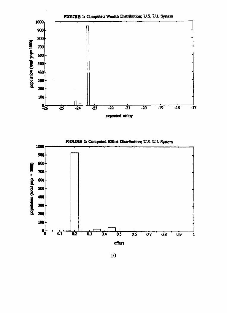
FIGURE 1: Computed Wealth Distribution; U.S. U.L System

900-

h 8fw- % m-

i 600-

0 & soo-

.g 400-

+I 300-

I2 200-

100-

36 -25 n n.,,- -24 -23 s -22 -21 -20 -19 -18 -17

expected utility

1000~ FIOURB 2: Computed Abort Distribution; U.S. U.I. Sywam

7 m-

8 800-

‘;; 700 d B 600-

8 s00

f k

:- & 200-

100-

Oo 0.1 n,r-l- *_..._.

R2 0.3 0.4 0.5 0.6 0.7 0.8 0.9

effort

10

1000

“t - Q

800-

7 ‘O” 6 8L 6oor 3 500- E .g”O -iI loo- B 200-

100 t

OO- . .

FIGURE 3: Computed Consumption Distriiution: U.S. U.L System

I c - I J

1 0.2s 0.3 0.35 0.4 0.45 0.5

consumption

03 FIGURE 4: Effort vs. Wealth; U.S. U.I. System

0.45 - *

0.25 -

0.2 - . . ‘.

1 O*94.1 -24 -23.9 -23.8 -23.7 -23.6 -23.5 -23.4 -23.3

expected utility

11

FIGURE 5: Computed Wealth Distrijution: Autarky

FIGURE 6: Computed Effort Distribution; Autarky

1*1- 900

t

MO L-

Oo 0.1

-23 -22 -21

expected utility

-20 -19 -18 -17

‘1 4 : ! : f - 2 * - - - - - -

I.2 0.3 0.4 0.5 0.6 0.7 0.8 0.9

FIGURE 7: Computed Consumption Distriiution; Autarky

d.600 8 t f no- 2 400- f 300- a & 200-

14

0+ - . 1 0 0.1

I

consumption

RGURE 8: Effort vs. Wealth; Autarky 0.55

0.5 -

0.45 -

a 0.4 -

* 0.35 -

0.3 -

0.25

t

O: 44 3’ . -24.3 -24.2 -24.1 -24 -23.9 -23.8 -23.7 -23.6 .ks

expected utility

13

FIGURE 9: Probability of Re-Employment; U.S. U.I. System

as-

0.8 -

47-

Q6-

0.5 -

a4-

Q3-

0.2 -

0.1 -

OO 1 2 4 6 8 10 12 14 16 18

periods unemployed (plus one)

loo0 FIGURE 10: Computed Wealth Dimtributiun; Optimal System

-23 -22 -21 -20 -19 -18 -17

expected utility

14

Table 1: Comparison of U.S. Unemployment Insurance With Two Alternatives

Mean Effort U. Rate (%) Welfare Gain U.S. U.I. .1966 6.55 0 No U.I. .2133 4.72 - .0031 Autarkv .2219 3.92 -.0115

Figures 5-8 provide some additional information on the autarky solution that can be compared to the content of Figures l-4.

4 Optimal unemployment insurance

In this section, we will suppose that a social planner is free to allocate consumption across agents in each period, contingent on agents’ employment histories. The planner acts to minimize steady state aggregate consumption minus output (the cost of the steady state allocation) subject to the constraint that each new labor-force entrant obtains at least a given level of expected utility. The planner also faces participation constraints,‘j in that the expected utility of each agent cannot fall below what he would receive in autarky. If we let &(.&) d enote the autarkic value of employment (unemployment), we have

Yo = ~$ro(4[u(Y) + PW11+ (1 - ro~4)bP) + Pwol - 4w (1)

Y1 = maxhW[W + P4Ll+ (1 - 7dW40 + PUOl - #W a20 (2)

Let et = 0 if an agent is unemployed in period t of his life, and et = 1 if employed. We will use the convention that et-1 = 0 when t is the date of birth, i.e., young agents are treated as if they were unemployed in the previous period. Then, let ht = (el, e2, . . . . et-r} denote the agent’s employment history at the beginning of period t of life, t = 2,3, . . . . with h’ = (0). Let Ht denote the set of all possible histories to the beginning of period t of life. An unemployment insurance arrangement, 0, is a sequence of functions that map individual histories to individual search effort and current consumption, that is c = {at(ht),st(ht), zt(WL where at ( ht ) is the agent’s recommended search effort in period t, and zt(ht)[zt(h’)] is h is consumption in period t if he is employed [unemployed in period t.

In this private information environment, we wish to determine the optimal unemployment insurance arrangement subject to participation con-

6For similar constraints, see Atkeson and Lucas (1993) or Kocherlakota (1993).

15

straints and incentive compatibility. That is, the unemployment insurance arrangements under consideration are those for which, in each period, each agent prefers the arrangement to autarky, and it is in the interest of each agent to exert the recommended quantity of effort. Given a transversality condition,7 the unimprovability criterion applies. That is, we need only consider one-step deviations, where the agent considers deviating to autarky in the present supposing participation in the future, and considers deviating from the current recommended effort level supposing that they do not devi- ate in the future. Thus, participation constraints and incentive compatibility constraints can be specified in a recursive manner.

Let V(ht+‘)a) d enote the continuation value of the arrangement to the agent, that is, his expected discounted utility at the beginning of period t + 1, conditional on history Iz’+‘, and supposing that the agent carries out the recommended effort levels described in the continuation profile of the contract. An agent has no incentive to leave the unemployment insurance arrangement 0 if, at the beginning of each period, and given any history, the continuation value of the contract is greater than or equal to the expected lifetime utility that he could obtain in autarky. That is, the following participation constraints hold:

WI4 2 L-l 9 (3)

for all t and ht E Ht , where &, i = 1,2, are determined by (1) and (2). Note here that a young agent (new labor-force entrant) faces the same autarkic opportunities as an agent who was unemployed in the previous period. We suppose here that an agent chooses at the beginning of the period whether or not to participate in the unemployment insurance arrangement, then chooses effort. If the agent has chosen to participate, the opportunity to pursue an autarkic employment opportunity is th,en foregone until the following period.

Next, an unemployment insurance contract Q is incentive compatible if

Yet-1 [~t(~t)l(u[~t(ht)l + Psv(iht, lIl”)I +(l - re,-,[ut(ht)]}{[u[zt(ht)] + P~V((ht~O~la)) - #[Wtht)l

2 ret-1 (a’){u[~t(htl + PGV((ht7 lIl”))

(4)

+[l - 7et-l(a’)](?J[zt(ht] + ~~V({ht~O}(~)) - d(a’)

for all a’ 2 0, for all t, and for all ht E Ht. Here, the left side of (4) is the expected discounted utility of the agent if he sets effort at the current recommended level and adheres to the recommended effort levels specified in the continuation profile of the arrangement, conditional on history ht. The right aide of (4) is the expected utility of the agent if he deviates by

7See Green (1987) and Atkeson and Lucas (1992). The transversality condition will be trivially satisfied with upper boundaries on the continuation values of an unemp?oyment insurance arrangement, which will be required for computational purposes.

16

choosing a’ as the current effort level. Note that (4) is a “temporary incentive compatibility” constraint (see Green 1987).

We can think of any unemployment insurance arrangement as represent- ing promises to expected discounted utilities, contingent on employment histories. Let @i denote the set of expected discounted utilities, of an agent with

= i that can be “generated” by an unemployment insurance arrangement ZZtt isf y ing (3) and (4), i.e.,

@p; = {V({h+’ ,i}(o) : CT subject to (3) and (4))

We can establish the following Lemma.

Lemma 1 Qh; = [Ei,v), where v = (1 - /3S)-1[~(~) - #(O)], with U(CG) = Zim,,u(c).

A proof of Lemma 1 is in the Appendix. Note that if the period utility function u(s) is unbounded, then P = 00. Sets @s and @r are important in that, following Spear and Srivastava (1987), history can be summarized by defining the continuation value of the contract to the agent as a state variable, and hence Qi is the space of all admissible expected discounted utilities that can be promised to an agent for whom etml = i, i = 0,l.

We now proceed to transform the problem to a stationary one defined by a set of functions on ai. Specifically, let Pi = (ai( xi(V), zi(V), Vi’(V), Vi*(V) : v E a+}$ = 0,1, where ai( z;(m), zd(.), K1(.), and q*(a) are functions map- ping from @pi to R+,R+, R+, @I, and 9 0, respectively. Here, V E Cpi is a.n admissible state for a type i agent, ai is the effort level of a type i agent [i = 0( 1) if the agent was unemployed (employed) in the previous period] in state V, ei( V)( q(V)) is h is current consumption if currently employed (unemployed), and l$‘(V)(V,‘“‘(V)) ’ h’ t t IS IS s a e next period if he is employed (unemployed) today.

We will call P = (PO, PI) an admissible unemployment insurance rule if

ri[~i(v)lb~~i(v)l + Fww~ (5) +{1 - ri[4v)lm[~i(v)l+ PW”W - #biW

2 %(U’){~[4q + Pw(w +[1 - r;(~‘)](u[Zi(V)l + PWO(V)l - 4w

for i = 0,l for all a’ 1 0, and for all V E <Pi 7 and

V = 7i[G(v)]{"[ai(V)] + PsK'(v)l (6)

+{l - ~i[~i(V)]}{“[zi(V)] + PW*(V)) - +[“i(V)l, for i = 0,l and for all V E Qi. Here, (5) is the stationary counterpart of the incentive constraint (4) and (6) guarantees that expected utility V will be delivered to the agent as promised.

17

An unemployment insurance rule can generate an unemployment insurance contract 6 if at(V) = a,,-,[V(h*la)],z,(ht) = 2,,-1 [V(h”la)], zJht) = a,,_,[V(ht(a)],V((ht,l)Iu) = ~~JV(h*l~)],and V({ht,0)14 = K~-,[V(htld for all t, for all h’ E Ht, and i - 0,l. We then have the following Lemma.

Lemma 2 Let P be any admissible unemployment insurance rule. Then for all V in <PO, an incentive compatible unemployment insurance arrangement u satisfying participation constraints can be generated by P such that V(h’ja) = V.

Lemma 2 permits us to focus on admissible unemployment insurance rules, which we will do for the remainder. To sketch a proof of Lemma 2, and also to see how an unemployment insurance rule works, suppose that a young agent (new labor-force entrant) is born in period 1 and promised some initial level of expected utility vr = V E <PO. At the beginning of period 1, the agent receives a recommendation to choose effort level a(h’) = ao(vl). If the agent becomes employed in period 1, then he receives the consumption allocation z(hl) = zo(vr) and is promised a level of expected utility in period 2 of v2 = V({hl, 1))u) = &yVl). If unemployed, he consumes z(h’) = zo(v1) and is promised v2 = V({hl,O}lo) = q(vr). Next, in period 2, the agent’s recommended action is a,, (v2). Period 2 consumption and period 3 expected utility will then depend only on er, employment status in period 2, and ‘~2. The arrangement then rolls forward until the agent dies, with current effort depending only on promised expected utility at the beginning of the period and last period’s employment status, and consumption and next period’s utility depending only on this period’s expected utility, last period’s employment status, and current employment status.

A key feature of the environment is that the social planner has three incentive devices for eliciting the optima! amount of effort from each agent. First, as in static principal-agent models (e.g., Holmstrom 1979), current compensation can depend on current outcomes, i.e., compensation can be made contingent on current employment status. Second, current compensation can reflect the costs of generating particular outcomes for the agent. That is, given effort, the probability of employment depends on whether or not the agent was employed last period, so consumption should in general be contingent on last period’s employment status, Third, as in other dynamic private information contexts (Green 1987, Spear and Srivastava 1987, Phelan and Townsend 1991, Atkeson and Lucas 1992), future compensation can be used as an incentive device, i.e., future expected utility depends on current and past observed performance.

A key concept that will be used subsequently is the following. A stationary eficient wwmployment insurance rule that delivers expected lifetime utility & to each young agent is an admissible unemployment insurance rule

P such that there exists a probability measure ~1 on @s U <PI and that (P, p) is the solution to the following programming problem which we call (P.l).

min 2 s, hbi(vw-Y + G(V)) + (1 - ril~i(v)]}~i(v)]~~(v) idI ’ subject to ai 2 O,q(V) >, 0,.x@) 2 0, K1(V) E %,&O(V) E @o, (5), (6), and

PC%) = k/ i=o

;v:yl(v)Es ,b+~(v)ld~(v) 1

p(so) = g iv P(V)ESo) 6{1 - 7i[G(V)]}&(V) + (1 - b)r(sO, Vo) (8)

: *

for all S; E Fi, the collection of all Bore1 subsets in a’;, where I( Se, Vo) = 1, if Vo E So; I($, Vo) = 0, otherwise. Thus, the rule is efficient in that it min- imizes the cost of delivering a given level of expected utility to each young agent (note that agents born at different. dates receive the same expected utility) subject to the constraints that the rule be incentive compatible (5) and that promises be kept (6). Al so, the rule is stationary in that the distribution of agents across expected utility states remains constant over time l(7) and @)I-

For convenience, let Ui( V) d enote the expected utility of an agent after current employment status is determined, where i is employment status in the previous period, j is current employment status, and V is promised expected utility at the beginning of the period. We then have

v,‘(V) = U[Zi(V)] - 4[%(V)] + PSv,‘(V), (9) U:(V) = U[S(V)] - d[ai(V)] + @SK’(V),

for i = 0, 1, and for all V E @i. Note that, for an unemployment insurance rule P, if ai = 0 for some

V, then the current probability of employment is Ti[ai(V)] = ri(O) = 0. We can then set U..(V) = U:(V) if ai = 0. We then have the following Lemma.

Lemma 3 Let P be an admissible unemploym.ent insurance rule. Then ai = 0 if and only if Ut( V) = UF( V) and ai( V) > 0 if and only if u;(v) > vi”(V).

The proof of Lemma 3 is straightforward and is in the Appendix. A corollary of Lemma 3 is Ul (V) > UF( V), for all V and i, i.e., contingent on promised expected utility and the previous period’s employment state, an employed agent is better off than an unemployed agent given any admissible

19

unemployment insurance rule. This guarantees that an agent will always accept an employment opportunity.’

In solving problem (P.l) for the stationary efficient unemployment insurance rule, we can successfully deal with the incentive constraints in the problem by using a first-order approach. ’ Here, we will develop conditions under which the first-order approach is valid, and the incentive constraint (5) can be reduced to the equality constraint

for i = 0, 1, and for all V E Oi.

Lemma 4 If u(c) is bounded over [O, 001, then the first-order approach to incentive compatibility is valid.

A proof of Lemma 4 is in the appendix. A similar result can be obtained where U(C) is unbounded.

4.1 Computing solutions to the optimal unemployment insurance problem

In this section we develop an algorithm for computing the stationary efficient unemployment insurance rule defined in the previous section. The first step is to choose discretized approximations to the sets @i, i = 0,l. For each i we let there be n states, so that there are n elements in @pi, i = 0,l. The states are denoted vi(&), k = 1, . . ..n. i = O,l, with wi(k) < vi(k + l), k = 1,2, . ..n - l;~;(l) = &;ui(n) = R, and ui(k + 1) - vi(k) a constant for k = 1,2,...,n - 1. Here & is the expected utility the agent could attain in autarky, and fi is to be chosen (somewhat subjectively) to get the best approximation possible.1°

The state space being finite, the probability measure over the state space 90 U 01 is now a 2n-tuple ~1 = {pi(k) : i = 0,l; k = 1, . . ..n}. where pi(k) denotes the fraction of agents who receive expected discounted utility vi(k) in any period. A stationary efficient unemployment insurance rule is now written

P = (ai(k),~i(k),~i(k),mi(k,l),ni(k,E) : i = O,l;k,l = l,...,p~).

sThis can be contrasted with Atkeson and Lucas (1993), where the key moral-hazard problem has to do with the fact that agents may turn down employment opportunities and this is unobservable,

sThe first-order approach is common in static principa!-agent problems, see Rogerson 1985 but has not been used in dynamic private information problems.

loA higher @ permits agents to attain higher expected utilities and therefore allows for the possibility of larger rewards, but creates a coarser grid, given n.

20

Here ai is the effort level for agents in state t+(k) when employment status in the previous period was i; q(lc) is consumption of agents in state IQ(~) whose previous employment state was i, and who are currently employed; zi( k) is consumption of agents in state vi(K) whose previous employment state was i and who are currently unemployed; md(k, I) is the probability that an agent in employment state i in the previous period who is currently employed and who began the period in state q(k) receives expected utility q( 1) next period; and n;( k, k) is the probability that an agent in employment state i in the previous period who is currently unemployed, and who was promised expected utility ui( k) at the beginning of the period, receives expected utility us(Z) next period. Though expected utilities can only take on values in a discrete set, the problem is convexified here by allowing for lotteries over the promised expected utilities for the following period. Thus, as of the end of the period, the promised expected utility of an agent with current employment status i can take on any value in [vi, VJ.

From the previous section, an admissible unemployment insurance rule P which delivers an ex ante expected discounted utility Vo to each young agent is said to be steady state efficient if there are probability measures ,Y and p = {p(k), k = 1, . . . . n} such that (P, p, p) solve the following programming problem, denoted P.2.

1 n

min c c pi(k)[yi[e(k)][y - +4] + (1 - yi[4k)]M41 i=o kl

subject to:

n

l=l n

+{l - ~~[~i(k)]}{~(~;(k)) + P~~ni(W)vo(O} - 4[41c)lWW7

I=1

dk) = & &&#)]mi(k k),Vk, (13) i=O 1~1

PO(k) = &2{1 - xbi(~)]}w(~9 k)pdk) + (1 - 6)p(k),Vk, (14) i=o I=1

vo = 2 P(k)vo(k) k=l

(15)

21

kp(k) = M(k) 1 O,Vk, (16) k=l

epi(k) = 1;O 6 pi(k) < l,Vi,Vk k=l

(17)

gmi(k,l) = l,Vi;Vk;O 5 mi(k,l) < l,Vk,l - I=1

~~i(k,Z) = l,Vi;Vk;O 5 ni(kyl) < l,Vk,1 - (19) I=1

ai 2 0, xi(k) L: 0, zi(k) L 0, i = 071 (20) Here, equation (11) is the incentive constraint (using the first-order approach), (12) is the promise-keeping constraint, (13) and (14) state that the distribution of agents across expected utility levels is constant over time, (15) states that the expected utility lottery received by young agents gives them an expected utility (before the lottery is executed) of V0 and (16)-(20) are some additional constraints.

Lemma 5 A solution to program P.2 exists.

The proof of Lemma 5 is in the Appendix. Note that our approach here is somewhat different from others in the literature. For example, Phelan and Townsend (1991) assume that effort levels and consumption are chosen from a discrete set, and use lotteries to convert an analogous optimization problem into a linear program. Here, we discretize only over expected utilities, allow consumption and effort to take on values in a continuum, and solve the optimization problem as a nonlinear program. Note also that the optimization problem solves for a steady state distribution of expected utilities across agents, in contrast to other approaches.

4.2 c omputational results and interpretation

Given the functional forms and parameter values from the baseline case, we generated solutions to the programming problem in the previous section. This was done for a range of initial expected utility levels Vo, which in turn generated different minimized cost levels. The results we report are for the level of Vo which produces a minimized cost of zero, i.e., where the government budget balances.

Some summary statistics are provided in Table 2, which can be compared with Table 1. Here, the unemployment rate is 3.15%, which is 3.40 percentage points lower than under the U.S. unemployment insurance system (see Ta- ble 1). Aggregate output is 3.64% higher than with the U.S. unemployment

22

insurance system. This result might be surprising, as one might anticipate that the consumption-smoothing inherent in an optimal unemployment insurance system would be achieved only at the cost of poor incentive effects. However, note that mean effort is higher with the optimal system than with the U.S. unemployment insurance system, and the expected utility of labor- force entrants is much higher. What this indicates is that the current U.S. unemployment insurance system not only has bad consumption-smoothing properties, but also bad incentive effects. What might be even more surprising is that the mean effort level is higher and the unemployment rate lower with the optimal system than in autarky (see Table 1). The autarkic allocation contains the harshest possible penalties for low effort; i.e., consumption is zero when the agent is unemployed. This indicates that the intertemporal incentives built into the optimal contract are important in inducing agents to incur effort costs.

Table 2: Summary Statistics, Optimal System

Mean Effort Unemployment Rate (%) Welfare Gain .2245 3.15 .2073

The welfare gain of new labor-force entrants in the optimal system from the baseline case is very large, exceeding 20% of aggregate consumption (see Table 2). This welfare gain is perhaps implausibly large in that it reflects substantial gains from consumption-smoothing in the optimal system relative to the baseline case, where no consumption-smoothing was possible other than what was provided by the government. The optimal system can be interpreted as involving some mix of government-provided consumption- smoothing and smoothing accomplished through private institutions. A better measure of the welfare gain from optimal unemployment insurance could be obtained if agents could self-insure in the baseline case through private saving (though doing this is beyond the scope of this paper). However, note that this need not reduce the effect of optimal unemployment insurance in lowering the unemployment rate. If agents could self-insure in the baseline case, this would tend to reduce incentives, increasing the baseline unemployment rate and increasing the difference between the baseline unemployment rate and the unemployment rate with the optimal system.

Figures 10 through 24 provide additional data on the characteristics of the optimal unemployment insurance system. Figure 10 shows the distribution of expected utilities across agents in equilibrium, which can be compared to

23

Figures 1 and 5. Note that the optimal system has much more dispersion in wealth than the other two alternatives. Also, more than 70% of the agents in this economy are concentrated at the lower bounds to expected utility, i.e., l/d if unemployed and v, if employed. Transition probabilities are such that any agent will converge to an expected utility path equivalent to autarky in the limit. That is, in the limit each agent’s expected utility follows the same path it would in autarky. However, given that some agents die each period and there are young agents who enter with expected utilities in the upper end of the distribution, there is a stationary distribution of expected utilities which is nondegenerate. In models such as Atkeson and Lucas (1993), where agents are infinite-lived, the limiting wealth distribution is degenerate.

The greater dispersion in the distribution of expected utilities in the optimal system relative to the U.S. U.I. system represents better incentives, in the sense that there are greater opportunities for reward and punishment. We can observe the effects of better incentives in the distribution of effort in Figure 11, as compared to Figure 2. The mean level of effort is higher (Tables 1 and 2), and the optimal effort distribution appears to be better than that achieved with U.S. U.I. in terms of first-order stochastic dominance.

As with wealth, the distribution of consumption across agents has more dispersion in the optimal system (Figure 12) than with U.S. U.I. (Figure 3). A significant fraction of agents in the population consume zero, and the highest level of consumption is almost double the output produced by an employed agent (output per employed agent is .2). The large dispersion in consumption reflects the use of current compensation as an incentive device, relative to the use of future compensation (as reflected in the wide dispersion in expected utilities).

Figure 13 shows that, for unemployed agents, effort as a function of expected utility level is an inverted U. Unemployed agents in the middle of the wealth distribution face stiff penalties in remaining unemployed and high rewards in gaining employment, in terms of future compensation. That is, their expected utility level can fall by a large amount or increase by a large amount. When agents reach the minimum level of expected utility, intertemporal penalties become inoperative, and for agents at the top of the wealth distribution, intertemporal rewards are very costly. In Figure 13, the profile for employed agents is quite flat. That is, intertemporal penalties and rewards play almost no role in inducing employed agents to choose optimal effort.

Some key features of the optimal system are illustrated in Figures 14 and 15. In the Figure, (k, I) denotes an agent whose employment status is k this period and was 1 last period. For example (1,0) denotes an agent who is employed this period and was unemployed last period. As one might anticipate, conditional on employment status last period, an agent consumes more

24

FIGURE 11: Computed Effort Distriiution; Optimal System

3 500- i!. 0 400-

fi & 300-

& 200-

100 t

OO 0.1 0.2 0.3 0.4 0.5 0.6 0.7 0.8

effon

FIGURE 12: Computed Consumption Distribution; Optimal System

900 t

-800 3 ‘;; ‘O” k600 & / 3 soo- Ee .I 400- GJ 300-

!z 200-

1:, 0 0.1

*

consumption

25

FIGURE 13: EBort vs. Wealth; Optimal System 1

Q9-

0.8-

Q7-

a6- *.-- ..-- _.-- ..-- --~---~-*\ ..,.,

OS- .--- /- -.--

‘A _.-- -3” a4-

a3-

emplayed

-22 -21 -20 -19 -18

expected utility

PiGUN 14: Cmsumptian vs. Weauh; Optimal Symm

expected utility

26

FIGURE 15: Future Wealth vs. Current Wealth; Optimal System

expected utility in period t

0.3 FIGURE 16: Consumption of Unemployed

0.25 -

0.2 -

s t 0.15 - I 8

0.1 -

0.05 -

OO 2 4 -

6 8 10 12 14 16 18 20


27

FIGURE 17: Rcphuemnt Ratio FIGURE 17: Rcphuemnt Ratio

perioda unemployed (plus one)

as5 FIGURE 18: Effor& of the Unemployed

as -

OAS-

P a4-

u a35 -

a3-

oa-

a2O I 2 4 6 8 10 12 14 16 18

periods unemployed

1

28

FIGURE 19: Probability of Re-Employmcnq Optimal System 1

r 0.9 -

0.8 -

0.7 -

0.6 -

a5 -

Q4-

0.3 -

0.2 -

0.1 -

t OO 2 4 6 8 10 12 14


I 16 18 20

-20 -

-21 -

-22 -

-23-

-24 -

-% 2 4 6 8 10 12 14 16 18 20

periods unemployed

29

Q22-

3 O** @ a18- I s 0.16-

0.14 -

0.12 -

FIGURE 21: Consumption of the Employed

I

a1O 2 4 6 8 10 12 14

periods of smployment (plus one)

I

16 18 20

a55 1 FIGURE 22: Effort of the Employed

1

0.3 -

0.45 -

a

084-

o Q35-

0.3 -

0.2s -

L &a, 2 4 6 8 10 12 14

periods of unemployment (plus one)

I 16 18 20

30

1

0.9 -

0.8 -

0.7 -

PIGURE 23: Probability of Employment for the Emplayed

B O-6 -

f/ 0.5 -

a 0.4 -

0.3 -

0.2 -

0.1 -

OO 2 4 6 8 10 12 14 16 18 20

periods of employment (plus one)

-228 FIGURE 24 Wealth of the Employed I

$ -23 -

3 -23.1-

ii o -23.2-

periods of employment (plus one)

when employed than when unemployed. Also, consumption is monotonically increasing with the expected utility promised to the agent, conditional on this period’s and last period’s employment status. What might be surprising is that an employed agent consumes more if he was unemployed last period than if he was employed, and an unemployed agent consumes more if he was unemployed last period than if he was employed. Thus, there is a large reward for a transition from unemployment to employment, and a large penalty for a transition from employment to unemployment. Figure 15 tells a very similar story; again there are large rewards and penalties, here in terms of future compensation, for labor-market transitions. Note here that the profile for an agent who was employed this period and last period is very close to the 45” line. That is, the expected utility of an agent who remains employed does not change much, on average. However, unemployed agents tend to move down in the wealth distribution, and an unemployed agent who becomes employed tends to move up.

The incentives built into the optimal system affect the effort choices of the employed and unemployed, but tend to have a greater effect on the employed. Effort of the employed increases on average in the optimal system by 18.5% over the baseline case (U.S. U.I.) and by 12.1% on average for the unemployed. For these results to be taken seriously, it must be the case that moral hazard is an important feature of a significant fraction of worker- management relationships. More than twenty years of work on principal- agent models argues that this is the case.

One feature of the unemployment insurance system that we would like to examine here is the consumption path followed by an agent who is employed and then becomes unemployed for a large number of consecutive periods, This would provide a useful comparison with results in Shave11 and Weiss (1979) and Hopenhayn and Nicolini (1995). A problem in making this comparison is that an agent’s consumption path will be stochastic, even if her employment status stays constant due to the expected utility lotteries. To make a comparison we consider an employed agent with the highest expected utility, and suppose that the arrivals of stochastic employment opportunities are such that he is unemployed for 20 consecutive periods. We generated consumption profiles in 3.00 experiments, and then averaged across these experiments to obtain Figure 16. This is then close to the average experience of an unemployed agent. It is perhaps more useful to study the path of the replacement ratio (consumption divided by consumption in the last period of employment) in Figure 17. Period 1 is the last period of employment, and the agent is unemployed for periods 2 through 20. An important feature of the profile is that it is not monotonic, as in Shave11 and Weiss (1979) and Hopenhayn and Nicolini (1995). The difference here is that we account for labor-market transitions. That is, since there is a large penalty for a transi-

32

tion from employment to unemployment, the agent consumes less in the first period of unemployment than in the second, and consumption declines monotonically thereafter. Figure 17 indicates much more consumption-smoothing than in the U.S. U.I. system, where unemployment compensation is received for only two quarters. Here, the replacement ratio falls below l/2 only after 5 quarters of unemployment. The initial replacement ratio is quite high here. It is over 80% in the first period of unemployment and it exceeds 90% in the second. The U.S. U.I. system generates a replacement ratio of about 2/3 for two quarters.

Figure 18 shows the corresponding average effort-level profile for an agent employed in period 1 and unemployed for periods 2 through 20. Here, effort increases as the a,gent becomes unemployed, and it is higher in the earlier part of the unemployment spell than in the later part. The effects of the effort profile can also be seen in Figure 19, which shows the probability of reemployment. Note how this compares to Figure 9 for the U.S. U.I. system, where effort is lower early in the unemployment spell and higher later. It is the large rewards to reemployment in the optimal system - essentially a subsidy which is paid when an unemployed agent gets a job - which generate an incentive to choose high search effort early in the unemployment spell.

Figure 20 shows the average behavior of wealth for an unemployed agent. Here, expected utility declines monotonically to the autarkic level. Note that expected utility does not have the same nonmonotonicity as does the path for consumption in Figure 16. That is, in the period the agent became unemployed effort was low, and effort rises in the following period. Thus, the nonmonotonicity in the consumption path (Figure 16) mirrors the nonmonotonicity in effort (Figure 18), generating aP monotonic path for expected utility (Figure 20).

Figures 21 through 24 show what, on average, happens to an initially unemployed agent who is near the bottom of the wealth distribution, becomes employed in period 2, and remains employed thereafter. There is a large consumption bonus when reemployment occurs and then consumption is virtually flat thereafter (Figure 21). In this case, there is a small tax on employed workers (consumption slightly less than output, which is .2). Effort drops on employment and remains flat thereafter (Figure 22), and expected utility tends to drift downward over time (Figure 24).

5 Summary and conclusion

We have studied a dynamic model with moral hazard where agents face stochastic production opportunities, and the probability of employment each period depends on unobservable effort. Given effort, the probability of employment this period is higher if the agent was employed last period. In this

33

environment, there is a tradeoff between the consumption-smoothing benefits provided by unemployment insurance and the costs, which take the form of reduced search effort of the unemployed and lower effort on the job.

Our numerical work shows that an optimal unemployment insurance system which fully utilizes intratemporal and intertemporal incentives can reduce the unemployment rate by 3.40 percentage points and increase aggregate output by 3.64% relative to the unemployment insurance system currently in place in the United States. The practical application of such an optimal system in the United States would involve individual experience rating of workers. Essentially, a worker would have an individual unemployment insurance “account” which would summarize his employment history and determine taxes (or transfers) when employed and benefits when unemployed. Key features of the program are that workers receive a subsidy when they become employed after a spell of unemployment, and that benefits initially rise during an unemployment spell and then decline monotonically. The im- plementation of such an unemployment insurance program would appear to be feasible.

The model here could be extended in a number of directions, including the following three. First, it would be interesting to incorporate adverse selection, given that firm-level experience rating in the United States seems to be intended to mitigate an adverse selection problem. That is, the government finds it difficult or impossible to distinguish between unemployed workers who are on temporary layoff and those who are permanently separated. Firm-level experience rating forces the firm to bear the costs of temporary layoffs. Our model could be modified to include adverse selection by giving some of the unemployed a higher probability of reemployment, given effort, than other unemployed agents. Given this, one of the likely effects would be to reduce the subsidy paid on reemployment, since this subsidy would tend to encourage temporary layoffs. This said, moral hazard appears to be the primary information friction associated with unemployment insurance. Clearly, moral hazard for unemployed workers is a serious problem, and the work effort of the employed is only imperfectly monitored by firms in many contexts. Even if experience rating gives the firm the,incentive to reveal what it knows about workers’ effort, the firm’s information may be limited,

Second, in principle the model could be extended to allow for self-insurance, at least through some blunt mechanism such as permitting agents to accu- mulate assets, but still restricting borrowing against future income. In that kind of environment, rewards and penalties in terms of current payments to agents would not have as much force (if wealth were unobservable), since agents could use savings to smooth consumption in the face of these rewards and penalties. A problem with this approach is that allowing for savings would make the model much more difficult to solve. In defense of the no-

34

savings assumption in our model, the ability of the unemployed to smooth consumption from quarter to quarter may be quite limited due to the inability to borrow and the illiquidity of wealth (in particular, consumer durables and housing).

Third, one could allow production opportunities to be drawn from a fixed distribution, as in rnodels of one-sided search, and thus generate the possibility that wage offers could be rejected. This would permit a more detailed study of the effects of unemployment insurance on the distribution of income and wealth.

35

Appendix

Proof of Lemma 1. Consider an unemployment contract which pays a constant benefit 8 E [O, oo] every period from period t, no matter whether the agent is employed or not. Such an unemployment contract will generate a constant expected life-time utility for a type i agent:

i = 0,l. It is straightforward to show that K(0) is continuous, and E(O) = JL, &(oo) = P. So for each V E [vi, V), there is some 8 such that K(0) = V. The Lemma is proven.

Proof of Lemma 3. Fix i and V. Suppose U;(V) = UT(V), then obviously ai = 0 is the only incentive compatible effort.

Next, let ai( V) > 0 and let 0 < a’ < ai( V). Manipulation of constraint (5) gives,

(r[%(v)] - Y(QI)}[u/(V) - K'(V)] L 4[“i(V)l- #(a’)*

But 7[q(V)] > I and qb[ui(V)] > #(a’), hence U:(V) > U:(V). Finally, suppose Ut (V) > U!(V). If ui( V) = 0, we then have Ut (V) =

U,f’( V), a contradiction. Therefore, ui(V) > 0 and the Lemma is proven.

Proof of Lemma 4. Let P be any unemployment insurance plan that satisfies incentive constraint (5). We show that constraint (1) must then hold. For an agent in state V, who takes action a in the current period, expected discounted utility can be written as

G;(a) = [u/(V) - u.(V)]?(u) - +(a) + u(~i(V)) + @V;‘(V). Notice that U/(V) - U.(V) does not depend on a. Therefore,

G;(u) = [U;(V) - U;(V)]&) - t#‘(u),

G;(u) = [U/(V) - Uf(V)]ri”(u) - #‘l(u) By Lemma 3, we know that U:(V) 1 U?(V). Suppose U:(V), then given

Lemma 3, Q;(V) = 0, and (10) is satisfied. Next, suppose U/(V) > U..(V). Then G:(u) < 0 given that 7i(*) is strictly concave and d(g) is strictly convex. We also have G:(O) > 0, and lim 0ti03G:(a) < 0. Therefore, G;(c) attains a unique maximum for some unique a*, with 0 < a* < 00, where Gl(A.*) = 0, and (10) is satisfied.

Next, suppose (10) is true. If u;(V) = 0, then ~,4’[ai(V)] = 0 and hence u:(V) = U:(V) and (5) is satisfied. If q(V) > 0, then d’[ui(V)] > 0 and

36

by (10) we have U:(V) > U?(V). But th’ 1s in turn implies Gi(a) is strictly concave. Moreover, given the above, G:(O) > O,lim,,,G:(a) < 0, so (10) is necessary and sufficient for global maximization. But ai solves (10) so it must satisfy (5). The Lemma is proven.

Proof of Lemma 5. First, we look at the case where u(c) is bounded over [O,oo]. Let z& = u[;c~(~)],u:~ = u[z;(k)], and let u-l -be the’ inverse function of u. *Then problem P.2 can be transformed intd the following. Choose a;(~),u~(~),nzi(~, Z),ni(L,Z),pi(L),i = 0,1, j = O,l, A$1 = 1,2, . . . . n, to solve

subject to:

?.& + ps&72i(k,z)q(z) - uyk - p&ni(k,z)Vo(l) = fI$;;,vi,vk, I=1 I=1 i i

+{l -7i[“i(k)]}[U$ + P~~ni(k,z)~O(z)] - +[%(~)],~~,~~y 1

(13)-( 19), and 0 < c&(k) 5 ii,0 5 u& 5 u(oo),Vk, j, k

Here, a is some sufficiently large upper bound on ui(k). The above minimiza- tion problem has a continuous objective function and a compact constraint set, and therefore has a solution.

Second, we consider the case where u(c) is unbounded over 10, oo]. Sup- pose problem P.2 does not have a solution. For each integer N > 0, replace constraint (19) in program P.2 by

a;(k) > 030 5 xi(k) < NY0 5 z;(k) 5 N,

and call the resulting programming problem P.2N. For each N, P.2N can be transformed into a problem which has a continuous objective function and a compact constraint set and hence a solution exists. Denote this solution by PN = (u~(k),x~(k),z~(k),mlv(k,Z)i = 0.1; k,Z = l,...,n}. Nonexistence of a solution to P.2 implies that there is an i and k such that either x:(k) = N or z:(k) = N. Moreover, this is an i, a k, and a subsequence {Np)zl of

UwLl such that either x?(k) + 00 or Zi Nq (4 + 00, as Q + 00. Suppose ziyq 3 00 is the case. Since u(c) is unbounded,

u[zF(k)] + ,&i~nNq(k,Z)vO(Z) + 00, as q + 00 1

37

But by Lemma 3,

?.+yyk)] + PSE mNq(k, E)q(l) ,> u[gyk, k)vo(l) 1

Therefore, we also have

+iN’(k)l + Pbx mNq(k, l)wl + 00 as q -+ oo 1

and constraint (12) is violated. Next, suppose x?(k) -t oo is the case. Then for constraint (12) to hold it must be true that a?(k) + 0, and hence fbe?( k)] --) 0, as q ---) -. But then from the incentive constraint (ll), we

l;m,,,{+f%)] + PS x nNq(k, +,(l)} 1

again contradicting (12). The Lemma is proven.

38

References

Abowd, J. and Zellner, A., (1985). Estimating Gross Labor-Force Flows, Journal of Business and Economic Statistics, 3: 254-283.

Albrecht, J. and Axell, B., (1984). An Equilibrium Model of Search Unem- ployment, Journal of Political Economy, 92: 824-840.

Atkeson, A. and Lucas, R., (1992). ON Efficient Distribution With Private Information, Review of Economic Studies, 59: 427-453.

Atkeson, A. and Lucas, R., (1993). Efficiency and Equality in a Simple Model of Efficient Unemployment Insurance, NBER working paper 4381.

Avrutis, R., (1983). H ow to Collect Urxmployment Benefits: Complete In- formation for All 50 States, Prentice-Hall, Englewood Cliffs, NJ.

Bl.anchard, 0. and Diamon, P., (1990). The Cyclical Behavior of the Gross Flows of U.S. Workers, Brookings Papers on Economic Activity, 2.

Clark, K. and Summers, L., (1983). U nemployment Insurance and Labor Market ‘Transitions, M. Baily (ed.) Workers, Jobs and Inflation, 279-316. Brookings Institution, Washington, D.C.

Green, E., (1987). Lending and the Smoothing of Uninsurable Income, E. Prescott and N. Wallace, (eds.). Contractual Arrangements for Intertempo- ml Trade, University of Minnesota Press, Minneapolis, MN.

Hansen, G. and Imrohoroglu, A., (1992). The Role of Unemployment Insur- ance in an Economy with Liquidity Constraints and Moral Hazard, Journal of Political Economy, 100: 118-142.

Hansen, L. and Byers, J., 91990). Unemployment Insurance: The Second Half Century, University of Wisconsin Press, Madison, WI.

Holmstrom, B., (1979). Moral Hazard and Observability, Bell Journal of Economics, 10: 74-91.

Hopenhayn, H. and Nicolini, J., (1995). Optimal Unemployment Insurance, working paper,University of Rochester, Universitat Pompeu Fabra, and Uni- versidad ‘Torcuato Di Tella.

39

Kocherlakota, N., (1993). Efficient Bilateral Risk Sharing Without Commit- ment, working paper, Uaiversity of Iowa.

Mortensen, D., (1977). Unemployment Insurance and Job Search Decisions, Industrial and Labor Relations Review, 30: 505-517.

Mortensen, D., (1983). A W If e are Analysis of Unemployment Insurance: Variations on Second-Best Themes, Carnegie-Rochester Conference Series on Public Policy, 19: 67-98.

Phelan, C., (1994). Incentives and Aggregate Shocks, Review of Economic Studies, 61: 681-70Q.

Phelan, C. and Townsend, R., (1991). Computing Multi-Period Information- Constrained Optima, Review of Economic Studies, 58: 853-881.

Rogerson, W., (1985). The First-Order Approach to Principal-Agent Prob- lems, Econc,metrica, 53: 1357-1368.

Shave& S. and Weiss, L, (1979). The Optimal Payment of Unemployment Insurance Benefits Over Time, Journal of Political Economy, 87: 1347-1362.

Spear, S. and Srivastava, S., (1987). On Repeated Moral Hazard With Dis- counting, Review of Economic Studies, 54: 599-618.

Taub, B., (1990). The Equivalence of Lending Equilibria and Signalling Based Insurance Under Asymmetric Information, Rand Journal of Economics, 23: 388-408.

Topel, R., ( 1984). Experience Rating of IJnemployment Insurance and the incidence of Unemployment, Journal of Law and Economics, 27: 61-99.

Topel, R., (1990). F’ mancing Unemployment Insurance: History, Incentives, and Reform, W. Hansen and J. Byers, (eds.). Unemployment Insurance: The Second Half-Century, University of Wisconsin Press, Madison, WI.

United States Congress. (1993). 1993 Green Book; Overview of Entitlement Pmgrams. U.S. House of Representatives, Committee on Ways and Means,

Wang, C., (1994). Incentives, CEO Compensation, and Shareholder Wealth in a Dynamic Agency Model, working paper, Carnegie Mellon University.

40

Wang, C., (1995). Dy namic Insurance with Private Information and Bal- anced Budgets, forthcoming, Review of Economic Studies.

Zhang, C., (1995). U nemployment Insurance Analysis in a Search Economy, working paper, University of Rochester.

41

unemployment insurance with moral hazard ... - penn...

Documents