Unemployment (Fears) and Deflationary Spirals

Wouter J. Den Haan, Pontus Rendahl, and Markus Riegler†

September 24, 2015

AbstractThe interaction of incomplete markets and sticky nominal wages is shown to magnifybusiness cycles even though these two features – in isolation – dampen them. Duringrecessions, fears of unemployment stir up precautionary sentiments which inducesagents to save more. The additional savings may be used as investments in botha productive asset (equity) and an unproductive asset (money). But even a smallrise in money demand has important consequences. The desire to hold money putsdeflationary pressure on the economy, which, provided that nominal wages aresticky, increases wage costs and reduces firm profits. Lower profits repress the desireto save in equity, which increases (the fear of) unemployment, and so on. This isa powerful mechanism which causes the model to behave differently from bothits complete markets version, and a version with incomplete markets but withoutaggregate uncertainty. In contrast to previous results in the literature, agents uniformlyprefer non-trivial levels of unemployment insurance.

Keywords: Keynesian unemployment, business cycles, search friction, magnification,propagation, heterogeneous agents.JEL Classification: E12, E24, E32, E41, J64, J65.

†Den Haan: London School of Economics, CEPR, and CFM. E-mail: wjdenhaan@gmail.com. Rendahl:University of Cambridge, CEPR, and CFM. E-mail: pontus.rendahl@gmail.com. Riegler: University ofBonn and CFM. E-mail: mriegler@uni-bonn.de. We would like to thank Chris Carroll, Zeno Enders, GregKaplan, Per Krusell, Kurt Mitman, Michael Reiter, Rana Sajedi, Victor Rios-Rull, and Petr Sedlacek, for usefulcomments. The usual disclaimer applies.

1 Introduction

The empirical literature documents that workers suffer substantial losses in both earningsand consumption levels during unemployment. For instance, Kolsrud, Landais, Nilsson,and Spinnewijn (2015) use Swedish data to document that consumption expenditures dropon average by 32% during the first year of an unemployment spell.1 This observed inabil-ity to insure against unemployment spells has motivated several researchers to developbusiness cycle models with a focus on incomplete markets. The hope (and expectation)has been that such models would not only generate more realistic behavior for individualvariables, but also be able to generate volatile and prolonged business cycles withoutrelying on large and persistent exogenous shocks. While in existing models, individualconsumption is indeed much more volatile than aggregate consumption, aggregate vari-ables are often not substantially more volatile than their counterparts in the correspondingcomplete markets (or representative-agent) version. Krusell, Mukoyama, and Sahin (2010),for instance, find that imperfect risk sharing does not help in generating more volatilebusiness cycles. McKay and Reis (2013) document that a decrease in unemploymentbenefits – which exacerbates market incompleteness – actually decreases the volatility ofaggregate consumption.2 The reason is that an increase in unemployment benefits reducesprecautionary savings, investment, the capital stock, and ultimately makes the economy asa whole less well equipped to smooth consumption.

We develop a model in which the inability to insure against unemployment risk gen-erates business cycles which are much more volatile than the corresponding completemarkets version. Moreover, although the only aggregate exogenous shock has a smallstandard deviation, the outcome of key exercises such as changes in unemployment bene-fits depends crucially on whether there is aggregate uncertainty. This result is obtainedby combining incomplete asset markets with incomplete adjustments of the nominalwage rate to changes in the price level.3 The impact of shocks is prolonged by Diamond-Mortensen-Pissarides search frictions in the labor market.

Before explaining why the combination of incomplete markets and sticky nominalwages amplifies business cycles, we first explain why these features by themselves dampenbusiness cycles in our model in which aggregate fluctuations are caused by productivityshocks. First, consider the model in which there are complete markets, but nominal wages

1Section 3.2 provides a more detailed discussion of the empirical literature investigating the behavior ofindividual consumption during unemployment spells.

2As discussed in section 7.1, a decrease in unemployment benefits does increase the volatility of output inthe model of McKay and Reis (2013), but the effects are small relative to our results.

3We discuss the empirical motivation for these assumptions in section 3.

1

do not respond one-for-one to price level changes. A negative productivity shock operateslike a negative supply shock which puts upward pressure on the price level. Providedthat nominal wages are sticky, the resulting downward pressure on real wages mitigatesthe reduction in profits caused by the direct negative effect of a decline in productivity.The result is a muted aggregate downturn. Next, consider a model in which nominalwages are flexible, but workers cannot fully insure themselves against unemploymentrisk. Forward-looking agents understand that a persistent negative productivity shockincreases the risk of being unemployed in the near future. If workers are not fully insuredagainst this risk, the desire to save increases for precautionary reasons. However, increasedsavings leads to an increase in demand for all assets, including productive assets such asfirm ownership. This counteracting effect alleviates the initial reduction in demand forproductive assets, induced by the direct negative effect of a reduced productivity level and,therefore, dampens the increase in unemployment. In either case, sticky nominal wages orincomplete markets lead – in isolation – to a muted business cycle.

Why does the combination of incomplete markets and sticky nominal wages lead tothe opposite results? As before, the increased probability of being unemployed in thenear future increases agents’ desire to save more in all assets. However, the increaseddesire to hold money puts downward pressure on the price level, which in turn increasesreal wage costs and reduces profits. This latter effect counters any positive effect thatincreased precautionary savings might have on the demand for productive investments.Once started, this channel will reinforce itself. That is, if precautionary savings lead –through downward pressure on prices – to increased unemployment, then this will in turnlead to a further increase in precautionary savings, and so on. When does this processcome to an end? At some point, the nonlinearities in the matching function, combined withan expanding number of workers searching for a new job, makes it attractive to resumejob creating investments.

In addition to endogenizing unemployment, the presence of search frictions in thelabor market adds further dynamics to this propagation mechanism. First, the value of afirm – i.e. the price of equity – is forward-looking. As a consequence, a prolonged increasein real wage costs leads to a sharp reduction in economic activity already in the present,with an associated higher risk of unemployment. Second, with low job-finding ratesunemployment becomes a slow moving variable. Thus, the increase in unemployment ismore persistent than the reduction in productivity itself.

We use our framework to study the advantages of alternative unemployment insurance(UI) policies. We first document that the effects of changes in unemployment benefitson the behavior of aggregate variables and on the well-being of workers differ from the

2

effects in other models. For example, in the model of Krusell, Mukoyama, and Sahin (2010)most agents benefit from reductions in unemployment benefits even when benefits arereduced to very low levels. We consider a permanent increase in the replacement rate fromthe benchmark value of 50% of the prevailing wage rate to 55% and document that thisincrease in insurance improves the welfare of all agents, provided that the policy switchoccurs in a recession. This is true even if wage rates adjust upwards to take into accountthe strengthened bargaining position of workers.4

There are a number of factors affecting agents’ welfare that are important for this result.As a preview of the analysis, let us mention some that operate in our model, but have notbeen previously emphasized in the literature. Consider a permanent increase in unemploy-ment benefits at the onset of a recession. This obviously benefits the unemployed directly.But the employed benefit too. Firstly, they benefit because they are better insured againstfuture unemployment risk. Secondly, by reducing the negative downward spiral discussedabove, the employed are now less likely to be unemployed in the near future. Thirdly, andperhaps more surprisingly, employed agents also benefit because the dampening of thedownward spiral implies that the value of their asset holdings drops less relative to thecase in which unemployment benefits are not increased.

These features contrast with those exposed in the existing literature, in which increasedunemployment benefits brings forth adverse aggregate consequences that eclipse the gainsof reduced income volatility (e.g. Young (2004) and Krusell, Mukoyama, and Sahin (2010)).In particular, with lower fluctuations in individual income the precautionary motiveweakens, and aggregate investment falls. The result is a decline in average employmentand output, with adverse effects on welfare. This channel is important in our model aswell. In the version of our model with aggregate uncertainty, however, there are twoquantitatively important factors that push average employment in the opposite direction,and can overturn the negative effect associated with the reduction in precautionary savings.The first is that the demand for the productive asset can increase, because an increase in thelevel of unemployment benefits stabilizes business cycles and asset prices. The second isthat the nonlinearity in the matching process is such that increases in employment duringexpansions are smaller than reductions during recessions. Consequently, a reduction involatility can lead to an increase in average employment (cf. Jung and Kuester (2011)).

An important aspect of our model is that precautionary savings can be used for invest-ments in both the productive asset (firm ownership) and the unproductive asset (money).This complicates the analysis, because the numerical procedure requires a simultaneous

4Wage increases reduce job creation which has negative welfare consequences. Whether all agents preferthe switch during an expansion depends crucially to which extent wages adjust.

3

solution for a portfolio choice problem for each agent, and for equilibrium prices. Ournumerical analysis ensures that the market for firm ownership (equity) is in equilibriumand all agents owning equity discount future equity returns with the correct, that is, theirown individual-specific, intertemporal marginal rate of substitution (MRS).5 By contrast, atypical set of assumptions in the literature is that workers jointly own the productive assetat equal shares, that these shares cannot be sold, and that discounting of the returns ofthis asset occurs with some average MRS or an MRS based on aggregate consumption.6,7

One exceptions is Krusell, Mukoyama, and Sahin (2010)who – like us – allow trade in theproductive asset and discount agents’ returns on this asset with the correct marginal rateof substitution.8

In section 2, we describe the model. In section 3, we provide empirical motivation forthe key assumptions underlying our model: sticky nominal wages and workers’ inability toinsure against unemployment risk. We also discuss the relationship between savings andidiosyncratic uncertainty. In section 4, we discuss the calibration of our model. In sections5 and 6, we describe the behavior of individual and aggregate variables, respectively. Insection 7, we discuss how business cycle behavior is affected by alternative UI policies.

2 Model

The economy consists of a unit mass of households, a large mass of potential firms, and onegovernment. The mass of active firms is denoted qt, and all firms are identical. Householdsare ex-ante homogenous, but differ ex-post in terms of their employment status (employedor unemployed) and their asset holdings.

Notation. Upper (lower) case variables denote nominal (real) variables. Variables withsubscript i are household specific. Variables without a subscript i are either aggregatevariables or variables that are identical across agents, such as prices.

5See section 2.7 for a detailed discussion.6Examples are Shao and Silos (2007), Nakajima (2010), Gorneman, Kuester, and Nakajima (2012), Favilukis,

Ludvigson, and Van Nieuwerburgh (2013), Jung and Kuester (2015), and Ravn and Sterk (2015).7An alternative simplifying assumption is that the only agents who are allowed to invest in the productive

asset are agents that are not affected by idiosyncratic risk (of any kind). Examples are Rudanko (2009), Bils,Chang, and Kim (2011), Challe, Matheron, Ragot, and Rubio-Ramirez (2014), and Challe and Ragot (2014).Bayer, Luetticke, Pham-Dao, and Tjaden (2014) analyze a more challenging problem than ours, in whichfirms are engaged in intertemporal decision making. However, in contrast to our model, these firms areassumed to be risk neutral, consume their own profits, and discount the future at a constant geometric rate.

8The procedure in Krusell, Mukoyama, and Sahin (2010) is only exact if the aggregate shock can take onas many realizations as there are assets and no agents are at the short-selling constraint. Our procedure doesnot require such restrictions, which is important, because the fraction of agents at the constraint is nontrivialin our model.

4

2.1 Households

Each household consists of one worker who is either employed, ei,t = 1, or unemployed,ei,t = 0. The period-t budget constraint of household i is given by

Ptci,t + Jt (qi,t+1 − (1− δ) qi,t) + Mi,t+1

= (1− τt)Wtei,t + µ (1− τt)Wt (1− ei,t) + Dtqi,t + Mi,t, (1)

where ci,t denotes consumption of household i, Pt the price of the consumption good, Mi,t

the amount of the liquid asset held at the beginning of period t (chosen in period t− 1), Wt,the nominal wage rate, τt the tax rate on nominal income, and µ the replacement rate. Thevariable qi,t denotes the amount of equity held at the beginning of period t. Equity pay outnominal dividends Dt. In each period, a fraction δ of all firms go out of business whichleads to a corresponding loss in equity.9 When the term qi,t+1 − (1− δ) qi,t is positive, theworker is buying equity, and vice versa. The nominal value of this transaction is equal toJt (qi,t+1 − (1− δ) qi,t), where Jt denotes the nominal price of equity ex dividend.

Households are not allowed to take short positions in equity, that is

qi,t+1 ≥ 0. (2)

The household maximizes the objective function10

Et

∞

∑j=0

βj

c1−γi,t+j − 1

1− γ+ χ

(Mi,t+1+j

Pt+j

)1−ζ− 1

1− ζ

,

subject to constraints (1) and (2).The first-order conditions are given as

c−γi,t = βEt

[c−γ

i,t+1Pt

Pt+1

]+ χ

(Mi,t+1

Pt

)−ζ

, (3)

c−γi,t ≥ βEt

[c−γ

i,t+1

(Dt+1 + (1− δ) Jt+1

Jt

)Pt

Pt+1

], (4)

0 = qi,t+1

(c−γ

i,t − βEt

[c−γ

i,t+1

(Dt+1 + (1− δ) Jt+1

Jt

)Pt

Pt+1

]). (5)

9We assume that households hold a diversified portfolio of equity, which means that the porfoliodepreciates at rate δ.

10If money and consumption enter the utility function additively, then money does not enter the Eulerequation of other assets directly, which is consistent with the empirical results in Ireland (2004).

5

Equation (3) represents the Euler equation with respect to real money balances; equation(4) the Euler equation with respect to equity; and equation (5) captures the complementaryslackness condition associated with the short-selling constraint in equation (2).

Telyukova (2013) documents that households hold more liquid assets than they needfor buying goods. This is consistent with our model, in which agents do not only holdmoney to facilitate transactions, but also to insure themselves against unemployment risk.The utility specification implies that agents will always choose a positive value of realmoney balances. Short positions in the liquid asset would become possible if the argumentof the utility function is equal to (Mi,t + Φ)/Pt with Φ > 0 instead of Mi,t/Pt. At highervalues of Φ, agents can take larger short positions in money and are, thus, better insuredagainst unemployment risk. Increases in χ – while keeping Φ equal to zero – have similarimplications, since higher values of χ imply higher average levels of financial assets.

2.2 Active firms

An active firm produces zt units of the output good in each period, where zt is an exogenousstochastic variable that is identical across firms. The value of zt follows a first-order Markovprocess with a low (recession) and a high (expansion) value. The partition into a recessionand an expansion regime simplifies the characterization of the model’s properties.11

There is one worker attached to each active firm. Thus, the number of active firms, qt,is equal to the economy-wide employment rate. The nominal wage rate, Wt, is the onlycost to the firm. Consequently, nominal firm profits, Dt, are given by

Dt = Ptzt −Wt. (6)

The nominal wage rate is set according to the rule

Wt = ω0

(zt

z

)ωzz(

Pt

P

)ωP

P, (7)

where z is the average productivity level, Pt is the price level, and P is the average pricelevel.12 A key aspect of this paper is on the responsiveness of nominal wages, Wt, tonominal prices, Pt. Therefore, we need a wage setting rule which allows us to vary this

11Although the model is solvable for richer processes, this simple specification for zt helps in keeping thecomputational burden manageable.

12The specified wage is always in the worker’s bargaining set, since the wage rate exceeds unemploymentbenefits, there is no home production nor any disutility from working, and the probability of remainingemployed exceeds the probability of finding a job. The parameters are chosen such that the wage rate isnever so high that the firm would prefer to fire the worker.

6

responsiveness. The parameter ωP controls how responsive wages are to changes in theprice level. If ωP is equal to one, for instance, then nominal wages adjust one-for-oneto changes in Pt. If ωP instead is equal to zero, by contrast, nominal wages are entirelyunresponsive to changes in Pt. The coefficient ω0 indicates the fraction of output that goesto the worker when zt and Pt take on their average values, and pins down the steady statevalue of firm profits in real terms. The coefficient ωz indicates the sensitivity of the wagerate to changes in productivity and, thus, controls how wages vary with business cycleconditions. This sensitivity is a key question in the labor search literature. In particular,Hall and Milgrom (2008) argue that the popular Nash bargaining framework renders wagestoo procyclical by making the relevant reference point the value of being unemployed.13

2.3 Government

The government taxes wages to finance unemployment benefits. Since the level of un-employment benefits is equal to a fixed fraction of the wage rate – and since taxes areproportional to wage income – the government’s budget constraint can be written as

τtqtWt = (1− qt)µ(1− τt)Wt. (8)

From this equation, we get an expression for the tax rate, τt, which only depends on theemployment rate. That is,

τt = µ1− qt

qt + µ (1− qt). (9)

An increase in qt means that there is an increase in the tax base and a reduction in thenumber of unemployed. Both lead to a reduction in the tax rate.

2.4 Firm creation and equity market

Agents that would like to increase their equity position in firm ownership, i.e., agents forwhom qi,t+1 − (1− δ) qi,t > 0, can do so by buying equity at the price Jt from agents thatwould like to sell equity, i.e., from agents for whom qi,t+1 − (1− δ) qi,t < 0. Alternatively,agents who would like to obtain additional equity can also acquire new firms by creatingthem. How many new firms are created by investing vi,t real units depends on the numberof unemployed workers, ut, and the aggregate amount invested, vt. In particular, the

13Under Nash bargaining, workers’ wages vary with their individual wealth level, which would increasethe computational burden. One could question whether this is an empirically relevant feature. Moreover,the results in Krusell, Mukoyama, and Sahin (2010) indicate that this complication has a negligible effect onagents’ wages apart from the very poorest.

7

aggregate number of new firms created is equal to

ht ≡ qt − (1− δ) qt−1 = ψvηt u1−η

t (10)

and an individual investment of vi,t results in (ht/vt)vi,t new firms. In equilibrium, thecost of creating one new firm, vt/ht, has to be equal to the real market price, Jt/Pt, sincenew firms are identical to existing firms. Setting vt/ht equal to Jt/Pt and using equation(10) gives

vt =

(ψ

Jt

Pt

)1/(1−η)

ut. (11)

Thus, investment in new firms/jobs is increasing in Jt/Pt and increasing in the mass ofworkers looking for a job, ut.

Equilibrium in the equity market requires that the supply of equity is equal to thedemand of equity. That is,

ht +∫

i∈A−((1− δ) qi − q (ei, qi, Mi; st)) dFt (ei, qi, Mi)

=∫

i∈A+

(q (ei, qi, Mi; st)− (1− δ) qi) dFt (ei, qi, Mi) , (12)

with

A− = {i : q(ei, qi, Mi; st)− (1− δ)qi ≤ 0},A+ = {i : q(ei, qi, Mi; st)− (1− δ)qi ≥ 0},

and where Ft (ei, qi, Mi) denotes the cross-sectional cumulative distribution function inperiod t of the three individual state variables: the employment state, ei, money holdings,Mi, and equity holdings, qi. The variable st denotes the set of aggregate state variables andits elements are discussed in Section 2.6.

Combining the last three equations gives

ψ1/(1−η)

(Jt

Pt

)η/(1−η)

ut =∫

i∈A(q (ei, qi, Mi; st)− (1− δ) qi) dFt (ei, qi, Mi) , (13)

with A = {A+ ∪A−}. In appendix B.2, we discuss how our algorithm ensures that thisequilibrium condition always holds.

Our representation of the “matching market” looks somewhat different than usual. Asdocumented in appendix C, however, it is equivalent to the standard search-and-matching

8

setup. Our way of“telling the story” has two advantages. First, there is only one typeof investor, namely the household. That is, we do not have entrepreneurs who fulfila crucial arbitrage role in the standard setup, but attach no value to their existence oractivities pursued. Second, all agents in our economy have access to the same two assets;firm ownership and money. By contrast, households and entrepreneurs have differentinvestment opportunities in the standard setup.14

2.5 Money market

Equilibrium in the market for money holdings requires that the net demand of householdswanting to increase their money holdings is equal to the net supply of households wantingto decrease their money holdings. That is,

∫i∈B−

(Mi −M (ei, qi, Mi; st)) dFt (ei, qi, Mi)

=∫

i∈B+(M (ei, qi, Mi; st)−Mi) dFt (ei, qi, Mi) , (14)

with

B− = {i : M(ei, qi, Mi; st)−Mi ≤ 0},B+ = {i : M(ei, qi, Mi; st)−Mi ≥ 0}.

Money supply, M, is constant in the benchmark economy. In section 7.2, we describe howliquidity injections would affect model outcomes and whether central banks are likely topursue such policies.

2.6 Equilibrium and model solution

In equilibrium, the following conditions hold: (i) asset demand is determined by thehouseholds’ optimality conditions, (ii) the cost of creating a new firm equals the marketprice of an existing firm, (iii) the demand for equity from households that want to buyequity equals the creation of new firms plus the supply of equity from households that

14There is one other minor difference. In our formulation, there is no parameter for the cost of postinga vacancy and there is no variable representing the number of vacancies. Our version only contains theproduct, i.e., the total amount invested in creating new firms. In the standard setup, the vacancy postingcost parameter is not identified unless one has data on vacancies. The reason is that different combinationsof this parameter and the scalings coefficient of the matching function can generate the exact same modeloutcomes as long as vacancies are not taken into consideration.

9

want to sell equity, (iv) the demand for the liquid assets from households that want toincrease their holdings is equal to the supply from households that want to reduce theirholdings, and (v) the government’s budget constraint is satisfied.

The state variables for agent i are individual asset holdings, employment status, andthe aggregate state variables. The latter consist of the aggregate productivity level, zt, andthe cross-sectional joint distribution of employment status and asset holdings, Ft. We usean algorithm similar to the one used in Krusell and Smith (1998) to solve for the laws ofmotion of aggregate variables. Details on the numerical procedure are given in appendixB.2.

2.7 Discounting firm profits correctly with heterogeneous ownership

With incomplete markets and heterogeneous firm ownership, the question arises how todiscount future firm profits. In our model, each and every firm owner discounts firmprofits as indicated by the agent’s individual optimality condition. The reason is thatagents can buy and sell equity. This means that the Euler equation for equity is satisfiedwith equality for all investors holding equity, which implies that all firm owners discountthe proceeds of the equity investment with the correct, i.e., their own, individual-specific,MRS.15 Our numerical algorithm ensures that market prices and quantities are such thatthe equilibrium conditions as well as each agent’s Euler equations are satisfied.

In our model, all agents can choose to invest in the risky productive asset and in theless risky and unproductive asset. Previous research studying precautionary savings andidiosyncratic risk often assumes that agents can only trade in the unproductive asset.The productive asset is then subject to some form of communal ownership, with fixedownership shares that can never be sold no matter how keen an agent would be to doso.16 Aggregate investment decisions in the productive asset are then determined by an“Euler equation” using an MRS based either on aggregate consumption; on an average ofthe marginal rate of substitution of all agents; or on risk neutral geometric discounting.Another approach is to assume that there exist two distinct types of agents: One type ofagent faces idiosyncratic risk but cannot invest in the productive asset; the other who

15Krusell, Mukoyama, and Sahin (2010) also describe a procedure to discount firm profits (almost) correctly.They assume that the number of assets is equal to the number of realizations of the aggregate shock. Firmprofits can then be discounted with the prices of the two corresponding contingent claims and this would beexactly correct if borrowing or short-sell constraints are not binding for any investor. Our procedure allowsinvestors to be constrained and the number of realizations of the aggregate shock can exceed the number ofassets.

16Examples are Shao and Silos (2007), Nakajima (2010), Gorneman, Kuester, and Nakajima (2012), Favilukis,Ludvigson, and Van Nieuwerburgh (2013), Jung and Kuester (2015), and Ravn and Sterk (2015).

10

can invest in the productive asset, but is not affected by idiosyncratic risk. Since thereis no ex-post heterogeneity within the group of the latter type, their analysis lends itselfto a representative agent, which then dictates the aggregate investment decisions in theeconomy.17 Both approaches simplify the analysis considerably, but both direct anypossible consequences of precautionary savings induced by idiosyncratic risk towards theunproductive asset only, which limits our understanding of the effect of idiosyncratic riskon business cycles.

A long outstanding and unresolved debate in corporate finance deals with firm deci-sion making when owners are heterogeneous and markets are incomplete. This is not anissue here since active firms do not take any decisions beyond that of having entered themarket.18 If firms had to make such decisions, we would have to deal with this challeng-ing issue and specify how firm decisions are made.19 Conditional on this specification,however, our approach can still be used and firm owners would still discount firm profitscorrectly.

3 Empirical motivation for key model components

In this section, we discuss some key empirical observations that motivate our analysis.First, we discuss the evidence in favor of sticky nominal wages and whether that has orhas not affected wage costs during the recent economic downturn. Second, we discussthe inability of individuals to insure themselves against unemployment spells. Lastly,we discuss whether savings respond to an increase in idiosyncratic uncertainty. Thediscussion mainly highlights the behavior of key Eurozone variables during the recentfinancial crisis, although we will also discuss evidence from other periods and countriesoutside the Eurozone. Details on the data sources are given in appendix A.

17Examples are Rudanko (2009), Bils, Chang, and Kim (2011), McKay and Reis (2013), Challe, Matheron,Ragot, and Rubio-Ramirez (2014), and Challe and Ragot (2014).

18Note that firm creation is a static decision and all agents in the economy would compare the cost ofcreating one firm, vt/ht, and its market value, Jt/Pt, in the same way.

19The analysis would be complicated even if the firms’ objective function is given and all firms have thesame objective. For example, suppose that all firms maximize their current market value. Identical firmscould then very well end up making different decisions. To see why, suppose that all firms make the sameintertemporal decision. By deviating and providing different future payoff realizations, a firm can createvalue by “completing the market”. There are, however, some special cases for which this analysis is tractable.As discussed in Ekern and Wilson (1974), if firms decisions do not alter the set of returns available to thewhole economy, then investors can “undo” the effects of firm decisions on the payoffs of their individualportfolio. Consequently, investors would agree on what choices the firm should make. Carceles-Povedaand Coen-Pirani (2009) show that this happens in their model in which firms have constant return to scaletechnology and there are no binding borrowing constraints.

11

3.1 Deflationary pressure and sticky nominal wages

In our heterogeneous-agent model, precautionary savings put upward pressure on thedemand for money, which in turn puts downward pressure on prices. If nominal wages donot fully respond to changes in prices, then this puts upward pressure on real unit wagecosts during recessions.

There are four elements to this story. First, there is downward pressure on prices.20

Second, nominal wages do not fully adjust to changes in the price level. Third, real unitwage costs increase, that is, upward pressure on real wages is not offset by increases inlabor productivity.21 Fourth, the increase in wage costs is also relevant for new jobs. Theseelements are discussed next.

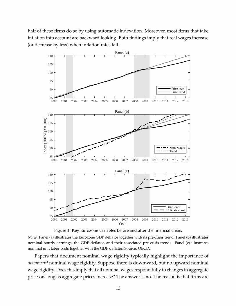
Deflationary pressure. Our paper focuses on recessions during which households’ in-ability to fully insure themselves against increased idiosyncratic risk increases households’desire to save, which puts downward pressure on prices. The top panel of figure 1 showsthe GDP deflator for the Eurozone alongside its pre-crisis trend.22 The figure shows thatthe growth in the price level slowed considerably during the crisis relative to the trend.23

Nominal wage stickiness and inflation. There are many papers that document thatnominal wages are sticky.24 However, what is important for our paper is the question ofto which extent nominal wages adjust to aggregate shocks and, in particular, to changesin the aggregate price level. Druant, Fabiani, Kezdi, Lamo, Martins, and Sabbatini (2009)provide survey evidence for a sample of European firms with a focus on the wages of thefirms’ main occupational groups; these would not change for reasons such as promotion.Another attractive feature of this study is that it explicitly investigates whether nominalwages adjust to inflation or not. In their survey, only 29.7% of Eurozone firms indicate thatthey have an internal policy of taking inflation into account when setting wages, and only

20Our story does not require prices to be procyclical. That is, the channel we identify is also present whenthe precautionary motive only dampens countercyclical behavior.

21Our model has ambiguous predictions for the cyclicality of real wages. If nominal wages respond little tolower inflation and little to lower productivity, then it is possible that the real wage rate increases in responseto a negative shock. In our benchmark model, real wages initially increase following a negative productivityshock, but then start to decrease and fall below previous levels two periods after the shock.

22The pre-crisis trend is defined as the time path the deflators would have followed if inflation beyond theforth quarter of 2007 had been equal to the average inflation rate over the five preceding years.

23Remarkable deflationary pressure is also visible in the US consumer price index (CPI), which droppedby 3.4% during the period from September 2008 to December 2008.

24See, for example, Dickens, Goette, Groshen, Holden, Messina, Schweitzer, Turunen, and Ward (2007),Druant, Fabiani, Kezdi, Lamo, Martins, and Sabbatini (2009), Barattieri, Basu, and Gottschalk (2010), Daly,Hobijn, and Lucking (2012), and Daly and Hobijn (2013).

12

half of these firms do so by using automatic indexation. Moreover, most firms that takeinflation into account are backward looking. Both findings imply that real wages increase(or decrease by less) when inflation rates fall.

2000 2001 2002 2003 2004 2005 2006 2007 2008 2009 2010 2011 2012 201385

90

95

100

105

110Panel (a)

Price levelPrice trend

2000 2001 2002 2003 2004 2005 2006 2007 2008 2009 2010 2011 2012 2013

Inde

x (2

007-

Q3

= 1

00)

85

90

95

100

105

110Panel (b)

Nom. wagesTrend

Year2000 2001 2002 2003 2004 2005 2006 2007 2008 2009 2010 2011 2012 2013

85

90

95

100

105

110Panel (c)

Price levelUnit labor cost

Figure 1: Key Eurozone variables before and after the financial crisis.

Notes. Panel (a) illustrates the Eurozone GDP deflator together with its pre-crisis trend. Panel (b) illustratesnominal hourly earnings, the GDP deflator, and their associated pre-crisis trends. Panel (c) illustratesnominal unit labor costs together with the GDP deflator. Source: OECD.

Papers that document nominal wage rigidity typically highlight the importance ofdownward nominal wage rigidity. Suppose there is downward, but no upward nominalwage rigidity. Does this imply that all nominal wages respond fully to changes in aggregateprices as long as aggregate prices increase? The answer is no. The reason is that firms are

13

heterogeneous and a fraction of firms can still be constrained by the inability to adjustnominal wages downward. In fact, downward nominal wage rigidity is supported bythe empirical finding that the distribution of firms’ nominal wage changes has a largemass-point at zero.25 The fraction of firms that is affected by this constraint would increaseif the aggregate price level increases by less. In fact, Daly, Hobijn, and Lucking (2012)document that the fraction of US workers with a constant nominal wage increased from11.2% in 2007 to 16% in 2011, whereas the fraction of workers facing a reduction in nominalwages was roughly unchanged.26 This indicates that there is upward pressure on realwages when the inflation rate falls, even if it remains positive and nominal wages are onlyrigid downward.

To investigate whether nominal wages followed the slowdown in inflation, the secondpanel of figure 1 displays nominal hourly earnings together with the GDP deflator. Thepanel also shows the realizations of both variables if they would have grown at rates equalto their pre-crisis trends. We find that nominal wages continued to grow at pre-crisis ratesor above, despite a substantial reduction in inflation rates. This means that real wagesincreased relative to trend.27

Real wage costs. The observed increases in real wages are not necessarily due to acombination of low inflation and downward nominal wage rigidity. It is possible that solidreal wage growth reflects an increase in labor productivity, for example, because workersthat are laid off are less productive than those that are not. To shed light on this possibility,we compare the nominal unit wage cost with the price level.28 The results are shown inthe bottom panel of figure 1. The panel shows that nominal unit labor costs have grownfaster than prices since the onset of the crisis, whereas the opposite was true before thecrisis. This indicates that real labor costs increased during the crisis even if one corrects forproductivity.29

25See Barattieri, Basu, and Gottschalk (2010), Dickens, Goette, Groshen, Holden, Messina, Schweitzer,Turunen, and Ward (2007), Daly, Hobijn, and Lucking (2012), and Daly and Hobijn (2013).

26Similarly, at http://nadaesgratis.es/?p=39350, Marcel Jansen documents that from 2008 to 2013 therewas a massive increase in the fraction of Spanish workers with no change in the nominal wage. There issome increase in the fraction of workers with a decrease in the nominal wage, but this increase is smallrelative to the increase in the spike of the histogram at constant nominal wages.

27Similarly, Daly, Hobijn, and Lucking (2012) and Daly and Hobijn (2013) document that real wagesincreased during the recent recession in the US.

28The nominal unit wage cost is defined as the cost of producing one unit of output, i.e., the nominal wagerate divided by labor productivity. The price index used as comparison is the price index used in defininglabor productivity.

29The observation that real unit labor costs are not constant over the business cycle is interesting in itself.If the real wage rate is equal to the marginal product of capital and the marginal product is proportional toaverage labor productivity – properties that hold in several business cycle models – then real unit labor costs

14

These observations are consistent with the hypothesis that the combination of defla-tionary pressure and nominal wage stickiness increased wage costs. In principle, it is stillpossible that nominal wages in the Eurozone did respond fully to prices. However, inthat case, it must be true that the reduction in employment is mainly due to an outflow ofworkers that earn low wages and could produce at low real unit labor cost, since both realwages and real unit labor costs increased. That is, it must be the case that the workers wholeft employment were the ones who had a wage that was low relative to their productivity.This does not seem plausible.

Wages of new and existing relationships. What matters in labor market matching mod-els is the flexibility of wages of newly hired workers. Haefke, Sonntag, and van Rens (2013)argue that wages of new hires respond almost one-to-one to changes in labor productivity.Gertler, Huckfeldt, and Trigari (2014), however, argue that this result reflects changes inthe composition of new hires and that – after correcting for such composition effects –the wages of new hires are not more cyclical than wages of existing employees. Moreimportantly, however, what matters for our paper is whether nominal wages respond tochanges in the price level, and this question is not addressed in either paper. As mentionedabove, Druant, Fabiani, Kezdi, Lamo, Martins, and Sabbatini (2009) find that many firmsdo not adjust wages to inflation. One would think that their results apply to new as well asold matches, since their survey evidence focuses on the firms’ main occupational groups.

3.2 Inability to insure against unemployment risk

An important feature of our model is that workers are poorly insured against unemploy-ment risk. That is, that consumption decreases considerably following a displacement.Using Swedish data, Kolsrud, Landais, Nilsson, and Spinnewijn (2015) document that ex-penditures on consumption goods drop sharply during the first year of an unemploymentspell, after which they settle down at 34% below the pre-displacement level. This sharp fallis remarkable given that Sweden has a quite generous unemployment benefits program.As will be discussed in section 4, one reason is that the amount of assets workers holdat the start of an unemployment spell is low. Another reason is that average borrowingactually decreases during observed unemployment spells.

Using US data Stephens Jr. (2004), Saporta-Eksten (2014), Aguiar and Hurst (2005),Chodorow-Reich and Karabarbounis (2015) provide empirical support for substantialdrops in consumption follow job loss, even when expenditures on durables are not in-

would be constant.

15

cluded.30 Using Canadian survey data, Browning and Crossley (2001) find that workersthat have been unemployed for six months report that their total consumption expenditureslevel during the last month is 14% below consumption in the month before unemployment.

3.3 Savings and idiosyncratic uncertainty

The idea that idiosyncratic uncertainty plays an important role in the savings decisions ofindividuals has a rich history in the economics literature. From a theoretical point of viewKimball (1992) shows that idiosyncratic uncertainty increases savings when the third-orderderivative of the utility function with respect to consumption is positive and/or the agentfaces borrowing constraints. Moreover, idiosyncratic uncertainty regarding unemploymentis more important in recessions which are characterized by a prolonged downturn andan increase in the average duration of unemployment spells. Krueger, Cramer, and Cho(2014) document that during the recent recession the number of long-term unemployedincreased in Canada, France, Italy, Sweden, the UK, and the US. They only case in whichthey found a decrease is Germany. The results are particularly striking for the US. Duringthe recent recession, the amount of workers who were out of work for more than half ayear relative to all unemployed workers reached a peak of 45%, whereas the highest peakobserved in previous recessions was about 25%.

Several papers have provided empirical support for the hypothesis that increases inidiosyncratic uncertainty increases savings. Using 1992-98 data from the British HouseholdPanel Survey (BHPS), Benito (2004) finds that an individual whose level of idiosyncraticuncertainty would move from the bottom to the top of the cross-sectional distributionreduces consumption by 11%. An interesting aspect of this study is that the result holdsboth for a measure of idiosyncratic uncertainty based on an individuals’ own perceptionsas well as on an econometric specification.31 Further empirical evidence for this relation-ship during the recent downturn can be found in Alan, Crossley, and Low (2012). They

30Using the four 1992-1996 waves of the Health and Retirement Study (HRS), Stephens Jr. (2004) finds thatannual food consumption is 16% lower when a worker reports that he is no longer working for the employerof the previous wave either because of a layoff, business closure, or business relocation, that is, the workerwas displaced between two waves. Similar results are found using the Panel Study of Income Dynamics(PSID). Using the 1999-2009 biannual waves of the PSID, Saporta-Eksten (2014) finds that job loss leads to adrop in total consumption of 17%. About half of this loss occurs before job loss and the other half aroundjob loss. The drop before job loss suggests that either the worker anticipated the layoff or labor income wasalready under pressure. Moreover, this drop in consumption is very persistent and is only slightly less than17% six years after displacement. Using data for food and services, Chodorow-Reich and Karabarbounis(2015) find that the consumption level of workers that are unemployed for a full year is 21% below theconsumption level of employed workers. Using scanner data for food consumption, Aguiar and Hurst (2005)report a drop of 19%.

31Although the sign is correct, the results based on individuals’ own perceptions are not significant.

16

argue that the observed sharp rise in the savings ratio of the UK private sector is drivenby increases in uncertainty, rather than other explanations such as tightening of creditstandards. In line with the mechanism emphasized in this paper, Carroll (1992) arguesthat employment uncertainty is especially important because unemployment spells are thereason for the most drastic fluctuations in household income. In addition, Carroll (1992)provides empirical evidence to support the view that the fear of unemployment leads toan increased desire to save even when controlling for expected income growth.

4 Calibration

This section starts with a discussion of the parameter values that play a key role ingenerating the results, followed by a discussion of the remaining and less crucial parametervalues. The model period is one quarter. Targets are constructed using Eurozone data from1980 to 2012.32 We focus on the Eurozone for two reasons. First, our empirical results forthe Eurozone indicate that inflation slowed down during the crisis and nominal unit wagecosts did not.33 Second, many economists have warned of the risks of a deflationary spiralin the Eurozone.34

Key parameter values. Regarding the choice of key parameter values, our strategy is toshow that our main results can be generated with conservative choices. For example, weset the coefficient of relative risk aversion equal to 2. Even though risk aversion is not thathigh, the differences between our heterogeneous-agent model and the representative-agentversion are substantial.

The incidence and duration of unemployment spells are obviously important. Theprobability of job destruction, δ, and the parameter characterizing efficiency in the match-ing market, ψ, are chosen to ensure that the unemployment rate and the expected durationof an unemployment spell in the economy without aggregate risk match their observedcounterparts, which are equal to 10.7% and 3.57 quarters, respectively.35 These numbers

32Average unemployment duration data are based on all of Europe, since no Eurozone data is availablefor this time period. Details about data sources are given in appendix A.

33We found that this is not the case for the US even though – similar to Eurozone developments – realwages did increase sharply during the crisis.

34According to the May 2014 survey of the Centre for Macroeconomics, half of the macroeconomists inthe panel thought that there was a significant risk of sustained negative inflation in the coming two years.Details can be found at http://cfmsurvey.org/surveys/euro-area-deflation-and-risk-uk-economy-may-2014.For our story, inflation does not have to be negative. It is sufficient if deflationary pressure lowers inflation,which increases real wage costs when nominal wages are sticky.

35Finding the right parameter values requires solving the model numerous times, which is very computerintensive for the model with aggregate uncertainty. For that reason, we calibrate these parameters by

17

suggest a 3.36% quarterly job separation rate and a value for ψ equal to 0.574, implying aquarterly matching probability of 28%.

Unemployment insurance regimes vary a lot across countries in Europe. Esser, Ferrarini,Nelson, Palme, and Sjoberg (2013) report that net replacement rates for insured workersvary from 20% in Malta to just above 90% in Portugal. Most countries have net replacementrates between 50% and 70% with an average duration of around one year. Coverage ratiosvary from about 50% in Italy to 100% in Finland, Ireland, and Greece. Net replacementrates for workers that are not covered are much lower. In most countries, these are less than40%. In the model, unemployment benefits are set equal to 50% and – for computationalconvenience – are assumed to last for the entire duration of the unemployment spell.A replacement rate of 50% is possibly a bit less than the average observed, but this iscompensated for by the longer duration of unemployment benefits in the model.

The inability to fully insure against unemployment risk plays a key role. It is, therefore,important that the model generates a realistic drop in consumption during an unem-ployment spell. While data for the Eurozone is unavailable for this purpose, Kolsrud,Landais, Nilsson, and Spinnewijn (2015) provide evidence for Sweden. They report thatconsumption drops on average by 34% during the first year of an unemployment spell.A key parameter to target this number is the scale parameter, χ, which characterizes theliquidity benefits of money.36 This parameter affects the average level of financial assetsheld and, thus, the ability of agents to insure against unemployment spells. The literaturealso provides some evidence on pre-displacement wealth levels. Gruber (2001) providesevidence for the US. In section 5, we will show that our calibration is conservative. That is,we generate the targeted consumption drop without making agents unrealistically poor.

The main focus of this paper is on the interaction between sticky nominal wages andthe deflationary pressure arising from uncertain job prospects. Consequently, a key role isplayed by ωP, the parameter that indicates how responsive nominal wages are to changesin the price level. Our benchmark value for ωP is equal to 0.7, which means that a 1%increase in the price level leads to an 0.7% increase in nominal wages. As mentionedbefore, Druant, Fabiani, Kezdi, Lamo, Martins, and Sabbatini (2009) report that only 6% ofEuropean firms adjust wages (of their main occupational groups) more than once a year toinflation and only 50% do so once a year.37

matching the targets in the model without aggregate uncertainty. The corresponding statistics in the modelwith aggregate uncertainty are somewhat different; the average unemployment rate is equal to 11.7% andthe average duration is equal to 4.03 quarters.

36Its calibrated value is equal to 4.00e− 5.37Moreover, even if firms adjust for inflation they typically do so using backward looking measures of

inflation, which reduces the responsiveness to changes in inflationary pressure.

18

Finally, the curvature parameter in the utility component for liquidity services, ζ, playsan important role, because it directly affects the impact of changes in future job securityon the demand for the liquid asset. With more curvature, the demand for the liquidasset is less sensitive and increased concerns about future job prospects will generate lessdeflationary pressure. We follow Lucas (2000), and target a money demand elasticity withrespect to the nominal interest rate equal to −0.5. The resulting value of ζ is equal to 2.38

Other parameter values. Based on the empirical estimates in Petrongolo and Pissarides(2001), the elasticity of the job finding rate with respect to tightness, η, is set equal to 0.5.The average share of the surplus received by workers, ω0, and the elasticity of the wagerate with respect to changes in aggregate productivity, ωz, are set such that the standarddeviation of employment relative to the standard deviation of output are in line with theirempirical counterpart.39

In our model, the presence of idiosyncratic risk lowers average real rates of return. Thismotivates us to set the discount factor, β, to 0.985, which is slightly below its usual value of0.99.40 The two values for zt are 0.978 and 1.023 and the probability of switching is equalto 0.025.41 Finally, money supply, M, is chosen such that the average price level, P, is equalto 1.

Parameters values in the representative-agent model. We will compare the resultsof our model with those generated by the corresponding representative-agent econ-omy. Parameter values in the representative-agent model are identical to those in the

38The first-order condition for a bond with a risk-free nominal interest rate is given by

1 = β (1 + Rt) βEt

[(ci,t+1

ci,t

)−γ

Pt/Pt+1

].

Using (1 + Rt)−1 ≈ 1− Rt, we get

ln (Mi,t+1/Pt) ≈ −ζ−1 ln Rt + ζ−1 (ln χ + γ ln ci,t) .

The other key parameter in money demand functions is the elasticity with respect to income, which capturesthe volume of transactions. Our transactions variable is consumption and the elasticity of money demandwith respect to consumption is equal to γ/ζ, which equals 1 for our choices for the coefficient of relative riskaversion, γ, and ζ.

39In the benchmark economy, ω0 = 0.97 and ωz = 0.3. Without our deflationary mechanism, one wouldhave to choose a higher value for ω0 and/or a lower value for ωz to generate the same amount of volatilityin employment as pointed out in Hagedorn and Manovskii (2008).

40At this relatively high 6% annual discount rate, the average real rate of return is already quite low,namely 0.72% on an annual basis in the economy with aggregate uncertainty.

41These values are chosen to ensure that E[ln zt] = 0, Et[ln zt+1] = 0.95 ln zt, and Et[(ln zt+1 −Et[ln zt+1])

2] = 0.0072.

19

heterogeneous-agent model, except for β. Using the model without aggregate shocks,we choose the value of β for the representative-agent model such that the MRS in therepresentative-agent model is equal to the MRS for the agents holding equity in theheterogeneous-agent model.42 Without this adjustment, the agent in the representative-agent economy would have a more shortsighted investment horizon and average employ-ment would be lower.

5 Agents’ consumption, investment and portfolio decisions

In section 5.1, we describe key aspects of the behavior of individual consumption, andin particular its behavior during an unemployment spell. In section 5.2, we focus on theindividuals’ investment portfolio decisions.

5.1 Post-displacement consumption

In this section, we first discuss the reduction of individual consumption following dis-placement, and then turn to the factors that are behind the substantial drop generated bythe model.

Magnitude of the post-displacement drop in consumption. Figure 2 displays the aver-age post-displacement change in consumption. The model’s parameters are calibratedsuch that the one-year drop equals its empirical equivalent, that is 34%. Although nottargeted, the model predicts a proportional decrease over the first year similar to what isobserved in the data.43 However, whereas the data indicate that the fall in consumptionsettles down after one year, the model suggests that this happens first after two years.Nevertheless, figure 3 documents the distribution of the duration of unemployment andshows that most unemployment spells do not exceed one year.44

There are several reasons why the drop in consumption is of such a nontrivial magni-tude. One reason is, of course, that unemployment benefits are only half as big as laborincome. But a key factor affecting the magnitude of the drop is the average level of wealthat the beginning of an unemployment spell. Using US data, Gruber (2001) finds that themedian agent holds enough gross financial assets to cover 73% of the average net-income

42Notice that the expected intertemporal marginal rate of substitution, βEt

[(ci,t+1/ci,t)

−γ], is constant

and the same for all agents holding equity in the model without aggregate shocks.43See Kolsrud, Landais, Nilsson, and Spinnewijn (2015).4481% of all unemployment spells that start in an expansion last at most four quarters. The corresponding

number for recessions is 61%.

20

loss during an unemployment spell. Moreover, in terms of net financial assets, the median

−1 0 1 2 3 4 5 6 7 8 9 10

−50

−45

−40

−35

−30

−25

−20

−15

−10

−5

0

Duration of unemployment spell (quarters)

Per

c. c

hang

e

Cond. on expansionCond. on recession

Figure 2: Evolution of consumption drop over the unemployment spell.

Notes. The black line illustrates the average path of consumption of an individual that becomes unemployedin period 1, conditional on being in an expansion at the time of displacement. The grey line illustrates theequivalent path conditional on being in a recession.

0 2 4 6 8 10 12 14 16 18 200

0.05

0.1

0.15

0.2

0.25

0.3

0.35

0.4

Duration of unemployment spell (quarters)

Freq

uenc

y

Cond. on expansionCond. on recession

Figure 3: Distribution of the unemployed.

Notes. The black bars measure the fraction of unemployed at various durations conditional on being in anexpansion at the time of displacement. The grey bars provide the corresponding measure conditional onbeing in a recession.

21

agent does not even have enough to cover 10% of the average net-income loss.45 Onewould expect that agents accumulate less savings in Europe where unemployment benefitsare higher.46 In our model, the median agent’s asset holdings are equal to 54% of theaverage net-income loss during unemployment spells. This is true for both gross and netasset holdings, since there is no debt in our model. Thus, relative to these observed levels,the median agent is less wealthy in terms of gross financial assets, but a lot wealthier interms of net financial assets.

Figure 4 displays the complete cumulative distribution function of the value of assetsat the beginning of an unemployment spell relative to the average net-income loss. Agentsin the bottom of the wealth distribution are substantially richer than their real worldcounterparts, even if we focus on gross assets. For example, Gruber (2001) documentsthat 38% of all workers do not have enough assets to cover 25% of the average net-incomeloss. In our model, the corresponding fraction is only 7%. Thus, it is not the case that werely on unrealistically low wealth levels to generate the sizeable fall in post-displacementconsumption observed in the data.

The question arises why infinitely-lived agents do not build a wealth buffer thatinsulates them better against this consumption volatility, as is the case in the model ofKrusell and Smith (1998).47 The key parameter used to match the observed decline inpost-displacement consumption is the scaling coefficient affecting the utility of money, χ.Choosing a low value for χ to match the observed decline in consumption implies thatmoney holdings – one of the two wealth components – are, on average, lower. The otherwealth component is the value of equity holdings, Jtqi,t. Elevated uncertainty about futureindividual consumption increases the expected value of an agent’s MRS, which wouldincrease the price of equity, Jt. As a consequence, the number of new firms as well asthe total number of shares outstanding would therefore rise. However, there are severalreasons why this component of wealth is not very large in our model. First, the equityprice, Jt, cannot increase by too much, because the presence of a liquidasset with a positive

45Gross financial assets would be the relevant measure if debt can be rolled over during an unemploymentspell. Net financial assets would be the relevant measure if that is not the case. Kolsrud, Landais, Nilsson,and Spinnewijn (2015) find that average debt decreases during unemployment spells, which means that theobserved gross measure clearly overestimates the amount of funds agents have to cover income losses.

46In contrast to Gruber (2001), Kolsrud, Landais, Nilsson, and Spinnewijn (2015) do not provide pre-displacement wealth levels as a function of expected earnings losses. But some information is available. Inparticular, using an average unemployment spell duration of 4 months, the median Swedish agent’s levelof gross financial assets is equal to roughly 13% of average net-income loss. In our model, calibrated to anaverage level of European unemployment benefits, net income drops by more (by half as opposed to onethird in Sweden), but agents that become unemployed are wealthier.

47For the model of Krusell and Smith (1998), solved in Den Haan and Rendahl (2010) using a 15%unemployment replacement rate, the average post-displacement consumption drop is 5% after one year,whereas we find a 34% drop with a 50% unemployment replacement rate.

22

transactions benefit puts a lower bound on the average real return on equity. Moreover,the nonlinearity of the matching function dampens the impact of an increase in equityprices on the creation of new firms. Lastly, the equity price depends positively on theaverage share of output going to firm owners, 1−ω0. To generate sufficient volatility inemployment we chose a relatively high value for ω0, which reduces the value of Jt.48 Forall these reasons, agents in our model do not build up large buffers of real money balancesor equity to insure themselves against the large declines in consumption upon and duringunemployment.

0 0.1 0.2 0.3 0.4 0.5 0.6 0.7 0.8 0.9 10

0.1

0.2

0.3

0.4

0.5

0.6

0.7

0.8

0.9

1

Value of assets relative to average net−income loss

Cum

ulat

ive

dist

ribut

ion

Figure 4: Financial assets at the beginning of an unemployment spell.

Another aspect affecting consumption during unemployment is the ability to borrow.In our model, agents cannot go short in any asset, and they would presumably holdless financial assets if they had the option to borrow. Kolsrud, Landais, Nilsson, andSpinnewijn (2015) report, however, that the amount of consumption that is financed out ofan increase in debt actually decreases following a displacement. More importantly, we thinkthat the key feature to capture is the level of the drop in consumption upon and during

48A small modification of the model would decrease the value of output going to workers and have onlymarginal effects on the main mechanism. In particular, suppose that output is increased from zt to (1 + Λ)ztwith Λ > 0. Also, suppose that operating a firm depends on using an additional factor, say land. This factoris owned by another agent for whom this is the only source of income. If bargaining is such that this factorreceives Λzt each period, then our numerical results are exactly the same except that total GDP is now equalto (1 + Λ)ztqt. This modification increases output by Λ% , but has a much bigger impact on the net presentvalue of the additional non-labor income stream. Consequently, with a small value for Λ the model wouldbe more realistic in terms of having more wealthy agents while leaving the other properties of the modellargely unchanged.

23

unemployment, and not whether this is accomplished by limited borrowing or by someborrowing combined with a lower level of financial assets.

State dependence of consumption drop. Figure 5 presents a scatter plot of the reductionin consumption (y-axis) and beginning-of-period cash on hand (x-axis), where both aremeasured in the period when the agent becomes unemployed.49 There are two distinctpatterns, one for expansions and one for recessions.50

0 0.5 1 1.5 2−40

−35

−30

−25

−20

−15

−10

−5

0

Real cash on hand

Per

c. c

hang

e

MeanMean

ExpansionRecession

Figure 5: Consumption drop upon becoming unemployed.

Consistent with figure 2, figure 5 documents that the drop in consumption is, on average,much more severe if the unemployment spell initiates in a recession. The figure alsounderscores the non-trivial role played by the agents’ wealth levels. In particular, duringrecessions the decline in consumption varies from 18.9% for the richest agent to 35.1% forthe poorest. This range increases during an expansion: The richest agent faces a modestdrop of 8.8%, whereas the poorest agent can expect to see consumption fall by 33.9%. Thelatter is only slightly below the equivalent number in a recession.

There are several reasons why consumption falls by more during recessions. First, jobfinding rates are on average lower in recessions than in expansions. As a consequence,

49Cash on hand is equal to the sum of non-asset income (here unemployment benefits), money balances,dividends, and the value of equity holdings.

50The level of employment is also important for the observed decline in consumption, which explains thescatter of observations. In particular, the fall in the level of consumption is smaller at the beginning of anexpansion and larger at the beginning of a recession. The reason is that expected investment returns arehigher (lower) at the beginning of the expansion (recession), which would put upward (downward) pressureon consumption when the income effect dominates the substitution effect.

24

agents anticipate longer unemployment spells and will, for a given amount of cash onhand, therefore reduce consumption more sharply. A second factor that affects agents’reduced consumption is the amount of cash on hand they hold. Because the price of equitydeclines in recessions, so does the agents’ cash on hand. Indeed, the average value of cashon hand held by a newly unemployed agent is equal to 1.26 in a recession compared to1.68 in an expansion.

In reality, a typical worker may not face such a large decline in the value of their equityposition when the economy enters a recession. After all, quite a few workers do not ownequity at all. We think, however, that the cyclicality of post-displacement consumptionbehavior that is driven by the cyclicality of equity prices, capture real world phenomena.First, although not all workers hold equity, many hold assets such as housing that alsohave volatile and cyclical prices. Second, unemployed workers may receive handouts, andor loans, from affluent family members, friends, or financial intermediaries whose abilityand willingness may be affected by the value of their assets, which is likely to be cyclical.

5.2 Investment decisions

A key aspect of our heterogeneous-agent model is that money demand increases duringrecessions, whereas it decreases in the representative-agent version. In this section, weshed light on this difference. In particular, we first discuss how portfolio shares vary withagents’ wealth levels, employment status, and the business cycle. We then turn to thebehavior of money demand along the same dimensions.

Portfolio composition and cash-on-hand levels. Figure 6 presents a scatter plot of theliquid asset’s share in the agents’ investment portfolios (y-axis) and the beginning-of-period cash-on-hand levels (x-axis). Although the pattern is somewhat intricate, the figurecan be characterized reasonably well as follows. First, the fraction invested in money ishigher at lower cash-on-hand levels. Second, conditional on the cash-on-hand level, thisfraction also increases when an agent becomes unemployed. Third, conditional on the cash-on-hand level and employment status, this fraction increases when the economy enters arecession. These three properties imply that the portfolio share invested in money increasesduring a recession. Without large enough increases in money portfolio shares, aggregatedemand for money would decrease during recessions, like it does in the representative-agent model. This is because the total amount of funds carried over into the next perioddecreases during recessions, which in turn implies that the value of agents’ portfolios islower.

25

0 0.5 1 1.5 2 2.5 30

0.1

0.2

0.3

0.4

0.5

0.6

0.7

0.8

0.9

1

Real cash on hand

Shar

e

Employed in expansionUnemployed in expansionEmployed in recessionUnemployed in recession

Figure 6: Portfolio shares in liquid asset.

Notes. This figure displays the fraction of financial assets invested in the liquid asset as a function ofbeginning-of-period cash on hand for workers of the indicated employment status and for both outcomes ofaggregate productivity

Which forces explain the observed patterns? The first is that the transaction benefits ofmoney are subject to diminishing returns. As a consequence, agents whose total demandfor financial assets is high tend to invest a smaller fraction in money. This explains whythe fraction invested in money is generally lower for agents with higher cash-on-handlevels. The second driving force is that money is less risky than equity. Therefore, agentswhose total demand for financial assets is high relative to their non-asset income invest alarger fraction in money. For a given cash-on-hand level, this explains why the fractioninvested in money increases when a worker becomes unemployed, and why the fractionincreases when the economy enters a recession.51 The observed patterns are intricatebecause these two features push the money portfolio share in different directions and theoutcome depends on the relative strengths of each force.

Money demand and cash on hand. Figure 7 presents a scatter plot of the demand forreal money balances (y-axis) and beginning-of-period cash-on-hand levels (x-axis). Thereare four distinct patterns depending on the stance of the business cycle (expansion or

51Notice that for a given cash-on-hand level unemployed agents are more asset rich than employed agents,and therefore demand more money. The Euler equation for money, equation (3), implies a monotone positiverelationship between the level of money demand and the level of consumption when there is no aggregateuncertainty, because the expected marginal rate of substitution is constant in that case. This implies that theunemployed hold a lower amount of money balances.

26

recession) and the agent’s employment status. As discussed above, almost all unemployedworkers hold larger shares of their portfolio in the liquid asset than employed workers, andboth types of workers typically hold a larger share in the liquid asset during recessions thanduring expansions. Figure 7 shows that both properties are also true when we considerthe amount of real money balances as opposed to its share in the portfolio.52 The figurealso illustrates that – everything else equal – the demand for real money balances increaseswith beginning-of-period cash on hand.

0 0.5 1 1.5 2 2.5 30

0.1

0.2

0.3

0.4

0.5

0.6

0.7

0.8

0.9

Real cash on hand

Mon

ey d

eman

d

Employed in expansionUnemployed in expansionEmployed in recessionUnemployed in recession

Figure 7: Money demand (real).

Notes. This figure displays the amount invested in the liquid asset as a function of beginning-of-period cashon hand for workers of the indicated employment status and for both outcomes of aggregate productivity

A key result of this paper is that the interaction between sticky nominal wages andthe inability to insure against unemployment risk deepens recessions. An integral partof the mechanism underlying this result is the upward pressure on money demand thatemerges when job prospects worsen. When the economy enters a recession, aggregatemoney demand is pushed in opposite directions by different factors. In particular, duringrecessions aggregate cash on hand falls, since equity prices fall. This reduces demandfor all assets, including real money balances. Because of incomplete markets, however,there are two further reasons that explain why aggregate demand for money increasesin our economy. As documented in figure 7, for given cash-on-hand levels, all agentsdemand more money during recessions. Lastly, unemployed agents demand more money

52Whereas the observations are typically true when the share invested in the liquid asset is considered, theobservations are always true when the level of money demand is considered.

27

than employed agents, and there are more unemployed agents in the economy duringrecessions. The last two effects dominate the first, and aggregate money demand increasesduring recessions. This result stands in sharp contrast with the representative-agentversion of our economy, in which aggregate money demand unambiguously decreasesduring recessions.

To see that this is a remarkable result, envisage a partial equilibrium version of ourmodel in which the price level, wages, and the equity price are all constant, and there isno short-sale constraint. Markets are still incomplete because the agents cannot insurefully against unemployment risk. Now consider a temporary decrease in the job findingprobability. Could this lead to an increase in the demand for real money balances? Theanswer is no. In this economy, demand for real money balances, Mi,t+1/Pt, and consump-tion, ci,t always move in the same direction. In particular, when agents lower consumptionin response to a decrease in the job finding probability, money demand will decrease aswell. The reason is the following. The Euler equation for equity in (4) – which now holdswith equality – implies that the individual MRS is unaffected by the increase in risk.53 TheEuler equation for money in (3) then directly implies that ci,t and Mi,t+1/Pt move in thesame direction. By contrast, in our model – in which prices adjust to clear markets and theshort-sale constraint is binding for some agents – aggregate money demand and aggregateconsumption move in opposite directions.

Financial assets during unemployment spells. Consumers dampen the drop in con-sumption following displacement by selling financial assets. Figures 8 and 9 documentwhat this means for equity and money holdings, respectively. Although the total amountof financial assets, and the amount invested in equity, sharply decrease, the amount heldin the liquid asset actually increases during the first two periods of an unemployment spell.The loss of wage income means that workers’ cash-on-hand levels drop when they becomeunemployed. This reduces the demand for real money balances. However, and as dis-cussed above, the unemployed actually hold more money for a given level of cash on hand.Figure 9 documents that the last effect dominates in the beginning of an unemploymentspell.

53In this case, equation (4) can be rearranged as

Jt = βEt

[(ci,t+1

ci,t

)−γ](D + (1− δ)Jt+1) ,

which implies that the individual MRS, βEt

[(ci,t+1/ci,t)

−γ], is pinned down by aggregate prices only, and

is therefore unaffected by risk.

28

−1 0 1 2 3 4 5 6 7 80

0.1

0.2

0.3

0.4

0.5

0.6

0.7

0.8

0.9

1

Unemployment duration (quarters)

Equ

ity h

oldi

ngs

Cond. on expansionCond. on recession

Figure 8: Post displacement equity holdings.

Notes. The black line illustrates the average path for equity holdings of an individual that becomes unem-ployed in period 1, conditional on being in an expansion at the time of displacement. The grey line illustratesthe equivalent path conditional being in a recession.

−1 0 1 2 3 4 5 6 7 80

0.1

0.2

0.3

0.4

0.5

0.6

Unemployment duration (quarters)

Mon

ey h

oldi

ngs

Cond. on expansionCond. on recession

Figure 9: Post displacement money holdings.

Notes. The black line illustrates the average path for money holdings of an individual that becomes unem-ployed in period 1, conditional on being in an expansion at the time of displacement. The grey line illustratesthe equivalent path conditional on being in a recession.

29

6 Economic aggregates over the business cycle

In the previous section, we showed that the inability of agents to insure against unem-ployment risk means that workers face a sharp drop in consumption when they becomeunemployed. We also discussed how imperfect insurance affects money demand in waysthat are not present in an economy with complete markets. In this section, we discuss whatthis implies for aggregate activity. In particular, we document and explain why the inter-actions between sticky nominal wages, gloomy outlooks regarding future employmentprospects, and the inability to insure against unemployment risk can deepen recessions.We first compare the business cycle properties of the benchmark economy with imperfectrisk sharing and sticky nominal wages, i.e. ωP < 1, to those of an economy with full risksharing. Subsequently, we discuss the same comparison when nominal wages are notsticky, i.e., ωP = 1.

6.1 The role of imperfect insurance when nominal wages are sticky

Figure 10 shows the impulse response functions (IRFs) of key aggregate variables toa negative productivity shock for our benchmark economy and for the correspondingrepresentative-agent economy.54 The two graphs in the top row of the figure display theresponses for output and employment. These two graphs document that the economy withincomplete risk sharing faces a much deeper recession than the economy with completerisk sharing. In particular, output drops by 7.2% in the heterogeneous-agent economy andby only 4.3% in the representative-agent economy.

The key aspect in understanding this large difference is the behavior of the price level.In the representative-agent economy, the reduction in real activity decreases the demandfor money and increases the price level. In our benchmark calibration wages are sticky(ωP = 0.7), and a 1% increase in the price level leads to a 0.7% increase in nominal wagesand therefore a 0.3% decrease in real wages. Thus, the direct effect of the reduction ofproductivity, zt, on profits is counteracted, because nominal wages do not fully respondto the associated increase in the price level. That is, our starting point is an economy inwhich the sluggish response of nominal wages to changes in prices actually dampens theeconomic downturn.

54In our benchmark calibration, productivity takes on only two values. The IRFs are calculated as follows.The starting point is period s, when productivity takes on its “expansion” value and employment is equal toits mean value conditional on being in an expansion. We then calculate the following two time paths foreach variable. The “no-shock” time path is the expected time path from this point onward. The “shock” timepath is the expected time path when the productivity switches to the low value in period s + 1. The IRF is thedifference between these two time paths.

30

0 10 20 30 40 50−0.08

−0.07

−0.06

−0.05

−0.04

−0.03

−0.02

−0.01

0

Log

devi

atio

nOutput and productivity (dashed line)

Incompl. marketsCompl. markets

0 10 20 30 40 50−4

−3.5

−3

−2.5

−2

−1.5

−1

−0.5

0

0.5

Ppt

. dev

iatio

n

Employment

0 10 20 30 40 50−0.7

−0.6

−0.5

−0.4

−0.3

−0.2

−0.1

0

Log

devi

atio

n

Time (quarters)

Asset prices

0 10 20 30 40 50−0.15

−0.1

−0.05

0

0.05

0.1

Time (quarters)

Log

devi

atio

n

Price level

Figure 10: Impulse responses with sticky nominal wages

Notes. These graphs illustrate the difference between the expected time path when the economy is in anexpansion in period 0 and the expected time path conditional on being in a recession in period 1. ωP = 0.7,i.e., nominal wages increases with 0.7% when prices increase with 1%.

By contrast, the price level falls in the heterogeneous-agent economy. This fall is causedby an increase in the aggregate demand for the safer asset, i.e., money. To understandthis different outcome, consider again figure 7, which illustrates the relationship betweenthe demand for money as a function of beginning-of-period cash-on-hand levels duringexpansions and recessions, for both employed and unemployed agents. The reduction inreal activity lowers cash-on-hand levels which reduces the demand for money by bothemployed and unemployed agents. The drop in cash-on-hand levels is substantial becausethe value of equity declines sharply. Nevertheless, aggregate money demand increases. As

31

previously discussed, both employed and unemployed agents hold more money duringrecessions for the same cash-on-hand level. In addition, there are more unemployed agentsduring recessions, and unemployed agents have larger money holdings than employed atthe same level of cash on hand.

Whereas sticky nominal wages reduce the depth of recessions in the representative-agent economy, they worsen recessions in the heterogeneous-agent economy. This is aquantitatively important effect, because a reduction in the price level (for any reason)starts a self-reinforcing process that deepens recessions. In particular, the reduction in theprice level puts upward pressure on real wages, which reduces profits. The fall in profitsreduces investment in new jobs, which in turn reduces employment.55 Since this reductionin employment is persistent, employment prospects worsen. With elevated risk there is afurther increase in the demand for money, which in turn puts additional upward pressureon the price level, and so on. The impulse responses show that this mechanism is powerfulenough to completely overturn the dampening effect that sticky nominal wages have in aneconomy with complete risk sharing.

Although this is a powerful mechanism, there is a counterforce. In particular, a higherunemployment rate increases the probability that a firm finds a worker, even at a givenlevel of investment. For the results reported here, this counterforce is strong enough toensure stability. For some parameter values, the fluctuations could very well become solarge that no non-explosive solution exists.56

6.2 Role of imperfect insurance when nominal wages are not sticky

In this section, we discuss business cycle properties when changes in the price level leavereal wages unaffected, that is, ωP = 1. Figure 11 plots the IRFs for the heterogeneous-agenteconomy and the IRFs for the corresponding representative-agent economy. There areseveral similarities with our benchmark results, but also one essential difference. We startwith the similarities.

55The negative productivity shock still has a direct negative effect on real wages. Which effect is strongerdepends on parameter values. In our benchmark economy, the impulse response function of real wages ispositive for the first two years and then turns negative.

56In particular, changes in parameter values that substantially enhance the deflationary mechanism makeit computationally challenging, or even impossible, to find an accurate solution. This does not prove thata stationary solution does not exist, but it would be consistent with this hypothesis. If such a solutionwould exist, however, it is likely to have complex nonlinear features. This result is in contrast to standardperturbation methods which impose that aggregate shocks of any size will not destabilize the economyas long as arbitrarily small shocks do not. For example, the technique developed in Reiter (2009) to solvemodels with heterogeneous agents relies on a perturbation solution for changes in the aggregate shock,which implies that the solution is imposed to be stable – for shocks of any size – as long as the Blanchard-Kahnconditions are satisfied. Our experience suggests that this may impose stability where there is none.

32

0 10 20 30 40 50−0.07

−0.06

−0.05

−0.04

−0.03

−0.02

−0.01

0

Log

devi

atio

nOutput and productivity (dashed line)

Incompl. marketsCompl. markets

0 10 20 30 40 50−3.5

−3

−2.5

−2

−1.5

−1

−0.5

0

0.5

Ppt

. dev

iatio

n

Employment

0 10 20 30 40 50−0.45

−0.4

−0.35

−0.3

−0.25

−0.2

−0.15

−0.1

−0.05

0

Log

devi

atio

n

Time (quarters)

Asset prices

0 10 20 30 40 50−0.1

−0.05

0

0.05

0.1

0.15

Time (quarters)

Log

devi

atio

n

Price level

Figure 11: Impulse responses with flexible nominal wages

Notes. These graphs illustrate the difference between the expected time path when the economy is in anexpansion in period 0 and the expected time path conditional on being in a recession in period 1. ωP = 1,that is, nominal wages respond 1-for-1 to price changes.

A negative productivity shock still has a direct negative effect on profits, which leadsto a reduced demand for equity (firm ownership), which in turn means that fewer jobs arecreated. Also, increased concerns about employment prospects still induce agents in theheterogeneous-agents economy to increase their demand for money holdings, which againis strong enough to push the price level down, while it increases in the representative-agenteconomy.

There is also a striking difference. In the economy with flexible nominal wages, reces-sions are less severe when agents cannot insure themselves against unemployment risk.

33

The reason is the following. Increased uncertainty, alongside with an expected reductionin individual consumption, increase the expected value of the marginal rate of substitution.This affects the first-order condition of the liquid asset as well as the first-order condition ofthe productive investment, at least if each agent’s future revenues are discounted by theirown individual MRS. Since wages are flexible, the associated rise in the price level bears noconsequence on the return on equity, and the chain of events underlying the deflationaryspiral breaks down.

Thus, if the rise in precautionary savings is partially used as productive investments,then this would dampen the reduction in the demand for equity induced by the directnegative effect of the productivity shock on profits. The IRFs document that this is indeedthe case when nominal wages respond one-for-one to changes in the price level. Themagnitude of the dampening effect is nontrivial. Whereas the biggest drop in employmentis 3.3ppt in the representative-agent economy, it is equal to 2.7ppt in the heterogeneous-agent economy. These results make clear that a researcher would bias the model predictionsif this dampening aspect of precautionary savings is not allowed to operate, for example,because there is communal firm ownership.57

In our benchmark economy, we allow this channel to operate, but the effect is dominatedby the interaction between sticky nominal wages and uninsurable unemployment risk.Increased uncertainty may increase the demand for equity, but it will also increase thedemand for money. Increased money demand depresses the price level, which, providedthat nominal wages are somewhat sticky, increases real wages. The rise in real wagesreduces profits, which in turn lowers the demand for equity. This channel dominates anypositive effect that precautionary savings may have on the demand for equity.

Robustness of the dampening effect. In all cases considered, we find that recessionsare less severe in the heterogeneous-agent economy than in the representative-agenteconomy if nominal wages respond one-for-one to change in the price level. That is,this dampening effect is very robust. During the nineties, several papers argued that anincrease in idiosyncratic risk could lead to a reduction in the demand for a risky asset wheninvestors can save through both a risky and a risk-free asset even though it would increasetotal savings. This effect is referred to as temperance.58 We find that this result is quitefragile for several reasons.

The first is that it is a partial equilibrium result. In general equilibrium prices adjust.This is important. Suppose that the economy as a whole can increase savings through the

57See footnote 6 for a list of papers following this approach.58See Kimball (1990), Kimball (1992), Gollier and Pratt (1996), and Elmendorf and Kimball (2000).

34

risky investment, but not through the risk-free investment. Then the relative price of therisk-free asset would increase making the riskier asset more attractive. This plays a role inour economy, because the only way the economy as a whole can do something now to havemore goods in the future is by investing more in the productive asset, that is, in the riskyasset. There are several other features, typically present in macroeconomic models, thatmake temperance less likely. One is that the temperance result relies on idiosyncratic riskto be sufficiently independent of investment risk. In macroeconomic models, that is notthe case. The amount of idiosyncratic risk depends on the level of the wage rate.59 But thelevel of the wage rate is often correlated with the return of the risky asset, since both areaffected by the same shocks.60 In appendix D, we show that this feature alone can overturnthe temperance result even in a partial equilibrium setting. Another feature that worksagainst the temperance result is the short-sale constraint on equity, which directly preventsa reduction in the demand for equity, at least for some agents. In our model, diminishingreturns on the transactions aspect of money also work against temperance. This makesincreased investment in the risk-free asset less attractive relative to a framework in whichthe return remains fixed. In appendix D, we show that this can overturn the temperanceresult by itself even if the transactions component is very small and there is little convexityin the marginal return on money balances. Finally, in our model, money is not nearly asrisky as equity, but it is also not completely risk-free.

It may be the case that temperance can be generated in models with different utilityfunctions, for example, if the utility function is such that the price of risk increases duringrecessions.61 We leave this for future research.

7 Government policy

In this section, we discuss the two components of government policy in this model:unemployment insurance and monetary policy.

7.1 Unemployment-insurance (UI) policies

In this section, we analyze the impact of alternative unemployment-insurance policies. Inour model, changes in such policies affect the economy quite differently than in many other

59In the extreme case when the wage rate is zero or equal to the value of home production, there is nounemployment risk.

60In the model, considered here they are both directly affected by zt.61We considered models with different degrees of risk aversion, but this does not seem to matter for this

particular issue.

35

models. Our results do not only differ from those of the standard labor search businesscycle model with a representative agent, but also from those with heterogeneous agents,such as the models of Krusell, Mukoyama, and Sahin (2010) and McKay and Reis (2013).

The experiments we consider are straightforward. We solve the model for a range ofvalues of the replacement rate, µ, and simulate the economy over the course of a longhorizon. For each value of µ, we report the resulting effect on the average employmentrate conditional on the economy being in an expansion and in a recession, as well asits unconditional, or expected, value. These experiments are conducted both for sticky(ωP = 0.7) and flexible (ωP = 1) wages, as well when changes in the replacement rateaffect the wage rule, and when they do not.62 As a comparison, we also show the resultsof the experiments for the economy without aggregate risk.

7.1.1 Unemployment insurance when nominal wages are sticky, ωP = 0.7.

Figure 12 illustrates the results of these exercises. The value of the replacement rate, µ,is provided on the x-axis, and the resulting employment rate on the y-axis. The top rowshows the results with sticky wages, both when changes in the replacement rate does (leftgraph) and does not (right graph) affect the wage-setting rule.

Changes in the replacement rate when the wage setting rule is not affected. First, con-sider the case without aggregate uncertainty. An increase in the replacement rate meansthat agents are better insured against idiosyncratic risk, which lowers the expected valueof their MRS. The latter triggers a decrease in precautionary savings, which decreasesinvestment and employment. At low values of µ, however, changes in the replacementrate have virtually no effect on the employment level. The reason is that the presenceof money puts a lower bound on the expected return on equity, and therefore an upperbound on the expected MRS. As a consequence, equity prices are bounded from above,which – through the free-entry condition – implies that employment is as well.63

For the case with aggregate uncertainty, we report results for values of µ equal to andabove 0.5.64 For values of µ above 0.6, the case with aggregate uncertainty is very similarto the case without aggregate uncertainty. The ”expansion” and ”recession” employmentlevels form a band around the no-aggregate-uncertainty employment level with a roughly

62We discuss how changes in the replacement rate may change the wage-setting rule on page 39.63In the model without aggregate uncertainty, the presence of money implies that the real return on firm

ownership cannot be less than minus the (constant) inflation rate.64At lower levels, the deflationary mechanism becomes very strong. This makes it harder to obtain an

accurate solution and it might even be the case that at a sufficiently low value for µ there is no stable solutionto the model.

36

constant width. As the replacement rate increases beyond 0.6, all three employment levelsdecrease.

0.3 0.4 0.5 0.6 0.7 0.8 0.9 10.85

0.86

0.87

0.88

0.89

0.9

0.91

Em

ploy

men

t lev

el

ωP=0.7, µ does not affect wages

0.35 0.4 0.45 0.5 0.55 0.6 0.650.85

0.86

0.87

0.88

0.89

0.9

0.91

ωP=0.7, µ affects wages

0.3 0.4 0.5 0.6 0.7 0.8 0.9 1

0.82

0.84

0.86

0.88

0.9

0.92

Unemployment insurance µ

Em

ploy

men

t lev

el

ωP=1, µ does not affect wages

0.35 0.4 0.45 0.5 0.55 0.6 0.65

0.82

0.84

0.86

0.88

0.9

0.92

Unemployment insurance µ

ωP=1, µ affects wages

Without aggregate riskExpansionRecessionUnconditional

Figure 12: Average employment and replacement rates.

Notes. The left column displays the results when wage setting is not affected by changes in the replacementrate, µ. The right column displays the results when wages setting is such that the implied average Nash-bargaining weights are kept constant when µ changes. The top row presents the results when nominal wagesdo not fully respond to changes in the price level and the bottom row presents results when they do.

When µ is between 0.5 and 0.6, however, our deflationary mechanism is quantitativelyimportant and an increase in the replacement rate leads to a sharp decrease in aggregatevolatility, that is, the band narrows substantially. For example, consider a rise in µ from0.5 to 0.55. The increase in the replacement rate leads to a 50.3% decrease in the standard

37

deviation of the employment rate. The reason for this decline is that improved insurancelowers the strength of the deflationary mechanism. Indeed, the standard deviation ofindividual consumption is reduced by 15.3%.

The figure also documents that the increase in µ not only decreases aggregate volatility,it can also increase the average employment rate. In particular, the increase of µ from 0.5to 0.55 increases the average employment rate with 0.31ppt. By contrast, in the version ofour model without aggregate uncertainty the same increase in the replacement rate leadsto a decrease in average employment of 0.52ppt. Such comparative statics typically result insimilar answers for economies with and without aggregate uncertainty, because aggregateuncertainty is relatively small. Volatility of the only aggregate exogenous random variable,productivity, is indeed modest in our model. Nevertheless, the economy with aggregateuncertainty responds to a change in the replacement rate quite differently than the economywithout aggregate uncertainty.

Lastly, it is interesting to note the highly nonlinear effects on employment in recessionsfor moderate, and for large increases of the replacement rate. In particular, for moderatechanges (i.e. for ∆µ < 0.1), the employment rate in recessions is increasing in µ. For largerchanges, however, the employment rate is instead decreasing. Nevertheless, it should benoted that the employment rate in recessions is no lower than its benchmark value, evenfor values of µ as high as 0.8.

In the remainder of this section, we explain why an increase in unemployment in-surance can lead to an increase in the average employment rate, when the value of thereplacement rate is such that the deflationary mechanism is quantitatively important. Inparticular, in the economy with aggregate uncertainty, there are two effects associated withan increase in the replacement rate that increases the demand for equity and, thus, jobcreation. The first effect is that more insurance reduces the risk of holding equity, becausean increase in the replacement rate not only reduces the volatility of real activity, but alsoleads to a substantial reduction in stock price volatility. In fact, if µ increases from 0.5to 0.55 the standard deviation of the real equity price drops by 49.8%. This reductionin risk and increased demand for equity leads to more job creation and an increase inaverage employment of 0.42ppt.65 The second effect is related to the nonlinearity of thematching process; that is, increases in equity prices have a smaller effect on job creation

65We calculate this as follows. If there is no aggregate uncertainty, then the increase in µ leads to a decreasein employment of 0.52ppt and a decrease in real equity value of 5%. If there is aggregate uncertainty, then thesame change in µ leads to a decrease in the average real equity value by only 1%. This lower drop in equityvalue is due to the fact that there also is a decrease in aggregate uncertainty. Assuming that these effects arelinear, the difference between the 5% and the 1% drop corresponds to an increase in average employment of0.416ppt (= 4/5× 0.52ppt).

38

than decreases.66 For the same change in the replacement rate as before, the decrease inthe volatility of the real equity price increases average employment with 0.41ppt.67 Wenow have all the ingredients to explain why the employment rate increases with 0.31ppt.If we add the 0.41ppt increase due to the nonlinearity of the matching function to the0.42ppt increase due to a reduction in risk, we get an increase in the employment rate of0.83ppt. If we subtract the 0.52ppt decrease due to the reduction in savings because ofbetter individual insurance, we get an increase in average employment of 0.31ppt.68

A direct effect of an increase in µ is an increase in the tax rate. This direct effect iscounteracted by the increase in the tax base.69 The indirect effect is not strong enoughto decrease average tax rates, but it is strong enough to decrease the tax rate duringrecessions. The reason is that the reduction in employment volatility and the higher averageemployment rate imply that the tax base is reduced by less when the economy enters arecession. If tax rates were distortionary – which they are not in our model – then lower taxrates during recessions could lead to a further dampening of business cycle fluctuations.

Changes in the replacement rate when the wage setting rule is affected. The discussionabove considered an increase in unemployment insurance while leaving the wage settingrule unchanged. This is not unreasonable given that several empirical papers find thatUI benefits do not have a significant effect on wages.70 However, not all papers reachthis conclusion. Schmieder, von Wachter, and Bender (2014) find that more generous UIbenefits have a significant negative effect on wages. This could happen if a higher level

66Ignoring transitions – which occur fast in this model – Equation (13) implies that

ψ1/(1−η)

(JP

)η/(1−η)

(1− q) ≈ δq.

Since η = 12 , we get that

q ≈ 1− δ

δ + ψ2 J/P.

Thus, q is a concave function of J/P.67We calculate this as follows. When µ = 0.5, then the introduction of aggregate uncertainty leads to a

reduction in employment of 1.01ppt of which 46ppt can be explained by the reduction in the average equityprice. The remainder of 0.55ppt is, thus, due to the nonlinearity of the matching function. When µ = 0.55,then this nonlinearity effect is only 0.14ppt. Thus, when µ increases from 0.5 to 0.55 in the economy withaggregate uncertainty, then there is a reduction of the impact of the nonlinearity on average employment of0.55ppt−0.14ppt=0.41ppt.

68The fact that the numbers add up means that interaction of the different effects either cancels out or isnegligible.

69In our model, taxes are only used to finance unemployment benefits and are, thus, very low. The increasein revenues caused by an increase in the tax base would be higher when average tax rates are higher.

70See, for example, Card, Chetty, and Weber (2007), Lalive (2007), van Ours and Vodopivec (2008), andLe Barbanchon (2012).

39

of UI benefits prolongs unemployment spells and increases skill loss. Nekoei and Weber(2015) find that UI benefits have a positive effect on re-employment wages. This couldhappen because an increase in UI benefits increases workers’ outside options, or because itallows workers to find better matches. If it is the former, then higher UI benefits woulddecrease the surplus of the match and the share that accrues to firm owners, which in turnwould negatively affect job creation.

Even though the empirical evidence is inconclusive, it is interesting to see how theresults change if wages do adjust following an increase in the replacement rate. In ournext exercise, we use the same wage setting rule as before but let ω0 – and thus averagewages – increase when µ increases to ensure that the average Nash bargaining weightimplied by our wage rule remains unaffected.71 We leave ωP unchanged, which impliesthat wages remain sticky with respect to the aggregate price level. As pointed out in Halland Milgrom (2008), Nash bargaining may overstate the importance of fluctuations in thevalue of unemployment, because the worker’s threat in bargaining is typically not leavingthe relationship and becoming unemployed, but prolonging negotiations. Consequently,our procedure may overstate the upward pressure on wages following an increase in µ. Byconsidering the case when wages do not respond at all, as well as the case when wagespossibly respond too much, we can bound likely outcomes of increases in the replacementrate.

The top right graphs of figure 12 shows the results of the experiments when thewage rule is affected by changes in the replacement rate. First consider the case withoutaggregate uncertainty. The results are similar to the case when the replacement rate doesnot affect wage setting. One difference is that the employment level decreases by muchmore when the replacement rate increases. The reason is that an increase in µ now hasa direct negative effect on firm profits as overall wages are higher.72 Next, consider thecase with aggregate uncertainty. Qualitatively the results do not depend on whether ω0

adjusts or not. Quantitatively, however, they differ. Consider again an increase in µ from0.5 to 0.55. When the increase in the replacement rate goes together with an increase in ω0,then the standard deviation of individual consumption drops by 10.2% instead of 15.3%,

71Let Ue(y + (1− τ)w) be the expected utility of an employed worker with financial assets worth y and acurrent wage rate equal to w. Other state variables are suppressed. Also, Uu(y + (1− τ) µw) is the expectedutility of an unemployed worker. His utility depends on the market wage rate, w. Firm value minus thewage payment is equal to (1− δ) J/P + z− w. The implied Nash bargaining weight is then equal to

Ue (y + (1− τ)w)−Uu(y + (1− τ) µw)

Ue (y + (1− τ)w)−Uu(y + (1− τ) µw) + ∂Ue(y+(1−τ)w)∂w ((1− δ) J/P + z− w)

72For the same reason, the effect of µ on the employment level does not flatten out at low levels of µ.

40

and the standard deviation of aggregate employment drops by 42.1% instead of 50.3%.73

The reason these volatilities do not drop by more is because the increase in ω0 lowersaverage profits which makes profits more sensitive to changes in productivity. As a result,job creation and employment become more volatile. In addition, the decrease in averageprofits lowers average employment substantially. In particular, average employmentdecreases with 0.31ppt when ω0 changes, whereas average employment increases with0.31ppt when ω0 remains constant.

7.1.2 Unemployment insurance when nominal wages are flexible, ωP = 1

The bottom two graphs of figure 12 display the results when nominal wages respond one-for-one to changes in the price level and the deflationary mechanism is, thus, not present.The left graph displays the results when the replacement rate does not affect wage setting,and the right graph displays the results when wage setting is affected. The consequencesof an increase in µ are now quite different. In particular, increases in the replacement ratenever increase employment and never reduce volatility of aggregate variables. In fact,aggregate volatility always increases. This happens even if the replacement rate does notaffect wages. The reason is the following. As discussed in section 6.2, imperfect insurancedampens business cycles when wages are flexible (i.e. ωP = 1). Precautionary savingsincrease when unemployment risk increases, which dampens the reduction in investmentin job creation. As the replacement rate increases, this effect becomes less important andbusiness cycles therefore become more volatile.

The change in µ from 0.5 to 0.55 makes the role of of ωP very clear. When wages areflexible, this increase in the replacement rate leads to an increase in the standard deviationof the aggregate employment rate of 9.3%. In contrast, when wages are sticky the samestandard deviation drops by more than 50%. The results regarding risk sharing are alsodifferent. When wages are flexible, the increase in µ leads to a decrease in standarddeviation of individual log consumption of only 8.4%. With sticky nominal wages thedrop is equal to 15.3%.

7.1.3 Welfare consequences of UI changes

In this subsection, we document how changes in the replacement rate affect agents’ wel-fare. The experiments we consider are similar, but not identical, to those of the previoussubsection. We solve the model for range of values of the replacement rate. For each valueof µ, we calculate the effect on welfare of unexpectedly and permanently switching from

73The value of ω0 increases to 0.9722, which implies a 7% reduction in firm profits.

41

µ = 0.5 to this new level of insurance at two different stages: (i) when the economy entersa recession at an employment rate equal to its peak during the expansionary phase; and(ii) when the economy enters an expansion at an employment rate equal to its troughduring the recessionary phase.74 These experiments are, again, conducted both for sticky(ωP = 0.7) and flexible (ωP = 1) wages, as well when changes in the replacement rateaffect the wage rule, and when they do not. As a comparison, we also show the results ofthe latter experiment for the economy without aggregate risk. The change in welfare is cal-culated as follows. Starting with our benchmark economy, we calculate the cash-equivalentfor each agent of changing the replacement rate. That is, we calculate the change in cashon hand required to render an agent indifferent between the change in µ and leaving itunchanged at its benchmark value of 0.5. A positive value means that the agent is betteroff. Our calculations take into account the expected transition associated with the changein µ.

Figure 13 reports the average of the cash-equivalents across all agents, relative to outputin period of implementation. The two top graphs show the results when ωP = 0.7 andwhen µ does and does not affect wage setting. The bottom two graphs illustrate the sameresults when ωP = 1. In the next subsection, we will show how these results depend on anagent’s individual wealth and employment status.

First, consider the results in the top-left graph, which corresponds to the case whennominal wages are sticky and µ does not affect the wage setting rule. In the version of themodel without aggregate uncertainty, our benchmark value for the replacement rate of 0.5happens to be optimal according to this average welfare criterion. Agents benefit from anincrease in µ because it lowers the volatility of individual consumption, but this is offsetby the decrease in average employment induced by a decrease in precautionary savings.

The results are quite different when aggregate uncertainty is present. An increase of µ

from 0.5 to 0.55 during a recession corresponds to an average utility gain that is equivalentto 115% of quarterly per capita output. The increase in unemployment insurance is welfareimproving because it leads to a decrease in the volatility of individual consumption, adecrease in aggregate volatility, and an increase in the average employment rate. Whyare the welfare gains so large? A key reason is that agents are not well insured in thiseconomy. During the first year of an unemployment spell, consumption drops on averageby 34%, which equals its empirical counterpart. At some point, unemployed workersbecome hand-to-mouth consumers. In such a world, the level of unemployment benefits

74Although the results depend on the current values of aggregate productivity and employment, theyare very similar for different histories of productivity leading to these values. Since productivity follows atwo-state Markov process, and since transitional dynamics are quite fast, the employment rate which weconsider in each experiment is close to its typical value at the first period of a transition.

42

matters tremendously; when µ increases from 0.5 to 0.55, consumption volatility declines

0.3 0.4 0.5 0.6 0.7 0.8 0.9 1−1.5

−1

−0.5

0

0.5

1

1.5

Cas

h−on

−ha

nd e

quiv

alen

t rel

ativ

e to

out

put

ωP=0.7, µ does not affect wages

0.35 0.4 0.45 0.5 0.55 0.6 0.65−1.5

−1

−0.5

0

0.5

1

1.5

ωP=0.7, µ affects wages

0.3 0.4 0.5 0.6 0.7 0.8 0.9 1

−1.2

−1

−0.8

−0.6

−0.4

−0.2

0

0.2

Unemployment insurance µ

Cas

h−on

−ha

nd e

quiv

alen

t rel

ativ

e to

out

put

ωP=1, µ does not affect wages

0.35 0.4 0.45 0.5 0.55 0.6 0.65

−1.2

−1

−0.8

−0.6

−0.4

−0.2

0

0.2

Unemployment insurance µ

ωP=1, µ affects wages

Without aggregate riskBeginning of expansionBeginning of recession

Figure 13: Average welfare and replacement rates.

Notes. This figure displays the average change in our welfare measure when the replacement rate, µ, changesfrom our benchmark value of 0.5 to the indicated value on the x-axis. The left column displays the resultswhen wage setting is not affected by changes in the replacement rate, µ. The right column displays theresults when wages setting is such that the implied average Nash-bargaining weights are kept constantwhen µ changes. The top row presents the results when nominal wages do not fully respond to changes inthe price level and the bottom row presents results when they do.

by 15.3%, when it increases to 0.7, consumption volatility declines by 44.5%. The otherreason the numbers are large is that they are expressed as one lump-sum payment. Ifwe use 0.18% as the discount rate – i.e., the model’s average quarterly return on equity –

43

then a lump sum payment equal to 115% of quarterly per capita output corresponds to apermanent increase of 0.20% of quarterly per capita output.

The top-right graph of figure 13 documents that the results are qualitatively similar ifthe change in the replacement rate affects wage setting. Increasing the replacement ratestill increases our welfare measure, but by less, especially if the increase occurs during anexpansion. Moreover, increasing µ to levels above 0.66 during a recession renders negativeaverage cash-equivalents, whereas the average cash-equivalents never turn negativewhen changes in the replacement rate do not affect wage setting. The reason behind theattenuated welfare gains of higher unemployment insurance is that the associated increasein wages lowers the level of employment. For the case without aggregate uncertainty –in which changes in the replacement rate cannot alter the business cycle properties – anincrease in µ corresponds to a decrease in our average welfare measure.

The bottom two graphs display the results if there is no nominal wage stickiness; thatis, if the deflationary mechanism is not present. If there is no aggregate uncertainty, thenthe price level is constant, which implies that the value of ωP does not matter. Moreover,without nominal wage stickiness the results with and without aggregate uncertainty arevery similar. It should be noted that average welfare always declines for any increase in µ

beyond its benchmark value.

7.1.4 Who benefits from a change in unemployment insurance?

In this subsection, we discuss how an increase in the replacement rate affects differentagents. We focus again on an increase in µ from 0.5 to 0.55 at the beginning of a recessionor at the beginning of an expansion. This increase is, again, completely unexpected andbelieved to be permanent. When evaluating the change, the agents take into account thetransitional dynamics.

Changes in the replacement rate affect different agents for different reasons. Unem-ployed workers benefit immediately from the increase in unemployment benefits, since it isa direct transfer of resources from the employed to the unemployed. But employed agentsbenefit too. They benefit because: (i) the dampening of the downturn increases the valueof their asset holdings; (ii) a higher replacement rate provides better insurance againsta shortfall in income should they become unemployed; and (iii) average employmentincreases when µ does not affect wages, which means that all workers can expect to beless affected by unemployment. Although the increase in the replacement rate increasesaverage tax rates, it lowers the tax rate during recessions, provided that µ does not affectwages.

Figure 14 displays the cash equivalent (y-axis) of the proposed change in the replace-

44

ment rate as a function of the agent’s beginning-of-period cash-on-hand level (x-axis) andemployment status.75 The figure documents that all unemployed and all employed agentsprefer the switch to the higher level of unemployment insurance, irrespective of whetherwages, ω0, adjust. For the same cash-on-hand levels, an unemployed worker benefitsmore than an employed worker. This is not surprising given that an unemployed workerbenefits directly from higher unemployment insurance. More surprisingly, rich agentsbenefit more than poor agents. One reason is that they hold more equity and, thus, benefitfrom the fact that stock prices drop by less when µ is increased at the onset of a recession.

0.5 1 1.5 20

0.2

0.4

0.6

0.8

1

1.2

1.4

1.6

Real cash on hand

Cas

h−on

−ha

nd e

quiv

alen

t rel

ativ

e to

out

put Increase in µ, unchanged ω

0

EEUUUEEU

0.5 1 1.5 20

0.2

0.4

0.6

0.8

1

1.2

1.4

1.6

Real cash on hand

Increase in µ, increased ω0

Figure 14: Increasing µ in the first period of a recession.

Notes. This figure plots the welfare gains (measured as cash-on-hand equivalents relative to output) for thefour possible labor market transitions. Since the change in µ affects asset prices individual portfolio sharesmatters, which implies that the results also depend on last period’s employment status. The label “EE”, forinstance, indicates an agent who was employed in the preceding period, and remained employed in thecurrent period, etc. The average welfare gain with ω0 unchanged equals 1.146. The average welfare gainwith ω0 = 0.9722 equals 0.562.

All agents benefit less from an increase in the replacement rate when the increase isassociated with higher wages. Why are the general equilibrium effects such that evenemployed workers who hold no equity benefit less? The associated increase in ω0 impliesthat the rise in the replacement rate does not dampen the downturn in real activity, northe drop in stock prices, by as much. The benefit of an increase in the replacement rate

75Cash on hand is measured at the point when it is known that the economy has entered a recession, butbefore it is known that µ has changed.

45

for a poor employed worker is not affected by these different responses, since the agentis employed and does not hold equity. However, the same agent is affected by worsenedfuture employment prospects, which are important enough to offset the increase in theagent’s wage rate.

If the rise in the replacement rate occurs at the beginning of an expansion, the calculatedcash-equivalents are lower than those previously reported. The reason is that an increasein the replacement rate not only dampens recessions, it also dampens expansions, sincethe upward pressure on prices induced by a reduction in precautionary savings is smaller.It is still the case, however that all workers prefer the increase in unemployment insurancewhen wages are not affected. When wages do increase, however, then both the richeremployed and the richer unemployed workers do not prefer to increase the replacementrate from the status quo.

7.1.5 Aggregate transition dynamics when the replacement rate increases

Figure 15 displays the time paths for employment when the economy moves from anexpansion to a recession and back to an expansion. It plots the series when the replacementrate remains unchanged throughout, and when it unexpectedly and permanently increasesto 0.55 at the onset of a recession. The results above made it clear that this increase in thereplacement rate leads to smaller fluctuations and, if wage setting is not affected, also to ahigher average employment rate. Consequently, employment should drop by less if µ isincreased at the start of a recession. The same turns out to be true if the increase in µ isassociated with an increase in wages. That is, the negative effect of the induced increase inwages on average employment is smaller than the dampening effect of the increase in µ onbusiness cycle fluctuations.

When the economy leaves the recessionary phase, however, the recovery is dampenedby the higher unemployment benefits, irrespective of whether µ affects wages. Whenwages are not affected, the employment level associated with a higher replacement rateis above the employment level associated with the benchmark value, throughout therecession and during the first two periods of the recovery. If the elevated replacement ratedoes affect wages, however, the employment level during the recovery is already lowerthan the benchmark after two periods of the recovery. The result that higher unemploymentbenefits can be harmful for a recovery is consistent with the results in Hagedorn, Karahan,Manovskii, and Mitman (2015), who argue that the extension of unemployment benefitsin the US increased unemployment in 2011 – when the US recovery had started – by 2.5

46

percentage points.76

0 10 20 30 40 50 600.85

0.86

0.87

0.88

0.89

0.9

0.91Employment

Time (quarters)

µ=0.5µ=0.55

µ=0.55, ω0 increases

Figure 15: Switch to higher µ at the start of the recession.

Notes. This figure compares the benchmark time path of beginning-of-period employment with the timepath when µ increases (unexpectedly and permanently) to 0.55, both when ω0 does and when ω0 does notadjust upwards.

7.1.6 Unemployment benefits and unemployment duration

As discussed above, it is not clear from empirical studies whether changes in unemploy-ment benefits affect wages. There is much more empirical support for the hypothesis thatmore generous benefits increase unemployment duration (see, for instance, Le Barbanchon(2012) for an overview). Several of these studies identify the effect of unemploymentbenefits on unemployment duration by considering changes in benefits that affect workersdifferently. These results may, thus, not be relevant for our general equilibrium experimentin which everybody is affected by the same increase in the replacement rate. If a large shareof the unemployed search less intensely, this provides improved opportunities of finding ajob for those who actively search.77

In response to a 10% increase in the replacement rate, µ, from 0.5 to 0.55, our frameworkgenerates an increase in average unemployment duration of 1.7% when wages respond to

76Amaral and Ice (2014), in contrast, argue that the extension in benefits only had a minor impact and thatpart of the increase in the unemployment rate was due to a reduction in the number of unemployed leavingthe labor force.

77Lalive, Landais, and Zweimller (2015) argue that these externalities are quantitatively important.

47

the increase in µ.78 Krueger and Meyer (2002) report that 0.5 is not an unreasonable roughsummary of empirical estimates for the elasticity of unemployment duration with respectto unemployment benefits, but estimates vary. So even though search intensity is constantin our model and an increase in unemployment insurance leads to a sharp decreasein unemployment duration during recessions, our model can still explain a substantialpart of the observed relationship between unemployment benefits and unemploymentdurations.79

7.1.7 Relation to the literature

In the standard search-and-matching model with a representative agent, an increase in thereplacement rate that is accompanied by an increase in wages would, (i) lower averageemployment because firm profits fall; and (ii) increase aggregate volatility because higherwages increases the sensitivity of firm profits to shocks.

In our benchmark model, in which the deflationary mechanism operates, we find theopposite: an increase in the replacement rate increases average employment and decreasesaggregate volatility. If the deflationary mechanism does not operate, then our framework’spredictions correspond to those of the representative-agent version. This is most clearin the bottom right graph of figure 12 which shows the employment rate as a functionof µ when wages are not sticky (ωP = 1) and wages are affected. The graph shows thatincreases in the replacement rate always lower average employment and always increaseaggregate volatility.

Our results also differ substantially from those in Krusell, Mukoyama, and Sahin(2010), who also look at changes in the replacement rate in a model with incomplete risksharing and labor market frictions. They show that 92.1% of all agents would prefer areduction in the replacement rate from 0.4 to 0.04. As previously shown, in our benchmarkeconomy with a replacement rate equal to 0.5, all agents would prefer a 10% increase inthe replacement rate. The key difference is that we look at an economy with aggregateuncertainty. Moreover, our parameter values are such that there is a strong interactionbetween sticky nominal wages and imperfect insurance, which results in a deflationarymechanism that increases the volatility of business cycles and asset prices. An increase inthe replacement rate weakens the deflationary mechanism and has the capacity to make

78Our framework can also generate an increase in average unemployment duration following an increasein µ when wages are not affected by changes in µ, but only when µ is above 0.6.

79The empirical literature focuses on changes in UI benefits on individual workers and changes in searcheffort are thought to be behind changes in unemployment duration. In our model, search effort is constantand the increase in unemployment duration is due to a reduction in the job creation, either because wagesincrease or because precautionary savings decrease.

48

all agents better off. In the version of our model without aggregate uncertainty, agentsalso prefer a reduction in the replacement rate as long as wages are affected through Nashbargaining, which also is the case in Krusell, Mukoyama, and Sahin (2010). Similarly, ifour deflationary mechanism is not present – for example when ωP = 1, or if there is noaggregate uncertainty – then agents also prefer values of the replacement rate that arebelow our benchmark value, provided that wages are affected.80

McKay and Reis (2013) consider the effects of changes in unemployment benefits onaggregate volatility in an economy with imperfect risk sharing. They find that a reductionin transfers has a close-to-zero effect on the average level of output, and actually lowers thevolatility of aggregate consumption.81 Their approach differs from ours in that it does notinclude a frictional labor market and – more importantly – also no sticky nominal wages.Consequently, imperfect risk sharing does not interact with sticky nominal wages, whichare the key ingredients that generate the powerful deflationary mechanism studied in thispaper. Indeed, it is that precise mechanism that underlies our finding that an increase inunemployment insurance leads to a sharp decrease in aggregate volatility.

7.2 Monetary policy

Could the severity of the recessions that occur in our model possibly be alleviated bymonetary policy?82 If the central bank could respond to changes in productivity instanta-neously, and if the central bank could increase the money supply by ”helicopter drops”,then the central bank could prevent the deflationary pressure on the price level and theensuing upward pressure on real wages. In practice, however, there are several reasonswhy it may not be that easy for central banks to offset the harmful effects caused by theinteraction of precautionary savings and sticky nominal wages.

80By contrast to Krusell, Mukoyama, and Sahin (2010), it never is the case in any of the models consideredthat lots of agents prefer extremely low replacement rates. In fact, even if µ affects wages and in the absenceof nominal wage stickiness, we find that only 40% prefer a reduction in µ from 0.5 to 0.35 when implementedin a recession. Moreover, this fraction drops sharply for further reductions; no agent prefers a reduction of µfrom 0.5 to 0.32. These numbers are for the case with aggregate uncertainty. Without aggregate uncertainty,the fraction of agents that prefer low replacement rates is even smaller.

81In their model, a reduction in transfers lead to an increase the volatility of output and hours. Theireffects are small relative to ours. They report that an 80% reduction in transfers leads to an 8% increase inthe variance of hours, whereas our increase in the replacement rate from 0.5 to 0.55 leads to a 47.9% decreasein the standard deviation of the employment rate.

82Several papers with heterogeneous-agent models adopt the cashless-limit approach. In a representative-agent economy, there are different ways to motivate a cashless economy. One is to assume that the levelof real money balances does not interact with the real economy. If that is the case, then all that matters isthe policy rate and one does not have to model how open market operations affect the policy rate. Such amotivation for the cashless economy is unlikely to carry over to a model with heterogeneous agents, sinceopen market operations are likely to affect the distribution of money holdings, which will affect real activity.

49

In our heterogeneous-agent model, a negative shock to productivity leads to a drop inthe price level followed by a period of higher-than-usual expected inflation (see figure 10).Suppose that the central bank cannot prevent this initial drop because it cannot respondinstantaneously to the decline in productivity. To undo the harmful effects of nominalwage stickiness, the central bank would have to increase inflation at a point when expectedinflation is already higher than normal. That is, the central bank would have to adopt aregime of price-level targeting instead of a regime of inflation targeting. But price-leveltargeting may not be the best policy when the economy faces other problems. So the firstreason why monetary policy may not eliminate the channel identified in this paper is thatthey may not be willing to adopt a price-level targeting regime.

Another aspect is, of course, that helicopter drops of money are not part of the usualset of central bank instruments. The typical way for a central bank to increase liquidity inthe economy is to purchase government bonds from banks. This increases the liquidityposition of banks. If the additional liquidity induces banks to issue more loans, then bankdeposits will increase. That is, money holdings of the non-financial private sector willincrease. Note, however, that the liabilities of this sector must have increased by the sameamount. It is possible that this combined increase of liquid assets and debt eases workersconcerns about future unemployment, for example, because the loans are (perceived tobe) long-term loans. If workers care about their net-liquidity position, however, then thismonetary stimulus would not undo the workers’ desire to hold more money balances,and there would still be downward pressure on the price level during recessions. Thislatter case would be especially relevant if loans cannot be rolled over if a worker becomesunemployed.

Another factor that is likely to make it difficult to find the right monetary responseis a lack of information about the state of the economy, and a lack of information aboutthe “true” model. In our economy, changes in the price-level deepen the recession whennominal wages are sticky and there is limited insurance against unemployment risk. Whenthese two features are not present, or when they are not strong enough, then changes inthe price-level dampen recessions. Since the strength of different channels may change overtime, it would not be clear whether it is always preferred for the central bank to try toundo any changes in the price level.

Finally, monetary policy that undoes changes in the price level to offset nominal wagestickiness will have distributional consequences, which – depending on parameter values –may make it difficult to determine the appropriate policy.

50

8 Concluding comments

The properties of our model depend crucially on whether the deflationary mechanism issufficiently powerful. If it is not powerful enough, then the model properties are close tothe outcomes of a representative-agent version of the model. In particular, the presence ofnominal sticky wages would then dampen the effects of productivity shocks, and an increasein the replacement rate would decrease the average employment rate. If the deflationarymechanism is strong enough, however, then our model predicts the opposite. In so far asthe conditions that affect the strength of the deflationary mechanism vary across time andplace, one can also expect business cycle properties to vary across time and place. The sameis true for the effects of changes in unemployment insurance. Whether the deflationarymechanism is operative or not may depend on relatively small changes. For example,the mechanism is quantitatively very important when the replacement rate is equal to itsbenchmark value of 50%, but not when the replacement rate exceeds 60%. The message isthat even if one is confident that a particular model describes the data well, it may still bedifficult to predict business cycle behavior and the consequences of policy changes.

51

A Data Sources

• Eurozone GDP implicit price deflators are from the Federal Reserve Economic Data (FRED).

Data are seasonally adjusted. Here the Eurozone consists of the 18 countries that were

members in 2014.

• Eurozone private sector hourly earnings are from OECD.STATExtracts (MEI). The target

series for hourly earnings correspond to seasonally adjusted average total earnings paid per

employed person per hour, including overtime pay and regularly recurring cash supplements.

Data are seasonally adjusted.

• Unit labor costs are from OECD.STATExtracts. Data are for the total economy. Unit labour

costs are calculated as the ratio of total labour costs to real output. Data are seasonally

adjusted.

• Average unemployment rate: Average unemployment rate for the four large Eurozone

economies, France, Germany, Italy, and Spain. Data is from OECD.STATExtracts (ALFS).

• Average unemployment duration: Average unemployment duration for Europe is from

OECD.StatExtracts. This is annual data. The data series for Europe is used because no data

for the Eurozone is available, nor data for the big Eurozone countries. Starting in 1992,

separate data is given for Europe, the European Union with 21 countries, and the European

Union with 28 countries, and the series are quite similar over this sample period.

B Solution algorithm

B.1 Solution algorithm for representative-agent model

B.1.1 Algorithm

To solve the representative-agent models, we use a standard projection method, which solves for

qt and Pt on a grid and approximates the outcomes in-between gridpoints with piecewise linear

interpolation.

B.1.2 Accuracy

Petrosky-Nadeau and Zhang (2013) consider a search and matching model with a representative

agent. They show that it is not a trivial exercise to solve this model accurately, even though

fluctuations are limited. Our representative-agent model is even simpler than the one considered

in Petrosky-Nadeau and Zhang (2013). Nevertheless, we document here that both the linear and

the log-linear perturbation solution are clearly not accurate. We also document that the projection

solution is accurate.

52

To establish accuracy, we use the dynamic Euler-equation errors described in Den Haan (2010).

The test compares simulated time series generated by the numerical solution for the policy rules

with alternative time series. The alternative time paths are calculated using the exact equations of

the model in each period; the approximation is not used, except when evaluating next period’s

choices inside the expectations operator. This test is similar to the standard Euler equation test, but

reveals better whether (small) errors accumulate over time. If a numerical solution is accurate, then

the two procedures generate very similar time paths.

Figure 16 displays part of the generated time series and clearly documents that the linear

perturbation solution has a substantial systematic error, whereas our projection solution does not.

Table 1 provides a more complete picture.

B.2 Solution algorithm for heterogeneous-agent model

In appendix B.2.1, we document how we solve the individual problem taking as given perceived

laws of motion for prices and aggregate state variables. In appendix B.2.2, we document how

to generate time series for the variables of this economy, including the complete cross-sectional

distribution, taking the individual policy rules as given. The simulation is needed to update the

laws of motion for the aggregate variables and to characterize the properties of the model. We make

a particularly strong effort in ensuring that markets clear exactly such that there is no “leakage”

during the simulation. This is important since simulations play a key role in finding the numerical

solution and in characterizing model properties.83

B.2.1 Solving for individual policy functions

When solving for the individual policy functions, aggregate laws of motion as specified in appendix

B.2.2 are taken as given. Let xi denote an individuals cash on hand at the perceived prices. That is,

xi = ei(1− τ)WP

+ (1− ei)µ(1− τ)WP

+ qi

(DP+ (1− δ)

JP

)+

Mi

P. (15)

Individual policy functions for equity, q′i = q(xi, ei, q, z), and money, M′i = M(xi, ei, q, z), are

obtained by iteration:

(i) Using initial guesses for q′i and M′i , a policy function for consumption can be calculated from

the agent’s budget constraint:

c(xi, ei, q, z) = xi −q′i J + M′i

P.

83If the equilibrium does not hold exactly, then the extent to which there is a disequilibrium is likely toaccumulate over time, unless the inaccuracy would happen to be exactly zero on average. Such accumulationis problematic, since long time series are needed to obtain accurate representations of model properties.

53

(ii) Conditional on the realizations of the aggregate shock and the agent’s employment state,

cash on hand and consumption in the next period can be calculated:

x′(e′i, z′) = e′i(1− τ′)W ′

P′+ (1− e′i)µ(1− τ′)

W ′

P′+ q′i

(D′

P′+ (1− δ)

J′

P′

)+

M′iP′

, (16)

c′(e′i, z′) = c(x′(e′i, z′), e′i, q′, z′). (17)

(iii) Using the individual and aggregate transition probabilities, the expectations E[c′−γ P

P′

]and

E[c′−γ D′+(1−δ) J′

JPP′

], in the first-order conditions (3) and (4) can be calculated. Then, the

first-order condition for equity holdings gives an updated guess for consumption of agents

holding positive amounts of equity:

cnew(xi, ei, q, z) =

(βE

[c′−γ D′ + (1− δ) J′

JPP′

])− 1γ

.

The first-order condition for money gives an updated policy function for money:

Mnew(xi, ei, q, z) = Pχ1ζ

(cnew(xi, ei, q, z)−γ − βE

[c′−γ P

P′

])− 1ζ

.

The budget constraint in the current period gives the updated policy function for equity:

qnew(xi, ei, q, z) = max

(0,

xi P− cnew(xi, ei, q, z)P−Mnew(xi, ei, q, z)J

).

For agents with a binding short-sale constraint, updated policy functions for consumption

and money are instead calculated using only the first-order condition for money and the

budget constraint:

cnew,constraint(xi, ei, q, z) =

(βE

[c′−γ P

P′

]+ χ

(M′iP

)−ζ)− 1

γ

, (18)

Mnew,constraint(xi, ei, q, z) = xi P− cnew,constraint(xi, ei, q, z)P. (19)

(iv) A weighted average of the initial guesses and the new policy functions is used to update the

initial guesses. The procedure is repeated from step (i) until the differences between initial

and updated policy functions become sufficiently small.

54

B.2.2 Simulation and solving for laws of motion of key aggregate variables

The perceived laws of motion for the real stock price, J/P and the price level, P, are given by the

following two polynomials (using a total of 12 coefficients):

ln J/P = a0 (z) + a1 (z) ln q + a2 (z) (ln q)2 , (20)

ln P = b0 (z) + b1 (z) ln q + b2 (z) (ln q)2 . (21)

Note that q is not only the level of employment, but also the number of firms, and the aggregate

amount of equity shares held. We only use the first moment of the distribution of equity holdings,

as in Krusell and Smith (1997), but we use a nonlinear function.84 To update the coefficients of

this law of motion, we run a regression using simulated data. In this appendix, we describe how

to simulate this economy taking the policy rules of the individual agents as given. We start by

describing the general idea and then turn to the particulars.

General idea of the simulation part of the algorithm. Policy functions are typically func-

tions of the state variables, that is, functions of predetermined endogenous variables and exogenousrandom variables. These functions incorporate the effect that prices have on agents’ choices, but

this formulation does not allow for prices to adjust if equilibrium does not hold exactly when

choices of the individuals are aggregated. If we used the true policy functions, then the equilibrium

would hold exactly by definition. Unfortunately, this will not be true for numerical approximations,

not even for very accurate ones. Since long simulations are needed, errors accumulate, driving

supply and demand further apart, unless these errors happen to be exactly zero on average. Our

simulation procedure is such that equilibrium does hold exactly. The cost of achieving this is that

actual prices, J and P, will be different from perceived prices, J and P and some of the actual

individual choices will be different from those according to the original policy functions.85 These

are errors too, but there is no reason that these will accumulate. In fact, we will document that

perceived prices are close to actual prices in appendix B.2.3.

Preliminaries. To simulate this economy, we need laws of motions for perceived prices, J(q, z)and P(q, z), as well as individual policy functions, q′i = q(xi, ei, q, z) and M′i = M(xi, ei, q, z). At the

beginning of each period, we would also need the joint distribution of employment status, ei, and

cash on hand, xi. This distribution is given by ψ(xi, ei), where the tilde indicates that cash on hand

is evaluated at perceived prices. The distribution is such that,

∫ei

∫xi

xidψi = zq + (1− δ)qJP+

MP

, (22)

84Note that the first-moment of money holdings is constant, since money supply is constant.85Throughout this appendix, perceived variables have a tilde and actual outcomes do not.

55

where the dependence of prices on the aggregate state variables has been suppressed. Below, we

discuss how we construct a histogram for the cross-sectional distribution each period and show

that this property is satisfied. We do not specify a joint distribution of equity and money holdings.

As discussed below, we do know each agent’s level of beginning-of-period equity holdings, qi, and

money holdings, mi.

A household’s cash-on-hand level is given by

xi = ei(1− τ)WP

+ (1− ei)µ(1− τ)WP

+ qi

(DP+ (1− δ)

JP

)+

Mi

P, (23)

and the household can spend this on consumption and asset purchases, that is,

xi = ci + q′iJP+

M′iP

. (24)

The government has a balanced budget each period, that is,

τ = µ1− q

q + µ(1− q). (25)

Even if the numerical solutions for q′i, M′i , J, and P are very accurate, it is unlikely that equi-

librium is exactly satisfied if we aggregate q′i and M′i across agents. To impose equilibrium exactly,

we modify the numerical approximations for equity and money holdings such that they are no

longer completely pinned down by exogenous random variables and predetermined variables, but

instead depend directly – to at least some extent – on prices.86 In the remainder of this section, we

explain how we do this and how we solve for equilibrium prices.

Modification and imposing equilibrium. To impose equilibrium we adjust q′i, M′i , J, and P.

The equilibrium outcomes are denoted by qi,+1, Mi,+1, J, and P. The individual’s demand for assets

is modified as follows:

qi,+1 =J/PJ/P

q′i, (26)

Mi,+1 =PP

M′i . (27)

We will first discuss how equilibrium prices are determined and then discuss why this is a sensible

modification. An important accuracy criterion is that this modification of the policy functions is

small, that is, actual and perceived laws of motions are very similar.87

86The policy functions q(xi, εi, q, z) and M(xi, εi, q, z) do depend on prices, but this dependence is capturedby the aggregate state variables.

87As explained above, it is important to do a modification like this to ensure that equilibrium holds exactly,even if the solution is very accurate and the modification small.

56

We solve for the actual law of motion for employment, q+1, the number of new firms created, h,

the amount spent on creating new firms in real terms, v = hJ/P, the market clearing asset price, J,

and the market clearing price level, P, from the following equations:88

q+1 = (1− δ) q + h, (28)

h = ψvη (1− q)1−η , (29)

v = hJ/P, (30)

h =∫ei

∫xi

(qi,+1(xi, ei, q, z)− (1− δ)qi) dψi

=∫ei

∫xi

(J/PJ/P

q(xi, ei, q, z)− (1− δ) qi

)dψi, (31)

M =∫ei

∫xi

Mi,+1(xi, ei, q, z)dψi =∫ei

∫xi

PP

M(xi, ei, q, z)dψi. (32)

In particular, the distribution satisfies ∫ei

∫xi

qi,+1dψi = q+1. (33)

Logic behind the modification. Recall that q(xi, ei, q, z) and m(xi, ei, q, z) are derived using

perceived prices, J(q, z) and P(q, z). Now suppose that – in a particular period – aggregation of

q(xi, ei, q, z) indicates that the demand for equity exceeds the supply for equity. This indicates that

J(q, z) is too low in that period. By exactly imposing equilibrium, we increase the asset price and

lower the demand for equity. Note that our modification is such that any possible misperception

on prices does not affect the real amount each agent spends, but only the number of assets bought.

Throughout this section, the value of cash on hand that is used as the argument of the policy

functions is constructed using perceived prices. In principle, the equilibrium prices that have been

obtained could be used to update the definition of cash on hand and one could iterate on this until

convergence. This would make the simulation more expensive. Moreover, our converged solutions

are such that perceived and actual prices are close to each other, which means that this iterative

procedure would not add much.

Equilibrium in the goods market. It remains to show that our modification is such that the

goods market is in equilibrium as well. That is, Walras’ law is not wrecked by our modification.

88Recall that we define variables slightly different and v is not the number of vacancies, but the amountspent on creating new firms.

57

From the budget constraint we get that actual resources of agent i are equal to

xi = ei(1− τ)WP

+ (1− ei)µ(1− τ)WP

+

(DP+ (1− δ)

JP

)qi +

Mi

P(34)

and actual expenditures are equal to

xi = ci +JP

qi,+1 +Mi,+1

P. (35)

The value of ci adjusts to ensure this equation holds. Aggregation gives

x = zq +JP(1− δ) q +

MP

(36)

and

x = c +JP

∫ei

∫xi

qi,+1dψi +

∫ei

∫xi

Mi,+1

P= c +

JP

q+1 +MP

. (37)

Equation (36) uses the definition of dividends together with equation (33). Equation (37) follows

from the construction of J and P.

SinceJP

q′ − JP(1− δ)q = v, (38)

we get

zq = c + v, (39)

which means that we have goods market clearing in each and every time period.

Implementation. To simulate the economy, we use the “non-stochastic simulation method”

developed in Young (2010). This procedure characterizes the cross-sectional distribution of agents’

characteristics with a histogram. This procedure would be computer intensive if we characterized

the cross-sectional distribution of both equity and bond holdings. Instead, we just characterize the

cross-sectional distribution of cash-on-hand for the employed and unemployed. Let ψ(xi,−1, ei,−1)

denote last period’s cross-sectional distribution of the cash-on-hand level and employment status.

The objective is to calculate ψ(xi, ei).

(i) As discussed above, given ψ(xi,−1, ei,−1) and the policy functions, we can calculate last

period’s equilibrium outcome for the total number of firms (jobs) carried into the current

period, q; the job-finding rate, h−1/ (1− q−1); last period’s prices, J−1 and P−1; and for each

individual the equilibrium asset holdings brought into the current period, qi (xi,−1, ei,−1) and

Mi (xi,−1, ei,−1).

(ii) Current employment, q, together with the current technology shock, z, allows us to calculate

58

perceived prices J and P.

(iii) Using the perceived prices together with the asset holdings qi and Mi, we calculate perceived

cash on hand conditional on last-period’s cash-on-hand level and both the past and the presentemployment status. That is,

x(ei, xi,−1, ei,−1) = ei(1− τ)WP

+ (1− ei)µ(1− τ)WP

+ qi(xi,−1, ei,−1)

(DP+ (1− δ)

JP

)+

M(xi,−1, ei,−1)

P.

(iv) Using last period’s distribution ψ(xi,−1, ei,−1) together with last-period’s transition proba-

bilities, we can calculate the joint distribution of current perceived cash on hand, xi, past

employment status, and present employment status, ψ(xi, ei, ei,−1).

(v) Next, we retrieve the current period’s distribution as

ψ(xi, 1) = ψ(xi, 1, 1) + ψ(xi, 1, 0), (40)

ψ(xi, 0) = ψ(xi, 0, 1) + ψ(xi, 0, 0). (41)

(vi) Even though we never explicitly calculate a multi-dimensional histogram, in each period we

do have information on the joint cross-sectional distribution of cash on hand at perceived

prices and asset holdings.

Details. Our wage-setting rule (7), contains P, an indicator for the average price level. For

convenience, we use the average between the long-run expansion and the long-run recession

value.89 Since it is a constant, it could be combined with the scaling factor, ω0. The properties of

the algorithm are improved by including P. If a term like P would not be included, then average

wages would change across iteration steps. Moreover, without such a term, then recalibrating

ω0 would be more involved, for example, if one compares the case with and the case without

aggregate uncertainty. We use a simulation of 2,000 observations to estimate the coefficients of

the laws of motion for aggregate variables. The first 200 observations are dropped to ensure the

results are not affected by the specification of the initial state. The histogram that we use to track

the cross-sectional distribution has 2,000 grid points. Statistics reported in the main text that are

obtained by simulation are from a sample of 100,000 observations.

89This actually is a good approximation of the average price level.

59

B.2.3 Accuracy

Conditional on perceived laws of motion for the price level and the employment rate, individual

policy rules can be solved accurately using common numerical tools even though the presence

of a portfolio problem makes the individual optimization problem a bit more complex than the

standard setup in heterogeneous-agent models. The key measure of accuracy is, therefore, whether

the perceived laws of motion for the price level and the employment rate coincide with the

corresponding laws of motion that are implied by the individual policy rules and market clearing.

Figure 17 shows that both perceived laws of motion track the implied market clearing outcome

very closely.

C Equivalence with standard matching framework.

In the standard matching framework, new firms are created by ”entrepreneurs” who post vacancies,

vt, at a cost equal to κ per vacancy. The number of vacancies is pinned down by a free-entry

condition. In the description of the model above, such additional agents are not introduced.

Instead, creation of new firms is carried out by investors wanting to increase their equity holdings.

Although, the “story” we tell is somewhat different, our equations can be shown to be identical

to those of the standard matching model. The free-entry condition in the standard matching model

is given by

κ =ht

vt

Jt

Pt, (42)

where

ht = ψvηt u1−η

t . (43)

Each vacancy leads to the creation of ht/vt new firms, which can be sold to households at price Jt.

Equilibrium in the equity market requires that the net demand for equity by households is equal

to the supply of new equity by entrepreneurs, that is∫i(q (ei, qi, Mi; st)− (1− δ) qi) dFt (ei, qi, Mi)

= ψvηt u1−η

t . (44)

Using equations (42) and (43), this equation can be rewritten as∫i(q (ei, qi, Mi; st)− (1− δ) qi) dFt (ei, qi, Mi)

= ψ1/(1−η)

(Jt

κ

)η/(1−η)

ut. (45)

This is equivalent to equation (13) if

ψ = ψκη . (46)

60

It only remains to establish that the number of new jobs created is the same in the two setups, that

is,

ht = ht (47)

or

ψvηt u1−η

t = ψvηt u1−η

t . (48)

From equations (42) and (43), we get that

vt =

(ψJt

κPt

)1/(1−η)

ut. (49)

Substituting this expression for vt and the expression from equation (11) for vt into equation

(48) gives indeed that ht = ht. Moreover, the total amount spent on creating new firms in our

representation, vt, is equal to the number of vacancies times the posting cost in the traditional

representation, κvt.

The focus of this paper is on the effect of negative shocks on the savings and investment

behavior of agents in the economy when markets are incomplete. We think that our way of telling

the story behind the equations has the following two advantages. First, there is only one type of

investor, namely, the household and there are no additional investors such as zombie entrepreneurs

(poor souls who get no positive benefits out of fulfilling a crucial role in the economy).90 Second,

all agents have access to investment in the same two assets, namely equity and the liquid asset,

whereas in the standard labor market model there are households and entrepreneurs and they have

different investment opportunities.

D Idiosyncratic labor income risk and demand for risky as-

sets

Here we prove that an increase in idiosyncratic risk increases the demand for equity when – as is the

case in typical macroeconomic models – the wage rate and the return on investment are affected by

the same factor.

maxc1,c2,i ,b,q

c1−γ1 − 11− γ

+ βE

[c1−γ

2,i − 11− γ

]s.t.

c1 + pqq + pbb = y1, (50)

c2,i = qyq + b + yl(1 + ση ηi

), (51)

90One could argue that entrepreneurs are part of the household, but with heterogeneous households thequestion arises which households they belong to.

61

where ηi is an idiosyncratic component that is i.i.d. distributed.

The Euler equations are given by

pbc−γ1 = βE

[c−γ

2,i

], (52)

pqc−γ1 = βE

[c−γ

2,i yq

]. (53)

Kimball (1992) considers the case in which the common component of labor income, yl , is

constant and, thus, not correlated with the return of the risky investment. He shows that an

increase in idiosyncratic uncertainty leads to a decrease in the amount in invested in the risky asset

even though total savings increase. Here we make the assumption that labor income and the return

on the risky investment are correlated, because average labor income, yl is correlated with the

return on the risky investment. In particular, we assume that

yq = αy, (54)

yl = (1− α)y. (55)

Also,

E [ηi] = 0, E[η2

i]= 1, (56)

E[yq]

= 1. (57)

Proposition. Suppose that the random variables satisfy equations (54) through (57) and agent’s

choices are determined by equations (50) through (53). Let b and q denote the values for b and qwhen ση = ση . Prices are such that b = 0. Let b and q denote the values for b and q when σn = ση . If

ση > ση (58)

then

b = b = 0, (59)

q > q. (60)

Proof. Since b and q satisfy the agent’s first-order conditions and b = 0, we know that the

following two equations hold:

pb(y1 − pqq

)−γ= βE

[(qyq + yl

(1 + ση ηi

))−γ]

, (61)

pq(y1 − pqq

)−γ= βE

[(qyq + yl

(1 + ση ηi

))−γyq

]. (62)

62

Using equations (54) and (55) and the fact that ηi is an idiosyncratic random variable and, thus, not

correlated with y, we can rewrite these two equations as

pb(y1 − pqq

)−γ= βE

[(qα + (1− α)

(1 + ση ηi

))−γ]

E[y−γq ], (63)

pq(y1 − pqq

)−γ= βE

[(qα + (1− α)

(1 + ση ηi

))−γ]

E[y1−γq ]. (64)

Combining gives

pb = pqE[y−γ]

E[y1−γ]. (65)

b and q satisfy the following two equations:

pb

(y1 − pqq− pbb

)−γ= βE

[(qyq + b + yl

(1 + ση ηi

))−γ]

, (66)

pq

(y1 − pq q− pbb

)−γ= βE

[(qyq + b + yl

(1 + ση ηi

))−γyq

]. (67)

To check whether b = 0 is also the solution when ση = ση , we substitute b = 0 in the two equations

above and check whether both equations would give the same solution for q. Substituting b = 0

gives

pb(y1 − pqq

)−γ= βE

[(qyq + yl

(1 + ση ηi

))−γ]

, (68)

pq(y1 − pq q

)−γ= βE

[(qyq + yl

(1 + ση ηi

))−γyq

], (69)

which can be rewritten as

pb(y1 − pqq

)−γ= βE

[(qα + (1− α)

(1 + ση ηi

))−γ]

E[y−γq ], (70)

pq(y1 − pq q

)−γ= βE

[(qα + (1− α)

(1 + ση ηi

))−γ]

E[y1−γq ]. (71)

If we use equation (65), we get that both equations are identical and, thus, would give the same

solution for q.

It remains to show that q > q. An increase in ση means that the right-hand side of both Euler

equations increases. If q would decrease, then the right-hand sides would increase further and the

left-hand sides would decrease, which clearly could not lead to a solution.

63

E Information about accuracy

Figure 16: Accuracy representative-agent solution.

Notes. These graphs plot the time series for the employment rate generated with the indicated solutionmethod and the exact solution according to the Euler equation when the approximation is only used toevaluate next period’s choices.

64

Table 1: Accuracy comparison - Representative Agent Model

projection linearpertubation

log-linearpertubation

average error (%) 0.84× 10−5 1.01 0.43maximum error (%) 0.28× 10−4 1.76 0.74

average unemployment rate (%) 11.5 10.7 10.7standard deviation employment 2.91 2.63 2.87

Notes: These results are based on a sample of 100,000 observations.

0 20 40 60 80 1000.4

0.5

0.6

0.7

0.8

0.9

1

1.1

Time (quarters)

Leve

l

Asset prices

Market−clearing valuePerceived value

0 20 40 60 80 1000.45

0.5

0.55

0.6

0.65

0.7

Time (quarters)

Leve

l

Price level

Market−clearing valuePerceived value

Figure 17: Accuracy heterogeneous-agent solution.

Notes. These graphs plot for the indicated variable the timeseries according to the perceived law of motion(used to solve for the individual policy rules) and the actual outcomes consistent with market clearing.

65

ReferencesAGUIAR, M., AND E. HURST (2005): “Consumption versus Expenditure,” Journal of Political

Economy, 113, 919–948.

ALAN, S., T. CROSSLEY, AND H. LOW (2012): “Saving on a Rainy Day, Borrowing for a Rainy Day,”Unpublished manuscript, University of Cambridge.

AMARAL, P., AND J. ICE (2014): “Reassessing the Effects of Extending Unemployment InsuranceBenefits,” Federal Reserve Bank of Cleveland Economic Commentary, 2014-23.

BARATTIERI, A., S. BASU, AND P. GOTTSCHALK (2010): “Some Evidence on the Importance ofSticky Wages,” NBER working paper 16130.

BAYER, C., R. LUETTICKE, L. PHAM-DAO, AND V. TJADEN (2014): “Precautionary Savings, IlliquidAssets and the Aggregate Consequences of Shocks to Household Income Risk,” UnpublishedManuscript, University of Bonn.

BENITO, A. (2004): “Does Job Insecurity affect Household Consumption,” Bank of England WorkingPaper no. 220.

BILS, M., Y. CHANG, AND S.-B. KIM (2011): “Worker Heterogeneity and Endogenous Separationsin a Matching Model of Unemployment Fluctuations,” American Economic Journal: Macroeconomics,3, 128–154.

BROWNING, M., AND T. CROSSLEY (2001): “Unemployment Insurance Benefit Level and Consump-tion Changes,” Journal of Public Economics, 80, 1–23.

CARCELES-POVEDA, E., AND D. COEN-PIRANI (2009): “Shareholders’ Unanimity with IncompleteMarkets,” International Economic Review, 50, 577–606.

CARD, D., R. CHETTY, AND A. WEBER (2007): “Cash-On-Hand and Competing Models of In-tertemporal Behavior: New Evidence from the Labor Market,” Quarterly Journal of Economics,122, 1511–1560.

CARROLL, C. (1992): “The Buffer Stock Theory of Saving: Some Macroeonomic Evidence,” BrookingsPapers on Economic Activity, 2, 61–156.

CHALLE, E., J. MATHERON, X. RAGOT, AND J. F. RUBIO-RAMIREZ (2014): “Precautionary Savingand Aggregate Demand,” unpublished manuscript.

CHALLE, E., AND X. RAGOT (2014): “Precautionary Saving over the Business Cycle,” unpublishedmanuscript.

CHODOROW-REICH, G., AND L. KARABARBOUNIS (2015): “The Cyclicality of the OpportunityCost of Employment,” NBER working paper 19678.

DALY, M. C., AND B. HOBIJN (2013): “Downward Nominal Wage Rigidities Bend the PhillipsCurve,” Federal Reserve Bank of San Francisco Working Paper 2013-08.

DALY, M. C., B. HOBIJN, AND B. LUCKING (2012): “Why Has Wage Growth Stayed Strong?,”Federal Reserve Bank of San Francisco Economic Letter, 10.

66

DEN HAAN, W. J. (2010): “Comparison of Solutions to the Incomplete Markets Model withAggregate Uncertainty,” Journal of Economic Dynamics and Control, 34, 4–27.

DEN HAAN, W. J., AND P. RENDAHL (2010): “Solving the Incomplete Markets Model with Ag-gregate Uncertainty Using Explicit Aggregation,” Journal of Economic Dynamics and Control, 34,69–78.

DICKENS, W. T., L. GOETTE, E. L. GROSHEN, S. HOLDEN, J. MESSINA, M. E. SCHWEITZER, J. TU-RUNEN, AND M. E. WARD (2007): “How Wages Change: Micro Evidence from the InternationalWage Flexibility Project,” Journal of Economic Perspectives, 21, 195–214.

DRUANT, M., S. FABIANI, G. KEZDI, A. LAMO, F. MARTINS, AND R. SABBATINI (2009): “How areFirms’ Wages and Prices Linked,” ECB Working Paper 1084.

EKERN, S., AND R. WILSON (1974): “On the Theory of the Firm in an Economy with IncompleteMarkets,” Bell Journal of Economics and Management Science, 5, 171–180.

ELMENDORF, D. W., AND M. S. KIMBALL (2000): “Taxation of Labor Income and the Demand forRisky Assets,” International Economic Review, 41, 801–832.

ESSER, I., T. FERRARINI, K. NELSON, J. PALME, AND O. SJOBERG (2013): “Unemployment Benefitsin EU Member States,” European Commission report.

FAVILUKIS, J., S. C. LUDVIGSON, AND S. VAN NIEUWERBURGH (2013): “The MacroeconomicEffects of Housing Wealth, Housing Finance, and Limited Risk-Sharing in General Equilibrium,”unpublished manuscript.

GERTLER, M., C. HUCKFELDT, AND A. TRIGARI (2014): “Unemployment Fluctua-tions, Match Quality, and the Wage Cyclicality of New Hires,” Slides available at”https://files.nyu.edu/ckh249/public/papers.html”.

GOLLIER, C., AND J. W. PRATT (1996): “Risk Vulnerability and the Tempering Effect of BackgroundRisk,” Econometrica, 64, 1109–1123.

GORNEMAN, N., K. KUESTER, AND M. NAKAJIMA (2012): “Monetary Policy with HeterogeneousAgents,” Unpublished manuscript, Federal Reserve Bank of Philadelphia.

GRUBER, J. (2001): “The Wealth of the Unemployed,” Industrial and Labor Relations Review, 55, 79–94.

HAEFKE, C., M. SONNTAG, AND T. VAN RENS (2013): “Wage Rigidity and Job Creation,” Journal ofMonetary Economics, 60, 887–899.

HAGEDORN, M., F. KARAHAN, I. MANOVSKII, AND K. MITMAN (2015): “Unemployment Benefitsand Unemployment in the Great Recession: The Role of Macro Effects,” Unpublished manuscript.

HAGEDORN, M., AND I. MANOVSKII (2008): “The Cyclical Behavior of Equilibrium Unemploymentand Vacancies Revisited,” American Economic Review, 98, 1692–1706.

HALL, R. E., AND P. R. MILGROM (2008): “The Limited Influence of Unemployment on the WageBargain,” American Economic Review, 98, 1653–1674.

IRELAND, P. (2004): “Money’s Role in the Monetary Business Cycle,” Journal of Money Credit andBanking, 36, 969–983.

67

JUNG, P., AND K. KUESTER (2011): “The (Un)Importance of Unemployment Fluctuations forWelfare,” Journal of Economic Dynamics and Control, 35, 1744–1768.

(2015): “Optimal Labor-Market Policy in Recessions,” American Economic Journal: Macroeco-nomics, 7, 124–56.

KIMBALL, M. S. (1990): “Precautionary Saving in the Small and in the Large,” Econometrica, 58,53–73.

(1992): “Precautionary Motives for Holding Assets,” in The New Palgrave Dictionary ofMoney and Finance, ed. by P. Newman, M. Milgate, and J. Eatwell, pp. 158–161. Stockton Press,New York.

KOLSRUD, J., C. LANDAIS, P. NILSSON, AND J. SPINNEWIJN (2015): “The Optimal Timing ofUnemployment Benefits: Theory and Evidence from Sweden,” Unpublished manuscript, LondonSchool of Economics.

KRUEGER, A. B., J. CRAMER, AND D. CHO (2014): “Are the Long-Term Unemployed on theMargins of the Labor Market?,” Brookings Papers on Economic Activity, Spring.

KRUEGER, A. B., AND B. D. MEYER (2002): “Labor Supply Effects of Social Insurance,” in Handbookof Public Economics, ed. by A. J. Auerbach, and M. Feldstein, vol. 4, chap. 33. Elsevier.

KRUSELL, P., T. MUKOYAMA, AND A. SAHIN (2010): “Labour-Market Matching with PrecautionarySavings and Aggregate Fluctuations,” Review of Economic Studies, 77, 1477–1507.

KRUSELL, P., AND A. A. SMITH, JR. (1997): “Income and Wealth Heterogeneity, Portfolio Choice,and Equilibrium Asset Returns,” Macroeconomic Dynamics, 1, 387–422.

(1998): “Income and Wealth Heterogeneity in the Macroeconomy,” Journal of PoliticalEconomy, 106, 867–896.

LALIVE, R. (2007): “Unemployment Benefits, Unemployment Duration, and Postunemploymentjobs: A Regression Discontinuity Approach,” American Economic Review, 97, 108–112.

LALIVE, R., C. LANDAIS, AND J. ZWEIMLLER (2015): “Market Externalities of Large UnemploymentInsurance Extenstion Programs,” Unpublished manuscript.

LE BARBANCHON, T. (2012): “The Effect of the Potential Duration of Unemployment Benefits onUnemployment Exits to Work and Match Quality in France,” Crest Document de Travail 2012-21.

LUCAS, JR., R. E. (2000): “Inflation and Welfare,” Econometrica, 68, 247–274.

MCKAY, A., AND R. REIS (2013): “The Role of Automatic Stabilizers in the U.S. Business Cycle,”Unpublished Manuscript, Boston University and Columbia University.

NAKAJIMA, M. (2010): “Business Cycles in the Equilibrium Model of Labor Market Search andSelf-Insurance,” Federal Reserve Bank of Philadelphia Working Paper 2010-24.

NEKOEI, A., AND A. WEBER (2015): “Does Extending Unemployment Benefits Improve JobQuality,” CEPR Discussion Paper no. 10568.

68

PETRONGOLO, B., AND C. PISSARIDES (2001): “Looking Into the Black Box: A Survey of theMatching Function,” Journal of Economic Literature, 39, 390–431.

PETROSKY-NADEAU, N., AND L. ZHANG (2013): “Solving the DMP Model Accurately,” NationalBureau of Economic Research Working paper 19208.

RAVN, M. O., AND V. STERK (2015): “Job Uncertainty and Deep Recessions,” unpublishedmanuscript.

REITER, M. (2009): “Solving Heterogenous-Agent Models by Projection and Perturbation,” Journalof Economic Dynamics and Control, 33, 649–665.

RUDANKO, L. (2009): “Labor Market Dynamics under Long-Term Wage Contracting,” Journal ofMonetary Economics, 56, 170–183.

SAPORTA-EKSTEN, I. (2014): “Job Loss, Consumption and Unemployment Insurance,” Unpublishedmanuscript, Stanford University.

SCHMIEDER, J., T. VON WACHTER, AND S. BENDER (2014): “The Causal Effect of Unemploy-ment Duration on Wages: Evidence from Unemployment Insurance Extensions,” unpublishedmanuscript.

SHAO, E., AND P. SILOS (2007): “Uninsurable Individual Risk and the Cyclical Behavior of Unem-ployment and Vacancies,” Federal Reserve Bank of Atlanta working paper, 2007-5.

STEPHENS JR., M. (2004): “Job Loss Expectations, Realizations, and Household ConsumptionBehavior,” The Review of Economics and Statistics, 86, 253–269.

TELYUKOVA, I. A. (2013): “Household Need for Liquidity and the Credit Card Debt Puzzle,” Reviewof Economic Studies, 80, 1148–1177.

VAN OURS, J., AND M. VODOPIVEC (2008): “Does Reducing Unemployment Insurance GenerosityReduce Job Match Quality,” Journal of Public Economics, 92, 684–695.

YOUNG, E. R. (2004): “Unemployment insurance and capital accumulation,” Journal of MonetaryEconomics, 51(8), 1683 – 1710.

(2010): “Solving the Incomplete Markets Model with Aggregate Uncertainty Using theKrusell-Smith Algorithm and Non-Stochastic Simulations,” Journal of Economic Dynamics andControl, 34, 36–41.

69