undisturbed sampling of cohesionless soil for … sampling of cohesionless soil for evaluation of...
TRANSCRIPT
Undisturbed Sampling of Cohesionless Soil for Evaluation of Mechanical
Properties and Micro-structure
by
Kanyembo Katapa
A Thesis Presented in Partial Fulfillment of the Requirements for the Degree
Master of Science
Approved July 2011 by the Graduate Supervisory Committee:
Edward Kavazanjian Jr., Chair
Claudia Zapata Sandra Houston
ARIZONA STATE UNIVERSITY
August 2011

i
ABSTRACT
As a prelude to a study on the post-liquefaction properties and structure of
soil, an investigation of ground freezing as an undisturbed sampling technique
was conducted to investigate the ability of this sampling technique to preserve soil
structure and properties. Freezing the ground is widely regarded as an appropriate
technique to recover undisturbed samples of saturated cohesionless soil for
laboratory testing, despite the fact that water increases in volume when frozen.
The explanation generally given for the preservation of soil structure using the
freezing technique was that, as long as the freezing front advanced uni-
directionally, the expanding pore water is expelled ahead of the freezing front as
the front advances. However, a literature review on the transition of water to ice
shows that the volume of ice expands approximately nine percent after freezing,
bringing into question the hypothesized mechanism and the ability of a frozen and
then thawed specimen to retain the properties and structure of the soil in situ.
Bench-top models were created by pluviation of sand. The soil in the model was
then saturated and subsequently frozen. Freezing was accomplished using a pan
filled with alcohol and dry ice placed on the surface of the sand layer to induce a
unidirectional freezing front in the sample container. Coring was used to recover
frozen samples from model containers. Recovered cores were then placed in a
triaxial cell, thawed, and subjected to consolidated undrained loading. The stress-
strain-strength behavior of the thawed cores was compared to the behavior of
specimens created in a split mold by pluviation and then saturated and sheared

ii
without freezing and thawing. The laboratory testing provide insight to the impact
of freezing and thawing on the properties of cohesionless soil.

iii
DEDICATION
This thesis is dedicate to my father Mr. Julius M. Katapa who inspired me to
pursue engineering and encouraged me to never stop learning.
To my mother Mrs. Loveness K. Katapa who has been a calming influence when
everything seems to fall apart.
And to three of the best people in the world:
Tafwachi L. Chamunda, Kasumpa J.Z. Katapa, and Zanga P.K. Katapa
iv
ACKNOWLEDGMENTS
I would like to express my sincere gratitude to my advisor, Dr. Edward
Kavazanjian, Jr. for the opportunity to study under his instruction and leadership
and for his guidance throughout my graduate school studies at Arizona State
University. I want to thank ‘Ed’ for his patience during the course of this research
and in the preparation of this thesis.
I would like to thank the members of my committee Dr. Sandra Houston and
Dr. Claudia Zapata. It was a pleasure to be in their classes. I have learnt a lot from
them. Their classes helped my gain a higher level of understanding of soil and
geotechnical engineering.
Thanks to Peter Goguen for teaching me how to use the GCTS Cyclic
Pneumatic Soil Triaxial System and for his assistance in setting up triaxial testing
programs. I am especially thankful for his timely effort in keeping the equipment
that I required, in working order and for ordering materials on time.
I want to also thank my fellow students Zbigniew ‘David’ Czupak, Pengbo
Yuan, Mohamed Arab, and especially Elliot Bartel for their assistance throughout
the course of this research.
Financial support provided by the Edward and Amelia Kavazanjian
Fellowship is acknowledged.
Finally, I want to thank my wife Tafwachi L. Chamunda for her support
throughout graduate school. My boys Kasumpa J. Katapa and Zanga P. Katapa
were a source of inspiration that I cannot put into words.

v
TABLE OF CONTENTS
Page
LIST OF TABLES .................................................................................................... viii
LIST OF FIGURES .................................................................................................... xi
CHAPTER
1.0 INTRODUCTION ......................................................................................... 1
1.1 Objectives ............................................................................... 1
1.2 Background ............................................................................ 2
1.3 Scope of work ......................................................................... 5
1.4 Organization of Thesis ........................................................... 6
2.0 LITERATURE REVIEW .............................................................................. 8
2.1 Introduction ............................................................................ 8
2.2 Reversible Stabilization Methods ........................................ 11
2.3 Methods for Sampling Stabilized Soil ................................. 24
2.4 Removal of Stabilizing Agent .............................................. 27
2.5 Quality of Undisturbed Samples .......................................... 29
2.6 Preparation of Cohesionless Soil Samples for Laboratory
Testing ………………………………………………………...….43
3.0 PROPERTIES OF TEST SAND AND SPECIMEN PREPARATION .... 49
3.1 Properties of Ottawa 20-30 Sand ......................................... 49
3.2 Specimen Preparation ........................................................... 51
4.0 SAMPLING PROCEDURE ....................................................................... 64
4.1 Selection of Sampling Method ............................................ 64

vi
4.2 Development of Freezing Procedure ................................... 69
4.3 Development of Coring Technique ..................................... 77
5.0 TESTING OF NEVER FROZEN SAND SPECIMENS AND
RECOVERED SAMPLES .......................................................................... 88
5.1 Test Parameters .................................................................... 89
5.2 Test Procedures and Data Acquisition ................................. 92
5.3 Drained Tests Results ........................................................... 96
5.4 Undrained Test Results ...................................................... 105
6.0 CONCLUSIONS AND RECOMMENDATIONS .................................. 115
6.1 Conclusions ........................................................................ 115
6.2 Recommendations .............................................................. 118
REFERENCES ...................................................................................................... 120
APPENDIX
A Design Drawings for the Box used in Freezing and Sampling
Experiments, and Other Fabricated Equipment ............................123
B Triaxial Tests Results ...................................................................... 129

vii
LIST OF TABLES
Table Page
3-1. Ottawa 20-30 Sand Maximum and Minimum Void ratio ...................... 50
5-1. Density Confirmation Test Results ........................................................ 90
5-2. Initial Properties of Never Frozen Sand Test Specimens ....................... 97
5-3. Initial Properties of Frozen Core Test Specimens .................................. 99
5-4. Statistical Comparison of drained Test Results .................................... 104
5-5. Initial Properties of undrained Baseline Tests Specimens ................... 105
5-6. Initial Properties of Frozen Core Test Specimens ................................ 108
5-7. Statistical Comparison of Deviator Stress – Strain Results ................. 112
5-8. Statistical Comparison of Excess Pore Water Pressure - Strain Results
.............................................................................................................. 113

viii
LIST OF FIGURES
Figure Page
2.1. Gelation temperature versus agar concentration (Schneider et al., 1989)
................................................................................................................ 13
2.2. Solution viscosity versus temperature as a function agar concentration by
weight (Schneider et a., 1989) ............................................................... 14
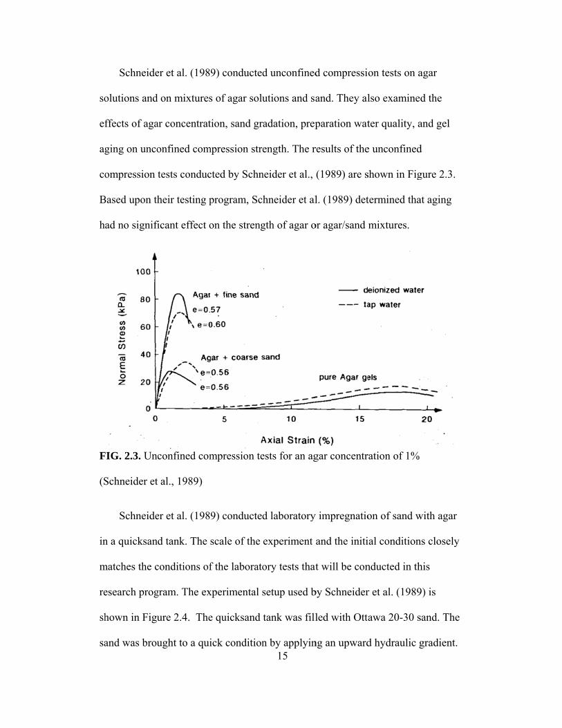
2.3. Unconfined compression tests for an agar concentration of 1%
(Schneider et al., 1989) .......................................................................... 15
2.4. Laboratory injection test in quicksand tank (Schneider et al., 1989) ..... 16
2.5. Excavated bulb after impregnation (Schneider et al., 1989) .................. 17
2.6. Agar impregnation and Flushing System (Frost, 1989) .......................... 18
2.7. Elmer's glue impregnation setup (Evans, 2005) ..................................... 20
2.8. Subsurface freezing for sampling at Fort Peck dam (Hvorslev, 1949) ... 21
2.9. Core barrel used at Fort Peck dam (Hvorslev, 1949) ............................. 22
2.10. Field and laboratory freezing setup (Yoshimi et al. 1978) ................... 23
2.11. Agarose Impregnation and Flushing System (Sutterer et al., (1995) ... 27
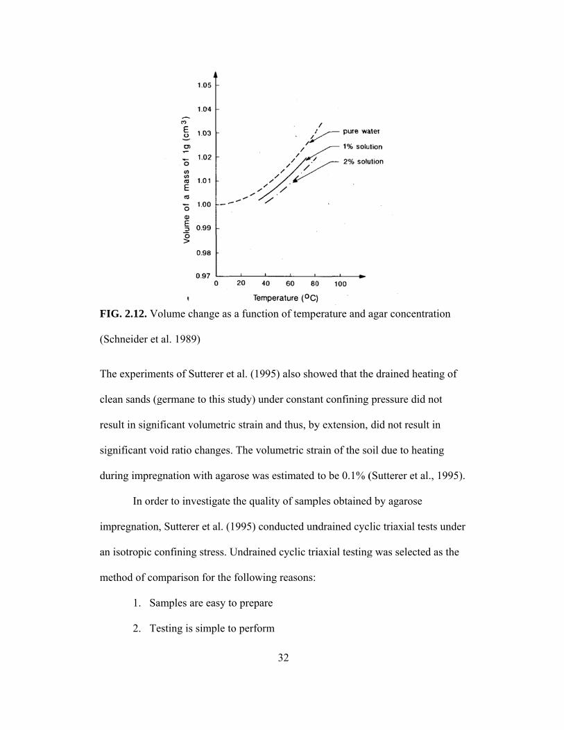
2.12. Volume change as a function of temperature and agar concentration
(Schneider et al. 1989) .......................................................................... 32
2.13. Cyclic mobility results for impregnated versus control specimens ...... 34
2.14. Gradation curves (Yoshimi et al., 1978) ............................................... 36
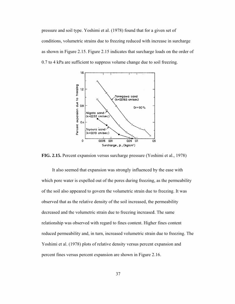
2.15. Percent expansion versus surcharge pressure (Yoshimi et al., 1978) ... 37
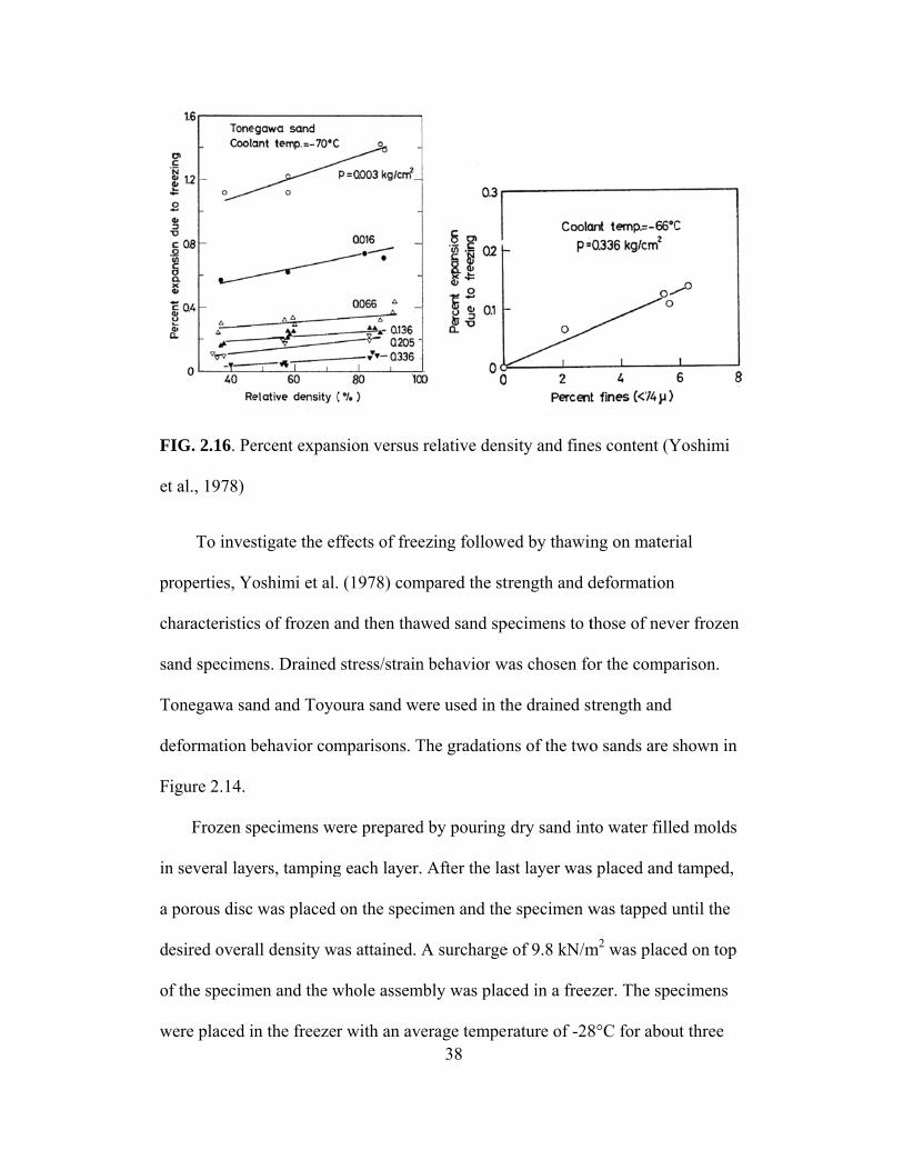
2.16. Percent expansion versus relative density and fines content (Yoshimi et
al., 1978) ............................................................................................... 38
ix
2.17. Effect of freeze thaw cycle on strength and deformation behavior ...... 40
2.18. Effect of freeze thaw cycle on friction angle ........................................ 40
2.19. Sample disturbance due to insertion of freeze pipe (Yoshimi et al.
1978) ..................................................................................................... 41
2.20. Seismic history and virgin line for never frozen specimens ................. 42
2.21. Seismic history and virgin line for frozen/ thawed specimens ............. 43
2.22. Sample preparation methods (Frost, 1989) ........................................... 44
2.23. Cylindrical tube (Mulilis et al., 1975) .................................................. 46
2.24. Tamping rod (Mulilis, 1975) ................................................................ 47
3.1. Ottawa 20-30 Gradation ......................................................................... 50
3.2. Model container (Box) ............................................................................ 52
3.3. Box Lid ................................................................................................... 52
3.4. Pluviation apparatus ................................................................................ 54
3.5. Illustration of sample preparation procedure .......................................... 56
3.6. Pluviation apparatus calibration curve .................................................... 56
3.7. Box with geonet in place ........................................................................ 57
3.8. Pluviation in progress and a completed specimen .................................. 58
3.9. Triaxial test specimen preparation Steps 1- 4 ......................................... 60
3.10. Triaxial test specimen preparation Steps 1- 7 ....................................... 61
3.11. Vacuum saturation of box specimen ..................................................... 62
4.1. Sketch of numerical model ..................................................................... 72
4.2. Numerical Modeling of Freezing Front Propagation .............................. 73
4.3. Freezing front investigation experimental setup ..................................... 75
x
4.4. Form with thermometers and frozen bulb of sand .................................. 76
4.5. Water flowing out of box during freezing .............................................. 77
4.6. Milwaukee drill, 35 mm diameter core barrel and drill guide ................ 78
4.7. Box after freezing ................................................................................... 79
4.8. Coring in progress and recovered 35 mm diameter core ........................ 79
4.9. Box and sand after coring ....................................................................... 80
4.10. Steel pipe used for 71 mm cores ........................................................... 80
4.11. Shelby tube drill adapter ....................................................................... 81
4.12. Husqvarna DR 150 core drill rig .......................................................... 81
4.13. Core drill rig adaptor ............................................................................ 81
4.14. Coring with 71 mm diameter steel pipe ................................................ 82
4.15. Large 71 mm diameter samples and specimen after sample recovery . 83
4.16. Coring with coring rig .......................................................................... 84
4.17. Sample Recovered Using Coring Rig ................................................... 85
5.1. B-value as a function of degree of saturation (Holtz & Kovacs 1981) .. 91
5.2. 71 mm diameter frozen core sample wrapped in aluminum foil ............ 94
5.3. 71 mm diameter sample preparation for testing: (a) Frozen sample after
trimming; (b) Frozen sample mounted on triaxial cell and confined in
latex membrane with vacuum confining pressure applied; (c) Frozen
sample with cell chamber in place. ........................................................ 95
5.4. Never frozen Ottawa 20-30 sand drained stress-strength-strain results . 97
5.5. Never frozen sand volume strain-axial strain results .............................. 98

xi
5.6. Results of drained triaxial compression tests on recovered frozen cores of
Ottawa 20-30 sand samples ................................................................... 99
5.7. Drained volume change-Strain results .................................................. 100
5.8. Median stress-strain-strength curves .................................................... 101
5.9. Median strain-volume change curves ................................................... 102
5.10 Never frozen Ottawa 20-30 sand undrained stress-strength-strength
results ................................................................................................... 106
5.11. Never frozen sand pore pressure change-strain results ....................... 107
5.12. Results of undrained triaxial compression tests on recovered frozen
cores of Ottawa 20-30 sand samples. ................................................... 108
5.13. Pore pressure change-axial strain results ............................................ 109
5.14. Undrained stress-strain-strength results plotted on confidence interval
developed from baseline undrained triaxial tests. ................................ 111
5.15. Median excess pore pressure-axial strain curves ................................ 111
1
Chapter 1
1.0 INTRODUCTION
The main objective of this work is to develop a method for recovering
undisturbed samples of cohesionless soil from physical models. This work is part
of a larger project to experimentally and numerically investigate the properties of
resedimented cohesionless soil following earthquake induced liquefaction (Borja
et al., 2008). Undisturbed samples of resedimented soil are required for
laboratory stress-strain-strength tests and microstructural evaluations to achieve
the project objectives.
To mitigate adverse effects of sample disturbance, cohesionless soils have to
be stabilized prior to sampling. However, in order to conduct laboratory stress-
strain-strength tests on the recovered samples, the stabilization method must be
reversible. In this work, reversible methods of obtaining undisturbed samples of
cohesionless soil are reviewed for application to the previously mentioned project.
The technique selected for obtaining undisturbed samples of cohesionless soil
from laboratory bench scale models for the larger project is described herein in
detail. And finally, the quality of samples obtained using the selected method is
evaluated using triaxial compression tests conducted on recovered samples.
1.1 Objectives
The objective of this study was to develop a method of obtaining undisturbed
samples of cohesionless soil in order to evaluate their stress-strain-strength
2
properties and micro-structure (through post-stabilization imaging). In fulfilling
this main objective, the following tasks were performed:
1. A practical method for preparing uniform soil deposits for the shake table
and centrifuge tests to be conducted in the overall research program was
developed.
2. A practical method of recovering intact and undisturbed samples of
cohesionless soil from the physical models at the scale of models used for
shake table and dynamic centrifuge experiments was developed.
3. The undisturbed nature of the intact samples recovered from physical
models was investigated using triaxial compression tests.
1.2 Background
Extensive research has been performed on the process of earthquake induced
liquefaction. However, the reverse process of resedimentation following
liquefaction has received little attention. Earthquake induced liquefaction occurs
when a soil with a well-defined soil skeleton subject to seismic loading undergoes
changes and eventually behaves like a fluid. The process of resedimentation
occurs when the soil particles in apparent suspension settle to once again form a
well-defined soil skeleton. Much attention has been paid to studying liquefaction,
as evidenced by the amount of information in the literature on the processes of
liquefaction. Studies on resedimentation subsequent to liquefaction, however, are
very rare.

3
The process of resedimentation generally involves different mechanisms
from those involved in the processes of initial formation of a soil deposit, e.g.
aeolian or alluvial deposition (Borja et al. 2008). Therefore, the structure of the
resedimented soil is likely to be significantly different from the initial soil
structure. Due to changes in structure, the resedimentation process may be
expected to have profound effects on the properties of the soil. Subsequent to
liquefaction, properties of the resedimented soil that may change include shear
strength and stiffness. Both of these properties are expected to be related to the
structure of the soil.
It is hypothesized by Borja et al. (2008) that resedimented soil has a
heterogeneous structure, i.e. when a cohesionless soil liquefies, it is unlikely to
settle into a homogenous structure and that this heterogeneous structure
contributes to the post-liquefaction properties of the soil. The resulting
heterogeneity could be of two types. The first type is due to non-uniform void
ratio distribution, for example the presence of pockets of loose sand. The second
type of heterogeneity is due to non-uniform particle gradation, for example, larger
particles settling out faster than smaller particles.
The Borja et al. (2008) hypothesis regarding the post-liquefaction
heterogeneity of soil will be investigated through an experimental program that
will include shake table testing, dynamic centrifuge testing, micro-structural
imaging tests, and laboratory stress-strain strength tests. Shake table and dynamic
centrifuge testing will be used to liquefy soil layers. Undisturbed samples will be
recovered from the liquefied soil layers. Imaging and laboratory tests will be

4
conducted on the post-liquefaction cohesionless samples recovered from shake
table and centrifuge tests. Imaging will include X-ray computed tomography
(XCT) and Bright Field Microscopy (BFM) on specimens solidified with optical
grade epoxy subsequent to freezing. Laboratory tests will include triaxial
compression tests on thawed specimens recovered from the physical models.
Special recovery techniques will be required to preserve the structure and
properties of the soil specimens recovered following liquefaction.
The techniques required to preserve the structure and properties of specimens
of resedimented soil are the subject of this thesis. The quality of samples obtained
from the physical models is paramount to the accuracy of the structural and stress-
strain-strength evaluations performed on them. The imaging that will be
conducted on recovered specimens will attempt to quantify the micro-structure of
the resedimented soil. It is imperative that the sampling process does not change
the microstructure from what it is subsequent to liquefaction. The study of
heterogeneity of the resedimented soil cannot be performed on samples whose
micro-structure in not preserved through the sampling process. The effect of
disturbance on stress-strain-strength test is well documented in the literature. The
disturbance effects must be minimized to obtain an accurate representation of the
in situ stress-strain-strength behavior. The role of this study on the previously
described larger project is to develop a reversible method of obtaining
undisturbed samples from the physical centrifuge and shake table models for
evaluation of stress-strain-strength properties and micro-structure.
5
1.3 Scope of work
Reversible stabilization methods for recovering undisturbed specimens of
cohesionless soil for subsequent imaging and testing were reviewed in the initial
phase of this study. Methods for preparing uniform soil deposits were also
reviewed. Following the review of sample preparation methods, air pluviation was
selected as the preferred technique. Following the review of methods, stabilization
by freezing and sampling by coring was selected as the preferred method. Based
on the previous research on sampling by freezing, a sampling method specific to
this work was developed. The process developed and described in this work was
designed for recovery of samples from physical models on the scale of shake table
and centrifuge tests. Samples of cohesionless soil were successfully recovered
from bench top models.
Following the development of specimen preparation, freezing, and sample
recovery techniques, triaxial compression tests were performed on thawed
specimens to demonstrate that the stress-strain-strength behavior of recovered
samples was unaffected by the stabilization and sampling processes. A series of
triaxial compression tests were performed on never frozen samples to provide a
basis for comparison to the samples recovered using the techniques developed in
this work. The test procedures and comparison results on never frozen and frozen
and thawed samples are described in this work.

6
1.4 Organization of Thesis
This thesis is organized into the following five chapters including this
introductory chapter:
Chapter 1 provides a brief background of the project to investigate the
properties of cohesionless soil subsequent to liquefaction and how the project is
related to the work presented in this thesis. The objectives, scope of the study and
outline of the thesis are also included in this chapter.
Chapter 2 presents a review of the existing technical literature on the subject
of undisturbed sampling of cohesionless soil. A review of reversible stabilization
methods, including the use of sampling using biopolymers, Elmer’s glue and
freezing, is presented. Also presented in this chapter is a review of testing and
analyses performed subsequent to stabilization and sampling to demonstrate the
quality of samples obtained from the reviewed methods.
Chapter 3 presents descriptions of methods for preparation of cohesionless
samples for laboratory testing. In this chapter, deposition methods for creating
reconstituted samples of cohesionless soils and densification methods are
described. Also presented in this chapter are the published properties of Ottawa
sand.
Chapter 4 presents development of the technique to recover undisturbed
samples of cohesionless soil for evaluation of mechanical properties and
microstructure within the context of the larger project. Challenges encountered
during the development of the technique are discussed in this chapter.

7
Chapter 5 presents the results of the tests performed to evaluate the quality of
samples obtained using the developed sampling method. The results are analyzed
and interpreted to reach reasonable conclusions.
Chapter 6 summarizes findings of the present work. Recommendations for
future work in this area of research are also presented here.

8
Chapter 2
2.0 LITERATURE REVIEW
2.1 Introduction
Sampling of soil for laboratory testing has been a subject of interest since
the early days of modern geotechnical engineering. The quality
(representativeness) of laboratory test results for evaluating stress-strain-strength
properties of soil, and by extension the quality of engineering evaluations based
on these results, is dependent on the quality of samples obtained for these tests.
Thus the objective for recovery of samples for laboratory evaluation of
mechanical properties (stress-strain-strength properties) is to recover undisturbed
samples. However, some level of disturbance during sampling may be inevitable
due to 1) the changes in the stress state of soil that are created by removal of
overburden and 2) particle reorientation from mechanical effects of sampling
(pushing a sample tube in the ground). The less disturbed a sample is, the more
closely the lab results reflect its in situ behavior.
According to Hvorslev (1949), “Undisturbed samples may be defined
broadly as samples in which the material has been subjected to so little
disturbance that it is suitable for all laboratory tests and thereby for approximate
determination of strength, consolidation, and permeability characteristics and
other physical properties of the material in situ”.
Hvorslev (1949) suggested the following criteria for assessing the quality
of relatively undisturbed samples suitable for laboratory tests:
1. No disturbance of the soil structure.

9
2. No change in water content or void ratio.
3. No change in constituents or chemical composition.
Mitchell (2008) has shown that freshly deposited cohesionless soil gains
strength with time with no apparent disturbance to structure, void ratio change, or
change in constituents, adding another dimension to the problem.
In geotechnical engineering, soils are typically divided into two broad
categories: cohesive soils and cohesionless soils. Undisturbed sampling of
cohesive soil is easier to achieve due to the internal cohesion of the cohesive soil
(i.e. the resistance of the particles to rearrangement). Current methods for
recovery of relatively undisturbed samples of cohesive soils generally employ thin
walled Shelby tubes that are pushed into the soil at a slow rate or block samples
obtained from test pits. The highest quality Shelby tube samples are generally
recovered using ‘fixed piston’ types of samplers, e.g. Osterberg or Swedish foil
samplers. Undisturbed samples of cohesive soils can also be obtained from large
block samples cut out of the wall of test pits. However, but the depth from which
such samples can be recovered is limited.
Recovery of undisturbed samples of cohesionless soils presents different
problems compared to the recovery of undisturbed samples of cohesive soils due
to the lack of internal cohesion to hold cohesionless soil particles together during
sampling and transportation. It is difficult to recover undisturbed samples of
cohesionless soil. Cohesionless soils have very little internal cohesion and thus
the particles are subject to rearrangement (change in structure) during sampling.
10
In practice, samples of cohesionless soils are obtained using drive samplers.
These samples are far from undisturbed. Their use is generally limited to
laboratory index and classification tests, such as gradation and moisture content
that are not sensitive to soil structure. Undisturbed sampling of cohesionless soil
is not normally performed in practice. Geotechnical engineers rely on in-situ tests
(such as the standard penetrometer tests) and empirical correlations to develop
estimates of the undisturbed properties of cohesionless soil. A variety of methods
may be used to obtain samples of cohesionless soil for classification and gradation
tests. However, recovery of quality samples of cohesionless soils for micro-
structure studies and stress-strain-strength determination is a difficult task.
Recovery of undisturbed samples of cohesionless soil is usually attempted only
for research purposes and is not typically attempted on routine geotechnical
projects.
Several researchers have proposed methods to recover undisturbed
samples of cohesionless soil for micro-structure studies and stress-strain-strength
determination (Frost, 1982; Hvorslev, 1949; Schneider et al., 1989; Singh et al.,
1982; and Yoshimi et al., 1978). The general procedure employed by most of
these researchers is to first stabilize the soil, next extract the sample, and then
remove (reverse) the stabilizing agent after transportation, trimming, and
confining the specimen in a testing device. Reversible stabilization methods that
have been investigated include biopolymers agar and agarose, Elmer’s glue, and
freezing. A review of each of these stabilization methods and its ability to produce
undisturbed samples is presented herein.
11
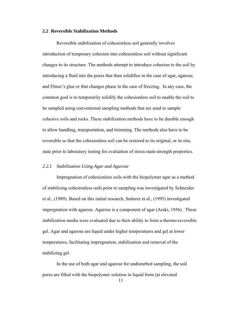
2.2 Reversible Stabilization Methods
Reversible stabilization of cohesionless soil generally involves
introduction of temporary cohesion into cohesionless soil without significant
changes to its structure. The methods attempt to introduce cohesion to the soil by
introducing a fluid into the pores that then solidifies in the case of agar, agarose,
and Elmer’s glue or that changes phase in the case of freezing. In any case, the
common goal is to temporarily solidify the cohesionless soil to enable the soil to
be sampled using conventional sampling methods that are used to sample
cohesive soils and rocks. These stabilization methods have to be durable enough
to allow handling, transportation, and trimming. The methods also have to be
reversible so that the cohesionless soil can be restored to its original, or in-situ,
state prior to laboratory testing for evaluation of stress-stain-strength properties.
2.2.1 Stabilization Using Agar and Agarose
Impregnation of cohesionless soils with the biopolymer agar as a method
of stabilizing cohesionless soils prior to sampling was investigated by Schneider
et al., (1989). Based on this initial research, Sutterer et al., (1995) investigated
impregnation with agarose. Agarose is a component of agar (Araki, 1956). These
stabilization media were evaluated due to their ability to form a thermo-reversible
gel. Agar and agarose are liquid under higher temperatures and gel at lower
temperatures, facilitating impregnation, stabilization and removal of the
stabilizing gel.
In the use of both agar and agarose for undisturbed sampling, the soil
pores are filled with the biopolymer solution in liquid form (at elevated
12
temperature). Upon cooling, the biopolymer solidifies within the pores,
introducing enough rigidity to the soil that it can be sampled without particle
rearrangement. The stabilized sample is then transported to the laboratory,
trimmed and stored (or stored and then trimmed). During laboratory testing, the
stabilized undisturbed sample is placed and confined in a testing device prior to
removal of the solidified biopolymer. Then the biopolymer is removed by heating
and flushing; thus restoring the soil to its original state as a cohesionless material.
Solubility in water and the relationship between consistency and
biopolymer temperature is the basis for the use of agar and agarose as reversible
stabilizing agents. Agar and agarose are both soluble in water. Solutions of agar
and agarose in water are prepared by boiling the dry biopolymer in water, with a
resulting viscosity that is dependent on biopolymer concentration. This solution
stays in the liquid state until a certain temperature is reached, after which the
solution turns into a rigid gel. The temperature at which the biopolymer solution
turns into a gel is called the gelation temperature. The resulting gel shows
temperature hysteresis, i.e. it remains stable at temperatures well above the
gelation temperature. This temperature hysteresis means that agar remains in
liquid form at temperatures above gelation temperature and also remains a stable
gel at temperatures below the gel melting temperature. Due to temperature
hysteresis, a properly constituted agar or agarose gel will not melt during
transportation, trimming and handling.
Gelation and gel melting temperatures are functions of the concentration
of biopolymer, the source of the biopolymer, and the extraction process (for

ag
F
(S
ag
an
pr
S
so
av
te
ag
3
an
F
garose). The
igure 2.1 as
Schneider et
gar is depen
nd agar sour
roperties dep
imilarly, the
ource agar, a
vailable with
emperatures
garose, the t
0°C at 1.5%
nd agarose a
FIG. 2.1. Gel
e variation of
determined
al. 1989). F
dent on the s
rce has been
pend upon it
e properties o
and the proce
h gelation te
ranging from
ype used by
% concentrati
are comparab
lation tempe
f gelation tem
from viscos
Figure 2.1 als
source. This
attributed to
ts origin and
of agarose ar
ess of separa
mperatures r
m ≤50°C to ≥
y Sutterer et a
on by weigh
ble.
erature versu
13
mperature an
sity tests usin
so shows tha
relationship
o the fact tha
d time of harv
re a function
ation from ag
ranging from
≥90°C (Sutt
al. (1995), h
ht in water. T
us agar conce
nd agar conc
ng a rotation
at the gelatio
p between ge
at agar is a n
vest (Schnei
n of impuriti
gar. Agarose
m 8°C to ≥42
terer, et al., 1
has a gelation
The gelation
entration (Sc
centration is
nal viscosime
on temperatu
elation temp
natural produ
ider et al., 19
ies, mixing, t
e is currently
2°C and gel-
1995). SeaPl
n temperatur
temperature
chneider et a
shown in
eter
ure of
perature
uct and its
989).
the
y
-melting
laque
re of 26-
es of agar
al., 1989)

is
te
ag
so
ra
p
ap
w
co
to
th
F
by
The ab
s governed b
emperature,
gar solution
olutions of 0
ange of temp
enetrated the
pproximately
Sutter
were used in
onstituent of
o agarose. It
hat reported
FIG. 2.2. Sol
y weight (Sc
bility of a flu
by its viscosi
and viscosity
of 0.5 % by
0.5 % by wei
perature, a lo
e pores in a s
y the same t
rer et al. (199
their experim
f natural aga
may be assu
by Schneide
lution viscos
chneider et a
uid to penetr
ity. The relat
y is shown in
y weight in th
ight have a d
ow enough v
sandy soil. T
temperature r
95) did not d
ments. Howe
ar and the use
umed that th
er et al. (198
sity versus te
a., 1989)
14
rate soil pore
tionship betw
n Figure 2.2
heir work. Fi
dynamic visc
viscosity that
The dynamic
range varies
discuss the v
ever, as men
e of agar as
e viscosity o
9) for agar.
emperature a
es under a lo
ween agar co
2. Schneider
igure 2.2 sho
cosity of 2 to
t the biopoly
c viscosity o
s between 0.6
viscosity of a
ntioned abov
a stabilizatio
of agarose is
as a function
ow hydraulic
oncentration
et al. (1989)
ows that aga
o 4 cps over
ymer solution
f water over
6 and 0.4 cp
agarose solut
ve, agarose is
on agent is a
s of the same
n agar concen
c gradient
n,
) used an
ar
a wide
n easily
r
ps.
tions that
s a
attributed
e order as
ntration
so
ef
ag
co
B
h
F
(S
in
m
re
sh
sa
Schneide
olutions and
ffects of aga
ging on unco
ompression
Based upon th
ad no signifi
FIG. 2.3. Unc
Schneider et
Schneide
n a quicksan
matches the c
esearch prog
hown in Figu
and was brou
er et al. (198
d on mixtures
ar concentrat
onfined com
tests conduc
heir testing p
ficant effect o
confined com
al., 1989)
er et al. (198
d tank. The
conditions of
gram. The ex
ure 2.4. The
ught to a qui
9) conducted
s of agar solu
tion, sand gr
mpression stre
cted by Schn
program, Sc
on the streng
mpression te
9) conducted
scale of the
f the laborato
xperimental s
e quicksand
ick condition 15
d unconfined
utions and sa
adation, prep
ength. The r
neider et al.,
hneider et al
gth of agar o
ests for an ag
d laboratory
experiment
ory tests that
setup used b
tank was fill
n by applyin
d compressi
and. They al
paration wat
results of the
(1989) are s
l. (1989) det
or agar/sand
gar concentr
y impregnatio
and the initi
t will be con
by Schneider
led with Ott
ng an upward
on tests on a
lso examined
ter quality, a
e unconfined
shown in Fig
termined tha
mixtures.
ration of 1%
on of sand w
ial condition
nducted in th
r et al. (1989
awa 20-30 s
d hydraulic g
agar
d the
and gel
d
gure 2.3.
at aging
with agar
ns closely
his
9) is
sand. The
gradient.

A
w
in
th
re
in
th
co
lo
th
O
F
An injection t
was still in th
n place. It se
he disturbanc
esedimentati
njected into t
he sand in th
oncentration
ow hydraulic
hen the soil w
Ottawa sand.
FIG. 2.4. Lab
tube and sev
he quick cond
ems that this
ce to the rese
ion, but prior
the sand at a
he vicinity of
n by weight a
c gradient. T
was sampled
boratory inje
veral small p
dition. The u
s insertion p
edimented so
r to introduc
a low hydrau
f the injectio
at 80°C were
The agar solu
d. Figure 2.5
ection test in
16
plastic tubes
upward flow
procedure wa
oil caused by
cing the agar
ulic gradient
on tube. Dyed
e then inject
ution was all
shows an ex
n quicksand t
were inserte
w was stoppe
as employed
y the insertio
r solution, w
to increase t
d agar soluti
ted through t
lowed to coo
xcavated bu
tank (Schnei
ed in the sand
ed after the tu
d in order to r
on of the tub
water at 90°C
the temperat
ions at 0.5%
the injection
ol and solidif
ulb of agar st
ider et al., 19
d while it
ubes were
reduce
bes. After
C was
ture of
% to 1.5%
n tube at
fy and
abilized
989)

F
ex
F
o
th
S
sa
by
p
th
FIG. 2.5. Exc
The follo
xperiment co
1. The a
2. The s
posse
3. Temp
the so
symm
A labo
rost (1989).
f the device
he Frost (198
utterer et al.
amples by dr
y Mulilis et
luviation app
he creation o
cavated bulb
owing conclu
onducted by
agar solution
solution soli
essed enough
perature mea
olution coul
metric transi
oratory devi
This device
is shown in
89) system to
(1995) prep
ry pluviation
al. (1975). T
paratus deve
of reproducib
b after impre
usions were
y Schneider e
n effectively
dified in the
h strength an
asurements d
d be predicte
ent heat flow
ce for agar i
e was based o
Figure 2.6.
o create agar
pared Ottawa
n using a mo
The sample p
eloped by Fr
ble cylindric
17
egnation (Sch
reached from
et al. (1989):
y penetrated a
e tank after c
nd stiffness t
demonstrate
ed from finit
w condition.
mpregnation
on a modifie
Sutterer et a
rose impregn
a 20-30 and
odification o
preparation m
rost (1989). T
cal samples o
hneider et al
m the labora
:
and displace
cooling. The
to be sample
d that the ra
te-element a
n and flushin
ed triaxial te
al. (1995) us
nated sampl
modified Ot
f the ‘raining
method invo
The pluviati
of cohesionle
l., 1989)
atory impreg
ed the pore w
impregnated
ed and handl
adius of pene
analyses of a
ng was deve
st cell. A sch
sed a later ve
es in the lab
ttawa F-125
g’ method d
olved the use
on apparatus
ess soil with
gnation
water.
d sand
led.
etration of
axis-
loped by
hematic
ersion of
boratory.
sand
described
e of a
s allows
h similar

v
to
b
an
ac
T
F
co
oid ratio and
o 20 kPa prio
iopolymer st
nd back pres
chieved. Cyc
The results of
FIG. 2.6. Aga
Labor
onducted by
d structure. T
or to impreg
tabilization m
ssure saturat
clic mobility
f this testing
ar impregnat
ratory impreg
y Sutterer et a
The samples
nation, cooli
media. The s
tion techniqu
y tests were t
g are presente
tion and Flu
gnation of p
al., (1995) in
18
were subjec
ing and gela
samples wer
ues until a B
then perform
ed subsequen
ushing System
luviated sam
n their labora
cted to confi
ation, heating
re then satur
-value of gre
med on the sa
ntly in this t
m (Frost, 19
mples with ag
atory agaros
ining pressur
g and flushin
rated using v
eater than 0.
aturated sam
thesis.
989)
garose was
se flushing a
res of 15
ng the
vacuum
.95 was
mples.
and
19
impregnation system. This system is shown in Figure 2.6. The soil was heated in a
hot bath to temperatures above the gelation temperature of the agarose solution.
The heated agarose was then introduced into the soil sample at a differential
pressure (from top to bottom) of about 10 kPa. Impregnation temperatures were
on the order of 48 to 53°C (Sutterer et al. 1995). Upon cooling, the agarose gelled,
resulting in enough cohesion to hold the sample together without a confining
pressure. The triaxial cell was taken apart, the specimen removed, and the end
platens of the cell were cleaned. The removed specimen was assumed to represent
a recovered cohesionless sample impregnated with agarose. The agarose
impregnated specimen was then remounted into the agar impregnation and
flushing system and confined. The agarose was then flushed from the specimen
for triaxial shear tests as described subsequently in this thesis.
2.2.2 Stabilization Using Elmer’s Glue
Elmer’s glue, also known as Carpenter’s glue, has also been used to stabilize
cohesionless soil for sampling. Elmer’s glue is soluble in water; therefore, the
stabilization process can be reversed. Yang (2002) and Evans (2005) used Elmer’s
glue in a two stage process for preserving the microstructure of sand specimens
tested in triaxial and biaxial shear for the purpose of quantitatively studying
internal soil microstructure in regions of high localized strain. Elmer’s glue was
used to stabilize the soil samples prior to permanently fixing them with epoxy.
This two stage process was used, in part, to avoid introducing epoxy into
equipment that the researcher wanted to save and reuse.
F
so
to
in
to
w
th
th
w
cu
w
4
F
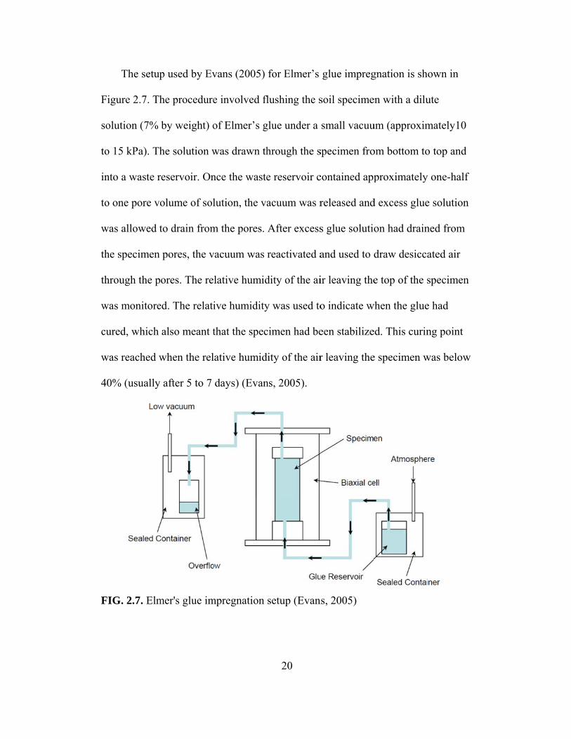
The setup
igure 2.7. Th
olution (7%
o 15 kPa). Th
nto a waste r
o one pore vo
was allowed t
he specimen
hrough the p
was monitore
ured, which
was reached w
0% (usually
FIG. 2.7. Elm
p used by Ev
he procedure
by weight) o
he solution w
reservoir. On
olume of sol
to drain from
pores, the v
ores. The re
ed. The relati
also meant t
when the rel
after 5 to 7
mer's glue im
vans (2005)
e involved fl
of Elmer’s g
was drawn th
nce the waste
lution, the va
m the pores.
vacuum was
lative humid
ive humidity
that the spec
lative humid
days) (Evan
mpregnation
20
for Elmer’s
flushing the s
glue under a
hrough the s
e reservoir c
acuum was r
After excess
reactivated a
dity of the ai
y was used to
cimen had be
dity of the air
ns, 2005).
setup (Evan
glue impreg
soil specime
small vacuu
specimen fro
contained app
released and
s glue solutio
and used to d
ir leaving the
o indicate w
een stabilize
r leaving the
ns, 2005)
gnation is sh
en with a dilu
um (approxim
om bottom to
proximately
d excess glue
on had drain
draw desicca
e top of the s
when the glue
ed. This curin
e specimen w
hown in
ute
mately10
o top and
y one-half
e solution
ned from
ated air
specimen
e had
ng point
was below

2
ob
A
fr
ci
as
co
2
sa
F
.2.3 Stabil
Samplin
btaining und
Army Corps o
reezing at Fo
irculating a f
s shown in F
ore barrel w
.9. Accordin
amples was
FIG. 2.8. Sub
lization Usin
ng by freezin
disturbed sam
of Engineers
ort Peck Dam
freezing mix
Figure 2.8. S
ith metal tee
ng to Hvorsle
‘excellent’.
bsurface free
ng Freezing
ng has long
mples of satu
s obtained in
m (Hvorslev
xture through
Samples wer
eth (Hvorslev
ev (1949), b
ezing for sam
21
been consid
urated sands
ntact samples
, 1949). Free
h seven pipe
re then obtai
v, 1949). Th
ased on visu
mpling at Fo
dered a reliab
s (Singh et al
s of cohesion
ezing was ac
es installed a
ined by corin
he core barre
ual inspectio
rt Peck dam
ble means of
l.1982). The
nless soil us
chieved by
around the bo
ng with a 91
el is shown in
n, the qualit
m (Hvorslev,
f
e US
sing
orehole,
4 mm
n Figure
ty of the
1949)

F
re
ef
fr
Fig. 2.9. Core
Sampli
ecovery of li
Yoshim
1.
2.
3.
4.
Yoshi
ffects of free
ront in the fo
e barrel used
ing by freezi
iquefiable sa
mi et al. (197
Inserting a
soil from i
installation
After the d
tube and r
Inserting a
into the tu
Pulling ou
it.
imi et al. (19
ezing on the
orm of a mix
d at Fort Peck
ing was also
ands for labo
78) proposed
an open end
inside the tu
n of self-bor
desired depth
emoving wa
a smaller vin
ube (to freeze
ut the steel tu
978) conduct
properties o
xture of ethan
22
k dam (Hvor
o researched
oratory testin
d a field samp
steel tube in
be as it pene
ring pressure
h is reached,
ater from ins
nyl tube in th
e the surroun
ube with a co
ted laborator
of the sand. T
nol and dry i
rslev, 1949)
by Japanese
ng (Yoshimi
pling proced
nto the groun
etrates (in a m
e meters).
, plugging th
side the tube
he steel tube
nding soil).
olumn of fro
ry experimen
The setup co
ice applied t
)
e investigato
et al., 1978)
dure consisti
nd and remo
manner simi
he lower end
.
and feeding
ozen sand ad
nts to invest
onsists of a fr
to one end o
ors for
).
ing of:
ving the
ilar to
d of the
g coolant
dhered to
igate the
freezing
f a
sa
et
fr
ad
la
b
b
al
sp
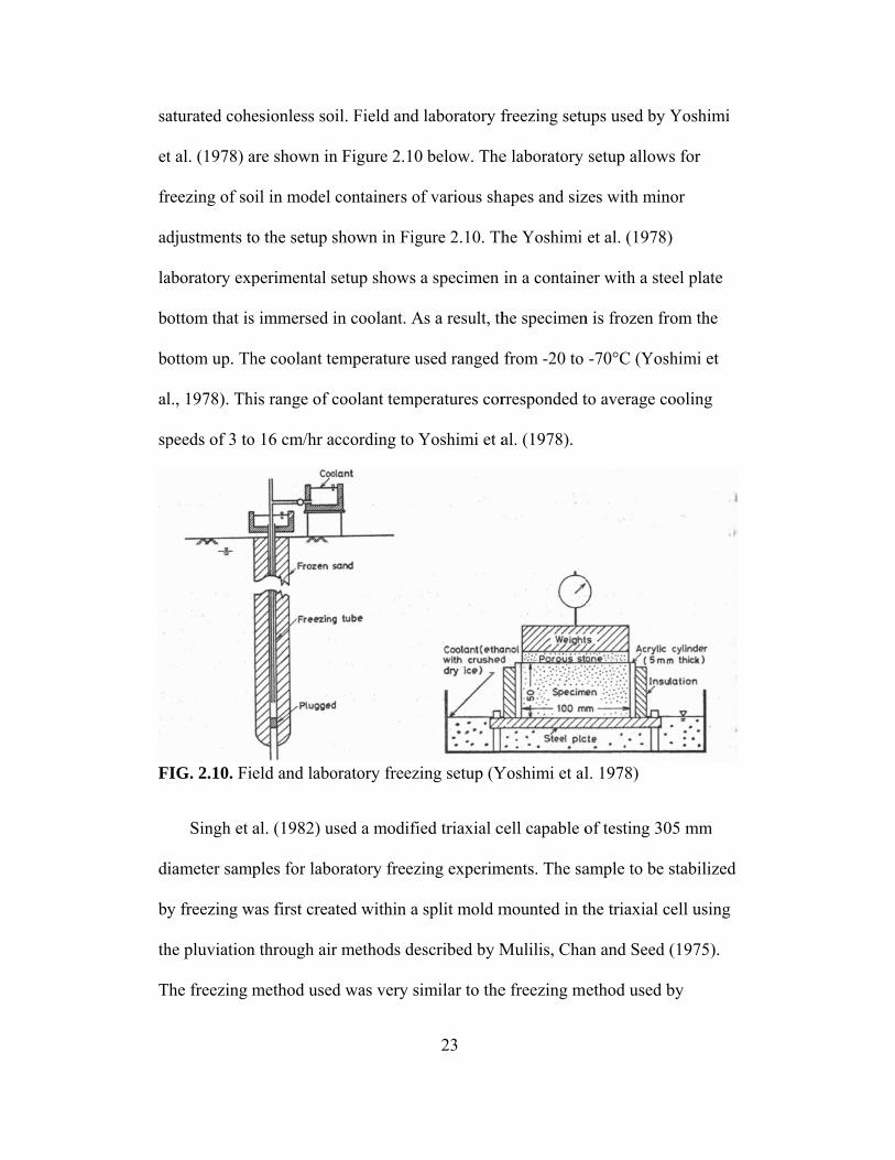
F
d
by
th
T
aturated coh
t al. (1978) a
reezing of so
djustments t
aboratory ex
ottom that is
ottom up. Th
l., 1978). Th
peeds of 3 to
FIG. 2.10. Fi
Singh et
iameter sam
y freezing w
he pluviation
The freezing
esionless so
are shown in
oil in model
o the setup s
perimental s
s immersed i
he coolant te
his range of c
o 16 cm/hr a
ield and labo
al. (1982) us
mples for labo
was first crea
n through air
method used
il. Field and
n Figure 2.10
containers o
shown in Fig
setup shows
in coolant. A
emperature u
coolant temp
ccording to Y
oratory freez
sed a modifi
oratory freez
ated within a
r methods de
d was very s
23
d laboratory f
0 below. The
of various sh
gure 2.10. Th
a specimen
As a result, th
used ranged
peratures cor
Yoshimi et a
zing setup (Y
ied triaxial c
zing experim
split mold m
escribed by M
similar to the
freezing setu
e laboratory
hapes and siz
he Yoshimi
in a contain
he specimen
from -20 to
rresponded t
al. (1978).
Yoshimi et al
cell capable o
ments. The sa
mounted in t
Mulilis, Cha
e freezing m
ups used by Y
setup allows
zes with min
et al. (1978)
er with a ste
n is frozen fr
-70°C (Yosh
to average co
l. 1978)
of testing 30
ample to be s
the triaxial c
an and Seed (
ethod used b
Yoshimi
s for
nor
)
eel plate
om the
himi et
ooling
05 mm
stabilized
cell using
(1975).
by

24
Yoshimi et al. (1978) in that the coolant was ethanol with crushed dry ice, except
that in this case, the coolant was placed on top of a modified triaxial cell top
platen, resulting in top to bottom freezing direction. The top cap of the triaxial cell
was modified to be capable of containing ethanol and crushed dry ice. Testing of
the frozen specimens after thawing is described subsequently in this thesis.
2.3 Methods for Sampling Stabilized Soil
2.3.1 Sampling Agar/Agarose Stabilized Soil
The consistency of agar impregnated soil was described by Schneider et
al. (1989) as similar to medium clay. This description agrees with the unconfined
compression test results performed on agar impregnated sand samples. It may be
assumed that agarose impregnated samples most likely have similar consistency.
The results of the unconfined compressive strength tests on agar and agar
impregnated soil are shown in Figure 2.3.
Schneider et al. (1989) performed field impregnation tests where they
demonstrated the feasibility of recovery of agar impregnated samples in the field.
In these field tests, a thin walled 127 mm diameter Osterberg sampler was used to
recover samples. The Osterberg sampler is a thin wall hydraulic fixed piston
sampler. A piston is attached to a thin wall sampling tube and locked in place at
the head of the tube. The piston and tube are seated on the bottom of the borehole.
The tube is then unlocked from the piston and is hydraulically pushed into the soil
while the piston is held in place to obtain a sample. This sampling method is
commonly used for undisturbed sampling of soft clays. Therefore, its use for

25
sampling agar impregnated soil agrees well with the medium clay consistency
characterization. The field samples recovered by Schneider et al. (1989) could
then be tested by extruding the specimen from the sampling tube and trimming
the specimen to size.
The laboratory samples of agar impregnated soil that were recovered by
Schneider et al. (1989) from the quick sand tank can be described as block
samples. The samples were recovered by excavating unstabilized soil from around
the agar stabilized soil. This process demonstrated that agar and perhaps agarose
stabilized soil samples can also be obtained by block sampling and trimming to
the required dimensions for testing provided a sufficiently large volume of soil is
stabilized.
2.3.2 Sampling Elmer’s Glue Stabilized Soil
Elmer’s glue stabilized cohesionless soil was not sampled in the
conventional sense in the work conducted by Evans (2005) and Yang (2002), as
the stabilized specimens were laboratory test specimens. However, the Elmer’s
glue stabilized specimens were able to maintain their structure during subsequent
handling after the glue cured. The samples were removed from the glue
impregnation system and the confining membrane removed without the sample
falling apart. The consistency of the specimens was described as ‘lightly
cemented’ (Evans, 2005). It is conceivable that Elmer’s glue stabilized soil could
be sampled using block sampling, push tube methods, or even coring. However,
in the absence of specific information on the consistency or unconfined

26
compressive strength, it is hard to tell how specimens can be properly sampled
from Elmer’s glue stabilized soil.
2.3.3 Sampling Soil Stabilized by Freezing
The sampling operations at Fort Peck Dam that were conducted by the US
Army Corps of Engineers involved complete freezing of the soil below the bottom
of the borehole (Hvorslev, 1949). Samples were recovered using the single tube
0.91 m diameter core barrel with metal teeth with a calyx shown in Figure 2.9.
Field sampling of frozen soil that was conducted by Yoshimi et al. (1978)
can be best described as block sampling. The frozen sand was lifted en masse by
grabbing the freeze pipe with a crane and pulling it out of the ground. This
procedure produced a nearly uniform 0.4 m diameter cylindrical mass of frozen
sand around the freeze pipe. Smaller samples for laboratory testing were obtained
from this frozen mass by trimming from the cylindrical core.
Singh et al. (1982) did not perform any field sampling of frozen soil.
However, they did obtain samples from the soil that they froze in the 300 mm
diameter triaxial cell. The frozen 300 mm diameter specimen was removed from
the triaxial cell and carried to a radial drill press. Using a diamond core drill, 71
mm diameter cores 18 to 25 mm long were recovered from the 300 mm diameter
frozen specimen. Compressed carbon dioxide was used as the drilling fluid (Singh
et al. (1982).

2
2
by
F
fl
2
F
h
ag
re
w
te
re
.4 Remova
.4.1 Remo
Remo
y use of the
rost (1989) a
lushing syste
.11.
FIG. 2.11. Ag
To rem
ot water and
garose gel m
emoval temp
were on the o
emperature i
emoval temp
l of Stabiliz
val of Agar/A
oval of agar a
Laboratory
and Sutterer
em used by S
garose Impr
move agaros
d the confine
melting temp
peratures we
order of 90°C
s the major a
perature is si
zing Agent
/Agarose
and agarose
Agar Flushin
r et al. (1995
Sutterer et al
egnation and
se, the reserv
ed, agarose im
erature using
ere on the ord
C (Sutterer e
advantage th
ignificantly l
27
from stabiliz
ng and Impr
). The versio
l. (1995) is s
d Flushing S
voirs shown
mpregnated
g a hot bath
der of 70°C
t al., 1995).
hat agarose h
lower than th
zed samples
regnation sys
on of the aga
shown schem
System (Sutt
in Figure 2.
sample was
within the tr
and agar rem
The differen
has over aga
he boiling po
s was accomp
stem describ
ar impregnat
matically in F
terer et al., (1
11 were fille
heated to th
riaxial cell. A
moval tempe
nce in remov
ar. The agaro
oint of water
plished
bed by
tion and
Figure
1995)
ed with
he
Agarose
eratures
val
ose
r. When
28
the agarose had melted and began to flow, hot water was circulated through the
sample until the agarose was flushed out. A volume of 2,500 to 4,000 ml (equal to
approximately 4 to 7 pore volumes) of tap water circulated in one direction was
typically required for complete removal of visible evidence of agarose. Using an
earlier prototype of the system, Frost (1989) found that periods of both upward
and downward flushing was necessary to remove any visual evidence of agar.
Frost (1989) found that flushing in only one direction resulted in remnants of agar
remaining in the specimen near the platens but Sutterer et al., (1995) reported no
such problems using agarose.
2.4.2 Removal of Elmer’s Glue
Elmer’s glue is soluble is water. Evans (2005) relied on this property to
clean his equipment following the first stage of his two-stage impregnation
process. To remove the glue, he soaked Elmer’s glue filled equipment in water for
several days. After the glue had dissolved, the equipment was washed with water
to remove any glue remnants. It can be inferred that the same process can be used
to remove Elmer’s glue from soil pores. The second stage of the Yang (2002) and
Evans (2005) stabilization process was to impregnate the Elmer’s glue cemented
sample with epoxy to permanently fix the specimen. It can also be inferred from
this that Elmer’s glue stabilized samples had at least moderate permeability. The
removal process could involve:
1. Placing specimens in a triaxial cell and applying a small confining
pressure.
2. Saturating the specimen with water for a few days.

29
3. Flushing the specimen with water until all evidence of Elmer’s glue
was completely removed.
2.4.3 Restoration of Samples Stabilized by Freezing
In order to return samples stabilized by freezing to their original state, both
Yoshimi et al. (1978) and Singh et al. (1982) simply allowed the soil to thaw. The
samples were placed in a testing device (triaxial cell) and an effective confining
pressure equal to the effective confining pressure during freezing was applied to
the sample. The thawing sample was kept in contact with water during the
thawing process so that water could be drawn into the sample as the pore water
thawed and reduced in volume. The time required to completely thaw the sample
is a function of (among other things) the ambient room temperature, the size of
the sample, and the temperature of the ‘free access’ water.
2.5 Quality of Undisturbed Samples
Any consideration of a sampling process is incomplete without evaluating the
quality of samples obtained using the undisturbed sampling technique. There is no
standard method of evaluating undisturbed samples. For cohesionless soils, one
can consider the Hvorslev (1949) criteria and look at void ratio changes as
indication of volumetric strains and structure collapse. However, studies have
shown that the specimens prepared to the same void ratio but with different
preparation methods can have very different stress-strain-strength behavior
(Mulilis et al. 1975). Therefore, comparison of the stress-strain-strength behavior

30
of recovered specimens to the in situ behavior is essential to demonstrating that
the sampling method produced an undisturbed sample.
2.5.1 Quality of Agar/Agarose Stabilized Samples
The following aspects of the polymer impregnation technique for undisturbed
sampling of cohesionless soil may be considered as potential sources of
disturbance:
1. Volume change of the agar/agarose solution with changes in temperatures
including changes in volume during gelation.
2. Volume changes in the soil and pore water during heating prior to
injection of agar/agarose.
3. Disturbance from insertion of the sample tube or electrodes.
4. Effects of the agar/agarose removal process.
5. Loss of aging-induced strength gain that occurs with no discernable
volume change (Mitchell, 2008).
Since the agar will replace the pore fluid, changes in the agar volume may
result in changes in the soil void ratio, particularly if there is a volume increase.
According to Schneider et al. (1989), a dilute agar solution above the gelation
temperature exhibits the same volume change with increase in temperature as
water. The results of the laboratory volume change measurements made by
Schneider et al. (1989) on agar solutions are shown in Figure 2.12. Changes in
agar volume during gelation were also analyzed. The agar decreased in volume
upon gelation and the volume decrease of the agar during gelation was less than
2% for agar concentrations as high as 2% (Schneider et al., 1989). Gels were not
31
remelted to model the effects of agar removal. However, Schneider et al. (1989)
state that “Observations made during the melting of cubes of agar gels indicate
that the volume change effects are probably thermo reversible”.
Heating generates volume and effective stress changes in saturated soil. This
is due to the differential thermal expansion of the pore water and mineral
particles. The volume change behavior of heated soil differs for drained heat and
undrained heating. For purposes of this study, soil heating for biopolymer
impregnation can be assumed to occur under drained conditions. The subject of
soil temperature-volume relationships is discussed in great detail by Mitchell and
Soga (2005). Under drained conditions the soil grains and the soil mass undergo
the same volumetric strains. Therefore, under drained heating, pore fluid will flow
out of the heated region because, for a given temperature change, the volumetric
strain of water is greater than the volumetric strain of solid soil particles. Heating
may also induce changes in inter particle forces if the specimen is not free to
change in volume (e.g. under one dimensional conditions in the ground). Heating
a soil specimen constrained from volume change can cause changes in cohesion
and/or frictional resistance that may result in particle reorientation, and under
extreme conditions, in particle crushing. Particle reorientation is a significant
factor in soil fabric. Sutterer et al. (1995) conducted experiments using Ottawa
20-30 sand and concluded that the level of heating involved in biopolymer
impregnation did not result in particle crushing.
F
(S
T
cl
re
si
du
im
an
m
FIG. 2.12. Vo
Schneider et
The experime
lean sands (g
esult in signi
ignificant vo
uring impreg
In ord
mpregnation
n isotropic c
method of com
1. Sa
2. Te
olume chang
al. 1989)
ents of Sutte
germane to t
ificant volum
oid ratio chan
gnation with
der to investi
n, Sutterer et
confining stre
mparison fo
amples are e
esting is sim
ge as a funct
rer et al. (19
this study) un
metric strain
nges. The vo
h agarose wa
igate the qua
al. (1995) co
ess. Undrain
r the followi
asy to prepa
mple to perfor
32
tion of tempe
995) also sho
nder constan
and thus, by
olumetric str
as estimated
ality of samp
onducted un
ned cyclic tri
ing reasons:
are
rm
erature and a
owed that the
nt confining
y extension,
rain of the so
to be 0.1% (
ples obtained
ndrained cyc
iaxial testing
agar concent
e drained he
pressure did
did not resu
oil due to he
(Sutterer et a
d by agarose
lic triaxial te
g was selecte
tration
eating of
d not
ult in
ating
al., 1995).
ests under
ed as the

33
3. It has been used by other researchers (Yoshimi et al. 1984, and Mulilis
et al. 1975) for similar purposes.
A comparison of the cyclic triaxial test results on impregnated specimens and
on control specimens is shown in Figure 2.13. Sutterer et al. (1995) developed a
mathematical relationship between the Cyclic Stress Ratio (CSR) and the number
of cycles to failure, Nf, presented by the equation 2.1:
(2.1)
where b, a and c are curve fitting parameters
Based on the relationship in Equation 2.1, a comparison between
impregnated samples and control samples was made. The results of the
comparison showed that the variation between impregnated and control samples
was within the normal range of scatter expected for this type of test. The
comparison also showed that there was a slight reduction in cyclic stress
resistance or cyclic mobility after agarose impregnation and flushing. This
reduction was attributed to the slight expansion observed during drained heating
of the soil prior to sampling and also to residual agarose in the sample. Although
Sutterer et al. (1995) observed no traces of agarose in the sample after flushing
with hot water, he speculated that there was still some agarose left between the
particle contacts.

F
2
in
st
2
w
co
FIG. 2.13. Cy
.5.2 Quali
The qual
nvestigated b
tudy of the m
.5.3 Quali
Water
water were al
oncurrent in
yclic mobilit
ty of Elmer’s
lity of sampl
by either Yan
microstrustur
ty ot Freeze
r expands ap
llowed to oc
crease in vo
ty results for
s Glue Stabi
les stabilized
ng (2002) or
re of sand sp
Stabilized S
pproximately
cur without
id ratio, loss
34
r impregnate
ilized Sampl
d by Elmer’s
r Evans (200
pecimens.
Samples
y 9 % upon f
drainage, th
s of inter-par
ed versus con
les
s glue was no
05) as their w
freezing. If e
he soil mass w
rticle contac
ntrol specim
ot explicitly
work involve
expansion of
would exper
ts, and conse
mens
ed only
f soil pore
rience a
equently

35
significant disturbance. The expansion of pore water during freezing is perhaps
the main source of potential disturbance in the stabilization of cohesionless soil
for undisturbed sampling using freezing.
The question of the expansion of water during freezing and whether this
phenomenon disturbs the structure of the sand or its properties was investigated
by Hvorslev (1949), Tystovich (1952), Yoshimi et al. (1978) and Singh et al.
(1982). The main conclusion of all these investigations with regard to disturbance
due to expansion of water upon freezing was that a unidirectional freezing front,
unimpeded drainage path, and slight overburden pressure were necessary to
minimize disturbance due to water expansion upon freezing. A complete review
of the processes governing the volume change associated with freezing pore water
is beyond the scope of this study but the essential conclusions from previous
investigations are summarized below.
Hvorslev (1949) simply stated that “it is possible that the expansion of
water during freezing simply will force some of the unfrozen water out of the soil
and not change the void ratio or disturb the soil structure”. Extensive research on
the subject of freezing pore water in soil was conducted by Tystovich (1952).
According to Tystovich (1952), “it was established that in water saturated sands
with free drainage of water in at least one direction, water does not migrate
towards the freezing point, but is squeezed out, with the result that the porosity of
frozen water saturated sands remains practically the same.” A more
comprehensive study of the effect of freezing on cohesionless soil was conducted
by Yoshimi et al. (1978) who conducted one dimensional laboratory freezing

ex
th
u
o
ex
th
cr
in
F
fa
xperiments t
he soil skelet
1. S
2. S
3. R
4. C
Yoshimi e
sing three so
f the three sa
xperimental
he bottom by
rushed dry ic
nvestigate th
FIG. 2.14. Gr
The Yosh
actors on the
to examine t
ton during fr
Surcharge/ov
Soil type/Fin
Relative dens
Coolant temp
et al. (1978)
oils: Toyoura
ands are sho
setup was sh
y immersing
ce) and drain
he factors list
radation curv
himi et al. (1
e amount of v
the effects of
reezing:
verburden.
es content
sity
perature.
conducted l
a sand, Tone
own in Figur
hown in Fig
the steel bo
nage was pro
ted above.
ves (Yoshim
1978) experi
volumetric s
36
f the followi
laboratory te
egawa sand,
e 2.14. The Y
ure 2.10. Th
ottom in cool
ovided at the
mi et al., 197
iments show
strains due to
ing factors o
ests to evalua
and Niigata
Yoshimi et a
he specimens
lant (mixture
e top. This s
8)
wed that the t
o freezing w
n the expans
ate the abov
a sand. The g
al. (1978)
s were froze
e of alcohol
etup was use
two most inf
were overburd
sion of
e factors
gradations
n from
and
ed to
fluential
den
pr
co
as
0
F
w
o
ob
d
re
re
Y
p
ressure and
onditions, vo
s shown in F
.7 to 4 kPa a
FIG. 2.15. Pe
It also s
which pore w
f the soil als
bserved that
ecreased and
elationship w
educed perm
Yoshimi et al
ercent fines
soil type. Yo
olumetric str
Figure 2.15.
are sufficient
ercent expan
seemed that e
water is expel
so appeared t
t as the relati
d the volume
was observed
meability and
l. (1978) plo
versus perce
oshimi et al.
rains due to
Figure 2.15
t to suppress
nsion versus
expansion w
lled out of th
to govern the
ive density o
etric strain d
d with regard
d, in turn, inc
ts of relative
ent expansio
37
(1978) foun
freezing red
indicates tha
s volume cha
surcharge pr
was strongly
he pores duri
e volumetric
of the soil in
due to freezin
d to fines co
creased volum
e density ver
on are shown
nd that for a
duced with in
at surcharge
ange due to
ressure (Yos
influenced b
ring freezing
c strain due t
creased, the
ng increased
ontent. Highe
umetric strain
rsus percent
n in Figure 2
given set of
ncrease in su
e loads on the
soil freezing
shimi et al.,
by the ease w
g, as the perm
to freezing. I
permeabilit
d. The same
er fines cont
n due to free
expansion a
2.16.
f
urcharge
e order of
g.
1978)
with
meability
It was
ty
ent
ezing. The
and
F
et
pr
ch
sa
T
d
F
in
a
d
o
w
FIG. 2.16. Pe
t al., 1978)
To inves
roperties, Yo
haracteristic
and specime
Tonegawa san
eformation b
igure 2.14.
Frozen sp
n several lay
porous disc
esired overa
f the specim
were placed i
ercent expan
stigate the ef
oshimi et al.
s of frozen a
ens. Drained
nd and Toyo
behavior com
pecimens we
yers, tamping
was placed
all density wa
men and the w
n the freezer
nsion versus
ffects of free
(1978) com
and then thaw
stress/strain
oura sand we
mparisons. T
ere prepared
g each layer.
on the speci
as attained. A
whole assem
r with an ave 38
relative den
ezing follow
mpared the st
wed sand sp
n behavior w
ere used in th
The gradation
d by pouring
After the la
imen and the
A surcharge
mbly was plac
erage temper
sity and fine
wed by thawin
trength and d
pecimens to t
was chosen fo
he drained st
ns of the two
dry sand int
ast layer was
e specimen w
e of 9.8 kN/m
ced in a free
rature of -28
es content (Y
ng on materi
deformation
those of nev
or the compa
trength and
o sands are s
to water fille
s placed and
was tapped u
m2 was place
zer. The spe
8°C for abou
Yoshimi
ial
er frozen
arison.
shown in
ed molds
tamped,
until the
ed on top
ecimens
ut three
39
hours. This freezing method does not seem to apply a unidirectional freezing
front to the specimens. In fact, it is likely that the samples were frozen from all
directions using this technique. Yoshimi et al. (1978) do not address this issue.
The frozen specimens were placed in a triaxial cell and confining pressures of 29
to 98.1 kPa were applied. The specimens were allowed to thaw while both ends
where allowed access to water. The specimens were saturated by circulating pore
water through the thawed specimen for 24 hours under a maximum differential
head of 300 mm.
Unfrozen specimens were prepared in the same way as the frozen specimens
but without placement in the freezer. Both frozen and unfrozen specimens were
prepared at a range of relative densities between 40 and 90 percent.
Drained triaxial compression tests were conducted on the two types of
specimens (Frozen/Thawed and Never Frozen) at confining pressures of 3 to 10
kPa. A comparison of the two sets of tests is presented in Figure 2.17. The results
presented in Figure 2.17 show that the freeze/thaw cycle has only a minor effect
on the drained strength and deformation behavior of both Toyoura sand and
Tonegawa sand for specimens of the same age. The comparison of friction angles
for frozen and thawed specimens versus never frozen specimens, shown in Figure
2.18, indicates that the freeze thaw cycle has no significant effects on the friction
angle for both sands.

F
F
in
ev
on
du
fu
FIG. 2.17. Ef
FIG. 2.18. Ef
Yoshimi
nsertion of th
valuation are
ne diameter
uring inserti
unction of th
ffect of freez
ffect of freez
et al. (1978)
heir freezing
e presented i
of the tube u
ion of the fre
he initial den
ze thaw cycl
ze thaw cycl
) presented a
g tube into sa
in Figure 2.1
underwent v
eezing tube.
nsity of the s 40
e on strength
e on friction
an evaluation
aturated sand
19. It was de
void ratio cha
The changes
and. Loose s
h and deform
n angle
n of the distu
d in situ. The
etermined tha
anges due to
s in the void
samples tend
mation behav
urbance due
e results of t
at the sand w
o shearing of
d ratio were a
ded to contra
vior
e to
the
within
f the sand
a
act,

re
in
F
1
dy
ac
4
pr
co
esulting in a
n void a ratio
FIG. 2.19. Sa
978)
Singh et
ynamic stren
ccording to p
8 percent. T
ressure of 20
onducted on
void ratio d
o increase.
ample disturb
al. (1982) in
ngth of sand
procedure de
he specimen
0 kPa and a b
n one set of s
decrease, whi
bance due to
nvestigated t
d. Test specim
escribed by M
ns were then
back pressur
specimens to
41
ile dense sam
o insertion o
the effects of
mens were p
Mulilis et al
saturated an
re of 15 kPa
o establish a
mples tended
f freeze pipe
f a freeze tha
prepared by p
l. (1975) to a
nd consolida
a. Cyclic triax
virgin line. A
d to dilate, re
e (Yoshimi e
aw cycle on
pouring and
a relative den
ated under a
xial tests we
A second se
esulting
et al.
the
tamping
nsity of
cell
ere
t of

sp
tr
fi
se
m
sp
ch
B
S
co
m
un
F
pecimens wa
riaxial tests t
Two add
irst two sets,
ets of specim
modified triax
pecimens we
haracteristic
The resu
Based on com
ingh et al. (1
onditions of
movement of
ndisturbed s
FIG. 2.20. Se
as subjected
to establish a
ditional set of
, with one se
mens were th
xial cell and
ere subjected
curves.
lts of the fou
mparison of t
1982) conclu
f unidirection
f the freezing
samples of sa
eismic histor
to low ampl
a set of speci
f specimens
et subjected t
hen frozen us
d subsequentl
d to cyclic tr
ur sets of tes
the cyclic tri
uded that soi
nal freezing
g front provi
aturated sand
ry and virgin
42
litude cyclic
imens influe
were prepar
to the same s
sing a unidir
ly thawed. T
riaxial tests t
sts are shown
iaxial test res
il sampling b
and unimped
des an effec
ds.
n line for nev
c loading prio
enced by seis
red using ide
seismic histo
rectional free
Then the thir
to establish t
n in Figure 2
sults in Figu
by freezing a
ded drainage
ctive method
ver frozen sp
or to the cyc
smic history
entical metho
ory. The sec
ezing front i
rd and fourth
their cyclic
2.20 and Figu
ures 2.20 and
and coring u
e in the direc
d of obtaining
pecimens
clic
y.
ods as the
cond two
in a
h sets of
ure 2.21.
d 2.21,
under
ction of
g

F
2
pr
pr
at
b
at
(M
th
sa
an
ar
FIG. 2.21. Se
.6 Prepara
For the p
roducing sam
roperties. Th
t a desired d
oth static an
t the same de
Mililis et al.
he specimen
ame density.
nd their vari
re discussed
eismic histor
tion of Coh
purposes of t
mples of san
here are num
density descr
nd dynamic s
ensity can be
1975). For p
s with the sa
. A summary
ious compon
d below.
ry and virgin
esionless So
this project, i
nd at a desire
merous metho
ibed in the li
strength and
e influenced
purposes of t
ame properti
y of the mos
nents is prese
43
n line for froz
oil Samples
it was impor
ed density w
ods for creat
iterature. Ho
deformation
d by the meth
his study, it
es as it was
t common m
ent in Figure
zen/ thawed
for Labora
rtant to deve
with consisten
ting reprodu
owever, stud
nal propertie
hod of the sa
was just as i
to to produc
methods of sa
e 2.22. Detai
d specimens
atory Testin
elop a metho
nt, reproduci
ucible sample
dies have sho
es of sand sp
ample prepar
important to
ce samples w
ample prepa
ils about eac
g
od for
ible
es of sand
own that
ecimens
ration
o prepare
with the
aration
ch method
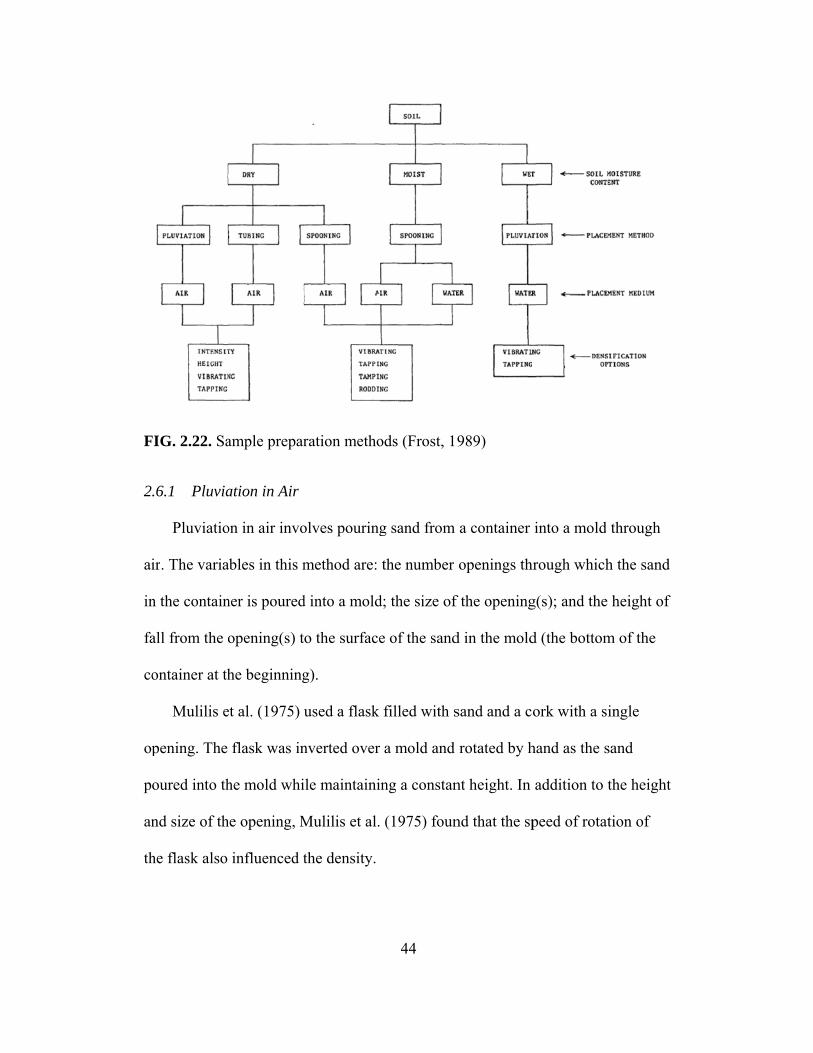
F
2
ai
in
fa
co
op
p
an
th
FIG. 2.22. Sa
.6.1 Pluvia
Pluviatio
ir. The varia
n the contain
all from the o
ontainer at th
Mulilis e
pening. The
oured into th
nd size of th
he flask also
ample prepar
ation in Air
on in air invo
ables in this m
ner is poured
opening(s) t
he beginning
et al. (1975) u
flask was in
he mold whi
he opening, M
influenced t
ration metho
olves pouring
method are:
d into a mold
o the surface
g).
used a flask
nverted over
ile maintaini
Mulilis et al.
the density.
44
ods (Frost, 1
g sand from
the number
d; the size of
e of the sand
filled with s
a mold and
ng a constan
(1975) foun
989)
a container
openings th
f the opening
d in the mold
sand and a c
rotated by h
nt height. In
nd that the sp
into a mold
hrough which
g(s); and the
d (the bottom
ork with a si
hand as the s
addition to t
peed of rotat
through
h the sand
height of
m of the
ingle
sand
the height
tion of
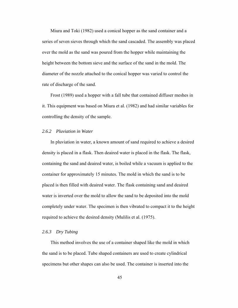
45
Miura and Toki (1982) used a conical hopper as the sand container and a
series of seven sieves through which the sand cascaded. The assembly was placed
over the mold as the sand was poured from the hopper while maintaining the
height between the bottom sieve and the surface of the sand in the mold. The
diameter of the nozzle attached to the conical hopper was varied to control the
rate of discharge of the sand.
Frost (1989) used a hopper with a fall tube that contained diffuser meshes in
it. This equipment was based on Miura et al. (1982) and had similar variables for
controlling the density of the sample.
2.6.2 Pluviation in Water
In pluviation in water, a known amount of sand required to achieve a desired
density is placed in a flask. Then deaired water is placed in the flask. The flask,
containing the sand and deaired water, is boiled while a vacuum is applied to the
container for approximately 15 minutes. The mold in which the sand is to be
placed is then filled with deaired water. The flask containing sand and deaired
water is inverted over the mold to allow the sand to be deposited into the mold
completely under water. The specimen is then vibrated to compact it to the height
required to achieve the desired density (Mulilis et al. (1975).
2.6.3 Dry Tubing
This method involves the use of a container shaped like the mold in which
the sand is to be placed. Tube shaped containers are used to create cylindrical
specimens but other shapes can also be used. The container is inserted into the
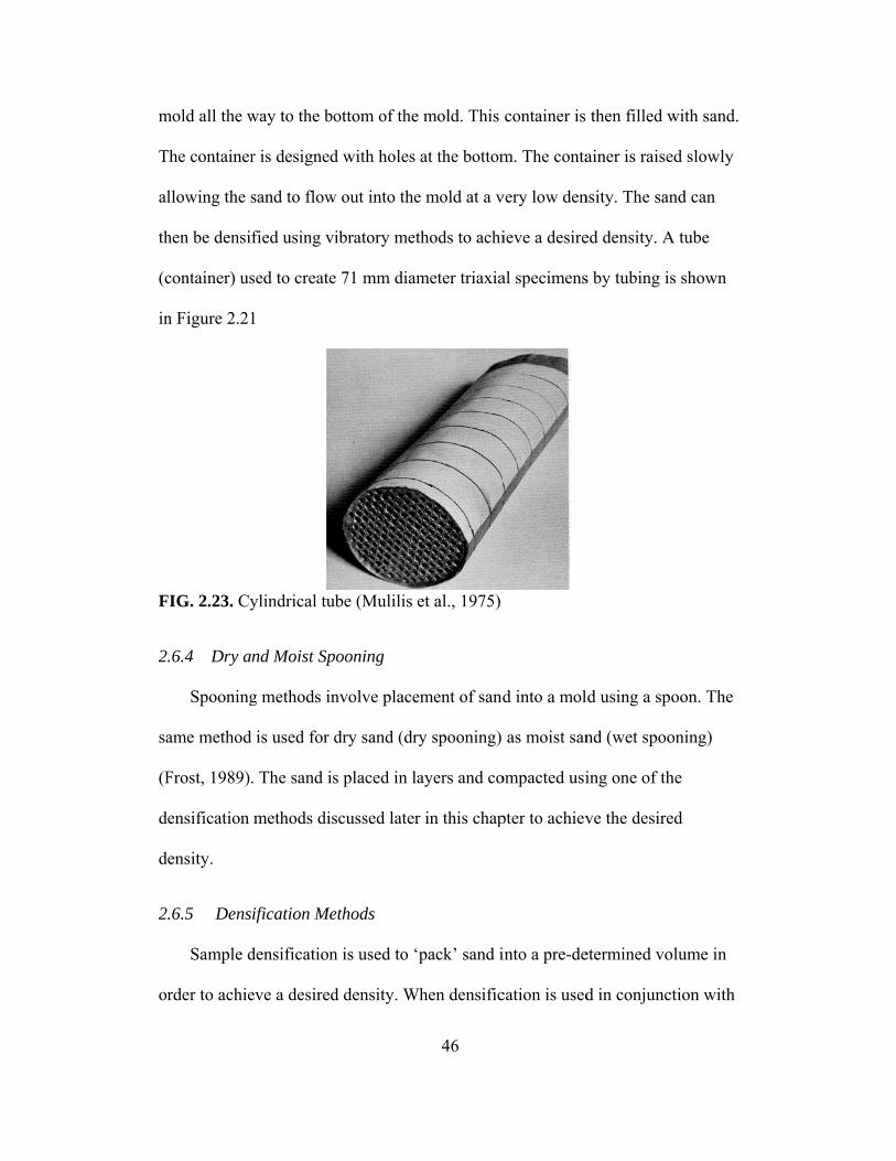
m
T
al
th
(c
in
F
2
sa
(F
d
d
2
or
mold all the w
The container
llowing the s
hen be densi
container) us
n Figure 2.21
FIG. 2.23. Cy
.6.4 Dry a
Spooning
ame method
Frost, 1989)
ensification
ensity.
.6.5 Dens
Sample d
rder to achie
way to the bo
r is designed
sand to flow
fied using vi
sed to create
1
ylindrical tub
nd Moist Sp
g methods in
d is used for d
. The sand is
methods dis
ification Me
densification
eve a desired
ottom of the
d with holes
w out into the
ibratory met
e 71 mm diam
be (Mulilis e
ooning
nvolve place
dry sand (dry
s placed in la
scussed later
ethods
n is used to ‘p
d density. W
46
mold. This
at the bottom
e mold at a v
thods to achi
meter triaxia
et al., 1975)
ement of sand
y spooning)
ayers and co
r in this chap
pack’ sand i
When densific
container is
m. The conta
very low den
ieve a desire
al specimens
d into a mol
as moist san
ompacted usi
pter to achiev
into a pre-de
cation is used
then filled w
ainer is raise
nsity. The san
ed density. A
s by tubing is
d using a sp
nd (wet spoo
ing one of th
ve the desire
etermined vo
d in conjunc
with sand.
ed slowly
nd can
A tube
s shown
oon. The
oning)
he
ed
olume in
ction with
la
co
(M
un
u
co
co
tr
pr
h
ta
F
to
ayered samp
ompacted m
Mulilis et al.
nder compac
sed. The low
ompaction o
ompaction p
rial and error
Densifica
reparation. I
eight of the
amping rod u
FIG. 2.24. Ta
Densifica
o reduce the
le preparatio
more as additi
. 1975). To m
cted by a cer
wer layer is p
of a layer usu
procedure res
r to establish
ation by tam
In this metho
layers reduc
used by Mul
amping rod (
ation by tapp
height of the
on, there is a
ional layers
mitigate this
rtain percent
prepared in t
ually ranges
sults in more
h the amount
mping is usua
od a tamping
ced enough t
lilis et al. (19
(Mulilis, 197
ping is achie
e sand in ord
47
a tendency fo
are placed a
problem, a p
tage of the fi
the loosest st
from 0-20%
e uniform sp
t of under co
ally used in c
g rod is used
o achieve a d
975) is show
75)
eved by tapp
der to achiev
or the lower
and compacte
procedure in
final desired
tate. The per
% (Mulilis et
pecimens but
ompaction fo
conjunction
d to compact
desired dens
wn in Figure
ping the spec
ve a desired
layers to be
ed on top of
n which each
compaction
rcent under
al. 1975). T
t requires sig
or each layer
with layered
a soil layer
sity. A pictur
2.22.
cimen mold r
density. The
f them
h layer is
may be
This under
gnificant
r.
d sample
until the
re of a
radially
e intensity

48
of tapping must be kept uniform throughout the specimen preparation process in
order to create uniform specimens.
Rodding involve plunging a vibrating rod in and out of the specimen starting
from the edges and working toward the center to achieve the desired density. The
surface of the specimen is then leveled by applying a small pressure using a flat
surface.
Vibrating involves vibrating the sample mold around the perimeter to densify
the specimen. Vibrating a specimen allows the particles to pack in more closely
and densify the specimen. Vibration can be used to densify a single layer or it can
be used to densify a whole specimen by apply vibrations using a hand held
vibrator at random locations along the height of the specimen.

49
Chapter 3
3.0 PROPERTIES OF TEST SAND AND SPECIMEN PREPARATION
Ottawa 20-30 sand (ASTM Designation C778), from U.S. Silica Company in
Ottawa, Illinois was selected as the test sand for all experiments in this work. The
selection was based on the fact that Ottawa 20-30 sand is readily available with
near consistent properties and has been used by many researchers for experiments
on cohesionless soil. Therefore, some of the properties of Ottawa 20-30 sand were
available in the literature.
3.1 Properties of Ottawa 20-30 Sand
Ottawa 20-30 sand is a poorly graded sand that consists of subrounded
particles and is composed primarily (99.8%) of silicon dioxide (quartz) (Evans,
2005). Numerous researchers have used Ottawa 20-30 sand for investigations
involving the use of a uniform cohesionless soil (Alshibli et al. 2000, Santamarina
and Cho 2001, Evans 2005, Salgado, et al. 2000).
3.1.1 Gradation
Gradation tests were performed in accordance with ASTM D6913 on Ottawa
20-30 sand obtained from U.S. Silica Company, Ottawa, Illinois for this project.
The gradation of the Ottawa 20-30 sand obtained for this project is shown in
Figure 3.1. The gradation results are consistent with gradations reported by other
researchers for Ottawa 20-30 sand (presented in Appendix A).

50
FIG. 3.1. Ottawa 20-30 Gradation
3.1.2 Maximum and Minimum Void Ratio
Maximum and minimum void ratios of Ottawa 20-30 sand published by other
researchers are presented in Table 1. Void ratios published by Santamarina et al.
(2001) were used calculations of minimum and maximum densities and in the
determination of relative density.
Table 3-1. Ottawa 20-30 Sand Maximum and Minimum Void ratio
Maximum Void Ratio Minimum Void Ratio Reference
0.81 0.49 Alshibli et al. (2000)
0.742 0.502 Santamarina et al. (2001)
0.78 0.48 Salgado et al. (2000)
0%
10%
20%
30%
40%
50%
60%
70%
80%
90%
100%
0.01 0.1 1 10 100
Percent Passing
Particle Size (mm)
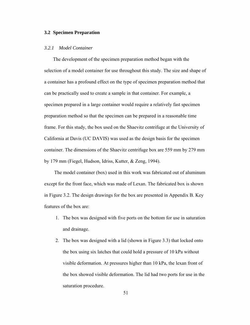
51
3.2 Specimen Preparation
3.2.1 Model Container
The development of the specimen preparation method began with the
selection of a model container for use throughout this study. The size and shape of
a container has a profound effect on the type of specimen preparation method that
can be practically used to create a sample in that container. For example, a
specimen prepared in a large container would require a relatively fast specimen
preparation method so that the specimen can be prepared in a reasonable time
frame. For this study, the box used on the Shaevitz centrifuge at the University of
California at Davis (UC DAVIS) was used as the design basis for the specimen
container. The dimensions of the Shaevitz centrifuge box are 559 mm by 279 mm
by 179 mm (Fiegel, Hudson, Idriss, Kutter, & Zeng, 1994).
The model container (box) used in this work was fabricated out of aluminum
except for the front face, which was made of Lexan. The fabricated box is shown
in Figure 3.2. The design drawings for the box are presented in Appendix B. Key
features of the box are:
1. The box was designed with five ports on the bottom for use in saturation
and drainage.
2. The box was designed with a lid (shown in Figure 3.3) that locked onto
the box using six latches that could hold a pressure of 10 kPa without
visible deformation. At pressures higher than 10 kPa, the lexan front of
the box showed visible deformation. The lid had two ports for use in the
saturation procedure.

F
F
3
sp
a
sp
m
FIG. 3.2. Mo
FIG. 3.3. Box
.2.2 Air Pl
Based on
pecimen pre
uniform voi
pecimen pre
moist spoonin
odel containe
x Lid
luviation
the literatur
paration met
id ratio and s
paration met
ng) require p
er (Box)
re review, plu
thod. Pluvia
structure thr
thods (Pluvi
post placeme
52
uviation thro
ation through
oughout the
iation throug
ent densifica
ough air was
h air may be
length of th
gh water, Dry
ation and/or l
s selected as
expected to
he sample. O
y tubing, Dr
layered spec
the
result in
Other
ry and
cimen

53
preparation to achieve the desired density. Layered preparation refers to a sample
preparation method that requires multiple layers that are first deposited and then
compacted to achieve the desired density. Post placement densification is a
process of compacting specimens (by vibration, tamping or rodding) after
placement in a mold to achieve the desired density. Both layered preparation and
post placement tamping require careful procedures and trial and error in order to
produce uniform soil deposits. Pluviation through air does not require
densification after placement or layered preparation, leading to more easily
prepared uniform specimens.
The air pluviation method implemented in this work employed a modified
version of the air pluviation/raining method used by Frost (1989). The sample
preparation apparatus shown in Figure 3.4 was developed using a plastic funnel; a
0.3 m long, 0.08 m inside diameter PVC pipe; a 5 mm opening size screen, and a
2.5 mm opening size screen. The sample preparation apparatus was based on the
pluviation apparatus fabricated by Frost (1989), and is also similar to the
apparatus used at UC Davis. The two screens were securely placed at one end of
the PVC pipe spaced at approximately 12 mm apart, with the coarser screen on
top of the finer screen. The screens were held in place by thin wires weaved
through the screens and fastened securely to the pipe through small diameter holes
drilled in the pipe. The plastic funnel was attached using duct tape at the end of
the pipe opposite to the screens to act as a receptacle for the sand.
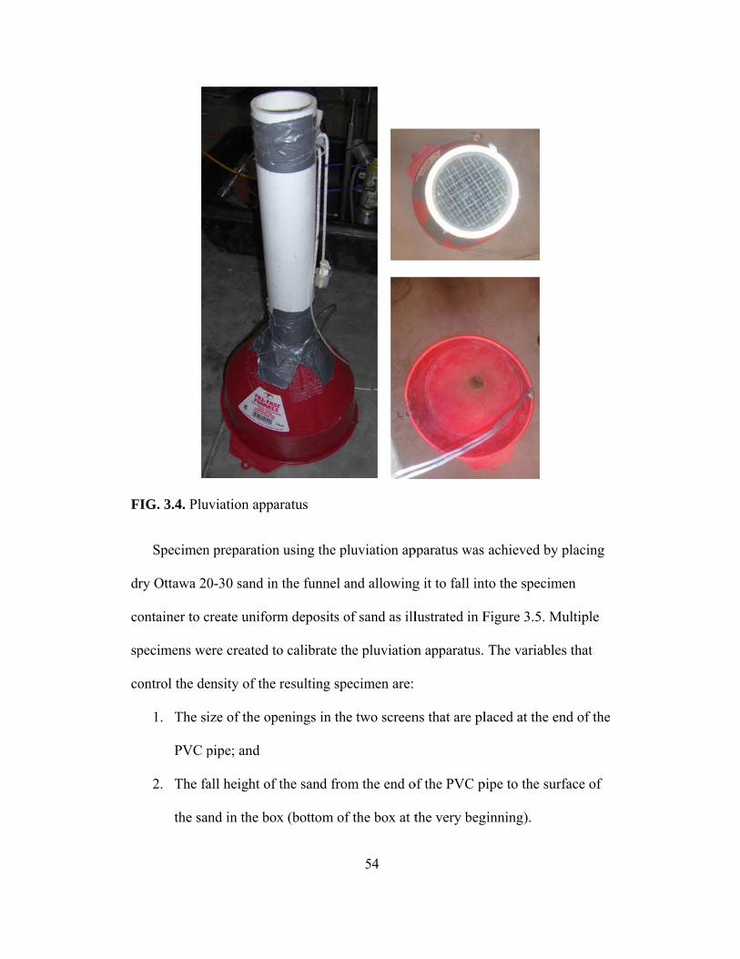
F
dr
co
sp
co
FIG. 3.4. Plu
Specimen
ry Ottawa 20
ontainer to c
pecimens we
ontrol the de
1. The si
PVC p
2. The fa
the sa
uviation appa
n preparation
0-30 sand in
create unifor
ere created to
ensity of the
ize of the op
pipe; and
all height of
and in the box
aratus
n using the p
n the funnel a
rm deposits o
o calibrate th
resulting sp
penings in th
the sand fro
x (bottom of
54
pluviation ap
and allowing
of sand as ill
he pluviation
pecimen are:
e two screen
om the end o
f the box at t
pparatus was
g it to fall int
lustrated in F
n apparatus.
ns that are pl
of the PVC p
the very beg
achieved by
nto the specim
Figure 3.5. M
The variabl
laced at the e
pipe to the su
ginning).
y placing
men
Multiple
les that
end of the
urface of
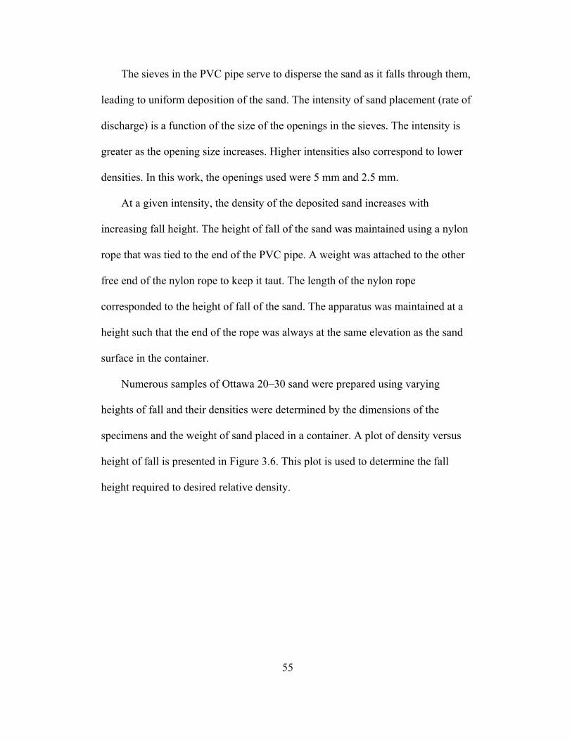
55
The sieves in the PVC pipe serve to disperse the sand as it falls through them,
leading to uniform deposition of the sand. The intensity of sand placement (rate of
discharge) is a function of the size of the openings in the sieves. The intensity is
greater as the opening size increases. Higher intensities also correspond to lower
densities. In this work, the openings used were 5 mm and 2.5 mm.
At a given intensity, the density of the deposited sand increases with
increasing fall height. The height of fall of the sand was maintained using a nylon
rope that was tied to the end of the PVC pipe. A weight was attached to the other
free end of the nylon rope to keep it taut. The length of the nylon rope
corresponded to the height of fall of the sand. The apparatus was maintained at a
height such that the end of the rope was always at the same elevation as the sand
surface in the container.
Numerous samples of Ottawa 20–30 sand were prepared using varying
heights of fall and their densities were determined by the dimensions of the
specimens and the weight of sand placed in a container. A plot of density versus
height of fall is presented in Figure 3.6. This plot is used to determine the fall
height required to desired relative density.
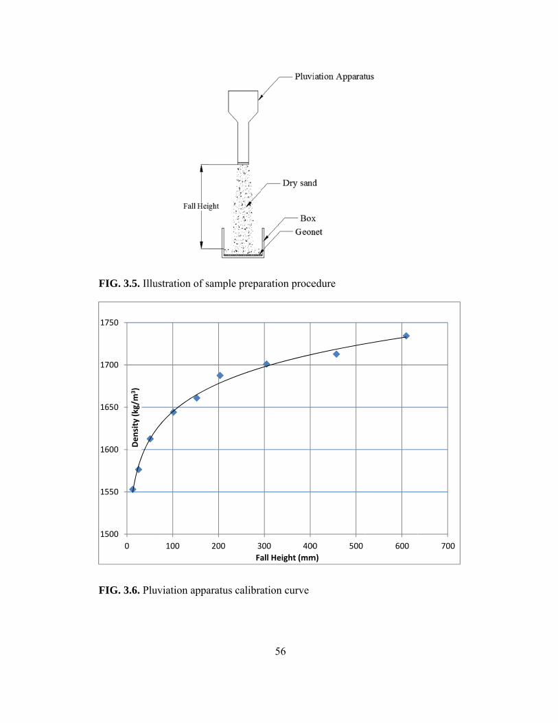
F
F
1
1
1
1
1
1
FIG. 3.5. Illu
FIG. 3.6. Plu
500
550
600
650
700
750
0
Density (kg/m
3)
ustration of s
uviation appa
100
sample prepa
aratus calibra
200 3
Fa
56
aration proce
ation curve
300 400
all Height (mm
edure
0 500
m)
600
700
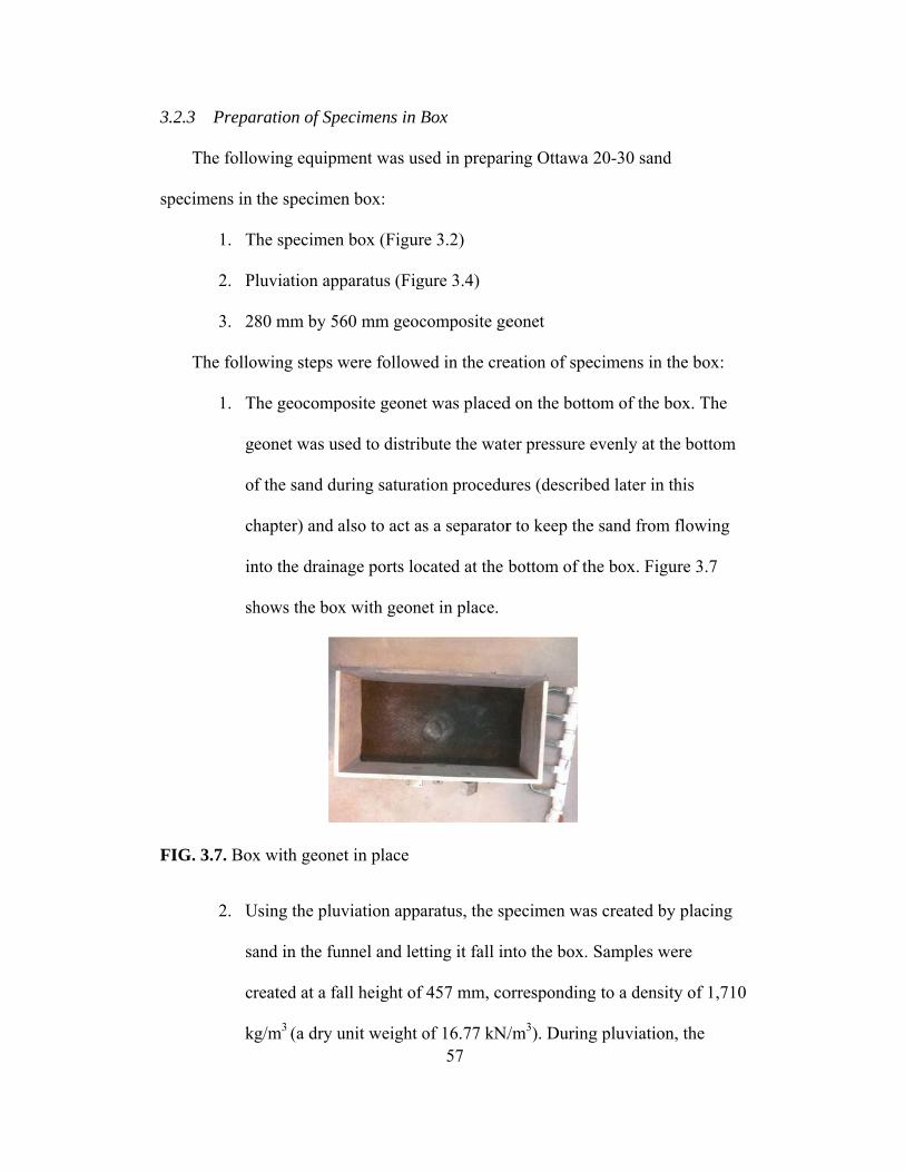
3
sp
F
.2.3 Prepa
The follo
pecimens in
1. T
2. P
3. 2
The follo
1. T
g
o
ch
in
sh
FIG. 3.7. Box
2. U
sa
cr
k
aration of Sp
owing equipm
the specime
The specimen
Pluviation ap
80 mm by 5
owing steps w
The geocomp
eonet was us
f the sand du
hapter) and a
nto the drain
hows the box
x with geone
Using the plu
and in the fu
reated at a fa
g/m3 (a dry u
pecimens in B
ment was us
en box:
n box (Figur
paratus (Fig
60 mm geoc
were followe
posite geonet
sed to distrib
uring saturat
also to act as
nage ports loc
x with geone
et in place
uviation appa
unnel and let
all height of
unit weight o 57
Box
sed in prepar
re 3.2)
gure 3.4)
composite ge
ed in the cre
t was placed
bute the wat
tion procedu
s a separator
cated at the b
et in place.
aratus, the sp
tting it fall in
f 457 mm, co
of 16.77 kN/
ring Ottawa
eonet
eation of spe
d on the botto
er pressure e
ures (describ
r to keep the
bottom of th
pecimen was
nto the box.
orresponding
/m3). During
20-30 sand
ecimens in th
om of the bo
evenly at the
ed later in th
e sand from f
he box. Figur
s created by
Samples we
g to a density
g pluviation,
he box:
ox. The
e bottom
his
flowing
re 3.7
placing
ere
y of 1,710
, the

F
3
sp
w
sa
to
T
w
sa
w
sa
d
FIG. 3.8. Plu
.2.4 Prepa
The follo
pecimens for
1. A spl
speci
memb
2. Two
3. One 7
mm.
weight tied to
and in the m
o maintain th
The pluviatio
while sand w
ample creati
weight maint
ample. The
esired heigh
uviation in pr
aration of Sp
owing equipm
r triaxial test
lit vacuum m
imens. The s
brane to allo
71 mm diam
71 mm diam
o the nylon r
model (bottom
he fall heigh
on apparatus
as continuou
ion step is sh
ained just ab
pluviation a
ht of sand wa
rogress and a
pecimens for
ment was us
ting of never
mold used fo
split vacuum
ow for pluvia
meter porous
meter confini
58
rope was ma
m of the cont
ht throughout
was raised t
usly poured
hown in Figu
bove the spe
apparatus wa
as reached.
a completed
Triaxial Tes
sed in the cre
r frozen sand
r preparation
m mold was u
ation of sand
s stones.
ng membran
aintained just
tainer at the
t the sample
to maintain t
into the funn
ure 3.8. Figu
cimen surfac
as moved bac
d specimen
sts
eation of 71
d:
n of the 71 m
used for stret
d into the co
ne with a thi
t above the t
beginning)
creation pro
the height of
nel. A pictur
ure 3.8 also s
ce and a com
ck and forth
mm diamete
mm diameter
tching the co
onfining mem
ckness of 3.
top of the
as a way
ocess.
f fall
re of this
shows the
mpleted
h until the
er
r
onfining
mbrane.
0 x 10-1

59
4. The pluviation apparatus.
5. At least two rubber O-rings
6. One source of vacuum.
The GCTS Cyclic Pneumatic Soil Triaxial System STX-050 (GCTS Testing
Systems, 2005) in the Enamul and Mahmuda Hoque Geotechnical Laboratory was
used for all triaxial tests. The following steps were employed in the creation of
specimens for triaxial testing:
1. The top assembly of the GCTS triaxial cell was removed for easier access
and to allow for pluviation of sand into the split mold. After the specimen
was created, the top assembly was replaced.
2. The confining membrane was placed over the bottom pedestal of the
triaxial cell and secured with at least one O-ring.
3. A porous stone was placed inside the confining membrane, on top of the
bottom pedestal of the triaxial cell.
4. The vacuum split mold was placed securely on the bottom pedestal with
the confining membrane inside and then the free top end of the membrane
was folded over the vacuum split mold. A vacuum was applied to the split
mold to hold the confining membrane taut against inside of the mold.
5. Using the pluviation apparatus, the specimen was created by placing sand
in the funnel and letting it fall into the confining membrane supported by
the vacuum split mold until a specimen height of at least 0.142 m was
achieved. Samples were created using a fall height of 457 mm and a

F
corre
speci
6. The s
top p
rolled
7. A co
speci
With
down
in Fig
FIG. 3.9. Tria
esponding de
imens.
second porou
laten was pl
d over the to
nfining pres
imen through
h the sample
n and the spl
gure 3.9. Ste
axial test spe
ensity of 1,7
us stone was
laced on top
op platen and
sure of 10 k
h the top pla
confined, th
lit mold was
eps 4 through
ecimen prep
60
10 kg/m3, co
s then placed
of the porou
d secured wit
kPa was then
aten drainage
he vacuum on
removed. S
h step 7 are
paration Step
onsistent wit
d on the top
us stone, and
th at least on
n applied via
e line of the
n the split va
Steps 1 throu
shown in Fi
ps 1- 4
th the box m
of the specim
d the membr
ne O-ring.
vacuum to t
GCTS triax
acuum mold
ugh step 4 are
gure 3.10.
model
men, the
rane was
the
ial cell.
d was shut
e shown

F
3
sa
sa
T
is
pr
FIG. 3.10. Tr
8. The t
top a
.2.5 Box Sp
The satur
aturation me
aturation pro
1. A sou
2. A vac
3. A sou
The samp
The initial sta
s capable of
rocedure:
1. The li
2. Air w
to the
riaxial test sp
top assembly
ssembly in p
Specimen Sat
ration proced
ethod describ
ocedure used
urce of deair
cuum source
urce of carbo
ple preparati
ate of the spe
holding a va
id was placed
as removed
box. The va
pecimen pre
y of the GCT
place, the spe
turation Pro
dure used in
bed by Ueno
d in this work
red water
e
on dioxide (C
ion method w
ecimen is dry
acuum). The
d on the box
from the san
acuum was a
61
eparation Ste
TS triaxial ce
ecimen prep
cedure
n this work w
o (2000). The
k includes:
CO2)
was describe
y Ottawa 20
saturation p
x and securel
nd specimen
applied throu
eps 1- 7
ell was then
paration was
was modeled
e equipment
ed in Section
0-30 sand in
process empl
ly fastened u
n by applying
ugh the top p
replaced. W
complete.
d after the va
t used for the
n 3.1.3 and S
the model b
loyed the fol
using the six
g a vacuum o
port of the bo
With the
acuum
e
Section.
ox which
llowing
x latches.
of 10 kPa
ox.
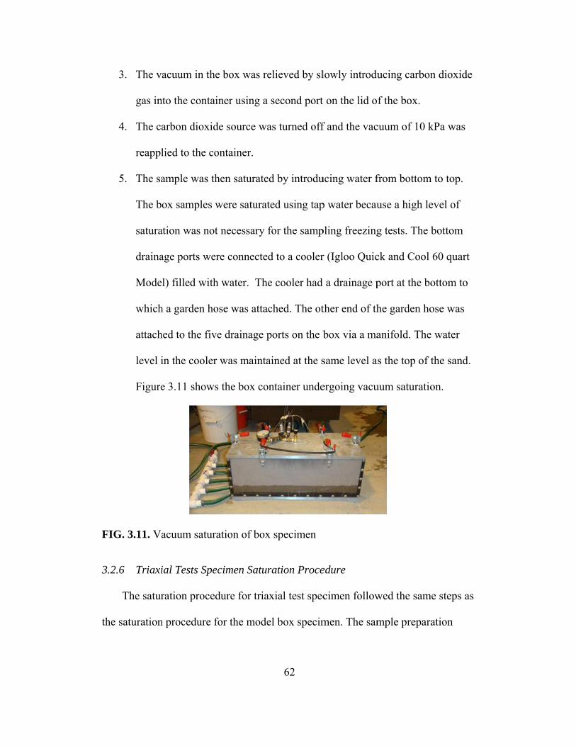
F
3
th
3. The v
gas in
4. The ca
reappl
5. The sa
The b
satura
draina
Mode
which
attach
level i
Figure
FIG. 3.11. Va
.2.6 Triaxi
The satur
he saturation
acuum in the
nto the contai
arbon dioxid
lied to the co
ample was th
ox samples w
ation was not
age ports we
l) filled with
h a garden ho
hed to the fiv
in the cooler
e 3.11 shows
acuum satur
ial Tests Spe
ration proced
n procedure f
e box was re
iner using a
de source wa
ontainer.
hen saturated
were saturat
t necessary f
ere connected
h water. The
ose was attac
ve drainage p
r was mainta
s the box con
ration of box
ecimen Satur
dure for triax
for the mode
62
elieved by sl
second port
as turned off
d by introdu
ted using tap
for the samp
d to a cooler
e cooler had
ched. The ot
ports on the b
ained at the s
ntainer unde
x specimen
ration Proce
xial test spec
el box specim
lowly introdu
t on the lid o
f and the vac
ucing water f
p water becau
pling freezing
r (Igloo Quic
a drainage p
ther end of th
box via a ma
same level a
ergoing vacu
edure
cimen follow
men. The sam
ucing carbon
f the box.
cuum of 10 k
from bottom
use a high le
g tests. The b
ck and Cool
port at the bo
he garden ho
anifold. The
as the top of t
uum saturatio
wed the sam
mple prepara
n dioxide
kPa was
m to top.
evel of
bottom
60 quart
ottom to
ose was
e water
the sand.
on.
me steps as
ation

63
method was described in section 3.2.4. The saturation procedure that was used to
saturate the triaxial test specimens is described below:
1. The specimen was placed inside a triaxial cell in order to change the
application of the confining pressure from vacuum to cell pressure.
Therefore, before the vacuum was released, a cell pressure of 10 kPa was
applied to the sample using the GCTS system from the bottom drainage
line of the cell (the cell was filled with water prior to application of the 10
kPa confining pressure). A confining pressure has to be applied to the
specimen at all times during the sample preparation and saturation
process. Otherwise, the specimen will slump over.
2. The vacuum in the specimen was relieved by slowly introducing carbon
dioxide gas into the specimen through the drainage line of the bottom cap.
3. The carbon dioxide source was turned off and the vacuum of 10 kPa was
reapplied to the sample using the top cap drainage line.
4. The sample was then hydrated, under vacuum from bottom to top using
deaired water. The vacuum and deaired water were turned off when the
sample was fully hydrated as indicated by the appearance of water in the
vacuum line.
5. Saturation was then achieved using back pressure procedure described
subsequently.

64
Chapter 4
4.0 SAMPLING PROCEDURE
4.1 Selection of Sampling Method
Based on the project constraints, the following criteria were established for the
required sampling method:
1. The method should be able to recover samples in a manner that retains
their micro structure and stress-strain behavior.
2. Since the project is a collaborative effort between three different
universities, it was important that the method be simple enough to be
reproducible by different research groups with little difficulty.
3. The method also needed to be adaptable to different model containers,
including the types used at the University of California at Davis (UC
Davis) centrifuge and State University of New York at Buffalo shake
table.
4. Sampling should be able to be performed in a relatively short time so as
not to tie up any equipment for extended periods of time.
5. The sampling method should be non-destructive to the model container.
After establishing the criteria for the required sampling method, a systematic
evaluation of the sampling methods reviewed in the literature was conducted. The
three sampling methods were evaluated on the basis of the above mentioned
criteria.
65
4.1.1 Biopolymers Agar and Agarose
The agar and agarose processes are similar in implementation. For the
purposes of technology evaluation, the agar and agarose processes were
considered under the same title of biopolymer. The following challenges were
identified with the biopolymer process:
1. From the literature review, Schneider et al. (1989)’s laboratory experiments
match closely with this study’s initial condition of the soil. Schneider et al.
(1995) used tubes inserted in the cohesionless soil for installation of:
electrodes for heating the soil; thermometers for temperature monitoring; and
an injection tube for injection of biopolymer. All these tubes are necessary for
successful impregnation with biopolymer. Experiments performed by Yoshimi
et al. (1978) show the extent of disturbance that results from pushing a tube
into cohesionless soil. Yoshimi et al. (1978) showed that a placement of a tube
in cohesionless sand results in disturbance over a distance approximately
equal to the diameter of the tube. This study may require sampling from small
containers with limited exposed surface area. Cohesionless samples would
have to be obtained at distances sufficiently far enough from all tubes to be
free of disturbance. The placement of the required tubes would effectively
reduce the number of samples that can be obtained from a physical model.
2. The biopolymer process requires heating the soil to a certain minimum
temperature prior to impregnation. Temperature monitoring is required in
order to keep the soil temperature above the gelation temperature of the
biopolymer and below the boiling temperature of water. The process of
66
heating the soil also presents an opportunity for disturbance. The possibility of
boiling the pore water is a problem that we wished to avoid. Mitchell et al.
(2005) suggests that drained heating would not result in significant volume
change and by extension, significant disturbance. However, it is a possibility
that some undrained heating might occur during heating the soil for purposes
of impregnation with biopolymer, This was also identified as a potential
source of disturbance.
3. Schneider (1989) and Sutterer et al. (1995) used the agarose impregnation and
flushing devise to remove the biopolymer from samples prior to testing. There
is not information on other biopolymer removal processes that do not rely on
the use of the impregnation and flushing device. The biopolymer
impregnation and flushing device was specifically designed for triaxial test
specimens. This did not suit the selection criteria because it requires
fabrication of a special device for biopolymer removal. Triaxial compression
tests are planned for the recovered undisturbed samples. The use of a special
fabricated device to remove biopolymer from triaxial specimens meant that
additional devices would be needed for subsequent tests.
4. Complete removal of the biopolymer is difficult to achieve.
For the reasons outlined above, the biopolymer process was judged not to be
simple enough to be seamlessly transferable and reproducible at different
universities. The biopolymer process also provided multiple opportunities for
introducing disturbance in the samples.
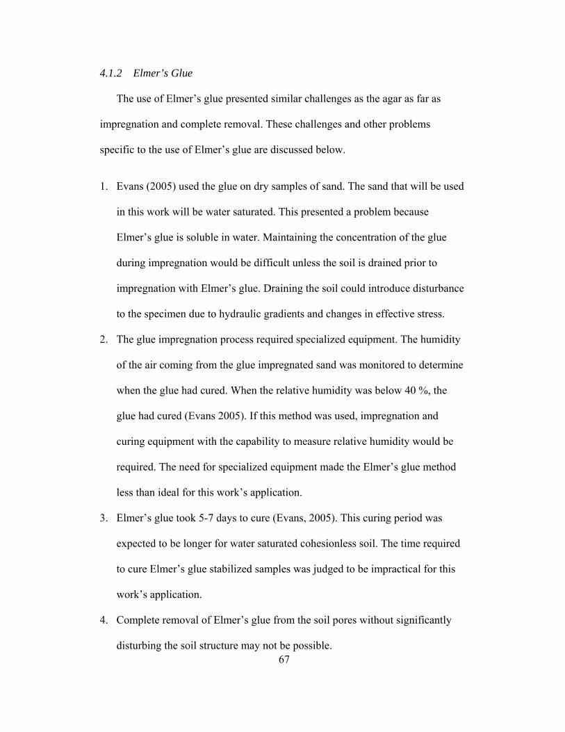
67
4.1.2 Elmer’s Glue
The use of Elmer’s glue presented similar challenges as the agar as far as
impregnation and complete removal. These challenges and other problems
specific to the use of Elmer’s glue are discussed below.
1. Evans (2005) used the glue on dry samples of sand. The sand that will be used
in this work will be water saturated. This presented a problem because
Elmer’s glue is soluble in water. Maintaining the concentration of the glue
during impregnation would be difficult unless the soil is drained prior to
impregnation with Elmer’s glue. Draining the soil could introduce disturbance
to the specimen due to hydraulic gradients and changes in effective stress.
2. The glue impregnation process required specialized equipment. The humidity
of the air coming from the glue impregnated sand was monitored to determine
when the glue had cured. When the relative humidity was below 40 %, the
glue had cured (Evans 2005). If this method was used, impregnation and
curing equipment with the capability to measure relative humidity would be
required. The need for specialized equipment made the Elmer’s glue method
less than ideal for this work’s application.
3. Elmer’s glue took 5-7 days to cure (Evans, 2005). This curing period was
expected to be longer for water saturated cohesionless soil. The time required
to cure Elmer’s glue stabilized samples was judged to be impractical for this
work’s application.
4. Complete removal of Elmer’s glue from the soil pores without significantly
disturbing the soil structure may not be possible.
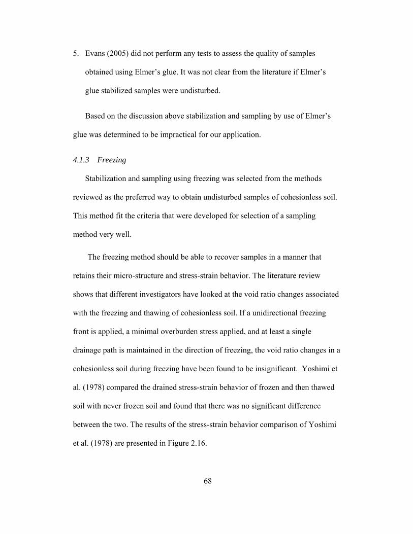
68
5. Evans (2005) did not perform any tests to assess the quality of samples
obtained using Elmer’s glue. It was not clear from the literature if Elmer’s
glue stabilized samples were undisturbed.
Based on the discussion above stabilization and sampling by use of Elmer’s
glue was determined to be impractical for our application.
4.1.3 Freezing
Stabilization and sampling using freezing was selected from the methods
reviewed as the preferred way to obtain undisturbed samples of cohesionless soil.
This method fit the criteria that were developed for selection of a sampling
method very well.
The freezing method should be able to recover samples in a manner that
retains their micro-structure and stress-strain behavior. The literature review
shows that different investigators have looked at the void ratio changes associated
with the freezing and thawing of cohesionless soil. If a unidirectional freezing
front is applied, a minimal overburden stress applied, and at least a single
drainage path is maintained in the direction of freezing, the void ratio changes in a
cohesionless soil during freezing have been found to be insignificant. Yoshimi et
al. (1978) compared the drained stress-strain behavior of frozen and then thawed
soil with never frozen soil and found that there was no significant difference
between the two. The results of the stress-strain behavior comparison of Yoshimi
et al. (1978) are presented in Figure 2.16.

69
The laboratory freezing process used by Yoshimi et al. (1978) to investigate
the volume changes due to freezing (shown in Figure 2.10) appeared simple
enough to be easily replicated and is therefore the basis of the freezing process
that was developed for this study. Since the project is a collaborative effort
between three different universities, it was important that the method be simple
enough to be reproducible by different researchers with little difficulty. The
freezing process does not require insertion of anything into the soil. The soil is
frozen by application of a cold front at the surface of the model. Yoshimi et al.
(1978) applied the freezing surface at the bottom of the soil.
Freezing is adaptable to different model containers. Since the freezing front
is applied at the surface of the container, the freezing application contact area can
be increased or reduced to suit the size of model container and thus, is adaptable
to different size containers. This adaptability is important because the freezing
method will be used at both the University of California at Davis (UC Davis)
centrifuge and State University of New York at Buffalo shake table in this
research program.
4.2 Development of Freezing Procedure
Following the selection of freezing as the stabilization method, a plan for
development of a freezing method was initiated. The objective of the plan was to
develop a method to freeze uniform specimens of sand by applying a
unidirectional freezing front while maintaining at least one drainage path in the
direction of freezing front propagation.

70
4.2.1 Freezing Procedure
As mentioned above, the objective of the work described herein was to
develop a method for undisturbed sampling of cohesionless soil within the
laboratory environment. The freezing procedure was developed for the box model
container that was described earlier. The freezing procedure was modeled after
the bottom up laboratory procedure that was used by Yoshimi et al., (1978). The
following equipment/materials were required for freezing and sampling the soil in
the model box:
1. A metal pan with a flat bottom. A baking pan 254 mm by 508 mm by
25.4 mm was used in our freezing tests.
2. Ethanol. Koptec 200 proof ethanol was used in all freezing tests
3. Dry ice
The freezing procedure consisted of the following steps:
1. The initial state of the specimen to be frozen was the saturated sand in the
box connected to a cooler full of water with no head difference between
the cooler and the box. The first step was to establish a drainage path for
water expelled from the box. This was achieved by making sure that the
connection between the box and cooler was open.
2. Dry ice was placed into the pan, the pan containing dry ice was then
carefully placed on top of the saturated sand in intimate contact with the
sand, and the alcohol was slowly poured into the pan using a funnel.

71
3. The dry ice was replenished as it was used up while monitoring the
progress of the freezing. Freezing progress was monitored through the
lexan panel that formed one side of the box.
4. When the required thickness of sand was frozen, the freezing process was
stopped by removing the pan filled with the mixture of alcohol and dry
ice from the specimen. The pan had a tendency to stick to the surface of
the sand. A little tapping was required to free the pan from the frozen
sand. The time it takes to freeze the sample is a function of, among other
things, the quantity of sand to be frozen, the ambient temperature, and the
material to be frozen. Freezing the entire mass of sand caused the sand to
stick to the geonet and interfere with the sample recovery. To avoid this,
the sand was only frozen to approximately 25 mm from the bottom, as
observed through the lexan side of the box. It took approximately 2.5 to
3.5 hours to freeze the sand in the box to a depth of approximately 150
mm.
4.2.2 Numerical Modeling of Freezing Front Propagation
The literature review indicated that during freezing of water saturated sand,
pore water migrates in the liquid phase to accommodate the expansion of the pore
water as it freezes. A uni-directional freezing front is desired such that no liquid
water is trapped due to impeded drainage by either frozen sand or an impermeable
surface. If other freezing fronts developed at the bottom or sides of the box, e.g.
due to potential freezing temperatures along the metal sides of the container, then
the freezing front would not be uni directional. Multiple freezing fronts in the box

m
tw
es
fr
th
th
lo
al
F
ai
m
F
fr
al
might trap liq
wo dimensio
stablish that
reezing setup
The finit
he freezing m
he short (279
ogically, the
long the met
igure 4.1. Th
ir on both sid
method.
FIG. 4.1. Ske
The box
ront is made
luminum wi
quid water le
onal finite ele
a unidirectio
p.
e element pr
method. A tw
9 mm (11 inc
critical cros
tal sides of th
he numerica
des and fina
etch of nume
was conserv
of lexan). T
th inside dim
eading to dist
ement nume
onal freezing
rogram SVH
wo-dimensio
ches)) dimen
ss section wi
he box. A sk
al model show
ally, coolant t
erical model
vatively mod
The geometry
mensions of
72
turbance of
erical analysi
g front was i
Heat (Soil Vi
onal steady s
nsion of the
ith respect to
ketch of the
ws the alum
to top consis
deled to be m
y of the box
280 mm by
the soil struc
is of heat flo
induced in th
ision, 2010)
state analysis
box, as the s
o heat flow (
SVHeat mod
minum box bo
stent with th
made entirely
was as built
180 mm. La
cture. There
ow were con
he model du
was used to
s was conduc
short dimens
or cold) tran
del is shown
ounded by la
he described
y of aluminu
t, 13 mm thi
ayers of air w
efore, a
nducted to
uring the
model
cted in
sion was
nsfer
n in
ayers of
freezing
um (the
ck
were

d
T
te
b
b
w
cr
re
F
efined aroun
The outside b
emperature).
e -68°C. Thi
ottom of the
The resu
would propag
reating secon
esults of the
FIG. 4.2. Num
nd the alumin
boundaries o
We measur
is is similar
e model was
lt of the finit
gate from the
ndary freezin
numerical m
merical Mod
num box to
f the air laye
red the tempe
to the tempe
modeled as
te element in
e coolant sur
ng fronts fro
modeling.
deling of Fre
73
simulate lab
ers had a con
erature of th
erature repor
constant flu
nvestigation
rface down t
om the sides
eezing Front
boratory boun
nstant tempe
he alcohol an
rted by Yosh
ux boundary.
showed tha
to the bottom
of the box.
t Propagation
undary condit
erature of 80
nd dry ice mi
himi et al (19
.
at freezing fr
m of the box
Figure 4.2 s
n
tions.
0°F (room
ixture to
978). The
ont
x without
hows the

4
pr
sa
p
sa
fo
p
th
in
th
w
th
.2.3 Exper
Labor
ropagation o
and in the m
laced in the
and by pluvi
orm that was
lace during p
hermocouple
nvestigated b
hermocouple
was expected
hermocouple
rimental Inve
ratory experi
of the freezin
model box as
model at pre
iation. The th
s fabricated f
pluviation. S
es are shown
because, as n
es were place
d to be symm
es were num
estigation of
iments were
ng front. Fre
described ab
edetermined
hermocouple
for this expe
Sketches of t
n in Figure 4
noted before
ed in only ha
metrical abou
mbered as sho
74
f Freezing Fr
also conduc
eezing experi
bove except
d different loc
es were plac
eriment to se
the form and
.3. Only the
, it is the mo
alf of the cro
ut the middle
own in Figur
(a)
Front Propag
cted to inves
iments were
that eight th
cations prior
ced in the mo
ecurely hold
d the location
short dimen
ost critical di
oss section b
e plane of the
re 4.3.
gation
stigate the
e setup by pla
hermocouple
r to placeme
odel using a
the thermoc
ns of the
nsion (280 m
imension. Th
because the f
e box. The
acing
es were
ent of
wooden
couples in
mm) was
he
freezing
F
th
re
T
co
d
T
fr
T
co
d
fr
bu
ex
FIG. 4.3. Fre
After satu
he coolant on
ecord the tem
The trend of t
oincide with
The resu
irectionally
Thermocoupl
reezing temp
Thermocoupl
ontainer, the
id. Followin
rozen soil wa
ulb of the fro
xcavated fro
eezing front i
uration, free
n top of the s
mperature of
temperature
h the thermom
lts of the exp
to the same
le 1 was the
perature. Th
le 5. If a seco
ermocouples
ng completio
as excavated
ozen soil als
ozen bulb is s
investigation
ezing was ini
saturated san
f the sand at
drop was no
meters recor
periments sh
configuratio
first to freez
hermocouple
ondary freez
2, 5 and 8 w
on of the free
d to inspect t
so confirmed
shown in Fig
75
(b)
n experimen
itiated by pla
nd. The therm
the location
oted and the
rding a temp
howed that th
on as predict
ze and therm
e 4 recorded
zing front de
would have f
ezing front p
the shape of
d the numeri
gure 4.4.
ntal setup
acing the me
mocouples w
ns shown in F
onset of free
perature of 0°
he freezing f
ted by the nu
mocouple 8 w
a freezing te
eveloped alon
frozen much
propagation i
f the frozen s
cal analysis
etal pan cont
were monito
Figure 4.3 w
ezing was as
° C.
front propag
umerical ana
was last to re
emperature b
ng the sides
h sooner than
investigation
soil. The sha
result. The
taining
ored to
with time.
ssumed to
gated uni-
alyses.
ecord a
before
of the
n they
n, the
ape of the

F
se
sh
co
st
4
p
du
fr
un
te
to
pr
FIG. 4.4. For
The therm
ection 4.2.1
hape of the f
onsistent wit
teady state n
.2.4 Expan
Yoshimi
ath, and surc
ue to freezin
rozen multip
nder the con
As discu
echnique des
op to bottom
rocess. Base
rm with therm
mocouple ex
induced a un
frozen soil ex
th the conclu
numerical an
nsion of Satu
et al. (1978)
charge were
ng of pore w
ple times in o
nditions desc
ssed in the p
scribed in se
m. The draina
ed on observ
mometers an
xperiment sh
nidirectional
xcavated aft
usions reach
alysis.
urated Soil d
) concluded
necessary to
ater. Ottawa
order to inve
cribed in Sec
previous sect
ction 3.3 res
age path was
vations made
76
nd frozen bu
howed that th
l freezing fro
ter the exper
hed from the
during Freez
that a unidir
o limit the di
a 20-30 sand
estigate the e
ction 4.2.1.
tion, it was c
sulted in a un
s also kept op
e during mult
ulb of sand
he freezing m
ont to the sat
rimental inve
temperature
zing
rectional fre
isturbance o
d specimens i
expansion du
confirmed th
nidirectional
pen througho
tiple freezin
method desc
turated soil.
estigation wa
e measureme
ezing front,
of the cohesio
in the box w
ue to freezin
hat the freezi
l freezing fro
out the freez
ng trials, it w
cribed in
The
as
ent data
drainage
onless
were
g soil
ing
ont from
zing
was
co
kP
o
b
ou
th
n
F
fr
F
4
fr
te
sp
o
d
oncluded tha
Pa) was ade
f the frozen
ox to accom
ut over the e
he theory tha
ine percent e
igure 4.5 sho
ront propaga
FIG. 4.5. Wa
.3 Developm
Followin
rozen sample
esting 35mm
pecialized pl
f 35 mm dia
iameter sam
at the surcha
quate to lim
soil would r
mmodate the
edge of the m
at water is ex
expansion of
ows water fl
ated.
ater flowing
ment of Cor
ng the develo
es was also d
m diameter an
latens. Samp
ameter sampl
mples were go
arge due to th
it expansion
result in heav
expansion. W
model box, d
xpelled in fro
f water when
lowing over
out of box d
ring Techni
opment of a
developed. M
nd 71 mm di
ples required
les. For thes
oing to be re
77
he weight of
n to negligibl
ving of the s
Water in liqu
during freezi
ont of the fre
n it changes
the edge of
during freezin
ique
freezing tech
Most triaxial
iameter test
d for microst
e reasons, it
ecovered for
f the pan fille
le levels. Sig
soil surface o
uid phase wa
ng experime
eezing front
phase from
the model b
ng
hnique, a me
l testing syst
samples wit
tructure stud
t was decided
testing.
ed with cool
gnificant exp
or deformati
as observed
ents, consiste
to accommo
liquid to sol
box as the fre
ethod to reco
tems are cap
thout requirin
dies are on th
d initially th
lant (0.8
pansion
on of the
flowing
ent with
odate the
lid.
eezing
over
pable of
ng
he scale
hat 35mm
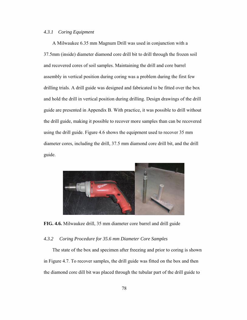
4
3
an
as
dr
an
gu
th
u
d
gu
F
4
in
th
.3.1 Corin
A Milwa
7.5mm (insi
nd recovered
ssembly in v
rilling trials.
nd hold the d
uide are pres
he drill guide
sing the dril
iameter core
uide.
FIG. 4.6. Mil
.3.2 Corin
The state
n Figure 4.7.
he diamond c
g Equipmen
aukee 6.35 m
ide) diameter
d cores of so
vertical posit
. A drill guid
drill in vertic
sented in Ap
e, making it
l guide. Figu
es, including
lwaukee dril
ng Procedur
e of the box a
. To recover
core dill bit
nt
mm Magnum
r diamond co
oil samples. M
tion during c
de was desig
cal position
ppendix B. W
possible to r
ure 4.6 show
g the drill, 37
ll, 35 mm dia
re for 35.6 m
and specime
samples, the
was placed t
78
m Drill was u
ore drill bit t
Maintaining
coring was a
gned and fab
during drilli
With practice
recover mor
ws the equipm
7.5 mm diam
ameter core
mm Diameter
en after freez
e drill guide
through the t
used in conju
to drill throu
g the drill and
a problem du
bricated to be
ing. Design d
e, it was pos
e samples th
ment used to
mond core dr
barrel and d
r Core Samp
zing and prio
was fitted o
tubular part
unction with
ugh the froze
d core barrel
uring the firs
e fitted over
drawings of
sible to drill
han can be re
o recover 35
rill bit, and th
drill guide
ples
or to coring i
on the box an
of the drill g
a
en soil
l
st few
the box
f the drill
l without
ecovered
mm
he drill
is shown
nd then
guide to

st
ex
w
sh
te
ap
3
p
pr
b
F
F
tart drilling.
xcessive am
was removed
hows sample
echnique is s
pproximately
7.5 mm core
erimeter. Th
remature tha
een recovere
FIG. 4.7. Box
FIG. 4.8. Cor
Drilling was
ount of force
d and the froz
e recovery in
shown in Fig
y 35 mm in
e barrel was
he samples w
awing. Figur
ed from it.
x after freezi
ring in progr
s performed
e. After drill
zen cores sim
n progress. A
gure 4.8. The
diameter and
used, the rec
were stored in
re 4.9 shows
ing
ress and reco
79
by one pers
ling through
mply fell out
A typical sam
e sample sho
d 162.5 mm
covered core
n a freezer s
s the frozen m
overed 35 m
son and did n
h the frozen m
t of the drill
mple recover
own in Figur
m in length. N
e was melty
soon after rec
mass of soil
mm diameter
not require a
material, the
bit. Figure 3
red using thi
re 4.8 was
Note that alth
around the
covery to av
after sample
core
an
e drill bit
3.18
is
hough a
void
es have

F
an
4
sa
re
F
FIG. 4.9. Box
After sam
nd stored in
.3.3 Corin
For reaso
amples were
ecover 71 mm
1. 71 m
2. Shelb
the S
3. A Mi
4. Husq
5. Core
FIG. 4.10. St
x and sand a
mples were r
a freezer for
g Procedure
ons discussed
e required fo
m diameter
mm internal d
by tube drill
helby tube d
ilwaukee 6.3
qvarna DR 15
Drill Rig A
teel pipe use
after coring
recovered, th
r later retriev
e for 71 mm
d in Chapter
r triaxial tes
core sample
diameter stee
adaptor (Sh
drill adaptor
35 mm Magn
50 Core Dril
Adaptor (Sho
d for 71 mm
80
hey were pla
val and testin
Diameter co
r 5, it was de
ting. The fol
s:
el pipe (Show
hown in Figu
is presented
num Drill (se
ll Rig (Show
own in Figur
m cores
aced in a con
ng.
ore Samples
ecided that 7
llowing equi
wn in Figure
ure 4.11). Th
d in Appendi
ee Figure 4.6
wn in Figure
re 4.12)
nfining memb
71 mm diame
ipment was
e 4.10)
he design dra
ix A
6)
4.12)
mbrane
eter core
used to
awing of
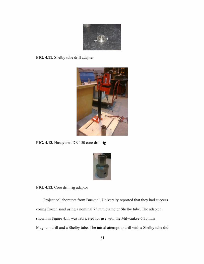
F
F
F
co
sh
M
FIG. 4.11. Sh
FIG. 4.12. Hu
FIG. 4.13. Co
Project c
oring frozen
hown in Figu
Magnum drill
helby tube dr
usqvarna DR
ore drill rig a
ollaborators
n sand using
ure 4.11 was
l and a Shelb
rill adapter
R 150 core d
adaptor
from Buckn
a nominal 7
s fabricated
by tube. The
81
drill rig
nell Universi
5 mm diame
for use with
e initial attem
ity reported
eter Shelby t
the Milwau
mpt to drill w
that they ha
tube. The ad
ukee 6.35 mm
with a Shelby
ad success
dapter
m
y tube did

n
tr
n
p
th
th
p
S
sp
p
re
d
F
O
ot work beca
ry. The decis
early circula
ipe was also
It was sig
he 37.5 mm
his regard bu
erfectly roun
helby tube w
pinning pipe
enetration w
equired to in
iameter pipe
FIG. 4.14. Co
Samples
Occasionally,
ause the She
sion was mad
ar and did no
o strong enou
gnificantly h
core barrel.
ut also wore
nd and, it wo
wobbled. Th
e on the surfa
was achieve t
nitiate and co
e is shown in
oring with 7
were readily
, the cores g
elby tube wo
de to use a m
ot wobble as
ugh to be gro
harder to star
The cutting
out as the co
obbled slight
e procedure
ace of the sa
to hold the p
ontinue drilli
n Figure 4.14
1 mm diame
y obtained af
ot stuck in th
82
obbled and d
machined ste
much as the
ound to creat
rt coring wit
teeth created
oring progre
tly during co
used to adva
and as steady
pipe in place.
ing to depth.
4.
eter steel pip
fter coring w
he pipe and
deformed the
eel pipe whic
e Shelby tub
ate cutting tee
th the 71 mm
d prior to co
essed. The pi
oring but not
ance the cor
y as possible
. Considerab
. Coring with
pe
without much
a sample ext
e adaptor on
ch was more
be during dri
eth on the pi
m steel pipe t
oring helped
ipe was near
t as much as
re was to hol
e until enoug
ble effort wa
h the 71 mm
h difficulty.
truder was u
the first
e rigid,
lling. The
ipe.
than with
a lot in
rly
s the
ld the
gh
as
m
used to

re
h
S
en
p
sa
sa
sa
m
ac
co
re
w
th
ecover the sa
ave been rec
FIG. 4.15. L
The samp
helby tube w
nough for tri
lace and ver
ample was u
amples are r
and in the bo
mm. The tape
chieve a uni
ombination o
esulted in tri
Initial co
with a steel tu
he tube that w
ample. The 7
covered from
Large 71 mm
ples recover
were general
iaxial testing
rtical at the b
usually tapere
equired to b
ox container
ered portion
form cross s
of the recove
immed samp
oring trials w
ube without
was used wi
71 mm diam
m it are show
m diameter s
red using the
lly acceptabl
g. Due to the
beginning of
ed. For triax
e at least 142
specimens r
of the recov
section of the
ered sample
ples that wer
with the Husq
any cutting t
th the Milwa
83
meter sample
wn in Figure
samples and
e Milwaukee
le except tha
e difficulty in
f coring, the t
xial testing o
2 mm in hei
ranged from
vered sample
e triaxial test
height and t
e too short f
qvarna DR 1
teeth. A stee
aukee 6.35 m
and the mod
4.15.
specimen af
e 6.35 mm M
at they were
n keeping th
top 10 to 30
f 71 mm dia
ght. The thic
m approximat
es had to be t
t sample. In
the length of
for triaxial te
150 core dril
el tube, with
mm Magnum
del box after
fter sample r
Magnum Dril
often not lon
he Shelby tub
0 mm portion
ameter samp
ckness of the
tely 150 mm
trimmed in o
certain case
f the tapered
esting.
l rig were co
a thinner wa
m Drill was f
r samples
recovery
ll and
ng
be in one
n of the
les,
e frozen
m to 165
order to
es, the
d section
onducted
all than
fabricated

fo
m
ob
d
co
d
cr
in
u
C
co
F
or use with t
minimal effor
bserved from
iameter and
oring by app
id not elimin
reate cutting
nternal diam
se of a pipe
Coring with t
oring rig are
FIG. 4.16. Co
he core drill
rt (weight of
m the initial
in certain tr
plication of p
nate the prob
g teeth in ma
eter pipe tha
with cutting
the coring rig
e shown in F
oring with co
l rig. The ste
f the assemb
trials. The sa
ials, were ta
pressure redu
blem out righ
anner similar
at was used w
g teeth elimin
g is shown in
igure 4.17
oring rig
84
eel tube cored
ly). Signific
amples reco
apered at the
uced the amo
ht. The thin
r to the cuttin
with the Mil
nated the me
n Figure 4.1
d through th
cant melting
vered, were
top. Increas
ount of melt
walled steel
ng teeth crea
lwaukee 6.35
elting and tap
6 and sampl
he frozen san
of the samp
less than 71
sing the spee
ting and tape
l tube was gr
ated on the 7
5 Magnum D
pering probl
les obtained
nd with
le was
1 mm in
ed of
ering but
round to
71 mm
Drill. The
lem.
using the

F
h
4
sa
FIG. 4.17. Sa
Followin
old plastic w
.3.4 Corin
The follo
ampling tech
1. Keep
challe
work
need
pract
guide
the in
ample Recov
ng recovery,
wrap” wrap a
ng Challenge
owing challe
hnique:
ping the 37.5
enge. The dr
ked well. How
to drill in th
ice the chall
e was overco
nclination of
vered Using
the 71 mm d
and aluminum
es
enges were e
5 mm diamon
rill guide wa
wever, when
he middle of
lenge of keep
ome; a secon
f the drill bit
85
Coring Rig
diameter sam
m foil and th
ncountered i
nd core drill
as designed t
n more samp
the box, the
ping the core
nd person wa
during drill
mples were w
hen stored in
in the develo
l bit vertical
to solve this
ples are requ
e drill guide
e drill vertic
as used to he
ling.
wrapped in ‘
n a freezer.
opment of th
during drilli
problem and
uired and the
cannot be us
cal without th
elp orient an
house
he
ing was a
d it
re is a
sed. With
he drill
nd correct

86
2. When the specimen in the box is frozen all the way to the bottom, the
samples tended to stick to the filter fabric at the bottom of the box. When
this happened, the sample stayed within the hole when the diamond core
drill bit was withdrawn. Recovery of the sample without damage was
difficult to achieve in this instance.
3. During drilling, it was important to drill nonstop. When drilling was
stopped while the diamond core drill bit was still in the hole, the material
around the diamond core bit froze making it very difficult to restart the
drill. There were times when the specimen had to be abandoned because
sampling could not be restarted after the diamond core bit got stuck.
4. Cohesion between the inside of the diamond core drill bit and the sample
sometime kept the sample trapped in the core barrel. When sample for
stuck in the core barrel, it was removed by pouring cold tap water around
the outside of the diamond core drill bit. The relatively warm tap water
melted the surface of the sample, freeing it from the diamond core drill
bit. This method of freeing the sample came at a risk of reducing the
diameter of the recovered sample by melting too much of the surface.
5. The samples were stored in a cold freezer right after recovery to mitigate
premature thawing. An easily accessible storage facility or container
capable of maintaining freezing temperatures was required.
6. Coring 71 mm samples using the Milwaukee drill and the steel pipe was
very difficult because the steel pipe used as a core barrel was not
perfectly round and tended to wobble during drilling. In the absence of a
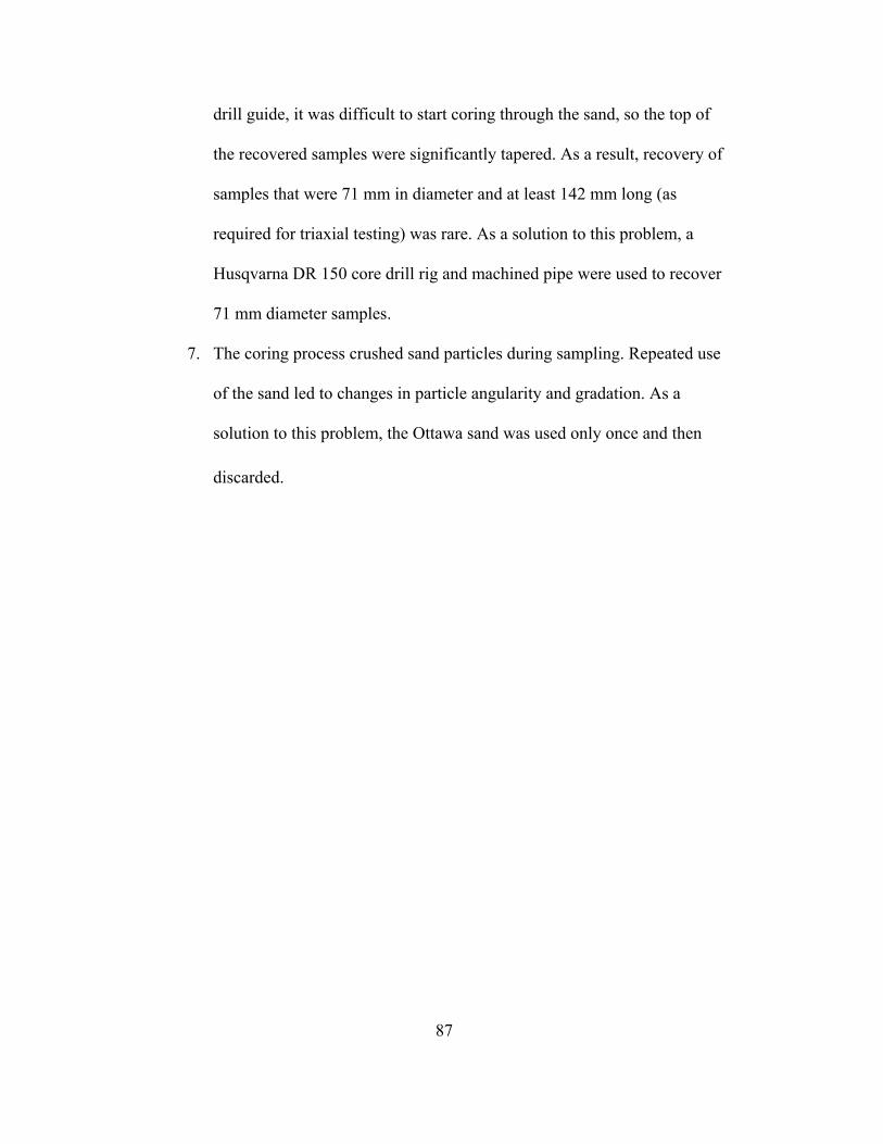
87
drill guide, it was difficult to start coring through the sand, so the top of
the recovered samples were significantly tapered. As a result, recovery of
samples that were 71 mm in diameter and at least 142 mm long (as
required for triaxial testing) was rare. As a solution to this problem, a
Husqvarna DR 150 core drill rig and machined pipe were used to recover
71 mm diameter samples.
7. The coring process crushed sand particles during sampling. Repeated use
of the sand led to changes in particle angularity and gradation. As a
solution to this problem, the Ottawa sand was used only once and then
discarded."
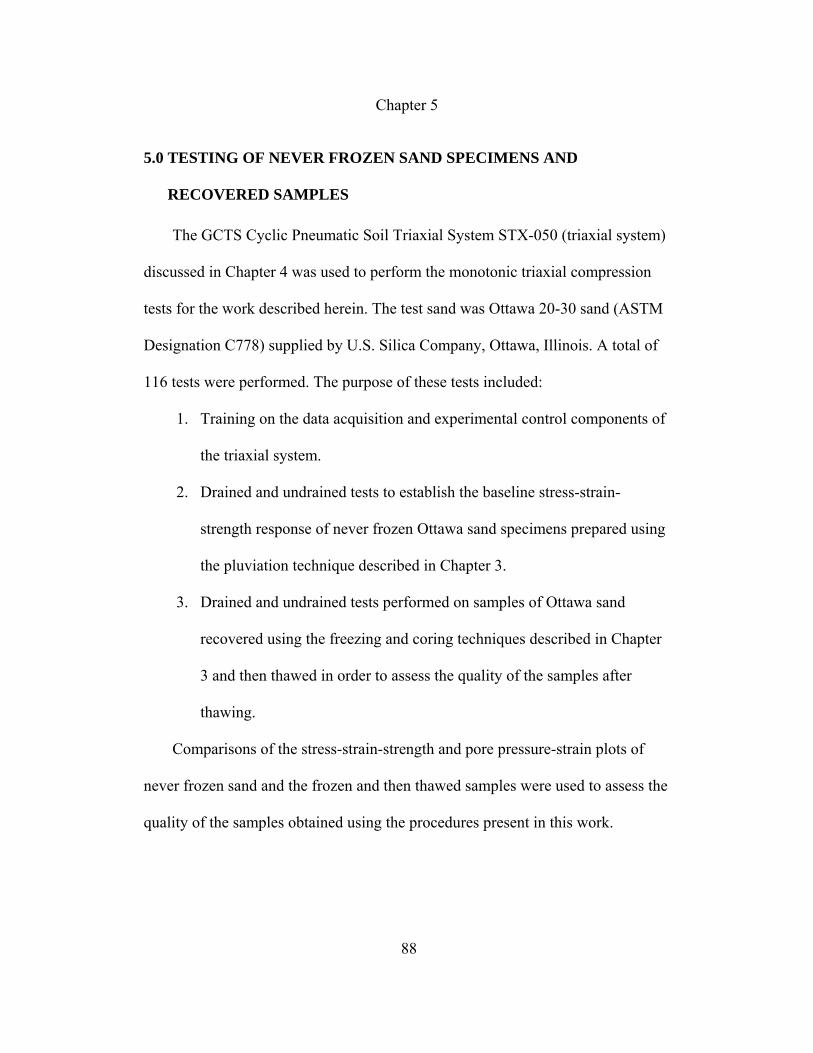
88
Chapter 5
5.0 TESTING OF NEVER FROZEN SAND SPECIMENS AND
RECOVERED SAMPLES
The GCTS Cyclic Pneumatic Soil Triaxial System STX-050 (triaxial system)
discussed in Chapter 4 was used to perform the monotonic triaxial compression
tests for the work described herein. The test sand was Ottawa 20-30 sand (ASTM
Designation C778) supplied by U.S. Silica Company, Ottawa, Illinois. A total of
116 tests were performed. The purpose of these tests included:
1. Training on the data acquisition and experimental control components of
the triaxial system.
2. Drained and undrained tests to establish the baseline stress-strain-
strength response of never frozen Ottawa sand specimens prepared using
the pluviation technique described in Chapter 3.
3. Drained and undrained tests performed on samples of Ottawa sand
recovered using the freezing and coring techniques described in Chapter
3 and then thawed in order to assess the quality of the samples after
thawing.
Comparisons of the stress-strain-strength and pore pressure-strain plots of
never frozen sand and the frozen and then thawed samples were used to assess the
quality of the samples obtained using the procedures present in this work.

89
5.1 Test Parameters
5.1.1 Initial Density
All tests specimens were prepared using the pluviation apparatus described in
Chapter 3. The fall height was maintained at 457 mm. The density of the samples
prepared at this fall height was approximately 1,710 kg/m3. Maximum and
minimum densities of Ottawa 20-30 sand were calculated as 1,764 kg/m3 and
1,521 kg/m3, respectively, using values of minimum and maximum void ratio
published by Santamatina et al. (2001), assuming zero percent saturation. Based
on the calculated maximum and minimum densities, the relative density of the
resulting specimens was 80%.
The density of each specimen prepared for this testing program was verified
using direct measurements on the prepared specimens. One method to determine
how much sand is in a specimen is to start with a known mass of sand and then
weigh the remaining sand after the sample has been created. However, pluviation
results in significant loss of sand due to scatter. Therefore, to verify the density of
the pluviated specimens, the sand in the specimen was collected after completion
of the triaxial compression tests, oven dried, and weighed.
The density of the specimen created in the box was also confirmed by
measuring the density of six cores recovered from the frozen box sample using
methods described in Chapter 4. These samples were used for density tests only,
no triaxial tests were performed on these samples. The density was determined by
measuring the volume of the frozen cores, oven drying the cores, and then

90
measuring the mass of the dry sand. The results of the density tests are presented
in Table 5-1.
Table 5-1. Density Confirmation Test Results
Core # 1 2 3 4 5 6
Density
(kg/m3) 1699 1688 1709 1696 1697 1689
5.1.2 Confining Pressure
The triaxial compression tests were conducted at an effective confining
pressure of 60 kPa. This confining pressure was chosen to be consistent with the
confining pressures employed by Bucknell University, one of our collaborating
partners on the larger project.
5.1.3 Specimen Saturation
Following vacuum hydration of the sample as described in Chapter 3, back
pressure techniques were used to saturate the specimen. Based on the relationship
between Skempton’s B-value (the ratio of the change in pore pressure to the
change in isotropic confining pressure under undrained conditions) and the degree
of saturation, a B-value of at least 0.90 was chosen as the indicator of saturation,
i.e. of the point at which the triaxial tests could be performed. As illustrated in
Figure 5.1, the level of saturation for Ottawa sand is nearly 100 percent when the
B-value (pore pressure parameter, B) is 0.9. This standard was applied to both
drained and undrained tests.

F
co
un
T
th
pr
B
co
co
b
un
ac
FIG. 5.1. B-v
For the i
onfined unde
nder the load
The B-value w
he drainage l
ressure. The
B-value was l
onfining pre
onfining pre
ack pressure
ntil a B-valu
chieved at b
value as a fun
initial step in
er an effectiv
d cell and a n
was determi
lines closed
e drainage lin
less than 0.9
essure was al
essure of 20 k
e by repeatin
ue greater tha
ack pressure
nction of de
n back pressu
ve pressure o
nominal sea
ned by incre
and recordin
nes were reo
9, the back pr
lso increased
kPa. A new
ng the above
an 0.9 was a
es on the ord
91
gree of satur
ure saturatio
of 20 kPa. T
ating load wa
easing the co
ng the resulti
opened after
ressure was
d by 10 kPa
B-value was
procedure. T
achieved. B-v
der of 150 kP
ration (Holtz
on, the samp
The triaxial c
as applied to
onfining pres
ting change i
the B-value
increased by
to maintain
s then determ
This procedu
values of 0.9
Pa.
z & Kovacs
ple was hydra
cell was then
o stabilize the
ssure by 10 k
in pore wate
test. If the c
y 10 kPa and
the effective
mined at the
ure was repe
9 were typic
1981)
ated and
n placed
e sample.
kPa with
er
calculated
d the
e
new
eated
cally
92
5.1.4 Strain Rate
Samples were loaded in triaxial compression at a strain rate of 0.625 % per
minute. A sensitivity analysis was performed to investigate the effect of strain rate
on triaxial testing under previously mentioned test conditions. The sensitivity
analysis revealed that decreasing the strain rate from the 0.625 % per minute to as
low as 0.125% per minute in undrained loading did not change the stress-strain-
strength behavior of the specimen.
5.2 Test Procedures and Data Acquisition
5.2.1 Tests on Never Frozen Sand Specimens
Specimens of never frozen Ottawa sand were created as described in Chapter
4 and tested on the same day they were created. The never frozen Ottawa sand
specimens were tested under drained and undrained conditions. Following back
pressure saturation and consolidation, the triaxial compression test was initiated.
Except for the drainage conditions, the rest of the test parameters were the same
in both drained and undrained tests.
5.2.2 Tests on Recovered Frozen Cores
Frozen core samples were recovered from the model box as described
previously. Four to nine frozen core samples were recovered from each model
prepared in the box. Due to the need to thaw the specimens, samples could not be
tested on the day that they were recovered. Therefore, cores were wrapped in
plastic wrap and aluminum foil and stored in a freezer for later retrieval and
testing. The samples were typically stored for one to five days before testing.
93
The following steps were followed in preparing frozen samples for both
drained and undrained triaxial testing:
1. Upon retrieval from storage, the frozen samples were trimmed to a
height of approximately twice their diameter. In the case of the 35
mm diameter samples, the height was at least 71 mm and in the case
of the 71 mm diameter samples the height was at least 142 mm. A
conventional hacksaw with a bi-metal blade was used to trim the
frozen sample. A frozen sample retrieved from storage for testing is
shown in Figure 5.2. A trimmed sample is shown in Figure 5.3.
2. After trimming, the frozen sample was mounted in the triaxial cell,
confined in a latex membrane using two O-rings on each end (i.e. on
both the top and bottom platen), and subject to an effective confining
pressure of approximately 10 kPa applied to the sample through the
top platen drainage line using a vacuum. It was important to complete
steps 1 and 2 as fast as possible to avoid thawing of the sample prior
to confinement. The samples were handled with oven mitts to avoid
thawing due to heat transfer from the hands to the sample.
3. The chamber was then placed upon the triaxial cell in order to change
the confining pressure from vacuum to chamber pressure. Prior to
releasing the vacuum, the chamber was filled with water and a cell
pressure of 10 kPa was applied to the sample using the GCTS system
from the bottom drainage line of the chamber.
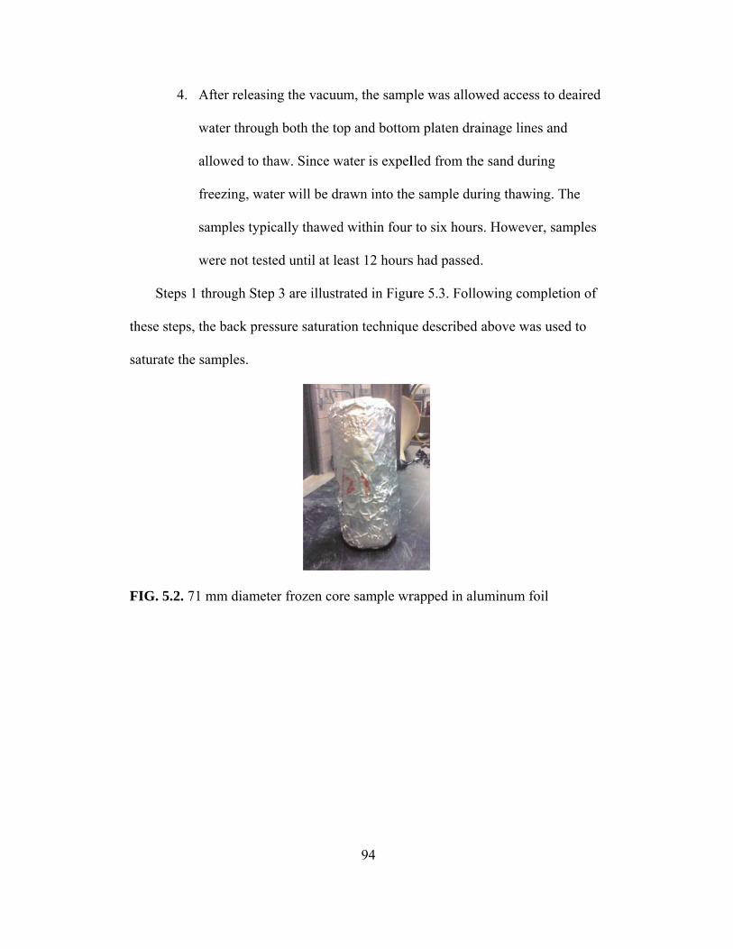
th
sa
F
4. A
w
al
fr
sa
w
Steps 1 th
hese steps, th
aturate the sa
FIG. 5.2. 71 m
After releasin
water through
llowed to tha
reezing, wate
amples typic
were not teste
hrough Step
he back pres
amples.
mm diamete
ng the vacuu
h both the to
aw. Since w
er will be dr
cally thawed
ed until at le
3 are illustr
sure saturati
er frozen cor
94
um, the samp
op and bottom
water is expel
rawn into the
d within four
east 12 hours
rated in Figu
ion techniqu
re sample wr
ple was allow
m platen dra
lled from the
e sample dur
r to six hours
s had passed
ure 5.3. Follo
ue described
rapped in alu
wed access to
ainage lines a
e sand during
ring thawing
s. However,
d.
owing compl
above was u
uminum foil
o deaired
and
g
g. The
samples
letion of
used to

F
tr
m
ch
5
d
an
te
o
co
bu
st
d
FIG. 5.3. 71 m
rimming; (b)
membrane wi
hamber in pl
.2.3 Triaxi
The GCT
evice. Follow
n internal GC
est (drained o
f the test, an
ollected ever
ut tests were
tress was ob
ecrease.
(a)
mm diamete
) Frozen sam
ith vacuum c
lace.
ial Tests and
TS system is
wing back p
CTS system
or undrained
nd strain rate
ry second du
e regularly te
served to ha
er sample pre
mple mounted
confining pr
d Data Acqu
equipped w
ressure satur
m program tha
d), type of lo
. The strain
uring the test
erminated a
ave occurred
95
(b)
eparation for
d on triaxial
essure appli
isition
with a compu
ration, triaxi
at specifies,
oading, data
rate was pre
t. The end o
few percent
, i.e. after th
r testing: (a)
l cell and con
ed; (c) Froze
uter and digit
ial testing w
among othe
acquisition r
esented in Se
f test was sp
strain after t
he deviator st
(c)
) Frozen sam
nfined in late
en sample w
tal signal co
was conducted
er things, the
rate, strain a
ection 5.1. D
pecified as 1
the peak dev
tress began t
mple after
ex
with cell
ntrol
d using
e type of
at the end
Data was
5% strain
viator
to
96
5.2.4 Problems Encountered During Testing
Initially, 35 mm diameter frozen core samples were recovered from the
model box. However, the results of the triaxial compression tests on the 35 mm-
diameter specimens were inconsistent with the tests performed on 71 mm
diameter, never frozen specimens. Furthermore, results of the tests on the 35 mm
diameter specimens were very hard to reproduce. There was wide variability in
the results from the 35 mm-diameter specimens. This variability was attributed to
the size of the sample. In order to reduce the variability, it was decided to recover
71 mm diameter samples from the model box for all triaxial testing.
Soil microstructure studies performed on the 35 mm samples obtained using
the methods described in this work did not show variability in microstructure
commensurate with the variability that was observed in the triaxial tests (Czupak,
2011). Therefore, for purposes of the microstructure studies, recovery of 35 mm-
diameter samples continued throughout the course of this work.
5.3 Drained Tests Results
5.3.1 Never Frozen Sand Tests Results
The results of five consolidated drained triaxial tests conducted on never
frozen specimens of Ottawa 20-30 sand prepared by air pluviation are presented
in this section. The initial densities of the tests are presented in Table 5-2. The
drained stress-strain-strength characteristics of these never frozen Ottawa 20-30
sand specimens are presented in Figure 5.4. The volume change-strain behavior
during these tests is presented in Figure 5.5.
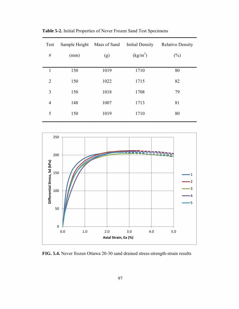
97
Table 5-2. Initial Properties of Never Frozen Sand Test Specimens
Test
#
Sample Height
(mm)
Mass of Sand
(g)
Initial Density
(kg/m3)
Relative Density
(%)
1 150 1019 1710 80
2 150 1022 1715 82
3 150 1018 1708 79
4 148 1007 1713 81
5 150 1019 1710 80
FIG. 5.4. Never frozen Ottawa 20-30 sand drained stress-strength-strain results
0
50
100
150
200
250
0.0 1.0 2.0 3.0 4.0 5.0
Differential Stress, Sd (kPa)
Axial Strain, Ea (%)
1
2
3
4
5

98
FIG. 5.5. Never frozen sand volume strain-axial strain results
5.3.2 Frozen and Thawed Test Results
Four recovered cores were tested to develop stress-strain-strength behavior of
frozen and thawed sand. The initial densities of the recovered samples that were
determined by weighing oven dried sand after testing are shown in Table 5-3. The
stress-strain-strength behavior in drained triaxial compression tests conducted on
four recovered frozen cores of Ottawa 20-30 sand after thawing is presented in
Figure 5.6. The volume change-strain behavior during these tests is presented in
Figure 5.7.
‐4.50
‐4.00
‐3.50
‐3.00
‐2.50
‐2.00
‐1.50
‐1.00
‐0.50
0.00
0.50
0.0 1.0 2.0 3.0 4.0 5.0 6.0Volumetric Strain, Ev (%
)
Axial Strain, Ea (%)
1
2
3
4
5

99
Table 5-3. Initial Properties of Frozen Core Test Specimens
Test
# Sample Height (mm)
Mass of Sand
(g)
Initial Density
(kg/m3)
Relative
Density
(%)
1 144 977 1705 78
2 145 983 1707 79
3 144 977 1708 79
4 148 1005 1710 80
FIG. 5.6. Results of drained triaxial compression tests on recovered frozen cores
of Ottawa 20-30 sand samples
0
50
100
150
200
250
0.0 0.5 1.0 1.5 2.0 2.5 3.0 3.5 4.0 4.5 5.0
Deviator Stress, Sd (kPa)
Axial Strain, Ea (%)
1
2
3
4

100
FIG. 5.7. Drained volume change-Strain results
5.3.3 Comparison of the Drained Triaxial Compression Test Results
The results of the triaxial compression tests conducted on never frozen sand
and on the recovered frozen samples after thawing were compared, to determine
whether the frozen and then thawed sand retains its drained deformation
characteristics. The results of this comparison serve as an indication of the level
of disturbance due to the sampling techniques developed in this work.
Mean stress-strain-strength and volume curves were developed from the two
groups of curves (never frozen, and frozen and then thawed) from the drained
triaxial testing. The two median stress-strain-strength curves are shown in Figure
‐4
‐3.5
‐3
‐2.5
‐2
‐1.5
‐1
‐0.5
0
0.5
0 1 2 3 4 5
Volumetric Strain, Ev (%
)
Axial Strain, Ea (%)
1
2
3
4
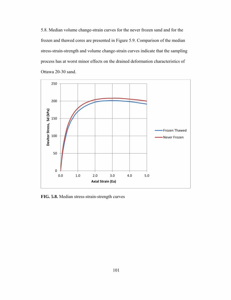
101
5.8. Median volume change-strain curves for the never frozen sand and for the
frozen and thawed cores are presented in Figure 5.9. Comparison of the median
stress-strain-strength and volume change-strain curves indicate that the sampling
process has at worst minor effects on the drained deformation characteristics of
Ottawa 20-30 sand.
FIG. 5.8. Median stress-strain-strength curves
0
50
100
150
200
250
0.0 1.0 2.0 3.0 4.0 5.0
Devitor Stress, Sd
(kPa)
Axial Strain (Ea)
Frozen Thawed
Never Frozen
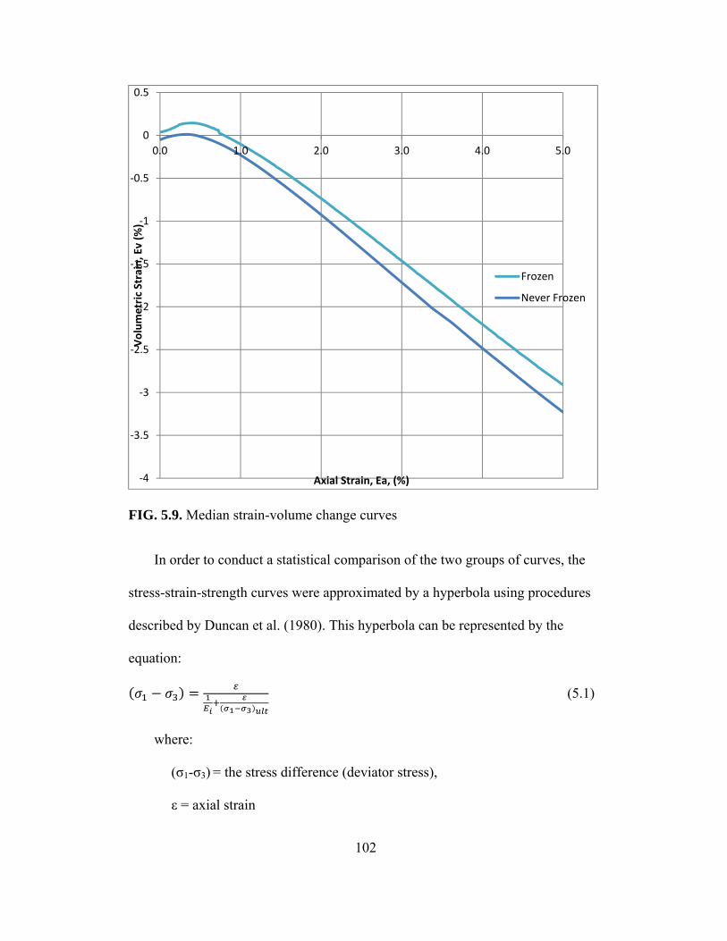
102
FIG. 5.9. Median strain-volume change curves
In order to conduct a statistical comparison of the two groups of curves, the
stress-strain-strength curves were approximated by a hyperbola using procedures
described by Duncan et al. (1980). This hyperbola can be represented by the
equation:
(5.1)
where:
(σ1-σ3) = the stress difference (deviator stress),
ε = axial strain
‐4
‐3.5
‐3
‐2.5
‐2
‐1.5
‐1
‐0.5
0
0.5
0.0 1.0 2.0 3.0 4.0 5.0Volumetric Strain, Ev (%
)
Axial Strain, Ea, (%)
Frozen
Never Frozen

103
Ei = the initial tangent modulus, and
(σ1-σ3)ult = the asymptotic value of stress difference for the fitted
hyperbola.
The value of (σ1-σ3)ult is usually greater than the strength mobilized in a triaxial
test, (σ1-σ3)f. Therefore, Duncan et al. (1980) defined a third parameter Rf to
analytically describe a stress-strain curve, where Rf was defined as the ratio of the
mobilized strength to (σ1-σ3)ult:
Rf = (σ1-σ3)f /(σ1-σ3)ult (5.2)
As described by Duncan et al. (1980), two points (typically, points corresponding
to 70% and 95% of the strength mobilized in the test) from each stress-strain
curve were used to derive the two variables (Ei and (σ1-σ3)ult ) that describe the
hyperbola.
In order to compare the volume change curves, three parameters were
abitrarily chosen for comparison. The volume change at 70 %, 95 % and at 100%
of the strength mobilized in the test were the chosen parameters. Therefore, in
total, six parameters derived from the drained triaxial compression tests were
employed to compare test results: three parameters describing the volume change-
strain characteristics and three parameters decribing the stress-strain-strength
characteristics.
A statistical comparison of the six parameters was conducted for the two
groups of drained triaxial test results. The statistical analyses used a t-distribution
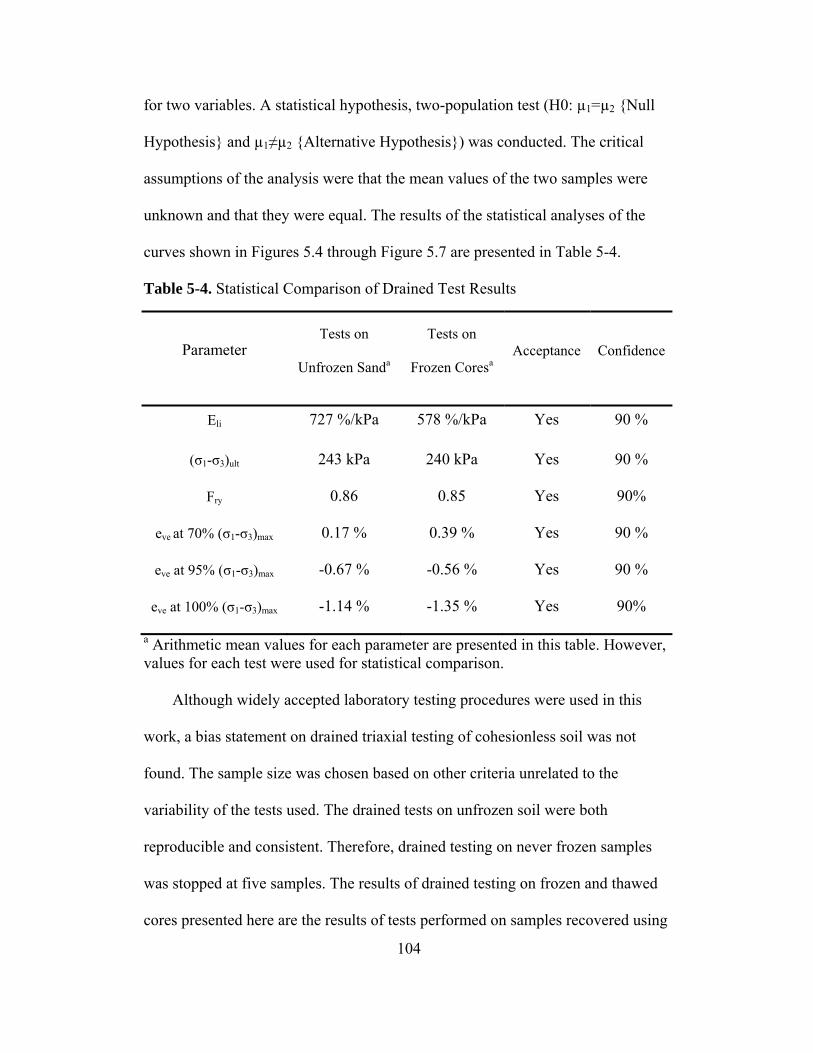
104
for two variables. A statistical hypothesis, two-population test (H0: µ1=µ2 {Null
Hypothesis} and µ1≠µ2 {Alternative Hypothesis}) was conducted. The critical
assumptions of the analysis were that the mean values of the two samples were
unknown and that they were equal. The results of the statistical analyses of the
curves shown in Figures 5.4 through Figure 5.7 are presented in Table 5-4.
Table 5-4. Statistical Comparison of Drained Test Results
Parameter Tests on
Unfrozen Sanda
Tests on
Frozen Coresa Acceptance Confidence
Eli 727 %/kPa 578 %/kPa Yes 90 %
(σ1-σ3)ult 243 kPa 240 kPa Yes 90 %
Fry 0.86 0.85 Yes 90%
eve at 70% (σ1-σ3)max 0.17 % 0.39 % Yes 90 %
eve at 95% (σ1-σ3)max -0.67 % -0.56 % Yes 90 %
eve at 100% (σ1-σ3)max -1.14 % -1.35 % Yes 90%
a Arithmetic mean values for each parameter are presented in this table. However, values for each test were used for statistical comparison.
Although widely accepted laboratory testing procedures were used in this
work, a bias statement on drained triaxial testing of cohesionless soil was not
found. The sample size was chosen based on other criteria unrelated to the
variability of the tests used. The drained tests on unfrozen soil were both
reproducible and consistent. Therefore, drained testing on never frozen samples
was stopped at five samples. The results of drained testing on frozen and thawed
cores presented here are the results of tests performed on samples recovered using

105
the Husqvarna DR 150 core drill rig. The statistical comparison of this limited
sample size shows that the two groups of tests are the same at a confidence of
90%. It can be concluded from the results that the sampling process produces
undisturbed samples that retain their drained deformation characteristics.
5.4 Undrained Test Results
5.4.1 Never Frozen Sand Test Results
The results of five consolidated undrained triaxial tests conducted on never
frozen specimens of Ottawa 20-30 sand prepared by air pluviation to a relative
density of approximately 80% are presented in this section. The initial densities of
the tests are presented in Table 5-5. The undrained stress-strain-strength behavior
of never frozen Ottawa 20-30 sand specimens tested in triaxial compression are
presented in Figure 5.10. The excess pore pressure-strain results during the
undrained triaxial tests are presented in Figure 5.11.
Table 5-5. Initial Properties of Undrained Baseline Tests Specimens
Test
# Sample Height (mm)
Mass of Sand
(g)
Initial Density
(kg/m3)
Relative Density
(%)
1 150 1019 1710 80
2 149 1013 1712 81
3 150 1012 1714 82
4 150 1019 1710 80
5 149 1012 1710 80

106
FIG. 5.10 Never frozen Ottawa 20-30 sand undrained stress-strength-strength
results
0
100
200
300
400
500
600
700
800
900
0 2 4 6 8
Deviator Stress, Sd (kPa)
Axial Strain, Ea (%)
1
2
3
4
5
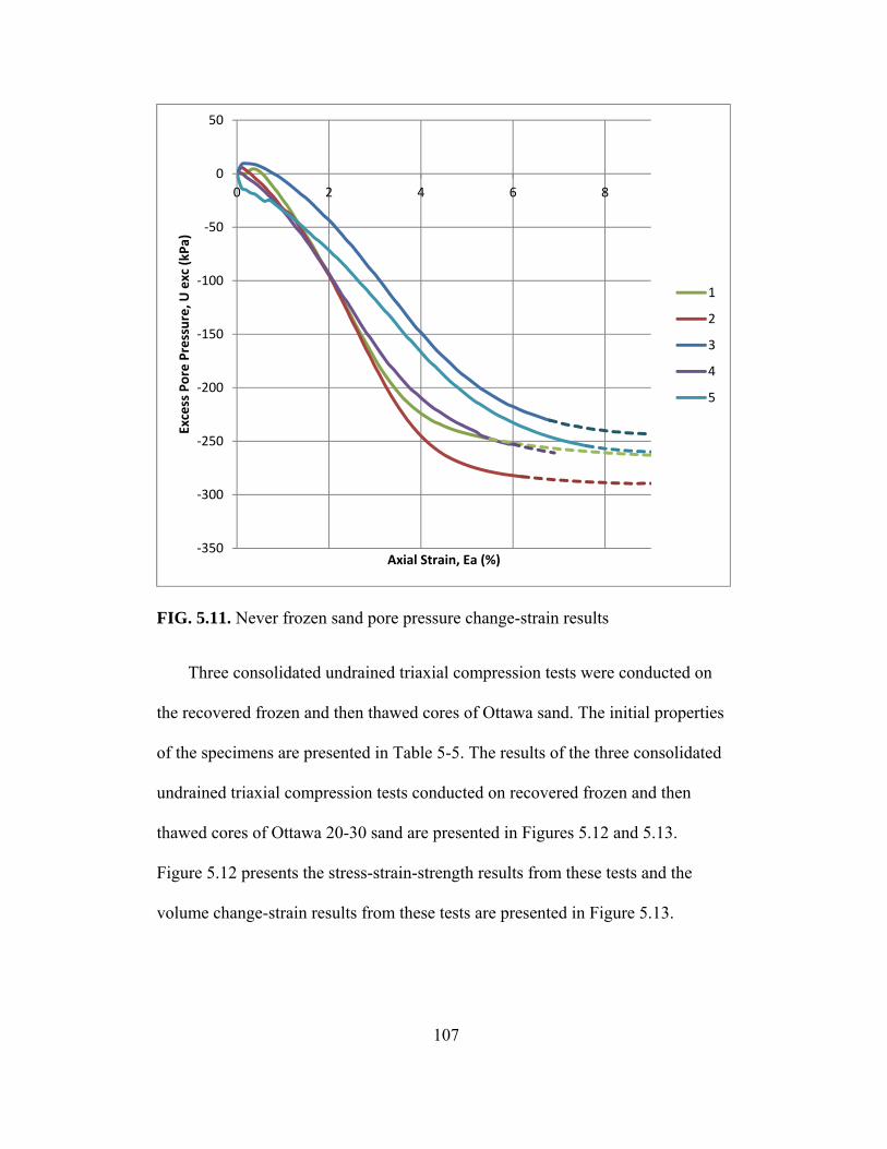
107
FIG. 5.11. Never frozen sand pore pressure change-strain results
Three consolidated undrained triaxial compression tests were conducted on
the recovered frozen and then thawed cores of Ottawa sand. The initial properties
of the specimens are presented in Table 5-5. The results of the three consolidated
undrained triaxial compression tests conducted on recovered frozen and then
thawed cores of Ottawa 20-30 sand are presented in Figures 5.12 and 5.13.
Figure 5.12 presents the stress-strain-strength results from these tests and the
volume change-strain results from these tests are presented in Figure 5.13.
‐350
‐300
‐250
‐200
‐150
‐100
‐50
0
50
0 2 4 6 8Excess Pore Pressure, U
exc (kPa)
Axial Strain, Ea (%)
1
2
3
4
5
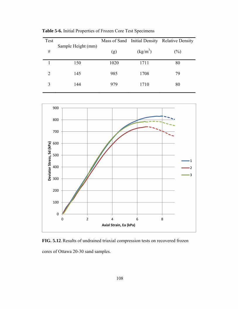
108
Table 5-6. Initial Properties of Frozen Core Test Specimens
Test
# Sample Height (mm)
Mass of Sand
(g)
Initial Density
(kg/m3)
Relative Density
(%)
1 150 1020 1711 80
2 145 985 1708 79
3 144 979 1710 80
FIG. 5.12. Results of undrained triaxial compression tests on recovered frozen
cores of Ottawa 20-30 sand samples.
0
100
200
300
400
500
600
700
800
900
0 2 4 6 8
Deviator Stress, Sd (kPa)
Axial Strain, Ea (kPa)
1
2
3

109
FIG. 5.13. Pore pressure change-axial strain results
5.4.2 Comparison of the Undrained Triaxial Compression Test Results
The results of the undrained triaxial compression tests conducted on never
frozen sand and on the recovered frozen and then thawed samples were compared
to determine whether the sampled sand retains its undrained deformation
characteristics.
The Duncan et al. (1980) stress-strain curve fitting equation was not used for
statistical comparison of undrained triaxial test results. The curve fitting equation
was developed from drained tests. An attempt to use this curve fitting method on
undrained tests was made. The curve fitting method produced unrealistic numbers
‐300
‐250
‐200
‐150
‐100
‐50
0
50
0 2 4 6 8Deviator Stress, Sd (kPa)
Axial Strain, Ea (%)
1
2
3

110
e.g. Rf of 0.37, when the typical range for sands is 0.5 to 0.9. For this reason, it
was decided not to use the Duncan et al. curve fitting method on undrained tests
results.
An alternative comparison method was used for undrained test results. The
mean undrained stress-strain-strength curve was developed from the baseline
undrained triaxial compression tests performed on never frozen sand. Standard
deviations of the deviator stress at discrete strain levels were calculated from the
five baseline tests. A confidence interval was developed that was bound at the top
by the mean plus two standard deviations and at the bottom by the mean minus
two standard deviations. The frozen/thawed tests results were plotted on the
confidence interval plot to demonstrate how well the results on the recovered
samples compared with the baseline results. The stress-strain-strength comparison
figure is presented in Figure 5.14. The excess pore pressure-strain results were
compared using methods used to compare stress-strain-strength behavior
(described previously). The results of the comparison are presented in Figure
5.15.
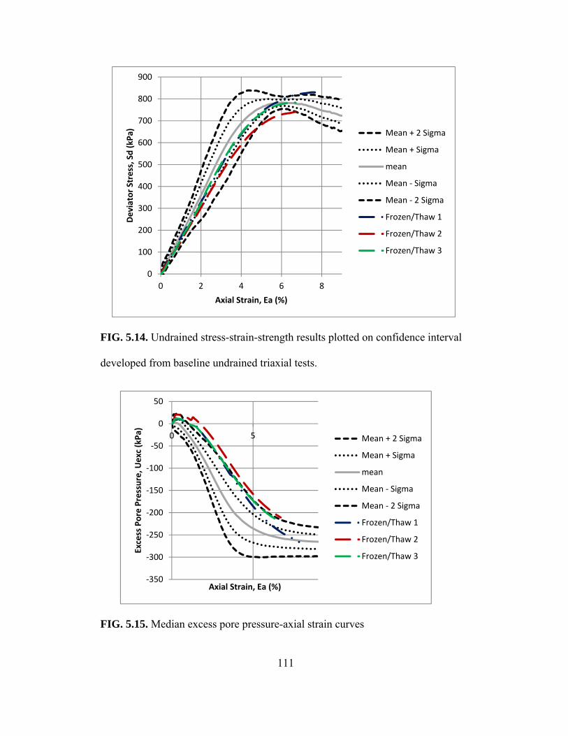
111
FIG. 5.14. Undrained stress-strain-strength results plotted on confidence interval
developed from baseline undrained triaxial tests.
FIG. 5.15. Median excess pore pressure-axial strain curves
0
100
200
300
400
500
600
700
800
900
0 2 4 6 8
Deviator Stress, Sd (kPa)
Axial Strain, Ea (%)
Mean + 2 Sigma
Mean + Sigma
mean
Mean ‐ Sigma
Mean ‐ 2 Sigma
Frozen/Thaw 1
Frozen/Thaw 2
Frozen/Thaw 3
‐350
‐300
‐250
‐200
‐150
‐100
‐50
0
50
0 5
Excess Pore Pressure, U
exc (kPa)
Axial Strain, Ea (%)
Mean + 2 Sigma
Mean + Sigma
mean
Mean ‐ Sigma
Mean ‐ 2 Sigma
Frozen/Thaw 1
Frozen/Thaw 2
Frozen/Thaw 3

112
The results of the undrained tests conducted on never frozen sand and on
recovered cores were also analyzed by comparing the stress and excess pore water
pressure at three strain levels: at one percent, three percent, and five percent
strain. The three strain levels were chosen arbitrarily. The three strain levels were
assumed to represent the stress-strain-strength, and the excess pore pressure-strain
relationship developed from the consolidated undrained test results data.
A statistical comparison of the parameters was conducted for the two groups
of undrained triaxial test results. The statistical analyses used a t-distribution for
two variables. A statistical hypothesis, two-population test (H0: µ1=µ2 {Null
Hypothesis} and µ1≠µ2 {Alternative Hypothesis}) was conducted. The critical
assumptions of the analysis were that the mean values of the two samples were
unknown and that they were equal. The results of the statistical analyses of the
curves shown in Figures 5.10 through Figure 5.13 are presented in Table 5.7 and
Table 5-8.
Table 5-7. Statistical Comparison of Deviator Stress – Strain Results
Parameter Tests on
Unfrozen Sanda Tests on frozen Sanda
Acceptance at 90%
confidence
Sd at 1% 171 kPa 158 kPa Yes
Sd at 3% 526 kPa 486 kPa Yes
Sd at 5% 749 kPa 719 kPa Yes
a Arithmetic mean values for each parameter are presented in this table. However, values for each test were used for statistical comparison.

113
Table 5-8. Statistical Comparison of Excess Pore Water Pressure - Strain Results
Parameter Tests on
Unfrozen Sanda
Tests on frozen
Sanda
Acceptance at
90% confidence
Acceptance at
95% confidence
Uexc at 1% -26 kPa 3 kPa No No
Uexc at 3% -145 kPa -77 kPa No Yes
Uexc at 5% -230 kPa -173 kPa Yes Yes
a Arithmetic mean values for each parameter are presented in this table. However, values for each test were used for statistical comparison. The undrained tests on both never frozen sand and on recovered cores
showed a lot of variability and were very difficult to reproduce. The stress-strain-
strength behavior and excess pore water pressure developed during undrained
triaxial loading is dependent on the level of saturation, the pore fluid stiffness, and
the void ratio at the beginning of the tests. According to William Houston,
undrained shear strength of saturated or nearly saturated sand is generally elusive
and hard to reproduce (Personal communication, June 3, 2011). This variability
and difficulty to reproduce the shear strength is attributable to the difficulty to
produce specimens of sand that have identical B-values, identical degrees of
saturation and, identical pore fluid stiffness in the laboratory (W. Houston,
Personal communication, June 3, 2011).
The results of the tests conducted on recovered cores compare favorably
with the baseline deformation behavior in undrained triaxial loading that was
established from the five undrained tests conducted on never frozen Ottawa 20-30
sand. The differences observed between the two sets of tests (tests of unfrozen
sand and tests on recovered cores) are well within the variability in the test results
114
observed during testing and also within the results, that can be expected from
undrained triaxial testing of saturated sand. It can be concluded from the results
that the sampling process has at most only minimal effects on the undrained
deformation characteristics of saturated Ottawa sand. The sampling procedure
described in this work produces undisturbed samples that retain their undrained
deformational characteristics.

115
Chapter 6
6.0 CONCLUSIONS AND RECOMMENDATIONS
6.1 Conclusions
The main objective of this work was to develop a method for recovering
undisturbed samples of cohesionless soil from physical models. This work is part
of a larger project to experimentally and numerically investigate the properties of
resedimented cohesionless soil following earthquake induced liquefaction. The
work presented in this thesis resulted in the development of a practical method for
preparing uniform soil deposits in laboratory bench scale and centrifuge models
and the development of a practical method of recovering intact and essentially
undisturbed samples of cohesionless soil from these physical models.
The technique for preparation of uniform sand specimens was developed
based on methods used by Frost (1989) and also by UC Davis. The technique is
based on air pluviation. A pluviation apparatus was developed that allows for
creation of samples of Ottawa 20-30 sand samples at target densities by varying
the height of fall of the sand. The apparatus is simple, can be created from easily
obtainable parts, and does not require specialized fabrication. A calibration curve
for the pluviation apparatus was developed relating fall height to the post-
placement density of Ottawa 20-30 sand. Using this technique, specimens of
Ottawa 20-30 sand can be created in containers of varying sizes at densities
ranging from 1,550 kg/m3 to 1,730 kg/m3 (96 lb/ft3 to 108 lb/ft3).
116
A method for recovering undisturbed samples of cohesionless soil from
laboratory bench scale models was developed. The technique can also be used on
centrifuge- and shaking table-scale models. The sampling method involved
stabilization of cohesionless soil by freezing and recovery of samples by coring.
A freezing method was developed that used crushed dry ice and ethanol placed in
a metal pan as a coolant. The temperature of the mixture of dry ice and ethanol
was measured to be -68°C. The pan filled with coolant was placed on top of the
saturated model specimen, from which samples were to be recovered, inducing a
top-down freezing front.
The propagation of the freezing front that was induced by the chosen freezing
method was experimentally and numerically investigated. A unidirectional
freezing front, a surcharge, and a drainage path in the direction of the freezing
front are requirements for the freezing of cohesionless soil with minimal volume
change. The results of the experimental and numerical investigations showed that
these requirements were met by the technique employed herein. The freezing
front propagated from top to bottom without the development of any secondary
freezing fronts with the potential to trap water between impermeable (or very low
permeability) surfaces. The drainage path was maintained through the bottom of
the model container and through the sides between the walls of the container and
the frozen portion of the specimen during the freezing process. Water was
observed flowing from the container over the sides as the specimen froze. The
weight of the pan and coolant appeared to provide adequate surcharge pressure on
the specimen to limit expansion during freezing. Significant expansion of the

117
cohesionless soil models was not observed during numerous freezing experiments
conducted in this work.
Equipment for coring 35 mm diameter and 71 mm diameter samples of
frozen cohesionless soil was developed. Using this equipment, numerous samples
were successfully recovered from the physical models. The sampling methods are
simple and can be replicated at different locations without requiring sophisticated
fabrication effort.
The undisturbed nature of the samples was investigated using triaxial
compression tests. Drained and undrained triaxial compression tests were
performed on never frozen Ottawa 20-30 sand pluviated to create a specimen with
a relative density of 80% to establish baseline deformation characteristics.
Recovered frozen cores were confined in a triaxial cell and allowed to thaw. The
same tests that were performed on never frozen Ottawa 20-30 sand specimens
were then performed on the thawed cores. The results of the tests on never frozen
and frozen and then thawed specimens were compared to assess the undisturbed
nature of the samples obtained using the sampling techniques developed in this
work.
Based on the experiment results and analyses reported in this thesis, it can be
concluded that the samples recovered using the sampling techniques developed in
this work retain their original drained and undrained deformation characteristics.
The freezing and thawing process has only minimal effects on the deformation
characteristics of the Ottawa 20-30 cohesionless soil. The differences between
deformational characteristic of never frozen sand and frozen and thawed sand

118
appear to be within the normal variation that can be expected from testing
different samples of the same soil.
6.2 Recommendations
The specimen creation and sampling techniques presented in this work are
suitable for use in the larger project and projects of similar scope and size. Based
on the testing conducted in this work, the samples obtained using methods
described in this thesis can reasonably be expected to maintain their structure and
deformational characteristics. However, there are a number of other factors that
were not addressed in this work that might have bearing on the quality of samples
obtained using methods described herein.
The effect of the moisture content of the dry sand on the pluviation technique
was not addressed in this work. Although, samples with consistent density were
produced using the pluviation method, the moisture content of the sand was not
considered during sample creation. Future testing could be performed using oven
dried sand in order to maintain constant moisture content during sample
preparation.
The ASTM standard for consolidated drained triaxial compression tests (CD
tests) does not have a bias or variability statement. Data on the bias and variability
of the CD test was not found in the literature. The number of tests performed on
never frozen sand in this study was relatively small. Although the test results were
fairly consistent and easily reproducible, the number of tests was too small to
confidently establish bias and variability of the CD test. Future studies could
119
perform more tests to develop a better estimate of the bias and variability of the
test.
A test standard for the consolidated undrained triaxial compression tests (CU
test) was not found in the literature. The results of the testing conducted in this
research showed that the CU test results showed greater variability than the CD
test results. It seems the CU test is more sensitive to small variability in initial
specimen density and saturation level (B-value). This variability made the CU test
a difficult method to use for purposes of investigating the deformation
characteristics of sampled cohesionless soil. The number of samples tested in this
study is relatively small. Future study could focus on conducting a statistically
significant number of CU tests in order to develop an estimate of the bias and
variability for the test itself. The CU test bias and variability, could lead to better
comparisons of deformation characteristics of never frozen sand and frozen sand.
The CU test bias and variability could also be applied in other cases where CU
test on cohesionless soil may be required.
This research was interested in investigating the large strain behavior,
consistent with the focus of the larger project (post liquefaction properties of
cohesionless soil). Future research could investigate the effects of freezing and
thawing on small strain behavior e.g. by measuring shear wave velocity in never
frozen specimens and also in frozen and then thawed specimens.
Poorly graded Ottawa 20-30 sand was used in this work. The sand has
uniform sub-rounded particles. Future research could perform the tests conducted
in this work using graded sand with sub-rounded particles, and also using sand

120
with angular particles. This research could investigate the effect of changing the
test soil on expansion due to freezing, deformation characteristics of frozen and
thawed soil, and creation of uniform deposits of sand using the pluviation
techniques described in this work.
Another area of additional study is the effect of the sampling techniques on
the ‘aging effect’ of sands described by Mitchell (2008). Future research could
investigate whether cohesionless soil sampled using freezing loses strength gained
through aging. This research could provide insight to whether samples obtained
from an aged deposit of sand would retain its aged strength gain, i.e. whether
freezing followed by thawing erases aging effects.

121
7.0 REFERENCES
Alshibli, K. A., Sture, S., Costes, N. C., Frank, M. L., Lankton, M. R., Batiste, S. N., et al. (2000, September). Assessment of Localized Deformations in Sand Using X-Ray Computed Tomography. Geotechnical Testing Journal, 23(3), 274-299.
Araki, C. (1956). Structure of agarose, a main polysaccharide of agar-agar. memoirs of the faculty of industrial arts, 21-25.
Borja, R. I., Kavazanjian, E., & Evans, J. C. (2008). Properties of Cohesionless Soil Subsequent Liquefaction and Resedimentation. Proposal.
Czupak, Z. D. (2011). "Stabilization and Imaging of Cohesionless Soil Samples". Tempe: Arizona State University.
Czupak, Z. D. (2011). Stabilization and Imaging of Cohesionless Soil Samples. Tempe: Arizona State University.
Duncan, J. M., Byrne, P., Wong, K. S., & Mabry, P. (1980). Strength, Stress-Strain and Bulk Modulus Parameters for Finite Element Analyses of Stresses and Movements in Soil Masses. Berkeley: University of California at Berkeley.
Evans, M. T. (2005). Microscale Physical and Numerical Investigations of Shear Banding in Granular Soils. Atlanta: Georigia Institute of Technology.
Fiegel, G. L., Hudson, M., Idriss, I. M., Kutter, L. B., & Zeng, X. (1994). Effect of model containers on dynamic soil response. In Leung, Lee, & Tan (Ed.), Centrifuge 94 (pp. 145-150). Rotterdam: Balkema.
Frost, J. D. (1989). Studies on the Monotonic and Cyclic Behavior of Sands. West Lafayette: Purdue University.
GCTS Testing Systems. (2005). CATS Advanced and Universal 1.89. Tempe: GCTS Testing Systems.
Holtz, R. D., & Kovacs, W. D. (1981). "An Introduction to Geotechnical Engineering". Englewood Cliffs: Prentice Hass.
Holtz, R. D., & Kovacs, W. D. (1981). An Introduction to Geotechnical Engineering. Englewood Cliffs: Prentice Hass.
Hvorslev, J. M. (1949). Subsurface Exploration and Sampling of Soils for Civil Engineering Purposes. Vicksburg: Waterways Experiment Station.
122
Mitchell, J. K. (2008). Aging of Sand - A Continuing Enigma? 6th International Conference on Case Histories in Geotechnical Engineering (pp. 1-21). Arlington: Virginia Tech.
Mitchell, J. K., & Soga, K. (2005). Fundamentals of Soil Behavior (3rd ed.). Hoboken, New Jersey: John Wiley & Sons, Inc.
Miura, S., & Toki, S. (1982). A Sample Preparation Method and its Effect on Static and Cyclic Deformation Strength Properties of Sand. Soils and Foundation, 61-77.
Mulilis, P. J., Chan, C. K., & Seed, B. H. (1975). The Effects of Method of Sample Preparation on the Cyclic Stress-Strain Behavior of Sands. Berkeley: University of California, Barkeley.
Salgado, R., Bandini, P., & Karim, A. (2000). Shear Strength and Stiffness of Silty Sand. Journal of Geotechincal and Geoenvironmental Engineering, 451-462.
Santamarina, C. J., & Cho, C. G. (2001, June). Determination of Critical State Parameters in Sandy Soils - Simple Procedure. Geotechnical Testing Journal, 24(2), 185-192.
Schneider, H. R., Chameau, J.-L., & Leonards, G. A. (1989). Chemical Impreganation of Cohesionless Soils. Geotechnical Testing Journal, 12(3), 204-210.
Singh, S., Seed, B. H., & Chan, C. K. (1982). Undisturbed Sampling of Saturated Sands by Freezing. Journal of Geotechnical Engineering, 247-264.
Soil Vision. (2010). SVHeat User's Manual. Saskatoon: Soil Vision Systems Limited.
Sutterer, K. G., Frost, D. J., & Chameau, J.-L. A. (1995). Polymer Impregnation to Assist Undistrurbed Sampling of Cohesionless Soils. Journal of Geotechnical Engineering, 209-215.
Tystovich, N. (1952). Principles of the Mechanics of Frozen Soils. Academy of Sciences, U.S.S.R.
Ueno, K. (2000). "Methods for Preparation of Sand Samples". In Kusakabe, & Takemura (Ed.), Centrifuge 98 (pp. 1047-1055). Tokyo: Balkema.
Yang, C.-T. (2002). Boundary Condition and Inherent Stratigraphic Effects on Microsctructure Evolution in Sand Specimen. Georgia Institute of Technology. Atlanta: Georigia Institute of Technology.

123
Yoshimi, Y., Hatanaka, M., & Oh-Oka, H. (1978). Undisturbed Sampling of Saturated Sands by Freezing. Soils and Foundation, 59-73.

124
APPENDIX A
DESIGN DRAWINGS FOR THE BOX USED IN FREEZING AND
SAMPLING EXPERIMENTS, AND OTHER FABRICATED EQUIPMENT

125
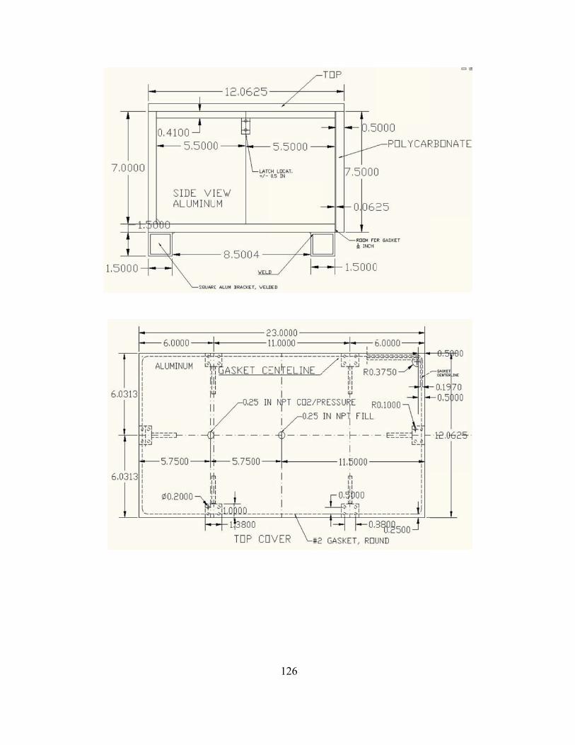
126

127

1
A
P
. DRILL G
Assembly
art 1 – Made
GUIDE – All
e out of Alum
Dimensions
minum
128
s are in inches.
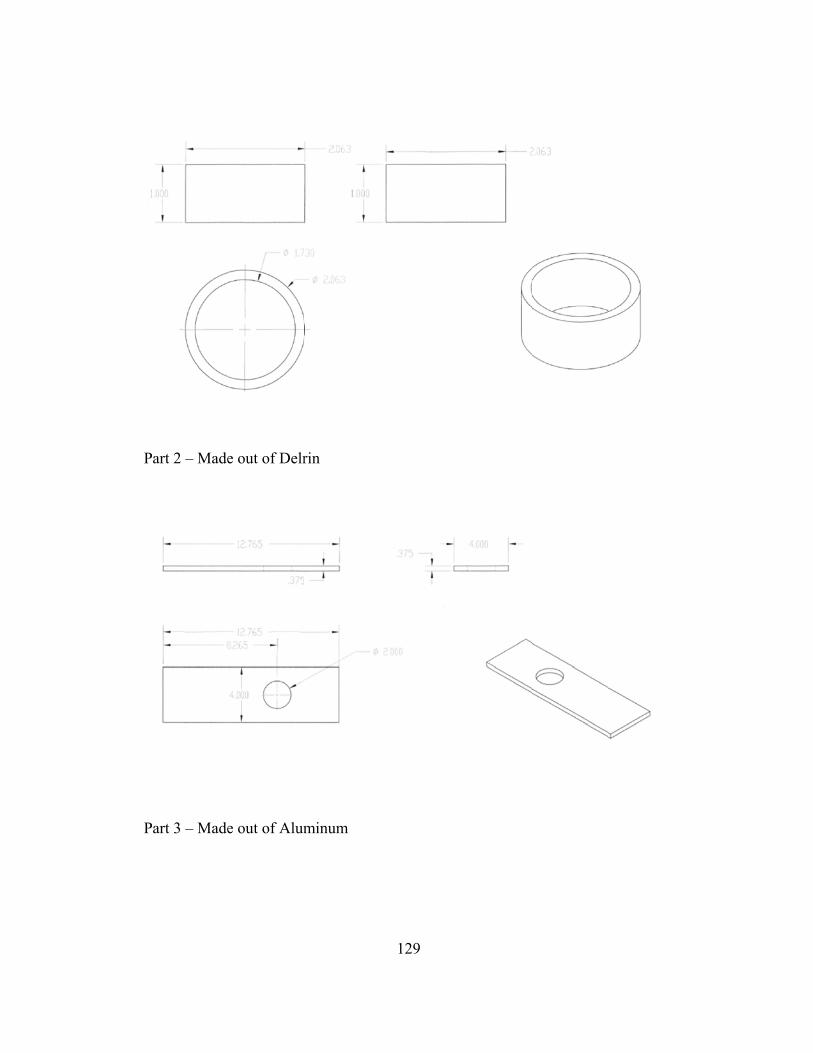
P
P
art 2 – Made
art 3 – Made
e out of Delr
e out of Alum
rin
minum
129
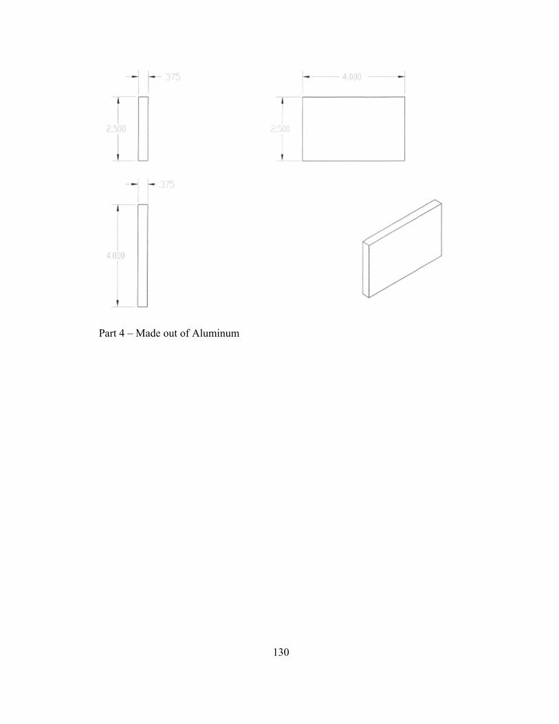
P
art 4 – Madee out of Alumminum
130

131
APPENDIX B
TRIAXIAL TESTS RESULTS AND EVALUATIONS

Initial Properties of Never Frozen Sand Test Specimens
Test
#
Sample
Height
(mm)
Mass of
Sand
(g)
Initial
Density
(kg/m3)
Relative
Density
(%)
B-Value
1 150 1019 1710 80 0.95
2 150 1022 1715 82 0.97
3 150 1018 1708 79 0.95
4 148 1007 1713 81 0.96
5 150 1019 1710 80 0.94
132

Never frozen San
d Tests Data
EaS d
EvEa
S dEv
EaS d
EvEa
S dEv
EaS d
EvEa
SdEv
0.0
0‐0.05
0.0
00.0
0.0
0‐0.1
0.0
0‐0.1
0.0
0‐0.1
0.0
0‐0.1
0.2
103
‐0.02
0.2
73
0.1
0.2
68
‐0.1
0.0
23
0.0
0.2
71
0.0
0.1
67
0.0
0.4
151
‐0.03
0.4
127
0.1
0.4
123
‐0.1
0.2
75
0.1
0.4
120
0.0
0.4
119
0.0
0.6
171
‐0.11
0.6
158
0.1
0.6
149
‐0.1
0.5
112
0.1
0.6
149
‐0.1
0.6
148
0.0
0.8
184
‐0.21
0.8
173
0.0
0.8
165
‐0.2
0.7
141
0.0
0.8
167
‐0.1
0.8
166
‐0.1
1.0
192
‐0.34
1.0
184
‐0.2
1.0
176
‐0.3
0.9
162
0.0
1.0
179
‐0.2
1.0
179
‐0.2
1.2
197
‐0.48
1.2
192
‐0.3
1.2
183
‐0.4
1.1
176
‐0.2
1.2
187
‐0.4
1.2
187
‐0.3
1.4
201
‐0.62
1.4
198
‐0.4
1.4
189
‐0.6
1.3
186
‐0.3
1.4
194
‐0.5
1.4
194
‐0.5
1.6
203
‐0.77
1.6
202
‐0.6
1.6
193
‐0.7
1.5
193
‐0.4
1.6
199
‐0.7
1.6
198
‐0.6
1.8
206
‐0.93
1.8
205
‐0.8
1.8
197
‐0.9
1.7
198
‐0.6
1.8
202
‐0.8
1.8
202
‐0.8
2.1
207
‐1.09
2.1
208
‐0.9
2.1
200
‐1.0
1.9
202
‐0.7
2.1
205
‐1.0
2.0
204
‐0.9
2.3
207
‐1.24
2.3
209
‐1.1
2.3
201
‐1.2
2.1
205
‐0.9
2.3
206
‐1.1
2.2
206
‐1.1
2.5
208
‐1.40
2.5
211
‐1.3
2.5
203
‐1.4
2.3
207
‐1.0
2.5
207
‐1.3
2.4
207
‐1.3
2.7
208
‐1.55
2.7
212
‐1.4
2.7
204
‐1.5
2.5
208
‐1.2
2.7
208
‐1.4
2.6
208
‐1.4
2.8
207
‐1.68
2.8
212
‐1.5
2.8
204
‐1.6
2.7
209
‐1.3
2.8
209
‐1.6
2.8
208
‐1.6
3.0
206
‐1.81
3.0
212
‐1.7
3.0
204
‐1.8
2.9
210
‐1.5
3.0
208
‐1.7
3.0
208
‐1.7
3.1
207
‐1.93
3.1
213
‐1.8
3.1
204
‐1.9
3.0
210
‐1.6
3.1
209
‐1.8
3.1
208
‐1.8
3.4
206
‐2.08
3.4
212
‐2.0
3.4
204
‐2.1
3.2
211
‐1.8
3.4
208
‐2.0
3.3
208
‐2.0
3.4
206
‐2.13
3.4
213
‐2.0
3.4
204
‐2.1
3.3
210
‐1.8
3.4
209
‐2.0
3.4
208
‐2.0
3.6
205
‐2.28
3.6
211
‐2.2
3.6
203
‐2.3
3.6
210
‐2.0
3.6
208
‐2.2
3.6
207
‐2.2
3.8
203
‐2.43
3.8
211
‐2.3
3.8
202
‐2.4
3.8
210
‐2.1
3.8
207
‐2.4
3.8
206
‐2.3
4.0
202
‐2.58
4.0
209
‐2.5
4.0
202
‐2.6
4.0
209
‐2.3
4.0
206
‐2.5
4.0
206
‐2.5
4.2
200
‐2.72
4.2
208
‐2.7
4.2
201
‐2.7
4.2
209
‐2.5
4.2
205
‐2.7
4.2
205
‐2.7
4.4
199
‐2.87
4.4
207
‐2.8
4.4
200
‐2.9
4.4
208
‐2.6
4.4
204
‐2.9
4.4
204
‐2.8
4.7
198
‐3.02
4.7
206
‐3.0
4.7
199
‐3.1
4.7
207
‐2.8
4.7
203
‐3.0
4.7
202
‐3.0
4.9
196
‐3.16
4.9
204
‐3.1
4.9
198
‐3.2
4.9
205
‐3.0
4.9
201
‐3.2
4.9
201
‐3.1
5.1
195
‐3.30
5.1
202
‐3.3
5.1
196
‐3.4
5.1
204
‐3.1
5.1
200
‐3.3
5.1
199
‐3.3
5.2
195
‐3.41
5.2
201
‐3.4
5.2
194
‐3.5
5.2
203
‐3.3
5.2
199
‐3.5
5.2
198
‐3.4
5.5
193
‐3.55
5.5
199
‐3.6
5.5
193
‐3.6
5.5
201
‐3.4
5.5
197
‐3.6
5.5
197
‐3.6
5.7
192
‐3.67
5.7
197
‐3.7
5.7
191
‐3.8
5.7
200
‐3.6
5.7
196
‐3.8
5.7
195
‐3.7
5.9
190
‐3.78
5.9
195
‐3.8
5.9
191
‐3.9
5.9
198
‐3.7
5.9
194
‐3.9
5.9
194
‐3.8
6.1
189
‐3.89
6.0
193
‐3.9
6.1
188
‐4.0
6.1
196
‐3.8
6.0
193
‐4.0
6.0
192
‐3.9
Mean
1
23
45
133
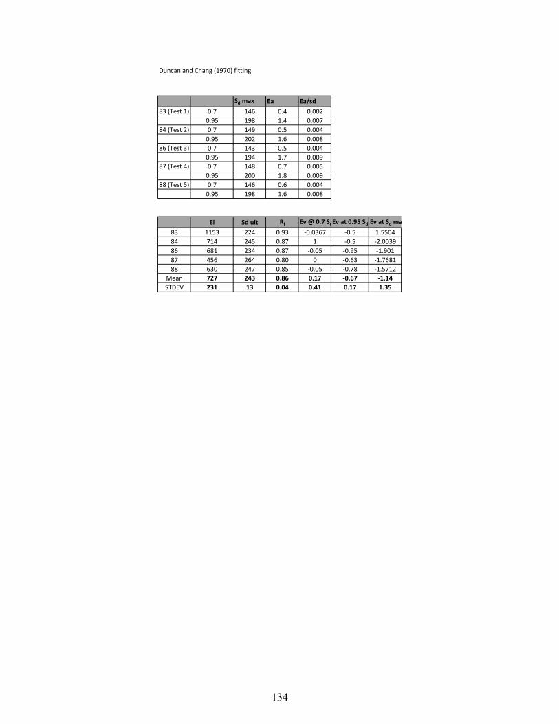
Duncan and Chang (1970) fitting
Sd max Ea Ea/sd
83 (Test 1) 0.7 146 0.4 0.002
0.95 198 1.4 0.007
84 (Test 2) 0.7 149 0.5 0.004
0.95 202 1.6 0.008
86 (Test 3) 0.7 143 0.5 0.004
0.95 194 1.7 0.009
87 (Test 4) 0.7 148 0.7 0.005
0.95 200 1.8 0.009
88 (Test 5) 0.7 146 0.6 0.004
0.95 198 1.6 0.008
Ei Sd ult Rf Ev @ 0.7 SdEv at 0.95 Sd Ev at Sd ma
83 1153 224 0.93 ‐0.0367 ‐0.5 1.5504
84 714 245 0.87 1 ‐0.5 ‐2.0039
86 681 234 0.87 ‐0.05 ‐0.95 ‐1.901
87 456 264 0.80 0 ‐0.63 ‐1.7681
88 630 247 0.85 ‐0.05 ‐0.78 ‐1.5712
Mean 727 243 0.86 0.17 ‐0.67 ‐1.14
STDEV 231 13 0.04 0.41 0.17 1.35
134

0
50
100
150
200
250
0.0
0.5
1.0
1.5
2.0
2.5
3.0
3.5
4.0
4.5
5.0
Differential Stress, Sd (kPa)
Axial Strain, Ea (%
)
Never Frozen San
d Stress‐Strain Results
1 2 3 4 5
135
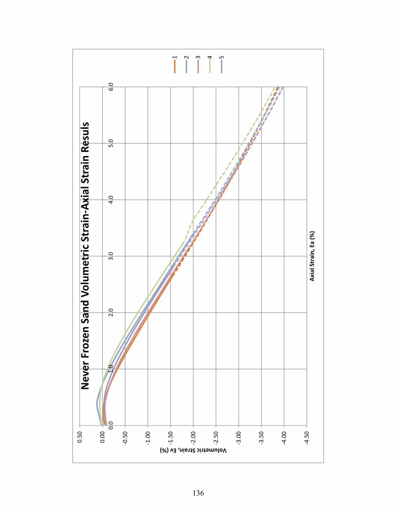
‐4.50
‐4.00
‐3.50
‐3.00
‐2.50
‐2.00
‐1.50
‐1.00
‐0.50
0.00
0.50
0.0
1.0
2.0
3.0
4.0
5.0
6.0
Volumetric Strain, Ev (%)
Axial Strain, Ea (%
)
Never Frozen San
d Volumetric Strain‐Axial Strain Resuls
1 2 3 4 5
136
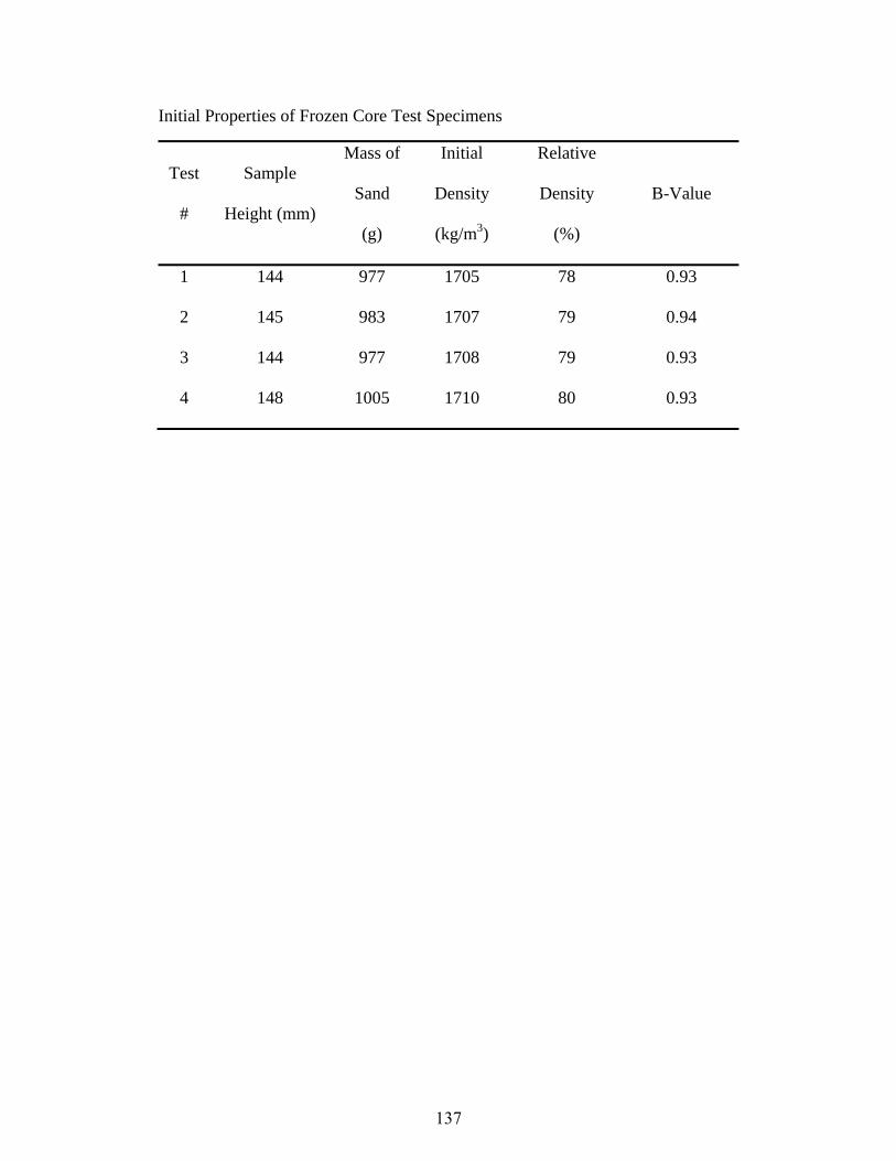
Initial Properties of Frozen Core Test Specimens
Test
#
Sample
Height (mm)
Mass of
Sand
(g)
Initial
Density
(kg/m3)
Relative
Density
(%)
B-Value
1 144 977 1705 78 0.93
2 145 983 1707 79 0.94
3 144 977 1708 79 0.93
4 148 1005 1710 80 0.93
137

Frozen/Thawed Test Data
Ea Sd Ev Sd Ev Sd Ev Sd Ev Sd Ev
0.0 0 0.00 0 0.00 0 0 0 0.00
0.1 45 0.07 36 0.09 54 40 44 0.08
0.2 81 0.12 64 0.13 85 67 74 0.13
0.3 106 0.13 87 0.16 106 90 97 0.14
0.4 130 0.11 108 0.17 121 110 117 0.14
0.5 144 0.08 120 0.16 130 126 130 0.12
0.6 158 0.04 132 0.14 139 140 142 0.09
0.7 166 ‐0.01 139 0.11 147 0.00 148 0.00 150 0.02
0.8 173 ‐0.06 145 0.07 155 ‐0.03 160 ‐0.07 158 ‐0.02
0.9 178 ‐0.12 151 0.03 162 ‐0.06 168 ‐0.15 165 ‐0.07
1.0 184 ‐0.17 156 ‐0.02 167 ‐0.10 173 ‐0.22 170 ‐0.13
1.1 188 ‐0.24 160 ‐0.07 172 ‐0.13 177 ‐0.27 174 ‐0.18
1.2 191 ‐0.31 164 ‐0.12 176 ‐0.17 182 ‐0.35 178 ‐0.24
1.3 194 ‐0.38 167 ‐0.17 180 ‐0.22 185 ‐0.42 182 ‐0.30
1.4 197 ‐0.45 170 ‐0.23 182 ‐0.27 189 ‐0.50 185 ‐0.36
1.5 199 ‐0.53 173 ‐0.29 185 ‐0.33 192 ‐0.57 187 ‐0.43
1.6 202 ‐0.60 175 ‐0.35 187 ‐0.37 195 ‐0.63 190 ‐0.49
1.7 203 ‐0.68 178 ‐0.42 189 ‐0.43 197 ‐0.71 192 ‐0.56
1.8 205 ‐0.75 180 ‐0.48 191 ‐0.49 200 ‐0.79 194 ‐0.63
1.9 206 ‐0.84 182 ‐0.55 193 ‐0.55 202 ‐0.86 195 ‐0.70
2.0 208 ‐0.91 183 ‐0.61 194 ‐0.61 203 ‐0.94 197 ‐0.77
2.1 209 ‐0.99 185 ‐0.68 195 ‐0.67 204 ‐1.00 198 ‐0.83
2.2 209 ‐1.08 186 ‐0.75 196 ‐0.73 204 ‐1.08 199 ‐0.91
2.3 210 ‐1.15 187 ‐0.81 197 ‐0.80 205 ‐1.16 200 ‐0.98
2.4 210 ‐1.24 188 ‐0.89 198 ‐0.87 205 ‐1.23 200 ‐1.06
2.5 211 ‐1.32 189 ‐0.95 199 ‐0.93 205 ‐1.31 201 ‐1.13
2.6 211 ‐1.39 190 ‐1.03 198 ‐0.99 204 ‐1.38 201 ‐1.20
2.7 212 ‐1.47 191 ‐1.10 198 ‐1.06 204 ‐1.46 201 ‐1.27
2.8 212 ‐1.55 193 ‐1.17 197 ‐1.13 204 ‐1.53 201 ‐1.35
2.9 212 ‐1.64 194 ‐1.25 197 ‐1.20 204 ‐1.61 202 ‐1.42
3.0 212 ‐1.72 194 ‐1.32 197 ‐1.27 204 ‐1.69 202 ‐1.50
3.1 213 ‐1.79 194 ‐1.40 196 ‐1.33 203 ‐1.75 202 ‐1.57
3.2 212 ‐1.88 194 ‐1.47 196 ‐1.40 203 ‐1.82 201 ‐1.64
3.3 212 ‐1.95 194 ‐1.54 196 ‐1.47 202 ‐1.90 201 ‐1.72
3.4 213 ‐2.04 194 ‐1.62 195 ‐1.54 201 ‐1.98 201 ‐1.79
3.5 212 ‐2.11 195 ‐1.69 195 ‐1.61 201 ‐2.05 201 ‐1.87
3.6 211 ‐2.20 195 ‐1.77 195 ‐1.67 200 ‐2.11 200 ‐1.94
3.7 211 ‐2.28 195 ‐1.84 194 ‐1.75 198 ‐2.19 200 ‐2.02
3.8 211 ‐2.36 195 ‐1.91 194 ‐1.82 197 ‐2.27 199 ‐2.09
3.9 210 ‐2.44 195 ‐1.99 193 ‐1.89 196 ‐2.34 199 ‐2.16
4.0 210 ‐2.52 196 ‐2.06 193 ‐1.96 195 ‐2.41 198 ‐2.24
4.1 209 ‐2.59 196 ‐2.13 193 ‐2.02 194 ‐2.47 198 ‐2.30
4.2 208 ‐2.67 196 ‐2.21 192 ‐2.09 193 ‐2.55 197 ‐2.38
4.3 208 ‐2.74 196 ‐2.27 192 ‐2.17 191 ‐2.62 197 ‐2.45
4.4 207 ‐2.82 196 ‐2.35 191 ‐2.24 189 ‐2.69 196 ‐2.53
4.5 206 ‐2.90 196 ‐2.42 191 ‐2.31 187 ‐2.76 195 ‐2.60
4.6 206 ‐2.97 196 ‐2.50 191 ‐2.37 185 ‐2.82 194 ‐2.66
4.7 205 ‐3.04 195 ‐2.57 191 ‐2.45 183 ‐2.89 194 ‐2.74
4.8 205 ‐3.11 195 ‐2.64 190 ‐2.51 181 ‐2.96 193 ‐2.80
4.9 204 ‐3.19 195 ‐2.71 190 ‐2.57 179 ‐3.03 192 ‐2.87
5.0 203 ‐3.26 195 ‐2.78 190 ‐2.64 178 ‐3.09 191 ‐2.94
3 4 Mean1 2
138
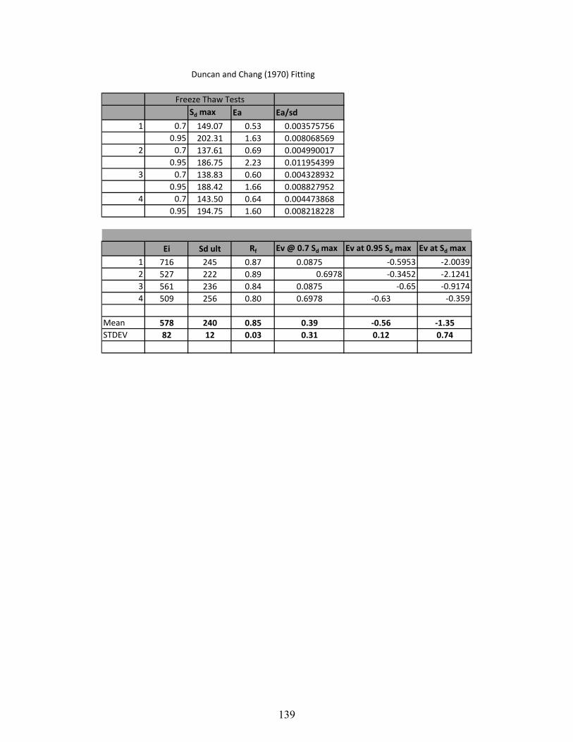
Duncan and Chang (1970) Fitting
Freeze Thaw Tests
Sd max Ea Ea/sd
1 0.7 149.07 0.53 0.003575756
0.95 202.31 1.63 0.008068569
2 0.7 137.61 0.69 0.004990017
0.95 186.75 2.23 0.011954399
3 0.7 138.83 0.60 0.004328932
0.95 188.42 1.66 0.008827952
4 0.7 143.50 0.64 0.004473868
0.95 194.75 1.60 0.008218228
Ei Sd ult Rf Ev @ 0.7 Sd max Ev at 0.95 Sd max Ev at Sd max
1 716 245 0.87 0.0875 ‐0.5953 ‐2.0039
2 527 222 0.89 0.6978 ‐0.3452 ‐2.1241
3 561 236 0.84 0.0875 ‐0.65 ‐0.9174
4 509 256 0.80 0.6978 ‐0.63 ‐0.359
Mean 578 240 0.85 0.39 ‐0.56 ‐1.35
STDEV 82 12 0.03 0.31 0.12 0.74
139

0
50
100
150
200
250
0.0
0.5
1.0
1.5
2.0
2.5
3.0
3.5
4.0
4.5
5.0
Deviator Stress, Sd (kPa)
Axial Strain, Ea (%
)
Frozen/Thaw
ed Stress‐Strain Results
1 2 3 4
140
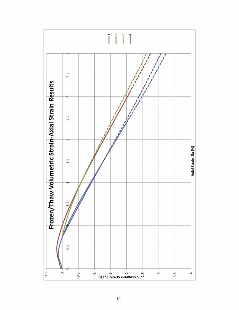
‐4
‐3.5‐3
‐2.5‐2
‐1.5‐1
‐0.50
0.5
00.5
11.5
22.5
33.5
44.5
5
Volumetric Strain, Ev (%)
Axial Strain, Ea (%
)
Frozen/Thaw
Volumetric Strain‐Axial Strain Results
1 2 3 4
141

0
50
100
150
200
250
0.0
0.5
1.0
1.5
2.0
2.5
3.0
3.5
4.0
4.5
5.0
Deviator Strain, Sd (kPa)
Axial Strain (Ea)
Mean
Stress‐Strain Results
Frozen Thaw
ed
Never Frozen
142
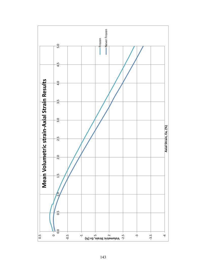
‐4
‐3.5‐3
‐2.5‐2
‐1.5‐1
‐0.50
0.5
0.0
0.5
1.0
1.5
2.0
2.5
3.0
3.5
4.0
4.5
5.0
Volumetric Strain, Ev (%)
Axial Strain, Ea, (%)
Mean
Volumetric strain‐Axial Strain Results
Frozen
Never Frozen
143
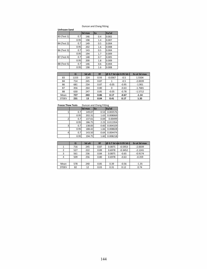
Duncan and Chang fitting
Unfrozen Sand
Sd max Ea Ea/sd
83 (Test 1) 0.7 146 0.4 0.002
0.95 198 1.4 0.007
84 (Test 2) 0.7 149 0.5 0.004
0.95 202 1.6 0.008
86 (Test 3) 0.7 143 0.5 0.004
0.95 194 1.7 0.009
87 (Test 4) 0.7 148 0.7 0.005
0.95 200 1.8 0.009
88 (Test 5) 0.7 146 0.6 0.004
0.95 198 1.6 0.008
Ei Sd ult Rf @ 0.7 Sd mat 0.95 Sd m Ev at Sd max
83 1153 224 0.93 ‐0.0367 ‐0.5 1.5504
84 714 245 0.87 1 ‐0.5 ‐2.0039
86 681 234 0.87 ‐0.05 ‐0.95 ‐1.901
87 456 264 0.80 0 ‐0.63 ‐1.7681
88 630 247 0.85 ‐0.05 ‐0.78 ‐1.5712
Mean 727 243 0.86 0.17 ‐0.67 ‐1.14
STDEV 231 13 0.04 0.41 0.17 1.35
Freeze Thaw Tests Duncan and Chang Fitting
Sd max Ea Ea/sd
1 0.7 149.07 0.53 0.003576
0.95 202.31 1.63 0.008069
2 0.7 137.61 0.69 0.00499
0.95 186.75 2.23 0.011954
3 0.7 138.83 0.60 0.004329
0.95 188.42 1.66 0.008828
4 0.7 143.50 0.64 0.004474
0.95 194.75 1.60 0.008218
Ei Sd ult Rf @ 0.7 Sd mat 0.95 Sd m Ev at Sd max
1 716 245 0.87 0.0875 ‐0.5953 ‐2.0039
2 527 222 0.89 0.6978 ‐0.3452 ‐2.1241
3 561 236 0.84 0.0875 ‐0.65 ‐0.9174
4 509 256 0.80 0.6978 ‐0.63 ‐0.359
Mean 578 240 0.85 0.39 ‐0.56 ‐1.35
STDEV 82 12 0.03 0.31 0.12 0.74
144
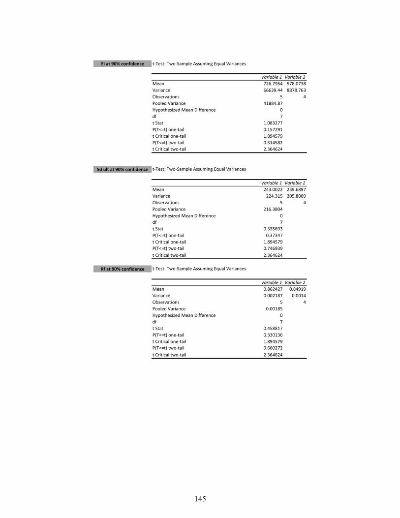
Ei at 90% confidence t‐Test: Two‐Sample Assuming Equal Variances
Variable 1 Variable 2
Mean 726.7954 578.0738
Variance 66639.44 8878.763
Observations 5 4
Pooled Variance 41884.87
Hypothesized Mean Difference 0
df 7
t Stat 1.083277
P(T<=t) one‐tail 0.157291
t Critical one‐tail 1.894579
P(T<=t) two‐tail 0.314582
t Critical two‐tail 2.364624
Sd ult at 90% confidence t‐Test: Two‐Sample Assuming Equal Variances
Variable 1 Variable 2
Mean 243.0022 239.6897
Variance 224.315 205.8009
Observations 5 4
Pooled Variance 216.3804
Hypothesized Mean Difference 0
df 7
t Stat 0.335693
P(T<=t) one‐tail 0.37347
t Critical one‐tail 1.894579
P(T<=t) two‐tail 0.746939
t Critical two‐tail 2.364624
Rf at 90% confidence t‐Test: Two‐Sample Assuming Equal Variances
Variable 1 Variable 2
Mean 0.862427 0.84919
Variance 0.002187 0.0014
Observations 5 4
Pooled Variance 0.00185
Hypothesized Mean Difference 0
df 7
t Stat 0.458817
P(T<=t) one‐tail 0.330136
t Critical one‐tail 1.894579
P(T<=t) two‐tail 0.660272
t Critical two‐tail 2.364624
145

t‐Test: Two‐Sample Assuming Equal Variances
Variable 1 Variable 2
Mean 0.17266 0.39265
Variance 0.214322 0.124155
Observations 5 4
Pooled Variance 0.175679
Hypothesized Mean Difference 0
df 7
t Stat ‐0.78241
P(T<=t) one‐tail 0.229808
t Critical one‐tail 1.894579
P(T<=t) two‐tail 0.459616
t Critical two‐tail 2.364624
t‐Test: Two‐Sample Assuming Equal Variances
Variable 1 Variable 2
Mean ‐0.672 ‐0.55513
Variance 0.03747 0.020097
Observations 5 4
Pooled Variance 0.030024
Hypothesized Mean Difference 0
df 7
t Stat ‐1.00549
P(T<=t) one‐tail 0.174072
t Critical one‐tail 1.894579
P(T<=t) two‐tail 0.348144
t Critical two‐tail 2.364624
t‐Test: Two‐Sample Assuming Equal Variances
Variable 1 Variable 2
Mean ‐1.13876 ‐1.3511
Variance 2.286033 0.732012
Observations 5 4
Pooled Variance 1.620024
Hypothesized Mean Difference 0
df 7
t Stat 0.248694
P(T<=t) one‐tail 0.405368
t Critical one‐tail 1.894579
P(T<=t) two‐tail 0.810736
t Critical two‐tail 2.364624
Ev @ 0.7 Sd max at 90%
confidence
Ev @ 0.95 Sd max at 90%
confidence
Ev @ Sd max at 90%
confidence
146

Initial Properties of Undrained Baseline Tests Specimens
Test
#
Sample
Height
(mm)
Mass of
Sand
(g)
Initial
Density
(kg/m3)
Relative
Density
(%)
B-Value
1 150 1019 1710 80 0.90
2 149 1013 1712 81 0.90
3 150 1012 1714 82 0.96
4 150 1019 1710 80 0.95
5 149 1012 1710 80 0.93
147
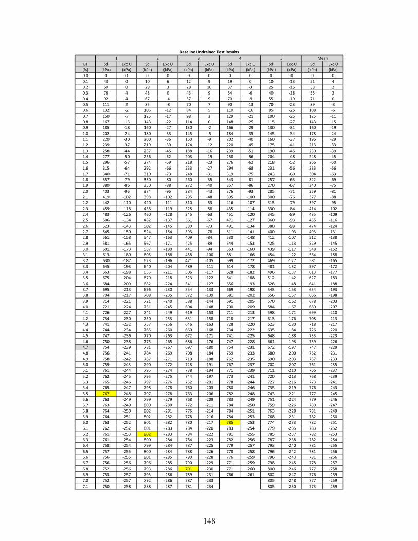
Baseline Undrained Test Results
Ea Sd Exc U Sd Exc U Sd Exc U Sd Exc U Sd Exc U Sd Exc U
(%) (kPa) (kPa) (kPa) (kPa) (kPa) (kPa) (kPa) (kPa) (kPa) (kPa) (kPa) (kPa)
0.0 0 0 0 0 0 0 0 0 0 0 0 0
0.1 43 0 10 6 12 9 19 0 10 ‐13 21 4
0.2 60 0 29 3 28 10 37 ‐3 25 ‐15 38 2
0.3 76 4 48 0 43 9 54 ‐6 40 ‐18 55 2
0.4 92 4 67 ‐4 57 9 70 ‐9 55 ‐19 71 0
0.5 111 2 85 ‐8 70 7 90 ‐13 70 ‐23 89 ‐3
0.6 132 ‐2 105 ‐12 84 5 110 ‐16 85 ‐26 108 ‐6
0.7 150 ‐7 125 ‐17 98 3 129 ‐21 100 ‐25 125 ‐11
0.8 167 ‐13 143 ‐22 114 0 148 ‐25 115 ‐27 143 ‐15
0.9 185 ‐18 160 ‐27 130 ‐2 166 ‐29 130 ‐31 160 ‐19
1.0 202 ‐24 180 ‐33 145 ‐5 184 ‐35 145 ‐34 178 ‐24
1.1 220 ‐30 200 ‐36 160 ‐9 202 ‐40 160 ‐37 196 ‐29
1.2 239 ‐37 219 ‐39 174 ‐12 220 ‐45 175 ‐41 213 ‐33
1.3 258 ‐44 237 ‐45 188 ‐16 239 ‐51 190 ‐45 230 ‐39
1.4 277 ‐50 256 ‐52 203 ‐19 258 ‐56 204 ‐48 248 ‐45
1.5 296 ‐57 274 ‐59 218 ‐23 276 ‐62 218 ‐52 266 ‐50
1.6 315 ‐64 292 ‐66 233 ‐27 294 ‐68 231 ‐56 283 ‐56
1.7 340 ‐71 310 ‐73 248 ‐31 319 ‐75 243 ‐60 304 ‐63
1.8 357 ‐79 330 ‐80 260 ‐35 343 ‐81 257 ‐63 322 ‐69
1.9 380 ‐86 350 ‐88 272 ‐40 357 ‐86 270 ‐67 340 ‐75
2.0 403 ‐95 374 ‐95 284 ‐43 376 ‐93 285 ‐71 359 ‐81
2.1 419 ‐102 398 ‐102 295 ‐48 395 ‐100 300 ‐76 377 ‐88
2.2 442 ‐110 420 ‐111 310 ‐53 416 ‐107 315 ‐79 397 ‐95
2.3 459 ‐118 438 ‐119 325 ‐58 435 ‐114 330 ‐84 414 ‐102
2.4 483 ‐126 460 ‐128 345 ‐63 451 ‐120 345 ‐89 435 ‐109
2.5 506 ‐134 482 ‐137 361 ‐67 471 ‐127 360 ‐93 455 ‐116
2.6 523 ‐143 502 ‐145 380 ‐73 491 ‐134 380 ‐98 474 ‐124
2.7 545 ‐150 524 ‐154 393 ‐78 511 ‐141 400 ‐103 493 ‐131
2.8 561 ‐158 547 ‐163 409 ‐84 530 ‐148 412 ‐107 512 ‐138
2.9 581 ‐165 567 ‐171 425 ‐89 544 ‐153 425 ‐113 529 ‐145
3.0 601 ‐173 587 ‐180 441 ‐94 563 ‐160 439 ‐117 548 ‐152
3.1 613 ‐180 605 ‐188 458 ‐100 581 ‐166 454 ‐122 564 ‐158
3.2 630 ‐187 623 ‐196 471 ‐105 599 ‐172 469 ‐127 581 ‐165
3.3 645 ‐193 640 ‐204 489 ‐111 614 ‐178 481 ‐132 597 ‐172
3.4 663 ‐198 655 ‐211 506 ‐117 628 ‐182 496 ‐137 613 ‐177
3.5 675 ‐204 670 ‐218 523 ‐122 641 ‐188 512 ‐142 627 ‐183
3.6 684 ‐209 682 ‐224 541 ‐127 656 ‐193 528 ‐148 641 ‐188
3.7 695 ‐213 696 ‐230 554 ‐133 669 ‐198 543 ‐153 654 ‐193
3.8 704 ‐217 708 ‐235 572 ‐139 681 ‐202 556 ‐157 666 ‐198
3.9 714 ‐221 721 ‐240 588 ‐144 691 ‐205 570 ‐162 678 ‐203
4.0 721 ‐224 731 ‐245 604 ‐148 700 ‐209 584 ‐167 689 ‐207
4.1 726 ‐227 741 ‐249 619 ‐153 711 ‐213 598 ‐171 699 ‐210
4.2 734 ‐230 750 ‐253 631 ‐158 718 ‐217 613 ‐176 708 ‐213
4.3 741 ‐232 757 ‐256 646 ‐163 728 ‐220 623 ‐180 718 ‐217
4.4 744 ‐234 765 ‐260 660 ‐168 734 ‐222 635 ‐184 726 ‐220
4.5 747 ‐236 770 ‐263 672 ‐171 741 ‐225 648 ‐188 733 ‐223
4.6 750 ‐238 775 ‐265 686 ‐176 747 ‐228 661 ‐193 739 ‐226
4.7 754 ‐239 781 ‐267 697 ‐180 754 ‐231 672 ‐197 747 ‐229
4.8 756 ‐241 784 ‐269 708 ‐184 759 ‐233 680 ‐200 752 ‐231
4.9 758 ‐242 787 ‐271 719 ‐188 762 ‐235 690 ‐203 757 ‐233
5.0 759 ‐243 790 ‐272 728 ‐191 767 ‐237 702 ‐207 761 ‐235
5.1 761 ‐244 795 ‐274 738 ‐194 771 ‐239 711 ‐210 766 ‐237
5.2 762 ‐245 795 ‐275 744 ‐197 773 ‐241 720 ‐213 768 ‐239
5.3 765 ‐246 797 ‐276 752 ‐201 778 ‐244 727 ‐216 773 ‐241
5.4 765 ‐247 798 ‐278 760 ‐203 780 ‐246 735 ‐219 776 ‐243
5.5 767 ‐248 797 ‐278 763 ‐206 782 ‐248 743 ‐221 777 ‐245
5.6 763 ‐249 799 ‐279 768 ‐209 783 ‐249 751 ‐224 779 ‐246
5.7 763 ‐249 800 ‐280 772 ‐211 784 ‐250 759 ‐226 780 ‐247
5.8 764 ‐250 802 ‐281 776 ‐214 784 ‐251 763 ‐228 781 ‐249
5.9 764 ‐251 802 ‐282 778 ‐216 784 ‐253 768 ‐231 782 ‐250
6.0 763 ‐252 801 ‐282 780 ‐217 785 ‐253 774 ‐233 782 ‐251
6.1 762 ‐252 801 ‐283 784 ‐220 783 ‐254 779 ‐235 783 ‐252
6.2 761 ‐253 802 ‐283 784 ‐222 781 ‐255 785 ‐237 782 ‐253
6.3 761 ‐254 800 ‐284 784 ‐223 782 ‐256 787 ‐238 782 ‐254
6.4 758 ‐254 799 ‐284 787 ‐225 779 ‐257 793 ‐240 781 ‐255
6.5 757 ‐255 800 ‐284 788 ‐226 778 ‐258 796 ‐242 781 ‐256
6.6 756 ‐255 801 ‐285 790 ‐228 776 ‐259 796 ‐243 781 ‐256
6.7 756 ‐256 796 ‐285 790 ‐229 771 ‐259 798 ‐245 778 ‐257
6.8 752 ‐256 793 ‐286 791 ‐230 771 ‐260 800 ‐246 777 ‐258
6.9 753 ‐257 795 ‐286 789 ‐231 766 ‐261 802 ‐247 776 ‐259
7.0 752 ‐257 792 ‐286 787 ‐233 805 ‐248 777 ‐259
7.1 750 ‐258 788 ‐287 781 ‐234 805 ‐250 773 ‐259
1 2 3 4 5 Mean
148

7.2 751 ‐258 787 ‐287 779 ‐235 807 ‐251 772 ‐260
7.3 751 ‐258 783 ‐287 772 ‐236 810 ‐252 769 ‐260
7.4 749 ‐259 782 ‐287 768 ‐236 812 ‐252 766 ‐261
7.5 747 ‐259 782 ‐288 762 ‐237 811 ‐253 764 ‐261
7.6 745 ‐259 777 ‐288 759 ‐238 813 ‐254 760 ‐262
7.7 743 ‐260 774 ‐288 755 ‐238 811 ‐255 757 ‐262
7.8 744 ‐260 770 ‐288 746 ‐239 809 ‐256 753 ‐263
7.9 743 ‐260 766 ‐288 742 ‐240 807 ‐256 751 ‐263
8.0 744 ‐261 763 ‐289 734 ‐240 805 ‐257 747 ‐263
8.1 744 ‐261 759 ‐289 731 ‐241 804 ‐257 745 ‐264
8.2 743 ‐261 760 ‐289 727 ‐241 805 ‐258 744 ‐264
8.3 744 ‐262 755 ‐289 725 ‐241 801 ‐258 741 ‐264
8.4 750 ‐262 752 ‐289 722 ‐242 802 ‐258 741 ‐264
8.5 748 ‐262 748 ‐289 710 ‐242 795 ‐259 735 ‐265
8.6 747 ‐262 746 ‐290 712 ‐243 793 ‐259 735 ‐265
8.7 749 ‐262 739 ‐290 708 ‐243 792 ‐259 732 ‐265
8.8 747 ‐263 737 ‐289 703 ‐243 788 ‐260 729 ‐265
8.9 745 ‐263 732 ‐289 697 ‐243 785 ‐260 725 ‐265
9.0 743 ‐263 731 ‐289 695 ‐243 779 ‐260 723 ‐265
149

0
100
200
300
400
500
600
700
800
900
01
23
45
67
89
Deviator Stress, Sd (kPa)
Axial Strain, Ea (%
)
Undrained Baselin
e Test Results
1 2 3 4 5
150
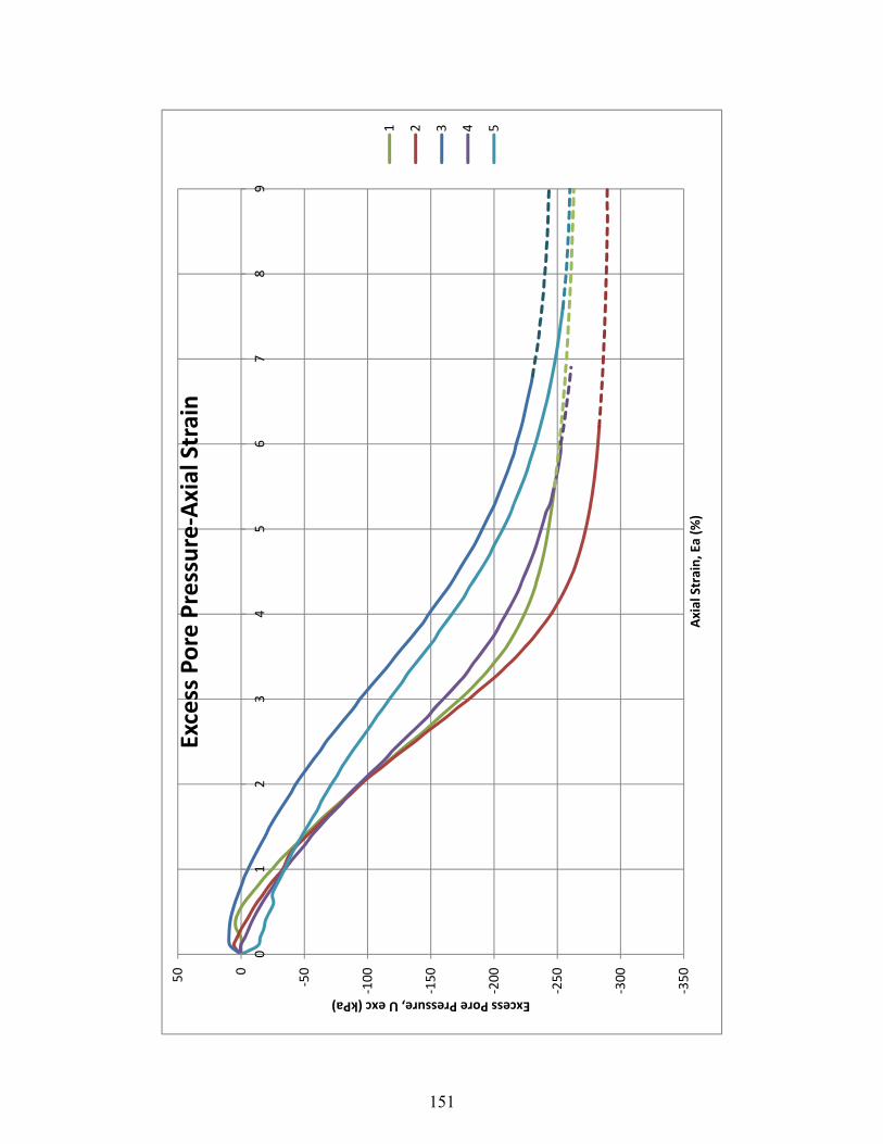
‐350
‐300
‐250
‐200
‐150
‐100
‐500
50
01
23
45
67
89
Excess Pore Pressure, U exc (kPa)
Axial Strain, Ea (%
)
Excess Pore Pressure‐Axial Strain
1 2 3 4 5
151

Initial Properties of Frozen Core Test Specimens
Test
#
Sample
Height (mm)
Mass of Sand
(g)
Initial Density
(kg/m3)
Relative
Density
(%)
B-
Value
1 150 1020 1711 80 0.90
2 145 985 1708 79 0.93
3 144 979 1710 80 0.90
152
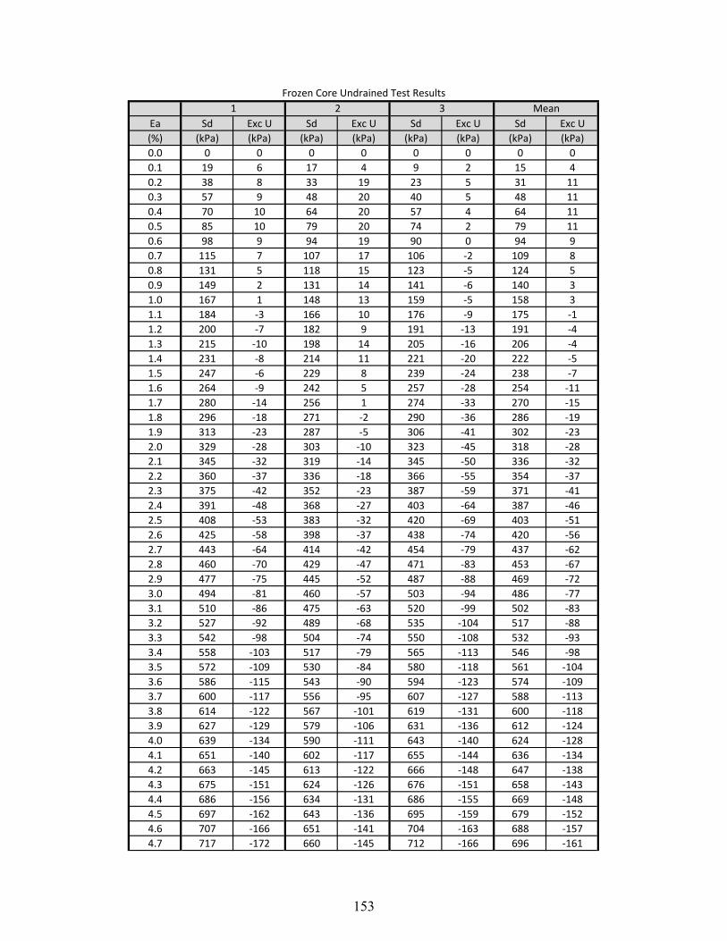
Frozen Core Undrained Test Results
Ea Sd Exc U Sd Exc U Sd Exc U Sd Exc U
(%) (kPa) (kPa) (kPa) (kPa) (kPa) (kPa) (kPa) (kPa)
0.0 0 0 0 0 0 0 0 0
0.1 19 6 17 4 9 2 15 4
0.2 38 8 33 19 23 5 31 11
0.3 57 9 48 20 40 5 48 11
0.4 70 10 64 20 57 4 64 11
0.5 85 10 79 20 74 2 79 11
0.6 98 9 94 19 90 0 94 9
0.7 115 7 107 17 106 ‐2 109 8
0.8 131 5 118 15 123 ‐5 124 5
0.9 149 2 131 14 141 ‐6 140 3
1.0 167 1 148 13 159 ‐5 158 3
1.1 184 ‐3 166 10 176 ‐9 175 ‐1
1.2 200 ‐7 182 9 191 ‐13 191 ‐4
1.3 215 ‐10 198 14 205 ‐16 206 ‐4
1.4 231 ‐8 214 11 221 ‐20 222 ‐5
1.5 247 ‐6 229 8 239 ‐24 238 ‐7
1.6 264 ‐9 242 5 257 ‐28 254 ‐11
1.7 280 ‐14 256 1 274 ‐33 270 ‐15
1.8 296 ‐18 271 ‐2 290 ‐36 286 ‐19
1.9 313 ‐23 287 ‐5 306 ‐41 302 ‐23
2.0 329 ‐28 303 ‐10 323 ‐45 318 ‐28
2.1 345 ‐32 319 ‐14 345 ‐50 336 ‐32
2.2 360 ‐37 336 ‐18 366 ‐55 354 ‐37
2.3 375 ‐42 352 ‐23 387 ‐59 371 ‐41
2.4 391 ‐48 368 ‐27 403 ‐64 387 ‐46
2.5 408 ‐53 383 ‐32 420 ‐69 403 ‐51
2.6 425 ‐58 398 ‐37 438 ‐74 420 ‐56
2.7 443 ‐64 414 ‐42 454 ‐79 437 ‐62
2.8 460 ‐70 429 ‐47 471 ‐83 453 ‐67
2.9 477 ‐75 445 ‐52 487 ‐88 469 ‐72
3.0 494 ‐81 460 ‐57 503 ‐94 486 ‐77
3.1 510 ‐86 475 ‐63 520 ‐99 502 ‐83
3.2 527 ‐92 489 ‐68 535 ‐104 517 ‐88
3.3 542 ‐98 504 ‐74 550 ‐108 532 ‐93
3.4 558 ‐103 517 ‐79 565 ‐113 546 ‐98
3.5 572 ‐109 530 ‐84 580 ‐118 561 ‐104
3.6 586 ‐115 543 ‐90 594 ‐123 574 ‐109
3.7 600 ‐117 556 ‐95 607 ‐127 588 ‐113
3.8 614 ‐122 567 ‐101 619 ‐131 600 ‐118
3.9 627 ‐129 579 ‐106 631 ‐136 612 ‐124
4.0 639 ‐134 590 ‐111 643 ‐140 624 ‐128
4.1 651 ‐140 602 ‐117 655 ‐144 636 ‐134
4.2 663 ‐145 613 ‐122 666 ‐148 647 ‐138
4.3 675 ‐151 624 ‐126 676 ‐151 658 ‐143
4.4 686 ‐156 634 ‐131 686 ‐155 669 ‐148
4.5 697 ‐162 643 ‐136 695 ‐159 679 ‐152
4.6 707 ‐166 651 ‐141 704 ‐163 688 ‐157
4.7 717 ‐172 660 ‐145 712 ‐166 696 ‐161
1 2 3 Mean
153

4.8 726 ‐176 668 ‐150 720 ‐169 704 ‐165
4.9 734 ‐181 675 ‐154 727 ‐172 712 ‐169
5.0 741 ‐186 682 ‐158 734 ‐175 719 ‐173
5.1 748 ‐190 688 ‐162 740 ‐178 726 ‐177
5.2 754 ‐195 695 ‐166 746 ‐181 732 ‐180
5.3 761 ‐199 700 ‐170 751 ‐183 737 ‐184
5.4 767 ‐203 706 ‐173 756 ‐185 743 ‐187
5.5 772 ‐207 711 ‐177 761 ‐188 748 ‐191
5.6 777 ‐210 716 ‐180 765 ‐190 753 ‐194
5.7 781 ‐214 719 ‐184 768 ‐193 756 ‐197
5.8 786 ‐217 722 ‐187 772 ‐194 760 ‐200
5.9 791 ‐221 725 ‐190 774 ‐197 763 ‐202
6.0 795 ‐224 728 ‐193 776 ‐199 767 ‐205
6.1 800 ‐227 731 ‐196 778 ‐201 770 ‐208
6.2 803 ‐230 732 ‐198 779 ‐202 772 ‐210
6.3 807 ‐233 734 ‐201 781 ‐203 774 ‐212
6.4 810 ‐235 735 ‐204 782 ‐205 775 ‐215
6.5 813 ‐238 737 ‐206 783 ‐207 778 ‐217
6.6 816 ‐241 739 ‐209 785 ‐208 780 ‐219
6.7 818 ‐243 741 ‐211 782 ‐209 781 ‐221
6.8 820 ‐246 741 ‐213 782 ‐210 781 ‐223
6.9 822 ‐248 740 ‐215 781 ‐212 781 ‐225
7.0 824 ‐249 739 ‐217 785 ‐212 783 ‐226
7.1 825 ‐251 737 ‐219 786 ‐213 783 ‐228
7.2 826 ‐253 734 ‐221 787 ‐214 782 ‐229
7.3 827 ‐255 732 ‐223 787 ‐215 782 ‐231
7.4 829 ‐257 727 ‐224 787 ‐217 781 ‐233
7.5 830 ‐259 724 ‐226 786 ‐218 780 ‐234
7.6 830 ‐261 720 ‐228 785 ‐219 778 ‐236
7.7 830 ‐263 717 ‐229 784 ‐221 777 ‐238
7.8 829 ‐266 713 ‐231 784 ‐221 775 ‐239
7.9 831 ‐266 708 ‐232 782 ‐222 774 ‐240
8.0 831 ‐267 704 ‐233 780 ‐222 772 ‐241
8.1 830 ‐267 700 ‐235 776 ‐223 769 ‐242
8.2 828 ‐270 695 ‐236 772 ‐224 765 ‐243
8.3 825 ‐271 690 ‐237 769 ‐226 761 ‐244
8.4 823 ‐272 684 ‐238 766 ‐226 757 ‐245
8.5 820 ‐274 678 ‐239 763 ‐226 754 ‐246
8.6 817 ‐276 674 ‐240 760 ‐227 750 ‐247
8.7 814 ‐277 668 ‐241 758 ‐227 747 ‐248
8.8 810 ‐278 666 ‐242 756 ‐228 744 ‐249
8.9 806 ‐279 663 ‐243 753 ‐229 741 ‐250
9.0 804 ‐280 663 ‐244 751 ‐229 739 ‐251
154
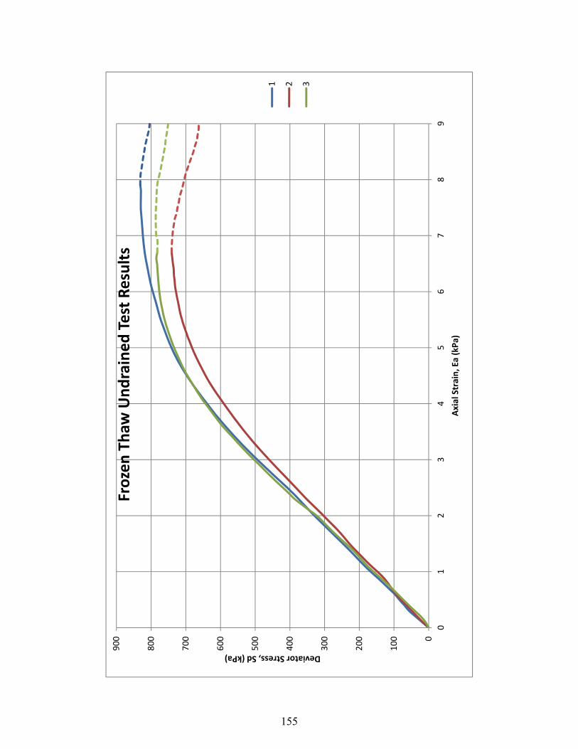
0
100
200
300
400
500
600
700
800
900
01
23
45
67
89
Deviator Stress, Sd (kPa)
Axial Strain, Ea (kPa)
Frozen Thaw
Undrained Test Results
1 2 3
155

‐300
‐250
‐200
‐150
‐100
‐500
50
01
23
45
67
89
Excess Pore Pressure , Uexc(kPa)
Axial Strain, Ea (%
)
Excess Pore Pressure‐Strain Results (Frozen Thaw
)
1 2 3
156
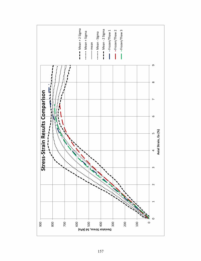
0
100
200
300
400
500
600
700
800
900
01
23
45
67
89
Deviator Stress, Sd (kPa)
Axial Strain, Ea (%
)
Stress‐Strain Results Comparison
Mean + 2 Sigma
Mean + Sigma
mean
Mean ‐ Sigma
Mean ‐ 2 Sigma
Frozen/Thaw
1
Frozen/Thaw
2
Frozen/Thaw
3
157

‐350
‐300
‐250
‐200
‐150
‐100
‐500
50
01
23
45
67
89
Excess Pore Pressure, Uexc (kPa)
Axial Strain, Ea (%
)
Excess Pore Pressure Comparison
Mean + 2 Sigma
Mean + Sigma
mean
Mean ‐ Sigma
Mean ‐ 2 Sigma
Frozen/Thaw
1
Frozen/Thaw
2
Frozen/Thaw
3
158

Stress‐Strain Curves Comparison
Excess pore water pressure, Uexc
Unfrozen sand Frozen
Test Number 1 2 3 4 5 Mean 1 2 3 Mean
1% 202 180 145 184 145 171 167 148 159 158
3% 601 587 441 563 439 526 494 460 503 486
5% 759 790 728 767 702 749 741 682 734 719
Axial strain, Ea
159
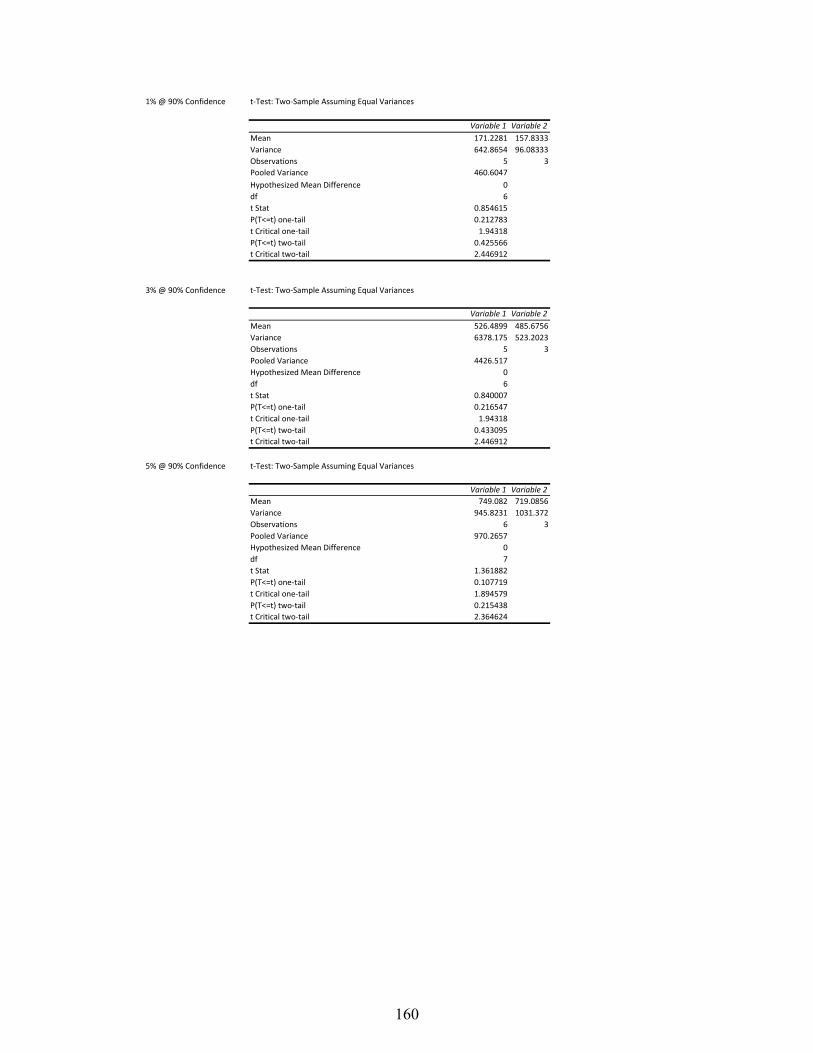
1% @ 90% Confidence t‐Test: Two‐Sample Assuming Equal Variances
Variable 1 Variable 2
Mean 171.2281 157.8333
Variance 642.8654 96.08333
Observations 5 3
Pooled Variance 460.6047
Hypothesized Mean Difference 0
df 6
t Stat 0.854615
P(T<=t) one‐tail 0.212783
t Critical one‐tail 1.94318
P(T<=t) two‐tail 0.425566
t Critical two‐tail 2.446912
3% @ 90% Confidence t‐Test: Two‐Sample Assuming Equal Variances
Variable 1 Variable 2
Mean 526.4899 485.6756
Variance 6378.175 523.2023
Observations 5 3
Pooled Variance 4426.517
Hypothesized Mean Difference 0
df 6
t Stat 0.840007
P(T<=t) one‐tail 0.216547
t Critical one‐tail 1.94318
P(T<=t) two‐tail 0.433095
t Critical two‐tail 2.446912
5% @ 90% Confidence t‐Test: Two‐Sample Assuming Equal Variances
Variable 1 Variable 2
Mean 749.082 719.0856
Variance 945.8231 1031.372
Observations 6 3
Pooled Variance 970.2657
Hypothesized Mean Difference 0
df 7
t Stat 1.361882
P(T<=t) one‐tail 0.107719
t Critical one‐tail 1.894579
P(T<=t) two‐tail 0.215438
t Critical two‐tail 2.364624
160

Excess pore water pressure comparison
Excess pore water pressure, Uexc
Unfrozen sand Frozen
Test Number 1 2 3 4 5 Mean 1 2 3 Mean
1% ‐24 ‐33 ‐5 ‐35 ‐34 ‐26 1 13 ‐5 3
3% ‐173 ‐180 ‐94 ‐160 ‐117 ‐145 ‐81 ‐57 ‐94 ‐77
5% ‐243 ‐272 ‐191 ‐237 ‐207 ‐230 ‐186 ‐158 ‐175 ‐173
Axial strain, Ea
161

t‐Test: Two‐Sample Assuming Equal Variances
1% @ 90% Confidence
Variable 1 Variable 2
Mean ‐26.344 2.89
Variance 153.1605 78.4561
Observations 5 3
Pooled Variance 128.259
Hypothesized Mean Difference 0
df 6
t Stat ‐3.53464
P(T<=t) one‐tail 0.006149
t Critical one‐tail 1.94318
P(T<=t) two‐tail 0.012298
t Critical two‐tail 2.446912
3% @ 90 % confidence t‐Test: Two‐Sample Assuming Equal Variances
Variable 1 Variable 2
Mean ‐144.808 ‐77.28
Variance 1407.177 335.6899
Observations 5 3
Pooled Variance 1050.015
Hypothesized Mean Difference 0
df 6
t Stat ‐2.85356
P(T<=t) one‐tail 0.014523
t Critical one‐tail 1.94318
P(T<=t) two‐tail 0.029046
t Critical two‐tail 2.446912
5% @ 90 % confidence t‐Test: Two‐Sample Assuming Equal Variances
Variable 1 Variable 2
Mean ‐230.046 ‐172.917
Variance 1023.825 194.1294
Observations 5 3
Pooled Variance 747.26
Hypothesized Mean Difference 0
df 6
t Stat ‐2.8617
P(T<=t) one‐tail 0.014369
t Critical one‐tail 2.446912
P(T<=t) two‐tail 0.028738
t Critical two‐tail 2.968687
t‐Test: Two‐Sample Assuming Equal Variances
1% @ 95 % confidence Variable 1 Variable 2
Mean ‐26.344 2.89
Variance 153.1605 78.4561
Observations 5 3
Pooled Variance 128.259
Hypothesized Mean Difference 0
df 6
t Stat ‐3.53464
P(T<=t) one‐tail 0.006149
t Critical one‐tail 2.446912
P(T<=t) two‐tail 0.012298
t Critical two‐tail 2.968687
162