Policy Research Working Paper 8159

Understanding the Interactions between Emissions Trading Systems and Renewable Energy Standards

Using a Multi-Regional CGE Model of ChinaYing FanJie Wu

Govinda TimilsinaYan Xia

Development Research GroupEnvironment and Energy TeamAugust 2017

WPS8159P

ublic

Dis

clos

ure

Aut

horiz

edP

ublic

Dis

clos

ure

Aut

horiz

edP

ublic

Dis

clos

ure

Aut

horiz

edP

ublic

Dis

clos

ure

Aut

horiz

ed

Produced by the Research Support Team

Abstract

The Policy Research Working Paper Series disseminates the findings of work in progress to encourage the exchange of ideas about development issues. An objective of the series is to get the findings out quickly, even if the presentations are less than fully polished. The papers carry the names of the authors and should be cited accordingly. The findings, interpretations, and conclusions expressed in this paper are entirely those of the authors. They do not necessarily represent the views of the International Bank for Reconstruction and Development/World Bank and its affiliated organizations, or those of the Executive Directors of the World Bank or the governments they represent.

Policy Research Working Paper 8159

This paper is a product of the Environment and Energy Team, Development Research Group. It is part of a larger effort by the World Bank to provide open access to its research and make a contribution to development policy discussions around the world. Policy Research Working Papers are also posted on the Web at http://econ.worldbank.org. The authors may be contacted at gtimilsina@worldbank.org.

Many countries have introduced policy measures, such as carbon pricing, greenhouse gas offsetting mecha-nisms, renewable energy standards, and energy efficiency improvements, to achieve their climate change mitigation targets. However, in many instances, these measures over-lap in ways that may dilute each policy’s greenhouse gas reduction potential. This study examines how a renewable energy standard in the power sector would interact with a national emission trading scheme that is introduced to achieve a greenhouse gas mitigation target. Using a static,

multiregional computable general equilibrium model of China to simulate policy measures, the study finds that the addition of a separate renewable energy standard policy would increase the economic cost for achieving a target level of greenhouse gas mitigation. The study con-cludes that although renewable energy standard policies promote the use of renewable energies, they are an eco-nomic burden from the perspective of reducing greenhouse gas emissions if a carbon pricing mechanism is in place.

Understanding the Interactions between Emissions Trading Systems and Renewable Energy Standards Using a Multi-Regional CGE Model of China1

Ying Fan, Jie Wu, Govinda Timilsina, Yan Xia2

Keywords: emissions trading scheme, renewable energy standards, CGE model;

climate change mitigation, China

JEL Classifications: D58, Q54

1 The authors would like to thank Cuihong Yang, Jing Cao, Bekele Debele, Garo Batmanian, Todd M. Johnson, Dafei Huang and Mike Toman for their valuable comments and suggestions. The views and interpretations are of authors and should not be attributed to the World Bank Group and the organizations they are affiliated with. We acknowledge World Bank’s Knowledge for Change (KCP) Trust Fund. 2 Ying Fan is a Professor at Beihang University, Beijing; Jie Wu is an Assistant Professor at Shanghai University of Finance and Economics; Govinda Timilsina is a Senior Economist at the Research Department of the World Bank, Washington, DC and Yan Xia is researcher at Chinese Academy of Sciences, Beijing.

2

1. Introduction

Different policy instruments are being introduced in both developed and

developing countries for greenhouse gas (GHG) mitigation. Initially, GHG mitigation

options such as energy technology mandates (e.g., renewable energy utilization

requirements) and energy efficiency standards were the focus under climate change

mitigation initiatives. While various policy options including fiscal incentives and

regulatory mandates now are common in both developed and developing countries to

promote lower-carbon energy use and efficient consumption of energy, market based

mechanisms for climate change mitigation, such as the clean development mechanism

(CDM) and other GHG offset mechanisms, also played a crucial role in the deployment

of these measures. More recently, particularly after the Paris Agreement, carbon pricing

has emerged as a key policy instrument in several countries, including developing

countries, to achieve their nationally determined commitment (NDC) agreed in the

Paris Agreement.

One issue often raised by policy makers is how to address the economic burden to

tax payers that could arise due to potential overlapping of various policy options. This

issue arises when multiple policies (e.g., carbon pricing, renewable energy mandates

and energy efficiency standards) are implemented at the same time. This study aims to

address that question in the context of energy and GHG mitigation policies in China.

Like other countries, China has proposed various policy options to meet its NDC,

including a national emission trading system (ETS) and a mandate for use of non-fossil

3

fuels to meet a given fraction (20%) of the total primary energy supply.3 While the

national ETS is expected to be introduced in 2017, renewable energy standards (RES)

policies are already in place since 2006. The ETS has been already tested through seven

pilot schemes at the provincial and city levels since 2013.

A rich literature exists on the design issues of both ETS and RES separately (see

e.g., Lesser and Su, 2008; Langniß et al., 2009; Couture and Gagnon, 2010;

Schallenberg-Rodriguez and Haas, 2012; Hübler et al., 2014; Ouyang and Lin, 2014;

He et al., 2015). Understanding of interactions between these measures also is critical

for the successful implementation of each policy.

Applying a theoretical model to understand the interactions between emissions

trading and other policy instruments, Fankhauser et al. (2010) argue that renewable

energy obligations within a capped area might have undermined the carbon price and

increased the mitigation costs. Using a partial equilibrium model to explore the

interactions between emission trading and three renewable electricity support schemes,

Böhringer and Behrens (2015) suggest that policy makers should address the

implications of the overlap between emission caps and different RES policy

instruments. Using a CGE model to analyze the interactions between a renewable

portfolio standard and a cap-and-trade policy in the United States, Morris (2009) finds

that the renewable energy portfolio increased the welfare costs of cap-and-trade policy.

Some studies blamed the renewable energy mandate in the EU for causing the

plummeting of CO2 permits prices under the EU ETS between 2008 and 2013, because

3 China has set a target of reducing its emission intensities 60% to 65% below its 2005 level by 2030; it has also planned to supply 20% of total energy consumption in 2030 from non-fossil fuel sources.

4

the mandate curtailed the demand for CO2 permits (Van den Bergh et al., 2013; Weigt

et al., 2013). Examining the relationship between the EU-ETS permit price drop and

renewable policies in the EU, Koch et al. (2014) finds that the growth of wind and solar

power generation under the EU mandate robustly explains the EU-ETS permit price

dynamics.

Some literature (Nordhaus,2011; Böhringer et al., 2009; Tsao et al., 2011; Morris,

2009) also suggests that a separate renewable energy mandate might adversely affect

low carbon economic development that could be encouraged by broader carbon pricing

policies. This is because favoring a particular technology (here renewable energy)

would depress the carbon price and associated investments on other lower carbon

technologies. For example, Nordhaus (2011) argues that depressed carbon prices caused

by the additional RES policy are not likely to provide sufficient incentives for

investments in low-carbon technologies. Newell (2015) stresses technology policies,

such as renewable portfolio standards, could raise rather than lower the societal costs

of climate mitigation; on the other hand, carbon pricing policies, such as a carbon tax

with part of the tax revenue recycled to research and development of clean technologies,

would be the most cost efficient option for climate change mitigation.

One could argue that adoption of clean and renewable energy would not only help

reduce GHG emissions, they would have other benefits, such reduction of local air

pollution. If the benefits from local air pollution are quantified and accounted for in the

analysis, it might be possible that a policy that considers both emission trading and

renewable portfolio standards simultaneously is more economic as compared to an

5

emission trading scheme alone. However, quantification of air pollution benefits is

complex and accounting for these intangible benefits in a social accounting matrix, the

main database for a CGE model is further complicated.

Against this background, our paper uses a static, multi-regional CGE model to

analyze the interactions between ETS and RES policies in China by comparing their

economywide impacts both at national and provincial levels. We simulated three cases:

(i) a base case in the absence of the ETS and RES policies; (ii) an ETS case which

considers a national emission trading scheme to reduce national CO2 emissions by 10%

from the base case; and (iii) an ETS-cum-RES case where a separate RES policy is

introduced on top of the ETS to achieve the same level of emission reduction target.

Our simulation results show that an additional RES policy would further reduce GDP

and increase the welfare loss associated with the ETS.

The paper is organized as follows. Section 2 describes the CGE model used, and

how ETS and RES policies are implemented in this model. Section 3 presents the data

and policy scenarios. Section 4 presents the economy-wide implications effects of ETS

alone and in combination with RES. Finally, key conclusions are drawn in Section 5.

2. Methodology

This research is implemented in the CEEP Multi-Regional Energy-Environment-

Economy Modelling System (CE3MS), which is based on a multi-regional static CGE

model for China (Wu et al., 2016). The CE3MS includes 30 regions in accordance with

the administrative structure of mainland China (excluding Tibet due to a lack of data).

6

Each region has independent institutions as production sectors, rural and urban

households, a representative enterprise, and a local government; and, meanwhile, has

relevant economic activities such as production, consumption, savings, and investment.

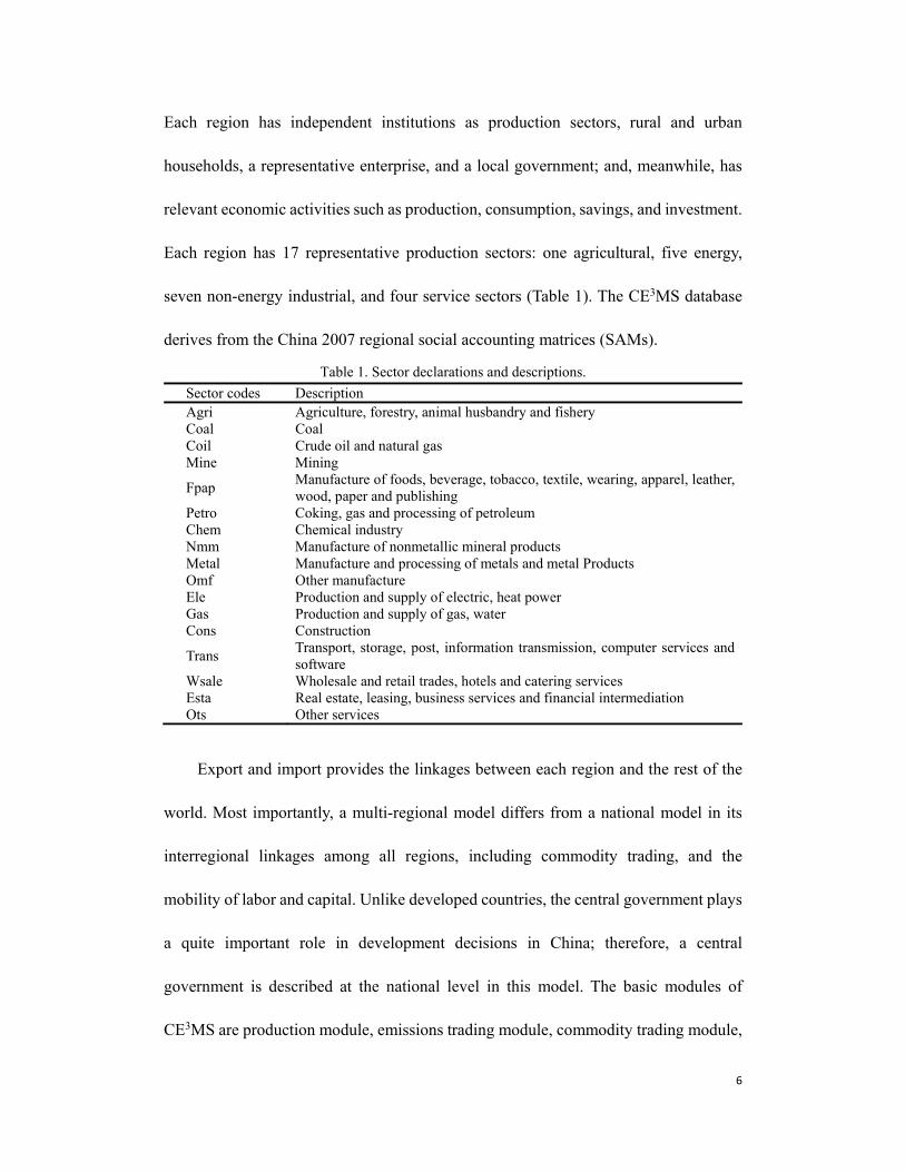
Each region has 17 representative production sectors: one agricultural, five energy,

seven non-energy industrial, and four service sectors (Table 1). The CE3MS database

derives from the China 2007 regional social accounting matrices (SAMs).

Table 1. Sector declarations and descriptions.

Sector codes Description Agri Agriculture, forestry, animal husbandry and fishery Coal Coal Coil Crude oil and natural gas Mine Mining

Fpap Manufacture of foods, beverage, tobacco, textile, wearing, apparel, leather, wood, paper and publishing

Petro Coking, gas and processing of petroleum Chem Chemical industry Nmm Manufacture of nonmetallic mineral products Metal Manufacture and processing of metals and metal Products Omf Other manufacture Ele Production and supply of electric, heat power Gas Production and supply of gas, water Cons Construction

Trans Transport, storage, post, information transmission, computer services and software

Wsale Wholesale and retail trades, hotels and catering services Esta Real estate, leasing, business services and financial intermediation Ots Other services

Export and import provides the linkages between each region and the rest of the

world. Most importantly, a multi-regional model differs from a national model in its

interregional linkages among all regions, including commodity trading, and the

mobility of labor and capital. Unlike developed countries, the central government plays

a quite important role in development decisions in China; therefore, a central

government is described at the national level in this model. The basic modules of

CE3MS are production module, emissions trading module, commodity trading module,

7

institution module, labor mobility module, and macro closure, of which the key features

are outlined below.

2.1 Production module

The model assumes that all sectors are characterized by constant returns to scale

and are traded in perfectly competitive markets. Constant elasticity of substitution

(CES) functions and nesting structures are used to characterize the production

technologies for all sectors. In the production of non-electricity sectors, energy is

treated as a special resource rather than an intermediate input and is combined with

value-added. Thus, energy can be substituted by other energy or intermediate input.

, , ,

1

, , , , , ,1j r j r j rj r j r j r j r j r j rQA QVAE QINTA (1)

,1

, , ,

, , ,1

j r

j r j r j r

j r j r j r

PVAE QINTA

PINTA QVAE

(2)

, , , , , ,j r j r j r j r j r j rPA QA PVAE QVAE PINTA QINTA (3)

where ,j rPA and ,j rQA are the producer price and output of sector j in region r,

,j rPINTA and ,j rQINTA are the price and quantity of intermediate input, ,j rPVAE

and ,j rQVAE are the price and quantity of value added and energy input. ,j r and ,j r

are the efficiency parameter and share parameter of the CES function, and ,j r is the

substitution elasticity parameter. The combination of intermediate input is presented by

Leontief functions as Equation 4 and Equation 5:

, , , , ,i j r i j r j rQINT ica QINTA (4)

, , , ,j r i j r i ri

PINTA ica PQ (5)

where , ,i j rQINT is the quantity of commodity i as intermediate input of sector j in

region r, ,i rPQ is the price of commodity i in region r, , ,i j rica is the coefficient of

8

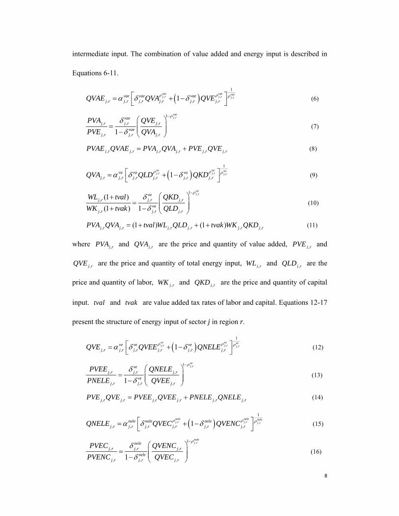
intermediate input. The combination of value added and energy input is described in

Equations 6-11.

, , ,

1

, , , , , ,1vae vae vaej r j r j rvae vae vae

j r j r j r j r j r j rQVAE QVA QVE

(6)

,1

, , ,

, , ,1

vaej rvae

j r j r j r

vaej r j r j r

PVA QVE

PVE QVA

(7)

, , , , , ,j r j r j r j r j r j rPVAE QVAE PVA QVA PVE QVE

(8)

, , ,

1

, , , , , ,1va va vaj r j r j rva va va

j r j r j r j r j r j rQVA QLD QKD

(9)

,1

, , ,

, , ,

(1 )

(1 ) 1

vaj rva

j r j r j r

vaj r j r j r

WL tval QKD

WK tvak QLD

(10)

, , , , , ,(1 ) (1 )j r j r j r j r j r j rPVA QVA tval WL QLD tvak WK QKD (11)

where ,j rPVA and ,j rQVA are the price and quantity of value added, ,j rPVE and

,j rQVE are the price and quantity of total energy input, ,j rWL and ,j rQLD are the

price and quantity of labor, ,j rWK and ,j rQKD are the price and quantity of capital

input. tval and tvak are value added tax rates of labor and capital. Equations 12-17

present the structure of energy input of sector j in region r.

, , ,

1

, , , , , ,1ve ve vej r j r j rve ve ve

j r j r j r j r j r j rQVE QVEE QNELE

(12)

,1

, , ,

, , ,1

vej rve

j r j r j r

vej r j r j r

PVEE QNELE

PNELE QVEE

(13)

, , , , , ,j r j r j r j r j r j rPVE QVE PVEE QVEE PNELE QNELE

(14)

, , ,

1

, , , , , ,1nele nele nelej r j r j rnele nele nele

j r j r j r j r j r j rQNELE QVEC QVENC

(15)

,1

, , ,

, , ,1

nelej rnele

j r j r j r

nelej r j r j r

PVEC QVENC

PVENC QVEC

(16)

9

, , , , , ,j r j r j r j r j r j rPNELE QNELE PVEC QVEC PVENC QVENC

(17)

where ,j rPVEE and ,j rQVEE are the price and quantity of electricity input,

,j rPNELE and ,j rQNELE are the price and quantity of non-electricity input.

,j rQVEC , ,j rPVEC , ,j rQVENC , ,j rPVENC are the coal input and non-coal input and

the corresponding prices, respectively.

To implement the RES policy in CE3MS, electric power generation is represented

by eight generation technologies: coal (Coa), natural gas (Ngs), petroleum (Pet),

nuclear (Nuc), hydropower (Hyd), wind (Win), solar (Sol), and other renewable

technologies (Oth). The structure of electricity production is given in Figure 1. In

particular, coal, natural gas, and petroleum are raw material inputs of coal-, natural gas-,

and petroleum-powered generation and thus are considered as intermediate inputs

rather than value-added or energy inputs for coal-, natural gas-, and petroleum-powered

generation.

Figure 1. Structure of electricity production

The total electricity output aggregation shows imperfect substitution of electricity

from different generation technologies, which reflects the reality that various power

Intermediate input

Nuclear power

Natural gas-powered

Non-energy input

Electricity

Coal-powered

Other

CES

Petroleum-powered

Hydropower

Wind power

Solar

Leontief

CES

Value-added energy

Intermediate input

CES

Value addedEnergy

Capital LabourElectricity Gas

CES

CES

Petroleum Non-energy input

Leontief

CES

Value-added energy

CES

Value addedEnergy

Capital LabourElectricity Gas

CES

CES

10

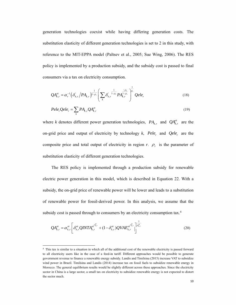
generation technologies coexist while having differing generation costs. The

substitution elasticity of different generation technologies is set to 2 in this study, with

reference to the MIT-EPPA model (Paltsev et al., 2005; Sue Wing, 2006). The RES

policy is implemented by a production subsidy, and the subsidy cost is passed to final

consumers via a tax on electricity consumption.

1

111 11 ' '1

, , , , ,

r r

r rretk r r k r k r k r k r r

k

QA PA PA Qele

(18)

, ,et

r r k r k rk

Pele Qele PA QA

(19)

where k denotes different power generation technologies, ,k rPA and ,etk rQA are the

on-grid price and output of electricity by technology k, rPele and rQele are the

composite price and total output of electricity in region r. r is the parameter of

substitution elasticity of different generation technologies.

The RES policy is implemented through a production subsidy for renewable

electric power generation in this model, which is described in Equation 22. With a

subsidy, the on-grid price of renewable power will be lower and leads to a substitution

of renewable power for fossil-derived power. In this analysis, we assume that the

subsidy cost is passed through to consumers by an electricity consumption tax.4

, , ,

1

, , , , , ,(1 )et et etk r k r k ret et et et et et

k r k r k r k r k r k rQA QINTA QVAE

(20)

4 This tax is similar to a situation in which all of the additional cost of the renewable electricity is passed forward to all electricity users like in the case of a feed-in tariff. Different approaches would be possible to generate government revenue to finance a renewable energy subsidy. Landis and Timilsina (2015) increase VAT to subsidize wind power in Brazil. Timilsina and Landis (2014) increase tax on fossil fuels to subsidize renewable energy in Morocco. The general equilibrium results would be slightly different across these approaches. Since the electricity sector in China is a large sector, a small tax on electricity to subsidize renewable energy is not expected to distort the sector much.

11

, , , , , ,et et et et et

k r k r k r k r k r k rPP QA PINTA QINTA PVAE QVAE

(21)

,, , , ,

1k r

k rsub

PPPA k Win Sol Oth

r

(22)

, ,,

, , ,sub k r k r tax r rk r r

r PA QA r Pele Qele k Win Sol Oth (23)

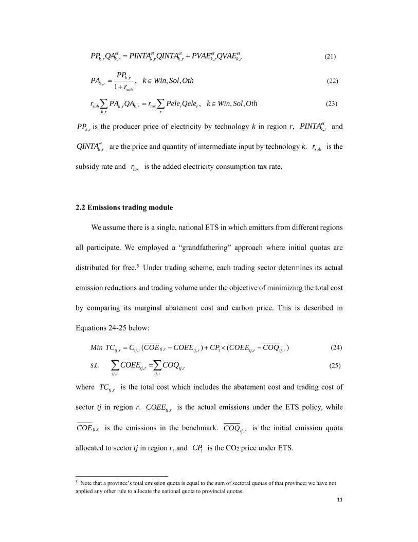
,k rPP is the producer price of electricity by technology k in region r, ,etk rPINTA and

,etk rQINTA are the price and quantity of intermediate input by technology k. subr is the

subsidy rate and taxr is the added electricity consumption tax rate.

2.2 Emissions trading module

We assume there is a single, national ETS in which emitters from different regions

all participate. We employed a “grandfathering” approach where initial quotas are

distributed for free.5 Under trading scheme, each trading sector determines its actual

emission reductions and trading volume under the objective of minimizing the total cost

by comparing its marginal abatement cost and carbon price. This is described in

Equations 24-25 below:

,, , , 1 , ,( ) ( )tj rtj r tj r tj r tj r tj rMin TC C COE COEE CP COEE COQ

(24)

, ,, ,

. . tj r tj rtj r tj r

s t COEE COQ (25)

where ,tj rTC is the total cost which includes the abatement cost and trading cost of

sector tj in region r. ,tj rCOEE is the actual emissions under the ETS policy, while

,tj rCOE is the emissions in the benchmark. ,tj rCOQ is the initial emission quota

allocated to sector tj in region r, and 1CP is the CO2 price under ETS.

5 Note that a province’s total emission quota is equal to the sum of sectoral quotas of that province; we have not applied any other rule to allocate the national quota to provincial quotas.

12

The decision of emissions reduction in trading sectors will directly affect their

production as the total production costs in these sectors change. Therefore, the equation

of production costs in trading sectors will change from Equation 3 to Equation 26 as

below:

, , = , , + , , + , (26)

Figure 2. Framework for combination of ETS and RES policies in CE3MS

Figure 2 shows the framework for combination of ETS and RES policies in

CE3MS. According to the existing empirical experience from seven pilot ETSs, eight

industries (five energy sectors and three energy-intensive sectors) are considered as

emissions trading sectors in the nationwide carbon market in China. Under the ETS

policy, each trading sector will decide on emissions reductions by comparing its

marginal abatement costs with the carbon price. Please see Figure 3 for these marginal

abatement cost curves across the region and sectors.

13

2.3 Commodity trading module

Commodity trading in the model includes import, export, and transferring among

regions. The output of production sectors in each region not only supplies the local

market, but also other regions in China and the rest of world, which are presented in

Equations 27-35.

,, ,

1

, , , , , , ,1 , 1cet cet cet

j rj r j rcet cet cet cetj r j r j r j r j r j r j rQA QDS QE

(27)

,1

, , ,

, , ,1

cetj rcet

j r j r j r

cetj r j r j r

PDS QE

PE QDS

(28)

, , , , , ,j r j r j r j r j r j rPA QA PDS QDS PE QE

(29)

, , (1 )j r j r jPE pwe te EXR (30)

Equations 27-30 describe the allocation of commodity j between domestic market

( ,j rQDS ) and export ( ,j rQE ), which is decided by the commodity price ( ,j rPDS ) in

domestic market and the export price ( ,j rPE ). ,j rpwe is the free on board price of

commodity j and jte is its export tax rate. EXR is the exchange rate. Equations 31-

35 describe how the supply of commodity j in region r in the domestic market will be

allocated among region r and other regions in China.

, , ,

1

, , , , , , ,( 1,1 )ds ds dsj r j r j rds ds ds ds

j r j r j r j r j r j r j rQDS QRRE QRD

(31)

,

,

,

1

, ,

, ,1

dsj rds

j r

dsj r

j r j r

j r j r

P QRRE RD

RD RREP Q

(32)

, , , , , ,j r j r j r j r j r j rPDS QDS P QRRE P QRRE RD RD (33)

, , , , ,j r s j r s j rQRR irre QRRE (34)

, , , ,j r j r s j rS

PRRE irre PQ (35)

14

,j rQRD and ,j rQRRE are the supply of commodity j in region r and the total supply

to other regions, respectively. ,j rPRD and ,j rPRRE are corresponding prices.

, ,j r sQRR is the supply of commodity j in region r to region s, and , ,j r sirre is the

Leontief coefficient.

Composite commodities will be ultimately used for intermediate input,

governmental and residential final consumption, fixed assets investment and inventory

investment. Both of the total supply and demand of commodities are represented by

nested CES function and the supply function follows constant elasticity of

transformation (CET) function while the demand function follows the Armington

assumption.

2.4 Household and institution module

The households’ income is composed of labor payment, part of capital

compensation and transfer payments from local government. The utility function of

households is assumed as a Cobb-Douglas function in this model, which can derive the

households’ consumption for different commodities as the following equations:

, , , ,h r h r r r h r r r h rYH shifl WLR QLSR shifkh WKR QKSR transfrgtoh

(36)

, , , , , , ,(1 )j r h j r h j r h r h h rPQ QH shrh mpc ti YH (37)

where ,h rYH is the total income of household h in region r, rQLSR and rQKSR are

the supply of labor and capital in region r, rWLR and rWKR are the average wage

and capital return in region r, , ,h j rQH is the households’ consumption of commodity

j. ,h rtransfrgtoh is the regional government transfer payment in region r. ,h rshifl ,

,h rshifkh , , ,h j rshrh are share parameters, and ,h rmpc is the households’ propensity to

15

consumption. hti is the income tax rate.

The regional enterprise income includes capital compensation and local

government transfer payments. And the income excluding the enterprise income tax

will totally transform to savings.

The regional government income consists of proportional6 local tax revenues and

the central government transfer payments. The expenditure includes transfer to local

households and commodity consumption which is also determined by the Cobb-

Douglas utility function.

3. Scenarios

The following scenarios are adopted to assess the impact of combining RES policy

with an ETS policy (Table 2). A benchmark scenario, S0, represents a situation in the

absence of ETS and RES policies to reduce GHG emissions. An ‘ETS’ scenario refers

to a nationwide trading of carbon emission permits where emitters with surplus permits

sell to those who needs them to meet their emission reduction targets. The total CO2

emissions allowed on the part of the covered sectors is 10% below the benchmark, a

purely hypothetical target for scenario comparison.7 In the ETS-cum-RES scenario, a

separate RES mandate is introduced on top of the ETS and both the ETS and RES

policies together are set to achieve the 10% emission reduction target.8 The RES policy

6 The proportions of tax allocation between regional governments and the central government are from the tax law. 7 Please note that any hypothetical target would be fine here to compare these two policies. We selected 10% because an earlier study (Cao et al. 2016) found that meeting China’s INDC entails reduction of average emission for the period 2015-230 by 9.8% from the baseline, where the baseline includes all existing policies (e.g., policies included in 13th 5 Year Plan). 8 Note that we are not comparing here ETS and RES policy instruments to achieve the same emission reduction target. Instead, we aim to compare the ETS system with and without the presence of a separate RES policy. Under both cases, the emission reduction target is the same.

16

under the ETS-cum-RES scenario is implemented through a RES production subsidy

rate of 50%9, and the emissions trading target is lowered such that the RES subsidy and

the emissions price achieve the desired 10% emissions reduction relative to benchmark.

Considering that hydropower has the lowest generation cost and high competitiveness

compared with other renewable energy technologies in China, it is not included in the

RES policy in this study. The technologies included are solar, biomass, and wind.

Table 2. Scenarios under different policies.

Scenario RES subsidy rate CO2 intensity decrease

S0: Benchmark scenario without any policies 0 0

Scenario ETS: ETS policy only 0 10%

Scenario ETS-cum-RES: ETS policy and

RES policy 50% 10%

For simplicity of presenting the results, the 30 regions are classified into three

areas (eastern, central, and western) based on the regional divisions used by the

National Bureau of Statistics of China. Table 3 shows the classification of regions.

Table 3. Classification of regions.

Category Regions

Eastern regions

Beijing (BJ), Tianjin (TJ), Hebei (HB), Liaoning (LN), Shanghai (SH),

Jiangsu (JS), Zhejiang (ZJ), Fujian (FJ), Shandong (SD), Guangdong (GD),

Hainan (HN)

Central regions Shanxi (SX), Jilin (JL), Heilongjiang (HL), Anhui (AH), Jiangxi (JX), Henan

(HeN), Hubei (HuB), Hunan (HuN)

Western regions

Inner Mongolia (IM), Guangxi (GX), Chongqing (CQ), Sichuan (SC),

Guizhou (GZ), Yunnan (YN), Shaanxi (SaX), Gansu (GS), Qinghai (QH),

Ningxia (NX), Xinjiang (XJ)

4. Results

Because this is a static long-term analysis, the results shown in this section do not

9 The subsidy rate is determined based on data on levelized costs for power generation from various sources and current electricity generation mix. A 50% price subsidy means reduction of the long-run marginal cost of the renewable energy aggregate (excluding hydro), which is the price of electricity from those sources in the model, by 50%.

17

explicitly pertain to any specific year. We can think of them implicitly as reflecting

an equilibrium situation after fully deploying the policy instruments being studied. Note

that the results measure changes in key variables (GDP, sectoral outputs, international

trade) due to ETS and ETS cum RES as compared to the situation in the absence of

ETS and RES. They do not represent any particular year although we used SAM of

2007.

4.1 Marginal abatement costs by sectors and regions

The starting point for any emission trading study is to understand the marginal

costs of CO2 abatement of various sectors in various regions. This is the basis of trade

between the sectors and also among the regions. A sector with marginal abatement cost

higher than market clearing CO2 permit price buys CO2 permits whereas a sector with

marginal abatement cost lower than market clearing CO2 permit price sells CO2

permits. Figure 3 shows the marginal abatement cost (MAC) curves of energy and

energy-intensive sectors in the base case (i.e., before the emission trading). For a given

sector, the marginal abatement cost are significantly different across the regions

representing how expensive it would be to reduce CO2 emissions from that sector in a

region. In most regions, the electricity sector has lower marginal abatement cost as

compared to other sectors due to more flexibility to produce electricity from different

sources. For example, due to its utilization of an abundant endowment of fossil energy

resources, Inner Mongolia offers the highest CO2 emission mitigation potential from

electricity generation, and coal and oil mining, for a given abatement cost. More

generally, western resource abundant regions, such as Shanxi, Inner Mongolia, and

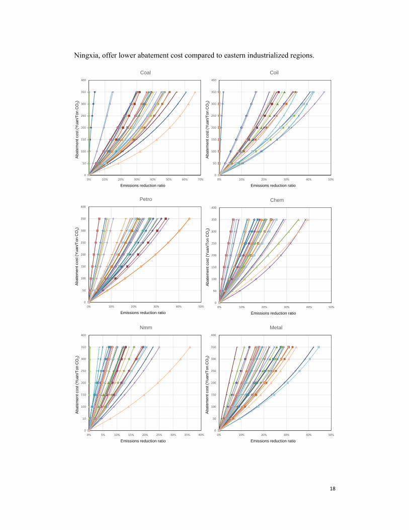
18

Ningxia, offer lower abatement cost compared to eastern industrialized regions.

0

50

100

150

200

250

300

350

400

0% 10% 20% 30% 40% 50% 60% 70%

CoalA

bate

men

t cos

t (Y

uan/

Ton

CO

2)

Emissions reduction ratio

0

50

100

150

200

250

300

350

400

0% 10% 20% 30% 40% 50%

Coil

Aba

tem

ent c

ost (

Yua

n/T

onC

O2)

Emissions reduction ratio

0

50

100

150

200

250

300

350

400

0% 10% 20% 30% 40% 50%

Petro

Aba

tem

ent c

ost (

Yua

n/T

onC

O2)

Emissions reduction ratio

0

50

100

150

200

250

300

350

400

0% 10% 20% 30% 40% 50%

ChemA

bate

men

t cos

t (Y

uan/

Ton

CO

2)

Emissions reduction ratio

0

50

100

150

200

250

300

350

400

0% 5% 10% 15% 20% 25% 30% 35% 40%

Nmm

Aba

tem

ent c

ost (

Yua

n/T

onC

O2)

Emissions reduction ratio

0

50

100

150

200

250

300

350

400

0% 10% 20% 30% 40% 50%

Metal

Aba

tem

ent c

ost (

Yua

n/T

onC

O2)

Emissions reduction ratio

19

Figure 3. Marginal abatement cost curves of energy and energy-intensive sectors in the absence of

ETS

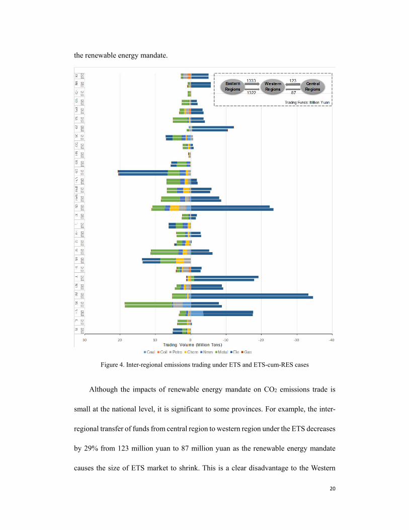
4.2 Carbon market under the policy scenarios

Figure 4 presents trade of CO2 mitigation between the sectors and across the

regions under the ETS (S1) and ETS-cum-RES (S2) scenarios. Under the ETS scenario,

the total trading volume of CO2 mitigation was 173.38 million tons to achieve a target

of reducing 10% CO2 emissions from the base case (i.e., in the absence of these policies).

The equilibrium market price of CO2 price 47.43 yuan/ton (or US$7.1 with exchange

rate of 0.15 US$ for one yuan).

If the separate renewable energy mandate for electricity generation is imposed on

top of the ETS for the same target of CO2 mitigation (i.e., 10% below the base case),

with 50% subsidies for solar, wind, and biomass, the volume of emission trade slightly

decreases, by 1.5%, to170.82 million tons. As a result, the equilibrium CO2 price also

decreases, by 3.5%, to 45.74 yuan/ton. The reduction in trade volume and CO2 price is

caused by the reduction in electricity sectors’ demands for emission allowances due to

0

50

100

150

200

250

300

350

400

0% 10% 20% 30% 40% 50% 60% 70%

Ele

Aba

tem

ent c

ost (

Yua

n/T

onC

O2)

Emissions reduction ratio

0

50

100

150

200

250

300

350

400

0% 10% 20% 30% 40% 50% 60% 70% 80%

Gas

Aba

tem

ent c

ost (

Yua

n/T

onC

O2)

Emissions reduction ratio

Beijing Tianjin Hebei Shanxi InnerMongolia LiaoningJilin Heilongjiang Shanghai Jiangsu Zhejiang AnhuiFujian Jiangxi Shandong Henan Hubei HunanGuangdong Guangxi Hainan Chongqing Sichuan GuizhouYunnan Shaanxi Gansu Qinghai Ningxia Xinjiang

20

the renewable energy mandate.

Figure 4. Inter-regional emissions trading under ETS and ETS-cum-RES cases

Although the impacts of renewable energy mandate on CO2 emissions trade is

small at the national level, it is significant to some provinces. For example, the inter-

regional transfer of funds from central region to western region under the ETS decreases

by 29% from 123 million yuan to 87 million yuan as the renewable energy mandate

causes the size of ETS market to shrink. This is a clear disadvantage to the Western

21

poorer region of adding a separate renewable policy on top of the ETS. The inter-

regional transfer of funds from eastern region to central region, however does not

change much; it gets reduced by less than 1% from 1,333 million yuan to 1,322 million

yuan.

Although the electricity sectors in most regions choose to sell fewer allowances

under the ETS-cum-RES case, the electricity sectors in Hebei, Jilin, Heilongjiang,

Jiangxi, Hubei, and Guizhou will get higher income by selling more allowances

compared to the ETS case. This is because reduction of CO2 in these regions is more

economic despite the shrinkage of the overall carbon market due to higher flexibility of

CO2 reduction from their power sectors. In other words, although the RES policy lowers

the CO2 price and total trading volume, the marginal abatement costs of electricity

sectors in these regions are still less than the CO2 price.

4.3 Economic impacts

Table 4 presents the impacts on key economic variables of the ETS and ETS-cum-

RES policies. Model simulations reveal that ETS would cause less than 0.1% (20 billion

Yuan) reduction in Chinese GDP. However, due to the very large size of Chinese

national GDP, the percentage reduction in GDP appears to be very small. Due to the

expansion of clean infrastructure caused by the ETS policy, there would be a net

increase in total investment by 5 billion Yuan.

22

Table 4. Economic impacts (changes from the base case)

ETS ETS-cum-RES

GDP (million yuan) -20152 (-0.073%) -28105 (-0.101%)

Welfare (million yuan) -10442 -13820

Investment (million yuan) 5037 (0.042%) 4221 (0.035%)

-Eastern regions (million yuan) -183 (-0.003%) -334 (-0.005%)

-Central regions (million yuan) 4301 (0.145%) 3833 (0.129%)

-Western regions (million yuan) 918 (0.038%) 723 (0.030%)

Figure 5a. GDP change in regions under ETS and ETS-cum-RES cases

Figure 5b. Welfare change in regions under ETS and ETS-cum-RES cases

In comparing the economic impacts between the ETS and ETS-cum-RES policy,

we find as expected that the renewable energy mandate plus ETS policy would lead to

-3%

-2%

-1%

0%

1%

2%

3%

BJ TJ HB

SX IM LN JL HLJ

SH JS ZJ AH FJ JX SD HN HB

HN

GD GX

HAN

CQ SC GZ

YN SAXG

SQ

HN

XXJ

ETS ETS-cum-RES

GDP

chan

ge

-15000

-10000

-5000

0

5000

10000

15000BJ TJ H

BSX IM LN JL H

LJSH JS ZJ AH FJ JX SD H

N HB

HN

GD GX

HAN

CQ SC GZ

YN SAXG

SQ

HN

XXJ

ETS ETS-cum-RES

Wel

fare

chan

ge (M

illio

n Yu

an)

23

a larger GDP loss than the ETS alone (though by only about 8 billion, a very small

percentage difference in GDP loss). This is because the RES mandate would have

diverted some of the cheaper reduction that can be achieved through the emission

trading to relatively expensive reduction mandated by the RES policy.

Note that renewable energy sources are supported through subsidy. Necessary

budget to finance the renewable electricity subsidy under the ETS-cum-RES policy is

collected through an additional tax on electricity consumption. The increased electricity

price would reduce the real income of households and thus directly contribute to

reduced household welfare. It also would increase prices of sectoral outputs, especially

of electricity intensive industries and thereby causing reductions in domestic

consumption as well as exports of those goods and ultimately causing the GDP to

decrease. For example, household electricity consumption decreases by 0.58% from the

base case due to the additional RES policy on top of the ETS scheme to meet 10% CO2

emission reduction target in China.

4.4 Impacts on economic structure

4.4.1 Industrial structure

Tables 5 show the changes in sectoral outputs from the base case under ETS and

ETS-cum-RES scenarios. For example, the output of coal industry, the main source of

CO2 emission in China, would drop by 9% under ETS scenario from the base case.

Similarly, sectoral outputs of coal fired electricity generation industry would decrease

by 3%. When the RES policy is added in the presence of the ETS policy, the energy and

energy-intensive industries would experience further output losses. This is because the

24

RES imposes a substitution of fossil fuel based electricity generation with renewable

electricity and would cause reduction of fossil fuel demand for power generation and

thereby fossil fuel supply. Moreover, it also increases electricity prices and causes

outputs of electricity intensive industries to decrease further.

Table 5 Sectoral output change in regions under ETS and ETS-cum-RES cases (%).

Agri Coal Coil Mine Fpap Petro

S1 S2 S1 S2 S1 S2 S1 S2 S1 S2 S1 S2

Total -0.20 -0.21 -8.96 -8.90 -2.98 -3.09 -5.49 -5.48 0.64 0.61 -2.88 -2.92

BJ -0.08 -0.19 -0.50 -0.78 -9.43 -9.18 -0.58 -0.90 0.05 -0.06 -5.89 -6.28

TJ 0.05 0.02 1.99 1.58 -1.83 -1.95 -4.28 -4.39 0.71 0.65 -1.71 -1.82

HB -0.68 -0.75 -17.48 -17.25 -3.24 -3.44 -16.90 -16.75 -1.05 -1.18 -5.96 -6.15

SX -15.36 -14.99 -9.60 -9.14 -5.71 -4.78 -62.52 -61.86 -7.83 -7.53 -0.36 -0.14

IM 1.31 1.34 -5.59 -5.42 1.14 1.02 2.20 2.24 0.99 1.08 -4.85 -4.73

LN -0.20 -0.25 -12.71 -12.59 -1.76 -2.05 -10.16 -10.33 0.48 0.43 0.34 0.03

JL -0.05 -0.08 -9.63 -9.81 -3.33 -3.46 -2.54 -2.87 0.86 0.69 -11.14 -10.81

HLJ -0.59 -0.62 -13.17 -13.60 -3.67 -3.84 -5.43 -5.37 -0.61 -0.65 -3.92 -4.10

SH -0.11 -0.12 0.00 0.00 -1.80 -1.69 0.00 0.00 1.10 1.11 -3.73 -3.66

JS 0.27 0.28 -5.00 -4.94 -3.26 -3.35 -1.18 -1.18 0.52 0.53 -1.33 -1.43

ZJ 0.05 -0.02 -1.33 -1.60 0.00 0.00 -2.49 -2.83 0.41 0.27 -4.21 -3.89

AH -0.35 -0.34 -7.30 -7.17 0.00 0.00 -4.76 -4.55 -0.28 -0.25 -4.03 -4.00

FJ 0.29 0.30 -5.18 -5.22 0.00 0.00 -1.44 -1.34 0.45 0.46 -0.22 -0.29

JX 0.28 0.23 -8.47 -8.72 0.00 0.00 -2.52 -2.87 1.07 0.97 -12.27 -12.34

SD 1.08 1.07 -9.06 -9.13 -4.88 -5.06 -5.35 -5.43 2.72 2.69 -4.61 -4.67

HN -0.43 -0.42 -8.92 -8.85 -2.41 -2.52 -1.17 -1.10 -0.52 -0.49 -3.27 -3.31

HB -0.94 -0.91 2.73 2.25 -26.76 -26.10 -7.89 -7.62 0.12 0.12 -3.81 -3.89

HN -0.70 -0.67 -8.84 -8.75 0.00 0.00 -3.19 -3.09 -0.71 -0.67 -2.16 -2.19

GD 0.42 0.41 0.00 0.00 0.42 0.47 0.12 0.15 1.02 1.00 -0.16 -0.14

GX -0.02 -0.02 -1.57 -1.94 0.00 0.00 -2.93 -2.94 -0.12 -0.11 4.55 4.12

HAN 0.41 0.47 0.00 0.00 0.00 0.00 -1.88 -1.64 0.87 1.02 -3.21 -2.97

CQ -0.14 -0.13 -9.43 -9.21 -30.19 -29.73 -10.21 -9.78 -0.36 -0.32 -11.16 -10.82

SC -0.17 -0.15 -10.26 -10.11 -5.07 -5.03 -5.97 -5.69 0.21 0.25 -21.41 -20.89

GZ -0.35 -0.67 -10.46 -11.32 0.00 0.00 0.89 -0.28 0.78 0.92 -23.46 -22.77

YN -0.09 -0.06 -9.95 -9.75 0.00 0.00 -1.54 -1.42 0.01 0.09 -9.22 -8.94

SAX -0.22 -0.21 -4.35 -4.36 -0.37 -0.42 0.05 0.03 0.16 0.15 -0.85 -0.91

GS 0.64 0.65 -3.65 -3.65 -1.03 -1.06 -1.32 -1.32 0.75 0.78 -0.80 -0.76

QH -0.03 -0.02 -0.55 -0.81 -1.02 -1.11 -3.56 -3.50 -0.37 -0.35 -0.04 -0.17

NX 0.05 -0.02 -8.19 -8.32 -2.88 -3.32 0.00 -0.47 0.12 0.08 -2.82 -3.03

XJ -0.95 -0.98 -18.46 -18.48 -3.90 -3.94 -6.72 -6.59 -0.70 -0.77 -3.02 -3.05

25

Table 5 (continue). Sectoral output change in regions under ETS and ETS-cum-RES cases (%).

Chem Nmm Metal Omf Ele Gas

S1 S2 S1 S2 S1 S2 S1 S2 S1 S2 S1 S2

Total -1.17 -1.23 -1.98 -1.98 -4.84 -4.81 -0.77 -0.77 -3.02 -3.31 -0.87 -1.19

BJ -1.21 -1.39 -0.92 -1.01 -1.39 -1.46 0.47 0.39 -3.22 -4.28 -0.95 -1.26

TJ -0.09 -0.11 -0.31 -0.26 -2.33 -2.23 -0.04 -0.01 -1.77 -1.61 0.44 0.11

HB -1.30 -1.54 -3.64 -3.67 -10.04 -9.96 -4.33 -4.38 -6.56 -7.02 -4.29 -4.71

SX -36.28 -35.36 -9.14 -8.92 -25.32 -24.96 -12.19 -11.82 0.92 1.13 0.62 0.71

IM 5.16 4.91 2.12 2.12 -1.65 -1.57 0.12 0.09 -1.51 -1.47 0.17 0.15

LN -0.40 -0.63 -1.55 -1.70 -12.27 -12.17 -1.43 -1.48 -6.12 -6.70 -8.50 -9.15

JL -1.49 -1.92 -6.55 -6.59 -18.40 -18.11 -0.24 -0.27 -7.11 -9.10 -3.89 -5.25

HLJ -2.08 -2.06 -2.81 -2.82 -5.36 -5.24 -1.04 -1.06 -5.31 -5.98 -6.38 -6.84

SH -1.02 -0.99 0.14 0.18 -2.47 -2.34 0.25 0.25 -1.23 -1.01 -0.13 -0.30

JS -0.08 -0.06 -0.77 -0.73 -0.55 -0.51 -0.54 -0.50 -1.61 -1.56 -0.14 -0.26

ZJ -0.24 -0.53 -0.85 -0.95 1.68 1.30 -1.84 -1.95 -4.10 -4.86 0.11 -0.96

AH -2.11 -2.03 -2.68 -2.60 -3.08 -2.91 -2.04 -1.93 -2.67 -2.68 -1.19 -1.32

FJ -0.22 -0.19 -1.52 -1.46 -0.81 -0.74 0.22 0.24 -1.37 -1.47 0.70 0.46

JX 1.44 1.27 -2.92 -2.92 -5.59 -5.63 -0.77 -0.83 -5.25 -6.04 -0.02 -0.42

SD -1.63 -1.73 -2.30 -2.40 -8.61 -8.52 -2.22 -2.19 -2.85 -2.85 -1.34 -1.69

HN -0.42 -0.40 -0.86 -0.81 -0.86 -0.81 -0.21 -0.21 -2.92 -3.03 -2.15 -2.28

HB -7.25 -7.01 -4.75 -4.57 -10.21 -9.85 -0.87 -0.84 -5.03 -5.58 0.34 0.20

HN -2.59 -2.53 -4.60 -4.46 -2.57 -2.49 -1.53 -1.49 -2.49 -2.49 -0.58 -0.71

GD 0.74 0.73 -0.29 -0.28 0.73 0.72 0.40 0.40 -1.08 -1.09 0.59 0.41

GX 0.10 0.05 -2.96 -2.93 -2.21 -2.22 -0.77 -0.78 -3.29 -3.67 -0.53 -1.28

HAN -16.64 -15.81 -0.93 -0.81 -11.26 -10.57 1.25 1.36 2.21 2.48 0.01 0.15

CQ -8.17 -7.84 -5.69 -5.42 -6.86 -6.62 -3.36 -3.25 -2.83 -2.60 0.42 0.19

SC -0.60 -0.57 -3.09 -2.98 -8.34 -8.02 -2.98 -2.87 -2.52 -2.57 -0.83 -0.86

GZ 2.85 1.96 -1.68 -2.30 -9.49 -12.94 -0.29 -0.71 -8.02 -10.64 -18.20 -23.42

YN 0.01 0.03 -1.54 -1.47 -1.28 -1.17 -0.33 -0.26 -2.01 -2.04 -1.27 -1.25

SAX -3.41 -3.29 -0.04 -0.06 0.83 0.78 -0.54 -0.57 -1.87 -1.86 -0.09 -0.27

GS 0.10 0.09 -2.07 -2.03 -1.82 -1.79 -0.56 -0.56 -1.37 -1.32 0.55 0.23

QH -3.25 -3.27 -0.17 -0.16 -3.40 -3.39 0.46 0.51 -2.11 -2.26 -0.39 -0.49

NX -1.20 -1.46 -2.78 -2.88 0.56 -0.29 0.44 0.11 -4.09 -4.83 -0.53 -1.10

XJ -12.36 -12.30 -3.11 -3.10 -6.00 -5.91 -3.04 -3.09 -6.28 -6.56 -3.17 -3.36

26

Table 5 (continue). Sectoral output change in regions under ETS and ETS-cum-RES cases (%).

Cons Trans Wsale Esta Ots

S1 S2 S1 S2 S1 S2 S1 S2 S1 S2

Total -0.16 -0.16 -1.43 -1.41 -0.75 -0.74 -0.99 -0.96 -0.50 -0.50

BJ -0.06 -0.07 -0.32 -0.35 0.06 -0.01 -0.04 -0.07 0.10 0.04

TJ -0.39 -0.40 -1.17 -1.10 -0.44 -0.40 -0.93 -0.86 -0.13 -0.12

HB -0.23 -0.24 -3.77 -3.83 -3.02 -3.06 -3.91 -3.96 -2.72 -2.79

SX -2.28 -2.23 -17.39 -16.82 -10.88 -10.52 -16.91 -16.47 -3.08 -2.90

IM 0.04 0.04 -1.31 -1.18 0.08 0.08 -1.05 -0.96 0.15 0.18

LN -0.10 -0.10 -2.21 -2.24 -1.75 -1.80 -2.47 -2.47 -1.54 -1.58

JL -0.19 -0.19 -0.93 -1.02 -0.50 -0.62 -1.22 -1.32 -0.79 -0.91

HLJ -0.16 -0.16 -2.66 -2.67 -1.76 -1.79 -2.00 -2.02 -1.38 -1.45

SH -0.06 -0.05 -0.52 -0.46 -0.23 -0.19 -0.27 -0.24 0.01 0.03

JS -0.01 -0.01 -0.40 -0.35 -0.14 -0.11 -0.43 -0.37 0.07 0.10

ZJ -0.04 -0.04 -0.69 -0.76 -0.27 -0.32 -0.35 -0.44 -0.32 -0.39

AH -0.20 -0.19 -1.56 -1.47 -0.92 -0.86 -0.91 -0.84 -0.80 -0.75

FJ 0.01 0.01 -0.16 -0.12 0.13 0.16 -0.41 -0.34 0.13 0.16

JX -0.08 -0.08 -2.59 -2.61 -1.03 -1.12 -0.96 -1.01 -0.59 -0.64

SD -0.05 -0.05 -0.31 -0.24 1.06 1.07 -0.85 -0.82 0.15 0.14

HN 0.01 0.01 -1.05 -1.01 -1.16 -1.11 -1.08 -1.01 -0.70 -0.68

HB -0.44 -0.43 -3.19 -3.09 -2.21 -2.14 -3.74 -3.63 -1.97 -1.91

HN -0.66 -0.64 -1.56 -1.50 -1.33 -1.28 -1.48 -1.40 -0.99 -0.94

GD 0.07 0.05 0.49 0.51 0.58 0.60 0.49 0.50 0.46 0.47

GX -0.24 -0.24 -0.67 -0.65 -0.78 -0.75 -0.70 -0.66 -0.30 -0.30

HAN -0.02 -0.02 -1.21 -0.99 0.41 0.56 -0.98 -0.81 0.20 0.28

CQ -0.27 -0.27 -1.77 -1.69 -1.99 -1.92 -1.68 -1.59 -0.60 -0.56

SC -0.08 -0.07 -3.33 -3.21 -2.63 -2.52 -2.53 -2.42 -1.31 -1.25

GZ 0.01 -0.08 -3.32 -3.98 -2.09 -2.69 -3.78 -4.15 -0.83 -1.20

YN -0.06 -0.06 -1.62 -1.51 -1.33 -1.22 -1.73 -1.59 -0.07 -0.02

SAX 0.38 0.39 -0.69 -0.68 -0.30 -0.31 -0.18 -0.17 -0.54 -0.55

GS -0.61 -0.61 1.92 1.93 2.04 2.11 0.03 0.07 0.25 0.26

QH -0.09 -0.09 -0.65 -0.65 -0.37 -0.37 -1.20 -1.19 -0.11 -0.12

NX -0.02 -0.03 -1.60 -1.72 -1.18 -1.29 -1.80 -1.78 -0.05 -0.18

XJ -0.13 -0.13 -2.83 -2.80 -1.51 -1.53 -2.53 -2.48 -1.99 -1.99

Note:

1. S1 and S2 denote ETS and ETS-cum-RES cases, respectively.

2. The value 0 in the table indicates zero output of that sector in the base case.

The results show that the outputs in transport, wholesale, real estate, and other

services sectors under ETS-cum-RES case are more than the ETS case. This is because

the RES policy would create more demand for goods and services to be produced from

27

these sectors to support expansion of renewable energy industries in China.

4.4.2 Power generation mix

Table 6 presents the power generation mix under the various scenarios and

percentage change in outputs of each power generation technology. Note that the drops

in electricity outputs of from fossil fuel based technologies are higher under the ETS-

cum-RES scenario are higher as compared to that in ETS scenario. This is because the

RES policy causes substitution of fossil fuel based power generation with the renewable

energy based electricity.

Table 6. Generation mix (%) under different scenarios along with percentage change in electricity

outputs of different generation technologies S0 ETS ETS-cum-RES

Proportion Change Proportion Change Proportion

Coa 84.870 -3.024 84.866 -3.591 84.335

Ngs 1.672 -2.938 1.673 -3.487 1.663

Pet 3.404 -3.615 3.383 -3.955 3.370

Nuc 1.648 -2.790 1.651 -3.413 1.640

Hyd 7.703 -2.790 7.721 0.045 7.943

Win 0.536 -2.790 0.537 44.559 0.799

Sol 0.127 -2.790 0.127 44.559 0.189

Oth 0.040 -2.790 0.041 44.559 0.060

Interestingly, electricity generation from renewable as well as fossil sources is

decreasing under the ETS scenario. The reason is that the nesting structure used to

model electricity generation technologies (Figure 1) does not allow different

substitution possibility between the aggregate electricity generation from fossil fuels

and aggregate electricity generation from renewable energy sources. Since the share of

non-fossil share of total electricity generation is relatively small (< 10%) in China, this

28

rigid nesting structure adopted in the model used for this study would not impact the

result much for a small carbon price. However, the model structure must be changed to

allow the substitution effect to work if carbon pricing level is high.

4.4.3 Impacts on residential consumption of goods and services

Table 7 presents the impacts of ETS and ETS-cum-RES scenarios on household

consumption of goods and services. From the table, three observations can be made.

First, under the both schemes, household consumption of fossil fuels and energy

intensive products (non-metallic minerals, metals, chemicals) would drop by higher

proportions than other goods and services. Second, the drops in household consumption

of goods and services would be higher under ETS-cum-RES scenario than that of ETS

scenario. The difference in drops of electricity consumption between the ETS and ETS-

cum-RES scenario is noticeable as the adoption of RES policy increases the price for

electricity consumption, and thus leads to significant decrease of electricity

consumption, comparing with the ETS case. Third, the drops of household consumption

of good and services are much higher in some provinces (e.g., Hebei, Liaoning,

Heilongjiang, Guizhou, Hainan, Xinjiang) than in other provinces. This is because

households in these provinces consume proportionally higher amounts of energy and

energy intensive goods and services.

29

Table 7. Change in household consumption from the base case (%).

Agriculture Coal Crude oil Mining Food, paper Petroleum

S1 S2 S1 S2 S1 S2 S1 S2 S1 S2 S1 S2

Total -0.05 -0.07 -0.80 -0.80 -0.47 -0.49 -0.55 -0.54 -0.12 -0.14 -0.54 -0.54

BJ 0.18 0.13 -0.09 -0.12 0.00 0.00 0.00 0.00 0.17 0.12 -0.44 -0.47

TJ 0.15 0.15 -0.29 -0.26 0.03 0.05 0.34 0.32 0.11 0.11 -0.48 -0.46

HB -2.35 -2.40 -3.40 -3.42 -2.67 -2.72 -1.84 -1.95 -2.50 -2.57 -3.18 -3.21

SX 1.81 1.89 0.27 0.39 0.00 0.00 0.00 0.00 1.74 1.82 0.08 0.23

IM 0.39 0.42 0.83 0.87 0.69 0.73 0.00 0.00 0.57 0.60 -0.21 -0.15

LN -1.00 -1.07 -1.41 -1.45 -1.35 -1.41 0.00 0.00 -1.07 -1.15 -1.53 -1.58

JL -0.40 -0.52 -0.62 -0.69 -0.50 -0.62 0.00 0.00 -0.52 -0.65 -1.17 -1.26

HLJ -1.31 -1.38 0.14 0.13 -1.50 -1.56 0.00 0.00 -1.32 -1.40 -2.32 -2.35

SH 0.26 0.28 -0.14 -0.10 0.00 0.00 0.00 0.00 0.14 0.16 -0.61 -0.56

JS 0.40 0.42 0.03 0.07 0.00 0.00 0.00 0.00 0.50 0.52 -0.02 0.02

ZJ 0.19 0.09 -0.14 -0.23 0.00 0.00 0.00 0.00 0.18 0.05 -0.29 -0.39

AH -0.29 -0.25 -0.76 -0.70 0.00 0.00 0.00 0.00 -0.37 -0.34 -1.11 -1.04

FJ 0.36 0.38 0.63 0.67 0.33 0.36 0.00 0.00 0.48 0.50 -0.10 -0.06

JX -0.10 -0.15 -0.31 -0.35 -0.26 -0.33 0.00 0.00 -0.13 -0.21 -0.95 -0.99

SD 0.00 -0.02 -0.55 -0.55 0.00 0.00 0.20 0.13 0.07 0.04 -0.38 -0.39

HN -0.18 -0.16 -1.45 -1.40 -0.57 -0.55 -0.56 -0.55 -0.21 -0.20 -1.25 -1.19

HB -0.77 -0.74 -1.25 -1.20 0.00 0.00 -0.68 -0.68 -0.77 -0.75 -1.68 -1.62

HN -0.50 -0.46 -1.69 -1.59 -1.04 -0.98 0.00 0.00 -0.74 -0.70 -1.52 -1.44

GD 0.86 0.86 0.47 0.48 0.78 0.79 0.90 0.88 0.85 0.84 0.52 0.53

GX -0.05 -0.04 -0.36 -0.33 0.00 0.00 0.00 0.00 -0.06 -0.06 -0.60 -0.57

HAN -0.21 -0.10 -0.40 -0.27 0.00 0.00 0.00 0.00 -0.17 -0.05 -0.64 -0.51

CQ -0.24 -0.21 0.00 0.00 -0.71 -0.66 0.00 0.00 -0.35 -0.32 -1.15 -1.09

SC -0.42 -0.39 -1.51 -1.41 -0.87 -0.81 0.00 0.00 -0.54 -0.50 -1.66 -1.57

GZ -0.84 -1.40 -0.62 -1.10 -1.16 -1.90 0.00 0.00 -0.94 -1.64 -1.85 -2.47

YN 0.20 0.24 -0.53 -0.46 0.00 0.00 0.00 0.00 0.15 0.20 -1.12 -1.03

SAX -0.03 -0.04 0.08 0.08 0.00 0.00 -0.12 -0.15 -0.10 -0.11 -0.69 -0.67

GS 0.78 0.79 1.07 1.10 0.00 0.00 1.06 1.05 0.88 0.88 0.50 0.52

QH 0.04 0.04 -0.32 -0.27 -0.59 -0.55 0.00 0.00 0.06 0.06 -0.06 -0.01

NX 0.40 0.24 0.21 0.13 0.23 0.05 0.00 0.00 0.50 0.31 -0.57 -0.71

XJ -1.06 -1.08 0.32 0.32 -2.16 -2.15 0.00 0.00 -1.44 -1.48 -2.78 -2.75

Note:

1. S1 and S2 denote ETS and ETS-cum-RES cases, respectively.

2. The value 0 in the table indicates there is no household consumption of commodities in the base

case.

30

Table 7b. Household consumption change in regions under ETS and ETS-cum-RES cases (%).

Chemicals Non metals Metal Other MF Electricity Gas

S1 S2 S1 S2 S1 S2 S1 S2 S1 S2 S1 S2

Total -0.42 -0.47 -0.86 -0.87 -1.09 -1.09 -0.26 -0.28 -0.05 -0.58 -0.39 -0.39

BJ -0.11 -0.18 -0.25 -0.31 -0.75 -0.79 -0.06 -0.11 0.37 -0.67 0.18 0.11

TJ -0.12 -0.12 -0.27 -0.28 -0.87 -0.85 -0.12 -0.11 0.45 0.08 -0.06 -0.04

HB -2.84 -2.91 -2.69 -2.76 -3.85 -3.89 -2.97 -3.03 -2.76 -3.39 -2.46 -2.50

SX 0.80 0.91 0.64 0.74 -1.02 -0.86 1.21 1.30 1.46 1.47 1.31 1.40

IM 0.37 0.39 0.01 0.03 -0.36 -0.32 0.34 0.36 3.58 3.24 0.33 0.38

LN -1.37 -1.45 -1.68 -1.77 -2.23 -2.28 -1.40 -1.47 -1.17 -2.25 -1.33 -1.39

JL -0.77 -0.91 -1.28 -1.41 -1.58 -1.69 -0.79 -0.91 -0.01 -0.73 -0.81 -0.92

HLJ -1.70 -1.79 -2.38 -2.46 -2.64 -2.70 -1.68 -1.76 -1.05 -1.82 -2.83 -2.93

SH -0.12 -0.10 -0.12 -0.11 -0.40 -0.36 -0.02 0.01 0.50 0.22 -0.06 -0.03

JS 0.30 0.31 0.02 0.03 -0.31 -0.28 0.25 0.28 0.79 0.49 0.17 0.20

ZJ -0.05 -0.18 -0.39 -0.52 -0.81 -0.91 -0.13 -0.25 -0.33 -1.08 0.01 -0.11

AH -0.71 -0.67 -1.29 -1.25 -1.51 -1.45 -0.73 -0.68 -1.08 -1.33 -0.56 -0.52

FJ 0.21 0.23 -0.26 -0.24 -0.51 -0.47 0.24 0.26 1.10 0.79 0.25 0.25

JX -0.24 -0.32 -0.72 -0.80 -1.13 -1.20 -0.30 -0.37 -0.22 -0.88 -0.25 -0.34

SD -0.06 -0.09 -0.10 -0.12 -0.64 -0.65 -0.06 -0.09 0.97 0.55 -0.09 -0.12

HN -0.50 -0.50 -0.71 -0.70 -1.32 -1.29 -0.64 -0.62 -0.74 -1.14 -1.28 -1.26

HB -1.33 -1.30 -1.94 -1.89 -1.74 -1.70 -1.01 -0.99 -0.22 -0.74 -0.91 -0.88

HN -1.28 -1.24 -2.11 -2.05 -1.89 -1.82 -1.16 -1.11 -0.57 -0.86 -0.97 -0.95

GD 0.69 0.68 0.36 0.35 0.24 0.24 0.67 0.67 0.88 0.59 0.67 0.68

GX -0.26 -0.27 -1.66 -1.66 -1.24 -1.24 -0.36 -0.36 -0.10 -0.69 -0.25 -0.29

HAN -0.39 -0.28 -0.59 -0.47 -0.76 -0.64 -0.37 -0.25 -0.27 -0.14 -0.37 -0.26

CQ -0.75 -0.72 -1.08 -1.05 -1.27 -1.23 -0.66 -0.63 0.08 -0.30 -0.46 -0.42

SC -0.75 -0.72 -1.36 -1.30 -1.60 -1.54 -0.86 -0.81 -1.16 -1.44 -0.72 -0.68

GZ -1.16 -1.89 -1.58 -2.25 -1.96 -2.68 -1.23 -1.92 0.65 -1.44 0.49 0.35

YN -0.08 -0.04 -0.94 -0.89 -1.01 -0.94 -0.16 -0.12 2.83 2.40 -0.36 -0.30

SAX -0.42 -0.44 -0.53 -0.55 -1.04 -1.04 -0.40 -0.41 0.17 -0.19 -0.26 -0.25

GS 0.67 0.67 0.33 0.33 0.08 0.09 0.71 0.71 1.69 1.38 0.93 0.98

QH -1.46 -1.47 -0.21 -0.20 -1.26 -1.33 -0.19 -0.18 1.40 0.91 -0.21 -0.19

NX 0.12 -0.10 -0.53 -0.72 -0.30 -0.54 0.23 0.03 2.77 1.79 0.36 0.22

XJ -1.92 -1.95 -2.54 -2.57 -2.81 -2.81 -1.87 -1.89 -4.45 -5.12 -1.66 -1.70

31

Table 7c. Household consumption change in regions under ETS and ETS-cum-RES cases (%).

Construction Transport Wholesale Real Estate Others

S1 S2 S1 S2 S1 S2 S1 S2 S1 S2

Total -0.52 -0.55 -0.03 -0.05 0.08 0.05 0.05 0.04 -0.11 -0.13

BJ -0.21 -0.26 0.14 0.08 0.25 0.20 0.19 0.15 0.08 0.03

TJ -0.25 -0.24 0.13 0.13 0.26 0.27 0.28 0.29 0.14 0.14

HB -2.93 -3.00 -2.31 -2.39 -2.23 -2.29 -2.25 -2.31 -2.25 -2.33

SX 0.00 0.00 2.00 2.08 2.01 2.09 2.04 2.12 1.63 1.72

IM 0.27 0.30 0.66 0.69 0.75 0.77 0.79 0.82 0.64 0.66

LN -1.49 -1.57 -0.99 -1.06 -0.78 -0.85 -0.71 -0.78 -0.82 -0.89

JL -0.90 -1.03 -0.52 -0.65 -0.43 -0.56 -0.41 -0.53 -0.39 -0.52

HLJ -1.85 -1.93 -1.32 -1.40 -1.30 -1.39 -1.22 -1.30 -1.22 -1.31

SH 0.00 0.00 0.17 0.19 0.27 0.30 0.24 0.28 0.12 0.14

JS 0.21 0.23 0.46 0.49 0.55 0.58 0.56 0.59 0.47 0.49

ZJ -0.37 -0.49 0.15 0.04 0.24 0.13 0.24 0.14 0.17 0.06

AH -0.80 -0.76 -0.41 -0.37 -0.30 -0.26 -0.36 -0.31 -0.35 -0.32

FJ 0.19 0.21 0.48 0.50 0.54 0.57 0.53 0.56 0.48 0.49

JX -0.62 -0.71 0.07 -0.02 0.04 -0.07 0.11 0.04 0.13 0.05

SD -0.15 -0.17 0.06 0.04 0.04 0.02 0.30 0.29 0.09 0.06

HN -0.62 -0.61 -0.26 -0.24 -0.13 -0.11 -0.28 -0.26 -0.19 -0.19

HB -1.32 -1.28 -0.49 -0.48 -0.41 -0.40 -0.21 -0.20 -0.42 -0.41

HN -1.27 -1.22 -0.81 -0.76 -0.60 -0.56 -0.73 -0.68 -0.66 -0.62

GD 0.65 0.62 0.85 0.86 0.91 0.91 0.88 0.90 0.78 0.78

GX -0.62 -0.62 0.02 0.02 0.04 0.04 0.02 0.03 0.01 0.01

HAN -0.32 -0.19 -0.22 -0.10 -0.15 -0.02 -0.06 0.06 -0.24 -0.12

CQ -0.83 -0.80 -0.31 -0.29 -0.25 -0.22 -0.20 -0.18 -0.35 -0.32

SC -1.03 -0.98 -0.50 -0.45 -0.42 -0.38 -0.31 -0.27 -0.41 -0.37

GZ -1.25 -1.99 -0.68 -1.36 -0.71 -1.40 -0.65 -1.30 -0.71 -1.37

YN -0.36 -0.31 0.06 0.11 0.24 0.29 0.27 0.31 0.13 0.17

SAX -0.46 -0.47 -0.11 -0.12 0.00 -0.01 0.14 0.13 0.03 0.02

GS 0.68 0.69 0.75 0.76 0.84 0.85 0.96 0.97 0.90 0.90

QH -0.26 -0.26 0.11 0.12 0.13 0.13 0.17 0.17 0.09 0.08

NX 0.11 -0.09 0.57 0.38 0.64 0.46 0.64 0.46 0.53 0.35

XJ -1.58 -1.61 -1.44 -1.47 -1.39 -1.41 -1.25 -1.27 -1.28 -1.31

4.4.4 Export and import

Figure 6 presents the impacts on export and import of total goods and services

under ETS and ETS-cum-RES scenarios. Both ETS and ETS-cum-RES scenarios

would cause exports of fossil fuels and energy intensive goods to decrease and exports

32

of low emission intensive goods and services to increase. The magnitudes of changes

in exports are lower under the ETS-cum-RES policy as compared to ETS policy.

The total import would also drop in China under ETS and ETS-cum-RES cases,

respectively. The difference of import impacts between the ETS and ETS-cum-RES

scenarios is not significant. As expected imports of fossil fuels would decrease under

both scenarios. Note that although China is rich in coal resources, it is a net importer of

coal due to much higher demand compared to domestic supply. While the reductions of

imports of most commodities are less than 2%, the reductions of import of coal and

mining products are more than 6%.

Figure 6. Changes of sectoral export and import under ETS and ETS-cum-RES cases

5. Conclusion

The emissions trading scheme and renewable energy mandates are two key

elements in the climate change mitigation policy package that the government is

implementing in China to achieve its nationally determined commitments under the

Paris Agreement. In order to understand the interactions between these instruments, this

-12%

-10%

-8%

-6%

-4%

-2%

0%

2%

4%

6%

Ag

ri

Co

al

Co

il

Min

e

Fp

ap

Pe

tro

Ch

em

Nm

m

Me

tal

Om

f

Ele

Ga

s

Co

ns

Tra

ns

Ws

ale

Es

ta

Ots

S1_Export S2_Export S1_Import S2_Import

Exp

ort

/ Im

port

Cha

nge

33

study compares economy-wide impacts of ETS with and without a separate RES. These

impacts are measured using a multi-regional computable general equilibrium model of

China. Understanding these interactions would be helpful in designing the national

emission trading scheme that China is going to introduce in 2017.

Our analysis shows that to achieve 10% reduction of CO2 emissions in China from

the base case, a national emission trading scheme would cause a slight loss of GDP and

welfare. If a separate renewable electricity mandate is introduced on top of the ETS to

achieve the same level of CO2 mitigation, it would cause greater GDP and welfare

losses. This would happen because an ETS allows the market to find and implement the

cheapest GHG mitigation options. When a renewable energy mandate is imposed, it

diverts resources into implementing the renewable energy technologies versus other

GHG mitigation options which are cheaper than the renewable energy technologies.

The additional RES policy mandate would decrease the demand for emission

allowances in trading sectors, thereby causing the size of the carbon market to shrink

and the equilibrium carbon price to drop. This would lower the inter-provincial as well

as inter-sectoral transfer of funds associated with emission trading. Our study shows

that the inter-regional transfer of funds from the central region to the western region

under the ETS decreases by 29% as the renewable energy mandate causes the size of

the ETS market to shrink.

Despite the political appetite for mixing various GHG mitigation options to

mitigate climate change, this study quantitatively demonstrates that relying on carbon

pricing would be more efficient to achieve a given target of climate change mitigation.

34

While other policies such as renewable energy standards or energy efficiency mandates

are promoted as well as GHG mitigation, their imposition is not necessary to achieve a

climate change mitigation target if an emission trading scheme is already in place to

meet the same objective.

It is important to note that a renewable energy policy together with an ETS would

reduce more fossil fuels than the ETS policy alone and therefore help reduce more local

air pollution than the latter. Considering the importance of local air pollution reduction

in China, if the benefits from local air pollution are quantified and accounted for in the

model, one could argue that the ETS cum RES policy might be more economic than the

ETS policy alone. However, quantification of local air pollution reduction benefits in

each of the 30 provinces in our model is itself huge task and beyond the scope of this

study. 10 Moreover, the model needs substantial modification because its current

welfare measure does not account for environmental benefits coming from CO2

mitigation and local air pollution mitigation. These could be considerations for future

studies.

It is also important to note that in practice emission trading schemes do not

necessarily capture all potential emission sources. In such cases additional policy

instruments can be helpful. Moreover, a separate renewable energy target may be

needed if government, for whatever reasons, would like to see more deployment of

renewable energy in addition to GHG mitigation.

10 It is further complicated considering the trans-boundary nature of local air pollutants.

35

References

Böhringer, C., Behrens, M., 2015. Interactions of emission caps and renewable electricity support

schemes. Journal of Regulatory Economics 48(1), 74-96.

Böhringer, C., Löschel, A., Moslener, U., et al., 2009. EU climate policy up to 2020: An economic

impact assessment. Energy Economics 31, S295-S305.

Cao, J., Ho, M. and Timilsina, G.R. (2016). Impacts of Carbon Pricing in Reducing the Carbon

Intensity of China’s GDP, World Bank Policy Research Working Paper, WPS 7735. World

Bank, Washington, DC.

Couture, T., Gagnon, Y., 2010. Analysis of feed-in tariff remuneration models: implications for

renewable energy investment. Energy Policy 38(2), 955-965.

Fan Y., Wu J., Xia Y., et al., 2016. How will a nationwide carbon market affect regional economies

and efficiency of CO2 emission reduction in China? China Economic Review 38, 151-166.

Fankhauser, S., Hepburn, C., Park, J., 2010. Combining multiple climate policy instruments: how

not to do it. Climate Change Economics 1(3), 209-225.

He, Y.X., Pang, Y.X., Zhang, J.X., et al., 2015. Feed-in tariff mechanisms for large-scale wind power

in China. Renewable and Sustainable Energy Reviews 51, 9-17.

Hübler, M., Voigt, S., Löschel, A., 2014. Designing an emissions trading scheme for China—An up-

to-date climate policy assessment. Energy Policy 75, 57-72.

Landis, F. and G.R. Timilsina (2015). The Economics of Policy Instruments to Stimulate Wind

Power in Brazil, World Bank Policy Research Working Paper, WPS 7376, World Bank.

Washington, DC.

Langniß, O., Diekmann, J., Lehr, U., 2004. Advanced mechanisms for the promotion of renewable

36

energy—Models for the future evolution of the German Renewable Energy Act. Energy Policy

37(4), 1289-1297.

Lesser, J.A., Su, X.J., 2008. Design of an economically efficient feed-in tariff structure for

renewable energy development. Energy Policy 36, 981-990.

Lin, W.B., Gu, A., Wang, X., et al., 2016. Aligning emissions trading and feed-in tariffs in China.

Climate Policy 16(4), 434-455.

Morris, J.F., 2009. Combining a renewable portfolio standards with a cap-and-trade policy: a general

equilibrium analysis. Massachusetts Institute of Technology.

National Development and Reform Commission (NDRC), 2015. China's Intended Nationally

Determined Contribution: Enhanced Actions on Climate Change. Available at:

http://www.sdpc.gov.cn/xwzx/xwfb/201506/t20150630_710204.html.

Newell, R. (2015). The Role of Energy Technology Policy alongside Carbon Pricing. Parry, I.W.

(ed.) Implementing a US Carbon Tax: Challenges and Debates. Routledge.

Nordhaus, W., 2011.Designing a friendly space for technological change to slow global warming.

Energy Economics 33, 665-673.

Ouyang, X.L., Lin, B.Q., 2014. Levelized cost of electricity (LCOE) of renewable energies and

required subsidies in China. Energy Policy 70, 64-73.

Schallenberg-Rodriguez, J., Haas, R., 2012.Fixed feed-in tariff versus premium: a review of the

current Spanish system. Renewable and Sustainable Energy Reviews 16(1), 293-305.

Timilsina, G.R. and F. Landis (2014). Economics of Transiting to Renewable Energy in Morocco:

A General Equilibrium Analysis, World Bank Policy Research Working Paper, WPS 6940,

World Bank. Washington, DC.

37

Tsao, C.-C., Campbell, J.E., Chen, Y., 2011.When renewable portfolio standards meet cap-and-trade

regulations in the electricity sector: Market interactions, profits implications, and policy

redundancy. Energy Policy 39(7), 3966-3974.

Van den Bergh, K., Delarue, E., D’haeseleer, W, 2013. Impact of renewables deployment on the

CO2 price and the CO2 emissions in the European electricity sector. Energy Policy 63, 1021-

1031.

Weigt, H., Ellerman, A.D., Delarue, E., 2013. CO2 abatement from renewables in the German

electricity sector: does a CO2 price help? Energy Economics 40, 149-158.

Wu J., Fan Y., Xia Y., 2016. The economic effects of initial quota allocations on carbon emissions

trading in China. The Energy Journal 37(SI1), 129-151.

Zhang, S., Bauer, N., 2013.Utilization of the non-fossil fuel target and its implications in China.

Climate Policy 13, 328-344.