DPRIETI Discussion Paper Series 18-E-010

Uncertainty, Imperfect Information,and Learning in the International Market

CHEN ChengUniversity of Hong Kong

SENGA TatsuroRIETI

SUN ChangUniversity of Hong Kong

ZHANG HongyongRIETI

The Research Institute of Economy, Trade and Industryhttp://www.rieti.go.jp/en/

RIETI Discussion Paper Series 18-E-010 March 2018

Uncertainty, Imperfect Information, and Learning in the International Market*

CHEN Cheng† SENGA Tatsuro‡ SUN Chang§ ZHANG Hongyong**

Abstract

This paper uses a unique dataset of Japanese multinational affiliates, which contains information on sales forecasts, to detect information imperfection and learning in the international market. We document three stylized facts concerning affiliates' forecasts. First, forecast errors (FEs) of sales decline with the affiliate's age. Second, if the parent firm has previous export experience to the region where its affiliate is set up, the entering affiliate starts with a smaller absolute value of FEs. Third, FEs of sales are positively correlated over time and this positive correlation becomes stronger when the affiliates are located further away from Japan. In total, we view these facts as direct evidence for the existence of imperfect information and learning in the international market. We then build up and quantify a dynamic industry equilibrium model of trade and foreign direct investment (FDI), which features information rigidity and learning, in order to explain the documented facts. Counterfactual analysis shows that the variance of time-invariant demand draws and that of transitory shocks have qualitatively different and quantitatively important implications for dynamic patterns of trade/multinational production, dynamic selection, and aggregate productivity. Keywords: Imperfect information and learning, Uncertainty and firm expectations, Time-invariant and transitory shocks, Multinational firms, Firm dynamics JEL classification: F1; F2; D83; D84; E23

RIETI Discussion Papers Series aims at widely disseminating research results in the form of professional papers, thereby stimulating lively discussion. The views expressed in the papers are solely those of the author(s), and neither represent those of the organization to which the author(s) belong(s) nor the Research Institute of Economy, Trade and Industry.

* This research was conducted as a part of the research project “Studies on Firm Management and Internationalization under the Growing Fluidity of the Japanese Economy” at the Research Institute of Economy, Trade and Industry (RIETI). We are grateful to the Ministry of Economy, Trade and Industry (METI) for providing the micro-data of the Basic Survey of Japanese Business Structure and Activities and the Basic Survey on Overseas Business Activities, and grateful to RIETI for providing the Kikatsu-Kaiji converter. We would like to thank Masayuki Morikawa, Makoto Yano, Keisuke Kondo, Shang-Jin Wei, and seminar participants at RIETI for helpful comments. Financial support from HKGRF, RIETI, KAKENHI (17H02531) and the International Economics Section at Princeton University is greatly appreciated. † University of Hong Kong. Email: ccfour@hku.hk. ‡ Queen Mary University of London, ESCoE, and RIETI. Email: t.senga@qmul.ac.uk. § University of Hong Kong. Email: sunc@hku.hk. ** RIETI. Email: zhang-hong-yong@rieti.go.jp

1 Introduction

When firms enter new markets, they face considerable uncertainty and information imperfection.

Other than macroeconomic fluctuations induced by business cycles or government policies, firms

also face uncertainty and information imperfection at the microeconomic level. This is especially

true for firms that enter foreign markets. For instance, exporters or multinational affiliates may

not know how popular their products would be in the foreign market before entry. Naturally, such

an information problem can be resolved by gradually discovering and learning the popularity of

their products after entry. Moreover, for firms that plan to do foreign direct investment (FDI)

and multinational production (MP), they may use the strategy of sequential entry (i.e., using

exporting as an intermediate stage before FDI) to acquire information about their demand.

In this paper, we utilize a unique dataset of Japanese multinational enterprises (MNEs) which

contains information on sales forecasts at the affiliate level to detect information imperfection

and learning in the international market.

Two strands of literature have started to investigate how uncertainty and information im-

perfection affect firm dynamics and trade patterns. The empirical macroeconomic literature

has shown that uncertainty and firm expectations matter for investment substantially (Guiso

and Parigi (1999), Bachmann et al. (2013), Bachmann et al. (2017), Chen et al. (2017)). The

international economics literature has shown that the specification of the firm’s information set

has important implications for trade/FDI patterns (Conconi et al. (2016)) and the estimation

of trade frictions (Dickstein and Morales (2016)). Although research in the macroeconomic lit-

erature has substantiated the existence of imperfect information for aggregate variables such as

the inflation rete (see Coibion and Gorodnichenko (2012), Coibion et al. (2015), Coibion and

Gorodnichenko (2015)), there is a lack of evidence for the existence of imperfect information

for firm-level variables. Moreover, how firm heterogeneity (e.g., age and market experience)

and different types of shocks affect the degree of information imperfection and learning remains

unexplored. In the international economics literature, some researchers emphasize the impor-

tance of imperfect information and learning for trade/multinational production (MP) patterns1,

although direct evidence for the existence of these phenomena is not presented.2 Given that in-

1See, for example Akhmetova and Mitaritonna (2013), Timoshenko (2015), Cebreros (2016) and Conconi etal. (2016).

2This causes some other researchers to question the premise of this line of research. For instance, Gumpert etal. (2016) claims that even without the existence of imperfect information and learning, selection and persistentproductivity shocks alone can account for the dynamics of exporters and MNEs (e.g., a negative relationshipbetween previous export experience and exit rates of MNEs). In particular, Arkolakis et al. (2017) which em-phasizes the importance of learning admits that firm dynamics models with financial constraints can generateage-dependent growth rates of sales (e.g., Cooley and Quadrini (2001)), although it uses the age-dependent growthrates as the key evidence for learning.

1

formation imperfection and learning matter for various economic outcomes and are more likely

to exist in the international market, it is crucial to provide direct evidence for the existence of

these phenomena and show how the international aspect affects these phenomena. Moreover,

it is important to develop a model that can match salient empirical regularities of imperfect

information and learning observed in the data and derive implications on how various shocks

and learning affect dynamic trade/MP patterns, dynamic selection. These objectives are the

goal of this paper.

In this paper, we utilize a dataset on Japanese MNEs which contains a direct measure of

firm’s expectation (i.e., forecasts for future sales). Specifically, affiliates of Japanese MNEs are

required to report their forecasted sales for the next year in an annual survey conducted by the

Japanese government. Then, we provide evidence that Japanese MNEs face imperfect informa-

tion concerning their firm-specific demand (or supply) conditions in the destination market and

can resolve this problem via learning. In order to achieve this goal, we construct a measure

of “forecast error” (FE) of sales, which is defined as the percentage deviation of the forecasted

sales from the realized sales. We then treat the absolute value of FEs as a measure of firm-level

uncertainty and relate it to other variables such as affiliate age and parent firms’ previous ex-

port experience in the same region. Three facts concerning learning emerge from the empirical

analysis. First, as multinational affiliates become older, the value of their absolute FEs decline,

which suggests that firms learn about their demand (or supply) conditions over the life cycle.3

Second, multinational affiliates whose parent firms have previous export experience (in the re-

gion where the affiliates are located) have smaller absolute value of FEs initially, which indicates

that export experience helps reduce uncertainty faced by firms that conduct MP.

Thirdly, we use a statistical test on the serial correlation of FEs to detect the existence

of imperfect information. In the study of forecasting models (Andrade and Le Bihan (2013),

Coibion and Gorodnichenko (2015)), whether FEs made in different periods are correlated is used

to detect the existence of information imperfection.4 Intuitively, as full information rational

expectation (FIRE) models imply that agents have perfect information, errors made by the

forecasts in the current period are all attributed to unexpected contemporaneous shocks in future

periods. Thus, FEs made in two different periods are serially uncorrelated, as the unexpected

contemporaneous shocks in different periods are uncorrelated by definition.5 In our data, we

3Since we cannot distinguish between firms’ prices and quantities in our data, such evidence can also beinterpreted as learning about production costs (i.e., productivity), as in Jovanovic (1982). To be comparable withthe recent literature on demand uncertainty and exporter dynamics, our quantitative model assumes that theonly information imperfection that firms face is on the demand side.

4The correlation of FEs over time refers to the serial correlation between FElogt−1,t and FElog

t,t+1, where FElogt−1,t

refers to the error in period t made by the forecast in period t− 1.5The validity of this test is robust to different functional forms and distributional assumptions of the model

2

find that FEs made in two consecutive years are positively correlated and this finding is robust

to various specifications and to different subsamples of observations. Therefore, we confidently

accept the assumption of imperfect information assumption in our model.6

Next, we build up a model featuring imperfect information and learning in order to explain

the above three empirical findings above. We follow Jovanovic (1982) to set up the model.

Specifically, we assume that firms face a downward sloping demand curve and differ in their

fundamental firm-specific demand draws which are time-invariant. Each period, the firm also

receives a transitory demand shock, which is independent and identically distributed (i.i.d.).

These two shocks together determine the overall demand of the firm every period. The firm

does not observe a time-invariant demand draw and needs to learn it over time, although it

knows the prior distribution of the draw before entry. After entering the market, the firm

updates its belief about this demand draw using information on past sales in the Bayesian

fashion, as the firm cannot differentiate the time-invariant component of its demand from the

transitory component.7 Thanks to the accumulation of market experience, the firm’s posterior

belief about its fundamental demand becomes more precise when it operates in the market for a

longer period of time and accumulate more experience (either through exporting or MP). This

explains why forecasts for future sales become more precise, when the affiliates become older

and when their parent firms have previous export experience in the region where the affiliates

are set up. However, the Jovanovic model implies zero serial correlation of FEs (i.e., the same

as in the FIRE model), as there are offsetting forces that perfectly cancel out each other when

we calculate the correlation coefficient.8 Therefore, we extend the Jovanovic model in order to

match the finding of positively correlated FEs.

We modify the Jovanovic model at the minimum level in order to match all the three stylized

empirical facts documented above. Specifically, we incorporate the sticky information component

of the model presented in Mankiw and Reis (2002) into the Jovanovic model and assume that all

entering firms do not know how to use information (on past sales) to update their beliefs initially

(i.e., the uninformed firms). Every period after entry, a randomly selected fraction uninformed

firms become informed and figure out how to update their beliefs using past sales. When they

become informed, they begin to utilize information on sales to update their beliefs and will

never become uninformed again. For the uninformed firms, they still use the prior belief when

forecasting future sales. Under this setup, FEs are positively correlated over time, as uninformed

(e.g., whether the variance of the contemporaneous shock is log normal or time-varying).6Even if we consider endogenous exits by firms after entry, the implied serial correlation of FEs from FIRE

models is negative. Therefore, we can still reject the perfect information assumption made by FIRE models.7Note that the existence of the transitory component of the demand shock prevents the firm from learning its

fundamental demand draw perfectly in finite time.8In other words, models with imperfect information do not necessarily yield serially correlated FEs.

3

firms always use the (same) prior belief to forecast future sales and create positively correlated

FEs over time. In short, the extended Jovanovic model with sticky information rationalizes all

the three stylized empirical patterns.

In order to understand the importance of uncertainty and imperfect information for aggregate

economic outcomes, we incorporate the extended Jovanovic model into a dynamic industry

equilibrium model in which firms endogenously choose to serve the foreign market via exporting

or MP. We use this model to study how the variance of the time-invariant demand draws and

that of the transitory shocks affect dynamic trade/MP patterns, dynamic selection into different

production modes and aggregate productivity. Similar to Arkolakis et al. (2017), the firm learns

about its time-invariant demand by selling products in the destination market. Different from

Arkolakis et al. (2017), we allow the firm to make dynamic choices on its mode of service (i.e.,

exporting v.s. MP). Although MP helps firms save on the (variable) iceberg trade cost, it

requires higher entry costs compared to exporting. This trade-off is the same as in the standard

horizontal FDI model such as Helpman et al. (2004). The crucial departure of our model from the

static horizontal FDI model is that there is a dynamic interaction between exporting and MP.

Specifically, MP becomes attractive to firms, only when they are certain that their fundamental

demand draws are good enough. Thus, firms do not want to start MP immediately when they

are uncertain about its fundamental demand. Instead, the firm can export to the destination

market before setting up an affiliate there, as exporting helps the firm solve the information

problem and entails lower sunk entry costs (Conconi et al. (2016)).

The key channel we emphasize in the model is a dynamic selection channel between different

production modes which include exiting, and this channel is shaped by the two key components

of the model discussed above. Essentially, FDI is a more productive technology than exporting,

as it helps firms save on the variable cost. Furthermore, firms with good time-invariant demand

draws should stay in the market if information were perfect. Due to imperfect information,

firms that do MP are not necessarily those with the best time-invariant demand draws (i.e., the

most efficient firms), and firms that exit are not necessarily those with the worst time-invariant

demand draws (i.e., the least efficient firms). An increase in the variance of the transitory

demand shocks reduces the signal-to-noise ratio and the effectiveness of learning. As a result,

such an increase prevents the economy from selecting the most efficient firms to do MP and the

least efficient firms to exit. In other words, the dynamic selection channel is negatively affected

by the increasing uncertainty caused by an increase in the variance of the transitory shocks,

which eventually reduces aggregate productivity and welfare. To the contrary, an increase in

the variance of the time-invariant demand draws improves the effectiveness of learning and

therefore helps the economy select the most efficient firms to do FDI and the least efficient

4

firms to exit. Therefore, the dynamic selection channel is positively affected by the increasing

uncertainty caused by larger variance of the time-invariant demand draws, which explains why

the variance of these draws positively affects aggregate productivity and welfare.9

In order to investigate how our model fits the data, we calibrate our model to match moments

regarding exporter and multinational dynamics and moments related to affiliates’ FEs. The

calibrated model can qualitatively replicate the dynamics of FEs, average exporter sales growth

and endogenous exits, which are not directly targeted in the calibration. We then implement two

counterfactual experiments. First, we increase the variance of the transitory shocks and find that

such a change reduces aggregate productivity and welfare. In the simulation, we find a lower

(positive) correlation between the fundamental demand draw and being a multinational firm

among active firms when the variance of the transitory shocks is increased. The other change in

the dynamic selection channel comes from the exit margin. This is reflected by a lower (positive)

correlation between the fundamental demand draw and staying in the market among all firms,

when the variance of the transitory shocks increases. Eventually, these changes translate into

lower aggregate productivity and welfare.10 When we increase the variance of the transitory

shocks from the low level (for the U.S.) to the high level (for China), aggregate productivity

and welfare are reduce by 1.9% and 1.5% respectively. To the contrary, aggregate productivity

and welfare increase, when we increase the variance of the time-invariant demand draws. This

result comes from the dynamic selection channel as well (although in the opposite direction). In

summary, our analysis shows that when we analyze how uncertainty affects economic outcomes,

it is crucial to distinguish between these two sources of uncertainty.

The remainder of the paper is organized as follows. In Section 2, we review related literature.

In Section 3, we document three new facts regarding firms’ FEs in the international market. In

Section 4, we first build up an industry equilibrium model of trade and MP to rationalize

the three new empirical findings. Then, we calibrate the model and implement counterfactual

analysis concerning the variance of the two types of demand shocks. We conclude in Section 5.

2 Literature Review

In macroeconomics, researchers have long been interested in the information structure of agents

and its implications for economic outcomes. Similar to our work, some empirical studies use

9Other than the channel of dynamic selection channel, an increase in the variance of any type of shock improveswelfare in the CES framework, as the ideal price index is negatively related to the variance of the shock (i.e.,heterogeneity), thanks to the variety effect.

10Aggregate productivity is defined as the aggregated composite CES good divided by the total amount of laborused for variable, fixed and entry costs.

5

firm/consumer survey data or analyst forecasts to measure expectations directly (Guiso and

Parigi (1999); Bachmann et al. (2013); Bachmann and Bayer (2014); Bachmann et al. (2017);

Coibion and Gorodnichenko (2012); Coibion et al. (2015); Coibion and Gorodnichenko (2015);

Senga (2016)). However, none of these studies focus on the extensive margin of firm-level

activities (i.e., market entry) and on how firm heterogeneity (e.g., age, market experience etc.)

affects the firm-level expectations and uncertainty. In addition, few papers in this literature

investigates aggregate implications of firm-level uncertainty for resource allocation and welfare.11

Our paper fill the gap in this literature by studying how firm-level uncertainty affects market

entry, resource allocation and welfare.

A related literature studies the impact of expectation and uncertainty on firm-level and ag-

gregate outcomes. Early works by Abel (1983) and Bernanke (1983) reveal how firm expectations

affect its investment behavior.12 Recent research in international trade also incorporates uncer-

tainty and examines how it impacts exports (Handley (2014); Novy and Taylor (2014); Handley

and Limao (2015); Handley and Limao (2017)) and MP (Ramondo et al. (2013); Fillat and

Garetto (2015)). Conceptually, this literature treats uncertainty as a technology parameter that

firms cannot influence. We provide evidence that uncertainty faced by the firm is endogenous to

firm activities. Importantly, we use different data moments to differentiate information imper-

fection from volatility/uncertainty, and the two dimensions of information have different policy

implications. We also illustrate that different sources of uncertainty (i.e., the time-invariant

shock and the transitory shock) have qualitatively different implications for dynamic selection

and welfare.

Imperfect information and learning are more likely to exist in the international market. This

probably explains why international economists have already begun to explore implications of

learning models for the exporter dynamics (Akhmetova and Mitaritonna (2013); Timoshenko

(2015); Cebreros (2016); Conconi et al. (2016)). Despite of the extensive studies in the literature,

there is a lack of direct evidence for the existence of imperfect information and learning in the

international market. Our study fills this gap by utilizing a measure of firm’s expectation to

show the existence of imperfect information and learning in the international market.

Finally, our work relates to a large literature on trade and multinational firm dynamics. A

series of studies on exporter dynamics describe typical patterns such as rapid growth in export

value and the declining exit rates over exporters’ life cycles.13 Gumpert et al. (2016) studies

11Bachmann et al. (2013) and Senga (2016) are important exceptions.12Other studies include Bertola and Caballero (1994), Dixit and Pindyck (1994), Abel and Eberly (1996), Bloom

et al. (2007) and Bloom (2009). Bloom (2014) is a synthetic survey of this literature.13See, for example, Eslava et al. (2015); Albornoz et al. (2012); Aeberhardt et al. (2014) and Ruhl and Willis

(2016).

6

the joint dynamics of exporting and MP under an exogenous AR(1) productivity process. We

complement their work by focusing on learning as a mechanism of reducing uncertainty faced by

firms and by highlighting the information value generated by exporting for market entry (i.e.,

FDI).

3 New Facts: Uncertainty Dynamics and Imperfect Information

in the International Market

In this section, we first present new facts regarding multinational firms’ subjective uncertainty

over their life cycles, which suggests the existence of imperfect information and learning (i.e.,

gradual revelation of information). Specifically, we introduce our data and show descriptive

statistics on our measure of firm-level subjective uncertainty. We then show how this subjective

uncertainty measure changes with affiliate age and how it is correlated with parent firms’ previous

export experience. Next, we present key evidence that substantiates the existence of information

rigidity (or imperfect information) in the international market. Finally, we show that the degree

of information rigidity is positively related to gravity variables such as the distance between the

parent firm (i.e., Japan) and the affiliate (i.e., the destination country), which is likely to act as

a barrier to information flows across border.

3.1 Data

We combine two Japanese firm-level datasets prepared by the Ministry of Economy, Trade and

Industry (METI): the Basic Survey of Japanese Business Structure and Activities (“firm survey”

hereafter) and the Basic Survey on Overseas Business Activities (“FDI survey” hereafter). The

firm survey provides information about business activities of Japanese firms and covers firms

from a large set of industries that employ more than 50 workers and have more than 30 million

Japanese yen in total assets.14 Firms also report their exports to seven regions: North America,

Latin America, Asia, Europe, Middle East, Oceania and Africa. Combined with the FDI survey,

we are able to measure previous export experience in a region before an affiliate is established.

The FDI survey contains information about overseas subsidiaries of Japanese multinational

enterprises (MNEs). This survey covers two types of overseas subsidiaries of Japanese MNEs:

(1) direct subsidiaries with ratios of investment by Japanese enterprises’ being 10% or higher

as of the end of the year, (2) second-generation subsidiaries with the ratio of investment by

Japanese subsidiaries of 50% or higher as of the end of the year. Tracing the identification codes

14The industries included are mining, manufacturing, wholesale and retail trade, and eating and drinking places(excluding “Other eating and drinking places”).

7

over time, we are able to construct a panel of affiliates and parent firms from 1995 to 2013. The

matched dataset contains on average 2300 parent firms and 14000 affiliates each year.15 Similar

to other surveys of multinational firms, this dataset contains information on affiliates’ location,

industry affiliation, sales, employment, investment etc.

More important for our study, the FDI survey asks each affiliate to report their projected

sales for the next fiscal year. We define the deviation of the realized sales from the projected

sales as the forecast error (FE) of the firm. We construct three measures of forecast errors

(FEs). The first measure is the log point deviation of the projected sales from the realized sales,

calculated as

FElogt ≡ log

(Rt+1/E

St (Rt+1)

),

where ESt (Rt+1) denotes the subjective belief of next period sales Rt+1 in the current period t.

The second measure is the percentage deviation of the projected sales from the realized sales

FEpctt =Rt+1

ES (Rt+1)− 1.

Since we focus on firms’ subjective uncertainty about idiosyncratic demand, we want to exclude

systemic FEs that are caused by unexpected aggregate shocks (e.g., recessions). We therefore

project our first measure FElogt onto country-year and industry-year fixed effects and use the

residuals as our last measure of FEs. The fixed effects only account for about 11% of the

variation, which suggests that micro-level subjective uncertainty plays a large role in generating

firms’ forecast errors. Finally, as FEs calculated using above methods contain extreme values,

we trim top and bottom one percent observations of FEs.

In Figure 1, we plot the distribution of our first measure of FEs, FElog, across all affiliates in

all years. The FEs are centered around zero, and the distribution appears to be symmetric. The

shape of the density is similar to a normal distribution, though the center and the tails seem to

have more mass than the fitted normal distribution (solid line in the graph). This motivates us

to assume firm-level shocks to be log-normal in our quantitative model.16

In Table 1, we report summary statistics regarding FEs. In the first two rows, we report the

level of FEs, calculated as log and percentage deviation of the realized sales from the projected

sales reported in the previous year, FElog and FEpct, respectively. The mean and median of

15Affiliates with relatively small parent firms are lost in this process. We have approximated 3200 parent firms(per year) in the FDI survey, while 2300 parent firms (per year) in the merged data. We use all the data in theFDI survey whenever possible (e.g., when examining the dynamics of forecast errors over affiliates’ life cycle).We use the merged sample when estimating the effect of previous export experience on affiliates initial subjectiveuncertainty.

16By this assumption, the first measure of FEs has a log-normal distribution in our model. We focus on momentscalculated using this measure, which simplifies our numerical implementation (see section 4.2.2).

8

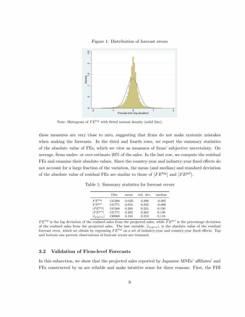
Figure 1: Distribution of forecast errors

0.5

11.

52

2.5

Den

sity

-2 -1 0 1 2Forecast error (log deviation)

Note: Histogram of FElog with fitted normal density (solid line).

these measures are very close to zero, suggesting that firms do not make systemic mistakes

when making the forecasts. In the third and fourth rows, we report the summary statistics

of the absolute value of FEs, which we view as measures of firms’ subjective uncertainty. On

average, firms under- or over-estimate 20% of the sales. In the last row, we compute the residual

FEs and examine their absolute values. Since the country-year and industry-year fixed effects do

not account for a large fraction of the variation, the mean (and median) and standard deviation

of the absolute value of residual FEs are similar to those of∣∣FElog

∣∣ and∣∣FEpct∣∣.

Table 1: Summary statistics for forecast errors

Obs. mean std. dev. median

FElog 131268 -0.025 0.299 -0.005FEpct 131771 0.016 0.332 -0.006|FElog | 131268 0.200 0.224 0.130|FEpct| 131771 0.203 0.263 0.130|εFElog | 130968 0.184 0.213 0.116

FElog is the log deviation of the realized sales from the projected sales, while FEpct is the percentage deviationof the realized sales from the projected sales. The last variable, |εFElog |, is the absolute value of the residualforecast error, which we obtain by regressing FElog on a set of industry-year and country-year fixed effects. Topand bottom one percent observations of forecast errors are trimmed.

3.2 Validation of Firm-level Forecasts

In this subsection, we show that the projected sales reported by Japanese MNEs’ affiliates’ and

FEs constructed by us are reliable and make intuitive sense for three reasons. First, the FDI

9

survey is mandated by METI and not imposed by the parent firms of these affiliates. As a

result, the affiliate reports the projected sales to the government and not to the parent firm.

Therefore, the strategic communication is not likely to be a concern here.17 Second, we show

that the projected sales have statistically significant and economically strong impact on realized

sales, employment and investment in the future. Specifically, we regress the realized sales (or

employment or investment) in year t on projected sales in year t− 1 (for sales in year t), lagged

sales in year t − 1 and t − 2 and a set of fixed effects. Robustly, we find that sales forecast

not only positively and statistically significantly affects on realized sales (and employment and

investment), but also has much stronger predictive power than the realized sales in previous

years. This empirical result verifies the reliability and usefulness of the information on firm-level

sales forecast.18

Finally, we show that the constructed FEs are positively correlated with aggregate-level

risk or volatility such as the Country Risk Index (from the BMI research database) and the

standard deviation of real GDP growth rates, which makes intuitive sense. In total, the empirical

regularities described in Appendix reassure us that the projected forecast for sales provided by

the Japanese affiliates abroad and the constructed FEs contain reliable and useful information

concerning micro-level uncertainty. In the next three subsections, we examine how firm-level

uncertainty gets resolved over the firm’s life cycle and how it is related to the parent firms’

previous export experience. Moreover, we present key evidence that substantiates the existence

of imperfect information in the international market, which cannot be rationalized by FIRE

models.19

3.3 Fact 1: Uncertainty Declines over Affiliates’ Life Cycle

In this subsection, we discuss how affiliates’ subjective uncertainty regarding future sales evolves

over their life cycles. We measure subjective uncertainty using the absolute value of FEs. Table

2 shows the simple average of affiliates’∣∣FElog

∣∣. As affiliates grow from age one to age seven,

their FEs decline from 36% to 18%, which means they are better at predicting future sales as

they become older. Similar patterns emerge when we consider alternative measures of FE.

We further confirm these patterns formally by estimating an OLS regression of affiliate i’s

FE in year t

|FElog|it = δt + βXit + δct + δs + εit,

17Specifically, the affiliate should not have the incentive to over-report the projected sales in order to impressthe parent firm.

18If the affiliates randomly or non-rationally reported their projected sales, the projected sales should have noor weak predictable power for future sales, employment and investment.

19For details, see Appendix 7.1.

10

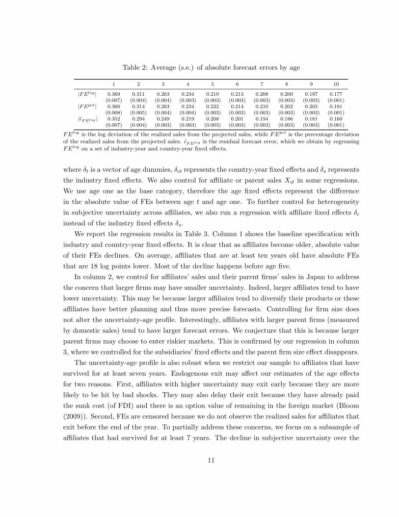
Table 2: Average (s.e.) of absolute forecast errors by age

1 2 3 4 5 6 7 8 9 10

|FElog | 0.369 0.311 0.263 0.234 0.219 0.213 0.208 0.200 0.197 0.177(0.007) (0.004) (0.004) (0.003) (0.003) (0.003) (0.003) (0.003) (0.003) (0.001)

|FEpct| 0.366 0.314 0.263 0.234 0.222 0.214 0.210 0.202 0.203 0.181(0.008) (0.005) (0.004) (0.004) (0.003) (0.003) (0.003) (0.003) (0.003) (0.001)

|εFElog | 0.352 0.294 0.249 0.219 0.208 0.201 0.194 0.186 0.181 0.160(0.007) (0.004) (0.003) (0.003) (0.003) (0.003) (0.003) (0.003) (0.003) (0.001)

FElog is the log deviation of the realized sales from the projected sales, while FEpct is the percentage deviationof the realized sales from the projected sales. εFElog is the residual forecast error, which we obtain by regressingFElog on a set of industry-year and country-year fixed effects.

where δt is a vector of age dummies, δct represents the country-year fixed effects and δs represents

the industry fixed effects. We also control for affiliate or parent sales Xit in some regressions.

We use age one as the base category, therefore the age fixed effects represent the difference

in the absolute value of FEs between age t and age one. To further control for heterogeneity

in subjective uncertainty across affiliates, we also run a regression with affiliate fixed effects δi

instead of the industry fixed effects δs.

We report the regression results in Table 3. Column 1 shows the baseline specification with

industry and country-year fixed effects. It is clear that as affiliates become older, absolute value

of their FEs declines. On average, affiliates that are at least ten years old have absolute FEs

that are 18 log points lower. Most of the decline happens before age five.

In column 2, we control for affiliates’ sales and their parent firms’ sales in Japan to address

the concern that larger firms may have smaller uncertainty. Indeed, larger affiliates tend to have

lower uncertainty. This may be because larger affiliates tend to diversify their products or these

affiliates have better planning and thus more precise forecasts. Controlling for firm size does

not alter the uncertainty-age profile. Interestingly, affiliates with larger parent firms (measured

by domestic sales) tend to have larger forecast errors. We conjecture that this is because larger

parent firms may choose to enter riskier markets. This is confirmed by our regression in column

3, where we controlled for the subsidiaries’ fixed effects and the parent firm size effect disappears.

The uncertainty-age profile is also robust when we restrict our sample to affiliates that have

survived for at least seven years. Endogenous exit may affect our estimates of the age effects

for two reasons. First, affiliates with higher uncertainty may exit early because they are more

likely to be hit by bad shocks. They may also delay their exit because they have already paid

the sunk cost (of FDI) and there is an option value of remaining in the foreign market (Bloom

(2009)). Second, FEs are censored because we do not observe the realized sales for affiliates that

exit before the end of the year. To partially address these concerns, we focus on a subsample of

affiliates that had survived for at least 7 years. The decline in subjective uncertainty over the

11

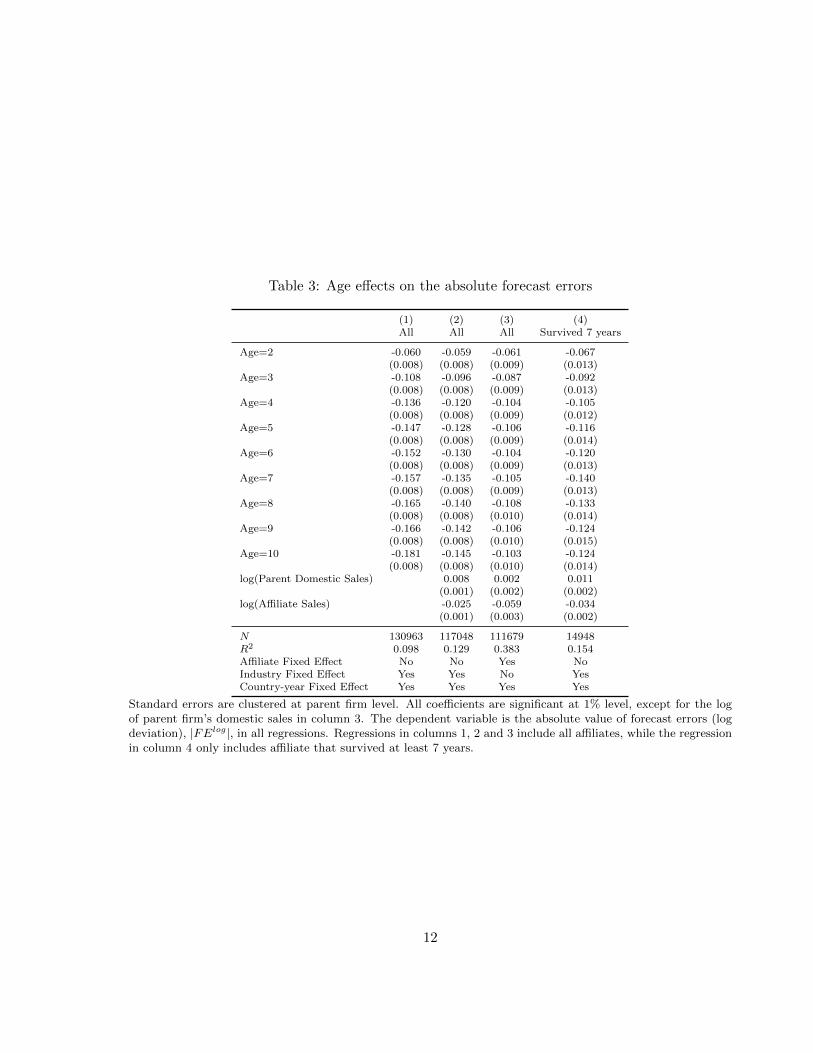
Table 3: Age effects on the absolute forecast errors

(1) (2) (3) (4)All All All Survived 7 years

Age=2 -0.060 -0.059 -0.061 -0.067(0.008) (0.008) (0.009) (0.013)

Age=3 -0.108 -0.096 -0.087 -0.092(0.008) (0.008) (0.009) (0.013)

Age=4 -0.136 -0.120 -0.104 -0.105(0.008) (0.008) (0.009) (0.012)

Age=5 -0.147 -0.128 -0.106 -0.116(0.008) (0.008) (0.009) (0.014)

Age=6 -0.152 -0.130 -0.104 -0.120(0.008) (0.008) (0.009) (0.013)

Age=7 -0.157 -0.135 -0.105 -0.140(0.008) (0.008) (0.009) (0.013)

Age=8 -0.165 -0.140 -0.108 -0.133(0.008) (0.008) (0.010) (0.014)

Age=9 -0.166 -0.142 -0.106 -0.124(0.008) (0.008) (0.010) (0.015)

Age=10 -0.181 -0.145 -0.103 -0.124(0.008) (0.008) (0.010) (0.014)

log(Parent Domestic Sales) 0.008 0.002 0.011(0.001) (0.002) (0.002)

log(Affiliate Sales) -0.025 -0.059 -0.034(0.001) (0.003) (0.002)

N 130963 117048 111679 14948R2 0.098 0.129 0.383 0.154Affiliate Fixed Effect No No Yes NoIndustry Fixed Effect Yes Yes No YesCountry-year Fixed Effect Yes Yes Yes Yes

Standard errors are clustered at parent firm level. All coefficients are significant at 1% level, except for the logof parent firm’s domestic sales in column 3. The dependent variable is the absolute value of forecast errors (logdeviation), |FElog|, in all regressions. Regressions in columns 1, 2 and 3 include all affiliates, while the regressionin column 4 only includes affiliate that survived at least 7 years.

12

firm’s life cycle is only slightly smaller than column 2, indicating that the forces discussed above

might be small in the data.

3.4 Fact 2: Learning about Market Demand through Exporting

In this subsection, we show that for affiliates that enter the destination country for the first time,

they face lower subjective uncertainty if their parent firms have previous export experience to

the region. The reduction in subjective uncertainty is economically significant compared to the

average subjective uncertainty faced by entering affiliates and to the overall decline of affiliates’

subjective uncertainty over time.

We restrict our sample to first-time entrants into countries or regions that we identify using

the founding year of the affiliates. We focus on affiliates in either the manufacturing sector or

the wholesale and retail sector whose parent firms are in manufacturing. Following Conconi et

al. (2016), we include distribution-oriented FDI such as wholesale and retail in our analysis since

affiliates in these industries may sell the same products as what the parent firms had previously

exported. As a result, previous export experience helps reduce demand uncertainty for these

distribution-oriented affiliates as well. We obtain information on parent firms’ previous export

experience using the firm survey data, which is at the region level.20 Using export information

at the regional level introduces additional measurement errors into our proxy for the export

experience and can lead to attenuation bias in our regressions. One can see the estimates as a

lower bound for the reduction in firm-level subjective uncertainty due to previous exporting.

We define previous export experience following a similar approach as in Conconi et al. (2016)

and Deseatnicov and Kucheryavyy (2017). Due to the lumpiness in international trade, we

define export entry if the firm does not export to the region for two consecutive years and starts

exporting afterwards (the variable of Exp Expe. used in Table 5). Similarly, we define export

exit if the firm stops exporting to the region for two consecutive years. For firms that have

begun to export but have not exited yet, their previous export experience is positive and defined

as the number of years since export entry. We assign zero year of export experience to firms that

have exited. In our main regression analysis, we show that our results are robust to alternative

measures of previous export experience.

Comparing to existing studies of first-time entrants of Japanese MNEs (Deseatnicov and

Kucheryavyy (2017)), our sample has fewer observations (see Table 4). The main reason is that

we only include first-time entrants that report sales at age two and projected sales at age one.

However, we obtain very similar patterns regarding exporting and affiliate entry. The majority

20Ideally, we would like to have export information at the country level, and explore how previous exports toparticular countries affect affiliates’ subjective uncertainty in those countries.

13

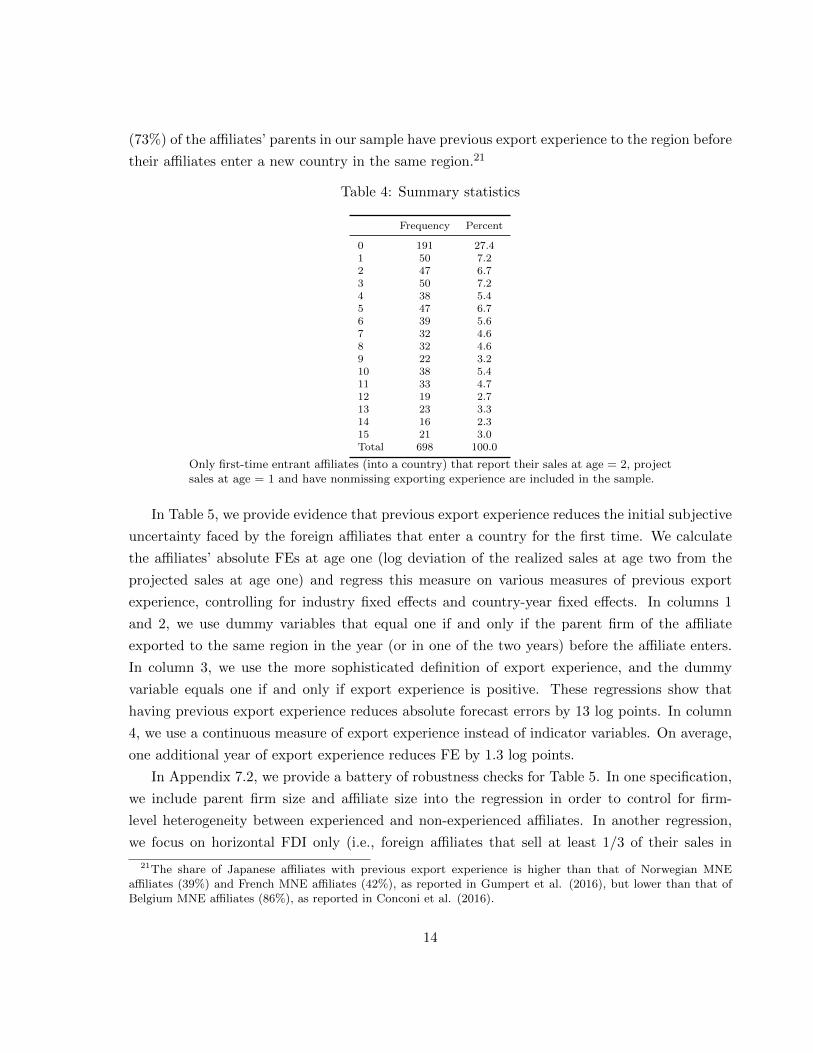
(73%) of the affiliates’ parents in our sample have previous export experience to the region before

their affiliates enter a new country in the same region.21

Table 4: Summary statistics

Frequency Percent

0 191 27.41 50 7.22 47 6.73 50 7.24 38 5.45 47 6.76 39 5.67 32 4.68 32 4.69 22 3.210 38 5.411 33 4.712 19 2.713 23 3.314 16 2.315 21 3.0Total 698 100.0

Only first-time entrant affiliates (into a country) that report their sales at age = 2, projectsales at age = 1 and have nonmissing exporting experience are included in the sample.

In Table 5, we provide evidence that previous export experience reduces the initial subjective

uncertainty faced by the foreign affiliates that enter a country for the first time. We calculate

the affiliates’ absolute FEs at age one (log deviation of the realized sales at age two from the

projected sales at age one) and regress this measure on various measures of previous export

experience, controlling for industry fixed effects and country-year fixed effects. In columns 1

and 2, we use dummy variables that equal one if and only if the parent firm of the affiliate

exported to the same region in the year (or in one of the two years) before the affiliate enters.

In column 3, we use the more sophisticated definition of export experience, and the dummy

variable equals one if and only if export experience is positive. These regressions show that

having previous export experience reduces absolute forecast errors by 13 log points. In column

4, we use a continuous measure of export experience instead of indicator variables. On average,

one additional year of export experience reduces FE by 1.3 log points.

In Appendix 7.2, we provide a battery of robustness checks for Table 5. In one specification,

we include parent firm size and affiliate size into the regression in order to control for firm-

level heterogeneity between experienced and non-experienced affiliates. In another regression,

we focus on horizontal FDI only (i.e., foreign affiliates that sell at least 1/3 of their sales in

21The share of Japanese affiliates with previous export experience is higher than that of Norwegian MNEaffiliates (39%) and French MNE affiliates (42%), as reported in Gumpert et al. (2016), but lower than that ofBelgium MNE affiliates (86%), as reported in Conconi et al. (2016).

14

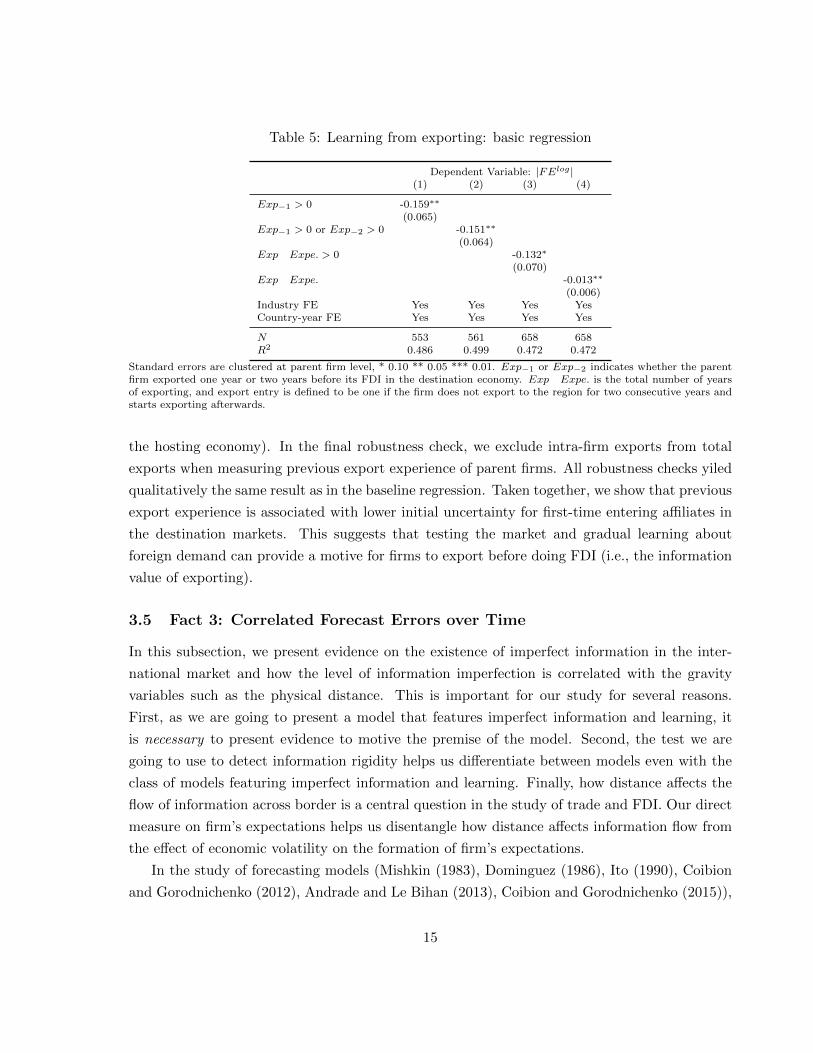
Table 5: Learning from exporting: basic regression

Dependent Variable: |FElog |(1) (2) (3) (4)

Exp−1 > 0 -0.159∗∗

(0.065)Exp−1 > 0 or Exp−2 > 0 -0.151∗∗

(0.064)Exp Expe. > 0 -0.132∗

(0.070)Exp Expe. -0.013∗∗

(0.006)Industry FE Yes Yes Yes YesCountry-year FE Yes Yes Yes Yes

N 553 561 658 658R2 0.486 0.499 0.472 0.472

Standard errors are clustered at parent firm level, * 0.10 ** 0.05 *** 0.01. Exp−1 or Exp−2 indicates whether the parentfirm exported one year or two years before its FDI in the destination economy. Exp Expe. is the total number of yearsof exporting, and export entry is defined to be one if the firm does not export to the region for two consecutive years andstarts exporting afterwards.

the hosting economy). In the final robustness check, we exclude intra-firm exports from total

exports when measuring previous export experience of parent firms. All robustness checks yiled

qualitatively the same result as in the baseline regression. Taken together, we show that previous

export experience is associated with lower initial uncertainty for first-time entering affiliates in

the destination markets. This suggests that testing the market and gradual learning about

foreign demand can provide a motive for firms to export before doing FDI (i.e., the information

value of exporting).

3.5 Fact 3: Correlated Forecast Errors over Time

In this subsection, we present evidence on the existence of imperfect information in the inter-

national market and how the level of information imperfection is correlated with the gravity

variables such as the physical distance. This is important for our study for several reasons.

First, as we are going to present a model that features imperfect information and learning, it

is necessary to present evidence to motive the premise of the model. Second, the test we are

going to use to detect information rigidity helps us differentiate between models even with the

class of models featuring imperfect information and learning. Finally, how distance affects the

flow of information across border is a central question in the study of trade and FDI. Our direct

measure on firm’s expectations helps us disentangle how distance affects information flow from

the effect of economic volatility on the formation of firm’s expectations.

In the study of forecasting models (Mishkin (1983), Dominguez (1986), Ito (1990), Coibion

and Gorodnichenko (2012), Andrade and Le Bihan (2013), Coibion and Gorodnichenko (2015)),

15

whether FEs made in different periods are correlated is used to detect the existence of informa-

tion rigidity.22 Intuitively, as FIRE models imply that agents have perfect information, errors

made by the forecast in the current period (for the values of variable in the next period) are all

caused by unexpected and contemporaneous shocks that happen next period (i.e., innovations in

the next period). Thus, FEs made at two different periods are serially uncorrelated in FIRE

models, as the unexpectedly contemporaneous shocks are uncorrelated by definition. Therefore,

if the data of FEs exhibit serial correlation between FEs made in two different periods, we can

confidently reject the null hypothesis that agents know information perfectly. Moreover, the va-

lidity of this test is robust to different functional form and distributional assumptions we make

in the model (e.g., whether the variance of the contemporaneous shock is age dependent and

whether the fundamental shock is log normal). In total, the test on the serial correlation of FEs

made in different periods provides direct and clean evidence for the existence of information

rigidity.

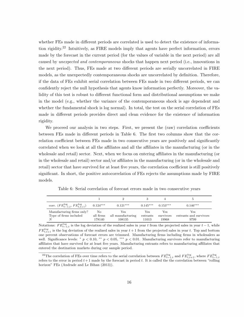
We proceed our analysis in two steps. First, we present the (raw) correlation coefficients

between FEs made in different periods in Table 6. The first two columns show that the cor-

relation coefficient between FEs made in two consecutive years are positively and significantly

correlated when we look at all the affiliates and all the affiliates in the manufacturing (or in the

wholesale and retail) sector. Next, when we focus on entering affiliates in the manufacturing (or

in the wholesale and retail) sector and/or affiliates in the manufacturing (or in the wholesale and

retail) sector that have survived for at least five years, the correlation coefficient is still positively

significant. In short, the positive autocorrelation of FEs rejects the assumptions made by FIRE

models.

Table 6: Serial correlation of forecast errors made in two consecutive years

1 2 3 4 5

corr. (FElogt−1,t, FE

logt,t+1) 0.124∗∗∗ 0.121∗∗∗ 0.145∗∗∗ 0.153∗∗∗ 0.146∗∗∗

Manufacturing firms only? No Yes Yes Yes YesType of firms included all firms all manufacturing entrants survivors entrants and survivorsN 178140 108135 11013 19968 9799

Notations: FElogt−1,t is the log deviation of the realized sales in year t from the projected sales in year t− 1, while

FElogt,t+1 is the log deviation of the realized sales in year t+ 1 from the projected sales in year t. Top and bottomone percent observations of forecast errors are trimmed. Manufacturing firms including firms in wholesalers aswell. Significance levels: ∗ p < 0.10, ∗∗ p < 0.05, ∗∗∗ p < 0.01. Manufacturing survivors refer to manufacturingaffiliates that have survived for at least five years. Manufacturing entrants refers to manufacturing affiliates thatentered the destination markets during our sample period.

22The correlation of FEs over time refers to the serial correlation between FElogt−1,t and FElog

t,t+1, where FElogt−1,t

refers to the error in period t+ 1 made by the forecast in period t. It is called the the correlation between “rollinghorizon” FEs (Andrade and Le Bihan (2013)).

16

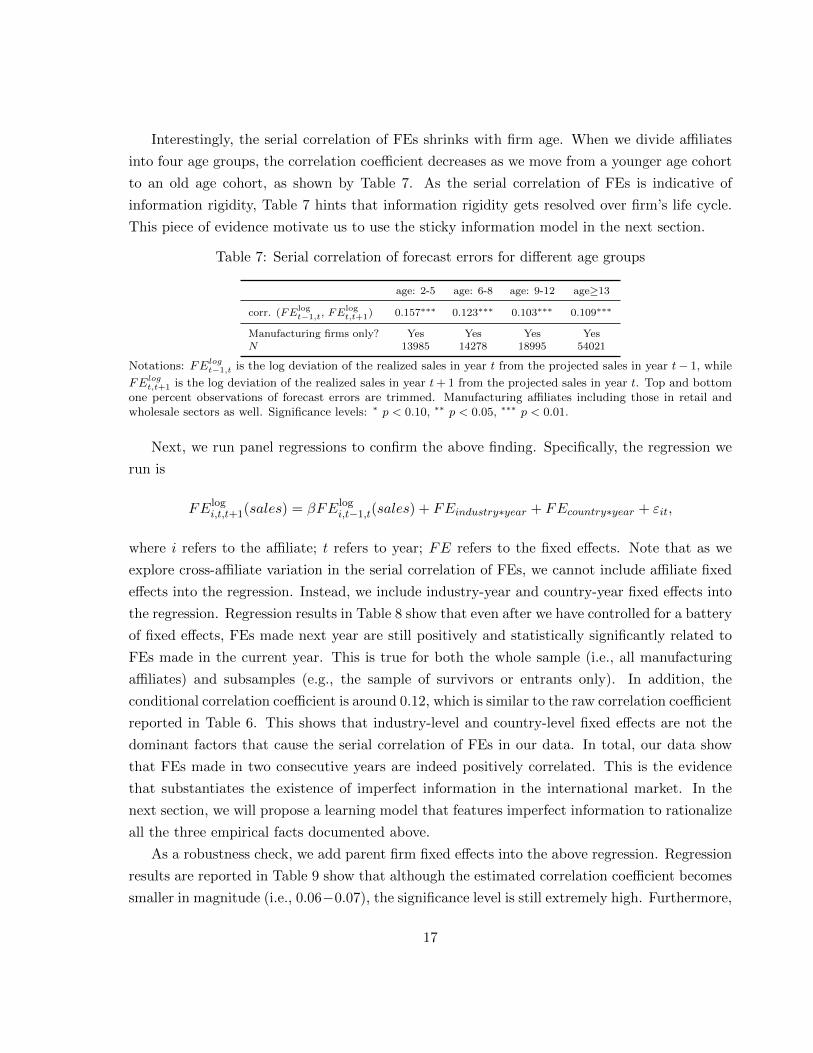
Interestingly, the serial correlation of FEs shrinks with firm age. When we divide affiliates

into four age groups, the correlation coefficient decreases as we move from a younger age cohort

to an old age cohort, as shown by Table 7. As the serial correlation of FEs is indicative of

information rigidity, Table 7 hints that information rigidity gets resolved over firm’s life cycle.

This piece of evidence motivate us to use the sticky information model in the next section.

Table 7: Serial correlation of forecast errors for different age groups

age: 2-5 age: 6-8 age: 9-12 age≥13

corr. (FElogt−1,t, FE

logt,t+1) 0.157∗∗∗ 0.123∗∗∗ 0.103∗∗∗ 0.109∗∗∗

Manufacturing firms only? Yes Yes Yes YesN 13985 14278 18995 54021

Notations: FElogt−1,t is the log deviation of the realized sales in year t from the projected sales in year t− 1, while

FElogt,t+1 is the log deviation of the realized sales in year t+ 1 from the projected sales in year t. Top and bottomone percent observations of forecast errors are trimmed. Manufacturing affiliates including those in retail andwholesale sectors as well. Significance levels: ∗ p < 0.10, ∗∗ p < 0.05, ∗∗∗ p < 0.01.

Next, we run panel regressions to confirm the above finding. Specifically, the regression we

run is

FElogi,t,t+1(sales) = βFElog

i,t−1,t(sales) + FEindustry∗year + FEcountry∗year + εit,

where i refers to the affiliate; t refers to year; FE refers to the fixed effects. Note that as we

explore cross-affiliate variation in the serial correlation of FEs, we cannot include affiliate fixed

effects into the regression. Instead, we include industry-year and country-year fixed effects into

the regression. Regression results in Table 8 show that even after we have controlled for a battery

of fixed effects, FEs made next year are still positively and statistically significantly related to

FEs made in the current year. This is true for both the whole sample (i.e., all manufacturing

affiliates) and subsamples (e.g., the sample of survivors or entrants only). In addition, the

conditional correlation coefficient is around 0.12, which is similar to the raw correlation coefficient

reported in Table 6. This shows that industry-level and country-level fixed effects are not the

dominant factors that cause the serial correlation of FEs in our data. In total, our data show

that FEs made in two consecutive years are indeed positively correlated. This is the evidence

that substantiates the existence of imperfect information in the international market. In the

next section, we will propose a learning model that features imperfect information to rationalize

all the three empirical facts documented above.

As a robustness check, we add parent firm fixed effects into the above regression. Regression

results are reported in Table 9 show that although the estimated correlation coefficient becomes

smaller in magnitude (i.e., 0.06−0.07), the significance level is still extremely high. Furthermore,

17

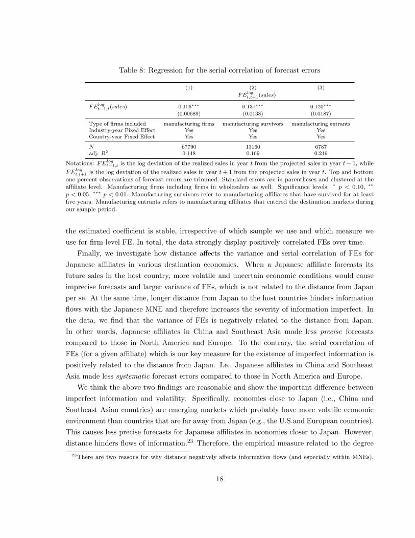
Table 8: Regression for the serial correlation of forecast errors

(1) (2) (3)

FElogt,t+1(sales)

FElogt−1,t(sales) 0.106∗∗∗ 0.131∗∗∗ 0.120∗∗∗

(0.00689) (0.0138) (0.0187)

Type of firms included manufacturing firms manufacturing survivors manufacturing entrantsIndustry-year Fixed Effect Yes Yes YesCountry-year Fixed Effect Yes Yes Yes

N 67790 13160 6787adj. R2 0.148 0.169 0.219

Notations: FElogt−1,t is the log deviation of the realized sales in year t from the projected sales in year t− 1, while

FElogt,t+1 is the log deviation of the realized sales in year t+ 1 from the projected sales in year t. Top and bottomone percent observations of forecast errors are trimmed. Standard errors are in parentheses and clustered at theaffiliate level. Manufacturing firms including firms in wholesalers as well. Significance levels: ∗ p < 0.10, ∗∗

p < 0.05, ∗∗∗ p < 0.01. Manufacturing survivors refer to manufacturing affiliates that have survived for at leastfive years. Manufacturing entrants refers to manufacturing affiliates that entered the destination markets duringour sample period.

the estimated coefficient is stable, irrespective of which sample we use and which measure we

use for firm-level FE. In total, the data strongly display positively correlated FEs over time.

Finally, we investigate how distance affects the variance and serial correlation of FEs for

Japanese affiliates in various destination economies. When a Japanese affiliate forecasts its

future sales in the host country, more volatile and uncertain economic conditions would cause

imprecise forecasts and larger variance of FEs, which is not related to the distance from Japan

per se. At the same time, longer distance from Japan to the host countries hinders information

flows with the Japanese MNE and therefore increases the severity of information imperfect. In

the data, we find that the variance of FEs is negatively related to the distance from Japan.

In other words, Japanese affiliates in China and Southeast Asia made less precise forecasts

compared to those in North America and Europe. To the contrary, the serial correlation of

FEs (for a given affiliate) which is our key measure for the existence of imperfect information is

positively related to the distance from Japan. I.e., Japanese affiliates in China and Southeast

Asia made less systematic forecast errors compared to those in North America and Europe.

We think the above two findings are reasonable and show the important difference between

imperfect information and volatility. Specifically, economies close to Japan (i.e., China and

Southeast Asian countries) are emerging markets which probably have more volatile economic

environment than countries that are far away from Japan (e.g., the U.S.and European countries).

This causes less precise forecasts for Japanese affiliates in economies closer to Japan. However,

distance hinders flows of information.23 Therefore, the empirical measure related to the degree

23There are two reasons for why distance negatively affects information flows (and especially within MNEs).

18

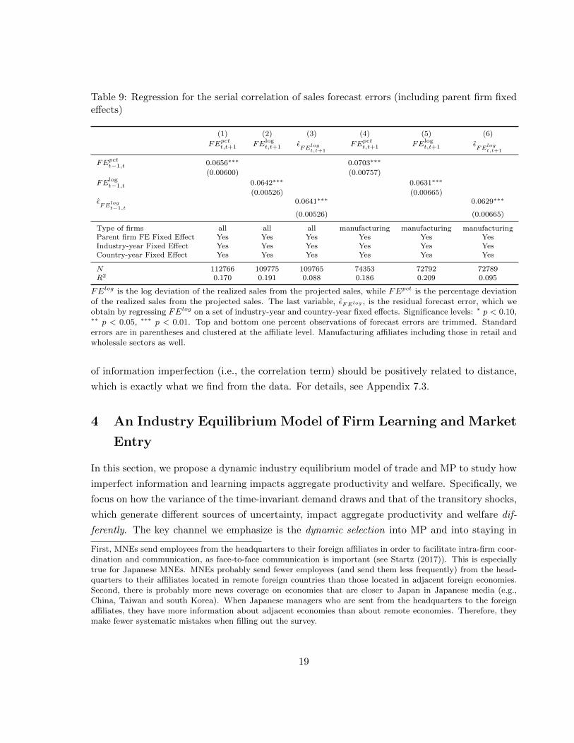
Table 9: Regression for the serial correlation of sales forecast errors (including parent firm fixedeffects)

(1) (2) (3) (4) (5) (6)

FEpctt,t+1 FElogt,t+1 ε

FElogt,t+1

FEpctt,t+1 FElogt,t+1 ε

FElogt,t+1

FEpctt−1,t 0.0656∗∗∗ 0.0703∗∗∗

(0.00600) (0.00757)

FElogt−1,t 0.0642∗∗∗ 0.0631∗∗∗

(0.00526) (0.00665)εFE

logt−1,t

0.0641∗∗∗ 0.0629∗∗∗

(0.00526) (0.00665)

Type of firms all all all manufacturing manufacturing manufacturingParent firm FE Fixed Effect Yes Yes Yes Yes Yes YesIndustry-year Fixed Effect Yes Yes Yes Yes Yes YesCountry-year Fixed Effect Yes Yes Yes Yes Yes Yes

N 112766 109775 109765 74353 72792 72789R2 0.170 0.191 0.088 0.186 0.209 0.095

FElog is the log deviation of the realized sales from the projected sales, while FEpct is the percentage deviationof the realized sales from the projected sales. The last variable, εFElog , is the residual forecast error, which weobtain by regressing FElog on a set of industry-year and country-year fixed effects. Significance levels: ∗ p < 0.10,∗∗ p < 0.05, ∗∗∗ p < 0.01. Top and bottom one percent observations of forecast errors are trimmed. Standarderrors are in parentheses and clustered at the affiliate level. Manufacturing affiliates including those in retail andwholesale sectors as well.

of information imperfection (i.e., the correlation term) should be positively related to distance,

which is exactly what we find from the data. For details, see Appendix 7.3.

4 An Industry Equilibrium Model of Firm Learning and Market

Entry

In this section, we propose a dynamic industry equilibrium model of trade and MP to study how

imperfect information and learning impacts aggregate productivity and welfare. Specifically, we

focus on how the variance of the time-invariant demand draws and that of the transitory shocks,

which generate different sources of uncertainty, impact aggregate productivity and welfare dif-

ferently. The key channel we emphasize is the dynamic selection into MP and into staying in

First, MNEs send employees from the headquarters to their foreign affiliates in order to facilitate intra-firm coor-dination and communication, as face-to-face communication is important (see Startz (2017)). This is especiallytrue for Japanese MNEs. MNEs probably send fewer employees (and send them less frequently) from the head-quarters to their affiliates located in remote foreign countries than those located in adjacent foreign economies.Second, there is probably more news coverage on economies that are closer to Japan in Japanese media (e.g.,China, Taiwan and south Korea). When Japanese managers who are sent from the headquarters to the foreignaffiliates, they have more information about adjacent economies than about remote economies. Therefore, theymake fewer systematic mistakes when filling out the survey.

19

the market (i.e., exporting or MP). In the counterfactual exercise, We find that an increase in

the variance of the transitory demand shocks reduces aggregate productivity and welfare, while

an increase in the variance of the time-invariant demand draws increases them.

Economically speaking, MP is a more productive technology than exporting, as it helps firms

save on the variable cost and requires one-time sunk costs. Furthermore, firms with good time-

invariant demand draws would stay in the market if there were no imperfect information. Due to

the existence of imperfect information, firms that do MP are not necessarily those with the best

time-invariant demand draws, and firms that exit are not necessarily those with the worst time-

invariant demand draws in the economy. An increase in the variance of the transitory demand

shocks reduces the signal-to-noise ratio and the effectiveness of learning. As a result, such an

increase prevents the economy from allocating the most efficient firms to do FDI and the least

efficient firms to exit, which leads to lower aggregate productivity and welfare. To the contrary,

an increase in the variance of the time-invariant demand draws increases the effectiveness of

learning, and therefore helps the economy select the most efficient firms to do FDI and the least

efficient firms to exit.

We build up a dynamic industry equilibrium model of heterogeneous firms a la Arkolakis

et al. (2017) to rationalize the empirical findings documented above. Similar to Arkolakis et

al. (2017), the firm learns about its fundamental foreign demand by selling its products in

the destination market. Different from Arkolakis et al. (2017) (and also Jovanovic (1982)), we

allow the firm to make an endogenous and dynamics choice on its entry model into the foreign

market (i.e., exporting v.s. MP). In particular, the firm can export its products to the foreign

market before setting up an affiliate there, as exporting entails smaller sunk costs and generates

information value. In addition, we introduce sticky information a la Mankiw and Reis (2002)

into the Jovanovic-type firm dynamics model (Jovanovic (1982)) in order to match the positive

serial correlation of FEs observed in the data. The spirit of our model is close to the two-period

model studied in Conconi et al. (2016). However, we make key departures from Conconi et

al. (2016) by focusing on the difference between the two types of shocks the firm faces and by

emphasizing the life cycle feature of uncertainty and information imperfection at the firm level.

4.1 Setup: Demand and Supply

This section considers a dynamic industry equilibrium model in which each Japanese firm pro-

duces a differentiated variety and has to decide between exporting and FDI in order to serve the

foreign country (i.e., the rest of the world). For simplicity and the data constraint, we abstract

from Japanese firms’ domestic activities and focus on their overseas activities only. Specifically,

the total expenditure of foreign consumers is assumed to be fixed and exogenous to Japanese

20

firms’ activities in the foreign market. This is a reasonable assumption, as Japanese products

(Japanese MNEs’ local sales plus Japanese exports) only account for a small share of the total

consumption in any major economy in the world (e.g., the U.S., China, E.U. etc.). Therefore,

Japanese exports and its MNEs’ activities should generate small general equilibrium effects in

destination countries. Labor is the only input in production. We assume that Japanese affiliates

only employ a small fraction of the labor force in destination economies and therefore cannot

affect the wage there. In addition, we also abstract from the analysis on how trade and FDI

affect the domestic labor market in Japan and assume domestic wage is fixed.

We introduce the demand side structure of the model. In the foreign country, the representa-

tive consumer has the following nested-CES preferences where the first nest is among composite

goods produced by firms from different countries, indexed by i,

Ut =

(∑i

χ1δi Q

δ−1δ

it

) δδ−1

,

and the second nest is among varieties ω ∈ Σit produced by firms from each country i,

Qit =

(∫ω∈Σit

eat(ω)σ qt(ω)

σ−1σ dω

) σσ−1

. (1)

In the first nest, the parameter χi is the demand shifter for country i goods, and the parameter

δ is the Armington elasticity between goods produced by firms from different countries. In

the second nest, the parameter σ is the elasticity between different varieties, and at (ω) is the

demand shifter for variety ω. We assume that firms differ in their demand shifter, at (ω).

After denoting foreign consumers’ total expenditure as Yt, we can express the demand for a

particular Japanese variety, ω, as:

qt(ω) =Yt

P 1−δt

χjpPσ−δjp,t e

at(ω)pt(ω)−σ, (2)

where Pt is the aggregate price index for all goods, and Pjp,t is the ideal price index for Japanese

goods. When the Armington elasticity δ equals 1, the first nest is Cobb-Douglas, and the

expenditure on Japanese goods no longer depend on Pjp,t. When σ = δ, the elasticities in the

two CES nests are the same, which is the case in prominent trade models such as Eaton and

Kortum (2002) and Melitz (2003). In our calibration, we set δ to be a value between 1 and σ.

In our industry equilibrium model, we treat Yt and Pt as exogenous. Therefore, we combine

the exogenous terms in expression (2), YtPδ−1t χjp into one variable, Yt, and call it the aggregate

21

demand shifter. In addition, since we only focus on Japanese firms, we suppress the subscript jp

in the following analysis. The CES preference over different varieties of Japanese goods implies

the ideal price index as:

Pt ≡(∫

ω∈Σt

eat(ω)pt(ω)1−σdω

)1/(1−σ)

. (3)

We use the term, At ≡ YtPσ−δt to denote the aggregate demand condition faced by all firms in

period t and rewrite the firm-level demand function as

qt(ω) = Ateat(ω)pt(ω)−σ. (4)

We specify firm-level behavior in what follows. First, we assume that demand uncertainty

comes from the firm-specific demand shifter, at (ω), for each firm. Specifically, Japanese firms

differ in the firm-specific demand shift, at (ω), and we assume that at (ω) is the sum of a time-

invariant fundamental demand draw θ (ω) and a transitory shock εt (ω) as in Jovanovic (1982)

and Arkolakis et al. (2017):

at (ω) = θ (ω) + εt(ω), εt(ω)i.i.d.∼ N

(0, σ2

ε

). (5)

Firms understand that θ (ω) is drawn from a normal distribution N(θ, σ2

θ

), and the indepen-

dent and identically distributed (i.i.d.) transitory shock, εt (ω), is drawn from another normal

distribution N(0, σ2

ε

). Importantly, we assume that the firm does not know the value of its time-

invariant demand draw. Each period, although the firm observes the realize demand, θ (ω), it

cannot distinguish between θ (ω) and εt(ω). Instead, the firm forms an posterior belief about

the distribution of θ.

Next, we assume that there are two types of firms in the economy in the same spirit as in

sticky information models a la Mankiw and Reis (2002): the informed firms and the uninformed

firms. Initially, all entering firms are uninformed in the sense that they all use the prior distri-

bution of θ (i.e., N(θ, σ2θ)) to form the expectation for the fundamental demand draw. At the

end of each period, 1−α fraction of the remaining uninformed firms become informed. From the

time when they become informed, they begin to update the beliefs for θ(ω) by utilizing realized

overall demand shocks and will never become uninformed again. The remaining uninformed

firms still use the prior distribution of θ to make their forecasts. When time elapses, more and

more firms become informed, and all firms become informed when they live long enough.

Different from the demand side, we assume that firms are homogenous in labor productivity

for simplicity. Specifically, in order to produce q units of output, the firm has to employ the

22

same amount of workers. This simplification is motivated by recent work that emphasizes the

importance of demand heterogeneity for understanding firm heterogeneity (e.g., Hottman et al.

(2016)).

The industry structure is characterized by monopolistically competition. There is an exoge-

nous mass of potential entrants J (from Japan) that decide whether or not to enter the foreign

market every period. Each entrant draws a time-invariant demand shifter θ from a normal dis-

tribution, N(θ, σ2

θ

). Every entrant does not know its fundamental demand draw and has to use

the prior belief for θ to decide whether to enter the foreign market. If the firm chooses to enter

the market, it also has to decide how to serve the foreign market. A potential entrant can either

serve the foreign market via exporting, which involves a sunk cost of fex, or serve the foreign

market by setting up an affiliate with an entry cost of fem. Both sunk costs are paid in units

of domestic labor. If neither mode is profitable, the potential entrant simply exits and obtains

zero payoff.

Similar to entrants, incumbents do not know the exact value of θ. However, the informed

incumbents have better information for the fundamental demand than entrants, as they can

utilize information on past sales to update the beliefs for the fundamental demand draw. The

uninformed incumbents have the same information concerning the fundamental demand as the

entrants, as they have not figured out how to utilize information on past sales to update their

beliefs. In each period, the incumbents first receive an exogenous death shock with probability

η. For surviving firms, they have to decide whether to change their mode of service. They

can keep their service mode unchanged. Alternatively, they can switch to another mode of

service (i.e., from exporting to MP or from MP to exporting). In addition, they can also choose

to permanently exit the market. We assume that for exporters, they have to pay a one-time

entry cost, fex, in order to start exporting. However, incumbent MNEs can switch to exporting

without paying this sunk cost. Firms also have to pay a fixed cost each period in order to remain

exporting (with a fixed cost of fx) or doing FDI (with a fixed cost of fm). Therefore, firms with

low demand draws will choose to exit.

For firms that serve the foreign market, they decide how much to produce in period t before

the overall demand shock at is realized. After the overall demand shock in period t, at, is

realized, they choose the price pt in order to sell all the products they have produced, as there is

no storage technology and firms cannot accumulate inventories. For informed incumbent firms,

they update their beliefs about the fundamental demand θ after observing the overall demand

shock in period t: at. Additionally, a randomly selected 1 − α fraction of uninformed firms

become informed at the end of each period.

In the calibration exercise, we normalize the sunk entry cost into exporting, fex, to zero,

23

as we do not use the information on domestic production of Japanese firms to calibrate this

parameter. Additionally, we follow the literature on exporter/MP dynamics (Ruhl and Willis

(2016), Das et al. (2007) etc.) to assume that the sunk entry cost into FDI, fem, is drawn from a

log normal distribution. As a result, the sunk entry cost into FDI becomes a state variable for

the firm’s dynamic optimization decision.24 Finally, the fixed per-period operation cost of MP,

fm, is set to be zero, as there is a flat profile of exit rate (with firm age) over MNEs’ affiliates’

life cycles.

4.2 Belief Updating and Serially Correlated Forecast Errors

In this subsection, we show that our model of firm learning described above can rationalize all

the three empirical findings documented in Section 3. In particular, both FIRE models and the

original Jovanovic model (i.e., Jovanovic (1982)) do not yield positively correlated FEs overtime.

We proceed our analysis in the following three steps.

4.2.1 Full Information Rational Expectation Models

First, we show that FIRE models which assume that firms know their time-invariant demand

draws yield serially uncorrelated FEs, which are inconsistent with our empirical finding. Specif-

ically, as the firm knows its time-invariant demand shifter, θ (ω), in FIRE models, it chooses the

level of output to maximize:

maxqt

EεtA1σt e

θ+εtσ q

σ−1σ

t − wqt,

where w is the wage rate. Thus, the optimal output choice is

qt(θ) = Ateθ+

σ2ε

2σ

((σ − 1)

σw

)σ,

24Another reason for assuming that firms make random draws of the entry costs into FDI is to match theproductivity hierarchy among first-time entrants (into the destination markets) documented in Table 20. Thetable shows that experienced affiliates are more productive than non-experienced affiliates. In the model, non-experienced affiliates choose to enter the FDI market (after entry) based on the entry costs (i.e., not based onthe information concerning the fundamental demand draw), as all entrants have the same prior belief about thefundamental demand draw. In other words, the selection into FDI is random in the dimension of the fundamentaldemand draws for non-experienced affiliates. However, experienced affiliates are a selected sample of firms thathave better fundamental demand draws than the ex ante average, as only firms that have better ex post beliefsfor their fundamental demand draws choose to enter the FDI market. This leads to the theoretical predictionthat experienced affiliates are more productive than non-experienced affiliates in terms of revenue productivity,which is true in the data. If we introduce ex ante heterogeneity in labor productivity instead of the entry costinto FDI, non-experienced affiliates are also a selected sample of firms that have higher productivity than the exante average. Therefore, the productivity hierarchy pattern among first-time entrants cannot be rationalized bythe theory.

24

and the resulting FE is25

FElogt−1,t(sales) =

εtσ− σ2

ε

2σ2. (6)

It is clear that the covariance of FEs made in two consecutive periods is

cov(FElogt−1,t, FE

logt,t+1) = cov

(εtσ,εt+1

σ

)= 0,

as the transitory shock is uncorrelated over time. Moreover, even if the fundamental demand

draw, θ, is time-varying and follows an AR(m) processes (m = 1, 2, ...), we still have the result of

non-correlated FEs over time as the innovation in the demand process is unpredictable.26 This

result is true for FIRE models in general (see Mishkin (1983)). A final remark is that even if

we allow for the endogenous exit by firms over time, the implied serial correlation of FEs will

become negative. The detailed discussion is relegated to Appendix 6.2 which consider the case

in which the fundamental demand draw follows an AR(1) process. In total, FIRE models cannot

be used to rationalize the positively correlated of FEs over time observed in our data.

4.2.2 Jovanovic Model: Jovanovic (1982)

In this subsection, we discuss how the firm forms its ex post belief for the fundamental demand

draw in the Jovanoic model (Jovanovic (1982)), which is a special case of our full model with

α = 0. In the Jovanovic model, the firm does not directly observe its time-invariant demand

θ (ω), although it knows the prior distribution of θ(ω). In the beginning of period t+ 1, the firm

knows the realizations of the overall demand shifters up to period t,27 as it has observed t signals

before (i.e., a set of {ai}i=1,2...,t). Since both the prior distribution of θ and the distribution of

the noise ε are normal, the Bayes’ rule implies that the posterior belief about θ (after observing

t signals) is also normal with mean µt and variance σ2t , where

µt =σ2ε

σ2ε + tσ2

θ

θ +tσ2θ

σ2ε + tσ2

θ

at, (7)

25Readers are referred to Appendix 6.1 for the detail.26A digression here is that the first two empirical patterns documented above can be rationalized by the perfect

information model with age-dependent volatility. In particular, if the variance of the i.i.d. demand shock goesdown with firm age and market experience, older affiliates and affiliates whose parent firms have previous exportexperience have smaller variance and absolute value of FEs. However, even if we allow for age-dependent volatility,FIRE models still cannot rationalize the positive serial correlation between FEs, as this prediction is independentof distributional assumptions and functional form we impose on εt and on the demand/productivity processes.

27For age one firms, they do not know any realized overall demand shock, as they just enter the market.

25

and

σ2t =

σ2εσ

2θ

σ2ε + tσ2

θ

. (8)

The history of signals (a1, a2, . . . , at) is summarized by age t and the average

at ≡1

t

t∑i=1

ai for t ≥ 1; a0 ≡ θ.

Therefore, the firm believes that the overall demand shock at age t, at = θ + εt, has a normal

distribution with mean µt−1 and variance σ2t−1 + σ2

ε . For a firm of age t with previous history

at−1, (at−1, t) summarizes all necessary information concerning the firm’s belief about the value

of θ. For age one firm, its belief for the mean and variance of θ is the same as the prior beliefs.

Next, we state the firm’s optimization problem. The objective function now becomes

maxqt

Eθ,εtA1σt e

θ+εtσ q

σ−1σ

t − wqt,

which leads to the result that

qt = At

(σ − 1

σ

)σ (b (at−1, t− 1)

w

)σ, (9)

where

b (at−1, t− 1) = Eat|at−1,t−1

(eat/σ

)(10)

= exp

{µt−1

σ+

1

2

(σ2t−1 + σ2

ε

σ2

)}.

The next proposition shows that the FEs in two consecutive periods are uncorrelated:

Proposition 1 Forecast errors made in two consecutive periods by the same firm are uncorre-

lated.

Proof. See Appendix 6.6.

There are three components in the expression of FE that are correlated over time. First, there is

a positive correlation between θ− µt−1 and θ− µt, as both µt and µt−1) only contain a fraction

of the true θ.28 Second, the firm includes the i.i.d. shocks up to period t−1 (i.e., {εi}i=1,2,...t−1)

into the forecast made in both periods t− 1 and t. As these shocks do not affect the realization

28In other words, as the firm partially includes the true time-invariant demand into its forecast, there is adifference between the true time-invariant demand and the prior mean in the FE (i.e., (1 − ζ(t − 1, λ))(θ − θ))every period, which causes a positive correlation.

26

of the transitory demand shock after period t−1, this causes another positive correlation of FEs

over time. Finally, since the transitory shock in period t positively affects the FE in period t

and negatively affects the FE in period t+ 129, there is a negative correlation coming from the

transitory shock in period t (i.e., εt). This negative part of correlation perfectly cancels out the

(first two) positive parts of correlation, which leads to zero serial correlation of FEs over time.

Undoubtedly, this property is a result coming form the assumption that the learning object (i.e.,

θ) is fixed overtime. In Appendix 6.3, we show that even when the fundamental demand draw

follows a random walk over time, the serial correlation of FEs is not necessarily zero.

Although the Jovanovic model cannot generate the positive correlation of FEs over time, it

can explain the fact that the variance of FEs goes down with firm age and market experience.

Based on equation (42), we can derive the variance of FEs at age t as

var(FElogt−1,t(sales)) =

var(εt + θ − µt−1)

σ2

=var(εt) + var(θ) + var(µt−1)− 2cov(θ, µt−1)

σ2,

as εt is independent of θ and µt−1. The next proposition shows that this variance decreases with

firm age and previous experience in the market:

Proposition 2 Variance of the forecast errors declines with years of experience t.

Proof. See Appendix 6.6.1.

Thanks to the accumulation of experience, the variance of FEs (and the absolute value of FEs)

becomes smaller, when the affiliate becomes older and when the affiliate’s parent firm has export

experience to the region where the affiliate is set up afterwards. In summary, the Jovanovic

model can explain the first two empirical facts documented above, but not the third one. This

motivates us to extend the Jovanovic model at the minimum level to rationalize all the three

empirical findings.30

4.2.3 Learning Model with Information Rigidity

In this subsection, we show how our full model with α > 0 can rationalize all the three empirical

findings documented above. First, we use the following proposition to show that the modified

Jovanovic model presented in Subsection 4.1 still implies declining variance of FEs with firm

age and market experience.

29Remember that it enters into the firm’s experience when the firm make the forecast in period t+ 1.30Jovanovic model has implications for age-dependent volatility of growth rate of output. Specifically, the model

predicts that the volatility of growth rate of output decreases with firm age, which is a salient feature of our data.For details, see Appendix 6.4.

27

Proposition 3 Variance of the forecast errors declines with years of experience t.

Proof. See Appendix 6.6.2.

In the modified learning model, we have two forces that push down the imprecision of forecasts

over firm’s life cycle. First, informed firms accumulate more experience and have clearer infor-

mation about their fundamental demand, when they operate in the market for a longer period

of time. Next, as more firms become informed over time and informed firms make more accurate

forecasts (compared to the uninformed firms), the variance of FEs goes down with firm’s market

experience.31

Next, we characterize the serial correlation of FEs in our full model using the following

proposition:

Proposition 4 Forecast errors made in two consecutive periods by the same firm are positively

correlated.

Proof. See Appendix 6.6.3.

The above proposition rationalizes our last empirical finding concerning the positive correla-

tion between FEs made in two consecutive periods. First, FEs of informed firms are serially

uncorrelated, which is the same as in the Jovanovic model. Moreover, FEs of the switching

firms (i.e., firms that become informed during the two periods) are uncorrelated.32 Finally, it

is the uninformed firms that generate positively correlated FEs over time, as their forecasts do

not change across two consecutive periods. In total, our extended Jovanovic model with sticky

information in Subsection 4.1 rationalizes the three facts concerning FEs documented in the

empirical section. This explains why we choose this setup.33

4.3 Static Optimization of Firm Profit

We study the firm’s static optimization problem in the steady state in this subsection. As all

aggregate variables such as wages, the ideal price index and expenditure on Japanese goods

31This is the term related to 1− αt−1.32For this type of firms, there are two offsetting forces that determine the serial correlation of FEs. First, as

the fundamental demand draw always shows up in the overall demand shock every period, there is a positivecorrelation between FEs made in two consecutive period due to the imperfect inclusion of the true fundamentaldemand draw into the forecasts. However, as the firm “wakes up” in period t, it is going to include the transitorydemand shock in period t into its forecast made at the end of period t. Therefore, the transitory shock, εt,positively affects FE made in period t (i.e., only affecting the realized value) and negatively affects FE made inperiod t + 1 (i.e., only affecting the forecasted value), which creates a negative correlation. The two oppositeforces perfectly offset each other, which leads to zero serial correlation of FEs across periods for switching firms.

33This sticky information component of our model is also motivated by the evidence that the positive serialcorrelation of FEs decreases when firms become older (see Table 7), which is consistent with our theoreticalprediction in Appendix 6.6.3.

28

are constant in the steady state, we omit the subscript t whenever possible. In each period,

conditional on the mode of service, a firm’s decision about how much to produce is a static

problem. Firms hire labor and produce qt quantity of output to maximize expected per-period

profit given its belief about the demand shock at. The realized per-period profit for an affiliate

is

πm,t = pt(at)qt − w∗lt − wfm,

where

qt = lt,

and price depends on the realized demand at as in equation (2). Foreign and domestic wage

rates are denoted by w∗ and w respectively.

The MNE chooses optimal quantity qt to maximize expected per-period profit Eat|at−1,t (πm,t).

For the informed MNEs, the output choice is determined by equation (9). The equilibrium price

pm,t (at) =σ

σ − 1eat/σ

w∗

b (at−1, t− 1)(11)

and

qm,t =

(σ − 1

σ

)σ (b (at−1, t− 1)

w∗

)σ Y

P δ−σ, (12)

The resulting per-period profit function is

Eπm,t =(σ − 1)σ−1

σσb (at−1, t− 1)σ

w∗σ−1

Y

P δ−σ− wfm. (13)

For the uninformed MNEs, we have the equilibrium price and output as

pm,t (at) =σ

σ − 1eat/σ

w∗

b (a0, 0)(14)

and

qm,t =

(σ − 1

σ

)σ (b (a0, 0)

w∗

)σ Y

P δ−σ, (15)

where b (a0, 0) is the ex ante prior for the overall demand shock at and defined as

b (a0, 0) = Eat|a0,0

(eat/σ

)(16)

= exp

{θ

σ+

1

2

(σ2θ + σ2

ε

σ2

)}.

29

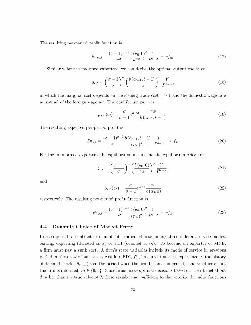
The resulting per-period profit function is

Eπm,t =(σ − 1)σ−1

σσb (a0, 0)σ

w∗σ−1

Y

P δ−σ− wfm, (17)

Similarly, for the informed exporters, we can derive the optimal output choice as

qx,t =

(σ − 1

σ

)σ (b (at−1, t− 1)

τw

)σ Y

P δ−σ, (18)

in which the marginal cost depends on the iceberg trade cost τ > 1 and the domestic wage rate

w instead of the foreign wage w∗. The equilibrium price is

px,t (at) =σ

σ − 1eat/σ

τw

b (at−1, t− 1). (19)

The resulting expected per-period profit is

Eπx,t =(σ − 1)σ−1

σσb (at−1, t− 1)σ

(τw)σ−1

Y

P δ−σ− wfx. (20)

For the uninformed exporters, the equilibrium output and the equilibrium price are

qx,t =

(σ − 1

σ

)σ (b (a0, 0)

τw

)σ Y

P δ−σ, (21)

and

px,t (at) =σ

σ − 1eat/σ

τw

b (a0, 0)(22)

respectively. The resulting per-period profit function is

Eπx,t =(σ − 1)σ−1

σσb (a0, 0)σ

(τw)σ−1

Y

P δ−σ− wfx. (23)

4.4 Dynamic Choice of Market Entry

In each period, an entrant or incumbent firm can choose among three different service modes:

exiting, exporting (denoted as x) or FDI (denoted as m). To become an exporter or MNE,

a firm must pay a sunk cost. A firm’s state variables include its mode of service in previous

period, o, the draw of sunk entry cost into FDI, fem, its current market experience, t, the history

of demand shocks, at−1 (from the period when the firm becomes informed), and whether or not

the firm is informed, in ∈ {0, 1}. Since firms make optimal decisions based on their belief about

θ rather than the true value of θ, these variables are sufficient to characterize the value functions

30

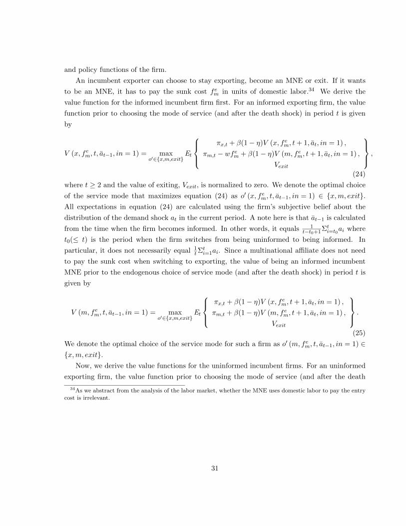
and policy functions of the firm.

An incumbent exporter can choose to stay exporting, become an MNE or exit. If it wants

to be an MNE, it has to pay the sunk cost fem in units of domestic labor.34 We derive the

value function for the informed incumbent firm first. For an informed exporting firm, the value

function prior to choosing the mode of service (and after the death shock) in period t is given

by

V (x, fem, t, at−1, in = 1) = maxo′∈{x,m,exit}

Et

πx,t + β(1− η)V (x, fem, t+ 1, at, in = 1) ,

πm,t − wfem + β(1− η)V (m, fem, t+ 1, at, in = 1) ,

Vexit

,

(24)

where t ≥ 2 and the value of exiting, Vexit, is normalized to zero. We denote the optimal choice

of the service mode that maximizes equation (24) as o′ (x, fem, t, at−1, in = 1) ∈ {x,m, exit}.All expectations in equation (24) are calculated using the firm’s subjective belief about the

distribution of the demand shock at in the current period. A note here is that at−1 is calculated

from the time when the firm becomes informed. In other words, it equals 1t−t0+1Σt

i=t0ai where

t0(≤ t) is the period when the firm switches from being uninformed to being informed. In

particular, it does not necessarily equal 1tΣ

ti=1ai. Since a multinational affiliate does not need

to pay the sunk cost when switching to exporting, the value of being an informed incumbent

MNE prior to the endogenous choice of service mode (and after the death shock) in period t is

given by

V (m, fem, t, at−1, in = 1) = maxo′∈{x,m,exit}

Et

πx,t + β(1− η)V (x, fem, t+ 1, at, in = 1) ,

πm,t + β(1− η)V (m, fem, t+ 1, at, in = 1) ,

Vexit

.

(25)

We denote the optimal choice of the service mode for such a firm as o′ (m, fem, t, at−1, in = 1) ∈{x,m, exit}.

Now, we derive the value functions for the uninformed incumbent firms. For an uninformed

exporting firm, the value function prior to choosing the mode of service (and after the death

34As we abstract from the analysis of the labor market, whether the MNE uses domestic labor to pay the entrycost is irrelevant.

31

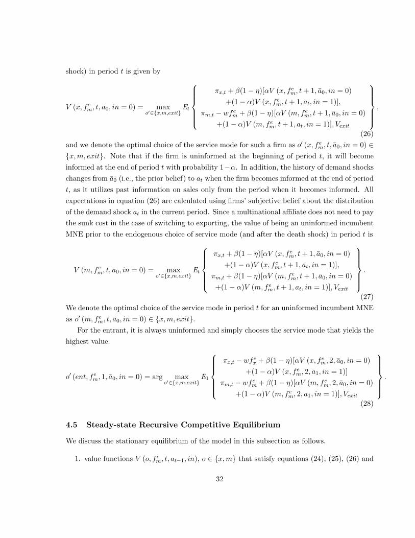
shock) in period t is given by

V (x, fem, t, a0, in = 0) = maxo′∈{x,m,exit}

Et

πx,t + β(1− η)[αV (x, fem, t+ 1, a0, in = 0)

+(1− α)V (x, fem, t+ 1, at, in = 1)],

πm,t − wfem + β(1− η)[αV (m, fem, t+ 1, a0, in = 0)

+(1− α)V (m, fem, t+ 1, at, in = 1)], Vexit

,

(26)

and we denote the optimal choice of the service mode for such a firm as o′ (x, fem, t, a0, in = 0) ∈{x,m, exit}. Note that if the firm is uninformed at the beginning of period t, it will become

informed at the end of period t with probability 1−α. In addition, the history of demand shocks

changes from a0 (i.e., the prior belief) to at when the firm becomes informed at the end of period

t, as it utilizes past information on sales only from the period when it becomes informed. All

expectations in equation (26) are calculated using firms’ subjective belief about the distribution

of the demand shock at in the current period. Since a multinational affiliate does not need to pay

the sunk cost in the case of switching to exporting, the value of being an uninformed incumbent

MNE prior to the endogenous choice of service mode (and after the death shock) in period t is

V (m, fem, t, a0, in = 0) = maxo′∈{x,m,exit}

Et

πx,t + β(1− η)[αV (x, fem, t+ 1, a0, in = 0)

+(1− α)V (x, fem, t+ 1, at, in = 1)],

πm,t + β(1− η)[αV (m, fem, t+ 1, a0, in = 0)

+(1− α)V (m, fem, t+ 1, at, in = 1)], Vexit

.

(27)

We denote the optimal choice of the service mode in period t for an uninformed incumbent MNE

as o′ (m, fem, t, a0, in = 0) ∈ {x,m, exit}.For the entrant, it is always uninformed and simply chooses the service mode that yields the

highest value:

o′ (ent, fem, 1, a0, in = 0) = arg maxo′∈{x,m,exit}

E1

πx,t − wfex + β(1− η)[αV (x, fem, 2, a0, in = 0)

+(1− α)V (x, fem, 2, a1, in = 1)]

πm,t − wfem + β(1− η)[αV (m, fem, 2, a0, in = 0)

+(1− α)V (m, fem, 2, a1, in = 1)], Vexit

.

(28)

4.5 Steady-state Recursive Competitive Equilibrium

We discuss the stationary equilibrium of the model in this subsection as follows.

1. value functions V (o, fem, t, at−1, in), o ∈ {x,m} that satisfy equations (24), (25), (26) and

32

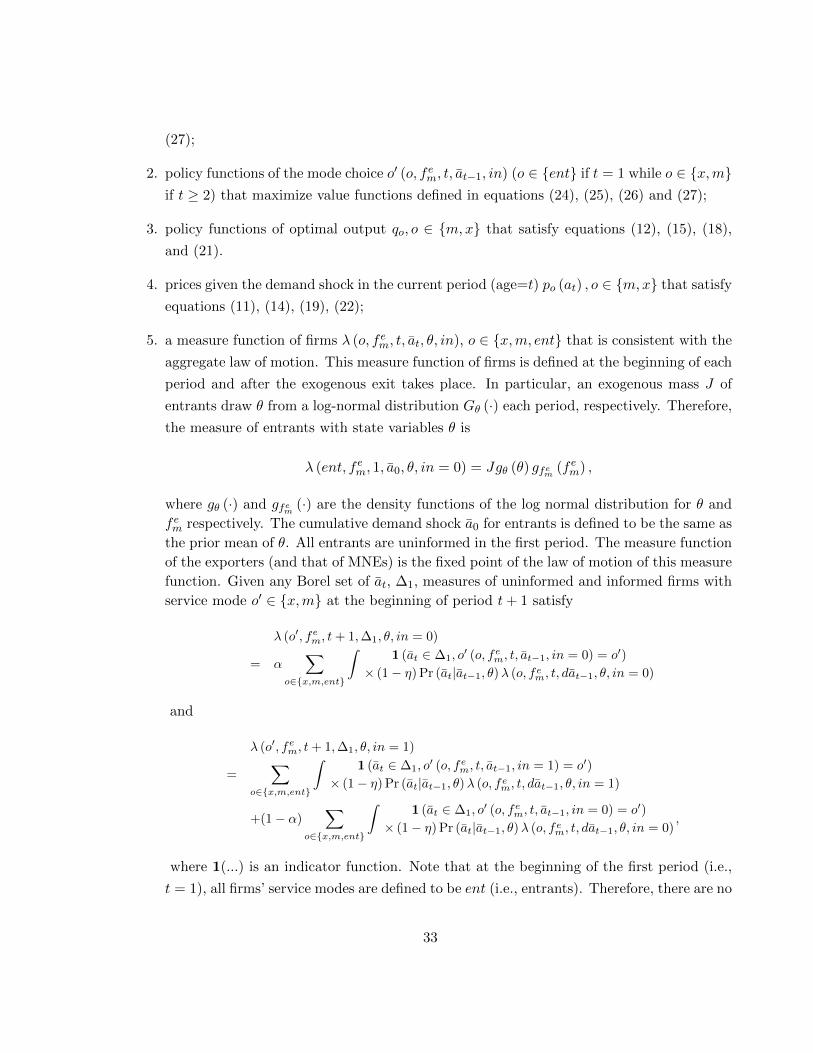
(27);

2. policy functions of the mode choice o′ (o, fem, t, at−1, in) (o ∈ {ent} if t = 1 while o ∈ {x,m}if t ≥ 2) that maximize value functions defined in equations (24), (25), (26) and (27);

3. policy functions of optimal output qo, o ∈ {m,x} that satisfy equations (12), (15), (18),

and (21).

4. prices given the demand shock in the current period (age=t) po (at) , o ∈ {m,x} that satisfy

equations (11), (14), (19), (22);

5. a measure function of firms λ (o, fem, t, at, θ, in), o ∈ {x,m, ent} that is consistent with the

aggregate law of motion. This measure function of firms is defined at the beginning of each

period and after the exogenous exit takes place. In particular, an exogenous mass J of

entrants draw θ from a log-normal distribution Gθ (·) each period, respectively. Therefore,

the measure of entrants with state variables θ is

λ (ent, fem, 1, a0, θ, in = 0) = Jgθ (θ) gfem (fem) ,

where gθ (·) and gfem (·) are the density functions of the log normal distribution for θ and

fem respectively. The cumulative demand shock a0 for entrants is defined to be the same as

the prior mean of θ. All entrants are uninformed in the first period. The measure function

of the exporters (and that of MNEs) is the fixed point of the law of motion of this measure

function. Given any Borel set of at, ∆1, measures of uninformed and informed firms with

service mode o′ ∈ {x,m} at the beginning of period t+ 1 satisfy

λ (o′, fem, t+ 1,∆1, θ, in = 0)

= α∑

o∈{x,m,ent}

∫1 (at ∈ ∆1, o

′ (o, fem, t, at−1, in = 0) = o′)

× (1− η) Pr (at|at−1, θ)λ (o, fem, t, dat−1, θ, in = 0)

and

λ (o′, fem, t+ 1,∆1, θ, in = 1)

=∑

o∈{x,m,ent}

∫1 (at ∈ ∆1, o

′ (o, fem, t, at−1, in = 1) = o′)

× (1− η) Pr (at|at−1, θ)λ (o, fem, t, dat−1, θ, in = 1)

+(1− α)∑

o∈{x,m,ent}

∫1 (at ∈ ∆1, o

′ (o, fem, t, at−1, in = 0) = o′)

× (1− η) Pr (at|at−1, θ)λ (o, fem, t, dat−1, θ, in = 0),

where 1(...) is an indicator function. Note that at the beginning of the first period (i.e.,

t = 1), all firms’ service modes are defined to be ent (i.e., entrants). Therefore, there are no

33

exporters or MNEs at age one in the stationary distribution, i.e., λ (o, fem, 1, a0, θ, in) = 0

for o ∈ {x,m}. In contrast, at the beginning of each later period (t ≥ 2), all incumbents’

modes of service are either exporting or FDI (i.e., x or m). Thus, there are no entrants at

t ≥ 2, i.e., λ (o, fem, t, at−1, θ, in) = 0 for o = ent and t ≥ 2.

6. the price index P is constant over time and must be consistent with consumer optimization

(3):

P 1−σ =∑t≥1

∑in∈{0,1}

o∈{x,m,ent}

∫fem,at−1,θ,at

eatpo (at, qo (b (at−1, t− 1) , in))1−σ

×λ (o, dfem, t, dat−1, dθ, in) dPr (at|θ).

Given each guess of P , we can solve for the value functions and policy functions, as well as the

measure function for firms, λ. We iterate on the value of P until it converges in the simulation

nd calibration.

4.6 Calibration and Counterfactual Analysis

In this section, we describe the procedures for calibrating the dynamic model proposed above.

The calibrated model is able to capture the decline in absolute value of FEs over affiliates’ life

cycle, as well as the smaller absolute value of FEs for affiliates with previous export experience.

It is also able to capture other salient features of the data, such as growth in exporters’ sales and

the decline in exit rates over their life cycles, which we do not directly target in the calibration.

After calibrating the model, we consider two counterfactual experiments with respect to the

variance of the fundamental demand draw and with respect to the variance of the transitory

demand shock.

4.6.1 Calibration

We first normalize a set of model primitives which are not identified since our model is not a

general equilibrium model. We normalize the exogenous aggregate demand shifter Y , the wage

rate in Japan, w, and the wage rate in the foreign countries, w∗ to one. The mean of the log of

the fundamental demand draw, µθ, is normalized to zero. We also normalize the entry costs into

exporting, fex, to zero, as we abstract from Japanese domestic firms in the model. Specifically,

moments that can be used to pin down fex, such as the share of exporters relative to domestic

firms, are not available. In this case, we should interpret the entry costs into FDI, fem, as the

entry costs into FDI relative to exporting.

Next, we calibrate a set of parameters without solving our model, as listed in Table 10. We

set the elasticity of substitution between varieties, σ, to 4, a common value in the literature (see

34

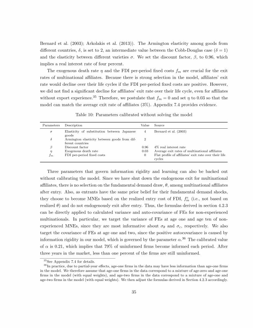
Bernard et al. (2003); Arkolakis et al. (2013)). The Armington elasticity among goods from

different countries, δ, is set to 2, an intermediate value between the Cobb-Douglas case (δ = 1)

and the elasticity between different varieties σ. We set the discount factor, β, to 0.96, which

implies a real interest rate of four percent.

The exogenous death rate η and the FDI per-period fixed costs fm are crucial for the exit

rates of multinational affiliates. Because there is strong selection in the model, affiliates’ exit

rate would decline over their life cycles if the FDI per-period fixed costs are positive. However,

we did not find a significant decline for affiliates’ exit rate over their life cycle, even for affiliates

without export experience.35 Therefore, we postulate that fm = 0 and set η to 0.03 so that the

model can match the average exit rate of affiliates (3%). Appendix 7.4 provides evidence.

Table 10: Parameters calibrated without solving the model

Parameters Description Value Source

σ Elasticity of substitution between Japanesegoods

4 Bernard et al. (2003)

δ Armington elasticity between goods from dif-ferent countries

2

β Discount factor 0.96 4% real interest rateη Exogenous death rate 0.03 Average exit rates of multinational affiliatesfm FDI per-period fixed costs 0 Flat profile of affiliates’ exit rate over their life

cycles

Three parameters that govern information rigidity and learning can also be backed out

without calibrating the model. Since we have shut down the endogenous exit for multinational

affiliates, there is no selection on the fundamental demand draw, θ, among multinational affiliates

after entry. Also, as entrants have the same prior belief for their fundamental demand shocks,

they choose to become MNEs based on the realized entry cost of FDI, fem (i.e., not based on

realized θ) and do not endogenously exit after entry. Thus, the formulas derived in section 4.2.3

can be directly applied to calculated variance and auto-covariance of FEs for non-experienced

multinationals. In particular, we target the variance of FEs at age one and age ten of non-

experienced MNEs, since they are most informative about σθ and σε, respectively. We also

target the covariance of FEs at age one and two, since the positive autocovariance is caused by

information rigidity in our model, which is governed by the parameter α.36 The calibrated value

of α is 0.21, which implies that 79% of uninformed firms become informed each period. After

three years in the market, less than one percent of the firms are still uninformed.

35See Appendix 7.4 for details.36In practice, due to partial-year effects, age-one firms in the data may have less information than age-one firms

in the model. We therefore assume that age-one firms in the data correspond to a mixture of age-zero and age-onefirms in the model (with equal weights), and age-two firms in the data correspond to a mixture of age-one andage-two firms in the model (with equal weights). We then adjust the formulas derived in Section 4.2.3 accordingly.

35

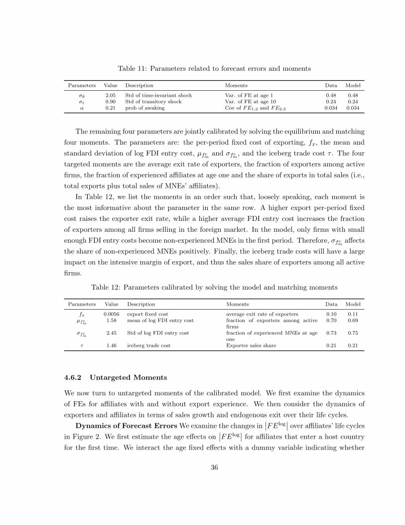
Table 11: Parameters related to forecast errors and moments

Parameters Value Description Moments Data Model

σθ 2.05 Std of time-invariant shock Var. of FE at age 1 0.48 0.48σε 0.90 Std of transitory shock Var. of FE at age 10 0.24 0.24α 0.21 prob of awaking Cov of FE1,2 and FE2,3 0.034 0.034

The remaining four parameters are jointly calibrated by solving the equilibrium and matching

four moments. The parameters are: the per-period fixed cost of exporting, fx, the mean and

standard deviation of log FDI entry cost, µfem and σfem , and the iceberg trade cost τ . The four

targeted moments are the average exit rate of exporters, the fraction of exporters among active

firms, the fraction of experienced affiliates at age one and the share of exports in total sales (i.e.,

total exports plus total sales of MNEs’ affiliates).

In Table 12, we list the moments in an order such that, loosely speaking, each moment is

the most informative about the parameter in the same row. A higher export per-period fixed

cost raises the exporter exit rate, while a higher average FDI entry cost increases the fraction

of exporters among all firms selling in the foreign market. In the model, only firms with small

enough FDI entry costs become non-experienced MNEs in the first period. Therefore, σfem affects

the share of non-experienced MNEs positively. Finally, the iceberg trade costs will have a large

impact on the intensive margin of export, and thus the sales share of exporters among all active

firms.

Table 12: Parameters calibrated by solving the model and matching moments

Parameters Value Description Moments Data Model

fx 0.0056 export fixed cost average exit rate of exporters 0.10 0.11µfem 1.58 mean of log FDI entry cost fraction of exporters among active

firms0.70 0.69

σfem 2.45 Std of log FDI entry cost fraction of experienced MNEs at ageone

0.73 0.75

τ 1.46 iceberg trade cost Exporter sales share 0.21 0.21

4.6.2 Untargeted Moments

We now turn to untargeted moments of the calibrated model. We first examine the dynamics

of FEs for affiliates with and without export experience. We then consider the dynamics of

exporters and affiliates in terms of sales growth and endogenous exit over their life cycles.

Dynamics of Forecast Errors We examine the changes in∣∣FElog

∣∣ over affiliates’ life cycles

in Figure 2. We first estimate the age effects on∣∣FElog

∣∣ for affiliates that enter a host country

for the first time. We interact the age fixed effects with a dummy variable indicating whether

36

the parent firm has previous export experience in the same region. We plot the estimated fixed

effects for experienced and non-experienced MNEs in the left panel of Figure 2, using the age-one

non-experienced MNEs as the base group. In the right panel, we plot the average∣∣FElog

∣∣ by

affiliate age predicted by the calibrated model, again normalizing the average∣∣FElog

∣∣ to zero

for non-experienced MNEs at age one.

Consistent with the data, the model predicts that average |FElog| declines over affiliates’

life cycles and that the initial∣∣FElog

∣∣ is lower for affiliates whose parent firms have export

experience. However, the model predicts a much smaller decline in∣∣FElog

∣∣ for experienced

MNEs and a larger difference between experienced MNEs and non-experienced MNEs at age

one. For example, in the model, average∣∣FElog

∣∣ of experienced MNEs drops by 0.02 over

their life cycles, while the corresponding empirical moment is 0.16. The main reason for this

discrepancy is that firms in the model learn very fast - there is almost no uncertainty about θ

after four periods. This implies experienced firms will start with very precise forecast about θ

and the main source of FEs is the transitory transitory shock, ε. A possible improvement we can

make is to introduce learning about both demand and supply and assume that exporting only

helps the firm learn foreign demand. This modification would reduce the information generated

by exporting (relative to MP). However, we do not pursue here in order to keep our model

simple.

Dynamics of Sales In Figure 3, we compare the age profile of exports in the model to that

in the data. The red dashed line represents the average log of sales by exporter age predicted by

the model, while the blue solid line represents the corresponding moments in the data. The two

lines are very well aligned. Note that learning and information rigidity per se do not generate

growth in sales, since firms may receive either better or worse signals than their time-invariant

demand. The growth of average firm size is a result of learning together with selection on θ

in the model. In contrast, the model does not capture the growth of average log sales of the

multinational affiliates. The reason is that we shut down endogenous exits of affiliates to match

the flat profile of exit rate (with firm age) over their life cycles. Other mechanisms, such as the

accumulation of customer capital, is needed to match the dynamics of sales for multinational

affiliates (see, for example, Fitzgerald et al. (2016)).

Dynamics of Exits Figure 4 compares the exporter exit rates by their ages in the model

to those in the data. Consistent with the data, the model predicts a declining trend in the

exit rates of exporters when they become older. In the model, the exporter exit rates decline

from 47% to 3% over their life cycles, while the exporter exit rates decline from 16% to 4%

in the data. Overall, the model predicts higher exporter exit rates (by each age group), even

though the model is able to match the average exporter exit rate in the data. This occurs as

37

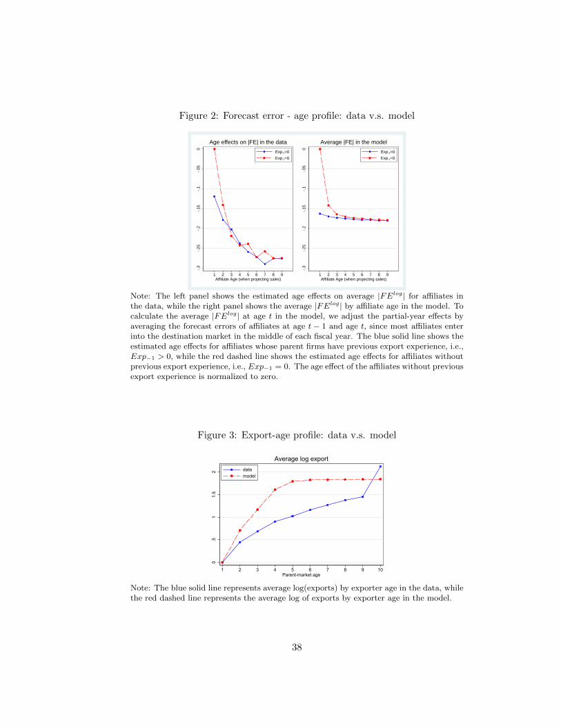
Figure 2: Forecast error - age profile: data v.s. model

-.3

-.25

-.2

-.15

-.1

-.05

0

1 2 3 4 5 6 7 8 9Affiliate Age (when projecting sales)

Exp-1>0

Exp-1=0

Age effects on |FE| in the data

-.3

-.25

-.2

-.15

-.1

-.05

0

1 2 3 4 5 6 7 8 9Affiliate Age (when projecting sales)

Exp-1>0

Exp-1=0

Average |FE| in the model

Note: The left panel shows the estimated age effects on average |FElog| for affiliates inthe data, while the right panel shows the average |FElog| by affiliate age in the model. Tocalculate the average |FElog| at age t in the model, we adjust the partial-year effects byaveraging the forecast errors of affiliates at age t − 1 and age t, since most affiliates enterinto the destination market in the middle of each fiscal year. The blue solid line shows theestimated age effects for affiliates whose parent firms have previous export experience, i.e.,Exp−1 > 0, while the red dashed line shows the estimated age effects for affiliates withoutprevious export experience, i.e., Exp−1 = 0. The age effect of the affiliates without previousexport experience is normalized to zero.

Figure 3: Export-age profile: data v.s. model

0.5

11.

52

1 2 3 4 5 6 7 8 9 10Parent-market age

datamodel

Average log export

Note: The blue solid line represents average log(exports) by exporter age in the data, whilethe red dashed line represents the average log of exports by exporter age in the model.

38

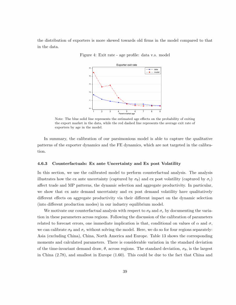
the distribution of exporters is more skewed towards old firms in the model compared to that

in the data.

Figure 4: Exit rate - age profile: data v.s. model

0.1

.2.3

.4.5

1 2 3 4 5 6 7 8 9Parent-market age

datamodel

Exporter exit rate

Note: The blue solid line represents the estimated age effects on the probability of exitingthe export market in the data, while the red dashed line represents the average exit rate ofexporters by age in the model.

In summary, the calibration of our parsimonious model is able to capture the qualitative

patterns of the exporter dynamics and the FE dynamics, which are not targeted in the calibra-

tion.

4.6.3 Counterfactuals: Ex ante Uncertainty and Ex post Volatility

In this section, we use the calibrated model to perform counterfactual analysis. The analysis

illustrates how the ex ante uncertainty (captured by σθ) and ex post volatility (captured by σε)

affect trade and MP patterns, the dynamic selection and aggregate productivity. In particular,

we show that ex ante demand uncertainty and ex post demand volatility have qualitatively

different effects on aggregate productivity via their different impact on the dynamic selection

(into different production modes) in our industry equilibrium model.

We motivate our counterfactual analysis with respect to σθ and σε by documenting the varia-

tion in these parameters across regions. Following the discussion of the calibration of parameters

related to forecast errors, one immediate implication is that, conditional on values of α and σ,

we can calibrate σθ and σε without solving the model. Here, we do so for four regions separately:

Asia (excluding China), China, North America and Europe. Table 13 shows the corresponding

moments and calculated parameters. There is considerable variation in the standard deviation

of the time-invariant demand draw, θ, across regions. The standard deviation, σθ, is the largest

in China (2.78), and smallest in Europe (1.60). This could be due to the fact that China and

39

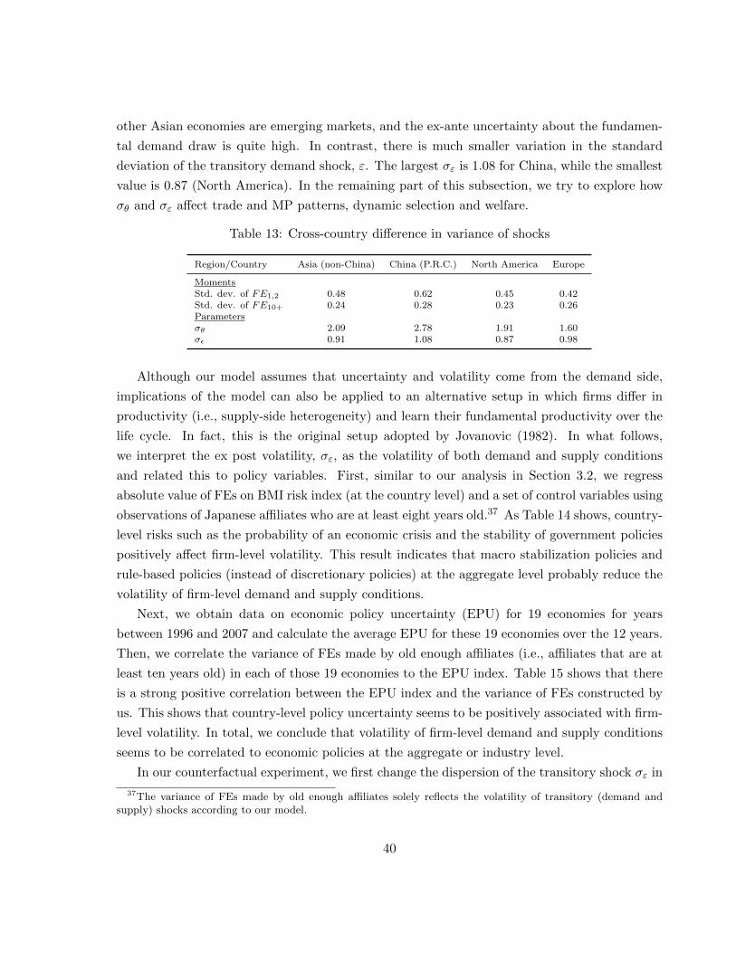
other Asian economies are emerging markets, and the ex-ante uncertainty about the fundamen-

tal demand draw is quite high. In contrast, there is much smaller variation in the standard

deviation of the transitory demand shock, ε. The largest σε is 1.08 for China, while the smallest

value is 0.87 (North America). In the remaining part of this subsection, we try to explore how

σθ and σε affect trade and MP patterns, dynamic selection and welfare.

Table 13: Cross-country difference in variance of shocks

Region/Country Asia (non-China) China (P.R.C.) North America Europe

MomentsStd. dev. of FE1,2 0.48 0.62 0.45 0.42Std. dev. of FE10+ 0.24 0.28 0.23 0.26Parametersσθ 2.09 2.78 1.91 1.60σε 0.91 1.08 0.87 0.98

Although our model assumes that uncertainty and volatility come from the demand side,

implications of the model can also be applied to an alternative setup in which firms differ in

productivity (i.e., supply-side heterogeneity) and learn their fundamental productivity over the

life cycle. In fact, this is the original setup adopted by Jovanovic (1982). In what follows,

we interpret the ex post volatility, σε, as the volatility of both demand and supply conditions

and related this to policy variables. First, similar to our analysis in Section 3.2, we regress

absolute value of FEs on BMI risk index (at the country level) and a set of control variables using

observations of Japanese affiliates who are at least eight years old.37 As Table 14 shows, country-

level risks such as the probability of an economic crisis and the stability of government policies

positively affect firm-level volatility. This result indicates that macro stabilization policies and

rule-based policies (instead of discretionary policies) at the aggregate level probably reduce the

volatility of firm-level demand and supply conditions.

Next, we obtain data on economic policy uncertainty (EPU) for 19 economies for years

between 1996 and 2007 and calculate the average EPU for these 19 economies over the 12 years.

Then, we correlate the variance of FEs made by old enough affiliates (i.e., affiliates that are at

least ten years old) in each of those 19 economies to the EPU index. Table 15 shows that there

is a strong positive correlation between the EPU index and the variance of FEs constructed by

us. This shows that country-level policy uncertainty seems to be positively associated with firm-

level volatility. In total, we conclude that volatility of firm-level demand and supply conditions

seems to be correlated to economic policies at the aggregate or industry level.

In our counterfactual experiment, we first change the dispersion of the transitory shock σε in

37The variance of FEs made by old enough affiliates solely reflects the volatility of transitory (demand andsupply) shocks according to our model.

40

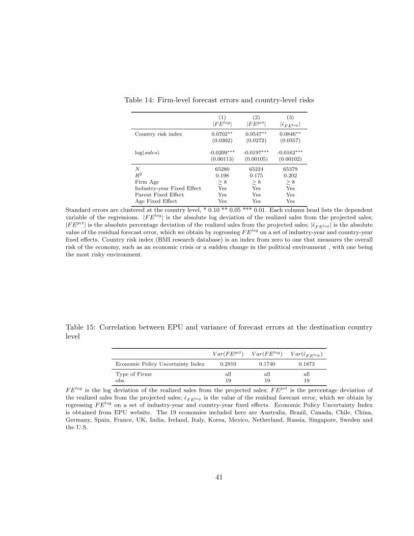
Table 14: Firm-level forecast errors and country-level risks

(1) (2) (3)|FElog | |FEpct| |εFElog |

Country risk index 0.0702∗∗ 0.0547∗∗ 0.0846∗∗

(0.0302) (0.0272) (0.0357)

log(sales) -0.0209∗∗∗ -0.0197∗∗∗ -0.0162∗∗∗

(0.00113) (0.00105) (0.00102)

N 65280 65224 65379R2 0.198 0.175 0.202Firm Age ≥ 8 ≥ 8 ≥ 8Industry-year Fixed Effect Yes Yes YesParent Fixed Effect Yes Yes YesAge Fixed Effect Yes Yes Yes

Standard errors are clustered at the country level, * 0.10 ** 0.05 *** 0.01. Each column head lists the dependentvariable of the regressions. |FElog| is the absolute log deviation of the realized sales from the projected sales;|FEpct| is the absolute percentage deviation of the realized sales from the projected sales; |εFElog | is the absolutevalue of the residual forecast error, which we obtain by regressing FElog on a set of industry-year and country-yearfixed effects. Country risk index (BMI research database) is an index from zero to one that measures the overallrisk of the economy, such as an economic crisis or a sudden change in the political environment , with one beingthe most risky environment.

Table 15: Correlation between EPU and variance of forecast errors at the destination countrylevel

V ar(FEpct) V ar(FElog) V ar(εFElog )

Economic Policy Uncertainty Index 0.2910 0.1740 0.1873

Type of Firms all all allobs. 19 19 19

FElog is the log deviation of the realized sales from the projected sales; FEpct is the percentage deviation ofthe realized sales from the projected sales; εFElog is the value of the residual forecast error, which we obtain byregressing FElog on a set of industry-year and country-year fixed effects. Economic Policy Uncertainty Indexis obtained from EPU website. The 19 economies included here are Australia, Brazil, Canada, Chile, China,Germany, Spain, France, UK, India, Ireland, Italy, Korea, Mexico, Netherland, Russia, Singapore, Sweden andthe U.S.

41

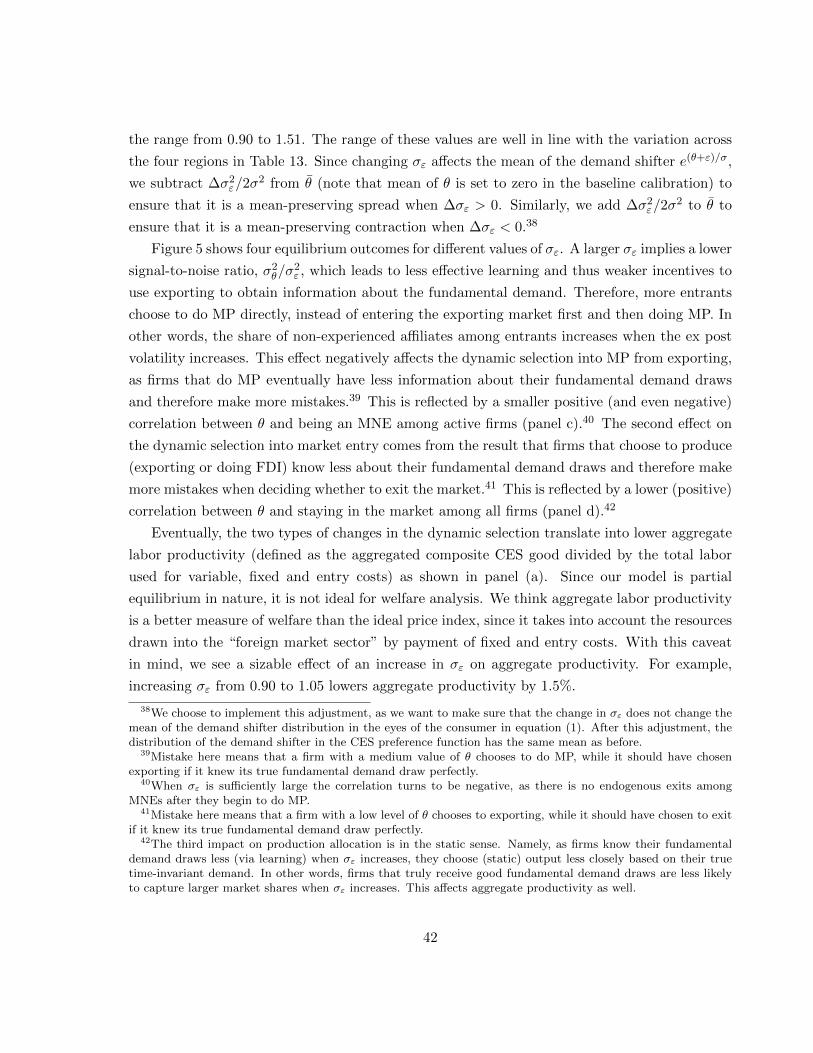
the range from 0.90 to 1.51. The range of these values are well in line with the variation across

the four regions in Table 13. Since changing σε affects the mean of the demand shifter e(θ+ε)/σ,

we subtract ∆σ2ε/2σ

2 from θ (note that mean of θ is set to zero in the baseline calibration) to

ensure that it is a mean-preserving spread when ∆σε > 0. Similarly, we add ∆σ2ε/2σ

2 to θ to

ensure that it is a mean-preserving contraction when ∆σε < 0.38

Figure 5 shows four equilibrium outcomes for different values of σε. A larger σε implies a lower

signal-to-noise ratio, σ2θ/σ

2ε , which leads to less effective learning and thus weaker incentives to

use exporting to obtain information about the fundamental demand. Therefore, more entrants

choose to do MP directly, instead of entering the exporting market first and then doing MP. In

other words, the share of non-experienced affiliates among entrants increases when the ex post

volatility increases. This effect negatively affects the dynamic selection into MP from exporting,

as firms that do MP eventually have less information about their fundamental demand draws

and therefore make more mistakes.39 This is reflected by a smaller positive (and even negative)

correlation between θ and being an MNE among active firms (panel c).40 The second effect on

the dynamic selection into market entry comes from the result that firms that choose to produce

(exporting or doing FDI) know less about their fundamental demand draws and therefore make

more mistakes when deciding whether to exit the market.41 This is reflected by a lower (positive)

correlation between θ and staying in the market among all firms (panel d).42

Eventually, the two types of changes in the dynamic selection translate into lower aggregate

labor productivity (defined as the aggregated composite CES good divided by the total labor

used for variable, fixed and entry costs) as shown in panel (a). Since our model is partial

equilibrium in nature, it is not ideal for welfare analysis. We think aggregate labor productivity

is a better measure of welfare than the ideal price index, since it takes into account the resources

drawn into the “foreign market sector” by payment of fixed and entry costs. With this caveat

in mind, we see a sizable effect of an increase in σε on aggregate productivity. For example,

increasing σε from 0.90 to 1.05 lowers aggregate productivity by 1.5%.

38We choose to implement this adjustment, as we want to make sure that the change in σε does not change themean of the demand shifter distribution in the eyes of the consumer in equation (1). After this adjustment, thedistribution of the demand shifter in the CES preference function has the same mean as before.

39Mistake here means that a firm with a medium value of θ chooses to do MP, while it should have chosenexporting if it knew its true fundamental demand draw perfectly.

40When σε is sufficiently large the correlation turns to be negative, as there is no endogenous exits amongMNEs after they begin to do MP.

41Mistake here means that a firm with a low level of θ chooses to exporting, while it should have chosen to exitif it knew its true fundamental demand draw perfectly.

42The third impact on production allocation is in the static sense. Namely, as firms know their fundamentaldemand draws less (via learning) when σε increases, they choose (static) output less closely based on their truetime-invariant demand. In other words, firms that truly receive good fundamental demand draws are less likelyto capture larger market shares when σε increases. This affects aggregate productivity as well.

42

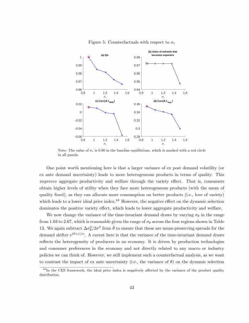
Figure 5: Counterfactuals with respect to σε

0.8 1 1.2 1.4 1.60.96

0.97

0.98

0.99

1(a) Q/L

0.8 1 1.2 1.4 1.60.94

0.95

0.96

0.97

0.98

(b) share of entrants thatbecomes exporters

0.8 1 1.2 1.4 1.6-0.06

-0.04

-0.02

0

0.02(c) Corr( ,1MNE)

0.8 1 1.2 1.4 1.60.28

0.3

0.32

0.34

0.36(d) Corr( ,1stay )

Note: The value of σε is 0.90 in the baseline equilibrium, which is marked with a red circlein all panels.

One point worth mentioning here is that a larger variance of ex post demand volatility (or

ex ante demand uncertainty) leads to more heterogeneous products in terms of quality. This

improves aggregate productivity and welfare through the variety effect. That is, consumers

obtain higher levels of utility when they face more heterogeneous products (with the mean of

quality fixed), as they can allocate more consumption on better products (i.e., love of variety)

which leads to a lower ideal price index.43 However, the negative effect on the dynamic selection

dominates the positive variety effect, which leads to lower aggregate productivity and welfare.

We now change the variance of the time-invariant demand draws by varying σθ in the range

from 1.03 to 2.67, which is reasonable given the range of σθ across the four regions shown in Table

13. We again subtract ∆σ2θ/2σ

2 from θ to ensure that these are mean-preserving spreads for the

demand shifter e(θ+ε)/σ. A caveat here is that the variance of the time-invariant demand draws

reflects the heterogeneity of producers in an economy. It is driven by production technologies

and consumer preferences in the economy and not directly related to any macro or industry

policies we can think of. However, we still implement such a counterfactual analysis, as we want

to contrast the impact of ex ante uncertainty (i.e., the variance of θ) on the dynamic selection

43In the CES framework, the ideal price index is negatively affected by the variance of the product qualitydistribution.

43

with the effect of ex post volatility (i.e., the variance of ε).

Broadly speaking, the effect of an increase in ex ante uncertainty on the dynamic selection

is exactly the opposite to the effect of an increase in ex post volatility, as it implies a higher

signal-to-noise ratio and therefore increases the effectiveness of learning. In short, the dynamic

selection is positively affected by such an increase, as both the (positive) correlation between

θ and being a multinational firm among active firms (panel c) and the (positive) correlation

between θ and staying in the market (panel d) increase with the variance of the time-invariant

demand draws. Eventually, these effects translate into higher aggregate productivity when the

variance of ex ante uncertainty increases, which is the opposite to the effect of an increase in ex

post volatility.

Figure 6: Counterfactuals with respect to σθ

1 1.5 2 2.5 30.5

1

1.5

2(a) Q/L

1 1.5 2 2.5 30.9

0.95

1

(b) share of entrants thatbecomes exporters

1 1.5 2 2.5 3-0.1

0

0.1

0.2(c) Corr( ,1MNE)

1 1.5 2 2.5 30.2

0.3

0.4

0.5(d) Corr( ,1stay )

Note: The value of σθ is 2.05 in the baseline equilibrium, which is marked with a red circlein all panels.

In summary, both the uncertainty of ex ante fundamental demand (or productivity) draws

and the volatility of ex post transitory shocks contribute to firm-level uncertainty in our model.

However, the effects of these two types of uncertainty on dynamic trade/MP patterns, the

dynamic selection and aggregate productivity are different. Therefore, in order to understand the

effect of uncertainty on aggregate and dynamic economic outcomes, it is important to distinguish

between these two sources of uncertainty.

44

5 Conclusion

In this paper, we use a unique dataset of Japanese multinational affiliates, which contains infor-

mation on sales forecasts, to detect information imperfection and learning in the international

market. We document three stylized facts concerning affiliates’ forecasts. First, FEs of sales

decline with the age of affiliate. Second, if the parent firm has previous export experience to the

region where its affiliate is set up, the entering affiliate starts with a smaller variance of FEs.

Third, FEs of sales are positively correlated over time and this positive correlation becomes

stronger when the affiliates are located further away from Japan, which are inconsistent with

predictions from FIRE models. In total, We view these facts as direct evidence for the existence

of imperfect information and learning in the international market. We then build up a dynamic

industry equilibrium model of trade and FDI, which features information rigidity and learning,

in order to explain the documented facts.

To quantify the role of learning and demand uncertainty in exporters and multinational

firms’ dynamics, we extend the standard firm learning model (Jovanovic (1982); Arkolakis et

al. (2017)) into an international setting. Specifically, we add sticky information a la Mankiw

and Reis (2002) and the endogenous choice between exporting and MP (for serving the foreign

market) into the canonical firm learning model and calibrate the extended model to match

moments related to FEs and aggregate trade/MP variables. The calibrated model is able to

replicate the new facts about affiliates’ FEs, as well as other salient features of the data.

We then conduct counterfactual analysis regarding firm-level uncertainty. We find that

changing the variance of the time-invariant demand draws and that of the temporary demand

shocks have different implications for the entry margins of trade and MP, dynamic selection and

aggregate productivity. In particular, a higher variance of time-invariant demand draws implies

a higher signal-to-noise ratio. This leads to more effective learning and stronger incentives to

use exporting to obtain information. To the contrary, a higher variance of the transitory shocks

implies a lower signal-to-noise ratio and leads to less effective learning. As a result, dynamic

selection is negatively affected by ex post volatility, which leads to lower aggregate productivity

and welfare. In short, our exercises show that when we analyze how uncertainty affects aggregate

outcomes, it is crucial to distinguish between the two sources of uncertainty discussed above.

45

6 Theory Appendix

6.1 Full Information Rational Expectation Models

In this subsection, we derive the FE in FIRE models in detail. Base on the optimal output

choice derived in the main text we have the log of realized sales as

log(Rt(θ)) = log(At) +σθ + εt + (σ−1)σ2

ε2σ

σ+ (σ − 1)

[log(σ − 1

σw

)].

Since the firm knows θ in FIRE models, its best estimate for at is θ as εt is a transitory i.i.d.

shock. Therefore, the conditional distribution of at in any period is N(θ, σ2

ε

), and the log of

forecasted sales is

log(

ESt−1(Rt))

= log(At) +σθ + σ2

ε2

σ+ (σ − 1)

[log(σ − 1

σw

)],

which leads to

FElogt−1,t(sales) =

εtσ− σ2

ε

2σ2. (29)

Note that when the firm forecasts its sales one period in advance, it still faces an unpredictable

random shock (i,e., εt) which causes FEs even in the full information model. Note that as

the contemporaneous transitory shock in demand follows the log normal distribution, higher

variance of the transitory shock pushes up the forecasted sales, price and output.

6.2 Full Information Rational Expectation Models with Endogenous Exit

We discuss how the endogenous exit would change full information rational expectation (FIRE)

model’s prediction on the serial correlation of FEs. In order to generate endogenous exit, we

consider the case in which the fundamental demand, θ, evolves according to an AR(1) process:

θt+1 = ρ1θt + ζt+1, (30)

where ζt is a draw from a normal distribution N(

0, σ2ζ

)and serially uncorrelated. The resulting

FE and serial correlation of FEs are

FElogt−1,t(sales) =

εtσ− σ2

ε

2σ2+ζtσ−

σ2ζ

2σ2. (31)

and

cov(FElogt−1,t, FE

logt,t+1) = cov

(εt + ζtσ

,εt+1 + ζt+1

σ

)46

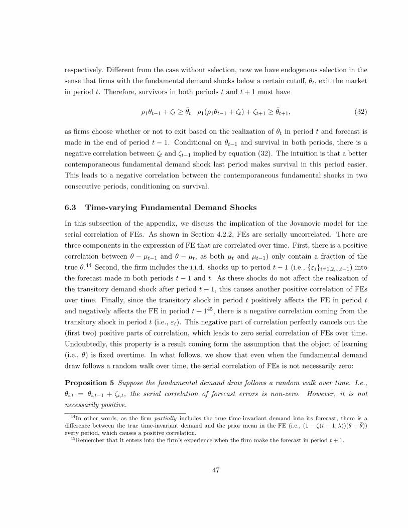
respectively. Different from the case without selection, now we have endogenous selection in the

sense that firms with the fundamental demand shocks below a certain cutoff, θt, exit the market

in period t. Therefore, survivors in both periods t and t+ 1 must have

ρ1θt−1 + ζt ≥ θt ρ1(ρ1θt−1 + ζt) + ζt+1 ≥ θt+1, (32)

as firms choose whether or not to exit based on the realization of θt in period t and forecast is

made in the end of period t − 1. Conditional on θt−1 and survival in both periods, there is a

negative correlation between ζt and ζt−1 implied by equation (32). The intuition is that a better

contemporaneous fundamental demand shock last period makes survival in this period easier.

This leads to a negative correlation between the contemporaneous fundamental shocks in two

consecutive periods, conditioning on survival.

6.3 Time-varying Fundamental Demand Shocks

In this subsection of the appendix, we discuss the implication of the Jovanovic model for the

serial correlation of FEs. As shown in Section 4.2.2, FEs are serially uncorrelated. There are

three components in the expression of FE that are correlated over time. First, there is a positive

correlation between θ − µt−1 and θ − µt, as both µt and µt−1) only contain a fraction of the

true θ.44 Second, the firm includes the i.i.d. shocks up to period t− 1 (i.e., {εi}i=1,2,...t−1) into

the forecast made in both periods t − 1 and t. As these shocks do not affect the realization of

the transitory demand shock after period t− 1, this causes another positive correlation of FEs

over time. Finally, since the transitory shock in period t positively affects the FE in period t

and negatively affects the FE in period t+ 145, there is a negative correlation coming from the

transitory shock in period t (i.e., εt). This negative part of correlation perfectly cancels out the

(first two) positive parts of correlation, which leads to zero serial correlation of FEs over time.

Undoubtedly, this property is a result coming form the assumption that the object of learning

(i.e., θ) is fixed overtime. In what follows, we show that even when the fundamental demand

draw follows a random walk over time, the serial correlation of FEs is not necessarily zero:

Proposition 5 Suppose the fundamental demand draw follows a random walk over time. I.e.,

θi,t = θi,t−1 + ζi,t, the serial correlation of forecast errors is non-zero. However, it is not

necessarily positive.

44In other words, as the firm partially includes the true time-invariant demand into its forecast, there is adifference between the true time-invariant demand and the prior mean in the FE (i.e., (1 − ζ(t − 1, λ))(θ − θ))every period, which causes a positive correlation.

45Remember that it enters into the firm’s experience when the firm make the forecast in period t+ 1.

47

Proof. We consider the following learning model:

θi,t = θi,t−1 + ζi,t

and

ai,t = θi,t + εi,t,

where ai,t is the realized overall demand shock which is observable, while θi,t is the time-variant

fundamental demand draw which is unobservable.

We solve the steady state first. Standard argument leads to the result that

Σss =σ2ζ +K2σ2

ε

1− (1−K)2

and

K =Σss

σ2ε + Σss

,

where Σss is the variance of filtering error of θi in the steady state, and K is the Kalman gain

(i.e., the weight put on the new signal when updating the belief) in the steady state. After

solving these two equations, we obtain

K(λ) =1

2(−λ+

√λ2 + 4λ), (33)

where λ ≡ σ2ζ

σ2ε

is the signal-noise ratio (i.e., the precision of the signal).

Next, we consider non-steady state forecasting. In order to forecast ai,t+1, the firm needs

to predict θi,t as Etai,t+1 = Etθi,t+1 = Etθi,t. The prediction for θi,t at the end of period t is

denoted by θi,t (i.e., filtering). Based on the timing assumption of our model, θi,0 = θ0 which

is the prior belief. Suppose firms start from different fundamental demand shocks but have the

same prior belief for θi,0: N(θ0,Σ0). As we are not in the steady state, the Kalman gains are

time-variant. In particular, the forecasting rule is as follows:

θt = (1−Kt)θt−1 +Ktat, (34)

48

FE of θi,t+1 in period t+ 1 is

et+1 = θt+1 − θt+1

= θt+1 − (1−Kt+1)θt −Kt+1 (θt+1 + εt+1)

= (1−Kt+1)(θt + ζt+1 − θt

)−Kt+1εt+1

= (1−Kt+1) (et + ζt+1)−Kt+1εt+1

The equation that governs the movement of variance of FEs is

Σt+1 = (1−Kt+1)2(Σt + σ2

ζ

)+K2

t+1σ2ε , (35)

where Σt = var(et), we start with Σ0 which is the ex ante variance of of θ0. Minimizing Σt+1

leads to the result that

Kt+1 =ρ2Σt + σ2

ζ

Σt + σ2ζ + σ2

ε

K ≥ 0. (36)

Now, we can calculate the serial correlation of FEs over the firm’s life cycle. The expression

for FElogt,t+1(sales) can be expressed as

θt+1 + εt+1 − θtσ

−Σt + σ2

ζ + σ2ε

2σ2,

Since ut is uncorrelated over time, the stochastic term that is correlated over time is

1

σ

[θt+1 + εt+1 −

[Kt(θt + εt) + (1−Kt)Kt−1(θt−1 + εt−1)

+...(1−Kt−1)(1−Kt−2)...(1−K2)[K1(θ1 + ε1) + (1−K1)θ0]]].

Since the above expression is hard to calculate in general, let us focus on age one firms and age

two firms first:

cov(FElog1,2 , FE

log2,3) =

1

σ2cov(

(ε2 −K1ε1) + (ζ2 + (1−K1)ζ1),

(ε3 −K2ε2 − (1−K2)K1ε1) + (ζ3 + (1−K2)ζ2 + (1−K2)(1−K1)ζ1)).

which equals

(1−K2)[σ2εK

21 + σ2

ζ (1 + (1−K1)2)]− σ2εK2,

which can be either positive or negative. In particular, if K2 (i.e., the Kalman gain in period

49

two) is close to one, the whole term becomes negative which is inconsistent with our empirical

finding.

6.4 Volatility of Output Growth

In this subsection of the appendix, we show that the Jovanovic model predicts that the volatility

of growth rate of output decreases with firm age, which is a salient feature of our data. The

learning model provides a rationale for this, even in the case in which the volatility of productivity

or demand shocks does not vary with age.

Proposition 6 Growth volatility of output decreases with firm age. Growth volatility of sales

decreases with firm age at least when the firm is young.

Proof. Based on equation (41), we know that log firm output at age t is proportional to (after

omitting constants and aggregate variables which are constant in the steady state)

σ log(b(a, t− 1)), (37)

and it is proportional to

σ log(b(a, t)), (38)

at age t+1. Therefore, the growth rate of output or quantity (or the log difference) is proportional

to46 (λ(θ − θ) + (1 + λ(t− 1))λεt − λ2Σt−1i=1εi

(1 + λt)(1 + λ(t− 1))

).

The variance of the growth rate at age t (t ≥ 2) is

var(growth rate)t =[ λ2σ2

θ + λ4σ2ε(t− 1)

(1 + λt)2(1 + λ(t− 1))2+( λ

(1 + λt)

)2σ2ε

],

which can be reduced to

var(growth rate)t =( λ2σ2

ε

(1 + λt)(1 + λ(t− 1))

).

Thus, the growth volatility of output decreases with firm age.

Next, we explore how the growth volatility of sales varies with firm age. Based on equation

(41), we know that log firm sales at age t are proportional to (after omitting constants and

46Here, we omit the term related to 12

(σ2t−1+σ2

ε

σ

)and 1

2

(σ2t +σ2

εσ

), as they do not vary across firms.

50

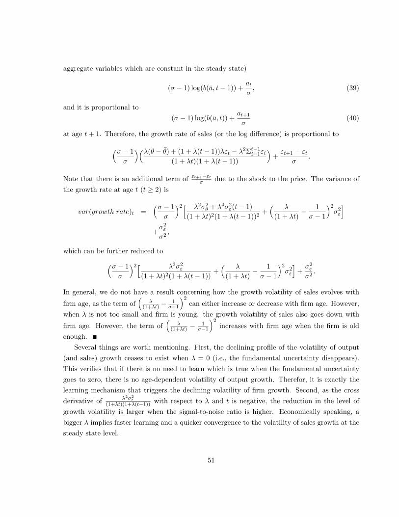
aggregate variables which are constant in the steady state)

(σ − 1) log(b(a, t− 1)) +atσ, (39)

and it is proportional to

(σ − 1) log(b(a, t)) +at+1

σ(40)

at age t+ 1. Therefore, the growth rate of sales (or the log difference) is proportional to

(σ − 1

σ

)(λ(θ − θ) + (1 + λ(t− 1))λεt − λ2Σt−1i=1εi

(1 + λt)(1 + λ(t− 1))

)+εt+1 − εt

σ.

Note that there is an additional term of εt+1−εtσ due to the shock to the price. The variance of

the growth rate at age t (t ≥ 2) is

var(growth rate)t =(σ − 1

σ

)2[ λ2σ2θ + λ4σ2

ε(t− 1)

(1 + λt)2(1 + λ(t− 1))2+( λ

(1 + λt)− 1

σ − 1

)2σ2ε

]+σ2ε

σ2,

which can be further reduced to(σ − 1

σ

)2[ λ3σ2ε

(1 + λt)2(1 + λ(t− 1))+( λ

(1 + λt)− 1

σ − 1

)2σ2ε

]+σ2ε

σ2.

In general, we do not have a result concerning how the growth volatility of sales evolves with

firm age, as the term of(

λ(1+λt) −

1σ−1

)2can either increase or decrease with firm age. However,

when λ is not too small and firm is young. the growth volatility of sales also goes down with

firm age. However, the term of(

λ(1+λt) −

1σ−1

)2increases with firm age when the firm is old

enough.

Several things are worth mentioning. First, the declining profile of the volatility of output

(and sales) growth ceases to exist when λ = 0 (i.e., the fundamental uncertainty disappears).

This verifies that if there is no need to learn which is true when the fundamental uncertainty

goes to zero, there is no age-dependent volatility of output growth. Therefor, it is exactly the

learning mechanism that triggers the declining volatility of firm growth. Second, as the cross

derivative of λ2σ2ε

(1+λt)(1+λ(t−1)) with respect to λ and t is negative, the reduction in the level of

growth volatility is larger when the signal-to-noise ratio is higher. Economically speaking, a

bigger λ implies faster learning and a quicker convergence to the volatility of sales growth at the

steady state level.

51

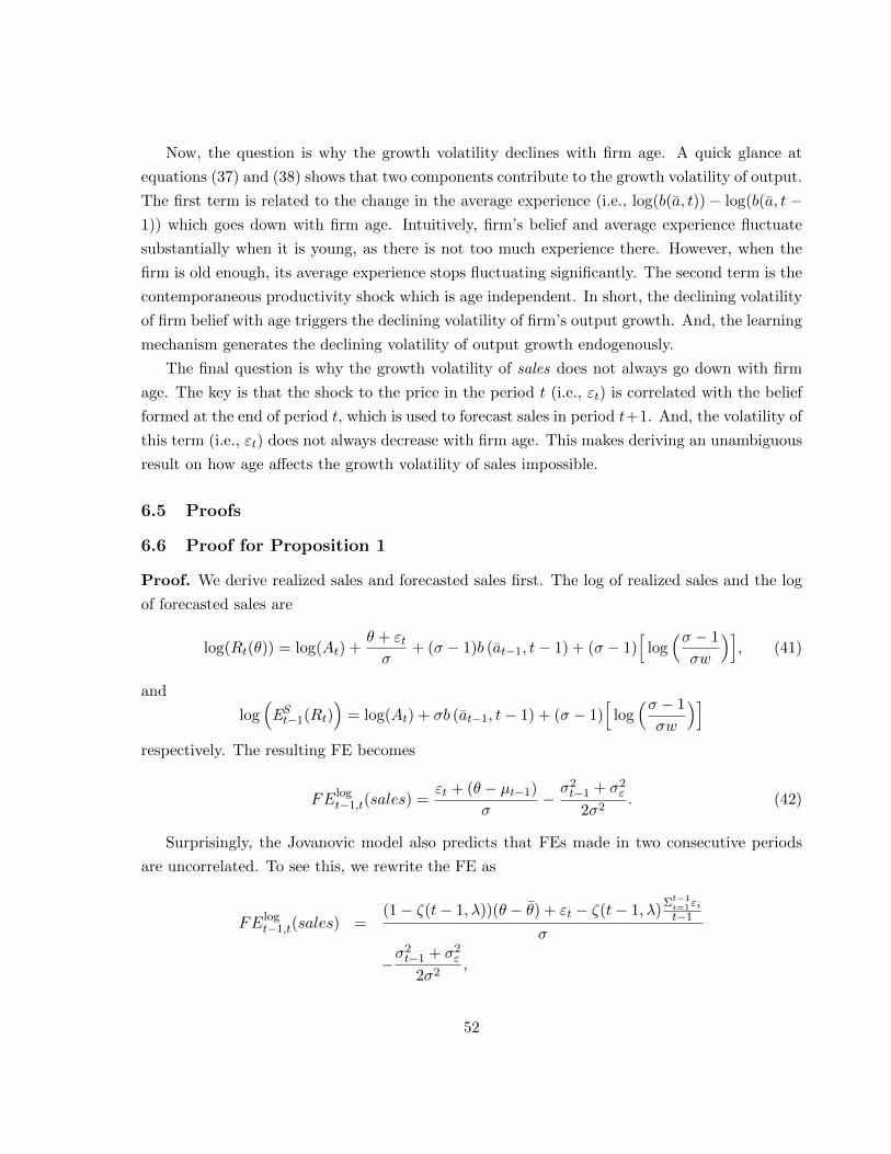
Now, the question is why the growth volatility declines with firm age. A quick glance at

equations (37) and (38) shows that two components contribute to the growth volatility of output.

The first term is related to the change in the average experience (i.e., log(b(a, t))− log(b(a, t−1)) which goes down with firm age. Intuitively, firm’s belief and average experience fluctuate

substantially when it is young, as there is not too much experience there. However, when the

firm is old enough, its average experience stops fluctuating significantly. The second term is the

contemporaneous productivity shock which is age independent. In short, the declining volatility

of firm belief with age triggers the declining volatility of firm’s output growth. And, the learning

mechanism generates the declining volatility of output growth endogenously.

The final question is why the growth volatility of sales does not always go down with firm

age. The key is that the shock to the price in the period t (i.e., εt) is correlated with the belief

formed at the end of period t, which is used to forecast sales in period t+1. And, the volatility of

this term (i.e., εt) does not always decrease with firm age. This makes deriving an unambiguous

result on how age affects the growth volatility of sales impossible.

6.5 Proofs

6.6 Proof for Proposition 1

Proof. We derive realized sales and forecasted sales first. The log of realized sales and the log

of forecasted sales are

log(Rt(θ)) = log(At) +θ + εtσ

+ (σ − 1)b (at−1, t− 1) + (σ − 1)[

log(σ − 1

σw

)], (41)

and

log(

ESt−1(Rt))

= log(At) + σb (at−1, t− 1) + (σ − 1)[

log(σ − 1

σw

)]respectively. The resulting FE becomes

FElogt−1,t(sales) =

εt + (θ − µt−1)

σ−σ2t−1 + σ2

ε

2σ2. (42)

Surprisingly, the Jovanovic model also predicts that FEs made in two consecutive periods

are uncorrelated. To see this, we rewrite the FE as

FElogt−1,t(sales) =

(1− ζ(t− 1, λ))(θ − θ) + εt − ζ(t− 1, λ)Σt−1i=1εit−1

σ

−σ2t−1 + σ2

ε

2σ2,

52

where the signal-to-noise ratio is defined as

λ ≡σ2θ

σ2ε

; ζ(t− 1, λ) ≡ (t− 1)λ

1 + (t− 1)λ.

The implied covariance of FEs in two consecutive periods is

cov(FElogt−1,t, FE

logt,t+1) =

1

σ2

[λσ2

ε

(1 + λt)(1 + λ(t− 1))− λtσ2

ε

t(1 + λt)+

λtλ(t− 1)σ2ε

t(1 + λt)(1 + λ(t− 1))

]= 0.

Readers are referred to Appendix 6.3 for the discussion of time-varying fundamental demand

draw.

6.6.1 Proof for Proposition 2

Proof. We can rewrite the expression of the variance of FE derived in the main text as:

var(FElogt−1,t(sales)) =

(1 + ζ(t−1,λ)2

t−1 )σ2ε

σ2+

(1− ζ(t− 1, λ))2σ2θ

σ2, (43)

where

ζ(t− 1, λ) ≡ (t− 1)λ

1 + (t− 1)λ.

Differentiating equation (43) with respect to t leads to

−∂ζ(t− 1, λ)

∂tσ2ε

[2(1− ζ(t− 1, λ))λ− 2ζ(t− 1, λ)

t− 1

]− σ2

ε

ζ(t− 1, λ)2

(t− 1)2,

which equals

−σ2ε

ζ(t− 1, λ)2

(t− 1)2< 0.

Therefore, variance of FEs declines with t.

53

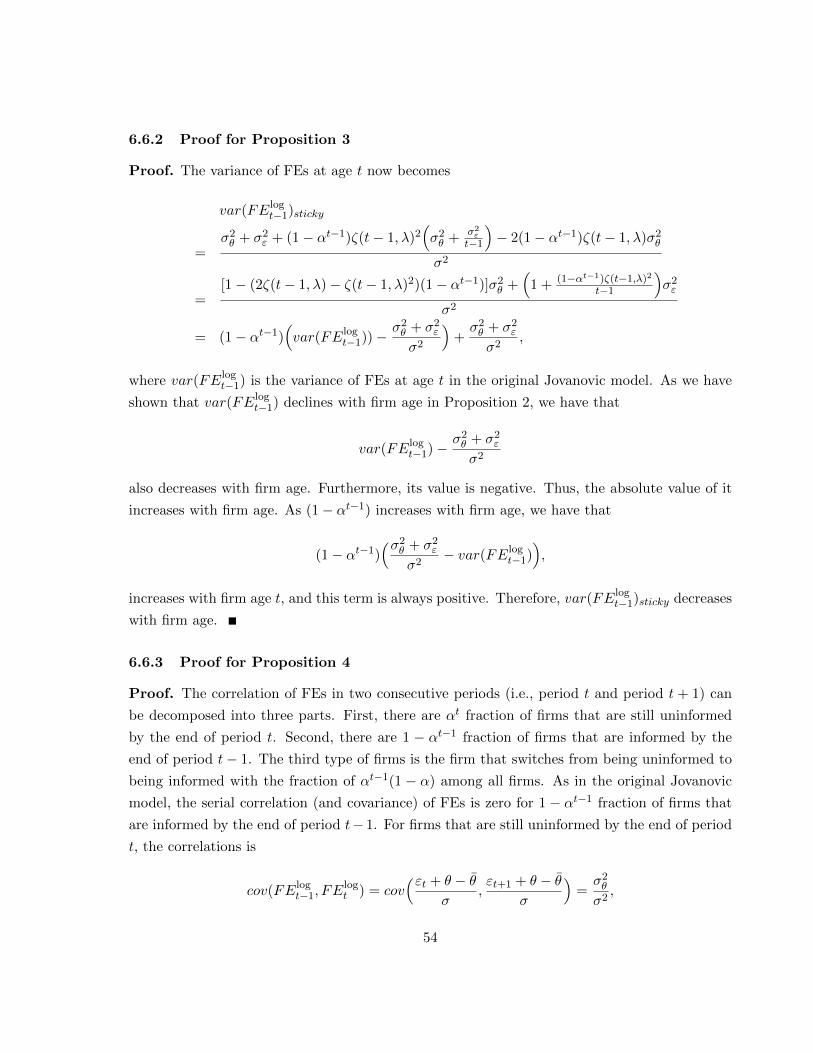
6.6.2 Proof for Proposition 3

Proof. The variance of FEs at age t now becomes

var(FElogt−1)sticky

=σ2θ + σ2

ε + (1− αt−1)ζ(t− 1, λ)2(σ2θ + σ2

εt−1

)− 2(1− αt−1)ζ(t− 1, λ)σ2

θ

σ2

=[1− (2ζ(t− 1, λ)− ζ(t− 1, λ)2)(1− αt−1)]σ2

θ +(

1 + (1−αt−1)ζ(t−1,λ)2

t−1

)σ2ε

σ2

= (1− αt−1)(var(FElog

t−1))−σ2θ + σ2

ε

σ2

)+σ2θ + σ2

ε

σ2,

where var(FElogt−1) is the variance of FEs at age t in the original Jovanovic model. As we have

shown that var(FElogt−1) declines with firm age in Proposition 2, we have that

var(FElogt−1)−

σ2θ + σ2

ε

σ2

also decreases with firm age. Furthermore, its value is negative. Thus, the absolute value of it

increases with firm age. As (1− αt−1) increases with firm age, we have that

(1− αt−1)(σ2

θ + σ2ε

σ2− var(FElog

t−1)),

increases with firm age t, and this term is always positive. Therefore, var(FElogt−1)sticky decreases

with firm age.

6.6.3 Proof for Proposition 4

Proof. The correlation of FEs in two consecutive periods (i.e., period t and period t + 1) can

be decomposed into three parts. First, there are αt fraction of firms that are still uninformed

by the end of period t. Second, there are 1 − αt−1 fraction of firms that are informed by the

end of period t− 1. The third type of firms is the firm that switches from being uninformed to

being informed with the fraction of αt−1(1 − α) among all firms. As in the original Jovanovic

model, the serial correlation (and covariance) of FEs is zero for 1 − αt−1 fraction of firms that

are informed by the end of period t− 1. For firms that are still uninformed by the end of period

t, the correlations is

cov(FElogt−1, FE

logt ) = cov

(εt + θ − θσ

,εt+1 + θ − θ

σ

)=σ2θ

σ2,

54

as they use the prior mean, θ, to forecast the fundamental demand in both periods. For the

switchers, the correlation is

cov(FElogt−1, FE

logt )

= cov(εt + θ − θ

σ,εt+1 + θ − µt

σ

)=

1

σ2cov(εt + θ − θ, θ − µt

)=

1

σ2cov(εt + θ − θ, θ − θ

1 + tλ−λ∑t

t=1 εt1 + tλ

)=

1

σ2

( σ2θ

1 + tλ− λσ2

ε

1 + tλ

)= 0.

Therefore, the average (total) covariance of FElogt−1,t and FElog

t,t+1 is

αtσ2θ

σ2,

which is strictly positive and decreases when firms become older. This is consistent with the

evidence presented in Table 7.

55

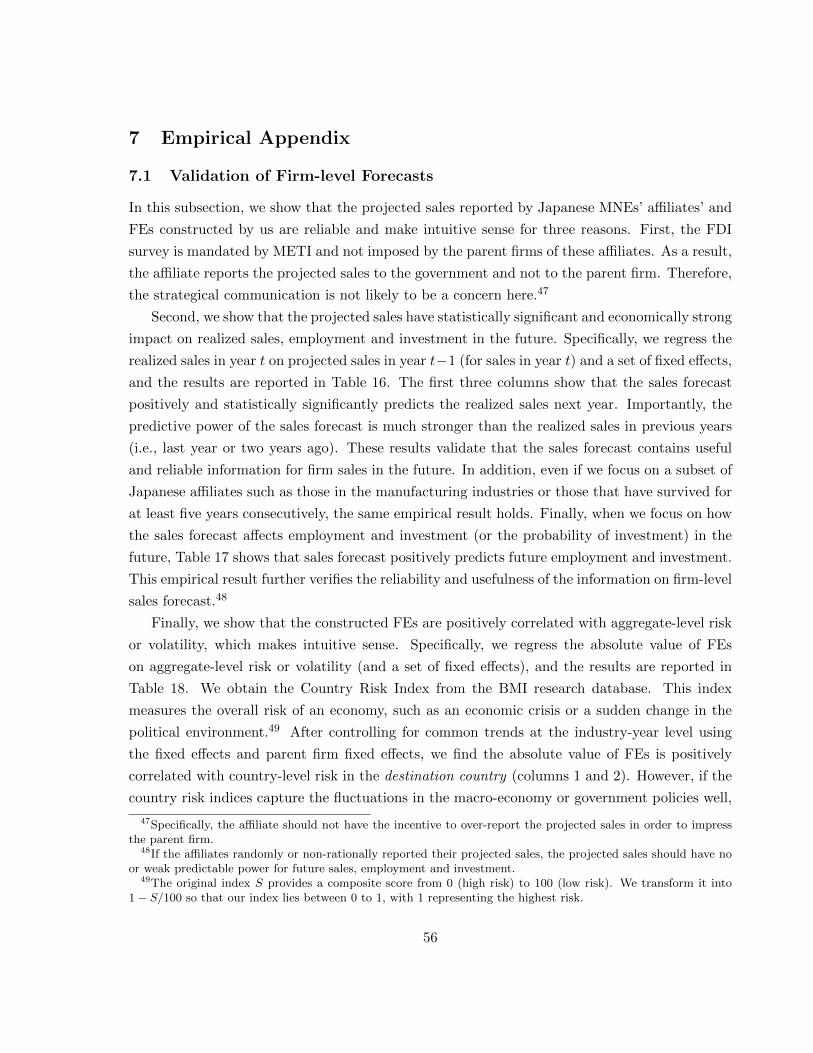
7 Empirical Appendix

7.1 Validation of Firm-level Forecasts

In this subsection, we show that the projected sales reported by Japanese MNEs’ affiliates’ and

FEs constructed by us are reliable and make intuitive sense for three reasons. First, the FDI

survey is mandated by METI and not imposed by the parent firms of these affiliates. As a result,

the affiliate reports the projected sales to the government and not to the parent firm. Therefore,

the strategical communication is not likely to be a concern here.47

Second, we show that the projected sales have statistically significant and economically strong

impact on realized sales, employment and investment in the future. Specifically, we regress the

realized sales in year t on projected sales in year t−1 (for sales in year t) and a set of fixed effects,

and the results are reported in Table 16. The first three columns show that the sales forecast

positively and statistically significantly predicts the realized sales next year. Importantly, the

predictive power of the sales forecast is much stronger than the realized sales in previous years

(i.e., last year or two years ago). These results validate that the sales forecast contains useful

and reliable information for firm sales in the future. In addition, even if we focus on a subset of

Japanese affiliates such as those in the manufacturing industries or those that have survived for

at least five years consecutively, the same empirical result holds. Finally, when we focus on how

the sales forecast affects employment and investment (or the probability of investment) in the

future, Table 17 shows that sales forecast positively predicts future employment and investment.

This empirical result further verifies the reliability and usefulness of the information on firm-level

sales forecast.48

Finally, we show that the constructed FEs are positively correlated with aggregate-level risk

or volatility, which makes intuitive sense. Specifically, we regress the absolute value of FEs

on aggregate-level risk or volatility (and a set of fixed effects), and the results are reported in

Table 18. We obtain the Country Risk Index from the BMI research database. This index

measures the overall risk of an economy, such as an economic crisis or a sudden change in the

political environment.49 After controlling for common trends at the industry-year level using

the fixed effects and parent firm fixed effects, we find the absolute value of FEs is positively

correlated with country-level risk in the destination country (columns 1 and 2). However, if the

country risk indices capture the fluctuations in the macro-economy or government policies well,

47Specifically, the affiliate should not have the incentive to over-report the projected sales in order to impressthe parent firm.

48If the affiliates randomly or non-rationally reported their projected sales, the projected sales should have noor weak predictable power for future sales, employment and investment.

49The original index S provides a composite score from 0 (high risk) to 100 (low risk). We transform it into1− S/100 so that our index lies between 0 to 1, with 1 representing the highest risk.

56

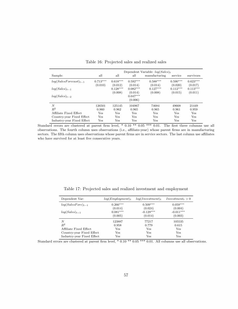
Table 16: Projected sales and realized sales

Dependent Variable: log(Sales)tSample: all all all manufacturing service survivors

log(SalesForecast)t−1 0.713∗∗∗ 0.618∗∗∗ 0.592∗∗∗ 0.588∗∗∗ 0.590∗∗∗ 0.623∗∗∗

(0.010) (0.012) (0.014) (0.014) (0.020) (0.017)log(Sales)t−1 0.128∗∗∗ 0.082∗∗∗ 0.127∗∗∗ 0.112∗∗∗ 0.113∗∗∗

(0.008) (0.014) (0.008) (0.015) (0.011)log(Sales)t−2 0.047∗∗∗

(0.006)

N 126501 125145 104967 74684 49668 21449R2 0.960 0.962 0.965 0.965 0.961 0.959Affiliate Fixed Effect Yes Yes Yes Yes Yes YesCountry-year Fixed Effect Yes Yes Yes Yes Yes YesIndustry-year Fixed Effect Yes Yes Yes Yes Yes Yes

Standard errors are clustered at parent firm level, * 0.10 ** 0.05 *** 0.01. The first three columns use allobservations. The fourth column uses observations (i.e., affiliate-year) whose parent firms are in manufacturingsectors. The fifth column uses observations whose parent firms are in service sectors. The last column use affiliateswho have survived for at least five consecutive years.

Table 17: Projected sales and realized investment and employment

Dependent Var: log(Employment)t log(Investment)t Investmentt > 0

log(SalesFore)t−1 0.266∗∗∗ 0.509∗∗∗ 0.059∗∗∗

(0.014) (0.024) (0.004)log(Sales)t−1 0.081∗∗∗ -0.129∗∗∗ -0.011∗∗∗

(0.005) (0.014) (0.003)

N 123887 77217 105535R2 0.958 0.779 0.615Affiliate Fixed Effect Yes Yes YesCountry-year Fixed Effect Yes Yes YesIndustry-year Fixed Effect Yes Yes Yes

Standard errors are clustered at parent firm level, * 0.10 ** 0.05 *** 0.01. All columns use all observations.

57

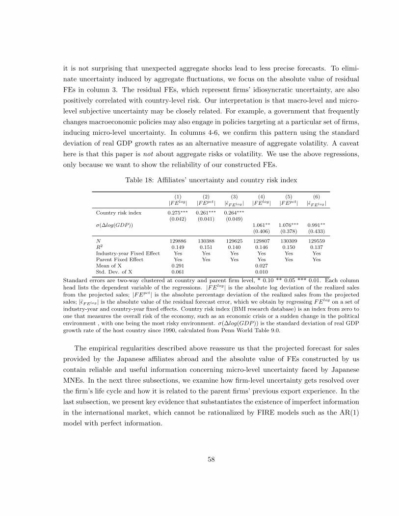
it is not surprising that unexpected aggregate shocks lead to less precise forecasts. To elimi-

nate uncertainty induced by aggregate fluctuations, we focus on the absolute value of residual

FEs in column 3. The residual FEs, which represent firms’ idiosyncratic uncertainty, are also

positively correlated with country-level risk. Our interpretation is that macro-level and micro-

level subjective uncertainty may be closely related. For example, a government that frequently

changes macroeconomic policies may also engage in policies targeting at a particular set of firms,

inducing micro-level uncertainty. In columns 4-6, we confirm this pattern using the standard

deviation of real GDP growth rates as an alternative measure of aggregate volatility. A caveat

here is that this paper is not about aggregate risks or volatility. We use the above regressions,

only because we want to show the reliability of our constructed FEs.

Table 18: Affiliates’ uncertainty and country risk index

(1) (2) (3) (4) (5) (6)|FElog | |FEpct| |εFElog | |FElog | |FEpct| |εFElog |

Country risk index 0.275∗∗∗ 0.261∗∗∗ 0.264∗∗∗

(0.042) (0.041) (0.049)σ(∆log(GDP )) 1.061∗∗ 1.076∗∗∗ 0.991∗∗

(0.406) (0.378) (0.433)

N 129886 130388 129625 129807 130309 129559R2 0.149 0.151 0.140 0.146 0.150 0.137Industry-year Fixed Effect Yes Yes Yes Yes Yes YesParent Fixed Effect Yes Yes Yes Yes Yes YesMean of X 0.291 0.027Std. Dev. of X 0.061 0.010

Standard errors are two-way clustered at country and parent firm level, * 0.10 ** 0.05 *** 0.01. Each columnhead lists the dependent variable of the regressions. |FElog| is the absolute log deviation of the realized salesfrom the projected sales; |FEpct| is the absolute percentage deviation of the realized sales from the projectedsales; |εFElog | is the absolute value of the residual forecast error, which we obtain by regressing FElog on a set ofindustry-year and country-year fixed effects. Country risk index (BMI research database) is an index from zero toone that measures the overall risk of the economy, such as an economic crisis or a sudden change in the politicalenvironment , with one being the most risky environment. σ(∆log(GDP )) is the standard deviation of real GDPgrowth rate of the host country since 1990, calculated from Penn World Table 9.0.

The empirical regularities described above reassure us that the projected forecast for sales

provided by the Japanese affiliates abroad and the absolute value of FEs constructed by us

contain reliable and useful information concerning micro-level uncertainty faced by Japanese

MNEs. In the next three subsections, we examine how firm-level uncertainty gets resolved over

the firm’s life cycle and how it is related to the parent firms’ previous export experience. In the

last subsection, we present key evidence that substantiates the existence of imperfect information

in the international market, which cannot be rationalized by FIRE models such as the AR(1)

model with perfect information.

58

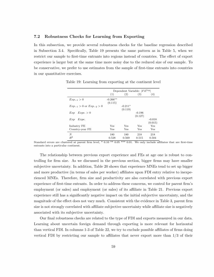
7.2 Robustness Checks for Learning from Exporting

In this subsection, we provide several robustness checks for the baseline regression described

in Subsection 3.4. Specifically, Table 19 presents the same pattern as in Table 5, when we

restrict our sample to first-time entrants into regions instead of countries. The effect of export

experience is larger but at the same time more noisy due to the reduced size of our sample. To

be conservative, we prefer to use estimates from the sample of first-time entrants into countries

in our quantitative exercises.

Table 19: Learning from exporting at the continent level

Dependent Variable: |FElog |(1) (2) (3) (4)

Exp−1 > 0 -0.266∗∗

(0.115)Exp−1 > 0 or Exp−2 > 0 -0.211∗

(0.119)Exp Expe. > 0 -0.196

(0.127)Exp Expe. -0.018

(0.015)Industry FE Yes Yes Yes YesCountry-year FE Yes Yes Yes Yes

N 180 180 218 218R2 0.528 0.569 0.515 0.504

Standard errors are clustered at parent firm level, * 0.10 ** 0.05 *** 0.01. We only include affiliates that are first-timeentrants into a particular continent.

The relationship between previous export experience and FEs at age one is robust to con-

trolling for firm size. As we discussed in the previous section, bigger firms may have smaller

subjective uncertainty. In addition, Table 20 shows that experience MNEs tend to set up bigger

and more productive (in terms of sales per worker) affiliates upon FDI entry relative to inexpe-

rienced MNEs. Therefore, firm size and productivity are also correlated with previous export

experience of first-time entrants. In order to address these concerns, we control for parent firm’s

employment (or sales) and employment (or sales) of its affiliate in Table 21. Previous export

experience still has a significantly negative impact on the initial subjective uncertainty, and the

magnitude of the effect does not vary much. Consistent with the evidence in Table 3, parent firm

size is not strongly correlated with affiliate subjective uncertainty while affiliate size is negatively

associated with its subjective uncertainty.

Our final robustness checks are related to the type of FDI and exports measured in our data.

Learning about uncertain foreign demand through exporting is more relevant for horizontal

than vertical FDI. In columns 1-3 of Table 22, we try to exclude possible affiliates of firms doing

vertical FDI by restricting our sample to affiliates that never export more than 1/3 of their

59

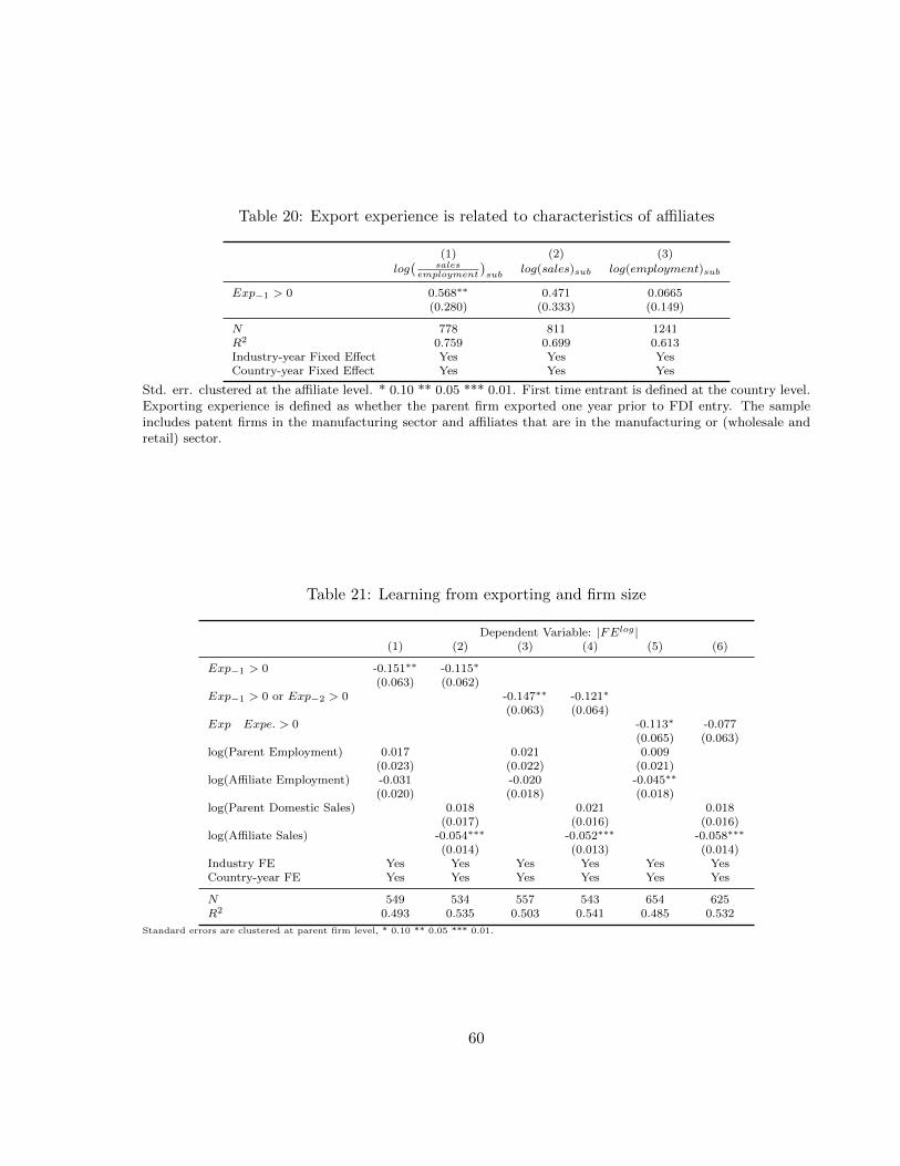
Table 20: Export experience is related to characteristics of affiliates

(1) (2) (3)

log(

salesemployment

)sub

log(sales)sub log(employment)sub

Exp−1 > 0 0.568∗∗ 0.471 0.0665(0.280) (0.333) (0.149)

N 778 811 1241R2 0.759 0.699 0.613Industry-year Fixed Effect Yes Yes YesCountry-year Fixed Effect Yes Yes Yes

Std. err. clustered at the affiliate level. * 0.10 ** 0.05 *** 0.01. First time entrant is defined at the country level.Exporting experience is defined as whether the parent firm exported one year prior to FDI entry. The sampleincludes patent firms in the manufacturing sector and affiliates that are in the manufacturing or (wholesale andretail) sector.

Table 21: Learning from exporting and firm size

Dependent Variable: |FElog |(1) (2) (3) (4) (5) (6)

Exp−1 > 0 -0.151∗∗ -0.115∗

(0.063) (0.062)Exp−1 > 0 or Exp−2 > 0 -0.147∗∗ -0.121∗

(0.063) (0.064)Exp Expe. > 0 -0.113∗ -0.077

(0.065) (0.063)log(Parent Employment) 0.017 0.021 0.009

(0.023) (0.022) (0.021)log(Affiliate Employment) -0.031 -0.020 -0.045∗∗

(0.020) (0.018) (0.018)log(Parent Domestic Sales) 0.018 0.021 0.018

(0.017) (0.016) (0.016)log(Affiliate Sales) -0.054∗∗∗ -0.052∗∗∗ -0.058∗∗∗

(0.014) (0.013) (0.014)Industry FE Yes Yes Yes Yes Yes YesCountry-year FE Yes Yes Yes Yes Yes Yes

N 549 534 557 543 654 625R2 0.493 0.535 0.503 0.541 0.485 0.532

Standard errors are clustered at parent firm level, * 0.10 ** 0.05 *** 0.01.

60

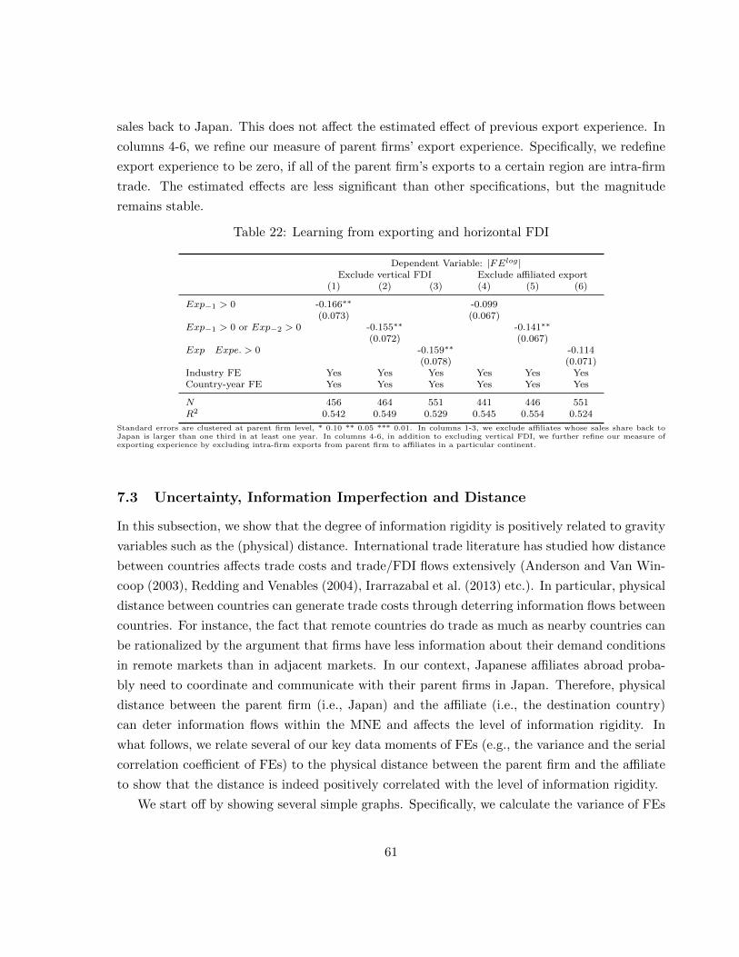
sales back to Japan. This does not affect the estimated effect of previous export experience. In

columns 4-6, we refine our measure of parent firms’ export experience. Specifically, we redefine

export experience to be zero, if all of the parent firm’s exports to a certain region are intra-firm

trade. The estimated effects are less significant than other specifications, but the magnitude

remains stable.

Table 22: Learning from exporting and horizontal FDI

Dependent Variable: |FElog |Exclude vertical FDI Exclude affiliated export

(1) (2) (3) (4) (5) (6)

Exp−1 > 0 -0.166∗∗ -0.099(0.073) (0.067)

Exp−1 > 0 or Exp−2 > 0 -0.155∗∗ -0.141∗∗

(0.072) (0.067)Exp Expe. > 0 -0.159∗∗ -0.114

(0.078) (0.071)Industry FE Yes Yes Yes Yes Yes YesCountry-year FE Yes Yes Yes Yes Yes Yes

N 456 464 551 441 446 551R2 0.542 0.549 0.529 0.545 0.554 0.524

Standard errors are clustered at parent firm level, * 0.10 ** 0.05 *** 0.01. In columns 1-3, we exclude affiliates whose sales share back toJapan is larger than one third in at least one year. In columns 4-6, in addition to excluding vertical FDI, we further refine our measure ofexporting experience by excluding intra-firm exports from parent firm to affiliates in a particular continent.

7.3 Uncertainty, Information Imperfection and Distance

In this subsection, we show that the degree of information rigidity is positively related to gravity

variables such as the (physical) distance. International trade literature has studied how distance

between countries affects trade costs and trade/FDI flows extensively (Anderson and Van Win-

coop (2003), Redding and Venables (2004), Irarrazabal et al. (2013) etc.). In particular, physical

distance between countries can generate trade costs through deterring information flows between

countries. For instance, the fact that remote countries do trade as much as nearby countries can

be rationalized by the argument that firms have less information about their demand conditions

in remote markets than in adjacent markets. In our context, Japanese affiliates abroad proba-

bly need to coordinate and communicate with their parent firms in Japan. Therefore, physical

distance between the parent firm (i.e., Japan) and the affiliate (i.e., the destination country)

can deter information flows within the MNE and affects the level of information rigidity. In

what follows, we relate several of our key data moments of FEs (e.g., the variance and the serial

correlation coefficient of FEs) to the physical distance between the parent firm and the affiliate

to show that the distance is indeed positively correlated with the level of information rigidity.

We start off by showing several simple graphs. Specifically, we calculate the variance of FEs

61

for all Japanese affiliates in a given economy at age one (i.e., FElog1,2) and above age ten (i.e.,

FElogt,t+1 where t ≥ 10) respectively. Since only a handful destination economies have enough

observations for us to calculate the variance of FEs for affiliates at age one, we end up with

Japanese affiliates in twenty major economies (excluding tax heaven economies) in our graph.50

We plot the variance of FEs for the two age cohorts in various economies against the weighted

distance from Japan (the data is obtained from CEPII) in Figures 7 and 8. It seems that the

initial uncertainty at the economy level is negatively related to the distance from Japan, while

the eventual uncertainty is uncorrelated to the distance.

The finding on the relationship between the initial uncertainty and distance is puzzling,

as the reader would think that Japanese affiliates in adjacent economies might have better

information about the destination markets and therefore have more precise forecasts than the

affiliates in remote economies. However, the fundamental volatility of the destination economy

(e.g., economic policy uncertainty, the probability of economic crisis and political uncertainty

etc.) probably plays a more important role than the level of information rigidity in determining

the precision of these affiliates’ forecasts. Note that economies close to Japan (e.g., China,

Taiwan and Southeast Asian countries) are emerging markets whose economic environment is

less stable than economies that are far away from Japan (e.g., the U.S., Canada, Australia and

European countries).51 This probably causes less precise forecasts made by Japanese affiliates

in Asian economies than those in north America and Europe.

What is interesting is that when we focus on the serial correlation coefficient of FEs over time,

which is a measure of the degree of information rigidity (and not for the fundamental volatility

of the economy), there is a strong positive association between the distance from Japan and

the level of the correlation for the destination economy. Figures 9 and 10 clearly show this

pattern. In other words, Japanese affiliates in China and Southeast Asia made less systematic

FEs compared to those in North America and Europe. In summary, the two empirical findings

above help us distinguish imperfect information across borders from volatility (or risks) of the

destination economies. This difference is economically important, as volatility is fundamentally

different from barriers to information flows.

Finally, we run the following panel regressions to confirm our finding on the relationship

between distance and the degree of information rigidity:

|FElog|it = distancec + log(sales)it + δc + δst +HQj(i) + δt + εit

50We want to have enough observations in the calculation, as otherwise the law of large numbers would nothold for each destination country. The twenty economies we pick have at least twenty observations of Japaneseaffiliates’ FEs at age one.

51We do not have many observations from economies in the middle east, Africa and South America.

62

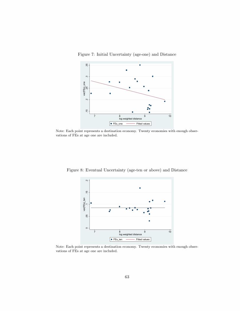
Figure 7: Initial Uncertainty (age-one) and Distance

.15

.2.2

5.3

.35

var(F

Es)_

one

7 8 9 10log weighted distance

FEs_one Fitted values

Note: Each point represents a destination economy. Twenty economies with enough obser-vations of FEs at age one are included.

Figure 8: Eventual Uncertainty (age-ten or above) and Distance

0.0

5.1

.15

.2va

r(FEs

)_te

n

7 8 9 10log weighted distance

FEs_ten Fitted values

Note: Each point represents a destination economy. Twenty economies with enough obser-vations of FEs at age one are included.

63

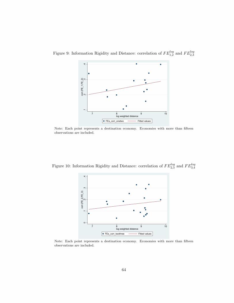
Figure 9: Information Rigidity and Distance: correlation of FElog1,2 and FElog2,3

.1.2

.3.4

corr.

(FE_

1,FE

_2)

7 8 9 10log weighted distance

FEs_corr_onetwo Fitted values

Note: Each point represents a destination economy. Economies with more than fifteenobservations are included.

Figure 10: Information Rigidity and Distance: correlation of FElog2,3 and FElog3,4

0.1

.2.3

.4co

rr.(F

E_2,

FE_3

)

7 8 9 10log weighted distance

FEs_corr_twothree Fitted values

Note: Each point represents a destination economy. Economies with more than fifteenobservations are included.

64

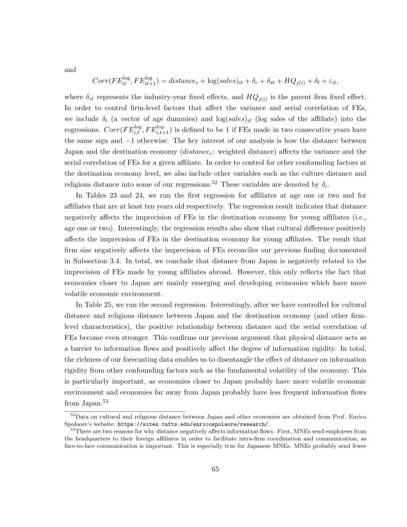
and

Corr(FElogit , FE

logit+1) = distancec + log(sales)it + δc + δst +HQj(i) + δt + εit,

where δst represents the industry-year fixed effects, and HQj(i) is the parent firm fixed effect.

In order to control firm-level factors that affect the variance and serial correlation of FEs,

we include δt (a vector of age dummies) and log(sales)it (log sales of the affiliate) into the

regressions. Corr(FElogi,t , FElogi,t+1) is defined to be 1 if FEs made in two consecutive years have

the same sign and −1 otherwise. The key interest of our analysis is how the distance between

Japan and the destination economy (distancec: weighted distance) affects the variance and the

serial correlation of FEs for a given affiliate. In order to control for other confounding factors at

the destination economy level, we also include other variables such as the culture distance and

religious distance into some of our regressions.52 These variables are denoted by δc.

In Tables 23 and 24, we run the first regression for affiliates at age one or two and for

affiliates that are at least ten years old respectively. The regression result indicates that distance

negatively affects the imprecision of FEs in the destination economy for young affiliates (i.e.,

age one or two). Interestingly, the regression results also show that cultural difference positively

affects the imprecision of FEs in the destination economy for young affiliates. The result that

firm size negatively affects the imprecision of FEs reconciles our previous finding documented

in Subsection 3.4. In total, we conclude that distance from Japan is negatively related to the

imprecision of FEs made by young affiliates abroad. However, this only reflects the fact that

economies closer to Japan are mainly emerging and developing economies which have more

volatile economic environment.

In Table 25, we run the second regression. Interestingly, after we have controlled for cultural

distance and religious distance between Japan and the destination economy (and other firm-

level characteristics), the positive relationship between distance and the serial correlation of

FEs become even stronger. This confirms our previous argument that physical distance acts as

a barrier to information flows and positively affect the degree of information rigidity. In total,

the richness of our forecasting data enables us to disentangle the effect of distance on information

rigidity from other confounding factors such as the fundamental volatility of the economy. This

is particularly important, as economies closer to Japan probably have more volatile economic

environment and economies far away from Japan probably have less frequent information flows

from Japan.53

52Data on cultural and religious distance between Japan and other economies are obtained from Prof. EnricoSpolaore’s website: https://sites.tufts.edu/enricospolaore/research/.

53There are two reasons for why distance negatively affects information flows. First, MNEs send employees fromthe headquarters to their foreign affiliates in order to facilitate intra-firm coordination and communication, asface-to-face communication is important. This is especially true for Japanese MNEs. MNEs probably send fewer

65

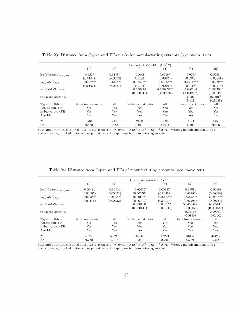
Table 23: Distance from Japan and FEs made by manufacturing entrants (age one or two)

Dependent Variable: |FElog |(1) (2) (3) (4) (5) (6)

log(distance)weighted -0.0227 -0.0155∗ -0.0198 -0.0209∗∗ -0.0295 -0.0253∗∗

(0.0144) (0.00633) (0.0193) (0.00724) (0.0290) (0.00841)log(sales)sub -0.0777∗∗∗ -0.0615∗∗∗ -0.0753∗∗∗ -0.0586∗∗∗ -0.0716∗∗∗ -0.0582∗∗∗

(0.0102) (0.00454) (0.0105) (0.00464) (0.0103) (0.00475)cultural distance 0.000354 0.000858∗∗ 0.000344 0.000709∗

(0.000841) (0.000294) (0.000967) (0.000325)religious distance 0.124 0.0801+

(0.111) (0.0456)Type of affiliate first-time entrants all first-time entrants all first-time entrants allParent firm FE Yes Yes Yes Yes Yes YesIndustry-year FE Yes Yes Yes Yes Yes YesAge FE Yes Yes Yes Yes Yes Yes

N 2564 5201 2198 4594 2123 4459R2 0.660 0.483 0.689 0.502 0.694 0.506

Standard errors are clustered at the destination country level, + 0.10 * 0.05 ** 0.01 *** 0.001. We only include manufacturingand wholesale/retail affiliates whose parent firms in Japan are in manufacturing sectors.

Table 24: Distance from Japan and FEs of manufacturing entrants (age above ten)

Dependent Variable: |FElog |(1) (2) (3) (4) (5) (6)

log(distance)weighted -0.00431 -0.00314 -0.00557 -0.00537+ -0.00511 -0.00663(0.00305) (0.00322) (0.00350) (0.00302) (0.00461) (0.00395)

log(sales)sub -0.0233∗∗∗ -0.0205∗∗∗ -0.0226∗∗∗ -0.0205∗∗∗ -0.0225∗∗∗ -0.0206∗∗∗

(0.00177) (0.00122) (0.00191) (0.00130) (0.00203) (0.00137)cultural distance 0.000110 0.000155 0.0000992 0.000143

(0.000141) (0.000110) (0.000153) (0.000131)religious distance -0.00159 0.00983

(0.0143) (0.0160)Type of affiliate first-time entrants all first-time entrants all first-time entrants allParent firm FE Yes Yes Yes Yes Yes YesIndustry-year FE Yes Yes Yes Yes Yes YesAge FE Yes Yes Yes Yes Yes Yes

N 40750 56390 34044 47229 31857 44423R2 0.230 0.197 0.246 0.209 0.250 0.213

Standard errors are clustered at the destination country level, + 0.10 * 0.05 ** 0.01 *** 0.001. We only include manufacturingand wholesale/retail affiliates whose parent firms in Japan are in manufacturing sectors.

66

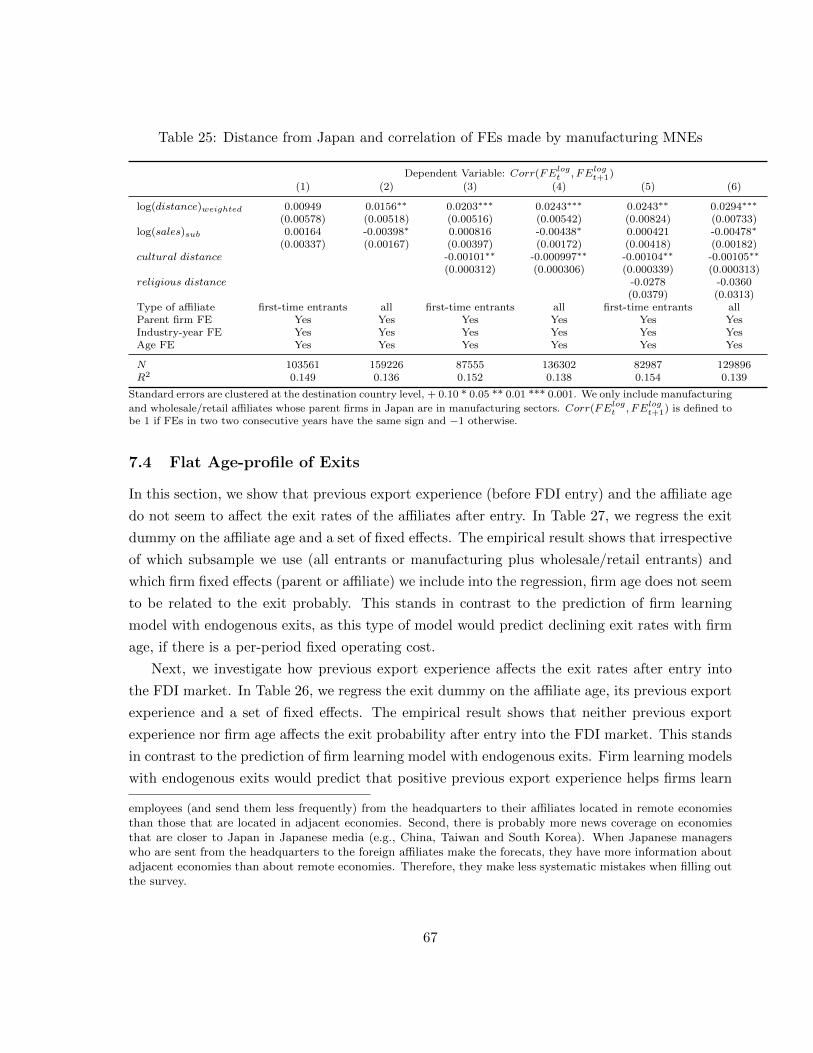
Table 25: Distance from Japan and correlation of FEs made by manufacturing MNEs

Dependent Variable: Corr(FElogt , FElogt+1)

(1) (2) (3) (4) (5) (6)

log(distance)weighted 0.00949 0.0156∗∗ 0.0203∗∗∗ 0.0243∗∗∗ 0.0243∗∗ 0.0294∗∗∗

(0.00578) (0.00518) (0.00516) (0.00542) (0.00824) (0.00733)log(sales)sub 0.00164 -0.00398∗ 0.000816 -0.00438∗ 0.000421 -0.00478∗

(0.00337) (0.00167) (0.00397) (0.00172) (0.00418) (0.00182)cultural distance -0.00101∗∗ -0.000997∗∗ -0.00104∗∗ -0.00105∗∗

(0.000312) (0.000306) (0.000339) (0.000313)religious distance -0.0278 -0.0360

(0.0379) (0.0313)Type of affiliate first-time entrants all first-time entrants all first-time entrants allParent firm FE Yes Yes Yes Yes Yes YesIndustry-year FE Yes Yes Yes Yes Yes YesAge FE Yes Yes Yes Yes Yes Yes

N 103561 159226 87555 136302 82987 129896R2 0.149 0.136 0.152 0.138 0.154 0.139

Standard errors are clustered at the destination country level, + 0.10 * 0.05 ** 0.01 *** 0.001. We only include manufacturing

and wholesale/retail affiliates whose parent firms in Japan are in manufacturing sectors. Corr(FElogt , FElogt+1) is defined tobe 1 if FEs in two two consecutive years have the same sign and −1 otherwise.

7.4 Flat Age-profile of Exits

In this section, we show that previous export experience (before FDI entry) and the affiliate age

do not seem to affect the exit rates of the affiliates after entry. In Table 27, we regress the exit

dummy on the affiliate age and a set of fixed effects. The empirical result shows that irrespective

of which subsample we use (all entrants or manufacturing plus wholesale/retail entrants) and

which firm fixed effects (parent or affiliate) we include into the regression, firm age does not seem

to be related to the exit probably. This stands in contrast to the prediction of firm learning

model with endogenous exits, as this type of model would predict declining exit rates with firm

age, if there is a per-period fixed operating cost.

Next, we investigate how previous export experience affects the exit rates after entry into

the FDI market. In Table 26, we regress the exit dummy on the affiliate age, its previous export

experience and a set of fixed effects. The empirical result shows that neither previous export

experience nor firm age affects the exit probability after entry into the FDI market. This stands

in contrast to the prediction of firm learning model with endogenous exits. Firm learning models

with endogenous exits would predict that positive previous export experience helps firms learn

employees (and send them less frequently) from the headquarters to their affiliates located in remote economiesthan those that are located in adjacent economies. Second, there is probably more news coverage on economiesthat are closer to Japan in Japanese media (e.g., China, Taiwan and South Korea). When Japanese managerswho are sent from the headquarters to the foreign affiliates make the forecats, they have more information aboutadjacent economies than about remote economies. Therefore, they make less systematic mistakes when filling outthe survey.

67

Table 26: Age profile of affiliates’ exiting

Dependent Variable: exit dummy(1) (2) (3) (4)

affiliate age 0.0000382 0.0000312 -0.0000612 -0.0000668(0.0000551) (0.0000562) (0.0000570) (0.0000582)

Affiliate type manuf.+wholesale/retail manuf.+wholesale/retail all allAffiliate FE Yes No Yes NoParent firm FE No Yes No YesIndustry-year FE Yes Yes Yes YesCountry-year FE Yes Yes Yes Yes

N 94273 94271 125947 125941R2 0.099 0.101 0.107 0.108

Standard errors are clustered at the affiliate level, + 0.10 * 0.05 ** 0.01 *** 0.001. Only first-time entrants into thedestination markets are included.

about their demand and reduce exit rates after entry, if there is a per-period fixed operating

cost which triggers endogenous exits.

Table 27: Export experience and exiting probability of the affiliates

Dependent Variable: exit dummy(1) (2)

Exp−1 > 0 0.00205 0.00222(0.0134) (0.0132)

affiliate age 0.000527 0.000571(0.000777) (0.000771)

One-parent-one-affiliate pairs included? No YesParent firm FE Yes YesIndustry-year FE Yes YesCountry-year FE Yes Yes

N 6202 7913R2 0.223 0.235

Standard errors are clustered at the affiliate level, + 0.10 * 0.05 ** 0.01 *** 0.001. We only include manufacturing andwholesale/retail affiliates whose parent firms in Japan are in manufacturing sectors. Only first-time entrants into thedestination markets are included.

In total, as we do not observe significant effects of previous export experience and firm age

on the exit rates after FDI entry, there is no strong sign for the existence of endogenous exits

among multinational affiliates in our dataset. Therefore, we set the per-period fixed operating

cost of FDI, fm = 0, to zero in our calibration exercise.

68

References

Abel, Andrew B., “Optimal investment under uncertainty,” The American Economic Review,

1983, 73 (1), 228–233.

and Janice C. Eberly, “Optimal investment with costly reversibility,” The Review of

Economic Studies, 1996, 63 (4), 581–593.

Aeberhardt, Romain, Ines Buono, and Harald Fadinger, “Learning, incomplete contracts

and export dynamics: Theory and evidence from French firms,” European Economic Review,

May 2014, 68, 219–249.

Akhmetova, Zhanar and Cristina Mitaritonna, “A Model of Firm Experimentation un-

der Demand Uncertainty: an Application to Multi-Destination Exporters,” Working Paper,

CEPII research center April 2013.

Albornoz, Facundo, Hector F. Calvo Pardo, Gregory Corcos, and Emanuel Ornelas,

“Sequential exporting,” Journal of International Economics, 2012, 88 (1), 17–31.

Anderson, James E and Eric Van Wincoop, “Gravity with gravitas: a solution to the

border puzzle,” the american economic review, 2003, 93 (1), 170–192.

Andrade, Philippe and Herve Le Bihan, “Inattentive professional forecasters,” Journal of

Monetary Economics, 2013, 60 (8), 967–982.

Arkolakis, Costas, Natalia Ramondo, Andres Rodrıguez-Clare, and Stephen Yeaple,

“Innovation and Production in the Global Economy,” Working Paper 18972, National Bureau

of Economic Research April 2013.

, Theodore Papageorgiou, and Olga Timoshenko, “Firm Learning and Growth,” Work-

ing Paper 2017.

Bachmann, Rudiger and Christian Bayer, “Investment Dispersion and the Business Cy-

cle,” American Economic Review, April 2014, 104 (4), 1392–1416.

, Steffen Elstner, and Eric R Sims, “Uncertainty and Economic Activity: Evidence from

Business Survey Data,” American Economic Journal: Macroeconomics, April 2013, 5 (2),

217–249.

Bachmann, Ruediger, Steffen Elstner, and Atanas Hristov, “Surprise, surprise–

Measuring firm-level investment innovations,” Journal of Economic Dynamics and Control,

2017, 83, 107–148.

69

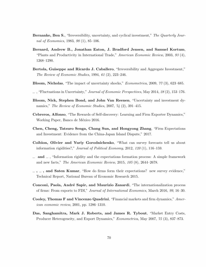
Bernanke, Ben S., “Irreversibility, uncertainty, and cyclical investment,” The Quarterly Jour-

nal of Economics, 1983, 98 (1), 85–106.

Bernard, Andrew B., Jonathan Eaton, J. Bradford Jensen, and Samuel Kortum,

“Plants and Productivity in International Trade,” American Economic Review, 2003, 93 (4),

1268–1290.

Bertola, Guiseppe and Ricardo J. Caballero, “Irreversibility and Aggregate Investment,”

The Review of Economic Studies, 1994, 61 (2), 223–246.

Bloom, Nicholas, “The impact of uncertainty shocks,” Econometrica, 2009, 77 (3), 623–685.

, “Fluctuations in Uncertainty,” Journal of Economic Perspectives, May 2014, 28 (2), 153–176.

Bloom, Nick, Stephen Bond, and John Van Reenen, “Uncertainty and investment dy-

namics,” The Review of Economic Studies, 2007, 74 (2), 391–415.

Cebreros, Alfonso, “The Rewards of Self-discovery: Learning and Firm Exporter Dynamics,”

Working Paper, Banco de Mexico 2016.

Chen, Cheng, Tatsuro Senga, Chang Sun, and Hongyong Zhang, “Firm Expectations

and Investment: Evidence from the China-Japan Island Dispute,” 2017.

Coibion, Olivier and Yuriy Gorodnichenko, “What can survey forecasts tell us about

information rigidities?,” Journal of Political Economy, 2012, 120 (1), 116–159.

and , “Information rigidity and the expectations formation process: A simple framework

and new facts,” The American Economic Review, 2015, 105 (8), 2644–2678.

, , and Saten Kumar, “How do firms form their expectations? new survey evidence,”

Technical Report, National Bureau of Economic Research 2015.

Conconi, Paola, Andre Sapir, and Maurizio Zanardi, “The internationalization process

of firms: From exports to FDI,” Journal of International Economics, March 2016, 99, 16–30.

Cooley, Thomas F and Vincenzo Quadrini, “Financial markets and firm dynamics,” Amer-

ican economic review, 2001, pp. 1286–1310.

Das, Sanghamitra, Mark J. Roberts, and James R. Tybout, “Market Entry Costs,

Producer Heterogeneity, and Export Dynamics,” Econometrica, May 2007, 75 (3), 837–873.

70

Deseatnicov, Ivan and Konstantin Kucheryavyy, “Exports and FDI Entry Decision: Ev-

idence from Japanese foreign-affiliated firms,” Working Paper 17-E-036, RIETI March 2017.

Dickstein, Michael J. and Eduardo Morales, “What do Exporters Know?,” Working Paper

2016.

Dixit, Avinash K. and Robert S. Pindyck, Investment under uncertainty, Princeton uni-

versity press, 1994.

Dominguez, Kathryn M, “Are foreign exchange forecasts rational?: New evidence from

survey data,” Economics Letters, 1986, 21 (3), 277–281.

Eaton, Jonathan and Samuel Kortum, “Technology, Geography, and Trade,” Economet-

rica, 2002, 70 (5), 1741–1779.

Eslava, Marcela, James Tybout, David Jinkins, Cornell J. Krizan, and Jonathan

Eaton, “A search and learning model of export dynamics,” Technical Report 2015.

Fillat, Jose L. and Stefania Garetto, “Risk, Returns, and Multinational Production,” The

Quarterly Journal of Economics, September 2015.

Fitzgerald, Doireann, Stefanie Haller, and Yaniv Yedid-Levi, “How Exporters Grow,”

Working Paper 2016.

Guiso, Luigi and Giuseppe Parigi, “Investment and Demand Uncertainty,” The Quarterly

Journal of Economics, February 1999, 114 (1), 185–227.

Gumpert, Anna, Andreas Moxnes, Natalia Ramondo, and Felix Tintelnot, “Multi-

national Firms and Export Dynamics,” Working Paper 2016.

Handley, Kyle, “Exporting under trade policy uncertainty: Theory and evidence,” Journal of

international Economics, 2014, 94 (1), 50–66.

and Nuno Limao, “Trade and Investment under Policy Uncertainty: Theory and Firm

Evidence,” American Economic Journal: Economic Policy, November 2015, 7 (4), 189–222.

and Nuno Limao, “Policy Uncertainty, Trade and Welfare: Theory and Evidence for China

and the U.S,” Working Paper 2017.

Helpman, Elhanan, Marc J. Melitz, and Stephen R. Yeaple, “Export versus FDI with

Heterogeneous Firms,” The American Economic Review, March 2004, 94 (1), 300–316.

71

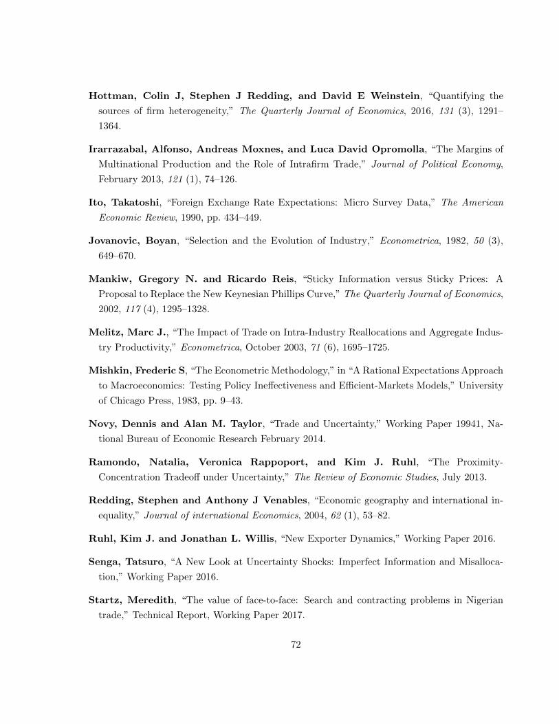
Hottman, Colin J, Stephen J Redding, and David E Weinstein, “Quantifying the

sources of firm heterogeneity,” The Quarterly Journal of Economics, 2016, 131 (3), 1291–

1364.

Irarrazabal, Alfonso, Andreas Moxnes, and Luca David Opromolla, “The Margins of

Multinational Production and the Role of Intrafirm Trade,” Journal of Political Economy,

February 2013, 121 (1), 74–126.

Ito, Takatoshi, “Foreign Exchange Rate Expectations: Micro Survey Data,” The American

Economic Review, 1990, pp. 434–449.

Jovanovic, Boyan, “Selection and the Evolution of Industry,” Econometrica, 1982, 50 (3),

649–670.

Mankiw, Gregory N. and Ricardo Reis, “Sticky Information versus Sticky Prices: A

Proposal to Replace the New Keynesian Phillips Curve,” The Quarterly Journal of Economics,

2002, 117 (4), 1295–1328.

Melitz, Marc J., “The Impact of Trade on Intra-Industry Reallocations and Aggregate Indus-

try Productivity,” Econometrica, October 2003, 71 (6), 1695–1725.

Mishkin, Frederic S, “The Econometric Methodology,” in “A Rational Expectations Approach

to Macroeconomics: Testing Policy Ineffectiveness and Efficient-Markets Models,” University

of Chicago Press, 1983, pp. 9–43.

Novy, Dennis and Alan M. Taylor, “Trade and Uncertainty,” Working Paper 19941, Na-

tional Bureau of Economic Research February 2014.

Ramondo, Natalia, Veronica Rappoport, and Kim J. Ruhl, “The Proximity-

Concentration Tradeoff under Uncertainty,” The Review of Economic Studies, July 2013.

Redding, Stephen and Anthony J Venables, “Economic geography and international in-

equality,” Journal of international Economics, 2004, 62 (1), 53–82.

Ruhl, Kim J. and Jonathan L. Willis, “New Exporter Dynamics,” Working Paper 2016.

Senga, Tatsuro, “A New Look at Uncertainty Shocks: Imperfect Information and Misalloca-

tion,” Working Paper 2016.

Startz, Meredith, “The value of face-to-face: Search and contracting problems in Nigerian

trade,” Technical Report, Working Paper 2017.

72

Timoshenko, Olga A., “Learning versus sunk costs explanations of export persistence,” Eu-

ropean Economic Review, October 2015, 79, 113–128.

73