uncertainties in hydraulic transient modelling in raising pipe systems: laboratory case studies

Procedia Engineering 70 ( 2014 ) 487 – 496

Available online at www.sciencedirect.com

1877-7058 © 2013 The Authors. Published by Elsevier Ltd. Selection and peer-review under responsibility of the CCWI2013 Committeedoi: 10.1016/j.proeng.2014.02.054

ScienceDirect

12th International Conference on Computing and Control for the Water Industry, CCWI2013

Uncertainties in hydraulic transient modelling in raising pipe systems: laboratory case studies

J.N. Delgadoa, N.M.C. Martinsa, D.I.C. Covasa, *a Instituto Superior Técnico, Lisbon, Portugal

Abstract

The current paper aims to discuss the main uncertainties associated with the hydraulic transient modelling of raising pipe systems with and without surge protection. A one-dimensional hydraulic transient solver was developed based on the classic water hammer theory and solved by the Method of Characteristics (MOC). The solver incorporates the pump-element described by Suter parameters, a pressurised surge tank (hydropneumatic vessel, HPV) and Vitkovsky’s (2000) formula for unsteady friction description. The model was tested using transient pressure data and steady-state flow data from two hydraulic circuits installed at the Hydraulics Laboratory of the Civil Engineering Department, in Instituto Superior Tecnico (Lisbon, Portugal). Pressure data were obtained at two/three locations (at the upstream end, at a middle section and at the downstream end). Transient tests with and without the HPV connected to the system were carried out for different flow rates. Transients were generated by the sudden stoppage of the pump. Collected data were compared with the results of the numerical modelling and used to calibrate model parameters. Good agreement between data and numerical results was obtained. Some tests with the HPV connected lead to higher pressure surges than when there was no protection in the system. These analyses are important to develop more solid and reliable numerical models as well to create awareness of the main uncertainties of developed models. © 2013 The Authors. Published by Elsevier Ltd. Selection and peer-review under responsibility of the CCWI2013 Committee.

Keywords: Hydraulic transient, surge protection, raising sustem, hydropneumatic vessel, unsteady friction.

* Corresponding author. Tel.: +351-218-417-000; fax: +351-218-499-242. E-mail address: [email protected]

© 2013 The Authors. Published by Elsevier Ltd. Selection and peer-review under responsibility of the CCWI2013 Committee

http://crossmark.crossref.org/dialog/?doi=10.1016/j.proeng.2014.02.054&domain=pdf

http://crossmark.crossref.org/dialog/?doi=10.1016/j.proeng.2014.02.054&domain=pdf

488 J.N. Delgado et al. / Procedia Engineering 70 ( 2014 ) 487 – 496

1. Introduction

The control of hydraulic transients in pressurized water supply and wastewater systems is a major concern for engineers and pipe system managers, for reasons related to risk, safety and efficient operation. Examples of problems caused by hydraulic transients are the occurrence of instabilities in the operation of systems due to the transient sub-atmospheric pressures and, consequently, the occurrence of cavitation, or the pipe burst due to the occurrence of overpressures. Hydraulic transients can be analyzed by means of simplified formulas (e.g., Joukowsky and Michaud formulas), classic water hammer simulators (e.g., commercial models) and by using more complete simulators (non-conventional models). Typically, results obtained by the commercial models, although based on classic water hammer, are satisfactory in terms of design of pressurized pipe systems, as maximum and minimum pressures occurred in the systems can be reasonably well estimated and surge protection devices can be designed whenever necessary to control transient pressures. However, these models are not accurate enough for the diagnosis and analysis of existing systems, mainly because these models cannot describe unconventional phenomena, such as cavitation, two-phase flow, unsteady friction and nonlinear rheological behavior of the pipe; in these cases, it is necessary to use more complex models incorporating the full description of these phenomena, which are not commercially available and which are much more model calibration-dependent.

The current paper aims at the experimental and numerical analysis of the pipe flow behavior during transient events carried out in two experimental facilities under controlled laboratory conditions, at the Hydraulic Laboratory of the Civil Engineering Department of Technical Institute of Lisbon (Lisbon, Portugal). The paper includes a brief description of the developed hydraulic transient solver, the description of the experimental facilities used and the set of experimental tests carried out, and the comparison of experimental tests and the mathematical model results. Finally, the main uncertainties associated with these hydraulic transients modeling are discussed.

2. Experimental facilities and data collection

2.1. Copper Pipeline

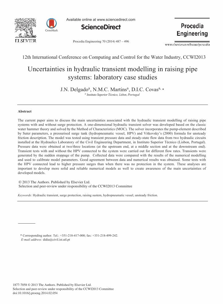
An experimental pipe rig was assembled in the Laboratory of Hydraulics and Water Resources, in Department of Civil Engineering and Architecture (DECivil), at Instituto Superior Técnico (IST), for analysis of transient events both for academic (i.e., lecturing under/postgraduate courses) and research purposes (Figure 1a). The pipe rig has a simple configuration of the type “reservoir-pipe-valve”. The pipe is made of coiled cooper with approximately 100 m of length, 20 mm of inner diameter and 1 mm of pipe-wall thickness. The system is supplied from a storage tank with 125 l of capacity by pump with nominal flow rate of 4.5 m3h-1 and nominal head of 43 m. The rig was assembled with a portable metal frame (with four wheels), 1 m depth, 2 m length and 1.6 m height, for lecturing purposes in undergraduate and post-graduate courses.

Immediately at downstream of the pump, there is a hydro-pneumatic vessel (HPV), made of stainless steel, with 60 l of capacity and designed for the nominal pressure of 6 bar (Figure 1b). At the upstream end there is a set of valves for changing the system configuration, which allows three different configurations: (I) Tank–pump–pipe– HPV (bifurcation)–pipe–valve; (II) Tank–pump–HPV–pipe–valve; and (III) Tank–pump–pipe–valve. At the downstream end of the pipe, there is a system of valves – a ball valve with DN 3/4’’ and globe valve with DN15 ½ – that allow the generation of water hammer and the control of the flow rate, respectively.

The facility is equipped with instrumentation for collecting steady flow data and transient pressure data. Steady state flow rates are measured by a rotameter and transient pressures are measured by three strain-gauge type pressure transducers located in different sections of the pipe (T1): at the upstream end, T2: at a middle section and T3: at the downstream end) and using a data acquisition system (Picoscope) with four channels.

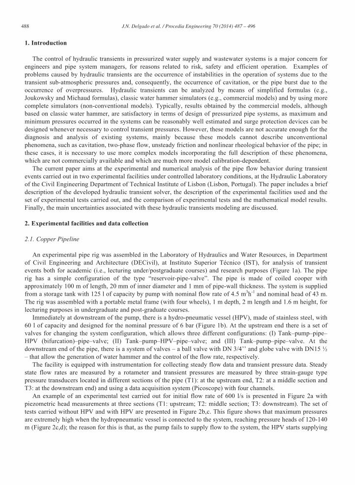
An example of an experimental test carried out for initial flow rate of 600 l/s is presented in Figure 2a with piezometric head measurements at three sections (T1: upstream; T2: middle section; T3: downstream). The set of tests carried without HPV and with HPV are presented in Figure 2b,c. This figure shows that maximum pressures are extremely high when the hydropneumatic vessel is connected to the system, reaching pressure heads of 120-140 m (Figure 2c,d); the reason for this is that, as the pump fails to supply flow to the system, the HPV starts supplying


the pipeline at downstream as well as the pipe for upstream, between the vessel and the pump; because the check valve does not instantaneously close, allowing some reverse flow, when it actually closes, the reverse flow is quite high, inducing an extremely high upsurge (see detail in Figure 2d). This shows that, under certain circumstances, surges protection devices can create higher pressures than when they are not installed in the system.

(a) (b)

Figure 1. View of the experimental copper pipe rig.

(a) (b)

(c) (d)

Figure 2. Tests carried out in the copper pipe system: (a) test without HPV for Q= 600 l/h; (b) measured piezometric heads at immediately downstream the pump without HPV for different initial flow rates; and (c), (d) measured piezometric heads with HPV, for different initial flow rates.

2.2. Steel Pipeline

A new experimental reversible pumping system was assembled at the Hydraulics Laboratory of Instituto Superior Técnico (IST), Lisbon/Portugal. The system is composed of pipeline made of steel, with a nominal

See detail (d)

CV closure 200 l/s

osure s

CV closure 400 l/s

CV closure 600 l/s


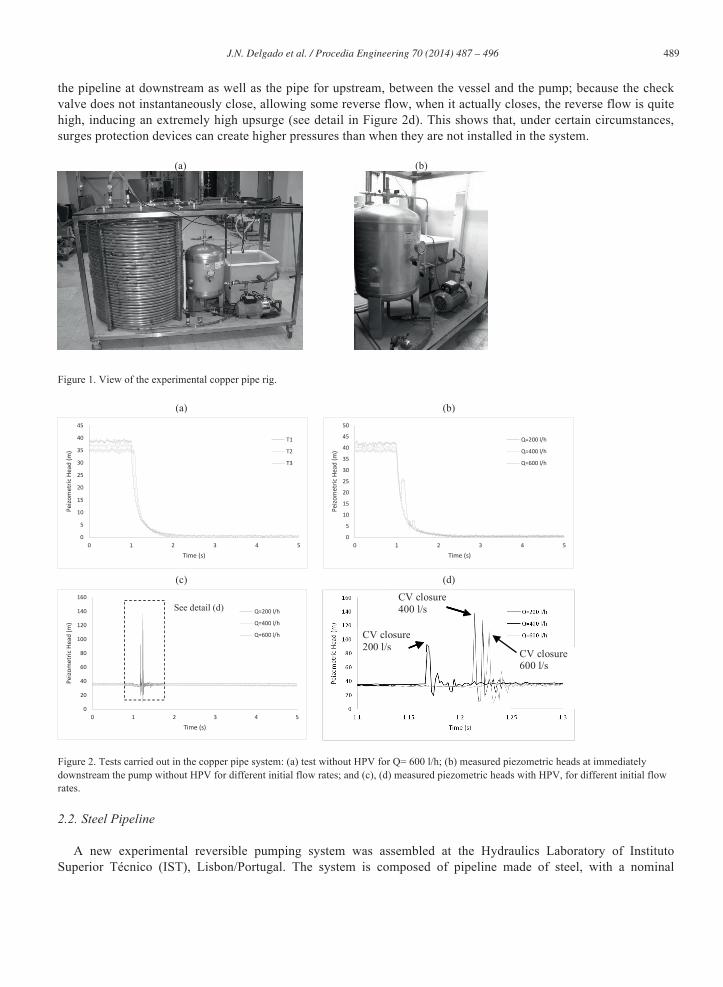
pressure of 10 bar, a total length of 115 m, an inner diameter of 206 mm and a wall thickness of 6.3 mm. The pipeline is installed along the internal perimeter of the Laboratory (Figure 3). The system is supplied from a storage tank through a centrifugal pump with a nominal flow rate of 20 l/s, a nominal elevation of 38 m and a installed power of 15 kW, with a swing check valve located at immediately downstream. A 1 m3 hydropneumatic vessel is installed at downstream the pump; this device can be connected in-line, as a side element connected through a branch or totally disconnected from the system by the opening/closing of a set of gate valves (Figure 3). The flow can circulate in the pipeline in two directions, reason why it is called a reversible system. At the downstream end there are two ball valves with 50 mm diameter each, used to generate water hammer.

Figure 3. Experimental reversible pumping system.

(a)

(b)

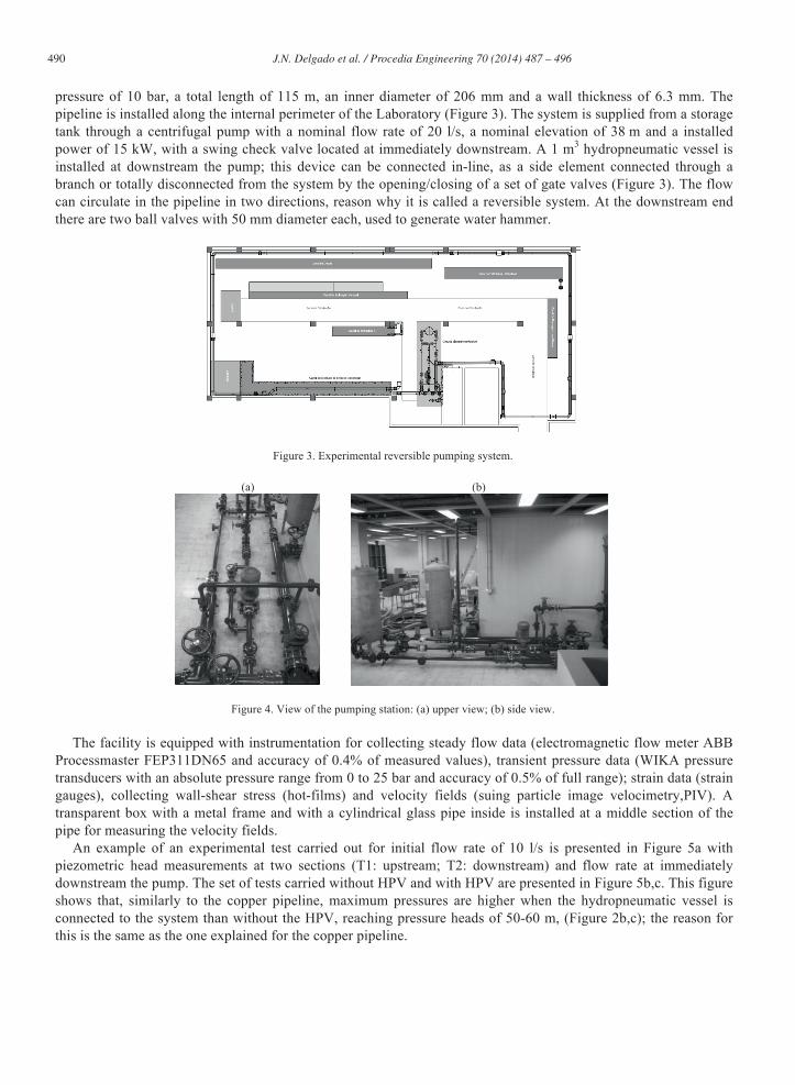
Figure 4. View of the pumping station: (a) upper view; (b) side view.

The facility is equipped with instrumentation for collecting steady flow data (electromagnetic flow meter ABB Processmaster FEP311DN65 and accuracy of 0.4% of measured values), transient pressure data (WIKA pressure transducers with an absolute pressure range from 0 to 25 bar and accuracy of 0.5% of full range); strain data (strain gauges), collecting wall-shear stress (hot-films) and velocity fields (suing particle image velocimetry,PIV). A transparent box with a metal frame and with a cylindrical glass pipe inside is installed at a middle section of the pipe for measuring the velocity fields.

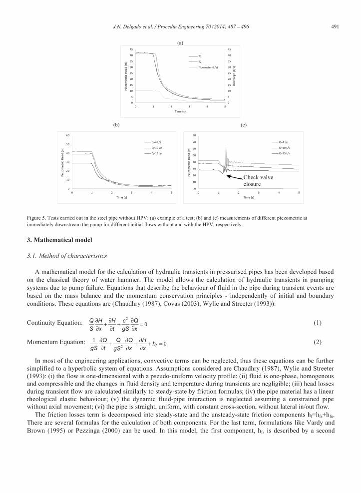
An example of an experimental test carried out for initial flow rate of 10 l/s is presented in Figure 5a with piezometric head measurements at two sections (T1: upstream; T2: downstream) and flow rate at immediately downstream the pump. The set of tests carried without HPV and with HPV are presented in Figure 5b,c. This figure shows that, similarly to the copper pipeline, maximum pressures are higher when the hydropneumatic vessel is connected to the system than without the HPV, reaching pressure heads of 50-60 m, (Figure 2b,c); the reason for this is the same as the one explained for the copper pipeline.


(a)

(b) (c)

Figure 5. Tests carried out in the steel pipe without HPV: (a) example of a test; (b) and (c) measurements of different piezometric at immediately downstream the pump for different initial flows without and with the HPV, respectively.

3. Mathematical model

3.1. Method of characteristics

A mathematical model for the calculation of hydraulic transients in pressurised pipes has been developed based on the classical theory of water hammer. The model allows the calculation of hydraulic transients in pumping systems due to pump failure. Equations that describe the behaviour of fluid in the pipe during transient events are based on the mass balance and the momentum conservation principles - independently of initial and boundary conditions. These equations are (Chaudhry (1987), Covas (2003), Wylie and Streeter (1993)):

Continuity Equation: 2

0∂ ∂ ∂+ + =∂ ∂ ∂

Q H H c QS x t gS x

(1)

Momentum Equation: 2

1 0∂ ∂ ∂+ + + =∂ ∂ ∂ fQ Q Q H h

gS t x xgS (2)

In most of the engineering applications, convective terms can be neglected, thus these equations can be further simplified to a hyperbolic system of equations. Assumptions considered are Chaudhry (1987), Wylie and Streeter (1993): (i) the flow is one-dimensional with a pseudo-uniform velocity profile; (ii) fluid is one-phase, homogenous and compressible and the changes in fluid density and temperature during transients are negligible; (iii) head losses during transient flow are calculated similarly to steady-state by friction formulas; (iv) the pipe material has a linear rheological elastic behaviour; (v) the dynamic fluid-pipe interaction is neglected assuming a constrained pipe without axial movement; (vi) the pipe is straight, uniform, with constant cross-section, without lateral in/out flow.

The friction losses term is decomposed into steady-state and the unsteady-state friction components hf=hfs+hfu. There are several formulas for the calculation of both components. For the last term, formulations like Vardy and Brown (1995) or Pezzinga (2000) can be used. In this model, the first component, hfs is described by a second

Check valve closure


order-schemes and the last component, hfu by Vitkovsky (2000)’s formulation. Previous equations are solved by the Method of Characteristics (MOC).

3.2. Boundary condition for pump trip off

For the complete mathematical representation of a pump, the relationships between discharge, Q, rotational speed, N, pumping head, H, and net torque, T, have to be specified and they are called pump characteristics. In most engineering situations, the complete pump characteristics (flow, pumping head and torque) are not available from the manufacturer. The curves tend to have similar shapes for the same specific rotation speeds. If such data are not available, then the curves must be extended by comparison with data for other specific speeds. This is an uncertain procedure, and the results of transient studies using such data must be viewed with scepticism Wylie and Streeter (1993). For these purpose, dimensionless parameters referring to the point of best efficiency (R=rated conditions) are used as a reference Chaudhry (1987):

= = = =R R R R

Q H N Tq ; h ; n ; bQ H N T

(3)

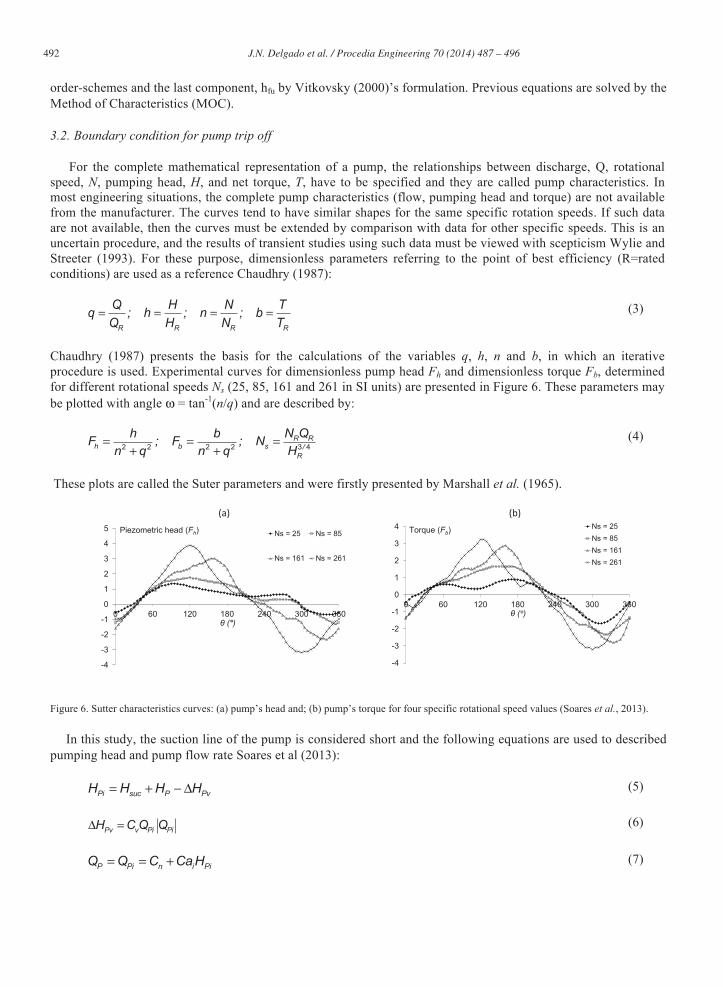
Chaudhry (1987) presents the basis for the calculations of the variables q, h, n and b, in which an iterative procedure is used. Experimental curves for dimensionless pump head Fh and dimensionless torque Fb, determined for different rotational speeds Ns (25, 85, 161 and 261 in SI units) are presented in Figure 6. These parameters may be plotted with angle ω = tan-1(n/q) and are described by:

2 2 2 2 3 4= = =+ +

R Rh b s /

R

h b N QF ; F ; Nn q n q H

(4)

These plots are called the Suter parameters and were firstly presented by Marshall et al. (1965).

Figure 6. Sutter characteristics curves: (a) pump’s head and; (b) pump’s torque for four specific rotational speed values (Soares et al., 2013).

In this study, the suction line of the pump is considered short and the following equations are used to described pumping head and pump flow rate Soares et al (2013):

= + − ΔPi suc P PvH H H H (5)

Δ =Pv v Pi PiH C Q Q (6)

= = +P Pi n i PiQ Q C CaH (7)

-4

-3

-2

-1

0

1

2

3

4

5

0 60 120 180 240 300 360

Ns = 25 Ns = 85

Ns = 161 Ns = 261

θ (°)

Piezometric head (Fh)

-4

-3

-2

-1

0

1

2

3

4

0 60 120 180 240 300 360θ (°)

Ns = 25Ns = 85Ns = 161Ns = 261

Torque (Fb)


= − − Δn B i B B BC Q CaH R tQ Q (8)

in which Hsuc = height of the liquid surface in the suction reservoir above datum, HP = pumping head, ΔHPv = head loss in the discharge valve, Cv = head loss coefficient in the valve; Cn, Ca are MOC parameters Chaudhry (1987).

3.3. Hydropneumatic Vessel

The pressurised surge tank is defined by the connection to the pipe-system and the water-level inside the tank z(t):

( )11 2 −−Δ= = + +

j j jd j j NP NPST

tH z z Q QS

(9)

⎛ ⎞= + + +⎜ ⎟⎝ ⎠j j j j

airu j fs in in NP NP

pH z h L C Q Qγ

(10)

where z = water level in the tank; Hd = piezometric head in the water surface; Hu = piezometric head at the upstream end; SST = cross section area of the tank; hfs = slope of the energy line at the inlet pipe; Lin = inlet pipe length; Cin = local head loss coefficient at the inlet pipe, C = k/2gSi

2; Si = inlet pipe cross section; k = head loss coefficient. The polytropic relationship for the perfect gas is assumed for the air inside the tank: *

0∀ =mair airp C (11)

where pair

* = absolute pressure in the air, pair*=pair+pa; ∀air = air volume; m = exponent of the polytropic gas (m=1

for the isothermal volume variation, i.e. slow transients and large air volumes; m=1.4 for the adiabatic volume variation, i.e. fast transients and small air volumes; m=1.2 in general); C0 = constant, C=pair0

* ∀air0 m, where the

subscript 0 refers to the initial conditions. The pressure and volume of air are calculated as follows:

( )1 1− −∀ =∀ − −air j air j ST j jS z z (12) *0 0= ∀ ∀ −m m

air j air air airj atmp p p (13) The air vessel is described by the previous set of equations by an iterative procedure Almeida and Koelle

(1992), Chaudhry (1987), Wylie and Streeter (1993).

4. Model calibration and testing

4.1. Copper pipeline

Pump-motor unit Inertia estimation: The pump is a centrifugal pump with the following nominal parameters: QR = 0.2 l/s, pumping head HR = 38.6 m, power PR = 1 kW, rotational speed NR = 2955 rpm, and efficiency ηR = 0.72. The pump-motor inertia was calculated by Thorley and Faithfull (1992) formulation, in which I = I1+I2, where I1 is the estimated inertia of the pump impeller and fluid, and I2 is the inertia of the motor, given by:

( )

0 96

1 30 0381000

⎛ ⎞⎜ ⎟=⎜ ⎟⎝ ⎠

.

R

R

PI .N /

( )

1 48

2 0 00431000

⎛ ⎞= ⎜ ⎟⎜ ⎟⎝ ⎠

.

R

R

PI .N /

(14)

The pump-motor inertia was estimated in I = 0.0025 kg.m2.


Wave Speed Estimation: The theoretical value of the wave speed was estimated in 1250 m/s by classic formula for a steel pipe (Young's modulus E= 177 GPa) with 20 mm inn diameter, wall thickness of 1 mm and unconstrained throughout its length. It was also estimated by the traveling time of the pressure wave between the downtream and the upstream transducer, being the obtained value 1150 m/s. This value is much lower than the theoretical value because there is gas in the liquid in a free form and cumulated along the pipeline. Pipe roughness estimation: Because the pipeline has smooth walls, steady state friction was estimated using Blasius formula White (1999).

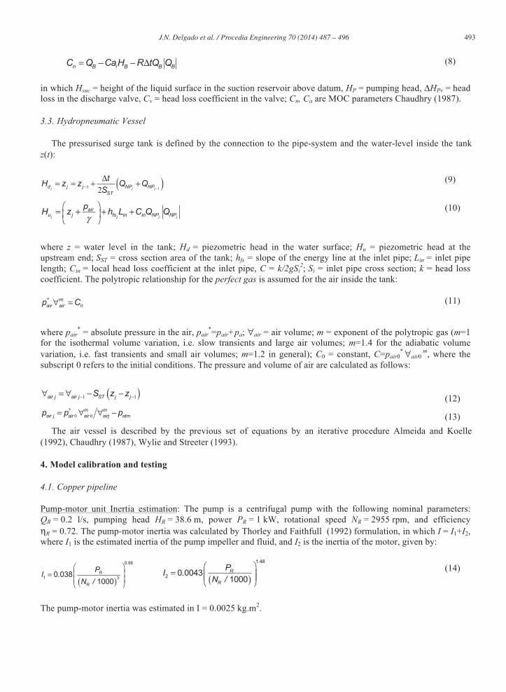
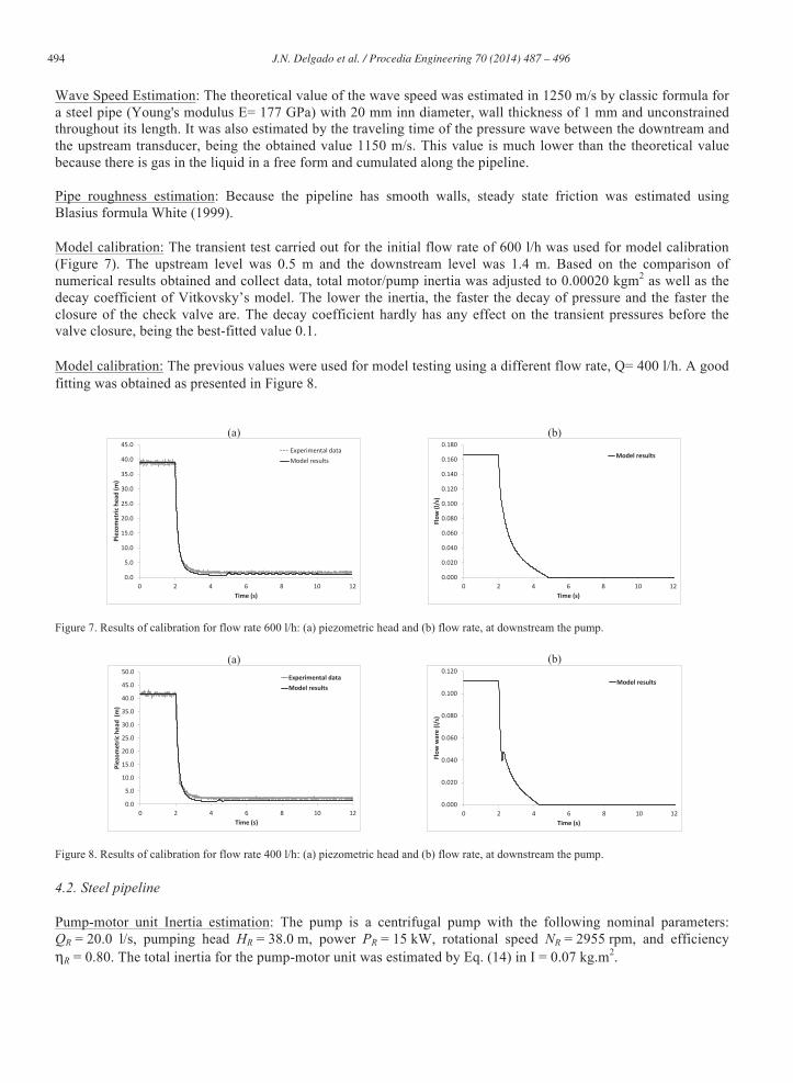
Model calibration: The transient test carried out for the initial flow rate of 600 l/h was used for model calibration (Figure 7). The upstream level was 0.5 m and the downstream level was 1.4 m. Based on the comparison of numerical results obtained and collect data, total motor/pump inertia was adjusted to 0.00020 kgm2 as well as the decay coefficient of Vitkovsky’s model. The lower the inertia, the faster the decay of pressure and the faster the closure of the check valve are. The decay coefficient hardly has any effect on the transient pressures before the valve closure, being the best-fitted value 0.1. Model calibration: The previous values were used for model testing using a different flow rate, Q= 400 l/h. A good fitting was obtained as presented in Figure 8.

(a) (b)

Figure 7. Results of calibration for flow rate 600 l/h: (a) piezometric head and (b) flow rate, at downstream the pump.

(a) (b)

Figure 8. Results of calibration for flow rate 400 l/h: (a) piezometric head and (b) flow rate, at downstream the pump.

4.2. Steel pipeline

Pump-motor unit Inertia estimation: The pump is a centrifugal pump with the following nominal parameters: QR = 20.0 l/s, pumping head HR = 38.0 m, power PR = 15 kW, rotational speed NR = 2955 rpm, and efficiency ηR = 0.80. The total inertia for the pump-motor unit was estimated by Eq. (14) in I = 0.07 kg.m2.


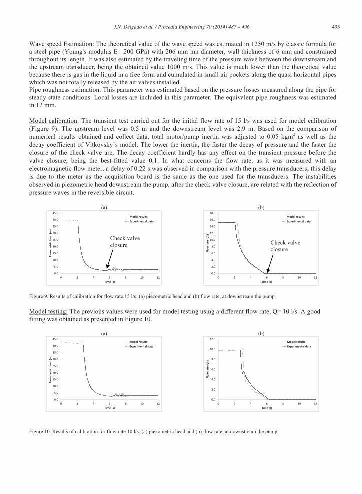
Wave speed Estimation: The theoretical value of the wave speed was estimated in 1250 m/s by classic formula for a steel pipe (Young's modulus E= 200 GPa) with 206 mm inn diameter, wall thickness of 6 mm and constrained throughout its length. It was also estimated by the traveling time of the pressure wave between the downstream and the upstream transducer, being the obtained value 1000 m/s. This value is much lower than the theoretical value because there is gas in the liquid in a free form and cumulated in small air pockets along the quasi horizontal pipes which was not totally released by the air valves installed. Pipe roughness estimation: This parameter was estimated based on the pressure losses measured along the pipe for steady state conditions. Local losses are included in this parameter. The equivalent pipe roughness was estimated in 12 mm. Model calibration: The transient test carried out for the initial flow rate of 15 l/s was used for model calibration (Figure 9). The upstream level was 0.5 m and the downstream level was 2.9 m. Based on the comparison of numerical results obtained and collect data, total motor/pump inertia was adjusted to 0.05 kgm2 as well as the decay coefficient of Vitkovsky’s model. The lower the inertia, the faster the decay of pressure and the faster the closure of the check valve are. The decay coefficient hardly has any effect on the transient pressure before the valve closure, being the best-fitted value 0.1. In what concerns the flow rate, as it was measured with an electromagnetic flow meter, a delay of 0.22 s was observed in comparison with the pressure transducers; this delay is due to the meter as the acquisition board is the same as the one used for the transducers. The instabilities observed in piezometric head downstream the pump, after the check valve closure, are related with the reflection of pressure waves in the reversible circuit.

(a) (b)

Figure 9. Results of calibration for flow rate 15 l/s: (a) piezometric head and (b) flow rate, at downstream the pump.

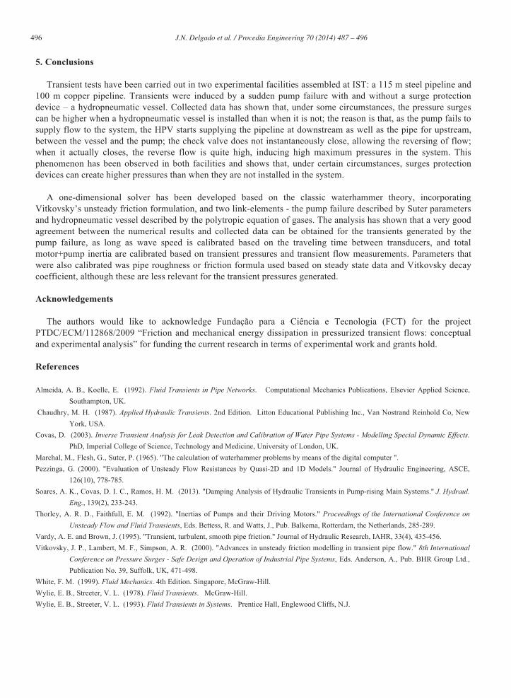
Model testing: The previous values were used for model testing using a different flow rate, Q= 10 l/s. A good fitting was obtained as presented in Figure 10.

(a) (b)

Figure 10. Results of calibration for flow rate 10 l/s: (a) piezometric head and (b) flow rate, at downstream the pump.

Check valve closure

Check valve closure


5. Conclusions

Transient tests have been carried out in two experimental facilities assembled at IST: a 115 m steel pipeline and 100 m copper pipeline. Transients were induced by a sudden pump failure with and without a surge protection device – a hydropneumatic vessel. Collected data has shown that, under some circumstances, the pressure surges can be higher when a hydropneumatic vessel is installed than when it is not; the reason is that, as the pump fails to supply flow to the system, the HPV starts supplying the pipeline at downstream as well as the pipe for upstream, between the vessel and the pump; the check valve does not instantaneously close, allowing the reversing of flow; when it actually closes, the reverse flow is quite high, inducing high maximum pressures in the system. This phenomenon has been observed in both facilities and shows that, under certain circumstances, surges protection devices can create higher pressures than when they are not installed in the system.

A one-dimensional solver has been developed based on the classic waterhammer theory, incorporating

Vitkovsky’s unsteady friction formulation, and two link-elements - the pump failure described by Suter parameters and hydropneumatic vessel described by the polytropic equation of gases. The analysis has shown that a very good agreement between the numerical results and collected data can be obtained for the transients generated by the pump failure, as long as wave speed is calibrated based on the traveling time between transducers, and total motor+pump inertia are calibrated based on transient pressures and transient flow measurements. Parameters that were also calibrated was pipe roughness or friction formula used based on steady state data and Vitkovsky decay coefficient, although these are less relevant for the transient pressures generated.

Acknowledgements

The authors would like to acknowledge Fundação para a Ciência e Tecnologia (FCT) for the project PTDC/ECM/112868/2009 “Friction and mechanical energy dissipation in pressurized transient flows: conceptual and experimental analysis” for funding the current research in terms of experimental work and grants hold.

References

Almeida, A. B., Koelle, E. (1992). Fluid Transients in Pipe Networks. Computational Mechanics Publications, Elsevier Applied Science, Southampton, UK.

Chaudhry, M. H. (1987). Applied Hydraulic Transients. 2nd Edition. Litton Educational Publishing Inc., Van Nostrand Reinhold Co, New York, USA.

Covas, D. (2003). Inverse Transient Analysis for Leak Detection and Calibration of Water Pipe Systems - Modelling Special Dynamic Effects. PhD, Imperial College of Science, Technology and Medicine, University of London, UK.

Marchal, M., Flesh, G., Suter, P. (1965). "The calculation of waterhammer problems by means of the digital computer ". Pezzinga, G. (2000). "Evaluation of Unsteady Flow Resistances by Quasi-2D and 1D Models." Journal of Hydraulic Engineering, ASCE,

126(10), 778-785. Soares, A. K., Covas, D. I. C., Ramos, H. M. (2013). "Damping Analysis of Hydraulic Transients in Pump-rising Main Systems." J. Hydraul.

Eng., 139(2), 233-243. Thorley, A. R. D., Faithfull, E. M. (1992). "Inertias of Pumps and their Driving Motors." Proceedings of the International Conference on

Unsteady Flow and Fluid Transients, Eds. Bettess, R. and Watts, J., Pub. Balkema, Rotterdam, the Netherlands, 285-289. Vardy, A. E. and Brown, J. (1995). "Transient, turbulent, smooth pipe friction." Journal of Hydraulic Research, IAHR, 33(4), 435-456. Vitkovsky, J. P., Lambert, M. F., Simpson, A. R. (2000). "Advances in unsteady friction modelling in transient pipe flow." 8th International

Conference on Pressure Surges - Safe Design and Operation of Industrial Pipe Systems, Eds. Anderson, A., Pub. BHR Group Ltd., Publication No. 39, Suffolk, UK, 471-498.

White, F. M. (1999). Fluid Mechanics. 4th Edition. Singapore, McGraw-Hill. Wylie, E. B., Streeter, V. L. (1978). Fluid Transients. McGraw-Hill. Wylie, E. B., Streeter, V. L. (1993). Fluid Transients in Systems. Prentice Hall, Englewood Cliffs, N.J.

uncertainties in hydraulic transient modelling in raising pipe systems: laboratory case studies

Documents