uncertainties in atmospheric emission projections · 1 uncertainties in atmospheric emission...

1

Uncertainties in atmospheric emission projections

Julio Lumbreras*, Rafael Borge, Javier Pérez, Encarnación Rodríguez

Laboratory of Environmental Modeling. Technical University of Madrid (UPM)

C/ José Gutiérrez Abascal, 2. 28006- Madrid. * Corresponding author: [email protected]

ABSTRACT

Emission projections are important for environmental policy, both to evaluate the

effectiveness of abatement strategies and to determine legislation compliance in the future.

Moreover, including uncertainty is an essential added value for decision makers. In this work,

projection values and their associated uncertainty are computed for emissions (both air pollutants and

greenhouse gases) in Spain following two different approaches.

The first one consists of the application of advanced statistical techniques to the most

significant activities in terms of emissions. Uncertainty bands have been derived for the Business As

Usual (or without measures) scenario through autoregressive integrated moving average (ARIMA)

models. As for the baseline scenario resampling techniques (bootstrap) were applied as an additional

nonparametric tool, which does not rely on distributional assumptions and is thus more general.

The second approach is based on a sensitivity analysis of emission projections to key inputs

on a sectoral basis (both activity rate and emission factor-related parameters). Results from the

baseline (or with measures) scenario have been compared with re-computed emission trends in a low

economic growth perspective, providing a good test of the method.

INTRODUCTION

The development of effective environmental policies is needed in order to meet regulatory

standards, international legislation and agreements in the future. The design, assessment and

comparison of control strategies require the support of an integrated modeling system. The Technical

University of Madrid (UPM) is currently developing and implementing such a modeling system for

Spain. The system is based on three major components, which should be considered as a work in

progress, since they are currently being upgraded and improved. These components are as follows:

1) Spain’s Emission Projections (SEP)1 model as a result of the application of the Consistent

Emission Projection (CEP) model to Spain2. Emissions for the main atmospheric pollutants

and greenhouse gases are available up to 2020. These emissions are based on individual,

highly-detailed projections for nearly 300 emission categories according to the Selected

Nomenclature for Air Pollution (SNAP) classification. National figures are obtained through

an integration methodology that guarantee full consistency among individual projections and

complete agreement with the National Atmospheric Emission Inventory (SNAEI)3 estimates

for past years. A piece of software called EmiPro1 has been developed to implement the

SEP’s methods and support the QA/QC process in emission projections. This tool also assists

2

report generation, including mapping to other nomenclatures relevant in the framework of the

Clean Air For Europe (CAFE) program and comparison with other European models

(RAINS, PRIMES, etc.)

2) An air quality modeling system for the Iberian Peninsula based on WRF, SMOKE and

CMAQ models. It includes the adaptation of the SMOKE system to European conditions and

the integration of the SNAEI and SEP’s databases as inputs to the emission preparation for

modeling process.

3) Impact-oriented modules. Complementary to the regulatory view of air pollution, the system

includes a series of ancillary modules to evaluate the impact of air pollution on human health

and ecosystems in a consistent way.

This paper is focused on the first component and specifically on the development of different

methods to estimate emission projection uncertainties. As many experts expose, these uncertainties

are inevitable4. Moreover, they play a major role in environmental decision-making as atmospheric

emission estimates from all sectors must be accompanied by uncertainty estimations5. However, due

to the complexity of emission projection systems, an appropriate treatment of uncertainties is far

from trivial6. Most of worldwide emission projections include a sensitivity analysis as a first step to

show possible uncertainties. This approach is useful to identify the main parameters that influence

model results. Nevertheless, it does not permit to obtain uncertainty bands to help decision making.

The aim of this paper is to present several methods to obtain these bands.

The first approach is applicable to scenarios based on past trends that show how emissions

would grow in the absence of any technical or non-technical control measure implemented, adopted

or planned after the base year. This scenario is called “without measures” or “business as usual”. The

method relies on the ARIMA time series modeling7

as presented in Lumbreras et al. (2009)8. This

modeling assumes that the value of the series for a given time point is a linear combination of

previous values (lags) with decreasing weights and a constant conditional variance. The linear

behavior results from the assumption of multivariate normality for the joint distribution of the series.

The ARIMA methodology has been applied for decades with great success (especially on air quality

forecasting9, 10

), although other models that allow, for example, for conditional heteroscedasticity11, 12

have been derived later.

The second approach8 uses a non-parametric technique called bootstrap that was developed

by Efron13

. It is used for building forecast intervals in a “with measures” scenario (i.e. including

implemented policies and measures for reducing emissions through technology improvements and

dissemination, demand-side efficiency gains, more efficient regulatory procedures, and shifts to

cleaner fuels). In this case, the intervals are derived from the original projections including the past

(inventory) values.

The third method has been developed by the authors to use sensitivity analysis as a source of

information to derive uncertainty bands. This methodology simplifies uncertainty assessment and

3

allows other teams/regions to take advantage of their sensitivity analyses (rather than uncertainty

computation).

Uncertainty computations value integrated assessment modeling because they:

• Allow a more accurate estimation of commitments compliance in future years (such as

Kyoto Protocol or EU Directives)

• Offer a wider range of future emissions usable for negotiations

• Include uncertainty estimations of the effect of policies and measures to reduce

emissions

METHODOLOGY

ARIMA method applied to “without measures” scenarios (WoM)

The analysis is done for each pollutant at activity level (i.e. the third hierarchical level of the

EU Selected Nomenclature for Air Pollution – SNAP) applying univariate time series analysis8.

These models are capable of explaining the structure and predicting the evolution of a variable which

is observed over time. It is assumed that data are available for regular time intervals, in such way that

the inertia of the series is used for projecting.

The integrated autoregressive moving-average process of orders p and q, which is referred to

as the ARIMA (p,d,q) process, is a process defined by equation (1):

(1-B)d(1 - Ф1B - Ф2 B

2 - Ф3 B

3 - … - Фp B

p)zt = (1 - θ1B - θ2B

2 - … - θq B

q) at, (1)

where B is the backshift operator such that Byt=yt-1, the roots of Φ(B)=(1-Φ1B…)=0 are on or

outside the unit circle, and the roots of θ(B)=(1-θ1B…) are outside the unit circle and at are the

innovations which are serially uncorrelated; p is the order of the autoregressive component; q is the

order of the moving average component and d is the order of the integration.

To project emissions for WoM scenario using this method, the model of emissions should be

obtained. To do this, in a first step, the series were transformed to achieve stationarity in mean and

variance. After this, parameter estimation was done by means of maximum likelihood. Subsequently,

the hypotheses of the model must be validated. The hypotheses assumed on the errors are:

1) Zero mean

2) Constant variance

3) Uncorrelated for all lags

4) Normally distributed

Additionally, diagnosis should include the detection of any deterministic terms, whenever

present. If the hypotheses are validated, the model could be used to forecast, otherwise the model

must be redefined.

4

Finally, forecasts are obtained from the estimated model assuming that the parameter

estimates in eq. 1 are the true values. Thus, the uncertainty intervals are computed assuming that the

parameters are known, only taking into account the uncertainty of future innovations (i.e. at in eq. 1).

Bootstrap method applied to “with measures” scenarios (WM)

Other techniques (resampling, i.e. bootstrap) have been applied to compute the uncertainty

associated to the WM scenario emission projections8.

They consist of the evaluation of statistics through resampling or subsampling of the original

data (i.e. WM scenario2). The most popular resampling techniques in the literature are the

jackknife14, 15

and the bootstrap13

. The jacknife consists of, for a sample of size n, obtaining n new

artificial samples of size n-1 by deleting in turn each of the observations and computing the n

estimates corresponding to each artificial sample; we thus obtain a sample of size n of the estimator,

which can be used to estimate variances and compute confidence intervals. The bootstrap is a more

sophisticated version of artificial sampling: given the original sample of size n, we obtain new

artificial samples by selecting at random with replacement n elements of the sample. We could

obtain nn different possible artificial samples with this procedure, in practice we are restricted to

more reasonable size e.g. 10000. A new value of the estimator can now be obtained for each of the

10000 samples and, by means of a procedure equivalent to the one applied in the jacknife, this

sample of estimator values can be used to estimate variances and compute confidence intervals.

Simplified method based on Sensitivity Analysis applied to “with measures” scenarios

As an alternative to obtain uncertainty bands for WM scenario, a method based on sensitivity

analysis has been developed. It easies the procedure since it does not need any advanced statistical

tool. However, it is not as accurate and well established as the previous option.

The method consists of six steps:

1. Selection of the most relevant sectors from the emissions point of view

2. List the key factors driving emissions for each selected sector

3. Analysis of the influence of each factor on emission both at sectoral and national level

4. Definition of the most probable range of variation for each factor based on statistical

analyses (standard deviation of values from past years) and expected evolution of

drivers in the future (GDP, population, Policies and Measures, etc.)

5. Computation of the variation effect on national total emissions using factor values

within the abovementioned ranges

6. To derivate uncertainty bands from results on a national scale

RESULTS AND DISCUSSION

WoM scenario using ARIMA method

The methodology has been applied to the 20 key emission sources in Spain for the period

5

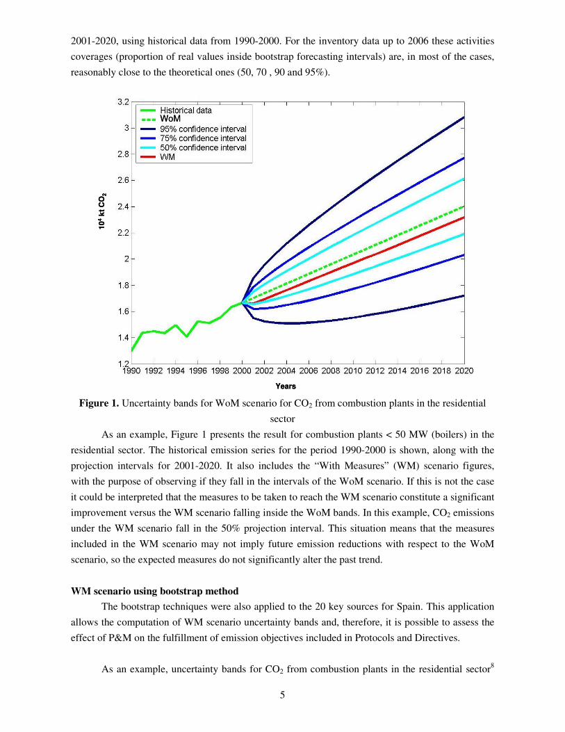
2001-2020, using historical data from 1990-2000. For the inventory data up to 2006 these activities

coverages (proportion of real values inside bootstrap forecasting intervals) are, in most of the cases,

reasonably close to the theoretical ones (50, 70 , 90 and 95%).

10

4k

tC

O2

Years

WoM

10

4k

tC

O2

Years

WoM

Figure 1. Uncertainty bands for WoM scenario for CO2 from combustion plants in the residential

sector

As an example, Figure 1 presents the result for combustion plants < 50 MW (boilers) in the

residential sector. The historical emission series for the period 1990-2000 is shown, along with the

projection intervals for 2001-2020. It also includes the “With Measures” (WM) scenario figures,

with the purpose of observing if they fall in the intervals of the WoM scenario. If this is not the case

it could be interpreted that the measures to be taken to reach the WM scenario constitute a significant

improvement versus the WM scenario falling inside the WoM bands. In this example, CO2 emissions

under the WM scenario fall in the 50% projection interval. This situation means that the measures

included in the WM scenario may not imply future emission reductions with respect to the WoM

scenario, so the expected measures do not significantly alter the past trend.

WM scenario using bootstrap method

The bootstrap techniques were also applied to the 20 key sources for Spain. This application

allows the computation of WM scenario uncertainty bands and, therefore, it is possible to assess the

effect of P&M on the fulfillment of emission objectives included in Protocols and Directives.

As an example, uncertainty bands for CO2 from combustion plants in the residential sector8

6

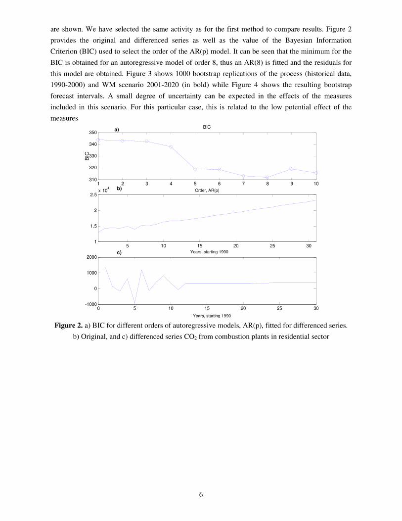
are shown. We have selected the same activity as for the first method to compare results. Figure 2

provides the original and differenced series as well as the value of the Bayesian Information

Criterion (BIC) used to select the order of the AR(p) model. It can be seen that the minimum for the

BIC is obtained for an autoregressive model of order 8, thus an AR(8) is fitted and the residuals for

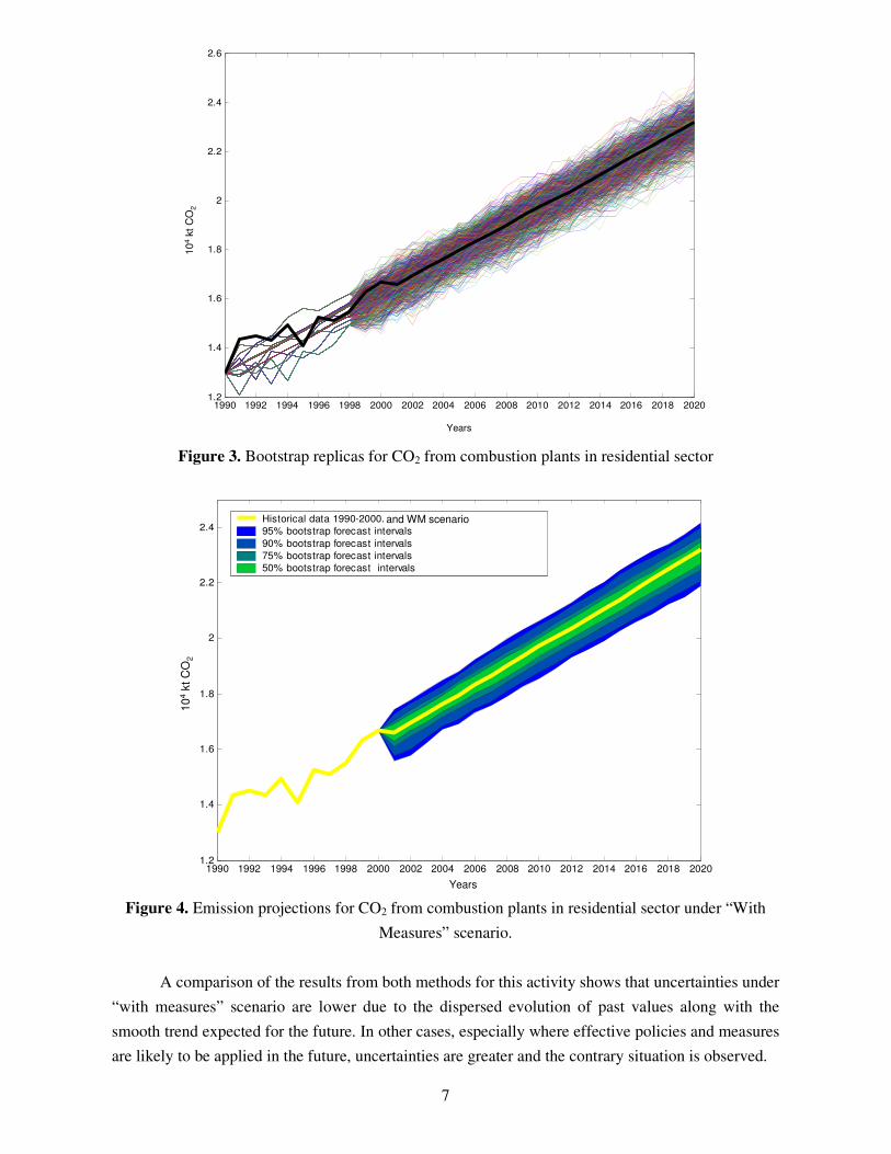
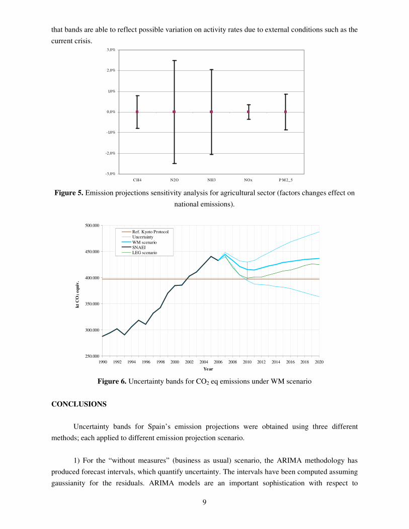
this model are obtained. Figure 3 shows 1000 bootstrap replications of the process (historical data,

1990-2000) and WM scenario 2001-2020 (in bold) while Figure 4 shows the resulting bootstrap

forecast intervals. A small degree of uncertainty can be expected in the effects of the measures

included in this scenario. For this particular case, this is related to the low potential effect of the

measures

1 2 3 4 5 6 7 8 9 10310

320

330

340

350BIC

5 10 15 20 25 301

1.5

2

2.5x 10

4 Original series

0 5 10 15 20 25 30-1000

0

1000

2000Differenced series

Order, AR(p)

BIC

a)

Years, starting 1990

Years, starting 1990

b)

c)

Figure 2. a) BIC for different orders of autoregressive models, AR(p), fitted for differenced series.

b) Original, and c) differenced series CO2 from combustion plants in residential sector

7

Years

1990 1992 1994 1996 1998 2000 2002 2004 2006 2008 2010 2012 2014 2016 2018 20201.2

1.4

1.6

1.8

2

2.2

2.4

2.6x 10

CO

2 e

mis

sio

ns

10

4kt

CO

2

Years

1990 1992 1994 1996 1998 2000 2002 2004 2006 2008 2010 2012 2014 2016 2018 20201.2

1.4

1.6

1.8

2

2.2

2.4

2.6x 10

CO

2 e

mis

sio

ns

10

4kt

CO

2

1990 1992 1994 1996 1998 2000 2002 2004 2006 2008 2010 2012 2014 2016 2018 20201.2

1.4

1.6

1.8

2

2.2

2.4

2.6x 10

CO

2 e

mis

sio

ns

1990 1992 1994 1996 1998 2000 2002 2004 2006 2008 2010 2012 2014 2016 2018 20201.2

1.4

1.6

1.8

2

2.2

2.4

2.6x 10

CO

2 e

mis

sio

ns

10

4kt

CO

2

Years

Figure 3. Bootstrap replicas for CO2 from combustion plants in residential sector

1990 1992 1994 1996 1998 2000 2002 2004 2006 2008 2010 2012 2014 2016 2018 20201.2

1.4

1.6

1.8

2

2.2

2.4

x 10

CO

2 e

mis

sio

ns

Historical data 1990-2000. Emission project, base scenario

95% bootstrap forecast intervals




10

4kt

CO

2

Years

and WM scenario

1990 1992 1994 1996 1998 2000 2002 2004 2006 2008 2010 2012 2014 2016 2018 20201.2

1.4

1.6

1.8

2

2.2

2.4

x 10

CO

2 e

mis

sio

ns






10

4kt

CO

2

Years

1990 1992 1994 1996 1998 2000 2002 2004 2006 2008 2010 2012 2014 2016 2018 20201.2

1.4

1.6

1.8

2

2.2

2.4

x 10

CO

2 e

mis

sio

ns






1990 1992 1994 1996 1998 2000 2002 2004 2006 2008 2010 2012 2014 2016 2018 20201.2

1.4

1.6

1.8

2

2.2

2.4

x 10

CO

2 e

mis

sio

ns






10

4kt

CO

2

Years

and WM scenario

Figure 4. Emission projections for CO2 from combustion plants in residential sector under “With

Measures” scenario.

A comparison of the results from both methods for this activity shows that uncertainties under

“with measures” scenario are lower due to the dispersed evolution of past values along with the

smooth trend expected for the future. In other cases, especially where effective policies and measures

are likely to be applied in the future, uncertainties are greater and the contrary situation is observed.

8

WM scenario derived from Sensitivity Analysis

Uncertainty bands for total national projections were calculated following the steps presented

in section 2. The sectors selected for Sensitivity Analysis are shown in Table 1.

Afterwards, the driving factors were identified. An analysis of their influence on emissions

was done by varying their values and calculating associated emissions. Finally, the most probable

range of variation was determined for the calculation of emission bands. Table 2 and Figure 5 show

these steps for the agricultural sector (cultures, enteric fermentation from animals, manure

management and use of pesticides and limestone).

Table 1. Sectors selection including their contribution to national emissions Sector SO2 NOx NMVOC NH3 CO2 N2O CH4 SF6 HFC PFC PM2.5

Power Plants 70,6% 19,4% 0,8% 0,0% 28,0% 1,8% 0,2% 0,0% 0,0% 0,0% 7,1%

Residential sector 1,1% 1,2% 4,0% 0,0% 5,0% 0,7% 1,5% 0,0% 0,0% 0,0% 16,3%

Combustion in industry

(except cement) 8,5% 15,3% 2,8% 0,0% 15,2% 1,6% 0,4% 0,0% 0,0% 0,0% 3,4%

Cement sector 1,5% 3,4% 0,2% 0,0% 7,9% 0,3% 0,0% 0,0% 0,0% 0,0% 0,5%

Aluminium 0,3% 0,1% 0,0% 0,0% 0,2% 0,0% 0,0% 0,0% 0,0% 55,5% 0,4%

Solvent and painting

use 0,0% 0,0% 37,3% 0,0% 0,2% 0,0% 0,0% 0,0% 0,0% 0,0% 0,0%

Refrigeration

equipments 0,0% 0,0% 0,0% 0,0% 0,0% 0,0% 0,0% 0,0% 76,1% 43,0% 0,0%

Electric equipments 0,0% 0,0% 0,0% 0,0% 0,0% 0,0% 0,0% 100,0% 0,0% 0,0% 0,0%

Road transport 0,2% 31,7% 17,5% 1,8% 26,5% 8,9% 0,4% 0,0% 0,0% 0,0% 24,6%

Rail transport 0,0% 0,25% 0,05% 0,0% 0,1% 0,1% 0,0% 0,0% 0,0% 0,0% 0,2%

Waste management 0,0% 0,1% 0,0% 1,7% 0,2% 0,2% 18,2% 0,0% 0,0% 0,0% 0,0%

Agriculture (including

livestock) 1,2% 8,7% 11,5% 94,6% 2,1% 56,9% 59,7% 0,0% 0,0% 0,0% 0,0%

TOTAL 83% 80% 74% 98% 85% 71% 81% 100% 76% 98% 52%

Table 2. Most probable range for agricultural factors

Factor Upper limit Lower limit

Agricultural surface + 4 % - 4 %

Inorganic fertilization rate +10 -10

Number of dairy cows + 4 % - 4 %

Number of other cattle + 4 % - 4 %

Number of fattening pigs + 4 % - 2 %

Number of sows + 4 % - 2 %

Number of ovine + 4 % - 4 %

Number of laying hens + 4 % - 4 %

% of urea use + 2 % - 4 %

Results are shown in Figure 6. They have been compared with re-computed emission trends

under a low economic growth situation (LEG scenario). This scenario was calculated applying also

the CEP model to Spain but considering new economic forecasts for 2009-2011 that considered the

financial and economic crisis. These forecasts provide new activity rates (electricity consumption,

industrial production, mobility, etc.) and macroeconomic values (GDP, population, prices, etc.).

Results for LEG scenario are within uncertainty bands but very close to the lower values. This shows

9

that bands are able to reflect possible variation on activity rates due to external conditions such as the

current crisis.

-3,0%

-2,0%

-1,0%

0,0%

1,0%

2,0%

3,0%

CH4 N2O NH3 NOx P M2_5

Figure 5. Emission projections sensitivity analysis for agricultural sector (factors changes effect on

national emissions).

250.000

300.000

350.000

400.000

450.000

500.000

1990 1992 1994 1996 1998 2000 2002 2004 2006 2008 2010 2012 2014 2016 2018 2020

Year

kt

CO

2 e

qu

iv.

Ref. Kyoto Protocol

Uncertainty

WM scenario

SNAEI

LEG scenario

Figure 6. Uncertainty bands for CO2 eq emissions under WM scenario

CONCLUSIONS

Uncertainty bands for Spain’s emission projections were obtained using three different

methods; each applied to different emission projection scenario.

1) For the “without measures” (business as usual) scenario, the ARIMA methodology has

produced forecast intervals, which quantify uncertainty. The intervals have been computed assuming

gaussianity for the residuals. ARIMA models are an important sophistication with respect to

10

regression models.

2) For the “with measures” (baseline) scenario, where the starting point were the annual

projected values computed by means of the CEP methodology applied to Spain, two contributions

are included in this paper:

a) the incorporation of stochastic modeling to produce forecast intervals by means of

non parametric bootstrap methods. The essential added value of non parametric

techniques is that they are not restricted to distributional assumptions, thus being of

more general application.

b) the calculation of uncertainty bands based on sensitivity analyses carried out for the

most pollutant sectors

From the application of the first method for the most important activities in Spain in terms of

emissions it was found (although not shown) that in most of the cases WM projections fall within the

WoM uncertainty bands. However, when effective policies and measures are expected for the future,

the trend has inflection points and the values of future emissions are close to the boundaries of the

bands. Intervention analysis can be applied in future research to quantify the effect of these policy

changes.

The second method allows the calculation of uncertainty bands for the scenario used to

evaluate compliance of international commitments. It provides a better estimate of future situation.

However, it would be necessary to carry out the uncertainty analyses for the total national emission

projections, i.e. for the sum of individual emissions over all activities. This raises the problem of how

uncertainties are added up, which is highly dependent on the correlation between emissions for

different activities. This would provide a means of computing the total uncertainty when evaluating

compliance.

The third method quantifies this total uncertainty in a more simple way. It has been applied

for Spanish projections showing a very good performance. Moreover, it has been compared with re-

computed emission trends in a low economic growth perspective, providing a good test of the

method. It appears as a good possibility to carry out uncertainty assessments for countries that are

currently developing sensitivity analyses.

ACKNOWLEDGEMENTS

The authors would like to thank the Environment Ministry of Spain for funding the project

and the staff from the “Dirección General de Calidad y Evaluación Ambiental” for their

collaboration.

11

REFERENCES

1- Borge, R., Lumbreras, J., Rodríguez, E., Casillas, I., 2005. Supporting Spain’s national

emission projections with the EmiPro tool. 14th Annual International Emission Inventory

Conference "Transforming Emission Inventories - Meeting Future Challenges Today". US

Environmental Protection Agency, 11-14 April 2005, Las Vegas, Nevada.

2- Lumbreras, J., Borge, R., de Andres, J.M., Rodriguez, E., 2008. A model to calculate

consistent atmospheric emission projections and its application to Spain. Atmospheric

Environment 42, 5251–5266.

3- MMA (Spanish Ministry of the Environment), 2004. CORINAIR Spain 2001 and 2002

Inventories of emissions of pollutants into the Atmosphere. Prepared by AED for the

Secretariat-General for the Environment. Directorate-General for Environmental Quality and

Assessment.

4- IPCC. 2006. IPCC Guidelines for National Greenhouse Gas Inventories, USA.

5- Kioutsioukis, I., Tarantola, S., Saltelli, A., Gatelli, D., 2004. Uncertainty and global

sensitivity analysis of road transport emission estimates. Atmospheric Environment 38,

6609–6620

6- van Sluijs, J., 1996. Integrated Assessment Models and the Management of Uncertainties.

WP-96–119. International Institute for Applied Systems Analysis (IIASA), Laxenburg,

Austria.

7- Box, G.E.P., Jenkins, G.M., 1970. Time Series Analysis Forecasting And Control. Holden-

Day, San Francisco, USA, 553 pp.

8- Lumbreras, J., García-Martos, C., Mira, J., Borge, R., 2009. Computation of uncertainty for

atmospheric emission projections from key pollutant sources in Spain. Atmospheric

Environment 43, 1557–1564.

9- Chelani, A.B., Devotta, S., 2006. Air quality forecasting using a hybrid autoregressive and

nonlinear model. Atmospheric Environment 40, 1774–1780

10- Goyal, P., Chan, A.T., Jaiswal, N., 2006. Statistical models for the prediction of respirable

suspended particulate matter in urban cities. Atmospheric Environment 40, 2068–2077.

11- Engle, R., 1982. Autoregressive conditional heteroscedasticity with estimates of variance of

United Kingdom inflation. Econometrica 50, 987–1007.

12- Bollerslev, T., 1986. Generalized autoregressive conditional heteroscedasticity. Journal of

Econometrics 31, 307–327.

13- Efron, B., 1979. Bootstrap methods: another look at the jackknife. The Annals of Statistics 7,

1–26.

14- Quenouille, M., 1949. Approximation test of correlation in time series. Journal of the Royal

Statistical Society. Series B 11, 18–84.

15- Tukey, J., 1958. Bias and confidence in not quite large samples. The Annals of Mathematical

Statistics 29, 614.

12

KEY WORDS

Integrated assessment modeling

Emission projections

Uncertainty

ARIMA models

Bootstrap

Sensitivity Analysis

uncertainties in atmospheric emission projections · 1 uncertainties in atmospheric emission...

Documents