u eatworms.swmed.edu/~leon u [email protected]
TRANSCRIPT
eatworms.swmed.edu/~leon [email protected]
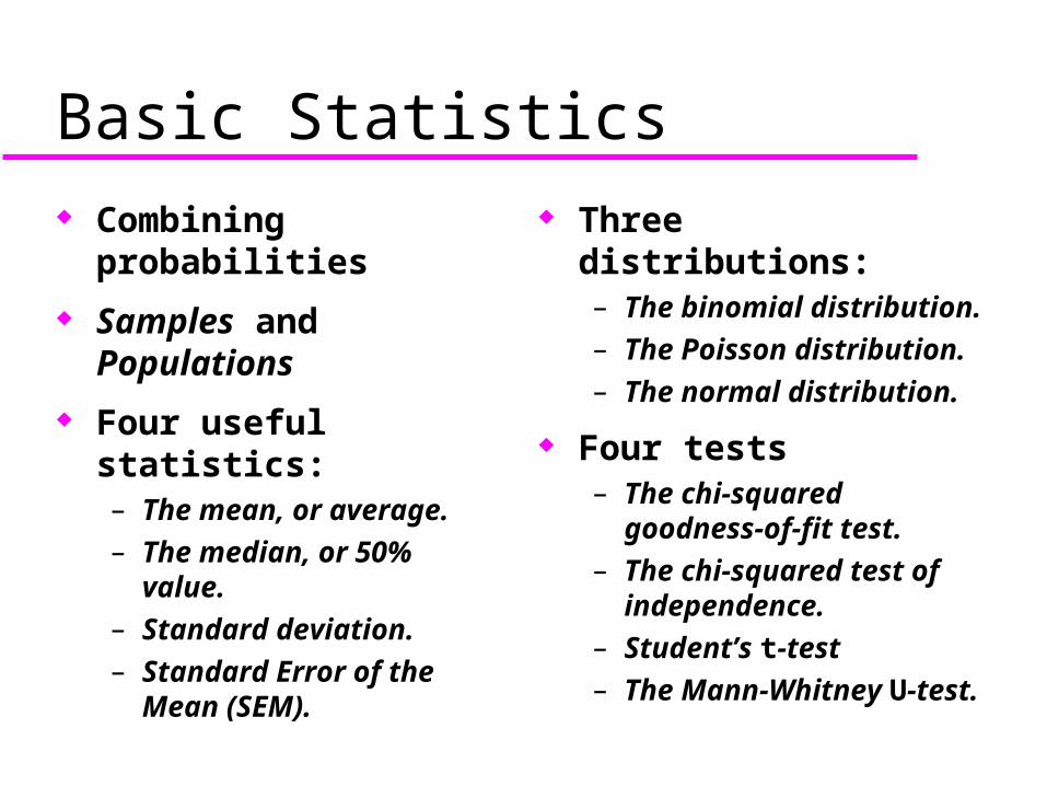
Basic Statistics Combining probabilities
Samples and Populations
Four useful statistics:– The mean, or average.– The median, or 50%
value.– Standard deviation.– Standard Error of the
Mean (SEM).
Three distributions:– The binomial distribution.– The Poisson distribution.– The normal distribution.
Four tests– The chi-squared
goodness-of-fit test.– The chi-squared test of
independence.– Student’s t-test– The Mann-Whitney U-test.
Combining probabilities
When you throw a pair of dice, what is the probability of getting 11?
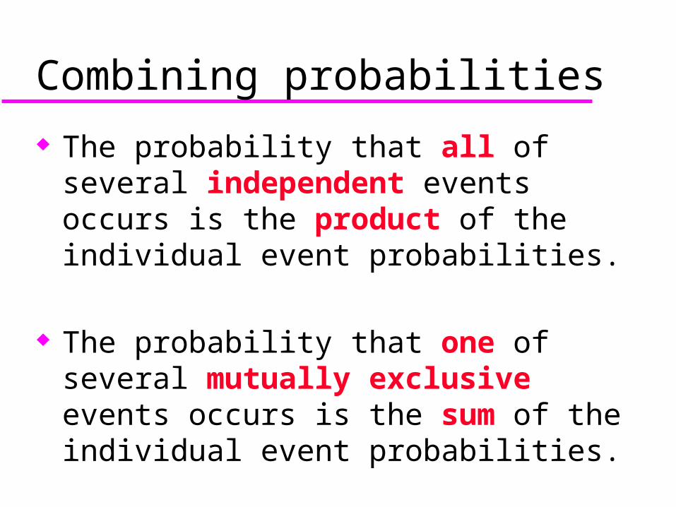
Combining probabilities
The probability that all of several independent events occurs is the product of the individual event probabilities.
The probability that one of several mutually exclusive events occurs is the sum of the individual event probabilities.
Combining probabilities
When you throw a pair of dice, what is the probability of getting 11?
When you throw five dice, what is the probability that at least one shows a 6?
Combining probabilities
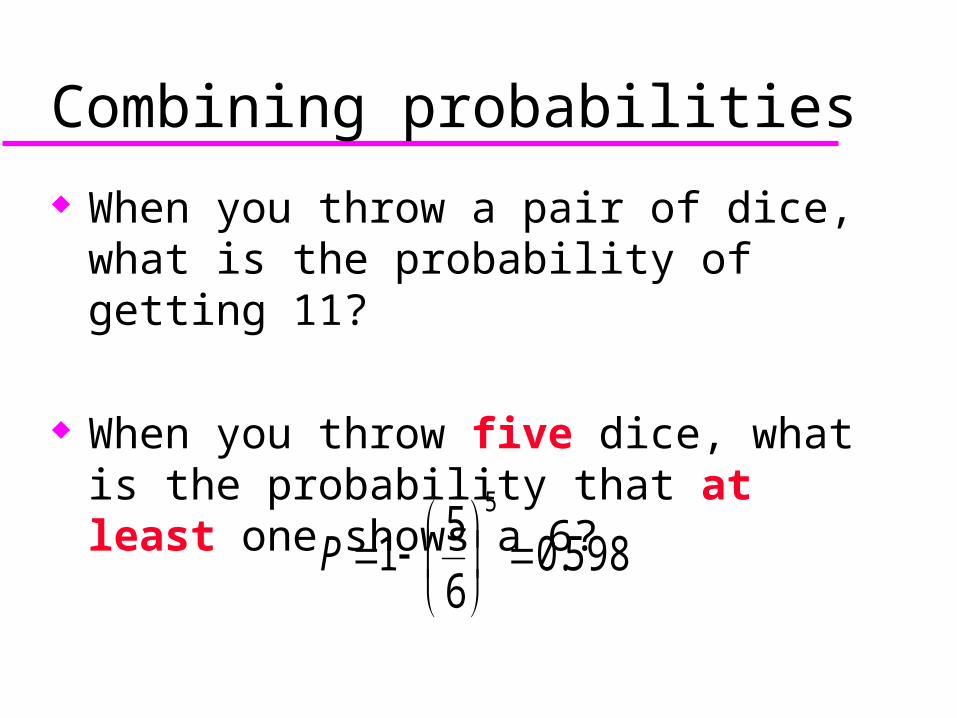
When you throw a pair of dice, what is the probability of getting 11?
When you throw five dice, what is the probability that at least one shows a 6?
598.06
51
5
P
Populations and samples
What proportion of the population is female?
Populations and samples
What proportion of the population is female?
Abstract populations: what does a mouse weigh?
Populations and samples
What proportion of the population is female?
Abstract populations: what does a mouse weigh?
Population characteristics:– Central tendency: mean, median– Dispersion: standard deviation
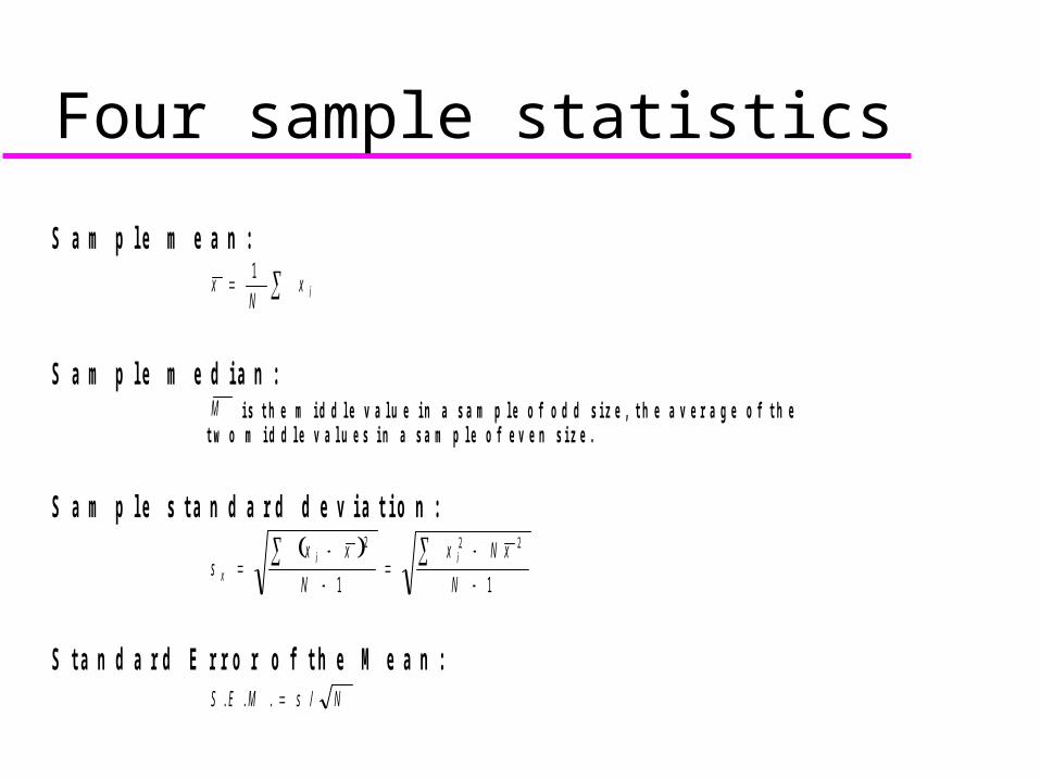
Four sample statistics
S a m p l e m e a n :
ixN
x1
S a m p l e m e d i a n :M i s t h e m i d d l e v a l u e i n a s a m p l e o f o d d s i z e , t h e a v e r a g e o f t h e
t w o m i d d l e v a l u e s i n a s a m p l e o f e v e n s i z e .
S a m p l e s t a n d a r d d e v i a t i o n :
11
222
N
xNx
N
xxs
iix
S t a n d a r d E r r o r o f t h e M e a n :NsMES /...
Standard deviation and SEM
Use standard deviation to describe how much variation there is in a population.– Example: income, if you’re interested in
how much income varies within the US population.
Use SEM to say how accurate your estimate of a population mean is.– Example: measurement of -gal activity
from a 2-hybrid test.
Sample stats: recommendations
When you report an average, report it as mean SEM.
Same for error bars in graphs. In the figure caption or the table
heading or somewhere, say explicitly that that’s what you’re reporting.
Use the median for highly skewed data.
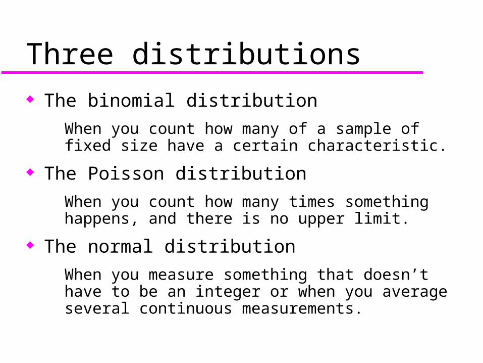
Three distributions The binomial distribution
– When you count how many of a sample of fixed size have a certain characteristic.
The Poisson distribution
– When you count how many times something happens, and there is no upper limit.
The normal distribution
– When you measure something that doesn’t have to be an integer or when you average several continuous measurements.
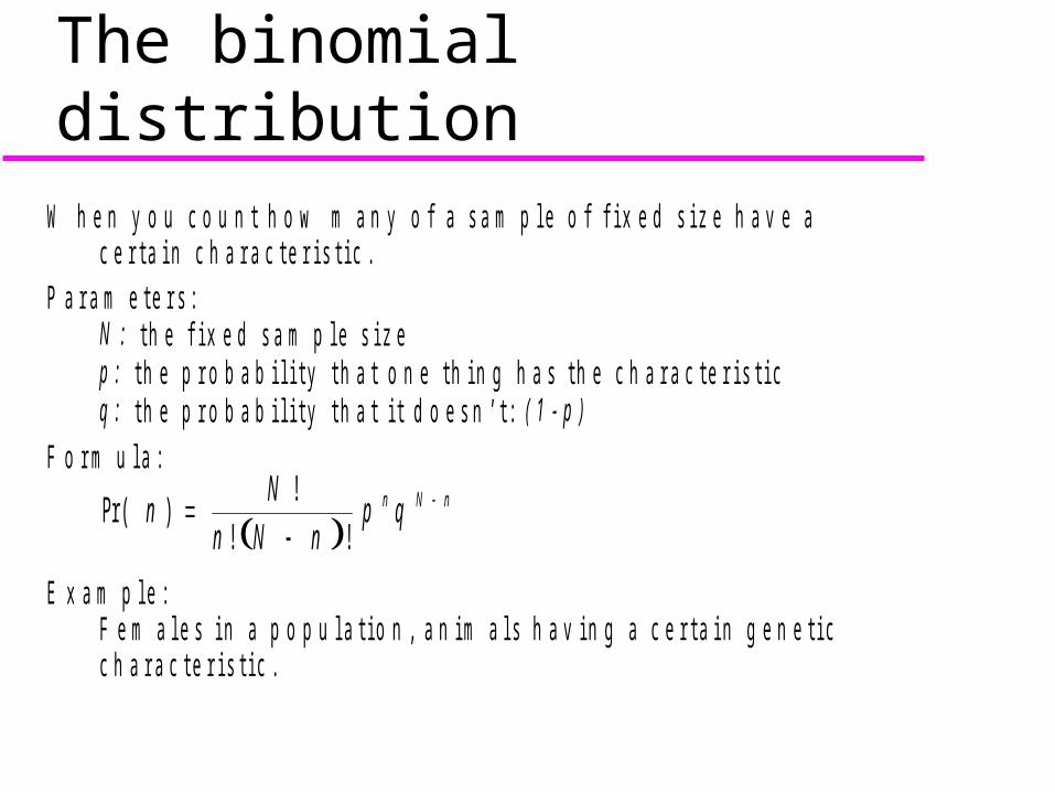
The binomial distributionW h e n y o u c o u n t h o w m a n y o f a s a m p l e o f f i x e d s i z e h a v e a
c e r t a i n c h a r a c t e r i s t i c .
P a r a m e t e r s :N : t h e f i x e d s a m p l e s i z ep : t h e p r o b a b i l i t y t h a t o n e t h i n g h a s t h e c h a r a c t e r i s t i cq : t h e p r o b a b i l i t y t h a t i t d o e s n ’ t : ( 1 - p )
F o r m u l a :
nNn qp
nNnN
n
!!!
)Pr(
E x a m p l e :F e m a l e s i n a p o p u l a t i o n , a n i m a l s h a v i n g a c e r t a i n g e n e t i cc h a r a c t e r i s t i c .
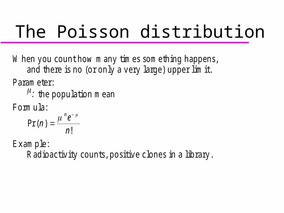
The Poisson distributionW h e n y o u c o u n t h o w m a n y tim e s so m e th in g h a p p e n s ,
a n d th e re is n o (o r o n ly a v e ry la rg e ) u p p e r lim it.P a ra m e te r:
: th e p o p u la tio n m e a n
F o rm u la :
!)Pr(
ne
nn
E x a m p le :R a d io a c tiv ity c o u n ts , p o s itiv e c lo n e s in a lib ra ry .
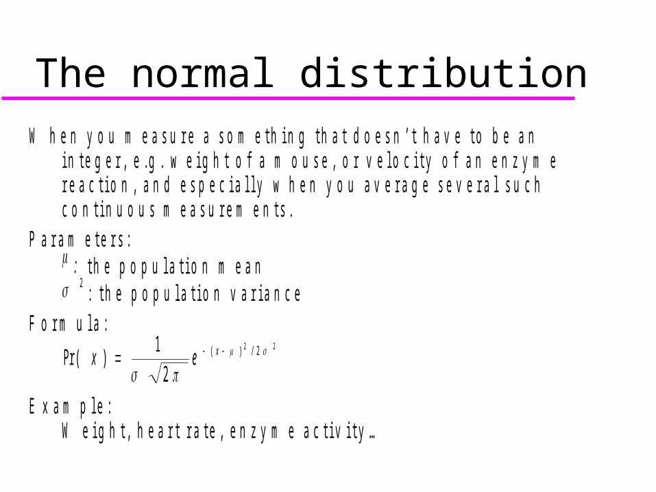
The normal distributionW h e n y o u m e a s u r e a s o m e t h i n g t h a t d o e s n ’ t h a v e t o b e a n
i n t e g e r , e . g . w e i g h t o f a m o u s e , o r v e l o c i t y o f a n e n z y m er e a c t i o n , a n d e s p e c i a l l y w h e n y o u a v e r a g e s e v e r a l s u c hc o n t i n u o u s m e a s u r e m e n t s .
P a r a m e t e r s : : t h e p o p u l a t i o n m e a n
2 : t h e p o p u l a t i o n v a r i a n c eF o r m u l a :
22 2/)(
21
)Pr(
xex
E x a m p l e :W e i g h t , h e a r t r a t e , e n z y m e a c t i v i t y …
Hypothesis testing
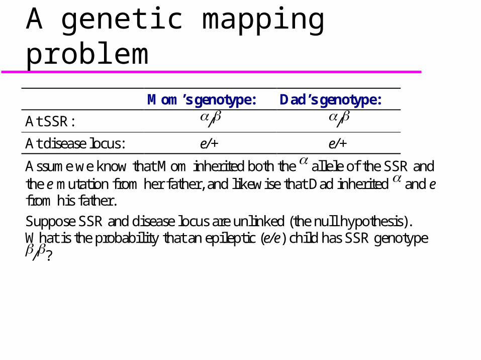
A genetic mapping problem Mom’s genotype: Dad’s genotype:
At SSR: / /
At disease locus: e/+ e/+
Assume we know that Mom inherited both the allele of the SSR and the e mutation from her father, and likewise that Dad inherited and e from his father.
Suppose SSR and disease locus are unlinked (the null hypothesis). What is the probability that an epileptic (e/e) child has SSR genotype /?
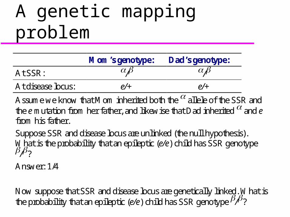
Answer: 1/4
Now suppose that SSR and disease locus are genetically linked. What is the probability that an epileptic (e/e) child has SSR genotype /?
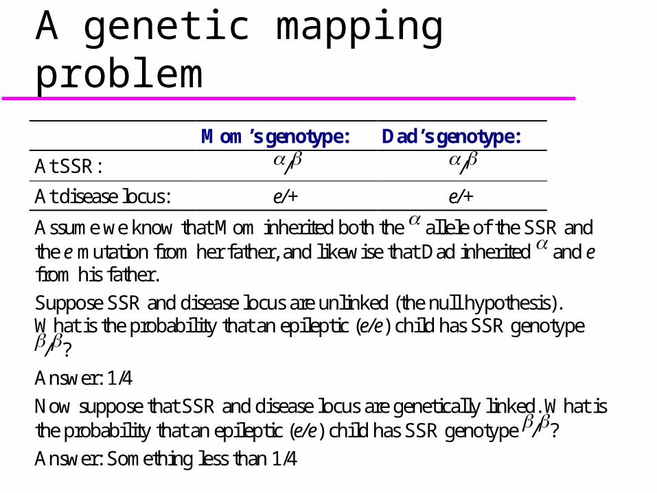
Answer: Something less than 1/4
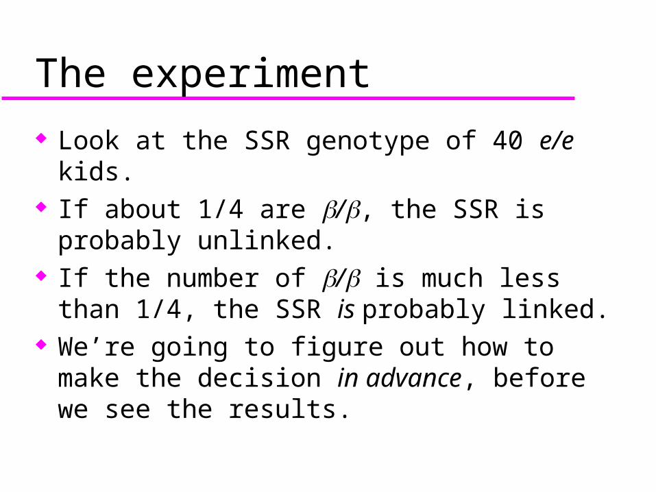
The experiment
Look at the SSR genotype of 40 e/e kids.
If about 1/4 are /, the SSR is probably unlinked.
If the number of / is much less than 1/4, the SSR is probably linked.
We’re going to figure out how to make the decision in advance, before we see the results.
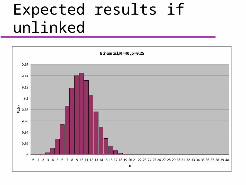
Expected results if unlinkedBinomial, N=40, p=0.25
0
0.02
0.04
0.06
0.08
0.1
0.12
0.14
0.16
0 1 2 3 4 5 6 7 8 9 10 11 12 13 14 15 16 17 18 19 20 21 22 23 24 25 26 27 28 29 30 31 32 33 34 35 36 37 38 39 40
x
Pr(
x)
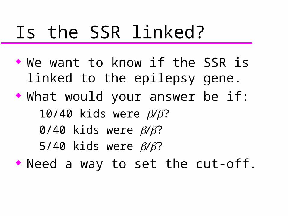
Is the SSR linked?
We want to know if the SSR is linked to the epilepsy gene.
What would your answer be if:– 10/40 kids were /?– 0/40 kids were /?– 5/40 kids were /?
Need a way to set the cut-off.
Type I errors
Suppose that in reality, the SSR and the epilepsy gene are unlinked.
Still, by chance, the number of / in our sample may be <cut-off.
We would decide incorrectly that the genes were linked.
This is a type I error.
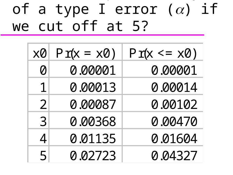
What’s the probability of a type I error () if we cut off at 5?
x0 Pr(x = x0) Pr(x <= x0)0 0.00001 0.00001 1 0.00013 0.00014 2 0.00087 0.00102 3 0.00368 0.00470 4 0.01135 0.01604 5 0.02723 0.04327
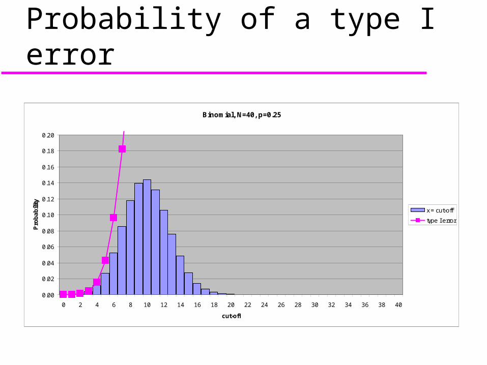
Probability of a type I error
Binomial, N=40, p=0.25
0.00
0.02
0.04
0.06
0.08
0.10
0.12
0.14
0.16
0.18
0.20
0 2 4 6 8 10 12 14 16 18 20 22 24 26 28 30 32 34 36 38 40
cut-off
Pro
ba
bili
ty
x = cut-off
type I error
Some terminology The hypothesis that nothing special is
going on is the null hypothesis, H0. A type I error is the rejection of a true
null hypothesis. The probability of a type I error is
called , or the level of significance.
Levels of significance “Statistically significant,” if nothing
more precise is added, means significant at P ≤ 5%.
“Highly significant” is less universal, but typically means P ≤ 1%.
The other level worth distinguishing isP ≤ 0.1%.
Recommendation: stick with these levels, don’t report ridiculously low probabilities.
How many tails? The test I have just described is a one-tailed
test, because we were only interested in the possibility that the frequency of / was less than ¼.
More commonly, you want to test whether an observation is either less than or greater than a predicted value.
In that case you need two cutoffs, a lower one and an upper one.
The probability of a type I error will then be the sum of the probability of too low a number and the probability of too high a number.
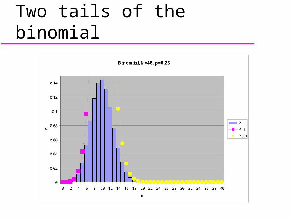
Two tails of the binomialBinomial, N=40, p=0.25
0
0.02
0.04
0.06
0.08
0.1
0.12
0.14
0 2 4 6 8 10 12 14 16 18 20 22 24 26 28 30 32 34 36 38 40
n
P
P
Pclt
Pcut
The two-tailed test Typically we put half of the
probability (2.5%) in each tail. Our decision rule will be to reject if n
≤ 4 or if n ≥ 16. This is called a two-tailed test. Recommendation: if you are at all
uncertain, do a two-tailed test.
Statistical tests Chi-squared goodness-of-fit test:
– Test whether a single measurement from a binomial matches a theoretical value.
– Test whether two Poisson distributions have equal means (by testing whether one measurement is 50% of the sum).
Chi-squared test of independence:– Test whether two binomial distributions have equal means.
Student’s t test:– Test whether two normal distributions have equal means.
Mann-Whitney U test:– Test whether two samples come from distributions with
the same location. Can be used with any continuous distribution.
Test on the probability of a binomial variable
You looked at N things (people in the room for instance), and counted the number n who matched some criterion (female, for instance).
The null hypothesis is that this is a binomial with probability p0 (some definite value that you predict based on theory).
Chi-squared goodness-of-fit test. Example: progeny classes from genetic
cross.
Tests of independence When you have measured two
binomial variates to test if the p of the two distributions is the same.
Chi-squared test of independence. For instance, suppose we want to know if the
proportion of biologists who are women is different from the proportion of doctors who are women. So we count some biologists and some doctors and we find that 24/61 biologists are women (39%), but 36/72 doctors are women (50%). We could use a chi-squared test to find out if this difference is significant. (Turns out it isn’t even close.)
Student’s t test on the means of normal variables This is when you have two sample averages
and you want to know if they’re different. For instance, maybe you have weighed mice
that are homozygous for a gene knockout and their heterozygous siblings. The hotes weigh less, a common sign that they’re unhealthy in some way, and you want to know if the difference is significant.
This test assumes that weight (or at least the average of several weights) is normally distributed.
The Mann-Whitney U test Used under almost exactly the same
circumstances as the t-test. For instance, you could use it to compare mouse weights.
Doesn’t compare averages; compares the positions of the entire distributions.
This test makes NO ASSUMPTIONS about the underlying distributions.
Probably the most useful of all statistical tests.

THINK