two-dimensional depth-averaged model simulation of...

Journal of Hydrology (2006) 327, 426–437

ava i lab le at www.sc iencedi rec t . com

journal homepage: www.elsevier .com/ locate / jhydro l

Two-dimensional depth-averaged model simulationof suspended sediment concentration distributionin a groyne field

Jennifer G. Duan a,*, S.K. Nanda b

a Division of Hydrologic Sciences, Desert Research Institute, University and Community CollegeSystem of Nevada, 755 E. Flamingo Road, Las Vegas, NV 89119, United Statesb Hydrology and Hydraulics Branch, U.S. Army Corps of Engineers, Rock Island, Illinois, United States

Received 4 November 2004; received in revised form 20 November 2005; accepted 21 November 2005

Summary River-training structures, such as spur dikes, are effective engineered methods usedto protect banks and improve aquatic habitat. This paper reports the development and applica-tion of a two-dimensional depth-averaged hydrodynamic model to simulate suspended sedimentconcentration distribution in a groyne field. The governing equations of flow hydrodynamicmodelare depth-averaged two-dimensional Reynold’s averaged momentum equations and continuityequation in which the density of sediment laden-flow varies with the concentration of suspendedsediment. The depth-averaged two-dimensional convection and diffusion equation was solved toobtain the depth-averaged suspended sediment concentration. The source term is the differencebetween suspended sediment entrainment and deposition from bed surface. One laboratoryexperiment was chosen to verify the simulated flow field around a groyne, and the other to verifythe suspended sediment concentration distribution in a meandering channel. Then, the modelutility was demonstrated in a field case study focusing on the confluence of the Kankakee and Iro-quois Rivers in Illinois, United States, to simulate the distribution of suspended sediment concen-tration around spur dikes. Results demonstrated that the depth-averaged, two-dimensionalmodel can approximately simulate the flow hydrodynamic field and concentration of suspendedsediment. Spur dikes can be used to effectively relocate suspended sediment in alluvial channels.

�c 2005 Elsevier B.V. All rights reserved.

KEYWORDSSediment transport;Numerical modeling;River confluence;River management;Hydraulic engineering

0d

5

022-1694/$ - see front matter �c 2005 Elsevier B.V. All rights reserveoi:10.1016/j.jhydrol.2005.11.055

* Corresponding author. Tel.: +1 702 862 5452; fax: +1 702 862427.E-mail address: [email protected] (J.G. Duan).

Introduction

Restorations of impaired natural channels often involve con-struction of spur dikes, which are elongated structuresextending from the bank and projecting into the flow of

d.

mailto:[email protected]

Two-dimensional depth-averaged model simulation of suspended sediment concentration distribution 427

the channel. These dikes redirect flow, protect the riverbankfrom erosion, create stable pools for aquatic habitat, andtrap suspended sediment in backwater zones. Experimentalstudies (Garde et al., 1961; Gill, 1972; Rajaratnam and Nwa-chukwu, 1983a,b; Klingeman et al., 1984; Kuhnle et al.,1999) have focused on measuring the flow field and devel-oped local scour holes around the dikes. Kuhnle et al.(1999) experimented on submerged spur dikes with overtop-ping flow, but other experimental dikes projected above thewater surface. These experiments were conducted on a mo-bile bed consisting of uniform bed material of sand or finegravel ranging from 0.2 to 2.25 mm. Suspended sedimentswere negligible, and bed-load transport was observed duringthe experiments. The distribution of suspended sedimentconcentration in a groyne field remains to be studied.

The simulation of flow and sediment transport processesaround spur dikes requires at least a two-dimensional hydro-dynamic and sediment transport model. Two-dimensionalmodels, including CCHE2D (Jia and Wang, 2001), Delft2D-Riv-ers, MIKE21C, and TAB-AMR (Langendoen, 2001), consist of atwo-dimensional hydrodynamic model and a coupled ordecoupled sediment transport model. CCHE2D, Delft2D-Riv-ers, and MIKE21C accounted for the effects of secondary cur-rents on flow momentum, mass dispersion, and sedimenttransport in curved channels. Delft2D-Rivers and MIKE21C em-ployed the modified depth-averaged momentum equationswhere momentum dispersion terms, arising from integratingthe product of the mean and secondary flow vertical profiles,are included. The dispersion terms in themass transport equa-tion resulting from the secondary flow are calculated as wellin the Delft2D-Rivers and MIKE21C models. The CCHE2D (Jiaand Wang, 2001) hydrodynamic model is based on the solutionof the depth-averaged, conventional, two-dimensionalmomentum and continuity equations. The curvature-induceddispersion terms were not included in both momentum andmass transport equations. The directions of bed-load trans-port are adjusted according to the empirical functions thatquantify the impact of secondary flow on the resultant bed-shear stress (Chiew and Parker, 1994). Both suspended andbed-load transport are simulated in these models, and non-uniform sediment transport algorithms are adopted. Althoughall are capable of handling dry and wet nodes in the computa-tional domain, the literature does not indicate their applica-tion to simulate flow and sedimentation through spur dikes.

Other two-dimensional, depth-averaged models identi-fied in the literature (Kalkwijk and de Vriend, 1980; Shimizuand Itakura, 1989; Odgaard, 1989; Yen and Ho, 1990; Mollsand Chaudhry, 1995; Ye and McCorquodale, 1997; Lienet al., 1999; Duan et al., 2001; Duan, 2004; Duan and Julien,2005) simulated flow hydrodynamics, mass dispersion, andmorphological bed processes. Secondary flow-correctionterms were included in the momentum and mass transportequations to account for the effects on distribution of flowmomentum and redirecting sediment transport. However,none of the models previously mentioned has been appliedto simulate sediment transport processes around river-train-ing structures such as spur dikes. Determining if a depth-averaged, two-dimensional model is capable of simulatingflow hydrodynamics and sediment transport through river-training structures is still an unsolved question, althoughthe depth-averaged, two-dimensional model promises tobe a cost-effective tool.

Therefore, computation of sediment transport aroundspur dikes requires further study not only for experimentalbut also computational modeling. This paper focuses onthe development and application of a depth-averaged,two-dimensional model for simulating flow field and sus-pended sediment transport around spur dikes. Detaileddescriptions and verifications of the hydrodynamic moduleare presented in an accompanying paper (Duan, 2004).

Flow simulation

Governing equations

The hydrodynamic model solves the depth-averaged Rey-nolds approximation of the Navier–Stokes equations to ob-tain depth-averaged velocities in x and y directions. Thegoverning equations for flow simulation are the depth-aver-aged Reynolds approximation of momentum equations (Eqs.(1) and (2)) and continuity equation (Eq. (3)).

oðh�uqmÞot

þ o

oxðh�u2qmÞþ

oDuu

oxþ o

oyðh�u�vqmÞþ

oDuv

oy

¼�gqmhofox� g

Dqqs

h2

2

oC

oxþ o

oxðqmhsxxÞþ

o

oyðhqmsxyÞ� sbx ð1Þ

oðh�vqmÞot

þ o

oxðh�u�vqmÞþ

oDuv

oxþ o

oyðh�v2qmÞþ

oDvv

oy

¼�gqmhofoy� g

Dqqs

h2

2

oC

oyþ o

oxðqmhsyxÞþ

o

oyðhqmsyyÞ� sby ð2Þ

o

otðhqmÞþ

o

oxh�uqm�

mtrc

ohqm

ox

� �þ o

oyðh�vqm�

mtrc

ohqm

oyÞ ¼ 0 ð3Þ

The density of sediment-laden flow (qm), a function of theconcentration of suspended sediment, is calculated as

qm ¼ q0 þDqqs

C ð4Þ

where �u and �v are depth-averaged velocity components in xand y directions, respectively; t is time; C is depth-averagedconcentration of suspended sediment that has the same unitas density, g/m3; qm, qs, and q0 are densities of sediment-laden flow, sediment particles, and clear water, respec-tively; Dq = qs � q0; f is surface elevation; h is flow depth;g is acceleration of gravity; sbx and sby are friction shearstress terms at the bottom in x and y directions, respec-tively; sxy, sxx, syx, and syy are Reynolds stress terms, whichare expressed as sxx ¼ 2mt o�u

ox, syy ¼ 2mt o�v

oy, sxy ¼ syx ¼

mt o�uoyþ o�v

ox

� �, in which mt is eddy viscosity; and Duu, Duv, and

Dvv are dispersion terms resulting from the discrepancy be-tween the depth-averaged velocity and the actual velocity,their expressions are as follows:

Duu ¼Z z0þh

z0

qmðu� �uÞ2dz

Duv ¼Z z0þh

z0

qmðu� �uÞðv � �vÞdz

Dvv ¼Z z0þh

z0

qmðv � �vÞ2dz ð5Þ

where z0 is zero velocity level. The bottom friction shearstress (sbx and sby) can be calculated as sbx ¼ Cfc�uU and

428 J.G. Duan, S.K. Nanda

sby ¼ Cfc�vU, in which U is depth-averaged total velocity,and Cfc is the Chezy’s friction coefficient corrected by con-sidering 3D effect according to Tingsanchali and Maheswa-ran (1990), and later adopted by Molinas et al. (1998) asfollows:

Cfc ¼ Cf

ffiffiffiffiffiffiffiffiffiffiffiffiffiffiffiffiffiffiffiffiffiffiffiffiffiffiffiffiffiffiffi1þ tan2ðMaa0Þ

qð6Þ

where Cf ¼ n2g

h13, in which n is Manning’s coefficient, g is grav-

itational acceleration, and h is flow depth; Ma = aw/a0; aw isthe turning angle between the bottom streamline and themain flow direction; a0 is the turning angel between themain flow and the upstream approaching flow directions.Rajaratnam and Nwachukwu (1983a,b) found that the angleaw depends on the streamline curvature and the distancefrom the groyne. Tingsanchali and Maheswaran (1990)determined when Ma equals to 2.0 the simulated hydrody-namic flow field and shear stress distribution near a groynestructure agreed with experimental measurements verywell. This study employed Eq. (6) in which the turning anglewas calculated as the ratio of depth-averaged transverseand longitudinal velocity.

In addition to the parabolic eddy viscosity turbulencemodel discussed in Duan (2004), the mixing-length modelis employed in this study for simulating more complex flowfields. The mixing-length model is used to calculate theeddy viscosity as a function of the depth-averaged mixinglength and the gradients of depth-averaged velocities inhorizontal and vertical directions

mt ¼ �l2

ffiffiffiffiffiffiffiffiffiffiffiffiffiffiffiffiffiffiffiffiffiffiffiffiffiffiffiffiffiffiffiffiffiffiffiffiffiffiffiffiffiffiffiffiffiffiffiffiffiffiffiffiffiffiffiffiffiffiffiffiffiffiffiffiffiffiffiffiffiffiffiffiffiffiffiffiffiffiffiffiffiffiffiffiffiffiffiffiffiffiffiffiffiffiffiffiffiffiffiffiffiffiffi2

o�u

ox

� �2

þ 2o�v

oy

� �2

þ o�u

oyþ o�v

ox

� �2

þ CmoU

oz

� �2��z¼h

vuut

ð7Þ

where �l is the depth-averaged mixing length; oUozis the gradi-

ent of total velocity in the vertical direction; Cm is coeffi-cient. If only horizontal velocity gradients are considered,Cm = 0, otherwise Eq. (7) yields the eddy viscosity modelwith Cm = 1.66 (Jia and Wang, 2001). The mixing length tur-bulence model adapted in this study considered the horizon-tal and vertical velocity gradients. The mixing lengthdistribution (Czernuszenko and Rylov, 2002) applied suc-cessfully in modeling three-dimensional open channel flowwas adopted, which is defined as

lðzÞh¼ 0:14� 0:08 1� z

h

� �2� 0:06 1� z

h

� �4ð8Þ

The depth-averaged mixing length can be obtained by inte-grating Eq. (8) over the flow depth,

�l ¼ 1

h

Z h

0

lðzÞdz � 0:101h ð9Þ

When considering vertical velocity gradients, the value Cm

was determined based on the condition that Eq. (7). yieldsto the parabolic eddy viscosity model when the horizontaldepth-averaged velocity gradients vanish. The mixinglength model assumes that the eddy viscosity is propor-tional to the velocity gradients in the horizontal and verti-cal directions and a ‘‘mixing length’’. Whereas theparabolic eddy viscosity turbulence model only considersshear velocity, which is related to the gradient of velocity

in the vertical direction. To simulate flow fields aroundspur dikes where flow separation and reverse occurs, themixing length model including both horizontal and verticalvelocity gradients performed better than the eddy viscos-ity model.

In contrast with the conventional depth-averagedmomentum and continuity equations, the density of sedi-ment-laden flow was considered as a temporal and spatialvariable and is a function of the concentration of suspendedsediment (Eq. (3)). The density of sediment-laden flowbeing treated as a variable is to incorporate the impact ofsediment deposition and erosion from bed surface on sus-pended sediment concentration and to couple the effectof sediment concentration on hydrodynamic flow field(Eqs. (1)–(3)). Since this study did not consider the cohesionbetween fine sediment particles, the sediment-laden flowgoverning equations are more feasible for alluvial channelscarrying non-cohesive sediment. The additional terms aris-ing from treating the density of sediment-laden flow as avariable were derived in Duan (2004).

Dispersion terms in momentum equations

Because of the secondary flow, the integration of the prod-uct of the discrepancy between the depth-averaged and theactual velocity can no longer be neglected. To derive themathematical expressions of these terms, we assumed thatthe streamwise velocity satisfies the logarithmic law writtenin the following equation:

ul

u�¼ 1

jln

z

z0

� �ð10Þ

where z is vertical coordinate, ul is velocity in the stream-wise direction, and u* is shear velocity. z0 was calculatedaccording to flow Reynolds number as follows:

z0 ¼ 0:11mu�

u�ksm6 5

z0 ¼ 0:033ksu�ksm

P 70 ð11Þ

z0 ¼ 0:11mu�þ 0:033ks 5 <

u�ksm

< 70

where ks is roughness height; and m is kinematic viscosity.Integrating the logarithmic velocity profile along the verti-cal, Eq. (10) ends up with

�ul

u�¼ 1

jz0h� 1þ ln

h

z0

� �� ð12Þ

where �ul is the depth-averaged velocity in the streamwisedirection. Combining Eqs. (10) and (12), the streamwisevelocity profile is written as

ul

�ul¼

ln zz0

� �z0h� 1þ ln h

z0

� � ð13Þ

The transverse velocity profile of the secondary flow is as-sumed to be linear. The profile of the transverse velocityproposed by Odgaard (1989) was adopted in this model.

h

Ca ha

Db Eb

Sf

Bed Load Layer

Bed Material Layer


vr ¼ �vr þ 2vsz

h� 1

2

� �ð14Þ

where vr, �vr, and vs are the transverse velocity, the depth-averaged transverse velocity, and the transverse velocity atthe water surface, respectively. Englund (1974) derived thedeviation angle of the bottom shear stress and gave that

srsl

� �b

� vr

ul

� �b

¼ 7:0h

rð15Þ

where r is the radius of channel curvature. According to Eq.(14), the secondary flow velocities at the surface and thebottom are equal. Therefore, Eq. (15) (Englund, 1974) wasused as the transverse velocity at the surface. The disper-sion terms at the streamwise and transverse directions canbe expressed as

Dcuu ¼

Z z0þh

z0

qmðul � �ulÞ2dz

Dcuv ¼

Z z0þh

z0

qmðul � �ulÞðvr � �vrÞdz

Dcvv ¼

Z z0þh

z0

qmðvr � �vrÞ2dz ð16Þ

where Dcuu;D

cuv ; and Dc

vv denote dispersion terms in curvilin-ear coordinates. Substituting Eqs. (13)–(15) into the abovedispersion terms and yields

Dcuu ¼ v2 �ul

2h½�g0 ln g0ðln g0 � 2Þ þ 2g0ð1� g0Þ� ð1� ln g0Þ � ðg0 � 1Þ3� ð17Þ

Dcuv ¼ 49:0 �ul

2 h3

r2� 1

3g30 þ

1

2g20 �

1

4g0 þ

1

12

� ð18Þ

Dcvv ¼ 3:5C �ul

2 h2

r½�g2

0 ln g0 þ g0 ln g0 � g0 þ g30� ð19Þ

where v ¼ 1g0�1�ln g0

, and g0 ¼ z0his the dimensionless zero bed

elevation. If hl denotes the angle between the streamwisedirection and the positive x-axis, and hn is the angle be-tween the transverse direction pointing to the outer bankand the positive x-axis, the depth-averaged velocities incurvilinear coordinates can be converted to that in Carte-sian coordinates according to the following equations:

�u ¼ �ul cos hl þ �vr cos hn �v ¼ �ul sin hl þ �vr sin hn ð20Þ

Then, the dispersion terms in Cartesian coordinates can becorrelated to that in curvilinear coordinates as follows:

Duu ¼ Dcuu cos

2 hl þ 2Dcuv cos hl cos hn þ Dc

vv cos2 hn ð21Þ

Dvv ¼ Dcuu sin

2 hl þ 2Dcuv sin hl sin hn þ Dc

vv sin2 hn ð22Þ

Duv ¼ Dcuu cos hl sin hl þ Dc

uvðcos hn sin hl þ sin hn cos hlÞþ Dc

vv sin hn cos hn ð23Þ

These dispersion terms were included in Eqs. (1) and (2) tosolve for flow velocity.

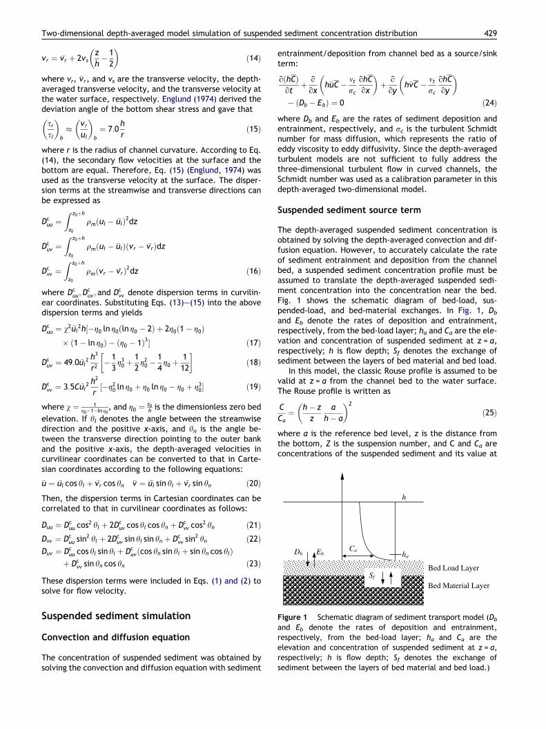
Figure 1 Schematic diagram of sediment transport model (Db

and Eb denote the rates of deposition and entrainment,respectively, from the bed-load layer; ha and Ca are theelevation and concentration of suspended sediment at z = a,respectively; h is flow depth; Sf denotes the exchange ofsediment between the layers of bed material and bed load.)

Suspended sediment simulation

Convection and diffusion equation

The concentration of suspended sediment was obtained bysolving the convection and diffusion equation with sediment

entrainment/deposition from channel bed as a source/sinkterm:

oðhCÞotþ o

oxh�uC� mt

rc

ohC

ox

� �þ o

oyh�vC� mt

rc

ohC

oy

� �

� ðDb � EbÞ ¼ 0 ð24Þ

where Db and Eb are the rates of sediment deposition andentrainment, respectively, and rc is the turbulent Schmidtnumber for mass diffusion, which represents the ratio ofeddy viscosity to eddy diffusivity. Since the depth-averagedturbulent models are not sufficient to fully address thethree-dimensional turbulent flow in curved channels, theSchmidt number was used as a calibration parameter in thisdepth-averaged two-dimensional model.

Suspended sediment source term

The depth-averaged suspended sediment concentration isobtained by solving the depth-averaged convection and dif-fusion equation. However, to accurately calculate the rateof sediment entrainment and deposition from the channelbed, a suspended sediment concentration profile must beassumed to translate the depth-averaged suspended sedi-ment concentration into the concentration near the bed.Fig. 1 shows the schematic diagram of bed-load, sus-pended-load, and bed-material exchanges. In Fig. 1, Db

and Eb denote the rates of deposition and entrainment,respectively, from the bed-load layer; ha and Ca are the ele-vation and concentration of suspended sediment at z = a,respectively; h is flow depth; Sf denotes the exchange ofsediment between the layers of bed material and bed load.

In this model, the classic Rouse profile is assumed to bevalid at z = a from the channel bed to the water surface.The Rouse profile is written as

C

Ca¼ h� z

z

a

h� a

� �Z

ð25Þ

where a is the reference bed level, z is the distance fromthe bottom, Z is the suspension number, and C and Ca areconcentrations of the suspended sediment and its value at


z = a, respectively. The actual concentration of suspendedsediment at z = a, Ca can be obtained as

Ca ¼ðCÞ

ga1�ga

� �Z R 1

ga1g � 1� �Z

dgð26Þ

where C is the depth-averaged suspended sediment concen-tration; Ca is the concentration for the suspended sedimentat the reference bed level; g is the dimensionless flowdepth; ga ¼ a

his the dimensionless reference bed level; and

Z is the suspension number. Its expression is given as

Z ¼ xe

ð27Þ

where e is the vertical mass diffusion coefficient, and x isthe fall velocity. The vertical mass diffusion relates to thefluid momentum diffusion as follows:

e ¼ b/mt ð28Þ

where mt is the turbulence eddy viscosity, and the factor bdescribes the difference in the diffusion of sediment parti-cle from the diffusion of a fluid ‘‘particle’’ and is assumedto be constant over the flow depth. b is calculated as

b ¼ 1þ 2xu�

� �2

; 0:1 <xu�< 1 ð29Þ

where u* is the shear velocity. / expresses the damping ofthe fluid turbulence by sediment particles, which is assumedto depend on the local sediment concentration

/ ¼ 1þ Ca

C�a

� �0:8

� 2Ca

C�a

� �0:4

ð30Þ

where C�a is the equilibrium suspended sediment concentra-tion at the reference bed level.

The rate of entrainment is equal to the upward flux ofsuspended sediment under equilibrium conditions. The rateof deposition is the product of falling velocity and near-bedsuspended sediment concentration. The difference betweenthe rates of entrainment and deposition from the bed-loadlayer can be calculated with the following expression.

Eb � Db ¼ axðC�a � CaÞ ð31Þ

where Db and Eb denote the rates of deposition and entrain-ment, respectively, from the bed-load layer. From an ap-praisal of existing methods to compute the referenceconcentration, Van Rijn’s formula (1984) was found to givethe best results. It follows that:

Ca ¼ 0:015d50

a

T1:5

D0:3�

ð32Þ

where D� ¼ ðs�1Þgm2

h i13is the dimensionless particle diameter;

T ¼ s� scrscr

ð33Þ

T is the dimensionless bed shear stress parameter; scr is thecritical bed shear stress according to Shield’s curve.

Boundary conditions

At the inlet, the total discharge is a constant for steady flowsimulation. The total discharge is distributed along the crosssection according to the local conveyance,

qi ¼ Kh

53i

nð34Þ

where qi is unit discharge; K is local conveyance coefficient;and n is Manning’s roughness coefficient. The current ver-sion of the model allows the specifications of roughnesscoefficient denoted as roughness height or Manning’s rough-ness coefficient for each computational node. However, forthe experimental cases selected in this paper, the roughnesscoefficient was chosen as a constant for each case based onthe bed roughness conditions described in the originalexperiments. Because the total discharge can be calculatedas the integral of unit discharge across channel width, thefollowing equation applies:

Q ¼Z

qids ¼ K

Zh

53i

nds ð35Þ

where s denotes the direction of channel width, and theflow conveyance, K, can be obtained as follows:

K ¼ Q

R h53i

nds

ð36Þ

At the outlet, surface elevation is set as a constant, which isexperimentally observed. The velocity of the outlet crosssection is calculated based on the total discharge and flowdepth at the outlet cross section.

At the sidewall, the logarithmic law is applied to the wallboundary, which is

u

ðu�Þw¼ 1

jln

y

y0

� �ð37Þ

where (u*)w is the depth-averaged shear velocity at the side-walls; y is the distance from the wall; and y0 is the locationof zero velocity near the wall. Upon obtaining the gradientof velocity, the velocity at the sidewall was calculatedbased on the velocity at the adjacent internal node. Theconcentration of suspended sediment is uniformly distrib-uted along the cross section, and set as a constant at the in-let cross sections for steady flow simulation. At the outletcross section, the gradient of suspended sediment concen-tration in the longitudinal direction equals to zero to keepbed elevation unchanged.

Model verification and application

This hydrodynamicmodelwas tested in two laboratory exper-imental cases including flow field in a groyne field and pollu-tant dispersion in meandering channels. Simulated velocitydistribution around a spur dike and velocity vector field andthe pollutant concentration field in meandering channelswere verified by laboratory experimental measurements.

Case 1: Hydrodynamic flow field in a groyne field

Experimental measurements of flow around a spur dike (Raj-aratnam and Nwachukwu, 1983a) were selected to verifythe simulation of hydrodynamic flow field. Rajaratnam andNwachukwu (1983a) conducted a series of experiments ina straight rectangular flume, which is 120 ft (37 m) long,3 ft (0.92 m) wide, and 2.5 ft (0.76 m) deep with smooth


sides and bed. A tailgate located at the downstream end ofthe flume was used to regulate flow depth during the exper-iments. Flow was measured with an 8-in. (0.2 m) magneticflow meter installed in the pipe underlying the flume. Thegroin consisted of a 3-mm-thick aluminum plate having pro-jection lengths of 3 ft (0.91 m) and 6 ft (1.83 m). The platewas high enough to project above the water surface and wasplaced within the downstream half of the flume. Flow veloc-ities were measured with a Prandtl-type pitot-static tube(3-mm external diameter) at the undisturbed uniform flowregion. In the region of skewed disturbed flow, a three-tubeyaw was used. Water surface profiles were measured with awater-level detector having an accuracy of 0.001 ft(0.3 mm). The simulated flow field was compared to anexperimental dataset for a thin 0.5-ft-long (0.15 m) alumi-num groin on a smooth bed surface with flow discharge of1.6 cfs (0.045 m3/s), flow depth of 0.62 ft (0.189 m), andFroude number of 0.19. The simulated flow field in shadedcolor was shown in Fig. 2. Velocity measurements with dis-tances of x/b = 0, 1, 2, 3 downstream of the groin werecompared with the simulated results shown in Fig. 2, inwhich the mixing-length turbulent model was adopted.Fig. 2 showed the simulated velocity distribution agreedreasonably with the experimental measurements.

Case 2: Pollutant dispersion in a meanderingchannel

Chang (1971) investigated the dispersion of pollutants inmeandering channels and measured the concentration fieldin a series of laboratory experiments. Because the second-ary flow redistributes flow momentum when passing througha channel bend, it also causes a considerable lateral mixingof pollutants so that pollutant spreading is stronger thanthat in a straight channel and thus the distribution of pollu-tants along the cross section is non-symmetric. This modelwas applied to the Case-1 experiments (Chang, 1971) to testits capability in simulating mass transport in meanderingchannels. One experimental run, in which pollutants was

Velocity (m/s)

Cha

nnel

Wid

th (

m)

0 0.5 10

0.1

0.2

0.3

0.4

0.5

0.6

0.7

0.8

0.9

Figure 2 Simulated results with the d

introduced at the mid-point of a cross section, was carriedout to study the dispersion of a pollutant, Rhodamin Bdye. The width of the flume is 2.34 m with a single meanderconsisting of two 90� bends in alternating directions con-nected by short tangents. The sinuosity of this flume set-ting, which is the ratio of actual length to the straightlength, is 1.17 (Chang, 1971), while the natural meanderingchannel usually has a sinuosity larger than 1.5 (Leopold andWolman, 1957). The cross section is rectangular with nomi-nally smooth bed and sidewalls. After the uniform flow wasestablished, velocity profiles were taken at 11 verticals foreach cross section using the pitot tube. Each velocity profilewas defined by readings taken at 9 points in the vertical, anda depth-averaged value was obtained by integration overthe flow depth. The concentration was measured by thefluorometer, which is a Turner Model 111 equipped with aspecial 5 c.c. flow through curvette manufactured by G.K.Turner Associates. Concentration was measured at four dif-ferent depths and depth-averaged value was obtained bythe integration. In the computation, bed roughness heightwas chosen as 0.001 m. The resultant friction coefficientis 0.0017–0.0018 depending on the local flow velocity. Dur-ing the experiment, flow discharge has a constant value of0.65 l/s, and the averaged flow depth is 11.5 cm. The longi-tudinal slope of the experimental flume is 0.0032.

The model was applied to the flume with a 45 · 13 mesh,which consists of 45 cross sections in the longitudinal direc-tion and 13 nodes along the transverse direction. The crosssections for the computational mesh were chosen perpen-dicular to the channel centerline. Flow discharge was con-stant at the inlet and flow depth at the outlet was set asthe experiment value of 11.5 cm for these runs. A constantconcentration of pollutant was introduced at the mid-pointof an upstream cross section.

For the dye injection at the mid-point of the channel,Fig. 3 is the plot of the velocity vector field and the watersurface elevation in shaded color. The simulated water sur-face elevation at the outer bank is much higher than that atthe inner bank. In addition, the simulated depth-averaged

1.5 2

Simulated Results

Measurements

epth-averaged mixing-length model.

Figure 3 Flow and concentration field.


velocity and concentration distribution are compared to theexperimental measurements at the second bend in Fig. 4.One finds that the simulated depth-averaged velocity agreesvery well with the measurements, which demonstrates themodel’s capability in simulating depth-averaged flow fieldin meandering channels. However, mass transport in curvedchannels has a strong three-dimensional nature because ofthe secondary flow and thus mass dispersion is much stron-ger than that in a straight channel. The mass dispersioncoefficient is much larger than the turbulent diffusion coef-ficient due to the transverse mixing of the pollutant by thesecondary flow. The Schimdt number qualifying pollutantdispersion was calibrated to achieve the desired dispersioncoefficient in the simulations. Demuren and Rodi (1986) rec-ommended the value of the Schimdt number to be 0.5 in afully three-dimensional model, with the k–e model as theturbulence closure. Ye and McCorquodale (1997) found theSchimdt number should be reduced to 0.15 in a depth-aver-

Figure 4 Comparison of simulated and measured depth-averaged velocity and concentration field.

aged model in a curvilinear collocated grid by using thedepth-averaged k–e model as the turbulence closure. Be-cause pollutant dispersion is a result of the molecular diffu-sion of the constituent and the turbulent mixing, theSchimdt number should be larger if a fully three-dimen-sional model and a sophisticated turbulent model are ap-plied. Due to the limitation of the depth-averaged modelin simulating the spiral motion of the secondary flow, theSchimdt number in this model was calibrated to achievethe results in the simulations. In the calibration, it wasfound the best results achieved with the Schimdt numberof 0.02. The comparison between simulated and measuredconcentration field using the Schimdt number, 0.02, forCase A of Chang (1971) was plotted in Fig. 4. It is obviousthat a full three-dimensional model with an accurate turbu-lence closure, such as the k–e model, is required to simu-late the helical flow pattern in meandering channels. Incase that a depth-averaged two-dimensional model is em-ployed, the Schimdt number should be significantly reduced(Ye and McCorquodale, 1997) to increase the mass diffusioncoefficient. A smaller Schimdt number is required if a sim-plified turbulence models, such as the depth-averaged mix-ing length model, is adopted. Therefore, the Schimdtnumber should be calibrated when simulating mass disper-sion in meandering channels with a depth-averaged 2D mod-el. And, the value of Schimdt number depends on theaccuracy of the hydrodynamic model and the turbulenceclosure that are employed in the model.

Case 3: Suspended sediment concentration at theconfluence of Kankakee and Iroquois rivers

Characteristics of sediment transport in the KankakeeRiverThe development model verified by experimental measure-ments was applied to study suspended sediment transportthrough proposed spurs dikes at the confluence of Kankakeeand Iroquois Rivers at Illinois. Since field measurements arenot available at the study site, this application is to illus-trate the model’s capability in solving a real engineeringproblem. The geographical location of the study site isshowed in Fig. 5. Sediment is primarily transported as sus-pended load in the Kankakee and Iroquois Rivers with higherand finer suspended loads delivered from the Iroquois River.At low flow, suspended sediment of the Kankakee River con-sists of silt and clay, while at high flow, the Kankakee River

Figure 5 Location of the study site: (a) area map and (b)study site.


transports significant quantities of fine sands. Bed load isonly 1.2% of the total suspended load, making bed loadinsignificant to the bed-evolution processes (Bhowmiket al., 1980; Bhowmik and Demissie, 2000). Because sus-pended sediment is dominant and bed material is quite finein the Kankakee River, the armoring phenomenon was notobserved at the study site. The purpose of this modelingstudy was to evaluate the impact of various alternative pro-jects on flow and sediment transport in the study reach.Flow hydrodynamic and suspended sediment concentrationfield were simulated by using the developed 2D model forthe current and two proposed conditions with dike struc-tures. The effectiveness of engineered structures, such asdikes or vanes, was then evaluated in concentrating flow to-ward the center of channel and reducing sedimentation.

Simulation of the hydrodynamic flow fieldThe model-simulated hydrodynamic flow field and concen-tration distribution of suspended sediment were studied un-der three alternative management scenarios: (1) take noaction; (2) install three short dikes; and (3) install three longdikes. Because the simulations aimed to compare results un-der these conditions, the hydrodynamic model used averageflow discharges as the simulated flow discharges: 1000 cfs(28.32 m3/s) for the Iroquois River and 2000 cfs (56.63 m3/s)for the Kankakee River. Averaged discharge, which is closeto the dominant discharge, was selected as the modelingdischarge to determine the effects of the proposed spurdike structures on fluvial geomorphology.

In addition to the constant discharge at inlets in the Kan-kakee and Iroquois Rivers, the water surface elevation atthe outlet of the Kankakee River was set at 594.77 ft(181.29 m), which was the water surface elevation at thedownstream outlet. The results of the hydrodynamic simula-tion indicated a flow velocity range of 2.0–4.0 ft/s (0.61–1.22 m/s) at the main stem of the Kankakee River whenthe discharge was 2000 cfs. The flow velocity range forthe Iroquois River with the discharge of 1000 cfs is approx-imately 1.0–2.0 ft/s (0.3–0.61 m/s). These results seemreasonable based on the observations at the Iroquois andKankakee Rivers. The concentration of suspended sedimentin the Kankakee River at Momence ranges from 10 to100 mg/l (10–100 ppm) for a discharge of 2000 cfs. The Iro-quois River at Chebanse ranges from 30 to 145 mg/l (30–145ppm) for a discharge of 1000 cfs. The sediment transportmodel for this study used mean sediment concentrations,60 mg/l (60 ppm) at Momence and 80 mg/l (80 ppm) at Che-base, as inlet boundary conditions.

The simulated concentration distribution of suspendedsediment, plotted in Fig. 6, shows two zones having very highconcentrations of suspended sediment. One zone was lo-cated at the confluence of the Kankakee and Iroquois Rivers,and the other zone was located immediately downstream ofthe island in the Kankakee River and upstream of the conflu-ence. Flow circulated in both areas, trapping suspended sed-iment. The highest modeled sediment concentration wasabout 230 mg/l (230 ppm). In contrast, sediment concentra-tion was relatively low, about 40 mg/l (40 ppm), in the Kan-kakee River upstream of the confluence where the channelwas wider. Sediment concentration moderately increasedimmediately downstream of the confluence and graduallydecreased again when the channel became wider.

To reduce the concentration of suspended sediment atthe confluence of these two rivers, the study modeled theplacement of three dikes along the left bank of the Kanka-kee River. The dikes would rise above the water surfacewhen flow discharge is 2000 cfs in the Kankakee River and1000 cfs in the Iroquois River. The computational meshwas reconstructed to make it sufficiently dense near thestructures to model the flow field near the dikes in detail.

The simulated flow field clearly showed the circulationzones downstream from the island, downstream from thedikes, and at the confluence of the two rivers. The velocitywas 3.0–4.0 ft/s in the main stem of the Kankakee Riverand about 1.0–2.0 ft/s in the Iroquois River, which was sim-ilar to the hydrodynamic modeling results obtained withoutstructures. However, the flow velocity near the dikesreached 4.0–6.0 ft/s (1.22–1.83 m/s), which could facili-tate the passage of the suspended sediment from the Iro-quois River to the Kankakee River.

Fig. 7 clearly showed that the concentration of sus-pended sediment downstream from the dikes would be veryhigh, and suspended sediment would also be high at the con-fluence and downstream from the island. Because the dis-tances between the three dikes were very short, thehighly concentrated sediment zones would not extend tothe banks. However, downstream from the third dike, thehighly concentrated sediment flow would extend furtherdownstream and finally reach the left bank of the KankakeeRiver. Compared to Fig. 6, the highest concentrations at theconfluence and downstream from the island having thethree short dikes would be slightly lower than the resultsnot having dikes. This observation indicated that the dikeswould facilitate the transport of suspended load down-stream, perhaps because the flow was constrained andvelocity was increased at the confluence. However, the con-centration of the suspended sediment downstream from theconfluence was still relatively high, about 230 mg/l.

Three longer dikes were modeled to determine if in-creased dike length would significantly constrain flow andreduce sedimentation. In this simulation, the length of thedikes was about twice as long as the dikes in Alternative#2. Because the first dike would partially block the flowfrom the Iroquois River, the height of the water surfaceon the left bank of the Iroquois River would be raised atthe confluence. Flow would be concentrated on the rightside of the Kankakee River downstream from the confluencewhere the dikes would extend almost half of the channelwidth. Besides flow velocity of 4.0–6.0 ft/s in the dike re-gion, flow velocity would remain at about 3.0–4.0 ft/s inthe main stem of the Kankakee River, while the velocityin the Iroquois River would remain at about 1.0–2.0 ft/s.

The concentration distribution of suspended sedimentfor Alternative #3 is plotted in Fig. 8. It shows that zonesof high-sediment concentrations would be located at theconfluence because the flow from the Iroquois River to themain stem of the Kankakee River would be partiallyblocked. Compared to Alternative #2, the concentration ofsuspended sediment at the confluence was higher. Eventhough increased dike length would concentrate flow down-stream from the confluence, the increased dike lengthwould result in a highly concentrated suspended sedimentzone at the confluence, which would likely result in deposi-tion at the confluence. Therefore, increasing dike length is

597.91597.649597.387597.125596.864596.602596.34596.078595.817595.555595.293595.032

Surface Elevation (ft)Q=2000 cfs

Q=1000 cfs(a)

(b)

Kankakee River

Iroquois River

6 ft/s

Island

230211.273192.545173.818155.091136.364117.63698.909180.181861.454542.727324

Concentration(g/l)Q=2000 cfs

Q=1000 cfs

Kankakee River

Iroquois River

Concentration (mg/l)

Island

Figure 6 Simulated water surface elevation, velocity vector, and suspended sediment concentration field. (a) Velocity vector andsurface elevation and (b) concentration field.


not an effective option in reducing sedimentation at theconfluence.

The hydrodynamic modeling results for Alternatives #2and #3 show that constructing dikes at the left bank of theKankakee River would definitely concentrate flow and in-crease velocity immediately downstream of the confluence.Dikes extending one-third the width of the channel would

facilitate passage of suspended sediment flowing from theIroquois River to the Kankakee River; however, if the dikelength was too long, such as in Alternative #3, the dikeswould block flow discharging from the Iroquois River to theKankakee River and potentially increase sedimentation atthe confluence. Therefore, constructing dikes or vanes toconcentrate flow is an option to reduce sedimentation, but

597.735597.487597.239596.991596.743596.495596.246595.998595.75595.502595.254595.006

Kankakee River

Q=2000 cfs

Q=1000 cfs(a)

(b)

Iroquois River

Surface Elevation (ft)

6 ft/s

Island

Dikes

230211.273192.545173.818155.091136.364117.63698.909180.181861.454542.727324

Kankakee River

Q=2000 cfs

Q=1000 cfs

Iroquois River

Concentartion(g/l)Concentration (mg/l)

Dikes

Island

Figure 7 Simulated surface elevation, velocity vector, and suspended sediment concentration distribution. (a) Velocity vector andsurface elevation and (b) concentration field.


the location, alignment, and dimension of the dikes shouldbe determined through a series of computational modelingstudy.

Summary and conclusion

The developed 2D depth-averaged numerical model distin-guishes from classical 2D model by treating the density offlow as variable changing with the concentration of sus-

pended sediment and including the bed shear stress correc-tion terms in momentum equations. Additionally, thedifference between entrainment and deposition of sus-pended sediment from bed surface was calculated as asource term in the 2D convection and diffusion equation.Experimental data from Rajaratnam and Nwachukwu(1983a) was used to verify the simulated flow field arounda spur dike. The numerical solutions of the 2D convectionand diffusion equation were verified by Chang (1971) exper-

597.736597.489597.241596.994596.746596.499596.251596.004595.756595.509595.261595.014

Surface Elevation (ft)Kankakee River

Iroquois River

Q=2000 cfs

Q=1000 cfs(a)

(b)

10 ft/s

Dikes

Island

230211.273192.545173.818155.091136.364117.63698.909180.181861.454542.727324

Kankakee River

Iroquois River

Q=2000 cfs

Q=1000 cfs

Concentration (mg/l)

Dikes

Island

Figure 8 Simulated surface elevation, velocity vector, and suspended sediment concentration distribution. (a) Velocity vector andsurface elevation and (b) concentration field.


imental data. When applying this model to a field site withmultiple proposed spur dikes, the modeling results clearlyshowed suspended sediment concentration is high at theflow separation zone downstream of the dike structure.The computational modeling results of flow hydraulics andsediment transport processes indicated that it is feasible

to use a depth-averaged, two-dimensional model to simu-late the hydrodynamic flow field and the transport of sedi-ment around spur dikes. Even though the hydrodynamicflow field around spur dikes is highly three-dimensional, thisstudy demonstrated that a depth-averaged two-dimensionalmodel is capable of reproducing flow circulation zones and


predicting the concentration of suspended sediment at theriver confluence and around spur dikes. There is no doubtthat a three-dimensional, hydrodynamic model is neededto simulate the complex flow phenomena such as separationand reverse. However, a depth-averaged, two-dimensionalmodel has advantages in being cost-effective and easy tocalibrate and in requiring less input data for practical engi-neering applications.

For the planning stage of a project, a two-dimensionalmodeling study can be used to eliminate unfavorable engi-neering plans and to assist in selecting feasible engineeringdesigns. Results from the Kankakee and Iroquois River applica-tion of the model indicated that: (1) highly concentrated sed-iment flow existed at the confluence of the rivers; (2) shortdike structures would benefit the passage of highly concen-trated sediment flow from the Iroquois River to the KankakeeRiver; and (3) longer dike structures would significantly blockflow coming from the Iroquois River and increase concentra-tion of suspended sediment at the confluence. Therefore, tofacilitate discharge of highly concentrated sediment flowfrom the Iroquois River to the Kankakee River, a sequenceof dikes could be useful. The locations, alignments, anddimensions of the dikes should be further investigated throughdetailed studies to determine cost-effective measures. A fol-low-on hydrodynamic and sediment transport modeling studyshould contribute to engineering design and confirm parame-ters of the detailed design.

Acknowledgements

This research project was sponsored by the US Departmentof Defense, Army Research Office (ARO), under Grant Num-ber DAAD19-00-1-0157. Dr. Russell Harmon is the ARO pro-gram manager. The Rock Island District (RID) of the U.S.Army Corps of Engineers also provided funding for thestudy. National Science Foundation (NSF) also provided sup-port to continue this research under Award EAR-0532691.The author is very grateful for funding provided by theabove sources and for support provided by engineers in-volved in the project. Thanks to Mr. Dong Chen, who is a re-search assistant for this project. He participated in post-processing of survey data and in generating the computa-tional meshes.

References

Bhowmik, N.G., Bonini, A., Bogner, W.C., Byrne, R.P., 1980.Hydraulics of flow and sediment transport in the Kankakee Riverin Illinois. Technical Report, Illinois State Water Survey, Cham-paign, Illinois.

Bhowmik, N.G., Demissie, M., 2000. River geometry, bankerosion, and sand bars within the main stem of the KankakeeRiver in Illinois and Indiana. Contract Report 2001–09, IllinoisState Water Survey, Watershed Science Section, Champaign,Illinois.

Chang, Y.C., 1971. Lateral mixing in meandering channels. Ph.D.thesis, University of Iowa, USA.

Chiew, Y.M., Parker, G., 1994. Incipient sediment motion on non-horizontal slopes. J. Hydraul. Res. 32 (5), 649–660.

Czernuszenko, W., Rylov, A., 2002. Modeling of three-dimensionalvelocity field in open channel flows. J. Hydraul. Res. 40 (2),135–143.

Demuren, A.O., Rodi, W., 1986. Calculation of flow and pollutantdispersion in meandering channels. J. Fluid Mech. 172, 63–92.

Duan, G., Wang, S.S.Y., Jia, Y., 2001. The applications of theenhanced CCHE2D model to study the alluvial channel migrationprocesses. J. Hydraul. Res., IAHR 39, 469–480.

Duan, J.G., 2004. Simulation of flow and mass dispersion inmeandering channels. J. Hydraul. Eng., 566–576.

Duan, J.G., Julien, P., 2005. Numerical simulation of the inceptionof meandering channel. Earth Surf. Process. Land Forms 30,1093–1110.

Englund, F., 1974. Flow and bed topography in channel bends. J.Hydraul. Eng. 100 (HY11), 1631–1648.

Garde, R.J., Subramanya, K., Nambudripad, K.D., 1961. Study ofscour around spur-dikes. J. Hydraul. Eng. 87 (HY6), 23–37.

Gill, M.A., 1972. Erosion of sand beds around spur dikes. J. Hydraul.Eng. 98 (HY9), 1587–1602.

Jia, Y., Wang, S.S.Y., 2001. ‘‘CCHE2D: two-dimensional hydrody-namic and sediment transport model for unsteady open channelflows over loose bed’’ Technical Report, NCCHE-TR-2001-1,National Center for Computational Hydroscience and Engineer-ing, University of Mississippi, University, Mississippi.

Kalkwijk, J.P.T., de Vriend, H.J., 1980. Computation of the flow inshallow river bends. J. Hydraul. Res. 18 (4), 327–342.

Klingeman, P.C., Kehe, S.M., Owusu, Y.A., 1984. Streambankerosion protection and channel scour manipulation using rockfilldikes and gabions. WRRI-98. Water Resources research Institute,Oregon State University, Corvallis, Oregon.

Kuhnle, R.A., Alonso, C.V., Shields, F.D., 1999. Geometry of scourholes associated with 90� spur dikes 125 (9), 972–978.

Langendoen, J. Eddy 2001. Evaluation of the effectiveness ofselected computer models of depth-averaged free surface flowand sediment transport to predict the effects of hydraulicstructures on river morphology. Technical Reports, NationalSedimentation Laboratory, Agricultural Research Service, USDepartment of Agriculture, Oxford, Mississippi.

Leopold, L.B., Wolman, M.G., 1957. River channel patterns:braided, meandering and straight. US Geologic Survey, Profes-sional Paper 282-B, pp. 37–86.

Lien, H.C., Hsieh, T.Y., Yang, J.C., Yeh, K.C., 1999. Bend-flowsimulation using 2D depth-averaged model. J. Hydraul. Eng. 125(10), 1097–1108.

Molinas, A., Kheireldin, K., Wu, B., 1998. Shear stress aroundvertical wall abutments. J. Hydraul. Eng. 124 (8), 822–830.

Molls, T., Chaudhry, M.H., 1995. Depth-averaged open-channel flowmodel. J. Hydraul. Eng. 12 (6), 453–465.

Odgaard, A.J., 1989. River-meander model. I: Development. J.Hydraul. Eng. 115 (11), 1433–1450.

Rajaratnam, N., Nwachukwu, B.A., 1983a. Flow near groin-likestructure. J. Hydraul. Eng., ASCE 109 (3), 463–480.

Rajaratnam, N., Nwachukwu, B.A., 1983b. Erosion near groyne-likestructures. J. Hydraul. Res., Delft, The Netherlands 21 (4), 277–287.

Shimizu, Y., Itakura, T., 1989. Calculation of bed variation inalluvial channels. J. Hydraul. Eng. 115 (3), 367–384.

Tingsanchali, T., Maheswaran, S., 1990. 2D depth-averaged flowcomputation near groyne. J. Hydraul. Eng., ASCE 116 (1), 71–85.

Van Rijn, L.C., 1984. Sediment transport, Part I: bed load transport.J. Hydraul. Eng. 110 (10).

Ye, J., McCorquodale, J.A., 1997. Depth-averaged hydrodynamicmodel in curvilinear collocated grid. J. Hydraul. Eng. 123 (5),380–388.

Yen, C.L., Ho, S.Y., 1990. Bed evolution in channel bends. J.Hydraul. Eng. 116 (4), 544–562.

two-dimensional depth-averaged model simulation of...

Documents