1

TURBULENT FLOW OVER AND WITHIN A POROUS BED

by Panayotis Prinos1, Dimitrios Sofialidis2 and Evangelos Keramaris 3

ABSTRACT

The characteristics of turbulent flow in open channels with porous bed are studied

numerically and experimentally. The "microscopic" approach is followed, by which the

Reynolds–Averaged Navier–Stokes equations are solved numerically in conjunction with a

low–Reynolds k–0� WXUEXOHQFH� PRGHO� DERYH� DQG� ZLWKLQ� WKH� SRURXV� EHG�� 7KH� ODWWHU� LV�

represented by a bundle of cylindrical rods of certain diameter and spacing, resulting in

permeability, K, ranging from 5.5490×10−7 to 4.1070×10−4 m2 and porosity, φ , from 0.4404

to 0.8286. Mean velocities and turbulent stresses are measured for φ =0.8286 using hot–film

anemometry. Emphasis is given to the effect of Darcy number, Da, on the flow properties

over and within the porous region. Computed and experimental velocities in the free flow are

shown to decrease with increasing Da due to the strong momentum exchange near the porous

medium/free flow interface and the corresponding penetration of turbulence into the porous

layer for highly permeable beds. Computed discharge indicates the significant reduction of the

channel capacity, compared to the situation with smooth impermeable bed. On the contrary,

laminar flow computations, along with analytical solutions and measurements, indicate

opposite effects of the porous medium on the free flow.

1Professor, Hydraulics Lab., Dept. of Civil Eng., Aristotle University of Thessaloniki, 54124

Thessaloniki, Greece.

2CFD Engineer, SimTec Ltd., 54622 Thessaloniki, Greece.

3Research Associate, Hydraulics Lab., Dept. of Civil Eng., Aristotle University of

Thessaloniki, 54006 Thessaloniki, Greece.

2

KEYWORDS

Turbulent flow, porous medium, Darcy number, rods bundle, low−Re turbulence model.

INTRODUCTION

Flow phenomena and the associated momentum transfer near a porous medium/free flow

interface (termed "porous/fluid interface" or "interface" hereafter) are encountered in various

fields (environmental hydraulics, geophysical fluid dynamics and mechanical engineering

among others). In all problems the knowledge of the flow interaction above and inside the

porous medium and the momentum transfer across the interface is very important and is

required for water quality aspects. For example, the hydrodynamics of the Ekmann layer in

the benthic boundary layer affect the oxygen flux at the water/sediment interface (Svensson

and Rahm, 1991). Also, sediment oxygen demand increases linearly with water velocity

above the sediments when the velocities are low (Mackentum and Stefan, 1998).

The effect of a porous medium on the flow above it and the flow characteristics near its

interface with the free flow have been studied by several investigators (Beavers and Joseph,

1967, Poulikakos and Kazmierczak, 1987, Rudraiah, 1985, Vafai and Thiyagaraja, 1987,

Sahraoui and Kaviany, 1992, Ochoa–Tapia and Whitaker, 1995a and b, Choi and Waller,

1997, Gupte and Advani, 1997 , James and Davis, 2001) for relatively low Reynolds numbers

(laminar flow). Most of the above studies deal with: (a) the determination of proper porous

fluid interfacial conditions at a ″macroscopic″ level, (b) the computation of momentum

transport phenomena at the interface using ″macroscopic″ equations for the porous region

with appropriate interfacial conditions (Brinkman–Forchheimer–extended Darcy model; Vafai

and Tien, 1981) and, (c) the computation of flow characteristics within the fluid and porous

regions using ″microscopic″ equations. Using the latter the porous region is simulated by an

3

array of circular cylinder and the Navier–Stokes equations are solved in the whole

computational domain occupied by the fluid.

In their experimental study, Beavers and Joseph (1967) used a porous block of high

permeability in a closed channel and found an empirical relationship for the interfacial slip

velocity, which takes into account the Darcy velocity inside the porous layer, the permeability

of the porous medium and a slip parameter assumed to be independent of velocity. The

empirical relationship used is dUf/dy=(.�.1/2)(Uint−UD), where K=porous medium

SHUPHDELOLW\�� . VOLS� SDUDPHWHU�� 8f=flow velocity over the porous surface, Uint=interfacial

velocity, UD=Darcy velocity within the porous bed (UD �.����−G3�G[���� G\QDPLF�YLVFRVLW\��

−dP/dx=streamwise pressure gradient). They used the momentum equation for fully

developed laminar flow and the above–mentioned relationship as an interfacial condition for

calculating: (a) the velocity distribution over the porous media, (b) the interfacial velocity Uint

and, (c) the increase in mass flow over the permeable bed with regard to that with

impermeable bed.

Poulikakos and Kazmierczak (1987), Rudraiah (1985), and Vafai and Thiyagaraja (1987)

have used the Navier−Stokes equations for the flow above the porous medium together with

the Darcy−Brinkman equations for the flow inside the porous medium (″macroscopic

approach″). They used "continuity" conditions at the interface for both velocity and shear

stresses and calculated analytically the interfacial velocity and the velocity distribution above

and inside the porous region.

Also, Sahraoui and Kaviany (1992) have shown that a variable "effective" viscosity has to be

used in the Darcy−Brinkman equations for the accurate computation of the velocity near the

interface and inside the porous layer. Ochoa−Tapia and Whitaker (1995a and b) have

developed a stress jump condition based on the non−local form of the volume averaged

Stokes equations and explored the use of a variable porosity model as a substitute for the

4

jump condition. This approach did not lead to a successful representation of all experimental

data, but provided some insight into the complexities of the interfacial region between a

porous medium and a homogeneous fluid.

Choi and Waller (1997) have investigated numerically the momentum transport phenomena

through a porous/fluid interface using a "macroscopic" single fluid domain approach with

matching boundary conditions. The flow was laminar and the results showed the importance

of viscous shear in the channel flow. They concluded that the Darcy law is inappropriate to

describe the flow in the interfacial region.

James and Davis (2001) presented "microscopic" computations for Stokes flow in a channel

partially filled with an array of circular cylinders. The porosity was 0.9 or greater, simulating

fibrous porous media. They found that the external flow penetrates the porous layer very little

even for sparse arrays and that the apparent slip velocity at the interface is about one quarter

of the velocity predicted by the Brinkman model.

Studies of turbulent flow near a porous/fluid interface are rather limited since there are

additional difficulties due to turbulence effects. Most of the studies have presented

experimental data and findings about the effect of a porous bed on turbulent flow above it

(Munoz−Goma and Gelahr, 1968, Ruff and Gelhar, 1970 and Chu and Gelhar, 1972, Nezu,

1977, Zippe and Graf, 1983). Very few studies (Mendoza and Zhou, 1992, Zhou and

Mendoza, 1993, Li and Garga, 1998) have presented analytical results, however with various

shortcomings. Computational studies at "macroscopic" level are very limited for cases

without turbulence penetration into the porous layer (Hahn et al., 2002) and, to the authors’

knowledge, no studies have been performed yet for turbulence penetration. In the latter case a

"macroscopic" turbulence model for porous media flow is needed for the solution of the

momentum equations inside the porous media, which is at present under development (Lage,

1998, Nield, 2001). Computational studies at "microscopic level" (similar to that of James and

5

Davis, 2001 for Stokes flow) for turbulent flow conditions have not presented yet and to the

author’s knowledge this is the first study of this kind.

Studies in MIT (Munoz−Goma and Gelahr, 1968, Ruff and Gelhar, 1970 and Chu and Gelhar,

1972) have shown that the logarithmic law of the wall is valid for turbulent flow over a

porous bed but the von–.DUPDQ�FRQVWDQW�����KDV�WR�EH�UHGXFHG�IURP�������IORZ�RYHU�D�VPRRWK�

impermeable bed) to 0.26. Nezu (1977) conducteG� VRPH� H[SHULPHQWV� DQG� IRXQG� WKDW� ��

decreases with increasing permeability. Zippe and Graf (1983), based on experimental

findings, concluded that the boundary resistance of the tested permeable surface is higher than

that of the non−permeable boundary with identical roughness.

Mendoza and Zhou (1992) and Zhou and Mendoza (1993) presented analytical results for the

turbulent flow characteristics and for the velocity distribution, over and within a porous bed,

respectively. Mendoza and Zhou (1992) found a logarithmic law of the wall for the turbulent

flow over a porous bed, using a general expression for the turbulent shear stress. However, the

constant of the law of the wall was a function of the interfacial velocity, which is not known a

priori. Hence, application of such a law of the wall is rather difficult.

Li and Garga (1998) presented analytical results for the turbulent seepage flow occurring at

the transition zone (between the fluid zone and the pressure seepage zone) of gravel river

reaches or non−conventional rockfill spillways. However, the whole analysis was based on

known velocity and shear stress at the interface (top of the transition seepage zone) from the

main channel flow characteristics (Li, 1990).

Hahn et al. (2002) applied DNS to the fluid region only for turbulent flow conditions, using

an extended version of the interfacial condition suggested by Beavers and Joseph (1967) for

laminar flow, which is also appropriate for turbulent flow. They found significant skin–

friction reductions at the permeable wall, decrease of the viscous sub–layer thickness and

weakening of the near–wall vortical structures.

6

The hydrodynamics effects of such an interface on water quality and mass transfer have been

studied by Svensson and Rahm (1991), Nakamura and Stefan (1994), Nakamura et al. (1996)

and Mackentum and Stefan (1998) among others.

Svenson and Rahm (1991) presented a mathematical model of the benthic boundary layer and

the porous bottom and examined the vertical exchange of oxygen in the benthic boundary

layer for different porosities and consumption rates. They found that such an exchange may

be considerably enhanced in a thin layer near the sediment/water interface due to a dispersion

mechanism.

Nakamura and Stefan (1994) presented a model of sediment oxygen demand (SOD) that

relates SOD to flow velocity over the sediments. The effect of the diffusive boundary layer in

the water above the sediment on the SOD was shown quantitatively. At very low velocities

the SOD can be simply expressed in terms of velocity. In a companion paper Mackentum and

Stefan (1998) verified experimentally that SOD increases linearly with the velocity of the

water above the sediments for low velocities. Both the rate of increase with velocity as well as

the upper bound of SOD were found to depend strongly on the sediment material, the benthic

biology and the temperature.

Nakamura et al. (1996) proposed a general model for predicting oxygen flux at the

sediment−water interface. The oxygen flux is described as a function of DO (?) concentration

in the bulk water, the shear velocity, Schmidt number, equivalent sand roughness, volumetric

consumption rate of oxygen in the sediment and apparent diffusion coefficient.

In the present study the characteristics of turbulent flow in a two–dimensional (2D) open

channel with a porous bed are studied numerically using the "microscopic" approach. The

porous layer is simulated as a bundle of cylindrical rods (their axes being normal to the flow

direction) of certain diameter and spacing resulting in porosity, which ranges from 0.4404 to

0.8286. The Reynolds Averaged Navier−Stokes (RANS) equations are solved in conjunction

7

with a low−Reynolds number k−0� WXUEXOHQFH�PRGHO��/DXQGHU�DQG�6KDUPD��������DERYH�DQG�

within the porous region, as the flow may exhibit laminar regions inside the porous medium.

Two arrangements for the bundle of rods, staggered and non–staggered, are used for

investigating the effects of the porous layer configuration on the channel flow characteristics.

In addition experimental results are presented mainly for comparison purposes, from an

experimental study with hot film anemometry measurements, conducted in the hydraulics

laboratory of Aristotle University of Thessaloniki (Keramaris, 2001).

Emphasis is given on the effects of relative porous depth (hf/H, hf=free flow depth,

H=hf+hp=total depth and hp=porous depth) and the permeability K which can be expressed in

terms of a dimensionless parameter called Darcy number, Da(=K/H2) on the flow

characteristics over the porous bed. The equations were solved with a finite−volume method

using the commercial CFD code FLUENT5 (1998). Computed and measured mean velocities

and turbulence characteristics indicate the significant influence of the above–mentioned

factors on the flow characteristics. Also, the discharge over the porous region is compared

with the corresponding discharge of channels with impermeable bed. Computed flow

characteristics for laminar flow are compared with analytical solutions of Poulikakos and

Kazmierczak (1987) extracted by the "macroscopic" approach and experimental findings of

Beavers and Joseph (1967).

To the author’s knowledge for the first time in the present study:

(a) The "microscopic" approach is used for investigating turbulent flow in a channel with a

porous bed.

(b) Detailed flow characteristics above and within the porous region are presented for cases

in which penetration of turbulence occurs into the porous layer.

8

(c) The discharge capacity of channels with porous bed is estimated for turbulent flow

conditions and is compared with the respective one of channels with smooth and rough

impermeable beds.

(d) The role of turbulence is identified by comparing flow characteristics for respective

laminar and turbulent cases.

THEORETICAL CONSIDERATIONS – GOVERNING EQUATIONS

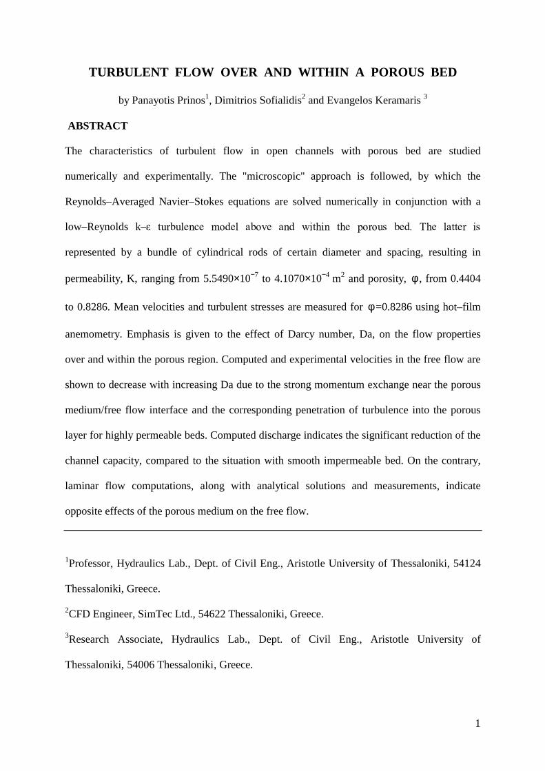
Either the "macroscopic" or "microscopic" approach can be used for the problem under

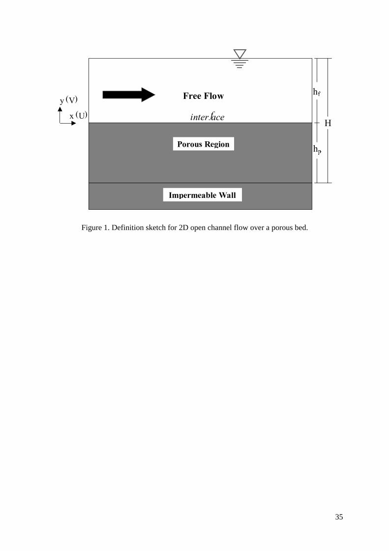
consideration (Fig. 1). The two approaches differ in the way they treat the porous layer. The

former uses macroscopic characteristics for describing the variation of flow characteristics

within the porous bed, while in the latter the flow is resolved at a local level. The governing

equations for each approach are presented in the following paragraphs together with the

advantages and drawbacks of each methodology.

Macroscopic Approach

Using this approach the turbulent flow over the porous bed is described by the RANS

equations, while the flow within the porous region is described by the extended Darcy

equation including the Forchheimer (microscopic form drag) term and the Brinkman (viscous

diffusion) term (Vafai and Tien, 1981, Vafai and Kim, 1995). The latter equation has been

extended by Antohe and Lage (1997), Nakayama and Kuwahara (1999) and Getachew et al.

(2000) for turbulent, incompressible flow in porous media. These equations, namely

continuity (eqs. (1) and (3)) and momentum (eqs. (2) and (4)), for both free flow and porous

regions (Fig. 1) are:

Free Flow Region:

0x

U

i

i =∂∂

(1)

9

−

∂∂

+∂∂

∂∂+

∂∂−=

∂∂

uux

U

x

U�

xx

P

!

1

x

UU ji

i

j

j

i

jij

ij (2)

Porous Region:

0x

U

i

i =∂∂

(3)

+φ−νφ−

−

∂∂

+∂∂

∂∂+

∂∂−=

∂∂

jijj

jijj

F2i

jii

j

j

i

jij

ij

uuUU

UUUU

K

cU

K

uux

U

x

UJ�xx

P

!

1

x

UU

(4)

where Ui=time−averaged fluid velocity in the xi direction, P=effective pressure (the difference

between the static and the hydrostatic pressure), jiuu− =Reynolds stresses, ! IOXLG�GHQVLW\��

� ���!� IOXLG� NLQHPDWLF� YLVFRVLW\�� φ =porosity, K=permeability, cF=Forchheimer (inertia)

FRHIILFLHQW�� - YLVFRVLW\� UDWLR� � �eff�����eff=effective viscosity). Ratio J can be assumed to be

equal to unity, although it was indicated that its value deviates from unity for high porosity

media (Givler and Altobelli, 1994). Eq. (4) consists of the convective inertia term in the left–

hand side and the following terms in the right–hand side: (a) pressure gradient term, (b)

Brinkman (viscous diffusion) and turbulent diffusion terms, (c) Darcy (microscopic viscous

drag) term and (d) Forchheimer (microscopic form drag) first and second order terms,

respectively. The Einstein convention is adopted for repeated indices in all equations. It

should be noted that for 2D uniform, open channel flow, the pressure gradient (–dP/dx) is

HTXDO� WR� !J6o (g=acceleration due to gravity, So=channel slope). Finally (Fig. 1),

x=streamwise and y=normal coordinates, while U and V are the corresponding velocity

components.

In order for Eqs. (1) to (4) to "close", the Reynolds stresses that appear in Eqs. (2) and (4)

have to be estimated with the aid of a turbulence model. While turbulence models for the free

10

flow region are well−established and applied in numerous cases (Rodi, 1980), macroscopic

turbulence models for flow in porous media are rather scarce. Recently, theoretical

developments of such models have been attempted by several investigators (Masuoka and

Takatsu, 1996, Antohe and Lage, 1997, Nakayama and Kawahara, 1999 and Getachew et al.,

2000) but their application is very limited.

In cases where momentum transfer from the free flow to the porous region are weak and the

penetration of turbulence into the porous region is restricted by the structure of the solid

matrix (low porosity), the flow in the porous medium is laminar and a macroscopic turbulence

model for the porous region is not required. In this case the turbulent diffusion and second

order Forchheimer terms in equation (4) are omitted and hence equation (4) can be solved in

conjunction with equations (1) (2) and (3) and appropriate matching conditions at the

porous/fluid interface (Svensson and Rahm, 1991). Also, in the case of laminar flow in both

regions the above equations are simplified into the respective Navier−Stokes equations for the

fluid region and can be solved either numerically or analytically.

Analytical solutions to the problem of laminar flow over and within a porous bed have been

derived by several investigators. Poulikakos and Kazmierczak (1987) used Eqs. (1) to (4)

(omitting the turbulent and Forchheimer terms) together with continuity interfacial conditions

for velocity and shear stress. They found analytically the velocity distribution in both fluid

and porous regions for 2D, fully developed channel flow. Such a distribution is given by the

following relationships (Fig. 1):

Fluid Region (0 ≤ y ≤ hf):

−

−

+

−−

−

−

=−

− 1

DaHh1cosh

1DaDa

Hh1tanh

HhDa

Hh

H

yh2

1

A

U

2/1f

2/1ff2/122

ff (5)

11

Porous Region (−hp ≤ y ≤ 0):

Da

DaHh1cosh

DaH

yh1sinhHhDaDa

H

ycoshDa

A

U

2/1f

2/1ff2/12/1

−

−

−−−

=−

−−

(6)

where A=(H2����G3�G[�@� DQG�'D .�+

2. In the present study, the velocity distribution in the

free flow region and the discharge capacity of the channel for laminar flow, derived by Eq.

(5), are compared with computed values calculated by the "microscopic" approach.

Microscopic Approach

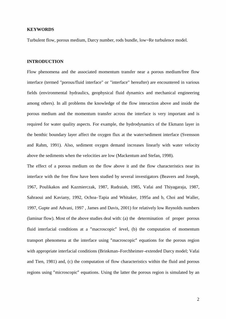
Using the "microscopic" approach the RANS eqs. (1) and (2) are solved in the whole flow

region, above the porous medium, as well as inside it. The latter, of given permeability K and

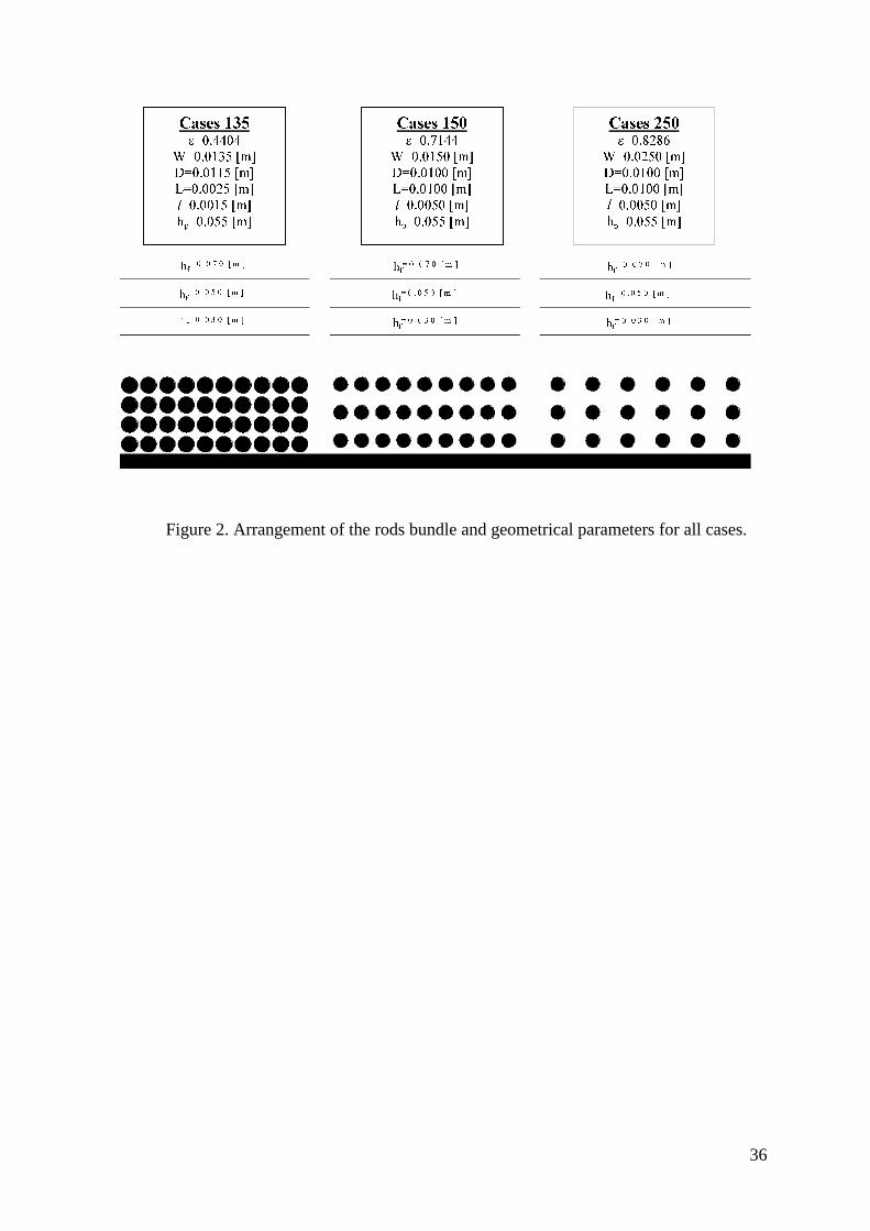
porosity φ , is simulated as a bundle of cylindrical rods (Fig. 2).

For modeling the Reynolds stresses appearing in Eq. (2), the eddy−viscosity concept is used:

k3

2

x

U

x

Uuu ij

i

j

j

itji δ−

∂∂

+∂∂ν=− (7)

ZKHUH��t HGG\�YLVFRVLW\��/ij=Kronecker delta and k=(1/2)u2i =turbulent kinetic energy.

The Launder and Sharma (1974) low Reynolds k−0�PRGHO�LV�XVHG�IRU�FDOFXODWLQJ��t. The use

of such a turbulence model is necessary in regions where turbulence is damped (near–wall

regions or low permeability porous media). The wall regions are resolved down to the solid

boundaries without using any boundary conditions for the first grid point near the wall (wall

functions). The first grid point lies well inside the viscous sublayer and hence flow

characteristics are calculated in both the viscous sub−layer and the fully turbulent flow region.

The eddy viscosity �t� LV� UHODWHG� WR� N� DQG� LWV� UDWH� RI� GLVVLSDWLRQ�� 0�� WKURXJK� WKH�

Kolmogorov−Prandtl relationship.

( )ε=ν µµ /kfc 2t (8)

12

where c�=0.09 and f�=exp[−3.4/(Rt/50)2]=damping function accounting for low−Re and

wall−proximity effectV��7KH�IROORZLQJ�WUDQVSRUW�HTXDWLRQV�IRU�N�DQG�0�DUH�VROYHG�

ε−

∂∂

σν+ν

∂∂+=

∂∂

x

k

xP

x

kU

jk

t

jk

jj (9)

kfc

xxP

kfc

xU

2

22j

t

jk11

jj

ε−

∂

ε∂

σν+ν

∂∂+ε=

∂ε∂

εεε

εε (10)

where Pk= uu ji− (∂Ui/∂xj)=production rate of k due to shear, f0�=1, f0�=1−0.3[exp(−Rt2)];

Rt=k2���0� WXUEXOHQW�5H\QROGV�QXPEHU��F0�=1.44, c0� ������1k �����DQG�10=1.3.

The interaction of the free turbulent flow with that inside the solid matrix may result in the

penetration of turbulence into the upper part of the porous medium and to increased

turbulence levels (shear stresses and intensities). Increased shear is expected to bring a

reduction of the mean velocity in the flow above the porous region and a respective increase

in the upper porous area. In other words, turbulence promotes the momentum exchange across

the interface, compared with the situation where an impermeable wall is located at the

interface. The reduction of the velocity above the porous layer implies a corresponding

reduction of the channel discharge capacity.

Opposite trends have been observed in the case of laminar flow over and within a porous bed.

Beavers and Joseph (1967) used the momentum equation for fully developed laminar flow

and an empirical porous/fluid interfacial condition and estimated an increase in mass flow

over the porous medium with regard to that with impermeable bed.

NUMERICAL PROCEDURE − BOUNDARY CONDITIONS

Eqs. (1), (2), (7), (8), (9) and (10) are solved with the CFD code FLUENT5 (1998). The grid

was dense enough near the walls, as indicated by the low s+ (=sU*/�, s=normal distance from

solid boundaries, U*=friction velocity, �=kinematic viscosity) values at the mesh nodes

13

adjacent to the walls. Provision was made in the mesh spacing in order to have at least 2÷5

nodes located inside the viscous sub–layer (s+<2).

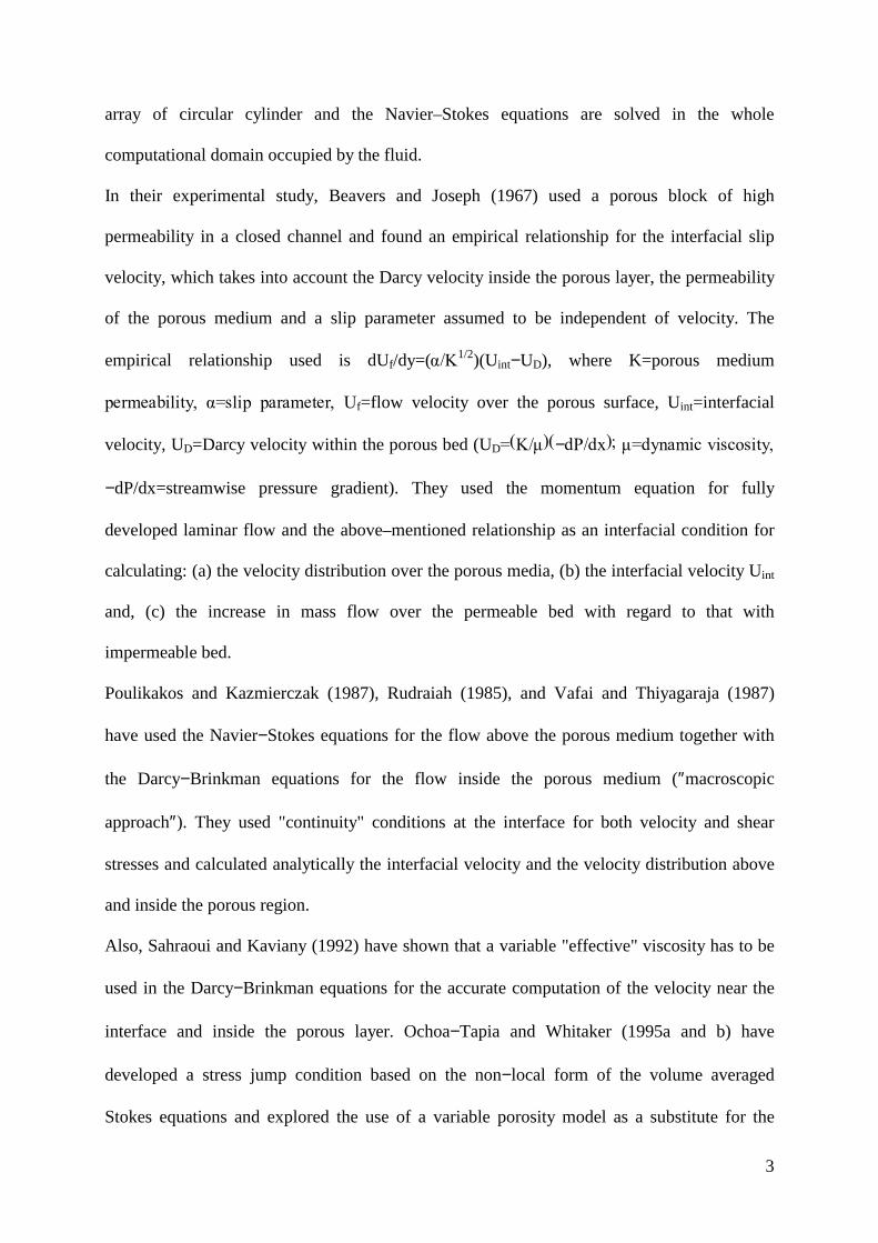
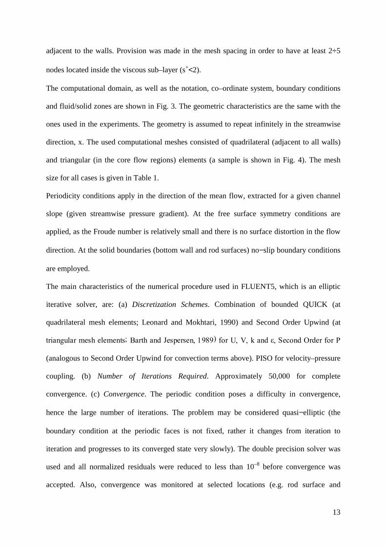
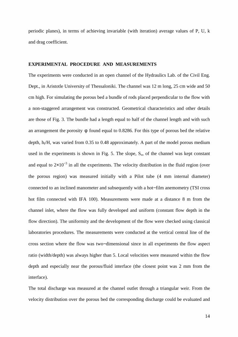
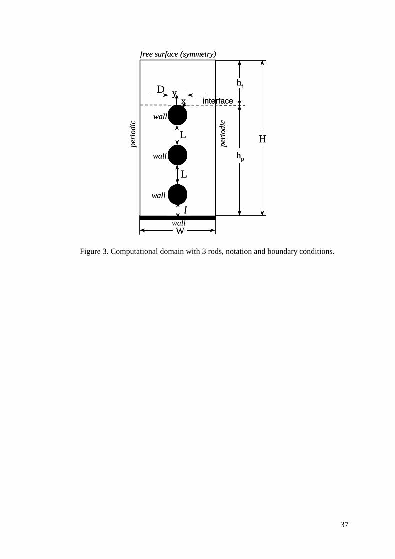
The computational domain, as well as the notation, co–ordinate system, boundary conditions

and fluid/solid zones are shown in Fig. 3. The geometric characteristics are the same with the

ones used in the experiments. The geometry is assumed to repeat infinitely in the streamwise

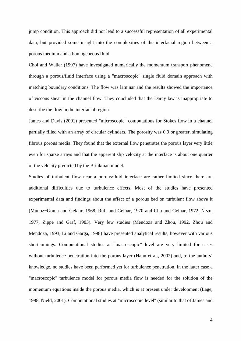
direction, x. The used computational meshes consisted of quadrilateral (adjacent to all walls)

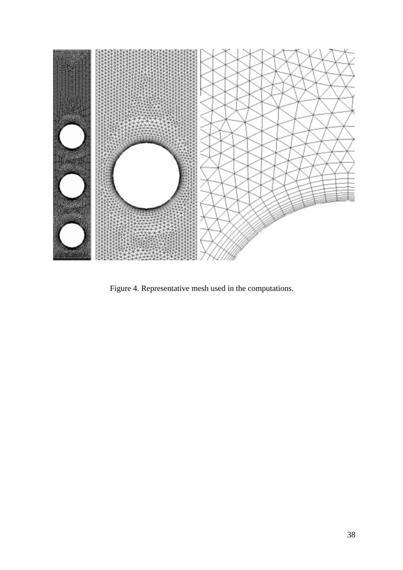
and triangular (in the core flow regions) elements (a sample is shown in Fig. 4). The mesh

size for all cases is given in Table 1.

Periodicity conditions apply in the direction of the mean flow, extracted for a given channel

slope (given streamwise pressure gradient). At the free surface symmetry conditions are

applied, as the Froude number is relatively small and there is no surface distortion in the flow

direction. At the solid boundaries (bottom wall and rod surfaces) no−slip boundary conditions

are employed.

The main characteristics of the numerical procedure used in FLUENT5, which is an elliptic

iterative solver, are: (a) Discretization Schemes. Combination of bounded QUICK (at

quadrilateral mesh elements; Leonard and Mokhtari, 1990) and Second Order Upwind (at

WULDQJXODU�PHVK�HOHPHQWV��%DUWK�DQG�-HVSHUVHQ��������IRU�8��9��N�DQG�0��6HFRQG�2UGHU�IRU�3�

(analogous to Second Order Upwind for convection terms above). PISO for velocity–pressure

coupling. (b) Number of Iterations Required. Approximately 50,000 for complete

convergence. (c) Convergence. The periodic condition poses a difficulty in convergence,

hence the large number of iterations. The problem may be considered quasi−elliptic (the

boundary condition at the periodic faces is not fixed, rather it changes from iteration to

iteration and progresses to its converged state very slowly). The double precision solver was

used and all normalized residuals were reduced to less than 10–8 before convergence was

accepted. Also, convergence was monitored at selected locations (e.g. rod surface and

14

periodic planes), in terms of achieving invariable (with iteration) average values of P, U, k

and drag coefficient.

EXPERIMENTAL PROCEDURE AND MEASUREMENTS

The experiments were conducted in an open channel of the Hydraulics Lab. of the Civil Eng.

Dept., in Aristotle University of Thessaloniki. The channel was 12 m long, 25 cm wide and 50

cm high. For simulating the porous bed a bundle of rods placed perpendicular to the flow with

a non-staggered arrangement was constructed. Geometrical characteristics and other details

are those of Fig. 3. The bundle had a length equal to half of the channel length and with such

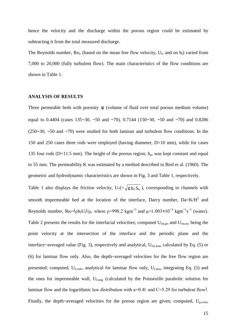
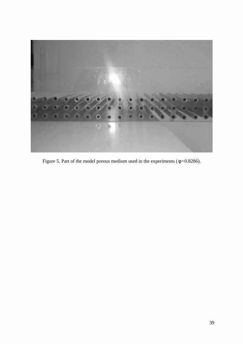
an arrangement the porosity φ found equal to 0.8286. For this type of porous bed the relative

depth, hf/H, was varied from 0.35 to 0.48 approximately. A part of the model porous medium

used in the experiments is shown in Fig. 5. The slope, So, of the channel was kept constant

and equal to 2×10−3 in all the experiments. The velocity distribution in the fluid region (over

the porous region) was measured initially with a Pilot tube (4 mm internal diameter)

connected to an inclined manometer and subsequently with a hot−film anemometry (TSI cross

hot film connected with IFA 100). Measurements were made at a distance 8 m from the

channel inlet, where the flow was fully developed and uniform (constant flow depth in the

flow direction). The uniformity and the development of the flow were checked using classical

laboratories procedures. The measurements were conducted at the vertical central line of the

cross section where the flow was two−dimensional since in all experiments the flow aspect

ratio (width/depth) was always higher than 5. Local velocities were measured within the flow

depth and especially near the porous/fluid interface (the closest point was 2 mm from the

interface).

The total discharge was measured at the channel outlet through a triangular weir. From the

velocity distribution over the porous bed the corresponding discharge could be evaluated and

15

hence the velocity and the discharge within the porous region could be estimated by

subtracting it from the total measured discharge.

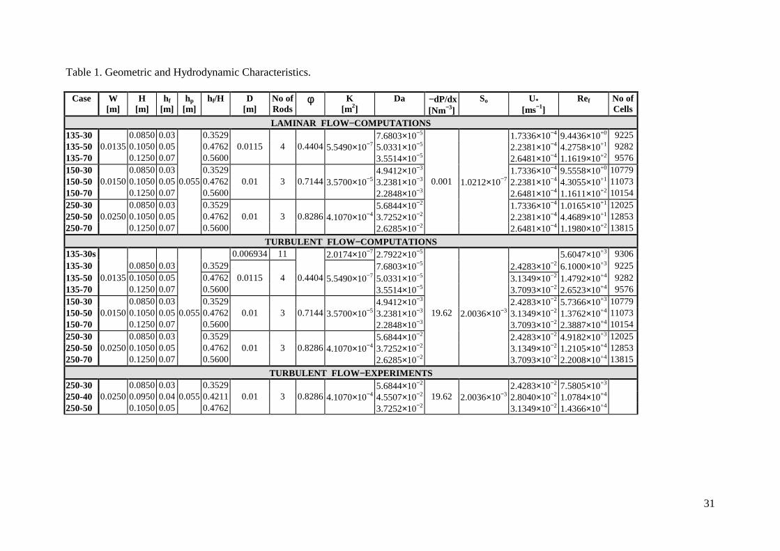
The Reynolds number, Ref, (based on the mean free flow velocity, Uf, and on hf) varied from

7,000 to 20,000 (fully turbulent flow). The main characteristics of the flow conditions are

shown in Table 1.

ANALYSIS OF RESULTS

Three permeable beds with porosity φ (volume of fluid over total porous medium volume)

equal to 0.4404 (cases 135−30, −50 and −70), 0.7144 (150−30, −50 and −70) and 0.8286

(250−30, −50 and −70) were studied for both laminar and turbulent flow conditions. In the

150 and 250 cases three rods were employed (having diameter, D=10 mm), while for cases

135 four rods (D=11.5 mm). The height of the porous region, hp, was kept constant and equal

to 55 mm. The permeability K was estimated by a method described in Bird et al. (1960). The

geometric and hydrodynamic characteristics are shown in Fig. 3 and Table 1, respectively.

Table 1 also displays the friction velocity, U*(= Shg of ), corresponding to channels with

smooth impermeable bed at the location of the interface, Darcy number, Da=K/H2 and

Reynolds number, Ref �!KfUf�����ZKHUH�! ������NJP−3�DQG�� �����×10−3 kgm−1s−1 (water).

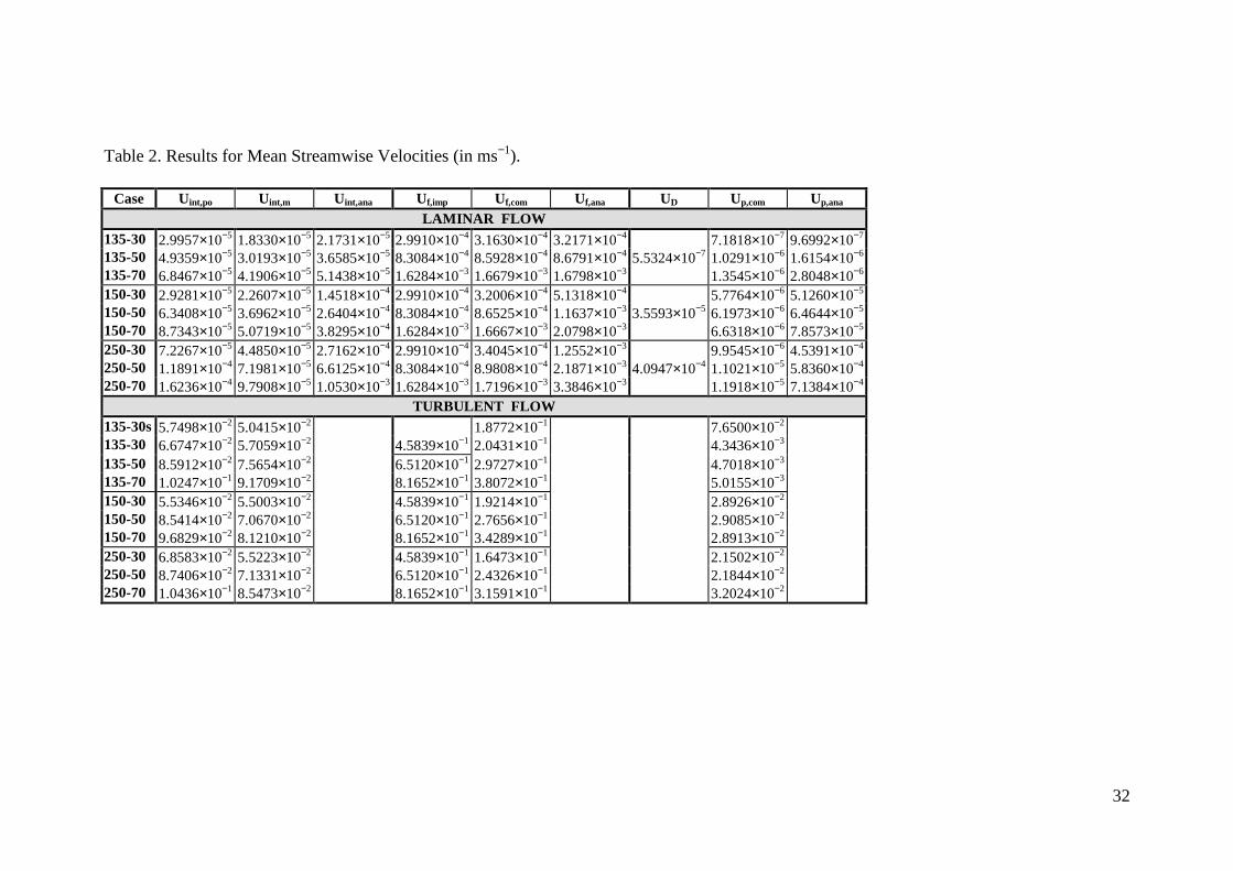
Table 2 presents the results for the interfacial velocities; computed Uint,po and Uint,m, being the

point velocity at the intersection of the interface and the periodic plane and the

interface−averaged value (Fig. 3), respectively and analytical, Uint,ana, calculated by Eq. (5) or

(6) for laminar flow only. Also, the depth−averaged velocities for the free flow region are

presented; computed, Uf,com, analytical for laminar flow only, Uf,ana, integrating Eq. (5) and

the ones for impermeable wall, Uf,imp (calculated by the Poisseuille parabolic solution for

laminar flow and the logarithmic�ODZ�GLVWULEXWLRQ�ZLWK�� �����DQG�& �����IRU�WXUEXOHQW�IORZ���

Finally, the depth−averaged velocities for the porous region are given; computed, Up,com,

16

analytical for laminar flow only, Up,ana, integrating Eq. (6) and the Darcy one for laminar flow

only, UD �.����−dP/dx).

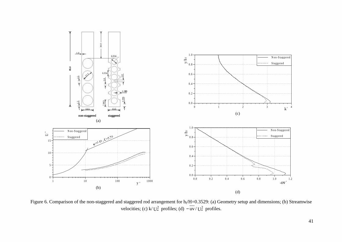
The effect of cylinders arrangement (structure of the model porous medium) on the flow

characteristics was studied initially by using a staggered (case 135–30s)and non–staggered

(case 135–30) arrangement (Figure 6a) with different rods diameter but the same porosity

(φ =0.4404). Figure 6b shows the velocity distribution above the porous region in wall

coordinates for both arrangements. In both cases velocities are much lower than the respective

ones for flow over a smooth impermeable bed with flow depth hf. There is a small difference

in velocities between the two arrangements which is attributed to the slightly different Darcy

numbers (different permeabilities) due to the different rods diameter. Similar conclusions can

be derived from the comparison of the computed turbulence kinetic energy and shear stress

for both arrangements (Figures 6c and 6d).

In the following figures computed results using the non-staggered arrangement are presented.

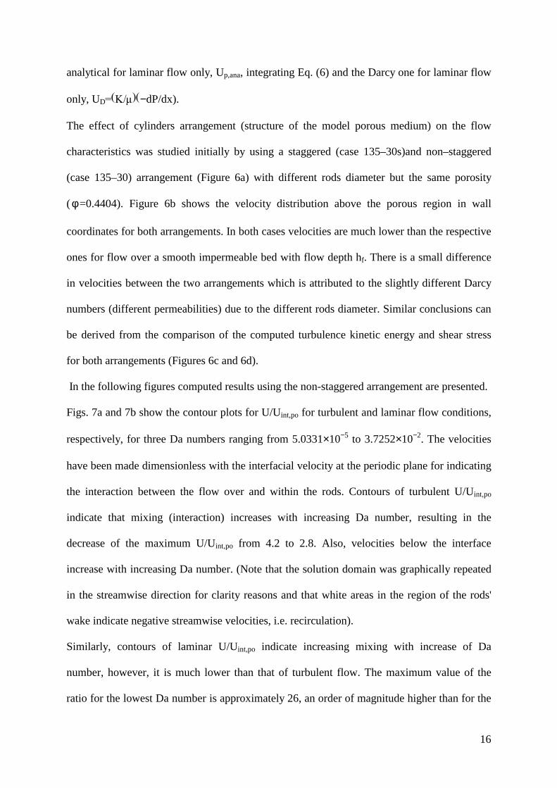
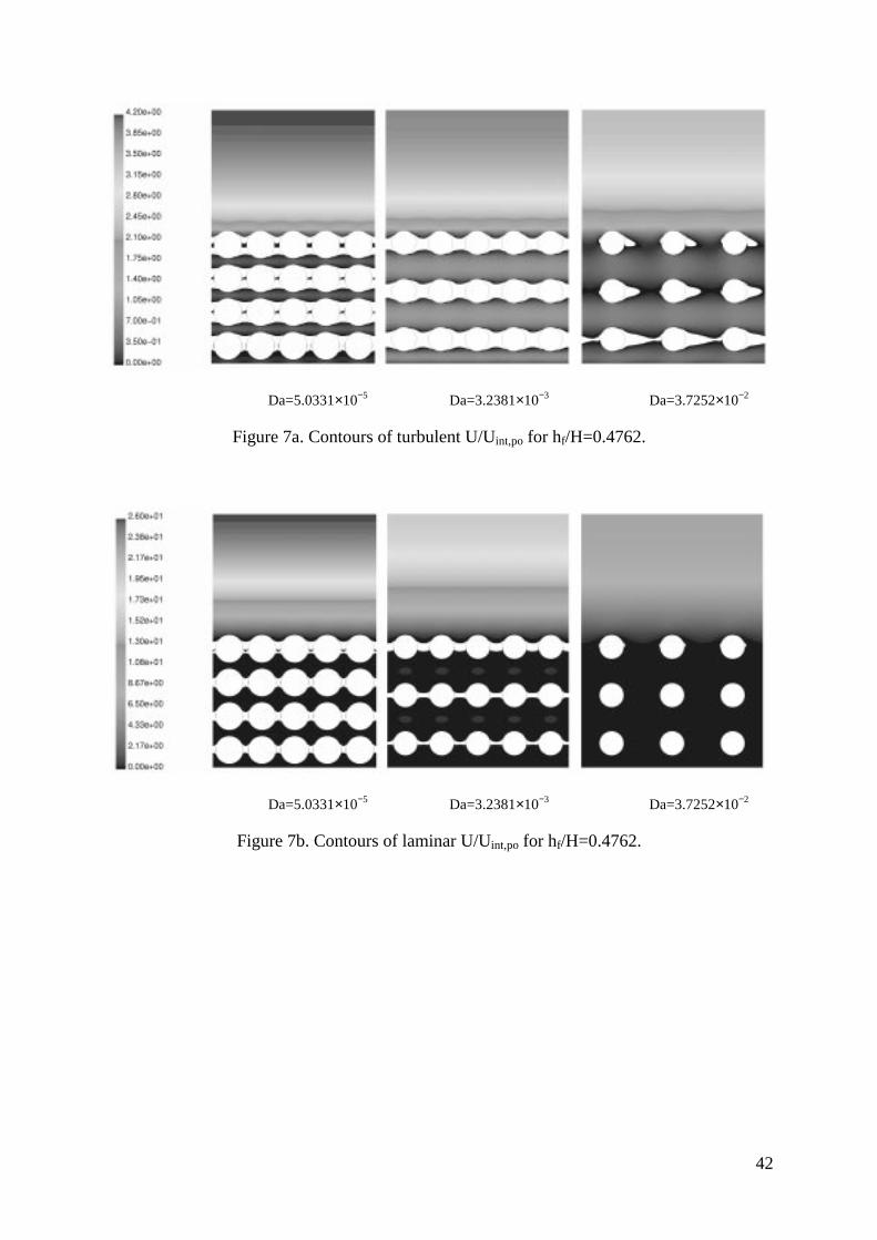
Figs. 7a and 7b show the contour plots for U/Uint,po for turbulent and laminar flow conditions,

respectively, for three Da numbers ranging from 5.0331×10−5 to 3.7252×10−2. The velocities

have been made dimensionless with the interfacial velocity at the periodic plane for indicating

the interaction between the flow over and within the rods. Contours of turbulent U/Uint,po

indicate that mixing (interaction) increases with increasing Da number, resulting in the

decrease of the maximum U/Uint,po from 4.2 to 2.8. Also, velocities below the interface

increase with increasing Da number. (Note that the solution domain was graphically repeated

in the streamwise direction for clarity reasons and that white areas in the region of the rods'

wake indicate negative streamwise velocities, i.e. recirculation).

Similarly, contours of laminar U/Uint,po indicate increasing mixing with increase of Da

number, however, it is much lower than that of turbulent flow. The maximum value of the

ratio for the lowest Da number is approximately 26, an order of magnitude higher than for the

17

corresponding turbulent case. With increasing Da number this value drops to approximately

13, being again much higher than the respective value for turbulent flow.

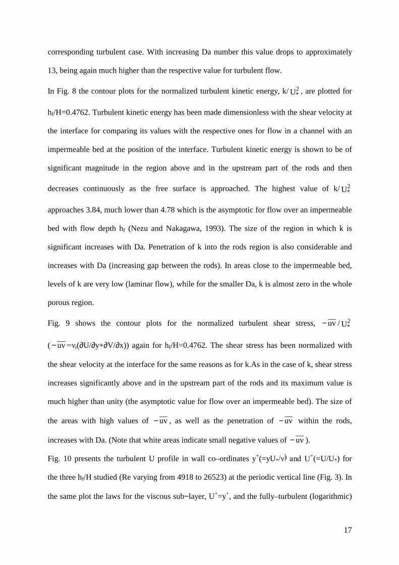
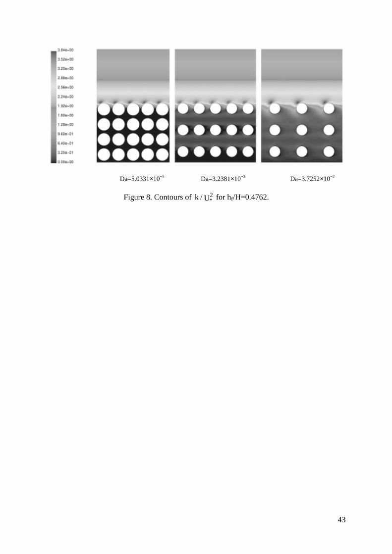
In Fig. 8 the contour plots for the normalized turbulent kinetic energy, k/U2* , are plotted for

hf/H=0.4762. Turbulent kinetic energy has been made dimensionless with the shear velocity at

the interface for comparing its values with the respective ones for flow in a channel with an

impermeable bed at the position of the interface. Turbulent kinetic energy is shown to be of

significant magnitude in the region above and in the upstream part of the rods and then

decreases continuously as the free surface is approached. The highest value of k/U2*

approaches 3.84, much lower than 4.78 which is the asymptotic for flow over an impermeable

bed with flow depth hf (Nezu and Nakagawa, 1993). The size of the region in which k is

significant increases with Da. Penetration of k into the rods region is also considerable and

increases with Da (increasing gap between the rods). In areas close to the impermeable bed,

levels of k are very low (laminar flow), while for the smaller Da, k is almost zero in the whole

porous region.

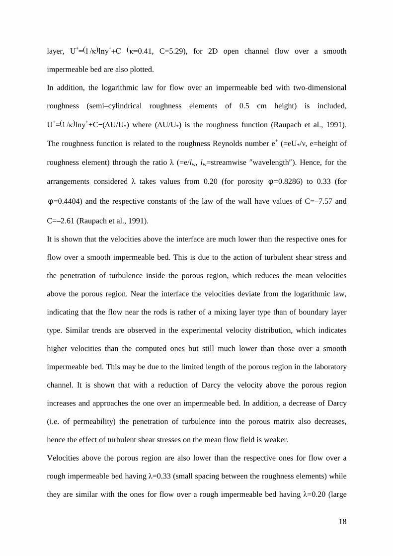
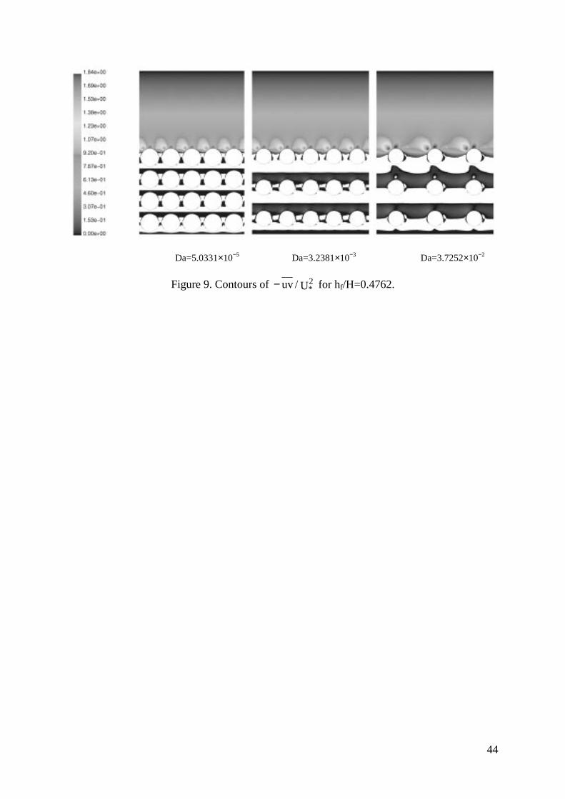
Fig. 9 shows the contour plots for the normalized turbulent shear stress, uv− / U2*

( uv− �t(∂U/∂y+∂V/∂x)) again for hf/H=0.4762. The shear stress has been normalized with

the shear velocity at the interface for the same reasons as for k.As in the case of k, shear stress

increases significantly above and in the upstream part of the rods and its maximum value is

much higher than unity (the asymptotic value for flow over an impermeable bed). The size of

the areas with high values of uv− , as well as the penetration of uv− within the rods,

increases with Da. (Note that white areas indicate small negative values of uv− ).

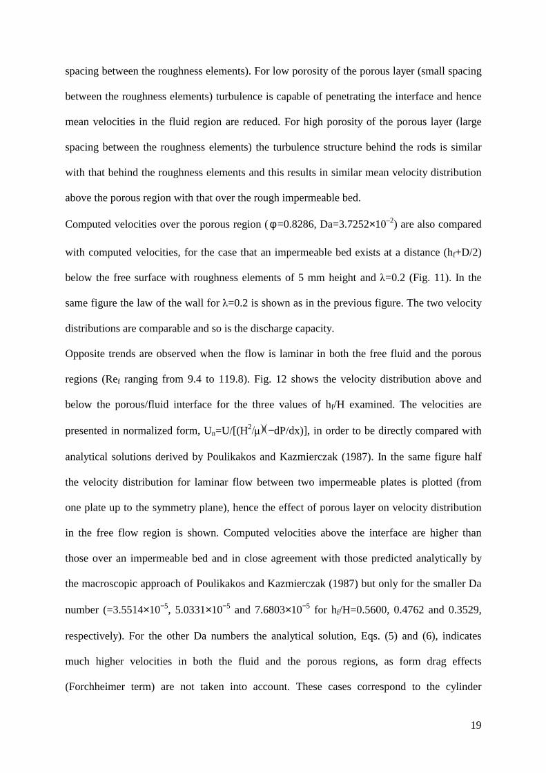
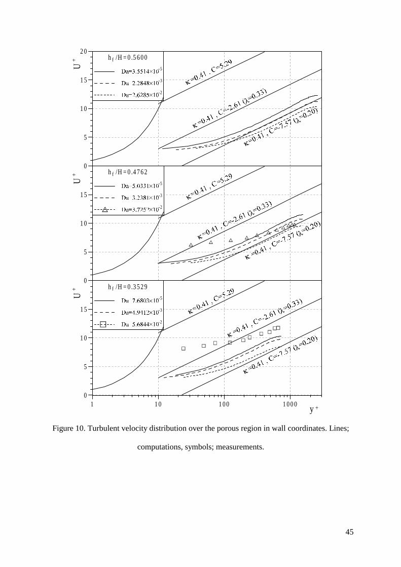
Fig. 10 presents the turbulent U profile in wall co–ordinates y+(=yU*���� DQG�8+(=U/U*) for

the three hf/H studied (Re varying from 4918 to 26523) at the periodic vertical line (Fig. 3). In

the same plot the laws for the viscous sub−layer, U+=y+, and the fully–turbulent (logarithmic)

18

layer, U+ �����OQ\

+�&� �� 0.41, C=5.29), for 2D open channel flow over a smooth

impermeable bed are also plotted.

In addition, the logarithmic law for flow over an impermeable bed with two-dimensional

roughness (semi–cylindrical roughness elements of 0.5 cm height) is included,

U+=�����OQ\++C−(ûU/U*) where (ûU/U*) is the roughness function (Raupach et al., 1991).

The roughness function is related to the roughness Reynolds number e+ (=eU*/�, e=height of

roughness element) through the ratio � (=e/lw, lw=streamwise ″wavelength″). Hence, for the

arrangements considered � takes values from 0.20 (for porosity φ =0.8286) to 0.33 (for

φ =0.4404) and the respective constants of the law of the wall have values of C=–7.57 and

C=–2.61 (Raupach et al., 1991).

It is shown that the velocities above the interface are much lower than the respective ones for

flow over a smooth impermeable bed. This is due to the action of turbulent shear stress and

the penetration of turbulence inside the porous region, which reduces the mean velocities

above the porous region. Near the interface the velocities deviate from the logarithmic law,

indicating that the flow near the rods is rather of a mixing layer type than of boundary layer

type. Similar trends are observed in the experimental velocity distribution, which indicates

higher velocities than the computed ones but still much lower than those over a smooth

impermeable bed. This may be due to the limited length of the porous region in the laboratory

channel. It is shown that with a reduction of Darcy the velocity above the porous region

increases and approaches the one over an impermeable bed. In addition, a decrease of Darcy

(i.e. of permeability) the penetration of turbulence into the porous matrix also decreases,

hence the effect of turbulent shear stresses on the mean flow field is weaker.

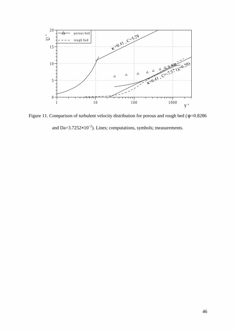
Velocities above the porous region are also lower than the respective ones for flow over a

rough impermeable bed having �=0.33 (small spacing between the roughness elements) while

they are similar with the ones for flow over a rough impermeable bed having �=0.20 (large

19

spacing between the roughness elements). For low porosity of the porous layer (small spacing

between the roughness elements) turbulence is capable of penetrating the interface and hence

mean velocities in the fluid region are reduced. For high porosity of the porous layer (large

spacing between the roughness elements) the turbulence structure behind the rods is similar

with that behind the roughness elements and this results in similar mean velocity distribution

above the porous region with that over the rough impermeable bed.

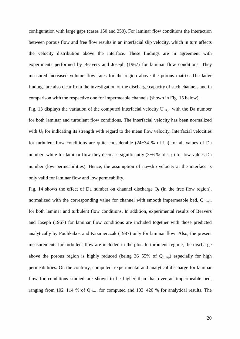
Computed velocities over the porous region (φ =0.8286, Da=3.7252×10–2) are also compared

with computed velocities, for the case that an impermeable bed exists at a distance (hf+D/2)

below the free surface with roughness elements of 5 mm height and �=0.2 (Fig. 11). In the

same figure the law of the wall for �=0.2 is shown as in the previous figure. The two velocity

distributions are comparable and so is the discharge capacity.

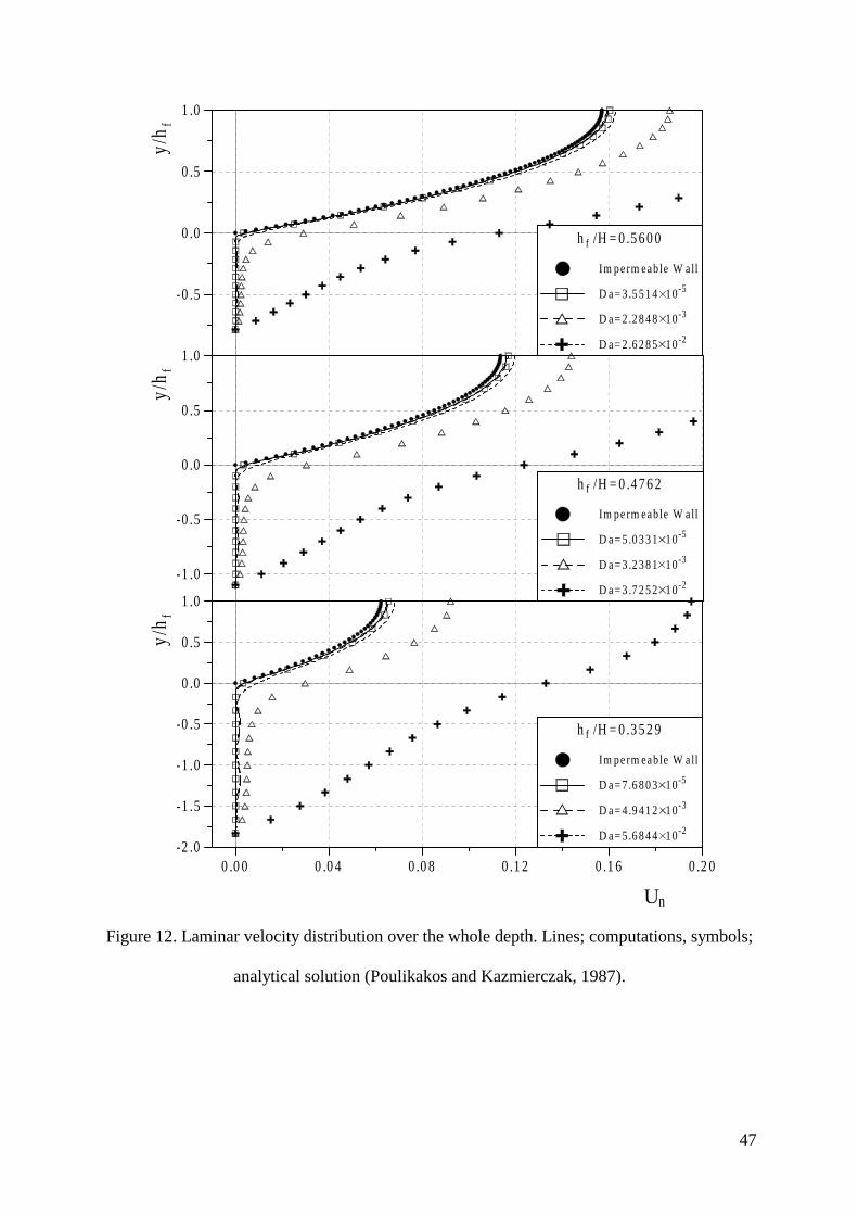
Opposite trends are observed when the flow is laminar in both the free fluid and the porous

regions (Ref ranging from 9.4 to 119.8). Fig. 12 shows the velocity distribution above and

below the porous/fluid interface for the three values of hf/H examined. The velocities are

presented in normalized form, Un=U/[(H2����−dP/dx)], in order to be directly compared with

analytical solutions derived by Poulikakos and Kazmierczak (1987). In the same figure half

the velocity distribution for laminar flow between two impermeable plates is plotted (from

one plate up to the symmetry plane), hence the effect of porous layer on velocity distribution

in the free flow region is shown. Computed velocities above the interface are higher than

those over an impermeable bed and in close agreement with those predicted analytically by

the macroscopic approach of Poulikakos and Kazmierczak (1987) but only for the smaller Da

number (=3.5514×10−5, 5.0331×10−5 and 7.6803×10−5 for hf/H=0.5600, 0.4762 and 0.3529,

respectively). For the other Da numbers the analytical solution, Eqs. (5) and (6), indicates

much higher velocities in both the fluid and the porous regions, as form drag effects

(Forchheimer term) are not taken into account. These cases correspond to the cylinder

20

configuration with large gaps (cases 150 and 250). For laminar flow conditions the interaction

between porous flow and free flow results in an interfacial slip velocity, which in turn affects

the velocity distribution above the interface. These findings are in agreement with

experiments performed by Beavers and Joseph (1967) for laminar flow conditions. They

measured increased volume flow rates for the region above the porous matrix. The latter

findings are also clear from the investigation of the discharge capacity of such channels and in

comparison with the respective one for impermeable channels (shown in Fig. 15 below).

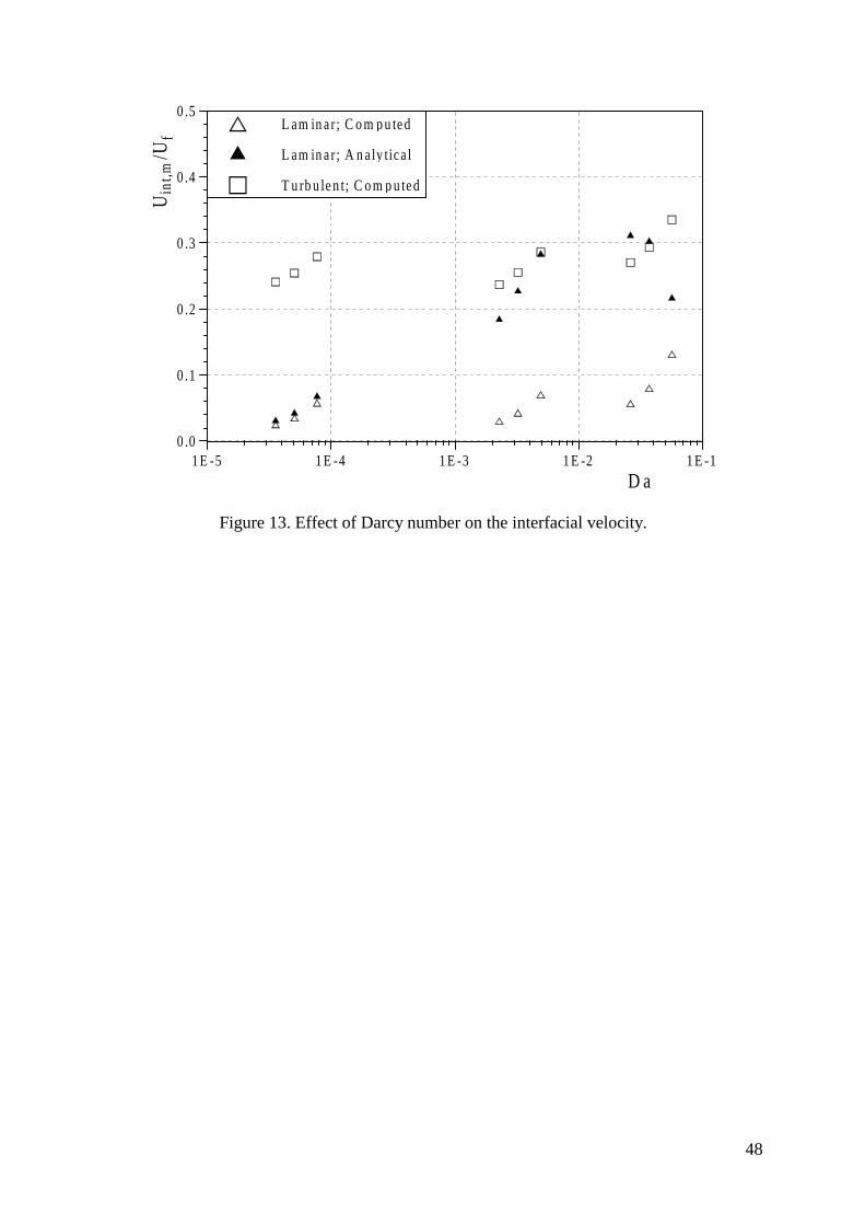
Fig. 13 displays the variation of the computed interfacial velocity Uint,m with the Da number

for both laminar and turbulent flow conditions. The interfacial velocity has been normalized

with Uf for indicating its strength with regard to the mean flow velocity. Interfacial velocities

for turbulent flow conditions are quite considerable (24−34 % of Uf) for all values of Da

number, while for laminar flow they decrease significantly (3−6 % of Uf ) for low values Da

number (low permeabilities). Hence, the assumption of no−slip velocity at the interface is

only valid for laminar flow and low permeability.

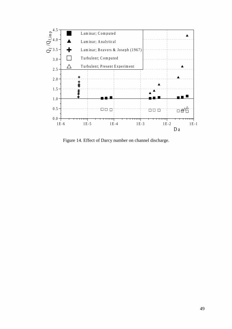
Fig. 14 shows the effect of Da number on channel discharge Qf (in the free flow region),

normalized with the corresponding value for channel with smooth impermeable bed, Qf,imp,

for both laminar and turbulent flow conditions. In addition, experimental results of Beavers

and Joseph (1967) for laminar flow conditions are included together with those predicted

analytically by Poulikakos and Kazmierczak (1987) only for laminar flow. Also, the present

measurements for turbulent flow are included in the plot. In turbulent regime, the discharge

above the porous region is highly reduced (being 36−55% of Qf,imp) especially for high

permeabilities. On the contrary, computed, experimental and analytical discharge for laminar

flow for conditions studied are shown to be higher than that over an impermeable bed,

ranging from 102−114 % of Qf,imp for computed and 103−420 % for analytical results. The

21

higher rates predicted analytically by Poulikakos and Kazmierczak (1987) for some cases are

due to the assumptions involved in their analytical derivation (no form drag effects included).

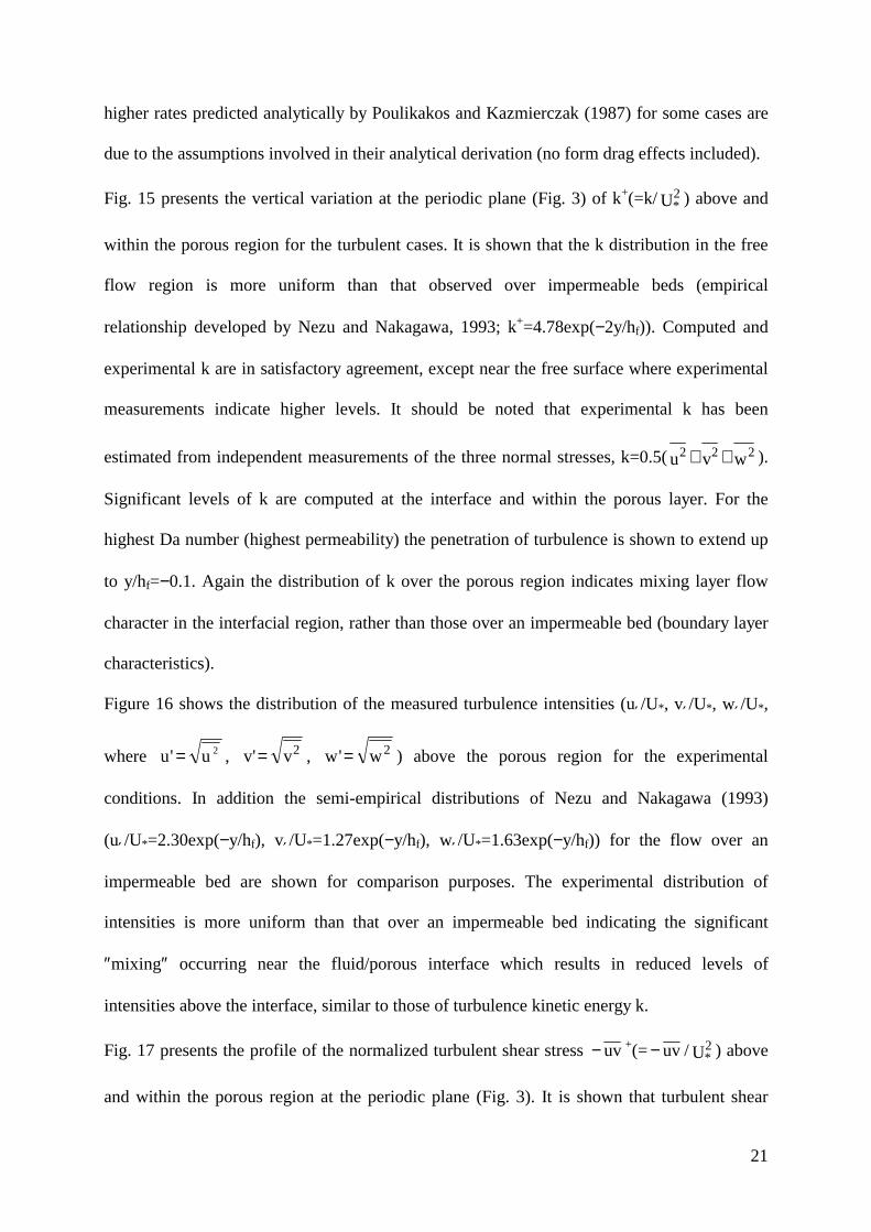
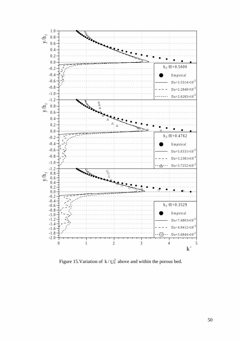
Fig. 15 presents the vertical variation at the periodic plane (Fig. 3) of k+(=k/ U2* ) above and

within the porous region for the turbulent cases. It is shown that the k distribution in the free

flow region is more uniform than that observed over impermeable beds (empirical

relationship developed by Nezu and Nakagawa, 1993; k+=4.78exp(−2y/hf)). Computed and

experimental k are in satisfactory agreement, except near the free surface where experimental

measurements indicate higher levels. It should be noted that experimental k has been

estimated from independent measurements of the three normal stresses, k=0.5(wvu 222 ++ ).

Significant levels of k are computed at the interface and within the porous layer. For the

highest Da number (highest permeability) the penetration of turbulence is shown to extend up

to y/hf=−0.1. Again the distribution of k over the porous region indicates mixing layer flow

character in the interfacial region, rather than those over an impermeable bed (boundary layer

characteristics).

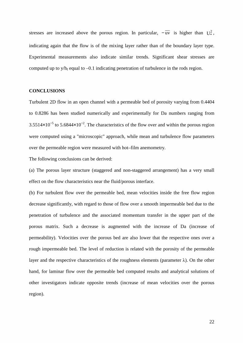
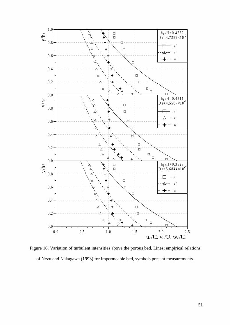
Figure 16 shows the distribution of the measured turbulence intensities (uï/U*, vï/U*, wï/U*,

where 2u'u = , 2v'v = , 2w'w = ) above the porous region for the experimental

conditions. In addition the semi-empirical distributions of Nezu and Nakagawa (1993)

(uï/U*=2.30exp(−y/hf), vï/U*=1.27exp(−y/hf), wï/U*=1.63exp(−y/hf)) for the flow over an

impermeable bed are shown for comparison purposes. The experimental distribution of

intensities is more uniform than that over an impermeable bed indicating the significant

″mixing″ occurring near the fluid/porous interface which results in reduced levels of

intensities above the interface, similar to those of turbulence kinetic energy k.

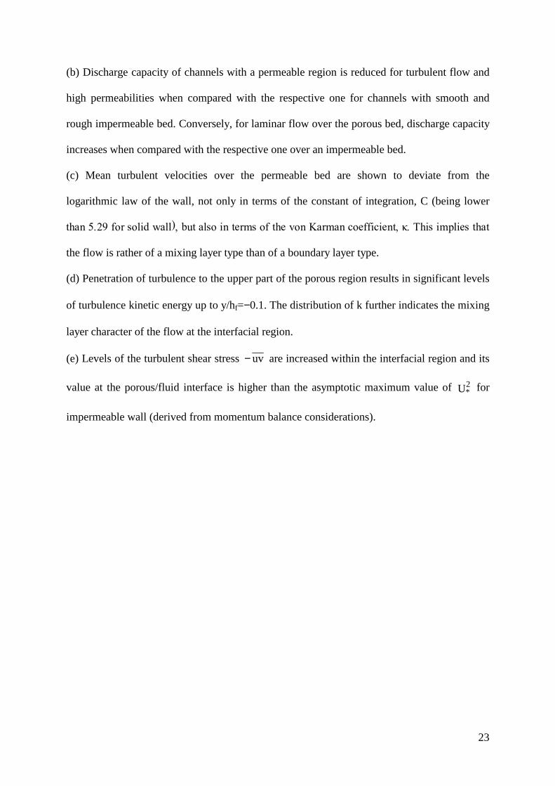
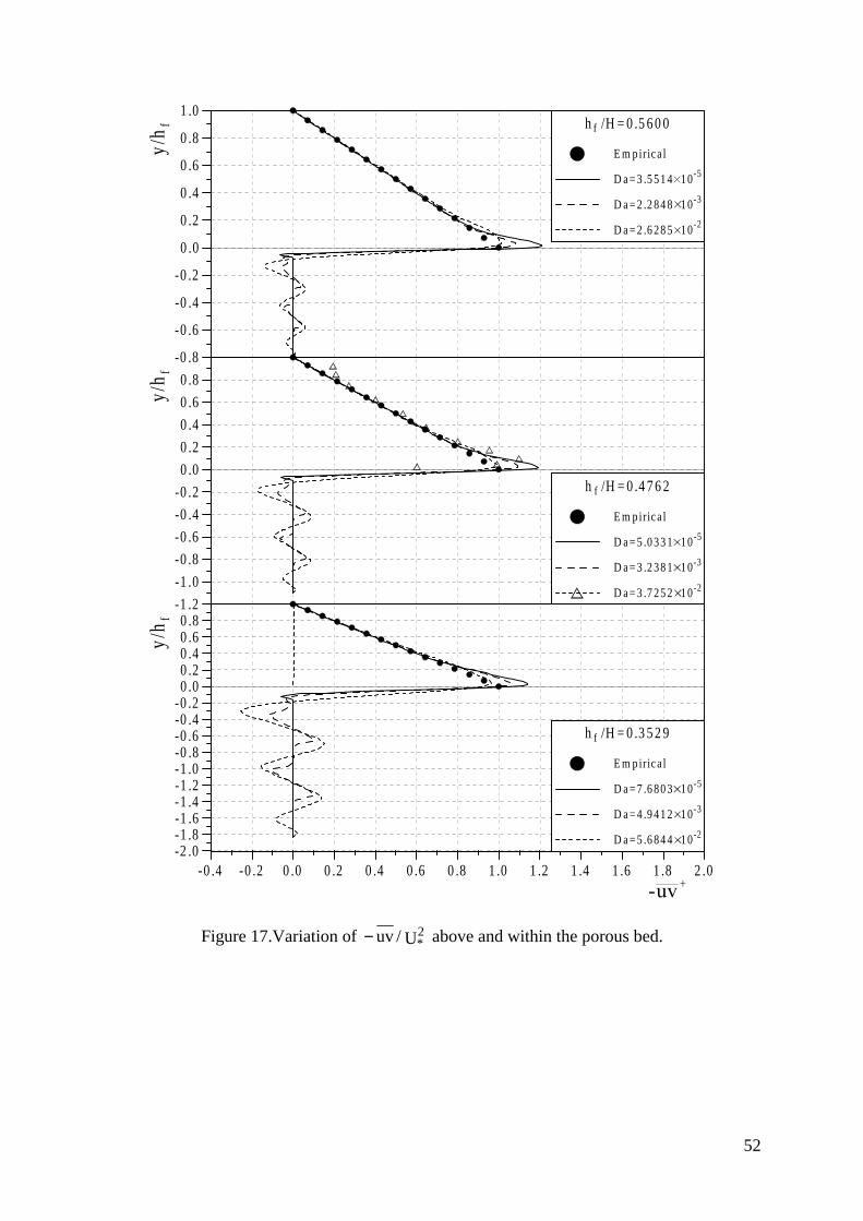
Fig. 17 presents the profile of the normalized turbulent shear stress uv− +(= uv− / U2* ) above

and within the porous region at the periodic plane (Fig. 3). It is shown that turbulent shear

22

stresses are increased above the porous region. In particular, uv− is higher than U2* ,

indicating again that the flow is of the mixing layer rather than of the boundary layer type.

Experimental measurements also indicate similar trends. Significant shear stresses are

computed up to y/hf equal to –0.1 indicating penetration of turbulence in the rods region.

CONCLUSIONS

Turbulent 2D flow in an open channel with a permeable bed of porosity varying from 0.4404

to 0.8286 has been studied numerically and experimentally for Da numbers ranging from

3.5514×10−5 to 5.6844×10−2. The characteristics of the flow over and within the porous region

were computed using a "microscopic" approach, while mean and turbulence flow parameters

over the permeable region were measured with hot–film anemometry.

The following conclusions can be derived:

(a) The porous layer structure (staggered and non-staggered arrangement) has a very small

effect on the flow characteristics near the fluid/porous interface.

(b) For turbulent flow over the permeable bed, mean velocities inside the free flow region

decrease significantly, with regard to those of flow over a smooth impermeable bed due to the

penetration of turbulence and the associated momentum transfer in the upper part of the

porous matrix. Such a decrease is augmented with the increase of Da (increase of

permeability). Velocities over the porous bed are also lower that the respective ones over a

rough impermeable bed. The level of reduction is related with the porosity of the permeable

layer and the respective characteristics of the roughness elements (parameter �). On the other

hand, for laminar flow over the permeable bed computed results and analytical solutions of

other investigators indicate opposite trends (increase of mean velocities over the porous

region).

23

(b) Discharge capacity of channels with a permeable region is reduced for turbulent flow and

high permeabilities when compared with the respective one for channels with smooth and

rough impermeable bed. Conversely, for laminar flow over the porous bed, discharge capacity

increases when compared with the respective one over an impermeable bed.

(c) Mean turbulent velocities over the permeable bed are shown to deviate from the

logarithmic law of the wall, not only in terms of the constant of integration, C (being lower

WKDQ������IRU�VROLG�ZDOO���EXW�DOVR�LQ�WHUPV�RI�WKH�YRQ�.DUPDQ�FRHIILFLHQW�����7KLV�LPSOLHV�WKDW�

the flow is rather of a mixing layer type than of a boundary layer type.

(d) Penetration of turbulence to the upper part of the porous region results in significant levels

of turbulence kinetic energy up to y/hf=−0.1. The distribution of k further indicates the mixing

layer character of the flow at the interfacial region.

(e) Levels of the turbulent shear stress uv− are increased within the interfacial region and its

value at the porous/fluid interface is higher than the asymptotic maximum value of U2* for

impermeable wall (derived from momentum balance considerations).

24

APPENDIX I: REFERENCES

Antohe, B. V., and Lage, J. L. (1997). "A general two−equation macroscopic turbulence

model for incompressible flow in porous media." Int. J. Heat and Mass Transfer, 40(13),

3013−3024.

Barth, T. J., and Jespersen, D. (1989). "The design and application of upwind schemes on

unstructured meshes." Technical Report AIAA–89–0366, AIAA 27th Aerospace Sciences

Meeting, Reno, Nevada.

Beavers, G. S., and Joseph, D. D. (1967). "Boundary conditions at a naturally permeable

wall." J. Fluid Mech., 30(1), 197–207.

Bird, R. B., Stewart, W. E., and Lighfoot, E. N. (1960). Transport phenomena. Wiley, New

York.

Choi, C. Y., and Waller, P. M. (1997). "Momentum transport mechanism for water flow over

porous media." J. Environmental Engrg., ASCE, 123(8), 792–799.

Chu, Y. H., and Gelhar, L. W. (1972). "Turbulent Pipe Flow with Granular Permeable

Boundaries." Rep. No. 148, Ralph M. Parsons Lab. for Water Resources and Hydrodynamics,

Dept. of Civil Engrg., M.I.T., Cambridge, Massachusetts.

FLUENT 5 User's Guide (1998). Fluent Inc., Lebanon, N.H.

Getachew, D., Minkowycz, W. J., and Lage, J. L. (2000). "A modified form of the k−0�PRGHO�

for turbulent flows of an incompressible fluid in porous media." Int. J. Heat and Mass

Transfer, 43(16), 2909−2915.

Givler, R. C., and Altobelli, S. A. (1994). "A determination of the effective viscosity for the

Brinkman−Forchheimer flow model." J. Fluid Mech., 258, 355−370.

Gupte, S. K., and Advani, S. G. (1997). "Flow near the permeable boundary of a porous

medium: An experimental investigation using LDA." Experiments in Fluids, 22, 408–414.

25

Hahn, S., Je, J., and Choi, H. (2002). "Direct numerical simulation of turbulent channel flow

with permeable walls." J. Fluid Mech., 450, 259–285.

James, D. F., and Davis, A. M. (2001). "Flow at the interface of a model fibrous porous

medium." J. Fluid Mech., 426, 47–72.

Keramaris, E. (2001). "Turbulent flow in an open channel with a porous bed." Ph.D Thesis,

Dept. of Civil Eng., Aristotle University of Thessaloniki (in Greek).

Lage, J. L. (1998). "The fundamental theory of flow through permeable media: from Darcy to

turbulence." Transport Phenomena in Porous Media, D.B. Ingham and I. Pop, eds., Elsevier

Science, Oxford, 1–30.

Launder, B. E., and Sharma, B. I. (1974), "Application of the energy−dissipation model of

turbulence to the calculation of flow near a spinning disk." Letters in Heat and Mass Transfer,

3, 269−289.

Leonard, B. P., and Mokhtari, S. (1990). "ULTRA–SHARP Nonoscillatory convection

schemes for high–speed steady multidimensional flow." NASA TM 1–2568 (ICOMP–90–12),

NASA Lewis Research Center.

Li, B. (1990). "Characteristics of flow in rough channels with permeable bed." Proc., 7th

Congress APD−IAHR, Chinese Association for Hydraulic Research, Beijing, China, 1–7.

Li, B., and Garga, V. K. (1998). "Theoretical solution for seepage flow in overtopped

rockfill." J. Hydraulic Engrg., ASCE, 124(2), 213–217.

Mackentun, A. A., and Stefan, H. G. (1998). "Effect of flow velocity on sediment oxygen

demand: Experiments." J. Environmental Engrg., ASCE, 124(3), 222–230.

Masuoka, T., and Takatsu, Y. (1996). "Turbulence model for flow through porous media." Int.

J. Heat and Mass Transfer, 39(13), 2803−2809.

Mendoza, C., and Zhou, D. (1992). "Effects of porous bed on turbulent stream flow above

bed." J. Hydraulic Engrg., ASCE, 118(9), 1222–1240.

26

Munoz−Goma, R. J., and Gelhar, L. W. (1968). "Turbulent pipe flow with rough and porous

walls." Rep. No. 109, Hydrodynamics Lab., Dept. of Civil Engrg., M.I.T., Cambridge,

Massachusetts.

Nakamura, Y., and Stefan, H. G. (1994). "Effect of flow velocity on sediment oxygen

demand: Theory." J. Environmental Engrg., ASCE, 120(5), 996−1016.

Nakamura, Y., Yanagimachi, T., and Inone, T. (1996). "Effect of surface roughness on mass

transfer at the sediment water interface." Proc., Int. Conf. on Flow Modelling and Turbulent

Measurements, Tallahassee, Florida, 805−812.

Nakayama, A., and Kuwahara, F. (1999). "A macroscopic turbulence model for flow in a

porous medium." J. Fluids Engrg., ASME, 121(2), 427−433.

Nezu, I. (1977). "Turbulent Structure in Open–Channel Flows." PhD thesis, Dept. of

Civil.Engineering, Kyoto Univ., Japan.

Nezu, I., and Nakagawa, H. (1993). Turbulence in open channel flow. IAHR monograph,

Balkema Pub. , Rotterdam. The Netherlands.

Nield, D. A. (2001). "Alternative models of turbulence in a porous medium and related

matters." J. of Fluids Engrg., Transactions of the ASME, 123, 928–934.

Ochoa−Tapia, A. J., and Whitaker, S. (1995a). "Momentum transfer at the boundary between

a porous medium and a homogeneous fluid. I: Theoretical development." Int. J. Heat Mass

Transfer, 38(14), 2635–2646.

Ochoa−Tapia, A. J., and Whitaker, S. (1995b). "Momentum transfer at the boundary between

a porous medium and a homogeneous fluid. II: Comparison with experiment." Int. J. Heat

Mass Transfer, 38(14), 2647–2655.

Poulikakos, D., and Kazmierczak, M. (1987). "Forced convection in a duct partially filled

with a porous material." J. Heat Transfer, 109, 653–662.

27

Raupach, M. R., Antonia, R. A. and Rajagopalan, S. (1991). "Rough-wall turbulent boundary

layers." Applied Mechanics Review, ASME, vol. 44, no 1, 1-25.

Rodi, W. (1984). Turbulence models and their application in hydraulics: A state of the art

review. IAHR monograph, Delft, The Netherlands.

Rudraiah, N. (1985). "Coupled parallel flows in a channel and a bounding porous medium of

finite thickness." J. Fluids Engrg., ASME, 107, 322–329.

Ruff, J. F., and Gelhar, L. W. (1970). "Porous boundary effects in turbulent shear flow.", Rep.

No. 126, Water Resources and Hydrodynamics Lab., Dept. of Civil Engrg., M.I.T.,

Cambridge Massachusetts.

Sahraoui, M., and Kaviany, M. (1992). "Slip and no–slip velocity boundary conditions at

interface of porous, plain media." Int. J. Heat and Mass Transfer, 35, 927–943.

Svensson, U., and Rahm, L. (1991). "Towards a mathematical model of oxygen transfer to

and within bottom sediments." J. Geophysical Res., 96, 2777–2783.

Vafai, K., and Kim, S. J. (1995). "On the limitations of the Brinkman–Forchheimer–extended

Darcy equation." Int. J. Heat and Fluid Flow, 16(1), 11–15.

Vafai, K., and Thiyagaraja, R., (1987). "Analysis of flow and heat transfer at the interface

region of a porous medium", Int. J. Heat and Mass Transfer, 30, 1391–1405.

Vafai, K., and Tien, C. L. (1981). "Boundary and inertia effects on flow and heat transfer in

porous media.", Int. J. Heat and Mass Transfer, 24, 195–203.

Zhou, D., and Mendoza, C. (1993). "Flow through porous bed of turbulent stream." J. of

Engrg. Mechanics, ASCE, 119(2), 365–383.

Zippe, H. J., and Graf, W. H. (1983). "Turbulent boundary–layer flow over permeable and

non–permeable rough surfaces." J. Hydraulic. Res., IAHR, 21(1), 51–65.

28

APPENDIX II: NOTATION

The following symbols are used in this paper:

C = constant of the logarithmic law;

Da = Darcy number = �/þ2;

cF = Forchheimer (inertia) coefficient;

c�, f� = coefficients for the definition of �t;

c01, c02, f01, f02 = turbulent model coefficients;

D = rod's diameter;

e = roughness height;

g = gravitational acceleration;

h = height;

H = total channel depth;

J = viscosity ratio =�eff/�;

K = permeability;

k = turbulent kinetic energy;

L = vertical distance between rods;

l = vertical distance of the last rod from the solid bed;

lw = streamwise wavelength;

P = effective pressure;

Pk = production rate of k;

Q = volumetric discharge;

Re = Reynolds number;

Rt = turbulent Reynolds number;

So = channel slope;

U, V = streamwise and vertical velocity components;

29

UD = Darcy velocity;

Un = normalized streamwise velocity = U/[(H2/�)(dP/dx)] = U/A;

U* = friction velocity = (ghfSo)0.5;

uï, vï, wï = turbulence intensity components;

jiuu− = Reynolds stress tensor;

W = periodic width;

x, y = streamwise and vertical directions;

. = slip parameter;

/ij = Kronecker delta tensor;

0 = dissipation rate of k;

� = von Karman constant;

� = e/lw;

� = fluid's dynamic viscosity;

� = fluid's kinematic viscosity;

�t = turbulent (eddy) kinematic viscosity;

! = fluid's density;

1k, 10 = turbulent Prandtl numbers; and

φ = porosity.

Subscripts

ana = analytical value;

com = computed value;

f = mean free (unblocked) flow value;

i, j = index for the Cartesian coordinates;

imp = value for the impermeable bed;

30

int = interfacial value;

m = (horizontal) mean value between periodic planes;

p = mean flow value inside the porous medium; and

po = point value at the periodic plane.

Superscript

+ = wall coordinates (logarithmic law).

31

Table 1. Geometric and Hydrodynamic Characteristics.

Case W [m]

H [m]

hf [m]

hp [m]

hf/H D [m]

No of Rods

φ K [m2]

Da −dP/dx [Nm−3]

So U*

[ms−1] Ref

No of Cells

LAMINAR FLOW −COMPUTATIONS 135-30 0.0850 0.03 0.3529 7.6803×10−5 1.7336×10−4 9.4436×10+0 9225 135-50 0.0135 0.1050 0.05 0.4762 0.0115 4 0.4404 5.5490×10−7 5.0331×10−5 2.2381×10−4 4.2758×10+1 9282 135-70 0.1250 0.07 0.5600 3.5514×10−5 2.6481×10−4 1.1619×10+2 9576 150-30 0.0850 0.03 0.3529 4.9412×10−3 1.7336×10−4 9.5558×10+0 10779 150-50 0.0150 0.1050 0.05 0.055 0.4762 0.01 3 0.7144 3.5700×10−5 3.2381×10−3 0.001 1.0212×10−7 2.2381×10−4 4.3055×10+1 11073 150-70 0.1250 0.07 0.5600 2.2848×10−3 2.6481×10−4 1.1611×10+2 10154 250-30 0.0850 0.03 0.3529 5.6844×10−2 1.7336×10−4 1.0165×10+1 12025 250-50 0.0250 0.1050 0.05 0.4762 0.01 3 0.8286 4.1070×10−4 3.7252×10−2 2.2381×10−4 4.4689×10+1 12853 250-70 0.1250 0.07 0.5600 2.6285×10−2 2.6481×10−4 1.1980×10+2 13815

TURBULENT FLOW −COMPUTATIONS 135-30s 0.006934 11 2.0174×10−7 2.7922×10−5 5.6047×10+3 9306 135-30 0.0850 0.03 0.3529 7.6803×10−5 2.4283×10−2 6.1000×10+3 9225 135-50 0.0135 0.1050 0.05 0.4762 0.0115 4 0.4404 5.5490×10−7 5.0331×10−5 3.1349×10−2 1.4792×10+4 9282 135-70 0.1250 0.07 0.5600 3.5514×10−5 3.7093×10−2 2.6523×10+4 9576 150-30 0.0850 0.03 0.3529 4.9412×10−3 2.4283×10−2 5.7366×10+3 10779 150-50 0.0150 0.1050 0.05 0.055 0.4762 0.01 3 0.7144 3.5700×10−5 3.2381×10−3 19.62 2.0036×10−3 3.1349×10−2 1.3762×10+4 11073 150-70 0.1250 0.07 0.5600 2.2848×10−3 3.7093×10−2 2.3887×10+4 10154 250-30 0.0850 0.03 0.3529 5.6844×10−2 2.4283×10−2 4.9182×10+3 12025 250-50 0.0250 0.1050 0.05 0.4762 0.01 3 0.8286 4.1070×10−4 3.7252×10−2 3.1349×10−2 1.2105×10+4 12853 250-70 0.1250 0.07 0.5600 2.6285×10−2 3.7093×10−2 2.2008×10+4 13815

TURBULENT FLOW −EXPERIMENTS 250-30 0.0850 0.03 0.3529 5.6844×10−2 2.4283×10−2 7.5805×10+3 250-40 0.0250 0.0950 0.04 0.055 0.4211 0.01 3 0.8286 4.1070×10−4 4.5507×10−2 19.62 2.0036×10−3 2.8040×10−2 1.0784×10+4 250-50 0.1050 0.05 0.4762 3.7252×10−2 3.1349×10−2 1.4366×10+4

32

Table 2. Results for Mean Streamwise Velocities (in ms−1).

Case Uint,po Uint,m Uint,ana Uf,imp Uf,com Uf,ana UD Up,com Up,ana LAMINAR FLOW

135-30 2.9957×10−5 1.8330×10−5 2.1731×10−5 2.9910×10−4 3.1630×10−4 3.2171×10−4 7.1818×10−7 9.6992×10−7 135-50 4.9359×10−5 3.0193×10−5 3.6585×10−5 8.3084×10−4 8.5928×10−4 8.6791×10−4 5.5324×10−7 1.0291×10−6 1.6154×10−6 135-70 6.8467×10−5 4.1906×10−5 5.1438×10−5 1.6284×10−3 1.6679×10−3 1.6798×10−3 1.3545×10−6 2.8048×10−6 150-30 2.9281×10−5 2.2607×10−5 1.4518×10−4 2.9910×10−4 3.2006×10−4 5.1318×10−4 5.7764×10−6 5.1260×10−5 150-50 6.3408×10−5 3.6962×10−5 2.6404×10−4 8.3084×10−4 8.6525×10−4 1.1637×10−3 3.5593×10−5 6.1973×10−6 6.4644×10−5 150-70 8.7343×10−5 5.0719×10−5 3.8295×10−4 1.6284×10−3 1.6667×10−3 2.0798×10−3 6.6318×10−6 7.8573×10−5 250-30 7.2267×10−5 4.4850×10−5 2.7162×10−4 2.9910×10−4 3.4045×10−4 1.2552×10−3 9.9545×10−6 4.5391×10−4 250-50 1.1891×10−4 7.1981×10−5 6.6125×10−4 8.3084×10−4 8.9808×10−4 2.1871×10−3 4.0947×10−4 1.1021×10−5 5.8360×10−4 250-70 1.6236×10−4 9.7908×10−5 1.0530×10−3 1.6284×10−3 1.7196×10−3 3.3846×10−3 1.1918×10−5 7.1384×10−4

TURBULENT FLOW 135-30s 5.7498×10−2 5.0415×10−2 1.8772×10−1 7.6500×10−2 135-30 6.6747×10−2 5.7059×10−2 4.5839×10−1 2.0431×10−1 4.3436×10−3 135-50 8.5912×10−2 7.5654×10−2 6.5120×10−1 2.9727×10−1 4.7018×10−3 135-70 1.0247×10−1 9.1709×10−2 8.1652×10−1 3.8072×10−1 5.0155×10−3 150-30 5.5346×10−2 5.5003×10−2 4.5839×10−1 1.9214×10−1 2.8926×10−2 150-50 8.5414×10−2 7.0670×10−2 6.5120×10−1 2.7656×10−1 2.9085×10−2 150-70 9.6829×10−2 8.1210×10−2 8.1652×10−1 3.4289×10−1 2.8913×10−2 250-30 6.8583×10−2 5.5223×10−2 4.5839×10−1 1.6473×10−1 2.1502×10−2 250-50 8.7406×10−2 7.1331×10−2 6.5120×10−1 2.4326×10−1 2.1844×10−2 250-70 1.0436×10−1 8.5473×10−2 8.1652×10−1 3.1591×10−1 3.2024×10−2

33

List of Figures

Figure 1. Definition sketch for 2D open channel flow over a porous bed.

Figure 2. Arrangement of the rods bundle and geometrical parameters for all cases.

Figure 3. Computational domain with 3 rods, notation and boundary conditions.

Figure 4. Representative mesh used in the computations.

Figure 5. Part of the model porous medium used in the experiments (φ =0.8286).

Figure 6. Comparison of the non-staggered and staggered rod arrangement for hf/H=0.3529.

(a) Geometry setup and dimensions; (b) Streamwise velocities; (c) k/U2* profiles; (d)

U/uv 2*− profiles.

Figure 7a. Contours of turbulent U/Uint,po for hf/H=0.4762.

Figure 7b. Contours of laminar U/Uint,po for hf/H=0.4762.

Figure 8. Contours of U/k 2* for hf/H=0.4762.

Figure 9. Contours of U/uv 2*− for hf/H=0.4762.

34

Figure 10. Turbulent velocity distribution over the porous region in wall coordinates. Lines;

computations, symbols; measurements.

Figure 11. Comparison of turbulent velocity distribution for porous and rough bed (φ =0.8286

and Da=3.7252×10−2). Lines; computations, symbols; measurements.

Figure 12. Laminar velocity distribution over the whole depth. Lines; computations, symbols;

analytical solution (Poulikakos and Kazmierczak, 1987).

Figure 13. Effect of bed permeability on the interfacial velocity.

Figure 14. Effect of Darcy number on channel discharge.

Figure 15.Variation of U/k 2* above and within the porous bed.

Figure 16. Variation of turbulent intensities above the porous bed. Lines; empirical relations

of Nezu and Nakagawa (1993) for impermeable bed, symbols present measurements.

Figure 17.Variation of U/uv 2*− above and within the porous bed.

35

)UHH�)ORZ�

3RURXV�5HJLRQ�

,PSHUPHDEOH�:DOO�

KI�

KS�

+�[��8��

\��9��

LQWHUIDFH�

Figure 1. Definition sketch for 2D open channel flow over a porous bed.

36

&DVHV ���

0 ������

: ������ >P@

' ������ >P@

/ ������ >P@

O ������ >P@

KS ����� >P@

&DVHV ���

0 ������

: ������ >P@

' ������ >P@

/ ������ >P@

O ������ >P@

KS ����� >P@

&DVHV ���

0 ������

: ������ >P@

' ������ >P@

/ ������ >P@

O ������ >P@

KS ����� >P@

KI � �� � � > P @

KI � �� � � > P @

KI � �� � � > P @

KI � �� � � > P @

KI � �� � � > P @

KI � �� � � > P @

KI � �� � � > P @

KI � �� � � > P @

KI � �� � � > P @

Figure 2. Arrangement of the rods bundle and geometrical parameters for all cases.

37

wall

H

hp

hfD

L

L

W

xy

free surface (symmetry)

pe

rio

dic

pe

rio

dic

wall

wall

wall

interface

lwall

H

hp

hfD

L

L

W

xy

free surface (symmetry)

pe

rio

dic

pe

rio

dic

wall

wall

wall

interface

l

Figure 3. Computational domain with 3 rods, notation and boundary conditions.

38

Figure 4. Representative mesh used in the computations.

39

Figure 5. Part of the model porous medium used in the experiments (φ =0.8286).

41

13.5 13.5

85.0

30.0

11.5

1.5

2.5

1.06.934

6.934

2.0

7.86

3

3.283

3.39

62.

0

non-staggered staggered

13.5 13.5

85.0

30.0

11.5

1.5

2.5

1.06.934

6.934

2.0

7.86

3

3.283

3.39

62.

0

non-staggered staggered (a)

1 1 0 1 00 1 00 0y

0

5

10

15

U+

+

����

� & ��

��

N on -S tag gered

S tagg ered

(b)

0 1 2 3 4N

0 .0

0 .2

0 .4

0 .6

0 .8

1 .0

y/hf

+

N o n-S taggered

S tag gered

(c)

0 .0 0 .2 0 .4 0 .6 0 .8 1 .0 1 .2�XY

0 .0

0 .2

0 .4

0 .6

0 .8

1 .0

y/hf

+

N on-S taggered

Staggered

(d)

Figure 6. Comparison of the non-staggered and staggered rod arrangement for hf/H=0.3529: (a) Geometry setup and dimensions; (b) Streamwise

velocities; (c) k/U2* profiles; (d) U/uv 2

*− profiles.

42

Da=5.0331×10−5 Da=3.2381×10−3 Da=3.7252×10−2

Figure 7a. Contours of turbulent U/Uint,po for hf/H=0.4762.

Da=5.0331×10−5 Da=3.2381×10−3 Da=3.7252×10−2

Figure 7b. Contours of laminar U/Uint,po for hf/H=0.4762.

43

Da=5.0331×10−5 Da=3.2381×10−3 Da=3.7252×10−2

Figure 8. Contours of U/k 2* for hf/H=0.4762.

44

Da=5.0331×10−5 Da=3.2381×10−3 Da=3.7252×10−2

Figure 9. Contours of U/uv 2*− for hf/H=0.4762.

45

1 1 0 1 00 1 00 0y

0

5

1 0

1 5

U+

+

h /H = 0 .3 529

'D ������ ��

'D ������ ��

'D ������ ��

f0

5

1 0

1 5

U

h /H = 0 .4 762

'D ������ ��

'D ������ ��

'D ������ ��

+ f

0

5

1 0

1 5

2 0

U

h /H = 0 .5 600

'D ������ ��

'D ������ ��

'D ������ ��

+ f

����

� & ����

����

� & ����

����

� & ����

-5

-3

-2

-5

-3

-2

-5

-3

-2

����

� & ��

����

�����

����

� & ��

����

�����

����

� & ��

����

�����

����

� & ��

����

�����

����

� & ��

����

�����

����

� & ��

����

�����

Figure 10. Turbulent velocity distribution over the porous region in wall coordinates. Lines;

computations, symbols; measurements.

46

+1 1 0 1 00 1 00 0y

0

5

1 0

1 5

2 0

U+

����

� & ����

po rou s b ed

ro ugh b ed

����

� & ��

����

�����

Figure 11. Comparison of turbulent velocity distribution for porous and rough bed (φ =0.8286

and Da=3.7252×10−2). Lines; computations, symbols; measurements.

47

0 .0 0 0 .0 4 0 .0 8 0 .1 2 0 .1 6 0 .2 0

8

-2 .0

-1 .5

-1 .0

-0 .5

0 .0

0 .5

1 .0

y/h f

-1 .0

-0 .5

0 .0

0 .5

1 .0

y/h f

-0 .5

0 .0

0 .5

1 .0

y/h f

h /H = 0 .560 0

Im perm eab le W all

D a= 3.5 5 1 4 10

D a= 2.2 8 4 8 10

D a= 2.6 2 8 5 10

f

-5

-3

-2

h /H = 0 .476 2

Im perm eab le W all

D a= 5.0 3 3 1 10

D a= 3.2 3 8 1 10

D a= 3.7 2 5 2 10

f

-5

-3

-2

h /H = 0 .352 9

Im perm eab le W all

D a= 7.6 8 0 3 10

D a= 4.9 4 1 2 10

D a= 5.6 8 4 4 10

-5

-3

-2

f

n

Figure 12. Laminar velocity distribution over the whole depth. Lines; computations, symbols;

analytical solution (Poulikakos and Kazmierczak, 1987).

48

1E -5 1E -4 1E -3 1E -2 1E -1

D a

0 .0

0 .1

0 .2

0 .3

0 .4

0 .5

U

/

Uin

t,m

f

L am in ar; C ompu ted

L am in ar; A n a ly tica l

T u rb u le n t; C ompu ted

Figure 13. Effect of Darcy number on the interfacial velocity.

49

1E -6 1 E -5 1 E -4 1 E -3 1 E -2 1E -1

D a

0 .0

0 .5

1 .0

1 .5

2 .0

2 .5

3 .0

3 .5

4 .0

4 .5

Q /

Qf

f,im

p L am in ar; C ompu ted

L am in ar; A na ly tic a l

L am in ar; B eav ers & Jo seph (196 7 )

T u rb u len t; C o mpu ted

T u rb u len t; P resen t E xpe rim en t

Figure 14. Effect of Darcy number on channel discharge.

50

0 1 2 3 4 5N

-2 .0-1 .8-1 .6-1 .4-1 .2-1 .0-0 .8-0 .6-0 .4-0 .20 .00 .20 .40 .60 .8

y/h f

+

-1 .2

-1 .0

-0 .8

-0 .6

-0 .4

-0 .2

0 .0

0 .2

0 .4

0 .6

0 .8

y/h f

-1 .2

-1 .0

-0 .8

-0 .6

-0 .4

-0 .2

0 .0

0 .2

0 .4

0 .6

0 .8

1 .0

y/h f

h /H = 0 .4 76 2

E m pir ica l

D a= 5 .0 33 1 10

D a= 3 .2 38 1 10

D a= 3 .7 25 2 10

f

-5

-3

-2

h /H = 0 .3 52 9

E m pir ica l

D a= 7 .6 80 3 10

D a= 4 .9 41 2 10

D a= 5 .6 84 4 10

-5

-3

-2

f

h /H = 0 .5 60 0

E m pir ica l

D a= 3 .5 51 4 10

D a= 2 .2 84 8 10

D a= 2 .6 28 5 10

f

-5

-3

-2

Figure 15.Variation of U/k 2* above and within the porous bed.

51

0 .0 0 .5 1 .0 1 .5 2 .0 2 .5Xï�8��Yï�8��Zï�8

0 .0

0 .2

0 .4

0 .6

0 .8

y/hf

*

0 .0

0 .2

0 .4

0 .6

0 .8

y/hf

0 .0

0 .2

0 .4

0 .6

0 .8

1 .0

y/hf

h /H = 0 .4 211D a= 4 .55 07 10

u ´

v ´

w ´

f -2

h /H = 0 .3 529D a= 5 .68 44 10

u ´

v ´

w ´

f

h /H = 0 .4 762D a= 3 .72 52 10

u ´

v ´

w ´

f -2

��

Figure 16. Variation of turbulent intensities above the porous bed. Lines; empirical relations

of Nezu and Nakagawa (1993) for impermeable bed, symbols present measurements.

52

-0 .4 -0 .2 0 .0 0 .2 0 .4 0 .6 0 .8 1 .0 1 .2 1 .4 1 .6 1 .8 2 .0�XY

-2 .0-1 .8-1 .6-1 .4-1 .2-1 .0-0 .8-0 .6-0 .4-0 .20 .00 .20 .40 .60 .8

y/h f

+

-1 .2

-1 .0

-0 .8

-0 .6

-0 .4

-0 .2

0 .0

0 .2

0 .4

0 .6

0 .8

y/h f

-0 .8

-0 .6

-0 .4

-0 .2

0 .0

0 .2

0 .4

0 .6

0 .8

1 .0

y/h f

h /H = 0 .4 76 2

E m pir ica l

D a= 5 .0 33 1 10

D a= 3 .2 38 1 10

D a= 3 .7 25 2 10

f

-5

-3

-2

h /H = 0 .3 52 9

E m pir ica l

D a= 7 .6 80 3 10

D a= 4 .9 41 2 10

D a= 5 .6 84 4 10

-5

-3

-2

f

h /H = 0 .5 60 0

E m pir ica l

D a= 3 .5 51 4 10

D a= 2 .2 84 8 10

D a= 2 .6 28 5 10

f

-5

-3

-2

Figure 17.Variation of U/uv 2*− above and within the porous bed.