turbulence structure of a tropical forest

TURBULENCE STRUCTURE OF A TROPICAL FOREST

R. T. PINKER and J. Z. HOLLAND

Department of Meteorology, University of Maryland. College Park, MD 20742, U.S.A.

(Received in final form 10 August, 1987)

Abstract. A detailed analysis is presented of the horizontal wind fluctuations with periods 20 s to 1 hr, and their vertical structure as measured with light three-cup anemometers in a tropical forest environment. Information collected during the TREND (Tropical Environmental Data) experiment in a monsoon dominated region, was utilized. A special attempt was made to extract information relevant for dispersion modeling. Variability parameters within and above the forest canopy under different stability conditions were derived. A similar analysis was performed for a nearby clearing, to facilitate comparison between relatively smooth and rough surfaces, under identical ambient conditions. A limited sample of data (7 days) was utilized, initially, to develop a methodology to be later applied on a comprehensive data base, spanning the whole monsoon cycle.

cd

5

CT d l-T

g 94 H k

L

L Ri T T 4 0, w

Nomenclature

drag coefficient, specific heat at constant pressure, clearing tower, displacement height (m), forest tower, acceleration due to gravity (m s - 2), universal functions of z/L, sensible heat flux (m s - ’ K), von K&m&r constant, eddy viscosity (m2 s - ‘), eddy length scale, Monin-Obukhov length (m), Richardson number, temperature, average layer temperature in K, wind velocity components in the alongwind (except eastward in Section 4.4.1X crosswind to the left (except northward in Section 4.4. l), and vertically upward directions, time-mean values of U, v, deviations of instantaneous values of T, u, v, w from mean values, friction velocity (m s - I), wind speed, mean wind speed, and deviation of instantanteous wind speed from mean, ith measurement height, roughness height (m), height above ground (m), error of fitted wind speed profile at ith level, time-mean potential temperature, mean wind direction, density of air (kg m - ‘), standard deviations of eastward (or alongwind), northward (or crosswind to left), and upwards components of wind velocity, wind speed, alongwind and crosswind components (m s ‘), and wind direction (deg), shearing stress, usually assumed equal to surface value.

Boundary-Layer Meteorology 43 (1988) 43-63. 0 1988 by Kluwer Academic Publishers.

R. T. PINKER AND J. 2. HOLLAND

1. Introduction

The unique micrometeorological data collected during the Tropical Environmental Data (TREND) experiment, conducted in a tropical forest environment in Thailand in 1970, provide a basis for obtaining information on parameters that control turbulent transports in forests. A comparison between a forested and relatively ‘smooth’ terrain will also be possible by utilizing measurements taken along a tower in an adjacent clearing. While these data have the advantage of covering long observational periods, the instrumentation used is not of high time response as could be provided, for instance, by sonic anemometers. Therefore, the data do not allow us to resolve all the scales of turbulence.

Quantities of interest are: the velocity variances, represented by the standard deviations by, a,, cr,, , and a,,,, ; the turbulence intensities represented by or,/v and the related coefficients of linear regression of a, vs 7; the stress at the canopy surface represented by U, , and the related forest parameters z, and d; the scaled alongwind and crosswind turbulence components o,,/u * and a,,/~ * . Of special interest is the variation of the turbulence with height and its dependence on stability, within the forest and in the clearing. Information required to compute or estimate all the commonly used stability parameters (i.e., the Monin-Obukhov length scale; the Richardson number; the Pasquill-Turner categories) is also available.

The anemometer response time needed to measure turbulent velocity variances in a forest is not well established. Both Allen (1968) and McBean (1968) used instruments with response cutoffs at about 1 Hz. They found a suppression of the high frequency portions (N 0.04 to 1 Hz) of the spectra of w and V, respectively, at low levels in a dense forests, compared to spectra taken over open ground or above the forest. McBean suggested that at least 10 Hz response would be necessary to verify the reality of this. Allen suggests that at the floor of the forest ‘most of the variation in horizontal air flow is due to pressure waves associated with large-scale eddies’. At frequencies greater than 0.1 Hz, the relative contribution to the total variance of wind speed appeared to increase upward to the canopy top. In the present study, we examine explicitly only the lower- frequency portion of the horizontal velocity variance, the Nyquist frequency of the TREND anemometer data being 0.05 s - ‘.

The advantages of our data set are the number of observation levels, the long periods of complete high quality data providing representative sampling of a range of wind speed and stability conditions, and the availability of supporting data on vertical temperature gradients and solar radiation.

The profiles of mean wind speed and temperature and their diurnal and seasonal variations for the TREND forest and clearing tower sites have been presented by Thompson and Pinker (1975) and Pinker (1980). The effect of the two-story structure of the forest on the mean wind speed profile was examined by Pinker and Moses (1982) in the framework of the exponential extinction model of Cionco (1965). The present report covers a study of a 7-day June 1970 data sample preparatory to the statistical analysis of the data from all four seasons.

TURBULENCE STRUCTURE OF A TROPICAL FOREST 45

2. Site and Data

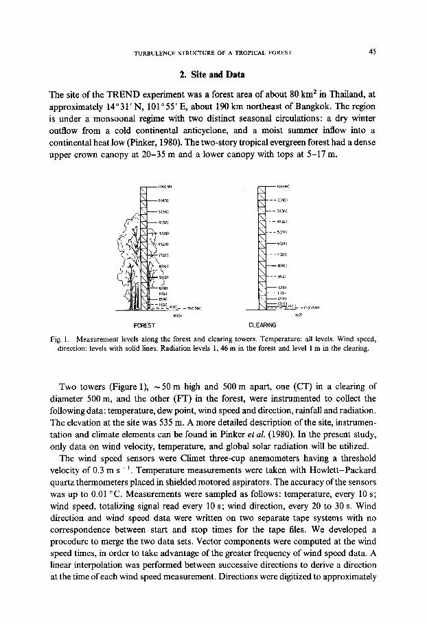
The site of the TREND experiment was a forest area of about 80 km2 in Thailand, at approximately 14”31’ N, lOl”55’ E, about 190 km northeast of Bangkok. The region is under a monsoonal regime with two distinct seasonal circulations: a dry winter outflow from a cold continental anticyclone, and a moist summer inflow into a continental heat low (Pinker, 1980). The two-story tropical evergreen forest had a dense upper crown canopy at 20-35 m and a lower canopy with tops at 5-17 m.

Fig. I. Measurement levels along the forest and clearing towers. Temperature: all levels. Wind speed, direction: levels with solid lines. Radiation levels 1, 46 m in the forest and level 1 m in the clearing.

Two towers (Figure l), - 50 m high and 500 m apart, one (CT) in a clearing of diameter 500 m, and the other (FT) in the forest, were instrumented to collect the following data: temperature, dew point, wind speed and direction, rainfall and radiation. The elevation at the site was 535 m. A more detailed description of the site, instrumentation and climate elements can be found in Pinker et al. (1980). In the present study, only data on wind velocity, temperature, and global solar radiation will be utilized.

The wind speed sensors were Climet three-cup anemometers having a threshold velocity of 0.3 m s- ‘. Temperature measurements were taken with Hewlett-Packard quartz thermometers placed in shielded motored aspirators. The accuracy of the sensors was up to 0.01 “C. Measurements were sampled as follows: temperature, every 10 s; wind speed, totalizing signal read every 10 s; wind direction, every 20 to 30 s. Wind direction and wind speed data were written on two separate tape systems with no correspondence between start and stop times for the tape files. We developed a procedure to merge the two data sets. Vector components were computed at the wind speed times, in order to take advantage of the greater frequency of wind speed data. A linear interpolation was performed between successive directions to derive a direction at the time of each wind speed measurement. Directions were digitized to approximately

46 R. T. PINKER AND J. Z. HOLLAND

0.01 radian increments and a table look-up method was used for the sine and cosine components. More details can be found in Pinker and Kaylor (1982). The radiation data used in the present study were acquired at the top of the forest tower (N 15 m above the canopy). The global shortwave radiation (0.3-3 urn) was measured by an Eppley precision pyranometer (2-junction model). An automatic data acquisition system (HP Model 7259) was used in an analog and digital mode. The radiation signals were sent to the digital voltmeter which integrated the voltage every 20 s and obtained an average value that was digitized. From this information, half-hourly averages were obtained.

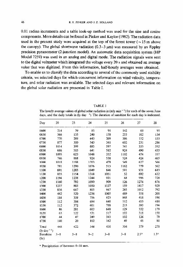
To enable us to classify the data according to several of the commonly used stability criteria, we selected days for which concurrent information on wind velocity, temperature, and solar radiation was available. The selected days and relevant information on the global solar radiation are presented in Table I.

TABLE I

The hourly average values of global solar radiation in (mly min- ‘) for each of the seven June days, and the daily totals in (ly day- I). The duration of sunshine for each day is indicated.

Day 20 23 24 25 26 2-l 28

0600 214 0630 566 0700 770 0730 817 0800 1014 0830 686 0900 1095 0930 146 1000 1018 1030 781 1100 691 1130 855 1200 1194 1230 1160 1300 1237 1330 856 1400 442 1430 184 1500 112 1530 112 1600 86 1630 63 1700 44 1730 140

Total 448

UY day - ‘) Sunshine 3-8

(hr)

39 85 135 240 289 443 300 543 399 685 505 641 023 1048 868 924

1198 1203 1290 1076 1283 1049 1154 1318 1238 1244 192 1090 883 1050 667 805 520 1236 359 756 384 694 372 601 281 603 122 431 41 249 20 102

422 546

3-8 9-2

a Precipitation of between O-10 mm.

91 158 209 341 591 582 352 538 419 515 846

1051 921 909

1527 941

1005 823 640 788 648 517 343 162

450

3-8 3-8 2.5” 1.3”

142 60 253 102 386 152 602 231 741 333 924 490

1102 414 524 424 549 627

1162 719 591 931

52 692 68 996

126 1274 159 1417 285 1012 489 558 868 416 512 453 215 393 129 332 103 318 102 126 49 45

304 319

95 134 153 286 352 433 351 465 566 562 613 632 128 676 929 192 200 196 418 194 179 150 19 81

278

TURBULENCE STRUCNRE OF A TROPICAL FOREST 41

3. Procedures and Results

3.1. PRELIMINARIES

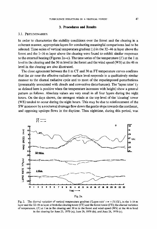
In order to characterize the stability conditions over the forest and the clearing in a coherent manner, appropriate layers for conducting meaningful comparisons had to be selected. Time series of vertical temperature gradient (y) in the 32-46 m layer above the forest and the 1-16 m layer above the clearing were found to exhibit similar responses to the external heating (Figures 2a-c). The time series of the temperature (T) at the 1 m level in the clearing and the 30 m level in the forest and the wind speed (WS) at the 46 m level in the clearing are also illustrated.

The close agreement between the 1 m CT and 30 m FT temperature curves confirms that the air near the effective radiative surface level responds in a qualitatively similar manner to the diurnal radiative cycle and to most of the superimposed perturbations (presumably associated with clouds and convective disturbances). The ‘lapse rates’ (y as defined here is positive when the temperature increases with height) show a general pattern as follows. Absolute values are very small in all four layers during the night hours. On the days shown, the strongest winds at the top level of the ‘clearing’ tower (WS) tended to occur during the night hours. This may be due to reinforcement of the SW monsoon by a nocturnal drainage flow down the gentle slope towards the northeast, and opposing upslope flows in the daytime. Thus nighttime, during this period, was

CT - FT -m-

1%

.05.

2 3

o-.. .-y __. I

e. r -.05-

F -1.1 -

2 .os- - -./ - 2

3 0. 3 .-y.Y-/. TM’

0 I 2 3 4 5 6 7 6 6 a II 12 I3 I4 I5 16 .R m I3 20 2l 22 23

TIM-

Fig. 2a.

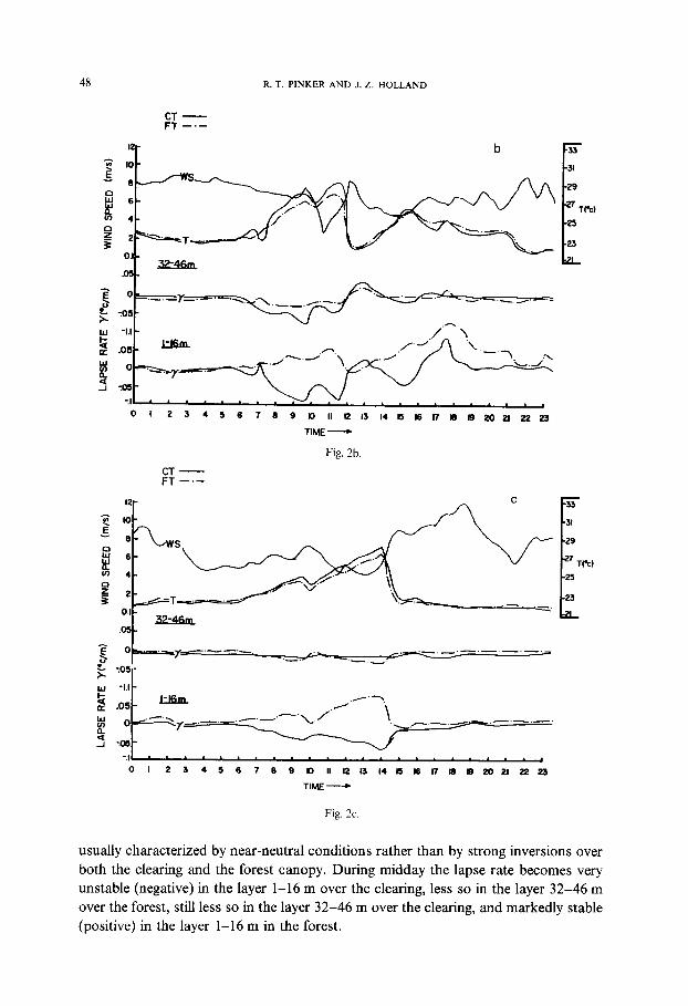
Fig. 2. The diurnal variation of vertical temperature gradient (‘Lapse rate’ y = + aT/%Z), in the 1-16 m layer and the 32-46 m layer at both the clearing tower (CT) and the forest tower (FT); the diurnal variation of temperature, (T) at 1 m in the clearing and 30 m in the forest and wind speed (WS) at the 46 m level

in the clearing for June 23, 1970 (a); June 26, 1970 (b); and June 28, 1970 (c).

R. T. PINKER AND .I. Z. HOLLAND

CT - FT -.-

0 I 2 3 4 5 6 7 6 9 D II 12 I3 14 I5 I6 I7 16 I9 20 21 22 23

TIME -

Fig. 2b.

CT - FT -.-

-2 0 3 t-

Y-.-‘-‘-‘- ,-e __- w .-._.___

k

-’ -05 -

w -1.1 L t Ll6m. ./‘Y (L .os .A % 0 I- -v .-,

Y-‘-’ .-.- .--I./ \,.-.-- .-.-.-.

% -I To5 -.lI* ’ * ’ * ’ * * *. . . . . . . . . . . . . .

0 I 23466769Dll~l3l4~l6R~B202l2223

TIME-

Fig. 2c.

usually characterized by near-neutral conditions rather than by strong inversions over both the clearing and the forest canopy. During midday the lapse rate becomes very unstable (negative) in the layer 1-16 m over the clearing, less so in the layer 32-46 m over the forest, still less so in the layer 32-46 m over the clearing, and markedly stable (positive) in the layer 1-16 m in the forest.


Disturbances indicated by sharp increases in wind speed with sharp decreases in solar radiation (Table I) and temperature occurred at about 1200 on June 26 (Figure 2b) and 1430 on June 28 (Figure 2~). On both occasions the lapse rates (y) at 1-16 m at CT and FT converged and, in the tirst case, crossed the layer within the forest becoming unstable (negative ‘lapse rate’) while at the same heights over the clearing the air became stable, as did that above the forest canopy on both occasions.

The lapse rate affects the supply of energy to turbulence. Therefore, an enhancement of turbulence by buoyancy can be expected during sunny days near the surface in the clearing and above the effective radiative surface of the forest. At the same time, the stability within the forest might tend to suppress turbulence. On the basis of these findings, the 1-16 m level above the clearing and the 32-46 m level above the forest were selected for characterizing the free air surface-layer parameters.

3.2. STABILITY CLASSIFICATION

The gradient Richardson Number (Pi) defined as:

ti = 5 am T (a2.4/az)2 (1)

was used for stability classification. The layer 1-16 m was used for the clearing tower and 32-46 m for the forest tower. Half-hourly averaged data were used to compute Pi. The range of the hourly values of Ri was divided into three intervals characterized as:

Ri < - 0.03 unstable, - 0.03 I Ri < 0.03 neutral,

Ri 2 0.03 stable.

All hourly observations were sorted into these categories. According to the Monin-Obukhov (M-O) similarity theory, assuming horizontal

homogeneity and steady state, the standard deviations of vertical and horizontal wind direction fluctuations are functions of z/z0 and z/L, where

L= - u’, c*p”

kgH . (2)

Since both z/L and Ri measure the relative importance of buoyant suppression (or production) and mechanical (shear) production of turbulence, we expect a functional relationship. Several relationships between L and Ri have been suggested. According to the Businger-Dyer-Pandolfo empirical results (Panofsky and Dutton, 1984)

for neutral cases: z/L = Ri r 0 ) (3)

for stable cases: z/L = Ri

(1.0-S Pi) ’

for unstable cases: z/L = Ri

(0.6 Ri-1.0) ’

(4)


These equations give an estimate of L. from measurements of Ri. Since U, and H are assumed independent of height in the surface boundary layer, L can also be assumed constant with height in this layer.

3.3. SITE PARAMETERS

For near-neutral conditions, it is assumed that the wind speed variation with height above the forest canopy is represented by the simplified logarithmic relation:

ii(z) = (u, /k) In [(z - d)/z,] . (6)

A value of d is assumed, then z, is estimated as the intercept of the linear regression of the mean horizontal wind speed U(z) against log(z - d) and u * is estimated from the slope.

In the present study, we used a least-square approach to estimate d. For each neutral profile, we started with a first-guess value of d = 27 m, performed a least-square fit and derived all the micrometeorological parameters. Then, d was increased by 1 m and the procedure was repeated. The d value which yielded the best least-square fit was selected and the corresponding site parameters were computed. The resulting statistics for all the parameters are presented in Table II. In our previous study (Thompson and Pinker, 1975), the more general approach of Stearns (1970) was adopted for computing z, and d. Surface roughness and displacement height were determined simultaneously so that the sum of error squares on wind speed were a minimum, namely:

q = Vi - u,k-’ In [ (“-f’“) + $j]Y

where si is the error between the measured wind speed at the different zi levels and the theoretical wind speed at the same height. The least-square method (Lettau, 1957; Robinson, 1962) requires that xr=, $ is a minimum for n measurement levels. For June, this approach yielded a value of d = 27 m. Had we adopted this latter value of d, the micrometeorological parameters would assume values as presented in Table II(b).

It has been recognized that the value chosen for d can significantly affect the other micrometeorological parameters, in particular, the flux-profile relationships and the stability functions (Raupach, 1979; Garratt, 1980). Originally, d was considered to be an empirical parameter introduced to retain the logarithmic law above tall vegetation, under neutral conditions. Later, attempts have been made to associate d with some physical properties of the atmosphere/vegetation interactions. Thorn (1971) suggested the ‘centre of pressure’ hypothesis, associating d with the mean level of momentum absorption. More recently, Molion and Moore (1983) estimated d for tall vegetation using a mass conservation method.

Similar considerations exist about the proper derivation of z, and in particular, its dependency on wind speed and wind direction. Generally, it is assumed that z. is a constant site parameter independent of the height of measurement. In irregular terrain, however, it has been suggested (Holland, 1952; Beljaars, 1982; Kaimal et4 1982;


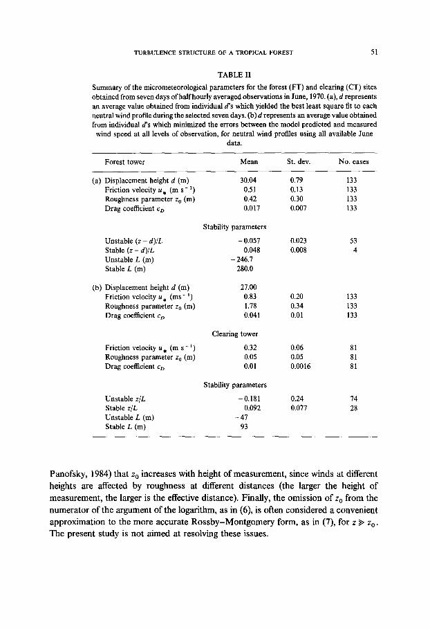
TABLE II

Summary of the micrometeorological parameters for the forest (ET) and clearing (CT) sites obtained from seven days of half hourly averaged observations in June, 1970. (a), d represents an average value obtained from individual rfs which yielded the best least square fit to each neutral wind profile during the selected seven days. (b) d represents an average value obtained from individual Ss which minimized the errors between the model predicted and measured wind speed at all levels of observation, for neutral wind profiles using all available June

data.

Forest tower Mean St. dev. No. cases

(a) Displacement height d (m) 30.04 0.79 133 Friction velocity u * (m s - ‘) 0.51 0.13 133 Roughness parameter zc (m) 0.42 0.30 133 Drag coefficient c, 0.017 0.007 133

Unstable (z - d)/L Stable (z - d)/L Unstable L (m) Stable L (m)

(b) Displacement height d (m) 27.00 Friction velocity u * (ms - ‘) 0.83 Roughness parameter z0 (m) 1.78 Drag coefficient cg 0.041

Friction velocity u + (m s - ‘) Roughness parameter z, (m) Drag coefficient c,

Unstable z/L Stable z/L Unstable L (m) Stable L (m)

Stability parameters

- 0.057 0.048

- 246.7 280.0

Clearing tower

0.32 0.05 0.01

Stability parameters

-0.181 0.092

-47 93

0.023 53 0.008 4

0.20 133 0.34 133 0.01 133

0.06 81 0.05 81 0.0016 81

0.24 74 0.077 28

Panofsky, 1984) that z, increases with height of measurement, since winds at different heights are affected by roughness at different distances (the larger the height of measurement, the larger is the effective distance). Finally, the omission of z. from the numerator of the argument of the logarithm, as in (6), is often considered a convenient approximation to the more accurate Rossby-Montgomery form, as in (7), for z $- z. . The present study is not aimed at resolving these issues.

52 R. T. PINKER AND I. Z. HOLLAND

3.4. TURBULENCE STATISTICS

3.4.1. Data Processing

The high-frequency temperature and wind velocity data were processed to derive mean hourly values of temperature (T), horizontal wind speed (7) and direction (8) and horizontal wind components (U; 5). The standard deviations (a,; a,; a,; 0,; crV) were computed from each hourly mean, using the 360 data points in each sample. The covariance terms u’T’, v’T’, u’T’, V’T’, and 8’T’ were also computed. After deriving the average wind speed and direction for each hourly sample, the wind vector for each 10 s was decomposed into along- and cross-wind components and the Q statistics for these components (a,, and crCcw) were derived as well. All the turbulence statistics products were stored on tapes for possible future analyses. Only a few of these products have been analyzed. Data quality checks were conducted on all the data used. For instance, histograms of frequency distributions of temperature, wind direction and the u and v components were constructed. It became evident that the wind direction data for the 32 m level at the forest and at the 24 m level in the clearing might be in error, for all seven days investigated. Therefore, these two levels were eliminated from further analyses involving wind direction.

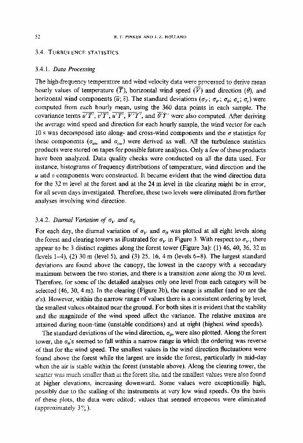
3.4.2. Diurnal Variation of cv and a,

For each day, the diurnal variation of by and a, was plotted at all eight levels along the forest and clearing towers as illustrated for I+ in Figure 3. With respect to by, there appear to be 3 distinct regimes along the forest tower (Figure 3a): (1) 46, 40, 36, 32 m (levels l-4), (2) 30 m (level 5), and (3) 25, 16, 4 m (levels 6-8). The largest standard deviations are found above the canopy, the lowest in the canopy with a secondary maximum between the two stories, and there is a transition zone along the 30 m level. Therefore, for some of the detailed analyses only one level from each category will be selected (46, 30, 4 m). In the clearing (Figure 3b), the range is smaller (and so are the O’s). However, within the narrow range of values there is a consistent ordering by level, the smallest values obtained near the ground. For both sites it is evident that the stability and the magnitude of the wind speed atfect the variance. The relative maxima are attained during noon-time (unstable conditions) and at night (highest wind speeds).

The standard deviations of the wind direction, o,, were also plotted. Along the forest tower, the 0;s seemed to fall within a narrow range in which the ordering was reverse of that for the wind speed. The smallest values in the wind direction fluctuations were found above the forest while the largest are inside the forest, particularly in mid-day when the air is stable within the forest (unstable above). Along the clearing tower, the scatter was much smaller than at the forest site, and the smallest values were also found at higher elevations, increasing downward. Some values were exceptionally high, possibly due to the stalling of the instruments at very low wind speeds. On the basis of these plots, the data were edited; values that seemed erroneous were eliminated (approximately 3 %).

TURBULENCE STRUCTURE OF A TROPICAL FOREST

AVERAGE SPEED (FT) DAY 2 3

1=46M 2=40M 3=36M 4=32M 5=30M 6=25# 7=16M 6=4M

53

2.40 r

2.16

I I / I I

b -

1.92

1.66

1.44

0.24

0.00 I I 1 I I

00 04 06 12 16 20 24

TIME (LST)

2.40 I I , I /

1

2.16 a

1.92

3 1.66

i

1.44

1.20

0.96

0.72

0.46

0.24

0.00

00 04 06 12 16 20 24

TIME iLST1

AVERAGE SPEED (CT) DAY 23

1=46M 2=32M 3=24M 4=16M 5=8M 6=4M 7=2M 8=1M

Fig. 3. (a) The diurnal variation of the wind speed standard deviation (av) for all eight (FT) levels, for June 23, 1970. (b) Same as Figure 3a for the (CT).


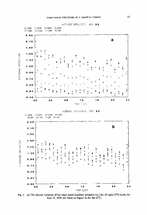
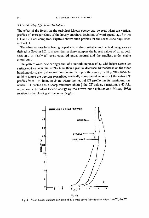
3.4.3. Stability Efects on Turbulence

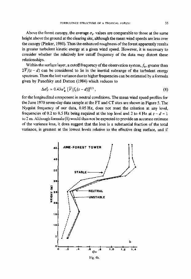
The effect of the forest on the turbulent kinetic energy can be seen when the vertical profiles of average values of the hourly standard deviation of wind speed, cry, for the CT and FT are compared. Figure 4 shows such profiles for the seven June days listed in Table I.

The observations have been grouped into stable, unstable and neutral categories as defined in Section 3.2. It is seen that in these samples the largest values of q, at both sites and at nearly all levels occurred under neutral and the smallest under stable conditions.

The pattern over the clearing is that of a smooth increase of Q, with height above the surface up to a maximum at 24-32 m, then a gradual decrease. In the forest, on the other hand, much smaller values are found up to the top of the canopy, with profiles from 32 to 46 m above the treetops resembling vertically compressed versions of the entire CT profiles from 1 to 46 m. At 24 m, where the neutral CT profile has its maximum, the neutral FT profile has a sharp minimum about i the CT values, suggesting a 40-fold reduction of turbulent kinetic energy by the crown zone (Pinker and Moses, 1982) relative to the clearing at the same height.

45

4a

36

,.

I. .

1.

I-.

i..

I.,

5”

3, 0

JUNE-CLEARING TOWER

NEUTRAL

STABLE- I’

Fig. 4a.

Fig. 4. Mean hourly standard deviation of 10 s wind speed (abscissa) vs height. (a) CT; (b) FT.

TURBULENCE STRUCNRE OF A TROPICAL FOREST 55

Above the forest canopy, the average cry values are comparable to those at the same height above the ground at the clearing site, although the mean wind speeds are less over the canopy (Pinker, 1980). Thus the enhanced roughness of the forest apparently results in greater turbulent kinetic energy at a given wind speed. However, it is necessary to consider whether the relatively low cutoff frequency of the data may distort these relationships.

Within the surface layer, a cutoff frequency of the observation system, f0 , greater than 2v/(z - d) can be considered to lie in the inertial subrange of the turbulent energy spectrum. Then the lost variance due to higher frequencies can be estimated by a formula given by Panofsky and Dutton (1984) which reduces to

Ati, = 0.43~2, [V/&(z - d)]“’ , (8)

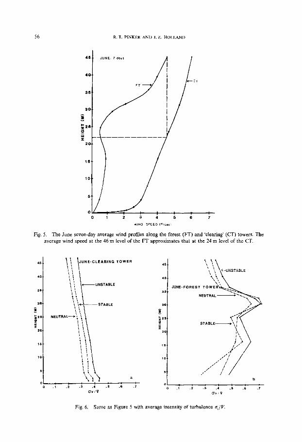
for the longitudinal component in neutral conditions. The mean wind speed profiles for the June 1970 seven-day data sample at the FT and CT sites are shown in Figure 5. The Nyquist frequency of our data, 0.05 Hz, does not meet the criterion at any level, frequencies of 0.2 to 0.5 Hz being required at the top level and 2 to 4 Hz at z - d = 1 to 2 m. Although formula (8) would thus not be expected to provide an accurate estimate of the variance loss, it does suggest that the loss is a substantial fraction of the total variance, is greatest at the lowest levels relative to the effective drag surface, and if

45.8

40.'

25.

15..

10..

5..

JUNE-FOREST TOWER t I

I’

‘4”

/

STABLE ___, / i

i i

i i i

.' 1

.d 1’

NEUTRAL

i ? I I I I I I ?

: I i

I’ .‘. : I

i 1’ ,’ I’ i

: ? I‘ ’ /

b 0

0 .2 .4 .5 .5 1.0 1.2 1.4 CT-4

Fig. 4b.

R. T. PINKER AND I. Z. HOLLAND

45

35

15

10

5

0 1

Fig. 5. The June seven-day average wind profiles along the forest (FT) and ‘clearing’ (CT) towers. The average wind speed at the 46 m level of the FT approximates that at the 24 m level of the CT.

b 0

0 .I .2 .3 .4 .5 .B .7 UV/V

Fig. 6. Same as Figure 5 with average intensity of turbulence u,/V.

JUNE-

51 TURBULENCE STRUCTURE OF A TROPICAL FOREST

2.0 -.

” .

: 1.2 -- E

: a

cn

0.4 --

N=

a FT: 32m

Neutral

2.0

” .

: 1.2

E

u 3I a

cn

0.4

0.6 2.4 4.0 5.6

WIND (m/sac)

N =I59

rz.911

c c

c

c

x CCL

.cxzeXc Eccc t

c CQttc

c c 2°C” c c c

c cc c c

F c

E c

b Cl: 6m

Neutral

0.7 2.1 3.5 4.9

WIND (m/set)

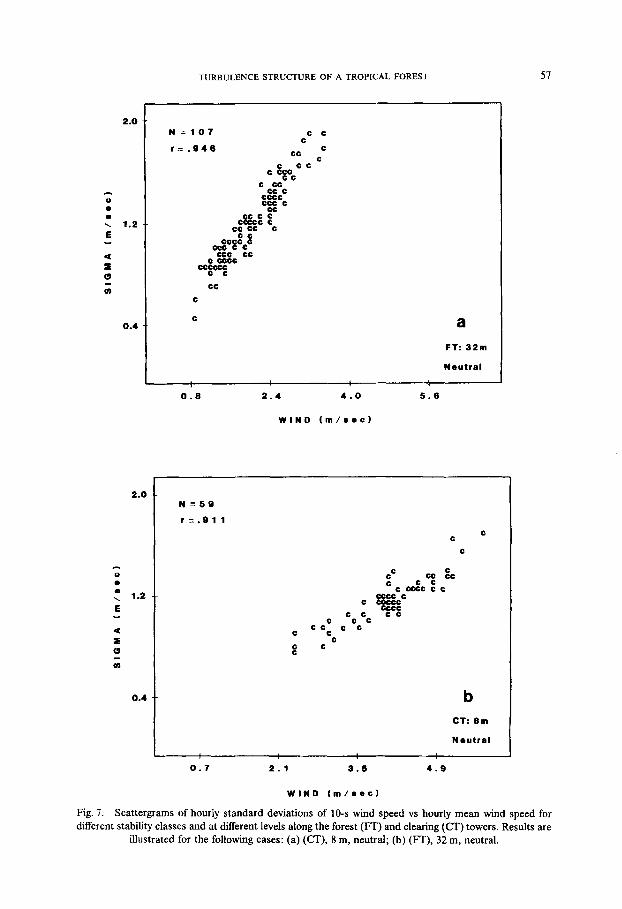
Fig. 7. Scattergrams of hourly standard deviations of 10-s wind speed vs hourly mean wind speed for different stability classes and at different levels along the forest (FT) and clearing (CT) towers. Results are

illustrated for the following cases: (a) (CT), 8 m, neutral; (b) (IT), 32 m, neutral.


corrected would decrease the vertical gradient of oy in the lowest few meters (i.e., 30 to 36 m at the forest tower, even more so 1 to 8 m over the clearing). Thus the apparent

deviation of the or, profile from constancy in the surface layer may be due in part to a height-dependent negative bias.

When the standard deviations are normalized by mean speed, the ‘intensity of turbulence’ ~,/v is obtained. Vertical profiles of this quantity are shown in Figure 6. For the CT, the values decrease smoothly and at similar rates with height for all stabilities, those for the unstable case being consistently the greatest. At the FT, the profiles for the atmospheric layer above the canopy top behave in a qualitatively similar

manner but with larger values, and a more rapid decrease with height. Below the canopy

top, however, turbulence intensities vary in a more irregular manner, generally increasing upward but apparently also reflecting varying canopy density at different levels (Pinker and Moses, 1982).

The intensities at the canopy top and within the forest are large compared to those reported by Allen (1968) in a larch plantation. They are comparable to those reported by Shaw et al. (1974) in a dense corn canopy; they are probably significantly underestimated. This would be particularly important at the canopy top. It is there that Monin-Obukhov similarity theory, confirmed by Maitani’s (1979) compilation, would predict larger intensities relative to those higher up. Also both the extensively confirmed inertial subrange spectrum as embodied in the variance correction formula (8) and the high-frequency wind observations of Allen (1968) suggest that a large fraction of the variance should be contributed by frequencies greater than 0.05 Hz in the free air layer immediately adjacent to the canopy top. Over the clearing, too, the total intensity would be expected to increase more strongly downward towards the surface if the higher frequencies were included. In the lower canopy, on the other hand, if high frequencies are suppressed as suggested by McBean (1968) and Allen (1968), the intensity values of 0.4 to 0.6 shown in Figure 7 may be realistic.

In the neutral surface layer, gr, is expected to be directly proportional to V at a given height. In each stability class, the ds were plotted as a function of wind speed at all eight levels along the forest and clearing towers. Selected results for neutral stability are illustrated in Figure 7. As evident from this figure, the standard deviations increase linearly with wind speed in neutral conditions but the slopes and degree of scatter vary according to the measurement level and environment. Correlation coefficients vary from greater than 0.9 near the clearing surface (Figure 7a) and the forest canopy top (Figure 7b) to less than 0.1 at the 46 m level over the clearing.

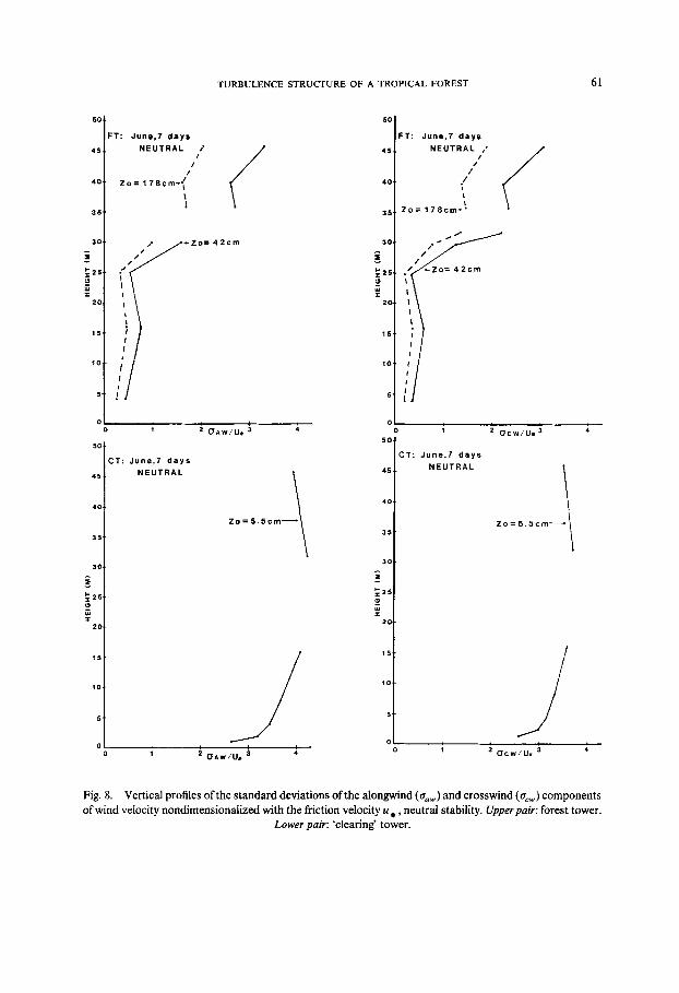
When the wind velocities for those observation levels having reliable direction measurements are decomposed into alongwind (aw) and crosswind (cw) components and the standard deviations for neutral stability conditions are divided by u *, we expect to find the ‘universal constants’ for the surface layer, as modified by upstream memory effects (Panofsky and Dutton, 1984). Profiles of these results, shown in Figure 8, bear out this expectation to some extent. Over the clearing, allowing for increasing under- estimation due to high frequency loss as the surface is approached, the values of about 4 for a,,,)/~ * and 3.5 for oJu* are close to those cited by Panofsky and Dutton (1984)

TURBULENCE STRUCKIRE OF A TROPICAL FOREST 59

for mountainous terrain. This is consistent with incomplete adjustment due to a fetch of only a few hundred meters over the clearing, with a forest surface upstream. Over the rough forest surface the values are closer to the ‘flat terrain values found elsewhere, reflecting equilibrium. The two different methods of determining d, z, , and u * (Table II) resulted in different profiles above the canopy top. The lower d (27 m), based on the more general Lettau-Stearns algorithm, was associated with a larger z,, (1.78 m) and U* (0.83 m s- ‘) giving CJ,,/U, and ocw/u, values at the 46 m level only a few percent lower than the ‘universal’ average of 2.4 and 1.9, respectively (Panofsky and Dutton, 1984). The choice of the higher d (30 m), with smaller z, (0.42 m) and U* (0.51 m s- i), based on the iterative short-cut method, resulted in values up to 30% higher.

3.4.4. Wind Direction Shear

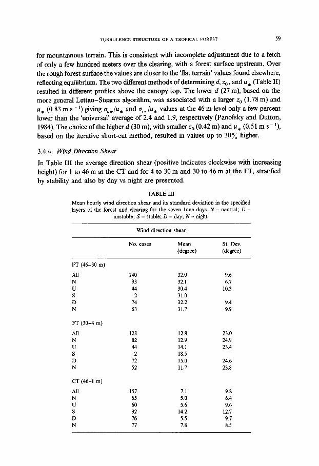
In Table III the average direction shear (positive indicates clockwise with increasing height) for 1 to 46 m at the CT and for 4 to 30 m and 30 to 46 m at the FT, stratified by stability and also by day vs night are presented.

TABLE III

Mean hourly wind direction shear and its standard deviation in the specified layers of the forest and clearing for the seven June days. N - neutral; U -

unstable; S - stable; D - day; N - night.

Wind direction shear

No. cases Mean (degree)

St. Dev. (degree)

FT(46-30 m)

All 140 32.0 N 93 32.1 U 44 30.4 S 2 31.0 D 74 32.2 N 63 31.7

FT (30-4 m)

All 128 12.8 N 82 12.9 U 44 14.1 S 2 18.5 D 72 15.0 N 52 11.7

CT (46-l m)

All 157 7.1 9.8 N 65 5.0 6.4 U 60 5.6 9.6 S 32 14.2 12.7 D 76 5.5 9.7 N 77 7.8 8.5

9.6 6.7

10.3

9.4 9.9

23.0 24.9 23.4

24.6 23.8


As shown by Smith et al. (1972), the turning of the wind above a forest canopy tzo N 1 m) from the geostrophic wind direction is considerably greater than that over a grassy field, particularly under stable conditions (35-40 “). Within the forest canopy, the turning depends upon the forest parameters as well as upon meteorological conditions, and is subject to great variability. Smith et al. (1972) predicted a direction shear of the order of 30” in a pine forest and found a mean value of 27” in 385 hr of data with a large standard deviation (20”).

Although we have not computed geostrophic winds, we find an average direction shear between the average canopy top (30 m) and the 46 m level over the forest of 32” (140 hr of data) compared with 7 ’ between the surface (1 m) and 46 m over the clearing (157 h of data), with standard deviation of 10” at both sites. Within the canopy (30-4 m), we find an additional turning of 13 ’ (128 hr of data), smaller than that found by Smith et al., but with a comparable standard deviation (23”).

The effect of stability appears to be in the expected sense at the CT. Above and within the forest, however, because of the small samples and large standard deviations, this effect can not be established with significance in the present analysis.

4. Summary

The data collected during the TREND experiment span almost a whole year and have proven to be of very high quality. They are suited to provide information on the height dependence of the horizontal wind fluctuations over and inside a tropical forest canopy, and facilitate comparison between rough and relatively smooth surfaces, under identical ambient conditions. This study presents an analysis of a sample of hourly averages and standard deviations of 10 s recordings of wind components at the TREND forest and clearing towers, in association with temperature profiles and solar radiation data.

The responses of the flow in the 16 m thick ‘free atmosphere’ layer above the 30 m average height of the forest canopy to diurnal stability variations, free-atmosphere mean wind fluctuations, and surface friction resembled those of the 46 m layer above the clearing in many ways: the wind speed profiles were approximately logarithmic in neutral stability conditions; the measured (frequency IO.05 Hz) turbulent kinetic energy increased upward, more gradually in stable (i.e., nighttime) conditions and most rapidly up to maxima within the layer in neutral (i.e., strong wind) conditions; the linear correlations between the turbulence, as represented by the standard deviation of wind speed +, and mean wind speed 7, as well as the intensity of turbulence a,/F, decreased with height, the intensity being greatest in unstable and least in neutral conditions.

The forest and clearing ‘free atmosphere’ layers differed significantly in some respects. The average stress (as represented by the friction velocity U, inferred from the wind profile), roughness length, and drag coefficient were much greater over the forest than over the clearing. Correlations of 0” with 7, linear regression slopes, and average intensities (a,/F) were much larger over the forest than over the clearing. Instability produced a more distinct enhancement of turbulent wind fluctuations over the clearing than over the forest. Average wind direction shear was much greater over the forest.


50.

FT: June,7 days

a.. NEUTRAL i I

/ I

40. zo= 178wn*(

I

4

:T: June,7 days NEUTRAL

\

Zo=5.5cm-

501

FT: June,7 days

45.. NEUTRAL ,*

/I

CT:

45

10

55

30.

3

:25 z :

20.

June,7 days NEUTRAL

Fig. 8. Vertical profiles of the standard deviations of the alongwind (u,,) and crosswind (a,,) components of wind velocity nondimensionalized with the friction velocity U* , neutral stability. Upperpair: forest tower.

Lower pair: ‘clearing’ tower.

62 R. T. PINKER AND J. 2. HOLLAND

The layer within the forest canopy exhibited a completely different flow regime from that at the clearing or that overlying the forest. The vertical temperature gradient tended to be positive (stable) during midday, and generally varied in the opposite sense to that in the ‘free atmosphere’ layers. In view of the very weak mean wind and absence of mean vertical shear within the canopy, or, was about an order of magnitude smaller, implying turbulent kinetic energy two orders of magnitude smaller, than in the clearing at the same levels. On the other hand, the intensity a,,/7 was much larger within the canopy. Clearly, the turbulence within the forest is strongly coupled with the mean wind, while buoyancy effects associated with instability cannot be seen.

The sample of data examined here has provided a self-consistent and physically plausible description of the vertical distribution of the mean wind, temperature and their turbulent fluctuations in and above the forest and over the clearing. This has enabled us to define limits for the distinguishable regimes in terms of stability and height and to design with confidence a statistical analysis program for the larger data set.

Acknowledgements

This work was supported by Grant No. DAAG29-80-C-0012 from the U.S. Army Research Office, Durham, N.C., to the University of Maryland. Our thanks are extended to the granting agency, to R. Kaylor for his continuous help with the data processing effort and to C. Burr, for his technical assistance. We are grateful to the Computer Science Center, University of Maryland, for providing supplementary computer time.

References

Allen, L. H., Jr.: 1968, ‘Turbulence and Wind Speed Spectra within a Japanese Larch Plantation’, J. Appl. Meteorol. I, 73-18.

Beljaars, A. C. M.: 1982, ‘The Derivation of Fluxes from Profiles in Perturbed Areas’, Boundary-Layer Meteorol. 24, 35-55.

Cionco, R. M.: 1965, ‘A Mathematical Model for Air Flow in a Vegetative Canopy’, J. Appl. Meteorol. 4, 517-522.

Garratt, J. R.: 1980, ‘Surface Influences upon Vertical Profiles in the Atmospheric Near-Surface Layer’, Quart. J. R. Meteorol. Sot. 106, 803-819.

Holland, J. 2.: 1952, ‘The Diffusion Problem in Hilly Terrain’, Air Pollution, Proceedings of the United States Technical Conference on Air Pollution, McGraw-Hill, New York, 815-821.

Kaimal, J. C., Eversole, R. A., Lenschow, D. H., Stankov, B. B., Kahn, P. L., and Businger, J. A.: 1982, ‘Spectral Characteristics of the Convective Boundary Layer over Uneven Terrain’, J. Atmos. Sci. 39, 1098-l 114.

Maitani, T.: 1979, ‘A Comparison of Turbulence Statistics in the Surface Layer over Plant Canopies with Those over Several Other Surfaces’, Boundary-Layer Meteorol. 17, 213-222.

McBean, G. A.: 1968, ‘An Investigation of Turbulence Within a Forest’, J. Appl. Meteorol. 7, 410-416. Molion, L. C. B. and Moore C. J.: 1983, ‘Estimating the Zero-Plane Displacement for Tall Vegetation Using

a Mass Conservation Method’, Boundary-Layer Mefeorol. 26, 115-125. Panofsky, H. A.: 1984, ‘Vertical Variation of Roughness Length at the Boulder Atmospheric Observatory’,

Boundary-Layer Meteorol. 28, 305-308.


Panofsky, H. A. and Dutton, J. A.: 1984, Atmospheric Turbulence Models and Methods for Engineering Applications, A Wiley-Interscience Publication, pp. 397.

Pinker, R. T., 1980: ‘The Microclimate of a Dry Tropical Forest’, Agric. Meteorol. 22, 249-265. Pinker, R. T, Thompson, 0. E., and Eck, T. F.: 1980, The Albedo of a Tropical Forest’, Quart. J. Roy.

Meteorol. Sot. 106, 551-558. Pinker, R. T. and Kaylor, R.: 1982, Data Reduction Summary for Project TREND (User’s Manual). Part I: ‘D’

Tapes, Publication No. 92-197, Department of Meteorology, College Park, MD 20742, pp. 116. Pinker, R. T. and Moses, J. F.: 1982, ‘On the Canopy Flow Index of a Tropical Forest’, Boundary-Layer

Meteorol. 22, 3 13-324. Raupach, M. R.: 1979, ‘Anomalies in Flux-Gradient Relationships over Forest’, Boundary-Layer Meteorol.

16,467-486. Shaw, R. H., den Hartog, G., King, K. M., and Thurtell, G. W.: 1974, ‘Measurements of Mean Wind Flow

and Three-Dimensional Turbulence Intensity Within a Mature Corn Canopy’, Agric. Meteorol. 13, 419-425.

Smith, F. G., Carson, D. J., and Oliver, H. R.: 1972, ‘Mean Wind-Direction Shear Through a Forest Canopy’, Boundary-Layer Meteorol. 3, 178-190.

Thorn, A. S.: 1971, ‘Momentum Absorption by Vegetation’, Quart. J. R. Meteorol. Sot. 97, 414-428. Thompson, 0. E. and Pinker, R. T.: 1975, ‘Wind and Temperature Profile Characteristics in a Tropical

Evergreen Forest in Thailand’, Tellus 27, 562-573.

turbulence structure of a tropical forest

Documents