tt: a program that implements predictor sort … : a program that implements predictor sort design...

United StatesDepartment ofAgriculture

Forest Service

ForestProductsLaboratory

GeneralTechnicalReportFPL-GTR-101

TT: A Program ThatImplements PredictorSort Design andAnalysisSteve P. VerrillDavid W. GreenVictoria L. Herian

AbstractIn studies on wood strength, researchers sometimes replaceexperimental unit allocation via random sampling withallocation via sorts based on nondestructive measurements ofstrength predictors such as modulus of elasticity and specificgravity. This report documents TT, a computer program thatimplements recently published methods to increase thesensitivity of such “predictor sort” experiments. The reportconsists of annotated keyboard sessions and computer outputfrom runs of TT.

Keywords: program, wood, nondestructive, predictor, sorting

September 1997

Verrill, Steve P.; Green, David W.; Herian, Victoria L. 1997. TT: Aprogram that implements predictor sort design and analysis. Gen. Tech.Rep. FPL-GTR-101. Madison, WI: U.S. Department of Agriculture, ForestService, Forest Products Laboratory. 21 p.

A limited number of free copies of this publication are available to thepublic from the Forest Products Laboratory, One Gifford Pinchot Drive,Madison, WI 53705-2398. Laboratory publications are sent to hundreds oflibraries in the United States and elsewhere.

The Forest Products Laboratory is maintained in cooperation with theUniversity of Wisconsin.

The use of trade or firm names is for information only and does not implyendorsement by the U.S. Department of Agriculture of any product orservice.

The United States Department of Agriculture (USDA) prohibits discrimi-nation in its programs on the basis of race, color, national origin, sex,religion, age, disability, political beliefs, and marital or familial status. (Notall prohibited bases apply to all programs.) Persons with disabilities whorequire alternative means for communication of program information(braille, large print, audiotape, etc.) should contact the USDA’s TARGETCenter at (202) 720-2600 (voice and TDD). To file a complaint, write theSecretary of Agriculture, U.S. Department of Agriculture, Washington,DC 20250, or call l-800-245-6340 (voice), or (202) 720-1127 (TDD).USDA is an equal employment opportunity employer.

TT : A Program That ImplementsPredictor Sort Design And Analysis

Steve P. Verrill, Mathematical StatisticianDavid W. Green, Supervisory Research General EngineerVictoria L. Herian, Statistician

Introduction

TT is a computer program that implements the methods developed in Verrill and Green (1996).Currently, it is available in Solaris 1.x, Solaris 2.x, and DOS versions. The program can be obtainedby sending a floppy disk to the authors, by e-mail, or via the World Wide Web’. The program canalso be run over the Web at http://wwwl.fpl.fs.fed.us/ttweb.html.

We encourage you to run the program over the Web rather than on your computer. The Webversion will always be up-to-date, you won’t encounter out-of-memory errors, and the user interfaceis better.

To run TT on a PC, you need the DOS executable files tt .exe and dosxmsf.exe. Thesefiles are included with the test files analysis.dat, testpr6.dat, and testpr20.dat in a pkzipself-extracting archive, ttzip.exe. After you have obtained ttzip.exe, create a TT directory(e.g., mkdir c: \ttdir) and place ttzip.exe in that directory. Then, while in the directory, typettzip, and the ttzip.exe archive will unpack itself. To run the TT program, you then simplytype tt while in the TT directory. Alternatively, if you place the TT directory in your PC’s pathstatement, you can run the program from anywhere in the directory tree.

This report walks you through the use of the program. It contains three sections: sample sizecalculations, specimen allocation, and analysis. The report consists of annotated keyboard sessionsand computer output. Material printed by the program is flush left and set in typewriter font.Material that you need to type is indented, set in bold type, and followed by <Return> (to indicatethe Return or Enter key). Annotations are set in italics. If you encounter difficulties in the courseof running the program and cannot resolve them through a careful reading of this document, feelfree to contact Steve Verrill at 608-231-9375 or by e-mail.

Sample Size Calculations

Sample Size Calculations: Simple – one factor, two levels

To begin the program, type tt:

t t <Return>

What name do you want for your results file?

1Steve Verrill, USDA Forest Service Forest Products Laboratory, One Gifford Pinchot Drive, Madison, WI [email protected]://www1.fpl.fs.fed.us/papers.html

WARNING!!!Any material that is currently in this file will be lost.WARNING!!!

myresult <Return>

What do you want to do?

choose a sample size - 0allocate specimens - 1analyze results - 2

0 <Return>

What kind of experiment is it?

simple experiment, 1 factor, 2 levels - - - 0complex experiment, multiple factors, multiple levels --- 1

If you ignored the predictor sort nature of your experiment, you would use a standard t testto analyze the results of a simple experiment, and a standard analysis of variance to analyze theresults of a complex experiment.

0 <Return>

This program will not tell you what sample size to use. Instead, you must give itinformation on the sizes of the differences that you want to be able to detect, onthe variability of the response (e.g., modulus of rupture (MOR)), on the correlationbetween the predictor (e.g., modulus of elasticity (MOE)) and the response, on thesignificance level that you want to achieve, and on the sample sizes that you are consid-ering.

Given this information, the program will calculate the probabilities that you willbe able to detect the differences in which you are interested (power). If these prob-abilities are too low (say below .90), then you will have to find a predictor thatis more correlated with the response, accept a larger significance level (say .10 ra-ther than .05), accept a higher risk of not statistically detecting the differencesin which you are interested, or be willing to consider larger sample sizes.

How many mean differences ( d i f f ) do you want to consider? (5 or fewer)

5 <Return>

What are the differences? (for example, .10 for a 10% difference in means)

2

.05 .1 .2 .3 .5 <Return>

How many coefficients of variation (CV) do you want to consider? (5 or fewer)(The coefficent of variation of a property is 100 × (standard deviation)/mean.)

5 <Return>

What are the CVs? (for example, .20 for a 20% coefficient of variation)

.05 .1 .15 .2 .25 <Return>

What will be the significance level of your tests?

.10 - 1

.05 - 2

.01 - 3

2 <Return>

How many sample sizes do you want to consider? (5 or fewer)

3 <Return>

What are the sample sizes? (for example, 10 if you want 10 replicates for EACH treat-ment)

5 15 25 <Return>

What is the correlation value? (between -.99 and .99)

.7 <Return>

What power calculation approach do you want to take?

To use the power tables, the significance level must be .01 or .05. Also, the diff/CVratio must lie between 0.0 and 3.0, and the number of replicates per treatment mustlie between 2 and 7, or the diff/CV ratio must lie between 0.0 and 1.5, and the numberof replicates per treatment must lie between 6 and 48. Otherwise, you cannot interpo-late within the tables.

If the tables cannot be used, a non-central T approach is automatically taken.

table/paired --- 1table/pooled --- 2table/ANOCOV --- 3non-central T --- 4

3

2 <Return>

The material below appears in the output file:

The correlation value is 0.70.

The number of replications for each treatment is 5.

Differences are on top. Coefficients of variation are along the left side. Powervalues are in the table.

0.050 0.100 0.200 0.300 0.500

0.050 0.470 0.960 1.000* 1.000* 1.000*0.100 0.160 0.470 0.960 1.000 1.000*0.150 0.101 0.261 0.709 0.960 1.000*0.200 0.080 0.160 0.470 0.800 0.9900.250 0.070 0.122 0.344 0.622 0.960

A number followed by a * indicates a value that was obtained using a non-central Tapproach rather than a power table. This approach overestimates power for correla-tions greater than .8 and small sample sizes (e.g., 6 or fewer replicates). See Ver-rill and Green’s 1996 paper for details.

The .261 entry in row 3 and column 3 of the table indicates that if we had 5 replicates for eachof the two treatments, the coefficient of variation were 15% (the standard deviation were 15% ofthe mean), and the difference between the two treatments were 10% of the mean (for example, onetreatment yielded a .95 response and the other yielded a 1.05 response), then we would have only a26% chance of detecting that difference at a .05 significance level. From the following two tables,we see that we can up this chance to 68% by using 15 replicates per treatment, and to 88% by using25 replicates per treatment.



0.050 0.100 0.200 0.300 0.500

0.050 0.944 1. 000* 1. 000* 1. 000* 1. 000*0.100 0.440 0.944 1. 000* 1. 000* 1. 000*

4

0.150 0.243 0.675 0.998 1.000* 1. 000*0.200 0.150 0.440 0.944 1.000 1. 000*0.250 0.115 0.320 0.813 0.986 1. 000*




0.050 0.100 0.200 0.300 0.500

0.050 1.000 1.000* 1.000* 1.000* 1. 000*0.100 0.668 1.000 1.000* 1.000* 1. 000*0.150 0.388 0.878 1.000 1.000* 1. 000*0.200 0.219 0.668 1.000 1.000 1. 000*0.250 0.163 0.509 0.961 1.000 1. 000*


Back to the conversation between the computer and the user:

Another power calculation approach? no - 0 yes - 1

0 <Return>

A different correlation value? no - 0 yes - 1

0 <Return>

Altered differences, CVs, and sample sizes? no - 0 yes - 1

0 <Return>

The program terminates.

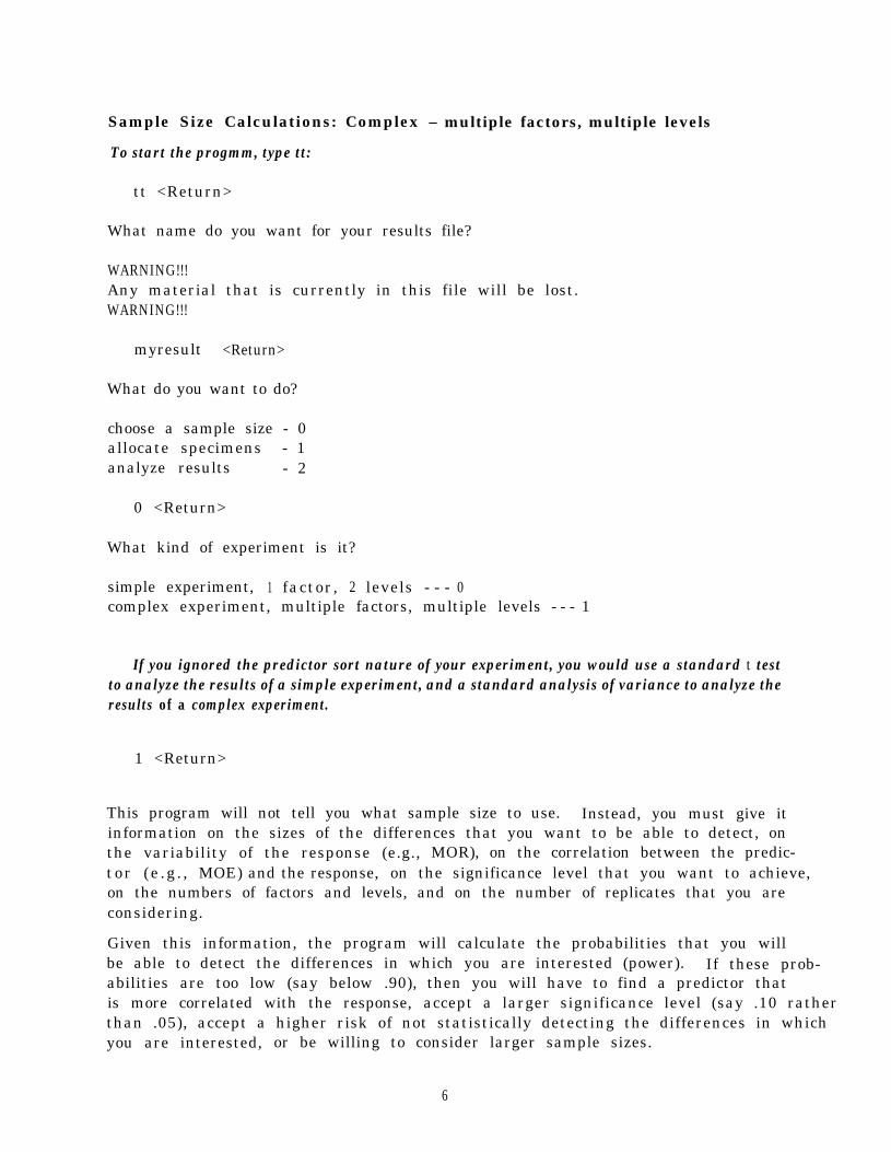
Sample Size Calculations: Complex – multiple factors, multiple levels

To start the progmm, type tt:

tt <Return>



myresult <Return>



0 <Return>


simple experiment, 1 factor, 2 levels - - - 0complex experiment, multiple factors, multiple levels - - - 1

If you ignored the predictor sort nature of your experiment, you would use a standard t testto analyze the results of a simple experiment, and a standard analysis of variance to analyze theresults of a complex experiment.

1 <Return>

This program will not tell you what sample size to use. Instead, you must give itinformation on the sizes of the differences that you want to be able to detect, onthe variability of the response (e.g., MOR), on the correlation between the predic-tor (e .g . , MOE) and the response, on the significance level that you want to achieve,on the numbers of factors and levels, and on the number of replicates that you areconsidering.

Given this information, the program will calculate the probabilities that you willbe able to detect the differences in which you are interested (power). If these prob-abilities are too low (say below .90), then you will have to find a predictor thatis more correlated with the response, accept a larger significance level (say .10 ratherthan .05), accept a higher risk of not statistically detecting the differences in whichyou are interested, or be willing to consider larger sample sizes.

6

NOTE: IF THE NUMBER OF REPLICATES IS SMALL, THEN THESE POWER CALCULATIONS WILL OVER-ESTIMATE THE POWER (AND THUS UNDERESTIMATE THE REQUIRED SAMPLE SIZE) UNLESS THE DATAIS ANALYZED VIA AN ANALYSIS OF COVARIANCE.

Do you already have values of the predictor (e.g., MOE) for all of your specimens?

no - 0yes - 1

1 <Return>

What is the name of your data file? (It must contain two columns of data. The firstcolumn must contain specimen IDS. The IDS must not contain blanks. Only the first20 characters of the IDS are retained. There must be at least one space between thetwo columns. The second column must contain the predictor values for the specimens.There may be no more than 5000 specimens.)

testpr6.dat <Return>

How many factors are there? (5 or fewer) (e.g., 3 for a three-way ANOVA)

3 <Return>

How many levels are there? (e.g., 3 2 2 for a 3x2x2 ANOVA) (There must be a totalof 25 or fewer levels.)

3 2 2 <Return>

How many replicates are there per "cell"? (e.g., to have 5 replicates in a 3x2x2 ANOVA,a total of 5x3x2x2 specimens would be required. Since the program can handle at most5000 specimens, given your proposed design, there must be 416 or fewer replicates perc e l l . )

2 <Return>

What is the starting value for the random number generator? (a positive integer lessthan 1000000000)

The “random” numbers that are generated are exactly determined by the starting value, Thus,if you want a different set of “random” numbers you must supply a different starting value.

86777 <Return>

The factors and the corresponding numbers of levels are given below. For tests ofwhich factor do you want to estimate power values?

factor number of levels1 32 23 2

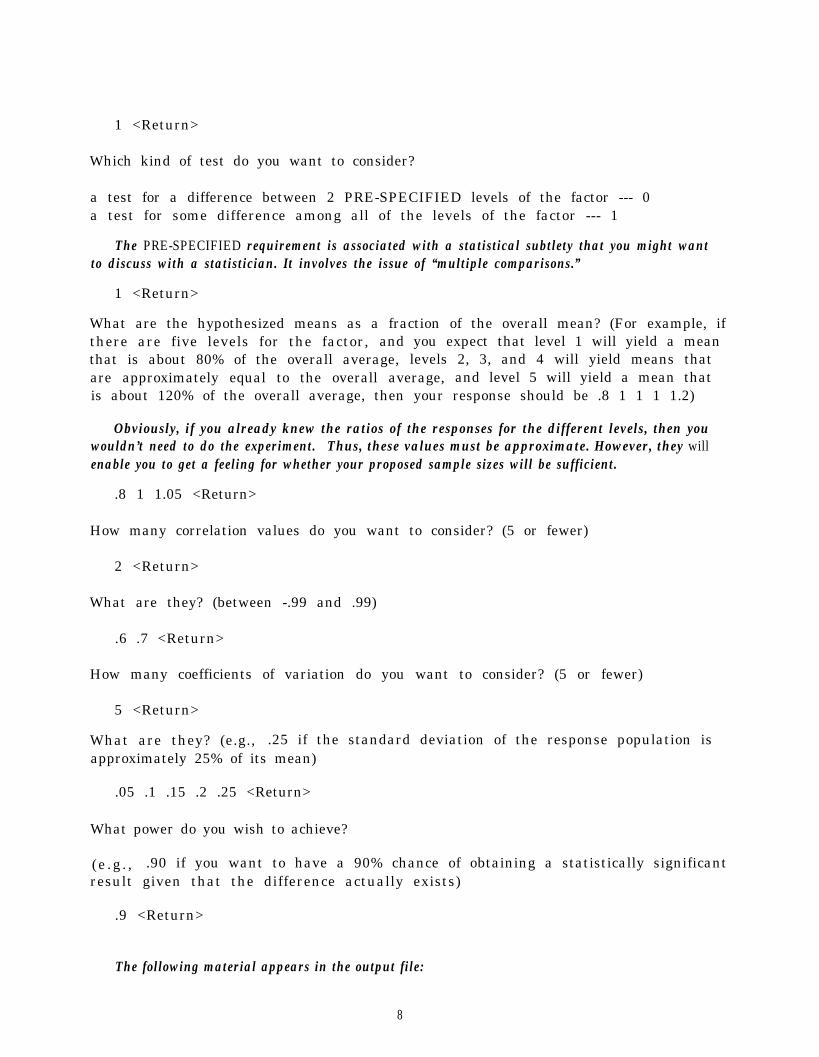
1 <Return>

Which kind of test do you want to consider?

a test for a difference between 2 PRE-SPECIFIED levels of the factor --- 0a test for some difference among all of the levels of the factor --- 1

The PRE-SPECIFIED requirement is associated with a statistical subtlety that you might wantto discuss with a statistician. It involves the issue of “multiple comparisons.”

1 <Return>

What are the hypothesized means as a fraction of the overall mean? (For example, ifthere are five levels for the factor, and you expect that level 1 will yield a meanthat is about 80% of the overall average, levels 2, 3, and 4 will yield means thatare approximately equal to the overall average, and level 5 will yield a mean thatis about 120% of the overall average, then your response should be .8 1 1 1 1.2)

Obviously, if you already knew the ratios of the responses for the different levels, then youwouldn’t need to do the experiment. Thus, these values must be approximate. However, they willenable you to get a feeling for whether your proposed sample sizes will be sufficient.

.8 1 1.05 <Return>

How many correlation values do you want to consider? (5 or fewer)

2 <Return>

What are they? (between -.99 and .99)

.6 .7 <Return>

How many coefficients of variation do you want to consider? (5 or fewer)

5 <Return>

What are they? (e.g., .25 if the standard deviation of the response population isapproximately 25% of its mean)

.05 .1 .15 .2 .25 <Return>

What power do you wish to achieve?

(e .g . , .90 if you want to have a 90% chance of obtaining a statistically significantresult given that the difference actually exists)

.9 <Return>

The following material appears in the output file:

8

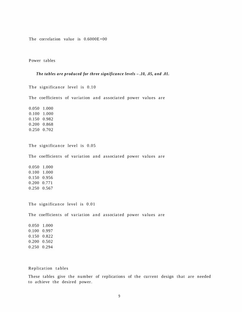
The correlation value is 0.6000E+00

Power tables

The tables are produced for three significance levels – .10, .05, and .01.

The significance level is 0.10

The coefficients of variation and associated power values are

0.050 1.0000.100 1.0000.150 0.9820.200 0.8680.250 0.702



0.050 1.0000.100 1.0000.150 0.9560.200 0.7710.250 0.567



0.050 1.0000.100 0.9970.150 0.8220.200 0.5020.250 0.294

Replication tables

These tables give the number of replications of the current design that are neededto achieve the desired power.

9

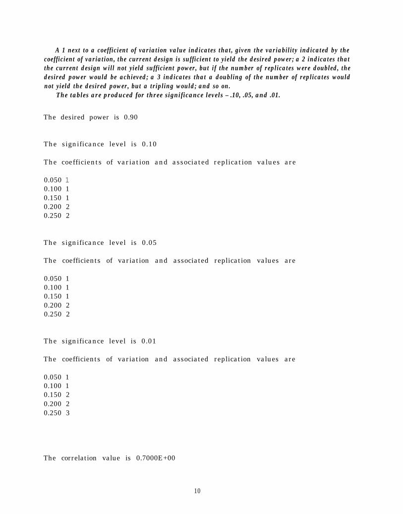
A 1 next to a coefficient of variation value indicates that, given the variability indicated by thecoefficient of variation, the current design is sufficient to yield the desired power; a 2 indicates thatthe current design will not yield sufficient power, but if the number of replicates were doubled, thedesired power would be achieved; a 3 indicates that a doubling of the number of replicates wouldnot yield the desired power, but a tripling would; and so on.

The tables are produced for three significance levels – .10, .05, and .01.

The desired power is 0.90


The coefficients of variation and associated replication values are

0.050 10.100 10.150 10.200 20.250 2



0.050 10.100 10.150 10.200 20.250 2



0.050 10.100 10.150 20.200 20.250 3

The correlation value is 0.7000E+00

10

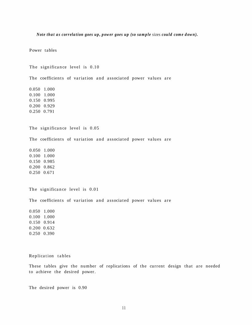
Note that as correlation goes up, power goes up (so sample sizes could come down).

Power tables



0.050 1.0000.100 1.0000.150 0.9950.200 0.9290.250 0.791



0.050 1.0000.100 1.0000.150 0.9850.200 0.8620.250 0.671



0.050 1.0000.100 1.0000.150 0.9140.200 0.6320.250 0.390

Replication tables

These tables give the number of replications of the current design that are neededto achieve the desired power.

The desired power is 0.90

11



0.050 10.100 10.150 10.200 10.250 2



0.050 10.100 10.150 10.200 20.250 2



0.050 10.100 10.150 10.200 20.250 3

Back to the conversation between the computer and the user:

Would you like to perform additional calculations based on altered sample sizes, cor-relations, CVs, etc.? no - 0 yes - 1

0 <Return>


S p e c i m e n A l l o c a t i o n

Given the values of a predictor, the program will perform the predictor sort allocation for you.

12

Specimen Allocation: Simple – one factor, two levels

To start the program, type tt:

tt <Return>



myresult <Return>



1 <Return>


simple experiment, 1 factor, 2 levels - - - 0complex experiment, multiple factors, multiple levels --- 1

0 <Return>



Here is a listing of the testpr20.dat data file. The first column contains a specimen ID. TheseIDS must not contain blanks, and, of course, they need to be distinct. For this example the secondcolumn was randomly generated from a normal distribution with mean 0 and standard deviation 1.However, in general, it would contain measured values of some predictor (e.g., MOE).

1 -0.125282 0.128973 0.884994 -0.322075 0.87034

13

6 -0.023327 -1.050398 0.450959 -1.62132

10 -0.4916511 0.0495812 -0.5015613 -0.9961014 -0.3450615 1.2927616 -1.8292817 1.1177318 0.5990319 -0.1067720 -1.23812

End of the data file.

How many replicates are there per treatment? (Since the program can handle at most5000 specimens, there must be 2500 or fewer replicates per treatment.)

10 <Return>

What is the starting value for the random number generator? (It must be a positiveinteger less than 1000000000.)

The “random” numbers that are generated are exactly determined by the starting value. Thus,if you want a different set of “random” numbers, you must supply a different starting value.

3344256 <Return>

Do you want to name the treatments? no - 0 yes - 1

1 <Return>

What are the names of the two treatments? You must type one name per line, and thenames may contain no more than 10 characters.

himom1 <Return>himom2 <Return>



The ID of the specimen, the predictor value, and the treatment are

14

1 -0.125283+00 himom22 0.128973+00 himom13 0.88499E+00 himom14 -0.322073+00 himom15 0.87033E+00 himom26 -0.233166-01 himom17 -0.l0504E+0l himom28 0.45095E+00 himom29 -0.16213E+01 himom1

10 -0.49165E+00 himom211 0.495833-01 himom212 -0.50156E+00 himom213 -0.99610E+00 himom114 -0.34506E+00 himom115 0.129283+01 himom216 -0.182933+01 himom217 0.11177E+0l himom118 0.59903E+00 himom119 -0.10677E+00 himom220 -0.123813+01 himom1

As is required, the program splits the two lowest predictor values (specimens 9 and 16) betweenthe two groups. Similarly, the two highest predictor values (specimens 15 and 17) are split betweenthe two groups, And so on.

The allocation is presented in two equivalent forms: Given a specimen, what is the treatment?Given a treatment, what are the specimens?

In addition, a third table is provided that would be useful if you wanted to use this program toanalyze the resulting data via an analysis of covariance.

The ID of the predictor block, the ID of the treatment, the ID of the specimen, andthe predictor value are

1 himom11 himom22 himom12 himom23 himom13 himom24 himom14 himom25 himom15 himom26 himom16 himom27 himom17 himom2

9 -0.l6213E+0116 -0.18293E+0120 -0.12381E+01

7 -0.10504E+0113 -0.99610E+0012 -0.50156E+0014 -0.34506E+0010 -0.49165E+004 -0.32207E+001 -0.12528E+006 -0.23316E-01

19 -0.l0677E+002 0.l2897E+00

11 0.49583E-01

15

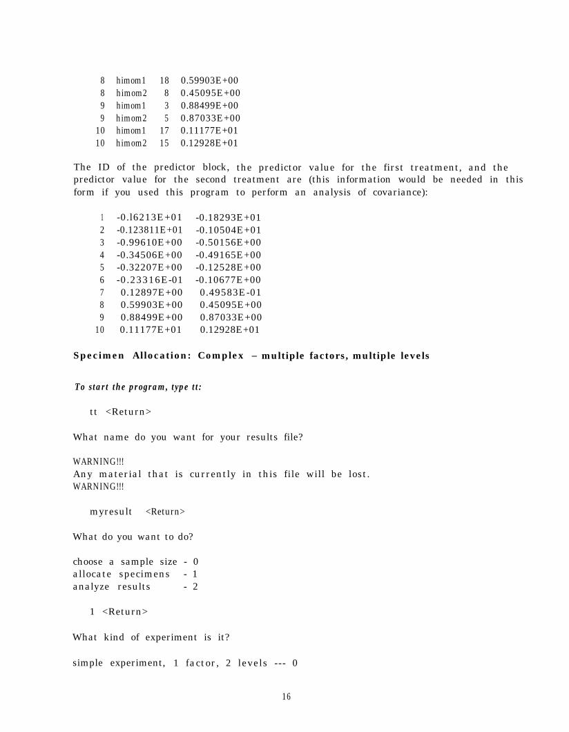
8 himom1 18 0.59903E+008 himom2 8 0.45095E+009 himom1 3 0.88499E+009 himom2 5 0.87033E+00

10 himom1 17 0.11177E+0110 himom2 15 0.12928E+01

The ID of the predictor block, the predictor value for the first treatment, and thepredictor value for the second treatment are (this information would be needed in thisform if you used this program to perform an analysis of covariance):

1 -0.l6213E+012 -0.123811E+013 -0.99610E+004 -0.34506E+005 -0.32207E+006 -0.23316E-017 0.12897E+008 0.59903E+009 0.88499E+00

10 0.11177E+01

-0.18293E+01-0.10504E+01-0.50156E+00-0.49165E+00-0.12528E+00-0.10677E+000.49583E-010.45095E+000.87033E+000.12928E+01

Specimen Allocation: Complex – multiple factors, multiple levels


tt <Return>



myresult <Return>



1 <Return>


simple experiment, 1 factor, 2 levels --- 0

16

complex experiment, multiple factors, multiple levels --- 1

1 <Return>



How many factors are there? (5 or fewer) (e.g., 3 for a three-way ANOVA)

3 <Return>

How many levels are there? (e.g., 3 2 2 for a 3x2x2 ANOVA) (There must be a totalof 25 or fewer levels.)

3 2 2 <Return>

Do you want to name the levels? no - 0 yes - 1

1 <Return>

What are the names of the 3 levels of factor 1? You must type one name per line, andthe names may contain no more than 10 characters.

small <Return>medium <Return>large <Return>


cold <Return>hot <Return>


wet <Return>dry <Return>

How many replicates are there per "cell"? (e.g., to have 5 replicates in a 3x2x2 ANOVA,a total of 5x3x2x2 specimens would be required.) (Since the program can handle atmost 5000 specimens, given your proposed design, there must be 416 or fewer repli-cates per cell.)

2 <Return>

17

What is the starting value for the random number generator? (a positive integer lessthan 1000000000)

The “random” numbers that are generated are exactly determined by the starting value. Thus,if you want a different set of “random” numbers you must supply a different starting value.

432567 <Return>


The allocation is presented in two equivalent forms: Given a “treatment,” what is the specimen?Given a specimen, what is the “treatment?”

Note that there are 3x2x2 specimens per “block” and only two blocks. For the large sampletheory described in Verrill and Green (1996) to apply, more replicates are needed. Thus, in thiscase, the data should be analyzed as a blocked analysis of variance, or, if the relationship betweenthe predictor and the response is linear, as an analysis of covariance. Commercial programs toperform the necessary analyses are widely available.


The ID of the predictor block, the levels of the factors, the ID of the specimen, andthe predictor value are

1 small1 small1 small1 small1 medium1 medium1 medium1 medium1 large1 large1 large1 large2 small2 small2 small2 small2 medium2 medium2 medium2 medium2 large2 large2 large2 large

cold wet 119 -0.10677E+00cold dry 17 -0.10504E+01hot wet 121 -0.99060E+00hot dry 19 -0.l6213E+0lcold wet 114 -0.34506E+00cold dry 112 -0.50156E+00hot wet 110 -0.49165E+00hot dry 14 -0.32207E+00cold wet 113 -0.99610E+00cold dry 116 -0.18293E+01hot wet 11 -0.12528E+00hot dry 120 -0.12381E+01cold wet 111 0.49583E-01cold dry 123 0.99494E+00hot wet 122 -0.70177E-01hot dry 13 0.88499E+00cold wet 118 0.59903E+00cold dry 16 -0.23316E-01hot wet 15 0.87033E+00hot dry 117 0.11177E+01cold wet 18 0.45095E+00cold dry 115 0.l2928E+01hot wet 12 0.12897E+00hot dry 124 -0.93164E-01

18

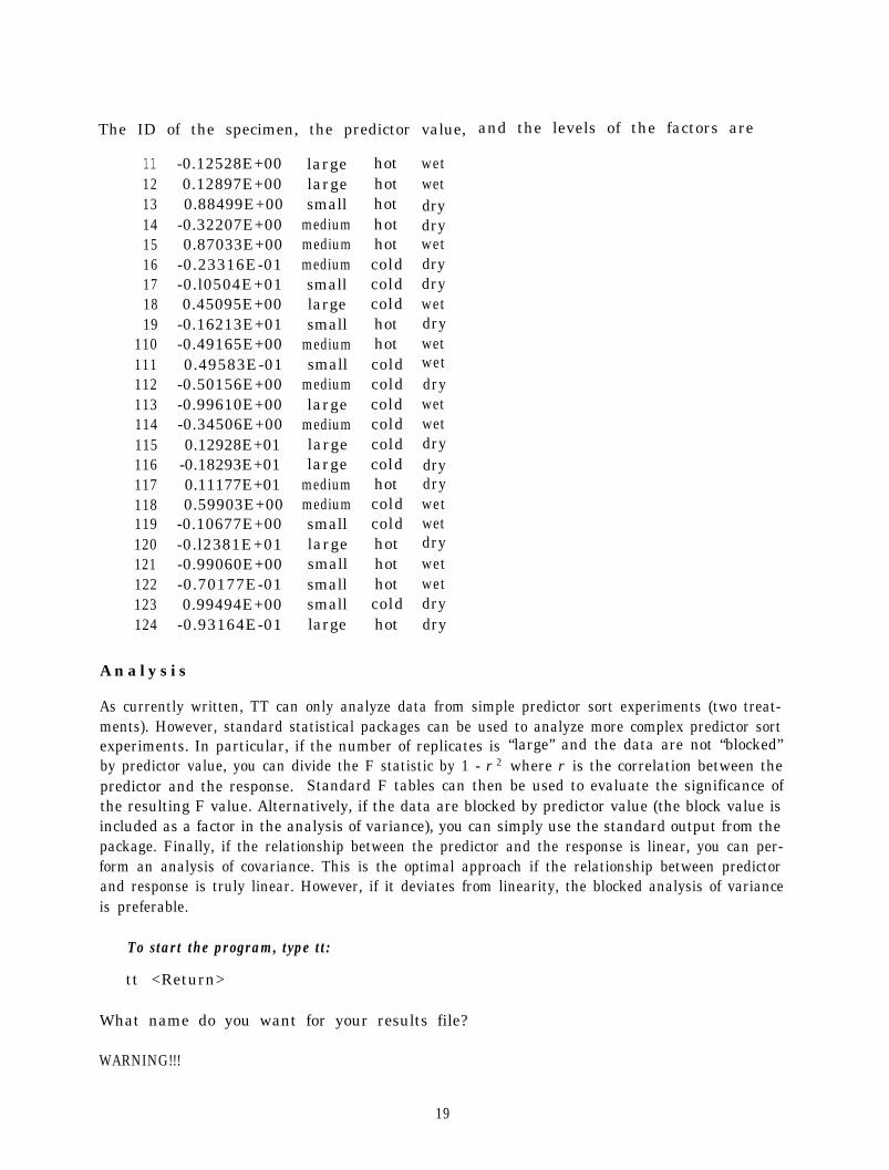
The ID of the specimen, the predictor value, and the levels of the factors are

11 -0.12528E+0012 0.12897E+0013 0.88499E+0014 -0.32207E+0015 0.87033E+0016 -0.23316E-0117 -0.l0504E+0118 0.45095E+0019 -0.16213E+01

110 -0.49165E+00111 0.49583E-01112 -0.50156E+00113 -0.99610E+00114 -0.34506E+00115 0.12928E+01116 -0.18293E+01117 0.11177E+01118 0.59903E+00119 -0.10677E+00120 -0.l2381E+01121 -0.99060E+00122 -0.70177E-01123 0.99494E+00124 -0.93164E-01

large hot wetlarge hot wetsmall hot dry

medium hot drymedium hot wetmedium cold drysmall cold drylarge cold wetsmall hot dry

medium hot wetsmall cold wet

medium cold drylarge cold wet

medium cold wetlarge cold drylarge cold dry

medium hot drymedium cold wetsmall cold wetlarge hot drysmall hot wetsmall hot wetsmall cold drylarge hot dry

A n a l y s i s

As currently written, TT can only analyze data from simple predictor sort experiments (two treat-ments). However, standard statistical packages can be used to analyze more complex predictor sortexperiments. In particular, if the number of replicates is “large” and the data are not “blocked”by predictor value, you can divide the F statistic by 1 - ρ 2 where ρ is the correlation between thepredictor and the response. Standard F tables can then be used to evaluate the significance ofthe resulting F value. Alternatively, if the data are blocked by predictor value (the block value isincluded as a factor in the analysis of variance), you can simply use the standard output from thepackage. Finally, if the relationship between the predictor and the response is linear, you can per-form an analysis of covariance. This is the optimal approach if the relationship between predictorand response is truly linear. However, if it deviates from linearity, the blocked analysis of varianceis preferable.


tt <Return>


WARNING!!!

19

Any material that is currently in this file will be lost.WARNING!!!

myresult <Return>



2 <Return>

This program will only analyze simple l-factor, 2-level experiments. If your experimentis more complex, you need to use an analysis of variance package. See Verrill andGreen’s 1996 paper for details.

Continue with the analysis? no - 0 yes - 1

1 <Return>

What is the name of your data file?

(The first column must contain the response values for treatment 1. The second columnmust contain the matched response values for treatment 2. If you want to perform ananalysis of covariance, you must also include two additional columns. The third columnmust contain the predictor values associated with the column one response values. Thefourth column must contain the predictor values associated with the column two responsevalues. There can be at most 2500 pairs of observations.)

analysis.dat <Return>

This is the data set described in section 3 of Verrill and Green (1996). It is listed in Table 56of that paper.

Does the file include the predictor value data? no - 0 yes - 1

1 <Return>

Are you just interested in the analysis of covariance results? no - 0 yes - 1

0 <Return>

How do you want the correlation to be determined?

from the data - 0experience - 1

20

(If the correlation is less than .95 and it is known from experience to within .05or .10, there should be no problem. Alternatively, if the correlation is less than.95 and the number of replicates per treatment is at least 6, the correlation can besuccessfully estimated from the data. If neither of these conditions holds, then apaired tight t or an analysis of covariance approach should be taken rather than apooled tight t approach.)

0 <Return>

The estimated correlation is 0.7220E+00.

The paired tight t value is 0.3612E+01.There are 45 replicates.The (two-sided) p value is less than .01.

The pooled tight t value is 0.2991E+01.There are 45 replicates.The (two-sided) p value is less than .01.

The analysis of covariance t value is 0.3030E+01.There are 45 replicates.The (two-sided) p value is 0.3224E-02.


Reference

Verrill, S. and Green, D. (1996). Predictor sort sampling, tight t’s, and the analysis of covariance:theory, tables, and examples. Research Paper FPL-RP-558. U.S. Department of AgricultureForest Service Forest Products Laboratory, Madison, Wisconsin.

A c k n o w l e d g m e n t s

The authors would like to express their deep appreciation to Dr. Mark Durst of the LawrenceBerkeley Laboratory, and to Dr. Jerry Winandy and Mr. Rusty Dramm of the Forest ProductsLaboratory for evaluating the TT computer program. Their many valuable suggestions greatlyimproved the final product.

21

tt: a program that implements predictor sort … : a program that implements predictor sort design...

Documents