tsp – infrastructure for the traveling salesperson problem

TSP – Infrastructure for the Traveling Salesperson

Problem

Michael Hahsler

Southern Methodist UniversityKurt Hornik

Wirtschaftsuniversitat Wien

Abstract

The traveling salesperson problem (also known as traveling salesman problem or TSP)is a well known and important combinatorial optimization problem. The goal is to findthe shortest tour that visits each city in a given list exactly once and then returns tothe starting city. Despite this simple problem statement, solving the TSP is difficultsince it belongs to the class of NP-complete problems. The importance of the TSP arisesbesides from its theoretical appeal from the variety of its applications. Typical applicationsin operations research include vehicle routing, computer wiring, cutting wallpaper andjob sequencing. The main application in statistics is combinatorial data analysis, e.g.,reordering rows and columns of data matrices or identifying clusters. In this paper weintroduce the R package TSP which provides a basic infrastructure for handling and solvingthe traveling salesperson problem. The package features S3 classes for specifying a TSPand its (possibly optimal) solution as well as several heuristics to find good solutions. Inaddition, it provides an interface to Concorde, one of the best exact TSP solvers currentlyavailable.

Keywords: combinatorial optimization, traveling salesman problem, R.

1. Introduction

The traveling salesperson problem (TSP; Lawler, Lenstra, Rinnooy Kan, and Shmoys 1985;Gutin and Punnen 2002) is a well known and important combinatorial optimization problem.The goal is to find the shortest tour that visits each city in a given list exactly once andthen returns to the starting city. Formally, the TSP can be stated as follows. The distancesbetween n cities are stored in a distance matrix D with elements dij where i, j = 1 . . . n andthe diagonal elements dii are zero. A tour can be represented by a cyclic permutation πof {1, 2, . . . , n} where π(i) represents the city that follows city i on the tour. The travelingsalesperson problem is then the optimization problem to find a permutation π that minimizesthe length of the tour denoted by

n∑

i=1

diπ(i). (1)

For this minimization task, the tour length of (n − 1)! permutation vectors have to be com-pared. This results in a problem which is very hard to solve and in fact known to be NP-complete (Johnson and Papadimitriou 1985a). However, solving TSPs is an important partof applications in many areas including vehicle routing, computer wiring, machine sequencing

2 Infrastructure for the TSP

and scheduling, frequency assignment in communication networks (Lenstra and Kan 1975;Punnen 2002). Applications in statistical data analysis include ordering and clustering ob-jects. For example, data analysis applications in psychology ranging from profile smoothing tofinding an order in developmental data are presented by Hubert and Baker (1978). Clusteringand ordering using TSP solvers is currently becoming popular in biostatistics. For example,Ray, Bandyopadhyay, and Pal (2007) describe an application for ordering genes and Johnsonand Liu (2006) use a TSP solver for clustering proteins.

In this paper we give a very brief overview of the TSP and introduce the R package TSP

which provides an infrastructure for handling and solving TSPs. The paper is organized asfollows. In Section 2 we briefly present important aspects of the TSP including differentproblem formulations and approaches to solve TSPs. In Section 3 we give an overview of theinfrastructure implemented in TSP and the basic usage. In Section 4, several examples areused to illustrate the package’s capabilities. Section 5 concludes the paper.

A previous version of this manuscript was published in the Journal of Statistical Software(Hahsler and Hornik 2007).

2. Theory

In this section, we briefly summarize some aspects of the TSP which are important for theimplementation of the TSP package described in this paper. For a complete treatment of allaspects of the TSP, we refer the interested reader to the classic book edited by Lawler et al.(1985) and the more modern book edited by Gutin and Punnen (2002).

It has to be noted that in this paper, following the origin of the TSP, the term distance isused. Distance is used here interchangeably with dissimilarity or cost and, unless explicitlystated, no restrictions to measures which obey the triangle inequality are made. An importantdistinction can be made between the symmetric TSP and the more general asymmetric TSP.For the symmetric case (normally referred to as just TSP), for all distances in D the equalitydij = dji holds, i.e., it does not matter if we travel from i to j or the other way round, thedistance is the same. In the asymmetric case (called ATSP), the distances are not equal forall pairs of cities. Problems of this kind arise when we do not deal with spatial distancesbetween cities but, e.g., with the cost or necessary time associated with traveling betweenlocations, where the price for the plane ticket between two cities may be different dependingon which way we go.

2.1. Different formulations of the TSP

Other than the permutation problem in the introduction, the TSP can also be formulatedas a graph theoretic problem. Here the TSP is formulated by means of a complete graphG = (V,E), where the cities correspond to the node set V = {1, 2, . . . , n} and each edge ei ∈ Ehas an associated weight wi representing the distance between the nodes it connects. If thegraph is not complete, the missing edges can be replaced by edges with very large distances.The goal is to find a Hamiltonian cycle, i.e., a cycle which visits each node in the graphexactly once, with the least weight in the graph (Hoffman and Wolfe 1985). This formulationnaturally leads to procedures involving minimum spanning trees for tour construction or edgeexchanges to improve existing tours.

TSPs can also be represented as integer and linear programming problems (see, e.g., Punnen

Michael Hahsler, Kurt Hornik 3

2002). The integer programming (IP) formulation is based on the assignment problem withadditional constraint of no sub-tours:

Minimize∑n

i=1

∑nj=1 dijxij

Subject to∑n

i=1 xij = 1, j = 1, . . . , n,∑n

j=1 xij = 1, i = 1, . . . , n,

xij = 0 or 1no sub-tours allowed

The solution matrix X = (xij) of the assignment problem represents a tour or a collectionof sub-tour (several unconnected cycles) where only edges which corresponding to elementsxij = 1 are on the tour or a sub-tour. The additional restriction that no sub-tours areallowed (called sub-tour elimination constraints) restrict the solution to only proper tours.Unfortunately, the number of sub-tour elimination constraints grows exponentially with thenumber of cities which leads to an extremely hard problem.

The linear programming (LP) formulation of the TSP is given by:

Minimize∑m

i=1wixi = wTx

Subject to x ∈ S

where m is the number of edges ei in G, wi ∈ w is the weight of edge ei and x is the incidencevector indicating the presence or absence of each edge in the tour. Again, the constraintsgiven by x ∈ S are problematic since they have to contain the set of incidence vectors of allpossible Hamiltonian cycles in G which amounts to a direct search of all (n− 1)! possibilitiesand thus in general is infeasible. However, relaxed versions of the linear programming problemwith removed integrality and sub-tour elimination constraints are extensively used by modernTSP solvers where such a partial description of constraints is used and improved iterativelyin a branch-and-bound approach.

2.2. Useful manipulations of the distance matrix

Sometimes it is useful to transform the distance matrix D = (dij) of a TSP into a differentmatrix D′ = (d′ij) which has the same optimal solution. Such a transformation requires thatfor any Hamiltonian cycle H in a graph represented by its distance matrix D the equality

∑

i,j∈H

dij = α∑

i,j∈H

d′ij + β

holds for suitable α > 0 and β ∈ R. From the equality we see that additive and multiplicativeconstants leave the optimal solution invariant. This property is useful to rescale distances,e.g., for many solvers, distances in the interval [0, 1] have to be converted into integers from 1to a maximal value.

A different manipulation is to reformulate an asymmetric TSP as a symmetric TSP. This ispossible by doubling the number of cities (Jonker and Volgenant 1983). For each city a dummycity is added. Between each city and its corresponding dummy city a very small value (e.g.,−∞) is used. This makes sure that each city always occurs in the solution together with itsdummy city. The original distances are used between the cities and the dummy cities, where


each city is responsible for the distance going to the city and the dummy city is responsible forthe distance coming from the city. The distances between all cities and the distances betweenall dummy cities are set to a very large value (e.g., ∞) which makes these edges infeasible.An example for equivalent formulations as an asymmetric TSP (to the left) and a symmetricTSP (to the right) for three cities is:

0 d12 d13d21 0 d23d31 d32 0

⇐⇒

0 ∞ ∞ −∞ d21 d31∞ 0 ∞ d12 −∞ d31∞ ∞ 0 d13 d23 −∞−∞ d12 d13 0 ∞ ∞d21 −∞ d23 ∞ 0 ∞d31 d32 −∞ ∞ ∞ 0

Instead of the infinity values suitably large negative and positive values can be used. The newsymmetric TSP can be solved using techniques for symmetric TSPs which are currently farmore advanced than techniques for ATSPs. Removing the dummy cities from the resultingtour gives the solution for the original ATSP.

2.3. Finding exact solutions for the TSP

Finding the exact solution to a TSP with n cities requires to check (n−1)! possible tours. Toevaluate all possible tours is infeasible for even small TSP instances. To find the optimal tourHeld and Karp (1962) presented the following dynamic programming formulation: Given asubset of city indices (excluding the first city) S ⊂ {2, 3, . . . , n} and l ∈ S, let d∗(S, l) denotethe length of the shortest path from city 1 to city l, visiting all cities in S in-between. ForS = {l}, d∗(S, l) is defined as d1l. The shortest path for larger sets with |S| > 1 is

d∗(S, l) = minm∈S\{l}

(

d∗(S \ {l},m) + dml

)

. (2)

Finally, the minimal tour length for a complete tour which includes returning to city 1 is

d∗∗ = minl∈{2,3,...,n}

(

d∗({2, 3, . . . , n}, l) + dl1

)

. (3)

Using the last two equations, the quantities d∗(S, l) can be computed recursively and theminimal tour length d∗∗ can be found. In a second step, the optimal permutation π ={1, i2, i3, . . . , in} of city indices 1 through n can be computed in reverse order, starting within and working successively back to i2. The procedure exploits the fact that a permutation πcan only be optimal, if

d∗∗ = d∗({2, 3, . . . , n}, in) + din1 (4)

and, for 2 ≤ p ≤ n− 1,

d∗({i2, i3, . . . , ip, ip+1}, ip+1) = d∗({i2, i3, . . . , ip}, ip) + dipip+1. (5)

The space complexity of storing the values for all d∗(S, l) is (n−1)2n−2 which severely restrictsthe dynamic programming algorithm to TSP problems of small sizes. However, for very smallTSP instances this approach is fast and efficient.


A different method, which can deal with larger instances, uses a relaxation of the linearprogramming problem presented in Section 2.1 and iteratively tightens the relaxation till asolution is found. This general method for solving linear programming problems with complexand large inequality systems is called cutting plane method and was introduced by Dantzig,Fulkerson, and Johnson (1954).

Each iteration begins with using instead of the original linear inequality description S therelaxation Ax ≤ b, where the polyhedron P defined by the relaxation contains S and isbounded. The optimal solution x∗ of the relaxed problem can be obtained using standardlinear programming solvers. If the x∗ found belongs to S, the optimal solution of the originalproblem is obtained, otherwise, a linear inequality can be found which is satisfied by all pointsin S but violated by x∗. Such an inequality is called a cutting plane or cut. A family of suchcutting planes can be added to the inequality system Ax ≤ b to obtain a tighter relaxationfor the next iteration.

If no further cutting planes can be found or the improvement in the objective function dueto adding cuts gets very small, the problem is branched into two sub-problems which canbe minimized separately. Branching is done iteratively which leads to a binary tree of sub-problems. Each sub-problem is either solved without further branching or is found to beirrelevant because its relaxed version already produces a longer path than a solution of anothersub-problem. This method is called branch-and-cut (Padberg and Rinaldi 1990) which is avariation of the well known branch-and-bound (Land and Doig 1960) procedure.

The initial polyhedron P used by Dantzig et al. (1954) contains all vectors x for which allxe ∈ x satisfy 0 ≤ xe ≤ 1 and in the resulting tour each city is linked to exactly two othercities. Various separation algorithms for finding subsequent cuts to prevent sub-tours (sub-tour elimination inequalities) and to ensure an integer solution (Gomory cuts; Gomory 1963)were developed over time. The currently most efficient implementation of this method isConcorde described in Applegate, Bixby, Chvatal, and Cook (2000).

2.4. Heuristics for the TSP

The NP-completeness of the TSP already makes it more time efficient for small-to-mediumsize TSP instances to rely on heuristics in case a good but not necessarily optimal solutionis sufficient. TSP heuristics typically fall into two groups, tour construction heuristics whichcreate tours from scratch and tour improvement heuristics which use simple local searchheuristics to improve existing tours.

In the following we will only discuss heuristics available in TSP, for a comprehensive overviewof the multitude of TSP heuristics including an experimental comparison, we refer the readerto the book chapter by Johnson and McGeoch (2002).

Tour construction heuristics

The implemented tour construction heuristics are the nearest neighbor algorithm and theinsertion algorithms.

Nearest neighbor algorithm. The nearest neighbor algorithm (Rosenkrantz, Stearns,and Philip M. Lewis 1977) follows a very simple greedy procedure: The algorithm starts witha tour containing a randomly chosen city and then always adds to the last city in the tour


the nearest not yet visited city. The algorithm stops when all cities are on the tour.

An extension to this algorithm is to repeat it with each city as the starting point and thenreturn the best tour found. This heuristic is called repetitive nearest neighbor.

Insertion algorithms. All insertion algorithms (Rosenkrantz et al. 1977) start with a tourconsisting of an arbitrary city and then choose in each step a city k not yet on the tour. Thiscity is inserted into the existing tour between two consecutive cities i and j, such that theinsertion cost (i.e., the increase in the tour’s length)

d(i, k) + d(k, j)− d(i, j)

is minimized. The algorithms stop when all cities are on the tour.

The insertion algorithms differ in the way the city to be inserted next is chosen. The followingvariations are implemented:

Nearest insertion The city k is chosen in each step as the city which is nearest to a city onthe tour.

Farthest insertion The city k is chosen in each step as the city which is farthest from anyof the cities on the tour.

Cheapest insertion The city k is chosen in each step such that the cost of inserting thenew city is minimal.

Arbitrary insertion The city k is chosen randomly from all cities not yet on the tour.

The nearest and cheapest insertion algorithms correspond to the minimum spanning treealgorithm by Prim (1957). Adding a city to a partial tour corresponds to adding an edge to apartial spanning tree. For TSPs with distances obeying the triangular inequality, the equalityto minimum spanning trees provides a theoretical upper bound for the two algorithms of twicethe optimal tour length.

The idea behind the farthest insertion algorithm is to link cities far outside into the tourfirst to establish an outline of the whole tour early. With this change, the algorithm cannotbe directly related to generating a minimum spanning tree and thus the upper bound statedabove cannot be guaranteed. However, it can was shown that the algorithm generates tourswhich approach 2/3 times the optimal tour length (Johnson and Papadimitriou 1985b).

Tour improvement heuristics

Tour improvement heuristics are simple local search heuristics which try to improve an initialtour. A comprehensive treatment of the topic can be found in the book chapter by Rego andGlover (2002).

k-Opt heuristics. The idea is to define a neighborhood structure on the set of all admissibletours. Typically, a tour t′ is a neighbor of another tour t if t′ can be obtained from t bydeleting k edges and replacing them by a set of different feasible edges (a k-Opt move). Insuch a structure, the tour can iteratively be improved by always moving from one tour to its


TSP/ATSP TOUR

dist matrix

TSPLIBfile

write_TSPLIB()

as.dist()TSP()/ATSP()

as.TSP()/as.ATSP()

integer (vector)

as.integer()cut_tour()

TSP()as.TSP()

as.matrix()

solve_TSP()

TOUR()as.TOUR()

read_TSPLIB()

Figure 1: An overview of the classes in TSP.

best neighbor till no further improvement is possible. The resulting tour represents a localoptimum which is called k-optimal.

Typically, 2-Opt (Croes 1958) and 3-Opt (Lin 1965) heuristics are used in practice.

Lin-Kernighan heuristic. This heuristic (Lin and Kernighan 1973) does not use a fixedvalue for k for its k-Opt moves, but tries to find the best choice of k for each move. Theheuristic uses the fact that each k-Opt move can be represented as a sequence of 2-Optmoves. It builds up a sequence of 2-Opt moves, checking after each additional move whethera stopping rule is met. Then the part of the sequence which gives the best improvement isused. This is equivalent to a choice of one k-Opt move with variable k. Such moves are usedtill a local optimum is reached.

By using full backtracking, the optimal solution can always be found, but the running timewould be immense. Therefore, only limited backtracking is allowed in the procedure, whichhelps to find better local optima or even the optimal solution. Further improvements to theprocedure are described by Lin and Kernighan (1973).

3. Computational infrastructure: the TSP package

In package TSP, a traveling salesperson problem is defined by an object of class TSP (sym-metric) or ATSP (asymmetric). solve_TSP() is used to find a solution, which is representedby an object of class TOUR. Figure 1 gives an overview of this infrastructure.

TSP objects can be created from a distance matrix (a dist object) or a symmetric matrix usingthe creator function TSP() or coercion with as.TSP(). Similarly, ATSP objects are createdby ATSP() or as.ATSP() from square matrices representing the distances. In the creationprocess, labels are taken and stored as city names in the object or can be explicitly given asarguments to the creator functions. Several methods are defined for the classes:

❼ print() displays basic information about the problem (number of cities and the distancemeasure employed).


❼ n_of_cities() returns the number of cities.

❼ labels() returns the city names.

❼ image() produces a shaded matrix plot of the distances between cities. The order ofthe cities can be specified as the argument order.

Internally, an object of class TSP is a dist object with an additional class attribute and,therefore, if needed, can be coerced to dist or to a matrix. An ATSP object is representedas a square matrix. Obviously, asymmetric TSPs are more general than symmetric TSPs,hence, symmetric TSPs can also be represented as asymmetric TSPs. To formulate anasymmetric TSP as a symmetric TSP with double the number of cities (see Section 2.2),reformulate_ATSP_as_TSP() is provided. This function creates the necessary dummy citiesand adapts the distance matrix accordingly.

A popular format to save TSP descriptions to disk which is supported by most TSP solvers isthe format used by TSPLIB, a library of sample instances of the TSP maintained by Reinelt(2004). The TSP package provides read_TSPLIB() and write_TSPLIB() to read and savesymmetric and asymmetric TSPs in TSPLIB format.

Class TOUR represents a solution to a TSP by an integer permutation vector containing theordered indices and labels of the cities to visit. In addition, it stores an attribute indicatingthe length of the tour. Again, suitable print() and labels() methods are provided. Theraw permutation vector (i.e., the order in which cities are visited) can be obtained from atour using as.integer(). With cut_tour(), a circular tour can be split at a specified cityresulting in a path represented by a vector of city indices.

The length of a tour can always be calculated using tour_length() and specifying a TSPand a tour. Instead of the tour, an integer permutation vector calculated outside the TSP

package can be used as long as it has the correct length.

All TSP solvers in TSP can be used with the simple common interface:

solve_TSP(x, method, control)

where x is the TSP to be solved, method is a character string indicating the method used tosolve the TSP and control can contain a list with additional information used by the solver.The available algorithms are shown in Table 1.

All algorithms except the Concorde TSP solver and the Chained Lin-Kernighan heuristic (aLin-Kernighan variation described in Applegate, Cook, and Rohe (2003)) are included in thepackage and distributed under the GNU Public License (GPL). For the Concorde TSP solverand the Chained Lin-Kernighan heuristic only a simple interface (using write_TSPLIB(),calling the executable and reading back the resulting tour) is included in TSP. The executableitself is part of the Concorde distribution, has to be installed separately and is governed bya different license which allows only for academic use. The interfaces are included sinceConcorde (Applegate et al. 2000; Applegate, Bixby, Chvatal, and Cook 2006) is currently oneof the best implementations for solving symmetric TSPs based on the branch-and-cut methoddiscussed in section 2.3. In May 2004, Concorde was used to find the optimal solution forthe TSP of visiting all 24,978 cities in Sweden. The computation was carried out on a clusterwith 96 Xeon 2.8 GHz nodes and took in total almost 100 CPU years.


Table 1: Available algorithms in TSP.Algorithm Method argument Applicable to

Nearest neighbor algorithm "nn" TSP/ATSPRepetitive nearest neighbor algorithm "repetitive_nn" TSP/ATSPNearest insertion "nearest_insertion" TSP/ATSPFarthest insertion "farthest_insertion" TSP/ATSPCheapest insertion "cheapest_insertion" TSP/ATSPArbitrary insertion "arbitrary_insertion" TSP/ATSPConcorde TSP solver "concorde" TSP2-Opt improvement heuristic "two_opt" TSP/ATSPChained Lin-Kernighan "linkern" TSP

4. Examples

In this section we provide some examples for the use of package TSP. We start with a simpleexample of how to use the interface of the TSP solver to compare different heuristics. Then weshow how to solve related tasks, using the Hamiltonian shortest path problem as an example.Finally, we give an example of clustering using the TSP package. An additional applicationcan be found in package seriation (Hahsler, Buchta, and Hornik 2006) which uses the TSPsolvers from TSP to order (seriate) objects given a proximity matrix.

4.1. Comparing some heuristics

In the following example, we use several heuristics to find a short path in the USCA50 dataset which contains the distances between the first 50 cities in the USCA312 data set. TheUSCA312 data set contains the distances between 312 cities in the USA and Canada codedas a symmetric TSP. The smaller data set is used here, since some of the heuristic solversemployed are rather slow.

R> library("TSP")

R> data("USCA50")

R> USCA50

object of class ✬TSP✬

50 cities (distance ✬euclidean✬)

We calculate tours using different heuristics and store the results in the list tours. As anexample, we show the first tour which displays the method employed, the number of citiesinvolved and the tour length. All tour lengths are compared using the dot chart in Figure 2.For the chart, we add a point for the optimal solution which has a tour length of 14497. Theoptimal solution can be found using Concorde (method = "concorde"). It is omitted here,since Concorde has to be installed separately.

R> methods <- c("nearest_insertion", "farthest_insertion", "cheapest_insertion",

+ "arbitrary_insertion", "nn", "repetitive_nn", "two_opt")

R> tours <- sapply(methods, FUN = function(m) solve_TSP(USCA50, method = m),


optimal

farthest_insertion

repetitive_nn

arbitrary_insertion

two_opt

cheapest_insertion

nearest_insertion

nn

●

●

●

●

●

●

●

●

0 5000 10000 15000 20000

tour length

Figure 2: Comparison of the tour lengths for the USCA50 data set.

+ simplify = FALSE)

R> ## tours$concorde <- solve_TSP(tsp, method = "concorde")

R>

R> tours[[1]]

object of class ✬TOUR✬

result of method ✬nearest_insertion✬ for 50 cities

tour length: 17421

R> dotchart(sort(c(sapply(tours, tour_length), optimal = 14497)),

+ xlab = "tour length", xlim = c(0, 20000))

4.2. Finding the shortest Hamiltonian path

The problem of finding the shortest Hamiltonian path through a graph (i.e., a path whichvisits each node in the graph exactly once) can be transformed into the TSP with cities anddistances representing the graphs vertices and edge weights, respectively (Garfinkel 1985).

Finding the shortest Hamiltonian path through all cities disregarding the endpoints can beachieved by inserting a ‘dummy city’ which has a distance of zero to all other cities. Theposition of this city in the final tour represents the cutting point for the path. In the followingwe use a heuristic to find a short path in the USCA312 data set. Inserting dummy cities isperformed in TSP by insert_dummy().

R> library("TSP")

R> data("USCA312")

R> tsp <- insert_dummy(USCA312, label = "cut")

R> tsp


313 cities (distance ✬euclidean✬)


The TSP now contains an additional dummy city and we can try to solve this TSP.

R> tour <- solve_TSP(tsp, method="farthest_insertion")

R> tour


result of method ✬farthest_insertion✬ for 313 cities

tour length: 38184

Since the dummy city has distance zero to all other cities, the path length is equal to the tourlength reported above. The path starts with the first city in the list after the ‘dummy’ cityand ends with the city right before it. We use cut_tour() to create a path and show the firstand last 6 cities on it.

R> path <- cut_tour(tour, "cut")

R> head(labels(path))

[1] "Lihue, HI" "Honolulu, HI" "Hilo, HI"

[4] "San Francisco, CA" "Berkeley, CA" "Oakland, CA"

R> tail(labels(path))

[1] "Anchorage, AK" "Fairbanks, AK" "Dawson, YT"

[4] "Whitehorse, YK" "Juneau, AK" "Prince Rupert, BC"

The tour found in the example results in a path from Lihue on Hawaii to Prince Rupertin British Columbia. Such a tour can also be visualized using the packages sp, maps andmaptools (Pebesma and Bivand 2005).

R> library("maps")

R> library("sp")

R> library("maptools")

R> data("USCA312_map")

R> plot_path <- function(path){

+ plot(as(USCA312_coords, "Spatial"), axes = TRUE)

+ plot(USCA312_basemap, add = TRUE, col = "gray")

+ points(USCA312_coords, pch = 3, cex = 0.4, col = "red")

+

+ path_line <- SpatialLines(list(Lines(list(Line(USCA312_coords[path,])),

+ ID="1")))

+ plot(path_line, add=TRUE, col = "black")

+ points(USCA312_coords[c(head(path,1), tail(path,1)),], pch = 19,

+ col = "black")

+ }

R> plot_path(path)


160°W 140°W 120°W 100°W 80°W 60°W

20

°N3

0°N

40

°N5

0°N

60

°N7

0°N

80

°N

●

●

Figure 3: A “short” Hamiltonian path for the USCA312 dataset.

The map containing the path is presented in Figure 3. It has to be mentioned that the pathfound by the used heuristic is considerable longer than the optimal path found by Concordewith a length of 34928, illustrating the power of modern TSP algorithms.

For the following two examples, we indicate how the distance matrix between cities canbe modified to solve related shortest Hamiltonian path problems. These examples serve asillustrations of how modifications can be made to transform different problems into a TSP.

The first problem is to find the shortest Hamiltonian path starting with a given city. In thiscase, all distances to the selected city are set to zero, forcing the evaluation of all possiblepaths starting with this city and disregarding the way back from the final city in the tour.By modifying the distances the symmetric TSP is changed into an asymmetric TSP (ATSP)since the distances between the starting city and all other cities are no longer symmetric.

As an example, we choose New York as the starting city. We transform the data set intoan ATSP and set the column corresponding to New York to zero before solving it. Thus,the distance to return from the last city in the path to New York does not contribute to thepath length. We use the nearest neighbor heuristic to calculate an initial tour which is thenimproved using 2-Opt moves and cut at New York to create a path.

R> atsp <- as.ATSP(USCA312)

R> ny <- which(labels(USCA312) == "New York, NY")

R> atsp[, ny] <- 0

R> initial_tour <- solve_TSP(atsp, method="nn")

R> initial_tour



result of method ✬nn✬ for 312 cities

tour length: 49697

R> tour <- solve_TSP(atsp, method ="two_opt", control = list(tour = initial_tour))

R> tour


result of method ✬two_opt✬ for 312 cities

tour length: 39556

R> path <- cut_tour(tour, ny, exclude_cut = FALSE)

R> head(labels(path))

[1] "New York, NY" "Jersey City, NJ" "Elizabeth, NJ"

[4] "Newark, NJ" "Paterson, NJ" "White Plains, NY"

R> tail(labels(path))

[1] "Whitehorse, YK" "Dawson, YT" "Fairbanks, AK" "Anchorage, AK"

[5] "Nome, AK" "Alert, NT"

R> plot_path(path)

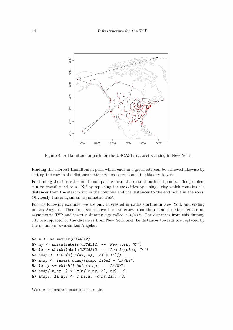
The found path is presented in Figure 4. It begins with New York and cities in New Jerseyand ends in a city in Manitoba, Canada.

Concorde and many advanced TSP solvers can only solve symmetric TSPs. To use thesesolvers, we can formulate the ATSP as a TSP using reformulate_ATSP_as_TSP() whichintroduces a dummy city for each city (see Section 2.2).

R> tsp <- reformulate_ATSP_as_TSP(atsp)

R> tsp


624 cities (distance ✬unknown✬)

After finding a tour for the TSP, the dummy cities are removed again giving the tour for theoriginal ATSP. Note that the tour needs to be reversed if the dummy cities appear before andnot after the original cities in the solution of the TSP. The following code is not executedhere, since it takes several minutes to execute and Concorde has to be installed separately.Concorde finds the optimal solution with a length of 36091.

R> tour <- solve_TSP(tsp, method = "concorde")

R> tour <- as.TOUR(tour[tour <= n_of_cities(atsp)])


160°W 140°W 120°W 100°W 80°W 60°W

20

°N3

0°N

40

°N5

0°N

60

°N7

0°N

80

°N

●

●

Figure 4: A Hamiltonian path for the USCA312 dataset starting in New York.

Finding the shortest Hamiltonian path which ends in a given city can be achieved likewise bysetting the row in the distance matrix which corresponds to this city to zero.

For finding the shortest Hamiltonian path we can also restrict both end points. This problemcan be transformed to a TSP by replacing the two cities by a single city which contains thedistances from the start point in the columns and the distances to the end point in the rows.Obviously this is again an asymmetric TSP.

For the following example, we are only interested in paths starting in New York and endingin Los Angeles. Therefore, we remove the two cities from the distance matrix, create anasymmetric TSP and insert a dummy city called "LA/NY". The distances from this dummycity are replaced by the distances from New York and the distances towards are replaced bythe distances towards Los Angeles.

R> m <- as.matrix(USCA312)

R> ny <- which(labels(USCA312) == "New York, NY")

R> la <- which(labels(USCA312) == "Los Angeles, CA")

R> atsp <- ATSP(m[-c(ny,la), -c(ny,la)])

R> atsp <- insert_dummy(atsp, label = "LA/NY")

R> la_ny <- which(labels(atsp) == "LA/NY")

R> atsp[la_ny, ] <- c(m[-c(ny,la), ny], 0)

R> atsp[, la_ny] <- c(m[la, -c(ny,la)], 0)

We use the nearest insertion heuristic.


R> tour <- solve_TSP(atsp, method ="nearest_insertion")

R> tour


result of method ✬nearest_insertion✬ for 311 cities

tour length: 45029

R> path_labels <- c("New York, NY",

+ labels(cut_tour(tour, la_ny)), "Los Angeles, CA")

R> path_ids <- match(path_labels, labels(USCA312))

R> head(path_labels)

[1] "New York, NY" "North Bay, ON" "Sudbury, ON"

[4] "Timmins, ON" "Sault Ste Marie, ON" "Thunder Bay, ON"

R> tail(path_labels)

[1] "Eureka, CA" "Reno, NV" "Carson City, NV"

[4] "Stockton, CA" "Santa Barbara, CA" "Los Angeles, CA"

R> plot_path(path_ids)

The path jumps from New York to cities in Ontario and it passes through cities in Californiaand Nevada before ending in Los Angeles. The path displayed in Figure 5 contains multiplecrossings which indicate that the solution is suboptimal. The optimal solution generated byreformulating the problem as a TSP and using Concorde has only a tour length of 38489.

4.3. Rearrangement clustering

Solving a TSP to obtain a clustering was suggested several times in the literature (see, e.g.,Lenstra 1974; Alpert and Kahng 1997; Johnson, Krishnan, Chhugani, Kumar, and Venkata-subramanian 2004). The idea is that objects in clusters are visited in consecutive order andfrom one cluster to the next larger “jumps” are necessary. Climer and Zhang (2006) callthis type of clustering rearrangement clustering and suggest to automatically find the clusterboundaries of k clusters by adding k dummy cities which have constant distance c to allother cities and are infinitely far from each other. In the optimal solution of the TSP, thedummy cities must separate the most distant cities and thus represent optimal boundariesfor k clusters.

For the following example, we use the well known iris data set. Since we know that the datasetcontains three classes denoted by the variable Species, we insert three dummy cities into theTSP for the iris data set and perform rearrangement clustering using the default method(nearest insertion algorithm). Note that this algorithm does not find the optimal solutionand it is not guaranteed that the dummy cities will present the best cluster boundaries.

R> data("iris")

R> tsp <- TSP(dist(iris[-5]), labels = iris[, "Species"])

R> tsp_dummy <- insert_dummy(tsp, n = 3, label = "boundary")

R> tour <- solve_TSP(tsp_dummy)


160°W 140°W 120°W 100°W 80°W 60°W

20

°N3

0°N

40

°N5

0°N

60

°N7

0°N

80

°N

●

●

Figure 5: A Hamiltonian path for the USCA312 dataset starting in New York and ending inLos Angles.

Next, we plot the TSP’s permuted distance matrix using shading to represent distances.The result is displayed as Figure 6. Lighter areas represent larger distances. The additionalred lines represent the positions of the dummy cities in the tour, which mark the clusterboundaries obtained.

R> ## plot the distance matrix

R> image(tsp_dummy, tour, xlab = "objects", ylab ="objects")

R> ## draw lines where the dummy cities are located

R> abline(h = which(labels(tour)=="boundary"), col = "red")

R> abline(v = which(labels(tour)=="boundary"), col = "red")

One pair of red horizontal and vertical lines exactly separates the darker from lighter areas.The second pair occurs inside the larger dark block. We can look at how well the partitioningobtained fits the structure in the data given by the species field in the data set. Since we usedthe species as the city labels in the TSP, the labels in the tour represent the partitioning withthe dummy cities named ‘boundary’ separating groups. The result can be summarized basedon the run length encoding of the obtained tour labels:

R> out <- rle(labels(tour))

R> data.frame(Species = out$values,

+ Lenghts = out$lengths,

+ Pos = cumsum(out$lengths))


20 40 60 80 100 120 140

20

40

60

80

10

01

20

14

0

objects

ob

jects

Figure 6: Result of rearrangement clustering using three dummy cities and the nearest inser-tion algorithm on the iris data set.

Species Lenghts Pos

1 boundary 1 1

2 setosa 50 51

3 boundary 1 52

4 virginica 1 53

5 versicolor 11 64

6 virginica 1 65

7 versicolor 36 101

8 virginica 8 109

9 versicolor 1 110

10 virginica 3 113

11 versicolor 1 114

12 virginica 6 120

13 versicolor 1 121

14 virginica 24 145

15 boundary 1 146

16 virginica 7 153

One boundary perfectly splits the iris data set into a group containing only examples of species‘Setosa’ and a second group containing examples for ‘Virginica’ and ‘Versicolor’. However, thesecond boundary only separates several examples of species ‘Virginica’ from other examplesof the same species. Even in the optimal tour found by Concorde, this problem occurs.The reason why the rearrangement clustering fails to split the data into three groups is thecloseness between the groups ‘Virginica’ and ‘Versicolor’. To inspect this problem further, we


●

●●

●

●

●

●

●

●

●

●

●

●

●

●

●

●

●

●

●

●●

●●

●

●

●

●●

●●

●

●

●

●

●

●

●

●

●●

●

●

●

●

●

●

●

●

●

−3 −2 −1 0 1 2 3 4

−1

.0−

0.5

0.0

0.5

1.0

PC1

PC

2

Figure 7: The 3 path segments representing a rearrangement clustering of the iris data set.The data points are projected on the set’s first two principal components. The three speciesare represented by different markers and colors.

can project the data points on the first two principal components of the data set and add thepath segments which resulted from solving the TSP.

R> prc <- prcomp(iris[1:4])

R> plot(prc$x, pch = as.numeric(iris[,5]), col = as.numeric(iris[,5]))

R> indices <- c(tour, tour[1])

R> indices[indices > 150] <- NA

R> lines(prc$x[indices,])

The result in shown in Figure 7. The three species are identified by different markers and allpoints connected by a single path represent a cluster found. Clearly, the two groups to the rightside of the plot are too close to be separated correctly by using just the distances betweenindividual points. This problem is similar to the chaining effect known from hierarchicalclustering using the single-linkage method.

5. Conclusion

In this paper we presented the R extension package TSP which implements an infrastructureto handle and solve TSPs. The package introduces classes for problem descriptions (TSP andATSP) and for the solution (TOUR). Together with a simple interface for solving TSPs, itallows for an easy and transparent usage of the package.


With the interface to Concorde, TSP also can use a state of the art implementation whichefficiently computes exact solutions using branch-and-cut.

Acknowledgments

The authors of this paper want to thank Roger Bivand for providing the code to correctlydraw tours and paths on a projected map.

References

Alpert CJ, Kahng AB (1997). “Splitting an Ordering into a Partititon to Minimize Diameter.”Journal of Classification, 14(1), 51–74.

Applegate D, Bixby R, Chvatal V, Cook W (2006). Concorde TSP Solver. URL http:

//www.tsp.gatech.edu/concorde/.

Applegate D, Bixby RE, Chvatal V, Cook W (2000). “TSP Cuts Which Do Not Conformto the Template Paradigm.” In M Junger, D Naddef (eds.), Computational CombinatorialOptimization, Optimal or Provably Near-Optimal Solutions, volume 2241 of Lecture NotesIn Computer Science, pp. 261–304. Springer-Verlag, London, UK.

Applegate D, Cook W, Rohe A (2003). “Chained Lin-Kernighan for Large Traveling SalesmanProblems.” INFORMS Journal on Computing, 15(1), 82–92.

Climer S, ZhangW (2006). “Rearrangement Clustering: Pitfalls, Remedies, and Applications.”Journal of Machine Learning Research, 7, 919–943.

Croes GA (1958). “A Method for Solving Traveling-Salesman Problems.”Operations Research,6(6), 791–812.

Dantzig G, Fulkerson D, Johnson S (1954). “Solution of a Large-scale Traveling SalesmanProblem.” Operations Research, 2, 393–410.

Garfinkel R (1985). “Motivation and Modeling.” In Lawler et al. (1985), chapter 2, pp. 17–36.

Gomory R (1963). “An algorithm for integer solutions to linear programs.” In R Graves,P Wolfe (eds.), Recent Advances in Mathematical Programming, pp. 269–302. McGraw-Hill, New York.

Gutin G, Punnen A (eds.) (2002). The Traveling Salesman Problem and Its Variations,volume 12 of Combinatorial Optimization. Kluwer, Dordrecht.

Hahsler M, Buchta C, Hornik K (2006). seriation: Infrastructure for seriation. R packageversion 0.1-1.

Hahsler M, Hornik K (2007). “TSP – Infrastructure for the Traveling Salesperson Problem.”Journal of Statistical Software, 23(2), 1–21. ISSN 1548-7660.

Held M, Karp R (1962). “A Dynamic Programming Approach to Sequencing Problems.”Journal of SIAM, 10, 196–210.

http://www.tsp.gatech.edu/concorde/

http://www.tsp.gatech.edu/concorde/


Hoffman A, Wolfe P (1985). “History.” In Lawler et al. (1985), chapter 1, pp. 1–16.

Hubert LJ, Baker FB (1978). “Applications of Combinatorial Programming to Data Analysis:The Traveling Salesman and Related Problems.” Psychometrika, 43(1), 81–91.

Johnson D, Krishnan S, Chhugani J, Kumar S, Venkatasubramanian S (2004). “CompressingLarge Boolean Matrices Using Reordering Techniques.” In Proceedings of the 30th VLDBConference, pp. 13–23.

Johnson D, McGeoch L (2002). “Experimental Analysis of Heuristics for the STSP.” In Gutinand Punnen (2002), chapter 9, pp. 369–444.

Johnson D, Papadimitriou C (1985a). “Computational complexity.” In Lawler et al. (1985),chapter 3, pp. 37–86.

Johnson D, Papadimitriou C (1985b). “Performance guarantees for heuristics.” In Lawleret al. (1985), chapter 5, pp. 145–180.

Johnson O, Liu J (2006). “A traveling salesman approach for predicting protein functions.”Source Code for Biology and Medicine, 1(3), 1–7.

Jonker R, Volgenant T (1983). “Transforming asymmetric into symmetric traveling salesmanproblems.” Operations Research Letters, 2, 161–163.

Land A, Doig A (1960). “An Automatic Method for Solving Discrete Programming Problems.”Econometrica, 28, 497–520.

Lawler EL, Lenstra JK, Rinnooy Kan AHG, Shmoys DB (eds.) (1985). The Traveling Sales-man Problem. Wiley, New York.

Lenstra J, Kan AR (1975). “Some simple applications of the travelling salesman problem.”Operational Research Quarterly, 26(4), 717–733.

Lenstra JK (1974). “Clustering a Data Array and the Traveling-Salesman Problem.” Opera-tions Research, 22(2), 413–414.

Lin S (1965). “Computer solutions of the traveling-salesman problem.”Bell System TechnologyJournal, 44, 2245–2269.

Lin S, Kernighan B (1973). “An effective heuristic algorithm for the traveling-salesman prob-lem.” Operations Research, 21(2), 498–516.

Padberg M, Rinaldi G (1990). “Facet identification for the symmetric traveling salesmanpolytope.” Mathematical Programming, 47(2), 219–257. ISSN 0025-5610.

Pebesma EJ, Bivand RS (2005). “Classes and methods for spatial data in R.” R News, 5(2),9–13. URL http://CRAN.R-project.org/doc/Rnews/.

Prim R (1957). “Shortest connection networks and some generalisations.” Bell System Tech-nical Journal, 36, 1389–1401.

Punnen A (2002). “The Traveling Salesman Problem: Applications, Formulations and Varia-tions.” In Gutin and Punnen (2002), chapter 1, pp. 1–28.

http://CRAN.R-project.org/doc/Rnews/


Ray SS, Bandyopadhyay S, Pal SK (2007). “Gene Ordering in Partitive Clustering usingMicroarray Expressions.” Journal of Biosciences, 32(5), 1019–1025.

Rego C, Glover F (2002). “Local Search and Metaheuristics.” In Gutin and Punnen (2002),chapter 8, pp. 309–368.

Reinelt G (2004). TSPLIB. Universitat Heidelberg, Institut fur Informatik, Im Neuen-heimer Feld 368,D-69120 Heidelberg, Germany. URL http://www.iwr.uni-heidelberg.

de/groups/comopt/software/TSPLIB95/.

Rosenkrantz DJ, Stearns RE, Philip M Lewis I (1977). “An Analysis of Several Heuristics forthe Traveling Salesman Problem.” SIAM Journal on Computing, 6(3), 563–581.

Affiliation:

Michael HahslerEngineering Management, Information, and SystemsLyle School of EngineeringSouthern Methodist UniversityP.O. Box 750123Dallas, TX 75275-0123E-mail: [email protected]

Kurt HornikDepartment of Finance, Accounting and StatisticsWirtschaftsuniversitat Wien1090 Wien, AustriaE-mail: [email protected]: http://statmath.wu.ac.at/~hornik/

http://www.iwr.uni-heidelberg.de/groups/comopt/software/TSPLIB95/

http://www.iwr.uni-heidelberg.de/groups/comopt/software/TSPLIB95/

mailto:[email protected]

mailto:[email protected]

http://statmath.wu.ac.at/~hornik/

tsp – infrastructure for the traveling salesperson problem

Documents