Extensions for

Forecasting Models1. Testing for trend (Daniel’s Test)

a. Daniel’s non-parametric testb. Testing when the error is normal

2. Forecasting Linear Trend:i. Linear regression,

ii. Holt’s, iii. Double moving average iv. Double Exponential Smoothing

3. Forecasting Curvilinear trendi. Simple exponential Growth

ii. Modifies Exponential Growthiii. Using Linear Regression to forecast

non-linear time series4. Seasonal time series5. Auto-Regressive time series

1

IntroductionIn this set of notes we discuss different types of time series, and the forecasting of their

future values. It is assumed that the student is familiar with forecasting models of

stationary time series such as moving average and exponential smoothing, of trended

time series such as the Holt’s model and linear regression, and of basic statistical

hypotheses testing and confidence intervals.

We look at time series with trend, seasonality, and autocorrelation component, for which

two types of forecasts are developed:

Single forecasts scheme – where the forecasting model is based on the whole set

of data available and all the data points have the same influence on the forecast

(e.g. linear regression).

The updating scheme – where the model’s parameters are changing with the

added information, and recent data influence the forecast more than older data

(e.g. exponential smoothing).

The general structure of these notes is as follows: First we test to detect a component of

interest (such as trend), then we present a single forecast model(s) and updating model(s).

We use examples to demonstrate the concepts, and Excel to solve them.

2

1. Testing the Presence of a Trend

A time series can exhibit non-stationary behavior in various ways. For example it may develop temporary “drift” which creates a cycle, or it may be trended, or seasonal. In this note we focus on the trend, which can be caused by demand changes due to population growth, improving technology that improves productivity, changes in social behavior (divorce rates, TV time), etc. Identifying the presence of trend will prevent the erroneous use of stationary models. Recall that a stationary time series can be formulated by Yt=0 + t , while a time series with trend is formulated by Yt = t + t where Tt is the trend component (for example, for linear trend Tt = 0 +1t). Stationary forecasting models produce horizontal forecasts of the formF t+ k= β0 for all k≥ 1; this means that the forecast for any period in the future remains the same: the current estimate of 0. Thus a stationary model dose not account for time effects. To demonstrate the possible “damage” of using a stationary model to produce forecasts for a trended time series assume an m-period moving average was used to forecast a linear trend time series. Let MAt(m) represent the moving average value as of time ‘t’. The average age of information used in calculating the moving average is: Average Age = [0+1+2+…+(m-1)]/m = (m-1)/2. Then, t-(m-1)/2 can be interpreted as the point in time where the moving average is centered, and a forecast for period t+p as of period‘t’ for the trended time series should be MAt(m)+1[(m-1)/2+p]. This demonstrates the possible error if using only MAt(m) to forecast a trended time series.

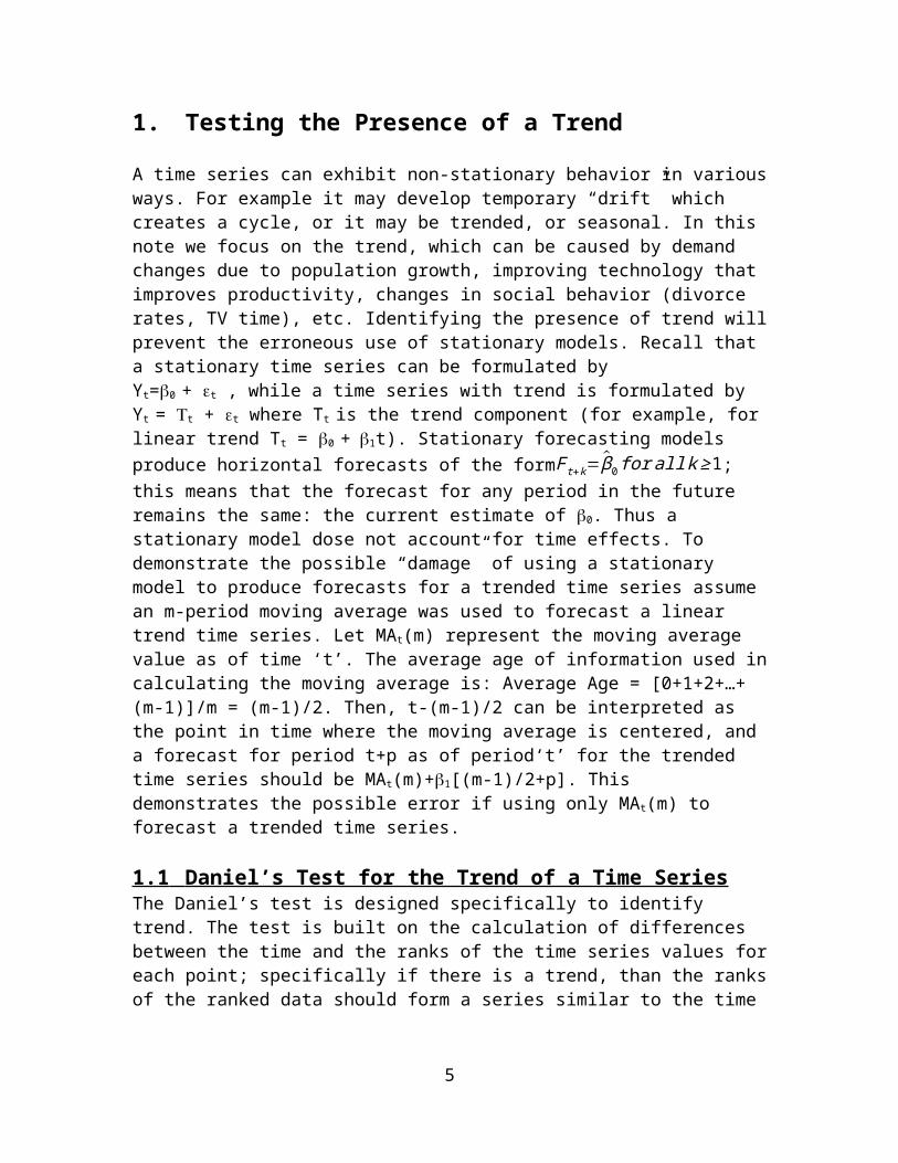
1.1 Daniel’s Test for the Trend of a Time Series The Daniel’s test is designed specifically to identify trend. The test is built on the calculation of differences between the time and the ranks of the time series values for each point; specifically if there is a trend, than the ranks of the ranked data should form a series similar to the time periods themselves. The following graph demonstrates the situation in a “perfect world”:

For the case shown above the difference between ‘t’ and the rank Rt assigned to Yt (that is (t – Rt)) is always zero. Since the time series is random, its behavior is not ‘perfect’ and

3

*

**

*

Time

Time Series

1 2 3 4

Y4

Y3

Y2

Y1

Ranks4

3

2

1

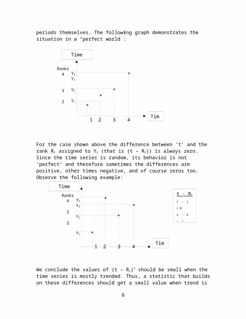
therefore sometimes the differences are positive, other times negative, and of course zeros too. Observe the following example:

We conclude the values of (t – Rt)2 should be small when the time series is mostly trended. Thus, a statistic that builds on these differences should get a small value when trend is present. More specifically, the statistic is a coefficient called The Spearman’s Correlation Coefficient calculated by rs = 1- [a function of‘t – Rt’). Because of the way the statistic is calculated the null hypothesis is rejected if rs is sufficiently large. More formally,

H0: = 0 (There is no trend)H1: 0 (There is trend)

Two cases need to be considered.

Case 1: n 30

The testing procedure depends on the existence or non-existence of ties in the time series.

No ties exist in the time series:

Sort the data from smallest to largest and rank them from 1 through n. Sort the ranks of Yt by the time t when Yt took place. Calculate the Spearman’s coefficient for the ranks:

(1 ) rs=1−6∑ d t

2

n(n2−1)Definitions:Rt = the rank of the data point that belongs to time period t. dt = t - Rt

n = the sample size (how many data points were recorded).

4

*

*

*

*

Time

Time Series

1 2 3 4

Y2

Y4

Y3

Y1

Ranks4

3

2

1

t - Rt

1 – 1 = 0

2 – 4 = -2

3 – 2 = +1

4 – 3 = +1

Reject the null hypothesis if |rs|> rcr, where the statistic rcr is a value taken from the Spearman table provided below (it depends on ‘n’ and

There are ties in the time series.After ranking the time series from smallest to largest and assigning ranks, average the ranks of each tie separately and assign the averaged rank of each tie to all the tie members. To calculate the correlation coefficient estimate, use the Pearson’s correlation definition for the ranks.

Pearson’s correlation coefficient:

r=Cov (t , Rt)

σ t σ R

We’ll use Excel to determine r, then test whether = 0. If this hypothesis is rejected then trend is present. To test we use the Fisher’s transformation.

(2 ) F (r )=.5 ln 1+r1−r

F(r) is approximately normally distributed with a = .5Ln[(1+)/(1-)] and

= 1/√n−3. So Z=.5 ln 1+r

1−r−.5 ln 1+ρ

1−ρ1

√n−3

is normally distributed and the Z statistic

becomes:

(3 ) Z=.5 ln 1+r

1−r1

√n−3

=(.5 ln 1+r1−r )√n−3.

H0 is rejected if |Z| > Z/2 The following two examples demonstrates the procedures when n < 30. The large sample case is discussed later.

Example 1(a)Test whether or not the following time series of sales exhibits any trend.

Time t Sales Sorted SalesTime of

Sorted Sales Ranks Dt2

1 9 5 11 1 1002 6 5.5 13 2 1213 13 6 2 3 14 11 7 5 4 15 7 7.5 7 5 46 8 8 6 6 07 7.5 9 1 7 368 10 10 8 8 09 14 11 4 9 25

10 11.5 11.5 10 10 011 5 12 12 11 1

5

12 12 13 3 12 8113 5.5 14 9 13 16

No ties were observed. We use Spearman’s coefficient: r s=1−6(100+121+…+16)13(132−1)

=¿

-.06

The critical value from Spearman’s table is r(n=13,.05) = .5549. There is insufficient evidence to support the presence of trend at 5% significance level.

Spearman critical values

One-Tailed : .001 .005 .010 .025 .050 .100Two-Tailed : .002 .010 .020 .050 .100 .200 n

6

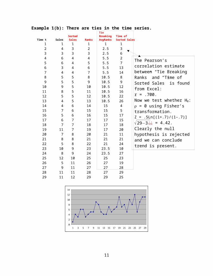
Example 1(b): There are ties in the time series.

Time t SalesSorted Sales

Ranks

Tie Breaking AvgRanks

Time of Sorted Sales

1 1 1 1 1 1

2 4 3 2 2.5

3

3 3 3 3 2.5 6

4 6 4 4 5.5 25 6 4 5 5.5 7

7

The Pearson’s correlation estimate between “Tie Breaking Ranks” and “Time of Sorted Sales” is found from Excel: r = .700.Now we test whether H0: = 0 using Fisher’s transformation.Z = .5Ln[(1+.7)/(1-.7)] √29−3¿¿ = 4.42. Clearly the null hypothesis is rejected and we can conclude trend is present.

6 3 4 6 5.5 137 4 4 7 5.5 148 5 5 8 10.5 89 5 5 9 10.5 9

10 9 5 10 10.5 1211 8 5 11 10.5 1612 5 5 12 10.5 2213 4 5 13 10.5 2614 4 6 14 15 415 7 6 15 15 516 5 6 16 15 1717 6 7 17 17 1518 7 7 18 17 1819 11 7 19 17 2020 7 8 20 21 1121 8 8 21 21 2122 5 8 22 21 2423 10 9 23 23.5 1024 8 9 24 23.5 2725 12 10 25 25 2326 5 11 26 27 1927 9 11 27 27 2828 11 11 28 27 2929 11 12 29 29 25

0

2

4

6

8

10

12

14

1 3 5 7 9 11 13 15 17 19 21 23 25 27 29

8

Case 2: n > 30In cases where the number of observations is greater than 30, rs is approximately normally distributed. When no ties occur the test statistic is calculated as follows:

(5 a ) Z=rs√n−1

H0 is rejected if |z| > z/2.

With ties we determine r as before by Excel, and run a t-test where

(5 b ) t= r

√ 1−rn−2

.

H0 is rejected if |t| > t/2,n-2.

1.2 Testing for trend when t is normal and independentNo assumption with respect to was necessary when applying Daniel’s test to the data. But when there is justification to believe the error term form a set of independent random variables normally distributed with a mean of “zero” and some standard deviation more powerful tests can be utilized for testing the presence of a trend. Under this assumption linear regression becomes a very attractive tool to help determine if there is trend present.

Testing linear relationship – the linear regression approachA ‘t – test’ is utilized when testing the validity of a linear regression model, that is when testing the existence of linear relationship between the time variable ‘t’ and the time series Yt. Recall: The linear regression is a model fitting procedure that determines the “best estimates” for the coefficients 0 and 1 of the linear trend model Yt = 0+1t+t. Once the estimated model Y t=b0+b1t was determined based on the data set available, a test is needed to verify linear relationship exists between the independent variable ‘t’ and the dependent variable Yt. Linear relationship exists when the slope ( 1) is not ‘zero’. So we test:H0: 1 = 0H1: 1 0

T statistic: t = b1−β1

Sβ1

=under H 0=b1

Sβ 1

.

Rejection rule: |t| > t/2,n-2 If H0 is rejected we have sufficient evidence at alpha% significant level to claim that linear relationship exists between‘t’ and Yt, which means that linear trend is present. Most of the time this test rejects H0 even when a non-linear trend is present!

9

Example 2: A large retailer is happy to experience an increase in sales over the last 16 quarters. Quarterly sales are shown:

Yt

177

187

211

237

220

255

300

351

401

360

520

575

545

558

560

580

t 1 2 3 4 5 6 7 8 9 10 11 12 13 14 15 16

Observing the graph that describes this time series we recognize an upward trend.

0 2 4 6 8 10 12 14 16 180

100

200

300

400

500

600

700

Yt

We want to statistically verify there is a linear trend present. We run regression analysis, and obtain the Excel output shown (assume the test for normality of the regression line errors (residuals) reveals the required normality):

SUMMARY OUTPUT

Regression StatisticsMultiple R 0.9652374R Square 0.9316833Adjusted R Square 0.9268035Standard Error 42.23754Observations 16

ANOVA

  df SS MS FSignificance

F

Regression 1 340617.3 340617.3190.9279

3 1.5E-09

Residual 14 24976.1371784.009

8Total 15 365593.44      

  CoefficientsStandard

Error t Stat P-value Lower 95%Upper 95%

Intercept 108.275 22.1495534.888360

60.000239

4 60.768934 155.78107

t 31.651471 2.290652213.81766

7 1.5E-09 26.73851 36.564431

Now we test whether the slope (trend) could be equal to zero.

10

H0: 1 = 0; H1: 1 ≠0. If the p-value < alpha, the null hypothesis (H0) is rejected in favor of H1, and we conclude that there is sufficient evidence (at alpha% significance level) that there is linear trend present in the time series. (This is just another approach to performing the t-test explained above). In this case, p-value = 1.5(10)-9, clearly less than any practical alpha value, so we conclude there is overwhelming evidence for linear trend. Moreover, since b1 = 31.65 > 0 the trend is positive.

Once the presence of trend was established a forecasting model needs to be fitted to the data.

2.1 Forecasting Linear Trend with Linear RegressionLinear regression with ‘time’ as the independent variable is a popular single forecast linear trend model. The model formulation is Yt = 0 + 1t + t. The parameters 0 and 1 are estimated by b0 and b1.

Forecasting p periods into the future

(6) Ft+p = b0 + b1(t+p), p = 1, 2, ...

Prediction interval

Recall that the error variable for the regression model is assumed to be normally distributed and independent. When and are all known the future value Yt+p is normally distributed with = (t+p)and = So the confidence interval for Y t+ pis Ft+p±Z/2However the more common case is when none of these parameters are known, thus need to be estimated from the sample. To

estimate we use the unbiased estimatorSε=√∑ (Y i−Y i)2

n−2. The prediction

interval is calculated for the regression as follows:

(7 ) F t+ p ± t α /2 , n−2 Sε √1+ 1n+

(t+ p−t )2

(n−1 )Var (t)

2.2 Forecasting Linear Trend with the Holt’s method The Holt’s method is an updating scheme, which can be considered an extension of the simple exponential smoothing model. It is adding a slope component to the intercept estimate (of the stationary model) since it is assuming the presence of linear trend. Thus in each step two estimates are made: (i) T(t) the trend estimate as of time t: T(t)=b0+b1t. (ii) b1(t) estimates the slope at time ‘t’.

Details are left for the student’s review.

Forecasting p periods into the future:

11

(8) Ft+p = Tt + b1(t)∙(t+p)

Prediction interval (9a) Ft+1 ±Z/2S

(9b ) F t+p± Z∝/2 Sε√1+α2 [(1+γ)2+(1+2 γ )2+…+(1+( p−1)γ )2 ] For p = 2, 3, …

2.3 Forecasting Linear Trend with Double Moving AverageThis method is based on the central location of the average.Notation MA(t,k) denotes the k-period moving average as of time t for the original

time series. MA'(t,k) denotes the k-period moving average as of time t for the series of

moving averages. T(t) denotes the slope of the time series as of period t.

In order to build a forecast for period t+p as of time‘t’, we need to estimate the slope and the series level as of time t. This is done next.

The estimated slope of the trended model as of time tMA(t,k) is centered (k-1)/2 periods behind t, at t-(k-1)/2. Explanation: A ‘k-period’ moving average contains the periods t, t-1, …, t-k+1. The center of this sequence is (t + t-k+1)/2 = t-(k-1)/2 MA'(t,k) is centered (k-1) periods behind t, at t-(k-1).Explanation: The information included in the k-period moving average of the k-period moving averages belong to periods t, t-1, … , t-2(k-1), centered at t-(k-1).

On an average basis and assuming a linear trend MA(t,k) - MA'(t,k) = [(k-1)/2]b1(t). This is so because the average is changing by T(t) units per period. Therefore,

(10 ) b1 , t=2

k−1 [M A t (k )−M A't(k )]

The estimated level of the trended model as of time t (T(t) = b0+b1t)L(t) is the expected value of the time series as of time t. So, on an average basis, the value of MA(t,k) is [(k-1)/2]b1(t) units different from T(t). Thus, T(t) = MA(t,k) + [(k-1)/2]b1(t) = MA(t,k)+[MA(t,k)-MA'(t,k)]. This leads to -

(11) 2 M At ( k )−MA 't (k )

With these two coefficient estimates we can now build a forecast as follows:

(12) Ft+p = T(t) + b1(t)∙p

The following example demonstrates the implementation of this model.

12

Example 3: Find the forecast for periods 14 and 15 of the following time series:

Calculating the model coefficients:

b1(13) = 2/(k-1)[MA(13,6) – MA’(13,6)] = 2/(6-1)[628.1667 – 598.08] = 12.03468

T(13) = 2MA(13,6) – MA’(13,6) = 2(628.1667) – 598.08 = 658.2534

Forecasting the time series for t +1= 14 and t +2= 15: (Note that currently t = 13).

F(14) = F(13+1) = T(13) + 1b1(13) = 658.2534 + 12.03468

F(15) = F(13+2) = T(13) +2 b1(13) = 658.25 + 2(12.03468)

2.4 Double Exponential SmoothingOne problem with the double moving average (DMA) model is the 2k-1 forecasts lost. Double Exponential Smoothing (DES) overcomes this problem. Much the same way as we did with the DMA model here too we’ll formulate the level and the slope estimates as follows:Define ES(t) as the smoothed value of the time series as of time t, and ES’(t) as the smoothed value of ES(t) as of time t. Specifically,

13

MA’(13,6)

1 5322 5463 5574 559

5 5546 5737 5748 604

9 61110 626

11 63612 64913 643

570.1667579.1667590.3333604.0616.6667628.1667

598.08

MA(13,6)

ESt = α Yt + (1 – α )ESt-1;

ES’t = α ESt + (1-α)ES’t-1.

The expected time series value at time t is:

T(t) = 2ESt – ES’t

The estimated slope as of time t is:

b1(t) = α

1−α (ESt – ES’t)

3. Forecasting Curvilinear Time SeriesCurvilinear time series are trended in a non-linear fashion. The rate at which the time series changes from period to period can be the same, can increase or decrease in a linear fashion, or can change over time. In what follows we observe two non-linear time series. The first one is quadratic where we apply the Holt’s updating approach to update the coefficients that generate the quadratic behavior and the second one is changing exponentially over time where a single forecast approach is implemented. Additional such models are listed at the end of this section without details.

3.1 Quadratic Trend – an Updating SchemeIn this section we present a modified Holt’s model, designed to forecast quadratic trend time series in an updating fashion. To do this we’ll need to estimate the trend component of the model as well as the quadratic function coefficients. Note that Yt = Tt + t, where Tt = 0+1t+2t2. First we exponentially smooth the time series three times:

A1 = A’1 = A”1 = Y1 (13a) At = Yt + (1– )At-1 t = 2, 3,…(13b) A’t = At + (1– )A’t-1

(13c) A”t = A’t + (1 –A”t-1)

Secondly we compute the trend estimate and the coefficient estimates as of time ‘t’ using the following relationships:

(14 a )T (t )=3 A t−3 A t'+At

' '

(14 b )b1 (t )= α2(1−α )2 [ (6−5 α ) At−(10−8 α ) At

'+ (4−3 α ) A t' ' ]

(14 c ) b2 (t )= α 2

(1−α )2(At−2 A t

'+A t' ' )

Finally the p period ahead forecast can be determined by:

14

Forecasting p periods ahead: Ft+p = T(t) + pb1(t)

(15 ) Ft+p=T t+p b1 (t )+12

p2b2(t )

Example 4There has been an impressive growth in the transportation sector of the economy from the 60th on. This was reflected by personal consumption expenditure. The following table summarizes this observation (in billions of dollars)

Year 1961 1962 1963 1964 1965 1966 1967 1968 1969 1970 1971 1972

Expenditure 44.8 47.4 49.5 54.3 58.4 60.4 63.3 69.3 75.5 80.6 92.3 105.4

Year 1973 1974 1975 1976 1977 1978 1979 1980 1981 1982 1983 1984

Expenditure 114.6 117.9 129.4 155.2 179.3 198.1 219.4 236.6 261.5 267.3 291.9 319.5

Draw the time series and fit a quadratic function to the data. We assume the time series is Yt = 0 + 1t + 2t2 + t.

1 2 3 4 5 6 7 8 9 10 11 12 13 14 15 16 17 18 19 20 21 22 23 240

50

100

150

200

250

300

350

Consumption

= .4 A1 = A’1 = A”1 = Y1 = 44.8A2 = Y2 + (1– )A1 = .4(44.8) + (1-.4)44.8 = 44.8A’2= A2 + (1– )A’1 = .4(44.8) + (1-.4)44.8 = 44.8A”2 = A’2 + (1 –A”1 = .4(44.8) + (1-.4)44.8 = 44.8T (2 )=3 A2−3 A2

' +A2' '=44.8

b1 (2 )= .42(1−.4 )2

[ (6−5(.4)) A2−(10−8(.4 )) A2' +(4−3(.4)) A2

' ' ] = 0

b2 (2 )= .42

(1−.4 )2(A2−2 A2

' +A2' ') = 0

A3 = .4Y3 + (1-.4)A2 = .4(57.2) + (1-.4)(44.8) = 50.904So on.At t=24 we have: T(24) = 317.8359; b1(24) = 22.9511; b2(24) = .7115

15

So

F24+1=T 24+1∙ b1 (24 )+ 12(1¿¿2)b2(24)¿ = 341.1428

F24+2=T 24+2 ∙b1 (24 )+ 12(22)b2(24) = 365.1612

F24+3=T 24+3 ∙ b1 (24 )+ 12(3¿¿2)b2(24)¿ = 389.8911

The alpha was optimized with Solver when minimizing MSE. * = .2873.

1 2 3 4 5 6 7 8 9 10 11 12 13 14 15 16 17 18 19 20 21 22 23 240

50

100

150

200

250

300

350

400

450

SeriesForecast

3.2 Simple Exponential growth model – a single forecast schemeThere are applications (economical, financial) where growth is exponential with a constant growth rate. The mathematical model that describes the behavior of such a time series is:

(11) Y t=β0 ∙ β1t ∙ εt

Typical examples are:

1 is the rate of change of this time series (note: in terms of average behavior, the trend ratio

t/1t-1 = 1, which represents the time series changes not including the errors).

A logarithmic transformation on both sides of the equation provides a linear model in ‘t’. Ln(Yt) = Ln(0)+ [Ln(1)]t+Ln(t), which can be re-written as Y’t = '0 + '1t + 't. We estimate the coefficients by using any selected procedure running on the transformed time series (such as linear regression), and obtain a logarithmic linear trend prediction equation.

16

0

0

To generate forecasts for the original time series we perform the anti-log transformation. See example next:

Example 5(a)A credit union is planning its investment strategy, and is trying to forecast the monthly loan requests for the next year. It collected loan request data over the last two years. Calculate the monthly forecast for next quarter on monthly basis using both the ratio and the logarithmic transformations.

The dataYear 1 297 249 310 305 307 381 449 465 485 500 550 580

Year 2 610 688 702 801 965 958 9771078

1165

1255

1248

1344

The time series graph is provided:

1 2 3 4 5 6 7 8 9 10 11 12 13 14 15 16 17 18 19 20 21 22 23 240

200

400

600

800

1000

1200

1400

1600

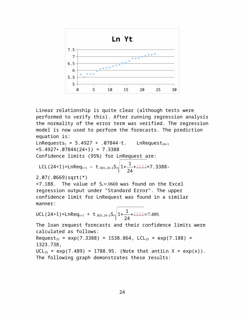
Logarithmic transformation: The transformed model is LnRequests = Ln0+Ln1∙t+ Lnt.

0 5 10 15 20 25 305

5.5

6

6.5

7

7.5

Ln Yt

Linear relationship is quite clear (although tests were performed to verify this). After running regression analysis the normality of the error term was verified. The regression model is now used to perform the forecasts. The prediction equation is:LnRequestst = 5.4927 + .07844∙t. LnRequest24+1 =5.4927+.07844(24+1) = 7.3388Confidence limits (95%) for LnRequest are:

LCL(24+1)=LnReqt+1 – t.025,24-2S√1+ 124

+¿¿¿¿=7.3388-2.07(.0669)sqrt(*)

17

=7.188. The value of Swas found on the Excel regression output under "Standard Error". The upper confidence limit for LnRequest was found in a similar manner:

UCL(24+1)=LnReqt+1 + t.025,24-2S√1+ 124

+¿¿¿¿

The loan request forecasts and their confidence limits were calculated as follows:Request25 = exp(7.3388) = 1538.864, LCL25 = exp(7.188) = 1323.738, UCL25 = exp(7.489) = 1788.95. (Note that antiLn X = exp(x)). The following graph demonstrates these results:

1 2 3 4 5 6 7 8 9 10 11 12 13 14 15 16 17 18 19 20 21 22 23 24 250

500

1000

1500

2000

2500

3000

Simple Exponential Growth – an Updating SchemeMuch the same way the logarithmic transformation was used above to produce forecasts based on the single forecast approach with linear regression, we can take advantage of the linearity of the transformed model, and apply (say) the Holt’s method to obtain Ft+p based on an updating scheme. Using the same example above, let us demonstrate a few steps of the Holt’s procedure: Example 5(b): Let = .9; = .5.T2 = Y’2 = LnY2 = Ln249 = 5.517b1(2) = Y’2 – Y’1 = Ln249 – Ln297 =5.517 – 5.693 = -.1763F3= T2 + b1(2) = 5.341T3 = .9Y’3 + (1-.9)F3 = 5.697b1(3) = .5(T3 – T2) + (1-.5) b1(3) = .00165F4= T3 + b1(3) = 5.698And so on. At t=24 we have: T24 = 7.2006; b1(24) = .0509; So F’24+1 = 7.2006+.0509 = 7.2515; F’24+2 = 7.2515 + 2(.0509) = 7.3024’ and the time series predicted values are: F24+1 = exp(7.2515) = 1410.22; F24+2 = exp(7.3024) = 1483.86.

Observe the graph:

18

1 2 3 4 5 6 7 8 9 10 11 12 13 14 15 16 17 18 19 20 21 220

200

400

600

800

1000

1200

1400

1600

1800

Series1Series2

Prediction interval can now be constructed using the prediction interval formula (7) provided above for the Holt’s model. Let us require 95% confidence level. S is estimated from the data as follows: Sε=√¿¿¿.

95% Prediction Interval for period 25= F ' 24+1 ±1.96 Sε

95% Prediction Interval for period 26= F ' 24+2 ±1.96 Sε √1+.92 ¿¿

The antilog procedure (exp(.)) will provide the confidence limits for the future forecast values of the time series F24+1, and F24+2.

There is some criticism on the simple exponential growth model regarding the unlimited growth it allows. A correction for this problem is suggested by the following model.

3.3 The Modified Exponential Growth Model The following model provides an asymptotic growth which can model the behavior if real processes over time.

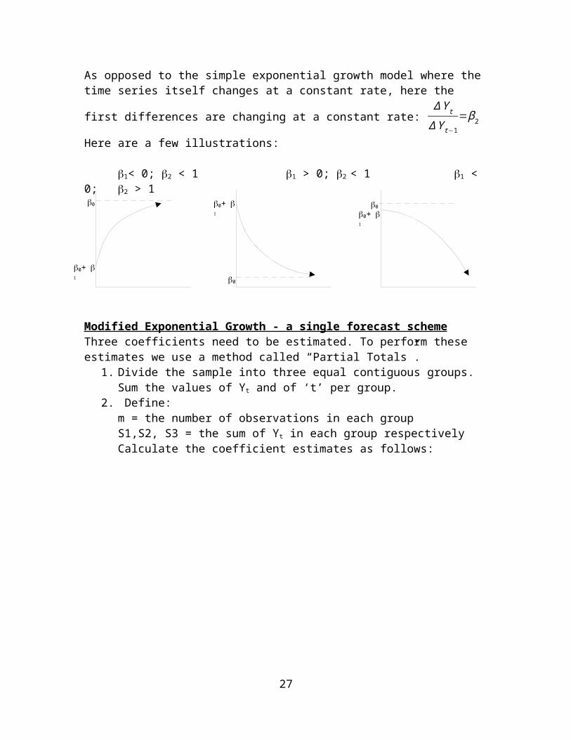
(16 ) Y t=β0+ β1 ∙ β2t ∙ εt

As opposed to the simple exponential growth model where the time series itself changes

at a constant rate, here the first differences are changing at a constant rate: ∆ Y t

∆ Y t−1=β2

Here are a few illustrations:

1< 0; 2 < 1 1 > 0; 2 < 1 1 < 0; 2 > 1

19

0

0

0

0+

0+

0+

Modified Exponential Growth - a single forecast schemeThree coefficients need to be estimated. To perform these estimates we use a method called “Partial Totals”.

1. Divide the sample into three equal contiguous groups. Sum the values of Yt and of ‘t’ per group.

2. Define:m = the number of observations in each groupS1,S2, S3 = the sum of Yt in each group respectivelyCalculate the coefficient estimates as follows:

20

(17 a ) (b2 )m=S 3−S2

S2−S1

(17b )b1=( S 2−S 1 ) ∙(b2−1)

[ (b2 )m−1 ]2b2

(17 c ) b0=1m (S 1−S2−S 1

(b2 )m−1 )

While the coefficients found with these formulae can be used to construct the prediction equation (see demonstration below) they can serve as an initial solution for optimization with Solver. We can then select a performance measure (usually MSE) and find the “best combination of b0, b1, and b2.

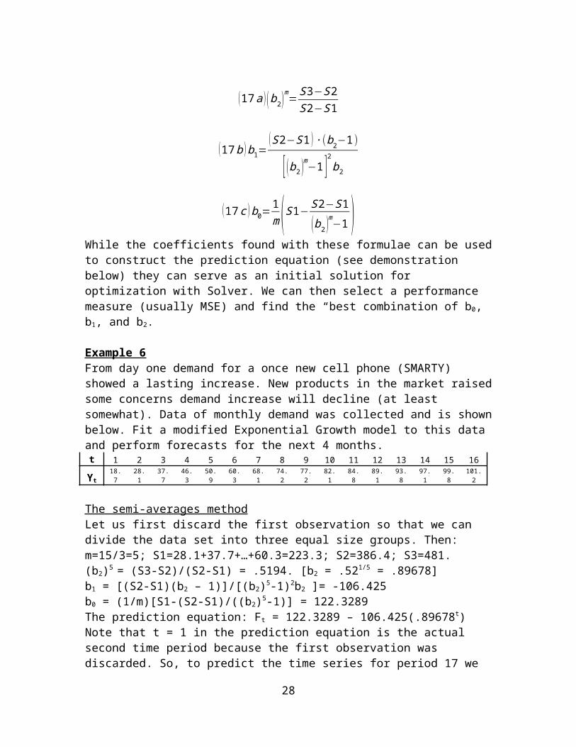
Example 6From day one demand for a once new cell phone (SMARTY) showed a lasting increase. New products in the market raised some concerns demand increase will decline (at least somewhat). Data of monthly demand was collected and is shown below. Fit a modified Exponential Growth model to this data and perform forecasts for the next 4 months.

t 1 2 3 4 5 6 7 8 9 10 11 12 13 14 15 16

Yt 18.7 28.1 37.7 46.3 50.9 60.3 68.1 74.2 77.2 82.1 84.8 89.1 93.8 97.1 99.8101.

2

The semi-averages method Let us first discard the first observation so that we can divide the data set into three equal size groups. Then: m=15/3=5; S1=28.1+37.7+…+60.3=223.3; S2=386.4; S3=481.(b2)5 = (S3-S2)/(S2-S1) = .5194. [b2 = .521/5 = .89678]b1 = [(S2-S1)(b2 – 1)]/[(b2)5-1)2b2 ]= -106.425b0 = (1/m)[S1-(S2-S1)/((b2)5-1)] = 122.3289The prediction equation: Ft = 122.3289 – 106.425(.89678t)Note that t = 1 in the prediction equation is the actual second time period because the first observation was discarded. So, to predict the time series for period 17 we substitute t = 16 in the equation: F16 = 122.3289 – 106.425(.8967816) =101.2481. Notice that the estimated asymptote (upper limit of the time series) is b0 = 113.49.

To improve this model we minimize MSE where b0, b1, and b2 are optimized, starting with the semi-averages approximated solution (122.3289, -106.425, .89678). The optimal solution found is b0 = 126.3964, b1 = -119.459, b2 = .9058. To predict the time series for period 17 we substitute t = 17(!) in the equation because no observation was dicarded: F17 = 126.3964– 119.459 (.905817).

The following plot describes the three time series involved:

21

1 2 3 4 5 6 7 8 9 10 11 12 13 14 15 160

20

40

60

80

100

120

YtSemiAvgsOptimal

The procedure shown above represents a single forecast approach. Updating schemes can smoothing approach.

Modified Exponential Growth - an updating schemeWe are using the Holt’s smoothing concept once again to produce required parameter estimates at each time t. The values estimated are Tt = 12

t, 2, and 0.

The recursive equations are:(18a) Tt = (Yt – b0,t-1) + (1 – ) Tt-1b2,t-1

(18b) b2,t = T t

T t−1 + (1 – )b2,t-1

(18c) b0,t = (Yt – Tt) + (1 – )b0,t-1

Forecasting k periods ahead is made by:

(19 ) Ft+k=b0 , t+T t (b2 , t )k

Initial valuesNoise (irregular movement) in the time series may cause serious problems in determining initial conditions as well as in fitting the model to the data. Thus it is recommended we first smooth the series without interfering with its exponential behavior, and then estimate the initial conditions using the following procedure. Dependent on the sample size, we can dedicate the first portion (say r observations) of the time series to obtain these estimates and start the updating process at period r + 1.

22

Use a p-period moving averages to smooth the time series for the first r periods. Let’s assume p is an odd number. The smoothed time series (denoted MA) should give an exponential growth profile with reduced noise. We use MAi to describe the ith moving average.

Determine b2,r = Avg(MA3- MA2)/(MA2- MA1); (MA4- MA3)/(MA3-MA2); ….(MAr-MAr-1)/(MAr-1-MAr-2)

Determine b1,r = Avg{(MA2 – MA1)/(b2,rp - b2,r

p-1); (MA3 – MA2)/(b2,rp+1 - b2,r

p); …}

Determine b0,r = Avg[MA1 – b1,r(b2 , r

p+12 ); M A2−(b2 ,r

p+32 ) ;…

If p is even, center the moving averages and use CMA instead of the MA.ExplanationsInitial value for b2: The average filtering constructs a time series which maintains the exponential behavior with reduced irregularities. Thus MA(t) ≅b0 + b1b2

t; [MA(t+1)-MA(t)]/[MA(t)-MA(t-1)] ≅ b2. Averaging these ratios leads to the initial value of b2.

Initial value for b1: MA(t)-MA(t-1) ≅ b1(b2t-b2

t-1) so [MA(t)-MA(t-1)]/[(b2t-b2

t-1)]≅b1

Initial value for b0: Results from MA(t) ≅b0 + b1b2t.

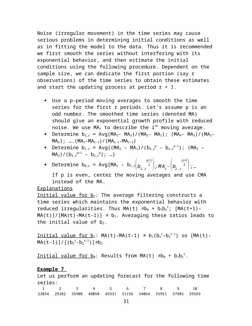
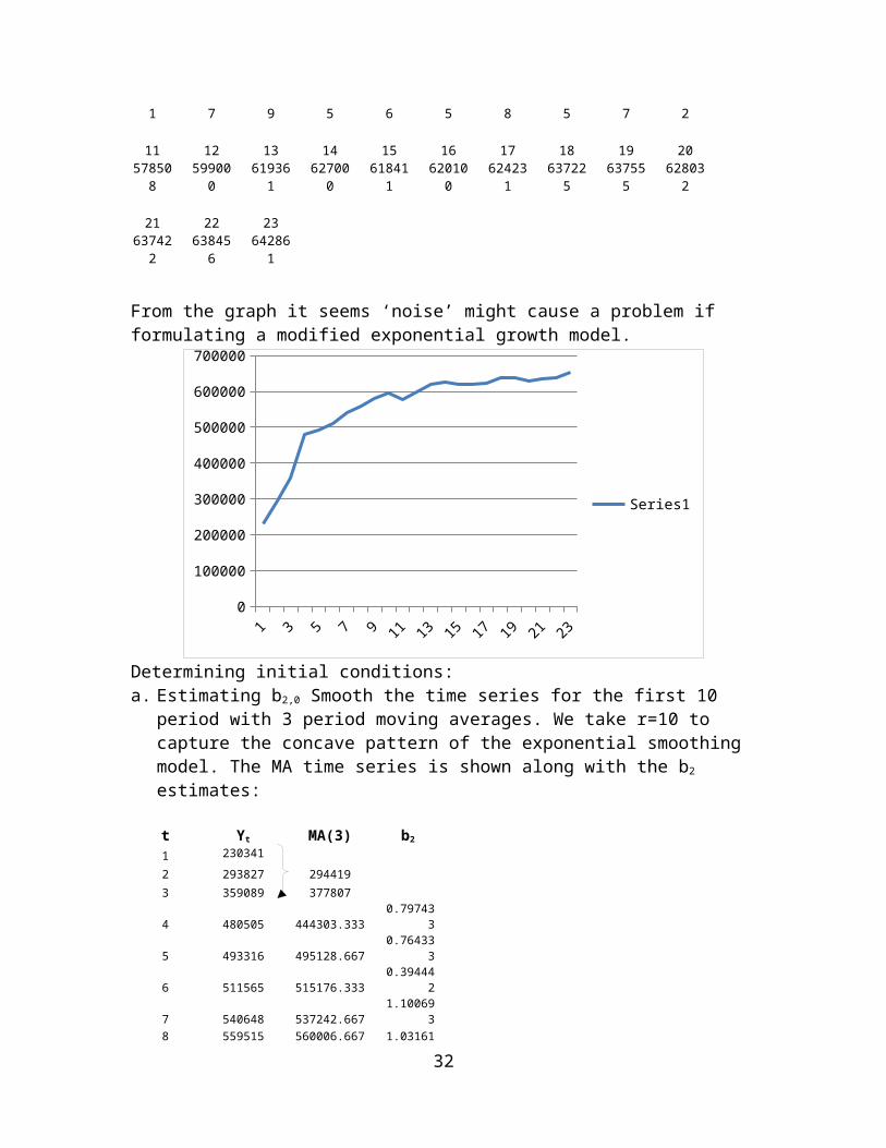
Example 7 Let us perform an updating forecast for the following time series:

1 2 3 4 5 6 7 8 9 10230341 293827 359089 480505 493316 511565 540648 559515 579857 595692

11 12 13 14 15 16 17 18 19 20578508 599000 619361 627000 618411 620100 624231 637225 637555 628032

21 22 23637422 638456 642861

From the graph it seems ‘noise’ might cause a problem if formulating a modified exponential growth model.

23

1 2 3 4 5 6 7 8 9 10 11 12 13 14 15 16 17 18 19 20 21 22 230

100000

200000

300000

400000

500000

600000

700000

Series1

Determining initial conditions:a. Estimating b2,0 Smooth the time series for the first 10 period with 3 period moving

averages. We take r=10 to capture the concave pattern of the exponential smoothing model. The MA time series is shown along with the b2 estimates:

t Yt MA(3) b2

1

230341

2 293827 2944193 359089 3778074 480505 444303.333 0.7974335 493316 495128.667 0.7643336 511565 515176.333 0.3944427 540648 537242.667 1.1006938 559515 560006.667 1.0316179 579857 578354.667 0.806009

10

595692

b. Estimating b1,0

t Yt MA(3) b2 b1

1

230341

2 293827 2944193 359089 377807 -6801244 480505 444303.333 0.797433 -6648485 493316 495128.667 0.764333 -6229396 511565 515176.333 0.394442 -301210

24

Avg = 0.815755

(377807 – 294419)/(.81573 - .81572)

(444303 – 377807)/(.81574 - .81573)

7 540648 537242.667 1.100693 -4064218 559515 560006.667 1.031617 -5139679 579857 578354.667 0.806009 -507827

10 595692

25

Avg = 0.815755 -528191

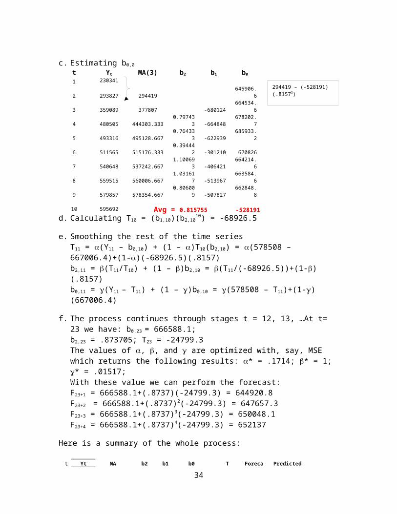
c. Estimating b0,0

t Yt MA(3) b2 b1 b0

1

230341

2 293827 294419 645906.63 359089 377807 -680124 664534.64 480505 444303.333 0.797433 -664848 678202.75 493316 495128.667 0.764333 -622939 685933.26 511565 515176.333 0.394442 -301210 6708267 540648 537242.667 1.100693 -406421 664214.68 559515 560006.667 1.031617 -513967 663584.69 579857 578354.667 0.806009 -507827 662848.8

10 595692

d. Calculating T10 = (b1,10)(b2,1010) = -68926.5

e. Smoothing the rest of the time series T11 = (Y11 – b0,10) + (1 – )T10(b2,10) = (578508 – 667006.4)+(1-)(-68926.5)(.8157)b2,11 = (T11/T10) + (1 – )b2,10 = (T11/(-68926.5))+(1-)(.8157)b0,11 = (Y11 – T11) + (1 – )b0,10 = (578508 – T11)+(1-)(667006.4)

f. The process continues through stages t = 12, 13, …At t= 23 we have: b0,23 = 666588.1;

b2,23 = .873705; T23 = -24799.3The values of , , and are optimized with, say, MSE which returns the following results: * = .1714; * = 1; * = .01517;With these value we can perform the forecast:F23+1 = 666588.1+(.8737)(-24799.3) = 644920.8F23+2 = 666588.1+(.8737)2(-24799.3) = 647657.3F23+3 = 666588.1+(.8737)3(-24799.3) = 650048.1F23+4 = 666588.1+(.8737)4(-24799.3) = 652137

Here is a summary of the whole process:

t Yt MA b2 b1 b0 T Forecast Predicted MA 

1 230341

2 293827 294419 645906.6 315518.8

3 359089 377807-

680124 664534.6 380278.8

4 480505 444303.333 0.797433-

664848 678202.7 433107

5 493316 495128.667 0.764333-

622939 685933.2 476201.9

6 511565 515176.333 0.394442-

301210 670826 511356.7

26

294419 – (-528191)(.81572)

(377807 – (-528191)(.81573)

Avg = 0.815755 -528191 667006.4

7 540648 537242.667 1.100693-

406421 664214.6 540034.5

8 559515 560006.667 1.031617-

513967 663584.6 563428.4

9 579857 578354.667 0.806009-

507827 662848.8 582512.210 595692 0.815755

-528191 667006.4

-68926.5 598079.9

11 578508 0.896004 666600.6

-61758.5 610779.3

12 599000 0.930043 666446.3

-57438.1 611670.5

13 619361 0.91114 666526

-52334.1 613586.5

14 627000 0.884423 666628.6

-46285.5 619322.6

15 618411 0.911388 666537 -42184 626070.516 620100 0.943857 666436.5

-39815.7 628560.4

17 624231 0.963768 666378.4 -38373 629426.118 637225 0.928796 666476.8

-35640.7 630023.7

19 637555 0.908688 666529.4

-32386.3 633903.4

20 628032 0.956682 666415.4

-30983.4 637577.3

21 636422 0.958629 666410.9

-29701.6 637365.1

22 638456 0.955641 666417.4

-28384.1 638533.6

23 652861 0.873705 666588.1

-24799.3 639881.4

24 644920.825 647657.326 650048.127 652137

Finally, some impressions:

Zooming at the smoothing and the forecasts:

27

1 2 3 4 5 6 7 8 9 10 11 12 13540000

560000

580000

600000

620000

640000

660000

YtForecast

28

The big picture:

1 2 3 4 5 6 7 8 9 10111213141516171819202122230

100000

200000

300000

400000

500000

600000

700000

YtForecastPredicted MA

29

The initial conditions lead to these predictions

Additional Transformations for a trended time series

The S- Shaped Trend - the Logistic Model Real applications exist where the time series shows a sharp increase at its initial steps, followed by declining growth and reaching a saturation level where there is virtually a flat behavior (a new product that matures). This situation can be modeled as follows:

(20 ) Y t=1

β0+β1∙ β2t

The general pattern is:

This curve is usually used for long term forecasting. The model requires reasonable amount of data beyond the infliction point, and data that “behave” in the sense that the estimated parameters yield an estimated model with fairly small errors. “Noisy” data will create markedly different forecasts produced in two consecutive periods for a period in the future. This analysis will not be further pursued.

Other transformationsYt = b0 + b1Ln t; Yt = b0eb1t; Yt = b0tb1

3.5 Using Linear Regression to Forecast time series

In what follows we’ll discuss four applications of linear regression in forecasting time series:

1. Transformations.2. Piece-wise linear time series3. Seasonal time series4. Autoregressive Models

Some of these topics stand alone, and others appear as part of other topics.

3.5.1 Transformations: When the time series Yt seems to be a non-linear function of ‘t’ it is sometimespossible to reformulate the series equation after the variables have been transformed.For example, if quadratic relationship between t and Yt are identified, reformulatingthe model by Y’t = b0+b1X1+b2X2 generates a linear model where X1 = t and x2 = t2,and linear regression analysis can be applied.

30

0

Example 8There has been an impressive growth in the transportation sector of the economy from the 60th on. This was reflected by personal consumption expenditure. The following table summarizes this observation (in billions of dollars)

Year 1961 1962 1963 1964 1965 1966 1967 1968 1969 1970 1971 1972

Expenditure 44.8 47.4 49.5 54.3 58.4 60.4 63.3 69.3 75.5 80.6 92.3 105.4

Year 1973 1974 1975 1976 1977 1978 1979 1980 1981 1982 1983 1984

Expenditure 114.6 117.9 129.4 155.2 179.3 198.1 219.4 236.6 261.5 267.3 291.9 319.5

Draw the time series and fit a quadratic function to the data. We assume the time series is Yt = 0 + 1t + 2t2 + t. The input is:

Expenditure t t2

44.8 1 247.4 2 449.5 . .54.3 . .

The prediction equation obtained is: Y t= 57.7131 – 2.5779t + .5764t2.The coefficient of determination is r2 = .997, which indicates almost a perfect fit to the data.Note that other transformations could be used, the modified exponential growth being one.

1 2 3 4 5 6 7 8 9 10 11 12 13 14 15 16 17 18 19 20 21 22 23 24 25 26 27 280

50

100

150

200

250

300

350

400

450

500

Y QuadraticConsumption

31

3.5.2 Piece-wise Linear time seriesReal applications exist where linear trend changes direction at a certain point(s) in time. This can be described by the following graph:

For example, sales may change in rate of increase when competition appears in the market. This modeling can also be useful when a non-linear trend is approximated by piecewise linear functions. The two equations shown in the graphical illustrations can be merged into one linear model by using a dummy variable as follows:Yt = b0 + b1t + b2(t – t0)I + t, where I = 0 if t t0 and I = 1 if t > t0. When I = 0 the equation is Yt = b0 + b1t + t, and when I = 1 the equation is Yt = (b0 – b2t0) + (b1 + b2)t + t. Then b0* = b0 – b2t0, and b1* = b1 + b2. To estimate the model coefficients we input Yt, t, and (t-t0)∙I as follows:

Yt t (t-t 0)I Y1 1 (1-t0)(0)Y2 2 (2-t0)(0)------------------------Yt0 t0 (t0-t0)(0)Yt0+1 t0+1 (1)(1)Yt0+2 t0+2 (2)(1)------------------------

To forecast p periods into the future we have

(21) Ft+p = (b0 – b2t0) + (b1 + b2)(t + p).

One might wonder why it is preferable to merge the two linear models into one model. The answer is that by extending the data set the error variance estimate becomes better (smaller) thus the t-tests and the prediction intervals more reliable.

32

t0

Yt(1) = b0 + b1t Yt

(2) = b0* + b1

* t

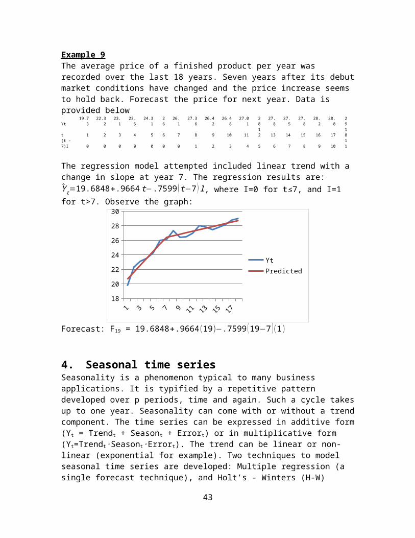
Example 9The average price of a finished product per year was recorded over the last 18 years. Seven years after its debut market conditions have changed and the price increase seems to hold back. Forecast the price for next year. Data is provided belowYt

19.73

22.32

23.1

23.5

24.31

26

26.1

27.36

26.42

26.48

27.01

28

27.8

27.5

27.8

28.2

28.8

29

t 1 2 3 4 5 6 7 8 9 10 1112 13 14 15 16 17

18

(t - 7)I 0 0 0 0 0 0 0 1 2 3 4 5 6 7 8 9 10

11

The regression model attempted included linear trend with a change in slope at year 7. The regression results are: Y t=19.6848+.9664 t−.7599 ( t−7 ) I , where I=0 for t≤7, and I=1 for t>7. Observe the graph:

1 2 3 4 5 6 7 8 9 10 11 12 13 14 15 16 17 1818

20

22

24

26

28

30

YtPredicted

Forecast: F19 = 19.6848+.9664 (19)−.7599 (19−7 )(1)

4. Seasonal time seriesSeasonality is a phenomenon typical to many business applications. It is typified by a repetitive pattern developed over p periods, time and again. Such a cycle takes up to one year. Seasonality can come with or without a trend component. The time series can be expressed in additive form (Yt = Trendt + Seasont + Errort) or in multiplicative form (Yt=Trendt∙Seasont∙Errort). The trend can be linear or non-linear (exponential for example). Two techniques to model seasonal time series are developed: Multiple regression (a single forecast technique), and Holt’s - Winters (H-W) technique (an updating scheme). Before presenting these models let us decide first whether or not the time series has seasonal movement. To test seasonality we need to isolate first the potential seasonal component from the time series (because trend might interfere with the testing procedure). Thus first we show how to “extract” the seasonality, then we discuss the tests to detect it.

33

4.1 The average filtering procedure to isolate seasonalityThis is a very popular method that does not require any assumption on the functional form of the trend.

Determine L period moving averages for all the time series available. That is calculate MA1 = (Y1+Y2+…+YL)/L; MA2 = (Y2+Y3…+YL+1)/L; etc.

If L is even calculate the centered moving average by averaging every two consecutive averages: CMA1 = (MA1+MA2)/2; CMA2 = (MA2+MA3)/2;…If L is odd the centering is not needed (then set CMA1 = MA1).

Calculate the seasonal ratio:

If Lis even :Y (L+2)/2

CMA 1,

Y ( L+ 4)/2

CMA 2…,∧if L is odd :

Y ( L+1 )/ 2

CMA 1,Y (L+3)/2

CMA 2…. These ratios

represent the time series cleaned of the trend, leaving us with seasonality (if exists) and irregularities only. Now we can perform the hypotheses tests for seasonality.

Example 10 For the following time series smooth out the seasonality, then test whether it is present. The data were collected quarterly (L=4).Solution:In the plot below you can clearly identify seasonality and possibly a trend.

1 2 3 4 5 6 7 8 9 10 11 12 13 14 15 16 17 18 19 200

20

40

60

80

100

120

140

160

180

200

Yt

The table summarizes the procedure:Yt t Season MA CMA Ratio

135.9

1 150.1

2 276.075

25.2 3 3 82.825 79.45 0.31718193.1 4 4 86.875 84.85 1.09723

162.9 5 1 87.675 87.275 1.86651466.3 6 2 96.425 92.05 0.72026128.4 7 3 94.525 95.475 0.29746

128.1 8 4 97.575 96.05 1.33368155.3 9 1 99.575 98.575 1.5754578.5 10 2 88.975 94.275 0.8326736.4 11 3 94.075 91.525 0.39770685.7 12 4 97.125 95.6 0.896444

175.7 13 1 100.625 98.875 1.77699190.7 14 2 107.725 104.175 0.8706550.4 15 3 108.4 108.0625 0.466397

34

25.2/79.45

114.1 16 4 108.975 108.6875 1.049799178.4 17 1 107.2 108.0875 1.650515

93 18 2 107.825 107.5125 0.86501643.3 19 3

116.6 20 4 The time series called “Ratio” should be “purely” seasonal. We test it next.

4.2 Kruskal-Wallis TestThis is a non-parametric test whose rationale is as follows: If no seasonality exists and the time series is purely random, then if we rank the observations a specific rank should be equally likely to fall in any season (that is there should not be a special concentration of, say, low ranks in any specific season). So the average rank in all seasons should be about the same. Define Ri = The sum of ranks of the Yt s in the ith cycle.ni = the number of specific seasonal in the ith cyclen = the total number of observations

Ri= R i

ni the average rank in the ith cycle

R=n+12 = the average rank

The statistic used to test the randomness is the weighted sum of squared differences between the average ranks within seasons and the overall average rank:

(22 ) H=∑ n i¿¿

The test procedure:H0: All Si = 0H1: At least one Si is not equal to zeroReject H0 if H >

2(L-1).

Example 11:Determine if the ratio time series from example 10 is indeed seasonal.The original St time series  St Sorted by Increasing orderSeries Season  Series Season Ranks

0.317181 3  0.29746 3 11.09723 4  0.317181 3 2

1.866514 1  0.397706 3 30.720261 2  0.466397 3 4

0.29746 3  0.720261 2 51.33368 4  0.83267 2 61.57545 1  0.865016 2 70.83267 2  0.87065 2 8

0.397706 3  0.896444 4 90.896444 4  1.049799 4 101.776991 1  1.09723 4 11

0.87065 2  1.33368 4 120.466397 3  1.57545 1 131.049799 4  1.650515 1 14

35

1.650515 1  1.776991 1 150.865016 2  1.866514 1 16

36

For example, R1 = 13+14+15+16 = 58 (see the ranks associated with quarter 1).

Another powerful approach relies on the assumption that the error term is normally distributed. We run the partial F-test to see whether the model with trend and seasonality is better than the model with trend only. In order to run this test we need to formulate a multiple regression with trend and dummy variables as explained below. This model will be used to detect the seasonality if present, and if so can then be used for forecasting.

4.3 Multiple Regression with Dummy variablesThe model discussed has an additive nature, where the trend effects are added to the seasonal effects. This formulation works well when the seasonal time series does not change its amplitude around the trend line over time. The time series with a cycle of L seasons can be formulated as follows:

(23) Yt = 0 + 1t + 2S1 + 3S2 + … + L+1SL + t.

The trend component (expressed by 0 + 1t is added to the seasonality expressed by 2S1 + 3S2 + … + LSL-1, where Si represents a dummy variable that gets the value 1 when the time series value belongs to season I, and zero otherwise. The beta coefficient 1 is the slope of the trend component. The beta coefficient associated with a seasonal dummy variable represents the seasonal average deviation of the time series from the trend level at that season.

Testing the presence of seasonality:In order to detect the presence of seasonality we need to compare two regression models:(i) The ‘trend only’ model. (ii) The trend + seasonality model. The question we try to answer is ‘whether or not adding a group of seasonal variables adds information to the trend model that was not there before’. To answer this question we test the coefficients of the dummy variables in the form of a partial F-test.

37

Season i 1 2 3 4

Ri 58 26 10 42Ri

2 3364 676 100 1764ni 4 4 4 4

Ri2/ni 841 169 25 441

H =14.1176

5

Chi-sq7.81472

8

p value 0.00274

9

2.05(4-1) = 7.8147, or

since the p-value is extremely small H0 is rejected, and we conclude seasonality is a factor.

H0: 2 = 3 = 4 = 0 (these are the coefficients of the dummy variables)H1: At least one is not zero

The test statistic:

(24 ) F=[ SSE (Trend )−SSE(Trend+Seasonal)

L−1 ]MSE (Trend+Seasonal)

The numerator reflects the improvement achieved when adding the seasonal variables and the denominator reflects the (still) unexplained variability of the complete model.

Rejection region: Reject H0 if F > F(L-1,n-L-1).If H0 is rejected we have sufficient evidence to conclude seasonality is present at % significance level.

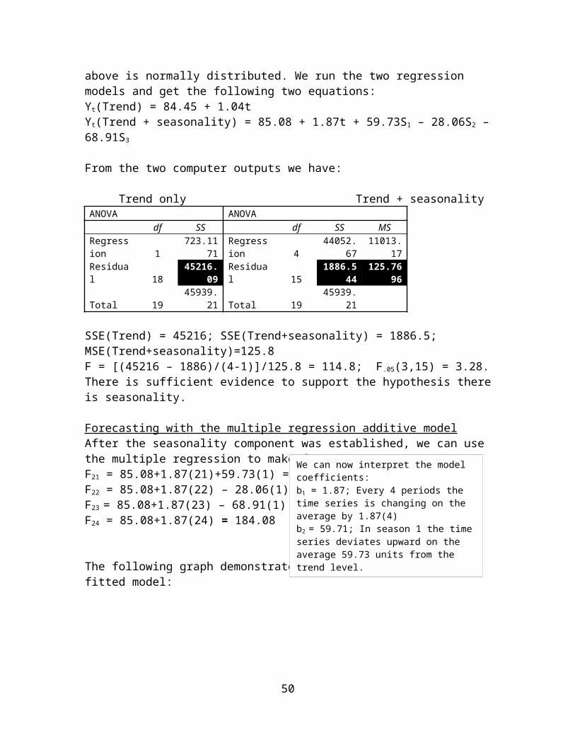
Example 11 continuedLet us assume now the error term of the multiple regression model with linear trend when run on the data of example 11 above is normally distributed. We run the two regression models and get the following two equations:Yt(Trend) = 84.45 + 1.04tYt(Trend + seasonality) = 85.08 + 1.87t + 59.73S1 – 28.06S2 – 68.91S3

From the two computer outputs we have:

Trend only Trend + seasonalityANOVA     ANOVA      

  df SS   df SS MSRegression 1

723.1171

Regression 4

44052.67

11013.17

Residual 1845216.0

9 Residual 151886.54

4125.769

6

Total 1945939.2

1 Total 1945939.2

1  

SSE(Trend) = 45216; SSE(Trend+seasonality) = 1886.5; MSE(Trend+seasonality)=125.8F = [(45216 – 1886)/(4-1)]/125.8 = 114.8; F.05(3,15) = 3.28. There is sufficient evidence to support the hypothesis there is seasonality.

Forecasting with the multiple regression additive modelAfter the seasonality component was established, we can use the multiple regression to make forecasts:F21 = 85.08+1.87(21)+59.73(1) = 129.96F22 = 85.08+1.87(22) – 28.06(1) = 59.18F23 = 85.08+1.87(23) – 68.91(1) = 98.16F24 = 85.08+1.87(24) = 184.08

38

We can now interpret the model coefficients:b1 = 1.87; Every 4 periods the time series is changing on the average by 1.87(4)b2 = 59.71; In season 1 the time series deviates upward on the average 59.73 units from the trend level.

The following graph demonstrates the time series and the fitted model:

39

1 2 3 4 5 6 7 8 9 10 11 12 13 14 15 16 17 18 19 200

20

40

60

80

100

120

140

160

180

200

YtForecast

4.4 Seasonal Time series with non linear trendA non-Linear trend with seasonality multiplicative model is introduced to demonstrate a curvilinear trend with time dependent seasonality. Note the regression based seasonal model introduced before allowed for a fixed seasonal effects over time only (represented by the beta coefficients of the dummy variables). This structure does not fit seasonal effects that (say) grow over time as the trend grows (in other words, the seasonal amplitude gradually increases over time). A seasonal extension of the simple exponential growth model where we use the technique of log transformation produces a multiple linear regression fitting procedure.The time series is modeled by

(25) Yt = (01t)(2

S13S2…L-2

S(L-1))t

The log transformation is:LogYt = Log0 + (Log1) t + (Log2)S1+ (Log3)S2+ …+ (LogL-2)SL-1+ Logt

The fitting process is based on the multiple regression as before, and when the prediction equation is obtained the forecast is computed by the antilog operation. Example 12Amazon sales have been growing steadily over the past 3 years. When observing the time series we detect an increasing rate at which the trend and the seasonal effects grow. The data and the time series plot are provided below,

Quarter Sales Quarter Sales Quarter Sales

1 573.889 1 1530.349 1 4135

2 577.876 2 1387.341 2 4063

3 637.858 3 1462.475 3 4264

40

4 972.36 4 2540.959

1 700.356 1 1901.6

2 667.625 2 1753

3 639.281 3 1858

4 1115.171 4 2977

1 847.422 1 2279

2 805.605 2 2139

3 851.299 3 2307

4 1428.61 4 3986

1 1083.559 1 3015

2 1099.912 2 2886

3 1134.456 3 3262

4 1945.772 4 5673

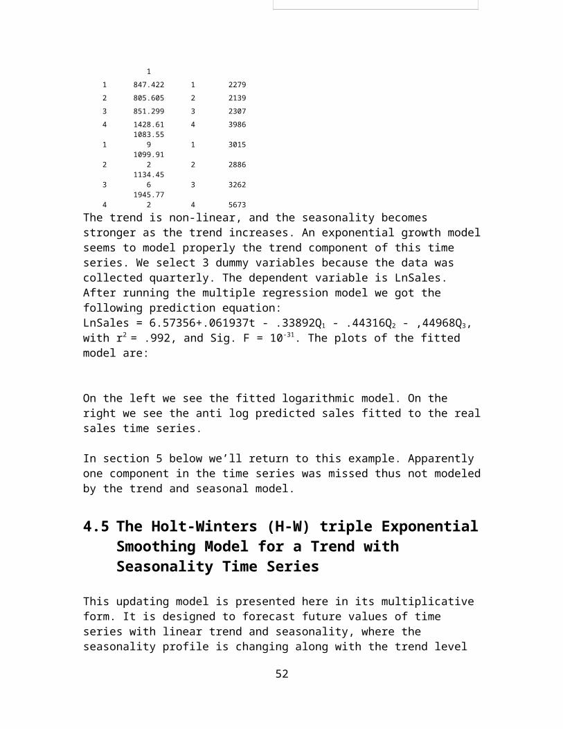
The trend is non-linear, and the seasonality becomes stronger as the trend increases. An exponential growth model seems to model properly the trend component of this time series. We select 3 dummy variables because the data was collected quarterly. The dependent variable is LnSales. After running the multiple regression model we got the following prediction equation:LnSales = 6.57356+.061937t - .33892Q1 - .44316Q2 - ,44968Q3, with r2 = .992, and Sig. F = 10-31. The plots of the fitted model are:

1 2 3 4 5 6 7 8 9 10 11 12 13 14 15 16 17 18 19 20 21 22 23 24 25 26 27 28 29 30 31 32 33 34 356

6.5

7

7.5

8

8.5

9

1 2 3 4 5 6 7 8 9 10 11 12 13 14 15 16 17 18 19 2021 22 23 24 25 26 27 28 29 30 31 32 33 34 350

1000

2000

3000

4000

5000

6000

On the left we see the fitted logarithmic model. On the right we see the anti log predicted sales fitted to the real sales time series.

41

1 2 3 4 5 6 7 8 9 10 11 12 13 14 15 16 17 18 19 20 21 22 23 24 25 26 27 28 29 30 31 32 33 34 350

1000

2000

3000

4000

5000

6000

Sales

In section 5 below we’ll return to this example. Apparently one component in the time series was missed thus not modeled by the trend and seasonal model.

4.5 The Holt-Winters (H-W) triple Exponential Smoothing Model for a Trend with Seasonality Time Series

This updating model is presented here in its multiplicative form. It is designed to forecast future values of time series with linear trend and seasonality, where the seasonality profile is changing along with the trend level over time. To describe the time series the trend component is multiplied by the seasonal index. As a result three parameters are to be estimated (smoothed). The first two deal with the linear trend, and the third one deals with the seasonal adjustment. Specifically, the time series to be forecasted can be formulated as follows:H-W with Linear Trend

(26) Yt = (0 + 1t)St+t

The linear part for this model (Tt = 0+1t) takes care of the trend effects, multiplied by St, a positive coefficient that represents the seasonality effect at each time‘t’. In case no seasonal adjustment is not needed at a certain period on top of the trend effects, then St=1. If the actual time series value falls above the trend line, then St>1; if the actual time series value falls below the trend line, then St<1. For example, if L(t0) = 10 at a certain t0, and if St0=.8, then Yt0 = 10(.8) = 8.

Let L represent the number of seasons per cycle. The H-W procedure uses the following three recursive formulas:

(27a) Tt = Yt/St-L + (1-)(Tt-1+b1,t-1)

(27b) b1(t) = (Tt – Tt-1) + (1 – )b1,t-1

(27c) St = Yt/Tt + (1 – )St-L

Explanation: The parameter Tt represents the linear trend of the time series at time’t’. The

smoothing approach to estimating Tt is utilized by that we weigh Yt/St-L against Tt-1. Yt/St-L (note that Yt/St-L = 0+1t) is the new estimate of the Tt; Tt-1 is the previous value of T that encompasses previous old information. These two estimates are combined using the smoothing coefficient .

The parameter b1,t represents the slope estimate of the trend line at time’t’. One estimate of this slope as of period t can be obtained by determining the change in the trend line between period t and period t-1: Tt – Tt-1 (note that 0+1t – (0+1(t-1)) = 1. This is considered new information because of the presence of Tt. The other estimate b1,t-1, is the trend estimate from the last period which encompasses information of all the previous periods. These two estimates are weighed against one another using the exponential smoothing approach with a smoothing coefficient .

42

The parameter St is the seasonal index pertaining to time’t’. One possible estimate of this index can be obtained by Yt/Tt (note that when dividing Y by the linear trend value we are left with the seasonal effect). A second estimate of the seasonal index is the last estimate made p periods earlier (St-L; recall that our cycle covers p periods). With these two estimates we can now apply the smoothing procedure using the coefficient .

The forecast for the time series k periods ahead is

(28) Ft+k = (Tt + kb1,t)St+k-L for k≤L

Comment: If k exceeds one cycle we need to pay attention to the seasonal cycles, because St+k-p yields yet uncalculated seasonal coefficients. Thus, a slight change in the formula is called for. Particularly, let k =mL+n (where m and n are integers greater than or equal to 1). Then we’ll use St-L+n instead of St+k-L. For example, if the forecast required is Ft+L+1 (i.e. k = L+1) we’ll use St-L+1; For Ft+L+2 we’ll use St-L+2; For Ft+2L that can be written as Ft+L+L use St-L+L = St; and for Ft+2L+1 we’ll use St-L+1 (same as for Ft+L+1, as should be). The example below demonstrates these concepts.

43

Initializing the Holt-Winters procedureInitiation of the H-W method depends on the amount of data available. In what follows we’ll proceed assuming at least two full cycles of data are available.

Obtaining initial valuesWe assume there are L seasons per cycle, and a time series of r observations is used for the estimation procedure. The method performs moving average filtering to smooth-out the seasonal effects first, then uses the de-seasoned time series that should consist of trend and random irregularities only to estimate the seasonal factors as well as the initial trend level. Let us look at example 13 in order to clarify the procedure.

Example 13:

Forecast the next 4 periods of this time series using the H-W triple exponential smoothing method with smoothing coefficients determined later by minimizing MAD.

  Year 1 Year 2 Year 3 Year 4 Year 5Q1 115.9 155.3 162.9 186.7 200.4Q2 30.1 78.5 66.3 100.7 123Q3 25.2 36.4 28.4 60.4 73.3Q4 73.1 85.7 128.1 124.1 146.6

Solution: Observing the data we notice that we have 5 years of data collected quarterly. So a cycle is considered one year and there are 4 seasons (L=4). We use the first 3 years to generate the initial values, and the last 2 years to optimize the model coefficients (alpha, beta, and gamma). This leads to: alpha = 0.04; beta = 0; gamma = 0.

Quarter

Time

Series MA CMA Ratio Adj S

Deseason

DeseasonFit T b1 S

Forecast

1 1115.

9 1.6968.5809

4 56.332

2 2 30.1 61.0750.911

333.0305

9 61.178

3 3 25.2 70.925 660.3818

20.389

864.6553

2 66.025

4 4 73.1 83.025 76.9750.9496

6 1.00972.4486

5 70.872

1 5155.

3 85.825 84.425 1.8395 1.6991.8949

1 75.719

2 6 78.5 88.975 87.40.8981

70.911

3 86.1429 80.566

3 7 36.4 90.875 89.9250.4047

80.389

893.3910

1 85.413

4 8 85.7 95.075 92.9750.9217

5 1.00984.9363

8 90.26

1 9162.

9 93.075 94.075 1.7316 1.6996.3920

2 95.107 1.69

2 10 95.3103.67

5 98.3750.9687

40.911

3104.578

6 99.9540.911

3

3 11 28.4109.62

5 106.650.2662

90.389

872.8655

2 104.80.389

8

4 12128.

1110.97

5 110.31.1613

8 1.009126.958

6 109.65109.6

54.8

5 1.009

1 13186.

7118.97

5114.97

51.6238

3 1.69110.475

1108.2

74.8

5 1.69 193.49

2 14100.

7117.97

5118.47

50.8499

70.911

3110.504

3 112.24.8

5 0.91 103.08

3 15 60.4 121.4119.68

80.5046

50.389

8154.967

5118.1

54.8

5 0.39 45.62

44

4 16124.

1126.97

5124.18

8 0.9993 1.009122.994

2115.7

84.8

5 1.01 124.1

1 17200.

4 130.2128.58

81.5584

7 1.69118.581

7114.0

54.8

5 1.69 203.85

2 18 123135.82

5133.01

30.9247

30.911

3134.975

5118.3

64.8

5 0.91 108.35

3 19 73.30.389

868.5809

4109.6

54.8

5 0.45 48.021

4 20146.

6 1.00933.0305

9108.2

74.8

5 1.15 129.21

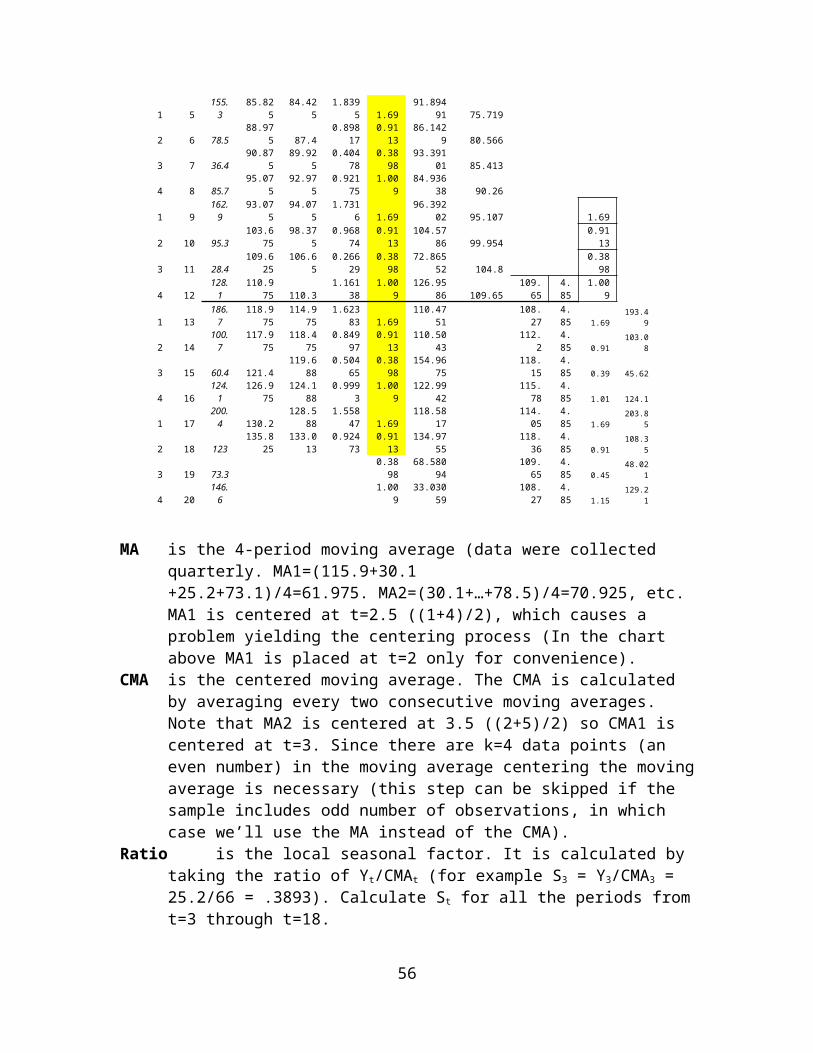
MA is the 4-period moving average (data were collected quarterly. MA1=(115.9+30.1 +25.2+73.1)/4=61.975. MA2=(30.1+…+78.5)/4=70.925, etc. MA1 is centered at t=2.5 ((1+4)/2), which causes a problem yielding the centering process (In the chart above MA1 is placed at t=2 only for convenience).

CMA is the centered moving average. The CMA is calculated by averaging every two consecutive moving averages. Note that MA2 is centered at 3.5 ((2+5)/2) so CMA1 is centered at t=3. Since there are k=4 data points (an even number) in the moving average centering the moving average is necessary (this step can be skipped if the sample includes odd number of observations, in which case we’ll use the MA instead of the CMA).

Ratio is the local seasonal factor. It is calculated by taking the ratio of Yt/CMAt (for example S3 = Y3/CMA3 = 25.2/66 = .3893). Calculate St for all the periods from t=3 through t=18.

AdjS is the seasonal factor estimate. To obtain it for a certain season: For each season average the ratios “Ratiot” that correspond to this season

(quarter). For example S(Quarter 1) = average(Ratio5, Ratio9, Ratio13, Ratio17)=average(1.8395,1.7316,1.6238,1.5585) =1.6884. This factor is assigned to all the time periods from t=1 through t = n that fall on quarter 1.

Normalize S of all the seasons. Normalizing means adjusting the seasonal factor S proportionately such that the sum of all seasonal factors in a cycle is L (L=4 here). This is done as follows:

AdjS(Season) =(L)(SSeason)/SSeason.

For example Adj S(Quarter 1) = 4(1.6884)/(1.8385+1.7316+1.6238+1.5585).

Deseason is the de-seasoned value of the time series at time t (Yt/AdjSt).DeseasonFit is the fitted de-seasonal trended model values at time t. In this problem we ran simple linear regression assuming the trend was linear. The line fits very well (r2 = .73), is very significant, and the error seem to be random. Now the initial values needed to initiate the H-W procedure can be obtained as follows (recall the H-W starts at period 13, the first quarter of year 4):Initial trend: T12 = Regression value at t=12: 108.99. See the table above. Initial slope: b1(12) = Regression slope = 4.7059.The H-W process can be started at t=13.

45

T13=(Y13/S13-4)+(1-)(T12+b1(12)) b1(13)=(T13-T12)+(1-)b1(12) S13=(Y13/T13)+(1-)S13-4

Forecast: F20+1=(T20+b1(20))S21-4; F20+2=(T20+2b1(20))S22-4

Comment on centering the averages:To understand this operation, note that the first average is centered at period (1+L)/2, the second average is centered at (3+L)/2 etc. If L is even, these centers fall between two periods. Therefore we produce a second set of averages, the centered average series that consists of the averages of all pairs as follows: CMA1=average(MA1,MA2); CMA2=average(MA2,MA3);…These averages are located at real time periods. For example, the first centered moving average (CMA1) is located at {(1+L)/2+[(3+L)/2}/2 =1+(1/2)L, which must be an integer since L is assumed to be even. This in turn means the center falls on a real time period. If L is odd, the centering operation is not needed. H-W with quadratic trend:The quadratic trend H-W procedure is similar to the linear trend H-W, but care should be given to the curvilinear trend component when smoothing the “quadratic change”. Let us define generally the time series as Yt = TtSt, and let Tt = 0 + 1t + 2t2 be the trend component; if Bi is the change in the trend value as of time i, then Bt can be determined by: Bt = Tt+1 – Tt = 1 + 2(2t+1). To perform H-W for this time series we need to smooth both Tt and Bt (as will become apparent shortly). While smoothing Tt is done in much the same way the linear trend case was handled, some attention should be given to the smoothing of B in the quadratic case. Smoothing B means weighing a new estimate of B as of t (Tt - Tt-1) and the previous estimate of B. However the rate at which T changes is not a constant, so we have to introduce the rate change of B into the smoothing scheme.

(28 a )T t=αY t

S t−L+ (1−α )(T t−1+B t−1)

(28 b ) Bt=β (T t−T t−1 )+ (1−β ) (B t−1+∆ Bt−1 ) (28 c ) ∆ B t = (Bt−B t−1 )+¿¿∆ Bt−1

(28 d ) S t=¿Y t

T t+¿)St-L

Obtaining initial values:We need to determine initial values for the trend (Tr), for the trend change (Br), for the change of B ∆ Br, and for the seasonal factors.

Determining Tr: After smoothing out the seasonality using the moving average filtering we are left with a quadratic trend of the form qt = 0 + 1t + 2t2 plus some irregularities. We fit a quadratic model to qt. From the quadratic fitting model we get the equation:

(28e) Qt = b0 + b1t + b2t2.

Let us assume r observations are used to fit the quadratic trend model, then Qr is the trend estimate as of time r, which in turn serves as the initial trend value for H-W. (Tr = Qr).

46

Determining Br and ∆Br. Based on our discussion above Br = b1,r+b2,r(2r+1). Since Bt = Bt-

1 + ∆Bt-1 we need to estimate the change ∆Bt-1. That is we need to find the ∆[∆ T t−1 ¿= 1

+ 2(2t+1) – [1 + 2(2t-1)] = 2Thus ∆Br = 2b2,r, where b1,r and b2,r are taken from the quadratic trend equation (28e) mentioned above. If linear regression was used then b1,r = b1 and b2,r = b2, and if some updating scheme was used (such as the quadratic Holt’s method) then we use the estimates of 1 and 2 as of time r.

Determining seasonal factors:The initials seasonal factors are determined the same way as before, from the moving average filtering.

Forecasting k periods into the future

(29) Ft+k = {Tt+kBt + (k-1)∆Bt}St+k-L for k≤L.

Example 14The following time series describes the monthly total number of passengers (in thousands) on US domestic flights. Let us apply the H-W quadratic model to this data set in order to forecast air-traffic in the next 12 months.

SolutionFirst let us look at the time series plot.

1 4 7 10 13 16 19 22 25 28 31 34 37 40 43 46 49 52 55 58 61 64 67 70 73 76 793000.00

3500.00

4000.00

4500.00

5000.00

5500.00

6000.00

Domestic Miles

It seems the trend is curvilinear. It also seems the seasonality effects are not changing over time. An additive model should provide proper forecasts, but this approach is not pursuit here (we’ll return to this problem in one of our assignments later). The Holt – Winters ApproachThere are 81 observations, which give us 6 full seasonal cycles of L=12 seasons each. We’ll use the first 4 years to estimate the initial conditions for H-W, and the last two years and 9 months for the optimization of the forecasting parameters. We start with the

47

12 period moving average filtering of the time series. The outcome of this operation is partially shown:

48

t Month Domestic Miles MA CMA Ratio Adjusted S Deseason t t-sqPredicted

Y

1 1 3299.96 0.89509 3686.74 1 1 3720.868

2 2 3259.21 0.86097 3785.51 2 4 3747.151

3 3 4142.83 1.05582 3923.82 3 9 3773.338

4 4 3847.95 1.00309 3836.09 4 16 3799.427

5 5 3991.16 1.02383 3898.25 5 25 3825.418

6 6 4290.213896.8

7 1.09403 3921.49 6 36 3851.313

7 7 4527.503916.8

33906.8

5 1.158862 1.15514 3919.45 7 49 3877.11

8 8 4542.053943.6

33930.2

3 1.15567 1.1186 4060.49 8 64 3902.81

9 9 3421.643956.6

33950.1

3 0.866208 0.89235 3834.4 9 81 3928.41210 10 3907.93

3959.56

3958.09 0.987327 0.98189 3980

10 100 3953.917

11 11 3635.12

3967.80

3963.68 0.917108 0.93809 3875.01

11 121 3979.325

12 12 4136.43

3976.92

3972.36 1.041302 0.98111 4216.08

12 144 4004.636

13 1 3621.50

3990.17

3983.54 0.909114 0.89509 4045.97

13 169 4029.849

14 2 3415.28

4015.56

4002.86 0.85321 0.86097 3966.79

14 196 4054.965

15 3 4177.89

4028.57

4022.06 1.038744 1.05582 3957.02

15 225 4079.984

16 4 3946.92

4050.27

4039.42 0.977102 1.00309 3934.76

16 256 4104.906

17 5 4100.52

4070.27

4060.27 1.009913 1.02383 4005.07

17 289 4129.73

18 6 4449.25

4095.12

4082.70 1.089782 1.09403 4066.86

18 324 4154.457

Below you can observe the de-seasoned time series. From the graph it seems the seasonality has indeed been cleared while the trend seems to be quadratic.

1 4 7 10 13 16 19 22 25 28 31 34 37 40 43 46 49 52 55 58 61 64 67 70 73 76 793000

3500

4000

4500

5000

5500

Deseason

49

After the seasonal effects were smoothed out the seasonal ratios were calculated for t = 7 through t=18 by Yt/CMAt, and the seasonal coefficients “S” computed by averaging all the ratios that belong to the same season. Then the “S” ratios were added to each season where missing (see the numbers in itelic bold). The ratios were then normalized (adjusted proportionately) such that their sum is 12, renamed “Adjusted S”, and the de-seasonal values were calculated by Yt/Adj St.

The de-seasonal time series was now fitted by a quadratic equation using linear multiple regression of the form qt = b0+b1t+b2t2+t. The model provided a very good fit to the data (r2 = .93) and was very significant (Sig F = 1.04(10)-26). The equation obtained from running the model over the time periods t=1 through t=48 (four years) was Qt = 3694.48+26.43t - .048t2. This equation provided the needed initial estimates as follows:Q48 = 3708.796+26.53(48) - .0488(48)2=4869.81 = T48

b1,48 = 26.53 b2,48 = -.0488

Performing H-W smoothing:T49=(Y49/S49-12)+(1-)[T48+B48] B49 = (T49-T48)+(1-)(B48+∆B48)∆B49 = (B49-B48) + (1-)∆B48

S49 = (Y49/L49)+(1-)S49-12

Alpha, beta, gamma, and delta were determined when minimizing MSE for the H-W model over periods 49 through 81: = .3148, = .5177 , = 1, = .16146.Continuing the smoothing by the same manner we approach t=82 with:

T81 B81 B81 S81

4616 -70.92 -15.6 0.898

Forecasts for future periods:

F82 = {T81+1B81}S82-12

F83 = {T81+2B81+∆B81}S83-12

F84 = {T81+3B81+2∆B81}S84-12

1 3 5 7 9 11 13 15 17 19 21 23 25 27 29 31 33 35 37 39 41 43 453000

3500

4000

4500

5000

5500

6000

50

B48 = 26.53+(-.0488)[2(48)+1] = 21.7964∆B48 = 2(-.0488) = -.0976

5.2. Autoregressive Forecasting ModelsIf a time series with trend, seasonality, or trend plus seasonality was properly modeled, we would expect the error variable to form a stationary/random time series. However, it is possible that in spite of properly identifying the presence of trend and seasonality, the error term will not form a random time series. This happens when the error terms are auto-correlated. Autocorrelation means relationships exist between pairs of the error variable located k periods apart. If the error terms are auto-correlated so do the time series values, a characteristic that needs to be taken care of by a proper modeling. Auto-regressive models are the answer. In what follows we look at two examples both with trend and seasonal components. The first example does not need any further alternative modeling (other than the original multiple regression based model) because auto-correlation analysis shows no such relationship exist. The second example will need further study of the errors to eliminate auto-correlation.

Example 15In order to compare performance of a specific company with the national industry as a whole, the Census Bureau tracks retail sales monthly. The data appear in the file Ex15 and the graph of these data reveals trend and seasonality. A multiple regression with trend and 11 dummy variables was run and provided a very good fit (r2 = .993), and significance (Sig. F = 0). When plotting the residuals vs. time we have no reason to suspect autocorrelation is present.

-10 10 30 50 70 90 110

-2000

-1500

-1000

-500

0

500

1000

1500

2000

Residuals

A graphical method that may support this observation is the lagged residual plot of et against et-1. If the pairs are concentrated in the first and third quadrant we probably have a positive one lag autocorrelation, and if they are concentrated in the second and forth, we probably have a negative one-lag auto-correlation. In this example the residuals are evenly spread in all the quadrants indicating no first order correlation.

51

-2000 -1500 -1000 -500 0 500 1000 1500 2000

-2500

-2000

-1500

-1000

-500

0

500

1000

1500

2000

We can support these observations by several statistical procedures. A non parametric test designed to detect autocorrelation (but may miss the presence of trend) is:

5.1 The Runs Test for randomness:Runs are defined as a sequence of errors on the same side of a certain predetermined level of reference. This level can be the error mean, or the error median etc. If the errors are positively auto-correlated then groups of consecutive errors reside close to one another – forming a small number of runs. If the errors are negatively auto-correlated then errors are changing sign frequently – forming a large number of runs. If the errors are not auto-correlated the number of runs will be moderate. This logic yields the following test. H0: The error time series is random (the number of runs is not extreme)H1: The error time series is not random (the number of runs is either very small or very large).

Let n be the sample size. Let m be the number of observations above (or below) the

median. Note: m=n−12 if n is odd, and m=n

2 if n is even. A random time series should

produce a random series of pluses and minuses (above and below the median respectively), thus not too many not too little number of runs. The number of runs R in a random sequence has the following mean and standard deviation:

(30 ) μR=m+1

(31 ) σ R=√ m(m−1)2 m−1

For m≤ 20 two critical values RU (upper critical) and RL (lower critical) can be obtained from a run test table (by Swed and Eisenhart, 1943), for a 5% significance level of a one tail test or a 10% two tail test. The table is shown in the next page. For m > 20, R is approximately normally distributed with a mean R and standard deviation R.

52

Residualt-1

Residualt

Example 15 - continuedIn the retail example above n = 103; m = (103-1)/2 = 51; R = m+1 = 51+1 = 52;

σ R=√ 52(51)2(52)−1

=5.07; R=59; Since m>20 we can use the normal distribution.

Z=59−525.07

=1.38. Since Z.025 = 1.96, there is insufficient evidence at 5% significance

level to claim the residuals arise from a non-random time series.

The Critical R for Runs Testm RL RU

1-4 - -5 2 10

6 3

11

7 3 138 4 149 5 15

10 6 1611 7 1712 7 1713 8 1914 9 2015 10 2216 11 2317 11 2518 12 2619 13 2720 14 28

The multiple regression with dummy variables seems to provide adequate forecasts. This will not be the situation in the next example.

In this example we are faced with a time series where trend was identified and modeled, only to realize that auto–correlation creates non-randomness within the error time series. Remedy is suggested.

Example 16

53

Reject H0 at 10% significance level for a two tail test, or 5% significance level for a one tail test if R≤ RL∨R ≥ RU.If H0 is rejected there is sufficient evidence in the sample to argue that the time series is auto-correlated.

For the last two years a department store has carried a new type of electronic calculator. Sales have generally increased, but demand seems to fluctuate randomly. To better understand the sales behavior over time and better plan inventories management is interested in developing a forecasting model.

54

Yt 238 245 263 247 239 234 245 240 242 248 261 294t 1 2 3 4 5 6 7 8 9 10 11 12Yt 288 310 335 368 356 393 363 386 426 422 358 384t 13 14 15 16 17 18 19 20 21 22 23 24

1 2 3 4 5 6 7 8 9 10 11 12 13 14 15 16 17 18 19 20 21 22 23 24200

250

300

350

400

450

Yt

Running Daniel’s test the presence of trend is verified. Both a linear trend model and a quadratic model are tried. Both models show a good fit (r2>.83), both are significant, but in both the auto correlation is a problem. For example for the quadratic model, there seems to be a clear first lag positive auto-correlation as observed in the lagged residual plot of et vs. et-1.

-60 -40 -20 0 20 40 60

-60

-40

-20

0

20

40

60

The Runs Test for the quadratic model confirms this observation. The errors form a non-random time series with positive first order auto-correlation.

An auto regressive model may solve this problem.

5.2 Forecasting with autoregressive modelsAutoregressive models use the possible autocorrelation between the time series values to predict values of the time series in future periods. In autoregressive models the time series is regressed on lagged value of the same time series. In other words, it is believed past values of the time series can explain current and future values. A first order (lag-1) autocorrelation refers to the magnitude of association between consecutive observations in the time series. The autoregressive model that expresses first order correlation is

(32a) Yt = B0 + B1Yt-1 + t.

55

A p-order autocorrelation refers to the size of correlation between values p periods apart. The autoregressive model that expresses a p-order time series is

(32b) Yt = B0 + B1Yt-1 + B2Yt-2 + … +BpYt-p + t.

The autoregressive forecasting model takes advantage of all the information within p periods apart from period t in order to build a forecast for period t+1. The coefficients B0,

Bt, Bt-1, …, Bt-p+1 are estimated using regression analysis. Note that the time series itself is used multiple times as “independent variables”. The following chart demonstrates the use of the time series to perform the regression analysis. Note how the data is organized.

In this chart the regression can be run from the fourth row down; therefore the first three rows of information are lost. This model tries to predict the value of Yt using Yt-1, Yt-2, and Yt-3 as explanatory variables (for example, Y5= e in the fourth row is explained by the values Y4=d, Y3=c, and Y2=b).

Determining the number of lagged variables.The problem of losing some information as demonstrated above when running an autoregressive model might become serious if the data set is not large while the order ‘p’ used is. One does not want to include too many periods in a model if they do not contribute significant information. There are several methods to discover the periods relevant to the autoregressive model. One method is recommended here.

IMPORTANT: Autoregressive models run on stationary time series only. When a time series is not stationary measures need to be taken in order to de-trend it. This will be discussed briefly later.

Example 16 – continuedReturning to the calculator sales example, we realize that an autoregressive model cannot be used without taking care of the trend that was found to be present in the time series. There are methods to de-trend time series and then perform the auto-regression. Another approach that seems to perform better is to include a time component in the auto-regressive equation that will account for the time dependence present.

Let us start with a lag-3 auto-regressive model (if it turns out that Yt-3 is significant, we extend the model to 4-lags, and if not we’ll reduce the model to 2-lags). The resulting model is:

56

Yt Yt-1 Yt-2 Yt-3

abcdef

abcde

abcd

abc

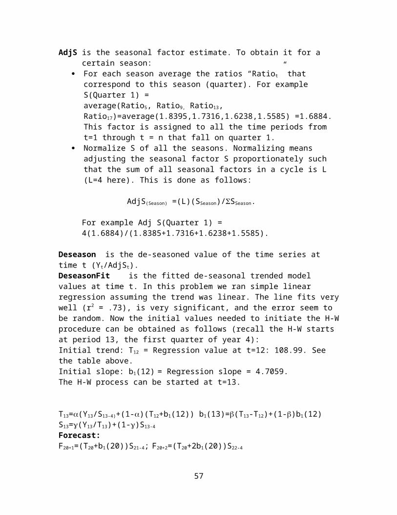
Yt = 0 + 1Yt-1 + 2Yt-2 + 3Yt-3 + 4t + t.

Here is an excerpt of the data set:Yt Y(t-1) Yt-2) Y(t-3) t238 1245 238 2263 245 238 3247 263 245 238 4

The output reveals the following results:

  CoefficientsStandard

Error t Stat P-valueIntercept 96.9966567 44.892799 2.160628 0.046236Y(t-1) 0.48837567 0.1524099 3.204358 0.005527Y(t-2) -0.0629953 0.1537937 -0.40961 0.687524Y(t-3) -0.0156016 0.1711092 -0.09118 0.928482t 6.7715 2.1246971 3.187042 0.005732

The variable Yt-3 is insignificant. We eliminate it and re-run the lag-2 model. The output this time is:

  CoefficientsStandard

Error t Stat P-valueIntercept 87.5801 38.917738 2.25039 0.037166Yt-1 0.5327958 0.155976 3.415884 0.003081Yt-2 -0.025852 0.1556043 -0.16614 0.869898t 5.4877323 1.6570763 3.311696 0.00388

The variable Yt-2 is insignificant, and now we run a lag-1 model. This time the model is valid:

  CoefficientsStandard

Error t Stat P-valueIntercept 83.333774 30.972427 2.690579 0.014065Yt-1 0.5523514 0.1460784 3.781199 0.001173t 4.8736138 1.2769046 3.816741 0.00108

The model has a very good fit (r2 = .90) and it is very significant (Sig. F = 10-11). Furthermore the error variable forms a stationary - random time series (observe the lagged residual plot where it seems no auto-correlation of lag-1 can be identified; a runs test confirms our observation):

-40 -30 -20 -10 0 10 20 30 40 50

-40

-30

-20

-10

0

10

20

30

40

50

The forecasting equation is:Y t=83.333+0.5523 Y t−1+4.8736 t

57

Forecasts for period 25, 26, 27 are calculated as follows:F25 = 83.333+.5523Y24+4.8736(25)F26 = 83.333+.5523F25+4.8736(26)F27 = 83.333+.5523F26+4.8736(27)

The plot below demonstrates the fit we were able to achieve and the forecasts:

1 2 3 4 5 6 7 8 9 10 11 12 13 14 15 16 17 18 19 20 21 22 230

100

200

300

400

500

600

YtPredicted Y

Comment: The data of this time series was run using the Holt’s model too. While the error residuals generated by the Holt’s model after its coefficients optimized over MSE were found to be random, it did not perform as good as the autoregressive model. In particular MSE = 540 for Holt’s and 407 for the autoregressive model.

Example 12 – continuedThe same procedure used when analyzing example 16 and 17 reveals a first order autocorrelation in the error variable of the Amazon Sales time series. A first order auto-regressive model can be constructed that will include the (good old) trend and seasonality. Remember that an autoregressive model applies to stationary time series only, so adding the time variable and the seasonality variables will de-trend and de-seasonal the time series, then the auto-regressive model will capture the remaining autocorrelation. The model fitted now is:

LnYt = 0 + 1t + 2Q1 + 3Q2 + 4Q3 +5LnYt-1 + Lnt.

Comment: Clearly, if the time series is not having a significant trend (Daniel’s test) then there is no need to add the time related variable(s)!

58