TRANSPORT IN POROUS MEDIA

Dr.ir. L.Pel Dr.ir. H. Huinink

(20013, Version 6)

3 ECTS

Content 0 Preface 1 1 Introduction 2 1.1 What is a model? 2 1.2 Micro-macro 3 1.3 REV 4 1.4 Porosity of medium 5 1.5 Surface porosity 7 2 Interfacial tension/Surface tension and capillary pressure 8 2.1 Interfacial energy 8 2.2 Interfacial tension 13 2.3 Capillary pressure 16 2.4 Capillary 18 3 Moisture in a porous material 19 3.1 Capillary pressure curves 19 3.2 Hysteresis 21 3.3 Boundary condition between two materials 22 3.4 Sorption isotherm/hygroscopic curve 23 3.4 Measurement of capillary pressure curve/ sorption isotherm 37 4 Saturated transport 26 4.1 Darcy law 26 4.2 Continuity 30 4.2 Dupuit approximation 30 5 Unsaturated transport: liquid 33 5.1 Absorption in capillary 33 5.2 Liquid transport in porous material 34 5.3 Water absorption 35 5.4 Liquid moisture diffusivity 37 6 Unsaturated transport: combined liquid and vapour transport 39 6.1 Critical moisture content 40 6.1 Vapour transport 42 6.2 Combined moisture and vapour transport 42 6.3 Drying experiment 43 6.4 The moisture diffusivity 45 7 Transport of immiscible fluids 47 7.1 Introduction 47 7.2 Capillary equilibrium 47 7.3 Characteristic numbers and lenght scales 47 7.4 Transport equations 49 7.5 Trapping and mobilization 50 7.7 Front stability 50 8. Solute transport 53 9 Moisture measurement in porous materials 55 References 56

1

INTRODUCTION

The transport of ,e.g., water, oil etc, in porous media is studied in various disciplines, e.g, - civil engineering - sea water intrusion in concrete - building physics - moisture problems in housing - chemical engineering - drying of materials, transport in catalyst - reservoir engineering - oil exploration - soil science - ground water and vegetation - contamination of groundwater with chemicals - drying of food products

Figure 1: An example of groundwater flow

In all these disciplines, problem are encountered in which various extensive quantities, e.g., mass and heat, are transported through a porous material. Because of the various disciplines, there are many models to describe the transport processes in porous media, e.g., the within porous media often used law of Darcy can be derived using: - volume averaging - homogenization - gas lattice model - percolation

It is beyond the scope of this course to go into the details of these various theories. This course only wants to give a first introduction and provide a basic

2

Model moisture

Conceptual model Basic understanding of the system

Mathematical model Simplified model representing the reality

Management decisions Experiment

loop

Problem: moisture transport

theoretical background for modelling transport phenomena engaged in various engineering projects. The discussion in this course will be primarily limited to the moisture transport in isothermal situations.

Research on porous media is often done with the help of some type of model. Eventually leading to a better understanding of the transport in the material studied. Models for porous media can be derived on various levels, i.e., micro and macro levels, which will be introduced here. The concept of a representative elementary volume is introduced. Bases on this concept the basic porosity of a porous material will be defined. 1.1 What is a model? A model may be defined as a simplified version of a real system that approximately simulates the latter. In modelling there are three steps. The first, and the most important one, is the construction of a conceptual model of the porous system and its behaviour. This description takes the form of a set of assumptions, which expresses the understanding of the modeller of the real system. The next step, the mathematical modelling of the model involves the representation of the conceptual model in the form of mathematical relationships. The mathematical model will also give a certain characterization of the porous material, i.e., the so-called material coefficients. On basis of the mathematical model one can do forecasts on the behaviour of the system. In doing experiments one can check these forecasts. If there is a mismatch between forecast and experiments this can give rise to adaption of the conceptual model. In general these steps can be repeated several times up to a point the modeller is satisfied with the forecasts of his model. Therefor in general there are various models which described the behaviour of a porous material depending on the accuracy of the forecast which is required. Depending on the model used, the same porous material can have different material coefficients.

Figure 1.1: A schematic representation of the various steps in modeling

3

1 POROSITY 1.1. From Micro-to-Macro

A porous material consists of a solid-matrix and void-spaces, which are both interconnected, e.g., see Fig. 1.1. In principle, the equations for the various transport phenomena could be written at the microscopic level, i.e., the pore scale. The equations for the various transport phenomena can, however, generally not be solved on a microscopic level, since the geometry of the porous medium and the distribution of the phases is not observable and/or too complex to describe. Apart from this, a microscopic modeling of the moisture transport as such has hardly any practical relevance: a description of the moisture transport at a macroscopic level is needed. By volume averaging of the various transport equations at the microscopic level, the governing equations at the macroscopic level can be obtained. A full description of the volume averaging techniques can be found in various references, e.g., [WHI77], [SLA81], and [BEA90]. The quantities derived at the macroscopic level are continuous and measurable. The macroscopic coefficients in the governing equations will be material coefficients, which are related to geometrical properties of the material. Note that these 'material coefficients' are also dependent on the physical properties of water. In order to define average quantities at the macroscopic level, a characteristic volume is needed.

Figure 1.1: Schematic two dimensional representation of a non-saturated porous material. Indicated are the typical pore sizes present in various materials (Note that in

this two dimensional representation only the void-spaces are interconnected)

4

1.2 Representative Elementary Volume (REV) The concept of a characteristic volume will be illustrated for the porosity, n, of a

porous material which is given by:

averagingofvolumevolumeaveragingthewithinvoidsofvolumen = 1.1

In figure 1.2 the variation of the porosity is given as function of the averaging volume. In the beginning there are large variations in the porosity since the averaging volume will contain only a few pores. At a certain range the volume over which is averaged contains so many pores that it will give a statistically meaningful average for the porosity. This volume is called the Representative Elementary Volume (REV) and was introduced by Bear [BEA87, BEA90]. From a statistical approach he derives a lower limit for the characteristic length of a cubic REV for porosity. On the other hand, the REV for porosity should be smaller than the length scale corresponding to the macroscopic porosity gradient in an inhomogeneous medium. If a REV can be identified this will also set a lower limit on the sample size on which one should measure, but also on which a theory is applicable.

Figure 1.2. The variation of the porosity as a function of the averaging volume

In figure 1.3 an example is given of the REV in concrete, which is a mixture of mortar and aggregate grains. Here two REV's can be distinguished: a small one giving the moisture transport in the mortar in between the aggregate grains and an overall REV giving the transport through the concrete itself.

5

Figure 1.3 An example of the two scales of the REV for describing the transport in concrete

In general as a rule of the thumb the radius rREV of a spherical REV is given by:

grainporeREV lr ,40= 1.2 where l is the size of the pore/grain. Once a REV is known we can calculate macroscopic coefficients by averaging over a REV. In the simplest case of the porosity we can define the function:

solidforvoidfor

01=γ

1.3

The average will give the porosity:

∫=avgV

avg

dvV

n0

1 γ 1.4

Analog one can calculate the average of the mass and the momentum of a phase. However these calculations get very complicated as in general more than one phase is present, i.e., water, air and solid, which are all in interaction with each other (e.g., momentum can be transferred from air to liquid, liquid to solid, etc). 1.4 Porosity of a porous medium Knowing the REV the porosity, n, of the porous medium is given by:

r

drmr

VVV

n ,, += 1.5

6

where Vr,m is the volume of the multiple interconnected pores and Vr,d is the volume of the dead-end pores within the volume Vr of the REV. (Isolated pores are not considered). As the transport will predominantly take place via the interconnected pores, an effective porosity, neff , can be defined:

r

mreff V

Vn ,= 1.6

For the discussion of the moisture transport the assumption will be made that there are no dead-end pores present in the porous medium, i.e., n = neff .

Medium (-) Porosity (%) gravel 25-40 sand 25-50 silt 35-50 clay 40-70 sandstone 5-30 limestone 0-20 shale 0-10 fractured basalt 5-50 fractured crystalline rock 0-10 dense crystalline rock 0-5

Table 1.1: The porosity of various common media

With respect to moisture transport the following components can be identified: - liquid water - water vapour - adsorbed water at pore walls, also called bound water - air (Please note that the solid is not a component) The volumetric content, θα , of the component α is given by:

r

r

VV α

αθ,= 1.7

where Vr,α is the volume of the component α within the volume Vr of the REV. Note that the volumetric vapour content, θv , represents the volume of liquid water present within a volume as vapour. The sum of all components gives the total porosity:

n=∑α

αθ 1.8

7

Be aware that the moisture content can be given both as [m3/m3] or [kg/kg]. In building physics sometimes even [kg/m3] is used. 1.5 Surface porosity Besides a volume average one can also define a surface average defined by:

∫=avgS

avgs dv

S 0

1 γθ 1.9

where again the function γ is given by eq. 1.3. Again as with the volume average one has to find a Representative Elementary Area (REA). If this is know the surface porosity, θs, of a material is given by:

total

poress S

S=θ 1.10

where Spores the total surface of the pore and Stotal the total surface of the material.

By making 2D images of a material one could determine the surface porosity of a material. In figure 1.5 two examples are given of concrete and clay.

Figure 1.5: Two scanning electron microscopy images of kaolin clay and cement However it can be show that (see e.g. BEA90):

vs θθ = 1.11

8

2 Interfacial tension and capillary pressure

In this chapter we will introduce the concept of capillary pressure which is due to the interfacial tension, i.e., the surface tension. . First the concept of interfacial energy and interfacial/surface tension will be introduced. We will then look at moisture in a single capillary. 2.1 Interfacial energy

When a liquid phase is in contact with another phase (a liquid immiscible with the first, a gas, or a solid), a free interfacial energy, or surface free energy, is associated with the interface between the two adjacent phases. This energy is different from that corresponding to each of the phases in its interior domain, away from the surface of contact. As a consequence, a certain amount of work has to be performed in order to change (increase, or decrease) the area of contact between the two phases.

To understand the reason for this interfacial free energy, associated with the surface of contact, consider a surface between a liquid and its vapour. Molecules of a fluid attract each other. Because a molecule in the interior of the liquid is surrounded by liquid molecules of the same kind, on the average, it is attracted equally in all directions. The same is true for a molecule in the interior of the vapour domain. However, a molecule belonging to the surface is subjected to a net attraction towards the interior of the (denser) liquid body. This attraction is not balanced by an equal attraction by the (more dispersed) vapour molecules. As a consequence of the pull towards the liquid's interior, the surface of the liquid always tends to contract to the smallest area possible, i.e., a sphere. The same phenomenon takes place at the interface between a liquid and a gas, or any two immiscible liquids.

Actually, at the molecular level, no sharp surface of separation exists. Instead, a gradual transition takes place, across a relatively narrow zone, from the domain occupied only by one kind of molecules to that occupied only by molecules of the other kind. Because of the different behavior of the molecules in this transition zone, viz., their energy is different, this zone is conceptually replaced, as an approximation, by an interface that is assumed to separate the two domains. We then speak of the behavior of molecules belonging to this interface.

The energy associated with this surface, called surface energy, is equal to the difference between the energy of all molecules (of both phases) in the actual transition zone and the energy that they would have possessed in the interior of their respective domains.

Figure 2.1 A schematic representation of the forces on a molecule in a liquid

9

Phenomena of transport of extensive quantities, e.g., of mass, or mass of a component, may take place through this interface (in reality through the transition zone), which is a curved two -dimensional surface. In order to extend the area of an interface, i.e., to bring molecules from the interior into the surface, work has to be done against the cohesive forces among the molecules in the liquid. Similarly, energy is gained when the area of an interface is reduced.

The work required to increase the surface area of an interface by one unit is called surface, or interfacial free energy. The tendency of a surface to contract may be regarded as a manifestation of this energy.

In the absence of any other forces, liquid surfaces possessing interfacial free energy tend to contract to the minimum possible area. The molecules at the surface behave as if they belong to a thin, skin-like, layer, or membrane under tension, that adjusts itself to give the smallest possible surface area. This property of interfaces causes a liquid droplet to assume a spherical shape (which has the smallest surface area for a given volume). Again, we wish to emphasize that no real membrane, or skin, exists. We introduce the concept of a skin-like behavior only to simplify the description of the behavior of the molecules in the transition zone. For example, a membrane always contains the same molecules, while the number of molecules in the interface varies as the latter's surface area varies. The free interfacial energy manifests itself as an interfacial tension (within that apparent 'skin'), measured as energy per unit area.

Thus, the interfacial tension, γαβ for a pair of substances, α and β, is defined as the amount of work that must be performed in order to separate a unit area of substance α from substance β, or to increase their interface by a unit area. For air, (a), and water, (w), at 20 oC, γαβ = 72.75 erg/cm2 (Jm-2). The interfacial tension can also be expressed, equivalently, as force per unit length, i.e., γαβ = 72.75 10-3 N/m (dyne/cm). The interfacial tension between a substance α and its own vapour is called surface tension γα. (One has to be careful with the analogy to a stretched membrane as the tension in the latter generally increases with increased surface area, while the surface tension is independent of the area. Furthermore, as the area of a membrane is decreased, molecules are not removed from it, while molecules are removed from an interface as its area decreases).

Figure 2.2 A water strider can ‘walk’ on water due to the surface tension

10

alcohol 230 benzene 29 glycerol 72 mercury 500

milk 45 water 73

Table 2.1 The surface tension (10-3 Nm-1) for various liquids at room temperature

Can we estimate the surface tension of cyclohexane ?

1. For cyclohexane from the energy of vaporization ΔvapU = 30.5 kJ/mol at 25oC. The density of cyclohexane is ρ = 773 kg/m3, its molecular weight is M = 84.16 g/mol.

2. For a rough estimate we picture the liquid as being arranged in a cubic structure, each molecule is surrounded by 6 nearest neighbor, thus each bond contibutes roughly ΔvapU/6 = 5.08 kJ/mol. At the surface one neighbor and hence one bond is missing. Per mole we therefore estimate a surface tension of 5.08 kJ/mol

3. To estimate the surface tension we need to know the surface are occupied by one molecule. If the molecules form a cubic structure, the volume of one unit cell is a3 where a is the distance between nearest neighbors

4. The distance can be calculated from the density a3 = M/ρ NA ; a = 0.565 nm 5. The surface area per molecule is a2, for surface energy we estimate : 6. γ = (ΔvapU)/6NAa2 = 0.0264 J/m2, 7. This is close to the experimental value of 0.0247 J/m2.

11

Soap bubbles Have you ever tried to blow a bubble with pure water? It won't work. There is a common misconception that water does not have the necessary surface tension to maintain a bubble and that soap increases it, but in fact soap decreases the pull of surface tension - typically to about a third that of plain water. The surface tension in plain water is just too strong for bubbles to last for any length of time. One other problem with pure water bubbles is evaporation: the surface quickly becomes thin, causing them to pop. Soap molecules are composed of long chains of carbon and hydrogen atoms. At one end of the chain is a configuration of atoms which likes to be in water (hydrophilic). The other end shuns water (hydrophobic) but attaches easily to grease. In washing, the "greasy" end of the soap molecule attaches itself to the grease on your dirty plate, letting water seep in underneath. The particle of grease is pried loose and surrounded by soap molecules, to be carried off by a flood of water. In a soap-and-water solution the hydrophobic (greasy) ends of the soap molecule do not want to be in the liquid at all. Those that find their way to the surface squeeze their way between the surface water molecules, pushing their hydrophobic ends out of the water. This separates the water molecules from each other. Since the surface tension forces become smaller as the distance between water molecules increases, the intervening soap molecules decrease the surface tension. If that over-filled cup of water mentioned earlier were lightly touched with a slightly soapy finger, the pile of water would immediately spill over the edge of the cup; the surface tension "skin" is no longer able to support the weight of the water because the soap molecules separated the water molecules, decreasing the attractive force between them.

12

Surface Tension Rockets

At the human scale, surface tension is a force of little relevance compared to the force of gravity. However, at submillimeter scales, surface tension is a force to reckon with. Some organisms have found ways to use surface tension to achieve unexpected results. Basidiomycetes fungi, which include most edible mushrooms, use surface tension as an energy source to propel their spores into the air. The active process begins with the condensation of a water droplet at the base of the spore. The fusion of the droplet onto the spore creates a momentum that propels the spore forward (top). A high-speed camera is used to make direct observations of the kinematics of the spore discharge in the fungus Auricularia auricula. This provided the input for the first detailed analysis of this unique discharge mechanism. http://www.mrsec.harvard.edu/research/nugget_38.php

13

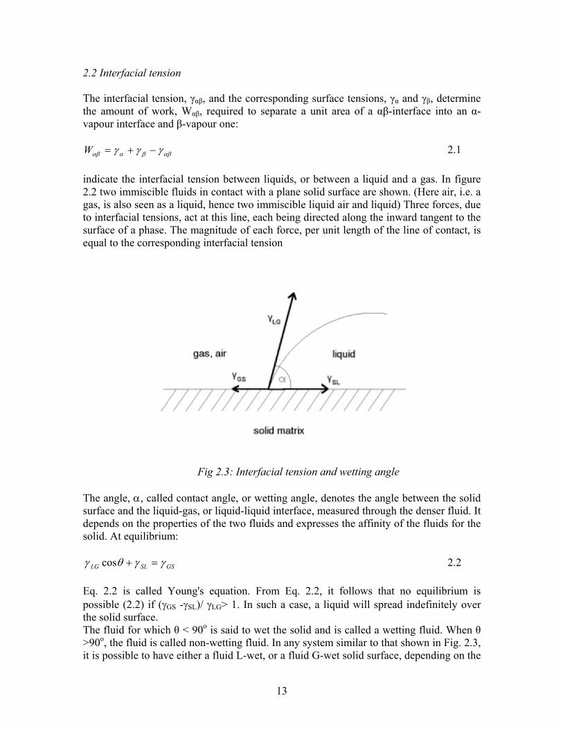
2.2 Interfacial tension The interfacial tension, γαβ, and the corresponding surface tensions, γα and γβ, determine the amount of work, Wαβ, required to separate a unit area of a αβ-interface into an α-vapour interface and β-vapour one:

αββααβ γγγ −+=W 2.1 indicate the interfacial tension between liquids, or between a liquid and a gas. In figure 2.2 two immiscible fluids in contact with a plane solid surface are shown. (Here air, i.e. a gas, is also seen as a liquid, hence two immiscible liquid air and liquid) Three forces, due to interfacial tensions, act at this line, each being directed along the inward tangent to the surface of a phase. The magnitude of each force, per unit length of the line of contact, is equal to the corresponding interfacial tension

Fig 2.3: Interfacial tension and wetting angle

The angle, α, called contact angle, or wetting angle, denotes the angle between the solid surface and the liquid-gas, or liquid-liquid interface, measured through the denser fluid. It depends on the properties of the two fluids and expresses the affinity of the fluids for the solid. At equilibrium:

GSSLLG γγθγ =+cos 2.2 Eq. 2.2 is called Young's equation. From Eq. 2.2, it follows that no equilibrium is possible (2.2) if (γGS -γSL)/ γLG> 1. In such a case, a liquid will spread indefinitely over the solid surface. The fluid for which θ < 90o is said to wet the solid and is called a wetting fluid. When θ >90o, the fluid is called non-wetting fluid. In any system similar to that shown in Fig. 2.3, it is possible to have either a fluid L-wet, or a fluid G-wet solid surface, depending on the

14

chemical composition of the two fluids and of the solid. In the unsaturated (air-water) zone in soil, water is, usually, the wetting phase, while air is the non-wetting one.

Figure 2.4 (a) The case of a liquid which wets a solid surface well, e.g. water on a very clean copper: perfect wetting (adhesion larger than cohesion). (b) The case of no wetting, contact angle =180o, e.g., water on teflon or mercury on clean glass (cohesion larger than adhesion).

θ 0° 90° 180°

cos θ 1 0 -1

Spreading Complete wett. Partial wetting γSL= γSV Negligible wett. Non-wett. (a) (b)

15

Thomas Young 1773-1829

Thomas Young's father was a banker and Young was brought up as a Quaker. He was a precocious child, learning to read by the age of two. He attended two boarding schools between 1780 and 1786 where his ability to learn languages became marked. He early also possessed extensive knowledge of mathematics, and natural sciences. In 1793 he entered St Bartholomew's Hospital, London, to study medicine. He continued this study at Edinburgh from 1794, and from 1795 in Göttingen. He obtained his medical doctorate in 1796. From 1797 to 1803 Young was attached to Emmanuel College Cambridge (MR 1803, MD 1808), where he turned his attention to scientific matters. In 1797 an uncle left him 10,000 pounds and a London house into which he moved in 1800 and in 1804 he married Eliza Maxwell. In 1799 Young set up a medical practice in London. His primary interest was in sense perception, and, while still a medical student, he had discovered the way in which the lens of the eye changes shape to focus on objects at differing distances. In 1801 he showed that astigmatism results from an improperly curved cornea. The same year he turned to the study of light. As early as around 1790, prior to the discovery of the cone cells in the retina, Young introduced the original theory of colour. What is now referred to as the Young-Helmholtz theory, was first published in 1802 by Thomas Young. It is based on the assumption that there are three fundamental colour sensations—red, green, and blue—and that there are three different groups of cones in the retina, each group particularly sensitive to one of these three colours. The theory was later further developed by Hermann von Helmholtz. In 1793 his paper On vision was read in the Royal Society and printed in its Transactions the same year. This occasioned his election to fellow of the same society in 1794, at the age of only 21 years. He received his doctorate at Göttingen in 1796, was accepted to the College at Cambridge, and was appointed professor of physics at the Royal Institution. By 1801, aged 28, Thomas Young was already professor of natural philosophy at the Royal Institution and lecturing on acoustics, optics, gravitation, astronomy, tides, the nature of heat, electricity, climate, animal life, vegetation, cohesion and capillary attraction of liquid, the hydrodynamics of reservoirs, canals and harbours, techniques of measurement, common forms of air and water pumps, and new ideas on energy. In 1802 Young became foreign secretary of the Royal Society, holding this position for the rest of his life. He was conferred doctor of medicine at Cambridge in 1808, and in 1809 was elected fellow of the College of Physicians. After his work on optics, Young returned to the study of languages, becoming particularly interested in Egyptology. From 1813 he started to attempt to decipher Egyptian hieroglyphics. Young began studying the texts of the Rosetta Stone in 1814. After obtaining additional hieroglyphic writings from other sources, he succeeded in providing a nearly accurate translation within a few years and thus contributed heavily to deciphering the ancient Egyptian language. From 1811 until his death he was physician at the St. George’s Hospital, however, without contributing anything of importance as a clinician. His medical works of 1813 and 1823 are mere compilations without any investigations of his own. Thomas Young died in London on 10 May 1829, and was buried in the cemetery of St. Giles Church in Farnborough, Kent, England. Westminster Abbey houses a white marble tablet in memory of Young bearing the epitaph by Hudson Gurney

16

2.3 Capillary pressure

A discontinuity in fluid pressure (actually, in fluid stress) exists across a curved interface that separates any two immiscible fluids (say, air and water). This is a consequence of the interfacial tension which exists at every point of such an interface. The difference between the pressure, pn, in the non-wetting phase, and that in the wetting one, pw, is called capillary pressure,

wnc ppp −= 2.3 where the pressures are taken in the two phases as the interface is approached from their respective sides.

The magnitude of the pressure difference at a point on an interface depends on the surface tension (= interfacial tension) and on the curvature of the latter at that point. There are several ways of deriving this relationship. In all of them, the interface is considered as a (two-dimensional) material body (actually, surface) which has rheological properties of its own. Its behavior is similar to a 'stretched membrane' under tension. In fact, this assumption alone already leads to the conclusion that under conditions of force equilibrium, the normal components of the fluid's stress, or pressure, must be discontinuous as a curved interface is crossed. As an example, we may make use of Fig. 2.4 that shows an infinitesimal element of a curved interface between a wetting fluid (w) and a non-wetting one (n).

Fig. 2.3 The force balance at a curved interface

Assuming the interfacial tension, γαβ, to be constant, a balance of force components normal to this element, at equilibrium, requires that

17

surface area

πr2

Surface tension along ring of 2 πr

Pc

Pc

wnwnwnc rrrppp γγ 211

21

=⎟⎟⎠

⎞⎜⎜⎝

⎛+=−= 2.4

where r1 and r2 are the two principal radii of curvature of the surface, and r* is the mean (2.4) radius of curvature defined by 2/r* = l/r1 + l/r2. Equation (2.4) is known as the Laplace formula for capillary pressure.

The simplest proof of capillary pressure

If we take a droplet and cut it in half Hence the force due to surface tension is:

γπ rF sionsurfaceten 2= whereas the force due to the capillary pressure is: ccapillary prF 2π= as there is no net movement, these forces should be equal and hence:

rpc

γ2=

18

2.4 Capillary

So far, we have been discussing the behavior of an interface at the microscopic level, i.e.,at a point on the curved interface (=meniscus) between two immiscible fluids within a pore. If the liquid completely wets the solid of which the wall of the tube is made, i.e., (θ = 0o), and the gas is the non-wetting fluid, the gas-liquid surface lies parallel to the wall and the interface must assume a concave shape (Fig. 2.5). If the capillary tube has a circular cross-section, with a radius, R, which is not too large, the curved interface (= meniscus) will, approximately, have the shape of a hemisphere. In this case, r* = r1= r2 = R. Similarly, when the liquid fails to wet the solid, i.e., θ = 180o, we observe a situation of capillary depression (Fig. 2.5), with a convex meniscus.

Fig 2.5: Two immiscible fluids with different contact angles in a capillary tube

In the general case, of a small diameter tube the pressure difference is given by:

rppp wn

wncθγ cos2

=−= 2.5

where pc is called the capillary pressure. This is also called the Washburn equation.

Due to the capillary pressure the moisture will rise in a tube. In equilibrium the capillary pressure is equal to the hydrostatic pressure, hence:

rgh

ργ2

max = 2.7

(For a fired-clay brick in which the pores are of the order of 1 μm the maximum capillary rise is 15 m)

19

3 Moisture in a porous material In the previous chapter we looked at capillary pressure in a single. In this chapter we will look at water distribution in porous materials which contain a (broad) range of pore sizes. Finally attention will be given to the relative humidity in a porous material 3.1 Capillary pressure curves In analogy with the definition of capillary pressure at the microscopic level we can define an average pressure within each of the two fluid phases at the macroscopic level:

wnc ppp −= 3.1 It is often assumed that the air is at a constant, atmospheric, pressure, taken as zero, i.e.,

wc pp −= 3.2

However in porous materials there will be a distribution of pore sizes. Therefore, not all pores will empty/fill at the same capillary pressure. The large pores (or those with larger channels, or throats of entry) will empty at low capillary pressures, while those with narrow channels of entry will empty at higher capillary pressures.

Figure 3.1 Gradual drainage and wetting: at each pressure there will be a local equilibrium

If at some point in time, the drainage/wetting of the wetting fluid of the sample is

stopped, an equilibrium situation will be established after a while. With no further fluid motion, the pressure distribution within each fluid will be hydrostatic, while satisfying the pressure jump conditions at every point of the (microscopic) interfaces. At each of

20

these points, the pressure jump will correspond to the radius of curvature of the interface at that point, see figure 3.1.

It is obvious that at each stage of a drainage/wetting process, the quantity of wetting fluid remaining, say, within a certain REV, adopts a certain (microscopic) configuration. The latter is related to the distribution of the (microscopic) capillary pressure at all points of the interface within that REV. Hence the capillary pressure will be a function of the moisture content, θ:

)(θcc pp = 3.3 Often, however, in stead of the capillary pressure the suction is given, which is defined as:

ρθ

ψg

pc )(= 3.4

Hence the suction, ψ, is now expressed in meters.

In figure 3.2 an example is given of a typical capillary pressure curve. Upon wetting or draining two different curves are measured.

Figure 3.2: Schematic diagram of a capillary pressure curve for a porous material. (Only the main curves for drying and wetting are given. Each point on these curves represents an equilibrium situation with no liquid transport). In general for a given porous material and fluid(s), the capillary pressure curve has to be derived experimentally, using available instruments. It is important to emphasize that the experiments are performed such that each point on the curve represents an equilibrium situation, with no fluid motion.

21

3.2 Hysteresis The phenomenon of dependence of the curve upon the history of drainage and wetting of a sample, is called hysteresis. It is attributed to a number of causes. The ink-bottle effect results from the shape of the pores with changing wide and narrow passages. In such a nonuniform capillary there is a bi-stability of the interface. Wetting an initially dry or drying an initially wet capillary gives rise to two different stable configurations of the liquid (see Fig. 3.3a). These two configurations differ in moisture content. In a porous medium which contains a wide range of pores with different dimensions and shapes many stable configurations are possible, all contributing to the hysteresis. Another effect, the raindrop effect, represents the different contact-angle for an advancing and a receding water front at a solid-liquid interface, as is indicated by the shape of a raindrop (see Fig. 3.3b). This effect may be due to contamination of either the fluid or the surface, possible variability of the minerals that compose the surface, and surface roughness. A third effect is air entrapment in a porous medium after draining or rewetting (see Fig. 3.2). As a result the moisture content will only raise, under atmospheric conditions, to the so-called capillary moisture content, θcap. The entrapped air is generally assumed to be present in the dead-end pores, and hence θcap≈neff . Analytic expressions are available to describe the effect of hysteresis in the capillary pressure curve. These are generally based on the so-called independent domain model, e.g., [MUA73, MUA74].

Figure: 3.3 Schematic representations of two effects contributing to hysteresis. a) The

inkbottle effect results from the non-uniform width of the pores. Wetting an initially dry or drying an initially wet capillary, gives rise to two different stable configurations. b)

The raindrop effect represents the different contact-angle for an advancing and a receding water front at the solid-liquid interface.

As s result of hysteresis the complete history has to be know in order to know the capillary pressure/ moisture content

22

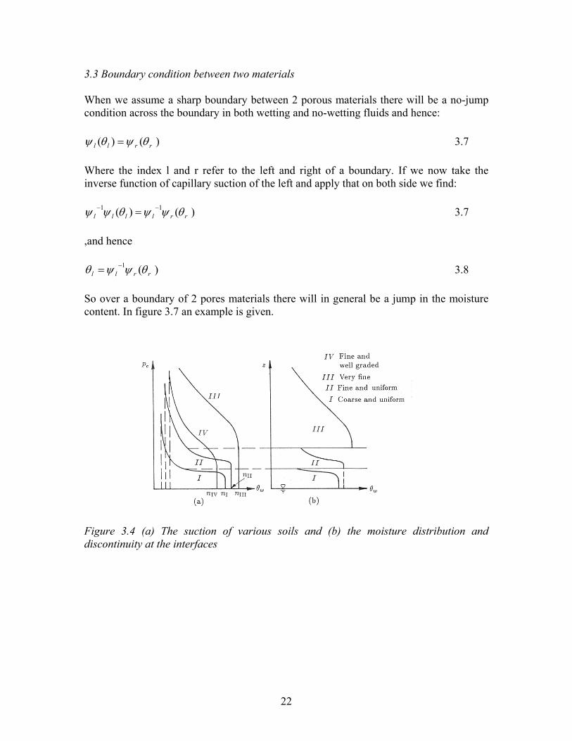
3.3 Boundary condition between two materials When we assume a sharp boundary between 2 porous materials there will be a no-jump condition across the boundary in both wetting and no-wetting fluids and hence:

)()( rrll θψθψ = 3.7 Where the index l and r refer to the left and right of a boundary. If we now take the inverse function of capillary suction of the left and apply that on both side we find:

)()( 11rrllll θψψθψψ −− = 3.7

,and hence

)(1rrll θψψθ −= 3.8

So over a boundary of 2 pores materials there will in general be a jump in the moisture content. In figure 3.7 an example is given. Figure 3.4 (a) The suction of various soils and (b) the moisture distribution and discontinuity at the interfaces

23

3.4 Sorption isotherm/hygroscopic curve

Above a curved interface there will be equilibrium between a liquid and its vapour. This equilibrium depends on the curvature of the liquid- (vapour containing) gas interface. The relative humidity h above a curved interface is given by:

⎟⎟⎠

⎞⎜⎜⎝

⎛ −==

RTrpph l

vs

v

ργ2exp 3.9

Here pvs the saturation pressure of water above a flat surface. This is better known as Kelvin's law/ Thomson's law. (Hence in a small capillary, water will condense until equilibrium is established with the surrounding relative humidity of the air). In figure 3.5 the maximum relative humidity is given as a function of pore size

Figure 3.5 The maximum relative humidity as function of pore radius in a pore

Also in a porous material there will be an equilibrium between the water and its vapour. Locally, within a pore, this equilibrium depends on the curvature of the liquid/gas interface. Assuming some average capillary pressure, Edelfsen and Anderson [EDF43] have shown that at the macroscopic level:

⎟⎠⎞

⎜⎝⎛== ψ

RTMg

pp

hvs

v exp 3.10

The curves obtained by measuring the moisture content as a function of the

relative humidity are called sorption isotherm or hygroscopic curves. These will also show a hysteresis. In figure 3.7 examples are given of the measured hygroscopic curves for various materials.

24

Figure 3.7: Hygroscopic curves; the main curves for absorption and desorption measured for fired-clay brick (• ), sand-lime brick ( , ), gypsum ( , ) and mortar (

, ). 3.7 Measurement of capillary pressure curve/ sorption isotherm Capillary pressure curve

The capillary pressure curve is measured by placing a sample on a semi-permeable membrane in a closed sample room. This membrane allows water to pass through but is air tight. By slowly increasing and decreasing the air pressure in the sample room the capillary pressure can be varied. As each point on such a curve represents equilibrium situation where no moisture transport occurs it takes on average 1 to 2 weeks for a sample to reach equilibrium at each measurement point. Sorption isotherm

The sorption isotherms are measured by bringing a sample in contact with air having a certain relative humidity and waiting for equilibrium. For the sorption curve an initially dry sample is used and for the desorption curve an initially wet sample. The different relative humidity’s are generally created by saturated salt solutions. Again, as each point on such a curve represents equilibrium situation where no moisture transport occurs, it takes on average 3 to 4 weeks for a sample to reach equilibrium at each measurement point.

25

Fig 3.7: The experimental set-up for measuring the capillary pressure curve Thermodynamic derivation of capillary condensation This pressure is given by:

rpp lv

γ2=−

Therefore applies:

rddpdp lv

12λ=− (*)

By use of the Gibbs Duhem equation, an expression for dpi in which i is the phase can be written: dμl =υl dpl and dμv =υv dpv . Because of equilibrium the chemical potential (μ ) is the same for both phases. If the equilibrium is shifted slowly the system will stay in equilibrium therefore dμl = dμv . This results in:

vl

vl dp

vv

dp ⎟⎟⎠

⎞⎜⎜⎝

⎛=

Then equation (*) can be written as:

rddp

vv

vl

v 121 λ=⎟⎟⎠

⎞⎜⎜⎝

⎛⎟⎟⎠

⎞⎜⎜⎝

⎛−

After rewetting this is:

∫∫ =⎟⎟⎠

⎞⎜⎜⎝

⎛ − r

v

p

p l

vl

rddp

vvv

o 0

12λ

Now we assume the vapor to behave as an ideal gas (vvpv=RT). We neglect the molar volume of the liquid compared to the molar volume of the gas (for water 1 mol of vapor is 22 l, whereas 1 mol of liquid is 0.018l) resulting in:

∫∫ =⎟⎟⎠

⎞⎜⎜⎝

⎛ r

v

p

p vl rddp

pvRT

o 0

12λ

After assuming that the liquid is incompressible this can be integrated resulting in:

rpp

vRT

ol

γ2ln =

This equation shows that at relative humidity (p/p0) in a pore of radius r condensation takes place. In other words; the humidity needed for condensation is below the saturation humidity (below 100%).

26

4 Saturated transport In this chapter we will take a look at the transport through a fully saturated porous material, introducing the law of Darcy [DAR57]. Based on this by Dupuit an approximation was introduced by which various engineering problems could be solved. 4.1 Darcy law The volume rate [m3/s] through a cylinder with radius r and length l is given by Poisseuille's law:

4( )8

o lcyl

p p rQl

πμ

−= 4.1

where Δp is the pressure difference over the cylinder, ρ the density and μ the viscosity of the liquid. If we now model a saturated porous medium as a bundle of capillary tubes the flux through a porous material is given (see figure 4.1): 4.2 Figure 5.1: Schematic representation of the flow through a fully saturated porous material. However in a porous material the flow will not be in a direct line but through a tortuous way. Therefore a correction factor, so-called tortuosity T, is introduced to account for the increased length;

V1 V2

po

pl

μ8)(

2i

ilotot

r

lTpp

Q∑−

=

27

4

( )8

io l i

tot

rp pQ

T l

π

μ−

=∑

4.3

Therefor the volume flux through a porous material per unit area will be: 4.4 And hence the flux, i.e., volume flux per area, for a porous material is given by: 4.5 In a more general way this can be rewritten for a porous material as:

xpkq∂∂

−=μ

4.6

This equation is better known as Darcy's law, where k is called the permeability of a porous medium. (So Darcy's law is a simple linear transport law, having exactly the same from as Ohm's law and Fick's law). Darcy's law describes the flow through a porous medium as function of the applied pressure. (Here a more phenomenological way was taken to derive Darcy's law. However, one can also derive this Darcy law by volume averaging the condition of momentum conservation, see e.g., BEA 90). It is very common to express the pressure in the suction, i.e.;

gpρ

ψ = 4.7

Hence Darcy's law can be rewritten as:

xKq

∂∂

−=ψ 4.8

where K is the effective hydraulic conductivity (which is now dependent on the liquid properties):

μρgkK = 4.9

μ8)(

2i

ilotot

r

lTpp

Q∑−

=

μ8)(

2i

i

porous

lotot

r

lTApp

q∑−

=

28

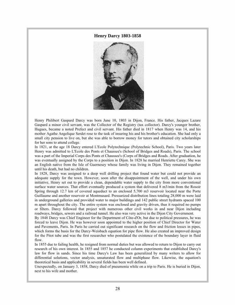
Henry Darcy 1803-1858

Henry Philibert Gaspard Darcy was born June 10, 1803 in Dijon, France. His father, Jacques Lazare Gaspard a minor civil servant, was the Collector of the Registry (tax collector). Darcy's younger brother, Hugues, became a noted Prefect and civil servant. His father died in 1817 when Henry was 14, and his mother Agathe Angelique Serdet rose to the task of insuring his and his brother's education. She had only a small city pension to live on, but she was able to borrow money for tutors and obtained city scholarships for her sons to attend college. In 1821, at the age 18 Darcy entered L'Ecole Polytechnique (Polytechnic School), Paris. Two years later Henry was admitted to L'Ecole des Ponts et Chaussee's (School of Bridges and Roads), Paris. The school was a part of the Imperial Corps des Ponts et Chaussee's (Corps of Bridges and Roads. After graduation, he was eventually assigned by the Corps to a position in Dijon. In 1828 he married Henriette Carey. She was an English native from the Isle of Guernesey whose family was living in Dijon. They remained together until his death, but had no children. In 1828, Darcy was assigned to a deep well drilling project that found water but could not provide an adequate supply for the town. However, soon after the disappointment of the well, and under his own initiative, Henry set out to provide a clean, dependable water supply to the city from more conventional surface water sources. That effort eventually produced a system that delivered 8 m3/min from the Rosoir Spring through 12.7 km of covered aqueduct to an enclosed 5,700 m3 reservoir located near the Porte Guillaume and another reservoir at Montmusard. Pressurized distribution lines totaling 28,000 m were laid in underground galleries and provided water to major buildings and 142 public street hydrants spaced 100 m apart throughout the city. The entire system was enclosed and gravity driven, thus it required no pumps or filters. Darcy followed that project with numerous other civil works in and near Dijon including roadways, bridges, sewers and a railroad tunnel. He also was very active in the Dijon City Government. By 1848 Darcy was Chief Engineer for the Department of Côte-d'Or, but due to political pressures, he was forced to leave Dijon. He was however soon appointed to the higher position of Chief Director for Water and Pavements, Paris. In Paris he carried out significant research on the flow and friction losses in pipes, which forms the basis for the Darcy-Weisbach equation for pipe flow. He also created an improved design for the Pitot tube and was the first researcher who postulated the existence of the boundary layer in fluid flow. In 1855 due to failing health, he resigned from normal duties but was allowed to return to Dijon to carry out research of his own interest. In 1855 and 1857 he conducted column experiments that established Darcy's law for flow in sands. Since his time Darcy's Law has been generalized by many writers to allow for differential solutions, vector analysis, unsaturated flow and multiphase flow. Likewise, the equation's theoretical basis and applicability in several fields has been well defined. Unexpectedly, on January 3, 1858, Darcy died of pneumonia while on a trip to Paris. He is buried in Dijon, next to his wife and mother.

29

Examples of the K of various materials: Fired-clay brick = 2.5x10-7 ms-1 Cement paste = 4.0x10-7 ms-1 High strength concrete = 7.7x10-13 ms-1 Darcy unit Permeability has units of m2, but in petroleum engineering it is conventional to use “Darcy” units, defined by ; 1Darcy = 0.987 ×10−12 m2 ≈ 10−12 m2 . The Darcy unit is defined such that a rock having a permeability of 1 Darcy would transmit 1 cc of water (with viscosity 1 cP) per second, through a region of 1 sq. cm. cross-sectional area, if the pressure drop along the direction of flow were 1 atm per cm. Many soils and sands that civil engineers must deal with have permeabilities on the order of a few Darcies. The original purpose of the “Darcy” definition was therefore to avoid the need for using small prefixes such as 10-12, etc. It is important to realize there is no-direct relaxation between porosity and permeability. As an example in figure 5.1 the measured permeability is given as a function of porosity for various materials.

Figure 4.2 The measured permeability as a function of the porosity (Darcy : 9.8792 10-13 m2)

30

4.2 Continuity The macroscopic conservation of mass for liquid water expressed in volumetric quantities can be written as:

0. =∇+∂∂ q

tθ 4.10

Since for a saturated porous materials n=θ=constant this equation reduces to:

0. =∇ q 4.11 Hence combining with Eq 4.7 the flow in a homogeneous porous material can now be described by:

02 =∇ ψ 4.12 That is by the well known Laplace equation. 4.2 Dupuit approximation In practice most engineering problem are 2D/3D and can not be solved without computer simulations. By Dupuit an approximation was developed, which is a very powerful tool for engineers and hydrologists, to solve problem relating to unconfined flows.

Figure 4.3 A schematic representation of the Dupuit approximation

31X = 0 X = L X

h1

h2

Dupuit observed that very often in an unconfined aquifer the water table is also the upper boundary of the region of flow. Hence he assumed:

- The hydraulic gradient equals the slope of the water table - For small water-table gradients, the flow lines are horizontal and the equipotential

lines are vertical Hence Darcy’s equation can in this case be approximated by:

xhKq∂∂

−= 4.13

So a basically 2D problem can be approximated as a 1D problem 4.3 Flow between two reservoirs As an example the discharge between two reservoirs can be calculated (see figure 4.4) . The total volume flux Q at any position is now given by:

dxdhKhQ −= 4.14

Where h is the saturated thickness with boundary conditions x=0, h=h1 and x=L, h=h2 . Integrating eq. 4.13 with these boundary conditions gives:

xhh

KQ x

2)( 22

1 −−= 4.15

Incorperating the boundary condition x=L and taking into account that Q=constant, one can now derive an expression for the water table:

Lhhxhhx

)( 21

222

12 −

+= 4.16

which is known as the Dupuit parabola. If one does an exact calculation it is interesting that although the shape of the water table is only an approximation that the discharge as given by 4.14 is still correct, hence this indicates why the Dupuit approximation is a powerful tool for engineers.

32

Figure 4.4 : The discharge between two reservoirs

Jules Dupuit was perhaps the most illustrious of the French engineer-economists. Trained at the École des Ponts et Chaussées in Paris, Dupuit had a distinguished career as a civil engineer. Starting out as chief engineer in the Sarthe region, Dupuit wrote several first-class theoretical and practical studies of road deterioration and maintenance (1837, 1842), for which he earned a Légion d'honneur in 1843. His studies on flood management (1848), drawn from his experience in the Loire, also made a big impression. Engineering questions led into his seminal contributions to economics. His 1844 articles was concerned with the find the toll that should be charged on a bridge. It was here that he introduced his curve of diminishing marginal utility and suggested that, the higher the toll, the lower. Dupuit was called to Paris in 1850 and made chief engineer. It was here that he made he studies of municipal water systems and hydraulics and supervised the construction of the Paris sewer system. In 1855, he was named inspector general of the Corps des Ingénieurs and served on the Conseil des Ponts et Chaussées until his death.

33

5 Unsaturated transport: Liquid transport In this chapter we will look at the moisture transport in an unsaturated porous material, i.e., water and air. First we will consider the absorption in a capillary tube followed by a more general description of the unsaturated liquid transport in a porous material. Finally, we will look at the water absorption in a porous material 5.1 Absorption in a capillary In an oversimplified view, one can see a porous medium absorbing a fluid as a capillary tube in which water is absorbed. Due to the curved surface there will be a capillary pressure, which is given by:

rpc

γ2−= 5.1

The flow through a capillary tube is given by Poisseuille law:

2( )8

o lp p rvl μ−

= 5.2

Combining Eq. 7.1 and 7.2 one obtains (see also figure 7.3):

μ8

2rxp

dtdx Δ

= 5.3

where X is the position of the front (see also figure 7.3) Therefore the position of the front is given by:

trxμγ2

= 5.4

So the position of the wetting front is proportional to the square root out of time. This general behaviour is indeed observed in porous materials. (Be aware that we have made a fundamental choice in this calculation, i.e., there is no air flow)

Fig 5.1: Schematic representation of the absorption in a capillary

34

5.2 Liquid transport in porous material In analogy to a saturated porous medium, the liquid water transport in a non-saturated medium is described by Darcy's law:

)()( θμθ

cpkq ∇−= 5.5

where kl(θl) is the effective permeability for liquid water, which now depends on the moisture content. Liquid water is now transported because of inhomogeneities in capillary action. Equation 5.5 can be rewritten as:

)()( θψθ ∇−= Kq 5.7 where

μρθ gkK )(

= 5.7

is the hydraulic conductivity which is a function of the moisture content and is the suction. Under isothermal conditions the suction only varies with the moisture content, and equation can be rewritten as:

θθ ∇−= )(Dq 5.8 where

T

KD ⎟⎠⎞

⎜⎝⎛∂∂

=θψθ )( 5.9

is so-called the isothermal liquid diffusivity. (Comparison with Fick's law of molecular diffusion explains the term 'diffusivity' for D) The macroscopic conservation of mass for liquid water expressed in volumetric quantities can be written as:

0. =∇+∂∂ q

tθ 5.10

Combining equation 5.9 and 5.10, the liquid moisture transport can be described as a non-linear diffusion equation:

( )θθθ∇∇=

∂∂ )(D

t 5.11

35

5.3 Water absorption In case of a semi one-dimensional absorption experiment, Eq. 5.11 can be rewritten as:

⎟⎠⎞

⎜⎝⎛

∂∂

∂∂

=∂∂

xD

xtθθ 5.12

During absorption we have the initial and boundary conditions:

0,00,00>===>=txat

txfor

capθθθ

5.14

In these conditions θcap is the capillary moisture content, which is the maximum moisture content under atmospheric conditions, and θo is the initial uniform moisture content of the sample. If the so-called Boltzmann transformation:

tx

=λ 5.15

is applied, the non-linear diffusion equation (5.12) describing the moisture transport reduces to the ordinary differential equation:

02 =+⎟⎠⎞

⎜⎝⎛

λθλ

λθ

λ dd

ddD

dd 5.17A

with boundary conditions:

00

==∞→=

λθθλθ

atfor

cap 5.17B

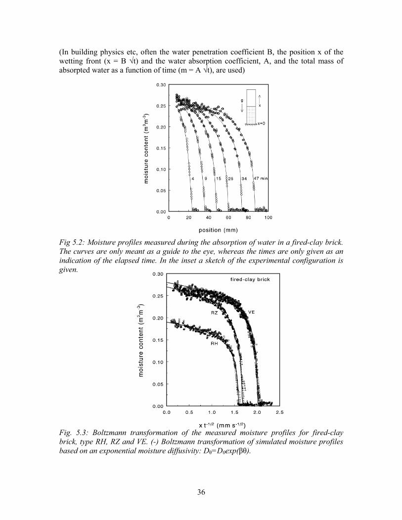
Equation 5.17A with boundary conditions 5.17B has only one solution, so the profiles during water absorption at different times are related by a simple √t scaling. (BE AWARE: Some people conclude from the fact that both a simple calculation and a more fundamental calculation give the same result they can always model a porous material with a simple capillary. However, this is completely wrong: It is a pure coincidence that in this case both of these calculations give a √t behaviour.) An example of the measured moisture profiles as measured with NMR-imaging during the absorption of water in fired-clay brick is given in figure 5.2. As can be seen from these moisture profiles a very steep wetting front is formed. In figure 5.3 the Boltzmann transformation of the measured moisture profiles are given. As can be seen all profiles for a certain material collapse on one master curve, indicating that indeed all profiles scale with √t. This also indicates that the moisture diffusivity does not depend on the position and supports the modeling of the moisture transport during absorption in porous materials by a diffusion equation.

36

(In building physics etc, often the water penetration coefficient B, the position x of the wetting front (x = B √t) and the water absorption coefficient, A, and the total mass of absorpted water as a function of time (m = A √t), are used) Fig 5.2: Moisture profiles measured during the absorption of water in a fired-clay brick. The curves are only meant as a guide to the eye, whereas the times are only given as an indication of the elapsed time. In the inset a sketch of the experimental configuration is given. Fig. 5.3: Boltzmann transformation of the measured moisture profiles for fired-clay brick, type RH, RZ and VE. (-) Boltzmann transformation of simulated moisture profiles based on an exponential moisture diffusivity: Dθ=D0exp(βθ).

37

5.4 Liquid moisture diffusivity In principle, the moisture diffusivity for absorption can be determined from experimental data by integrating equation 5.17 with respect to λ using the boundary conditions 5.17, yielding:

∫⎟⎠⎞

⎜⎝⎛

−=θ

θ

θλ

λθ 0

'121 d

dd

D 5.18

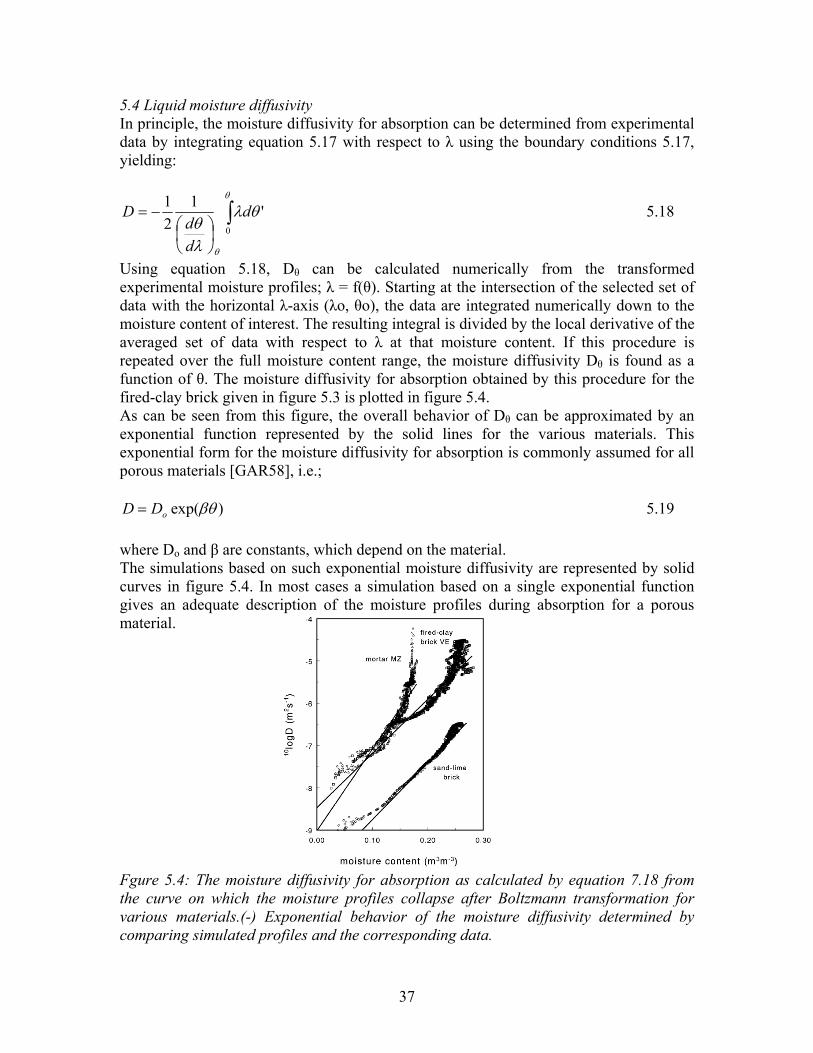
Using equation 5.18, Dθ can be calculated numerically from the transformed experimental moisture profiles; λ = f(θ). Starting at the intersection of the selected set of data with the horizontal λ-axis (λo, θo), the data are integrated numerically down to the moisture content of interest. The resulting integral is divided by the local derivative of the averaged set of data with respect to λ at that moisture content. If this procedure is repeated over the full moisture content range, the moisture diffusivity Dθ is found as a function of θ. The moisture diffusivity for absorption obtained by this procedure for the fired-clay brick given in figure 5.3 is plotted in figure 5.4. As can be seen from this figure, the overall behavior of Dθ can be approximated by an exponential function represented by the solid lines for the various materials. This exponential form for the moisture diffusivity for absorption is commonly assumed for all porous materials [GAR58], i.e.;

)exp(βθoDD = 5.19 where Do and β are constants, which depend on the material. The simulations based on such exponential moisture diffusivity are represented by solid curves in figure 5.4. In most cases a simulation based on a single exponential function gives an adequate description of the moisture profiles during absorption for a porous material. Fgure 5.4: The moisture diffusivity for absorption as calculated by equation 7.18 from the curve on which the moisture profiles collapse after Boltzmann transformation for various materials.(-) Exponential behavior of the moisture diffusivity determined by comparing simulated profiles and the corresponding data.

38

Brick laying: craftsmanship needed

The water extraction out of mortars that occurs during brick laying is an important parameter determining, e.g., the stiffness of the mortar due to compaction of cement particles and aggregate grains and the bond strength of the cured brick-mortar interface. Brick laying seems a simple process but it requires real craftsmanship. In order to understand this we will have a closer look at the moisture transport. Regarding the water extraction out of mortar, both the water absorption rate and the suction of the brick are important factors. Here we will take two materials: a fired-clay brick and a sand-lime brick: a sand-lime brick has more small pores, and hence a lower absorption rate than a fired-clay brick. But it also has a ‘suction' due to the small pores, which is directly related to the lower 'absorption rate'. In the figure the results are presented for both types of brick. The dashed curves indicate the initial moisture profiles in the brick and the mortar. The shaded area indicates the boundary area. As the one-dimensional resolution of our instrument is 1 mm, the moisture profiles in this area are only given as a guide to the eye; the actual moisture profiles may be steeper. The moisture profiles as measured during absorption of moisture out of the same mortar. The profiles were measured every 90sec As can be seen the moisture profiles in the mortar remain rather flat during the water extraction process, indicating that the moisture diffusivity for liquid water in the mortar is larger than that in the bricks at these moisture contents. It is evident that most of the water is extracted out of the mortar within the first 90 seconds. In the case of fired-clay brick almost stationary moisture content in the mortar is reached within 3 min, whereas in the case of sand-lime brick this takes about 10 min. The difference in suction is reflected in the final moisture content reached in the mortar. Hence with brick laying you have only one chance to do it correctly. This makes that craftsmanship is needed.

39

6 Unsaturated transport: combined liquid and vapour transport In this chapter we will look at the vapour transport in unsaturated porous materials. First the concept of critical moisture content will be introduced. We will then derive a general description of the vapour transport in a porous material. However, in general there will be a combination/interaction of vapour and liquid transport, which will be discussed. Finally, as an example we will consider the drying of a porous material. 6.1 Critical moisture content In figure 6.1, schematically, the magnitude of the force of molecular attraction between a solid and a wetting fluid is given. This force decreases rapidly with the distance from the solid wall. In the first two sublayers, the so-called adhesive fluid layer, the forces are significant. When the fluid is water the water molecules are oriented perpendicular to the solid surface because of their bipolar structure. The stress created by the attractive forces is very strong. In this layer, the properties of the fluid differ significantly from those of ordinary water, e.g., the density and viscosity are much larger. The second sublayer of adhesive fluid (from 0.1 to 0.5 μm in water), forms a transition zone in which the forces of attraction still play a role in making the fluid in this layer practically immobile. Further away from the solid, the fluid is said to be free, or mobile. Figure 6.1 Schematic diagram of the force acting on the water molecules near a surface. To obtain more insight about the distribution of fluids within the void space consider the case of air (= non-wetting fluid) and water (= wetting fluid) in a porous medium. At low saturations (see Fig. 6.2), water will only be present at the surface in an immobile layer. Increasing the moisture content these layers will become thicker. At the so-called critical moisture content these water layers will make contact and a continuous water phase is formed. Above this point water can be transported by fluid transport, i.e., in general: θ < θcritical : vapour transport dominant θ > θcritical : liquid transport dominant

40

Figure 6.2 Schematic filling of a porous material with water.

6.2 Vapour transport At the microscopic level the vapour transport under isothermal conditions is given by Fick's law:

vvl

v pDRTMq ∇=

ρ1 6.1

In this equation Dv is the diffusion coefficient of water vapour in air, M the molecular mass of water, R the gas constant, T the absolute temperature, and pv the vapour pressure. The term M/RT results from the ideal gas law, whereas ρl results from the transformation of the mass flux for vapour into an equivalent volumetric liquid water flux. By Bear [BEA90] it has been shown that by volume averaging the local macroscopic gradient of a function f can be related to the microscopic gradient of the function f according to:

∫+∇=∇ FdsFTF * 6.2 In this equation T* is the so-called tortuosity and the second part is a surface integral. Neglecting the surface sink, by volume averaging of equation 6.1 the macroscopic volumetric flux through a porous medium with only air and vapour (n = θv+θa ) is obtained:

vvl

v pDTRTMnq ∇= *

ρ 6.3

In the case of vapour transport the tortuosity is often considered as accounting for the extra path length resulting from the tortuous pore system. In case of a non-saturated porous medium, the macroscopic vapour transport is given by:

vvll

lv pDT

RTMn

q ∇−

= )(* θρθ

6.4

41

The tortuosity is now related to the void-space available for vapour diffusion (θv+θa= n- θl )and is therefore a function of the liquid water content. The macroscopic capillary pressure is related to the macroscopic vapour pressure by (see section 3.4):

⎟⎠⎞

⎜⎝⎛== )(exp θψ

RTMg

pp

hvs

v 6.5

This equation shows that, under isothermal conditions, the relative humidity only varies with the suction and thereby with the moisture content θl. Therefore the gradient of the vapour pressure can be rewritten as:

lT

vsvhpp θθ

∇⎟⎠⎞

⎜⎝⎛∂∂

=∇ 6.7

Combining equations 6.4, 6.5, 6.7, and using the ideal gas law, the vapour transport can be rewritten as:

lvv Dq θ∇= 6.7 where

Tlvl

l

vlv DT

RTMgnD ⎟⎟

⎠

⎞⎜⎜⎝

⎛∂∂

−=θψθ

ρρ

θ )()( * 6.8

is the isothermal vapour diffusivity (by diffusion only). In experiments, however, it is observed that the actual vapour flux is much larger than that predicted by equation 6.6 and 6.8 on basis of Fick's law. Various models have been introduced to account for this enhancement, i.e., the liquid island model [PHI57], surface diffusion [STA86, CHE89], surface flow [ROW71], and surface hopping [OKA81]. For example, Philip and de Vries [PHI57] developed a microscopic model to account for the enhancement based on liquid islands. They suggested that in a porous material water islands will be formed due to capillary condensation. If over such an island a vapour gradient is present, vapour will condensate at one end of this island. At the same time water has to evaporate at the other side to maintain equilibrium. The water will pass the island by a much faster mechanism: liquid transport. As a consequence, the diffusion coefficient will increase. It is generally assumed that for the various vapour enhancement mechanisms the contribution to the macroscopic vapour flux is in first order proportional to the gradient of the liquid water content. Hence the macroscopic vapour flux can be rewritten as:

lvv Dq θ∇= 6.9 where Dθ,v is called the isothermal vapour diffusivity. In this coefficient all enhancement mechanisms are taken into account, i.e.,;

42

idealvsurfaceislandsv DD ,)1( αα ++= 6.10 In general this coefficient has to be determined experimentally for the porous medium of interest. Figure 6.1 A schematic representation of two mechanisms for vapour diffusion enhancement. In the water island model, water vapour condensates at one end of a liquid island and at the same time water evaporates at the other side to maintain equilibrium. By surface diffusion water will be transported along the pore wall. 6.2 Combined moisture and vapour transport In case of a combined moisture and vapour transport the mass balance equation on the macroscopic scale for water vapour in volumetric quantities is given by:

Eqt vv +∇=

∂∂

.θ

6.11

where Ev→l is the rate of condensation . Combining equations 6.9 and 6.10 the vapour transport can be described by:

++∇∇=∂∂

EDt llvv ))(.( θθ

θ 6.12

Taking into account the evaporation (Ev→l = El→v) the liquid transport can be described by:

−−∇∇=∂∂

EDt lll

l ))(.( θθθ

6.13

43

Combining equations 6.10 and 6.12, describing the liquid and vapour transport respectively, the moisture transport can be written as:

))(.()(

lllv D

tθθ

θθ∇∇=

∂+∂

6.14

where

)()()( lllvl DDD θθθ += 6.15 is called the isothermal moisture diffusivity. Assuming equilibrium between water and vapour, the mass density of the vapour in the pores is given by:

l

lvv n θ

ρθρ

−= 6.17

Hence, the moisture content can be written as:

ll

v

l

vlv n θ

ρρ

ρρ

θθθ ⎟⎟⎠

⎞⎜⎜⎝

⎛−+⎟⎟

⎠

⎞⎜⎜⎝

⎛=+= 1 6.17

Since ρv is of the order of 10-5 ρl , the right hand side of Eq. 6.17 is to a good approximation equal to θl for liquid water contents larger than 10-3. Hence, the moisture transport in a porous medium can be approximated by a non-linear diffusion equation:

))(.( θθθ

∇∇=∂

∂D

t 6.18

6.3 Drying experiment The most general example of unsaturated transport is the drying of a material. In figure 6.2 a drying experiment is illustrated as performed using NMR. The sample, a small cylinder with a length of 25 mm and a diameter of 20 mm, is placed in a teflon holder of which the upper side is open (teflon does hardly contain any hydrogen). Air, with a 45 ± 5 % relative humidity (RH) and a temperature of 293 ± 0.5 K, is blown over the sample, thus creating a one-dimensional drying experiment.

44

Figure 6.2 Experimental probe head for measuring moisture profiles during drying using NMR. In figure 6.3 an example of the measured moisture profiles are given for a fired-clay brick. The variations reproduced from profile to profile, e.g., at a position of 5 mm, reflect the inhomogeneities of the sample. In the beginning the moisture profiles are almost flat reflecting a high moisture diffusivity, i.e, liquid water transport. A drying front entering the material is observed after approximately 7 hours, i.e., the critical moisture content has been reached. At this stage water has first to evaporate and next to be transported by vapour transport. Figure 6.3 Moisture profiles measured during drying for fired-clay brick. The time between subsequent profiles is 1 hour and the profiles are given for a period of 42 hours.

45

Under isothermal conditions the flux across the boundary material/air is given by:

)( materialair hhq −= β 6.19 where n is the unit vector normal to the material/air interface, β the mass transfer coefficient, ha the relative humidity of the air, and hm the relative humidity of the material at the interface. The mass transfer coefficient depends on many parameters, such as air velocity, porosity, and surface roughness. In general, this coefficient has to be determined experimentally [ILL52]. In case the mass transfer coefficient is large, as in this experiment, 6.19 can be approximated by:

)(.. θhygroairmaterialair fheihh == 6.20 Hence in this case the final moisture content which can be reached is given by the corresponding hygroscopic moisture content. 6.4 The moisture diffusivity To derive Dθ from the experimental moisture profiles, equation 6.15 is integrated with respect to x, yielding:

'

'

)(

x

x

l

x

dxt

D⎟⎠⎞

⎜⎝⎛∂∂

⎟⎠⎞

⎜⎝⎛∂∂

=∫

θ

θ

θ 6.21

In this equation, use is made of the fact that the partial derivative of θ with respect to x is zero at the vapour tight bottom (x = l). The resulting numerically calculated moisture diffusivity is given in figure 6.4. In this figure only results are included for those regions of the material where the effects of inhomogeneities are relatively small and the situation can be regarded as isothermal. For the calculations of the derivative ∂θ/∂x local averages of the experimental data were taken, to reduce the effect of fluctuations. It is obvious that the data in the figure have a significant scatter, which is rather pronounced at both high and low moisture contents. This is directly related to the accuracy by which the derivative of the moisture content with respect to position can be determined. Despite these uncertainties, the data clearly reveal a well defined variation of the moisture diffusivity with moisture content, indicating that the moisture diffusivity does not depend upon the position. This indicates that also the combined moisture and vapour transport during drying in these materials can be modeled by a diffusion equation. In the observed behaviour of the moisture diffusivity three regimes can be distinguished, which each can be related to a certain regions of the moisture profiles (see Fig. 6.3). At

46

high moisture contents the moisture transport is dominated by liquid transport: the almost horizontal profiles correspond to high moisture diffusivity. With decreasing moisture content the large pores will be drained and will therefore no longer contribute to liquid transport. Consequently the moisture diffusivity will decrease. Below the critical moisture content, the water in the sample no longer forms a continuous phase. Hence the moisture has to be transported by vapour and this transport will therefore be governed by the vapour pressure. For small moisture contents the moisture diffusivity starts to increase again, resulting in a minimum in the moisture diffusivity. This can be explained by noting that the contribution of the vapour transport to the moisture transport can be related to the slope ∂θ/∂RH of the hygroscopic curve. (see figure 3.3) Starting at 100 % relative humidity the slope decreases rapidly; a small gradient of the moisture content will involve a gradient of the vapour pressure which increases with decreasing moisture content. This will result in an increasing moisture diffusivity at low moisture contents, which regime corresponds to the almost horizontal profiles at these moisture contents. The minimum in the moisture diffusivity therefore indicates the transition from moisture transport dominated by liquid transport to moisture transport dominated by vapour transport. This transition from liquid to vapour transport corresponds to the drying front in the moisture profiles. Figure 6.4 The moisture diffusivity determined from the measured moisture profiles (see Fig. 6.3) plotted against the corresponding moisture content. (+) experimental data. (BE AWARE: Sometimes people state that a moisture diffusivity cannot have a minimum. However the D itself does not determine the transport, i.e., the flux is given by q = D∂θ/∂x )

47

7 Transport of immiscible fluids 7.1 Introduction An important class of multiphase flow problems deals with two or more immiscible fluids. Examples of great economical and environmental importance are a) the simultaneous flow of water oil in the earth crust and b) the mobility of so-called NAPL’s (Non-Aqueous Phase Liquids) in ground water. In both examples does the behavior of the flow have much influence on the efficiency at which the non-aqueous phase can be recovered. In this chapter a few characteristics of the flow of immiscible fluids will be discussed. We limit ourselves to the transport of two liquids. 7.2 Capillary equilibrium A system or subsystem is in capillary equilibrium in case that c n wp p p≡ − is constant in this subsystem. In that situation the wetting fluid will preferentially fill the small pores and the non-wetting fluid the big pores. In capillary equilibrium the state of the (sub)system is determined by the degree of saturation of the wetting Sw and non-wetting fluid Sn.

nS ww θ≡ 7.1a 1=+ nw SS 7.1b

In equation 7.1a is θw [m3/m3] the volume of wetting fluid per volume medium and n [m3/m3] the porosity. In capillary equilibrium the capillary pressure is a unique function of the saturation values for both fluids. From experimental point of view this is important, because with advanced techniques like NMR (nuclear magnetic resonance) and neutron scattering the spatial distribution of the w- and nw-fluids can be monitored in time. 7.3 Characteristic numbers and length scales 7.3.1 Stratification and gravity Gravity plays an important role in the distribution of fluids in soil or deeper layers of the earth crust, when the two fluids have different densities: w nwρ ρ ρΔ = − [kg/m3]. The so-called bond number B can be used to estimate the importance of gravity. This number compares the hydrostatic pressure difference gLpg ρΔ=Δ with the maximal possible pressure difference generated by capillary pressure rpc γ≈Δ .

γρgLrppB cg

Δ=ΔΔ≡ 7.2

In this expression L [m] is the length scale of interest. In case that 1<B capillary forces dominate and fluids distribute homogoneous in space. When gravity dominates, 1>B ,

48

stratification will occur. With the value 1=B a length scale can be derived, which marks the transition from a homogenous distribution towards stratification.

grg ργξ

Δ= 7.3

This length scale is a measure for the width of the transition zone between the nw- and w-rich layers. 7.3.2 The importance of capillary forces for flow When a fluid II is pumped into a porous medium, saturated with an immiscible fluid I, this fluid I will be replaced gradually by fluid II, see figure 7.1. During this process I- and II-rich areas will develop. Again capillary forces promote local mixing. The number that can be used to estimate the importance of capillary forces is called capillary number Ca, which compares the applied pressure drop (viscous pressure drop) kLqpvis μ=Δ with the maximal possible pressure drop generated by capillary pressure rpc γ≈Δ .

γμk

LrqppCa cvis =ΔΔ≡ 7.4

Again L is the length scale of interest. In case that 1<Ca capillary forces dominate a homogeneous distribution of the liquids will be observed on the length scale of interest. In case that 1>Ca symmetry will be broken and I-rich and II-rich regions will develop. The width of the transition zone (front width) cξ can be found with 1=Ca ,

rqk

c μγξ = . 7.5

For the pore scale the following capillary number can be defined:

γμqCar ≡ . 7.7

In the derivation of equation 7.7 we have 2rk ≈ and rL ≈ . The importance of this number will be discussed in section 7.5.

49

Figure 7.1 – The saturation distributions of two immiscible fluids (I and II) during a process of replacing fluid I by fluid II. The width of the front cξ is determined by the

strength of the capillary forces. 7.4 Transport equations The flow behavior of two immiscible fluids can be described with Darcy-type of equations in which the volume fluxes are related to pressures.

ww

rww p

kkq ∇−=

μr en rnw

n nwnw

kkq pμ

= − ∇r . 7.8

In these expression are rwk [-] and rnk [-] the relative permeabilities of the wetting and non-wetting liquids, respectively. These relative permeabilities are functions of the saturation values for both liquids. In most cases wrw Sk ↑ . The pressures in both liquids are coupled via the following equation:

( ) ( ) ( ), , ,nw w c wp r t p r t p S r t= + ⎡ ⎤⎣ ⎦r r r . 7.9

This implies that local capillary equilibrium is assumed, which is allowed as long as capillary forces dominate on length scales bigger than the REV. Note that this can be estimated by using equation 7.4 and using for L the size of the REV. The assumption of capillary equilibrium is essential for a meaningful use of the concept relative permeability. Only in capillary equilibrium the relative permeability is a unique function of the degree of saturation. The second important assumption behind equation 7.8 is that the flow networks of in both liquids are separated. This is visible in the fact that for example wqr is only driven by wp∇ and not by nwp∇ .

50

7.5 “Trapping” and mobilization When a liquid I is replaced by a liquid II, in general an amount of liquid I remains (see figure 7.2). This called “trapping”. Trapping is related with the existence of separated flow paths (networks) (see section 7.4). Percolation theory shows that a liquid below a certain degree of saturation (~0.2-0.3) is distributed as isolated clusters in a porous medium. As a consequence there are no long distance flow paths (there is no system spanning network) and the relative permeability for that particular liquid goes to zero. Therefore, this liquid has become immobile and remains in the porous medium. These clusters will become mobile when both liquids are able to flow simultaneously through a single por. This happens when capillary forces cannot cope with viscous forces on the pore scale: 1>≡ γμqCar (see equation 7.7). It follows from the definition of the capillary number that there different ways to avoid “trapping”: by increasing the flow rate, increasing the viscosity of the liquid or decreasing the surface tension. Since the first two options lead to an increase in the energy consumption (operations have to be done at higher pressures), reducing the surface tension seems to be a preferable option. This can be doen by using surface active agents like detergents (surfactants).

Figure 7.2 – A schematic picture of “trapping”. In this case a liquid I remains as isolated

clusters after flooding the porous medium with a liquid II. 7.6 Front stability The efficiency at which a liquid I can be replaced by a liquid II is not only determined by the strength of the capillary forces (see section 7.5). In this section we discuss a second cause: finger formation. When the replaced liquid (I) has a higher viscosity than the replacing liquid (II), the front between the two liquids becomes unstable and finger-like structures develop. These fingers are formed to minimize as much as possible the resistance against flow and so to optimize the flow velocity. Here we limit ourselves to a brief discussion of the so-called linear perturbation theory of front propagation to demonstrate the basic ideas behind finger formation. Consider a system as drawn in figure 7.3: a flat porous liquid cell with porosity ε. Liquid II is pumped into the system at 0=y with a constant velocity U [m/s] and liquid I leaves the cell at Ly = . To describe the flow of both liquids Darcy’s equation for saturated

51

media is used (for simplicity we neglect “trapping” and assume that the front width is small compared to the cell dimensions).

IIIIII

III pkq ,,

, ∇−=μ

r 7.10

Assume that in the beginning there are no fluctuations and as a result the front position is only a function of time: )(0 tH . At a certain moment, 0=t , a very small perturbation is applied on the front with a shape )/2exp( λπxih (h [m] and λ [m] are the amplitude and wavelength of the perturbation). We postulate that the front position ),( txH now behaves as

)/2exp()(),()(),( 010 txihtHtxHtHtxH νλπ ++=+= , 7.11 where 1−ν [s] the typical time scale for the amplification ( 0>ν ) or damping ( 0<ν ) of the perturbation.

Figure 7.3 – A 2D porous system in which finger formation can be studied.

When it is assumed that both liquids are incompressible, then the pressure profiles in both liquids obey the following expressions:

0,2 =∇ IIIp and ( ) ( ) cIII pHpHp += . 7.12

With the expression 7.10-7.12 one can prove that

52

⎟⎟⎠

⎞⎜⎜⎝

⎛+−

=III

IIIUμμμμ

λπν 2 . 7.13

This expression makes clear that front perturbations are damped in case that III μμ > and amplified in case that III μμ < . The process of finger formation has enormous consequence for oil recovery. Generally salt water is used to replace oil. This water is pumped into permeable layers via so-called injection wells and presses the oil towards the production wells. As salt water in many cases has a much lower viscosity than oil finger formation occurs. In case that such a finger reaches the production well, injection and production wells are short circuited and the oil production stops. Strategies for starting the oil production again consist of drilling new production wells or closing the water fingers in a region around the existing production wells.

53

8. Solute transport Till now, the main focus was on water transport (saturated or unsaturated) in porous media. In many practical situations problems not only arise due to the water itself, but also due to species (ions, molecules, colloids, etc.) dissolved in the water phase. Near waste disposals heavy metal ions and toxic organic molecules can be mobilized in the presence of water. Nuclear waste spreads via groundwater, when a storage unit starts to leak. The transport of salts via water plays an important role in the weathering of both geological formations and civil constructions, figure 1. In this course we are interested in the transport of solutes (ions and molecules dissolved in water). All relevant information can be found in 4 articles:

1) How ions distribute in a drying porous medium: A simple model by H. P. Huinink, L. Pel, and M. A. J. Michels, Physics of Fluids 14 (2002)

2) Salt transport in plaster/substrate layers, J. Petkovic, H. P. Huinink,L. Pel, K. Kopinga, R. P. J. van Hees, Materials and Structures (2007) 40:475–490

3) Physical principles and efficiency of salt extraction by poulticing, Leo Pel, Alison Sawdy, Victoria Voronina, Journal of Cultural Heritage 11 (2010) 59–67

4) The influence of osmotic pressure on poulticing treatments for cultural heritage objects, V. Voronina, L. Pel, A. Sawdy, K. Kopinga, Materials and Structures DOI 10.1617/s11527-012-9896-0

These articles can be found on the website of the course

Figure 8.1 – Honeycomb structure on a 1st World War monument in La Rochelle (France), which is due to salt weathering. The stone is porous and contains water. In this water salts are dissolved. When the air is dry or the temperature high, water evaporates. While the water evaporates the salts crystallize at the external surface of the stone. Due to this crystallization process, the surface of the object is damaged.

54

Desalination

The crystallization of soluble salts plays a significant role in the deterioration of porous cultural property. A common response to salt damage problems is to undertake treatments aimed at reducing the salt content of the affected object, most typically through the application of poultices. In general the application methodology for poulticing is relatively simple: the wet poultice material is applied to the surface of the object to be treated, and is kept in place for some period of time before being removed. In desalination one would like to make use of convection to transport the ions from the substrate into the poultice. In order for advection from the substrate into the poultice to take place, certain requirements regarding the pore size distribution of the poultice and of the substrate need to be fulfilled, in particular that the poultice contains a sufficient quantity of pores that are smaller than the majority of those in the substrate. In such a two-layer system of substrate/poultice with a given moisture content, the water will be present in the pores with diameters smaller than rm in each material. Therefore, during drying water is removed first from the material with the largest pores. Consequently, in the case of poultice/substrate systems, the poultice will dry first if it has larger pores than the substrate. In the figure an example is given of measured moisture profiles during drying of the same plaster on top of two substrates, with very fine pores (calcium silicate brick), and another with coarse pores (Bentheimer sandstone)

Measured moisture profiles (using NMR) for the same salt storing plaster applied on top of a substrate with smaller pores (calcium silicate brick), and on top of a substrate with larger pores, (Bentheimer sandstone) . The effect of the substrate/poultice pore size relationship on drying behavior is clearly demonstrated. As can be seen, the drying behavior is as expected: the porous substrate dries first only in the case of the plaster on top of the Bentheimer sandstone. In this case advection will be dominant for the transport of ions and the substrate can be desalinated fast. In the other case the plaster dries first and there is no advection of water and dissolved salt ions from the substrate into the poultice. In this case the salts can only move if there is a concentration gradient between poultice and substrate, i.e. by slow diffusion process. From this example it can be seen that it is very important to adapt the pore-size distribution of the plaster in order to have a fast desalination by advection.

55

9 Moisture content measurement in porous materials There are two main groups of methods for measuring the moisture content in porous material: the direct and indirect methods. The best and most absolute method is the gravimetric determination, i.e, to measure to sample weight before and after drying at 105oC. From the difference in weight the absolute moisture content can be determined. However in this case the materials has to be cut up and for measurements in situ there is a great need for non-destructive or less invasive methods. The majority of these methods are indirect and try to estimate the water content by a calibrated relationship with some other measurable quantity (e.g., pressure, relative humidity etc). A simple search on google will already come 2.350.000 hits for moisture measurement, showing that there are many methods out there. All relevant information needed can be found in two review articles:

1) An article with a general overview of methods L. Pel and S.J.F. Erich, Moisture content measurements of porous materials, Chapter book: Fundamentals of mold growth in indoor environments and strategies for healthy living edited by: Olaf C.G. Adan and Robert A. Samson (2010)

2) An article more on non-destructive methods for scientific research S. Roels, J. Carmeliet, H. Hens, O. Adan, H. Brocken, R. Cerny, Z. Pavlik, A.T. Ellis, C. Hall, K. Kumaran, L. Pel, R. Plagge, A comparison of different techniques to quantify moisture content profiles in porous building materials, Journal of Thermal Envelope and Building Science 27, 261-276 (2004).

These articles can be found on the website of the course

Fig. 9.1: Example on the number of hits for a search on moisture measurement in porous materials

56

References [BEA98] J. Bear and Y. Bachmat, Advective and diffusive fluxes in porous media, Advances in transport phenomena in porous media (edited by J. Bear and M. Yavuz Corapcioglu, Martinus Nijhoff, Dordrecht, the Netherlands (1987). [BEA90] J. Bear and Y. Bachmat, Introduction to modeling of transport phenomena in porous media, Vol. 4, Kluwer, Dordrecht, the Netherlands (1990). [CHE89] Peischi Chen and D.C.T. Pei, A mathematical model of drying processes, Int. J.Heat Mass Transfer 32, 297-310 (1989). [DAR57] H.P.G. Darcy, Les fontaines publiques de la ville du Dijon, Delmont, Paris, France (1857). [EDF43] N.E. Edlefsen and A.B.C Anderson, The thermodynamics of soil moisture, Hilgardia 15, 31-299 (1943). [GAR58] W.R. Gardner and M.S. Mayhugh, Solutions and tests of the diffusion equation for the movement of water in soil, Soil. Sci. Soc. Am. Proc. 22, 197-201 (1958). [MUA73] Y. Mualem, Modified approach to capillary hysteresis based on a similarity hypothesis, Water Resources Res. 9, 1324-1331 (1973). [MUA74] Y. Mualem, A conceptual model of hysteresis, Water Resources Res. 10, 514-520 (1974). [PHI57] J.R. Philip and D.A. de Vries, Moisture movement in porous materials under temperature gradients, Trans. Am. Geophys. Un. 38, 222-232 (1957). [ROW71] R.L. Rowell, S.A. Carrano, A.J. de Bethune and A.P. Malinauskas, Gas and vapor permeability: surface flow through porous media, J. of Colloid Interface Sci. 37, 242-247 (1971). [SLA81] J.C. Slattery, Momentum, energy and mass transfer in continua, Krieger, New York, USA (1981). [STA87] M.A. Stanisch, G.S. Schajer and F. Kayihan, A mathematical model for drying of hygroscopic porous media, AIChE Journal 32, 1301-1311 (1987). [OKA81] M. Okazaki, H. Tamon and R. Toei, Interpretation of surface flow phenomenon of adsorbed gases by hopping model, AIChE Journal 27, 272-270 (1981). [WHI77] S. Whitaker, Simultaneous heat, mass and momentum transfer in porous media: A theory of drying porous media, Adv. Heat Transfer 13, 119-200 (1977). [ILL52] W. Illig, Die Größe der Wasserdampfübergangszahl bei Diffusionsvorgängen in Wänden von Wohnungen, Stallungen und Kühlräumen, Gesundheits Ingenieur 7/8, 124-127 (1952).