trading system development - worcester polytechnic institute · trading system development an...
TRANSCRIPT

Trading System Development
An Interactive Qualifying Project submitted to the Faculty of
WORCESTER POLYTECHNIC INSTITUTE
in partial fulfillment of the requirements for the
degree of Bachelor of Science
by
Attila Kara
Camden Lariviere
Patrick Finn
Olawole Tunde-Lukan
1
Abstract
The purpose of this IQP is to scientifically develop either a profitable automated trading
system or a profitable manual trading system. To accomplish this, members of the group
researched fundamental concepts and theories about trading and how to develop trading systems.
The members then began to implement techniques and tools to develop the trading systems.
Next, team members scientifically developed their own systems that an ordinary citizen could
follow. The team performed back testing and analyzed the systems through historical data to see
how the systems previously performed. Members allocated funds into each different system
through discussion of the team acting as a hedge fund. The team used data tools to recover the
performance of their different trading systems to give thorough analysis.

2
Acknowledgements
The IQP team would like to thank Professors Michael Radzicki and Hossein Hakim for
their insight, guidance, and support throughout the Interactive Qualifying Project. We would also
like to thank Worcester Polytechnic Institute for allowing us the opportunity to work on this
project. Lastly, we would like to thank TradeStation for giving us the privilege to utilize their
services and platform throughout the completion of this project.
3
Table of Contents Abstract ........................................................................................................................................... 1
Acknowledgements ......................................................................................................................... 2
Table of Figures .............................................................................................................................. 5
Introduction ..................................................................................................................................... 9
Background ................................................................................................................................... 10
An Introduction to Asset Classes .............................................................................................. 10 Stocks .................................................................................................................................... 10 Bonds .................................................................................................................................... 11 Options .................................................................................................................................. 12
Forward Contracts and Futures Contract .............................................................................. 13 Currency Pairs ....................................................................................................................... 14
Commodities ......................................................................................................................... 14 Exchange Traded Funds ........................................................................................................ 15 Mutual Funds ........................................................................................................................ 15
Sources of Data/Exchanges ....................................................................................................... 16 Indexes .................................................................................................................................. 16
Exchanges ............................................................................................................................. 19 An Introduction to Trading Platforms....................................................................................... 22
TradeStation .......................................................................................................................... 22
Different Types of Trading/Active Investing Systems ............................................................. 23 Theories................................................................................................................................. 23
Manual Vs. Automated Trading Systems ............................................................................. 27
Fundamental Vs. Technical Trading Systems ...................................................................... 28
Strategies ............................................................................................................................... 29 Strategies ....................................................................................................................................... 34
Strategy Objectives ................................................................................................................... 34
High Winning Percentage ..................................................................................................... 34 High Annual Return .............................................................................................................. 35
Low Draw-Down .................................................................................................................. 35 Robust Across Different Market ........................................................................................... 36 Low Time Commitment ........................................................................................................ 36 Spend a Reasonable Amount of Time in the Market ............................................................ 36
Description of Systems ................................................................................................................. 38
Strategy Terminology ............................................................................................................... 38
Adaptive Moving Average Trading ...................................................................................... 38 Ichimoku Trading.................................................................................................................. 40 Turtle Trading ....................................................................................................................... 42 Volatility Trading.................................................................................................................. 43
Analysis of Systems ...................................................................................................................... 46
Adaptive Moving Average System ........................................................................................... 46 AMA Strategy Analysis- Tesla Motors Inc .......................................................................... 46 AMA Strategy Analysis- IBM INC ...................................................................................... 54
4
AMA Strategy Analysis- Nike Inc ........................................................................................ 62
AMA Strategy Analysis- Google Inc Class A ...................................................................... 70 AMA Strategy Analysis- Full Portfolio ................................................................................ 78
Ichimoku System ...................................................................................................................... 86
Ichi Strategy Analysis: USDJPY .......................................................................................... 86 Ichi Strategy Analysis: GBPJPY .......................................................................................... 92 Ichi Strategy Analysis: EURJPY ........................................................................................ 100 Ichi Strategy Analysis: AUDJPY........................................................................................ 107 Ichi Strategy Analysis: Portfolio ......................................................................................... 116
Turtle Trend Following System .............................................................................................. 122 Apple (AAPL) ..................................................................................................................... 122 Amazon (AMZN)................................................................................................................ 130 Google (GOOG).................................................................................................................. 137
Netflix (NFLX) ................................................................................................................... 144 Portfolio .............................................................................................................................. 151
Volatility System .................................................................................................................... 158 System Of Systems Analysis ...................................................................................................... 164
Conclusion .................................................................................................................................. 173
Adaptive Moving Average System ......................................................................................... 173
Ichimoku Trading System ....................................................................................................... 173 Trend Following Turtle System .............................................................................................. 174 Volatility Trading System ....................................................................................................... 174
System Of Systems ................................................................................................................. 175 Works Cited ................................................................................................................................ 176
Appendices .................................................................................................................................. 178
Adaptive Moving Average Code ............................................................................................ 178 Ichimoku Code ........................................................................................................................ 180
Turtle Trading Code ................................................................................................................ 181 Volatility Code ........................................................................................................................ 182
5
Table of Figures Figure 1 Tesla Performance Summary (TSLA) ....................................................................... 46 Figure 2 Monte Carlo Analysis (TSLA) .................................................................................... 47 Figure 3 Monte Carlo Analysis (TSLA) .................................................................................... 48 Figure 4 Monte Carlo Confidence Results (TSLA) ................................................................. 48 Figure 5 “30 Trades Ahead” Monte Carlo Analysis (TSLA) .................................................. 49 Figure 6 “30 Trades Ahead” Monte Carlo Report (TSLA) .................................................... 50 Figure 7 “30 Trades Ahead” Monte Carlo Report (TSLA) .................................................... 50 Figure 8 Optimal Position Size for Net Profit Report (TSLA) ............................................... 51 Figure 9 Optimal Position Size for Net Profit Performance (TSLA) ..................................... 52 Figure 10 Optimal Position Sizing for Rate of Return Report (TSLA) ................................. 53 Figure 11 Optimal Position Sizing for Rate of Return Performance ..................................... 53 Figure 12 Performance Report (IBM) ...................................................................................... 54 Figure 13 Monte Carlo Analysis (IBM) .................................................................................... 55 Figure 14 Monte Carlo Analysis Report (IBM) ....................................................................... 56 Figure 15 Monte Carlo Confidence Levels (IBM) ................................................................... 56 Figure 16 “30 Trades Ahead” Monte Carlo Analysis (IBM) .................................................. 57 Figure 17 “30 Trades Ahead” Monte Carlo Report (IBM).................................................... 58 Figure 18 “30 Trades Ahead” Monte Carlo Report (IBM)..................................................... 58 Figure 19 Optimal Position Sizing for Net Profit Report (IBM) ............................................ 59 Figure 20 Optimal Position Size for Net Profit Performance (IBM) ..................................... 60 Figure 21 Optimal Position Sizing for Rate of Return Report (IBM) ................................... 61 Figure 22 Optimal Position Sizing for Rate of Return Performance (IBM) ......................... 61 Figure 19 Performance Summary (NKE) ................................................................................. 62 Figure 24 Monte Carlo Analysis (NKE).................................................................................... 63 Figure 25 Monte Carlo Report (NKE) ...................................................................................... 64 Figure 26 Monte Carlo Analysis Report (NKE)....................................................................... 64 Figure 27 “30 Trades Ahead” Monte Carlo Analysis (NKE) ................................................. 65 Figure 28 “30 Days Ahead” Monte Carlo Analysis (NKE) ..................................................... 66 Figure 29 “30 Days Ahead Monte Carlo Analysis (NKE) ....................................................... 66 Figure 30 Optimal Position Sizing for Net Profit Report (NKE) ........................................... 67 Figure 31 Net Profit Optimal Position Size Performance (NKE) ........................................... 68 Figure 32 Optimal Position Sizing for Rate of Return Report (NKE) ................................... 69 Figure 33 Optimal Position Sizing for Rate of Return Performance (NKE)......................... 69 Figure 34 Back Testing Performance Report (GOOGL) ........................................................ 70 Figure 35 Monte Carlo Analysis (GOOGL) ............................................................................. 71 Figure 36 Monte Carlo Report (GOOGL) ................................................................................ 72 Figure 37 Monte Carlo Analysis Confidence Levels (GOOGL) ............................................. 72 Figure 38 “30 Trades Ahead” Monte Carlo Analysis (GOOGL) ........................................... 73 Figure 39 “30 Trades Ahead” Monte Carlo Report (GOOGL) ............................................. 74 Figure 40 “30 Trades Ahead” Monte Carlo Report (GOOGL) ............................................. 74 Figure 41 Optimal Position Sizing for Net Profit Report (GOOGL) ..................................... 75 Figure 42 Optimal Position Sizing for Net Profit Performance (GOOGL) ........................... 76 Figure 43 Optimal Position Sizing for Rate of Return Report (GOOGL) ............................ 77 Figure 44 Optimal Position Sizing for Rate of Return Performance (GOOGL) .................. 77 Figure 45 Back Testing Performance Report (Portfolio) ........................................................ 78
6
Figure 46 Monte-Carlo Analysis Performance (Portfolio)...................................................... 79 Figure 47 Monte Carlo Analysis Report (Portfolio) ................................................................ 79 Figure 48 Monte Carlo Analysis Report (Portfolio) ................................................................ 80 Figure 49 “30 Trades Ahead” Monte Carlo Performance (Portfolio) ................................... 81 Figure 50 “30 Trades Ahead” Monte Carlo Report (Portfolio) ............................................. 81 Figure 51 ...................................................................................................................................... 82 Figure 52 Optimal Position Size for Net Profit Report (Portfolio) ........................................ 83 Figure 53 Optimal Position Size for Net Profit Performance (Portfolio) .............................. 83 Figure 54 Optimal Position Size for Rate of Return Report (Portfolio) ................................ 84 Figure 55 Optimal Position Size for Rate of Return Performance (Portfolio) ...................... 85 Figure 56- Equity curve of USDJPY ......................................................................................... 86 Figure 57- Monte Carlo analysis of USDJPY ........................................................................... 87 Figure 58- Monte Carlo analysis report USDJPY part 1 ........................................................ 87 Figure 59- Monte Carlo analysis report USDJPY part 2 ........................................................ 88 Figure 60- 30 Predicted future trades for USDJPY ................................................................. 89 Figure 61- 30 Predicted future trade analysis report USDJPY part 1................................... 89 Figure 62- 30 Predicted future trade analysis report: USDJPY part 2 ................................. 90 Figure 63- Position size optimization report for net profit: USDJPY.................................... 91 Figure 64 – Position size optimization for net profit graph: USDJPY................................... 91 Figure 65- Position size optimization report for rate of return: USDJPY ............................ 92 Figure 66- Position size optimization for rate of return graph: USDJPY ............................. 92 Figure 67- Equity curve of GBPJPY ......................................................................................... 93 Figure 68- Monte Carlo analysis for GBPJPY ......................................................................... 94 Figure 69 - Monte Carlo analysis report GBPJPY part 1 ....................................................... 94 Figure 70 - Monte Carlo analysis report GBPJPY part 2 ....................................................... 95 Figure 71- 30 Predicted future trades for GBPJPY ................................................................ 96 Figure 72- 30 Predicted future trade analysis report GBPJPY part 1 .................................. 97 Figure 73- 30 Predicted future trade analysis report GBPJPY part 2 .................................. 97 Figure 74- Position size optimization report for net profit: GBPJPY ................................... 98 Figure 75- Position size optimization for net profit graph: GBPJPY .................................... 98 Figure 76- Position size optimization report for rate of return: GBPJPY ............................ 99 Figure 77- Position size optimization for rate of return graph: GBPJPY ........................... 100 Figure 78- Equity curve of EURJPY ....................................................................................... 100 Figure 79- Monte Carlo analysis for EURJPY....................................................................... 101 Figure 80- Monte Carlo analysis report EURJPY part 1 ..................................................... 102 Figure 81- Monte Carlo analysis report EURJPY part 2 ..................................................... 102 Figure 82- 30 Predicted future trades for EURJPY .............................................................. 104 Figure 83- 30 Predicted future trade analysis report EURJPY part 1 ................................ 104 Figure 84- 30 Predicted future trade analysis report EURJPY part 2 ................................ 105 Figure 85- Position size optimization report for net profit: EURJPY ................................. 106 Figure 86- Position size optimization for net profit graph: EURJPY .................................. 106 Figure 87- Position size optimization report for rate of return: EURJPY .......................... 107 Figure 88- Position size optimization for rate of return: EURJPY ...................................... 107 Figure 89- Equity curve of AUDJPY ...................................................................................... 108 Figure 90- Monte Carlo analysis of AUDJPY ........................................................................ 109 Figure 91- Monte Carlo analysis report AUDJPY part 1 ..................................................... 110
7
Figure 92- Monte Carlo analysis report AUDJPY part 2 ..................................................... 110 Figure 93- 30 Predicted future trades for AUDJPY .............................................................. 112 Figure 94- 30 Predicted future trade analysis report AUDJPY part 1 ................................ 112 Figure 95- 30 Predicted future trade analysis report AUDJPY part 2 ................................ 113 Figure 96- Position size optimization report for net profit: AUDJPY ................................. 114 Figure 97- Position size optimization for net profit graph: AUDJPY.................................. 114 Figure 98- Position size optimization report for rate of return: AUDJPY .......................... 115 Figure 99- Position size optimization for rate of return: AUDJPY...................................... 115 Figure 100- Equity curve for Portfolio.................................................................................... 116 Figure 101- Monte Carlo analysis of Portfolio ....................................................................... 117 Figure 102- Monte Carlo analysis report Portfolio part 1 .................................................... 117 Figure 103- Monte Carlo analysis report Portfolio part 2 .................................................... 118 Figure 104- 30 Predicted future trades for Portfolio ............................................................. 119 Figure 105- 30 Predicted future trade analysis report of Portfolio part 1 .......................... 119 Figure 106- 30 Predicted future trade analysis report of Portfolio part 2 .......................... 120 Figure 107-Position size optimization report for net profit: Portfolio ................................. 121 Figure 108- Position size optimization for net profit graph: Portfolio ................................ 121 Figure 109- Position size optimization report for rate of return: Portfolio......................... 121 Figure 110- Position size optimization for rate of return graph: Portfolio ......................... 122 Figure 111: Back-Testing Performance (AAPL) ................................................................... 124 Figure 112: Monte Carlo Performance (AAPL) .................................................................... 124 Figure 113: Monte Carlo Data (AAPL) .................................................................................. 125 Figure 114: Monte Carlo Performance (30 Days In Future) (AAPL).................................. 126 Figure 115: Monte Carlo Data (30 Days in Future) (AAPL) ................................................ 127 Figure 116: 2% of Equity Per Trade (AAPL) ........................................................................ 128 Figure 117: Optimization Performance (AAPL) ................................................................... 129 Figure 118: Net Profit Optimization (AAPL) ......................................................................... 129 Figure 119: Return Rate Optimization (AAPL) .................................................................... 130 Figure 120: Back-Testing Performance (AMZN) .................................................................. 131 Figure 121: Monte Carlo Performance (AMZN) ................................................................... 132 Figure 122: Monte Carlo Data (AMZN) ................................................................................. 132 Figure 123: Monte Carlo Performance (30 Days In Future) (AMZN) ................................ 133 Figure 124: Monte Carlo Data (30 Days in Future) (AMZN) ............................................... 134 Figure 125: 2% of Equity Per Trade (AMZN) ....................................................................... 135 Figure 126: Net Profit Optimization (AMZN) ....................................................................... 136 Figure 127: Optimization for Return Rate (AMZN) ............................................................. 136 Figure 128: Optimization Performance (AMZN) .................................................................. 137 Figure 128: Back-Testing Performance (GOOG) .................................................................. 138 Figure 129: Monte Carlo Performance (GOOG) ................................................................... 138 Figure 130: Monte Carlo Data (GOOG) ................................................................................. 139 Figure 131: Monte Carlo Performance (30 Days In Future) (GOOG) ................................ 140 Figure 132: Monte Carlo Data (30 Days in Future) (GOOG) .............................................. 141 Figure 133: 2% of Equity Per Trade (GOOG) ...................................................................... 142 Table 134: Net Profit Optimization (GOOG) ......................................................................... 143 Table 135: Optimization for Return Rate (GOOG) .............................................................. 143 Figure 136: Optimization Performance (GOOG) .................................................................. 144
8
Figure 137: Back-Testing Performance (NFLX) ................................................................... 145 Figure 138: Monte Carlo Performance (NFLX) .................................................................... 145 Figure 139: Monte Carlo Data (NFLX) .................................................................................. 146 Figure 140: Monte Carlo Performance (30 Days In Future) (NFLX).................................. 147 Figure 141: Monte Carlo Data (30 Days in Future) (NFLX) ................................................ 148 Figure 142: 2% of Equity Per Trade (NFLX) ........................................................................ 149 Figure 143: Net Profit Optimization (NFLX) ......................................................................... 150 Figure 144: Optimization for Return Rate (NFLX) .............................................................. 150 Figure 145: Optimization Performance (NFLX) ................................................................... 151 Figure 146: Back-Testing Performance (Portfolio) ............................................................... 152 Figure 147: Monte Carlo Performance (Portfolio) ................................................................ 152 Figure 148: Monte Carlo Results (Portfolio) .......................................................................... 153 Figure 149: Monte Carlo Performance (60 Days In Future) (Portfolio) ............................. 154 Figure 150: Monte Carlo Data (60 Days in Future) (Portfolio) ............................................ 155 Figure 151: Net Profit Optimization (Portfolio) .................................................................... 157 Figure 152: Optimization for Return Rate (Portfolio) .......................................................... 157 Figure 153: Optimization Performance (Portfolio) ............................................................... 158 Figure 154-Equity Curve of GBPCAD ................................................................................... 159 Figure 157-Monte Carlo Analysis Report GBPCAD Part 2 ................................................. 161 Figure 159-30 Predicted future trade analysis report GBPCAD part 1 .............................. 163 Figure 160- 30 Predicted future trade analysis report GBPCAD part 2 ............................. 163 Figure 161- Using 2% of Equity per Trade of GBPCAD ...................................................... 164 Figure 162- Hedge fund equity curve ...................................................................................... 165 Figure 163- Monte Carlo analysis of hedge fund ................................................................... 166 Figure 164- Monte Carlo analysis report part 1 .................................................................... 166 Figure 165- Monte Carlo analysis report part 2 .................................................................... 167 Figure 166- 100 Predicted future trades ................................................................................. 168 Figure 166- 100 Predicted future trade analysis report part 1 ............................................. 169 Figure 167- 100 Predicted future trade analysis report part 2 ............................................. 169 Figure 168- Position size optimization report for net profit ................................................. 170 Figure 169- Position size optimization for net profit graph .................................................. 171 Figure 170- Position size optimization report for rate of return .......................................... 171 Figure 171- Position size optimization for rate of return graph ........................................... 172
9
Introduction In today’s economy the financial security of every household is of great importance.
Retirement planning and personal growth of wealth have brought to attention many different
options of fund management for individuals to practice. Many people do not take their finances
into their own hands, rather keeping cash stagnant in a savings account or trusting their employer
with correct allocation into various 401K-plan options. Even those entering the free markets take
the risk of allowing a stockbroker to find the profitable trades to make with an individual's funds.
With the emergence of TradeStation and other available online trading platforms, the individual
can enter any free market with total control over their financial future from any place of
convenience. This freedom heightens economic risk yet gives the user a viable source to
personally improve personal wealth and a stable financial future.
The purpose of our Interactive Qualifying Project is to scientifically develop a
consistently profitable automated trading system. In creation of this system, group members
engaged in fundamental research of trading and the free markets. By using scientific analysis and
optimization tools, the group was able to create a portfolio of systems that fulfilled the team’s
goals and proved a positive return on investment. This report discusses the testing processes and
analysis results that shaped our sophisticated system.
10
Background
An Introduction to Asset Classes There is an array of asset classes that one can invest in. Asset classes include stocks,
bonds, options, futures contract, currency pairs, commodities, exchange traded funds (ETF’s),
and mutual funds. Each asset is independent of itself and is a part of its own market.
Stocks A stock, commonly referred to as equity, is a share of ownership within a corporation. As
an owner of a corporation’s stock, the investor has a part of the corporation’s assets and equities.
Stocks are a great way for a corporation to raise capital through selling an investor a share, which
is an ownership position. As an owner, the stockholder is entitled to their share of the company’s
earnings and may have any voting rights attached to the stock. In today’s age, the stock
certificates (proof of ownership) are kept electronically at the brokerage. These documents being
held electronically allow for stocks to be traded easier and often by the click of a mouse.
As a shareholder, the person is entitled to a portion of the company’s profits and has a
claim on assets. Profits can be paid out in the form of dividends, where the more shares a person
hold the larger the percentage of profit they will receive. Though this may sound like a good
thing, there are adverse circumstances. If a company liquidates itself and files bankruptcy,
shareholders will not receive any money until all the banks and bondholders have been paid out.
This is why equities are a risky asset to invest in due to the chance to either profit largely or to
lose an entire investment.
The major reason companies issue stocks is to raise capital. The first stock that a private
company sells is called the initial public offering (IPO). Companies can also take out a loan from
a bank, issue bonds, or sell part of the company, which is known as equity financing. Stocks of
different companies differ in their own ways, one major difference being whether or not they pay
11
dividends. Most investors purchase stock for the expected appreciation in the open market rather
than to receive dividends. Trading stocks involve a great return investment and involve large
risk.
Bonds
Bonds are a type of debt security and work similar to loans, but can be easily traded. This
is a good asset to use when needing to be able to transfer debt easily. A bond is an agreement on
a series of cash flows between two parties. They are a form of debt in which a person loans
money to a company, city, or government with an agreement that they will be paid in full, with
regularly scheduled interest payments. By purchasing bonds an investor becomes a creditor to
the corporation (or government) (investopedia).
Many investors buy bonds when the stock market is too volatile in order to diversify their
portfolio and balance out risk. Bonds are not risk-free and like other investments, the riskier the
bond, the higher the return. The biggest risk is whether the bond issuer will make its payments.
This risk makes it so less credit-worthy issuers pay a higher yield or interest rate. The riskiest
type of bond is a high-yield bond and they are not that popular in the world of bonds. Bonds that
are issued by the U.S. government are known as Treasuries and they are deemed the safest and
are close to risk-free. Treasury bonds pay lower yields than bonds issued by companies that are
of investment grade. Investment grade companies are ones with the best histories of issuing
bonds. How much a bond yields is determined by how long a person holds a bond. The longer
the money is lent to the bond issuer, the higher the yield. 10-year bonds pay higher yields
because the investment is being tied up for a longer period of time.
Unlike stocks, a bondholder doesn’t share in the profits if a company is performing well;
they are only bound to the principal plus interest. The advantage to being a bondholder is that

12
they have a higher claim on assets than shareholders. In the case of liquidation or bankruptcy, a
bondholder will get paid before a shareholder. In general there is less risk in owning bonds than
there is in owning stocks, but it comes at a cost of a lower return.
Options Options present a world of opportunity to sophisticated investors. They are very versatile
and enable you to adapt or adjust the position according to the situation at hand. They can either
be as speculative or as conservative as the buyer wants. However, they are complex securities
and can be extremely risky. An option is a contract that gives the buyer the right, but not
obligation, to buy or sell an underlying asset at a specific price on or before a certain date
(investopedia). If the buyer chooses to let the expiration date pass, the investment is lost and all
money paid is lost. Options are referred to as derivatives because they derive their value from an
underlying asset that is usually either a stock or index.
There are two fundamental types of options, namely calls and puts. A call gives the
option holder the right to buy an asset at a certain price within a specific period of time. Buyers
of calls hope that the stock will increase substantially before the option expires. Calls are similar
to taking a long position on a stock. A put gives the holder the right to sell an asset at a certain
price within a specified period of time. Puts are similar to taking a short position on a stock.
Buyers of puts hope that the price of the stock will fall before the option expires.
There are four possible positions to hold in the options market: a person may buy or sell
calls, as well as buy or sell puts. People who buy options are called holders, while those who sell
options are called writers. Holders of either calls or puts have the choice to buy or sell an asset if
they choose to, but are not obligated to do so. Writers of either calls or puts are obligated to sell
or buy, however a writer is expected to make good of their promise to buy or sell the underlying
asset.
13
Forward Contracts and Futures Contract Forwards and Futures are financial contracts which are similar in nature but have a few
distinct differences. Futures contracts are highly standardized whereas the terms of each forward
contract can be privately negotiated. Futures are traded on an exchange whereas forwards are
traded over-the-counter.
A forward contract is a contractual agreement to exchange an asset at a future date. The
involved parties agree upon the type of asset/commodity, the quantity to be exchanged, the price
that will be paid, and the logistics of the transaction. This allows the investor to have the ability
to lock in a specific price on an asset/commodity that they wish to purchase in the future,
protecting them from any movement that may have occurred to the price before the transaction.
Futures contracts are forward contracts that can be traded like stocks on an exchange.
Since they are standardized and traded through an exchange, they have specific delivery trades,
locations, and procedures. Futures contracts are settled daily, rather than at the expiration of the
contract. Thus, the value of contracts is continually being recalculated and a price change would
result in a loss for one party and a gain for the other party at the end of the day.
Buyers and sellers of futures contracts are required to post a performance bond with the
broker, so that they securely are able to cover a specified loss on a position. This is known as the
margin and it gains interest over the duration of the contract. If the balance drops below a certain
specified level, the broker places a margin call that will require additional deposits into the
balance. This protects the involved parties against the risk that the other party may fail to fulfill
their obligation to the contract.
14
Currency Pairs The value of a currency is determined by its comparison to another currency. Currency
pairs represent the relationships between the values of different currencies. All foreign exchange
trades involve the buying of one currency and selling of another currency.
The first currency of a currency pair is called the base currency and the second is called
the quote currency. The currency pair shows the amount of the quote currency needed to
purchase one unit of the base currency. A buyer of a currency pair buys the base currency and
sells the quote currency. The bid (buy price) represents the amount of the quote currency needed
to get one unit of the base currency. When a currency pair is sold, the base currency is being sold
and the quote currency is being received. The ask (sell price) for the pair represents how much
you will receive in the quote currency for selling one unit of the base currency.
For example, if the USD/CAD currency pair is quoted as being USD/CAD = 2 and a
buyer purchases the pair, this means that for every 2 loonies (Canadian Dollars) sold, the buyer
receives US $1. The quote for CAD/USD would be .5, meaning it costs half a US dollar to
purchase 1 loony.
When purchasing a currency pair, if the buyer takes a long position they are betting that
the base currency will increase in value compared to the quote currency. A trader would sell a
pair and take a short position if they anticipate a decrease in value. There are a lot less currency
pairs than stocks, but the foreign exchange market is more liquid and stable.
Commodities The asset that has been traded the longest amount of time is the commodity. The trading
of goods in exchange for items or services has been around the world since the earliest
settlements and civilizations. The essential distinction between commodities that are traded and
15
other products is that commodities are generally invariant in quality. This means that
commodities are generally raw materials or goods.
Commodity trading originally aimed to allow traders to receive the goods they needed,
but now commodities are traded to people who are looking to turn a profit off reselling later. In
today’s time, the purchaser of the commodity never even has to physically receive the physical
items. Commodities are frequently traded using futures contracts and options, which are traded
without any physical exchange of goods.
Exchange Traded Funds An Exchange Traded Fund (ETF) is a security whose price follows an index, a
commodity, bond, or a basket of assets. An ETF trades like a common stock on a stock
exchange, as it experiences price changes throughout the day as it is bought and sold. However,
unlike other asset classes, shareholders of ETF’s do not directly own or have any direct claim to
be the underlying investments in the fund. Shareholders are entitled to a proportion of the profits,
such as dividends paid. In the case of bankruptcy, or liquidation, the shareholder may get a
residual value of the fund.
Mutual Funds A mutual fund is an investment vehicle that is made up of a pool of funds collected from
many investors. These funds serve the purpose of investing in securities such as stocks, bonds,
money market instruments and similar assets (Investopedia). Each stakeholder shares all the
gains and losses by a mutual fund proportionally. Money managers, who invest the fund’s capital
in an attempt to produce capital gains and income for the fund’s investors, operate most mutual
funds. A fund’s portfolio is structured and maintained to match the investment objectives stated
in its prospectus.
16
Sources of Data/Exchanges
Indexes A stock market index is an aggregate value produced by combining several stocks or
other investment vehicles together and expressing their total values against a base value from a
specific date (Investopedia). In simpler terms, it is a measurement of the value of a section of the
stock market. The different indexes represent different sections of an entire stock market;
therefore they track the changes of the market over time.
Dow Jones Industrial Average (DJIA) The Dow Jones Industrial Average is an index that can be traced back to 1896. Wall
Street Journal editor Charles Dow created it. He developed the index by using averages of the
top 12 stocks in the market to show whether or not the market as a whole was progressing or
regressing. Presently, the Dow is a price-weighted average of 30 major American stocks that are
traded over the New York Stock Exchange. The DIJA includes companies like General Electric,
Disney, Microsoft, and Exxon. This index is primarily used to see if the market is in a bullish or
bearish trend and investors use it to gain a sense of market performance.
Hang Seng The Hang Seng Index (HSI) is a market capitalization-weighted index of 40 of the largest
that trade on the Hong Kong Exchange. The HSI original publication was in 1969 and is the
main index used to determine the status of the Hong Kong Market. It is also noted as the
benchmark for the economy of Hong Kong. A subsidiary of the Hang Seng Bank maintains the
HSI. The index covers approximately 65% of the Hong Kong Exchange’s total market
capitalization.
17
NASDAQ Composite The NASDAQ Composite Index is a market-capitalization weighted index of more than
3,000 common equities listed on the NASDAQ stock exchange. The index includes all
NASDAQ listed stocks that are not derivatives, preferred shares, funds, exchange-traded funds,
or debentures. The types of securities in the index include American depositary receipts,
common stocks, real estate investment trusts and tracking stocks. Unlike other indexes, the
NASDAQ composite is not limited to companies that have U.S. headquarters. It is comprised of
all domestic and international based common type stocks listed on the NASDAQ stock market.
Nikkei 225 The Nikkei 225 Stock Average is the leading and most-respected index of Japanese
Stocks. The index is comprised of Japan’s top 225 blue-chip companies on the Tokyo Stock
Exchange. It is based on the same principals as the U.S.’ Dow Jones, in that it is a price-weighted
index. The Nikkei 225 is the leading benchmark for all Japanese traded stocks and has been
calculated since 1950.
Russell 1000, 2000, 3000 All Russell U.S. Indexes are subsets of the Russell 3000 Index. The Russell 1000 is a
large-cap stock market index of 1,000 stocks in the Russell 3000 Index. The Russell 1000 is the
benchmark for mutual funds that identify as large-cap. The Russell 2000 Index is a small-cap
stock market index of the bottom 2,000 stocks in the Russell 3000 Index. The Russell 2000 is the
most common benchmark for mutual funds that identify as small-cap in the U.S. The Russell
3,000 Index is made up of 3,000 of the biggest U.S. stocks.
18
Standard & Poor 500 (S&P 500) Along with the Dow Jones and NASDAQ Composite, the S&P 500 is one of the most
watched indexes. The index is comprised of 500 stocks chosen for market size, liquidity, and
industry grouping, among other factors. The S&P Index Committee, a team of analysts and
economists at Standard & Poor’s, selects companies included in the index. It is designed to be a
leading indicator of large-cap U.S. equities and the risk/return characteristics of these equities. It
mainly reflects the performance of the large-cap market. The S&P 500 is a market value
weighted index, in that each stock’s weight is proportionate to its market value.
Wilshire 5000 Wilshire associates started the Wilshire 5000 Index in 1974, shortly after computers
made the daily computation of such a large index possible. The Index is considered the total
market index and is designed to track the value of the entire stock market. It is comprised of
every stock that meets three criteria: the firm’s headquarters are based in the U.S., the stock is
actively traded on a U.S. exchange, and the stock has widely available pricing information. The
index actually contains around 6,700 stocks, contrary to the deception of the name. It is market
cap weighted, meaning that firms with the highest market value account for a larger portion of
the index.
19
Exchanges A financial market is a market in which financial assets are traded (Mishkin). An
exchange is a marketplace in which securities, commodities, derivatives, and other financial
instruments are traded. Its main function is to ensure fair and orderly trading, as well as
dissemination of price information for any securities trading on that exchange. Companies,
governments, and other groups utilize exchanges for a platform to sell securities to the investing
public. It may be a physical location where traders meet or an electronic platform where only one
investor is needed.
Auction Exchanges Auction Exchanges, commonly referred to as Auction Markets, are security exchanges in
which buyers make bids and sellers make offers in order to make transactions in a security. The
price a stock is traded at represents the lowest price a seller is willing to sell at and the highest
price that a buyer is willing to pay. Matching bids and offers are then paired and orders are
executed. Brokers acting for buyers compete against each other on the exchange floor, as brokers
acting for sellers do, in order to get the best price.
New York Stock Exchange (NYSE) The NYSE is an exchange based in New York City and is known to be one of the largest
equity based exchanges in the world. Until recently, the NYSE relied on the open outcry system,
commonly referred to as a trading pit, to focus on floor trading. In today’s age, more than half of
the trades made are electronically although there are still floor traders that set prices on different
securities.
Electronic Exchanges Electronic Exchanges are securities exchanges in which the traders never physically meet
to buy and sell the securities. All of the trading done in these exchanges takes place in a
20
computer system, which may be operated from almost anywhere in the world. These exchanges
may or may not have specified trading hours, and ultimately depends on the platform being used.
National Association of Securities Dealers Automated Quotations (NASDAQ) The NASDAQ was created by the National Association of Securities Dealers (NASD) to
enable investors to trade securities on a computerized, speedy and transparent system. It was
created and established in 1971.
Electronic Communication Networks (ECNs) An electronic communication network is a system for trading financial instruments that
takes place outside of the markets. This type of network is part of an exchange class called
alternative trading systems (ATS). ECNs are overseen and sanctioned by the SEC (Securities and
Exchange Commission). These markets connect buyers and sellers of financial instruments over
a network enabling them to trade available currencies and securities. As a result of it being
electronic, there is no need for brokers or investment banks. Instead, the ECN is the intermediary
and charges transaction fees per share or amount traded, or automatically adjust prices slightly
up or down, profiting from the price difference. These networks allow individuals the ability to
communicate almost instantly regardless of their geographic location. ECNs provide an
alternative mean to trade stocks listed on the NASDAQ, as well as other exchanges like foreign
exchanges.
Over-The-Counter (OTC) Exchanges An over the counter security is traded through a dealer network rather than through a
centralized, formal exchange. In other words, it is a market where trading in stocks and bonds
occurs with no actual stock exchange. This exchange is commonly referred to as the off-board
market. Private securities dealers who negotiate directly with buyers and sellers typically trade
assets that are traded through OTC exchanges. The main reason a stock is traded OTC is because

21
the company may be too small to meet formal exchange listing requirements. OTC stocks are
usually listed in the Over the Counter Bulletin Board (OTCBB) and/or on pink sheets. Bonds are
considered to be over the counter due to the fact they aren’t traded on a formal exchange.
22
An Introduction to Trading Platforms A trading platform is software that traders can open, close, and manage positions in the
market (Investopedia). With the onset of the Internet over the past 20 years, software developers
have created trading platforms to allow easy access to the U.S and global financial markets.
Trading platforms allow an everyday person to be able to invest their money the way they intend,
and do not have to go through a traditional stockbroker. This eliminates brokerage fees (although
there is normally a “brokerage fee” in the form of a commission for using the platform), and
gives the individual a sense of control over their money. Trading platforms provide accurate data
feeds of market information, provide investment options such as stocks, currencies, futures, and
options; some trading platforms provide chart analysis software, allowing the individual to
analyze charts and make decisions based off of indicators and other technical analysis methods.
TradeStation The trading platform that was used for this IQP is called TradeStation, an online
brokerage company that is based in Plantation Florida. Tradestation is best known for its analysis
software. The software allows the purchasing of all kinds of ETFs, including stocks, options,
futures, and currencies. The main uses of TradeStation for this project are to buy or sell stocks
and currencies. TradeStation also includes the capability of writing EasyLanguage code, and
executing the code for automated systems. This gives the versatility of being able to design
programs and strategies, and performing the strategies. Strategy automation for some people can
be the only way to apply a specific strategy consistently, having the execution of the code take
positions for you. The built in EasyLanguage editor is very convenient, and when code is
changed in the editor and saved and verified, TradeStation will automatically refresh to show the
execution of the new code changes.
23
Different Types of Trading/Active Investing Systems
Theories
Dow Theory The Dow Theory is a method of technical analysis that was derived from several articles
by Charles H. Dow (Langager & Murphy). The Dow Theory consists of six basic tenets that
ultimately tell the trade that the market is trending up when one of the averages, either industrial
or transportation, progresses pass a previous vital high and is followed by similar progression in
the other average.
The first tenet of the Dow Theory states the market has three different movements, the
“main movement”, “medium swing” and “short swing”. The “main movement” is the major
trend that can last anywhere from less than a year to couple of years and can either bullish or
bearish. The “medium swing” is the secondary reaction that can last anywhere from couple of
days to couple of months and traces about 33% to 66% of any primary price change that occurs.
The “short swing” is the minor movement that can last a couple hours up to a couple of weeks
and varies on the trader’s opinion.
The second tenet of the Dow Theory states that the market trends have three different
phases, an accumulation phase, absorption phase and a distribution phase. During the
accumulation phase, the traders with prior knowledge about a stock are actively buying and
selling shares against the general opinion of the market. The stock prices don’t change too much
during this phase because the traders are a minority when there is supply in the market.
Eventually when other traders begin to trade, the market shifts to the second phase. During the
absorption phase, there is rapid price movement due to the increase in demand from other
traders. When the whole market is aware of the trend, the market shifts to the last phase. During
the distribution phase, wise investors begin to distribute their holdings to the market.
24
The third tenet of the Dow Theory states that the market reflects all news. Once new
information becomes available, the stock prices will immediately incorporate it. The stock prices
will begin to change based on the news that is released.
The fourth tenet of the Dow Theory states that the market averages must agree with each
other. It is difficult to predict a new trend in the market if the averages aren’t in agreement with
each other. The theory is also affected by the condition of the market along with businesses, the
market only performs well if the business is in a good condition.
The fifth tenet of the Dow Theory states that the market trends are confirmed by volume.
When the prices and the trend are moving in the same direction, the volume should increase.
When they both are moving in different directions, the volume should decrease. A large volume
in the market confirms a strong trend, and the volume decreasing in an upward trend confirms a
weak trend.
The sixth tenet of the Dow Theory states that the market trends exist until there is a
definitive signals verifies it has ended. The market will fluctuate temporarily and oppose the
direction of the trend, but the market will resume to the initial direction. It is very difficult to
whether or not the reversal is the start of a new trend.
CAN SLIM CAN SLIM is theory that essential for anyone who is beginning to learn to trade that was
developed by William J. O’Neil, co-founder of Investor’s Business Daily (Investopedia). The
main objective of the strategy is to isolate leading stocks before they make major price advances.
CAN SLIM is an acronym that stands for the seven key factors to look for in a company.
The C represents current earnings. The current earnings correspond to the earnings per
share of the company. The earnings per share should be about 25%. The current quarterly
25
earnings per share should have increased significantly from the quarter’s earnings from the
previous year.
The A represents annual earnings. The annual earnings should be up 25% or more in each
of the last three years. Also the annual returns on equity should be 17% or more.
The N represents new product or services. The company should have a new idea that
shows potential growth and increase in the two previous factors above. The future of the
company is essential to the increase of the stock prices.
The S represents supply and demand. The company should have a small supply with a
large demand; this causes excess demand, which allows the stock prices to increase. A company
that obtains their own stock reduces the market supply, which indicates the expectation of profit
in the future.
The L represents leader or laggard. Markets can either be considered a leader or laggard
based on the relative price strength rating (RSPR) of the stock. RSPR is an index that was
designed to measure the price of stock over the past year in comparison to the rest of the market.
The company should score better than at least 70% of the market.
The I represents institutional sponsorship. The company should have some of its shares
owned by mutual funds in the most recent quarter, but shouldn’t be over owned.
The M represents market indexes. The specific stock should follow the general market
indexes such as Dow Jones, S&P 500 and NASDAQ.
Gap Trading Gaps are when the price of the stock either sharply increases or decreases with minimum
or no trading occurs (Kuepper). During an upward trend, a gap occurs when the highest price of
the previous day is lower than the next day’s lowest price. During a downward trend, a gap
26
occurs when the lowest price of the previous day is higher than the next day’s highest price.
There are four different types of gaps that each have a unique implication.
The first type of gap is a breakaway gap. This gap occurs at the end of a price pattern and
signal the beginning of a new trend, breaks away from an area of congestion. If the volume is
heavy after the gap forms, chances are that the market doesn’t return to fill the gap. If the volume
is low when the price breaks away, chances are the gap will get filled prior to the prices returning
to their trend.
The second type of gap is an exhaustion gap. This gap occurs close to the end of a price
pattern and signals the end of a move. When the gap forms at the top with heavy volume, it is
very probable that the market is exhausted. Prevailing trend is at halt and usually followed by
some area pattern development, this type of gap shouldn’t be considered a major reversal
The third type of gap is a common gap. This gap represents where the price has gapped,
not placed in a price pattern. Generally the price will go up or move back in order to fill the gap
in the coming days. If the gap does get filled, little forecasting significance is presented.
The fourth type of gap is a measuring gap. This gap occurs in the middle of a price
pattern and a rush of buyers and sellers who all believe in the underlying stock’s future direction.
It is used to measure how much further a move will go, they aren’t usually filled for a reasonable
period of time.
Swing Trading Swing trading is good trading system for a new trader who is beginning to trade, but also
offers potential profit for intermediate and advanced traders. The idea behind swing trading is to
try to profit off of price changes or swings within one to four days. The trader isn’t interested the
fundamental value of the stock, but instead focuses on the price trends and patterns. The trader
uses some form of technical analysis to find stocks that have short-term price momentum. It is
27
difficult to decide when to enter or exit a trade, the goal is to enter or exit ac close to the upper or
lower channel as possible but timing doesn’t have to be perfect for swing traders. Returns over
time are made from small consistent earnings.
Manual Vs. Automated Trading Systems In trading all types of asset classes, the trader must decide between manual and automatic
trading methods. Both procedures can be mastered for profitable success if rules are followed
and executed unconditionally. The choice between manual and auto trading is dependent upon
the individual’s time availability to be present in the markets, as well as the psychological
strength necessary while risking capital in trades.
Manual trading is the traditional investment choice for most active traders. This practice
involves strictly human choice and constant studying of ever changing dynamics in the market.
Manual investors frequently use fundamental analysis of stocks by studying and evaluating
market conditions and the success of firms in the market. Data for fundamental analysis is
retrieved from company news and announcements as well as both national and international
politics. Manual trading requires rules to get in and out of trades that must be followed in order
to ensure system success and to avoid emotion based exits for losses of capital. Human decision-
making is the main reason that the manual approach carries a high risk. Some individuals do not
have the psychological integrity to execute their rules of trading, and should not trade manually.
For those who can maintain their composure as trades cycle between profit and loss, they will be
able to use their fundamental analysis to gain efficient, educated profits.
Auto trading relieves some psychological pressure as trades are in progress, allowing
trades to be fully executed without interruption. This separation from the constant fluctuations of
the market will let the systems perform with accuracy, in some cases more effectively than

28
manual trading. Auto trading is also more suitable for trading markets at all times regardless of
personal affairs or differing time zones. In order to select an asset investing method, the user
must evaluate personal strengths and weaknesses and consider available times for trading.
Fundamental Vs. Technical Trading Systems Fundamental analysis is the traditional procedure for stock and security forecasting. The
fundamental approach includes quantitative and qualitative factors of the company, as well as the
industry. Quantitative analysis is the study of revenue, expenses, assets, liabilities and other
valuable financial aspects of a company. (Investopedia) Investors gather this data from balance
sheets and income statements in order to gain awareness of a company's future performance.
Qualitative analysis evaluates a company's business model and its interactions regarding
competitors. Fundamental analysis is a method normally used for long-term investments, but can
also be effective for short term trades.
Technical analysis revolves around market dynamics of stocks. This methodology helps
predict the movement of stock price by using recent numerical data of both price and volume.
Technical analysts use tools such as charts to identify market trends and price patterns.
Technicians operate on smaller timetables than fundamental traders because of quick reactions to
the market. Some traders use technical analysis or fundamental analysis exclusively, yet others
use a combination of both in order to make quality investment decisions.
29
Strategies
Basic Ideas Trend following
A trend in a market, or market trend, is when a market moves in a particular up or down
direction. A trend can be found and confirmed by the use of a trend line, connecting one of the
four main points of a candlestick, and examining if other candlesticks will touch the same line at
the same point. If a line gets touched three times by the candlestick at the same point, the trend
can be confirmed. A trend following strategy is exactly how it sounds, a strategy that attempts to
exploit and take advantages of newly created trends within the market. Trend following
strategies usually use trend spotting or confirming indicators, such as moving averages, Average
True Range (ATR), RSI (relative strength indicator), etc. Using a combination of these
indicators, strategies attempt to get into the market at the beginning of a trend, and ride the trend
either up or down, and exit at the correct time. Trend following strategies normally aim to stay in
the market for longer periods of time (buy/sell and hold), and have a goal of catching big
movements in the market, whether it’s on hourly time frames or daily time frames. One form of a
trend strategy is Turtle trading system. The Turtle trading system consists of two break out point,
one long and one short (up to discretion). Once these breakout points have been crossed, there is
a decision to either buy or selling depending on the conditions met. Normally, the breakout
points are a high value and low value over a certain amount of time, with the idea that if a high
point over a long period of time is broken, then that point will then become an area of support,
and vice versa.
Volatility expansion A volatility expansion strategy, or also called a volatility break system, is considered a
form of swing trading, and aims to analyze only price movement (Raschke). In a volatility
expansion strategy, the long term trend or “bigger picture” within the market is not a point of
30
interest, but more of how much a price moves between bar to bar. The idea behind the volatility
expansion strategy is that is the price moves a certain amount or percentage from its previous
price, then the probability of the continuation of the short trend will be higher. Volatility
expansion strategies vary, and use indicators such as Bollinger bands, Keltner channels, or some
type of equation designed to measure the volatility over a certain period. Exit points can also
vary, but for a Turtle trend following system, the stop set is based off of an average true range
(ATR).
Basic Tools
Japanese candlesticks The Japanese candlestick bars, although used mainly as a way of representing data in a
more intuitive, visual way, Japanese candlesticks can also be used as an indicator in a variety of
ways. Japanese candlesticks are represented like a box and whisker plot, only each bar plotted
represents a certain time frame. Each Japanese candlestick has four main data points, which
include the high and low of the session, and the open price and the close price. If the bar closes
greater than it’s opening price, than the candlestick will be green, and represent bullish activity
for that time frame. If the candlestick closes lower than it’s opening price, than the candle will be
red, representing bearish activity. The Japanese candlesticks can be used to determine price
movement and potential market sentiment by the size of both the bodies (space between the open
and close) and wicks (high and low) of the candle. Indicators of Japanese candlesticks range in 1
bar, 2 bar, and 3 bar patterns, and vary in size. Japanese candlesticks allow for a quick
visualization of what the market activity is like at a given point in time.
31
Trend lines A trend line is a technical analysis tool used to identify whether a market is trending
(moving) up or down, and can also be used to identify levels of support and resistance. The trend
line is used by drawing a line to connect each bar by either its high, low, open, or close. The
choice of which point at which to connect each bar is preference. The more bars that touch the
same point on the same line give strength to the resistance level of the line, and three or more
touches of the line at the same points on the bar confirms the direction of the trend.
Moving Average lines Moving Averages are lagging indicators that help traders better analyze the direction of
stock price by filtering out some dynamics of price fluctuations (Investopedia). This technical
analysis tool can be used for manual and automated traders in order to identify trend direction as
well as for use in studying support and resistance. Filtering of price is mainly attributed to the
indicators ability to allow low frequency activity to pass through its rigid analysis, rather
focusing on higher frequency market activity.(Katz and McCormick 110). The smooth data is
easy to analyze yet can be late to show changes in the time series relative to the indicators
general direction. This is the issue of the “lagging” properties of the moving average. To combat
delay of the indicator, while still reducing noise of low filter price fluctuation, traders have
created many types of adaptive moving averages. Adaptive moving averages are developed to
gain a speedier response by adapting to market behavior.
ATR (average true range) The average true range is an indicator used for measuring volatility in the market
(Stockcharts). The ATR was originally created to trade on daily bars of commodity markets,
being that commodities are normally more volatile than a regular stock. The calculation for the
ATR is based off of 14 periods, and although originally made for a daily time frame, intraday,
32
daily, weekly, and monthly time frames can all be used. To calculate the ATR, first multiply the
previous 14 day ATR by 13, add the most recent days true range number, and divide that total by
14. The equation can look like this; ATR = ((Prior ATR x 13)+current TR)/14. Although the
ATR is used to measure volatility, the ATR can also be used to gauge how strong a move or
breakout is within a market. If a support or resistance line is broken, or reversal of trend happens,
and the ATR increases with the observed movement, the movement can be slightly more valid
because strong bullish or bearish movements tend to have larger gaps. ATR is often used as an
indicator to confirm price movement in a particular direction.
Ichimoku Cloud The Ichimoku Cloud, or Ichimoku Kinko Hiyo, is a Japanese indicator created in 1969,
and translates into “one look equilibrium chart” (“Ichimoku Clouds”). The Ichimoku Cloud, or
“Ichi Cloud” for short, consists of five lines, four in which are based off of the average of the
high and low over a given period of time. The five lines consist of the Tenkan-sen line, Kijun-
sen line, Senkou span A, Senkou span B, and the Chikou line. The Tenkan-sen line, also called
the conversion line, represents the average of the high and low over 9 periods. The equation is,
Tenkan = (9 period high + 9 period low)/2 . The Kijun-sen line, also called the base line,
represents the average of the high and low over 26 periods. The equation is, Kijun = (26 period
high + 26 period low)/2. The Senkou Span A represents the midpoint between the Tenkan-sen
and Kijun-sen lines. The equation for this is, Senkou_A = (Tenkan + Kijun)/2. The Senkou Span
B represents the average of the high and low over 52 periods. The equation for this is, Senkou_B
= (52 period high + 52 period low)/2. Both the Senkou Span A and Senkou Span B lines create
the boundary for the “cloud”, or Kumo, in Japanese. The cloud projects 26 periods into the
future, and gives an idea of potential support and resistance areas. The Ichimoku Cloud indicator
is the only indicator that has a future prediction of the market. The Chikou line is simply the
33
close of the current bar plotted 26 periods in the past. The Ichimoku Cloud has a variety of
signals, and can be applied to almost any time frame (though longer time frames are more
accurate). The Ichi Cloud is meant to give you a general idea of price direction by a first glance.
If the price is above the cloud, then the market is bullish and in an uptrend. If the price is below
the cloud, than the market is bearish, and in a downtrend. If the price is in the cloud, than the
market is sideways and undetermined. Signals vary in combination of lines used, and in strength
of the signal. Signals can include price, or can be solely based on where lines are or are crossing,
much like regular moving averages.
Time filter A time filter in developing an automated system is a piece of code that tells the program
what specific times of the day to turn on and off. This can be used to tailor an automated trading
system to trade during times of high volume and apparent trend, or during times of foreign
market activity.
Order Types
Market Order When entering the market there are several ways an order can be placed. For immediate
entrance into a trade, a market order is used which fills an order at the current assets price. There
is a guaranteed filled position with a market order, which gives it a distinct advantage. A market
order is effective because of its quick nature and convenience. It is usually the default order type
for most online platforms. However, the market order can fill imprecise trades in cases of high
volatility between the time the trader sees the price, and the order is filled. This effect is called
slippage and it can be avoided by the use of other order types.
34
Limit Order Limit orders are a delayed order type relative to a market order. A limit order waits for an
optimal, specified price before the order is filled. This helps obtain precision in price entry and in
turn can help maximize profit from the start. It can also be specified how long the limit can be
ongoing before it is canceled. (Investopedia) However, if the price is not reached, the order will
not be filled, which could leave the investor out of the trade.
Stop Order Stop orders are triggers that initiate market or limit orders when a specific price is
reached. The stop level sets the boundary for the respective trade. Buy orders are filled higher
than the market price, whereas sell orders are placed below the market. Stop orders are
commonly used as exit strategies in trading systems as well as to confirm market trends.
Strategies
Strategy Objectives
High Winning Percentage The goal of each team members system is to achieve a winning percentage for the time
period the system is in the market. It is essential that the systems developed have a high winning
percentage to ensure an investor that the system would be beneficial for them, resulting in as
much profit as possible. Although a system with a low winning percentage can result in profit,
this doesn’t ensure the investor that they will profit because they will see that the system has
more losing trades than it does winning.
Using an automatic system to trade offers a better chance to achieve a higher winning
percentage when positions are long rather than short. With the condition of the market in the past
couple years, an overall bearish trend that has begun to recover, and ambiguity of the economy,
35
it is difficult to develop an automatic system that has an overall high winning percentage.
Reasoning and logic will have to go into each system to try to obtain as high of a winning
percentage as possible. The trader needs to be assured that even though they won’t win every
single trade, they will profit and win a very good percent of the trades made over the period of
time.
High Annual Return Along with a high winning percentage, a high annual return is important to any investor.
It is also important that the investor is aware of the risk that accompanies a high return rate.
In each members system we believe that the risk is as important as the return is. If a
system proposes a high return, but also has a high risk it would have a higher disadvantage
compared a system that proposes a lower return but also with a lower risk. A lower risk is more
assuring even in the return is higher, with the higher risk anything is possible. The Sharpe Ratio
is a way to measure the return of risk in the financial world. The formula for the Sharpe Ratio is
defined by: 𝐸[𝑅𝑠]−𝑅𝑓
𝜎𝑠. 𝐸[𝑅𝑠] represents the expected value of return for the traded financial
instrument, 𝑅𝑓 represents the risk-free return and 𝜎𝑠 represents the standard deviation for the
traded financial instrument.
Low Draw-Down To complement a high winning percentage, a low draw-down is ideal for each members
system. Draw-down is defined by the highest loss that the system has during the trading period.
It would be best if each system had both a high winning percentage and a low draw-down. This
would make the investor more comfortable trading with the system if they knew that it would
win more trades than it lost, and the trades that lost wouldn’t be losing too much.
36
Robust Across Different Market With the different types of markets, it is very difficult to develop a system that is robust
in all of them. Systems work better in certain markets compared to others. Some markets trend
more while others are more volatile. There are systems that are developed for each scenario of
these scenarios. The goal for each member was while developing a system for a certain market,
to try to have that system work in different markets as well. We are aware that this is a very
difficult task to complete, but it would be desirable if the systems were robust to other markets
along with the market focused on.
Low Time Commitment Using an automatic system doesn’t require much of the trader’s time. With an automatic
system, sets of rules to follow are written out and all the trader is required to do is run their
system. When trading manually, the trader has to pay attention to the market and follow their set
of rules. This can be more challenging because when the market fluctuates the trader can be
tempted to break their rules, which can be stressful. The team members developed an automatic
system to prevent making a big time commitment to trading.
Spend a Reasonable Amount of Time in the Market Each member will try to develop a system that spends a reasonable amount of time in the
market. Spending a large amount of time in the market has advantages along with disadvantages.
The more time a system spends in the market, the more likely it is to catch a big jump in price.
However, it also has a higher risk to lose if it doesn’t get out at an appropriate time. The market
is unpredictable and anything can happen at any time so it is hard to determine how long a
system should stay in the market. Members must decide what the reasonable amount of time

37
their system should be in the market to maximize profit and minimize loss, each system will
spend a different amount of time in the market.
38
Description of Systems Strategy Terminology
Adaptive Moving Average Trading The Adaptive Moving Average system uses a simple moving average indicator in
conjunction with an adaptive moving average indicator implemented as a trading strategy, by
utilizing crossovers of the fast average with the adaptive moving average. The fast moving
average is a short term analyzing average that considers price over a smaller time period relative
to a slow moving average. Its shorter look back period is very beneficial in reducing lag, yet can
be vulnerable to whipsaw effects. In this Adaptive Moving Average system the fast average
indicator complements the adaptive moving average indicator, which adjusts to market volatility,
by switching to shorter-term look back periods of historical data when there is an upward trend,
and a longer- term look back period when markets are sideways. (Currency Trader PDF august
2006). The crossovers occur when the fast average crosses above the adaptive moving average, a
buy order is triggered, and when the fast average crosses below the adaptive moving average, a
sell order is triggered. This system only trades with long positions with the intent to take
advantage of signaled upward trends.
With the use of moving average crossovers, timely exits and risk management are
essential to maintain profits and reduce losses from quick market reversals, late to be seen by the
moving averages. Pat's system uses multiple exits including a stop loss, percent-trailing stop loss,
dollar-trailing stop loss and a profit target. This exit strategy was implemented to achieve certain
goals in profits, and to make faster exits than the moving average would be able to execute. The
goal of using multiple exits is to decrease the strategies draw down, while allowing the system to
continue following upward trends when in long positions. The numerical values for each stop
position are determined by the individual stock, varying for each, based upon specific stock
39
dynamics and price. When selecting exit prices for the stop loss and dollar trailing positions it
was important to evaluate reasonable losses that did not inhibit the strategy goals. The percent-
trailing stop added the dynamic of a specific profit level that had to be reached before a stop loss
was calculated, based off a percentage value of the desired profit. This exit aided in maintaining
profits while giving the strategy a chance to continue profiting off an upward trend. Profit targets
were implemented to close positions once a certain profit goal was reached which locked in
gains deemed successful for each stock. Each exit has been back tested and selected by trial and
error to ensure that the strategy is not inhibited by exits, yet is able to secure profitable trades.
This adaptive moving average strategy works well with relatively expensive stocks that
fluctuated in a smooth manner on daily charts. The strategy trades on daily bar charts for each
individual stock. The selection process for the use of time frame is attributed to the noise
cancellation properties of the daily bar charts, which also reduced the amount of trades that the
strategy ordered. The overall time in the market is also reduced with the use of this time frame.
Daily charts were chosen because the system usually exits trades within 1- 2 days, generating
average to moderate profit, and exiting as the trend periodically falls to the designated exit
values, or a crossover initiates a sell order.
The stocks chosen for Pat's portfolio consist of Google Inc. Class A, Nike Inc. B, IBM
and Tesla Motors Inc. These four companies are highly productive and have above average stock
prices, which fit the criteria that the Adaptive Moving Average strategy performs ideally with.
Each of these stocks were profitable in Trade Station back-testing performance results with
above average percent profitable values for trend following strategies, ranging from 40 to 60
40
percent. The strategy when applied to these four stocks also reached profit factors of up to 15
over the 5-year back testing period.
Ichimoku Trading The “Ichi Strategy” is a trend following strategy based off of the technical indicator
called the Ichimoku Kinkō Hyō, or Ichimoku Cloud for short. This indicator is composed of six
separate lines (refer to Ichimoku Kinkō Hyō), all of which have their own function. The Ichimoku
cloud indicator gives several signals, all varying in strength. This strategy aims to exploit a
signal made by the Kijun-sen line on a daily bar time frame. There are several signals given by
the indicator that use the Kijun-sen line, but this strategy attempts to exploit a signal only
involving price, both high and low of the current bar, and the Kijun-sen. The idea of the strategy
is that when the low of the current bar crosses above Kijun-sen line, then the strategy produces a
long entry. If the high of the current bar crosses below the Kijun-sen bar, then the strategy
produces a sell signal to close the long position. This strategy only produces long entries, with
the idea to take advantage of strong upward trends in the market.
The main idea of the “Ichi Strategy” is to take advantage of upward trends in the market
with daily bars as a time frame. Daily bars were used due to the significantly lower amount of
noise that can be generated. This makes for better signals to be generated, attempts to eliminate
the chance of a fake out from the market, and reduces the amount of trades made within the total
time period of trading. This overall reduces the amount of time spent in the market, which is a
broader form of risk that this strategy implements. Another risk managing detail that was
implemented into the strategy was a stop loss. A stop loss of $100 dollars was set to the strategy.
Along with the stop loss, a trailing dollar stop of $50 was set. This is to try and minimize
drawdown, but not have a stop that’s too tight, and the trailing stop is to attempt to maximize
41
profits. The stop loss of $100 was felt to be a stop that was a reasonable loss, but also not too
much of a drawdown. Mixed with the trailing stop, the idea is to try and take a guaranteed profit
after the entry price has risen above a 50-dollar profit, and the trailing stop moves as needed. The
$50 trailing stop could be considered small, but because of the nature of the strategy (ride
upward trends), if the strategy enters at the correct time, the $50 mark will be reached quickly.
There is a better chance of making a profit with the dollar trailing if the set-trailing amount is
reached quickly. The other benefit of the trailing stop was to minimize the amount of time in the
market. If the dollar-trailing stop is reached successfully, it is a small margin for the price to
retrace back to in order to be closed, which causes less time in the market due to the noise that
can occur.
The market that the strategy was implemented to was the Foreign Exchange market, with
the Japanese Yen in particular. The Ichimoku Cloud indicator is a Japanese indicator, used
predominantly by traders in Asian geographic areas. The use of a popular Japanese indicator on a
few Japanese currencies seemed like a logical decision. This concept can be linked to the various
forms of psychology that can be founds amongst traders when participating in the markets. The
idea stems from the idea of an indicator being so widely used that it is “destined” to be right.
Obviously nothing is guaranteed ever when it comes to any market in the world, but the thought
is that if everyone is watching the same thing, and making decisions based off of the same
information, there is a form of validity in the indicator. According to some market theories, the
movement of the market is entirely determined on the choice of the person, and the value that the
person gives to the potential trade that could be made. The same concept is used for other
technical analysis indicators as well, such as the Fibonacci lines.
42
The specific currency pairs that were chosen for this strategy were the USDJPY,
GBPJPY, EURJPY, and AUDJPY. The Japanese Yen has been decreasing in value the past years
due to the process of quantitative easing implemented by Japan. Since the value has been
decreasing for some time, this has given opportunity for long positions to possibly be taken in a
variety of the Yen currency pairs, and profit made. This was the main reason why all of the
currencies that the Ichi Strategy traded on were part of the Japanese Yen currency pair. The idea
of the Ichi strategy is to make profit with long positions, so the Yen currencies suited this aspect
the most.
Turtle Trading Trend following strategies are intended to follow the trends of the market which can be
very beneficial for catching big jumps in the market, but can also be vulnerable to noise resulting
in big market loses. This being said, a lot of money can be lost just as easy as it can be made
depending on which directions the market is trending. The ultimate goal for the trend following
strategy implemented for this project was to try to avoid volatility and stay in the market for
longer when trending up than when trending down. To achieve this goal, a modified turtle
trading system was designed.
The modified turtle trading strategy that was developed was a very simple strategy that
would be easy for somebody with no prior knowledge of trading would to understand. The
system would buy 500 shares if the closing price of the current day was greater than the closing
price two days ago and if the closing price two days ago was less than the closing price five days
ago. The strategy would sell 500 shares if the closing price of the current day was less than the
closing price two days ago and if the closing price two days ago was greater than the closing
price five days ago. The strategy is intended to buy and sell at the peaks of the market, by doing
43
this the strategy will minimize how much it is affected by volatility because it will be checking
peaks, two days ago, five days back. If the market drops briefly but then goes back up, the
strategy won’t get out of the market right away and maximize the profit. The parameters for
selling and buying are slightly different to attempt to minimize as best as possible. If the market
is trending down the idea is to get out as soon as possible, but if it is trending up the idea is to
stay in for as long as possible. The strategy used daily bars and traded over a span of five years
starting on April 27, 2010 and ending on April 27, 2015.
This wasn’t developed for any specific stock, but was intended to be a general strategy
that could be used on any stock of choice. This doesn’t necessarily mean the result would be the
same for each stock; the system will work differently on each stock as each market differs from
the others. Research done on stocks that were known to trend and picked based off of popularity
and personal interest. Amazon, Nike, Twitter, Google, Facebook, Netflix, IBM Apple and GoPro
were some of the many stocks for consideration to be traded. The four stocks that were chosen
were Amazon (AMZN), Apple (AAPL), Google (GOOG) and Netflix (NFLX). These stocks
were chosen based on product sales and companies that began to become more popular in the
desired time span for the strategy.
Volatility Trading The Volatility Strategy is based off of trend following strategies, but adapted with a
volatility expansion twist. It functions based off of how volatile the particular currency pair is
and can be adapted to perform for specific currency pairs. The inputs used in this strategy are
length, as well as percent above and below. By selecting the length as 200, the code will begin to
look back 200 bars for data. The percent above and below will then calculate data based off the
inputs selected for each. The code uses these indicators to develop situations where trading is
acceptable.
44
The strategy’s design intends to utilize two filters as variables, a time filter and a volume
filter. The reasoning behind the time filter is to ensure that the trading session is volatile. By
selecting to only trade from 1 am to 9 am, the system utilizes the volatility of the London
Foreign Exchange market. London’s market is seen to be the most volatile due to traders from
the U.S. just stopping trades as the London market opens, and the contrary for the Japanese
Market beginning trade as the London market closes. This time filter can be adjusted to match
the currency pair being traded if there is a more ideal time session. The volume filter utilizes the
closing day’s range and then computes the 12-day average of daily ranges. The data value
calculated from this will be the volatility score that will determine if trades are taken or not. If
the volatility falls between the specific ranges of values selected, then the volume filter is seen as
true and will take trades in the current mark environment. If both the time and volume filters are
true, then the strategy will take trades. If the close crosses below the lower band then the system
buys long at the next bar at market price. However, if the close crosses above the upper band
then the system sells short at the next bar at market price. Finally, if the close is greater than the
lower band the system sells next bar at market price and contrarily if the close is less than the
upper band the system buys to cover next bar at market price. The strategy would buy/sell one lot
of the desired currency pair. No stop losses were implemented in the strategy. 60-minute bars
were used due to the thought that within an hour’s time there would be enough trading for
volatility to occur.
The market that was selected for trading this system was the Foreign Exchange market.
The thought process behind this was that the ForEx market is the most liquid of all markets. Due
to that fact, the thought process was that volume would bring volatility because of the mass
45
amounts of trading being performed. The London Market in particular was chosen because of it
being renounced as the most liquid time period.
The specific currency pair chosen for this strategy was the GBPCAD. Trading a non-US
currency pair was appealing, especially when it holds stronger than both the quote and base
currency. This market worked extremely well for the Volatility strategy. Other currency pairs did
not deem well with this strategy. It seemed that short trades were losing too much money to turn
profits. Going forward with this strategy, a stop loss of some sort would be a good idea to make
profit gains. Also switching the time and volume filters might result in bettering profits.

46
Analysis of Systems Adaptive Moving Average System
AMA Strategy Analysis- Tesla Motors Inc The analysis of the Adaptive Moving Average strategy when implemented on Tesla stock
begins with an account size of $100,000 with the opportunity to trade up to 1,000,000 shares.
The multiple exit values assigned to the Google stock is as follows; 1. $500 Stop Loss 2.
($1500,15%) Percent-Trailing Stop 3. $450 Dollar Trailing Stop 4. $5,000 Profit Target Exit.
The strategy's trades plotted in relation to equity available at each individual trade can be found
in Figure 1.
Figure 1 Tesla Performance Summary (TSLA)
The system traded 40 times obtaining $11,622 of net profit. The profit factor of the
system was 2.712, trading profitably 45% of the time. The average winning trade for Tesla stock
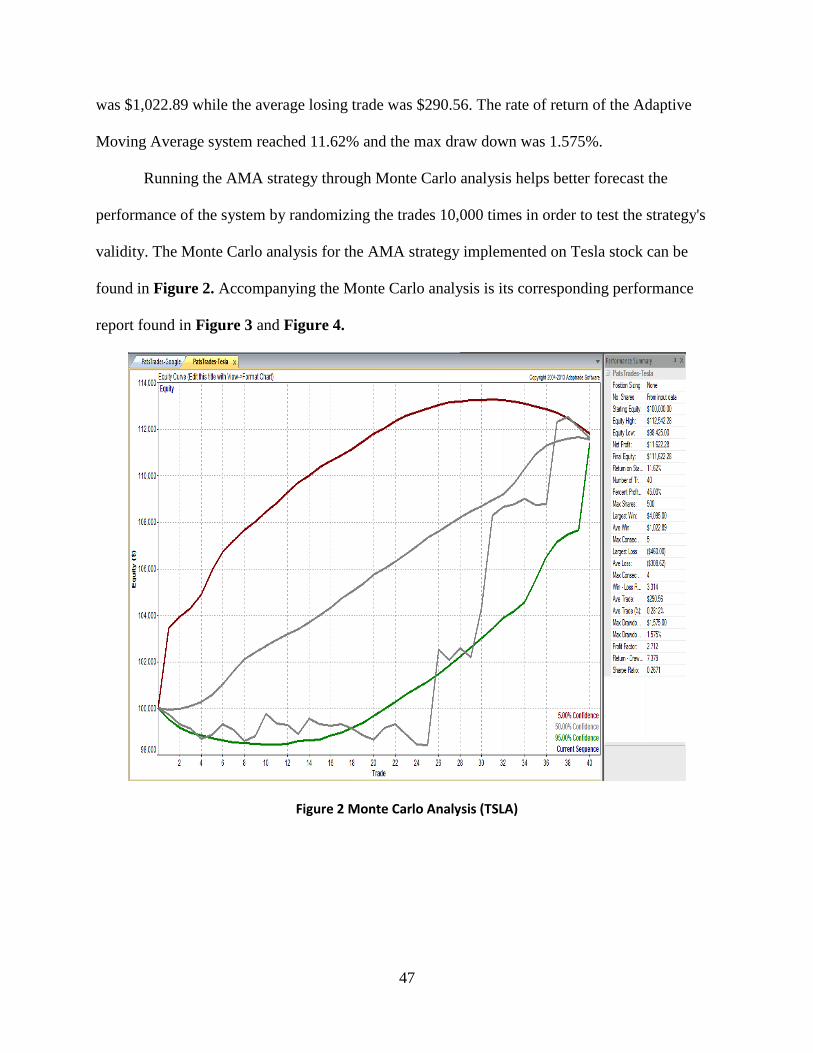
47
was $1,022.89 while the average losing trade was $290.56. The rate of return of the Adaptive
Moving Average system reached 11.62% and the max draw down was 1.575%.
Running the AMA strategy through Monte Carlo analysis helps better forecast the
performance of the system by randomizing the trades 10,000 times in order to test the strategy's
validity. The Monte Carlo analysis for the AMA strategy implemented on Tesla stock can be
found in Figure 2. Accompanying the Monte Carlo analysis is its corresponding performance
report found in Figure 3 and Figure 4.
Figure 2 Monte Carlo Analysis (TSLA)
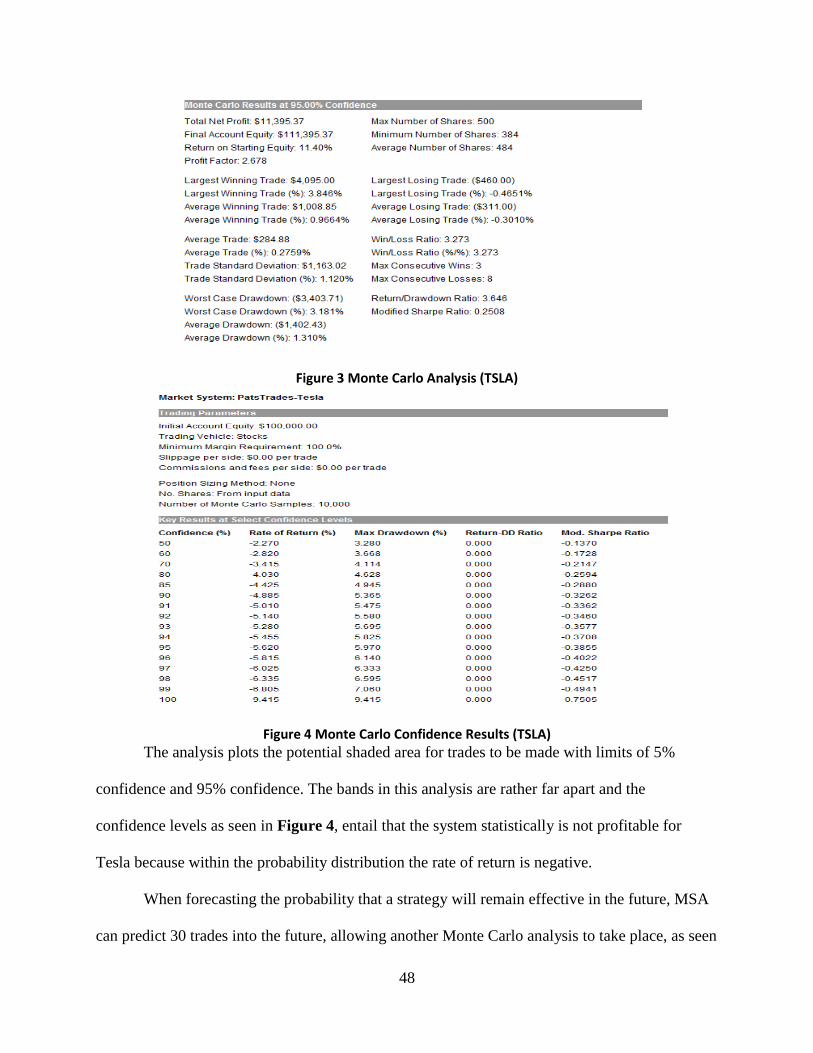
48
Figure 3 Monte Carlo Analysis (TSLA)
Figure 4 Monte Carlo Confidence Results (TSLA)
The analysis plots the potential shaded area for trades to be made with limits of 5%
confidence and 95% confidence. The bands in this analysis are rather far apart and the
confidence levels as seen in Figure 4, entail that the system statistically is not profitable for
Tesla because within the probability distribution the rate of return is negative.
When forecasting the probability that a strategy will remain effective in the future, MSA
can predict 30 trades into the future, allowing another Monte Carlo analysis to take place, as seen
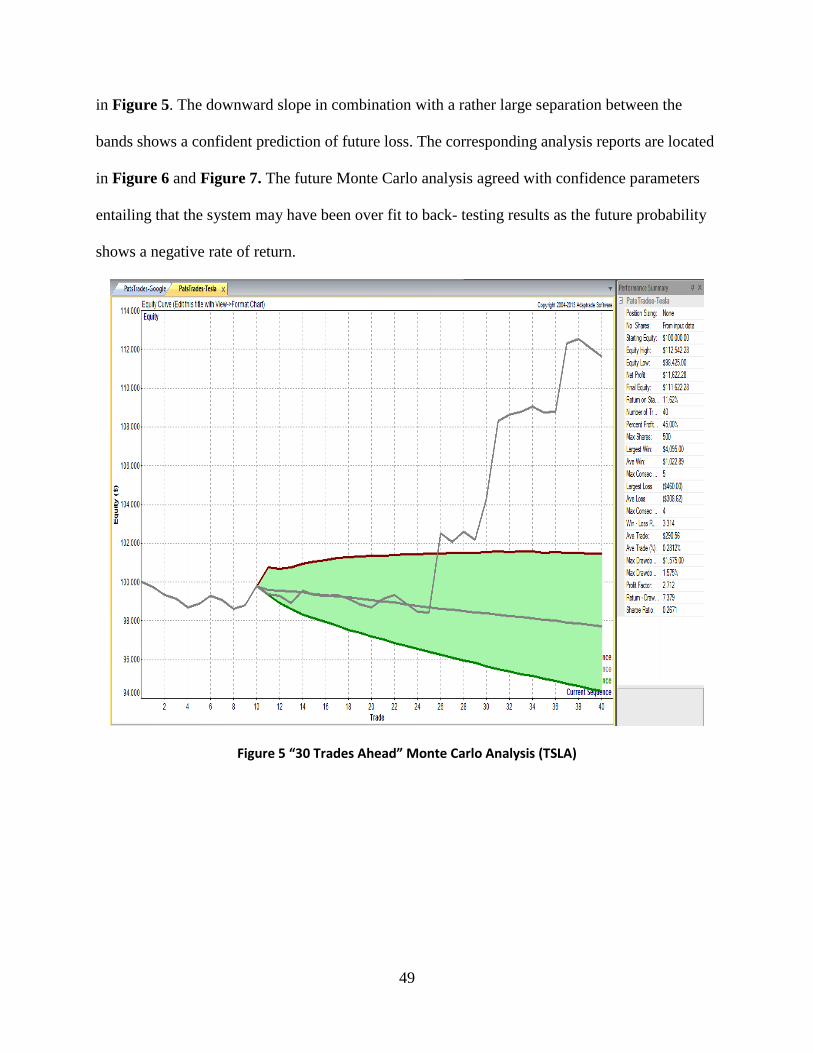
49
in Figure 5. The downward slope in combination with a rather large separation between the
bands shows a confident prediction of future loss. The corresponding analysis reports are located
in Figure 6 and Figure 7. The future Monte Carlo analysis agreed with confidence parameters
entailing that the system may have been over fit to back- testing results as the future probability
shows a negative rate of return.
Figure 5 “30 Trades Ahead” Monte Carlo Analysis (TSLA)
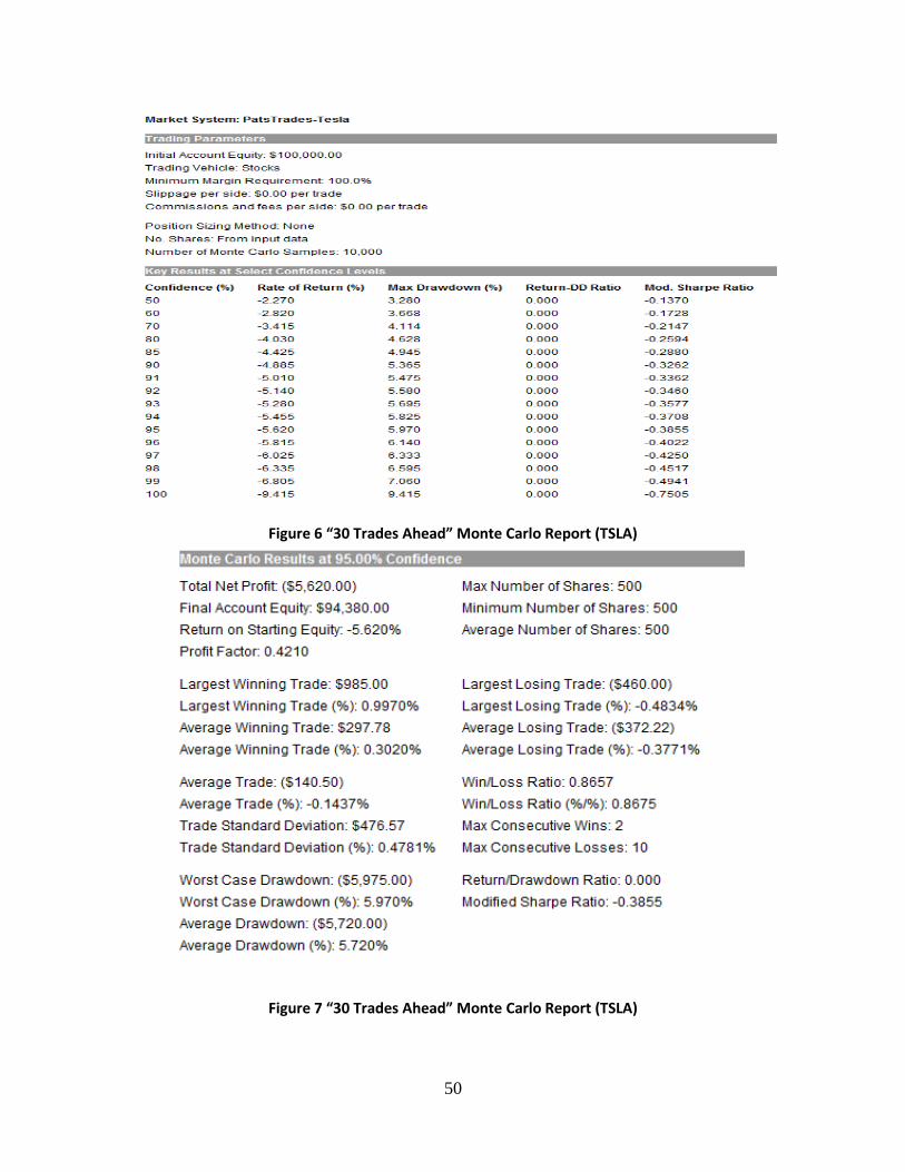
50
Figure 6 “30 Trades Ahead” Monte Carlo Report (TSLA)
Figure 7 “30 Trades Ahead” Monte Carlo Report (TSLA)
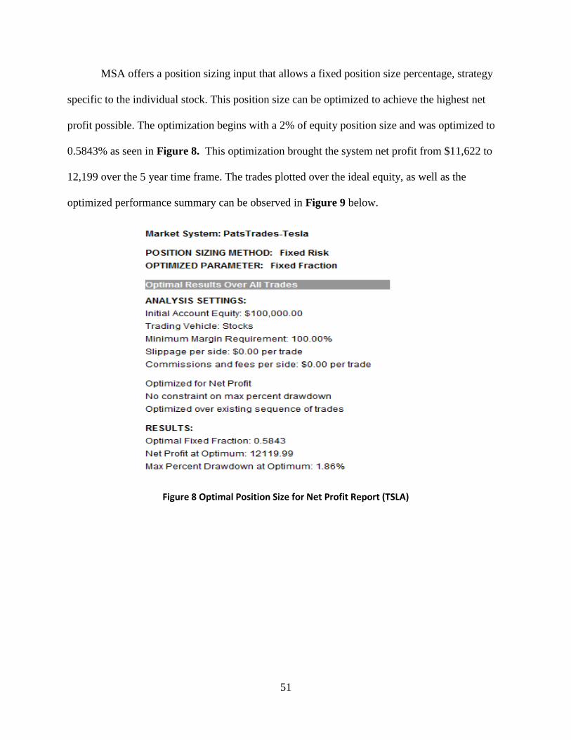
51
MSA offers a position sizing input that allows a fixed position size percentage, strategy
specific to the individual stock. This position size can be optimized to achieve the highest net
profit possible. The optimization begins with a 2% of equity position size and was optimized to
0.5843% as seen in Figure 8. This optimization brought the system net profit from $11,622 to
12,199 over the 5 year time frame. The trades plotted over the ideal equity, as well as the
optimized performance summary can be observed in Figure 9 below.
Figure 8 Optimal Position Size for Net Profit Report (TSLA)
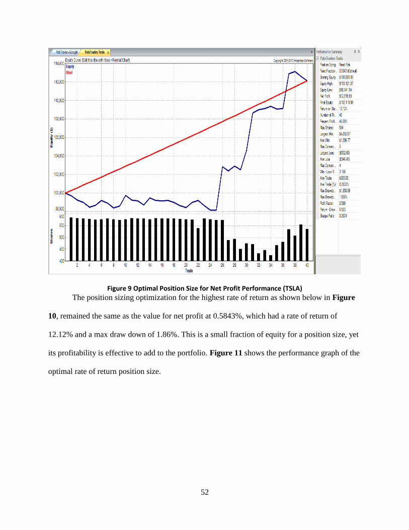
52
Figure 9 Optimal Position Size for Net Profit Performance (TSLA)
The position sizing optimization for the highest rate of return as shown below in Figure
10, remained the same as the value for net profit at 0.5843%, which had a rate of return of
12.12% and a max draw down of 1.86%. This is a small fraction of equity for a position size, yet
its profitability is effective to add to the portfolio. Figure 11 shows the performance graph of the
optimal rate of return position size.
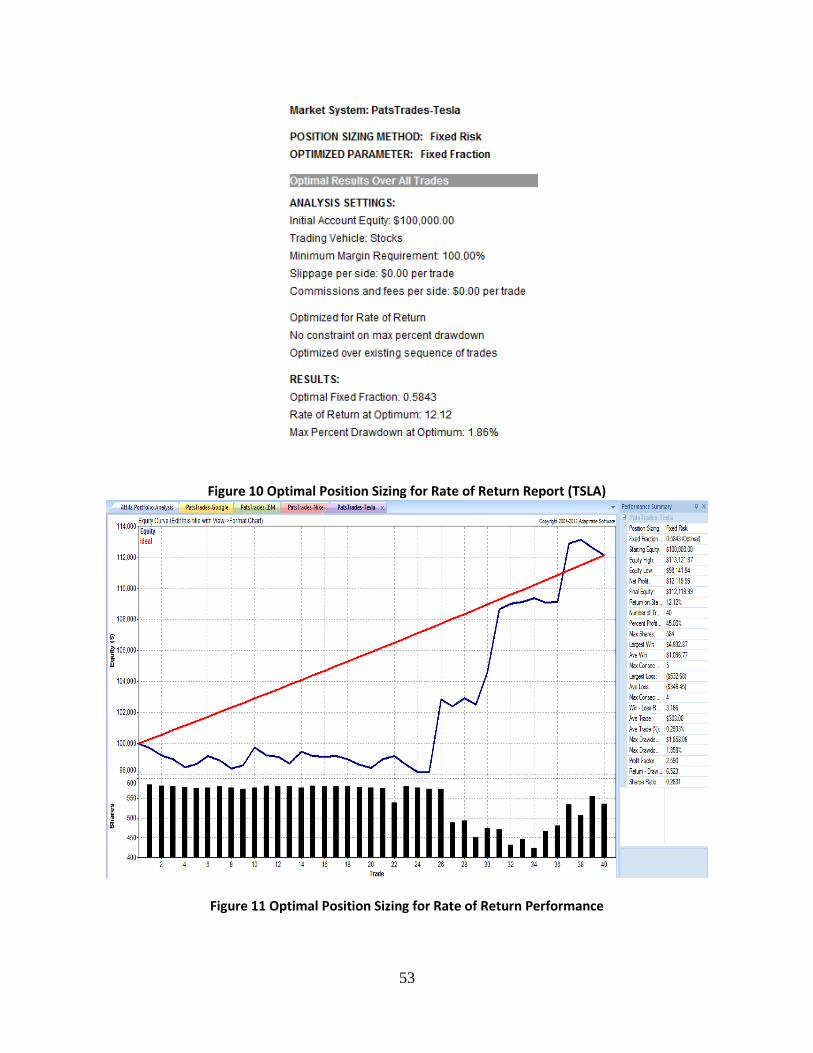
53
Figure 10 Optimal Position Sizing for Rate of Return Report (TSLA)
Figure 11 Optimal Position Sizing for Rate of Return Performance
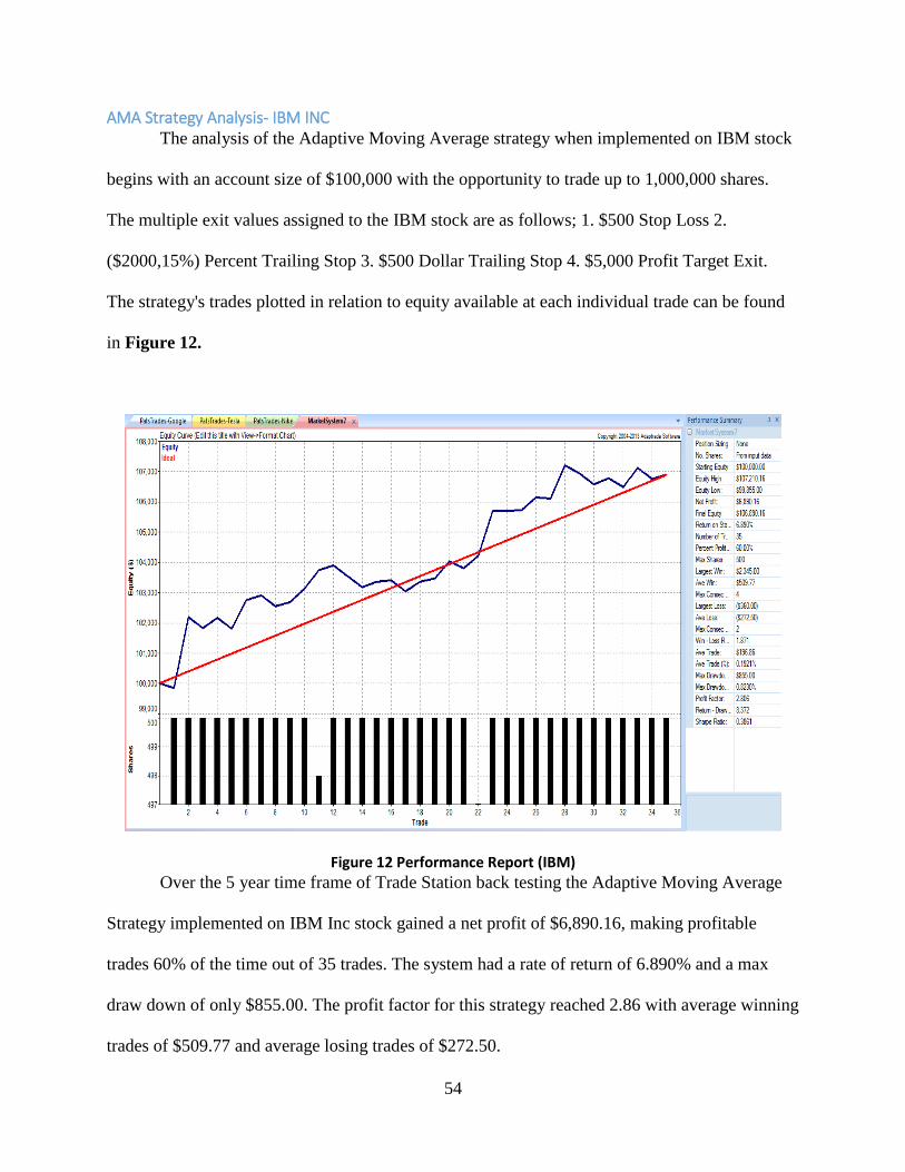
54
AMA Strategy Analysis- IBM INC The analysis of the Adaptive Moving Average strategy when implemented on IBM stock
begins with an account size of $100,000 with the opportunity to trade up to 1,000,000 shares.
The multiple exit values assigned to the IBM stock are as follows; 1. $500 Stop Loss 2.
($2000,15%) Percent Trailing Stop 3. $500 Dollar Trailing Stop 4. $5,000 Profit Target Exit.
The strategy's trades plotted in relation to equity available at each individual trade can be found
in Figure 12.
Figure 12 Performance Report (IBM)
Over the 5 year time frame of Trade Station back testing the Adaptive Moving Average
Strategy implemented on IBM Inc stock gained a net profit of $6,890.16, making profitable
trades 60% of the time out of 35 trades. The system had a rate of return of 6.890% and a max
draw down of only $855.00. The profit factor for this strategy reached 2.86 with average winning
trades of $509.77 and average losing trades of $272.50.
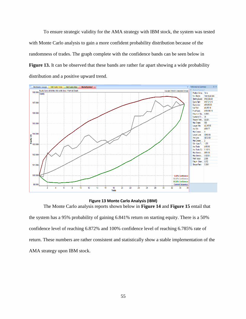
55
To ensure strategic validity for the AMA strategy with IBM stock, the system was tested
with Monte Carlo analysis to gain a more confident probability distribution because of the
randomness of trades. The graph complete with the confidence bands can be seen below in
Figure 13. It can be observed that these bands are rather far apart showing a wide probability
distribution and a positive upward trend.
Figure 13 Monte Carlo Analysis (IBM)
The Monte Carlo analysis reports shown below in Figure 14 and Figure 15 entail that
the system has a 95% probability of gaining 6.841% return on starting equity. There is a 50%
confidence level of reaching 6.872% and 100% confidence level of reaching 6.785% rate of
return. These numbers are rather consistent and statistically show a stable implementation of the
AMA strategy upon IBM stock.
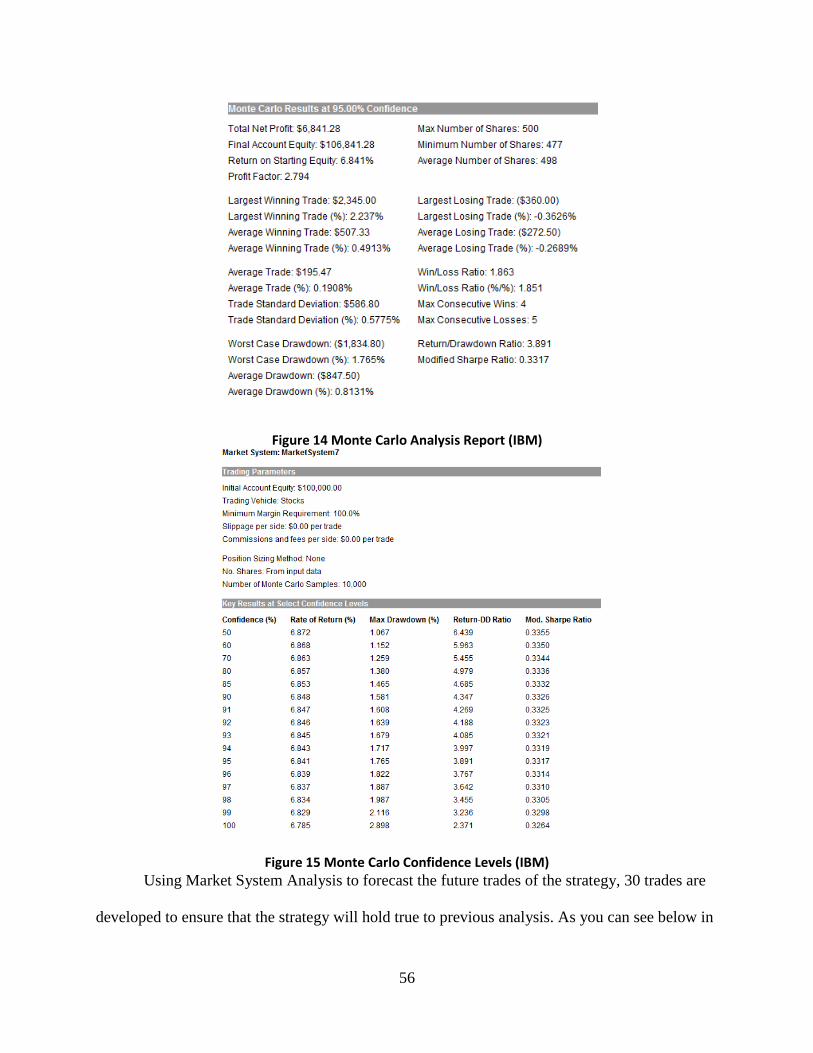
56
Figure 14 Monte Carlo Analysis Report (IBM)
Figure 15 Monte Carlo Confidence Levels (IBM)
Using Market System Analysis to forecast the future trades of the strategy, 30 trades are
developed to ensure that the strategy will hold true to previous analysis. As you can see below in
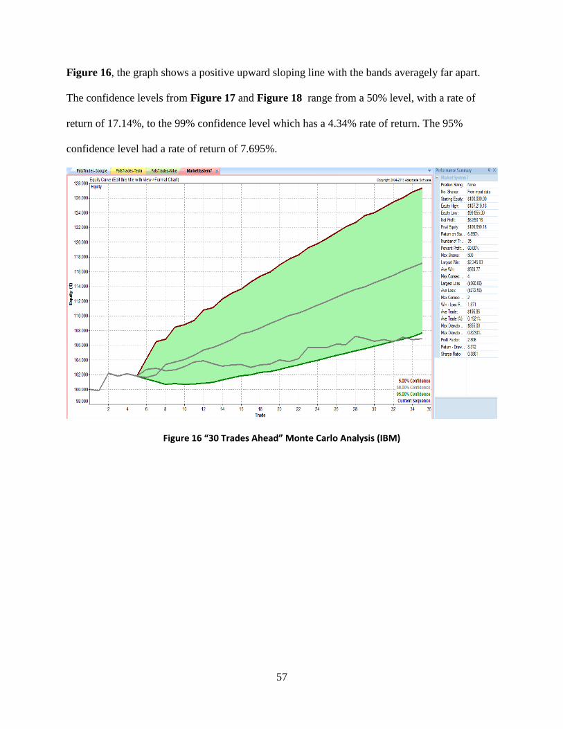
57
Figure 16, the graph shows a positive upward sloping line with the bands averagely far apart.
The confidence levels from Figure 17 and Figure 18 range from a 50% level, with a rate of
return of 17.14%, to the 99% confidence level which has a 4.34% rate of return. The 95%
confidence level had a rate of return of 7.695%.
Figure 16 “30 Trades Ahead” Monte Carlo Analysis (IBM)
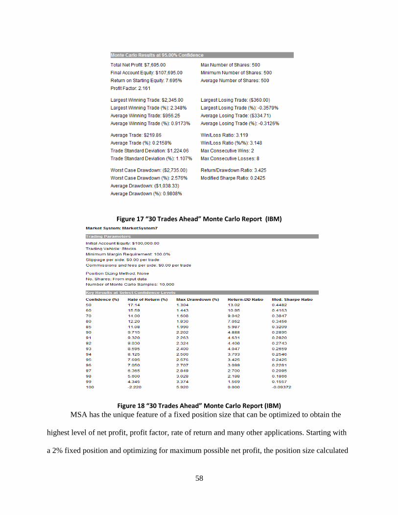
58
Figure 17 “30 Trades Ahead” Monte Carlo Report (IBM)
Figure 18 “30 Trades Ahead” Monte Carlo Report (IBM)
MSA has the unique feature of a fixed position size that can be optimized to obtain the
highest level of net profit, profit factor, rate of return and many other applications. Starting with
a 2% fixed position and optimizing for maximum possible net profit, the position size calculated
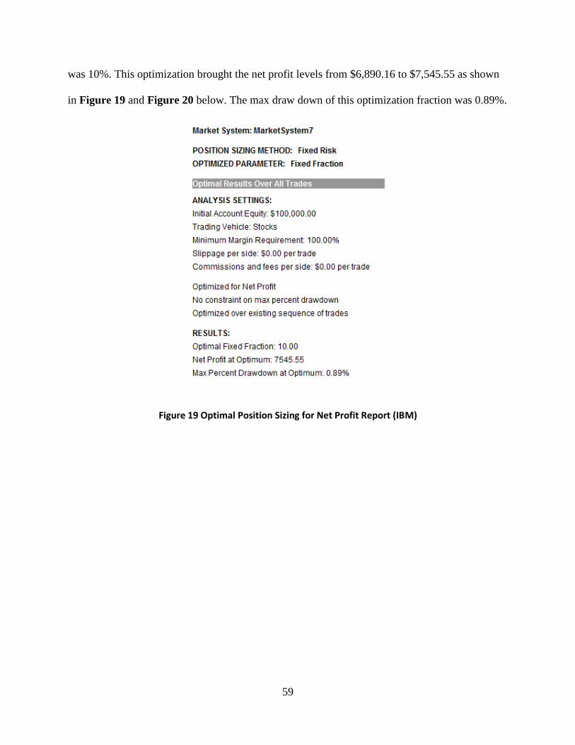
59
was 10%. This optimization brought the net profit levels from $6,890.16 to $7,545.55 as shown
in Figure 19 and Figure 20 below. The max draw down of this optimization fraction was 0.89%.
Figure 19 Optimal Position Sizing for Net Profit Report (IBM)
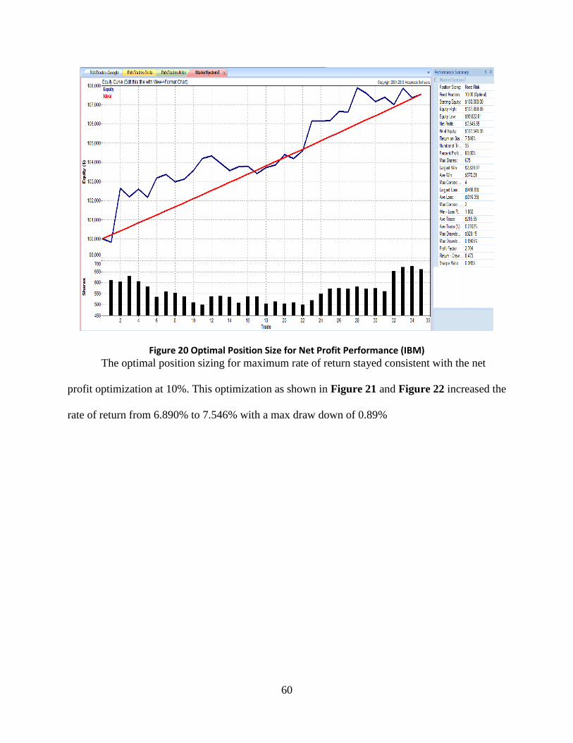
60
Figure 20 Optimal Position Size for Net Profit Performance (IBM)
The optimal position sizing for maximum rate of return stayed consistent with the net
profit optimization at 10%. This optimization as shown in Figure 21 and Figure 22 increased the
rate of return from 6.890% to 7.546% with a max draw down of 0.89%
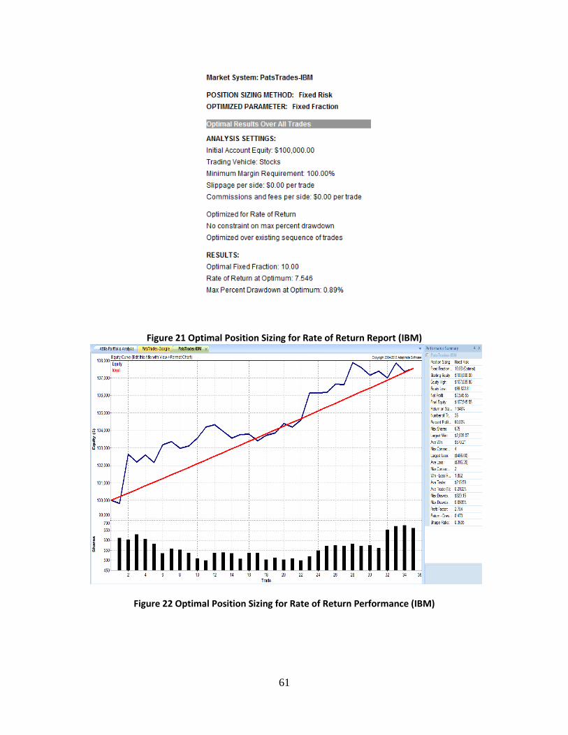
61
Figure 21 Optimal Position Sizing for Rate of Return Report (IBM)
Figure 22 Optimal Position Sizing for Rate of Return Performance (IBM)
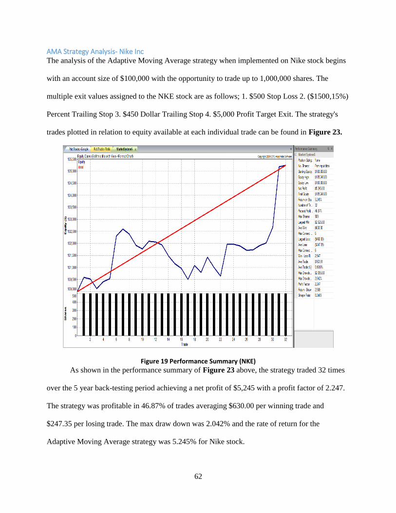
62
AMA Strategy Analysis- Nike Inc The analysis of the Adaptive Moving Average strategy when implemented on Nike stock begins
with an account size of $100,000 with the opportunity to trade up to 1,000,000 shares. The
multiple exit values assigned to the NKE stock are as follows; 1. $500 Stop Loss 2. ($1500,15%)
Percent Trailing Stop 3. $450 Dollar Trailing Stop 4. $5,000 Profit Target Exit. The strategy's
trades plotted in relation to equity available at each individual trade can be found in Figure 23.
Figure 19 Performance Summary (NKE)
As shown in the performance summary of Figure 23 above, the strategy traded 32 times
over the 5 year back-testing period achieving a net profit of $5,245 with a profit factor of 2.247.
The strategy was profitable in 46.87% of trades averaging $630.00 per winning trade and
$247.35 per losing trade. The max draw down was 2.042% and the rate of return for the
Adaptive Moving Average strategy was 5.245% for Nike stock.
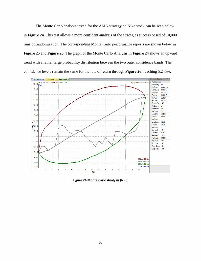
63
The Monte Carlo analysis tested for the AMA strategy on Nike stock can be seen below
in Figure 24. This test allows a more confident analysis of the strategies success based of 10,000
runs of randomization. The corresponding Monte Carlo performance reports are shown below in
Figure 25 and Figure 26. The graph of the Monte Carlo Analysis in Figure 24 shows an upward
trend with a rather large probability distribution between the two outer confidence bands. The
confidence levels remain the same for the rate of return through Figure 26, reaching 5.245%.
Figure 24 Monte Carlo Analysis (NKE)
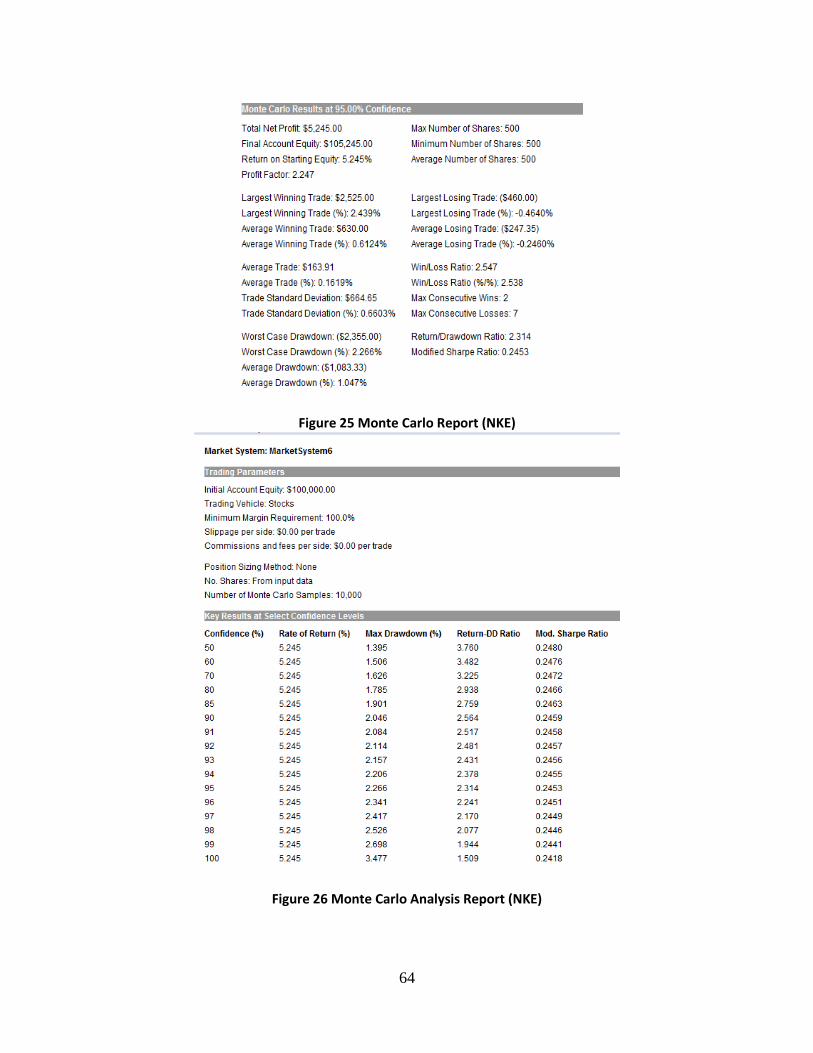
64
Figure 25 Monte Carlo Report (NKE)
Figure 26 Monte Carlo Analysis Report (NKE)
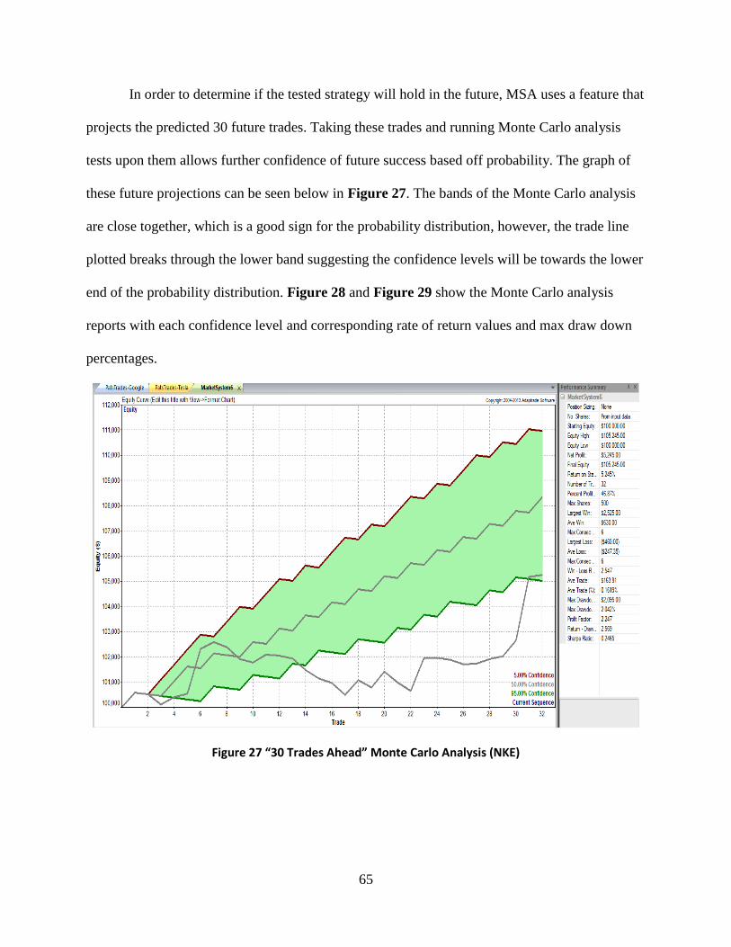
65
In order to determine if the tested strategy will hold in the future, MSA uses a feature that
projects the predicted 30 future trades. Taking these trades and running Monte Carlo analysis
tests upon them allows further confidence of future success based off probability. The graph of
these future projections can be seen below in Figure 27. The bands of the Monte Carlo analysis
are close together, which is a good sign for the probability distribution, however, the trade line
plotted breaks through the lower band suggesting the confidence levels will be towards the lower
end of the probability distribution. Figure 28 and Figure 29 show the Monte Carlo analysis
reports with each confidence level and corresponding rate of return values and max draw down
percentages.
Figure 27 “30 Trades Ahead” Monte Carlo Analysis (NKE)
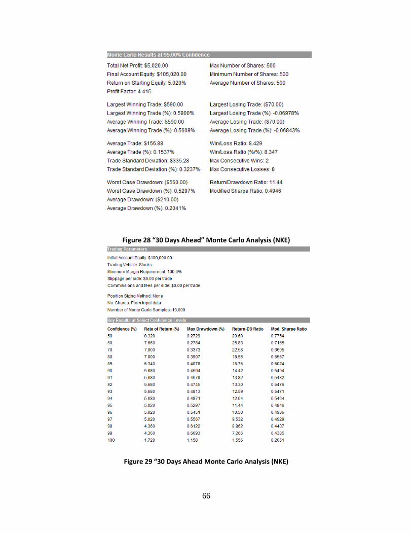
66
Figure 28 “30 Days Ahead” Monte Carlo Analysis (NKE)
Figure 29 “30 Days Ahead Monte Carlo Analysis (NKE)
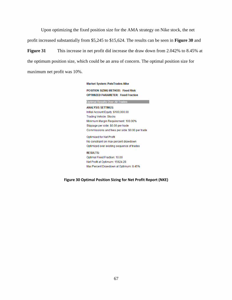
67
Upon optimizing the fixed position size for the AMA strategy on Nike stock, the net
profit increased substantially from $5,245 to $15,624. The results can be seen in Figure 30 and
Figure 31 This increase in net profit did increase the draw down from 2.042% to 8.45% at
the optimum position size, which could be an area of concern. The optimal position size for
maximum net profit was 10%.
Figure 30 Optimal Position Sizing for Net Profit Report (NKE)
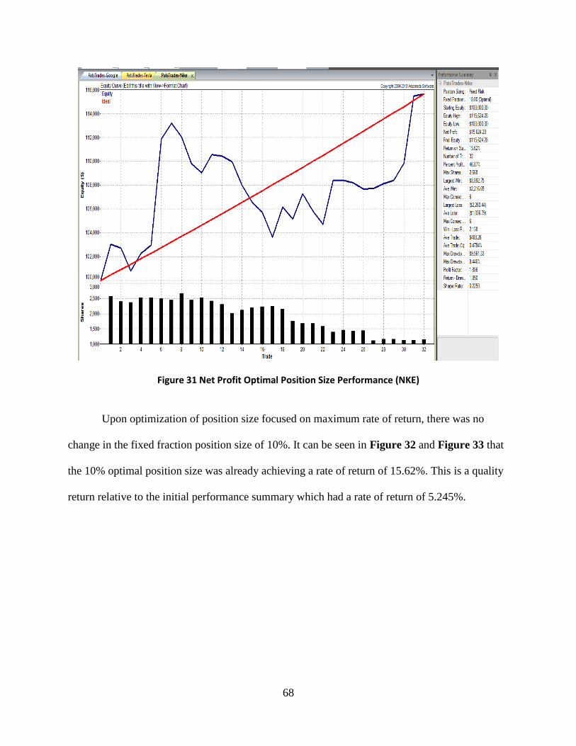
68
Figure 31 Net Profit Optimal Position Size Performance (NKE)
Upon optimization of position size focused on maximum rate of return, there was no
change in the fixed fraction position size of 10%. It can be seen in Figure 32 and Figure 33 that
the 10% optimal position size was already achieving a rate of return of 15.62%. This is a quality
return relative to the initial performance summary which had a rate of return of 5.245%.
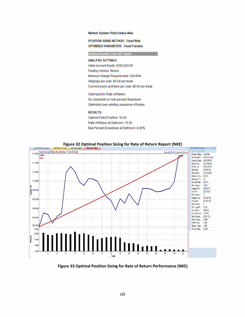
69
Figure 32 Optimal Position Sizing for Rate of Return Report (NKE)
Figure 33 Optimal Position Sizing for Rate of Return Performance (NKE)
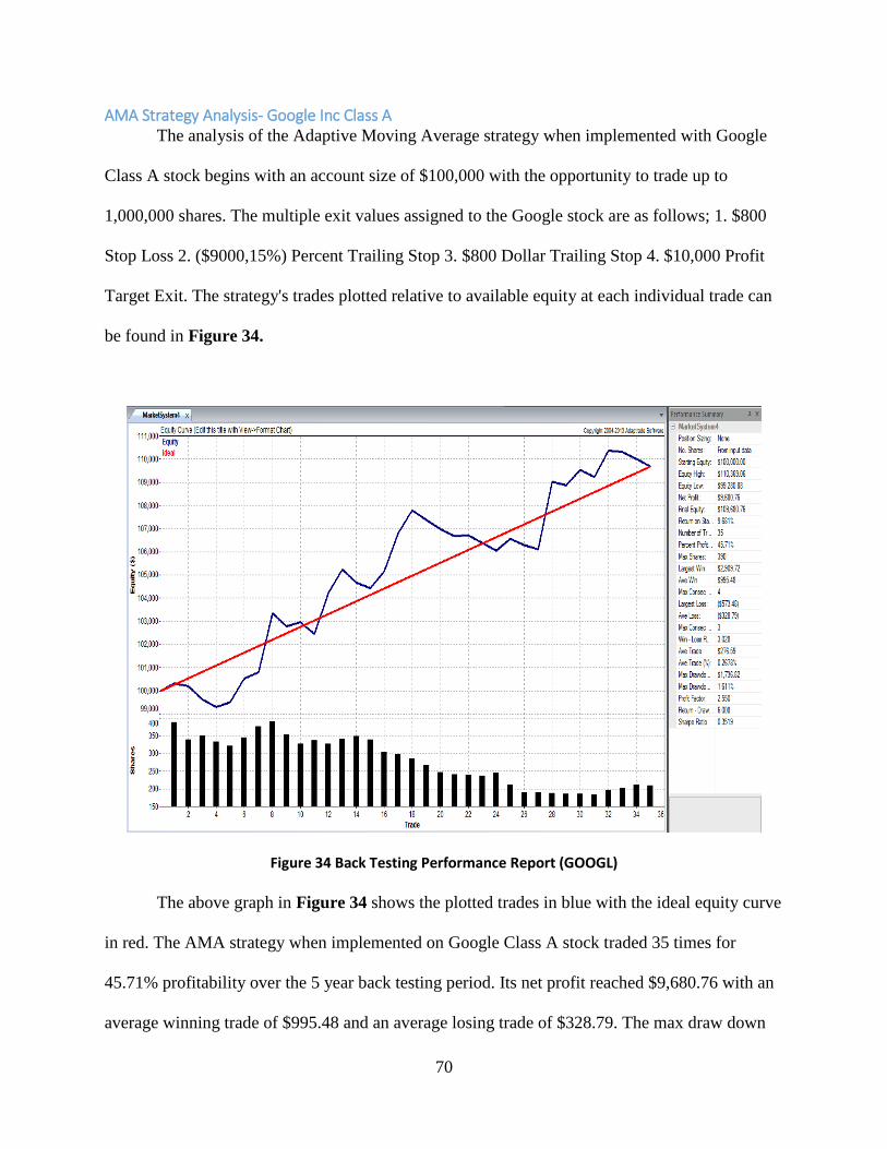
70
AMA Strategy Analysis- Google Inc Class A The analysis of the Adaptive Moving Average strategy when implemented with Google
Class A stock begins with an account size of $100,000 with the opportunity to trade up to
1,000,000 shares. The multiple exit values assigned to the Google stock are as follows; 1. $800
Stop Loss 2. ($9000,15%) Percent Trailing Stop 3. $800 Dollar Trailing Stop 4. $10,000 Profit
Target Exit. The strategy's trades plotted relative to available equity at each individual trade can
be found in Figure 34.
Figure 34 Back Testing Performance Report (GOOGL)
The above graph in Figure 34 shows the plotted trades in blue with the ideal equity curve
in red. The AMA strategy when implemented on Google Class A stock traded 35 times for
45.71% profitability over the 5 year back testing period. Its net profit reached $9,680.76 with an
average winning trade of $995.48 and an average losing trade of $328.79. The max draw down
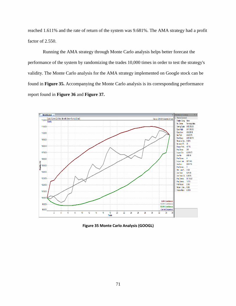
71
reached 1.611% and the rate of return of the system was 9.681%. The AMA strategy had a profit
factor of 2.550.
Running the AMA strategy through Monte Carlo analysis helps better forecast the
performance of the system by randomizing the trades 10,000 times in order to test the strategy's
validity. The Monte Carlo analysis for the AMA strategy implemented on Google stock can be
found in Figure 35. Accompanying the Monte Carlo analysis is its corresponding performance
report found in Figure 36 and Figure 37.
Figure 35 Monte Carlo Analysis (GOOGL)
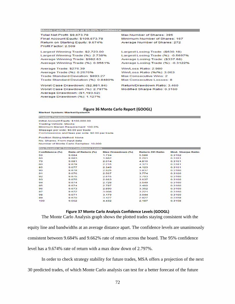
72
Figure 36 Monte Carlo Report (GOOGL)
Figure 37 Monte Carlo Analysis Confidence Levels (GOOGL)
The Monte Carlo Analysis graph shows the plotted trades staying consistent with the
equity line and bandwidths at an average distance apart. The confidence levels are unanimously
consistent between 9.684% and 9.662% rate of return across the board. The 95% confidence
level has a 9.674% rate of return with a max draw down of 2.797%.
In order to check strategy stability for future trades, MSA offers a projection of the next
30 predicted trades, of which Monte Carlo analysis can test for a better forecast of the future
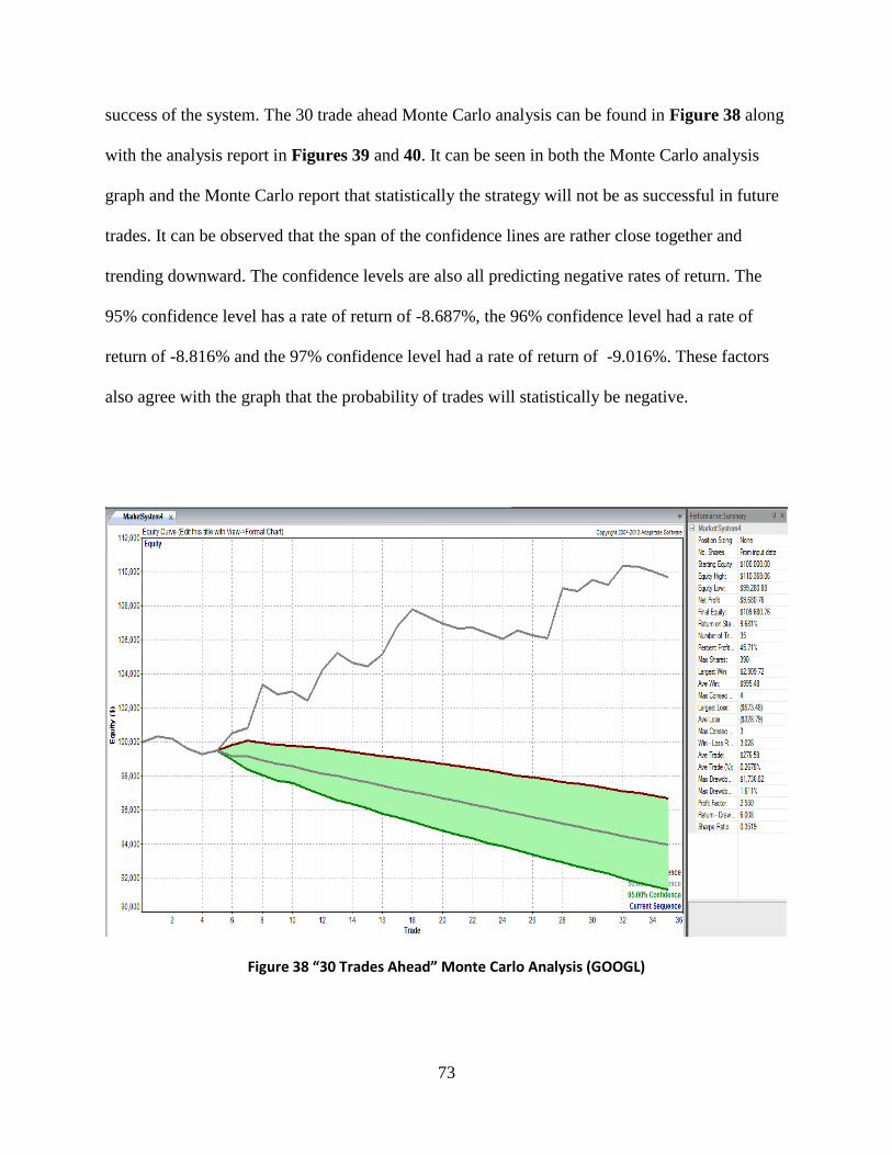
73
success of the system. The 30 trade ahead Monte Carlo analysis can be found in Figure 38 along
with the analysis report in Figures 39 and 40. It can be seen in both the Monte Carlo analysis
graph and the Monte Carlo report that statistically the strategy will not be as successful in future
trades. It can be observed that the span of the confidence lines are rather close together and
trending downward. The confidence levels are also all predicting negative rates of return. The
95% confidence level has a rate of return of -8.687%, the 96% confidence level had a rate of
return of -8.816% and the 97% confidence level had a rate of return of -9.016%. These factors
also agree with the graph that the probability of trades will statistically be negative.
Figure 38 “30 Trades Ahead” Monte Carlo Analysis (GOOGL)
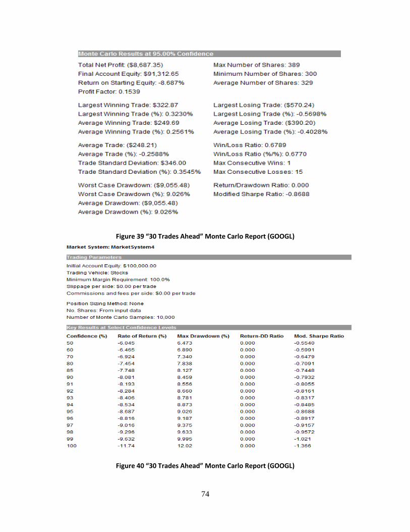
74
Figure 39 “30 Trades Ahead” Monte Carlo Report (GOOGL)
Figure 40 “30 Trades Ahead” Monte Carlo Report (GOOGL)
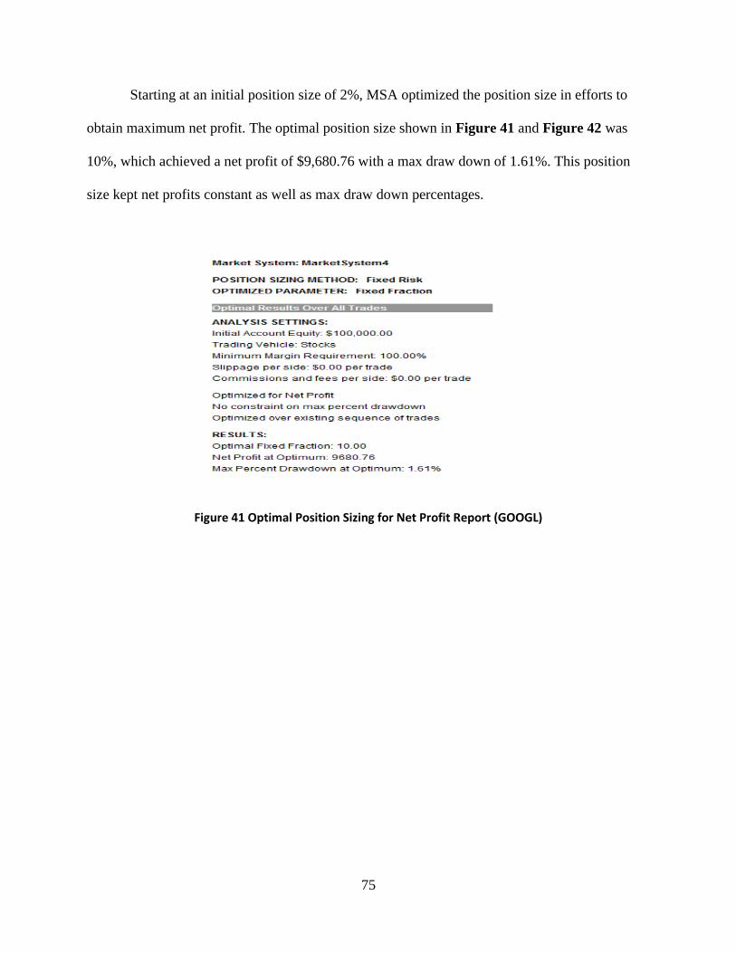
75
Starting at an initial position size of 2%, MSA optimized the position size in efforts to
obtain maximum net profit. The optimal position size shown in Figure 41 and Figure 42 was
10%, which achieved a net profit of $9,680.76 with a max draw down of 1.61%. This position
size kept net profits constant as well as max draw down percentages.
Figure 41 Optimal Position Sizing for Net Profit Report (GOOGL)
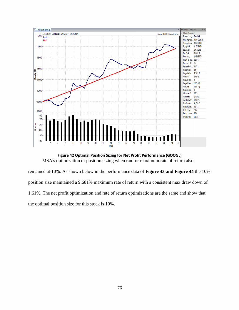
76
Figure 42 Optimal Position Sizing for Net Profit Performance (GOOGL)
MSA's optimization of position sizing when ran for maximum rate of return also
remained at 10%. As shown below in the performance data of Figure 43 and Figure 44 the 10%
position size maintained a 9.681% maximum rate of return with a consistent max draw down of
1.61%. The net profit optimization and rate of return optimizations are the same and show that
the optimal position size for this stock is 10%.
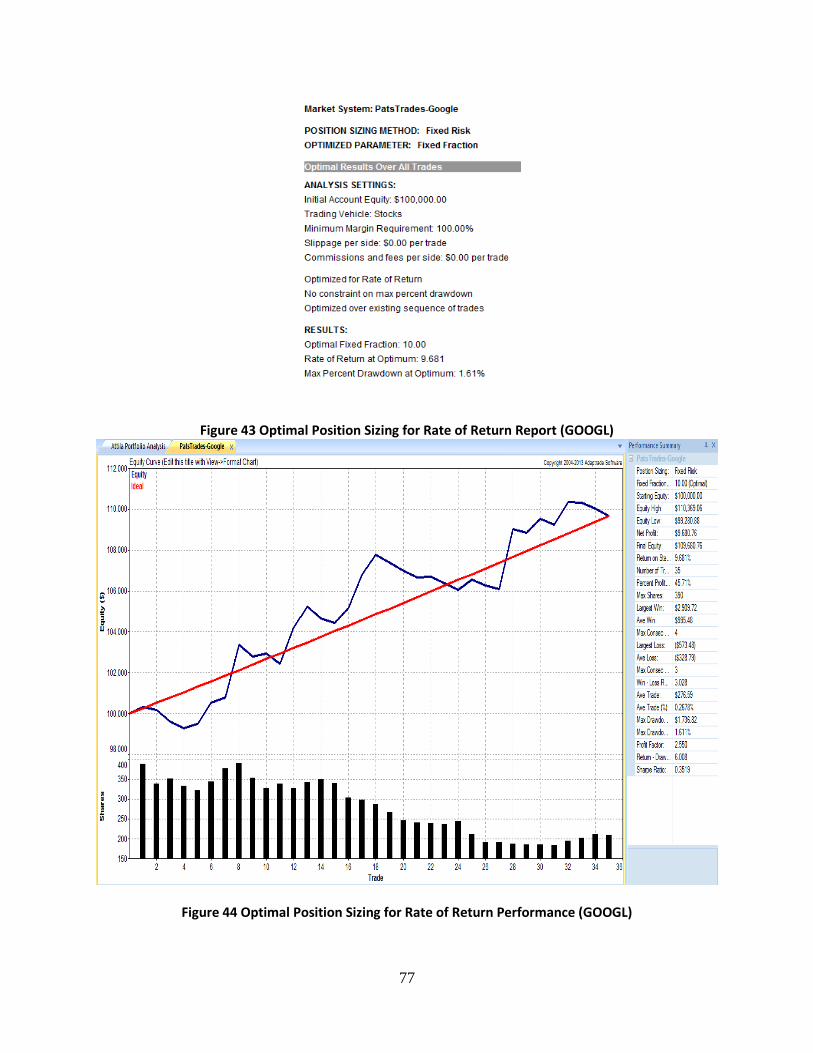
77
Figure 43 Optimal Position Sizing for Rate of Return Report (GOOGL)
Figure 44 Optimal Position Sizing for Rate of Return Performance (GOOGL)
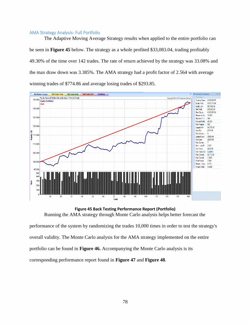
78
AMA Strategy Analysis- Full Portfolio The Adaptive Moving Average Strategy results when applied to the entire portfolio can
be seen in Figure 45 below. The strategy as a whole profited $33,083.04, trading profitably
49.30% of the time over 142 trades. The rate of return achieved by the strategy was 33.08% and
the max draw down was 3.385%. The AMA strategy had a profit factor of 2.564 with average
winning trades of $774.86 and average losing trades of $293.85.
Figure 45 Back Testing Performance Report (Portfolio)
Running the AMA strategy through Monte Carlo analysis helps better forecast the
performance of the system by randomizing the trades 10,000 times in order to test the strategy's
overall validity. The Monte Carlo analysis for the AMA strategy implemented on the entire
portfolio can be found in Figure 46. Accompanying the Monte Carlo analysis is its
corresponding performance report found in Figure 47 and Figure 48.
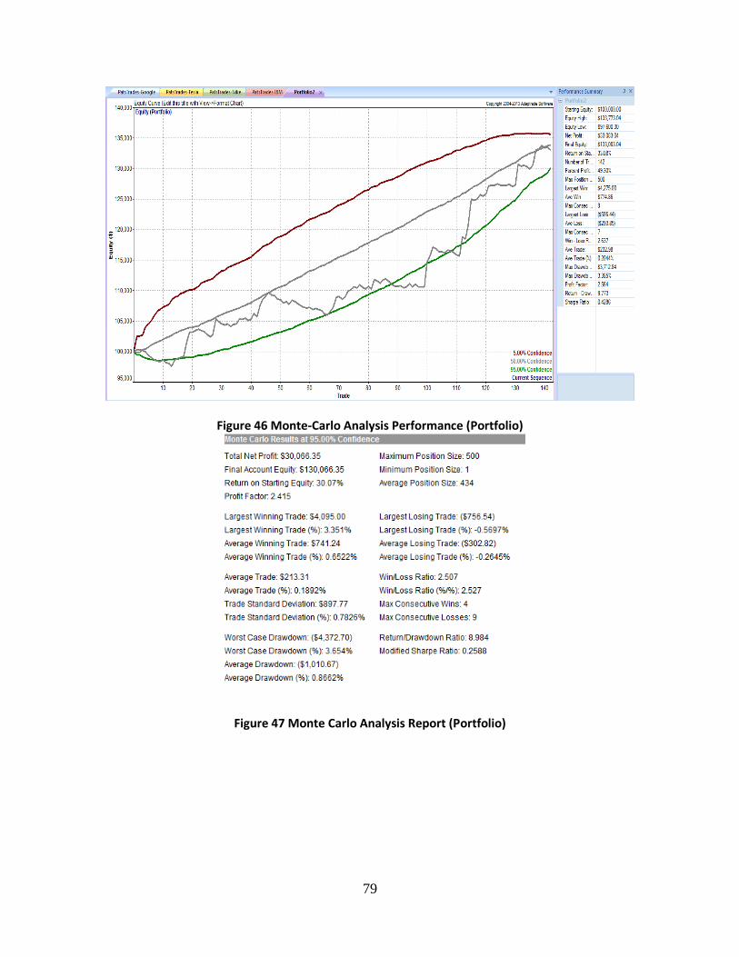
79
Figure 46 Monte-Carlo Analysis Performance (Portfolio)
Figure 47 Monte Carlo Analysis Report (Portfolio)
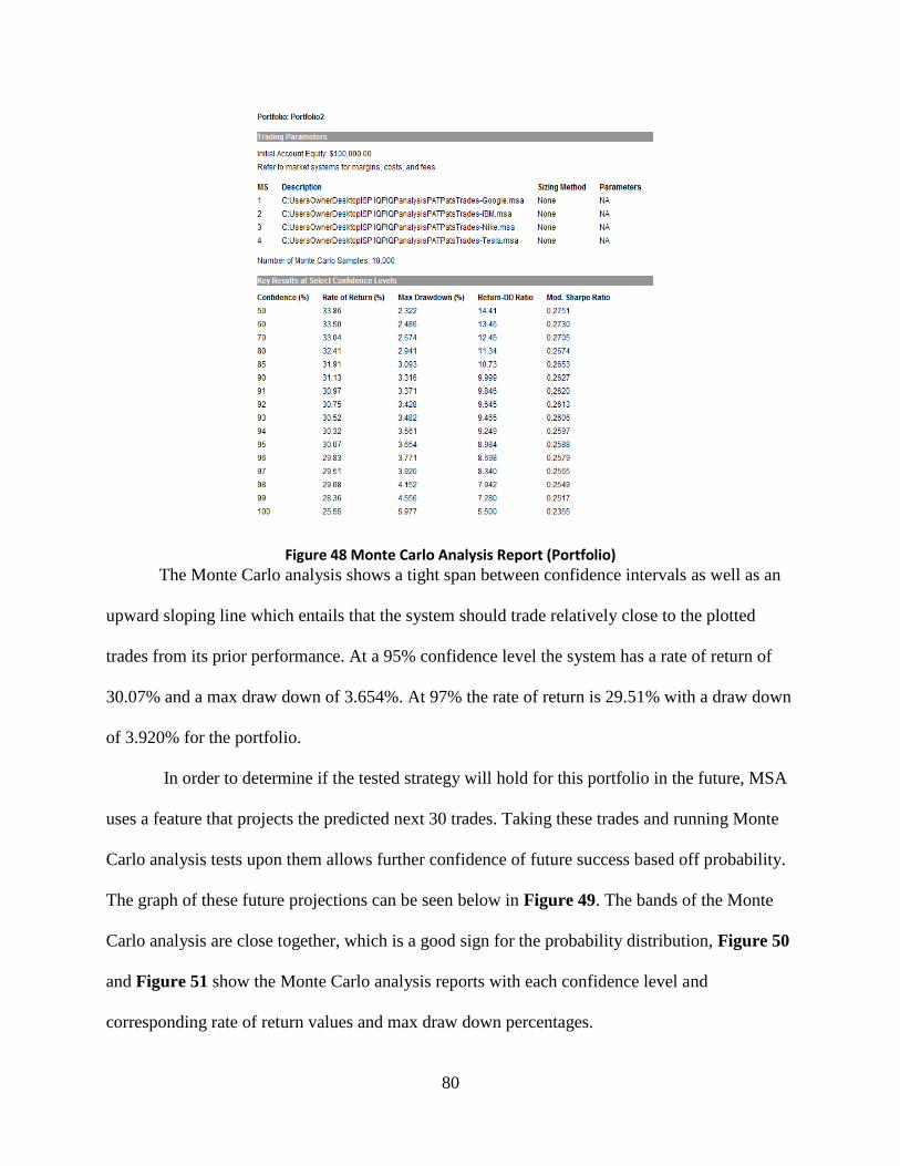
80
Figure 48 Monte Carlo Analysis Report (Portfolio)
The Monte Carlo analysis shows a tight span between confidence intervals as well as an
upward sloping line which entails that the system should trade relatively close to the plotted
trades from its prior performance. At a 95% confidence level the system has a rate of return of
30.07% and a max draw down of 3.654%. At 97% the rate of return is 29.51% with a draw down
of 3.920% for the portfolio.
In order to determine if the tested strategy will hold for this portfolio in the future, MSA
uses a feature that projects the predicted next 30 trades. Taking these trades and running Monte
Carlo analysis tests upon them allows further confidence of future success based off probability.
The graph of these future projections can be seen below in Figure 49. The bands of the Monte
Carlo analysis are close together, which is a good sign for the probability distribution, Figure 50
and Figure 51 show the Monte Carlo analysis reports with each confidence level and
corresponding rate of return values and max draw down percentages.
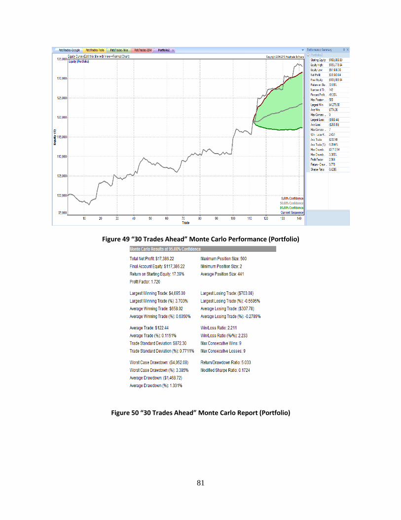
81
Figure 49 “30 Trades Ahead” Monte Carlo Performance (Portfolio)
Figure 50 “30 Trades Ahead” Monte Carlo Report (Portfolio)
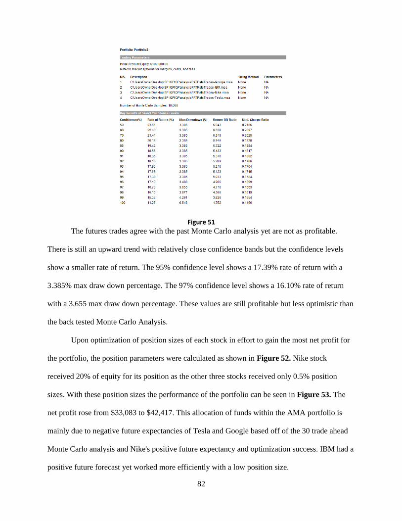
82
Figure 51
The futures trades agree with the past Monte Carlo analysis yet are not as profitable.
There is still an upward trend with relatively close confidence bands but the confidence levels
show a smaller rate of return. The 95% confidence level shows a 17.39% rate of return with a
3.385% max draw down percentage. The 97% confidence level shows a 16.10% rate of return
with a 3.655 max draw down percentage. These values are still profitable but less optimistic than
the back tested Monte Carlo Analysis.
Upon optimization of position sizes of each stock in effort to gain the most net profit for
the portfolio, the position parameters were calculated as shown in Figure 52. Nike stock
received 20% of equity for its position as the other three stocks received only 0.5% position
sizes. With these position sizes the performance of the portfolio can be seen in Figure 53. The
net profit rose from $33,083 to $42,417. This allocation of funds within the AMA portfolio is
mainly due to negative future expectancies of Tesla and Google based off of the 30 trade ahead
Monte Carlo analysis and Nike's positive future expectancy and optimization success. IBM had a
positive future forecast yet worked more efficiently with a low position size.
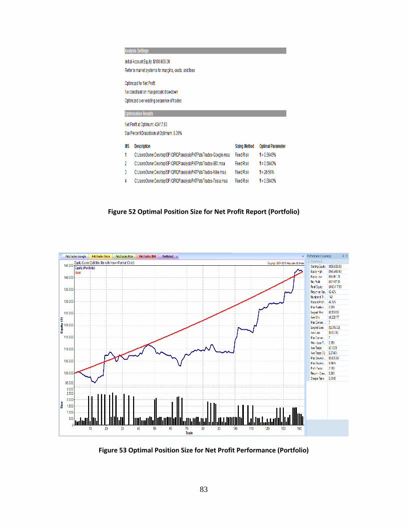
83
Figure 52 Optimal Position Size for Net Profit Report (Portfolio)
Figure 53 Optimal Position Size for Net Profit Performance (Portfolio)
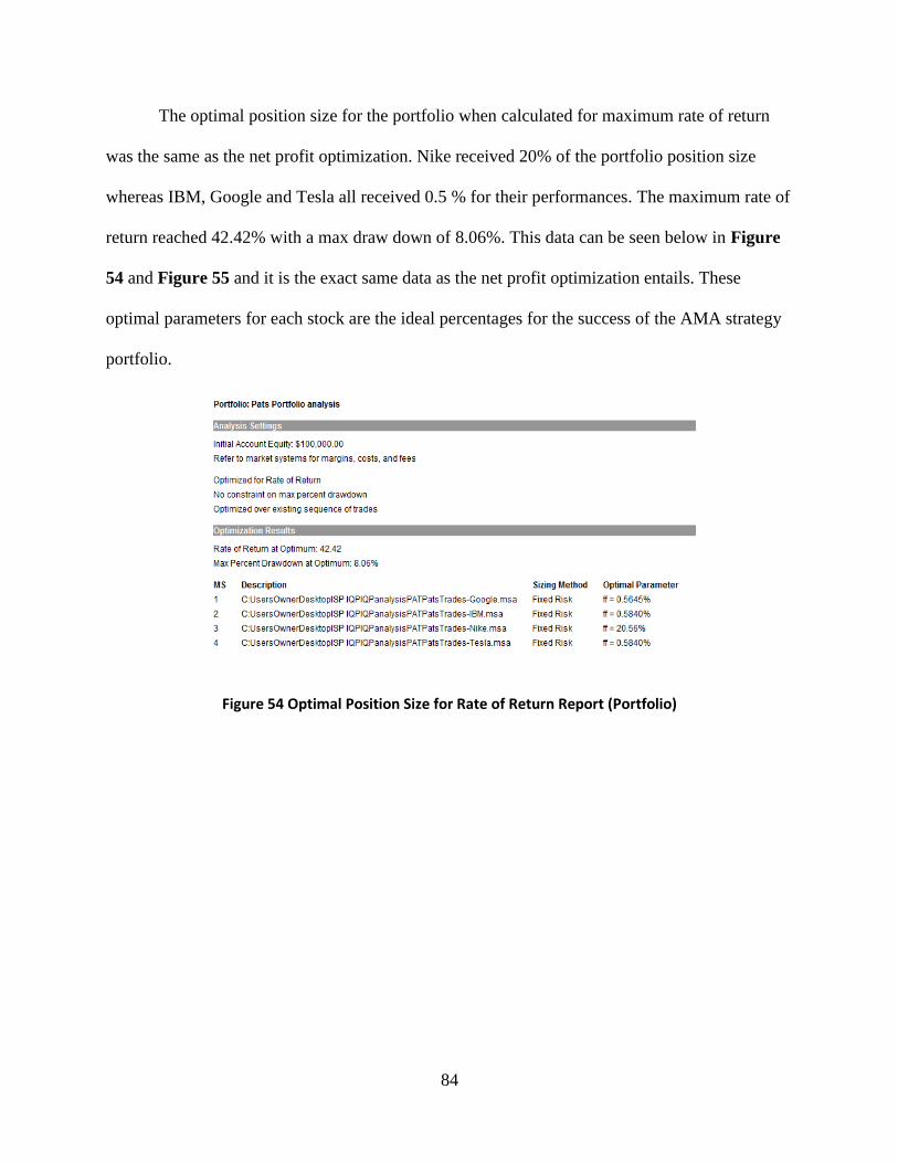
84
The optimal position size for the portfolio when calculated for maximum rate of return
was the same as the net profit optimization. Nike received 20% of the portfolio position size
whereas IBM, Google and Tesla all received 0.5 % for their performances. The maximum rate of
return reached 42.42% with a max draw down of 8.06%. This data can be seen below in Figure
54 and Figure 55 and it is the exact same data as the net profit optimization entails. These
optimal parameters for each stock are the ideal percentages for the success of the AMA strategy
portfolio.
Figure 54 Optimal Position Size for Rate of Return Report (Portfolio)
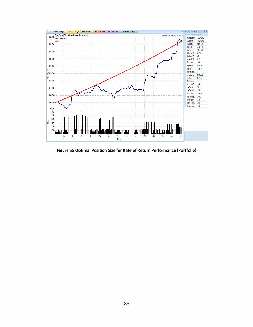
85
Figure 55 Optimal Position Size for Rate of Return Performance (Portfolio)
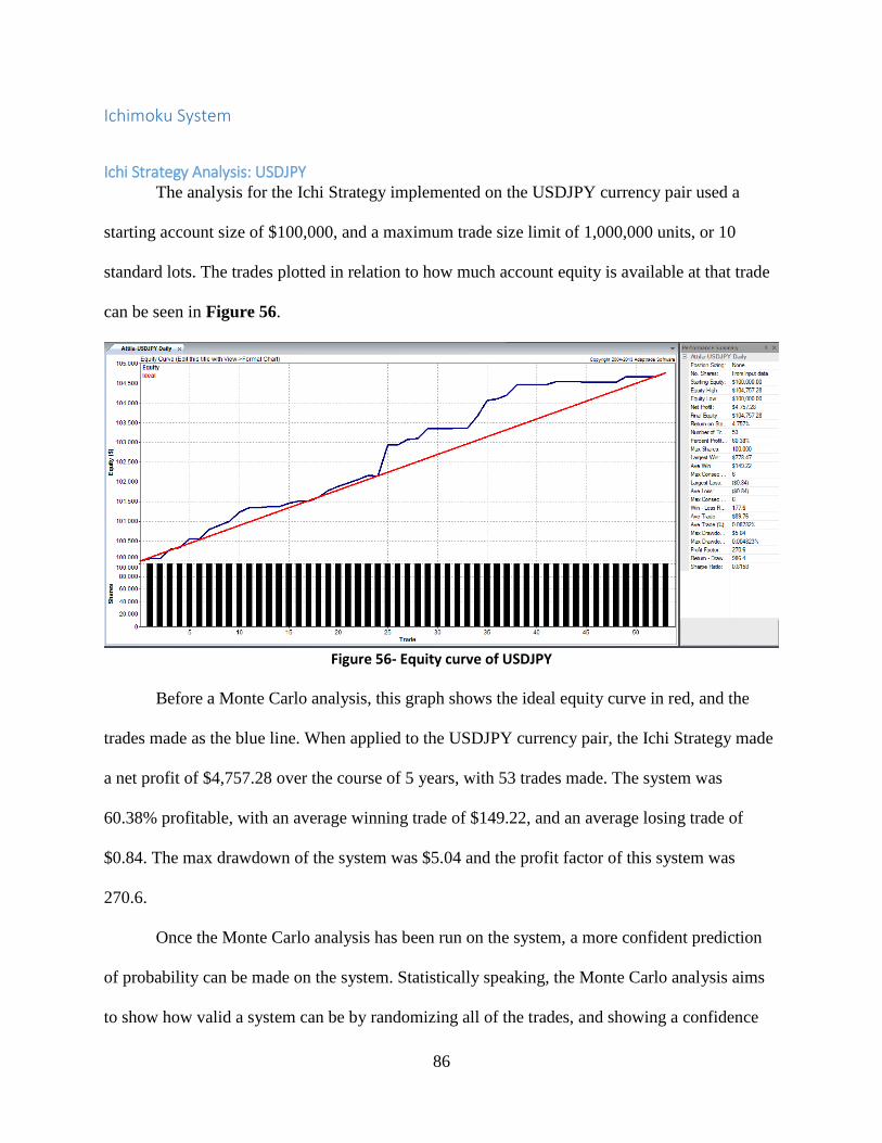
86
Ichimoku System
Ichi Strategy Analysis: USDJPY The analysis for the Ichi Strategy implemented on the USDJPY currency pair used a
starting account size of $100,000, and a maximum trade size limit of 1,000,000 units, or 10
standard lots. The trades plotted in relation to how much account equity is available at that trade
can be seen in Figure 56.
Figure 56- Equity curve of USDJPY
Before a Monte Carlo analysis, this graph shows the ideal equity curve in red, and the
trades made as the blue line. When applied to the USDJPY currency pair, the Ichi Strategy made
a net profit of $4,757.28 over the course of 5 years, with 53 trades made. The system was
60.38% profitable, with an average winning trade of $149.22, and an average losing trade of
$0.84. The max drawdown of the system was $5.04 and the profit factor of this system was
270.6.
Once the Monte Carlo analysis has been run on the system, a more confident prediction
of probability can be made on the system. Statistically speaking, the Monte Carlo analysis aims
to show how valid a system can be by randomizing all of the trades, and showing a confidence
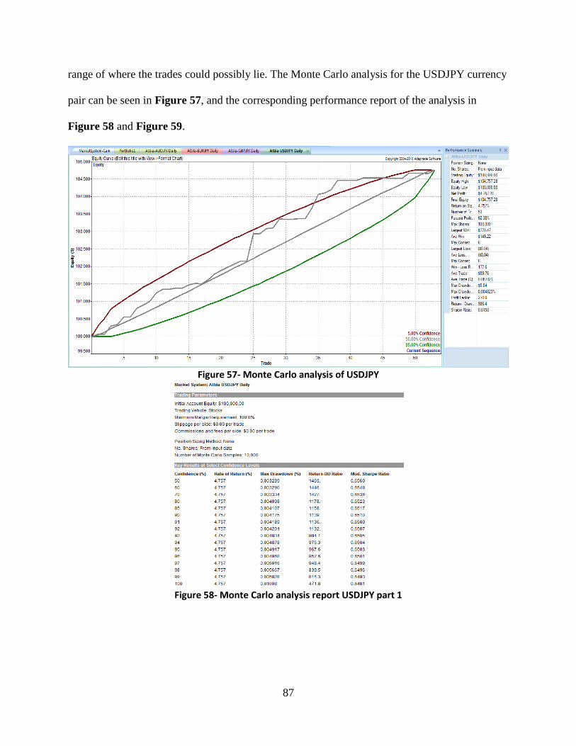
87
range of where the trades could possibly lie. The Monte Carlo analysis for the USDJPY currency
pair can be seen in Figure 57, and the corresponding performance report of the analysis in
Figure 58 and Figure 59.
Figure 57- Monte Carlo analysis of USDJPY
Figure 58- Monte Carlo analysis report USDJPY part 1
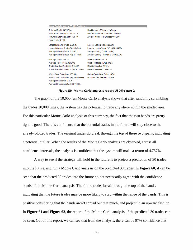
88
Figure 59- Monte Carlo analysis report USDJPY part 2
The graph of the 10,000 run Monte Carlo analysis shows that after randomly scrambling
the trades 10,000 times, the system has the potential to trade anywhere within the shaded area.
For this particular Monte Carlo analysis of this currency, the fact that the two bands are pretty
tight is good. There is confidence that the potential trades in the future will stay close to the
already plotted trades. The original trades do break through the top of these two spans, indicating
a potential outlier. When the results of the Monte Carlo analysis are observed, across all
confidence intervals, the analysis is confident that the system will make a return of 4.757%.
A way to see if the strategy will hold in the future is to project a prediction of 30 trades
into the future, and run a Monte Carlo analysis on the predicted 30 trades. In Figure 60, it can be
seen that the predicted 30 trades into the future do not necessarily agree with the confidence
bands of the Monte Carlo analysis. The future trades break through the top of the bands,
indicating that the future trades may be more likely to stay within the range of the bands. This is
positive considering that the bands aren’t spread out that much, and project in an upward fashion.
In Figure 61 and Figure 62, the report of the Monte Carlo analysis of the predicted 30 trades can
be seen. Out of this report, we can see that from the analysis, there can be 97% confidence that
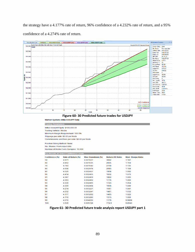
89
the strategy have a 4.177% rate of return, 96% confidence of a 4.232% rate of return, and a 95%
confidence of a 4.274% rate of return.
Figure 60- 30 Predicted future trades for USDJPY
Figure 61- 30 Predicted future trade analysis report USDJPY part 1
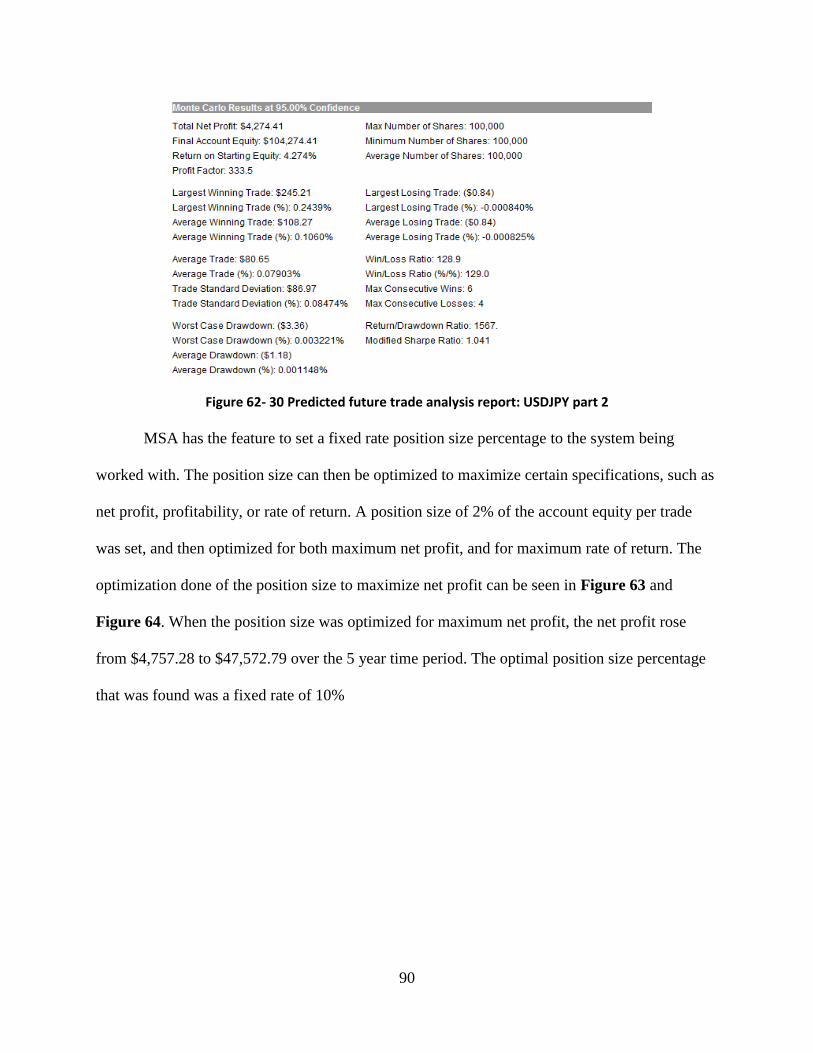
90
Figure 62- 30 Predicted future trade analysis report: USDJPY part 2
MSA has the feature to set a fixed rate position size percentage to the system being
worked with. The position size can then be optimized to maximize certain specifications, such as
net profit, profitability, or rate of return. A position size of 2% of the account equity per trade
was set, and then optimized for both maximum net profit, and for maximum rate of return. The
optimization done of the position size to maximize net profit can be seen in Figure 63 and
Figure 64. When the position size was optimized for maximum net profit, the net profit rose
from $4,757.28 to $47,572.79 over the 5 year time period. The optimal position size percentage
that was found was a fixed rate of 10%
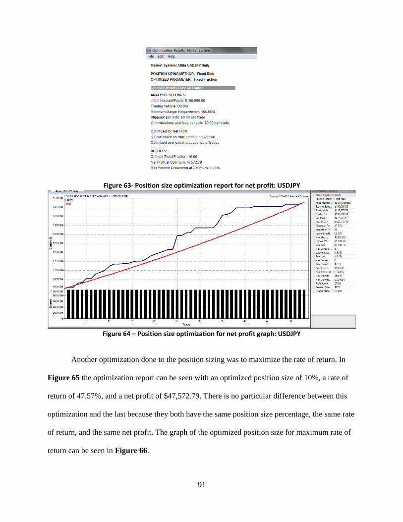
91
Figure 63- Position size optimization report for net profit: USDJPY
Figure 64 – Position size optimization for net profit graph: USDJPY
Another optimization done to the position sizing was to maximize the rate of return. In
Figure 65 the optimization report can be seen with an optimized position size of 10%, a rate of
return of 47.57%, and a net profit of $47,572.79. There is no particular difference between this
optimization and the last because they both have the same position size percentage, the same rate
of return, and the same net profit. The graph of the optimized position size for maximum rate of
return can be seen in Figure 66.
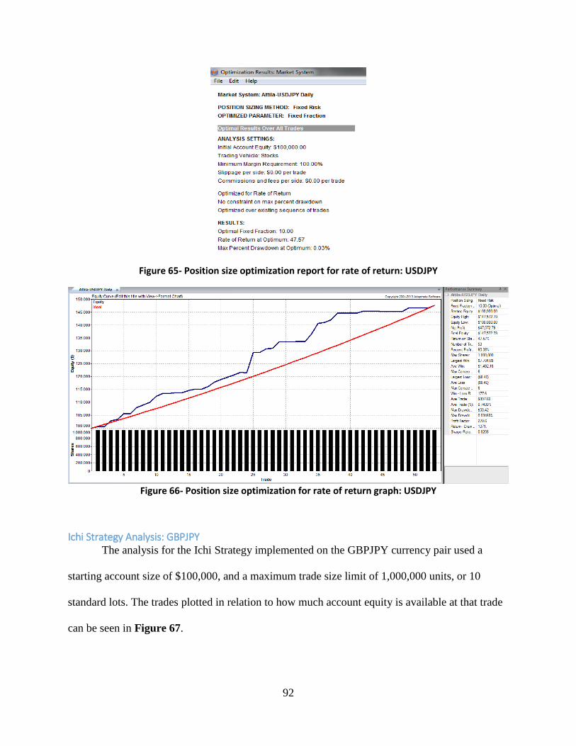
92
Figure 65- Position size optimization report for rate of return: USDJPY
Figure 66- Position size optimization for rate of return graph: USDJPY
Ichi Strategy Analysis: GBPJPY The analysis for the Ichi Strategy implemented on the GBPJPY currency pair used a
starting account size of $100,000, and a maximum trade size limit of 1,000,000 units, or 10
standard lots. The trades plotted in relation to how much account equity is available at that trade
can be seen in Figure 67.
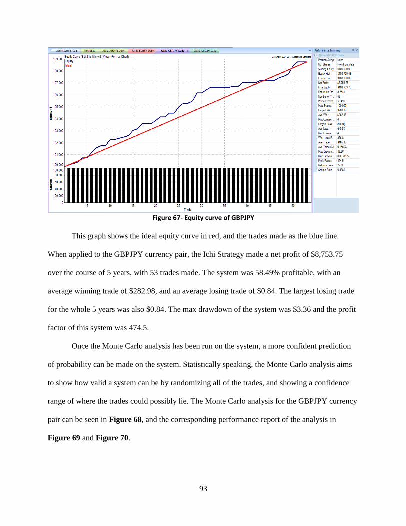
93
Figure 67- Equity curve of GBPJPY
This graph shows the ideal equity curve in red, and the trades made as the blue line.
When applied to the GBPJPY currency pair, the Ichi Strategy made a net profit of $8,753.75
over the course of 5 years, with 53 trades made. The system was 58.49% profitable, with an
average winning trade of $282.98, and an average losing trade of $0.84. The largest losing trade
for the whole 5 years was also $0.84. The max drawdown of the system was $3.36 and the profit
factor of this system was 474.5.
Once the Monte Carlo analysis has been run on the system, a more confident prediction
of probability can be made on the system. Statistically speaking, the Monte Carlo analysis aims
to show how valid a system can be by randomizing all of the trades, and showing a confidence
range of where the trades could possibly lie. The Monte Carlo analysis for the GBPJPY currency
pair can be seen in Figure 68, and the corresponding performance report of the analysis in
Figure 69 and Figure 70.
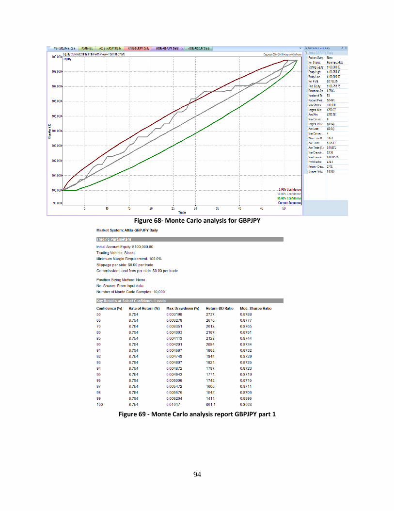
94
Figure 68- Monte Carlo analysis for GBPJPY
Figure 69 - Monte Carlo analysis report GBPJPY part 1
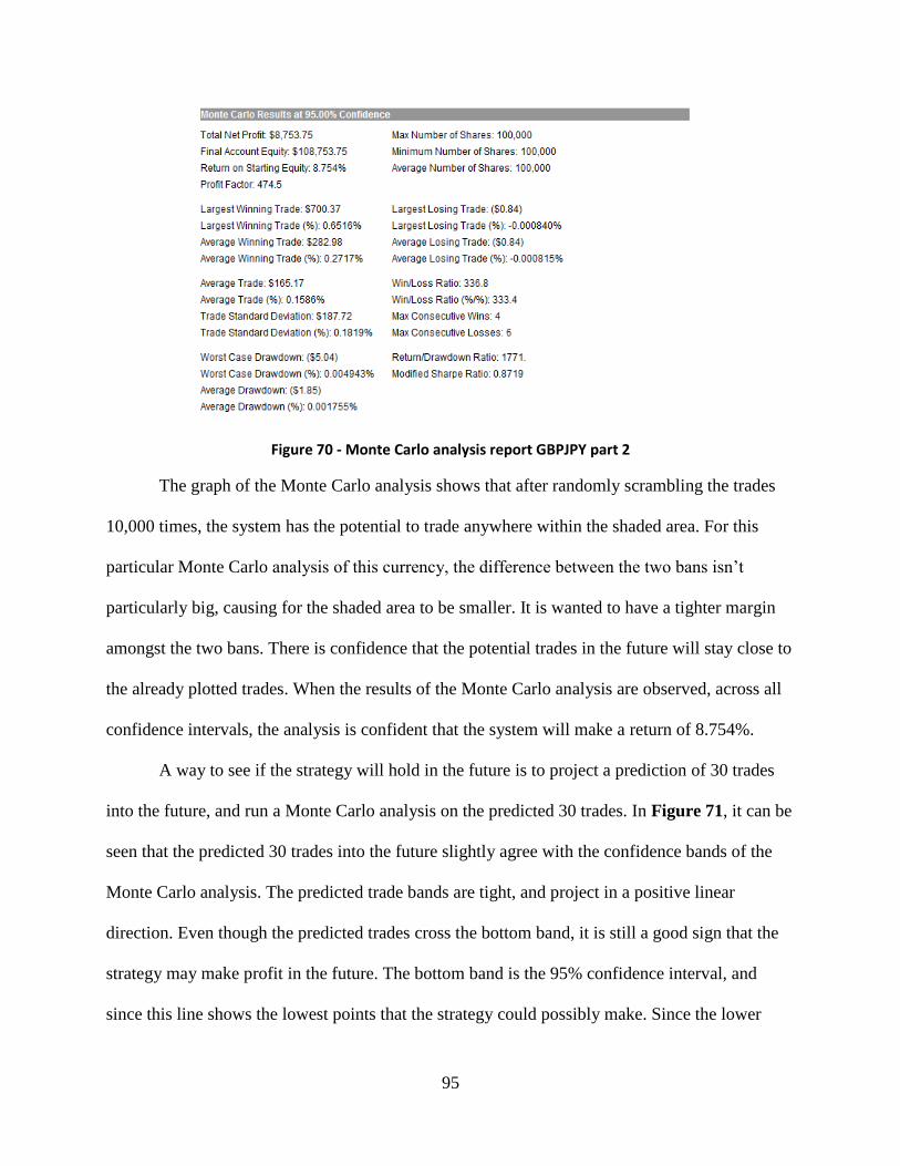
95
Figure 70 - Monte Carlo analysis report GBPJPY part 2
The graph of the Monte Carlo analysis shows that after randomly scrambling the trades
10,000 times, the system has the potential to trade anywhere within the shaded area. For this
particular Monte Carlo analysis of this currency, the difference between the two bans isn’t
particularly big, causing for the shaded area to be smaller. It is wanted to have a tighter margin
amongst the two bans. There is confidence that the potential trades in the future will stay close to
the already plotted trades. When the results of the Monte Carlo analysis are observed, across all
confidence intervals, the analysis is confident that the system will make a return of 8.754%.
A way to see if the strategy will hold in the future is to project a prediction of 30 trades
into the future, and run a Monte Carlo analysis on the predicted 30 trades. In Figure 71, it can be
seen that the predicted 30 trades into the future slightly agree with the confidence bands of the
Monte Carlo analysis. The predicted trade bands are tight, and project in a positive linear
direction. Even though the predicted trades cross the bottom band, it is still a good sign that the
strategy may make profit in the future. The bottom band is the 95% confidence interval, and
since this line shows the lowest points that the strategy could possibly make. Since the lower
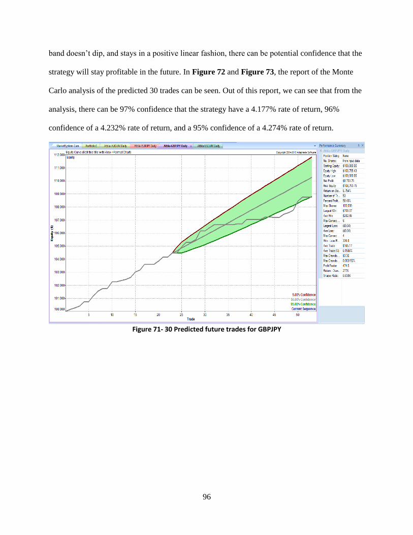
96
band doesn’t dip, and stays in a positive linear fashion, there can be potential confidence that the
strategy will stay profitable in the future. In Figure 72 and Figure 73, the report of the Monte
Carlo analysis of the predicted 30 trades can be seen. Out of this report, we can see that from the
analysis, there can be 97% confidence that the strategy have a 4.177% rate of return, 96%
confidence of a 4.232% rate of return, and a 95% confidence of a 4.274% rate of return.
Figure 71- 30 Predicted future trades for GBPJPY
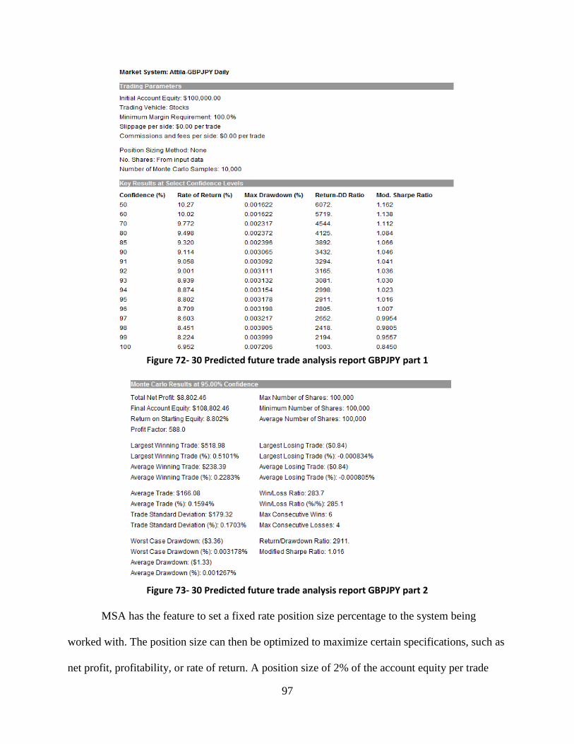
97
Figure 72- 30 Predicted future trade analysis report GBPJPY part 1
Figure 73- 30 Predicted future trade analysis report GBPJPY part 2
MSA has the feature to set a fixed rate position size percentage to the system being
worked with. The position size can then be optimized to maximize certain specifications, such as
net profit, profitability, or rate of return. A position size of 2% of the account equity per trade
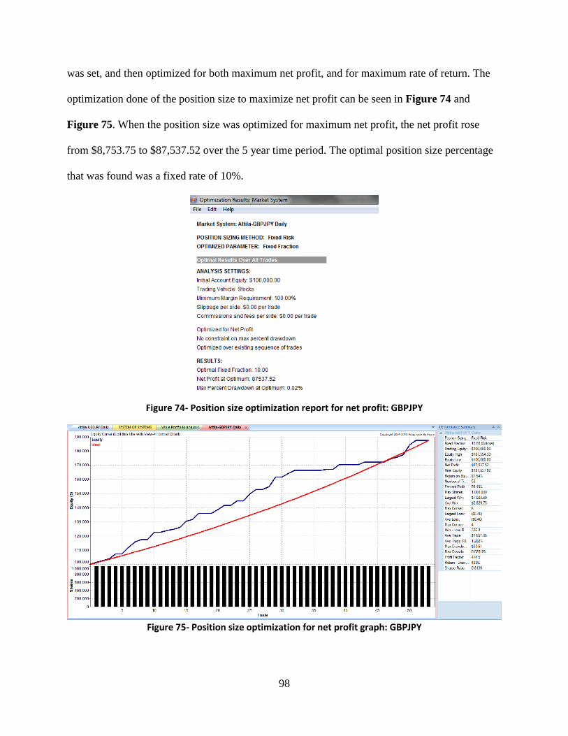
98
was set, and then optimized for both maximum net profit, and for maximum rate of return. The
optimization done of the position size to maximize net profit can be seen in Figure 74 and
Figure 75. When the position size was optimized for maximum net profit, the net profit rose
from $8,753.75 to $87,537.52 over the 5 year time period. The optimal position size percentage
that was found was a fixed rate of 10%.
Figure 74- Position size optimization report for net profit: GBPJPY
Figure 75- Position size optimization for net profit graph: GBPJPY
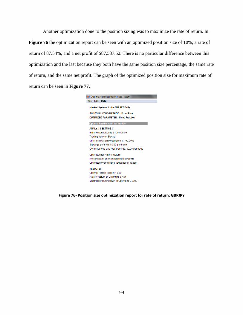
99
Another optimization done to the position sizing was to maximize the rate of return. In
Figure 76 the optimization report can be seen with an optimized position size of 10%, a rate of
return of 87.54%, and a net profit of $87,537.52. There is no particular difference between this
optimization and the last because they both have the same position size percentage, the same rate
of return, and the same net profit. The graph of the optimized position size for maximum rate of
return can be seen in Figure 77.
Figure 76- Position size optimization report for rate of return: GBPJPY
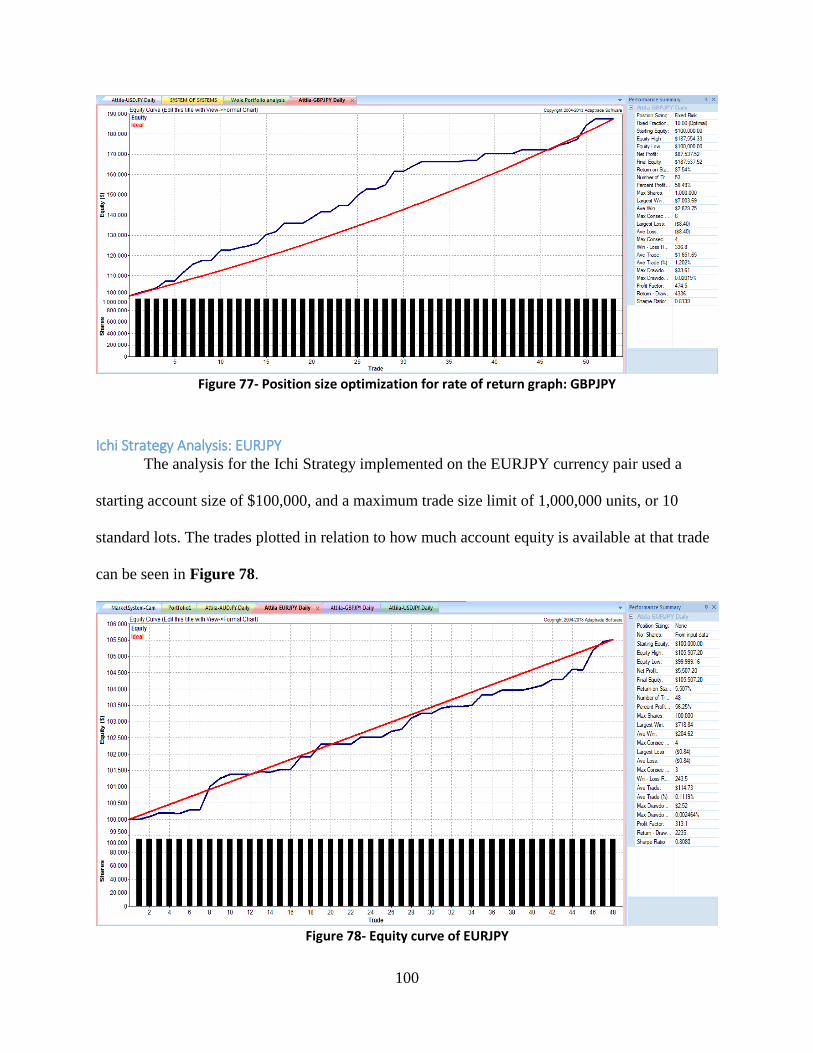
100
Figure 77- Position size optimization for rate of return graph: GBPJPY
Ichi Strategy Analysis: EURJPY The analysis for the Ichi Strategy implemented on the EURJPY currency pair used a
starting account size of $100,000, and a maximum trade size limit of 1,000,000 units, or 10
standard lots. The trades plotted in relation to how much account equity is available at that trade
can be seen in Figure 78.
Figure 78- Equity curve of EURJPY
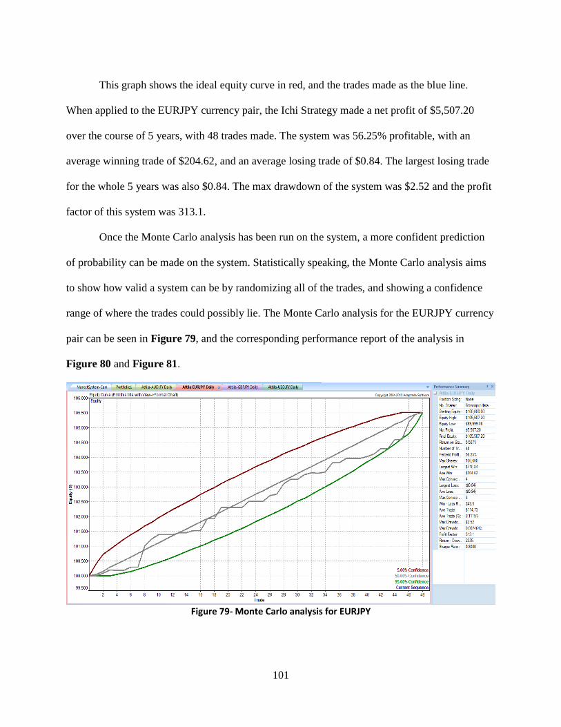
101
This graph shows the ideal equity curve in red, and the trades made as the blue line.
When applied to the EURJPY currency pair, the Ichi Strategy made a net profit of $5,507.20
over the course of 5 years, with 48 trades made. The system was 56.25% profitable, with an
average winning trade of $204.62, and an average losing trade of $0.84. The largest losing trade
for the whole 5 years was also $0.84. The max drawdown of the system was $2.52 and the profit
factor of this system was 313.1.
Once the Monte Carlo analysis has been run on the system, a more confident prediction
of probability can be made on the system. Statistically speaking, the Monte Carlo analysis aims
to show how valid a system can be by randomizing all of the trades, and showing a confidence
range of where the trades could possibly lie. The Monte Carlo analysis for the EURJPY currency
pair can be seen in Figure 79, and the corresponding performance report of the analysis in
Figure 80 and Figure 81.
Figure 79- Monte Carlo analysis for EURJPY
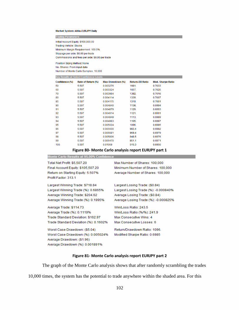
102
Figure 80- Monte Carlo analysis report EURJPY part 1
Figure 81- Monte Carlo analysis report EURJPY part 2
The graph of the Monte Carlo analysis shows that after randomly scrambling the trades
10,000 times, the system has the potential to trade anywhere within the shaded area. For this
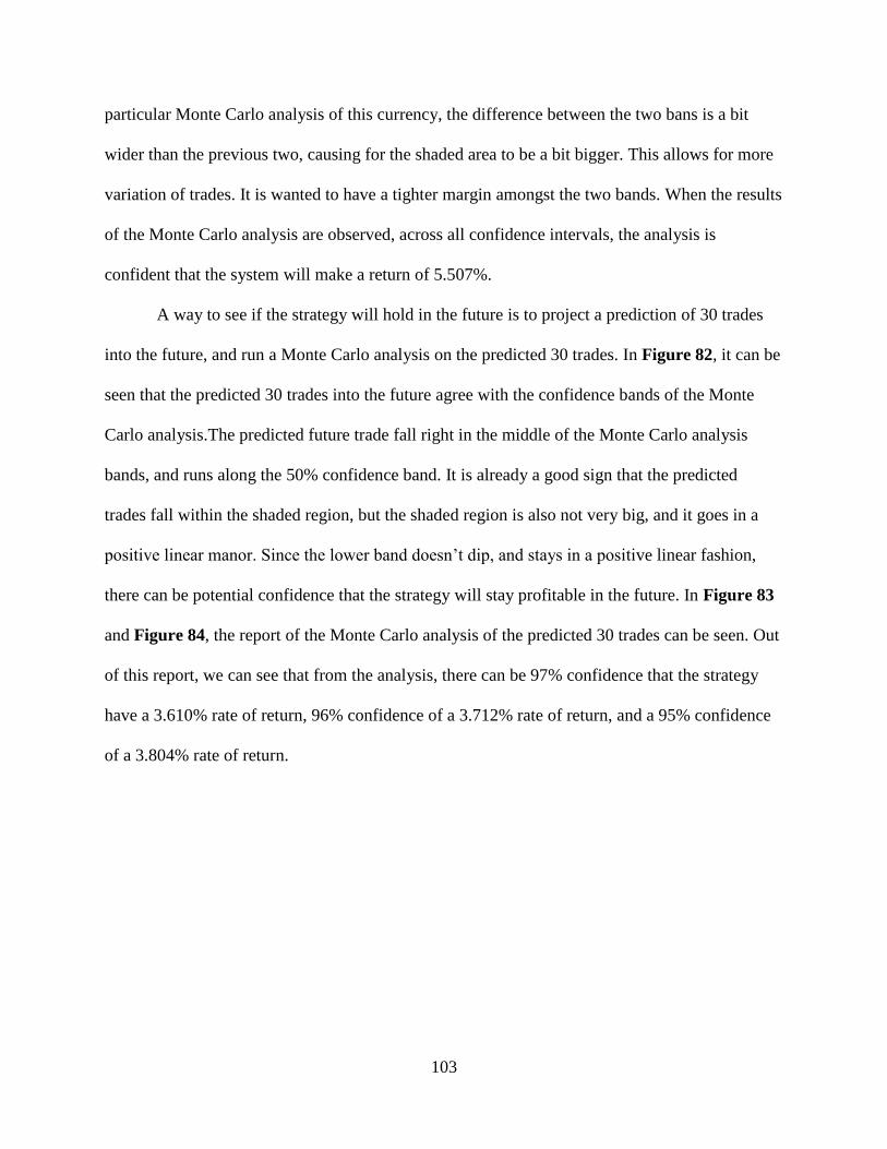
103
particular Monte Carlo analysis of this currency, the difference between the two bans is a bit
wider than the previous two, causing for the shaded area to be a bit bigger. This allows for more
variation of trades. It is wanted to have a tighter margin amongst the two bands. When the results
of the Monte Carlo analysis are observed, across all confidence intervals, the analysis is
confident that the system will make a return of 5.507%.
A way to see if the strategy will hold in the future is to project a prediction of 30 trades
into the future, and run a Monte Carlo analysis on the predicted 30 trades. In Figure 82, it can be
seen that the predicted 30 trades into the future agree with the confidence bands of the Monte
Carlo analysis.The predicted future trade fall right in the middle of the Monte Carlo analysis
bands, and runs along the 50% confidence band. It is already a good sign that the predicted
trades fall within the shaded region, but the shaded region is also not very big, and it goes in a
positive linear manor. Since the lower band doesn’t dip, and stays in a positive linear fashion,
there can be potential confidence that the strategy will stay profitable in the future. In Figure 83
and Figure 84, the report of the Monte Carlo analysis of the predicted 30 trades can be seen. Out
of this report, we can see that from the analysis, there can be 97% confidence that the strategy
have a 3.610% rate of return, 96% confidence of a 3.712% rate of return, and a 95% confidence
of a 3.804% rate of return.
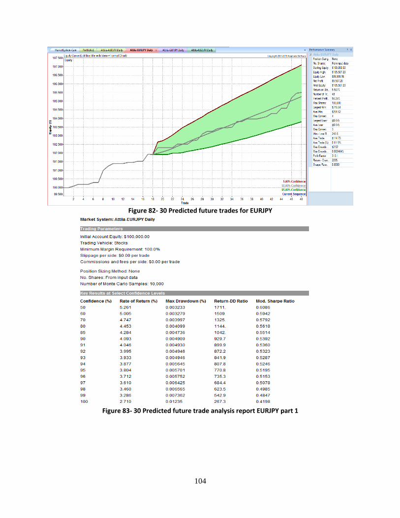
104
Figure 82- 30 Predicted future trades for EURJPY
Figure 83- 30 Predicted future trade analysis report EURJPY part 1
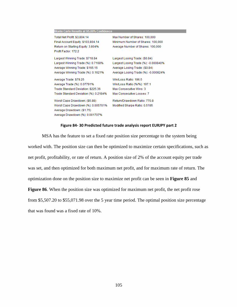
105
Figure 84- 30 Predicted future trade analysis report EURJPY part 2
MSA has the feature to set a fixed rate position size percentage to the system being
worked with. The position size can then be optimized to maximize certain specifications, such as
net profit, profitability, or rate of return. A position size of 2% of the account equity per trade
was set, and then optimized for both maximum net profit, and for maximum rate of return. The
optimization done on the position size to maximize net profit can be seen in Figure 85 and
Figure 86. When the position size was optimized for maximum net profit, the net profit rose
from $5,507.20 to $55,071.98 over the 5 year time period. The optimal position size percentage
that was found was a fixed rate of 10%.
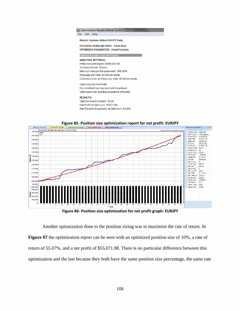
106
Figure 85- Position size optimization report for net profit: EURJPY
Figure 86- Position size optimization for net profit graph: EURJPY
Another optimization done to the position sizing was to maximize the rate of return. In
Figure 87 the optimization report can be seen with an optimized position size of 10%, a rate of
return of 55.07%, and a net profit of $55,071.98. There is no particular difference between this
optimization and the last because they both have the same position size percentage, the same rate
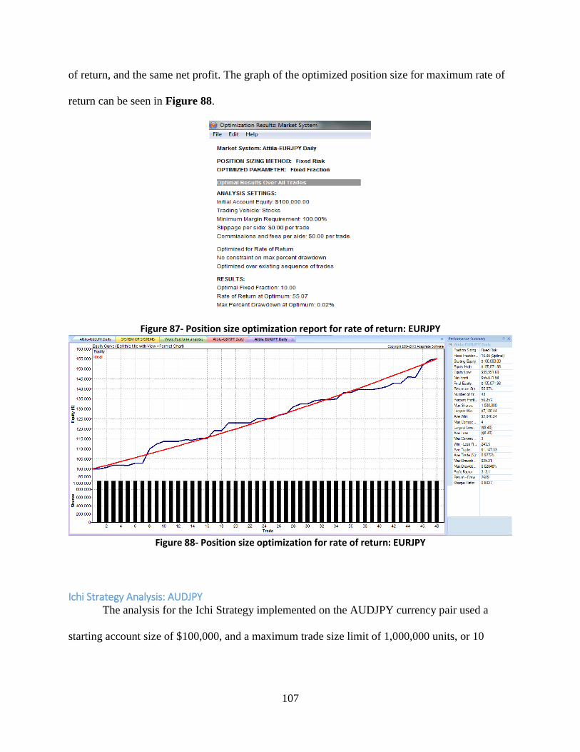
107
of return, and the same net profit. The graph of the optimized position size for maximum rate of
return can be seen in Figure 88.
Figure 87- Position size optimization report for rate of return: EURJPY
Figure 88- Position size optimization for rate of return: EURJPY
Ichi Strategy Analysis: AUDJPY The analysis for the Ichi Strategy implemented on the AUDJPY currency pair used a
starting account size of $100,000, and a maximum trade size limit of 1,000,000 units, or 10
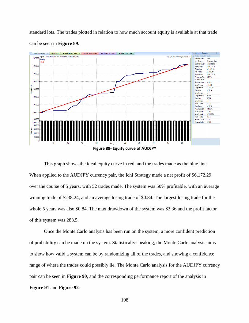
108
standard lots. The trades plotted in relation to how much account equity is available at that trade
can be seen in Figure 89.
Figure 89- Equity curve of AUDJPY
This graph shows the ideal equity curve in red, and the trades made as the blue line.
When applied to the AUDJPY currency pair, the Ichi Strategy made a net profit of $6,172.29
over the course of 5 years, with 52 trades made. The system was 50% profitable, with an average
winning trade of $238.24, and an average losing trade of $0.84. The largest losing trade for the
whole 5 years was also $0.84. The max drawdown of the system was $3.36 and the profit factor
of this system was 283.5.
Once the Monte Carlo analysis has been run on the system, a more confident prediction
of probability can be made on the system. Statistically speaking, the Monte Carlo analysis aims
to show how valid a system can be by randomizing all of the trades, and showing a confidence
range of where the trades could possibly lie. The Monte Carlo analysis for the AUDJPY currency
pair can be seen in Figure 90, and the corresponding performance report of the analysis in
Figure 91 and Figure 92.
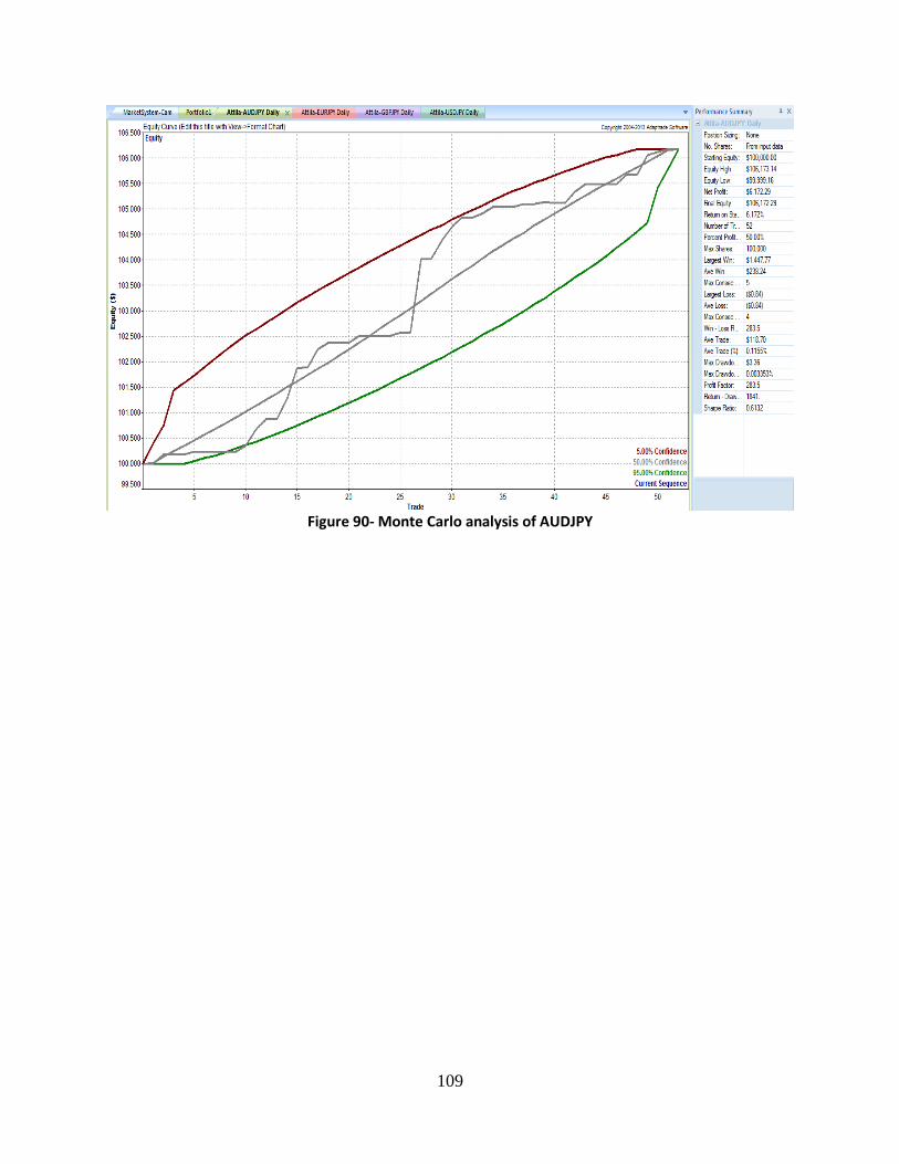
109
Figure 90- Monte Carlo analysis of AUDJPY
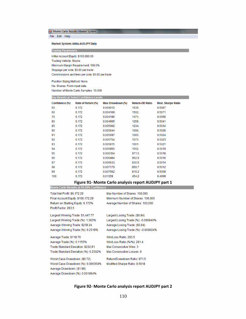
110
Figure 91- Monte Carlo analysis report AUDJPY part 1
Figure 92- Monte Carlo analysis report AUDJPY part 2
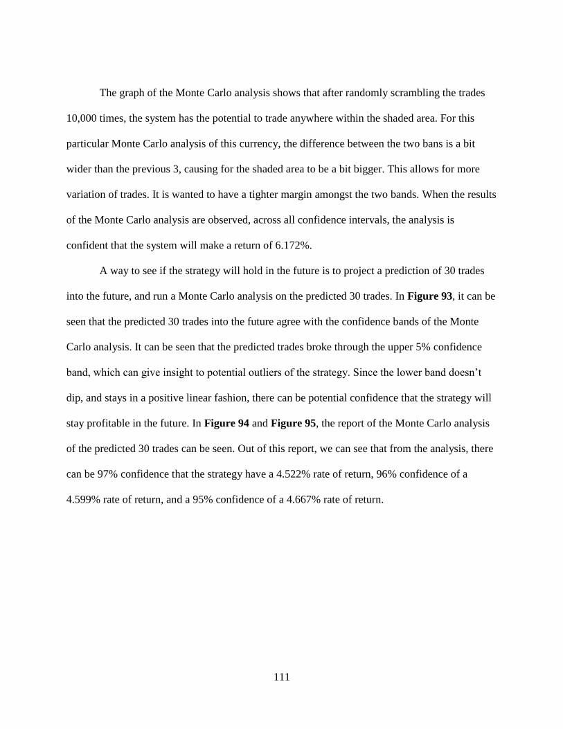
111
The graph of the Monte Carlo analysis shows that after randomly scrambling the trades
10,000 times, the system has the potential to trade anywhere within the shaded area. For this
particular Monte Carlo analysis of this currency, the difference between the two bans is a bit
wider than the previous 3, causing for the shaded area to be a bit bigger. This allows for more
variation of trades. It is wanted to have a tighter margin amongst the two bands. When the results
of the Monte Carlo analysis are observed, across all confidence intervals, the analysis is
confident that the system will make a return of 6.172%.
A way to see if the strategy will hold in the future is to project a prediction of 30 trades
into the future, and run a Monte Carlo analysis on the predicted 30 trades. In Figure 93, it can be
seen that the predicted 30 trades into the future agree with the confidence bands of the Monte
Carlo analysis. It can be seen that the predicted trades broke through the upper 5% confidence
band, which can give insight to potential outliers of the strategy. Since the lower band doesn’t
dip, and stays in a positive linear fashion, there can be potential confidence that the strategy will
stay profitable in the future. In Figure 94 and Figure 95, the report of the Monte Carlo analysis
of the predicted 30 trades can be seen. Out of this report, we can see that from the analysis, there
can be 97% confidence that the strategy have a 4.522% rate of return, 96% confidence of a
4.599% rate of return, and a 95% confidence of a 4.667% rate of return.
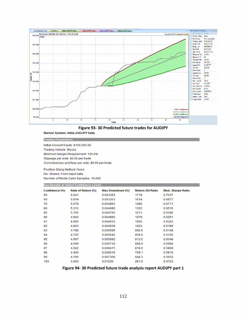
112
Figure 93- 30 Predicted future trades for AUDJPY
Figure 94- 30 Predicted future trade analysis report AUDJPY part 1
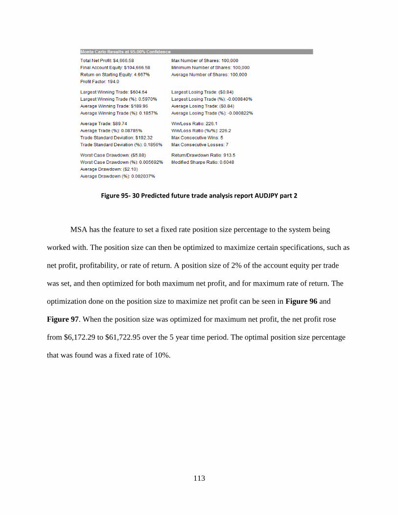
113
Figure 95- 30 Predicted future trade analysis report AUDJPY part 2
MSA has the feature to set a fixed rate position size percentage to the system being
worked with. The position size can then be optimized to maximize certain specifications, such as
net profit, profitability, or rate of return. A position size of 2% of the account equity per trade
was set, and then optimized for both maximum net profit, and for maximum rate of return. The
optimization done on the position size to maximize net profit can be seen in Figure 96 and
Figure 97. When the position size was optimized for maximum net profit, the net profit rose
from $6,172.29 to $61,722.95 over the 5 year time period. The optimal position size percentage
that was found was a fixed rate of 10%.
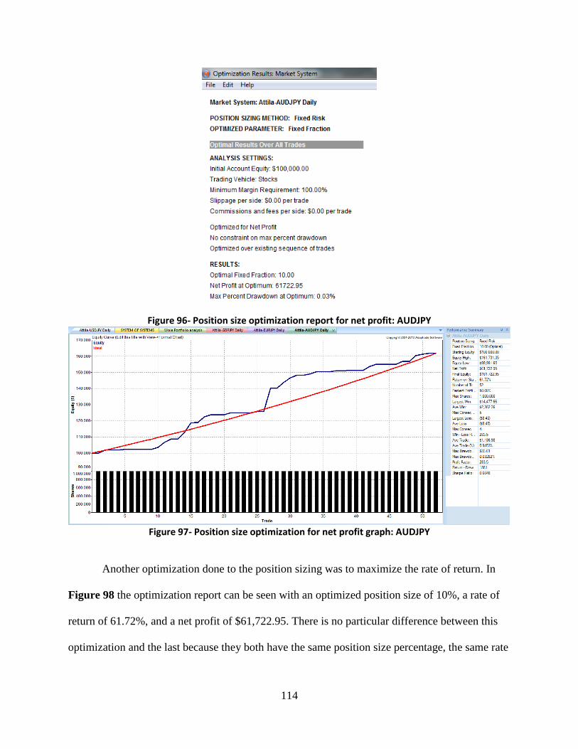
114
Figure 96- Position size optimization report for net profit: AUDJPY
Figure 97- Position size optimization for net profit graph: AUDJPY
Another optimization done to the position sizing was to maximize the rate of return. In
Figure 98 the optimization report can be seen with an optimized position size of 10%, a rate of
return of 61.72%, and a net profit of $61,722.95. There is no particular difference between this
optimization and the last because they both have the same position size percentage, the same rate
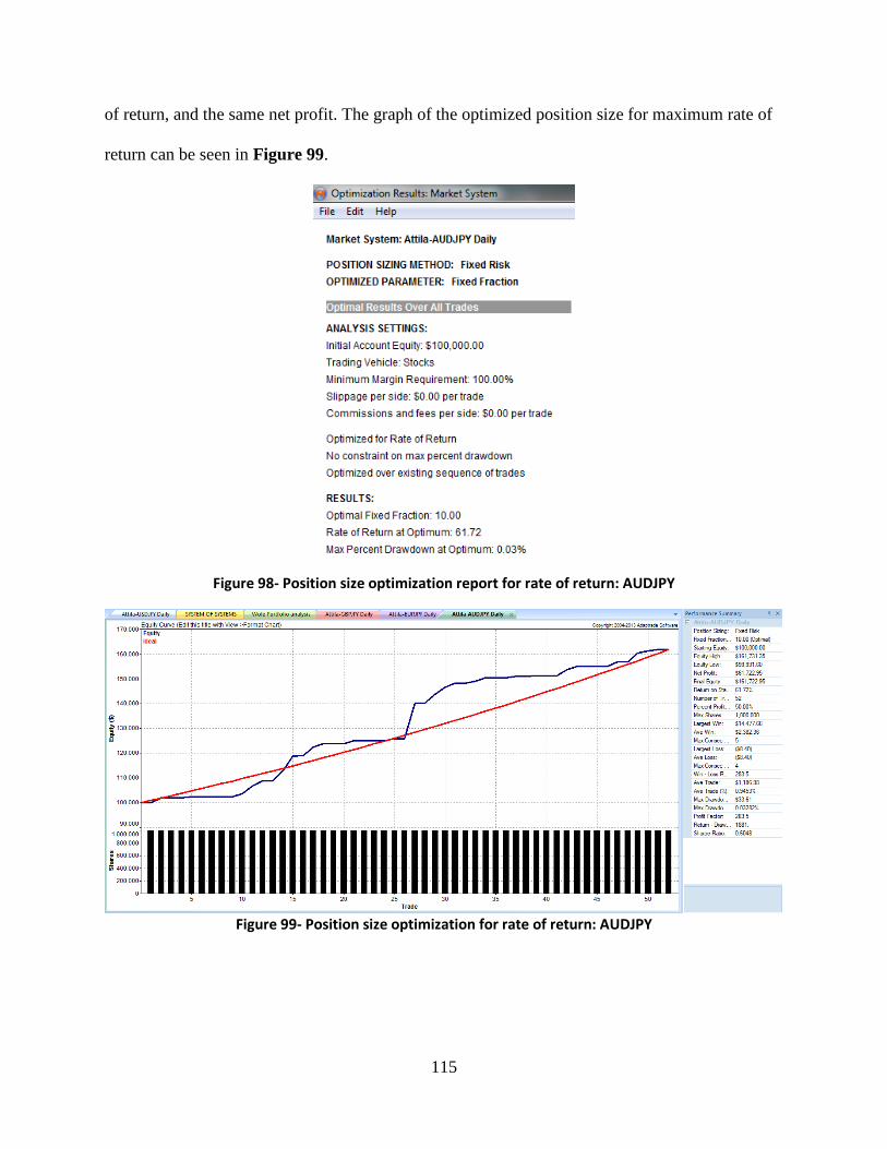
115
of return, and the same net profit. The graph of the optimized position size for maximum rate of
return can be seen in Figure 99.
Figure 98- Position size optimization report for rate of return: AUDJPY
Figure 99- Position size optimization for rate of return: AUDJPY
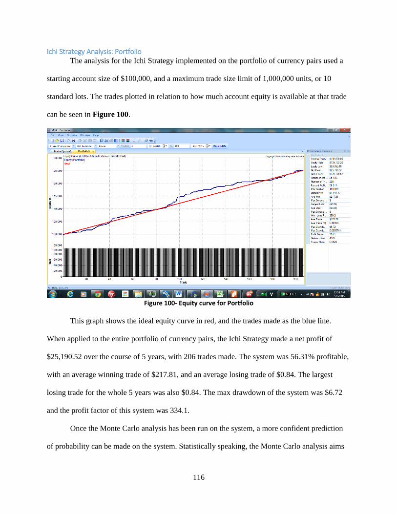
116
Ichi Strategy Analysis: Portfolio The analysis for the Ichi Strategy implemented on the portfolio of currency pairs used a
starting account size of $100,000, and a maximum trade size limit of 1,000,000 units, or 10
standard lots. The trades plotted in relation to how much account equity is available at that trade
can be seen in Figure 100.
Figure 100- Equity curve for Portfolio
This graph shows the ideal equity curve in red, and the trades made as the blue line.
When applied to the entire portfolio of currency pairs, the Ichi Strategy made a net profit of
$25,190.52 over the course of 5 years, with 206 trades made. The system was 56.31% profitable,
with an average winning trade of $217.81, and an average losing trade of $0.84. The largest
losing trade for the whole 5 years was also $0.84. The max drawdown of the system was $6.72
and the profit factor of this system was 334.1.
Once the Monte Carlo analysis has been run on the system, a more confident prediction
of probability can be made on the system. Statistically speaking, the Monte Carlo analysis aims
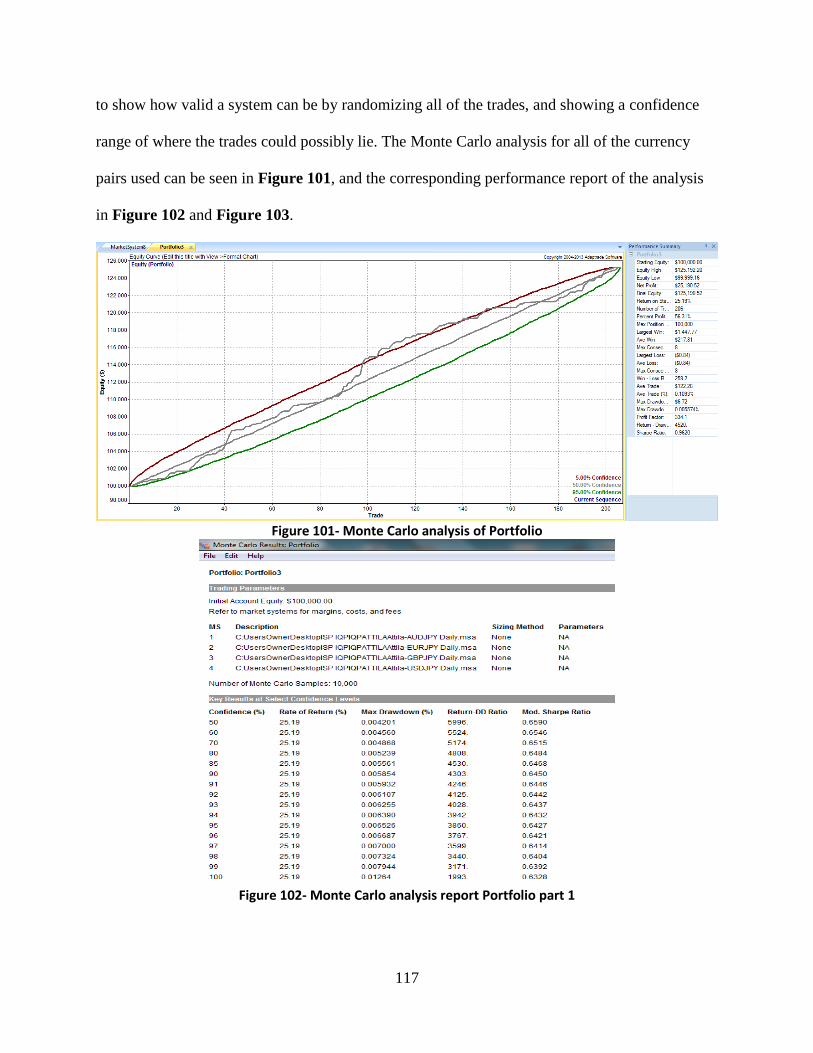
117
to show how valid a system can be by randomizing all of the trades, and showing a confidence
range of where the trades could possibly lie. The Monte Carlo analysis for all of the currency
pairs used can be seen in Figure 101, and the corresponding performance report of the analysis
in Figure 102 and Figure 103.
Figure 101- Monte Carlo analysis of Portfolio
Figure 102- Monte Carlo analysis report Portfolio part 1
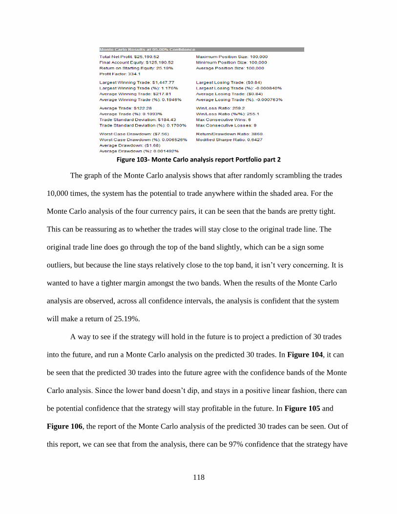
118
Figure 103- Monte Carlo analysis report Portfolio part 2
The graph of the Monte Carlo analysis shows that after randomly scrambling the trades
10,000 times, the system has the potential to trade anywhere within the shaded area. For the
Monte Carlo analysis of the four currency pairs, it can be seen that the bands are pretty tight.
This can be reassuring as to whether the trades will stay close to the original trade line. The
original trade line does go through the top of the band slightly, which can be a sign some
outliers, but because the line stays relatively close to the top band, it isn’t very concerning. It is
wanted to have a tighter margin amongst the two bands. When the results of the Monte Carlo
analysis are observed, across all confidence intervals, the analysis is confident that the system
will make a return of 25.19%.
A way to see if the strategy will hold in the future is to project a prediction of 30 trades
into the future, and run a Monte Carlo analysis on the predicted 30 trades. In Figure 104, it can
be seen that the predicted 30 trades into the future agree with the confidence bands of the Monte
Carlo analysis. Since the lower band doesn’t dip, and stays in a positive linear fashion, there can
be potential confidence that the strategy will stay profitable in the future. In Figure 105 and
Figure 106, the report of the Monte Carlo analysis of the predicted 30 trades can be seen. Out of
this report, we can see that from the analysis, there can be 97% confidence that the strategy have
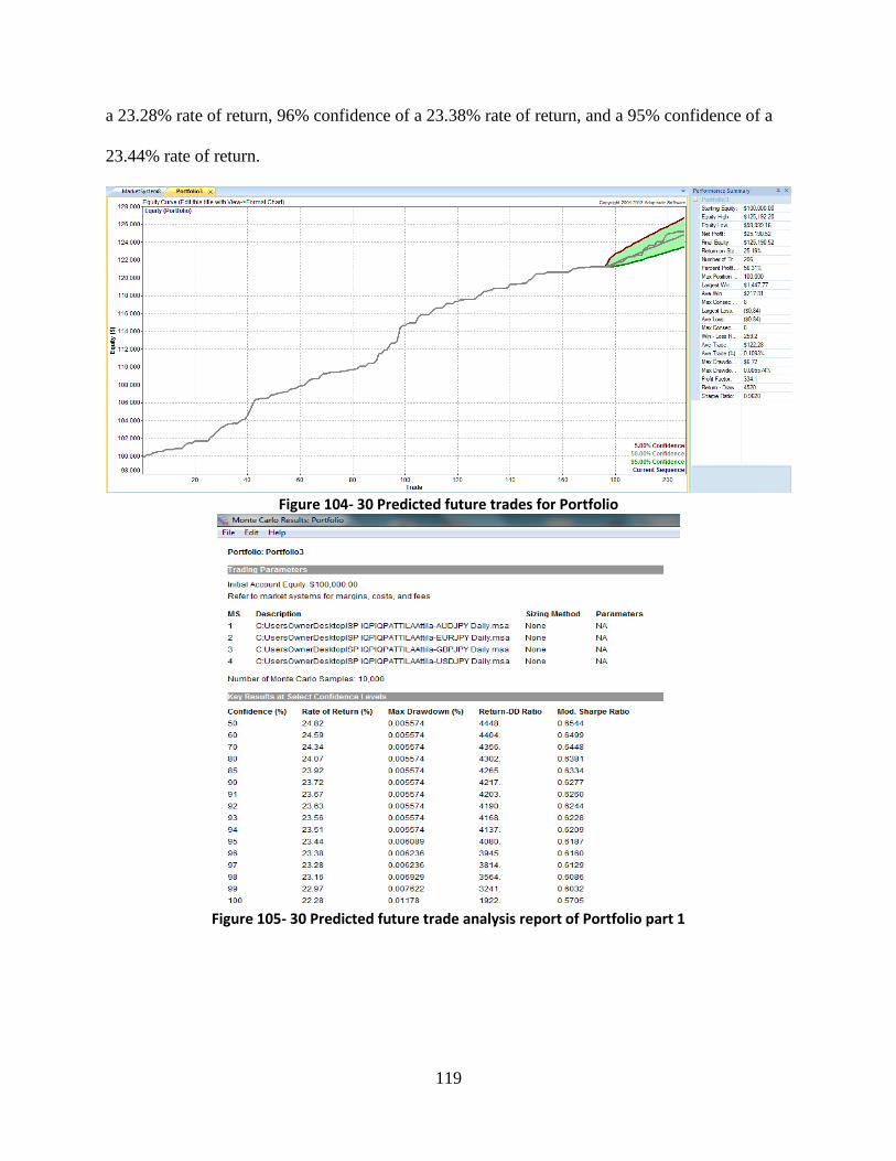
119
a 23.28% rate of return, 96% confidence of a 23.38% rate of return, and a 95% confidence of a
23.44% rate of return.
Figure 104- 30 Predicted future trades for Portfolio
Figure 105- 30 Predicted future trade analysis report of Portfolio part 1
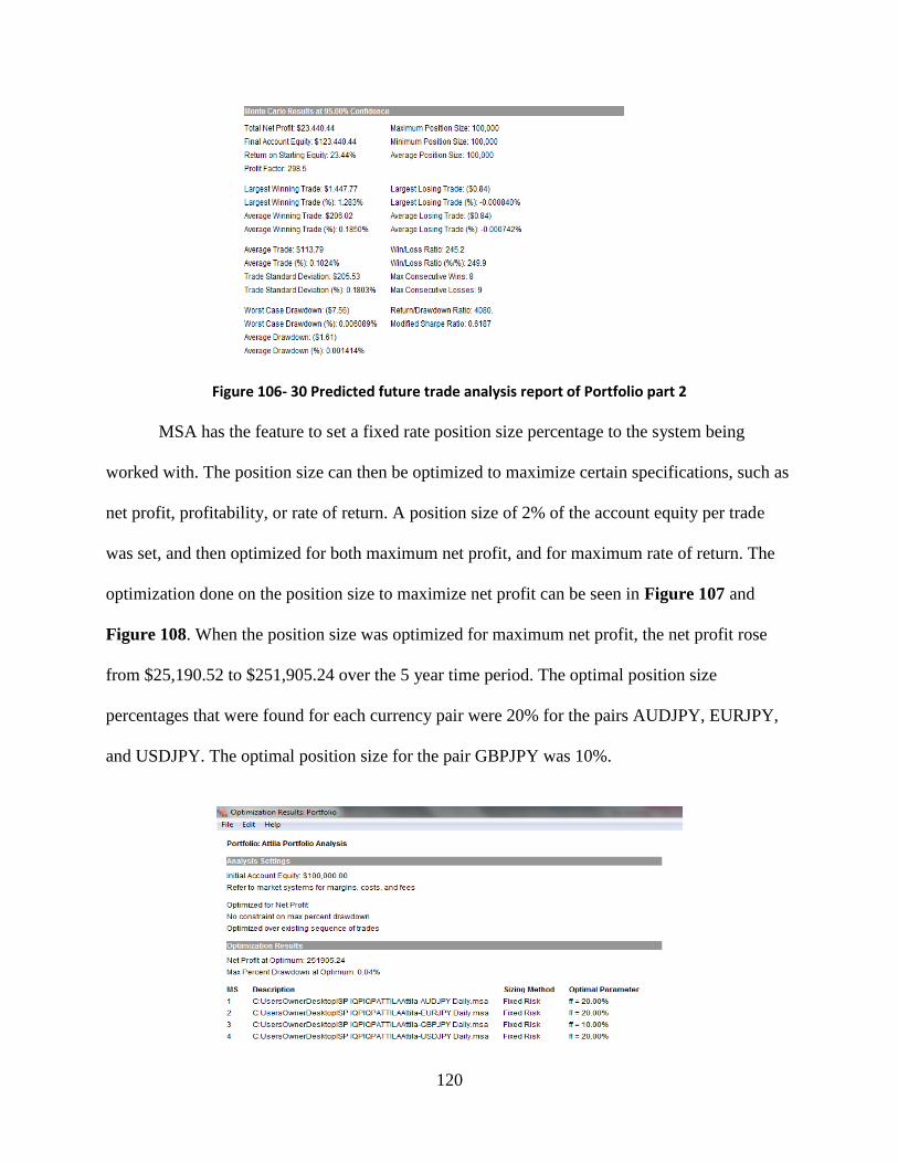
120
Figure 106- 30 Predicted future trade analysis report of Portfolio part 2
MSA has the feature to set a fixed rate position size percentage to the system being
worked with. The position size can then be optimized to maximize certain specifications, such as
net profit, profitability, or rate of return. A position size of 2% of the account equity per trade
was set, and then optimized for both maximum net profit, and for maximum rate of return. The
optimization done on the position size to maximize net profit can be seen in Figure 107 and
Figure 108. When the position size was optimized for maximum net profit, the net profit rose
from $25,190.52 to $251,905.24 over the 5 year time period. The optimal position size
percentages that were found for each currency pair were 20% for the pairs AUDJPY, EURJPY,
and USDJPY. The optimal position size for the pair GBPJPY was 10%.
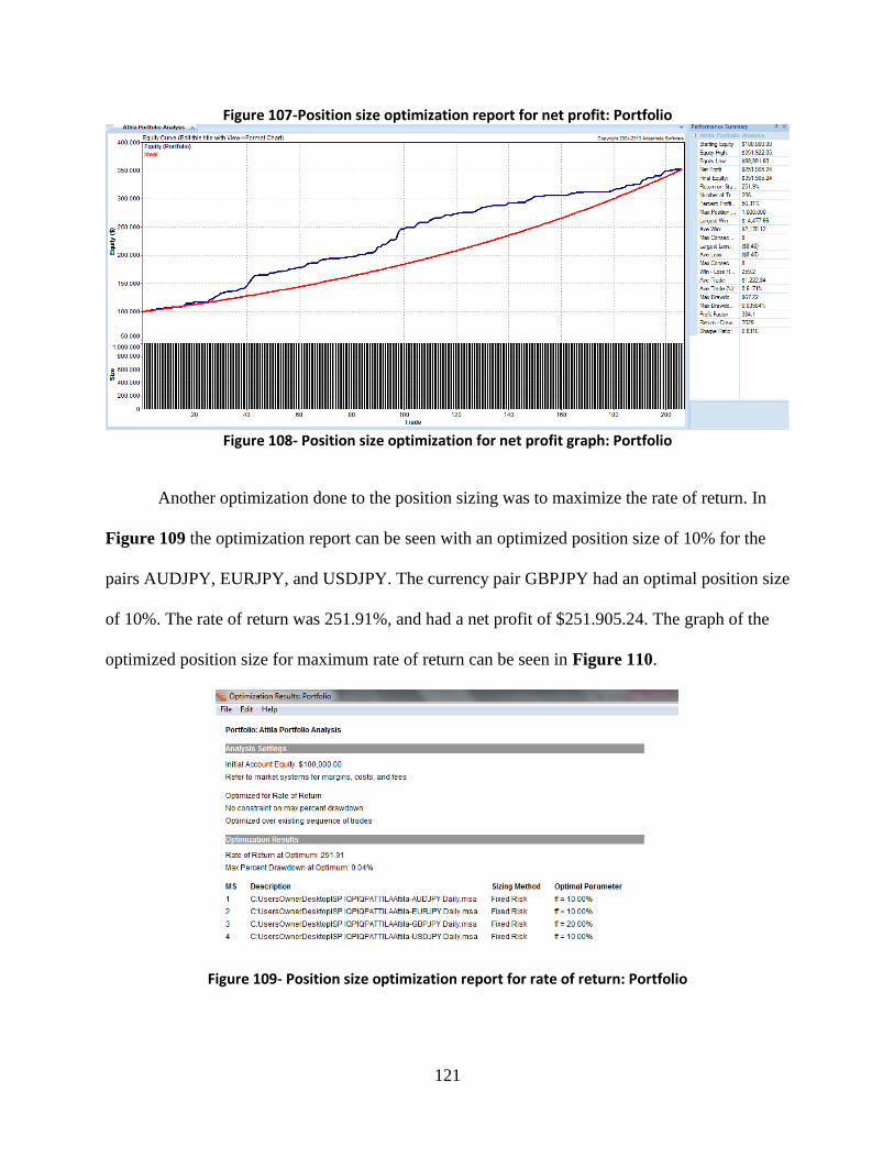
121
Figure 107-Position size optimization report for net profit: Portfolio
Figure 108- Position size optimization for net profit graph: Portfolio
Another optimization done to the position sizing was to maximize the rate of return. In
Figure 109 the optimization report can be seen with an optimized position size of 10% for the
pairs AUDJPY, EURJPY, and USDJPY. The currency pair GBPJPY had an optimal position size
of 10%. The rate of return was 251.91%, and had a net profit of $251.905.24. The graph of the
optimized position size for maximum rate of return can be seen in Figure 110.
Figure 109- Position size optimization report for rate of return: Portfolio
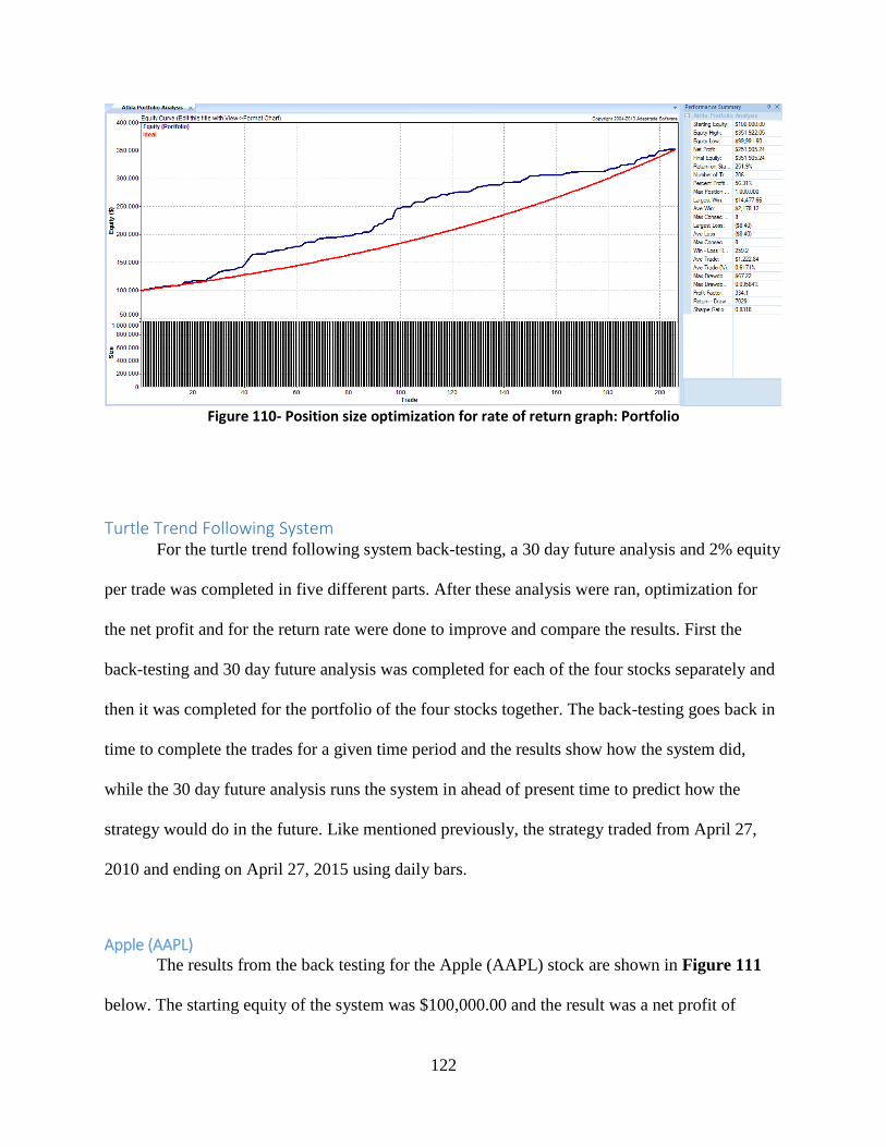
122
Figure 110- Position size optimization for rate of return graph: Portfolio
Turtle Trend Following System For the turtle trend following system back-testing, a 30 day future analysis and 2% equity
per trade was completed in five different parts. After these analysis were ran, optimization for
the net profit and for the return rate were done to improve and compare the results. First the
back-testing and 30 day future analysis was completed for each of the four stocks separately and
then it was completed for the portfolio of the four stocks together. The back-testing goes back in
time to complete the trades for a given time period and the results show how the system did,
while the 30 day future analysis runs the system in ahead of present time to predict how the
strategy would do in the future. Like mentioned previously, the strategy traded from April 27,
2010 and ending on April 27, 2015 using daily bars.
Apple (AAPL) The results from the back testing for the Apple (AAPL) stock are shown in Figure 111
below. The starting equity of the system was $100,000.00 and the result was a net profit of
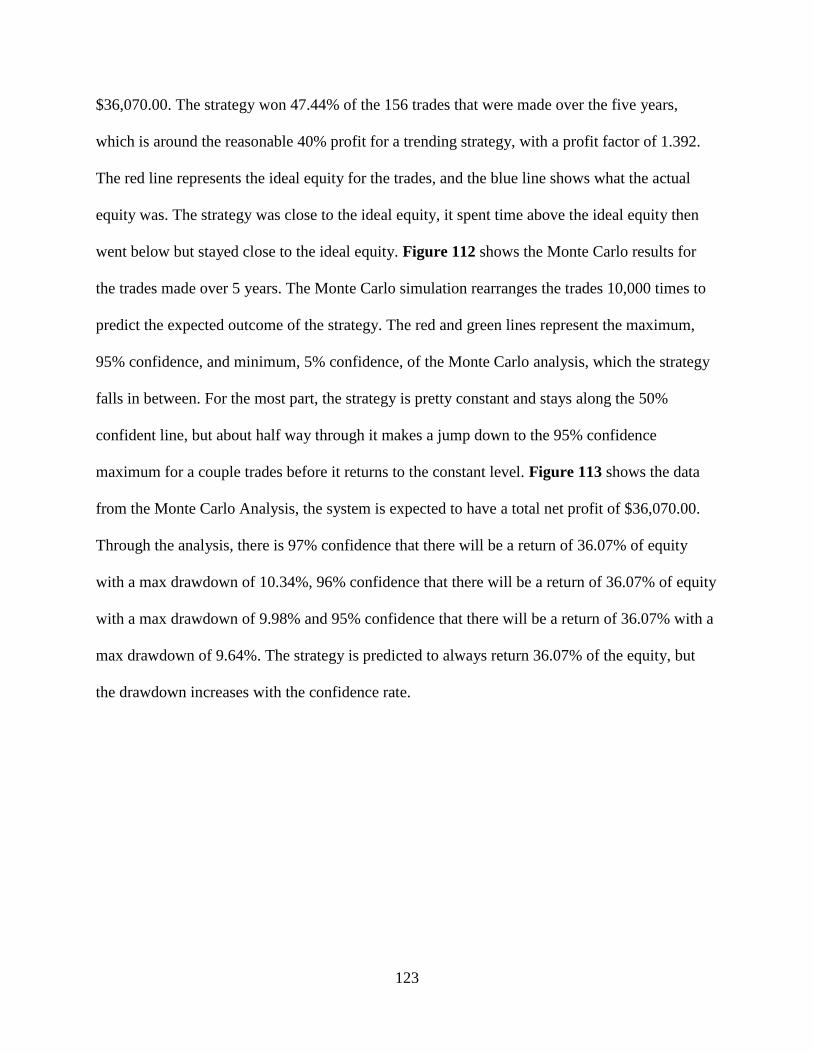
123
$36,070.00. The strategy won 47.44% of the 156 trades that were made over the five years,
which is around the reasonable 40% profit for a trending strategy, with a profit factor of 1.392.
The red line represents the ideal equity for the trades, and the blue line shows what the actual
equity was. The strategy was close to the ideal equity, it spent time above the ideal equity then
went below but stayed close to the ideal equity. Figure 112 shows the Monte Carlo results for
the trades made over 5 years. The Monte Carlo simulation rearranges the trades 10,000 times to
predict the expected outcome of the strategy. The red and green lines represent the maximum,
95% confidence, and minimum, 5% confidence, of the Monte Carlo analysis, which the strategy
falls in between. For the most part, the strategy is pretty constant and stays along the 50%
confident line, but about half way through it makes a jump down to the 95% confidence
maximum for a couple trades before it returns to the constant level. Figure 113 shows the data
from the Monte Carlo Analysis, the system is expected to have a total net profit of $36,070.00.
Through the analysis, there is 97% confidence that there will be a return of 36.07% of equity
with a max drawdown of 10.34%, 96% confidence that there will be a return of 36.07% of equity
with a max drawdown of 9.98% and 95% confidence that there will be a return of 36.07% with a
max drawdown of 9.64%. The strategy is predicted to always return 36.07% of the equity, but
the drawdown increases with the confidence rate.
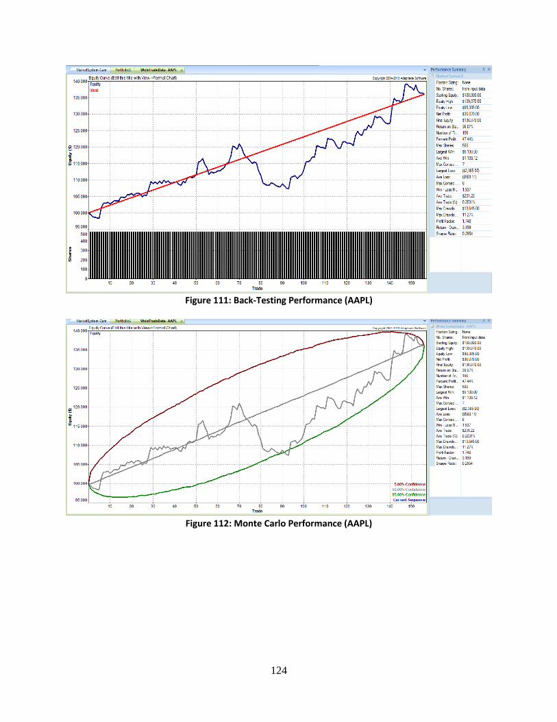
124
Figure 111: Back-Testing Performance (AAPL)
Figure 112: Monte Carlo Performance (AAPL)
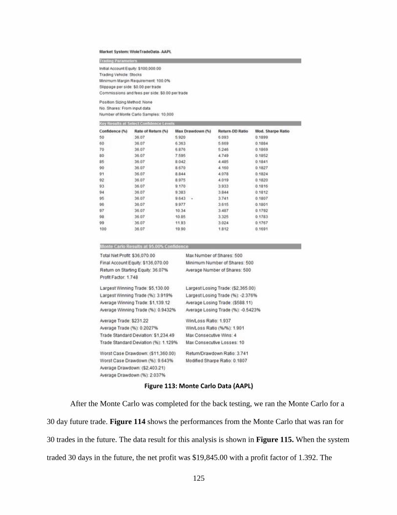
125
Figure 113: Monte Carlo Data (AAPL)
After the Monte Carlo was completed for the back testing, we ran the Monte Carlo for a
30 day future trade. Figure 114 shows the performances from the Monte Carlo that was ran for
30 trades in the future. The data result for this analysis is shown in Figure 115. When the system
traded 30 days in the future, the net profit was $19,845.00 with a profit factor of 1.392. The
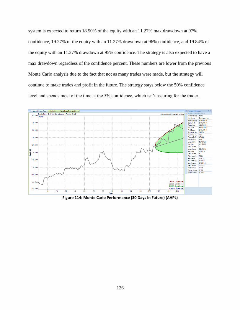
126
system is expected to return 18.50% of the equity with an 11.27% max drawdown at 97%
confidence, 19.27% of the equity with an 11.27% drawdown at 96% confidence, and 19.84% of
the equity with an 11.27% drawdown at 95% confidence. The strategy is also expected to have a
max drawdown regardless of the confidence percent. These numbers are lower from the previous
Monte Carlo analysis due to the fact that not as many trades were made, but the strategy will
continue to make trades and profit in the future. The strategy stays below the 50% confidence
level and spends most of the time at the 5% confidence, which isn’t assuring for the trader.
Figure 114: Monte Carlo Performance (30 Days In Future) (AAPL)
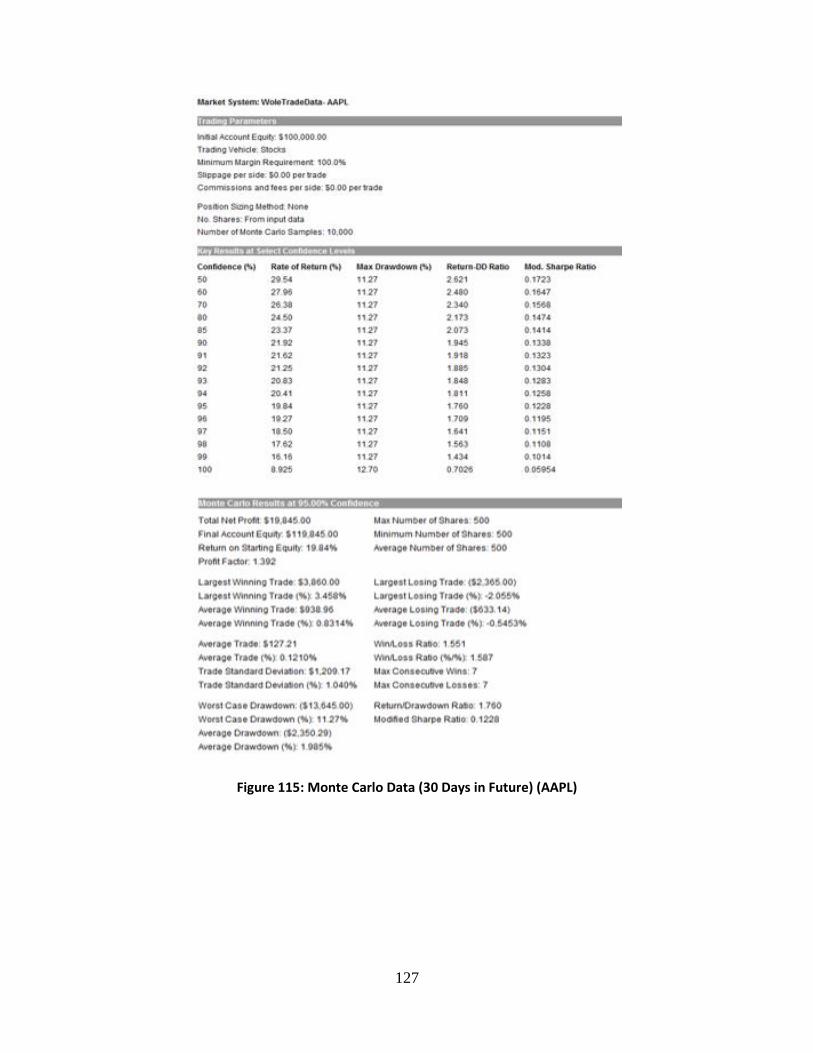
127
Figure 115: Monte Carlo Data (30 Days in Future) (AAPL)
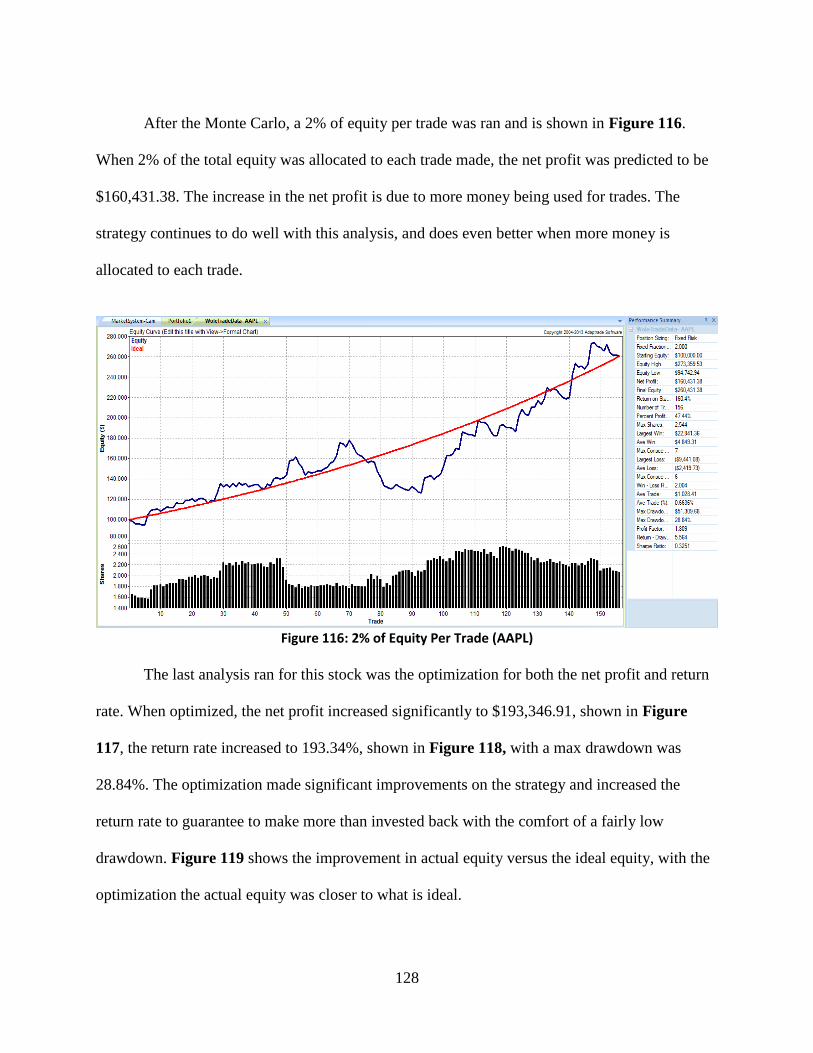
128
After the Monte Carlo, a 2% of equity per trade was ran and is shown in Figure 116.
When 2% of the total equity was allocated to each trade made, the net profit was predicted to be
$160,431.38. The increase in the net profit is due to more money being used for trades. The
strategy continues to do well with this analysis, and does even better when more money is
allocated to each trade.
Figure 116: 2% of Equity Per Trade (AAPL)
The last analysis ran for this stock was the optimization for both the net profit and return
rate. When optimized, the net profit increased significantly to $193,346.91, shown in Figure
117, the return rate increased to 193.34%, shown in Figure 118, with a max drawdown was
28.84%. The optimization made significant improvements on the strategy and increased the
return rate to guarantee to make more than invested back with the comfort of a fairly low
drawdown. Figure 119 shows the improvement in actual equity versus the ideal equity, with the
optimization the actual equity was closer to what is ideal.
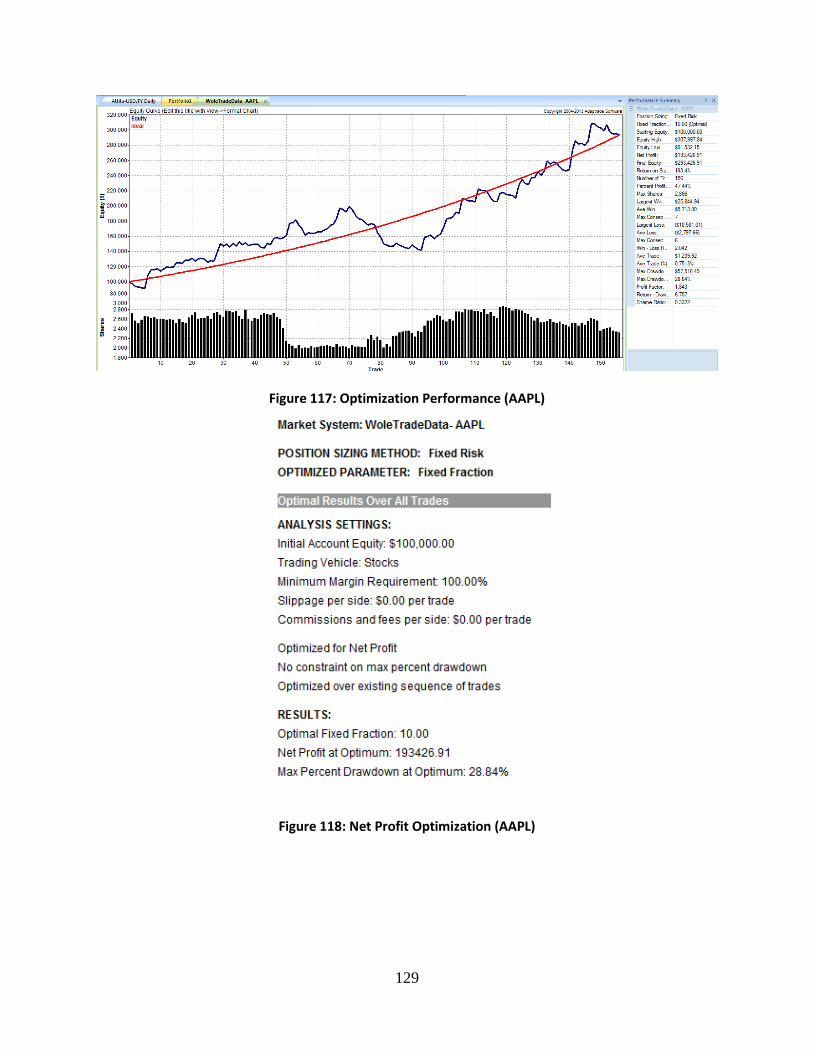
129
Figure 117: Optimization Performance (AAPL)
Figure 118: Net Profit Optimization (AAPL)
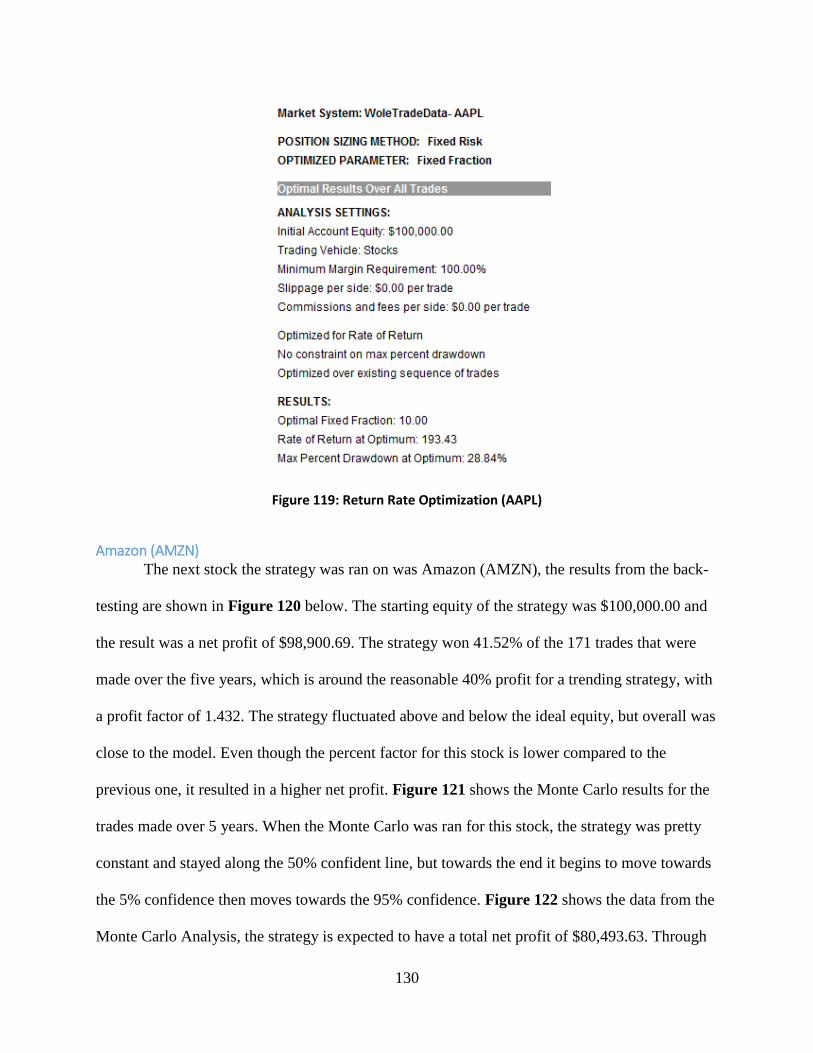
130
Figure 119: Return Rate Optimization (AAPL)
Amazon (AMZN) The next stock the strategy was ran on was Amazon (AMZN), the results from the back-
testing are shown in Figure 120 below. The starting equity of the strategy was $100,000.00 and
the result was a net profit of $98,900.69. The strategy won 41.52% of the 171 trades that were
made over the five years, which is around the reasonable 40% profit for a trending strategy, with
a profit factor of 1.432. The strategy fluctuated above and below the ideal equity, but overall was
close to the model. Even though the percent factor for this stock is lower compared to the
previous one, it resulted in a higher net profit. Figure 121 shows the Monte Carlo results for the
trades made over 5 years. When the Monte Carlo was ran for this stock, the strategy was pretty
constant and stayed along the 50% confident line, but towards the end it begins to move towards
the 5% confidence then moves towards the 95% confidence. Figure 122 shows the data from the
Monte Carlo Analysis, the strategy is expected to have a total net profit of $80,493.63. Through
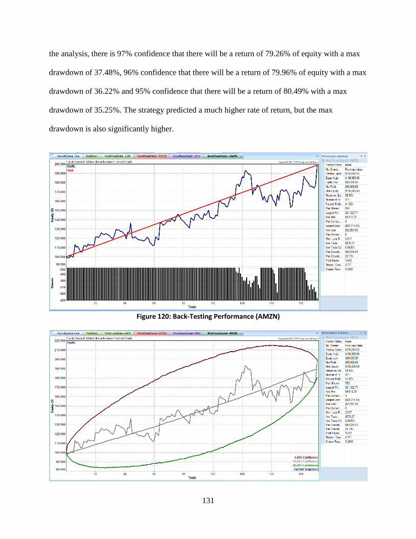
131
the analysis, there is 97% confidence that there will be a return of 79.26% of equity with a max
drawdown of 37.48%, 96% confidence that there will be a return of 79.96% of equity with a max
drawdown of 36.22% and 95% confidence that there will be a return of 80.49% with a max
drawdown of 35.25%. The strategy predicted a much higher rate of return, but the max
drawdown is also significantly higher.
Figure 120: Back-Testing Performance (AMZN)
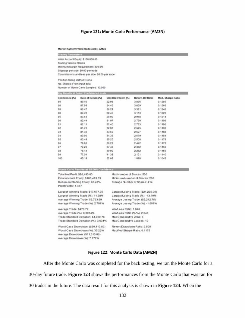
132
Figure 121: Monte Carlo Performance (AMZN)
Figure 122: Monte Carlo Data (AMZN)
After the Monte Carlo was completed for the back testing, we ran the Monte Carlo for a
30-day future trade. Figure 123 shows the performances from the Monte Carlo that was ran for
30 trades in the future. The data result for this analysis is shown in Figure 124. When the
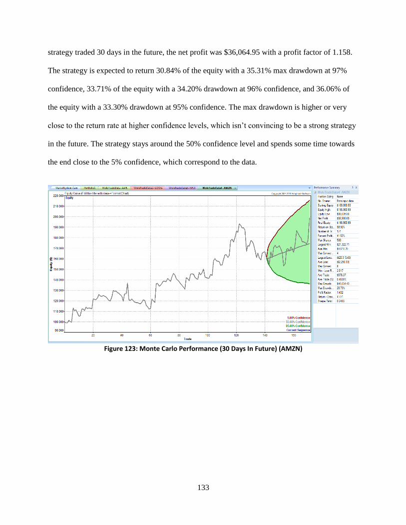
133
strategy traded 30 days in the future, the net profit was $36,064.95 with a profit factor of 1.158.
The strategy is expected to return 30.84% of the equity with a 35.31% max drawdown at 97%
confidence, 33.71% of the equity with a 34.20% drawdown at 96% confidence, and 36.06% of
the equity with a 33.30% drawdown at 95% confidence. The max drawdown is higher or very
close to the return rate at higher confidence levels, which isn’t convincing to be a strong strategy
in the future. The strategy stays around the 50% confidence level and spends some time towards
the end close to the 5% confidence, which correspond to the data.
Figure 123: Monte Carlo Performance (30 Days In Future) (AMZN)
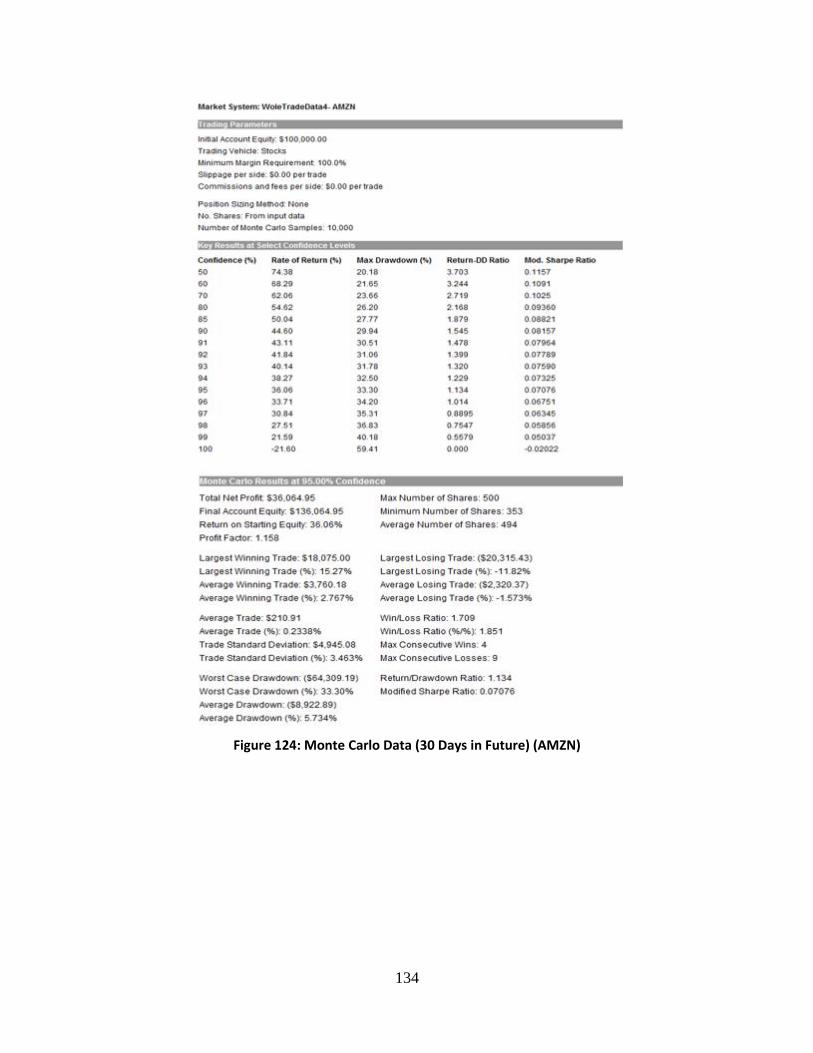
134
Figure 124: Monte Carlo Data (30 Days in Future) (AMZN)
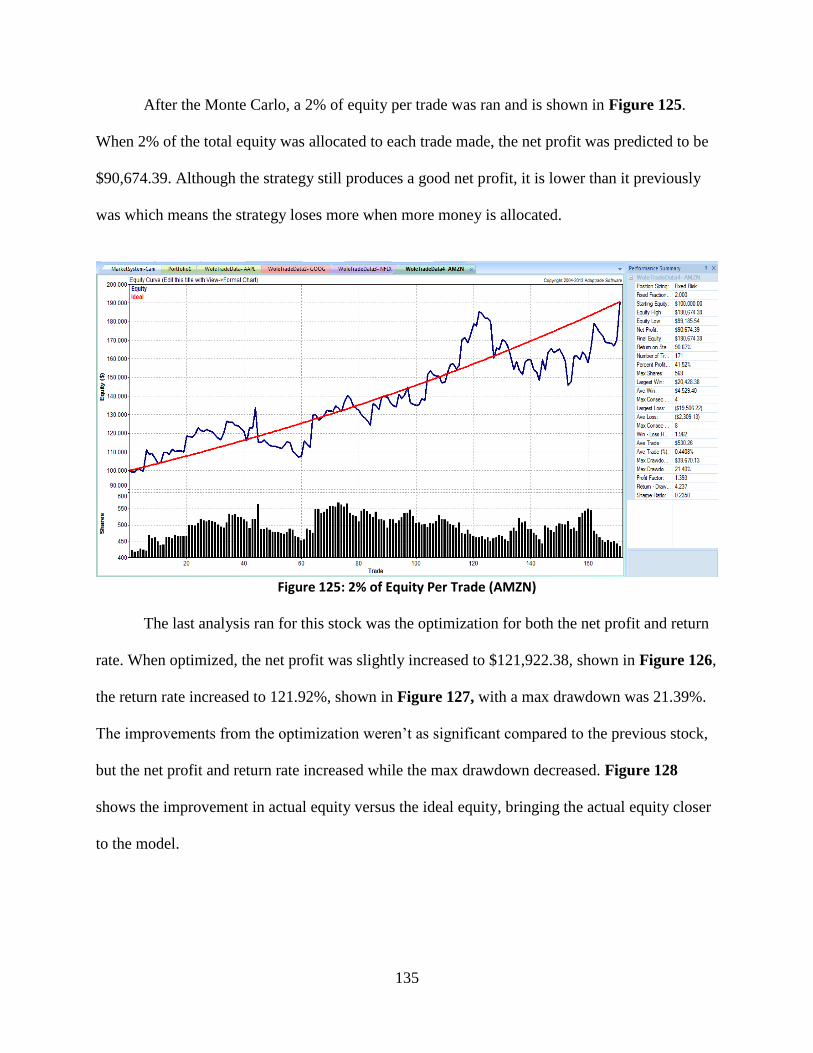
135
After the Monte Carlo, a 2% of equity per trade was ran and is shown in Figure 125.
When 2% of the total equity was allocated to each trade made, the net profit was predicted to be
$90,674.39. Although the strategy still produces a good net profit, it is lower than it previously
was which means the strategy loses more when more money is allocated.
Figure 125: 2% of Equity Per Trade (AMZN)
The last analysis ran for this stock was the optimization for both the net profit and return
rate. When optimized, the net profit was slightly increased to $121,922.38, shown in Figure 126,
the return rate increased to 121.92%, shown in Figure 127, with a max drawdown was 21.39%.
The improvements from the optimization weren’t as significant compared to the previous stock,
but the net profit and return rate increased while the max drawdown decreased. Figure 128
shows the improvement in actual equity versus the ideal equity, bringing the actual equity closer
to the model.
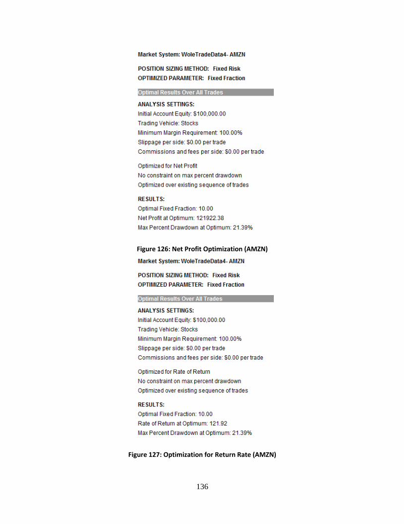
136
Figure 126: Net Profit Optimization (AMZN)
Figure 127: Optimization for Return Rate (AMZN)
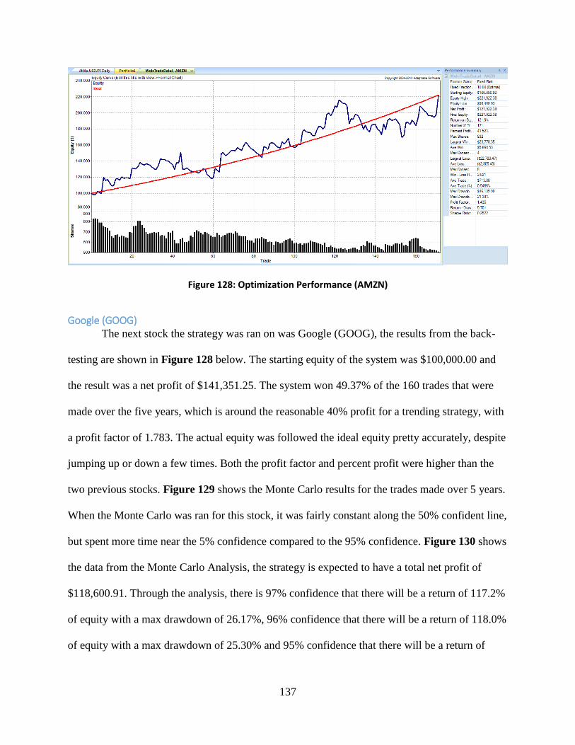
137
Figure 128: Optimization Performance (AMZN)
Google (GOOG) The next stock the strategy was ran on was Google (GOOG), the results from the back-
testing are shown in Figure 128 below. The starting equity of the system was $100,000.00 and
the result was a net profit of $141,351.25. The system won 49.37% of the 160 trades that were
made over the five years, which is around the reasonable 40% profit for a trending strategy, with
a profit factor of 1.783. The actual equity was followed the ideal equity pretty accurately, despite
jumping up or down a few times. Both the profit factor and percent profit were higher than the
two previous stocks. Figure 129 shows the Monte Carlo results for the trades made over 5 years.
When the Monte Carlo was ran for this stock, it was fairly constant along the 50% confident line,
but spent more time near the 5% confidence compared to the 95% confidence. Figure 130 shows
the data from the Monte Carlo Analysis, the strategy is expected to have a total net profit of
$118,600.91. Through the analysis, there is 97% confidence that there will be a return of 117.2%
of equity with a max drawdown of 26.17%, 96% confidence that there will be a return of 118.0%
of equity with a max drawdown of 25.30% and 95% confidence that there will be a return of
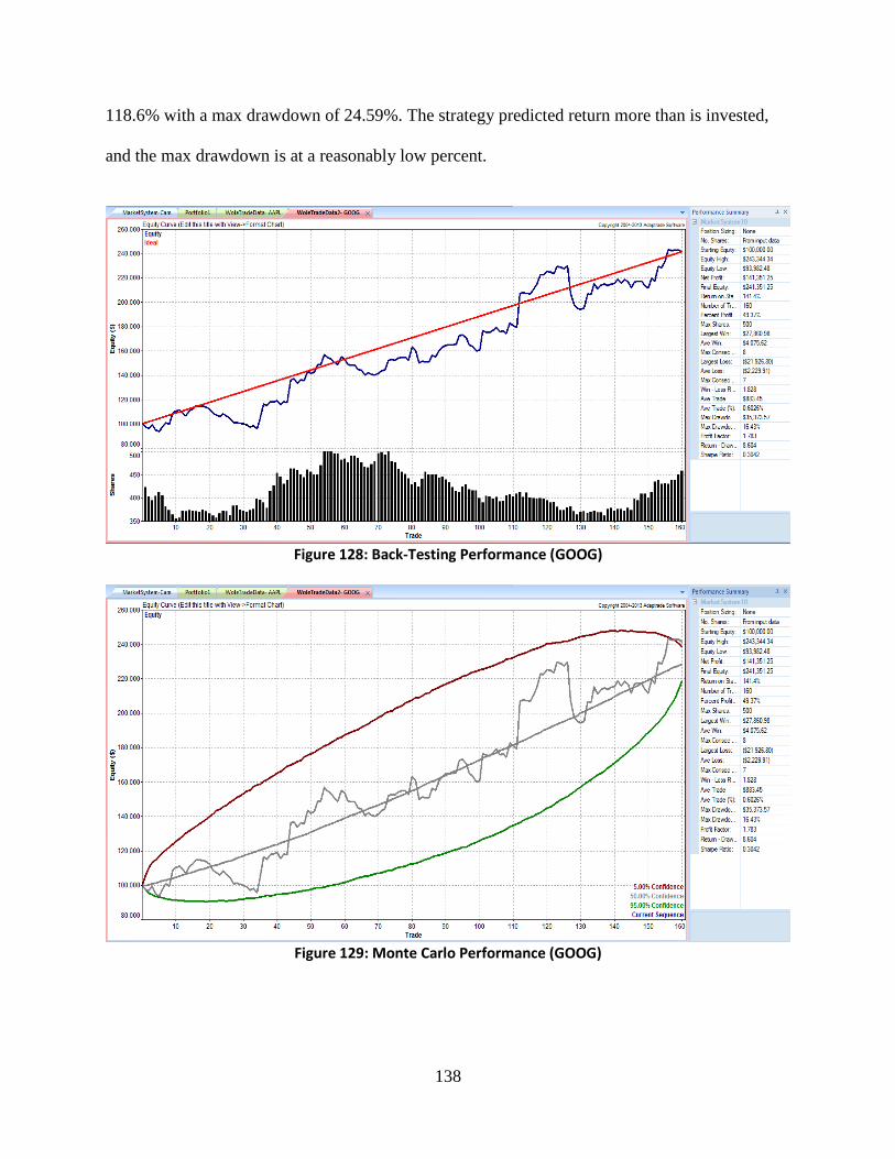
138
118.6% with a max drawdown of 24.59%. The strategy predicted return more than is invested,
and the max drawdown is at a reasonably low percent.
Figure 128: Back-Testing Performance (GOOG)
Figure 129: Monte Carlo Performance (GOOG)
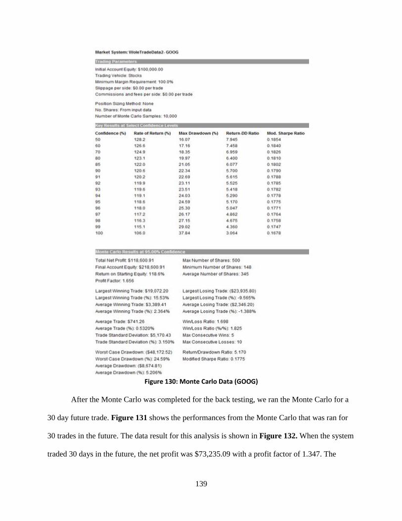
139
Figure 130: Monte Carlo Data (GOOG)
After the Monte Carlo was completed for the back testing, we ran the Monte Carlo for a
30 day future trade. Figure 131 shows the performances from the Monte Carlo that was ran for
30 trades in the future. The data result for this analysis is shown in Figure 132. When the system
traded 30 days in the future, the net profit was $73,235.09 with a profit factor of 1.347. The
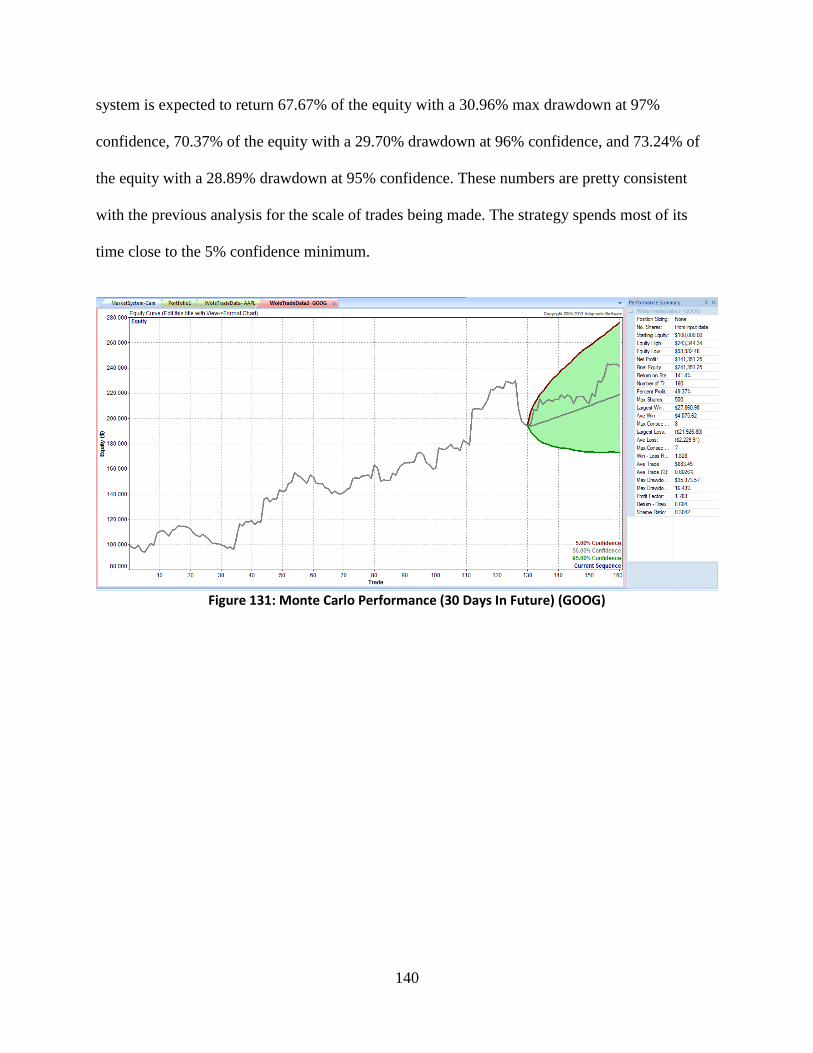
140
system is expected to return 67.67% of the equity with a 30.96% max drawdown at 97%
confidence, 70.37% of the equity with a 29.70% drawdown at 96% confidence, and 73.24% of
the equity with a 28.89% drawdown at 95% confidence. These numbers are pretty consistent
with the previous analysis for the scale of trades being made. The strategy spends most of its
time close to the 5% confidence minimum.
Figure 131: Monte Carlo Performance (30 Days In Future) (GOOG)
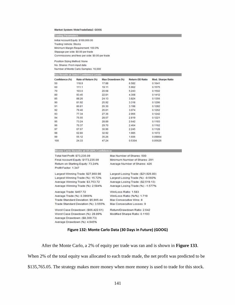
141
Figure 132: Monte Carlo Data (30 Days in Future) (GOOG)
After the Monte Carlo, a 2% of equity per trade was ran and is shown in Figure 133.
When 2% of the total equity was allocated to each trade made, the net profit was predicted to be
$135,765.05. The strategy makes more money when more money is used to trade for this stock.
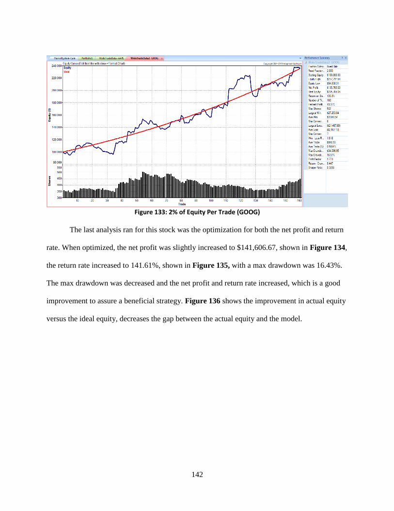
142
Figure 133: 2% of Equity Per Trade (GOOG)
The last analysis ran for this stock was the optimization for both the net profit and return
rate. When optimized, the net profit was slightly increased to $141,606.67, shown in Figure 134,
the return rate increased to 141.61%, shown in Figure 135, with a max drawdown was 16.43%.
The max drawdown was decreased and the net profit and return rate increased, which is a good
improvement to assure a beneficial strategy. Figure 136 shows the improvement in actual equity
versus the ideal equity, decreases the gap between the actual equity and the model.
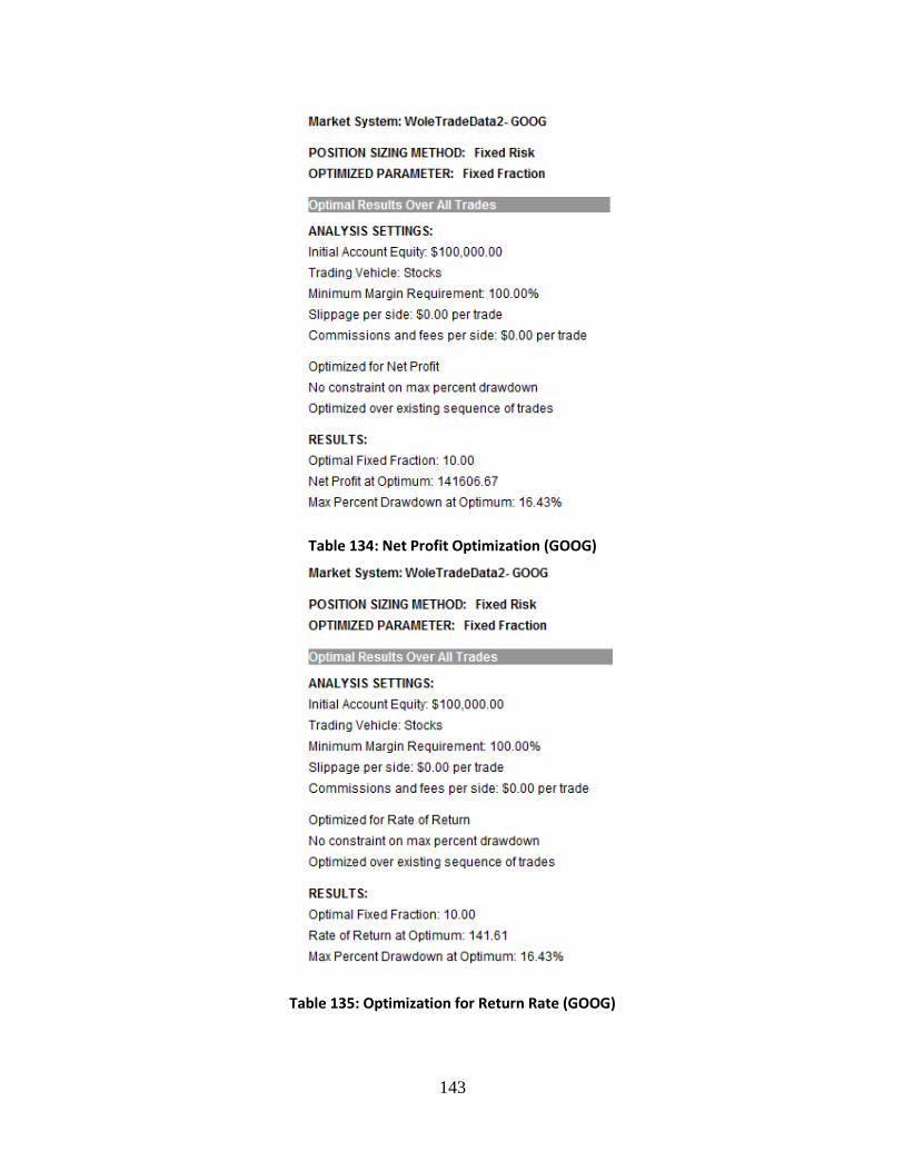
143
Table 134: Net Profit Optimization (GOOG)
Table 135: Optimization for Return Rate (GOOG)
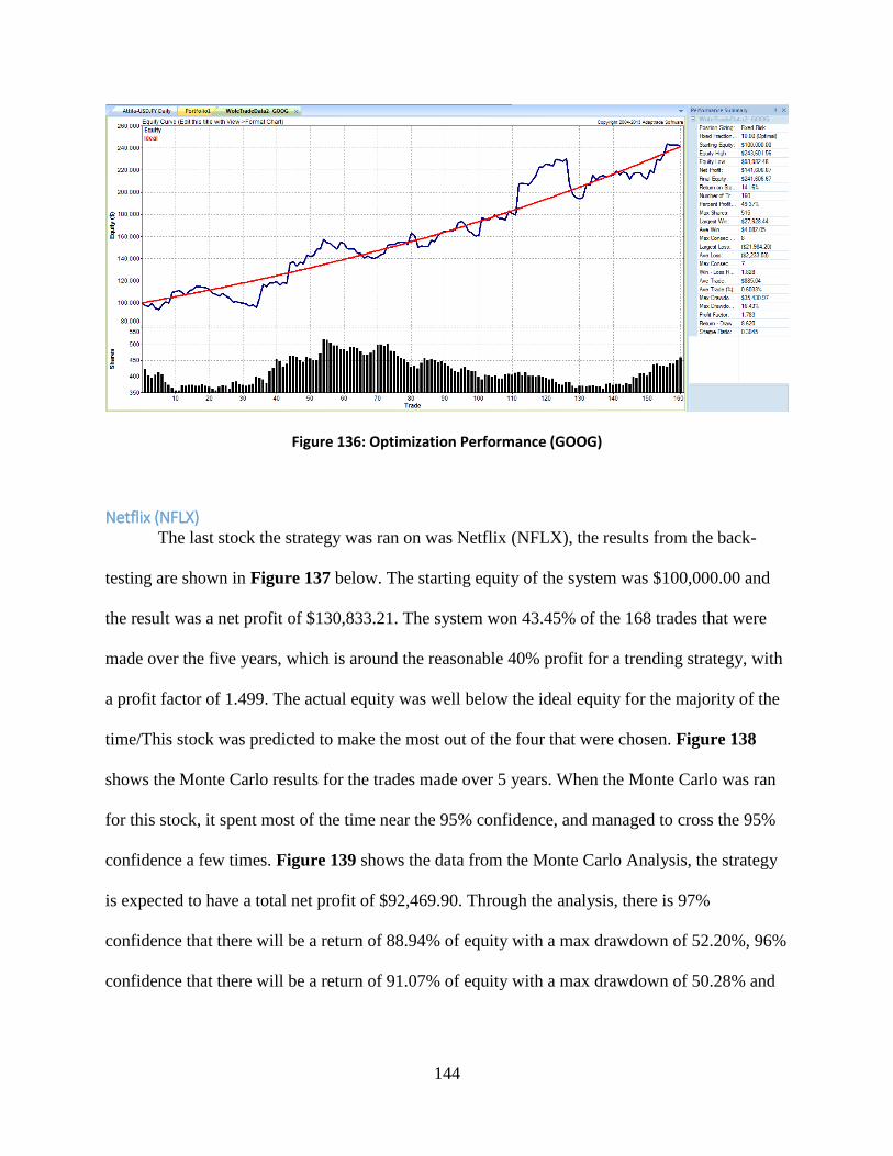
144
Figure 136: Optimization Performance (GOOG)
Netflix (NFLX) The last stock the strategy was ran on was Netflix (NFLX), the results from the back-
testing are shown in Figure 137 below. The starting equity of the system was $100,000.00 and
the result was a net profit of $130,833.21. The system won 43.45% of the 168 trades that were
made over the five years, which is around the reasonable 40% profit for a trending strategy, with
a profit factor of 1.499. The actual equity was well below the ideal equity for the majority of the
time/This stock was predicted to make the most out of the four that were chosen. Figure 138
shows the Monte Carlo results for the trades made over 5 years. When the Monte Carlo was ran
for this stock, it spent most of the time near the 95% confidence, and managed to cross the 95%
confidence a few times. Figure 139 shows the data from the Monte Carlo Analysis, the strategy
is expected to have a total net profit of $92,469.90. Through the analysis, there is 97%
confidence that there will be a return of 88.94% of equity with a max drawdown of 52.20%, 96%
confidence that there will be a return of 91.07% of equity with a max drawdown of 50.28% and
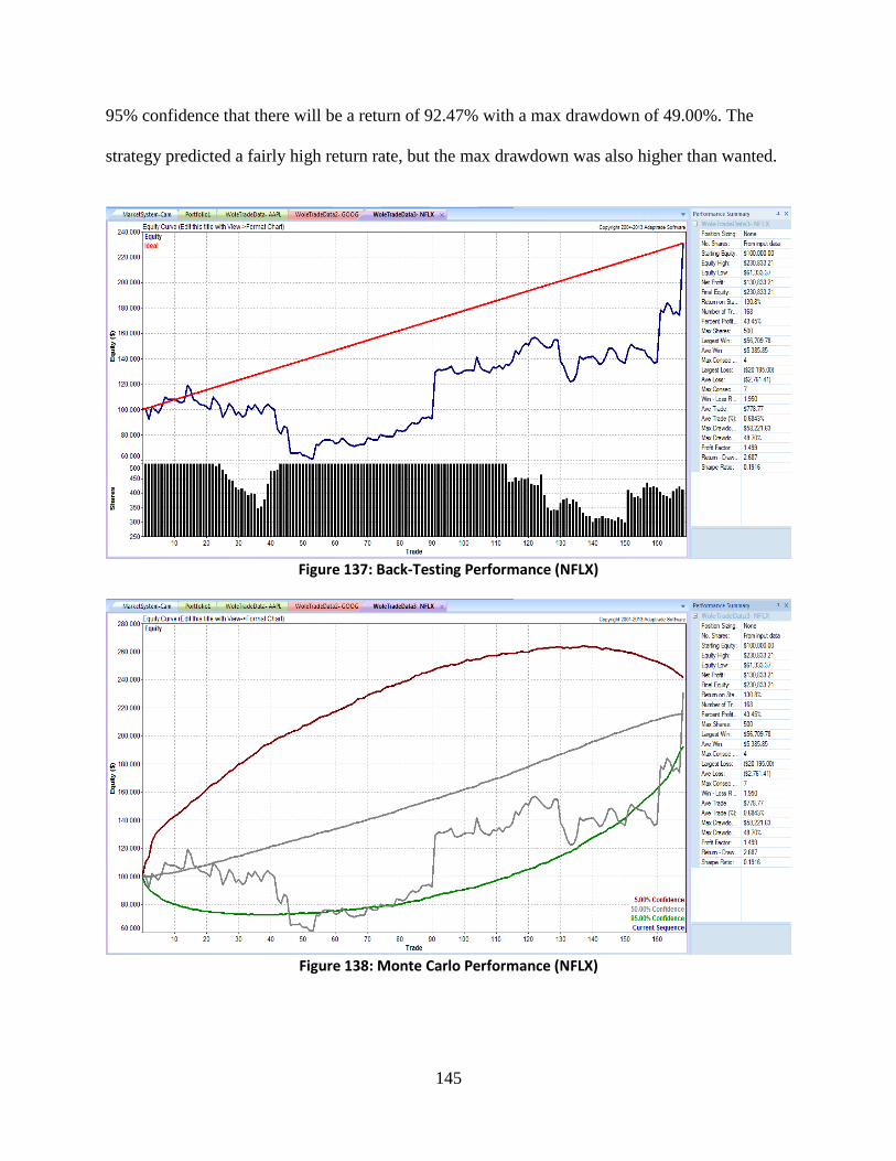
145
95% confidence that there will be a return of 92.47% with a max drawdown of 49.00%. The
strategy predicted a fairly high return rate, but the max drawdown was also higher than wanted.
Figure 137: Back-Testing Performance (NFLX)
Figure 138: Monte Carlo Performance (NFLX)
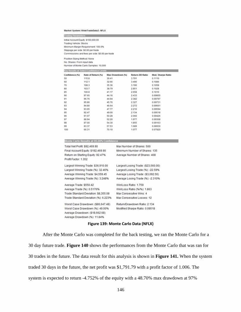
146
Figure 139: Monte Carlo Data (NFLX)
After the Monte Carlo was completed for the back testing, we ran the Monte Carlo for a
30 day future trade. Figure 140 shows the performances from the Monte Carlo that was ran for
30 trades in the future. The data result for this analysis is shown in Figure 141. When the system
traded 30 days in the future, the net profit was $1,791.79 with a profit factor of 1.006. The
system is expected to return -4.752% of the equity with a 48.70% max drawdown at 97%
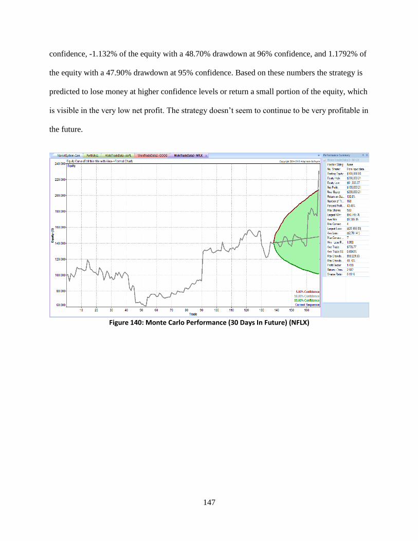
147
confidence, -1.132% of the equity with a 48.70% drawdown at 96% confidence, and 1.1792% of
the equity with a 47.90% drawdown at 95% confidence. Based on these numbers the strategy is
predicted to lose money at higher confidence levels or return a small portion of the equity, which
is visible in the very low net profit. The strategy doesn’t seem to continue to be very profitable in
the future.
Figure 140: Monte Carlo Performance (30 Days In Future) (NFLX)
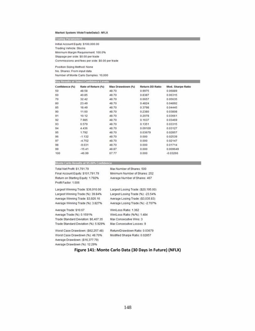
148
Figure 141: Monte Carlo Data (30 Days in Future) (NFLX)
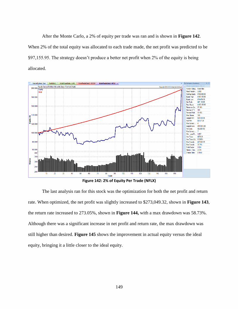
149
After the Monte Carlo, a 2% of equity per trade was ran and is shown in Figure 142.
When 2% of the total equity was allocated to each trade made, the net profit was predicted to be
$97,155.95. The strategy doesn’t produce a better net profit when 2% of the equity is being
allocated.
Figure 142: 2% of Equity Per Trade (NFLX)
The last analysis ran for this stock was the optimization for both the net profit and return
rate. When optimized, the net profit was slightly increased to $273,049.32, shown in Figure 143,
the return rate increased to 273.05%, shown in Figure 144, with a max drawdown was 58.73%.
Although there was a significant increase in net profit and return rate, the max drawdown was
still higher than desired. Figure 145 shows the improvement in actual equity versus the ideal
equity, bringing it a little closer to the ideal equity.
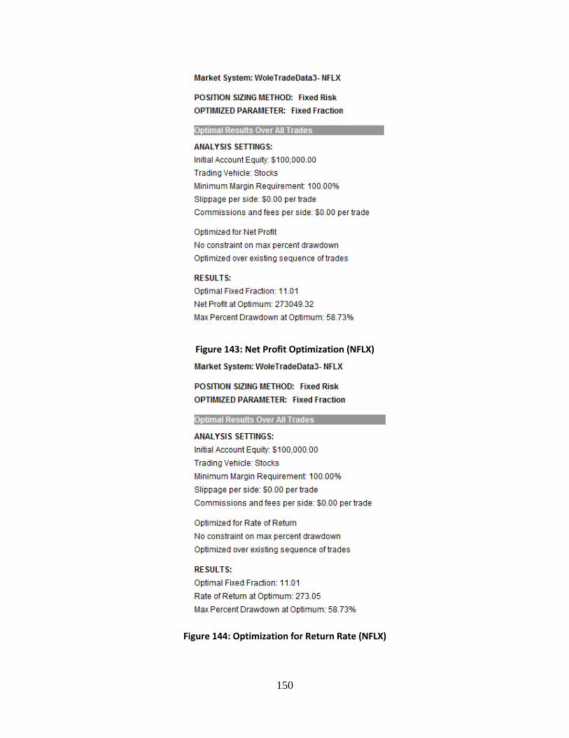
150
Figure 143: Net Profit Optimization (NFLX)
Figure 144: Optimization for Return Rate (NFLX)
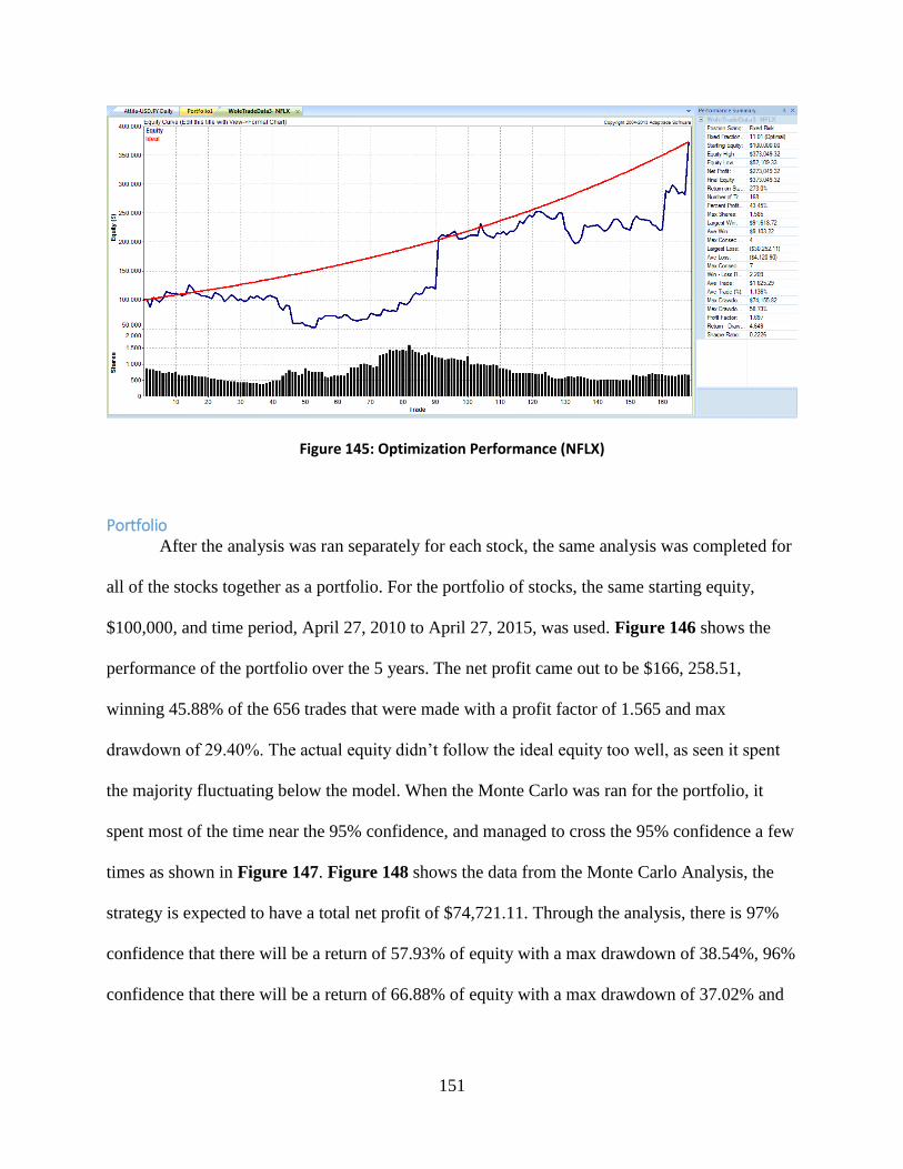
151
Figure 145: Optimization Performance (NFLX)
Portfolio After the analysis was ran separately for each stock, the same analysis was completed for
all of the stocks together as a portfolio. For the portfolio of stocks, the same starting equity,
$100,000, and time period, April 27, 2010 to April 27, 2015, was used. Figure 146 shows the
performance of the portfolio over the 5 years. The net profit came out to be $166, 258.51,
winning 45.88% of the 656 trades that were made with a profit factor of 1.565 and max
drawdown of 29.40%. The actual equity didn’t follow the ideal equity too well, as seen it spent
the majority fluctuating below the model. When the Monte Carlo was ran for the portfolio, it
spent most of the time near the 95% confidence, and managed to cross the 95% confidence a few
times as shown in Figure 147. Figure 148 shows the data from the Monte Carlo Analysis, the
strategy is expected to have a total net profit of $74,721.11. Through the analysis, there is 97%
confidence that there will be a return of 57.93% of equity with a max drawdown of 38.54%, 96%
confidence that there will be a return of 66.88% of equity with a max drawdown of 37.02% and
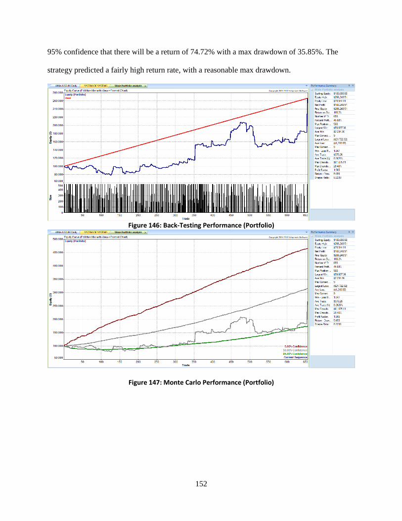
152
95% confidence that there will be a return of 74.72% with a max drawdown of 35.85%. The
strategy predicted a fairly high return rate, with a reasonable max drawdown.
Figure 146: Back-Testing Performance (Portfolio)
Figure 147: Monte Carlo Performance (Portfolio)
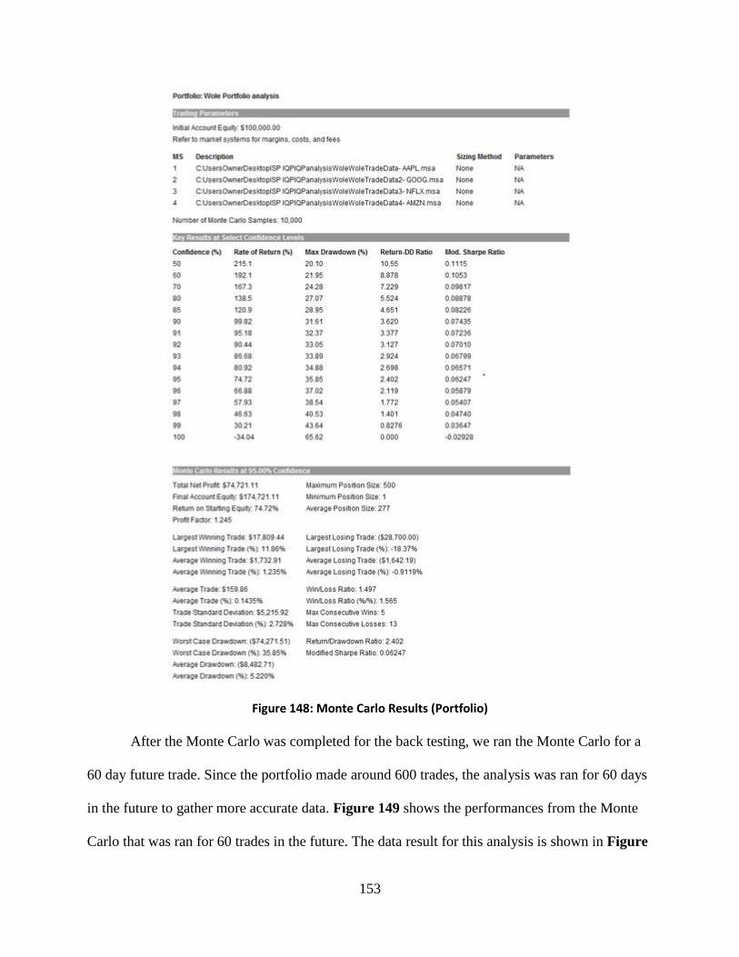
153
Figure 148: Monte Carlo Results (Portfolio)
After the Monte Carlo was completed for the back testing, we ran the Monte Carlo for a
60 day future trade. Since the portfolio made around 600 trades, the analysis was ran for 60 days
in the future to gather more accurate data. Figure 149 shows the performances from the Monte
Carlo that was ran for 60 trades in the future. The data result for this analysis is shown in Figure
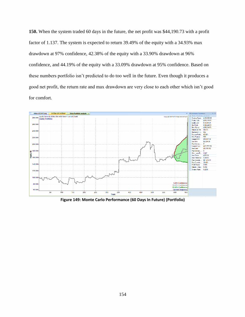
154
150. When the system traded 60 days in the future, the net profit was $44,190.73 with a profit
factor of 1.137. The system is expected to return 39.49% of the equity with a 34.93% max
drawdown at 97% confidence, 42.38% of the equity with a 33.90% drawdown at 96%
confidence, and 44.19% of the equity with a 33.09% drawdown at 95% confidence. Based on
these numbers portfolio isn’t predicted to do too well in the future. Even though it produces a
good net profit, the return rate and max drawdown are very close to each other which isn’t good
for comfort.
Figure 149: Monte Carlo Performance (60 Days In Future) (Portfolio)
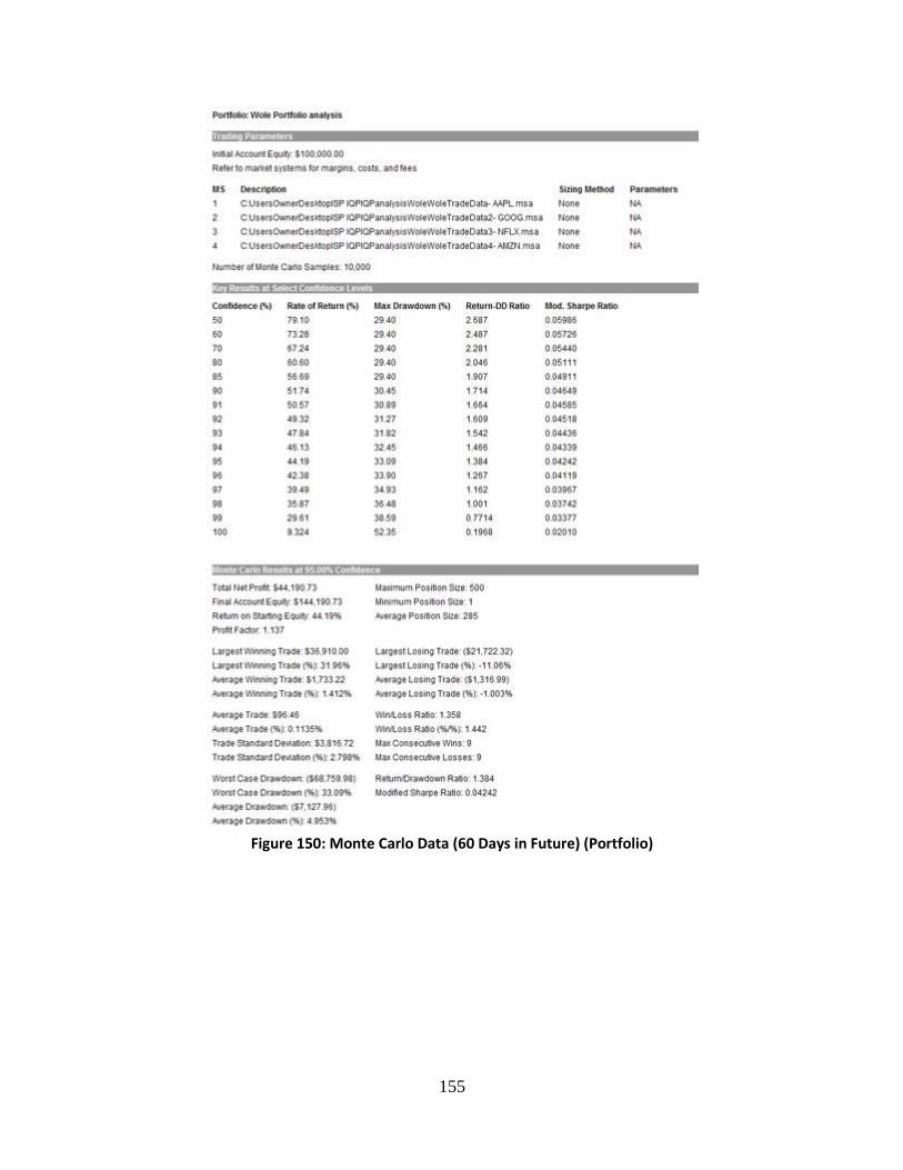
155
Figure 150: Monte Carlo Data (60 Days in Future) (Portfolio)
156
The last analysis ran for this stock was the optimization for both the net profit and return
rate. When optimized, the net profit was slightly increased to $834,913.7, shown in Figure 151,
the return rate increased to 834.91%, shown in Figure 152, with a max drawdown was 36.43%.
When the net profit was optimize, Amazon (AMZN) got 20.01% of the equity, Netflix (NFLX)
got 11.01% of the equity, Apple (APPL) got 10% of the equity and Google (GOOG) got 0% of
the equity. This shows that Amazon (AMZN) performed the best in the portfolio, while Apple
(AAPL) and Netflix (NFLX) were fairly equal. Unfortunately, Google (GOOG) did the worst out
of the four stocks and didn’t receive any percent of the equity. When the return rate was
optimized, Netflix (NFLX) got 21.01% of the equity, Apple (AAPL) got 20% of the equity,
Amazon (AMZN) got 10.01% of the equity and Google (GOOG) got 0% of the equity. This
shows that Apple (AAPL) and Netflix (NFLX) performed the best, both receive fairly equal
amount of the equity. Amazon (AMZN) didn’t do as well when the return rate was optimized,
but still received a decent percent of the equity. Unfortunately, Google (GOOG) was the weakest
stock and failed to receive any portion of the equity. Figure 153 shows the improvement in
actual equity versus the ideal equity, bringing it a little tighter to the ideal equity.
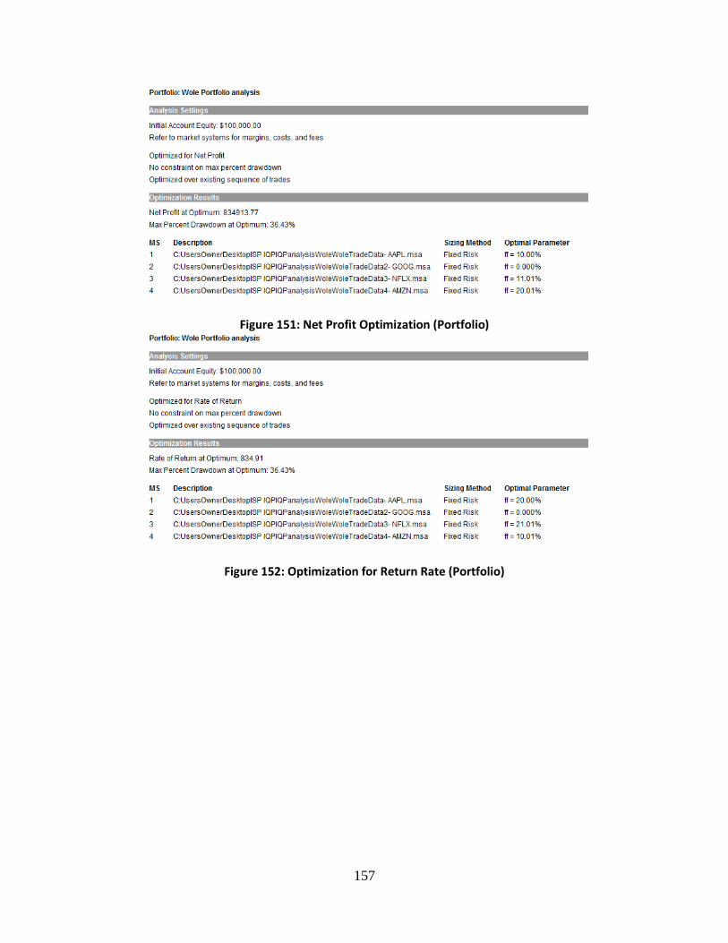
157
Figure 151: Net Profit Optimization (Portfolio)
Figure 152: Optimization for Return Rate (Portfolio)
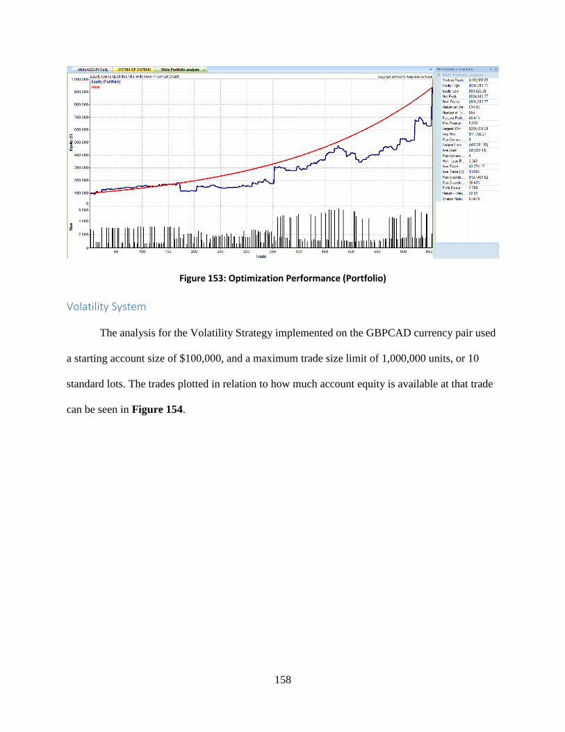
158
Figure 153: Optimization Performance (Portfolio)
Volatility System
The analysis for the Volatility Strategy implemented on the GBPCAD currency pair used
a starting account size of $100,000, and a maximum trade size limit of 1,000,000 units, or 10
standard lots. The trades plotted in relation to how much account equity is available at that trade
can be seen in Figure 154.
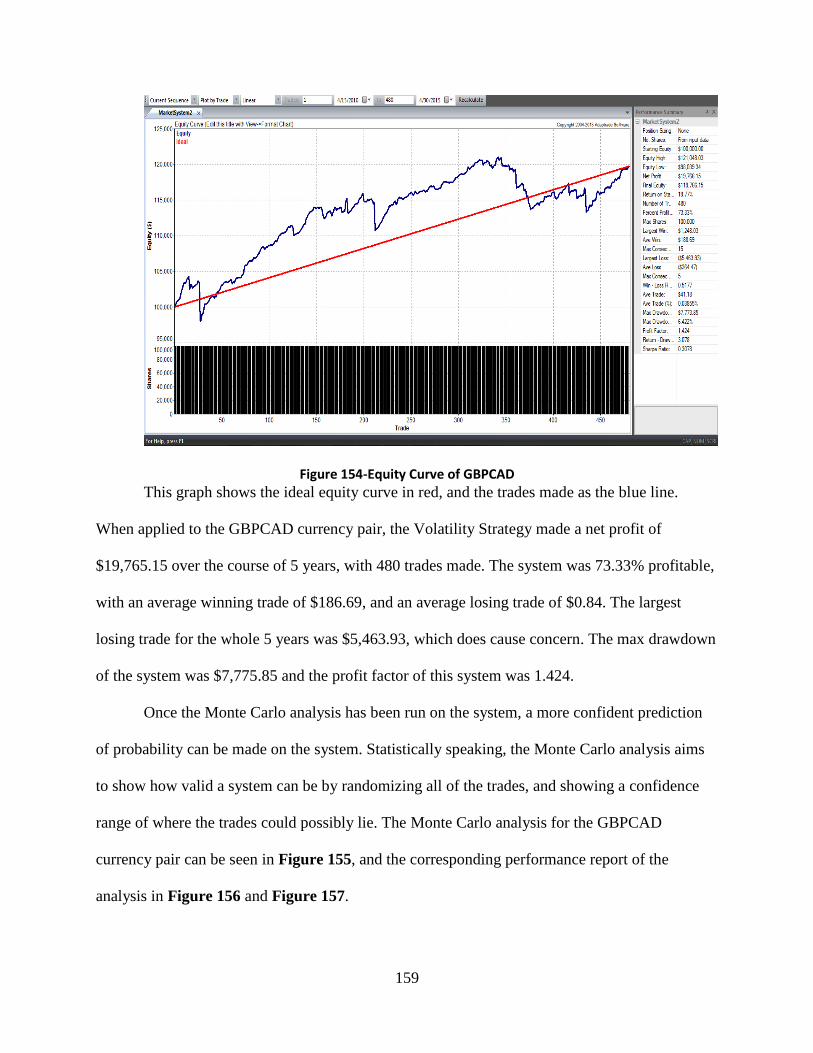
159
Figure 154-Equity Curve of GBPCAD
This graph shows the ideal equity curve in red, and the trades made as the blue line.
When applied to the GBPCAD currency pair, the Volatility Strategy made a net profit of
$19,765.15 over the course of 5 years, with 480 trades made. The system was 73.33% profitable,
with an average winning trade of $186.69, and an average losing trade of $0.84. The largest
losing trade for the whole 5 years was $5,463.93, which does cause concern. The max drawdown
of the system was $7,775.85 and the profit factor of this system was 1.424.
Once the Monte Carlo analysis has been run on the system, a more confident prediction
of probability can be made on the system. Statistically speaking, the Monte Carlo analysis aims
to show how valid a system can be by randomizing all of the trades, and showing a confidence
range of where the trades could possibly lie. The Monte Carlo analysis for the GBPCAD
currency pair can be seen in Figure 155, and the corresponding performance report of the
analysis in Figure 156 and Figure 157.
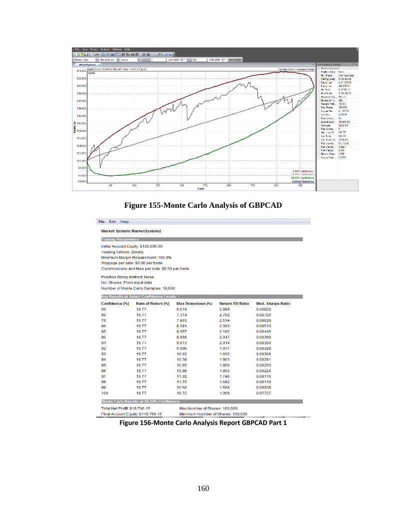
160
Figure 155-Monte Carlo Analysis of GBPCAD
Figure 156-Monte Carlo Analysis Report GBPCAD Part 1
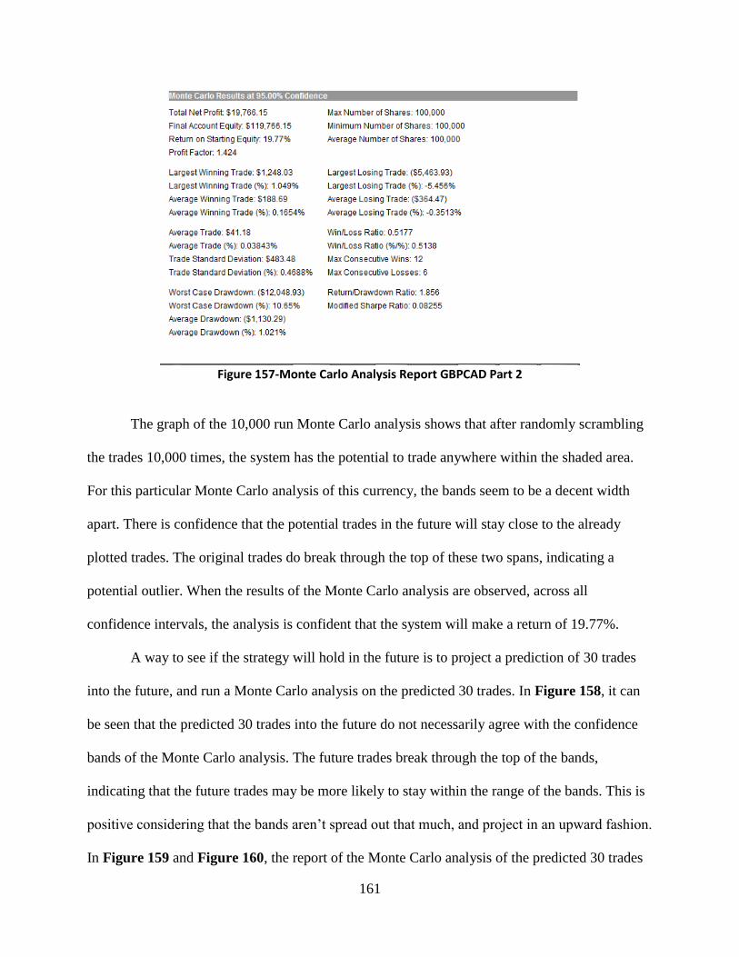
161
Figure 157-Monte Carlo Analysis Report GBPCAD Part 2
The graph of the 10,000 run Monte Carlo analysis shows that after randomly scrambling
the trades 10,000 times, the system has the potential to trade anywhere within the shaded area.
For this particular Monte Carlo analysis of this currency, the bands seem to be a decent width
apart. There is confidence that the potential trades in the future will stay close to the already
plotted trades. The original trades do break through the top of these two spans, indicating a
potential outlier. When the results of the Monte Carlo analysis are observed, across all
confidence intervals, the analysis is confident that the system will make a return of 19.77%.
A way to see if the strategy will hold in the future is to project a prediction of 30 trades
into the future, and run a Monte Carlo analysis on the predicted 30 trades. In Figure 158, it can
be seen that the predicted 30 trades into the future do not necessarily agree with the confidence
bands of the Monte Carlo analysis. The future trades break through the top of the bands,
indicating that the future trades may be more likely to stay within the range of the bands. This is
positive considering that the bands aren’t spread out that much, and project in an upward fashion.
In Figure 159 and Figure 160, the report of the Monte Carlo analysis of the predicted 30 trades
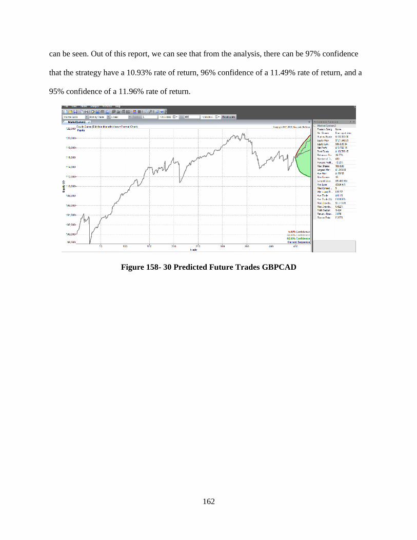
162
can be seen. Out of this report, we can see that from the analysis, there can be 97% confidence
that the strategy have a 10.93% rate of return, 96% confidence of a 11.49% rate of return, and a
95% confidence of a 11.96% rate of return.
Figure 158- 30 Predicted Future Trades GBPCAD
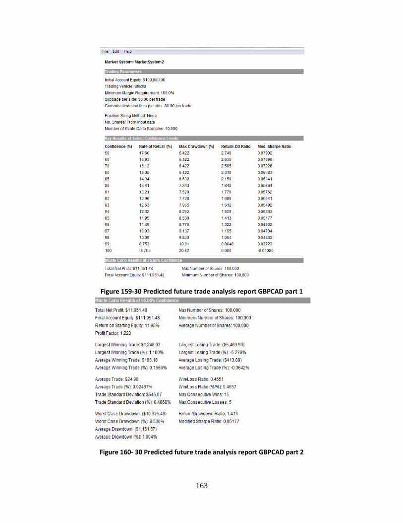
163
Figure 159-30 Predicted future trade analysis report GBPCAD part 1
Figure 160- 30 Predicted future trade analysis report GBPCAD part 2
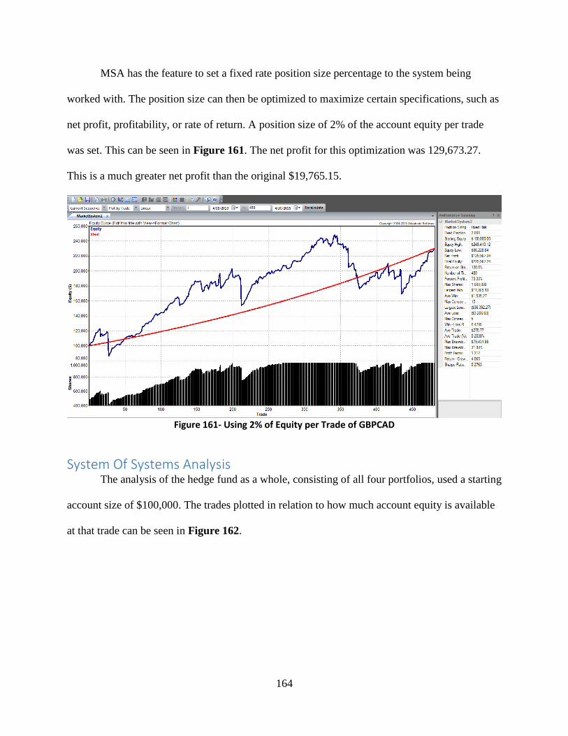
164
MSA has the feature to set a fixed rate position size percentage to the system being
worked with. The position size can then be optimized to maximize certain specifications, such as
net profit, profitability, or rate of return. A position size of 2% of the account equity per trade
was set. This can be seen in Figure 161. The net profit for this optimization was 129,673.27.
This is a much greater net profit than the original $19,765.15.
Figure 161- Using 2% of Equity per Trade of GBPCAD
System Of Systems Analysis The analysis of the hedge fund as a whole, consisting of all four portfolios, used a starting
account size of $100,000. The trades plotted in relation to how much account equity is available
at that trade can be seen in Figure 162.
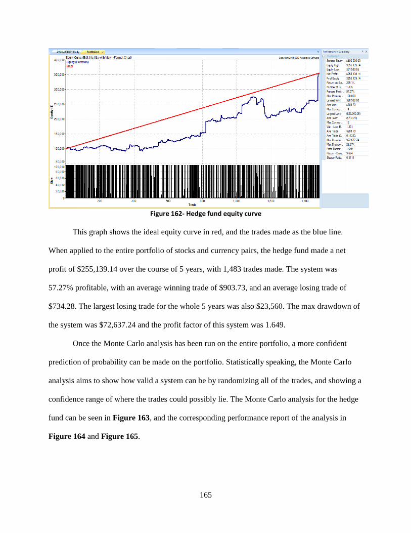
165
Figure 162- Hedge fund equity curve
This graph shows the ideal equity curve in red, and the trades made as the blue line.
When applied to the entire portfolio of stocks and currency pairs, the hedge fund made a net
profit of $255,139.14 over the course of 5 years, with 1,483 trades made. The system was
57.27% profitable, with an average winning trade of $903.73, and an average losing trade of
$734.28. The largest losing trade for the whole 5 years was also $23,560. The max drawdown of
the system was $72,637.24 and the profit factor of this system was 1.649.
Once the Monte Carlo analysis has been run on the entire portfolio, a more confident
prediction of probability can be made on the portfolio. Statistically speaking, the Monte Carlo
analysis aims to show how valid a system can be by randomizing all of the trades, and showing a
confidence range of where the trades could possibly lie. The Monte Carlo analysis for the hedge
fund can be seen in Figure 163, and the corresponding performance report of the analysis in
Figure 164 and Figure 165.
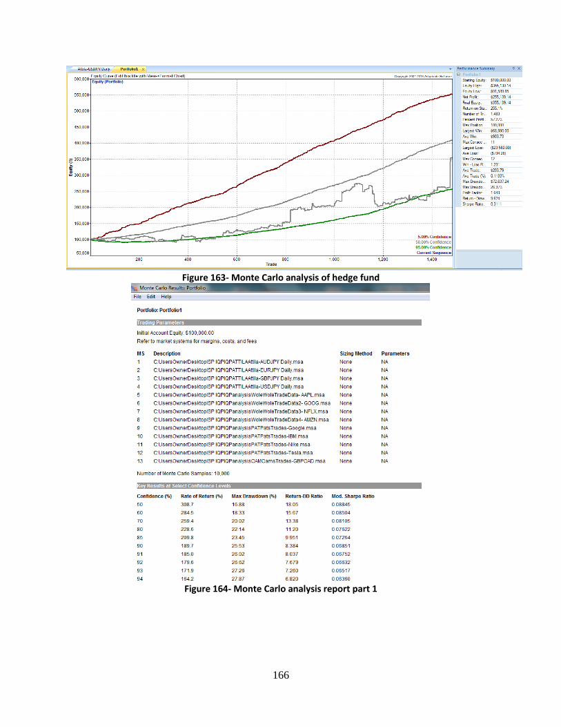
166
Figure 163- Monte Carlo analysis of hedge fund
Figure 164- Monte Carlo analysis report part 1
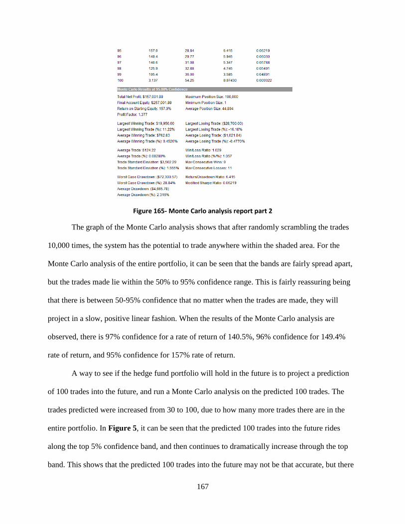
167
Figure 165- Monte Carlo analysis report part 2
The graph of the Monte Carlo analysis shows that after randomly scrambling the trades
10,000 times, the system has the potential to trade anywhere within the shaded area. For the
Monte Carlo analysis of the entire portfolio, it can be seen that the bands are fairly spread apart,
but the trades made lie within the 50% to 95% confidence range. This is fairly reassuring being
that there is between 50-95% confidence that no matter when the trades are made, they will
project in a slow, positive linear fashion. When the results of the Monte Carlo analysis are
observed, there is 97% confidence for a rate of return of 140.5%, 96% confidence for 149.4%
rate of return, and 95% confidence for 157% rate of return.
A way to see if the hedge fund portfolio will hold in the future is to project a prediction
of 100 trades into the future, and run a Monte Carlo analysis on the predicted 100 trades. The
trades predicted were increased from 30 to 100, due to how many more trades there are in the
entire portfolio. In Figure 5, it can be seen that the predicted 100 trades into the future rides
along the top 5% confidence band, and then continues to dramatically increase through the top
band. This shows that the predicted 100 trades into the future may not be that accurate, but there
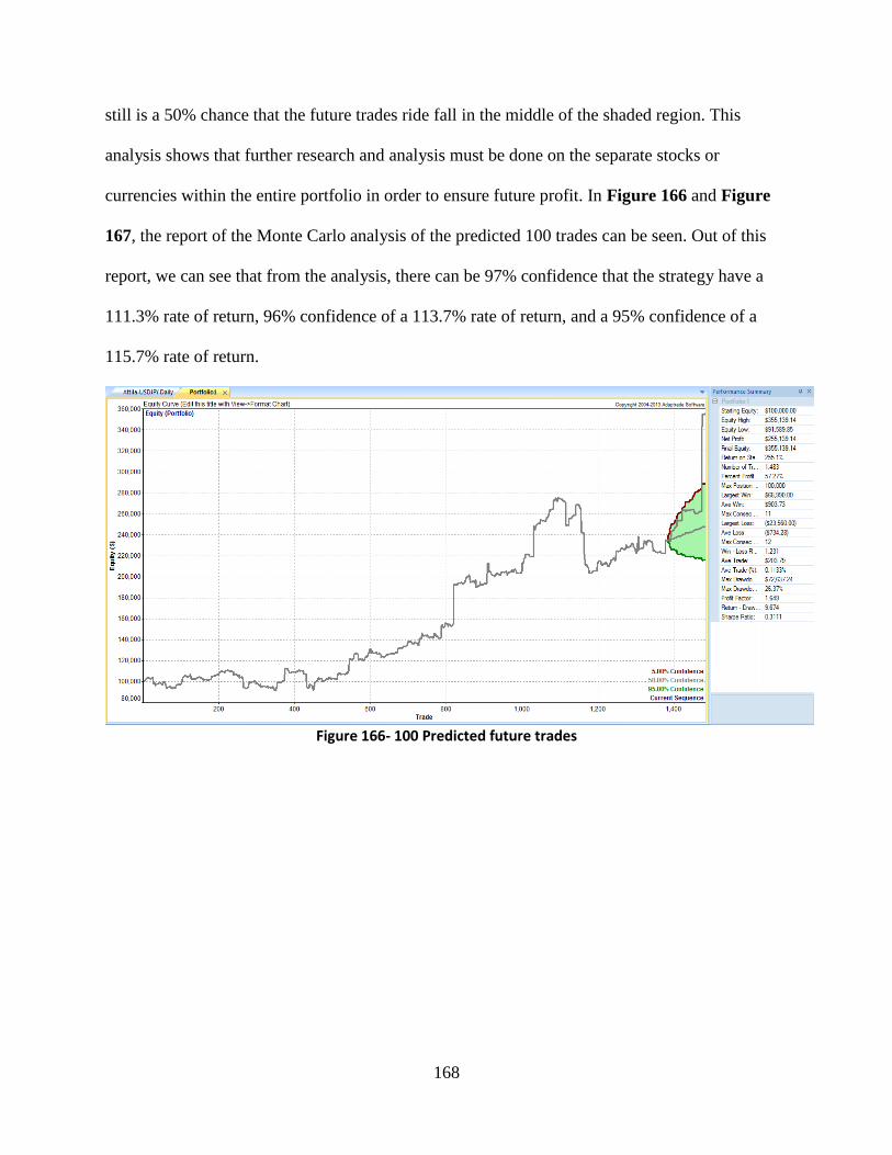
168
still is a 50% chance that the future trades ride fall in the middle of the shaded region. This
analysis shows that further research and analysis must be done on the separate stocks or
currencies within the entire portfolio in order to ensure future profit. In Figure 166 and Figure
167, the report of the Monte Carlo analysis of the predicted 100 trades can be seen. Out of this
report, we can see that from the analysis, there can be 97% confidence that the strategy have a
111.3% rate of return, 96% confidence of a 113.7% rate of return, and a 95% confidence of a
115.7% rate of return.
Figure 166- 100 Predicted future trades
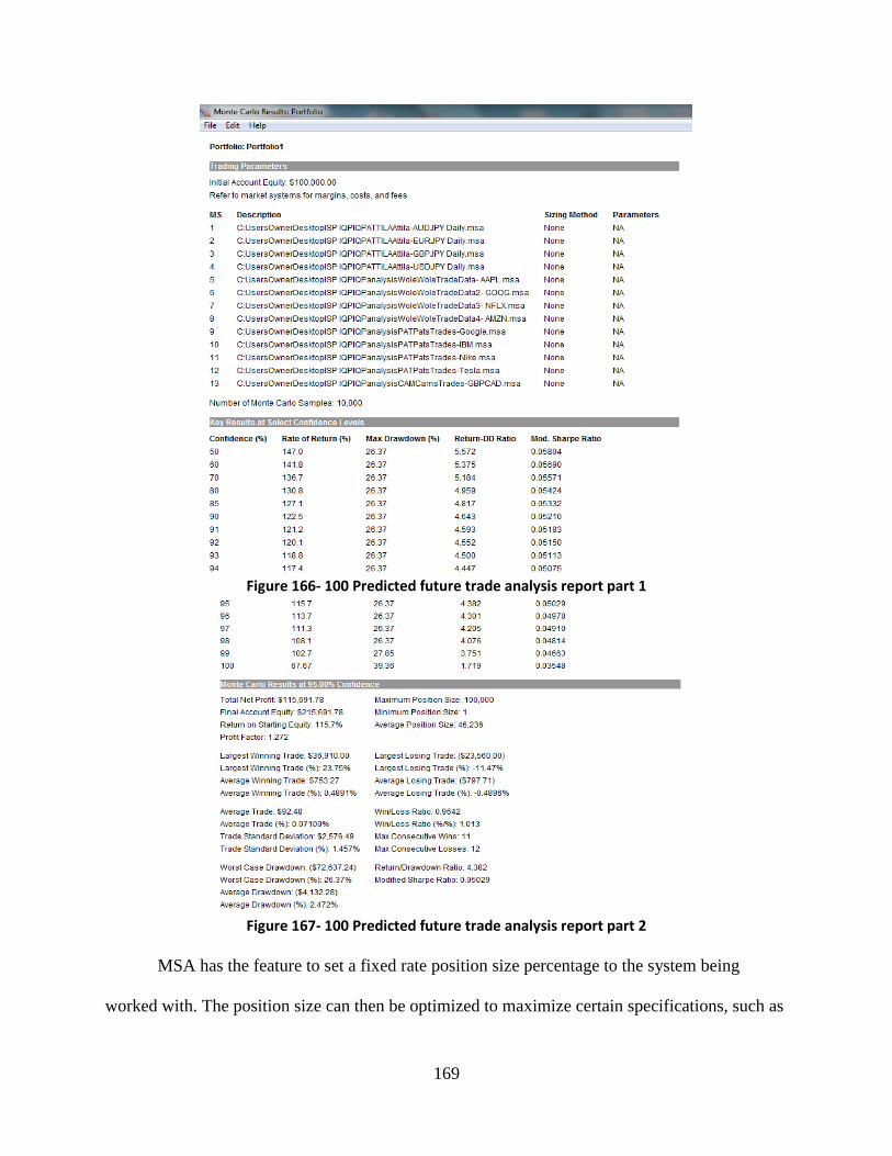
169
Figure 166- 100 Predicted future trade analysis report part 1
Figure 167- 100 Predicted future trade analysis report part 2
MSA has the feature to set a fixed rate position size percentage to the system being
worked with. The position size can then be optimized to maximize certain specifications, such as
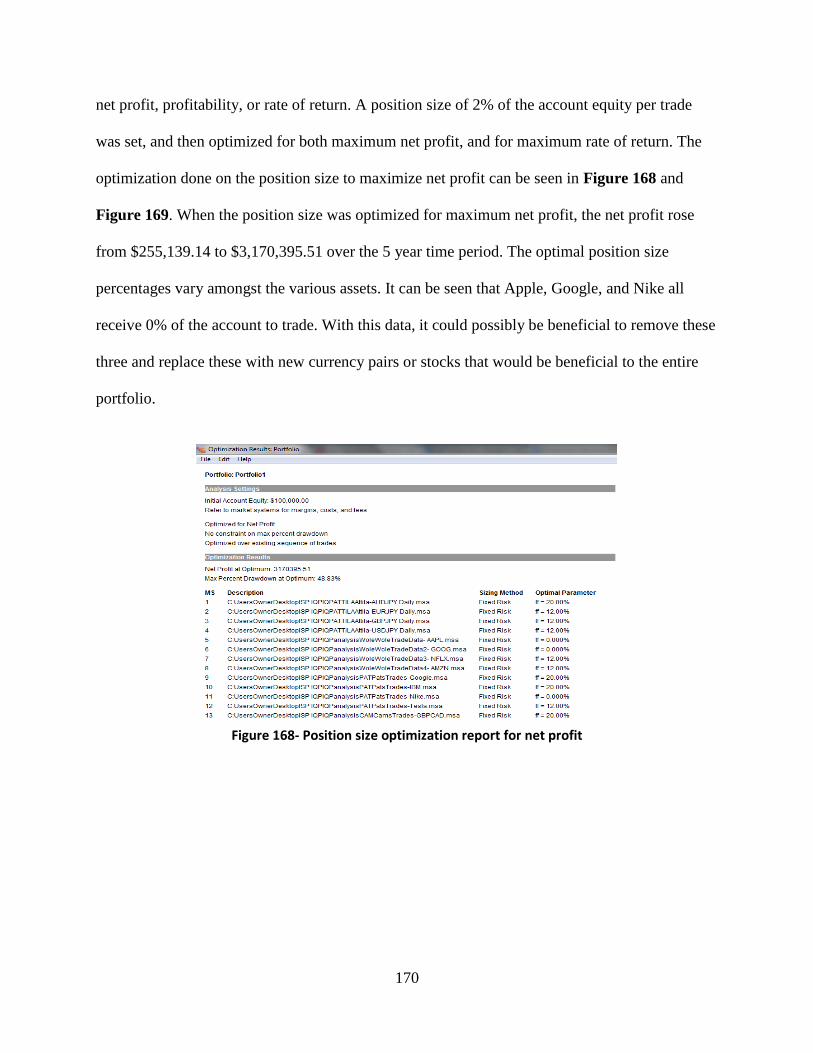
170
net profit, profitability, or rate of return. A position size of 2% of the account equity per trade
was set, and then optimized for both maximum net profit, and for maximum rate of return. The
optimization done on the position size to maximize net profit can be seen in Figure 168 and
Figure 169. When the position size was optimized for maximum net profit, the net profit rose
from $255,139.14 to $3,170,395.51 over the 5 year time period. The optimal position size
percentages vary amongst the various assets. It can be seen that Apple, Google, and Nike all
receive 0% of the account to trade. With this data, it could possibly be beneficial to remove these
three and replace these with new currency pairs or stocks that would be beneficial to the entire
portfolio.
Figure 168- Position size optimization report for net profit
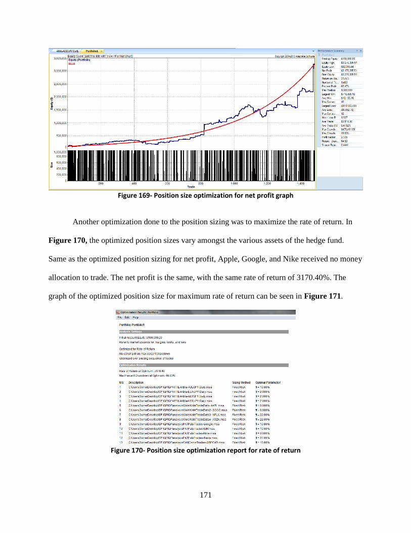
171
Figure 169- Position size optimization for net profit graph
Another optimization done to the position sizing was to maximize the rate of return. In
Figure 170, the optimized position sizes vary amongst the various assets of the hedge fund.
Same as the optimized position sizing for net profit, Apple, Google, and Nike received no money
allocation to trade. The net profit is the same, with the same rate of return of 3170.40%. The
graph of the optimized position size for maximum rate of return can be seen in Figure 171.
Figure 170- Position size optimization report for rate of return
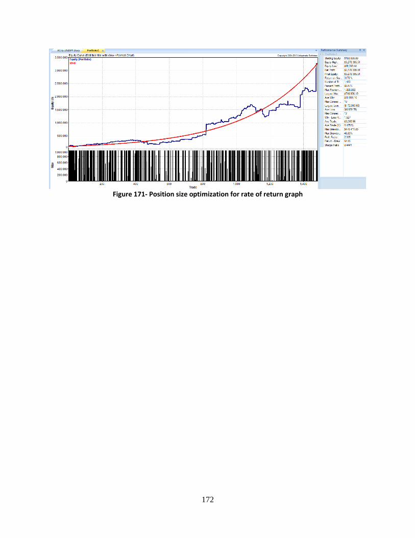
172
Figure 171- Position size optimization for rate of return graph
173
Conclusion
Adaptive Moving Average System This automated system was profitable for each stock tested upon in back testing, yet with
further future analysis it seems that the strategy worked much more efficiently for future use
with select stocks. As my optimal portfolio suggested, the parameters set for Nike stock were
indeed the most efficient. In order to trade real money, some small alterations would be made to
the strategy, but this stock would be a top choice for the AMA strategy. Some parameters that
could be changed are the span values of both moving average indicators as they were once
optimized in Tradestation; they may have been over fit to historical data. Also, stop values and
profit targets could be analyzed again and changed to increase the efficiency of the system. The
daily charts are a great fit for this strategy, but the system could also be used on weekly bar
charts where success has previously been recorded. The system is currently usable in the stock
market yet more tests can be ran to make a more profitable and comfortable automated strategy.
Ichimoku Trading System Considering the profit factor, and that the entire portfolio for the "Ichi" strategy was over
50% profitable, this strategy could potentially be ready to use in a live market. One "catch" to
this strategy is that it is tailored for markets that are in an overall up-trend, so the market would
have to be chosen accordingly. The risk is managed exceptionally well, with a max drawdown of
$6.72, which can be very comforting to many people, especially considering that the starting
account size for that drawdown is $100,000. One thing that could potentially be changed for the
strategy is the size of the stop loss and the dollar trailing. Increasing these values can cause the
time stayed in the market to increase, but could potentially increase the max drawdown and the
174
average loss of a trade. More analysis would need to be done to see if this concept would work
better than the original.
Trend Following Turtle System The modified trend following system that was developed for this hedge fund satisfied the
objectives for the most part. The strategy made a lot of trades throughout the five years, which is
typically unusually for a trend following system, but is what was desired for this specific
strategy. The strategy won about 40% of the total trades that were made for each stock, which is
good for a trend following system. The system was able to catch the big jumps in the market and
did a fairly decent job of avoiding the noise, although the profit was still affected by it. One
negative was the drawdown was higher than sought compared to the return rate for some of the
stocks. Possible improvements that can be made would be implementing a stop loss to maximize
the profit. The system won a large amount of money, but the net profit was much lower due to
losing a large amount of money. With a stop loss implemented to minimize the largest lost and
lost on trades, the system would continue to make as much money as prior to the stop loss, but
wouldn’t be losing as much on trades. An indicator can also be implemented to improve the
filtering of noise. With these to improvements made, the strategy would be ready to begin
trading with real money.
Volatility Trading System The volatility automated trading system that was developed met most of the objectives,
but could be developed further for more success. The volatility system traded over 400 times for
the five-year plan and was still very profitable. When using 2% of equity per trade, the system is
even more profitable. This system could be ready for trading with real money, but it would have
to be monitored closely due to the big losers it sometimes encounters. Going forward with this
system, it would be smart to try and configure a stop loss of some sort to limit big losing trades.
175
The only problem encountered with this system was configuring the time filter, but once the
problem was solved no other problems were run into.
System Of Systems When the numbers are examined on the profitability of the hedge fund, there shows sign
of potentially being successful in the future. With a starting account size of $100,000, the entire
fund was able to make about 255%, $255,139, in a five year time span. Before optimization, the
average winning trade was $903.73, and the average loosing trade was $734.28. One aspect that
could potentially be alarming to some people is the max drawdown of the fund, which was
$72,637.24. In comparison to the amount made over the five years, this is a lot of money. Once
the entire fund was optimized for net profit, with a starting account size of $100,000, the hedge
fund made $3,170,395.51, with a profit factor of 2.335. The over all optimization ended up
removing 3 particular systems, the turtle traded Apple and Google, and the moving average
traded Nike. This shows that there is still some flaw to the hedge fund, and with more analysis,
these three systems can be changed to markets that are profitable. Considering vastly huge
difference between the beginning net profit and the optimized net profit, and taking into account
the 3 systems that were removed from trading, the hedge fund has the potential to make a much
larger profit. Aside from the small flaws, the entire system of systems that the hedge fund trades
is very profitable, and could potentially be used someday to trade live and with actual money.
176
Works Cited Investopedia Staff "Tutorial: Stock Basics Tutorial." Investopedia.Web. 01 Feb. 2015.
<http://www.investopedia.com/university/stocks/>
"Bond Markets & Prices." Bond Markets Defined. Web. 19 Feb. 2015.
<http://www.investinginbonds.com/marketataglance.asp?catid=31>
Radzicki, Michael J. "Introduction to Trading Systems and Devlopment." 2012. PowerPoint
Slides.
Chad Langager and Casey Murphy. “Dow Theory: Introduction.” Investopedia. Wed, 25 Feb
2015.
<http://www.investopedia.com/university/dowtheory/>
Investopedia Staff “Stock-Picking Strategies: CAN SLIM”.Investopedia.
<http://www.investopedia.com/university/stockpicking/stockpicking7.asp>
Justin Kuepper “Playing The Gap” Investopedia
<http://www.investopedia.com/articles/trading/05/playinggaps.asp>
Mishkin, F (2009). The Economics of Money, Banking, and Financial Markets, Ninth Edition.
Addison-Wesley Pg. 25-30, 147-162.
Wright, C (1998). Trading as a Business. Pg. 21-32
Currency Trader Staff. "Adaptive Moving Averages." Trading Strategies. Currency Trader, Aug.
2006. Web. May 2015.
<Dailyfx.com/forex>
Investopedia Staff. "Fundamental Analysis: Qualitative Factors - The Company." Investopedia.
Web. Apr. 2015.
<http://www.investopedia.com/university/fundamentalanalysis/fundanalysis2.asp>
Investopedia Staff. "Limit Order." Investopedia. Web. May 2015.
<http://www.investopedia.com/terms/l/limitorder.asp>
"Turtle Trading System - Wisdom Trading." Wisdom Trading. Web. 16 May 2015.
<http://www.wisdomtrading.com/trend-following/>
<http://www.wisdomtrading.com/public-trading-systems/turtle-trading-system/>
Raschke, Linda Bradford. "Volatility Breakout Systems." Traders Log RSS. Web. 16 May 2015.
<http://www.traderslog.com/volatility-breakout-systems/>
"Trendline Definition | Investopedia." Investopedia. 15 Mar. 2004. Web. 16 May 2015.
<http://www.investopedia.com/terms/t/trendline.asp>

177
"Moving Average (MA) Definition | Investopedia." Investopedia. 24 Nov. 2003. Web. 16 May
2015.
<http://www.investopedia.com/terms/m/movingaverage.asp>
Katz, Jeffrey Owen, and Donna L. McCormick. The Encyclopedia of Trading Strategies. New
York: McGraw-Hill, 2000. Print.
“Average True Range (ATR)” StockCharts.com. Web. 16 May 16, 2015
<http://stockcharts.com/school/doku.php?id=chart_school:technical_indicators:average_true_ran
ge_atr&gclid=CjwKEAjwpsGqBRCioKet--
bp_QcSJADCtbsb8RNk767hhc7TRulhzUtYLTnPDzv3ZRKSKUm4Pk_bWhoCcpTw_wcB>
"Ichimoku Clouds." StockCharts.com. Web. 16 May 2015.
<http://stockcharts.com/school/doku.php?id=chart_school:technical_indicators:ichimoku_cloud
&gclid=CjwKEAjwpsGqBRCioKet--
bp_QcSJADCtbsbLKElUO5jQzNZapqEDjWG89T7URtF1Qxat87sT_idchoCtK7w_wcB>

178
Appendices
Adaptive Moving Average Code
inputs: Price(close), EffRatioLength(10), FastAvgLength(4), SlowAvgLength(25), FastLength(2), SlowLength(50); variables: MAA(0), FastAvg(0), SlowAvg(0), LongConditionBar(0), LongCondition(False), CloseCondition(False); MAA = AdaptiveMovAvg(Price, EffRatioLength, FastAvgLength, SlowAvgLength ) ;
FastAvg = AverageFC( Price, FastLength); SlowAvg = AverageFC( Price, SlowLength);
LongCondition = FastAvg crosses above MAA;
If (LongCondition[3]) then begin
Buy ("LE") 500 shares next bar at market; LongCondition = False; end;
CloseCondition = FastAvg crosses below MAA;
If (CloseCondition[3]) then begin
Sell("close") 500 shares next bar at market; CloseCondition = False; end;
Begin
SetStopPosition; SetDollarTrailing(450); end;
Begin
SetStopPosition; Setpercenttrailing(1500,15); end;

179
Begin
Setstopposition; Setstoploss(500); end; Begin
SetStopPosition; SetProfitTarget(5000); end;
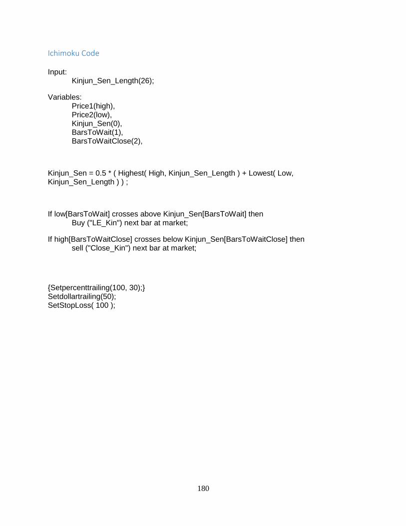
180
Ichimoku Code
Input: Kinjun_Sen_Length(26);
Variables: Price1(high), Price2(low), Kinjun_Sen(0), BarsToWait(1), BarsToWaitClose(2),
Kinjun_Sen = 0.5 * ( Highest( High, Kinjun_Sen_Length ) + Lowest( Low, Kinjun_Sen_Length ) ) ;
If low[BarsToWait] crosses above Kinjun_Sen[BarsToWait] then
Buy ("LE_Kin") next bar at market;
If high[BarsToWaitClose] crosses below Kinjun_Sen[BarsToWaitClose] then
sell ("Close_Kin") next bar at market;
{Setpercenttrailing(100, 30);}
Setdollartrailing(50); SetStopLoss( 100 );
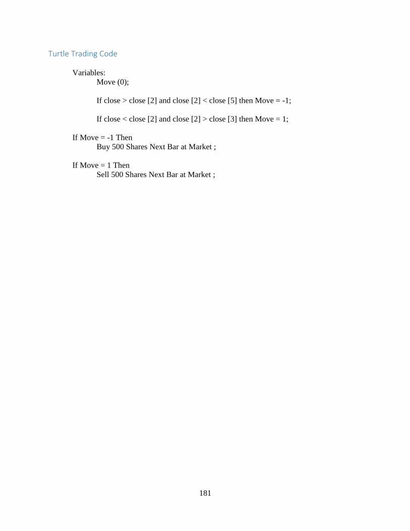
181
Turtle Trading Code
Variables:
Move (0);
If close > close [2] and close [2] < close [5] then Move = -1;
If close < close [2] and close [2] > close [3] then Move = 1;
If Move = -1 Then
Buy 500 Shares Next Bar at Market ;
If Move = 1 Then
Sell 500 Shares Next Bar at Market ;
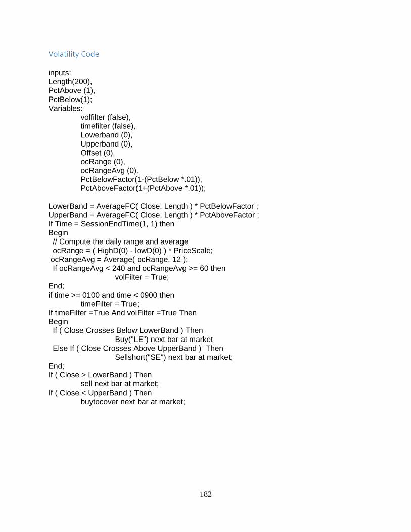
182
Volatility Code
inputs: Length(200), PctAbove (1), PctBelow(1); Variables: volfilter (false), timefilter (false), Lowerband (0), Upperband (0), Offset (0), ocRange (0), ocRangeAvg (0), PctBelowFactor(1-(PctBelow *.01)), PctAboveFactor(1+(PctAbove *.01)); LowerBand = AverageFC( Close, Length ) * PctBelowFactor ; UpperBand = AverageFC( Close, Length ) * PctAboveFactor ; If Time = SessionEndTime(1, 1) then
Begin
// Compute the daily range and average
ocRange = ( HighD(0) - lowD(0) ) * PriceScale; ocRangeAvg = Average( ocRange, 12 ); If ocRangeAvg < 240 and ocRangeAvg >= 60 then
volFilter = True; End; if time >= 0100 and time < 0900 then
timeFilter = True; If timeFilter =True And volFilter =True Then
Begin
If ( Close Crosses Below LowerBand ) Then
Buy("LE") next bar at market Else If ( Close Crosses Above UpperBand ) Then
Sellshort("SE") next bar at market; End; If ( Close > LowerBand ) Then
sell next bar at market; If ( Close < UpperBand ) Then
buytocover next bar at market;