trade policy, biotechnology and grain self-sufficiency in china

Agricultural Economics 28 (2003) 173–186

Trade policy, biotechnology and grain self-sufficiency in China

Fabrizio Fellonia, John Gilbertb, Thomas I. Wahlc,∗, Philip Wandschneiderd

a International Fund for Agricultural Development, Via del Serafico, 107, 00142 Rome, Italyb Department of Economics, Utah State University, Utah, UT, USA

c IMPACT Center, 123 Hulbert Hall, Washington State University, P.O. Box 646214, Pullman, WA 99164-6214, USAd Department of Agricultural and Resource Economics, Washington State University, Pullman, WA, USA

Received 15 January 2001; received in revised form 30 May 2002; accepted 26 June 2002

Abstract

Over the past 20 years the growth of China’s agricultural economy has been extraordinary. However, it seems unlikely thatChina will maintain self-sufficiency in grains by 2005 without substantial intervention. We develop a CGE model to assess theoptions available to Chinese policy makers. We compare the welfare effects of import tariffs and domestic support, and explorethe potential of biotechnology as a means to achieve self-sufficiency through improvements in agricultural productivity. Ourresults indicate that the price interventions that would be required to maintain China’s desired self-sufficiency ratios areconsiderable, and are unlikely to be compatible with WTO accession. The productivity improvements required are alsosignificant, and likely beyond the current potential of biotechnology.© 2002 Elsevier Science B.V. All rights reserved.

JEL classification: C68; F13; O53; Q17

Keywords: Biotechnology; Chinese agriculture; CGE

1. Introduction

Since the announcement of China’sduiwai kaifangzhengce, or ‘open door’ policy in 1978, the growth inChina’s overall and agricultural economies has beenextraordinary. Between 1979 and 1984, GDP grew byan average of 8.5% per year, accelerating to 9.7% peryear between 1985 and 1995 (a significant increaseover 1970’s levels, which averaged 4.9%). The valueof agricultural output grew by an annual average of7.5% from 1979 to 1984, and 5.6% between 1985 and1995, compared to only 2.3% between 1970 and 1978(Huang et al., 1999a). However, despite unprecedentedgrowth over the last two decades, concern has beenraised over the capacity of China to feed its population

∗ Corresponding author. Tel.:+1-509-335-6653.

in the future.Brown (1995)published the most pes-simistic predictions, evoking the spectres of soaringworld grain prices and starvation in poor countries.

While the magnitudes of Brown’s estimates havebeen seriously questioned (Fan and Agcaoili-Sombilla,1997; Yang and Huang, 1997), the emergence of asubstantial grain deficit in China is now consideredlikely. China’s grain markets are projected to ex-perience a sustained increase in demand driven bypopulation growth, rapid urbanisation, rising incomelevels and the expansion of the livestock sector as aconsequence of burgeoning meat consumption.

In the absence of intervention, the expected increasein demand for grains is unlikely to be matched bycompensating shifts in supply. There are a numberof factors which may limit supply response in China.Most important are land scarcity, the transition of land,

0169-5150/02/$ – see front matter © 2002 Elsevier Science B.V. All rights reserved.doi:10.1016/S0169-5150(02)00118-4

174 F. Felloni et al. / Agricultural Economics 28 (2003) 173–186

Nomenclature

a technological shift parameterA agricultural unskilled labourGDP/POP real GDP per capitaI investmentK capital stockL industrial unskilled labourpf factor returnr regionsS skilled labourt time period

Greek lettersδ depreciation rate on capital∆ (∆∗) aggregate labour growth rate

(target)φ convergence parameter

for (T)echnology, (L)abourλ (λ∗) factor productivity growth rate

(target)Λ marginal growth rate for

skilled/agricultural labourψ convergence parameter

(labour movement)

labour and capital to non-agricultural uses, a slow-down in yield growth, and environmental degrada-tion (erosion, salinisation). With roughly 10% of theworld’s arable land but 22% of the world’s popula-tion, China’s comparative advantage is likely to shiftfrom land-intensive commodities to labour-intensiveproducts.

Despite what economists have seen as an inevitabledecline in agricultural comparative advantage, theChinese government has set food self-sufficiency asa declared goal in its long-term plan. Although theobjective has not been clearly defined in terms of acommodity category, it has been widely interpretedas meaning that domestic production of grains shouldmeet at least 95% of domestic demand (Yang andHuang, 1997; Anderson and Peng, 1998).

Given the projections of substantial grain deficits,how can we evaluate the potential for meeting theobjective of grain self-sufficiency? Clearly, decliningself-sufficiency ratios are by no means inevitable, theyare under government control. There are (at least) three

possibilities for maintaining a given self-sufficiencylevel: border measures (tariffs), domestic support orimprovements in productivity. The first two distort theprices faced by agents in the economy, altering the in-centives to produce and/or import. Any given targetratio of grain imports can clearly be achieved, but atthe price of introducing allocative inefficiency to theeconomy. Moreover, such policies may be in conflictwith China’s accession to the World Trade Organi-sation (WTO), approved late in 2001. The researchquestion is effectively one of identifying the economiccost for China and the world economy of achievingself-sufficiency through these means.

The third possibility, productivity improvements,may arise from a variety of sources. A source of partic-ular interest is through the use of biotechnology. Theadoption of genetically modified (GM) crops offers thepotential for improved efficiency, increased yields, andreduced production costs. The key question for Chinais whether or not, given what we know about poten-tial yield increases with the adoption of GM crops andwhat we project about future grain deficits, it is feasi-ble that self-sufficiency could be attained through theuse of biotechnology.

To assess these questions we utilise a multi-regioncomputable general equilibrium (CGE) model, whichwe project to 2005 and use to simulate various policyresponses to the anticipated trade pattern. Our sim-ulation procedure accounts for accession by Chinato the Uruguay Round Agreement on Agriculture(URAA). The remainder of the paper is organised asfollows. In Section 2, we review grain supply anddemand projections for China and the implicationsof possible policy responses. InSection 3, we lookat the evidence on biotechnology as a source of pro-ductivity growth.Section 4contains a description ofthe modelling framework utilised in the paper, whileSection 5presents the results of our simulations andpolicy discussion. Finally,Section 6contains a sum-mary and concluding comments.

2. China’s grain deficit and self-sufficiencyobjectives

The agricultural reforms implemented in Chinafrom the end of the 1970s were designed to fos-ter the transition from a command economy to an

F. Felloni et al. / Agricultural Economics 28 (2003) 173–186 175

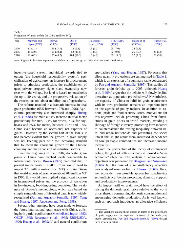
Table 1Projections of grain deficit for China (million MT)

Year Mitchell andIngco (1993)

Brown(1995)

OECF(1995)

Rosegrantet al. (1995)

ERS/USDA(1996)

Huang et al.(1999a)

Huang et al.(1999b)

2000 11 (3.1) 63 (17.7) 18 (5.1) 18 (5.1) 25 (7.0) 24 (6.8) –2005 14 (3.9) 108 (30.4) 52 (14.6) 16 (4.5) 32 (9.0) 25 (7.0) 20 (5.8)2010 22 (6.2) 155 (43.7) 104 (29.3) 15 (4.2) 39 (11.0) 27 (7.6) 20 (5.8)

Note: Figures in brackets represent the deficit as a percentage of 1995 grain domestic production.

incentive-based system: individual rewards tied tooutput (the household responsibility system), spe-cialisation of agriculture, an increase in procurementprices to stimulate production, the establishment ofquasi-private property rights (land ownership nowrests with the village, but land is leased to householdsfor up to 30 years), and the progressive relaxation ofthe restrictions on labour mobility out of agriculture.

The reforms resulted in a dramatic increase in totalgrain production (65% between 1978 and 1996). Agri-cultural productivity also increased sharply.Huanget al. (1999b)estimate a 54% increase in total factorproductivity for rice, 121% for wheat, 71% for soy-beans and 85% for maize, between 1979 and 1995.China even became an occasional net exporter ofgrains. However, by the second half of the 1980s, ithad become evident that the growth in grain supplywas not keeping pace with the increasing demandthat followed the enormous growth of the Chineseeconomy and the expansion of industrial sectors.

Since the beginning of the 1990s, domestic grainprices in China have reached levels comparable tointernational prices.Brown (1995)predicted that, ifpresent trends persist, in 2030 China would need toimport 370 million metric tons (MT) of grain. Giventhat world exports of grain were about 200 million MTin 1995, this would have implied a significant increasein international prices and the prospect of starvationin low-income, food-importing countries. The weak-ness of Brown’s methodology, which was based onsimple extrapolations of historical data, is now widelyrecognised (Fan and Agcaoili-Sombilla, 1997; Yangand Huang, 1997; Anderson and Peng, 1998).

Several other attempts have been made to forecastthe future international grain trade with China, utilis-ing both partial equilibrium (Mitchell and Ingco, 1993;OECF, 1995; Rosegrant et al., 1995; ERS/USDA,1996; Huang et al., 1999a,b) and general equilibrium

approaches (Yang and Huang, 1997). Forecasts thatallow quantity projections are summarised inTable 1,which is an extension of a summary table constructedby Fan and Agcaoili-Sombilla (1997). The studies allforecast grain deficits up to 2005, althoughHuanget al. (1999b)argue that the deficits will slowly declinethereafter, as population growth slows.1 Nevertheless,the capacity of China to fulfil its grain requirementwith its own production remains an important itemon the agenda of policy makers. In addition to na-tional pride and food security issues, motivations forthis objective include protecting China from fluctu-ations in grain prices in world markets, avoiding ashortage of foreign currency, protecting farm incomesto counterbalance the raising inequality between ru-ral and urban households and preventing the socialunrest that might result from increased dependenceon foreign staple commodities and increased incomeinequality.

From the perspective of the theory of commercialpolicy, the goal of self-sufficiency is termed a ‘non-economic’ objective. The analysis of non-economicobjectives was pioneered byBhagwati and Srinivasen(1969), but the case of a self-sufficiency objectivewas analysed even earlier byJohnson (1960). Here,we reconsider three possible approaches to achievingself-sufficiency: border protection, domestic support,and productivity improvements.

An import tariff on grain would have the effect ofraising the domestic grain price relative to the worldprice, thereby constraining domestic consumption andencouraging domestic production. As is well known,such an approach introduces an allocative efficiency

1 The variations among these studies in terms of the projectionsof grain supply can be explained in terms of the underlyingmodel assumptions.Fan and Agcaoili-Sombilla (1997)discussthese issues in detail.


(dead weight) loss to the economy, by forcing re-sources that would produce higher value elsewhereinto grain production, and by eliminating grain con-sumption where the marginal social benefit of con-sumption exceeds the marginal social cost (the worldprice) but not the marginal private cost (the domesticprice). It is therefore socially inefficient.

In effect, an import tariff is equivalent to a pro-duction subsidy combined with a consumption tax,with both applied at the same percentage rate. Eitherof these two policies could be used independently toachieve a self-sufficiency objective, although produc-tion subsidies are likely to be more palatable. A pro-duction subsidy achieves self-sufficiency exclusivelyby expanding grain production, and a consumption taxexclusively by curtailing domestic grain consumption.Clearly, either policy will introduce an allocative ef-ficiency loss. Moreover, for a given import volumetarget, and assuming substitution in production andconsumption, both a production subsidy and a con-sumption tax will be inefficient mechanisms to achieveself-sufficiency relative to a tariff because a tariff cansimultaneously exploit both methods of constrainingimports, which is the objective.

The use of both import tariffs and output subsidieson agriculture is constrained by WTO rules. Sinceit has now acceded to the WTO, China will be con-strained in its ability to raise tariffs above boundlevels. Moreover, it may face action over domesticsupport that can be shown to adversely affect tradingpartners, although there is considerably more latitudehere than in the case of tariffs. It is also likely thatpressure will continue to build in upcoming multilat-eral negotiations for agricultural trade liberalisationbeyond that committed under the URAA. Hence, inaddition to efficiency considerations, China may facepolitical constraints on the use of the price mechanismto achieve its goals.

Another way of achieving a grain self-sufficiencyobjective is to improve Chinese agricultural produc-tivity. As discussed above, the growth in China’sagricultural productivity over the period of reform hasbeen substantial, although we may debate the extentto which this merely represents moving towards theefficiency locus. Improving productivity implies noconflict with the pledge of future agricultural liberal-isation. Moreover, at least in the absence of external-ities and/or second-best effects, it should not result in

allocative efficiency losses like those associated withtariffs and domestic support.

However, productivity improvements cannot bereaped without effort, they require investment bothin research and institutional innovation, and theremay be considerable uncertainty over the end result.Furthermore, little is known about the magnitude ofproductivity improvements that would likely to berequired in order to achieve China’s self-sufficiencyobjectives. InSection 3, we consider the extent ofimprovements that have been associated with theadoption of biotechnology and genetically modifiedorganisms (GMOs).

3. Biotechnology and productivity growth

New technological processes, first developed in themid 1980s, have been adopted to develop and or mod-ify plants under commercial cultivation since 1996.Crops using biotechnology have been rapidly diffusedinto 12 countries, including six developing economies:Argentina, China, Mexico, Romania, Ukraine andSouth Africa (James, 1999). In 1999, the estimatedtotal area cultivated with GM crops was 39.9 mil-lion hectares. ‘Roundup-Ready’ (RR) soybeans weregrown on 21.6 million hectares of land (54% of worldGM-planted area),Bacillus Thuringiensis (Bt) cornon 11.1 (28%), Bt cotton on 3.7 (9%), and RR canolaon 3.4 (9%).2 GM crops are concentrated in threecountries (USA, Argentina, Canada), accounting foralmost 99% of the total GM-planted area.

China’s GM crop production was still extremelysmall in 1999, with only 0.1% of the domestic croparea cultivated with GM varieties, and a share ofonly 1% of the GM-planted area in the 12 coun-tries. However, between 1998 and 1999, the growthin the area cultivated with transgenic varieties inChina was 300%, evidence of the growing interest in

2 Bt corn and cotton have been genetically modified to producethe toxins of theBacillus Thuringiensis (Bt), a bacterium frequentlypresent in the soils. Such toxins have strong inhibitory effectson digestion in parasites as the European corn borer and noundesirable effects on mammals. However, the diffusion of Bt cornhas been associated with a higher mortality of monarch butterfly, anon-targeted insect (Losey et al., 1999). The DNA of RR soybeanand canola has been modified in order to develop resistance toglyphosate, a non-selective herbicide.


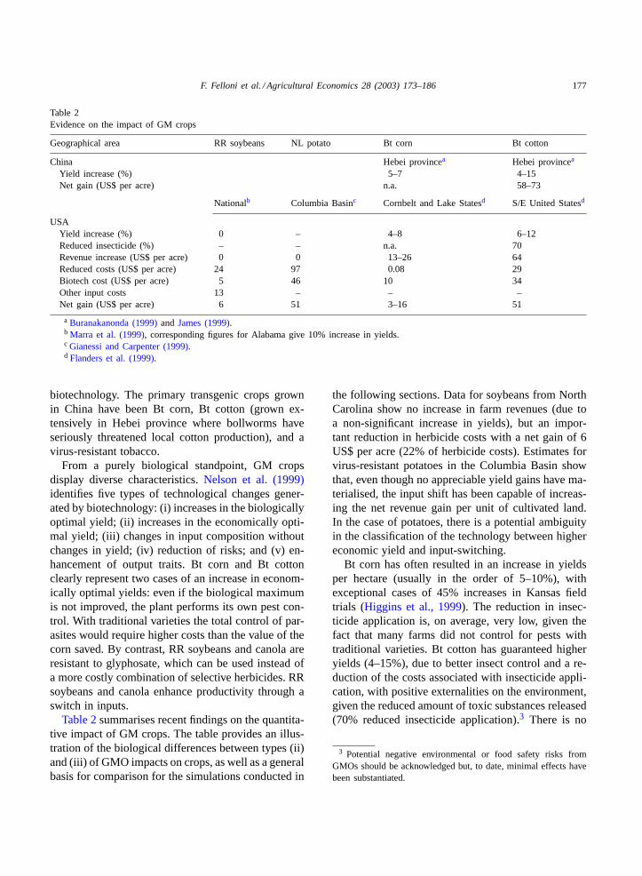
Table 2Evidence on the impact of GM crops

Geographical area RR soybeans NL potato Bt corn Bt cotton

China Hebei provincea Hebei provincea

Yield increase (%) 5–7 4–15Net gain (US$ per acre) n.a. 58–73

Nationalb Columbia Basinc Cornbelt and Lake Statesd S/E United Statesd

USAYield increase (%) 0 – 4–8 6–12Reduced insecticide (%) – – n.a. 70Revenue increase (US$ per acre) 0 0 13–26 64Reduced costs (US$ per acre) 24 97 0.08 29Biotech cost (US$ per acre) 5 46 10 34Other input costs 13 – – –Net gain (US$ per acre) 6 51 3–16 51

a Buranakanonda (1999)and James (1999).b Marra et al. (1999), corresponding figures for Alabama give 10% increase in yields.c Gianessi and Carpenter (1999).d Flanders et al. (1999).

biotechnology. The primary transgenic crops grownin China have been Bt corn, Bt cotton (grown ex-tensively in Hebei province where bollworms haveseriously threatened local cotton production), and avirus-resistant tobacco.

From a purely biological standpoint, GM cropsdisplay diverse characteristics.Nelson et al. (1999)identifies five types of technological changes gener-ated by biotechnology: (i) increases in the biologicallyoptimal yield; (ii) increases in the economically opti-mal yield; (iii) changes in input composition withoutchanges in yield; (iv) reduction of risks; and (v) en-hancement of output traits. Bt corn and Bt cottonclearly represent two cases of an increase in econom-ically optimal yields: even if the biological maximumis not improved, the plant performs its own pest con-trol. With traditional varieties the total control of par-asites would require higher costs than the value of thecorn saved. By contrast, RR soybeans and canola areresistant to glyphosate, which can be used instead ofa more costly combination of selective herbicides. RRsoybeans and canola enhance productivity through aswitch in inputs.

Table 2summarises recent findings on the quantita-tive impact of GM crops. The table provides an illus-tration of the biological differences between types (ii)and (iii) of GMO impacts on crops, as well as a generalbasis for comparison for the simulations conducted in

the following sections. Data for soybeans from NorthCarolina show no increase in farm revenues (due toa non-significant increase in yields), but an impor-tant reduction in herbicide costs with a net gain of 6US$ per acre (22% of herbicide costs). Estimates forvirus-resistant potatoes in the Columbia Basin showthat, even though no appreciable yield gains have ma-terialised, the input shift has been capable of increas-ing the net revenue gain per unit of cultivated land.In the case of potatoes, there is a potential ambiguityin the classification of the technology between highereconomic yield and input-switching.

Bt corn has often resulted in an increase in yieldsper hectare (usually in the order of 5–10%), withexceptional cases of 45% increases in Kansas fieldtrials (Higgins et al., 1999). The reduction in insec-ticide application is, on average, very low, given thefact that many farms did not control for pests withtraditional varieties. Bt cotton has guaranteed higheryields (4–15%), due to better insect control and a re-duction of the costs associated with insecticide appli-cation, with positive externalities on the environment,given the reduced amount of toxic substances released(70% reduced insecticide application).3 There is no

3 Potential negative environmental or food safety risks fromGMOs should be acknowledged but, to date, minimal effects havebeen substantiated.


guarantee that in future trials similar outcomes willoccur, and it is important to remember that the valuespresented inTable 2are contingent upon the specificgeo-climatic conditions of the concerned geographi-cal areas and the endemic plant diseases and pests.Nevertheless, the results provide us with perspectiveon the potential effect of adoption of GM crops.

4. Overview of the modelling approach

Although our principal interest in this paper is thegrain sectors, we have highlighted the role of growthof non-agricultural sectors in drawing resources outof agriculture, reflecting the anticipated decline inChina’s comparative advantage in land-intensivecrops. We have also noted the role of increasing con-sumption of meat products as a driver of increasedgrain demand. Moreover, trade policy changes underthe URAA, which China will implement as part ofits WTO accession agreement, go beyond the grainsector in terms of both direct coverage and indirectfeedback effects. This suggests that general equilib-rium techniques are an appropriate analytical tool foranalysing policy responses to projected grain deficits.

Computable general equilibrium or CGE modelsare numerical implementations of general equilibriumtheory. By integrating real world data with a com-plete structural description of the behaviour of agentswithin an economic system and the constraints thatthey face, CGE models allow quantitative examina-tion of the effect of policy interventions within a con-sistent framework that accounts for important marketinterrelationships and second-best interactions. CGEmodels have been widely used in analysing China’strade policy reforms (Gilbert and Wahl, 2002).

The model that we utilise in this paper was intro-duced inGilbert et al. (2000), and falls into a categorythat is termedrecursive dynamic CGE. This meansthat the model solves iteratively, finding an equilib-rium solution in each period, and then updating thegrowth parameters before searching for the next equi-librium. Agents in this class of model do not optimisein an intertemporal context. In this section, we focuson the simulation assumptions and data, and discussthe structural features of the model only briefly. Amore comprehensive description of the model struc-ture is contained inAppendix A.

The intra-period (equilibrium) model has been de-veloped from the work ofRutherford (1998). It is aperfectly competitive model, based on relatively stan-dard assumptions. The model is multi-regional, andin each region there is a single agent for governmentspending, investment, and household consumption.Each sector within each region is represented by a sin-gle competitive firm producing with constant returnsto scale technology and making zero profits. Constantelasticity of substitution (CES) functions representproduction, while a Stone–Geary utility function rep-resents household demand (allowing us to specifynon-unitary income elasticities). International tradeis modelled along Armington lines, meaning that do-mestic production and imports (as well as importsfrom alternative sources) are treated as imperfect sub-stitutes (CES functions are used to produce the com-posites). The model is closed by allowing factor pricesto adjust to maintain full employment of endowments,by exogenising government expenditures and currentaccount balances, and by letting regional savings be aconstant fraction of income. The recursive dynamicsupdate the values of endowments (capital and laboursupply) and technical change parameters in responseto the results of the previous solution, and/or a presetpath. Further details can be found inAppendix A.

The initial equilibrium data used in the model isfrom the GTAP4 database (McDougall et al., 1998).We aggregate the database to 15 sectors (paddyrice, wheat, other grains, vegetables and fruit, othernon-grain crops, livestock, forestry, fisheries, pro-cessed rice, meat products, dairy products, otherfood products, light manufactures, heavy manufac-tures and services), 15 regions (Australia, Canada,China, Europe, Indonesia, Japan, Malaysia, Mexico,New Zealand, other APEC, Philippines, Republic ofKorea, Thailand, United States and ROW), and fiveendowment commodities (skilled labour, unskilledlabour, land, natural resources and capital) with agri-cultural and industrial unskilled labour distinguished.Substitution parameters are also from GTAP4, withthe exception that the Armington elasticities at bothlevels have been doubled to provide a better projec-tion over the long-run (as inAnderson et al., 1997).We supplement the data with information on agri-cultural and non-agricultural labour counts from theFAOSTAT database, using the skill breakdowns inLiu et al. (1998) to obtain consistent measures of


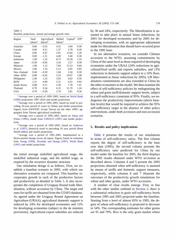
Table 3Baseline projections, annual percentage growth rates

Region Totallaboura

Agriculturallabourb

Skilledlabourc

Capitald TFPe

Australia 0.80 −0.55 4.55 3.94 0.30Canada 0.60 0.21 1.37 3.78 0.30China 0.83 0.47 2.61 13.04 1.26Europe 0.00 −1.31 4.49 3.40 0.30Indonesia 1.69 1.33 8.75 10.29 1.33Japan −0.30 −0.85 3.54 3.27 0.30Malaysia 1.90 1.12 7.83 12.53 0.60Mexico 2.06 1.16 5.13 4.05 0.83New Zealand 0.40 −0.20 1.84 3.34 0.30Other APEC 0.80 −0.42 5.22 10.07 1.08Philippines 2.40 1.22 5.93 4.62 0.50ROW 1.51 0.99 5.21 6.55 0.92South Korea 0.88 0.11 5.39 7.78 1.01Thailand 0.79 0.34 6.31 11.70 1.24USA 0.70 −0.28 2.79 2.81 0.30

a Average over a period of 1995–2005, based onWorld Bank(1999) projections 1997–2010 and model projections.

b Average over a period of 1995–2005, based on trend in pre-ceding 10-year period (5 years in China) and model projections.Figures from FAOSTAT, except Taiwan (in the other APEC ag-gregate) from Taiwan agricultural yearbooks.

c Average over a period of 1995–2005, based onAhuja andFilmer (1995), trends fromUNESCO (1997)and model projec-tions.

d Average over a period of 1995–2005, based onAndersonet al. (1997), historical trend in preceding 10 year period (PennWorld tables) and model projections.

e Average over a period of 1995–2005. Implemented as aHicks-neutral change across all inputs. Figures based on estimatesfrom Young (1994), Drysdale and Huang (1997), World Bank(1997) and model projections.

the initial average unskilled agricultural wage, theunskilled industrial wage, and the skilled wage, asrequired by the recursive dynamic structure.

Our simulation design is as follows. First, we es-tablish a baseline scenario to 2005, with which ouralternative scenarios are compared. This baseline in-corporates growth in each of the productive factorsand productivity as detailed inTable 3. It also incor-porates the completion of Uruguay Round trade liber-alisation, without accession by China. The target endrates for tariffs are obtained from the GTAP3 database.As agreed under the Uruguay Round Agreement onAgriculture (URAA), agricultural domestic support isreduced by 24% for developed economies and 13%for developing economies (subject to the de minimisprovisions). Agricultural export subsidies are reduced

by 36 and 24%, respectively. The liberalisation is as-sumed to take place in annual linear reductions, by2001 for developed economies and by 2005 for de-veloping economies, with an appropriate adjustmentmade for liberalisation that should have occurred priorto the 1995 base.

In our alternative scenarios, we consider Chineseaccession to the WTO, assuming commitments byChina of the same level as those required of developingeconomies under the URAA (24% reductions in agri-cultural/food tariffs and exports subsidies, and 13%reductions in domestic support subject to a 10% floor,implemented as linear reductions by 2005). UR liber-alisation commitments are also extended to China bythe other economies in the model. We then examine theeffect of self-sufficiency policies by endogenising thewheat and grain tariff/domestic support levels, subjectto a self-sufficiency constraint of 95%. Finally, we en-dogenise the productivity improvements (above base-line levels) that would be required to achieve the 95%self-sufficiency target in the absence of other policyinterventions, under both accession and non-accessionscenarios.

5. Results and policy implications

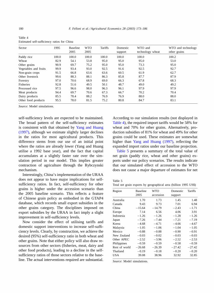
Table 4 presents the results of our simulationsin terms of self-sufficiency ratios. The first columnreports the degree of self-sufficiency in the baseyear data (1995), the second column presents theself-sufficiency ratio predicted for China by ourmodel under the baseline for 2005, the third displaysthe 2005 results obtained under WTO accession asdescribed above. Columns 4 and 5 present the 2005projections obtained when self-sufficiency is attainedby means of tariffs and domestic support measures,respectively, while columns 6 and 7 illustrate theoutcomes of the productivity growth simulations forwheat and other grains, under WTO accession.

A number of clear results emerge. First, in linewith the other studies outlined inSection 2, there isa substantial reduction in grain self-sufficiency levelsbetween 1995 and 2005 projected under the baseline.Starting from a level of almost 83% in 1995, the de-gree of wheat self-sufficiency is projected to decreaseto 54%. The corresponding estimates for other grainsare 91 and 70%. Rice is the only grain market where


Table 4Estimated self-sufficiency ratios for China

Sector 1995 Baseline2005

WTO2005

Tariffs Domesticsupport

WTO andtechnology wheat

WTO and technologyother grains

Paddy rice 100.0 100.0 100.0 100.0 100.0 100.0 100.2Wheat 82.9 54.1 53.8 95.0 95.0 95.0 53.0Other grains 90.9 69.7 75.2 95.0 95.0 73.3 95.0Vegetables and fruits 99.9 93.4 93.0 92.5 91.6 92.5 92.7Non-grain crops 91.5 66.8 63.6 63.6 60.5 61.9 62.7Other livestock 99.6 88.3 88.1 86.3 85.8 87.7 87.9Forestry 97.0 70.6 68.9 69.0 66.3 67.8 68.3Fisheries 92.8 51.6 49.5 50.1 48.7 49.0 49.2Processed rice 97.5 96.6 98.0 96.3 96.1 97.9 97.9Meat products 94.4 69.7 70.6 67.3 66.7 70.2 70.4Dairy products 85.5 78.4 88.2 76.9 76.9 88.0 88.0Other food products 95.5 78.0 81.5 75.2 80.8 84.7 83.1

Source: Model simulations.

self-sufficiency levels are expected to be maintained.The broad pattern of the self-sufficiency estimatesis consistent with that obtained byYang and Huang(1997), although we estimate slightly larger declinesin the ratios for most agricultural products. Thisdifference stems from our use of an initial pointwhere the ratios are already lower (Yang and Huangutilise a 1992 base year), and the fact that capitalaccumulates at a slightly faster rate over the sim-ulation period in our model. This implies greatercontraction of agriculture through the Rybczynskimechanism.

Interestingly, China’s implementation of the URAAdoes not appear to have major implications for self-sufficiency ratios. In fact, self-sufficiency for othergrains is higher under the accession scenario thanthe 2005 baseline scenario. This reflects a featureof Chinese grain policy as embodied in the GTAP4database, which records small export subsidies in theother grains category. The disciplines imposed onexport subsidies by the URAA in fact imply a slightimprovement in self-sufficiency levels.

Now consider the effect of utilising tariffs anddomestic support interventions to increase self-suffi-ciency levels. Clearly, by construction, we achieve thedesired (95%) self-sufficiency ratio in both wheat andother grains. Note that either policy will also draw re-sources from other sectors (fisheries, meat, dairy andother food products), leading to a decline in the self-sufficiency ratios of those sectors relative to the base-line. The actual interventions required are substantial.

According to our simulation results (not displayed inTable 4), the required import tariffs would be 58% forwheat and 70% for other grains. Alternatively, pro-duction subsidies of 81% for wheat and 49% for othergrains could be used. These estimates are somewhathigher thanYang and Huang (1997), reflecting theexpanded import ratios under our baseline projection.

Table 5presents a summary of the total value ofnet grain (paddy rice, wheat and other grains) ex-ports under our policy scenarios. The results indicatethat our simulated effect of accession to the WTOdoes not cause a major departure of estimates for net

Table 5Total net grain exports by geographical area (billion 1995 US$)

Region Baseline2005

WTOaccession

Domesticsupport

Tariffs

Australia 1.70 1.73 1.45 1.48Canada 9.43 9.73 7.01 6.94China −15.64 −14.79 −2.43 −1.71Europe 7.14 6.56 4.06 3.91Indonesia −1.26 −1.26 −1.28 −1.26Japan −7.26 −7.44 −7.21 −7.19Korea −4.68 −4.71 −4.66 −4.67Malaysia −1.05 −1.06 −1.04 −1.05Mexico −0.88 −0.88 −0.90 −0.91New Zealand −0.03 −0.02 −0.03 −0.03Other APEC −2.52 −3.96 −2.52 −2.53Philippines −0.59 −0.59 −0.58 −0.59Rest of world −26.68 −26.39 −27.42 −27.42Thailand −0.19 −0.18 −0.20 −0.20USA 39.08 38.96 32.92 32.85



grain exports from the corresponding values for the2005 baseline (in fact, the value of net imports fallsslightly). Columns 3 and 4 show that the impositionof higher tariffs or the adoption of domestic supportwould dramatically reduce the value of net imports ofgrain, from 15.6 (under the 2005 baseline assumption)to 2.4 and 1.7 billion US$ (bUS$) under the tariff anddomestic support policies, respectively. Out of the15 regions that we consider in our model, Canada,Europe and the United States appear to be the mostaffected by a self-sufficiency policy. In particular, USnet exports of grain are estimated to decrease from39 bUS$ under the baseline to 32.9 and 32.8 bUS$,respectively.

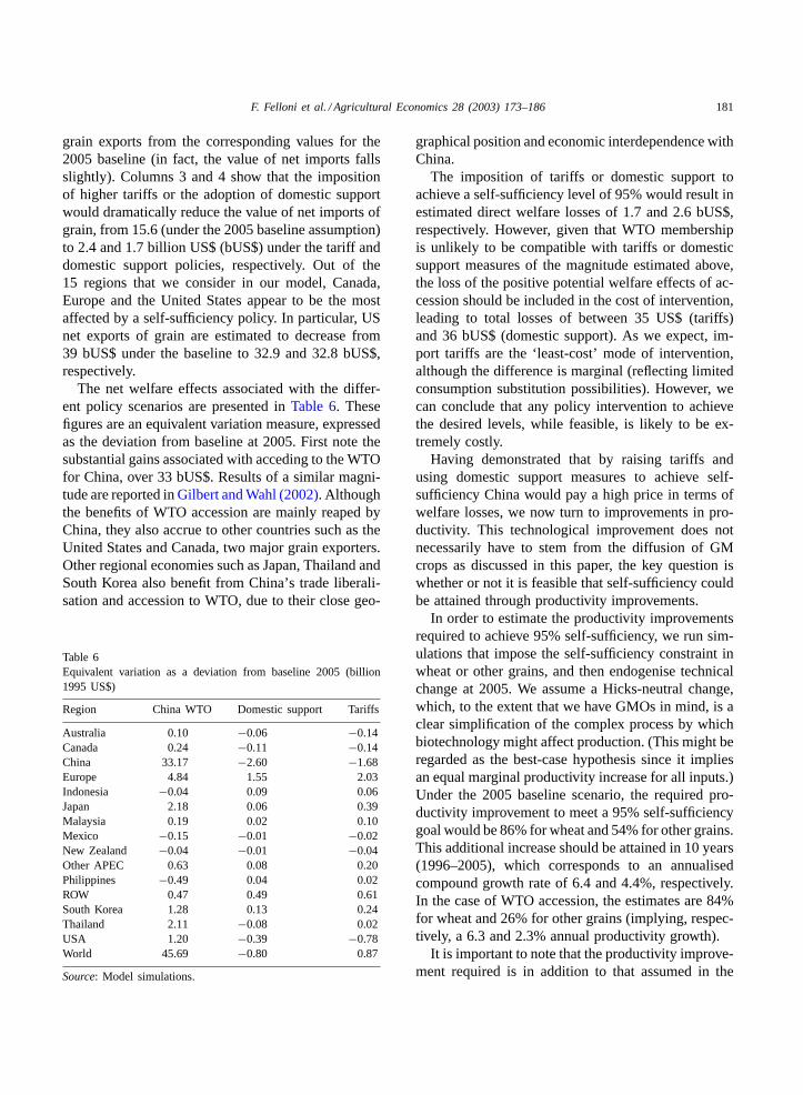
The net welfare effects associated with the differ-ent policy scenarios are presented inTable 6. Thesefigures are an equivalent variation measure, expressedas the deviation from baseline at 2005. First note thesubstantial gains associated with acceding to the WTOfor China, over 33 bUS$. Results of a similar magni-tude are reported inGilbert and Wahl (2002). Althoughthe benefits of WTO accession are mainly reaped byChina, they also accrue to other countries such as theUnited States and Canada, two major grain exporters.Other regional economies such as Japan, Thailand andSouth Korea also benefit from China’s trade liberali-sation and accession to WTO, due to their close geo-

Table 6Equivalent variation as a deviation from baseline 2005 (billion1995 US$)

Region China WTO Domestic support Tariffs

Australia 0.10 −0.06 −0.14Canada 0.24 −0.11 −0.14China 33.17 −2.60 −1.68Europe 4.84 1.55 2.03Indonesia −0.04 0.09 0.06Japan 2.18 0.06 0.39Malaysia 0.19 0.02 0.10Mexico −0.15 −0.01 −0.02New Zealand −0.04 −0.01 −0.04Other APEC 0.63 0.08 0.20Philippines −0.49 0.04 0.02ROW 0.47 0.49 0.61South Korea 1.28 0.13 0.24Thailand 2.11 −0.08 0.02USA 1.20 −0.39 −0.78World 45.69 −0.80 0.87


graphical position and economic interdependence withChina.

The imposition of tariffs or domestic support toachieve a self-sufficiency level of 95% would result inestimated direct welfare losses of 1.7 and 2.6 bUS$,respectively. However, given that WTO membershipis unlikely to be compatible with tariffs or domesticsupport measures of the magnitude estimated above,the loss of the positive potential welfare effects of ac-cession should be included in the cost of intervention,leading to total losses of between 35 US$ (tariffs)and 36 bUS$ (domestic support). As we expect, im-port tariffs are the ‘least-cost’ mode of intervention,although the difference is marginal (reflecting limitedconsumption substitution possibilities). However, wecan conclude that any policy intervention to achievethe desired levels, while feasible, is likely to be ex-tremely costly.

Having demonstrated that by raising tariffs andusing domestic support measures to achieve self-sufficiency China would pay a high price in terms ofwelfare losses, we now turn to improvements in pro-ductivity. This technological improvement does notnecessarily have to stem from the diffusion of GMcrops as discussed in this paper, the key question iswhether or not it is feasible that self-sufficiency couldbe attained through productivity improvements.

In order to estimate the productivity improvementsrequired to achieve 95% self-sufficiency, we run sim-ulations that impose the self-sufficiency constraint inwheat or other grains, and then endogenise technicalchange at 2005. We assume a Hicks-neutral change,which, to the extent that we have GMOs in mind, is aclear simplification of the complex process by whichbiotechnology might affect production. (This might beregarded as the best-case hypothesis since it impliesan equal marginal productivity increase for all inputs.)Under the 2005 baseline scenario, the required pro-ductivity improvement to meet a 95% self-sufficiencygoal would be 86% for wheat and 54% for other grains.This additional increase should be attained in 10 years(1996–2005), which corresponds to an annualisedcompound growth rate of 6.4 and 4.4%, respectively.In the case of WTO accession, the estimates are 84%for wheat and 26% for other grains (implying, respec-tively, a 6.3 and 2.3% annual productivity growth).

It is important to note that the productivity improve-ment required is in addition to that assumed in the


baseline (our assumed productivity growth in grainproduction in China averages 1.3% over the simulationperiod). Obviously, these are substantial requirements.By comparison, between 1979 and 1995, productiv-ity for wheat, maize and soybeans grew at an annualrate of 5.1, 3.9 and 3.4%, respectively (Huang et al.,1999b). However, the rapid improvements in produc-tivity that accompanied the move to market-orientationover this period are unlikely to be duplicated.

What about the potential of biotechnology? The re-quired productivity shifts computed in our simulationsfar exceed the results provided by field trials and sur-vey results from GM technology. We do not possessclear data on the productivity gains on new geneticallymodified varieties of wheat, because they are currentlyunder experimentation and private firms are reluctantto release such information. Nonetheless, possible op-timal biological yield improvements in the region of10–30% have been claimed (Hoisington et al., 1999;Jackson, 1999). Even if such values were confirmed,the gain in productivity required for self-sufficiencyin wheat would still be almost three times higher (andlikely to continue to grow as China’s industrial econ-omy expands).

Regarding other grains, aggregation in our modelimplies a category comprising diverse cereals, forsome of which no genetically modified varieties havebeen tested. At a first glance, the required productivitygain of 26% under the accession scenario may seemmore realistic, given the fact that yield gains higherthan 15% have been observed for Bt corn. Neverthe-less we must be cautious: very high yields have beenreported only under experimental conditions, whileincreases in the order of 5–10% are normally observ-able in actual commercial cultivation. It also has tobe assumed that in China a 10–20% ‘refuge practice’will be adopted; a proportion (refuge) of the fields willhave to be planted with non-Bt corn in order to retardthe development of parasite resistance toBacillusThuringiensis toxins that would thwart the adoptionof the technology. It is also important to consider thatyield increases for commercial application are oftencalculated as averages of cross-sectional data and itis often impossible to control for different input com-binations and other relevant variables such as the soiltypes. Our results therefore suggest that the requiredtechnological shift in other grains is also unlikely tobe attainable through GM adoption alone, by 2005.

As an alternative, the Chinese government mightconsider the less ambitious goal of preserving the 1995level of self-sufficiency for wheat (82.9%) and othergrains (90.9%), respectively. According to our simu-lations, under the baseline scenario, the required ad-ditional productivity growth would be 44% for wheatand 41% (3.7 and 3.5% annually) for other grains,while, for the WTO accession case, the correspondingvalues are 44% for wheat and 19% (3.7 and 1.8% an-nually) for other grains. With respect to other grains,the required technological shifts, although still high,are closer to observed values.

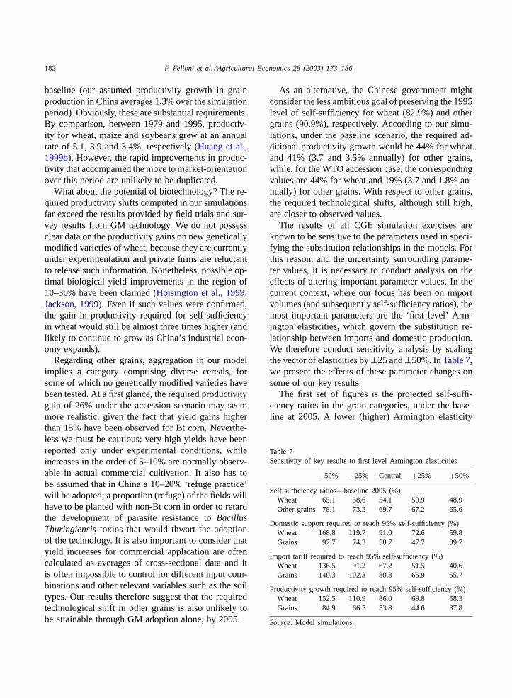
The results of all CGE simulation exercises areknown to be sensitive to the parameters used in speci-fying the substitution relationships in the models. Forthis reason, and the uncertainty surrounding parame-ter values, it is necessary to conduct analysis on theeffects of altering important parameter values. In thecurrent context, where our focus has been on importvolumes (and subsequently self-sufficiency ratios), themost important parameters are the ‘first level’ Arm-ington elasticities, which govern the substitution re-lationship between imports and domestic production.We therefore conduct sensitivity analysis by scalingthe vector of elasticities by±25 and±50%. InTable 7,we present the effects of these parameter changes onsome of our key results.

The first set of figures is the projected self-suffi-ciency ratios in the grain categories, under the base-line at 2005. A lower (higher) Armington elasticity

Table 7Sensitivity of key results to first level Armington elasticities

−50% −25% Central +25% +50%

Self-sufficiency ratios—baseline 2005 (%)Wheat 65.1 58.6 54.1 50.9 48.9Other grains 78.1 73.2 69.7 67.2 65.6

Domestic support required to reach 95% self-sufficiency (%)Wheat 168.8 119.7 91.0 72.6 59.8Grains 97.7 74.3 58.7 47.7 39.7

Import tariff required to reach 95% self-sufficiency (%)Wheat 136.5 91.2 67.2 51.5 40.6Grains 140.3 102.3 80.3 65.9 55.7

Productivity growth required to reach 95% self-sufficiency (%)Wheat 152.5 110.9 86.0 69.8 58.3Grains 84.9 66.5 53.8 44.6 37.8



implies that domestic production and imports areless (more) substitutable, this implies higher (lower)self-sufficiency ratios under the baseline projection.However, even with the elasticities halved, the declineremains significant, at 65% for wheat and 78% forother grains (compared with 83 and 91% in the baseyear).

While lower Armington elasticities result in smallerreductions in the estimated self-sufficiency ratios,they also increase the estimated difficulty of attain-ing the 95% objective. In the case of a tariff, thelower (higher) the elasticity, the higher (lower) theprice change required to induce a given quantityshift in imports. The pattern is similar for the otherpolicies.

In assessing the robustness of our results, we notethat even with the Armington elasticities increased by50% (triple the original levels in GTAP4), the domes-tic support or tariffs required for 95% self-sufficiencyrange between 40 and 60%, which is well beyond whatis likely to be acceptable under China’s WTO acces-sion agreement. Similarly, the productivity improve-ments required (at 58 and 38%) remain well outsidethe potential of GMOs, and will be difficult to attain.We are therefore confident that, while our numericalresults may vary somewhat over the range of feasibleparameter values, our general policy conclusions arequite robust.

6. Concluding comments

To assess the feasibility of China’s grain self-sufficiency objectives, we have analysed bor-der measures, domestic support and productivityimprovements using a CGE simulation model. In in-terpreting the results of CGE simulations, the usualcaveats need to be borne in mind. Given the uncer-tainty over specification, we should concentrate ourattention on the broad patterns that emerge and themagnitudes of the estimates, which in this case arerobust to parameter changes.

As in the existing literature, our projections indi-cate that it is unlikely that China under the currentregime will be able to produce enough grains to sat-isfy national demand by 2005. If China wishes toattain 95% self-sufficiency, it will need to put in placemechanisms to increase production and/or decrease

consumption. The two obvious policy candidates(tariffs and domestic support) will inflict heavy eco-nomic costs on China and may be at odds with WTOmembership. By contrast, productivity increaseswould enhance China’s economic gains and be com-patible with the WTO, the only question is one ofattainability.

We have contrasted our simulation findings withthe empirical values observed for GMO technologyin field trials and commercial cultivation. The datahave been obtained from several survey areas, mak-ing it is difficult to control for differences in inputcomposition. We therefore treat the values as ref-erence benchmarks. Nevertheless, serious questionshave been raised. Our simulations indicate that inorder to meet a 95% self-sufficiency requirement,productivity increases would have to be substantiallyhigher than these reference benchmarks. When we as-sume the less ambitious objective of maintaining the1995 self-sufficiency level for wheat and other grains,the projected values become closer to those claimedor observed in field trials. Of course, productivitygrowth cannot be reduced to the diffusion of GMcrops and we cannot not exclude the possibility thatother technological improvements may lead to self-sufficiency.

While our findings suggest that adoption ofGM crops is unlikely to be sufficient to attainself-sufficiency, GM technology does present inter-esting opportunities for Chinese agriculture. Growersmay benefit from higher yields, enhanced productquality, reduced exposure to climatic hazards, and aless expensive input mix. Since GMOs can reduce theapplication of herbicides and insecticides, their im-pact on the environment should also not be ignored.Likewise, there are also risks associated with GMOs.While largely speculative at this time, both the actualenvironmental and safety risks and consumer percep-tions must be closely monitored. These are complexissues that warrant further study.

7. Disclaimer

The opinions expressed in this paper are solely thoseof the authors and do not necessarily reflect the opin-ions or orientations of the institutions to which theybelong.


Acknowledgements

We would like to thank the anonymous referees forvery helpful comments. Any remaining errors are ourown.

Appendix A

In this appendix, we describe the recursive dynamicCGE model that was used to generate the results in thispaper. The intra-period model is based onRutherford(1998), and is of a well-established class. We there-fore describe it in greatly streamlined form, followingGilbert and Wahl (2002). The global economy con-sists ofM regions indexed byr. Let V r be a vector(lengthF) of factor endowments in each regionr, andP r be a vector (lengthN) of prices in each region.We can define the GNP functions for each region asGr(P r,V r ) = max{P r · Y r : V r}, and the expendi-ture functions asEr(P r , Ur) = min{P r · Dr : Ur},whereUr is aggregate utility in regionr. The budgetconstraints are then:

Sr(P r ,V r , Ur) = G(P r ,V r ) − Er(P r , Ur) = 0

r = 1, . . . ,M (A.1)

where we have fixed the current account balance atzero. From the first order conditions to the GNP max-imisation problem, we obtain sectoral supply functionsby Hotelling’s lemma, and Hicksian demand functionsfollow similarly from the expenditure function, hence:

Sri (P

r ,V r , Ur) = Dri (P

r , Ur) − Y ri (P

r ,V r )

i = 1, . . . , N; r = 1, . . . ,M (A.2)

define Hicksian net exports. With trade there can beonly one price vector (P ). Equilibrium requires:

M∑r=1

Sri (P ,V r , Ur) = 0 i = 1, . . . , N. (A.3)

By Walras’ law these equilibrium conditions are notindependent, and any one of them can be dropped.Hence, one element ofP (sayP1) must be declared anuméraire price. The solution to the system of equa-tions defined by (A.1)–(A.3) then yields a relativeprice vector, aggregate utility levels, and net exports.

We can subsequently derive factor prices from theGNP function:

Wrj = Wr

j (P ,V r )

j = 1, . . . , F ; r = 1, . . . ,M. (A.4)

In this simple model, we haveM+MN+N+2MF−1variables, but we have onlyM + MN + N + MF − 1independent equations. In a neoclassical closure, theV r are declared exogenous, enabling the system to besolved.

The simulation model adds considerable complex-ity, but does not alter this basic framework. Pro-duction utilises intermediate inputs. Final demandsare distinguished between households, government,trade, and capital creation. There is imperfect sub-stitution between foreign and domestic goods, andbetween alternative sources of imports (the Arming-ton assumption)—and thus a three-stage optimisationprocedure in both intermediate and final demand. Spe-cific functional forms define the substitution relation-ships (CES functions in value-added and Armington,Leontief in intermediate use, Stone–Geary in house-hold demand). Finally, distortions are introduced tothe system by allowing taxes and subsidies to drivewedges between the prices faced by the various agentsin the system.

The Eqs. (A.5)–(A.13)that make up the recursivedynamics of the model are given below:

λtr = λ∗ + (λ0

r − λ∗)φTr

(GDPt−1r /POPt−1

r )φTr

(A.5)

∆tr = ∆∗ + (∆0

r − ∆∗)φLr

(GDPt−1r /POPt−1

r )φLr

(A.6)

ΛtSr = Λ0

Sr

{1 − (pf t−1Lr /pf t−1

Sr )}ψSL

{1 − (pf 0Lr/pf 0

Sr)}ψSL(A.7)

ΛtAr = Λ0

Ar{1 − (pf t−1

Lr /pf t−1Ar )}ψAL

{1 − (pf 0Lr/pf 0

Ar)}ψAL(A.8)

atr = eλ

tr t (A.9)

Str = St−1

r (1 + ∆tr)(1 + Λt

Sr) (A.10)

Atr = At−1

r (1 + ∆tr)(1 + Λt

Ar) (A.11)


Ltr = (1 + ∆t

r)Lt−1r +

(pf 0

Lr

pf 0Ar

)At−1

r ΛtAr

−(

pf 0Lr

pf 0Sr

)St−1r Λt

Sr (A.12)

Ktr = (1 − δr )K

t−1r + I t−1

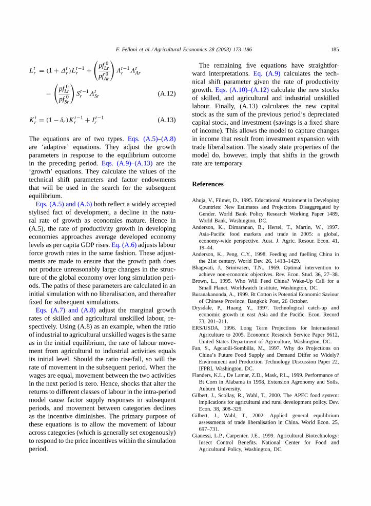
r (A.13)

The equations are of two types.Eqs. (A.5)–(A.8)are ‘adaptive’ equations. They adjust the growthparameters in response to the equilibrium outcomein the preceding period.Eqs. (A.9)–(A.13)are the‘growth’ equations. They calculate the values of thetechnical shift parameters and factor endowmentsthat will be used in the search for the subsequentequilibrium.

Eqs. (A.5) and (A.6)both reflect a widely acceptedstylised fact of development, a decline in the natu-ral rate of growth as economies mature. Hence in(A.5), the rate of productivity growth in developingeconomies approaches average developed economylevels as per capita GDP rises.Eq. (A.6)adjusts labourforce growth rates in the same fashion. These adjust-ments are made to ensure that the growth path doesnot produce unreasonably large changes in the struc-ture of the global economy over long simulation peri-ods. The paths of these parameters are calculated in aninitial simulation with no liberalisation, and thereafterfixed for subsequent simulations.

Eqs. (A.7) and (A.8)adjust the marginal growthrates of skilled and agricultural unskilled labour, re-spectively. Using (A.8) as an example, when the ratioof industrial to agricultural unskilled wages is the sameas in the initial equilibrium, the rate of labour move-ment from agricultural to industrial activities equalsits initial level. Should the ratio rise/fall, so will therate of movement in the subsequent period. When thewages are equal, movement between the two activitiesin the next period is zero. Hence, shocks that alter thereturns to different classes of labour in the intra-periodmodel cause factor supply responses in subsequentperiods, and movement between categories declinesas the incentive diminishes. The primary purpose ofthese equations is to allow the movement of labouracross categories (which is generally set exogenously)to respond to the price incentives within the simulationperiod.

The remaining five equations have straightfor-ward interpretations.Eq. (A.9) calculates the tech-nical shift parameter given the rate of productivitygrowth. Eqs. (A.10)–(A.12)calculate the new stocksof skilled, and agricultural and industrial unskilledlabour. Finally, (A.13) calculates the new capitalstock as the sum of the previous period’s depreciatedcapital stock, and investment (savings is a fixed shareof income). This allows the model to capture changesin income that result from investment expansion withtrade liberalisation. The steady state properties of themodel do, however, imply that shifts in the growthrate are temporary.

References

Ahuja, V., Filmer, D., 1995. Educational Attainment in DevelopingCountries: New Estimates and Projections Disaggregated byGender. World Bank Policy Research Working Paper 1489,World Bank, Washington, DC.

Anderson, K., Dimaranan, B., Hertel, T., Martin, W., 1997.Asia-Pacific food markets and trade in 2005: a global,economy-wide perspective. Aust. J. Agric. Resour. Econ. 41,19–44.

Anderson, K., Peng, C.Y., 1998. Feeding and fuelling China inthe 21st century. World Dev. 26, 1413–1429.

Bhagwati, J., Srinivasen, T.N., 1969. Optimal intervention toachieve non-economic objectives. Rev. Econ. Stud. 36, 27–38.

Brown, L., 1995. Who Will Feed China? Wake-Up Call for aSmall Planet. Worldwatch Institute, Washington, DC.

Buranakanonda, A., 1999. Bt Cotton is Potential Economic Saviourof Chinese Province. Bangkok Post, 26 October.

Drysdale, P., Huang, Y., 1997. Technological catch-up andeconomic growth in east Asia and the Pacific. Econ. Record73, 201–211.

ERS/USDA, 1996. Long Term Projections for InternationalAgriculture to 2005. Economic Research Service Paper 9612,United States Department of Agriculture, Washington, DC.

Fan, S., Agcaoili-Sombilla, M., 1997. Why do Projections onChina’s Future Food Supply and Demand Differ so Widely?Environment and Production Technology Discussion Paper 22,IFPRI, Washington, DC.

Flanders, K.L., De Lamar, Z.D., Mask, P.L., 1999. Performance ofBt Corn in Alabama in 1998, Extension Agronomy and Soils.Auburn University.

Gilbert, J., Scollay, R., Wahl, T., 2000. The APEC food system:implications for agricultural and rural development policy. Dev.Econ. 38, 308–329.

Gilbert, J., Wahl, T., 2002. Applied general equilibriumassessments of trade liberalisation in China. World Econ. 25,697–731.

Gianessi, L.P., Carpenter, J.E., 1999. Agricultural Biotechnology:Insect Control Benefits. National Center for Food andAgricultural Policy, Washington, DC.


Higgins, R., Buschman, L., Sloderbeck, P., Hayden, S., Martin,V., 1999. Evaluation of Corn Borer Resistance and Grain Yieldfor the Bt and Non-Bt Hybrids. Department of Entomology,Kansas State University.

Hoisington, D., Khairallah, M., Reeves, T., Ribaut, J.M.,Skovmand, B., 1999. Plant Genetic Resources: What can TheyContribute Toward Increased Crop Productivity? InternationalMaize and Wheat Improvement Center, Mexico City.

Huang, J., Rozelle, S., Rosegrant, M.W., 1999a. China’s foodeconomy to the twenty-first century: supply, demand, and trade.Econ. Dev. Cultural Change 47, 737–766.

Huang, J., Rozelle, S., Tuan, F., 1999b. China’s agriculture, tradeand productivity in the 21st century. In: Wahl, T., Fuller,F. (Eds.), Chinese Agriculture and the WTO. Proceedings ofWCC-101 Meeting. Seattle, Washington, December 1999.

Jackson, J., 1999. Crop-Boosting Discovery is as Low as PondScum. The Orlando Sentinel, 29 January.

James, C., 1999. Global Review of Commercialized TransgenicCrops. ISAAA, Ithaca, 1999.

Johnson, H.G., 1960. The cost of protection and the scientifictariff. J. Political Econ. 68, 327–345.

Liu, J., Van Leeuwen, N., Vo, T.T., Tyers, R., Hertel, T., 1998.Disaggregating labour payments by skill level. In: McDougall,R., Elbehri, A., Truong, T.P. (Eds.), Global Trade, Assistance,and Protection: The GTAP4 Data Base. Center for Global TradeAnalysis, Purdue University.

Losey, J.E., Rayor, L.S., Carter, M.E., 1999. Transgenic pollenharms monarch larvae. Nature 399, 214.

Marra, M., Carlson, G., Hubbel, B., 1999. Economic Impacts ofthe First Crop Biotechnologies. Department of Agricultural andResource Economics, North Carolina State University.

McDougall, R.A., Elbehri, A., Truong, T.P. (Eds.), 1998. GlobalTrade, Assistance, and Protection: The GTAP4 Data Base.Center for Global Trade Analysis, Purdue University.

Mitchell, D., Ingco, M., 1993. World Food Outlook. InternationalEconomics Department, World Bank, Washington, DC.

Nelson, G.C., De Pinto, A., Bullock, D., Nitsi, E.I., Rosegrant, M.,Josling, T., Babinard, J., Cunningham, C., Unnevehr, L., Hill,L., 1999. The Economics and Politics of Genetically ModifiedOrganisms in Agriculture: Implications for WTO 2000. Officeof Research Bulletin 809, University of Illinois College ofAgricultural, Consumer and Environmental Sciences.

OECF, 1995. Prospects for Grain Supply–Demand Balanceand Agricultural Development Policy. Overseas EconomicCooperation Fund, Research Institute of DevelopmentAssistance, Tokyo, Japan.

Rosegrant, M., Agacaoili-Sombilla, M., Perez, N., 1995. GlobalFood Projections to 2020: Implications for Investment. 2020Vision Discussion Paper 5, International Food Policy ResearchInstitute, Washington, DC.

Rutherford, T., 1998. GTAP in GAMS: The Dataset and StaticModel. Department of Economics, University of Colorado.

UNESCO, 1997. Statistical Yearbook. United Nations Educational,Scientific and Cultural Organisation, Paris.

World Bank, 1997. Global Economic Prospects and the DevelopingCountries. World Bank, Washington, DC.

World Bank, 1999. World Development Indicators. World Bank,Washington, DC.

Yang, Y., Huang, Y., 1997. How should China feed itself? WorldEcon. 20, 913–934.

Young, A., 1994. Lessons from the east Asian NICs: a contrarianview. Eur. Econ. Rev. 38, 964–973.

trade policy, biotechnology and grain self-sufficiency in china

Documents