i

Trade Liberalization, Poverty and Welfare in Pakistan

Inaugural Dissertation submitted

as the requirement

for the degree of

PhD International Development Studies (IDS)

at the

Institute of Development Research

and Development Policy

Ruhr-University Bochum

Submitted by

Naveed Ahmed Shaikh

Bochum 2011

ii

Table of Contents

List of Figures v

List of Tables vi

Abbreviations viii

Words of Thanks ix

1 Introduction 1

2 International Trade-Labour Income Inequality, Prices, and Poverty 8

2.1 Trade-Growth-Income Distribution-Poverty Nexus 8

2.2 Trade-Price-Wage-Poverty Nexus 11

2.3 Stolper-Samuelson (S-S) Theory and Heckscher-Ohlin (H-O) Model 13

2.3.1 Assumptions and Implications of the Chosen Approach 14 2.3.2 Implications of the Model 19

2.4 Evidence from the Literature 20 2.4.1 Evidence from Latin America 21 2.4.2 Evidence from Asia 23

2.5 Discussion on Empirical Evidence 25

3 Choice of Methodological Technique 27

3.1 Computable General Equilibrium (CGE) Analysis 28

3.2 Partial Equilibrium Analysis 33

3.3 Micro Macro (Simulation) Models 36

3.4 Choice of an appropriate Modeling Technique 38

4 Trade Liberalization, Prices of Traded and Nontraded Goods, Households’ Labour Income, Welfare, and Poverty 41

4.1 Interrelations between International Trade, Domestic Prices, and Factor Prices 42

4.1.1 Domestic Prices of Traded Goods 42

iii

4.1.2 Domestic Prices of Nontraded Goods 44 4.1.3 Households’ Labour Income 45

4.2 Trade Liberalization, Household Demand, and Welfare Effects 58

4.2.1 Household Expenditure 58 4.2.2 Change in Marshallian Consumers’ Surplus 63 4.2.3 Change in Hicksian Compensating Variation 65 4.2.4 Change in the Households’ Labour Income 67 4.2.5 Change in Poorest Households’ Welfare 69

5 Statistical Results and Interpretation 72

5.1 Data 73 5.1.1 Import Tariff and International and Domestic Prices 73 5.1.3 Domestic Prices and Labour Income 78 5.1.4 Exclusion of Goods from the Model 79

5.2 Regression Analysis 80

5.3 Change in the Domestic Prices of Traded and Nontraded Goods and Households’ Demand 82

5.3.1 Change in the Domestic Prices of Traded Goods 82 5.3.2 Change in the Domestic Prices of Nontraded Goods 84 5.3.3 Household Demand Equations and the Change in Demand

for the Selected Traded and Nontraded goods 87 5.3.3.1 Estimated Marshallian Demand 89 5.3.3.2 Estimated Hicksian Demand 93

5.4 Trade Liberalization, Household Welfare, Poorest Household Welfare and Labour incomes 96

5.4.1 Welfare Measuring Approaches 96 5.4.2 Marshallian Consumer Surplus (MCS) 99 5.4.3 Hicksian Compensating Variation (HCV) 102 5.4.4 Poorest Households’ Demand and Welfare (MCS) 107 5.5 Labour Incomes and the Domestic Prices of the Selected

Goods 111 5.6 Total (Price and Labour income) Effect on Household

Welfare 119

5.7 Discussion on the Statistical Results 124

5.8 Limitations of the Study 129

6 Summary and Policy Recommendations 131

iv

Bibliography 136

Appendix 146

A1 Data and Other Descriptive Tables 146

A2 Estimated Demand Equations 154

A3 Detailed tables on empirical estimations of demands and domestic prices including tariff 156

A4 Detailed Tables on Import Tariff and Calculation of Commodity-wise Tariff Following the Tariff in the General Economy 165

A5 Detailed tables on welfare loss due to selective protectionist trade policy in selected traded goods 172

A6 Domestic Prices, Production and Trade of selected goods for 1970-2005 176

v

List of Figures

Fig. 1: Customs revenue in percent of imports (C.I.F) in Pakistan (1992-2005) 2

Fig. 2: PCI-Trend in Pakistan (1992-2005) 2

Fig. 3: Commodity-groups wise actual tariff in PKR per ton calculated by dividing the collected tariff revenue in PKR by the import quantities in tons (3-11) 4

Fig. 4: Relative commodity prices determine the wage-rent ratio 17

Fig. 5: Factor-Price diagram with unit cost curves (left) with no Factor Intensity Reversals and (right) with Factor Intensity Reversals 49

Fig. 6: Factor-Price Diagram reflecting change in factor price (wage) due to change in one good's price while holding the prices of other goods constant. [Suranovic (2010)] 54

Fig. 7: A Linear case of 2x2x2 in Factor-Price Diagram 56

Fig. 8: Locating the lowest level of household expenditure to attain a utility level "u" 59

Fig. 9: The Hicksian and Marshallian demands for good X1 when its price P1 is falling 61

Fig. 10: Estimated and calculated domestic prices at average and real tariff rates for the available years 76

Fig. 11: Average percentage sector-wise employment in Pakistan from 1970-2005 (Various Labour Force Surveys) 117

Fig. 12: Average sector-wise employment of unskilled workers in Pakistan 1970-2005 (Various Labour Force Surveys) 118

vi

List of Tables

Table 1: 14-Year average domestic prices calculated at average actual and falling general import tariff rates (PKR per Ton) given average international prices and percent difference in both tariffs 83

Table 2: Empirical link between domestic price of electricity and the domestic prices of traded goods 85

Table 3: Empirical link between domestic price of firewood and the domestic prices of traded goods 85

Table 4: Average estimated domestic prices of nontraded goods at actual and at general falling tariff 87

Table 5: Percentage shares of monthly household expenditure for commodities from various sectors 88

Table 6: Estimated linear and natural log linear Marshallian demand equations 91

Table 7: Average Estimated Marshallian demand quantities in tons at actual tariff and at the falling general tariff 92

Table 8: Average Estimated Hicksian demand quantities in tons at actual tariff and at the falling general tariff 94

Table 9: Total and per household change in MCS due to the selective protectionist trade policy in the selected commodities 1992-2005 100

Table 10: Yearly total and average change in welfare under MCS to the ordinary Pakistani household 101

Table 11: Total and per household change in HCV due to the selective protectionist trade policy in the selected commodities 1992-2005 103

Table 12: Yearly total change in HCV and change in HCV per average Pakistani household 104

Table 13: Comparison of Total HCV and MCS in PKR 105

vii

Table 14: 14 year total sum of the poorest household demand quantities (KGs) of the selected goods at actual tariff and when the tariff follows the general falling tariff 108

Table 15: Single poorest household’s change in MCS due to the selective protectionist trade policy 1992-2005 109

Table 16: Year-wise change in MCS of a single poorest household in all selected traded and nontraded goods due to protectionist trade policy 110

Table 17: Empirical link between labour incomes in agriculture and the domestic prices 112

Table 18: Empirical link between labour incomes in manufacturing and estimated domestic prices 113

Table 19: Estimated agriculture labour income with domestic prices at actual tariff and at domestic prices if the general falling tariff is applied 113

Table 20: Estimated manufacturing labour income with domestic prices at actual tariff and at domestic prices if the general falling tariff is applied 115

Table 21: Inter-sector labour income correlation 118

Table 22: Net change in an ordinary household’s labour income due to the protection 120

Table 23: Total yearly loss to an ordinary Pakistani household due to the selective protectionist policy 121

Table 24: Total welfare loss to the poorest Pakistani household due to the protectionist policy 122

viii

Abbreviations

CGE Computable General Equilibrium

C.I.F Cost Insurance and Freight

CUM Cubic Meter

D-W Durbin Watson

FAO Food and Agriculture organization

FBS Federal Bureau of Statistics

FGT Foster Greer Thorbecke indicators

Fig. Figure

GDP Gross Domestic Product

GTAP Global Trade Analysis project

H-O Heckscher-Ohlin

HCV Hicksian Compensating Variations

HEC Higher Education Commission

IDS International Development Studies

ILO International Labour Organization

MCS Marshallian Consumer Surplus

OLS Ordinary Least Squares

PCI Per Capita Income

PKR Pakistani Rupee

SAM Social Accounting Matrix

S-S Stolper-Samuelson

ix

Words of Thanks

I am pleased to acknowledge the kind assistance, scholarly guidance, and

help of many people and institutions by expressing my heartfelt gratitude

and thankfulness toward them.

The first amongst the individuals, who supported, helped, and inspired me

throughout my doctoral thesis is my PhD supervisor, Prof. Dr. Wilhelm

Löwenstein. Indeed it was his continuous support and active supervision at

every stage of this piece of writing that enabled me to accomplish such

advanced research work. I am even more indebted to him especially for

his kind consideration for sparing extra and spontaneous spans of time

during the final weeks before submission of the thesis. Secondly, I pay

special thanks to Prof. Em. Dr. Dieter Bender for being co-supervisor of

my thesis. Thirdly, I would take the opportunity to acknowledge the

enlightening discussion(s) with Dr. Tobias Bidlingmeier, one of my

colleagues at Institute of Development Research and Development Policy,

Ruhr-University Bochum, working on a similar topic, on issues related to

model building and variable identification at early stages of my work.

In Pakistan my sincere thanks go to Dr. Ghulam Murtaza Khuhro, Deputy

Commissioner, Income Tax, Karachi for his support in collecting

statistical books, annual reports, and other published materials from the

library of Statistical Division of Pakistan, Karachi Branch. My special

thanks go to Mr. Bashir Ahmed Zia, Chief Librarian who took special

efforts and invested time in getting the bundles of data Chapters from

various annual surveys and reports photocopied and sending me in

Germany at State Bank’s expenses on my request.

Amongst institutions, I express my earnest thankfulness to Higher

Education Commission of Pakistan for its financial assistance for five

x

years that facilitated me to earn my PhD in Germany. Secondly, my thanks

proceed for DAAD (German Academic Exchange Service) for smoothing

my placement as a PhD student at the Institute of Development Research

and Development Policy, Ruhr-University Bochum and my stay in

Germany throughout the study period. I admit that without DAAD

support, stay in Germany would not have been as pleasant and

comfortable as it was.

The present PhD International Development Studies (IDS) program

included a three-month field survey for data collection in Pakistan. Being

a member of the Ruhr University Research School1 at Ruhr University

Bochum, my field survey trip to Pakistan was funded from the annual

allowance of the Ruhr University Research School. Further, different

workshops and seminars offered by Ruhr Research School played a great

role in creating a serious research environment amongst PhD scholars

from the variety of disciplines. The workshop I found most useful while

writing my PhD thesis was on becoming a better academic writer. For all

this I extend my heartfelt gratitude for Dr. Ursula Justus, Counseling (PhD

Planning and Funding Opportunities) and Ms. Maria Sprung, Assistant

from Ruhr Research School, for their support.

I also thank the staff of State Bank of Pakistan, Central Directorate,

Central Library administration for absolute cooperation in accessing the

books, journals, and annual reports during my visit there.

Last but not least, I express my thanks for the staff and colleagues at

Institute of Development Research and Development Policy for extending

a cooperative and helping hand whenever I approached them.

At the end, I would like to mention the support and the help extended from

my loving wife, Shamshad Naveed. Despite that she was student of Master

1 http://www.research-school.rub.de/about_us.html

xi

of Science in Computer Engineering at Duisburg-Essen University,

Duisburg Campus, she took care of me, our home and our child during my

busy schedules. I also want to mention the prayers and motivation of my

father back in Pakistan which have always encouraged me and have been a

source of resilience in my life.

Naveed Ahmed Shaikh,

IEE, Bochum, 2011

1

1 Introduction

Recent decades have observed rapid expansion in the monetary worth of

the world economy. With the inception of the era of economic

globalization since the last two decades of the 20th century, countries have

drawn closer to each other for more trade integration and economic

cohesion. Though the swollen volume of global trade may have brought

fortunes for the world economy and for some individual countries2

(Example: export-oriented growth in East Asian countries after

liberalizing trade during the 1960s and 1970s) nevertheless it has raised

several matters of serious concern regarding the impact of globally freer

trade on the poverty situation, with special emphasis on developing

countries. Some of the crucial questions confronting researchers in the

fields of development studies and international trade are: Does enhanced

volume of global trade help control the global poverty rate? Or do open

developing countries outperform the closed ones in attaining the national

poverty targets and pursuing the well being for their populations? Do poor

masses in developing countries benefit from the international trade and

lose from protectionist policies? To reach some reasonable conclusions

regarding trade-poverty and wage inequality links (Sections 2.1 and 2.2) in

light of the above mentioned questions, an intensive literature survey is

conducted and presented in section 2.4. Existing literature on the

experience of several developing countries with liberalizing trade regimes

provides an inconclusive blend of arguments with findings for and against

the liberal policies. The case of Latin American and Asian countries’

liberal trade policies is discussed in sections 2.4.1 and 2.4.2.

2 Ahmed, J. (2001) has found a strong two way causality between exports and income growth. The discussion on issues related with trade-growth causality is provided in section 2.1.

%

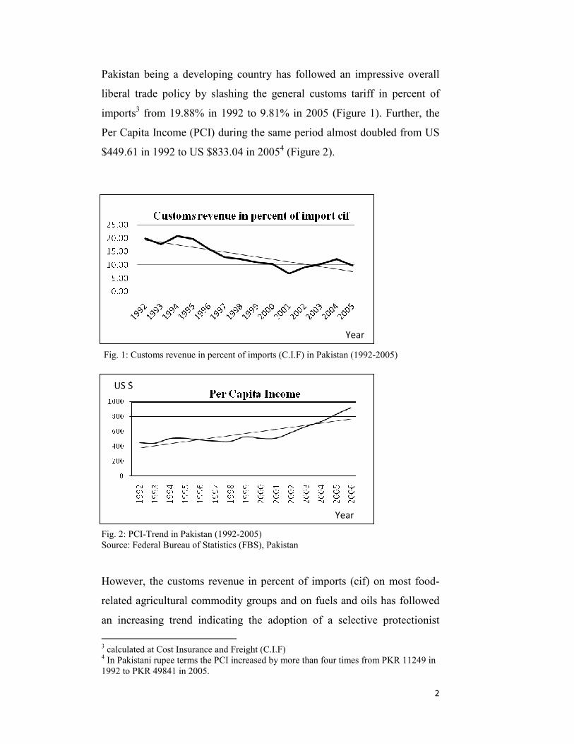
Pakistan being a developing country has followed an impressive overall

liberal trade policy by slashing the general customs tariff in percent of

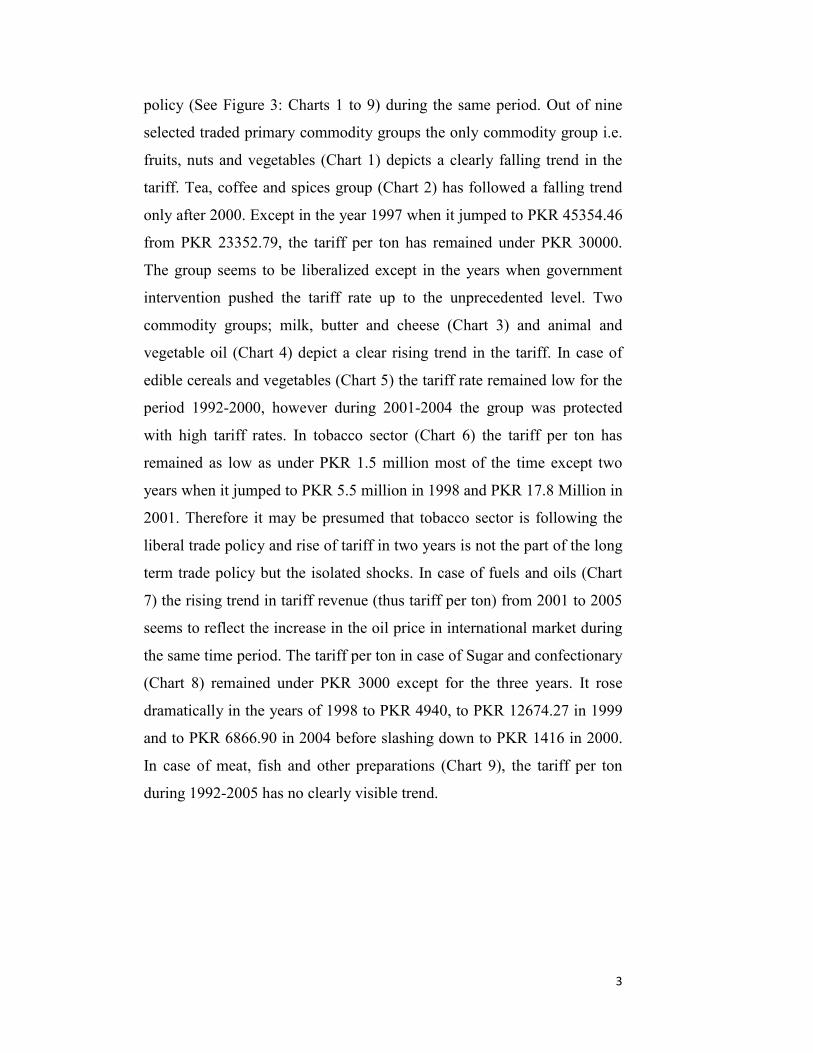
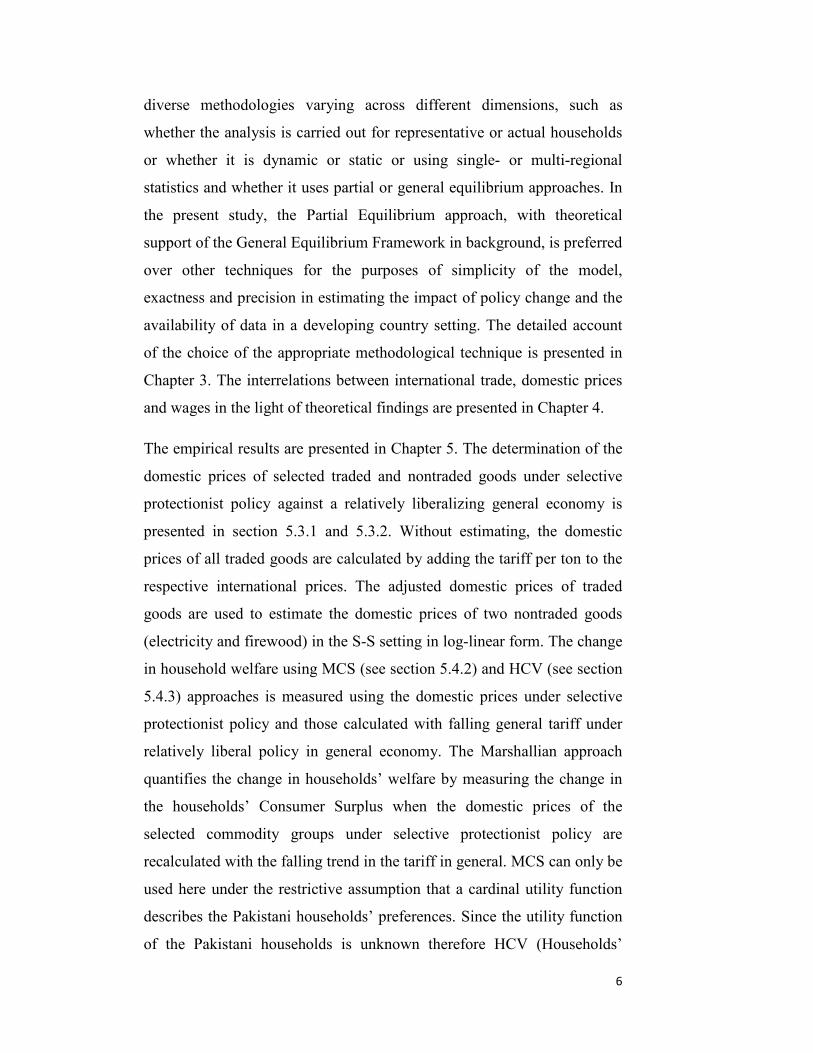
imports3 from 19.88% in 1992 to 9.81% in 2005 (Figure 1). Further, the

Per Capita Income (PCI) during the same period almost doubled from US

$449.61 in 1992 to US $833.04 in 20054 (Figure 2).

Fig. 1: Customs revenue in percent of imports (C.I.F) in Pakist

Fig. 2: PCI-Trend in Pakistan (1992-2005) Source: Federal Bureau of Statistics (FBS), Pakistan

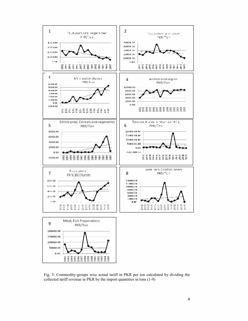
However, the customs revenue in percent of impor

related agricultural commodity groups and on fuels

an increasing trend indicating the adoption of a

3 calculated at Cost Insurance and Freight (C.I.F) 4 In Pakistani rupee terms the PCI increased by more than four 1992 to PKR 49841 in 2005.

Year Year

an (1992-2005)

Year

US $

t

s

t

2

s (cif) on most food-

and oils has followed

elective protectionist

imes from PKR 11249 in

3

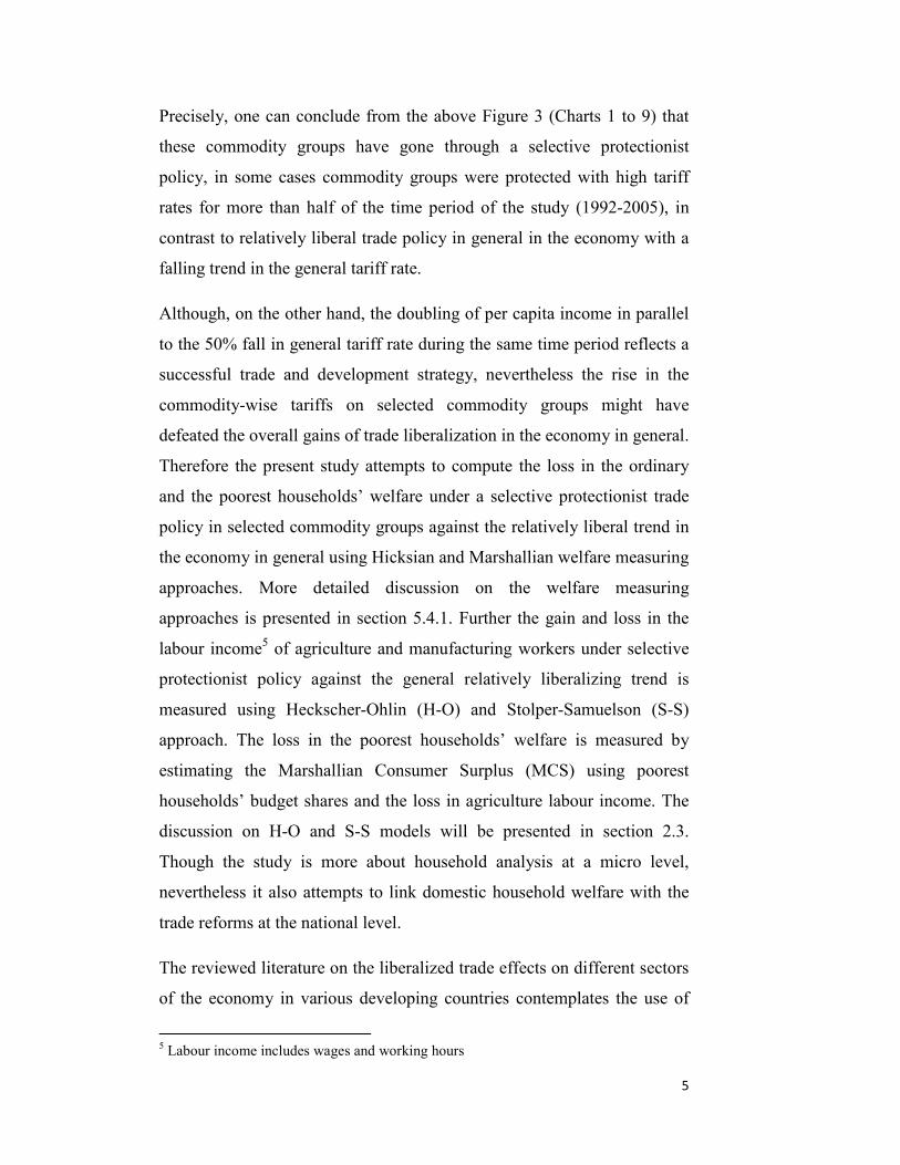
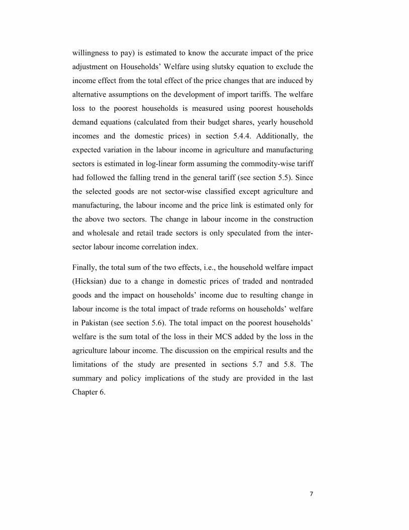
policy (See Figure 3: Charts 1 to 9) during the same period. Out of nine

selected traded primary commodity groups the only commodity group i.e.

fruits, nuts and vegetables (Chart 1) depicts a clearly falling trend in the

tariff. Tea, coffee and spices group (Chart 2) has followed a falling trend

only after 2000. Except in the year 1997 when it jumped to PKR 45354.46

from PKR 23352.79, the tariff per ton has remained under PKR 30000.

The group seems to be liberalized except in the years when government

intervention pushed the tariff rate up to the unprecedented level. Two

commodity groups; milk, butter and cheese (Chart 3) and animal and

vegetable oil (Chart 4) depict a clear rising trend in the tariff. In case of

edible cereals and vegetables (Chart 5) the tariff rate remained low for the

period 1992-2000, however during 2001-2004 the group was protected

with high tariff rates. In tobacco sector (Chart 6) the tariff per ton has

remained as low as under PKR 1.5 million most of the time except two

years when it jumped to PKR 5.5 million in 1998 and PKR 17.8 Million in

2001. Therefore it may be presumed that tobacco sector is following the

liberal trade policy and rise of tariff in two years is not the part of the long

term trade policy but the isolated shocks. In case of fuels and oils (Chart

7) the rising trend in tariff revenue (thus tariff per ton) from 2001 to 2005

seems to reflect the increase in the oil price in international market during

the same time period. The tariff per ton in case of Sugar and confectionary

(Chart 8) remained under PKR 3000 except for the three years. It rose

dramatically in the years of 1998 to PKR 4940, to PKR 12674.27 in 1999

and to PKR 6866.90 in 2004 before slashing down to PKR 1416 in 2000.

In case of meat, fish and other preparations (Chart 9), the tariff per ton

during 1992-2005 has no clearly visible trend.

Fc

9

ig. 3: Commodity-groups wise actual tariff in ollected tariff revenue in PKR by the import qua

8

7

6

5

4

3

2

1

4

PKR per ton calculated by dividing the ntities in tons (1-9)

5

Precisely, one can conclude from the above Figure 3 (Charts 1 to 9) that

these commodity groups have gone through a selective protectionist

policy, in some cases commodity groups were protected with high tariff

rates for more than half of the time period of the study (1992-2005), in

contrast to relatively liberal trade policy in general in the economy with a

falling trend in the general tariff rate.

Although, on the other hand, the doubling of per capita income in parallel

to the 50% fall in general tariff rate during the same time period reflects a

successful trade and development strategy, nevertheless the rise in the

commodity-wise tariffs on selected commodity groups might have

defeated the overall gains of trade liberalization in the economy in general.

Therefore the present study attempts to compute the loss in the ordinary

and the poorest households’ welfare under a selective protectionist trade

policy in selected commodity groups against the relatively liberal trend in

the economy in general using Hicksian and Marshallian welfare measuring

approaches. More detailed discussion on the welfare measuring

approaches is presented in section 5.4.1. Further the gain and loss in the

labour income5 of agriculture and manufacturing workers under selective

protectionist policy against the general relatively liberalizing trend is

measured using Heckscher-Ohlin (H-O) and Stolper-Samuelson (S-S)

approach. The loss in the poorest households’ welfare is measured by

estimating the Marshallian Consumer Surplus (MCS) using poorest

households’ budget shares and the loss in agriculture labour income. The

discussion on H-O and S-S models will be presented in section 2.3.

Though the study is more about household analysis at a micro level,

nevertheless it also attempts to link domestic household welfare with the

trade reforms at the national level.

The reviewed literature on the liberalized trade effects on different sectors

of the economy in various developing countries contemplates the use of

5 Labour income includes wages and working hours

6

diverse methodologies varying across different dimensions, such as

whether the analysis is carried out for representative or actual households

or whether it is dynamic or static or using single- or multi-regional

statistics and whether it uses partial or general equilibrium approaches. In

the present study, the Partial Equilibrium approach, with theoretical

support of the General Equilibrium Framework in background, is preferred

over other techniques for the purposes of simplicity of the model,

exactness and precision in estimating the impact of policy change and the

availability of data in a developing country setting. The detailed account

of the choice of the appropriate methodological technique is presented in

Chapter 3. The interrelations between international trade, domestic prices

and wages in the light of theoretical findings are presented in Chapter 4.

The empirical results are presented in Chapter 5. The determination of the

domestic prices of selected traded and nontraded goods under selective

protectionist policy against a relatively liberalizing general economy is

presented in section 5.3.1 and 5.3.2. Without estimating, the domestic

prices of all traded goods are calculated by adding the tariff per ton to the

respective international prices. The adjusted domestic prices of traded

goods are used to estimate the domestic prices of two nontraded goods

(electricity and firewood) in the S-S setting in log-linear form. The change

in household welfare using MCS (see section 5.4.2) and HCV (see section

5.4.3) approaches is measured using the domestic prices under selective

protectionist policy and those calculated with falling general tariff under

relatively liberal policy in general economy. The Marshallian approach

quantifies the change in households’ welfare by measuring the change in

the households’ Consumer Surplus when the domestic prices of the

selected commodity groups under selective protectionist policy are

recalculated with the falling trend in the tariff in general. MCS can only be

used here under the restrictive assumption that a cardinal utility function

describes the Pakistani households’ preferences. Since the utility function

of the Pakistani households is unknown therefore HCV (Households’

7

willingness to pay) is estimated to know the accurate impact of the price

adjustment on Households’ Welfare using slutsky equation to exclude the

income effect from the total effect of the price changes that are induced by

alternative assumptions on the development of import tariffs. The welfare

loss to the poorest households is measured using poorest households

demand equations (calculated from their budget shares, yearly household

incomes and the domestic prices) in section 5.4.4. Additionally, the

expected variation in the labour income in agriculture and manufacturing

sectors is estimated in log-linear form assuming the commodity-wise tariff

had followed the falling trend in the general tariff (see section 5.5). Since

the selected goods are not sector-wise classified except agriculture and

manufacturing, the labour income and the price link is estimated only for

the above two sectors. The change in labour income in the construction

and wholesale and retail trade sectors is only speculated from the inter-

sector labour income correlation index.

Finally, the total sum of the two effects, i.e., the household welfare impact

(Hicksian) due to a change in domestic prices of traded and nontraded

goods and the impact on households’ income due to resulting change in

labour income is the total impact of trade reforms on households’ welfare

in Pakistan (see section 5.6). The total impact on the poorest households’

welfare is the sum total of the loss in their MCS added by the loss in the

agriculture labour income. The discussion on the empirical results and the

limitations of the study are presented in sections 5.7 and 5.8. The

summary and policy implications of the study are provided in the last

Chapter 6.

8

2 International Trade-Labour Income Inequality, Prices, and Poverty

The body of literature analyzed during the study is broadly classified into

two segments: one segment deals with the impact of trade on the country’s

national economic growth. From this channel, however, the poor can only

gain proportionately from enhanced growth, given that there are no

income distributional transformations after trade reforms. The second

segment offers analysis of the trade-poverty link via changes in domestic

prices of traded and nontraded goods and wages. Since trade liberalization

affects household welfare by altering domestic prices of traded and

nontraded goods and wages of workers in various sectors of the economy,

the present study bases trade patterns of Pakistan with rest of the world on

the H-O model, and the link of trade with domestic prices and labour

incomes is determined from the S-S theorem. The present Chapter is

divided into two parts. The first part describes the theoretical approach of

the S-S theory and the H-O model. The second part discusses existing

evidence on the impact of liberalized trade policy on wages, prices, and

economic growth. Prior to making any proceedings with the subject

matter, it seems logical to first look at the transmission channels through

which trade affects poverty. For a detailed discussion on the links between

global trade and poverty see Harrison, A. and McMillan, M. (2007).

2.1 Trade-Growth-Income Distribution-Poverty Nexus

The (indirect channel) link between trade, growth and poverty is quite well

established in the literature. Several studies [such as Dollar and Kraay

(2001) and Sachs et. al. (1995)] claim that trade is good for the economic

growth of developing countries and that open economies outperform

9

closed ones in achieving rapid economic growth. Esfahani (1991) has

concluded that export expansion resulting from trade reforms leads to the

availability of more imports, which spurs output in semi-industrialized

countries. The argument put forward to verify the former claim is based on

comparison between performance of Latin America and East Asia during

1965-19896 on three key variables- namely GDP growth rate, annual rate

of growth in the manufacturing sector, and growth in national exports.

Latin American countries followed the dictates of import substitution

policy and showed poor performance in contrast to rapidly growing East

Asian countries implementing an outward oriented strategy. In addition,

some studies found a predominantly positive relationship between exports

and economic growth by employing cross country regression analysis.7

On the other hand, there is evidence that global economic growth along

with the spread of technological innovation and the substantial diminution

of the barriers to international trade are regarded as the raison d’être of the

rise in the volume of global trade to historically unprecedented levels.

Rodriguez, F. and Rodrik, D. (1999), Ravallion (2004), Agenore (2002)

and others tend to contest the generalized mainstream view about the

causal association between trade and growth. They recommend

methodological improvements in empirical strategies and supplementary

social protection policies to ripen the fruits of trade. The problems with

using export volumes in these regressions are the endogeneity of trade and

the undetermined exports-economic growth causality, since trade is not

exogenous but rather is influenced by various other factors, especially

economic growth.

The issue of endogeneity and causality of trade and growth is tackled in

Frankel and Romer (1999) by introducing the geographical factor as the

instrument variable for trade. It assumes that geographical distance

6 World Bank (1989, 1990). Also cited in Edwards (1993). 7 See Edwards (1993) for review of the related literature.

10

influences trade volume but is independent of income (growth). Their

results demonstrate a positive but statistically weak link between trade and

income and therefore cannot be delivered as a rigorous proof8.

Rodriguez, F. and Rodrik, D. (1999) further took a skeptical approach

toward the causal association between trade reforms and economic growth

and showed that geography can influence other important factors such as

institutions besides trade. Therefore it cannot be concluded that trade

causes rise in income. However, they found a slightly negative

relationship between import duty and economic growth rate using data

from 124 countries from 1975-1994. Even though studies applying

geographical distances to predict trade shares obtain rigorous results, still

one cannot definitively say that trade causes a rise in income.

Ravallion (2004), by using cross country comparisons and aggregate time

series data (macro lens) and household-level data combined with structural

modeling of the impact of rising trade volumes of 75 countries (micro

lens), also cast doubt on the impact of trade reforms on growth and

poverty devoid of well-designed social protection policies. Agenore

(2002) suggests a “transition period” after assimilation of technological

transfer by developing countries, when globalization may only have a

limited effect on poverty and growth. Quite in line with the above study is

the study of Glenn W. Harrison, Thomas F. Rutherford, and David G. Tarr

(2001). They illustrate that trade reforms may result in aggregate welfare

gains for the households in Turkey; however, it is possible that the poorest

households may lose because of adverse distributional consequences of

trade reform. The authors, though ambiguously, suggested direct

compensation to the poor or implementation of trade reforms in a limited

way to provide space to the poorest households. However, this can only be

done when the sources of the change in inequality are decomposed. Using

8 p 394f

11

Shorrocks’ (1982) decomposition approach9, they identified that the

principal reason for the poor losing is the fall in the wage of production

labor in the manufacturing sector.

Moreover it is relevant to discuss Khan (1998) regarding trade

liberalization experience in Pakistan. Khan (1998) argued that growth in

all exports and growth in manufactured exports in particular are important

for economic growth in Pakistan. Trade openness supports the export-

oriented production base of the country and facilitates growth prospects. If

the findings in Dollar and Kraay (2001) are arbitrarily accepted on

statistical and technical grounds that growth is good for the poor, then

indirectly it can be predicted that trade will have a pro-poor impact in the

case of Pakistan.

2.2 Trade-Price-Wage-Poverty Nexus

The link is based on the theory of comparative advantage in trade. The H-

O theorem depicts that the country’s comparative advantage in trade is

determined from the endowment of its production factors. Countries

endowed with abundant labor have an advantage in cheap labor costs of

producing goods, and countries endowed with abundant capital have an

advantage in producing capital-intensive goods at low production costs.

Thus, labor-abundant developing countries produce and export labor-

intensive products, and capital-abundant countries produce and export

capital-intensive products. The adjustment in the relative domestic prices

of traded and nontraded goods in the trading countries are determined on

the lines of the S-S theorem. This theorem proposes an adjustment in the

relative domestic price of a good, which leads to adjustment in the return

to the factor that is used most intensively in the production of the good.

9 Applying inequality decomposition rules based on variance and Gini-coefficients

12

Previous literature on the link between international trade liberalization

and poverty through labour incomes and domestic prices provides a mix

reaction in different developing countries.

Siddiqui, R. and Kemal, A.R. (2002), working on a link between trade

liberalization, and poverty in case of fall (or no fall) in the foreign

remittances. Using Computable General Equilibrium framework they

found that the rise in the poverty after implementation of liberal trade

policy during 1980s was a result of fall in the foreign remittances and the

tariff reduction indeed had resulted in a fall in poverty in both the rural

and urban areas of Pakistan. In terms of welfare, all households appear to

gain. The results show that the gain in welfare is larger for urban

households than for rural households. In addition, the predicted reduction

in poverty is larger (in percentage) in urban households than in rural

households.

Bleaney (1993) concluded that a global policy shift in the developing

world toward greater outward orientation may depress prices of

agricultural commodities and hence worsen the terms of trade of

developing countries. Further they suggested that the direct income effects

of this may likely be small, the indirect effects working through a

tightening of balance-of-payments constraints could be of considerable

significance and may entirely offset the expected gains from trade

liberalization.

The results found in Minot, N. and Blauch, B. (2002) indicate that export

liberalization would raise the price of rice and hurt the urban poor and

rice-deficit households in Vietnam. At the same time, gains in the rural

sector, particularly among farmers in the delta regions, outweigh these

effects, resulting in a slight reduction in overall poverty and an increase in

household and national income. Kim, K.S. and Vorasopontaviporn, P.

(1989) show that, for Thailand, more trade is likely to increase the demand

for low-labour income agricultural labor. Saggay, A. et al. (2006) found a

13

negative effect from import competition on domestic prices in case of

Tunisian manufacturing industries. Yang, Y. Y. and Hwang, M. (1999)

found a restraining effect of import competition on domestic prices in

Korea.

2.3 Stolper-Samuelson (S-S) Theory and Heckscher-Ohlin (H-O) Model

The theories of international trade and integration in the world economy

are as old as the Theory of Absolute Advantage given by the neoclassical

economist Adam Smith in 1776. In The Wealth of Nations, he argued that

“the invisible hand” of the market mechanism, rather than government

policy, should determine what a country imports and exports. Later on two

theories emerged from Smith’s Theory of Absolute Advantage. First,

David Ricardo’s Theory of Comparative Advantage came in 1817. The

principle of comparative advantage states that a country should specialize

in producing and exporting those products in which it has a comparative or

relative cost advantage compared to other countries and should import

those goods in which it has a comparative disadvantage. It is argued

further that the greater benefit for all trading partners would accrue out of

such specialization. Second, the theory previously called factor

proportions theorem was developed by two Swedish economists, Eli

Heckscher and Bertil Ohlin, in 1933. This theory later became popular as

Heckscher-Ohlin (H-O) theory. Since trade liberalization affects

household welfare by altering the domestic prices of traded and nontraded

goods and labour incomes by affecting wages of workers in various

sectors of the economy, the study in hand incorporates specifications of

two theorems as the theoretical background of the study: H-O Trade

Theorem and S-S Theorem.

14

The H-O theorem rationalizes the idea of trade relations of a developing

country with the rest of the world, and the S-S Theorem describes the

association of movement of the relative prices of commodities with the

movement of the relative prices of factors (wage and capital rent) in a

small open economy.10 The assumptions of the H-O model follow in the

next subsection.

2.3.1 Assumptions and Implications of the Chosen Approach

The model is also known as the 2x2x2 model since it preliminarily

assumes the world with two countries (A and B), two goods (X and Y),

and two factors of production (K and L). The total amount of labor and

capital used in production is limited to the endowment of the country.

Thus the labor constraint for a country is LX + LY ≤ L. Here LX and LY are

the quantities of labor used in production of X and Y goods, respectively.

L represents the labor endowment of the country. Capital constraint is KX

+ KY ≤ K. Here KX and KY are the quantities of capital used in the

production of two goods X and Y, respectively. K represents the capital

endowment of the country. Full employment of capital and labor implies

that the expression would hold with equality in both of the above

inequalities.

Thus, the trading countries only differ in their endowments of capital and

labor.

Two Goods

X and Y are the only goods produced by the two countries. It is assumed

that X is labor-intensive and Y is capital-intensive.

10 Assumptions of Constant Returns to Scale, Perfect Competition, and Equality of number of Factors to the number of products apply.

15

Two Factors

Two factors of production, labor and capital, are used to produce the

assumed two goods. Both labor and capital are homogeneous. Thus there

is only one type of labor and one type of capital. It is also assumed that

labor and capital are freely mobile across industries within the country but

immobile across countries.

Factor Constraints

A country is capital-abundant relative to another country if it has more

capital endowment per labor endowment than the other country. Thus in

this model A being the developed country is capital abundant relative to B

if:

K/LA > K/LB or L/KA < L/KB

Here K/LA is the capital-labor ratio in country A so it is a capital abundant

country as it is using more capital per unit of labor, and K/LB is the

capital-labor ratio in country B so B is labor-abundant country as it is

using more labor per unit of capital.

The original model of Heckscher and Ohlin assumed that the only

difference between countries is of the endowments of labor and capital.

The results of the seminal work by Heckscher and Ohlin have been the

formulation of certain conclusions arising from the assumptions inherent

in the model. The following description about model, assumptions, and

factor constraints are based on the textbooks on Internal Economics

[Appleyard, Field, and Cobb (2006) and Case, Karl, E., and Fair, Ray C.

(1999)]. These conclusions are better known as various theorems of the

model, which are given as follows:

1. H-O Theorem: One country’s comparative advantage in trade is

determined by its relative endowments of production factors.

16

Countries enjoy a comparative advantage in trading those goods

which use a relatively abundant factor of production more

intensively. This is because the profitability of goods is established

by the incurring input costs.

2. Factor Price Equalization Theorem: Relative prices for two

identical factors of production between two commodities will

equal each other because of trade and competition.

3. The S-S Theorem: A rise in the relative price of a good will lead

to a rise in the return to that factor used most intensively in the

production of the good, and conversely, to a fall in the return to the

other factor.

The H-O theorem predicts that a country will export the good as far as it is

relatively cheaper in its domestic production and import that which is

more expensive to produce domestically. The open trade-induced change

in the relative prices of goods in the domestic market affects the returns to

the employed factors of production. In autarky, the labor-intensive good is

cheaper in the labor-abundant country. In the case of free trade, the

relative prices of YK and XL equalize everywhere. Therefore the relative

price of YK (the capital-intensive good) rises in the capital-abundant

country, and the relative price of XL rises in the labor-abundant country.

This pushes the wage-rent ratio up in the labor-abundant country by

rewarding labor and punishing capital and lowers the wage-rent ratio in

the capital-abundant country by rewarding capital. Hence the model

suggests that countries will export the product that requires relatively more

of the abundant factor of production and import the good that requires

more of the scarce factor of production. In developing countries the use of

more unskilled labor increases demand for labor as mentioned earlier; as

the export sector expands due to liberalization so wages are likely to rise

relative to the rent to the capital. The determination of labour income-rent

ratio from information on relative prices of commodities is depicted in

Figure 4.

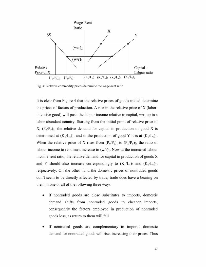
Fig. 4: Relative commodit

It is clear from Figure

the prices of factors o

intensive good) will p

labor-abundant count

X, (Px/Py)1, the relati

determined at (Kx/Lx)

When the relative pr

labour income to rent

income-rent ratio, the

and Y should also i

respectively. On the

don’t seem to be dire

them in one or all of t

• If nontraded

demand shift

consequently

goods lose, as

• If nontraded

demand for no

Wage-Rent Ratio

y prices determine the wage-rent ratio

4 that the relative prices of goods tr

f production. A rise in the relative pr

ush the labour income relative to cap

ry. Starting from the initial point of r

ve demand for capital in production

1, and in the production of good Y i

ice of X rises from (Px/Py)1 to (Px/P

must increase to (w/r)2. Now at the i

relative demand for capital in produc

ncrease correspondingly to (Kx/Lx)

other hand the domestic prices of n

ctly affected by trade; trade does ha

he following three ways.

goods are close substitutes to imp

s from nontraded goods to ch

the factors employed in production

return to them will fall.

goods are complementary to imp

ntraded goods will rise, increasing th

Capital-Labour ratio

SS

i

n

2

v

e

Y

X

(Ky/Ly)2

(Ky/Ly)1 (Kx/Lx)2 (Kx/Lx)1 (Px/Py)1

X

(Px/Py)2

(w/r)2

(w/r)1

Relative Price of

17

aded determine

ice of X (labor-

tal, w/r, up in a

elative price of

of good X is

t is at (Ky/Ly)1.

y)2, the ratio of

creased labour

tion of goods X

and (Ky/Ly)2,

ontraded goods

e a bearing on

orts, domestic

aper imports;

of nontraded

orts, domestic

eir prices. Thus

18

the factors employed in the production of nontraded goods will

gain as return to them will rise.

• If nontraded goods are neither substitutes nor complementary

goods to the imports, then there is no impact of trade on prices of

nontraded goods, thus no change in the return to their factors of

production is likely to take place.

Precisely, in light of the above described theoretical milieu, trade

liberalization would benefit the sectors that use the country’s most

abundant factor (labor in the case of Pakistan) intensively in their

production and harm those sectors that use the country’s scarcest factor

(capital in the case of Pakistan) intensively in their production or the

sectors that produce those nontraded goods that are close substitutes to any

of the imports.

Traditional Ricardian Theory suggested that only labor, as a single factor

of production, is needed to produce goods and services. Due to variation in

the technology across nations, the labor productivity is different among

different nations. It was this difference in the technology that initiated

advantages in producing specific goods and trading. Some goods or

industries are capital intensive if more capital per unit of labor relative to

other goods is used in their production or they have a higher capital-labor

ratio than other goods or industries in the country. Similarly, there are

goods or industries that are labor-intensive if more labor per unit of capital

relative to other goods is used in their production or these industries or

goods have a lower capital-labor ratio than other goods or industries.

19

2.3.2 Implications of the Model

Adjustments in national trade policy bring about changes in the prices of

goods (traded and nontraded) consumed domestically and in the labour

incomes11 of the workers. The impact of trade reforms comes from import

and export sectors.

In restricted trade regimes, prices of imported goods are kept higher than

the world price by imposing tariff and non-tariff barriers to trade. Liberal

trade policy may tend to increase the economic activity in the liberalized

sector as competition wipes out distortions from the market, paving the

way for efficient allocation of resources, trade liberalization on the other

hand may bring about losses for the local producers as they may lose their

share in the domestic market. Improved functioning of local markets due

to competition and less government intervention which helps in generating

new livelihood opportunities, reduces price and supply variability of

commodities, and eliminates market distortions

(monopolies/oligopolies/price administering, etc). Further, the imported

machinery, raw material, and advanced know-how may lead to enhanced

efficiency in the domestic production sector and increase the rewards to

the factors of production. Or, firms producing under the earlier protection

may lose hold of their previous market and embark on layoffs and

downward adjustments in the returns to their factors owing to the

competition. Similarly, the removal of trade barriers promotes export of

local products to the world market. The rise in exports cuts the existing

supply of a good in the local market tending to raise the domestic price.

Rise in the price of a good improves profit prospects for the business and

helps its expansion. The expansion of the producing unit results in higher

rewards for the workers of the unit. In the case of a developing country,

11 Wages and working hours

20

the returns to labor (wage) used intensively in the production sector would

rise, and returns to capital (rent) tend to fall.

In general, if liberalized trade policy affects the supply and thus reduces

the domestic prices of goods that are part of the consumption basket of the

poor in the country, the policy seems to benefit household welfare.

However, the fall in domestic prices of goods would in some ways affect

the labour incomes of the workers. Therefore it would be quiet unrealistic

to assess the impact of liberalized trade on poor household welfare just

from the information about change in the domestic prices. The realistic

assessment of the impact of trade on household welfare would consider

the cumulative impact of free trade on domestic prices and labour incomes

of workers.

2.4 Evidence from the Literature

For better organization and easy comprehension of the historical evidence

on the issue, the existing literature regarding trade effects on poverty via

factor and goods prices and household incomes in developing economies

is divided in two segments. The first segment consists of various studies

devoted to the impact of liberalized trade policies on wages of unskilled

workers in Latin American countries and the second studies the same, but

for Asian countries. Open trade experiences in the two regions have

encountered a situation of conflict of evidence. Latin American countries

suffered increased skilled-unskilled wage inequality and a rise in poverty,

and East Asian countries enjoyed a noticeable drop in wage differentials

leading to a reduction in poverty. The following sections present the

experience of Latin American and Asian countries’ trade policies.

21

2.4.1 Evidence from Latin America

Demonstrably, Latin American countries’ case is counted a failure of open

trade policy in light of the theoretical implications of the H-O model. The

reckoning stems from the fact that the skill premiums rose and inequality

and poverty worsened in these countries with the implementation of open

trade policies. During the late 1970s and 1990s many Latin American

countries (namely Costa Rica, Mexico, Chile, Colombia, Argentina, and

Uruguay) implemented an open trade policy by lowering tariffs and easing

quantitative restrictions on imports. Consequently, the skill differentials in

wages (identified at the levels of education) widened contrary to the

conventional wisdom of the H-O theorem12. The widening occurred from

the mid-1970s to the early 1980s in Argentina and Chile and between the

mid-1980s and the mid-1990s in Colombia, Costa Rica, and Uruguay. In

all cases, the relative number of skilled workers was rising, and thus the

dominant influence of the change in wages was a rise in skilled labor

demand. Time series calculations made by Wood, A. (1997) confirmed

that the relative demand for skilled workers rose during the liberalization

episodes in these countries. Skill differential in wages widened after the

mid-1980s in parallel with radical liberalization of the trade regime in

Mexico. Other studies have also explored the issue and confirmed the

presence of an association between wage inequality and open trade

policies in Latin American countries. Hanson and Harrison (1999)

estimated a trade-wage inequality link for Mexico and found evidence that

the skill-based wage differential was a consequence of removal of tariff

restrictions from the sectors that were relatively intensive in the use of

unskilled labor. The unskilled labor abundant sectors had shrunk and the

relative demand for skilled labor had shown a rising trend. They found

little variation in employment levels but a significant rise in skilled 12 For survey of literature on Latin American experience of trade liberalization and causes of widening gap between skilled and unskilled premiums see Wood, A. (1997), Chaudhuri, S. and Ghosh, A. (2001) and Robbins, D. J. and Gindling, T. H. (1999).

22

workers’ relative wages in Mexico. On the other hand they found no

correlation between the intensity of skilled labor and changes in relative

product prices, as suggested by the S-S model.

Robbins (1994, 1994a, 1996) and Feenstra and Hanson (1997) concluded

their analytical studies with similar results. Feenstra and Hanson (1997)

argued that the growth in foreign direct investment, which is positively

correlated with the relative demand for skilled labor, led to the higher skill

premiums in Mexico. Robbins (1994) found evidence of wage dispersion

in Chile between 1975 and 1990. He found a positive link between wage

differentials and the rise in the demand for skilled labor in Chile. Beyer et

al. (1999), using a time series approach, also found a long-term correlation

between openness and wage inequality in Chile.

Another study, [Chaudhuri, S. and Ghosh, A. (2001)] collected the

literature on the Latin American experience with open trade policies, and

the authors concluded their analysis with the important statement:

“removal of tariff restrictions from unskilled labour intensive sectors left

them unprotected which were highly protected previously and rise in

capital receptive foreign direct investment are the liable elements for

increase in the skill premium and wage differential as a logical outcome of

trade reforms.”

Additionally, Ianchovichina et al. (2001) used two-step procedures to

study Mexico’s potential unilateral tariff liberalization impact on Mexican

households. In first step they used Global Trade Analysis Project (GTAP)

model as the new price generator and in second step they applied the price

changes to Mexican households’ welfare. They concluded with a positive

effect of trade reforms on all income groups.

23

Without falling into a methodological controversy of evidence and

challenging the individual research work thereby, one may pose a serious

question here: Is it the liberal trade policy that intensified the skilled-

unskilled wage differentials or is something important missing from

consideration in the studies, for example the time of opening of the

economies and other methodological factors, affecting the findings. The

issue of conflict in evidence will be dealt with in the section on discussion

of empirical evidence. It is, though, difficult to develop a generalized point

of view on the impact of trade in favoring the unskilled production factors

in developing countries, but it is equally hard to ignore a consistent,

significant, and important factor of open policies resulting in a reduced

skill-unskilled wage gap in East Asian countries. The following section is

devoted for the East Asian experience with open trade policies.

2.4.2 Evidence from Asia

The evidence from so-called East Asian tigers (Hong Kong, the Republic

of Korea, Singapore, and Taiwan) on a trade-poverty link supports the

standard view of the H-O trade model, that the acceptance of more open

trade policies in developing countries with large numbers of unskilled

workers leads to increased demand for workers with a low level of skill

and education relative to the demand for highly skilled workers. The wage

gap between skilled and unskilled workers in South Korea and Taiwan

narrowed during the 1960s and in Singapore during the 1970s, and from

1973 to 1989 in Malaysia (Robins 1994a) after adoption of more open

trade policies. These countries had adopted open trade policies during the

1960s and 1970s and so gained the status of “early globalizers”. China,

though, joined the globalizers’ club during the early 1970s. Its rank

steadily rose from 30th largest trading country in 1977 to 3rd largest

importer (after EU and US) and 2nd largest exporter (after EU) in 2010

[WTO statistics 2010]. The most common aspect of these East Asian

24

newly industrializing countries is that they have been in the direction of

liberalization all along. There have been continuous unilateral trade policy

reforms in these countries away from high levels of protection previously.

However, Hong Kong and Singapore can be an exception in the group of

Asian emerging economies because they have been free port economies,

practicing zero import or export restrictions since the 1950s. These two

countries share a striking similarity with other East Asian Tigers that they

are at relatively the same level of economic development as each other.

Further, two more studies Fields (1994) and Robbins and Zveglich

(1995a) can be good sources for demonstrating the experience of these

four East Asian countries from open trade policies and poverty reduction.

Fields (1994) found that labor market conditions improved in all four

economies during the 1980s at rates on par with the rates of their

aggregate economic growth and that they grew without any repressions on

their labor markets during the same period. The four-country average rate

of growth in real per capita GNP is reported as 87.875% during the 1980-

90 decade, with a 89.57% growth rate in the real earnings of workers in

different sectors13. These East Asian newly industrialized economies

experienced a reduction in wage inequality after openness, with a strong

export-orientation introduced in the 1960s and 1970s. This was therefore

consistent with standard trade theory, which predicts that trade

liberalization should benefit the locally abundant factor (Wood, 1995,

1997; Krueger, 1983, 1990).

13 Hong Kong: Growth in real GDP per capita (64.2%): Earnings in manufacturing (60.0%); Korea: Growth in real GDP per capita (121.8%): Earnings in manufacturing and mining (115.8%); Singapore: Growth in real GDP per capita (77.5%): Earnings in all industries (79.8%); Taiwan (China): Growth in real GDP per capita (88.0%): Earnings in manufacturing (102.7%). Source: For Hong Kong: Government of Hong Kong (various years); for Korea: unpublished country data; for Singapore: Government of Singapore (1990); for Taiwan (China): Government of China (1991b). Also cited in Fields (1994).

25

2.5 Discussion on Empirical Evidence

The key implication of the difference in timing of embracing open trade

policy stems from the fact that by the time the Latin American countries

adopted open trade policy, they had lost the comparative advantage of

countries being rich in unskilled labor. Entry in the global market of four

heavily populated Asian countries—namely Bangladesh, China,

Indonesia, and Pakistan—with large numbers of unskilled workers by the

mid-1980s altered the position of Latin American countries in receiving

the comparative advantages from international trade. Although the ratio of

skilled to unskilled workers in those countries (Latin American) was still

far below that of the developed world, it was still above the global

average. This changed the basic principle of comparative advantage for

Latin American countries from the production of goods of low skill

intensity to goods of intermediate skill intensity. Additionally East Asian

countries opened up in the 1960s had already accumulated enough

skills/capital to shift their comparative advantage too from low to

intermediate intensity skills goods. Thus the greater openness in Latin

American countries during the 1980s instigated contraction of the sectors

both of high skill intensity goods (by imports from developed countries)

and of low skill intensity goods (by imports from low income newly

globalizing countries). The net effect might have been in either direction,

but greater openness could only result in an ever wider gap between

skilled and unskilled workers’ wages. The above explanation is supported

by Kaplinsky (1993), who attributed the losses in labor-intensive Latin

American manufacturing sectors to competition from imports from low-

income Asian countries domestically and in third-party market (for

example in the US, an important destination for Latin American

exports)14.

14 The main inspiration for the implications here is drawn from Wood, A. (1997).

26

Further, two more plausible explanations of the conflict of evidence on

trade liberalization experiences in the two regions have been explored in

Wood, A. (1997). The first implication is related to the increased global

demand for skills. Citing Robbins and Zveglich (1995a), Wood quotes the

global skill demand as the “Skill Enhancing Trade”. However, this

explanation is not ironclad, as the opening countries were not completely

cut off from new technology, yet, it is most likely that the countries

accumulate skills and alter their technological demand with increased

openness. East Asian countries can be presented as a reasonable case study

in this respect.

The second implication is associated with the difference between East

Asian and Latin American natural-resource endowments. In East Asia,

during the 1960s the majority of exports were concentrated in

manufacturing, whereas in Latin America trade gains were emanating

mainly from primary and processed primary exports, with manufacturing

exports often shrinking, except in the parts of Mexico adjacent to the

United States. This was because Latin America is far better endowed with

natural resources than East Asia and consequently had a comparative

advantage in production of primary products. Therefore the claims of

failure of liberal trade policies in Latin American countries may be refuted

with the rationale that it was not the trade reforms that raised skill

premiums but rather the increased global demand for technology, entry of

many labor-abundant countries in the world trade sector during the 1970s

and 1980s, and richness of the Latin American region in resource

endowments.

27

3 Choice of Methodological Technique

This Chapter opens the discussion on the choice of methodological

technique for the analytical structure of the present study. The previous

literature on the trade effects on various economic parameters

contemplates diverse methodologies that differ in a number of significant

ways. These analytical studies vary across dimensions, with analysis

carried out for representative households or actual households, employing

dynamic or static analysis, using single- or multi-regional statistics, and

using partial or general equilibrium approaches. Of these possibilities, four

main categories are identified as the important techniques, based on the

principal methodology applied [Reimer (2002)]. Each technique inherently

has certain limitations and degrees of complexity along with certain

advantages when applied for a variety of research objectives. The choice

of a suitable technique in a research study depends upon the desired

outcome and adherence to certain intrinsic conditions and limitations the

techniques are subject to. These conditions can be related to availability of

required quality data, accessibility to computing resources such as

computers with specific programs/softwares, and expertise required when

more complex and larger models are employed. Further, it is also crucial

to undertake the analysis of intended objectives before choosing any

methodology, whether the target is to measure the aggregated welfare

impact of a policy shock on the whole economy or is restricted to

exploring the relationship between a certain policy shock and a particular

variable. Since the conditions, scope, circumstances, and targets of

research projects vary in goals, so is the case with research techniques.

Hence, the preference for one research technique over others remains an

important area for authors and researchers as far as their own objectives

and goals are concerned. The principal methodological techniques

explored are Computable General Equilibrium Modeling technique, Partial

28

Equilibrium Analysis and Micro-simulation Modeling technique. Cross

country Regression Analytical Methodology would be out of the scope of

the present study since the present study is about working with national

data from a single country, Pakistan.

Thus the core discussion in this section encircles the merits and demerits

of the above three research techniques/methodologies. The purpose is to

justify the selection of one out of the three techniques, allowing realization

of the present study’s goals and advantages, limitations and conditions

embedded in the use of all three techniques individually.

The following descriptions of Partial and Computable General

Equilibrium are based on the textbooks of Black, Fischer (1996), Mas-

Colell, A., Whinston, M., and Green, J. (1995), and Varian, H. R. (2003).

For a detailed literature survey and categorization of studies by use of the

main research technique, refer to Reimer (2002).

3.1 Computable General Equilibrium (CGE) Analysis

This modeling technique represents a powerful tool used for

distinguishing the multiple economic effects on an economy surfacing

from various economic and trade policies. The CGE model addresses the

workings of an economy in an integrated manner by considering the

complex inter-linkages and feedbacks between production sectors,

households, and institutions.15

The following paragraphs will present an overview and the working of

General Equilibrium theory and model from the perspective of historical

and pioneering contributions by L. Walras (1834-1910), V. Pareto (1848-

15 For a brief history of General Equilibrium Modeling technique and a survey of its main contributions and application of the technique see Borges, Antonio M. (1986).

29

1923), F. Y. Edgeworth (1845-1926), and I. Fisher (1867-1947) in giving

the CGE technique its present modern shape. The fundamentals of the

CGE theory and model are provided by General Equilibrium theory,

which was introduced by French-born mathematical economist L. Walras

(1834-1910), a prominent marginalist and professor at University of

Lausanne, Switzerland, in his book Elements of Pure Economics published

in 1874. According to his theory, in a market system the prices and

production of all goods are interrelated. A change in the price of one good

is likely to alter the prices of other goods in the society. For example, a

small change in the price of bread may change the wages of the workers in

the bakery. Owing to these links between individual economic agents

(markets and households) in the economy, the theoretical calculation of

equilibrium price of just one good requires an analysis that accounts for all

of the various goods that are available in an economy.

Because the theory studies the behavior of individual agents in an

economy toward any policy changes and is capable of analyzing issues at

a micro level, this is distinguished as part of theoretical microeconomics

using a bottom-up approach (from analyzing links between individual

economic agents at the bottom to the whole economy at an aggregate

level). This microeconomic foundation of CGE specification guarantees

the simultaneous interaction among micro, market, and macro levels of the

economy that can capture all horizontal, vertical, and forward-backward

links among all production sectors, factors of production, and households

in the economy. See detailed account of theory of General equilibrium in

Kuenne, R. E. (1963).

The prevalence of perfect competition in the market is the key assumption

of General Equilibrium theory. Each decision-making unit in the economy

operates independently, i.e., each firm acts as if it were trying to maximize

its profits and every household acts as if it were trying to maximize its

utility. Thus the theory, in the market economy, seeks to find such a

30

unique solution where each unit of output is produced and sold at its

lowest unit cost in the quantity demanded by each household, given that

all markets are cleared. Assumption of perfect competition in the market

further suggests that each economic agent is a price taker and that all

prices are flexible. More precisely, the theory seeks to explain production,

consumption, and prices in a whole economy by coordinating the choices

of all economic agents across all goods and factor markets. Since all

markets are interdependent, simultaneous solution to the system implies

that, as mentioned above, the price of any one good will be affected by a

change in the price of the other good. In addition, by virtue of production

and market theories, it is assumed that the system is homogenous of

degree zero in absolute prices: if the values of all price variables are

increased equi-proportionately, the values of the quantity variables will be

left unchanged. The main issue, thus, is the existence of equilibrium in all

sectors of the economy. That is, even though it could be demonstrated how

individual markets behaved, it would remain unknown how goods

interacted with each other to affect supplies and demands in multiple

markets in the absence of a simultaneous solution for all markets.

While working on his book Elements of Pure Economics (1874) Walras

presented his idea of equilibrium by conceiving the prevalence of

consistency in the equilibrium concept in terms of the number of equations

required for market clearing and the number of variables available to

obtain it: the prices [Carvajal, A. (2006)16]. To solve this problem, he

created a system of simultaneous market demand and supply equations.

Studies using Computable General Equilibrium modeling technique

account for commodity market and terms of trade, and factor market

effects by using disaggregated Social Accounting Matrix (SAM) as an

analytical base. Several studies have been conducted using CGE modeling

16 p1

31

technique to measure the trade effects on poverty and welfare in

developing countries. Some of these studies include Coxhead and Warr

(1995), who examined the impact of technical progress in agriculture on

changes in poverty and aggregate welfare in Philippines. Loefgren (1999)

analyzed the short run equilibrium effects of reduced protection in

agriculture sector using GE model and found that the reduced agricultural

protection would generate significant aggregate welfare gains. Cogneau

and Robilliard (2000) used general equilibrium framework to examine the

impact of various growth strategies on poverty and inequality prospects in

Madagascar. Sadoulet and De Janvrry (1992), have pursued a multimarket

approach for analyzing the impact of trade liberalization on the agriculture

sector in Africa using General Equilibrium approach. Harrison,

Rutherford, and Tarr (2001) explored the case of trade liberalization and

poverty in Turkey using CGE model with 40 households distinguished by

income levels and urban or rural locations. Evans (2001) worked to

investigate the impact of global trade policy reform on South Africa by

integrating the findings from GTAP and poverty case studies for Zambia.

He found that the unilateral trade reforms improved income but were

having strong bias towards metropolitan areas against poor rural sectors.

Limitations and Advantages

Traditionally, for three obvious reasons, the study of General Equilibrium

analysis has been emphasized: first, it studies the essential duality of

pricing and resource allocation; second, it represents the interdependence

of different parts of an economic system; and third, it provides a unifying

framework within which some major branches of economic theory such as

the theory of value, welfare economics, pure theory of international trade,

and the theory of economic growth can be shown as having a common

32

origin, since all have the common goal of determining the price of goods

and services and efficient allocation of resources [Simpson, D. (1975)17].

Though theoretical superiority of Computable General Equilibrium system

has remained unchallenged, nevertheless some studies have argued that

analytically it is not a useful exercise and found it limited to merely the

description of numbers and data without giving a concrete basis for policy

making. Borges, A. M. (1986) concludes that CGE models happen to be

significantly large, comprise substantial parameters, and often embody

complex structures. Parameters incorporated into the model are not

estimated econometrically; rather, they are estimated independently out of

the model and are then calibrated to a single data point, which is chosen to

represent a situation close to general equilibrium [Borges, A. M. (1986)18].

Thus the exercise of parameters being isolated from the main model leaves

the results of the model not to forecast the reality but rather only to

indicate long-term tendencies around which the economy will fluctuate.

Due to that fact, results from CGE modeling can neither be useful for

replication of the evolution of the economy in the past as a means of

checking their validity nor can be applied for future policy making. This

feature of CGE modeling defeats the inherent purpose of the research, i.e.,

performing efficient future policy making based on concrete estimations,

results, and evaluating the previous policies by using trade models.

Its strengths include its coherent microeconomic theoretical foundation,

internal consistency, suitability for policy issues involving substantial

changes in variables’ absolute and relative terms, and its concern to

measuring welfare loss or gain of the whole economy. But these are

merely theoretical advantages, since we could never include every aspect

of the world economy in a mathematical model, nor could we quantify

every step of certain policy implementation precisely in any computer

17 p 9 18 p 19

33

simulation model. Therefore, performing CGE exercises without

econometrically estimating the coefficients and parameters is nothing

more than scientifically pretending to cover all of the linkages and

feedbacks from the whole economy in the analysis, while the reality

happens to be far from it.

3.2 Partial Equilibrium Analysis

Partial Equilibrium Analysis is a way of obtaining an estimate of the

impact of a change in the economy that does not require the complete

solution of the General Equilibrium system [Whalley (1974]. It is another

view of measuring and establishing the link between variables (for

example, trade and poverty) in the economy. A Partial Equilibrium view

in the context of trade is considered a part of the General Equilibrium

analysis, where the clearance of the market of some specific goods is

obtained independently from prices and quantities demanded and supplied

of other goods' markets. Unlike CGE models with an aggregate behavior,

Partial Equilibrium models of trade do not give an aggregate view of the

welfare of an economy; rather, they allow researchers to focus on how the

gains and losses from a shift to free trade are shared across specific

individuals/households and markets in a more detailed and reliable way.

The argument can also be put this way: It is a way of obtaining an estimate

of the impact of a change in the economy without requiring the

simultaneous solution of the whole economic system. The impact of real-

world policy options on any specific sector is investigated, keeping other

things constant under ceteris paribus assumptions. Quoting the trade-

poverty link here, one can assert that the investigation of the impact of

trade policy on a specific sector is established through disseminating the

straightforward way of measuring welfare effects of international trade

34

through estimating changes in consumer surplus, so that consumer welfare

can be measured.

This type of analysis either ignores effects of the policy in other industries

in the economy or assumes that the sector in question is very small and

therefore has little, if any, impact on other sectors of the economy.

Whaley (1974) classified Partial Equilibrium Analysis into simple and

extended versions. According to him, under Simple Partial Equilibrium

Analysis, all prices and quantities except of the commodity under

consideration are treated as constant and non-variant with time.

Additionally, linearization assumptions are employed as local

approximations to ease the problem of computing new estimates after

policy implementation. This is also known as the log linear version of the

system, due to its linearity assumption. However, he reckons it an

Extended Partial Equilibrium Analysis when the linearization assumptions

are relaxed and the impact of the change of a single price (when allowed

to vary) upon the value of the demand for other goods via changes in the

value of endowments is incorporated inside the system environment. This

nonlinear version of the system can be solved through linear

approximation methods [Borges, A. M. (1986)].

Partial Equilibrium technique is deemed useful in studies that focus on

specific and straightforward relationships between variables with strong

precision for future policy making. Use of this technique can help

overcome various research-related issues, such as availability of large

accurate and reliable data.

There are ample studies using Partial Equilibrium modeling approaches.

By using household expenditure data, these studies generally emphasize

commodity markets and their role in determining poverty impacts as a

measure of poverty across time. The studies reviewed here using this

approach are Appleton (2001), Fofack, Célestin, and Tuluy (2001), Deaton

35

(1989), Dercon (2001), Ravallion (2004), Ravallion and Van de Walle

(1991), Levy and van W. (1992), McCuloch and Calandrino (2001), Case

(1999), Levinsohn, Berry, and Friedman (1999) and Minot and Blauch

(2002).

Limitations and Advantages

Some macro-level studies using Partial Equilibrium technique divulge the

inability of this technique to precisely measure the terms of trade effects

for each region and assess their income distributional consequences across

regions and socioeconomic groups within regions [Harding, Ann

(2007)19]. Partial Equilibrium technique has limited ability to assess

second-order effects (inter-industry effects and macroeconomic

adjustments that often appear to be significant) of a policy. However,

Partial Equilibrium technique is preferred when the sector under study is

only part of a whole, so the generated effect claims are exclusively and

precisely for that specific part of the whole. Further, the technique is

efficient when the shock from a policy change to be measured on a sector

has limited backward and forward linkages with other sectors of the

economy.

It focuses on only part of the economy at a time, overlooking interaction

between various markets in order to overcome the complexities (arising

from limited availability of accurate data and use of complicated computer

programs, for instance) and ensuring simplicity, straightforwardness, and

transparency in analysis owing to its reliance on few key parameters. The

above arguments are considered as the benefits of this system, rendering it

preferable to Computable General Equilibrium technique. The partial

19 p5

36

system is more reliable and authentic vis-à-vis its usefulness in future

policy-making and evaluation of trends in past policies.

The present study uses fairly long time series data of 36 years for demand

estimation and 14 years data on tariff to investigate and estimate the links

between prices, labour incomes, and poverty to analyze past trends and

perform future forecasting. Since all relationships between various

parameters are econometrically estimated therefore, results derived under

Partial Equilibrium analysis are trusted for future forecasting and policy

making, since they are more reliable and straightforward than those

derived from Computable General Equilibrium model.

3.3 Micro Macro (Simulation) Models

The need for spatially disaggregated data gave birth to this technique.

Spatially disaggregated data can be extremely useful for regional and

social policy analysis, as it presents efficient representation of individuals.

It is a technique used to model complex real life events by simulating the

impact of policy change (characteristics and behavior) on individual units

of the whole system wherein the changes occur. It has generally been

accepted as a valuable policy tool used to analyze the detailed

distributional and aggregate effects of both existing and proposed policies

at a micro level, where individual households are taken into account to

capture individual heterogeneity. Pioneering work on micro simulation

was conducted by Orcutt (1957)20.

In the modern world, researchers and policy makers attempt to achieve

multiple social policy objectives such as income redistribution, ensuring

access to health and education, and a reasonable standard of living for

most of the citizens. Most researchers prefer solo microsimulation models

20 Also cited in Merz, J. (1995)

37

to assess distributional effects of public policies with no possibility to

analyze the efficiency impact of the policy. Others prefer macro models to

measure the efficiency of the policies while ignoring the distributional

effects. Given the emphasis on changes in income distribution,

microsimulation models are often used to investigate the impacts on social

equity of fiscal and demographic changes (and their interactions).

Modeling of the distribution of traffic flows, for example over a street

network, is another increasingly important use of the approach21.

For the purpose of distributional analysis of micro data, micro simulation

models are integrated with macro models. These models/links can serve

the dual purpose of computing efficiency impacts and conducting

distribution analysis using micro data. Two approaches have been

identified in incorporating micro data into a macro model: Integrated

Microsimulation models and Micro-Macro models. Integrated

Microsimulation models attempt to incorporate individual household

information generally found in income-and-expenditure-based household

surveys into macro frameworks. Data for these models comes in the form

of disaggregated SAM account. The labor- and wage-based income

generation of different households is categorized according to various

occupations in industrial sectors, profit income, government transfers, rest

of the world transfers and other income. A Micro-Macro approach follows

mainly sequential linking of a model based on micro-level data with a

model based primarily on macro-level data [Reimer (2002)]. The key

studies that use this technique are Ianchovichina, Nicita, and Soloaga

(2001), Cockburn, J. (2001) and Robilliard, Bourguignon, and Robinson

(2001). The models are then linked by modifying selected parameters of

the Microsimulation model according to certain variables generated by the

macro model.

21The International Microsimulation Association descriptions

38

Microsimulation model is used to replicate microeconomic features of a

labor market as well as household consumption and income behavior from

household data sets, while a macro model generates values for macro

variables such as total employment, prices of commodities, and wages,

etc. Finally the Microsimulation model is solved in such a way that results

are consistent with the aggregated variables generated by the macro

model. This is different from the previous microsimulation approach in

several ways. In the earlier method, the process of disaggregating

individual households from the household sector captured micro-level

issues, whereas in this approach a separate model is developed

encompassing other socio-economic and demographic features to capture

the interactions explicitly.

Limitations and Advantages

Comprehensive data linkage, spatial flexibility, and the ability to update

existing data and forecast for the future are some of the advantages of

Micro-Macro modeling technique. However, its disadvantages, such as

difficulties in calibrating the model and validating the model outputs

sometimes even overshadow its advantages.

3.4 Choice of an appropriate Modeling Technique

The goal of the study is to provide reliable econometrically estimated

results from a long time series of 36 years data for the demand estimation

and 14 year data for measuring the price effects and change in labour

income in agriculture and manufacturing, which can be used for future

forecasting and analyzing past trends regarding the link between trade and

39

poverty in Pakistan. The nature of the study in hand requires

accomplishment of a two-fold goal. First, establishment of the link

between reduced import duties (trade openness) on poverty in the country

via tracing changes in labour income in the selected sectors and prices of

selected traded and nontraded goods consumed by the poorest households

in Pakistan. Second, generation of econometrically tested welfare

estimates that can be used for future policy making as well as have the

capability to explicate past trends. Use of Partial Equilibrium approach

(with support of general equilibrium framework) in the study seemingly

discharges the two-fold goal in a more efficient way than the CGE and

Micro-Macro techniques. The following points support the preference of

Partial Equilibrium technique over other techniques.

1. The present study is about analyzing the long time series data of 36

years to estimate demands and 14 years time series to estimate the

welfare measures and change in the labour income in agriculture

and manufacturing, and CGE modeling technique does not provide

the empirical validation since there is no measure of the degree to

which a model can fit the data or can track historical facts. Owing

to the unrealistic assumption of prevalence of equilibrium in all

markets, the CGE technique is inappropriate to be used for

forecasting the reality; rather, it can only indicate the long-term

tendencies around which the economy will fluctuate.

2. Partial Equilibrium technique is preferred for its simplicity since it

does not call for developing complex structures based on

accounting and input-output matrices that are needed in General

Equilibrium technique to obtain the required results. Since the

research is devoted to the enquiry of links between specific

variables in a part, rather than the whole, i.e., the link between

trade policy changes and changes in labour incomes and prices.

Partial Equilibrium modeling technique, thus, suits the study most

40

as it produces estimated results usable for future policy forecasting

and evaluating past trends.

3. Again, the purpose of the study is not to measure the terms of trade

effects for each region and assessment of income distributional

consequences across regions and socioeconomic groups within

regions, where Partial Equilibrium has some limitations and

General Equilibrium technique has an edge over Partial

Equilibrium technique. Yet, the limitations of Partial Equilibrium

technique in this specific realm would not hamper the realization

of the goals of the present study.

4. The estimation of second order effects of trade policy across the

economy is out of the scope of the study. So use of Partial

Equilibrium technique would still have no bar on attainment of the

objectives of the study. Though General Equilibrium modeling

technique is more suitable while considering second order effects,

the General Equilibrium results are not econometrically estimated

and so not reliable for future policy making and forecasting.

Therefore, Partial Equilibrium modeling technique seems more reasonable

and reliable since the feature of General Equilibrium technique to carry

parameters into the model that are not estimated econometrically, rather

are estimated independently out of the model and are then calibrated to a

single data point, which is chosen to represent a General Equilibrium

situation, limits its capability to be used for future policy making and

analyzing past trends. Further, the use of a Micro-Macro technique would

be more complex and cumbersome than necessary for the present study

[Borges, A M. (1986)].

41

4 Trade Liberalization, Prices of Traded and Nontraded Goods, Households’ Labour Income, Welfare, and Poverty

The idea here is to investigate the distributional effects of trade reforms

and a selective protectionist trade policy in some commodity groups on

the welfare of the poorest households in Pakistan via changes in domestic

prices and labour income using household and labour force data in partial

equilibrium setting22. The approach is based on the specifications of Porto

(2003, 2006), however some of its methodological inaccuracies are also

pointed out and corrected in the present study. Porto (2003) implicitly

assumed that there are no quantity effects of a trade liberalization induced

price change. That would imply that the households’ demand curves for all

selected goods are vertically sloped which is against the conventional

demand theory. Secondly, Porto has estimated the domestic prices on the

international prices and the tariff rates treating implicitly the tariff rates as

a variable determined in the system whereas on the contrary the tariff rates

are fixed by the government so are exogenously given like the

international prices. In present study these failings have been corrected by

first considering the quantity effects by allowing the quantities demanded

of the selected goods to change with a change in the domestic prices.

Second, the domestic prices are not estimated instead they are calculated

by adding the tariff per ton to the international prices. The following

analysis begins when a change in the trade policy, treated as an

exogenously determined variable, brings about a change in domestic

prices of traded goods. This change in domestic prices further entails a

multitude of other impacts in the small open economy, including a change

in the domestic prices of nontraded goods and the labour income. The

22 For review of the studies examining the trade liberalization effects using household data in partial equilibrium see Attanasio, O., et al., (2004) and Deaton, A. (1989).

42

variations in domestic prices and the adjustment in labour income23 lead to

a change in households’ welfare.

The present Chapter is organized in two parts. The first part is about the

modeling of some basic interrelations between trade policy, domestic

prices and factor prices. The second part of the Chapter includes the links

between trade policy, households’ demands and welfare effects. The

welfare effects of a change in the trade policy are captured by measuring

the change in Marshallian Household Consumer Surplus. The Marshallian

Household Consumer Surplus is then corrected by deducing the income

effect from the total price effect using the slutsky equation to measure the

Hicksian Compensating Variation. Further, the change in labour income of

agriculture and manufacturing workers resulting from the change in the

trade policy is measured. The change in the poorest households’ welfare is

measured using Marshallian Consumer Surplus approach.

4.1 Interrelations between International Trade, Domestic Prices, and

Factor Prices

4.1.1 Domestic Prices of Traded Goods

Since the price variations accounted for are trade and tariff driven, it

would be interesting to know how domestic prices of traded and nontraded

goods are determined in the local market when the tariff rate changes.

Pakistan, being an economically small developing country, plays the role

of a price taker in the global trade sector. Thus in analogy with other small

open economies, the determination of domestic prices of traded goods in

Pakistan would look as follows:

23 Wage rate times the working hours

43

i wi iP=P (1+t ) (1)

Here Pi and Pwi are the domestic and world prices of the traded goods i

respectively, and ti is the rate of tariff applied on traded goods. If the

international price is exogenously determined, then the change in the local

price would be established by the given change in the rate of tariff (which

is also exogenously determined as it is fixed by the government). This is

shown in the following set of equations.

)t(1P)t(1PPPdPi i1wii2wii1i2 +−+=−=

or

)(tPPPPdP i1i2wii1i2i −=−= (2)

or

iwii dtPdP = (3)

It can be inferred from equation (3) that given exogenous world price, the

absolute change in the domestic price depends upon the international price

times the tariff change. Taking log on both sides in the equation (3) we

will have;

)t(1dlnPdlnP iwi += (4)

For simplicity reasons, here we would allow the relaxation of two strong

assumptions. Firstly, there are unified products and one tariff line for

imports of the same product for all countries. In this way, we are indeed

relaxing the Armington assumption [Lloyd, J. P. et al. (2006)] of

differentiated products with respect to their various points of origin or

production (countries). Secondly, it is further assumed that the goods have

similar prices throughout the whole country. Though, in developing

countries, this assumption may not hold in its entirety for a variety of

reasons such as irregular market structures, information unevenness, etc.

44

Nevertheless, in the case of Pakistan, owing to sea access and a relative

good communication and transportation infrastructure, as well as

developed markets in urban sectors, equation (4) can be a reliable exercise

to determine the absolute price changes caused by a change in tariff.

4.1.2 Domestic Prices of Nontraded Goods

As we already have learnt from the S-S findings, the prices of traded

goods are dependent upon factor price (wage)24:

)(wfP iii = (5)

This means that if the factor prices can be derived from the prices of

traded goods, they in turn uniquely determine the prices of nontraded

goods. In this case, prices of nontraded goods are independent of demand

conditions or factor supply. They only depend on technology and the cost

of input factors. Thus, in general equilibrium, an aggregate relationship

between prices of traded and nontraded goods can be established in the

form of:

)f(PP TNT =

Here PNT are prices of nontraded goods and PT are prices of traded goods.

The above relationship between prices of traded and nontraded goods can

be specifically expressed in following way:

T

NTTNT lnP

lnP.dlnPdlnP∂∂

= (6)

The equation 6 captures the change in the domestic prices of nontraded

goods by the multiplying the elasticity of prices of nontraded goods with 24 Also proved in section 4.1.3, see equation 19

45

respect to traded goods T

NT

lnPlnP∂∂

with the percentage change in the prices of

traded goods TdlnP .

4.1.3 Households’ Labour Income

At this point we are ready to establish a link between trade reform-induced

price change and the change in households’ labour income via the impact

of a price change on wages and working hours. To begin with, it is shown

that households’ labour income is determined from the information on the

prevailing working hours and the wage of the labor. It can be written as:

wLYi = (7)

Here w stands for wage per hour, L stands for labor hours, and Yi is the

total labour income of household i. This section mainly follows the

theoretical foundations of International Trade Theory provided in

advanced textbooks of Dixit and Norman (1980) and Woodland (1982).

The discussion on the impact of changes in the prices of traded goods on

wage with Cobb Douglas Production Function is opened here. Cobb-

Douglas Production Function is used in the whole study, having constant

returns to scale where the market is dominated by a large number of

buyers and sellers.

βαKLQ = (8)

As per the assumption of the constant returns to scale, the Cobb-Douglas

Production Function as shown in equation 8 assumes: α + β=1. To find out

the average cost we would begin with the total cost function, which is

given as:

rKwLTC += (9)

46

Here TC stands for Total Cost, w stands for wage, r stands for capital rent

and K stands for capital.

The assumption of constant returns to scale further implies two

propositions:

Increasing the two input factors (labor and capital) by λ would result in

output supplemented by the same amount, i.e., λ

λQQλKLλλKλLλλKλL βαβαβαββααβα ==== + (10)

Similarly the total cost would rise by the same amount:

T C = w λ L + rλ K = λ (w L + rK )= λ T C (11)

The average cost function can be derived from the production function (8),

retaining the minimal cost combination. The minimal cost combination

requires equality between the Marginal Rate of Technical Substitution

(MRTS) and the ratio of factor prices (wage and capital rent) wMRTS=r

,

where MRTS is the amount by which the quantity of one input is to be

reduced, when one extra unit of another factor is used, so that the output

remains constant. According to the firm theory, the MRTS is the ratio of

values of the marginal productivities of two factor inputs (capital and

labor). Thus we have:

LQ

MPL ∂∂

=

Marginal Labor Productivity

KQ

MPK ∂∂

=

Marginal Capital Productivity

rw

==

∂∂∂∂

−

−

α1β

β1α

LβKKαL

KQLQ

(12)

Solving equations for labor (L) and capital (K), we have:

47

= +

βα

rw

QL α11

(13)

= +

βα

wr

QK β11

(14)

After inserting results from (13) and (14), we can derive Total Cost

function under the conditions of perfect competition.

+

=

αβ

βα

βα

βα

rwQTC (15)

The Average Cost function, thus, is as follows:

+

=

αβ

βα

βα

βα

rwQ

TCAC (16)

After close observation of the relationship in (16), one can find that the

average cost is a function of the factor prices and a constant

+

αβ

βα

βα

made up of production elasticities of labor and capital.

Further, it should also be noted that the average cost does not depend upon

the level of output Q, since in perfect competition there is no profit margin

and the price is equal to average cost. Therefore:

(K)rwP βα= (17)

Or transformed to linearity and ignoring the constant (K), we have;

βlnrαlnwlnP += (18)

The relation between factor and goods’ prices expressed in (18) can also

be put in more general terms:

48

r)(w,fP ii = (19)

Equation (19) confirms that commodity prices Pi are the function of factor

prices w and r. Since our main focus here is to determine the link between

factor price and commodity price in a developing country setting with a

labor intensive production sector, the role of capital is ignored.

In equation (19), Pi is the vector of commodity prices, fi is the average

cost function, (since in perfect competition there is no profit margin and

price is equal to average cost) and w and r are the vectors of factor prices

(wage and capital rent). From this model, it is attempted to show that the

prices of goods are determined from the set of wages. Nevertheless, the

main objective is to know: Can wage be uniquely determined from

information on commodity prices, i.e., )( pfw j = ? Here rises the

question of invertibility. To resolve the issue of invertibility (univalence),

the 2x2x2 H-O model is referred. From 2x2x2 H-O model, one knows that

the commodity price vector has the ability to determine the factor price

vector as long as there is no issue of Factor Intensity Reversal25. This, in

other words, means that factor prices do not depend upon factor

endowments and are also not affected by any variability in it. The

relationship between commodity prices and factor prices in this specific

fashion has been called as Factor Price Insensitivity26 in the literature. This

can simply be illustrated by mapping the average cost functions in a factor

price diagram as shown in the following two graphs of Figure 5.

25 Factor Intensity Reversals is a property of the technologies for two industries such that the ordering of relative factor intensities is different at different prices. 26 Leamer (1995) has emphasized that a sufficiently diversified small open economy has a national labor demand that is infinitely elastic. Also quoted in Slaughter (2001).

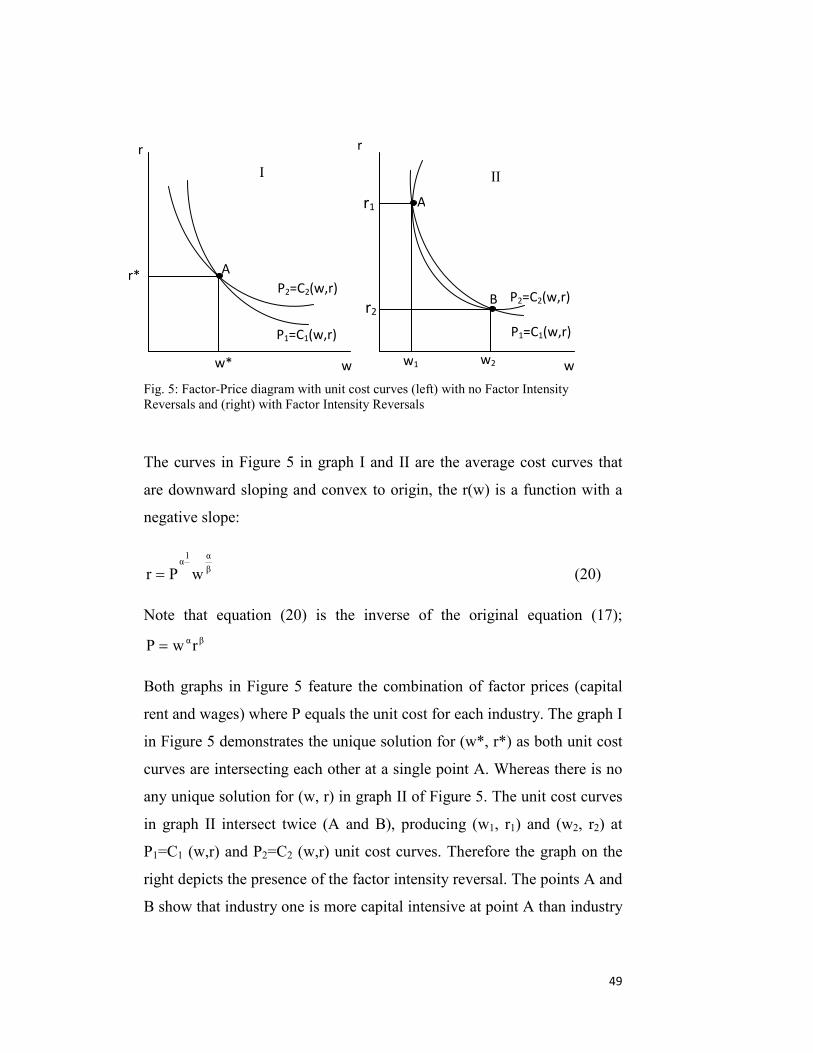
Fig. 5: Factor-Price diagram with unit Reversals and (right) with Factor Inten

The curves in Figure 5 in graph

are downward sloping and conv

negative slope:

βα1

α

wPr =

Note that equation (20) is thβαrwP =

Both graphs in Figure 5 feature

rent and wages) where P equals

in Figure 5 demonstrates the un

curves are intersecting each oth

any unique solution for (w, r) in

in graph II intersect twice (A a

P1=C1 (w,r) and P2=C2 (w,r) un

right depicts the presence of the

B show that industry one is mor

r

cost curves (left) with no Factor Intenssity Reversals

I and II are the average cost c

ex to origin, the r(w) is a funct

e inverse of the original equa

the combination of factor pric

the unit cost for each industry. T

ique solution for (w*, r*) as bot

er at a single point A. Whereas

graph II of Figure 5. The unit c

nd B), producing (w1, r1) and

it cost curves. Therefore the gr

factor intensity reversal. The po

e capital intensive at point A tha

w

w

II

I

r2

r r1

P2=C2(w,r)

P1=C1(w,r)

P2=C2(w,r)

P1=C1(w,r)

B

A

w1

w2 w*

A

r*

r

49

ity

urves that

ion with a

(20)

tion (17);

es (capital

he graph I

h unit cost

there is no

ost curves

(w2, r2) at

aph on the

ints A and

n industry

50

two and more labor intensive at point B27. This means that the ordering of

the relative factor intensities is different at different prices. The

determination of the unique solution (for w and r) depends upon the unit

cost curves intersecting each other only once. This is true when the two

unit cost curves portray the same curvature (same value for the

substitution elasticity of production factors). If the substitution elasticity

between two industries differs, hence the curvature of the unit cost curves

also differs, and the unit costs curves necessarily intersect twice (or none).

If both industries exhibit Cobb-Douglas type production functions, they

intersect only once, since both have the substitution elasticity of 1. In

absence of factor intensity reversal, the change in the commodity price

will cause a change in the factor price. With a rise in the commodity price,

the real return to the factor used intensively in its production will rise,

while the return to the other factor will fall. This reflects the core of the

famous S-S theorem.

Further, the above example of Cobb-Douglas Production Function can be

referred back to in the following way. Taking the total differential of price

equation (17) and dividing by P would provide the percentage change in

goods and factor prices.

βα

1βα

βα

β1α

rwdrrβw

rwdwrαw

PdP −−

+=

or

rdr

βw

dwα

PdP

+= (21)

To grasp the connotation more clearly, the equation (21) can be broken up

into three parts: P

dPis the percentage change in the prices of commodities,

27 See Feenstra (2004) for detailed explanation of reversals of factor intensities between two industries.

51

wdw

is the percentage change in the wages of workers, and r

dr is the

percentage change in the rent of the capital. Parameters α and β provide

the weights of wage and capital rent (of percentage change in wage and

percentage change in capital rent respectively) that the wage and capital

rent has on the price change of a good. In other words, they define the cost

shares that each factor has in production.

Denoting the percentage change by hat ^, the equation can be rewritten for

the two-good two-factor case as follows:

^

1

^

1

^

1 rβwαP += (22)

^

2

^

2

^

2 rβwαP += (23)

After solving the above two equations for ^r and

^w and arranging them in

matrix form, we can receive it as follows:

−

−=

⇒

=

^

2

^

1

12

12

^

^

^

^

22

11

^

2

^

1

P

P

αα

ββ

D1

r

w

r

w

βα

βα

P

P (24)

Where D denotes the determinant of the matrix on the left, which is

defined as:

212112212121 ββαα)α(1α)α(1ααββαD −=−=−−−=−= (25)

Equation (25) is true after referring to the assumption of Constant Returns

to Scale, where 1βα ii =+

To facilitate the solution of the matrix for wages (w) and capital rent (r),

the determinant has been taken as inverse of the matrix.

To analyze the goods’ price changes, we assume first that the industry I is

more labor intensive and secondly that the price of good 1 rises after trade

52

reforms. As per first assumption we have the value of

0ββααD 1221 >−=−= and secondly, 0PP^

2

^

1 >− . By using the above

information, we can solve for the changes in factor prices. Multiplication

of column vector of percentage change in prices of two goods

^

2

^

1

P

Pwith

the inverse matrix

−

−

12

12

αα

ββ will solve the matrix for impact on wages

(percentage change) and capital rent (percentage change). Consequently,

the labor wage and capital rent equations would appear as follows:

Wage equation:

−=^

21

^

12

^

PβPβD1

w (26)

Without affecting the uniqueness of equation (26) and the results thereby,

we have arbitrarily adjusted the parameters (α, β) and price vector (^ ^

1 2P , P )

in (26a) and (26b) for wages and (27a) and (27b) for the capital rent:

−+−= )PP(β)β(βPD1

w^

2

^

1112

^

1

^

(26a)

or

( )( ) ( )

>−

−+

−−

=^

1

^

2

^

112

1^

112

12^

P)PP(ββ

βP

ββββ

w (26b)

Capital rent equation

−=^

12

^

21

^

PαPαD1

r (27)

−−−=^

2

^

1221

^

2

^

PP(α)α(αPD1

r (27a)

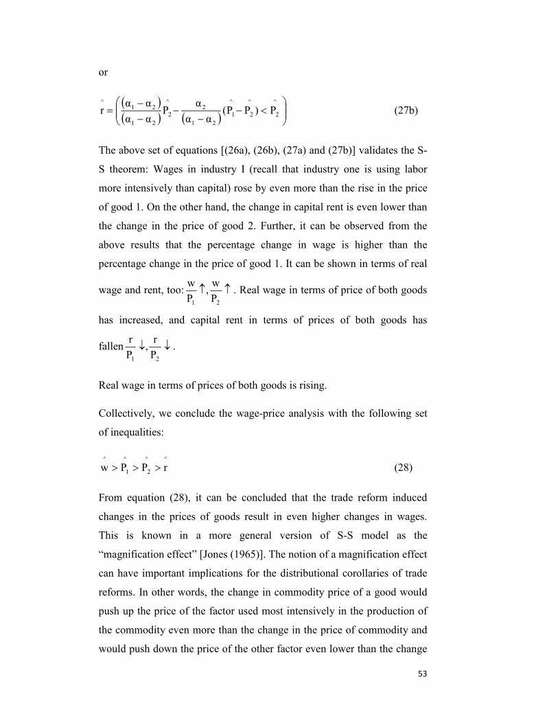
53

or

( )( ) ( )

<−

−−

−−

=^

2

^

2

^

121

2^

221

21^

P)PP(αα

αP

αααα

r (27b)

The above set of equations [(26a), (26b), (27a) and (27b)] validates the S-

S theorem: Wages in industry I (recall that industry one is using labor

more intensively than capital) rose by even more than the rise in the price

of good 1. On the other hand, the change in capital rent is even lower than

the change in the price of good 2. Further, it can be observed from the

above results that the percentage change in wage is higher than the

percentage change in the price of good 1. It can be shown in terms of real

wage and rent, too: ↑↑21 P

w,

Pw

. Real wage in terms of price of both goods

has increased, and capital rent in terms of prices of both goods has

fallen ↓↓21 Pr

,Pr

.

Real wage in terms of prices of both goods is rising.

Collectively, we conclude the wage-price analysis with the following set

of inequalities:

^^

2

^

1

^

rPPw >>> (28)

From equation (28), it can be concluded that the trade reform induced

changes in the prices of goods result in even higher changes in wages.

This is known in a more general version of S-S model as the

“magnification effect” [Jones (1965)]. The notion of a magnification effect

can have important implications for the distributional corollaries of trade

reforms. In other words, the change in commodity price of a good would

push up the price of the factor used most intensively in the production of

the commodity even more than the change in the price of commodity and

would push down the price of the other factor even lower than the change

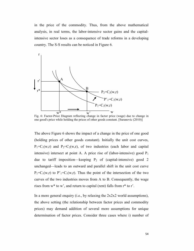
r*

in the price of the commodity. Thus, from the above mathematical

analysis, in real terms, the labor-intensive sector gains and the capital-

intensive sector loses as a consequence of trade reforms in a developing

country. The S-S results can be noticed in Figure 6.

Fig. 6: Factor-P reflectinone good's price while holding the prices of other g

The above Figure 6 shows the impact of a

(holding prices of other goods constant)

P1=C1(w,r) and P2=C2(w,r), of two indu

intensive) intersect at point A. A price ri

due to tariff imposition—keeping P2

unchanged—leads to an outward and par

P1=C1(w,r) to P’1=C1(w,r). Thus the poin

curves of the two industries moves from A

rises from w* to w’, and return to capital (

In a more general enquiry (i.e., by relaxing

the above setting (the relationship betwee

prices) may demand addition of several

determination of factor prices. Consider

P2=C2(w,r)

r

factor oods co

chang

. Initia

stries

se of

of (c

allel sh

t of th

to B

rent) fa

the 2

n fact

more

three c

w

price (wage) due to change in

w’ g change in

w* rice Diagram

r’

P1=C1(w,r)

P’1=C1(w,r)

A

B

54

nstant. [Suranovic (2010)]

e in the price of one good

lly the unit cost curves,

(each labor and capital

(labor-intensive) good P1

apital-intensive) good 2

ift in the unit cost curve

e intersection of the two

. Consequently, the wage

lls from r* to r’.

x2x2 world assumptions),

or prices and commodity

assumptions for unique

ases where i) number of

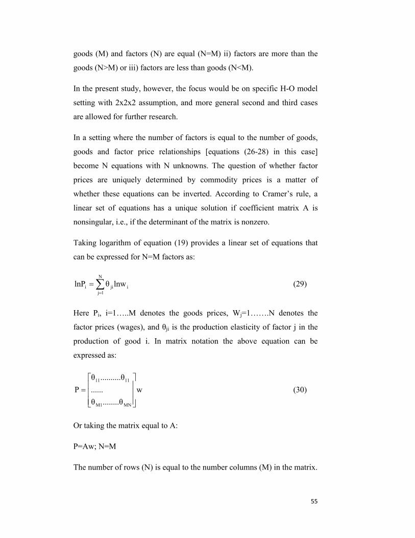
55

goods (M) and factors (N) are equal (N=M) ii) factors are more than the

goods (N>M) or iii) factors are less than goods (N<M).

In the present study, however, the focus would be on specific H-O model

setting with 2x2x2 assumption, and more general second and third cases

are allowed for further research.

In a setting where the number of factors is equal to the number of goods,

goods and factor price relationships [equations (26-28) in this case]

become N equations with N unknowns. The question of whether factor

prices are uniquely determined by commodity prices is a matter of

whether these equations can be inverted. According to Cramer’s rule, a

linear set of equations has a unique solution if coefficient matrix A is

nonsingular, i.e., if the determinant of the matrix is nonzero.

Taking logarithm of equation (19) provides a linear set of equations that

can be expressed for N=M factors as:

∑=

=N

1jijii lnwθlnP (29)

Here Pi, i=1…..M denotes the goods prices, Wj=1…….N denotes the

factor prices (wages), and θji is the production elasticity of factor j in the

production of good i. In matrix notation the above equation can be

expressed as:

w

........θθ

......

θ..........θ

P

MNM1

1111

= (30)

Or taking the matrix equal to A:

P=Aw; N=M

The number of rows (N) is equal to the number columns (M) in the matrix.

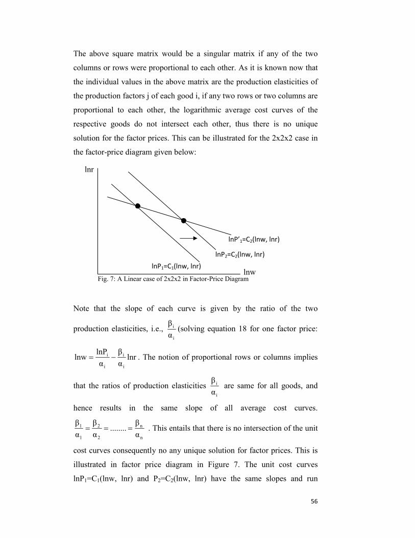
The above square matrix would be a singular matrix if any of the two

columns or rows were proportional to each other. As it is known now that

the individual values in the above matrix are the production elasticities of

the production factors j of each good i, if any two rows or two columns are

proportional to each other, the logarithmic average cost curves of the

respective goods do not intersect each other, thus there is no unique

solution for the factor prices. This can be illustrated for the 2x2x2 case in

the factor-price diagram given below:

No

pr

ln

th

he

αβ

co

ill

ln

lnr

Fig. 7: A Linear case of 2x2x2 in Factor-Price

te that the slope of each curve is give

oduction elasticities, i.e., i

i

αβ

(solving equat

lnrαβ

αlnP

wi

i

i

i −= . The notion of proportion

at the ratios of production elasticities i

i

αβ

nce results in the same slope of

n

n

2

2

1

1

αβ

........αβ

=== . This entails that there

st curves consequently no any unique solut

ustrated in factor price diagram in Figur

P1=C1(lnw, lnr) and P2=C2(lnw, lnr) have

lnP’1=C2(lnw, lnr)

lnP2=C2(lnw, lnr)

lnP1=C1(lnw, lnr)

Diagr

n by

ion

al ro

are s

all

is no

ion f

e 7.

the

lnw

56

am

the ratio of the two

18 for one factor price:

ws or columns implies

ame for all goods, and

average cost curves.

intersection of the unit

or factor prices. This is

The unit cost curves

same slopes and run

57

parallel without intersecting. In this case the matrix P in equation (30)

cannot be inverted and cannot have a unique solution for w.

All over again, this occurs if factor intensity reversal exists. Paul A.

Samuelson (1953) shows that this would be the case if the components θji

for just two factors are proportional in two industries even if the other

factor components are not. To solve for the changes in price in an N x N

setting, we can adjust the equations (22) and (23) from a 2x2 setting as

follows:

^

NNN

^

2N2

^

1N1

^

N

^

N1N

^

212

^

111

^

1

wθ..........wθwθP

............

wθ..........wθwθP

++=

++=

Since each price change equals the weighted factor price changes

0andθθ.......θθ 1N1N1211 >+++ , an increase in one commodity price Pi,

holding the others constant must be followed by an increase in at least one

factor price wj and a decrease in another factor price r. The increase in wj

is bigger than the increase in the commodity price so that,^^

i

^

j r0Pw >>> .

Consequently, the S-S theorem (2x2x2 model) can be generalized in the

sense that a commodity price change will result in a real gain to the

abundant factor and a loss to the other factor.

Summarizing the whole discussion, it can be maintained here that factor

prices are uniquely determined for commodity prices in cases of equal

number of goods and factors or even when goods are more than the

factors, given the equation 19 is invertible (i.e., no factor reversal

intensity). This is the case when the vector of factor prices is fully

determined by the vector of commodity prices and a given commodity

price change directly infers a definite factor price change. The goods’ and

factor prices’ association is the core foundation of the empirical estimation

58

of the factor price changes due to the goods’ price change. However, S-S

Theorem does not respond to the case when factors are more than the

goods. In price elasticity terms, we can illustrate the relationship between

wages and domestic prices in following way: i

j

lnP

lnw

∂

∂

Here wj is the price of factor j and Pi is the price of good i.

4.2 Trade Liberalization, Household Demand, and Welfare Effects

This part of the Chapter will open discussion on the impact of trade

liberalization on household demand and welfare using Marshallian and

Hicksian Approaches.

4.2.1 Household Expenditure

The changes in domestic prices of traded and nontraded goods as discussed

in sections 4.1.1 and 4.1.2 owing to the changes in the trade policy affect

the households’ demands. Adjustment in households’ demands also

changes the household utility level. The aim here is to seek the minimum

level of expenditure that maintains the households’ initial utility level

when domestic prices change. To better understand the concept of

expenditure function in its entirety, consider Figure 8:

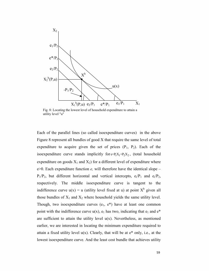
X

X

Ea

Fig

ex

iso

ex

e>

P1

res

ind

tho

Th

po

are

ea

att

low

Fig. 8: Locating the lowest level of household expenditure to attain a utility level "u"

ch of the pa

ure 8 repres

penditure to

expenditure

penditure on

0. Each expe

/P2, but dif

pectively.

ifference cu

se bundles

ough, two i

int with the

sufficient t

rlier, we are

ain a fixed u

est isoexpe

-P1/P2

rallel lines (so called isoexpe

ent all bundles of good X that

acquire given the set of

curve stands implicitly for

goods X1 and X2) for a differ

nditure function e, will there

ferent horizontal and vertica

The middle isoexpenditure

rve u(x) = u (utility level fix

of X1 and X2 where househol

soexpenditure curves (e1, e*

indifference curve u(x), e1 has

o attain the utility level u(x

interested in locating the min

tility level u(x). Clearly, that

nditure curve. And the least c

u(x)

e1/P2

e*/P2

e2/P2

2h(P,u)

Xh

nd

req

pric

1e=P

ent

fore

l i

c

ed

d yi

) h

tw

). N

imu

wi

ost

e1/P1

e*/P1 e2/P1 1h(P,u)

X2

iture curve

uire the sa

es (P1, P

1 2 2X +P X , (

level of ex

have the

ntercepts,

urve is

at u) at po

elds the sa

ave at lea

o, indicatin

evertheles

m expend

ll be at e*

bundle tha

X1

59

s) in the above

me level of total

2). Each of the

total household

penditure where

identical slope –

ei/P1 and ei/P2,

tangent to the

int Xh given all

me utility level.

st one common

g that e1 and e*

s, as mentioned

iture required to

only, i.e., at the

t achieves utility

60

u(x) at prices P1 and P2 will be the bundle h h1X =X (P,u)and h h

2X =X (P,u) . Here h

stands for “Hicksian”. If we denote the minimum expenditure necessary to

achieve required utility u(x) at prices Pi (representing set of prices P1 and

P2) by e (P, u), that level of expenditure will simply be equal to the cost of

bundle xh or h h1 1 2 2e(P,u)=P X (P,u)+P X (P,u)=e*. In more general terms,

expenditure function is expressed in following way [Mas-Colell, A. et al.

(1995)]:

n

+xÎRminp.xe(p,u)º subject to the constraint u(x) u≥ (31)

for all P values much greater than zero and all attainable utility levels u.

Note that any solution vector for this minimization problem would be

nonnegative and will depend on the parameters P and u. Also notice that if

u(x) is continuous28 and quasiconcave29, the solution will be unique, and

therefore we can denote the solution as the function hX (P ,u ) 0≥ . If this

solves the optimization problem, then the lowest expenditure necessary to

achieve utility u(x) at prices P1 and P2 will be exactly equal to the cost of

bundle h hX (P,u) or: e*P,u)=P.X (P,u) .

The above solution to the expenditure minimization problem is precisely

the consumer (household) vector of Hicksian or compensated demand

function. In fact, it is known that at a certain level of income, a change in

its given set of prices of goods will ordinarily lead to a subsequent change

in the household purchases and some corresponding change in initial level

of utility. Fixing the utility level at the initial point would help in

understanding how much an average household gains or loses from a price

change. To construct a hypothetical demand function, the whole process

must be observed by which when domestic prices fall a utility gain is

conferred on the household; it is compensated by reducing the household

28 No preference reversals 29 Balanced combination of quantities of both goods

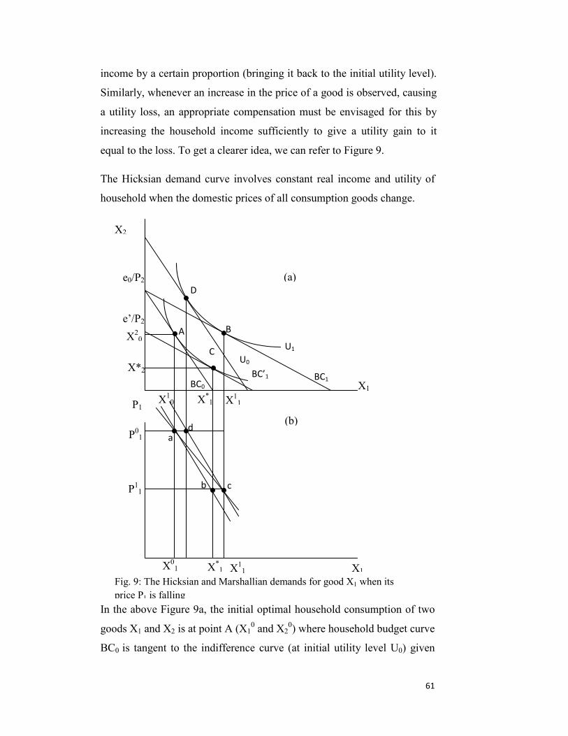
0 2

1

income by a certain proportion (bringing it back to the initial utility level).

Similarly, whenever an increase in the price of a good is observed, causing

a utility loss, an appropriate compensation must be envisaged for this by

increasing the household income sufficiently to give a utility gain to it

equal to the loss. To get a clearer idea, we can refer to Figure 9.

The Hicksian demand curve involves constant real income and utility of

household when the domestic prices of all consumption goods change.

In the above Figur

goods X1 and X2 is

BC0 is tangent to

D

d

X10

e 9a, the

at point

the indiff

X11

C

1 X1 Fig. 9: The Hicksian and Marshallian demands for good X1 when its price P is falling

initial optim

A (X10 and X

erence curv

(b)

(a)

al household co

20) where house

e (at initial utili

P1

X01

X*

c

b

a

P11

P01

e /P

e’/P2

X20

X*2

0

X*1

X1

1

X2

X1

A

B

U0

U1

BC1

BC’1 BC

61

nsumption of two

hold budget curve

ty level U0) given

62

the prices of two goods (P1 and P2) and expenditure e0. Allowing the fall in

the price of X1 from (P10) to (P1

1), while holding the price of X2 constant,

would tilt the budget curve outward on the horizontal axis, releasing more

income for the cheaper good X1. Thus the new budget curve BC1 is now

tangent to the higher indifference curve (U1) at point B, allowing the

household to consume more of good X1. The notion of HCV reflects how

much a household is willing to pay to remain at the initial utility level

(U0). This would imply that the household should move to point C (at

initial indifference curve and not necessarily at the same consumption

bundle), which would further mean that the household is obliged to give

up the amount increased in the real expenditure in terms of good X2. This

is reflected in the downward shift of the budget curve BC1 to BC’1 and

intercepts from e*/P2 to e’/ P2 on vertical axis. Now, owing to the altered

relative prices, the households adjust their consumption to the new optimal

bundle at C (X1* and X2*).

In contrast, the idea of Equivalent Variation (EV) is how much a

household is willing to receive to reach the new indifference curve (U1)

without the change in the price of any good (compare the points B and D

in Figure 9a.) It is measured by the difference of the expenditures on the

new indifference curve (U1) in points B and D.

In Figure 9b, Marshallian (uncompensated) and Hicksian (compensated)

demand curves are driven from the indifference map in Figure 9a. Curve

(ab) is the Hicksian (compensated) demand curve and (ac) is the

Marshallian (uncompensated) demand curve in Figure 9b. The Hicksian

(compensated) demand curve shows a smaller rise in the demand for X1

because the household is obliged to pay the compensating variation to stay

at the same utility level. The demand curve depicting the Equivalent

Variation is dc in Figure 9b referring to the indifference curve (U1) in

Figure 9a. Here for a price change, the HCV is the households’

willingness to pay and Equivalent Variation is the Households’

63

willingness to receive. HCV in Figure 9b can be seen as the area under the

compensated demand curve (ab) at initial utility (U0) which is P10abP1

1.

Likewise Equivalent Variation is represented by the area under

compensated demand curve dc at new indifference curve (U1) which is

P10dcP1

1. Similarly MCS can be seen as the area under the uncompensated

demand (ac), which is P10caP1

1. Marshallian and Hicksian welfare

measures are discussed in detail in 4.2.2 and 4.2.3.

The whole construction in Figure 9b represents Hicksian and Marshallian

demand curves for good X1. Briefly, the expenditure minimization

problem is just the vector of Hicksian demands because each of the

hypothetical “budget constraints” or isoexpenditure lines the household

faces in Figure 9a involves a level of expenditure exactly equal to the

minimum level necessary at the given prices to reach the original utility

level.

Thus, mathematical expression (31) contains important information on

Hicksian demands. Repeating the definition one more time, Hicksian

demand function, also known as compensated demand, is the demand of a

consumer over a bundle of goods that minimizes their expenditure while

delivering a fixed level of utility. 30

4.2.2 Change in Marshallian Consumers’ Surplus

Furthermore, as we identified that Hicksian demand curves are not readily

observable; we would relate Hicks’ idea of Compensating Variation to the

notion of Consumer Surplus, since the later is easily measured directly

from Marshallian demand. Consumer Surplus is the amount that

consumers benefit by being able to purchase a product for a price that is 30 The discussion on the utility maximization and expenditure minimization is inspired from Mas-Colell, A. et al. (1995).

64

less than they would be willing to pay at maximum. Here it is assumed

that the Cobb-Douglas utility function describes the households’

preferences.

∫=−=0

1

P

P

00001 )dPYq(P,)Y,CS(P)Y,CS(P∆CS

(32)

or

∑∑==

−=n

1i

1i

n

1i

2i CSCS∆CS (33)

CS∆ is the change in Consumer Surplus of a household, i is the number of

goods, ∑=

n

1i

1iCS is the Consumer Surplus with actual import tariff, and

∑=

n

1i

2iCS is the Consumer Surplus with the falling general tariff in the whole

economy.

The graphical representation of MCS can be followed in the Figure 9b

presented above. The mathematical calculation of the MCS is nothing but

the measurement of the area under the uncompensated demand curve

(P01P1

1ca in Figure 9b). This can be calculated in two parts. In the first

part, the change in the estimated Marshallian demand is calculated by

multiplying the estimated Marshallian demand (Xi) with the trade reforms

induced drop in the estimated domestic prices (P01- P1

1) of selected traded

and nontraded goods. Secondly, change in the estimated Marshallian

demand (X11-X0

1) is multiplied by the trade reform induced drop in the

estimated domestic prices (P01- P1

1) of the selected goods and divided by

two, because the area under the demand curve is being measured. The

summation of the two effects i.e. 2

)X)(XP(P)P(PX

01

11

11

011

10

1i

−−+− would

lead to the measurement of the area (P01P1

1ca) or MCS with selective

protection and with liberalizing trend in general economy. This estimate is

65

then divided by the average number of households to calculate the

households’ Marshallian Consumer Surplus.

4.2.3 Change in Hicksian Compensating Variation

To measure the impact of a tariff change on household welfare, the HCV

(willingness to pay) is measured from the estimated Hicksian Demand

Equations [Varian, H. R. (2003)]. The Hicksian Demand Equations are

estimated by isolating the substitution effect from the income effect of a

price change after solving the slutsky equation in the following way:

YX

XP

XPX i

ii

Ci

i

i

∂∂

+∂∂

=∂∂

(34)

i

Ci

PX∂∂

is the substitution effect of the price change, and YX

X ii ∂∂

is the

income effect of the price change. Equation (34) can be rewritten for the

pure compensated substitution effect, i.e., the household reaction toward a

price change at the unchanged utility, in the following way:

YX

XPX

PX i

ii

i

i

Ci

∂∂

−∂∂

=∂∂

(35)

The above expression can be used to evaluate the price change in natural

log terms by first converting it into elasticity approach:

YX

YY

XXP

XP

PX

XP

PX i

ii

i

i

i

i

iCi

i

i

Ci

∂∂

−∂∂

=∂∂

or

∂∂

−∂∂

=∂∂

YX

XY

YXP

XP

PX

XP

PX i

i

ii

i

i

i

iCi

i

i

Ci (36)

66

The term on the left hand side in equation (36) is the Hicksian Price

Elasticity of Demand. The first term on the right hand side is Marshallian

Price Elasticity estimated from the Marshallian demand curves, and the

second term has two parts. First one

YXP ii is the Budget Share of each

good, and the other one

∂∂

YX

XY i

i

is the income elasticity. Thus the

equation can further be revised in following way:

−= YηXYXP

PηXPηX iii

iMii

Ci

(37)

iCi PηX is the Hicksian Price Elasticity, i

Mi PηX is the Marshallian Price

Elasticity, and YηXi is the income elasticity of demand for all goods.

Hicksian Demand Equations for selected traded and nontraded goods can

then be calculated by replacing the parameters (coefficients) in

Marshallian Demand Equations by parameters estimated here (known as

Hicksian parameters) without including the income parameter since

Hicksian demand is not a function of income but utility. Since the both

demand curves (Marshallian and Hicksian) shift in parallel by similar

amounts from their old demand curves when the prices of other goods

change, the cross price elasticities in MCS and HCV remain same since

the effect of a change in the domestic price of one good on the demand for

the other good remains same in both cases. Further, the Household

Compensating Variation can be estimated from the information on the

Hicksian household expenditures. The exercise can be performed for

actual escalating tariff and for the falling general tariff rate.

Mathematically HCV is calculated on the same lines as the MCS is

calculated in the previous section, this time Marshallian demand estimates

are replaced by the Hicksian demand estimates.

67

4.2.4 Change in the Households’ Labour Income

As per Stolper-Samuelson (S-S) theory, the free trade benefits labour-

oriented sector and harms capital oriented sectors in a developing country

setting. By the virtue of S-S theory, the workers in agriculture (labour

oriented) should gain and the workers in manufacturing (capital oriented)

should lose when the trade is liberalized. Therefore the labour income in

agriculture and in manufacturing is estimated at the domestic prices at

actual escalating tariff and at the domestic prices if the tariff had followed

the falling trend in general economy. The difference in the estimated

labour income in both sectors will help identifying the gain and the loss of

workers in both sectors if the selected commodity groups had not been

protected.

The yearly agriculture and manufacturing labour incomes31 in log linear

form are estimated using backward regression method as per following

∑=

∂∂

+=n

1ii

i

iii0i L

LQ

Pαlnlnαlnw (38)

Here wi stands for the agriculture and manufacturing labour income. The

term on the right hand side in brackets

∂∂

ii

ii L

LQ

Pln is the labour

income earned by workers in the two sectors in the production of each

good (i.e. product of the calculated domestic prices of traded goods at

actual tariff Pi, marginal productivity of each good in both sectors

i

i

LQ∂∂

and the employed labour in each sector Li). The log linear equations

for estimation of marginal productivity in the two sectors are given here;

31 The labour incomes are reported in FBS books as monthly labour income, they are converted into yearly labour incomes by multiplying with 12.

68

∑=

+=n

1iii0i lnLααlnQ (39)

and

∑=

+=n

1iji0j lnLααlnQ (40)

Here Qi and Qj are the production variables and Li and Lj are the

employment variables in the production of each selected good in

agriculture and manufacturing respectively.

Theoretically, as mentioned in earlier paragraph, the agriculture labour

income is supposed to increase and the manufacturing labour income is

supposed to decrease. The difference between the two changes (increase in

agriculture and fall in manufacturing) would be the net gain or loss to the

households in general.

Thus the total effect of the trade reforms or protection is equal to the sum

total of the Hicksian change in household welfare and the change in the

labour income (LI).

∆LICV∆Yi += (41)

Here i∆Y is the change in total household income, CV is the

Compensating Variation for the household j and ∆LI is the change in the

household’s labour income.

69

4.2.5 Change in Poorest Households’ Welfare

The above model reflects only the change in the welfare of the average

household in Pakistan if the tariff on the selected commodity groups had

followed the trend in tariff in the whole economy. It does not reveal much

explicitly about how the poorest households are affected by the

protectionist policy. Also, as mentioned earlier, trade affects poverty via

direct and indirect transmission channels. These channels, as discussed in

Chapter 2, are economic growth and changes in domestic prices and labor

income. A relative change in domestic prices of consumable goods and the

wage tends to change the household consumption possibilities.32

The most relevant question of the study, thus, is how protectionist trade

policy is affecting the poorest households’ welfare. This is answered by

computing changes in the poorest household consumption patterns when

prices of traded and nontraded goods adjust due to the change in import

tariff. Information on the calculated domestic prices of traded and

nontraded goods with actual and falling general tariff (presented in 4.1.1

and 4.1.2) is combined with statistics on the percentage of poorest

households’ monthly income spent on each selected commodity. The

detailed Table on the percentage shares of poorest monthly households’

expenditure on selected household goods is provided in Appendix A1.1.

Data on the monthly poorest household expenditure (in percent) on all

traded and nontraded goods is available in Household Income Expenditure

Surveys of various years by the Statistical Division of Pakistan. Thus the

poorest households’ demand equation is given as:

)Y,P,f(PQ PoorestNTTPoorestd = (42)

32 See Winters (2000) for a discussion on the links between international trade and poverty.

70

or

)YδPδPδδQ Poorest3NT2T10Poorestd +++= (43)

It is assumed here that the values of iδ are same for all Pakistani

households irrespective of the income level. This is justified under the

Cobb-Douglas utility setting of the Pakistani households. Here Qdpoorest

represents the quantity of a good that a poorest household demands. This

is a function of the prices of traded goods PT, the prices of nontraded

goods PNT and the monthly income of the poorest households YPoorest. 0δ is

the constant and 1δ , 2δ and 3δ are the parameters for PT, PNT and Ypoorest.

The product of the calculated domestic prices at actual and at falling

general tariff and the demand quantities of the poorest households reflect

the yearly poorest household expenditure on the selected goods in both

cases. Here it should be noted that the Cobb-Douglas utility function

depicts the poorest households’ preferences.

The yearly expenditure of the poorest household on each commodity in

money (PKR) terms is calculated by multiplying the percentage budget

share devoted for each household commodity with the poorest household

yearly income33. Further, the actual quantity of the selected goods

demanded by the poorest households is calculated from the ratio of the

yearly expenditure in PKR and the calculated domestic prices at actual and

at the general falling tariff.

The calculated poorest households’ demand equations are then used to

determine the MCS by measuring the gap between household expenditure

at actual escalating tariff and at falling tariff in general. It is done in the

similar way as the MCS for the average households estimated earlier:

33 Assumption of expenditure on any given good is a constant fraction of total household income. (Cobb-Douglas utility Function)

71

∑∑==

−≡n

1i

poorest1i

n

1i

poorest2i

poorest1 CSCS∆CS (44)

Here CSPoorest stands for the Consumer Surplus for the poorest households;

∑=

n

1i

poorest1iCS is the initial MCS for the poorest households at actual tariff and

∑=

n

1i

poorest2iCS is the MCS for the poorest households when the tariff is

following the general falling trend.

The mathematical calculation of MCS for poorest households is performed

in the similar way as for MCS for ordinary households by inserting the

calculated poorest households’ demands instead of estimated Marshallian

demands for average households.

72

5 Statistical Results and Interpretation

As discussed in Chapter three, the General Equilibrium modeling

technique does not provide empirical validation of the long time series

dataset (36 years data on domestic prices, PCI and consumption for the

demand estimation and 14 years data for measurement of households’

welfare), hence the trade-poverty link is estimated using Partial

equilibrium approach while holding the General Equilibrium framework at

the root of the analysis. The approach is adapted so since the theoretical

background of the study is based on the Stolper-Samuelson model

(extended by including the nontraded goods) which is built on the General

Equilibrium approach.

The main sources of data are FBS’ book ‘50 years of Pakistan in

Statistics’ all volumes and FBS online statistics portal34; online datasets of

Federal Board of Revenue (FBR), Pakistan, a public sector organization

formerly known as Central Board of Revenue responsible for collecting all

types of tax revenues and framing national tariff policies35; Food and

Agriculture Organization (FAO) online datasets; Household Income and

Expenditure Surveys (FBS); Labour Force Surveys (FBS) and the

International Labour Organization (ILO) online dataset. Due to the

unavailability of straight forward data on domestic and international prices

and tariff rates, the appropriate data has been calculated from available

statistics before using in the study. The detailed description on the

calculation and quality of data used in the study is provided in the

following paragraphs.

34 http://statpak.gov.pk/depts/index.html 35 http://www.fbr.gov.pk/

73

5.1 Data

Following sections present the issues related to the quality and availability

of the data used on the domestic and international prices of all selected

goods, international trade, per capita income and the poorest household

expenditure on the selected goods. Before hand, the household food items

happen to be heterogeneous in nature therefore to avoid any ambiguity

regarding the names of the consumer goods selected for the study they are

briefly elaborated in the following Text Box. The names of the nonfood

items such as electricity, gas, firewood, cigarettes, and tea are self

explanatory, yet other food items need description with regard to their

names in the international datasets. The detailed table to identify the

selected goods at the data sources is given in Appendix A1.2.

5.1.1 Import Tariff and International and Domestic Prices

The data on the import tariff revenue from 1992 to 2005 is collected from

the Federal Board of Revenue (FBR) on various commodity groups.

Amongst, the selected commodity groups are fruits, nuts and vegetables;

Text Box: Description on domestic prices and production of selected traded and nontraded goods 1. Rice: Basmati (milled) rice 2. Milk: cow milk as cow and buffalo milk is on average more than 96% of

total milk production and total milk production. 3. Pulses: The average moong (green beans) split and washed and gram split

and the production of pulses nes (Not Elsewhere Specified). 4. Beef: Cattle and Buffalo meat 5. Mutton: Goat meat 6. Sugar: Refined Sugar 7. Vegetable Oil: Ghee, vegetable dalda tin 2.5 KGs converted into price per ton 8. Cigarettes: K2 cigarettes price per packet (converted from price per 1000

grams to price per ton and production in tons 9. Chicken meat: Chicken farm/poultry 10. Other vegetables: Vegetables fresh nes 11. Kerosene oil: Crude Oil 12. Spices: Spices nes (Not Elsewhere Specified)

74

tea, coffee and spices; milk butter and cheese; animal and vegetable oil;

edible cereals and vegetables; tobacco; fuels and oils; sugar and

confectionary; and meat, fish and other preparations. The tariff per ton on

each commodity group is calculated by dividing the total yearly tariff

revenue in PKR for 1992-2005 by the total import (C.I.F) quantity in tons

of all varieties of goods in the respective commodity group. For example,

the tariff per ton in PKR on the commodity group of meat, fish and other

preparations is calculated by dividing the total tariff revenue in PKR

collected from the commodity group by the total sum of the import

quantities in tons of all the varieties of meat (including meat, beef, chicken

meat and fish).36 As discussed in Chapter 1, the average calculated tariff

on the selected commodity groups is escalating37 in contrast to the falling

general tariff indicating a selective protectionist trade policy in the

country. The import tariff per ton on all commodities is recalculated in

line with the falling trend in the general tariff to calculate new domestic

prices to measure the loss in the households’ welfare due to selective trade

protectionist policy. The new commodity-wise tariff rates are calculated

by allowing the actual commodity-wise tariff to fall corresponding to the

general falling tariff with 1992 as the base year. The selection of the 1992

as the base year brings about zero difference between actual and the

general falling tariff and the domestic prices at both tariffs in the year

1992.

International prices are calculated by dividing the total import or export

value (in PKR) by the import or export quantities in tons for all selected

traded goods for the 1992-2005 period. There were some missing values

which are replaced by interpolation method. 36 Real world tariff rates (in percentage) are available from WTO online dataset for 1999-2002 and 2004-2005 on some goods (presented in A 4.5). These tariff rates on various goods are used as a benchmark to verify the reliability and accuracy of the average calculated tariff. The domestic prices calculated at the average calculated and real world tariff rates are nearly overlapping in some cases (pulses, milk vegetable oil, and tea) and in other cases they are better indicators of domestic prices than the estimated domestic prices at calculated tariff. See graph 10 and Appendix A1.3 37 For a discussion on import tariff on selected commodities see Chapter 1.

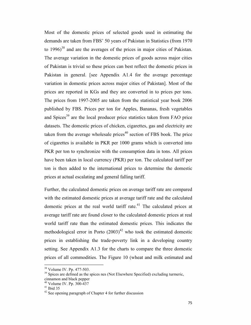
75

Most of the domestic prices of selected goods used in estimating the

demands are taken from FBS’ 50 years of Pakistan in Statistics (from 1970

to 1996)38 and are the averages of the prices in major cities of Pakistan.

The average variation in the domestic prices of goods across major cities

of Pakistan is trivial so these prices can best reflect the domestic prices in

Pakistan in general. [see Appendix A1.4 for the average percentage

variation in domestic prices across major cities of Pakistan]. Most of the

prices are reported in KGs and they are converted in to prices per tons.

The prices from 1997-2005 are taken from the statistical year book 2006

published by FBS. Prices per ton for Apples, Bananas, fresh vegetables

and Spices39 are the local producer price statistics taken from FAO price

datasets. The domestic prices of chicken, cigarettes, gas and electricity are

taken from the average wholesale prices40 section of FBS book. The price

of cigarettes is available in PKR per 1000 grams which is converted into

PKR per ton to synchronize with the consumption data in tons. All prices

have been taken in local currency (PKR) per ton. The calculated tariff per

ton is then added to the international prices to determine the domestic

prices at actual escalating and general falling tariff.

Further, the calculated domestic prices on average tariff rate are compared

with the estimated domestic prices at average tariff rate and the calculated

domestic prices at the real world tariff rate.41 The calculated prices at

average tariff rate are found closer to the calculated domestic prices at real

world tariff rate than the estimated domestic prices. This indicates the

methodological error in Porto (2003)42 who took the estimated domestic

prices in establishing the trade-poverty link in a developing country

setting. See Appendix A1.3 for the charts to compare the three domestic

prices of all commodities. The Figure 10 (wheat and milk estimated and 38 Volume IV. Pp. 477-503. 39 Spices are defined as the spices nes (Not Elsewhere Specified) excluding turmeric, cinnamon and black pepper 40 Volume IV. Pp. 300-437 41 Ibid 35 42 See opening paragraph of Chapter 4 for further discussion

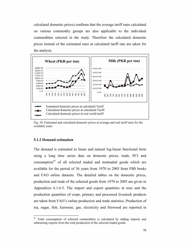
calculated domestic prices) confirms that the average tariff rates calculated

on various commodity groups are also applicable to the individual

commodities selected in the study. Therefore the calculated domestic

prices instead of the estimated ones at calculated tariff rate are taken for

the analysis.

Fig. 10: Estimated and calculated domestic prices at averaavailable years

5.1.2 Demand estimation

The demand is estimated in linear and natural

using a long time series data on domestic

consumption43 of all selected traded and no

available for the period of 36 years from 1970

and FAO online datasets. The detailed tables

production and trade of the selected goods from

Appendices 6.1-6.5. The import and export q

production quantities of crops, primary and pro

are taken from FAO’s online production and tra

tea, sugar, fish, kerosene, gas, electricity and

43 Total consumption of selected commodities is calcsubtracting exports from the total production of the selecte

Wheat (PKR per ton)

Estimated domestic prices at calculated Tariff Calculated domestic prices at calculated Tariff Calculated domestic prices at real world tariff

Milk (PKR per ton)

76

ge and real tariff rates for the

log-linear functional form

prices, trade, PCI and

ntraded goods which are

to 2005 from FBS books

on the domestic prices,

1970 to 2005 are given in

uantities in tons and the

cessed livestock products

de statistics. Production of

firewood are reported in

ulated by adding imports and d traded goods.

77

FBS’ 50 years of Pakistan in statistics44 and statistical year book 2007 of

Pakistan. Production of cigarettes is taken from the United States

Agriculture Department in million pieces.45 The data on household total

expenditure in PKR and commodity-wise expenditure as percentage of

total expenditure and per capita income are collected from FBS.

Household surveys in Pakistan are not conducted on a yearly basis. Owing

to intermittent regime changes, the tasks of household surveys have been

suffering from big time lags. Therefore some of the segments on the

required household data, like yearly time series data on average and the

poorest households’ expenditures on selected traded and nontraded goods

do not contain complete information for 36 years. Therefore the values

for the missing years have subsequently been generated by interpolation

method.

Further, owing to the unavailability of the required data series on the

consumption of the selected traded and nontraded goods by the poorest

households in Pakistan, the poorest household demand equations are not

estimated; rather they are calculated from the available information on the

poorest households’ budget shares allocated for consumption of the

selected traded and nontraded goods, the annual household income and the

actual and general import tariff embedded domestic prices. The average

budget shares allocated to the consumption of the selected traded and

nontraded goods and the poorest households’ income and PCI are

presented in Appendix A1.1. The complete data on working hours in the

selected employment (agriculture and manufacturing) sectors for the study

period are not available. However, the available data on yearly labour

44 Sugar and tea in Volume III. p. 348 and in statistical year book 2007 p 260.; fish in volume III, p. 319 and in statistical year book 2007 p. 69; kerosene, gas and electricity in volume III, p. 328 and in statistical year book 2007 p. 155-157; firewood in volume III, p. 317. 45 Production in million pieces is converted into tons by dividing the number by 2,000,000 as the study has taken the approximate weight for one cigarette equal to 2 grams.

78

income implicitly counts for both the working hours and the

corresponding wage rate.

5.1.3 Domestic Prices and Labour Income

The detailed classification of agriculture and manufacturing workers

allocated to the production of each good separately is not available from

the labour force surveys of Pakistan. Therefore the labour employment in

the production of each good in agriculture and manufacturing is

approximated from the production shares of each good in the two sectors.

For example, the wheat production is on average only 15.49% of total

agriculture production, it is assumed that the labour employed in the

production of wheat is 15.49% of the total agriculture labour. Similarly the

production of tea is on average 0.81% of total manufacturing production,

the labour employed in the production of tea is assumed to be 0.81% of

the total manufacturing labour. By this hypothetical assumption it is

assumed that the marginal labour productivity in the selected goods is

constant which may not be true, nevertheless instead of using the total

agriculture and manufacturing labour which produces highly exaggerated

results46 on labour income generated from the production of each selected

good, this assumption can fairly correct for the exaggeration. See section

5.4.1 for a more detailed discussion on the subject in question.

Beside all the weaknesses, since all the data is collected from government

organization/ministries and international organizations, it is taken to be

unambiguously reliable for the research study.

46 The total labour income in agriculture seems to be exaggerated by the multiplication factor of 13 (number of agriculture goods) and in manufacturing by 7 (number of manufactured goods).

79

5.1.4 Exclusion of Goods from the Model

Though, intuitively, it can be argued that the liberalized trade policy

potentially can affect the whole basket of household consumption goods.

Nonetheless, due to various reasons such as data availability,

heterogeneity of household items and percentage share of household

expenditure on the items in question, some items have been excluded from

the scope of the study. Broadly, the following criteria have been adapted

to exclude the items from the analysis:

1. Item is not included because the availability of data is an issue. For

example: Rent is a nontradable good and the issue of availability of

quality data on rent remains questionable. Further, most of the

poorest in Pakistan are found staying in rural areas where the

concept of renting a house or an apartment is not as established as

it is in urban centers. It is so because almost all of the economic or

social activities such as school teaching, retail business, cropping

or other live stock activities are performed by the local residents of

the village and all villagers own their houses. Only the individuals

from government bodies such as health or education department

stay in the rural areas as outsider and mostly they are provided the

residence facilities in the same buildings where they work or the

villagers collectively arrange their stay. Secondly, Household

expenditure on rent as recorded in household surveys shows that

80% of household expenditure on rent is not explicitly spent on it

rather it is implicit. That means the amount shown under the head

of rent is not actually spent but it is the expenditure that seems to

be “saved” by poorest Households due to the “owner occupied

houses”. Other items not included here on the basis of the similar

80

presuppositions are given as under: Health, Cleaning and Laundry,

education, entertainment and recreation and Transport.

2. Item is not included because the expenditure on it as a percentage

of the total expenditure is minimal and negligible, not able to

influence the total expenditure of a poorest household

significantly. These items are: Baked and fried products, dry and

condensed milk, mustard oil, salt, eggs, coffee and other soft

drinks.

3. Item is not included because it is classified incompletely or

unclearly and is heterogeneous in nature and the collection of

individual data is too cumbersome or the good has been specified

in a very broad sense. These items are: Other cereals, other milk

products, other sugar products, ready-made food products and

other tobacco products.

On average the selection of the goods allows the present study to cover

50.77% of the total monthly household expenditure of the poorest

households (Appendix A1.1)

5.2 Regression Analysis

The statistics used in the present study originate from the national time

series data from Pakistan and no sample data is used. Therefore the

regression analysis here is performed as the descriptive statistics which

aims to summarize a data set quantitatively and portrays the relationships

among variables as they are without employing a probabilistic

formulation. In case of using sample data for regression analysis, the

researcher is confronted to inter alia two big issues which can put a

question on the reliability of the whole exercise and the results. These are:

correlation of the error terms or serial autocorrelation and different

81

variances or the heteroscedasticity. The use of heteroscedastic data does

not produce biased OLS coefficient estimates; instead it may produce

biased OLS estimates of the variance and the standard errors of the

coefficients. On the other hand, leaving unbiased OLS estimates, the serial

autocorrelation causes overestimation in the true variance of Beta,

underestimation of the estimated Beta, inflated t-stats and R2. This may

produce results looking more accurate than they actually are. Further, the

significant t-values are the indicators of the power of results estimated

from one sample to be generalized over other samples of the population.

Since, no sample data are used in the present study hence the issues arising

from the possible correlation of the error terms or different variances and

t-test significance are out of the scope. Only the large R2 values suffice the

reliability and efficiency of the regression results.47

After detailed description on the issues related to data, regression issues

and the selection of the goods in the above paragraphs, the rest of the

Chapter is divided in two parts. In the first part, the determination of the

domestic prices of traded goods at actual tariff and the falling tariff in

general is discussed. The discussion is further extended to the estimated

link of the domestic prices of traded goods with the domestic prices of

nontraded goods at actual and the falling tariff in general. Then follows the

interpretation of the impact of the trade liberalization/selective protection

on the household demand and consumption patterns for all traded and

nontraded goods via household demand equations. In the second part, the

estimation of the resulting change in the average household welfare (MCS

and HCV) is interpreted. Subsequently, the empirical results on the change

in the welfare of the poorest households in Pakistan when the tariff

follows the falling trend in the general economy are interpreted and

explicated. Finally, the estimated links between domestic prices and the

labour income in agriculture and manufacturing are interpreted. The

47 Gujarati, D. N. (2004)

82

Chapter is concluded with separate sections devoted to discussion of the

results and the limitations of the estimated interrelations.

5.3 Change in the Domestic Prices of Traded and Nontraded Goods

and Households’ Demand

The discussion on the calculated domestic prices of traded and estimated

domestic prices of nontraded goods at actual tariff and the case when the

tariff rate follows the general tariff is presented in the following section.

5.3.1 Change in the Domestic Prices of Traded Goods

The link between domestic prices and the import tariff rate given

international prices is established as per the given price-tariff

relationship P =P +ti wi i . The domestic price (Pi) of a traded good is

determined by the import tariff per ton (ti) levied on the traded good plus

the international price of the good (Pwi). Since both the determinants of the

domestic prices (import tariff originating from the trade policy of a

country and international prices determined by world demand and

supply48) are exogenous variables therefore the domestic prices of all

traded goods are calculated by inserting the values of yearly import tariff

and the international prices for the period of 1992 to 2005 in the above

price-tariff relationship. The 14-year averages of the calculated domestic

prices at actual escalating and at the falling general tariff rates given the

international prices are presented in the following Table 1. The domestic

prices calculated at actual and at falling general tariff (in PKR per ton) for

all selected traded and nontraded goods for all years are provided in

48 Pakistan being a small open economy is a price taker.

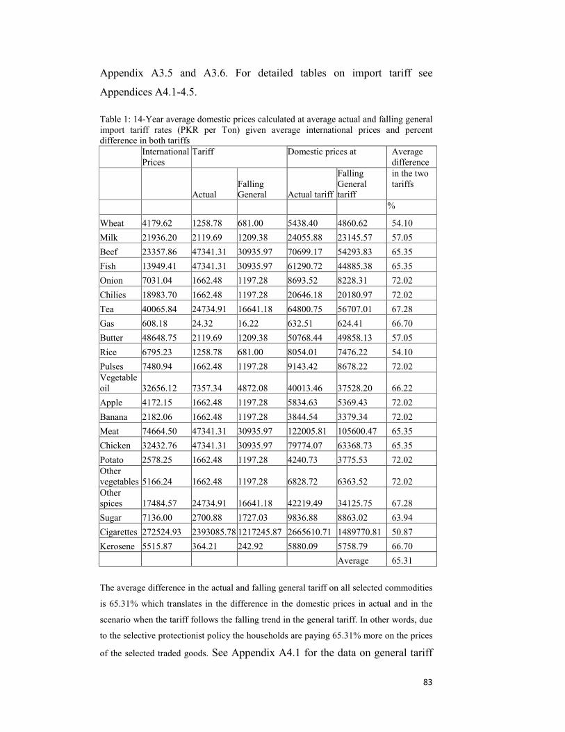
83

Appendix A3.5 and A3.6. For detailed tables on import tariff see

Appendices A4.1-4.5.

Table 1: 14-Year average domestic prices calculated at average actual and falling general import tariff rates (PKR per Ton) given average international prices and percent difference in both tariffs International

Prices Tariff Domestic prices at Average

difference

Actual Falling General Actual tariff

Falling General tariff

in the two tariffs

%

Wheat 4179.62 1258.78 681.00 5438.40 4860.62 54.10

Milk 21936.20 2119.69 1209.38 24055.88 23145.57 57.05

Beef 23357.86 47341.31 30935.97 70699.17 54293.83 65.35

Fish 13949.41 47341.31 30935.97 61290.72 44885.38 65.35

Onion 7031.04 1662.48 1197.28 8693.52 8228.31 72.02

Chilies 18983.70 1662.48 1197.28 20646.18 20180.97 72.02

Tea 40065.84 24734.91 16641.18 64800.75 56707.01 67.28

Gas 608.18 24.32 16.22 632.51 624.41 66.70

Butter 48648.75 2119.69 1209.38 50768.44 49858.13 57.05

Rice 6795.23 1258.78 681.00 8054.01 7476.22 54.10

Pulses 7480.94 1662.48 1197.28 9143.42 8678.22 72.02 Vegetable oil 32656.12 7357.34 4872.08 40013.46 37528.20 66.22

Apple 4172.15 1662.48 1197.28 5834.63 5369.43 72.02

Banana 2182.06 1662.48 1197.28 3844.54 3379.34 72.02

Meat 74664.50 47341.31 30935.97 122005.81 105600.47 65.35

Chicken 32432.76 47341.31 30935.97 79774.07 63368.73 65.35

Potato 2578.25 1662.48 1197.28 4240.73 3775.53 72.02 Other vegetables 5166.24 1662.48 1197.28 6828.72 6363.52 72.02 Other spices 17484.57 24734.91 16641.18 42219.49 34125.75 67.28

Sugar 7136.00 2700.88 1727.03 9836.88 8863.02 63.94

Cigarettes 272524.93 2393085.78 1217245.87 2665610.71 1489770.81 50.87

Kerosene 5515.87 364.21 242.92 5880.09 5758.79 66.70

Average 65.31

The average difference in the actual and falling general tariff on all selected commodities

is 65.31% which translates in the difference in the domestic prices in actual and in the

scenario when the tariff follows the falling trend in the general tariff. In other words, due

to the selective protectionist policy the households are paying 65.31% more on the prices

of the selected traded goods. See Appendix A4.1 for the data on general tariff

84

in the economy and Appendices A4.2 A4.3 and A4.4 for the calculation of

actual and the falling commodity-wise import tariff from import revenue

in PKR and import quantities in tons.

5.3.2 Change in the Domestic Prices of Nontraded Goods

The empirical link between domestic prices of traded and nontraded goods

in the S-S setting has been established in natural log linear form using

stepwise backward regression method in T

NTTNT lnP

lnPdlnPdlnP

∂∂

= setting. Here

lnPNT and lnPT are the natural log domestic prices of nontraded and traded

goods, respectively. The impact of a change in the calculated prices of

traded goods on the domestic prices of two nontraded goods is estimated

for firewood and electricity individually. The estimations in the case of

electricity confirm that the calculated domestic prices of 12 out of 22

traded goods influence the price of electricity (nontraded good). These

goods are rice, pulses, bananas, apples, potatoes, other vegetables, chilies,

spices, gas, beef, chicken, and tea. The average predicted impact on the

domestic price of electricity is negative. The same is repeated for firewood

and found that the calculated domestic prices of 13 out of 22 traded goods

influence its domestic price. These goods are: wheat, rice, milk, vegetable

oil, apples, mutton, potatoes, other vegetables, chilies, sugar, gas, tea, and

butter and ghee. The average predicted impact on the domestic price of

firewood is positive. The summary of the empirical results is provided in

Tables 2 and 3 for both nontraded goods.

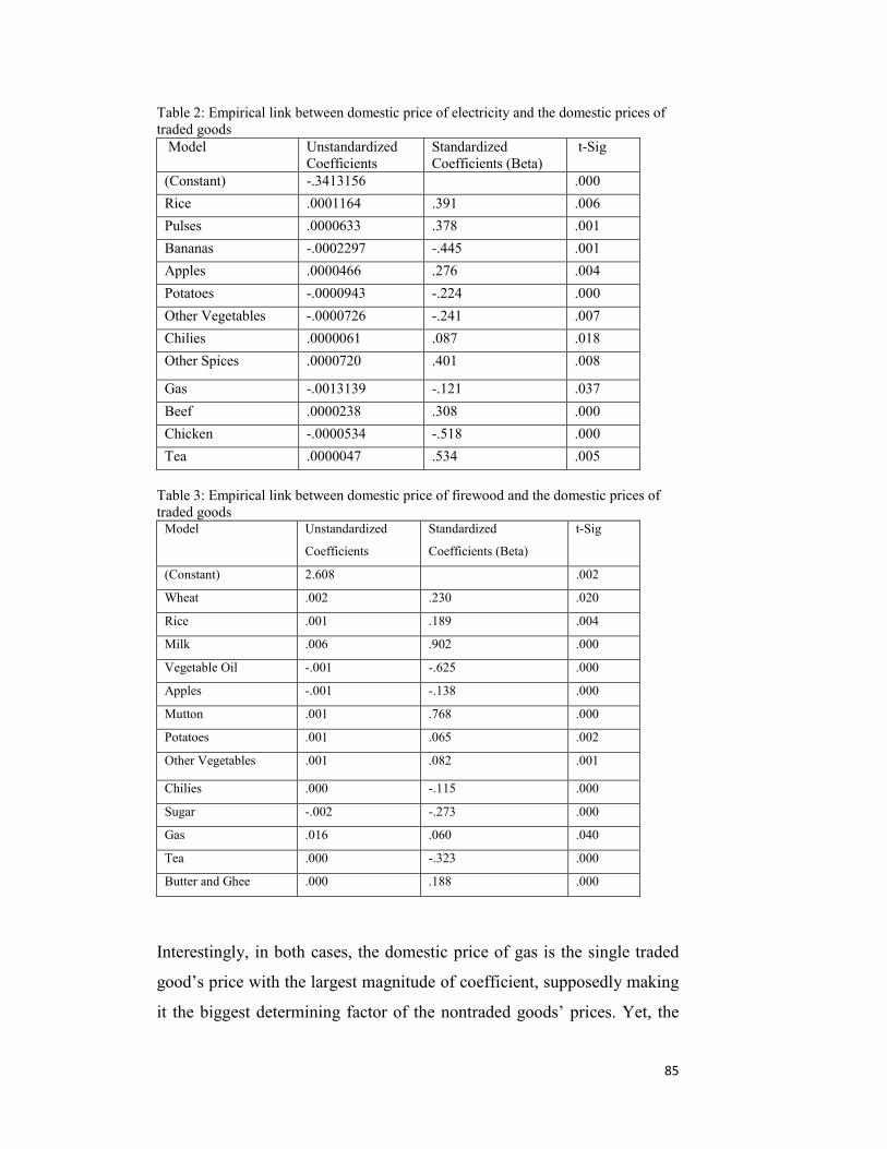
85

Table 2: Empirical link between domestic price of electricity and the domestic prices of traded goods

Model Unstandardized Coefficients

Standardized Coefficients (Beta)

t-Sig

(Constant) -.3413156 .000

Rice .0001164 .391 .006

Pulses .0000633 .378 .001

Bananas -.0002297 -.445 .001

Apples .0000466 .276 .004

Potatoes -.0000943 -.224 .000

Other Vegetables -.0000726 -.241 .007

Chilies .0000061 .087 .018

Other Spices .0000720 .401 .008

Gas -.0013139 -.121 .037

Beef .0000238 .308 .000

Chicken -.0000534 -.518 .000

Tea .0000047 .534 .005

Table 3: Empirical link between domestic price of firewood and the domestic prices of traded goods

Model Unstandardized

Coefficients

Standardized

Coefficients (Beta)

t-Sig

(Constant) 2.608 .002

Wheat .002 .230 .020

Rice .001 .189 .004

Milk .006 .902 .000

Vegetable Oil -.001 -.625 .000

Apples -.001 -.138 .000

Mutton .001 .768 .000

Potatoes .001 .065 .002

Other Vegetables .001 .082 .001

Chilies .000 -.115 .000

Sugar -.002 -.273 .000

Gas .016 .060 .040

Tea .000 -.323 .000

Butter and Ghee .000 .188 .000

Interestingly, in both cases, the domestic price of gas is the single traded

good’s price with the largest magnitude of coefficient, supposedly making

it the biggest determining factor of the nontraded goods’ prices. Yet, the

86

Beta Standardized Coefficients in both cases present a contradictory

picture. The Beta Standardized Coefficient for the price of gas assumes the

lowest value -0.121 in case of electricity and 0.60 in case of firewood. Due

to the high comparability power of the beta coefficients, it is explicitly

inducted that, despite the large magnitude of the non-standardized

coefficient of the gas price, the important determinants of the electricity

price are the domestic prices of tea, chicken, bananas, and other spices

with the higher Beta Standardized coefficients’ Values (0.534, 0.518,

0.445, and 0.401, respectively). In the case of firewood, the domestic

prices of milk, mutton, and vegetable oil are the most important

determinants with the highest Beta Standardized Coefficients’ values

(0.902, 0.768, and -0.625, respectively). Despite the large magnitude of

the non-standardized coefficients, in standardized coefficients the gas

price in the case of both goods is the least important determinant of the

domestic prices of electricity and firewood.

The positive influence of the gas price on the price of firewood is indeed a

convincing result as gas and firewood are closely related to each other in

the energy sector, since the firewood is used as a close substitute for the

gas.

As mentioned earlier, the estimated reaction of the domestic price of one

nontraded good (i.e., electricity) has been negative to the tariff-induced

fall in the domestic prices of some traded goods. This means that as the

domestic prices of the selected traded goods are falling, the domestic price

of electricity is rising. This can be explained in the following way.

Electricity is a major source of generation of power demanded in the

manufacturing and agriculture production of the country. It is used as the

key input factor in the production of selected (and all) traded goods. Fall

in the domestic prices of traded goods at falling general tariff provides the

households an opportunity to demand more of the household goods. In

response to the rise in the household demand for the consumer goods, the

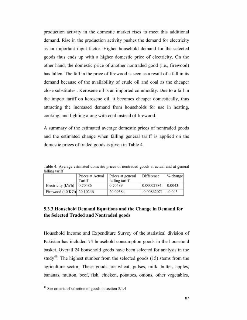
87

production activity in the domestic market rises to meet this additional

demand. Rise in the production activity pushes the demand for electricity

as an important input factor. Higher household demand for the selected

goods thus ends up with a higher domestic price of electricity. On the

other hand, the domestic price of another nontraded good (i.e., firewood)

has fallen. The fall in the price of firewood is seen as a result of a fall in its

demand because of the availability of crude oil and coal as the cheaper

close substitutes.. Kerosene oil is an imported commodity. Due to a fall in

the import tariff on kerosene oil, it becomes cheaper domestically, thus

attracting the increased demand from households for use in heating,

cooking, and lighting along with coal instead of firewood.

A summary of the estimated average domestic prices of nontraded goods

and the estimated change when falling general tariff is applied on the

domestic prices of traded goods is given in Table 4.

Table 4: Average estimated domestic prices of nontraded goods at actual and at general falling tariff

Prices at Actual Tariff

Prices at general falling tariff

Difference % change

Electricity (kWh) 0.70486 0.70489 0.00002784 0.0043

Firewood (40 KG) 20.10246 20.09384 -0.00862071 -0.043

5.3.3 Household Demand Equations and the Change in Demand for the Selected Traded and Nontraded goods

Household Income and Expenditure Survey of the statistical division of

Pakistan has included 74 household consumption goods in the household

basket. Overall 24 household goods have been selected for analysis in the

study49. The highest number from the selected goods (15) stems from the

agriculture sector. These goods are wheat, pulses, milk, butter, apples,

bananas, mutton, beef, fish, chicken, potatoes, onions, other vegetables,

49 See criteria of selection of goods in section 5.1.4

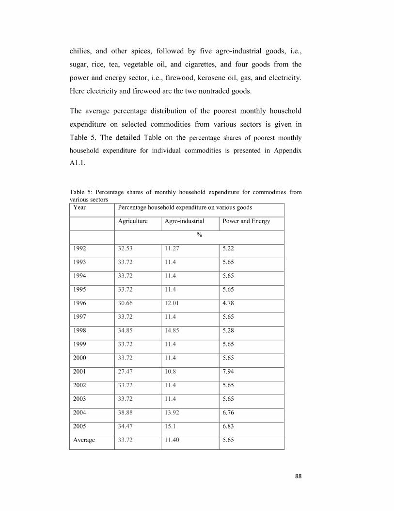
88

chilies, and other spices, followed by five agro-industrial goods, i.e.,

sugar, rice, tea, vegetable oil, and cigarettes, and four goods from the

power and energy sector, i.e., firewood, kerosene oil, gas, and electricity.

Here electricity and firewood are the two nontraded goods.

The average percentage distribution of the poorest monthly household

expenditure on selected commodities from various sectors is given in

Table 5. The detailed Table on the percentage shares of poorest monthly

household expenditure for individual commodities is presented in Appendix

A1.1.

Table 5: Percentage shares of monthly household expenditure for commodities from various sectors

Year Percentage household expenditure on various goods

Agriculture Agro-industrial Power and Energy

%

1992 32.53 11.27 5.22

1993 33.72 11.4 5.65

1994 33.72 11.4 5.65

1995 33.72 11.4 5.65

1996 30.66 12.01 4.78

1997 33.72 11.4 5.65

1998 34.85 14.85 5.28

1999 33.72 11.4 5.65

2000 33.72 11.4 5.65

2001 27.47 10.8 7.94

2002 33.72 11.4 5.65

2003 33.72 11.4 5.65

2004 38.88 13.92 6.76

2005 34.47 15.1 6.83

Average 33.72 11.40 5.65

89

It is known from Table 5 that the biggest portion of the average household

expenditure on selected goods (33.72%) is devoted to goods coming from

agriculture followed by goods from the agro-industrial sector (11.4%) and

power and energy (5.65%). Similarly the highest number of goods

consumed by the households in the country is produced in agriculture

(fifteen goods) followed by agro-industrial (five goods) and power and

energy (four goods).

The demand equations estimated for the selected goods depict the

consumption patterns vis-à-vis the domestic prices of the consumption

goods. The change in domestic prices of the goods alters the amount of the

good the households prefer to consume. With a rise in the domestic price

of a good, households adjust their demand for that good downward,

usually by substituting it with the relatively cheaper goods. Similarly,

households buy more of a good when its price in the local market falls.

Therefore the households’ welfare and the consumption possibilities the

households face change with the adjustments in the domestic prices they

pay. Hence, it is essential to investigate how the household’s consumption

arrangements of diverse goods change as the domestic prices of the goods

they consume change. This can be known from the household demand

equations for all the goods they consume. In the following section the

estimated Marshallian demand is discussed in detail.

5.3.3.1 Estimated Marshallian Demand

Marshallian demand is estimated for selected goods using OLS regression

method in linear and log linear functional forms to obtain statistically significant

estimations with a maximal R2. The yearly data on actual domestic prices of

selected goods, their substitutes’ and complementary goods’ prices including

90

applied actual tariff rates and PCI50 for 1970 to 2005 period have been included

as the independent variables. The estimated Marshallian demand equations

for the selected household goods depict a normal (negative) Price-Demand

relationship, which is in line with the conventional demand theory Q =f(P ,P ,P ,PCI)i c s for 20 out of 24 goods. (Here Q stands for quantity

demanded, Pi are the own prices of the selected traded and nontraded

goods, Pc and Ps are the prices of other (complementary and substitute)

goods. All the models maintain overall reliability of the relationships and

estimates with large values of R-square and significant F-values. In view

of the fact that the household demand equations are derived from the

national data for Pakistan and no sample data has been used, the

requirement of p-value of t-statistics below 1% in case of all models has

been compromised (see 5.2 for a brief discussion). All estimated demand

equations are provided in Appendix A2.

In the case of four goods (sugar, chilies, beef, and fish), the coefficients of

the own prices assume a positive sign. It seems most probable that the

unconventional signs of the own price coefficients in case of these goods

are the result of certain other factors causing a shift in the demand for

these goods which are beyond the scope of this study.

On the other hand, demand for all goods but pulses are positively

associated with income, which is in conformation with an average

Pakistani household consumption pattern. Pulses show a negative

association with household income; it is treated as an inferior good since

households with additional income move away from demand for pulses to

close substitutes, resulting in a fall in the demand for pulses when

50 As data on Household Income is only available for intermittent years between 1970 and 2005 the missing values in the Household Income data series are generated by interpolation method in PASW 18. However PCI is available for 36 years from 1970 to 2005. Therefore PCI has been used in estimation of Household demands to obtain statistically significant results.

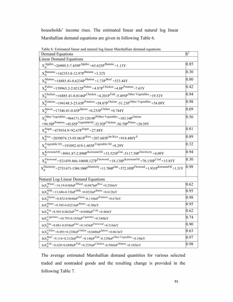
91

households’ income rises. The estimated linear and natural log linear

Marshallian demand equations are given in following Table 6.

Table 6: Estimated linear and natural log linear Marshallian demand equations Demand Equations R2

Linear Demand Equations Apples Apples BananadX =26909.5-7.459P +65.625P +1.13Y 0.85

Bananas BananadX =142353.8-12.97P +3.32Y 0.30

Mutton Mutton BeefdX =16885.41-0.6234P +1.73P +533.44Y 0.80

Pulses Pulses Chicken PotatoesdX =159965.2-2.0212P +4.97P +4.8P -7.63Y 0.42

Chicken Chicken Fish Other VegetablesdX =16885.41-0.0146P +4.201P -5.495P +19.52Y 0.94

Potatoes Potatoes Onions Other VegetablesdX =194148.3-25.65P +58.07P -51.23P +54.09Y 0.98

Spices Spices ChiliesdX =17346.81-0.43P +0.235P +0.744Y 0.69

Other Vegetables POther Vegetables Onionsd

Potatoes VegetableOil Chicken PulsesX =964171.25-120.9P +103.34P+94.58P +45.05P -32.92P -56.70P +20.59Y

0.56

Sugar SugardX =475934.9+92.67P +27.88Y 0.81

Rice Rice Int.Rice $dX =2859074.15-95.061P +207.685P +918.480Y 0.89

Vegetable Oil Vegetable OildX =191092.419-1.603P +8.29Y 0.32

KeroseneOil KeroseneOil Gas ElectricitydX =8941.87-2.898P +33.525P -5117.39P +4.09Y 0.94

Firewood Firewood KeroseneOil CoaldX =521459.466-10608.127P +18.138P +70.150P +15.85Y 0.30

Electricity Electricity Gas Firewood KeroseneOildX =2733.671-1384.106P +11.704P +572.105P +1.931P +1.31Y 0.98

Natural Log-Linear Demand Equations Wheat Wheat RicedlnX =14.19-0.06lnP +0.047lnP +0.256lnY 0.62 Milk Milk ButterdlnX =13.686-0.33lnP +0.022lnP +0.612lnY 0.95 Onions Onion PotatoesdlnX =8.852-0.064lnP -0.116lnP +0.67lnY 0.98 Butter ButterdlnX =9.385-0.0221lnP +0.38lnY 0.95 Tea Tea ColadlnX =8.503-0.062lnP +0.048lnP +0.46lnY 0.62 Cigarettes CigarettesdlnX =10.793-0.183lnP +0.344lnY 0.74 Gas Gas FirewooddlnX =8.081-0.054lnP +0.143lnP +0.516lnY 0.90 Chilies Chilies SpicesdlnX =8.093+0.238lnP +0.048lnP +0.061lnY 0.63 Beef Beef Fish Other VegetablesdlnX =9.114+0.212lnP +0.14lnP -0.129lnP +0.18lnY 0.97 Fish Fish Chicken MuttondlnX =8.620+0.688lnP +0.253lnP -0.596lnP +0.105lnY 0.98

The average estimated Marshallian demand quantities for various selected

traded and nontraded goods and the resulting change is provided in the

following Table 7.

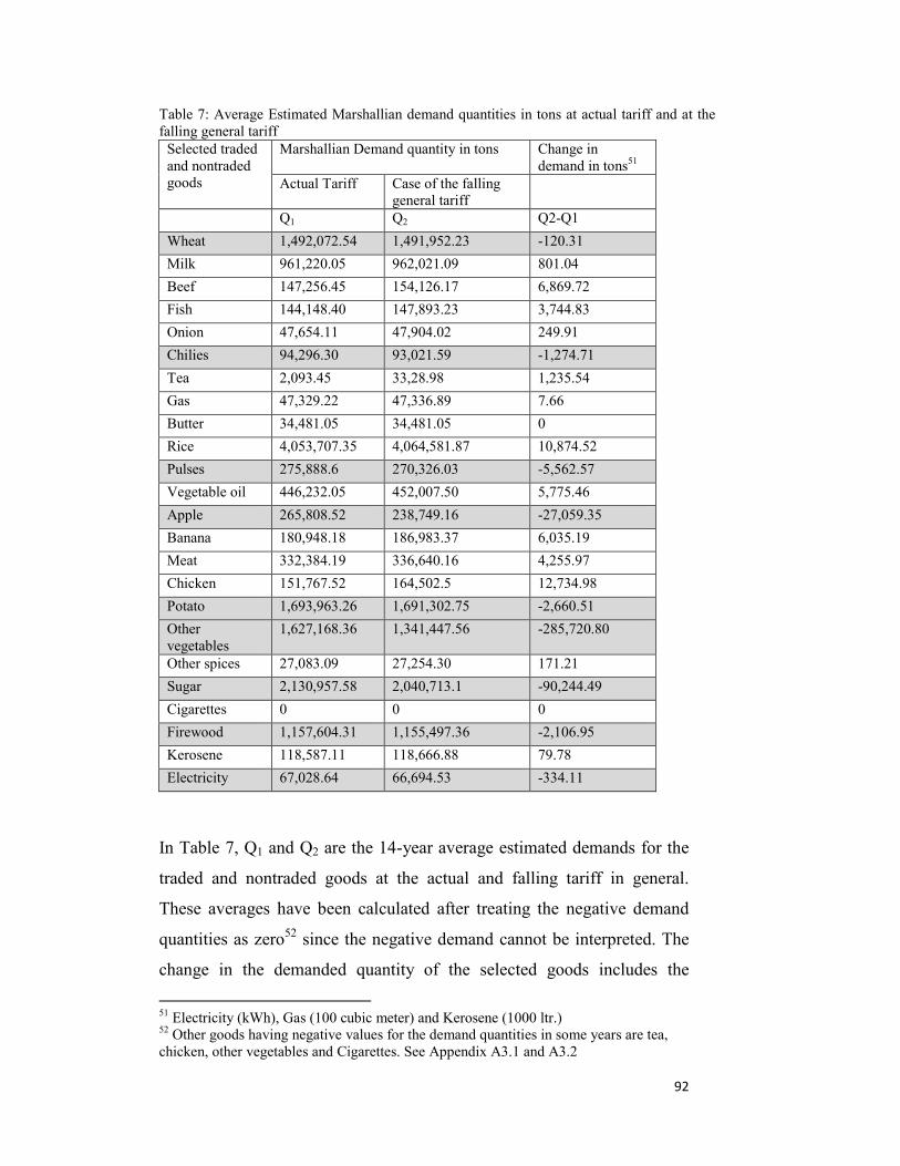
92

Table 7: Average Estimated Marshallian demand quantities in tons at actual tariff and at the falling general tariff

Selected traded and nontraded goods

Marshallian Demand quantity in tons Change in demand in tons51

Actual Tariff Case of the falling general tariff

Q1 Q2 Q2-Q1

Wheat 1,492,072.54 1,491,952.23 -120.31

Milk 961,220.05 962,021.09 801.04

Beef 147,256.45 154,126.17 6,869.72

Fish 144,148.40 147,893.23 3,744.83

Onion 47,654.11 47,904.02 249.91

Chilies 94,296.30 93,021.59 -1,274.71

Tea 2,093.45 33,28.98 1,235.54

Gas 47,329.22 47,336.89 7.66

Butter 34,481.05 34,481.05 0

Rice 4,053,707.35 4,064,581.87 10,874.52

Pulses 275,888.6 270,326.03 -5,562.57

Vegetable oil 446,232.05 452,007.50 5,775.46

Apple 265,808.52 238,749.16 -27,059.35

Banana 180,948.18 186,983.37 6,035.19

Meat 332,384.19 336,640.16 4,255.97

Chicken 151,767.52 164,502.5 12,734.98

Potato 1,693,963.26 1,691,302.75 -2,660.51

Other vegetables

1,627,168.36 1,341,447.56 -285,720.80

Other spices 27,083.09 27,254.30 171.21

Sugar 2,130,957.58 2,040,713.1 -90,244.49

Cigarettes 0 0 0

Firewood 1,157,604.31 1,155,497.36 -2,106.95

Kerosene 118,587.11 118,666.88 79.78

Electricity 67,028.64 66,694.53 -334.11

In Table 7, Q1 and Q2 are the 14-year average estimated demands for the

traded and nontraded goods at the actual and falling tariff in general.

These averages have been calculated after treating the negative demand

quantities as zero52 since the negative demand cannot be interpreted. The

change in the demanded quantity of the selected goods includes the

51 Electricity (kWh), Gas (100 cubic meter) and Kerosene (1000 ltr.) 52 Other goods having negative values for the demand quantities in some years are tea, chicken, other vegetables and Cigarettes. See Appendix A3.1 and A3.2

93

substitution and income effects of a price change. The reported rise in the

demanded quantity of the selected traded and nontraded goods is per the

expectations, however the reported average fall in the demand for wheat,

chilies, pulses, apple, potatoes, other vegetables, sugar, firewood and

electricity (shown in the light-shaded rows) need to be explained. In case

of wheat, chilies and apples their demands have reacted to the prices of

their substitutes such as rice, other spices and banana for each good

respectively. The households have partially substituted the demand for

these goods with cheaper substitutes. The demand for potatoes has

observed a fall because the households have partially substituted its

demand with onions and fall in its complementary good’s (other

vegetables) demand has caused decrease in its demand. In case of sugar, it

is expected from the positive sign of its own price coefficient that its

demand falls as its price falls. The demands for electricity has reported a

fall since its domestic price as a result of trade reform has increased and

demand for firewood has decreased since the households have substituted

it with kerosene and coal. In case of cigarettes, since its estimated demand

turns to be negative, it is treated as zero. The detailed tables on the

estimated Marshallian demand for all selected traded and nontraded goods

for all years at actual and the falling general tariff are provided in

Appendix A 3.1 and A 3.2.

5.3.3.2 Estimated Hicksian Demand

Marshallian demand functions presented in an earlier section include both

substitution and income effects of a price change on the quantity

demanded. Marshallian approach deals with cardinal utility functions

which does not distinguish between income and substitution effects of the

price change. Because the underlying utility functions of Pakistani

households are not known here therefore the Hicksian demand curves are

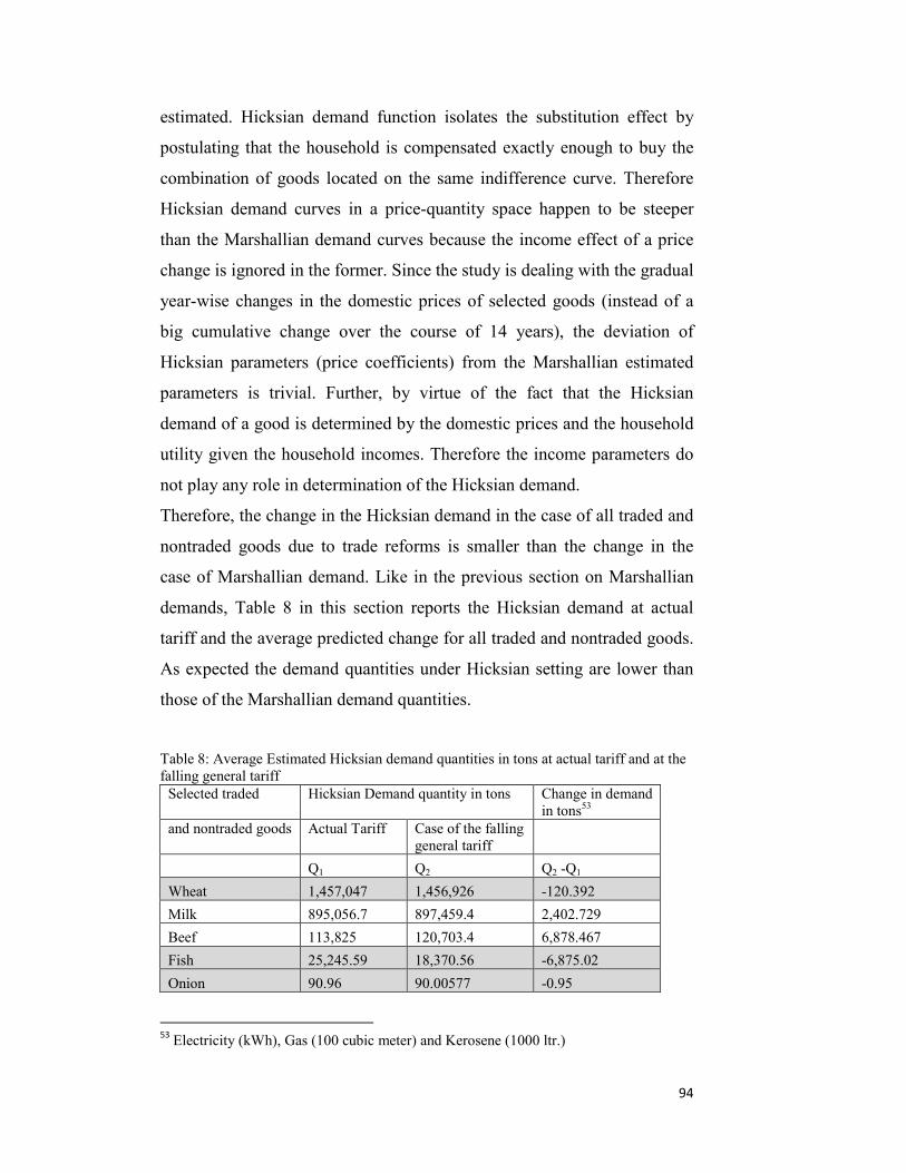
94

estimated. Hicksian demand function isolates the substitution effect by

postulating that the household is compensated exactly enough to buy the

combination of goods located on the same indifference curve. Therefore

Hicksian demand curves in a price-quantity space happen to be steeper

than the Marshallian demand curves because the income effect of a price

change is ignored in the former. Since the study is dealing with the gradual

year-wise changes in the domestic prices of selected goods (instead of a

big cumulative change over the course of 14 years), the deviation of

Hicksian parameters (price coefficients) from the Marshallian estimated

parameters is trivial. Further, by virtue of the fact that the Hicksian

demand of a good is determined by the domestic prices and the household

utility given the household incomes. Therefore the income parameters do

not play any role in determination of the Hicksian demand.

Therefore, the change in the Hicksian demand in the case of all traded and

nontraded goods due to trade reforms is smaller than the change in the

case of Marshallian demand. Like in the previous section on Marshallian

demands, Table 8 in this section reports the Hicksian demand at actual

tariff and the average predicted change for all traded and nontraded goods.

As expected the demand quantities under Hicksian setting are lower than

those of the Marshallian demand quantities.

Table 8: Average Estimated Hicksian demand quantities in tons at actual tariff and at the falling general tariff

Selected traded Hicksian Demand quantity in tons Change in demand in tons53

and nontraded goods Actual Tariff Case of the falling general tariff

Q1 Q2 Q2 -Q1

Wheat 1,457,047 1,456,926 -120.392

Milk 895,056.7 897,459.4 2,402.729

Beef 113,825 120,703.4 6,878.467

Fish 25,245.59 18,370.56 -6,875.02

Onion 90.96 90.00577 -0.95

53 Electricity (kWh), Gas (100 cubic meter) and Kerosene (1000 ltr.)

95

Chilies 65,954.74 64,680.01 -1,274.73

Tea 0 0 0

Gas 2,588.063 2,596.602 8.54

Butter 0 0 0

Rice 3,590,675 3,600,813 10,138.09

Pulses 479,263.4 473,702 -5,561.47

Vegetable oil 225,991.2 231,700 5,708.77

Apple 235,692.1 208,632.6 -27,059.6

Banana 92,491.86 98,525.64 6,033.776

Meat 45,291.96 48,785.15 3,493.192

Chicken 142,792.5 154,487.3 11,694.76

Potato 252,533.6 249,844.2 -2,689.35

Other vegetables 1,135,297 849,356.8 -285,940

Other spices 7,816.237 7,415.48 -400.76

Sugar 1,409,309 1,316,095 -93,214.2

Cigarettes 0 0 0

Firewood 734,909.4 732,802.4 -2,106.95

Kerosene 9,505.322 9,584.97 79.65

Electricity 32,017.03 31,682.92 -334.11

The Hicksian demand quantities are smaller than the Marshallian estimated

demand quantities. Once again, these averages of the Hicksian demand in

Table 8 are calculated after treating the negative demand quantities as zero

that may be produced by estimating the quantities on the bases of OLS-

estimates. In case of Hicksian demands, there are three goods which

reported negative estimated demand quantities during the whole period of

study (namely tea, butter and cigarettes). Further, it can be observed from

the Table 8 that now the change in the demand for two additional goods

(fish and other spices) is turning to be negative. In case of fish, the own

price elasticity is positive indicating that there can be other factors causing

a shift in its demand. As per the fish demand equation, the conventional

demand theory suggests that its demand should fall as its price falls. In the

presence of income effect in Marshallian approach the demand for fish

rose. However, under Hicksian approach, the removal of income effect

caused the decrease in the demand which is a case of fish as an absolute

96

inferior good. In case of other spices, the removal of income effect with

coefficient (0.74) almost double to its own price coefficient (-0.43) caused

a fall in its demand. See demand equations in Appendix A2. The detailed

table on estimated Hicksian demand for all selected traded and nontraded

goods for all years at actual and falling general tariff is provided in

Appendix A3.3 and A3.4.

5.4 Trade Liberalization, Household Welfare, Poorest Household Welfare and Labour incomes

This subsection is devoted to the interpretation of the empirical estimations

to investigate the effect of selective trade protectionist policy on the

household welfare. The adjustment in the welfare of the poorest households

in Pakistan owing to the trade reforms is discussed in the second part of the

section. The discussion is extended to the interpretation of the estimated

link between change in the labour incomes in agriculture and

manufacturing due to the selective protection in the last sections. Before

proceeding to the interpretations of the empirical outcomes on household

welfare, it is imperative to initiate the discussion on the issues related to the

Marshallian and Hicksian welfare measuring approaches. Following

subsection takes a detailed account on the two approaches.

5.4.1 Welfare Measuring Approaches

Welfare economics recommends consumer utility as the criterion for

measuring the consumer/household welfare. Since the utility is not readily

observable, therefore various welfare measuring criteria have always

remained controversial. Just (2004)54 has identified “not distinguishing

54 p. 98

97

between cardinality and ordinality of utility functions” as the key source

of the controversy. The cardinal system assumes that the utility can be

measured in quantitative terms i.e., in cardinal numbers such as 1, 2, 3 and

so on. Ordinal system on the other hand suggests that the utility cannot be

measured in quantitative units rather the utility drawn from different

combinations of goods can be ordered such that one is considered better,

worse or equal to the other by the consumers/households. Therefore the

utility is treated as subjective and it varies from person to person. Hence in

actual practice it cannot be measured in such quantitative or cardinal

terms. Marshallian Consumer Surplus is one welfare measure which

assumes the cardinality of the utility function. The concept of Consumer

Surplus was developed by Marshall (1930) and has formed since the basis

for most empirical welfare economic studies.55 Marshallian Consumer

Surplus has been criticized on many grounds such as its unrealistic

assumptions of independent utilities from each good,56 constant marginal

utility of money57 and interpersonal comparability58 (Mandal, 2007).59 To

cure these deficits Hicks (1939) proposes to measure people's willingness

to pay or willingness to accept to avoid a change in utility that would

follow a price change as their expression of welfare from a change of one

or of more than one price irrespective whether the underlying utility is

ordinal or cardinal. Compensating Variation is the amount of money

which, when taken away from an individual after a price change, leaves

the person just well off as before. Equivalent Variation is the amount of

money paid to an individual which, if price change does not happen,

leaves the individual just as well off as if the change had occurred. Just

55 p.6 56 This is so that Marshallian approach could not identify the case of substitute and complementary goods 57 This applies that there is no income effect of a price change and Giffen’s paradox when income effect turns negative and is stronger than the substitution effect 58 This applies that the utility of two individuals consuming the same good is comparable Just (2004) p. 4. 59 p. 14

98

(2004).60 Willig (1973, 1976) answered to the criticism on Consumer

Surplus by establishing firm theoretical relationship between two of the

Hicksian willingness to pay measures and the consumer surplus. Willig

approach suggested that Ordinary demand relationships can be used to

derive information about Hicksian compensated demands by using the

information they contain regarding income changes. Unfortunately Willig

approach is only valid for the variation of one price and for small income

changes and assumes a large error in consumer surplus if the income effect

is larger than 5% of the total price effect which is the upper bound for the

income effect of a price change. Just (2004)61. Hausman (1981) showed

how these Hicksian measures could be measured from compensated

demands using the market price and quantity data by deriving unobserved

compensated demands from observed market demands62.

Owing to the restrictive assumptions embedded in Marshallian approach

and the absence of information on the utility function of the Pakistani

households, our welfare measurement cannot only rely on the cardinal-

utility based approach. Further, since the Hicksian compensated demands

are not readily observable therefore the compensating variation is

measured from compensated demands driven from the information on

uncompensated (Marshallian) demands to measure the change in

household welfare. Slutsky equation is used to separate the income and

substitution effects from the total effect of a price change. Hausman

(1981) had the similar notion of measuring willingness to pay using

indirect utility and expenditure function.

60 p. 9 61 p.39 62 p.663

99

5.4.2 Marshallian Consumer Surplus (MCS)

Trade reforms initiate new domestic prices and consequently result in

different quantities demanded for all traded and nontraded household

consumption goods by varying proportions as elaborated in detail in the

previous sections. On average an ordinary Pakistani household loses from

the selective trade protectionist policy in the selected goods. As presented

in 4.2.4, the mathematical calculation of the MCS is the measurement of

the area under the uncompensated demand curve (P01P1

1ca in Figure 9b).

This can be calculated in two parts. In the first part, the change in the

estimated Marshallian demand is calculated by multiplying the estimated

Marshallian demand (Xi) with the trade reforms induced drop in the

estimated domestic prices (P01- P1

1) of selected traded and nontraded

goods. Secondly, change in the estimated Marshallian demand (X11-X0

1) is

multiplied by the trade reform induced drop in the estimated domestic

prices (P01- P1

1) of the selected goods and divided by two, because the area

under the demand curve is being measured. The summation of the two

effects i.e. 2

)X)(XP(P)P(PX

01

11

11

011

10

1i

−−+− would lead to the

measurement of the area (P01P1

1ca in 9b) or MCS with selective protection

and with liberalizing trend in general economy. This estimate is then

divided by the average number of households to calculate the households’

Marshallian Consumer Surplus.

The total loss under Marshallian Consumer Surplus in the all selected

goods and for all years is estimated at PKR 179.28 Billion (US

$3.82Billion)63 due to the selective protectionist policy in the selected

goods. See Table 9 for total loss over the period of 14 year in the selected

goods under Marshallian Consumer Surplus. According to the Table 9 the

selective protectionist policy has resulted in the loss in the consumers’

63 At the 14-year average exchange rate of PKR 46.885=1 US Dollar

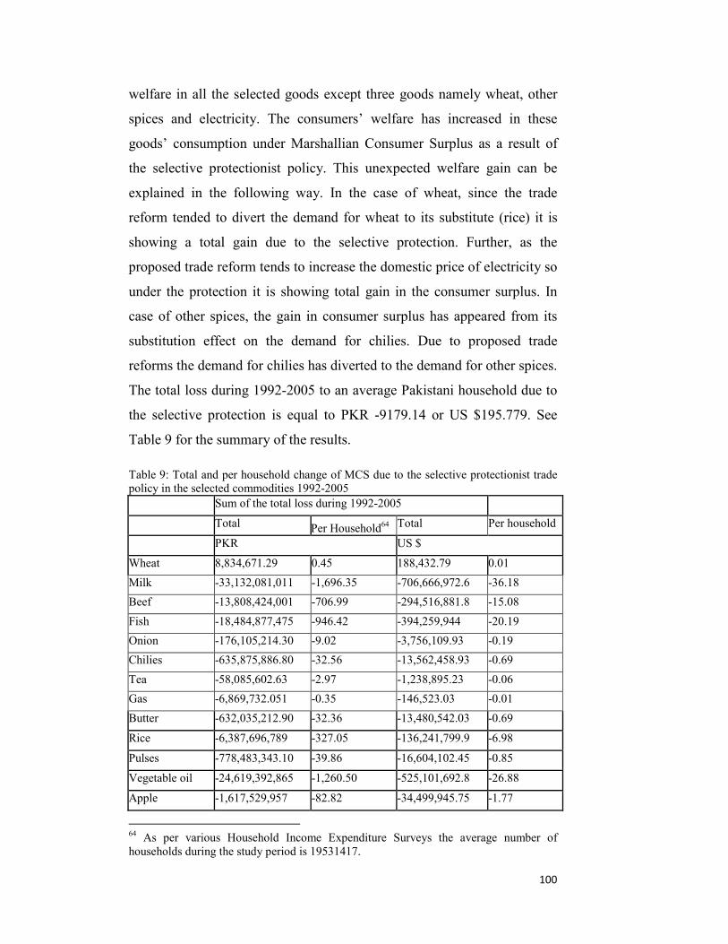
100

welfare in all the selected goods except three goods namely wheat, other

spices and electricity. The consumers’ welfare has increased in these

goods’ consumption under Marshallian Consumer Surplus as a result of

the selective protectionist policy. This unexpected welfare gain can be

explained in the following way. In the case of wheat, since the trade

reform tended to divert the demand for wheat to its substitute (rice) it is

showing a total gain due to the selective protection. Further, as the

proposed trade reform tends to increase the domestic price of electricity so

under the protection it is showing total gain in the consumer surplus. In

case of other spices, the gain in consumer surplus has appeared from its

substitution effect on the demand for chilies. Due to proposed trade

reforms the demand for chilies has diverted to the demand for other spices.

The total loss during 1992-2005 to an average Pakistani household due to

the selective protection is equal to PKR -9179.14 or US $195.779. See

Table 9 for the summary of the results.

Table 9: Total and per household change of MCS due to the selective protectionist trade policy in the selected commodities 1992-2005 Sum of the total loss during 1992-2005

Total Per Household64 Total Per household

PKR US $

Wheat 8,834,671.29 0.45 188,432.79 0.01

Milk -33,132,081,011 -1,696.35 -706,666,972.6 -36.18

Beef -13,808,424,001 -706.99 -294,516,881.8 -15.08

Fish -18,484,877,475 -946.42 -394,259,944 -20.19

Onion -176,105,214.30 -9.02 -3,756,109.93 -0.19

Chilies -635,875,886.80 -32.56 -13,562,458.93 -0.69

Tea -58,085,602.63 -2.97 -1,238,895.23 -0.06

Gas -6,869,732.051 -0.35 -146,523.03 -0.01

Butter -632,035,212.90 -32.36 -13,480,542.03 -0.69

Rice -6,387,696,789 -327.05 -136,241,799.9 -6.98

Pulses -778,483,343.10 -39.86 -16,604,102.45 -0.85

Vegetable oil -24,619,392,865 -1,260.50 -525,101,692.8 -26.88

Apple -1,617,529,957 -82.82 -34,499,945.75 -1.77

64 As per various Household Income Expenditure Surveys the average number of households during the study period is 19531417.

101

Banana -1,238,706,379 -63.42 -26,420,099.79 -1.35

Meat 3,920,876,641 200.75 83,627,527.8 4.28

Chicken -42,622,207,784 -2,182.24 -909,079,829 -46.54

Potato -400,742,684.50 -20.52 -8,547,353.84 -0.44

Other vegetables -4,104,470,248 -210.15 -87,543,356.03 -4.48

Other spices 103,623,333.40 5.31 2,210,159.61 0.11

Sugar -34,350,221,411 -1,758.72 -732,648,425.1 -37.51

Cigarettes 0 0 0 0

Firewood -163,025.27 -0.01 -3,477.13 -0.0002

Kerosene -260,983,220.40 -13.36 -5,566,454.52 -0.28

Electricity 33.77 0.000002 0.72 0.00000004

Total -179,281,617,161.35 -9,179.14 -3,823,858,742.91 -195.78

The detailed information on the estimated annual loss in MCS in all

selected goods for all years is provided in Appendix A5.1. The average

yearly loss to an ordinary household is equal to PKR -655.65. See Table

10 for the summary of the results on the yearly total and average loss

under MCS to the ordinary Pakistani households.

Table 10: Yearly total and average change in MCS of the ordinary Pakistani household Total Loss Loss per ordinary household

PKR US $ PKR US $

1992 -11,904 -458.54 -0.001 0.0000

1993 -1,579,683,166 -52,376,762.81 -80.88 -2.68

1994 1,318,296,437 42,732,461.50 67.5 2.19

1995 -292,269,007 -8,706,255.79 -14.96 -0.45

1996 -3,139,296,095 -80,515,416.65 -160.73 -4.12

1997 -16,113,745,316 -373,089,727.16 -825.02 -19.1

1998 -155,247,932,103 -3,317,972,474.95 -7,948.63 -169.88

1999 3,097,265,195 59,827,413.46 158.58 3.06

2000 -1,878,629,195 -32,146,290.12 -96.18 -1.65

2001 -5,051,864,299 -82,237,738.88 -258.65 -4.21

2002 -11,028,252,331 -188,517,133.86 -564.64 -9.65

2003 -23,639,133,390 -410,615,483.58 -1,210.31 -21.02

2004 1,533,190,428 25,837,385.04 78.5 1.32

2005 32,740,447,584 547,224,596.09 1,676.3 28.02

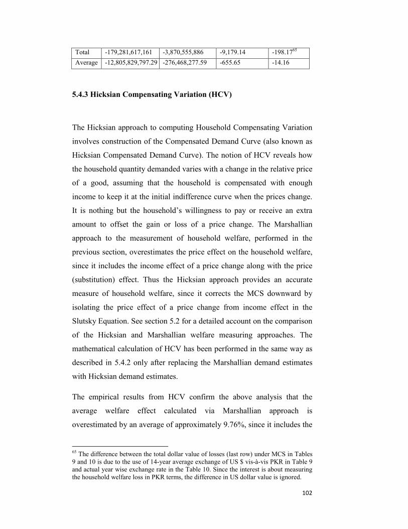
102

Total -179,281,617,161 -3,870,555,886 -9,179.14 -198.1765

Average -12,805,829,797.29 -276,468,277.59 -655.65 -14.16

5.4.3 Hicksian Compensating Variation (HCV)

The Hicksian approach to computing Household Compensating Variation

involves construction of the Compensated Demand Curve (also known as

Hicksian Compensated Demand Curve). The notion of HCV reveals how

the household quantity demanded varies with a change in the relative price

of a good, assuming that the household is compensated with enough

income to keep it at the initial indifference curve when the prices change.

It is nothing but the household’s willingness to pay or receive an extra

amount to offset the gain or loss of a price change. The Marshallian

approach to the measurement of household welfare, performed in the

previous section, overestimates the price effect on the household welfare,

since it includes the income effect of a price change along with the price

(substitution) effect. Thus the Hicksian approach provides an accurate

measure of household welfare, since it corrects the MCS downward by

isolating the price effect of a price change from income effect in the

Slutsky Equation. See section 5.2 for a detailed account on the comparison

of the Hicksian and Marshallian welfare measuring approaches. The

mathematical calculation of HCV has been performed in the same way as

described in 5.4.2 only after replacing the Marshallian demand estimates

with Hicksian demand estimates.

The empirical results from HCV confirm the above analysis that the

average welfare effect calculated via Marshallian approach is

overestimated by an average of approximately 9.76%, since it includes the

65 The difference between the total dollar value of losses (last row) under MCS in Tables 9 and 10 is due to the use of 14-year average exchange of US $ vis-à-vis PKR in Table 9 and actual year wise exchange rate in the Table 10. Since the interest is about measuring the household welfare loss in PKR terms, the difference in US dollar value is ignored.

103

income effect of a price change. The total national figure for the gain

under HCV is estimated at PKR 161.78 Billion (US $ 3.45 Billion) as a

result of a selective protectionist policy in the selected goods. See Table

11 for total loss over the period of 14 year in the selected goods under

Hicksian Compensating Approach. Quiet in line with the MCS, the

consumers have gained in the consumption of three goods namely wheat,

other spices and electricity. The rationale for the welfare gain in the three

goods given in 5.2.1 can be referred to here.

Table 11: Total and per household change of HCV due to the selective protectionist trade policy in the selected commodities 1992-2005

Sum of the loss during 1992-2005 Total Per Household66 Total Per household PKR US $ Wheat 8,602,432.11 0.44 183,479.41 0.01 Milk -30,290,487,679 -1,550.86 -646,059,244.5 -33.08 Beef -17,537,284,785 -897.90 -374,048,945 -19.15 Fish -14,439,906,736 -739.32 -307,985,640.1 -15.77 Onion -177,101.74 -0.01 -3,777.36 -0.0002 Chilies -440,393,619.4 -22.55 -9,393,060.03 -0.48 Tea 0 0 0 0 Gas -256,988.29 -0.013 -5,481.25 -0.0003 Butter 0 0 0 0 Rice -5,678,069,739 -290.71 -121,106,318.4 -6.20 Pulses -893,933,319.7 -45.769 -19,066,509.97 -0.98 Vegetable oil -9,949,274,701 -509.4 -212,205,923 -10.86 Apple -1,409,804,940 -72.18 -30,069,423.92 -1.54 Banana -628,574,054.8 -32.18 -13,406,719.74 -0.69 Meat -11,255,524,292 -576.28 -240,066,637.3 -12.29 Chicken -42,800,668,737 -2,191.38 -912,886,184 -46.74 Potato -297,420,699.8 -15.23 -6,343,621.62 -0.32 Other vegetables -3,029,497,127 -155.11 -64,615,487.4 -3.31 Other spices 129,233,343.8 6.62 2,756,389.97 0.14 Sugar -23,246,869,990 -1,190.23 -495,827,449.9 -25.39 Cigarettes 0 0 0 00 Firewood -97,435.5 -0.005 -2078.18 -0.0001 Kerosene -19,616,272.34 -1.0043 -418,391.22 -0.02 Electricity 15.58 0.000001 0.33 0.000000 Total -161,780,022,427.64 -8,283.07 -3,450,571,023 -176.67

The total loss in the welfare of the ordinary households during 1992-2005

is equal to PKR -8283.07 and the average yearly loss is equal to PKR -

66 As per various Household Income Expenditure Surveys the average number of households during the study period is 19531417.

104

591.65. The yearly total and average loss under HCV is presented in the

following Table 12. The detailed information on the loss in the estimated

Compensating Variation in all selected goods for all years is provided in

Appendix A5.2.

Table 12: Yearly total change in HCV and change in HCV per average Pakistani household Total Loss Loss per ordinary household

PKR US $ PKR US $

1992 -12,190 -469.56 -0.001 -0.000024 1993 -826,488,048 -27,403,449.86 -42.32 -1.40 1994 673,033,766 21,816,329.52 34.46 1.12 1995 -161,816,812 -4,820,280.38 -8.28 -0.25 1996 -1,959,030,099 -50,244,424.19 -100.30 -2.57 1997 -8,291,752,362 -191,983,152.6 -424.53 -9.83 1998 -114,055,677,506 -2,437,607,983 -5839.60 -124.80 1999 -8,539,619,492 -164,953,051.8 -437.22 -8.45 2000 -9,620,935,195 -164,629,281.2 -492.59 -8.43 2001 -3,515,841,494 -57,233,297.97 -180.01 -2.93 2002 -6,667,186,055 -113,968,992.4 -341.36 -5.84 2003 -15,307,313,011 -265,890,446.6 -783.73 -13.61 2004 3,699,666,756 62,346,928.81 189.42 3.19 2005 2,792,949,316 46,681,419.28 143 2.39 Total -161,780,022,428 -3,347,890,152 -8,283.06 -171.4167

Average -11,555,715,887.57 -239,135,010.85 -591.65 -12.24

The comparative analysis of the estimations of the two household welfare

approaches suggests that both MCS and HCV approaches reflect a loss in

the household welfare due to a selective protectionist trade policy.

However, a close comparison of the two measures reveals the importance

of using both approaches instead of a single approach (MCS) in the study.

The following Table 13 presents the comparison of the estimated welfare

losses under the two approaches.

67 The difference between the total dollar value of losses (last row) under HCV in Tables 11 and 12 is due to the use of 14-year average exchange of US $ vis-à-vis PKR in Table 11 and actual year wise exchange rate in Table 12. Since the interest is about measuring the household welfare loss in PKR terms, the difference in US dollar value is ignored.

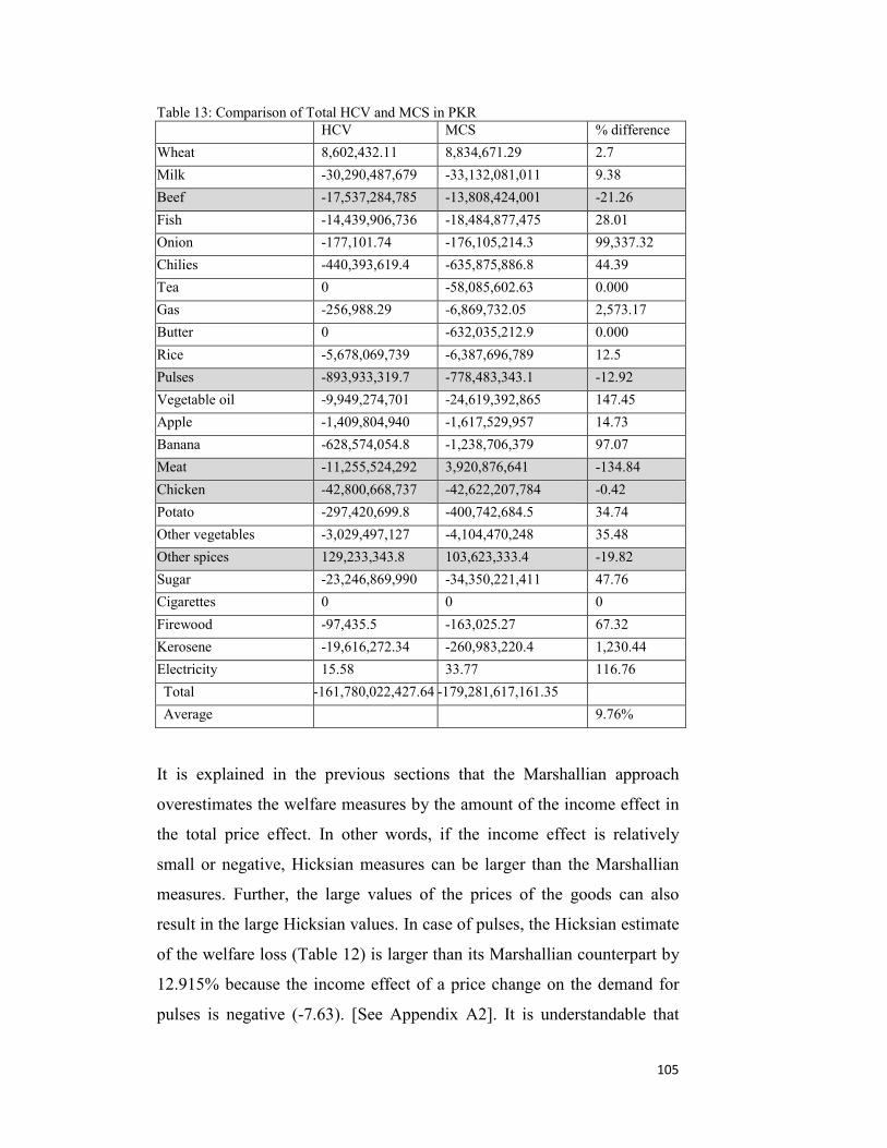
105

Table 13: Comparison of Total HCV and MCS in PKR HCV MCS % difference

Wheat 8,602,432.11 8,834,671.29 2.7

Milk -30,290,487,679 -33,132,081,011 9.38

Beef -17,537,284,785 -13,808,424,001 -21.26

Fish -14,439,906,736 -18,484,877,475 28.01

Onion -177,101.74 -176,105,214.3 99,337.32

Chilies -440,393,619.4 -635,875,886.8 44.39

Tea 0 -58,085,602.63 0.000

Gas -256,988.29 -6,869,732.05 2,573.17

Butter 0 -632,035,212.9 0.000

Rice -5,678,069,739 -6,387,696,789 12.5

Pulses -893,933,319.7 -778,483,343.1 -12.92

Vegetable oil -9,949,274,701 -24,619,392,865 147.45

Apple -1,409,804,940 -1,617,529,957 14.73

Banana -628,574,054.8 -1,238,706,379 97.07

Meat -11,255,524,292 3,920,876,641 -134.84

Chicken -42,800,668,737 -42,622,207,784 -0.42

Potato -297,420,699.8 -400,742,684.5 34.74

Other vegetables -3,029,497,127 -4,104,470,248 35.48

Other spices 129,233,343.8 103,623,333.4 -19.82

Sugar -23,246,869,990 -34,350,221,411 47.76

Cigarettes 0 0 0

Firewood -97,435.5 -163,025.27 67.32

Kerosene -19,616,272.34 -260,983,220.4 1,230.44

Electricity 15.58 33.77 116.76

Total -161,780,022,427.64 -179,281,617,161.35

Average 9.76%

It is explained in the previous sections that the Marshallian approach

overestimates the welfare measures by the amount of the income effect in

the total price effect. In other words, if the income effect is relatively

small or negative, Hicksian measures can be larger than the Marshallian

measures. Further, the large values of the prices of the goods can also

result in the large Hicksian values. In case of pulses, the Hicksian estimate

of the welfare loss (Table 12) is larger than its Marshallian counterpart by

12.915% because the income effect of a price change on the demand for

pulses is negative (-7.63). [See Appendix A2]. It is understandable that

106

when the (negative) income effect from the total price change is excluded,

the Hicksian measure would produce a large value for the welfare loss.

Further, in case of beef, meat, chicken and other spices, the relatively large

values of their prices (per ton) cause the Hicksian measure (due to

exclusion of the income effect) to be larger than the Marshallian measures.

The domestic prices of beef at actual tariff (PKR 70,699.17 per ton), Meat

(PKR 122,005.81 per ton), Chicken (PKR 79,774.07 per ton) and other

spices (PKR 42,219.49 per ton) are relatively larger than the domestic

prices of other goods. The domestic prices of all other goods are less than

PKR 10,000 per ton except milk (PKR 24055.88 per ton), Fish (PKR

61290.72 per ton), chilies (PKR 20646.18 per ton), tea (PKR 64800.75),

Butter (PKR 50768.44 per ton), vegetable oil (PKR 40013.46 per ton) and

cigarettes (PKR 2665610.71 per ton). [See Table 1 for the domestic prices

of selected goods at actual and at the falling general tariff]. Amongst, the

HCV and MCS welfare measures cannot be compared for tea, butter and

cigarettes as the estimated demands for these goods under Hicksian

approach turn to be negative which cannot be interpreted. (See A 3.3 and

A3.4 for Hicksian demands). In addition, some goods as onion

(99337.315%), gas (2573.169%) and kerosene (1230.442%) depict large

differences between Hicksian and Marshallian welfare losses. This is

because of the exclusion of the relatively larger income effect than the

own price coefficients in the case of onion and gas [(log-linear income

coefficients in onion and gas are (0.67) and (0.516) and the price

coefficients are (-0.064) and (-0.054) respectively] and due to the large

complementary effect of the price of electricity (-5117.39) in linear

demand equation of kerosene. Another reason for the large difference

between HCV and MCS in case of onion is its negative estimated Hicksian

demand in most of the years (and treated as zero) therefore the welfare

loss under HCV is suppressed in relation to the loss under MCS.

Further, according to the above Table 13 the MCS overestimates the total

welfare loss calculated from the average values (PKR -

107

179,281,617,161.35) by 9.76% than the welfare loss under HCV

calculated from the average values (PKR -161,780,022,427.64) which

defies the upper bound of 5%, proposed in Willig (1973) to approximate

the MCS with the willingness to pay approach. Further the differences

between the Hicksian and the Marshallian losses are too large in case of

onion, gas and kerosene. [See Table 13]. Therefore the estimation of the

welfare loss under the Hicksian measure is taken to be more accurate than

the Marshallian measure and the Willig (1973) proposal of relying on

MCS as a suitable welfare measure is not accepted here.

5.4.4 Poorest Households’ Demand and Welfare (MCS)

In absence of the data on the poorest household consumption patterns,

their demand quantities have been calculated from the budget shares of the

poorest households allocated for various goods and the calculated

domestic prices (including actual and falling general tariffs separately to

obtain budget shares at both tariffs) in the following way. As presented in

4.2.5, the above setting is justified only under Cobb-Douglas utility

function which assumes that despite price changes the budget share in a

given year does not change.

YXP

S iii = (44)

Rearranging equation (44) for demand:

i

ii P

YSX = (45)

Here s is the households’ budget share (in percentage) allocated for a

good, Pi is the vector of the domestic prices (including tariff) of the goods,

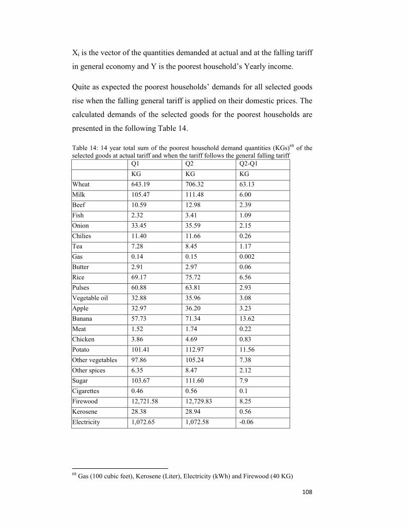
108

Xi is the vector of the quantities demanded at actual and at the falling tariff

in general economy and Y is the poorest household’s Yearly income.

Quite as expected the poorest households’ demands for all selected goods

rise when the falling general tariff is applied on their domestic prices. The

calculated demands of the selected goods for the poorest households are

presented in the following Table 14.

Table 14: 14 year total sum of the poorest household demand quantities (KGs)68 of the selected goods at actual tariff and when the tariff follows the general falling tariff Q1 Q2 Q2-Q1

KG KG KG

Wheat 643.19 706.32 63.13

Milk 105.47 111.48 6.00

Beef 10.59 12.98 2.39

Fish 2.32 3.41 1.09

Onion 33.45 35.59 2.15

Chilies 11.40 11.66 0.26

Tea 7.28 8.45 1.17

Gas 0.14 0.15 0.002

Butter 2.91 2.97 0.06

Rice 69.17 75.72 6.56

Pulses 60.88 63.81 2.93

Vegetable oil 32.88 35.96 3.08

Apple 32.97 36.20 3.23

Banana 57.73 71.34 13.62

Meat 1.52 1.74 0.22

Chicken 3.86 4.69 0.83

Potato 101.41 112.97 11.56

Other vegetables 97.86 105.24 7.38

Other spices 6.35 8.47 2.12

Sugar 103.67 111.60 7.9

Cigarettes 0.46 0.56 0.1

Firewood 12,721.58 12,729.83 8.25

Kerosene 28.38 28.94 0.56

Electricity 1,072.65 1,072.58 -0.06

68 Gas (100 cubic feet), Kerosene (Liter), Electricity (kWh) and Firewood (40 KG)

109

The demand for all selected goods observes a positive change with the

tariff included domestic prices following the falling general tariff instead

of the actual tariff (see Q2-Q1 in Table 14) except electricity as its price

has increased as a result of proposed trade reform. The poorest households

demand more of all commodities (except electricity) as they perceive a

drop in the domestic prices due to tariff cuts. As in real world, the tariff

rate on the selected goods is escalating (selective protectionist policy),

therefore the predicted rise in the quantity demanded of all goods in Table

14 is indeed the loss in the poorest households’ demand due to the

protection. Following Table 15 presents the predicted loss in the single

poorest household’s welfare under MCS for all years and in all goods due

to the selective protectionist trade policy.

Table 15: Single poorest household’s change in MCS due to the selective protectionist trade policy 1992-2005 Poorest household’s loss under MCS

PKR US $69

Wheat -5,360.68 -114.34

Milk -1,973.67 -42.10

Beef -1,220.11 -26.02

Fish -222.65 -4.75

Onion -205.58 -4.38

Chilies -66.69 -1.42

Tea -815.29 -17.39

Gas -15.38 -0.33

Butter -51.70 -1.10

Rice -728.76 -15.54

Pulses -338.55 -7.22

Vegetable oil -1347.75 -28.75

Apple -207.63 -4.43

Banana -342.25 -7.30

Meat -248.59 -5.30

Chicken -630.75 -13.45

Potato -530.77 -11.32

Other vegetables -574.48 -12.25

Other spices -617.55 -13.17

Sugar -970.87 -20.71

69 Calculated at 1992-2005 average Exchange Rate

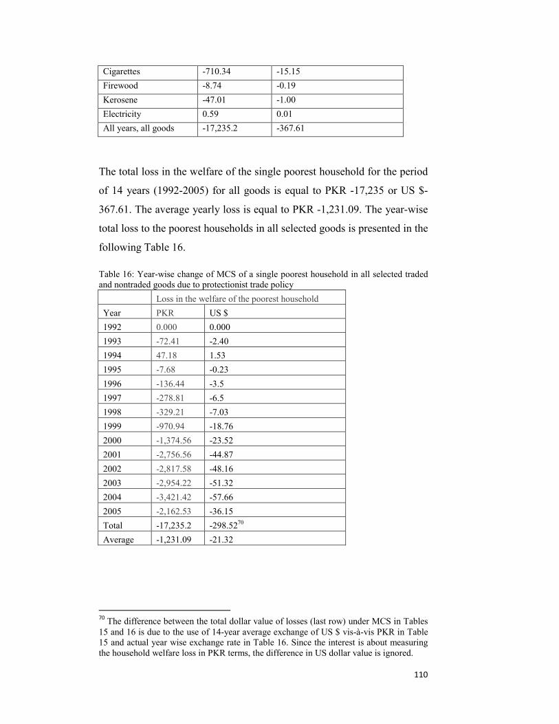
110

Cigarettes -710.34 -15.15

Firewood -8.74 -0.19

Kerosene -47.01 -1.00

Electricity 0.59 0.01

All years, all goods -17,235.2 -367.61

The total loss in the welfare of the single poorest household for the period

of 14 years (1992-2005) for all goods is equal to PKR -17,235 or US $-

367.61. The average yearly loss is equal to PKR -1,231.09. The year-wise

total loss to the poorest households in all selected goods is presented in the

following Table 16.

Table 16: Year-wise change of MCS of a single poorest household in all selected traded and nontraded goods due to protectionist trade policy

Loss in the welfare of the poorest household

Year PKR US $

1992 0.000 0.000

1993 -72.41 -2.40

1994 47.18 1.53

1995 -7.68 -0.23

1996 -136.44 -3.5

1997 -278.81 -6.5

1998 -329.21 -7.03

1999 -970.94 -18.76

2000 -1,374.56 -23.52

2001 -2,756.56 -44.87

2002 -2,817.58 -48.16

2003 -2,954.22 -51.32

2004 -3,421.42 -57.66

2005 -2,162.53 -36.15

Total -17,235.2 -298.5270

Average -1,231.09 -21.32

70 The difference between the total dollar value of losses (last row) under MCS in Tables 15 and 16 is due to the use of 14-year average exchange of US $ vis-à-vis PKR in Table 15 and actual year wise exchange rate in Table 16. Since the interest is about measuring the household welfare loss in PKR terms, the difference in US dollar value is ignored.

111

The detailed Table on the loss in the poorest households’ consumer

surplus in all traded and nontraded goods for all years due to the selective

protectionist trade policy is presented in Appendix A5.3.

5.5 Labour Incomes and the Domestic Prices of the Selected Goods

The labour income and the price relationship is estimated in log-linear for

tune to the equation 38

∂∂

+= ∑=

ii

iii

n

1i0i L

LQ

Pαlnlnαlnw in agriculture

and manufacturing. The data on the labour allocation in the production of

each good is not available in the labour force surveys. Two methods then

remain open for the estimation of the link between labour income and the

domestic prices. Either the total agriculture or manufacturing labour

should be used with the domestic prices of agriculture and manufacturing

goods in the estimation of the link. However it would produce the

exaggerated results on the labour income from the production of each

good by the number of the selected goods in each sector. Because it would

inherently be assumed that all agriculture or manufacturing labour is

allocated in the production of each single good in both sectors. Another

way is to calculate the labour allocation in the production of each good by

approximating it with the percentage share of each good in the total

agriculture or manufacturing production. If, for example, the production of

wheat is 16.54% of the total agriculture production then 16.54% of the

total labour employed in agriculture should be assumed to be allocated in

the wheat production and so on. The similar approximation may apply for

the labour employment in the production of the selected manufactured

goods. Though in this method, the underlying assumption of equal

marginal productivity of labour in the production of each good may not be

true. Nevertheless in absence of the accurate data on labour allocation in

the production of each good, this method can produce results which are

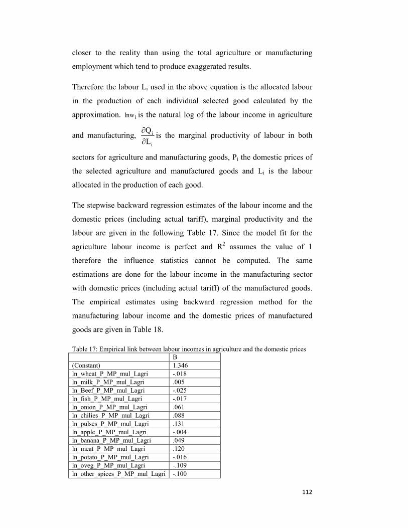
112

closer to the reality than using the total agriculture or manufacturing

employment which tend to produce exaggerated results.

Therefore the labour Li used in the above equation is the allocated labour

in the production of each individual selected good calculated by the

approximation. ilnw is the natural log of the labour income in agriculture

and manufacturing, i

i

LQ∂∂

is the marginal productivity of labour in both

sectors for agriculture and manufacturing goods, Pi the domestic prices of

the selected agriculture and manufactured goods and Li is the labour

allocated in the production of each good.

The stepwise backward regression estimates of the labour income and the

domestic prices (including actual tariff), marginal productivity and the

labour are given in the following Table 17. Since the model fit for the

agriculture labour income is perfect and R2 assumes the value of 1

therefore the influence statistics cannot be computed. The same

estimations are done for the labour income in the manufacturing sector

with domestic prices (including actual tariff) of the manufactured goods.

The empirical estimates using backward regression method for the

manufacturing labour income and the domestic prices of manufactured

goods are given in Table 18.

Table 17: Empirical link between labour incomes in agriculture and the domestic prices B (Constant) 1.346 ln_wheat_P_MP_mul_Lagri -.018 ln_milk_P_MP_mul_Lagri .005 ln_Beef_P_MP_mul_Lagri -.025 ln_fish_P_MP_mul_Lagri -.017 ln_onion_P_MP_mul_Lagri .061 ln_chilies_P_MP_mul_Lagri .088 ln_pulses_P_MP_mul_Lagri .131 ln_apple_P_MP_mul_Lagri -.004 ln_banana_P_MP_mul_Lagri .049 ln_meat_P_MP_mul_Lagri .120 ln_potato_P_MP_mul_Lagri -.016 ln_oveg_P_MP_mul_Lagri -.109 ln_other_spices_P_MP_mul_Lagri -.100

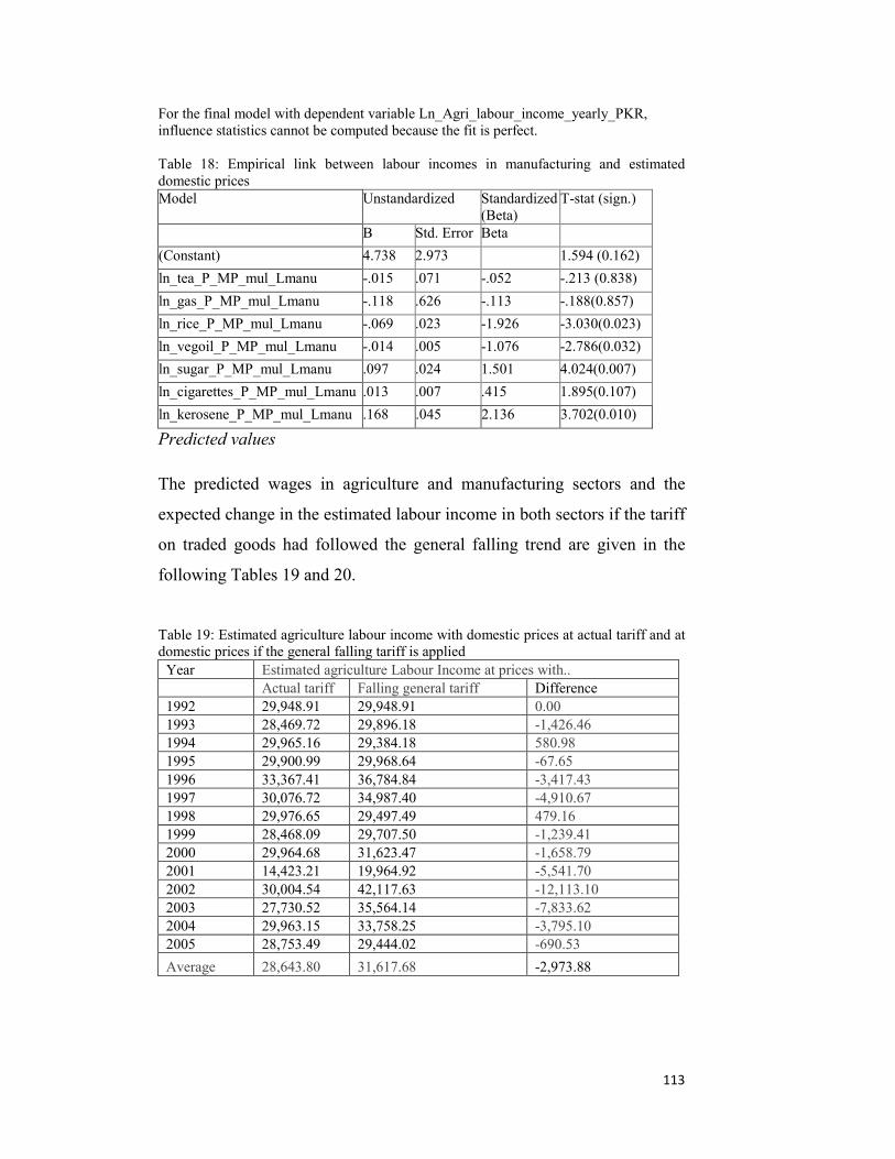
113

For the final model with dependent variable Ln_Agri_labour_income_yearly_PKR, influence statistics cannot be computed because the fit is perfect. Table 18: Empirical link between labour incomes in manufacturing and estimated domestic prices Model Unstandardized Standardized

(Beta) T-stat (sign.)

B Std. Error Beta

(Constant) 4.738 2.973 1.594 (0.162)

ln_tea_P_MP_mul_Lmanu -.015 .071 -.052 -.213 (0.838)

ln_gas_P_MP_mul_Lmanu -.118 .626 -.113 -.188(0.857)

ln_rice_P_MP_mul_Lmanu -.069 .023 -1.926 -3.030(0.023)

ln_vegoil_P_MP_mul_Lmanu -.014 .005 -1.076 -2.786(0.032)

ln_sugar_P_MP_mul_Lmanu .097 .024 1.501 4.024(0.007)

ln_cigarettes_P_MP_mul_Lmanu .013 .007 .415 1.895(0.107)

ln_kerosene_P_MP_mul_Lmanu .168 .045 2.136 3.702(0.010)

Predicted values

The predicted wages in agriculture and manufacturing sectors and the

expected change in the estimated labour income in both sectors if the tariff

on traded goods had followed the general falling trend are given in the

following Tables 19 and 20.

Table 19: Estimated agriculture labour income with domestic prices at actual tariff and at domestic prices if the general falling tariff is applied

Year Estimated agriculture Labour Income at prices with.. Actual tariff Falling general tariff Difference 1992 29,948.91 29,948.91 0.00 1993 28,469.72 29,896.18 -1,426.46 1994 29,965.16 29,384.18 580.98 1995 29,900.99 29,968.64 -67.65 1996 33,367.41 36,784.84 -3,417.43 1997 30,076.72 34,987.40 -4,910.67 1998 29,976.65 29,497.49 479.16 1999 28,468.09 29,707.50 -1,239.41 2000 29,964.68 31,623.47 -1,658.79 2001 14,423.21 19,964.92 -5,541.70 2002 30,004.54 42,117.63 -12,113.10 2003 27,730.52 35,564.14 -7,833.62 2004 29,963.15 33,758.25 -3,795.10 2005 28,753.49 29,444.02 -690.53

Average 28,643.80 31,617.68 -2,973.88

114

Compare the estimated labour income in agriculture at domestic prices at

actual and the falling general tariff in the Table 19. The estimated

agriculture labour income is predicted to rise in all years except 1994 and

1998. As the year 1992 is the base year for the calculation of the tariff

rates, the difference in labour income in this year is zero (see Section

5.1.1). In 1994, the general tariff rate has increased instead of falling

which has reversed the relation between the domestic prices and wages.

The last column on the right in Table 18 reports the difference in the

estimated labour income in agriculture sector at actual and at the falling

general tariff. The negative values in this column confirm the loss in the

agriculture labour income due to the selective protection in the selected

commodities. On average the agriculture labour has suffered a yearly loss

of -2973.88 PKR71. The average labour income in agriculture is predicted

to have risen from 28643.80 PKR to 31617.68 PKR per year. In

comparison to the average yearly loss in the MCS per household (PKR

9179.14) and the loss in the HCV per household (PKR 8283), the

predicted loss in the agriculture labour income is modest. One possible

explanation for the relatively small predicted loss (or expected benefit of

the trade reforms) in agriculture labour incomes due to the proposed trade

reforms can be attributed to the highly skewed land ownership in the

country. The feudal archetype in Pakistan consists of the landlords

possessing thousands of acres of agricultural land. About 67% of

households own no land in the country. Unusually, just 0.3% households

own 55 or more acres of land across the country, suggesting a highly

skewed land ownership pattern72. The studies also argue that the skewed

land distribution results in patterns of sharecropping that exploit poor

tenants. It is a fact that most of the agriculture sector in the country is

71 The labour income in agriculture sector was predicted to increase by this amount if the selected commodities had been priced at the falling general tariff instead of the escalating actual tariff (trade reforms instead of the selective protection) 72 World Bank (2002)

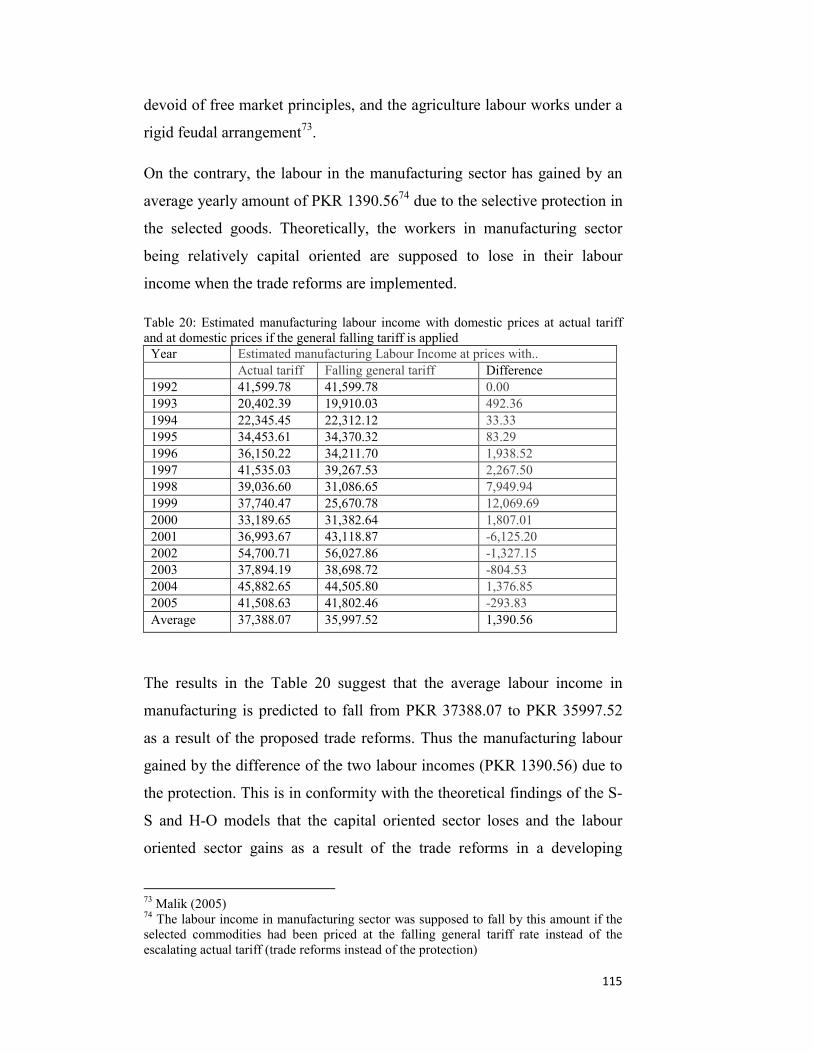
115

devoid of free market principles, and the agriculture labour works under a

rigid feudal arrangement73.

On the contrary, the labour in the manufacturing sector has gained by an

average yearly amount of PKR 1390.5674 due to the selective protection in

the selected goods. Theoretically, the workers in manufacturing sector

being relatively capital oriented are supposed to lose in their labour

income when the trade reforms are implemented.

Table 20: Estimated manufacturing labour income with domestic prices at actual tariff and at domestic prices if the general falling tariff is applied

Year Estimated manufacturing Labour Income at prices with.. Actual tariff Falling general tariff Difference 1992 41,599.78 41,599.78 0.00 1993 20,402.39 19,910.03 492.36 1994 22,345.45 22,312.12 33.33 1995 34,453.61 34,370.32 83.29 1996 36,150.22 34,211.70 1,938.52 1997 41,535.03 39,267.53 2,267.50 1998 39,036.60 31,086.65 7,949.94 1999 37,740.47 25,670.78 12,069.69 2000 33,189.65 31,382.64 1,807.01 2001 36,993.67 43,118.87 -6,125.20 2002 54,700.71 56,027.86 -1,327.15 2003 37,894.19 38,698.72 -804.53 2004 45,882.65 44,505.80 1,376.85 2005 41,508.63 41,802.46 -293.83 Average 37,388.07 35,997.52 1,390.56

The results in the Table 20 suggest that the average labour income in

manufacturing is predicted to fall from PKR 37388.07 to PKR 35997.52

as a result of the proposed trade reforms. Thus the manufacturing labour

gained by the difference of the two labour incomes (PKR 1390.56) due to

the protection. This is in conformity with the theoretical findings of the S-

S and H-O models that the capital oriented sector loses and the labour

oriented sector gains as a result of the trade reforms in a developing

73 Malik (2005) 74 The labour income in manufacturing sector was supposed to fall by this amount if the selected commodities had been priced at the falling general tariff rate instead of the escalating actual tariff (trade reforms instead of the protection)

116

country setting and vice versa in case of protectionist policy. In the case of

Pakistan, the agriculture sector employs unskilled workers intensively

therefore gains in terms of rise in the labor incomes; the manufacturing

sector, being relatively capital intensive since it employs machinery, loses

in terms of fall in the labour income as a result of trade reforms.

Implications of the Labour income-domestic Prices Link

The major employment sectors for both categories of workers (skilled and

unskilled) reported in various Labor Force Surveys published by the

Statistics Division of Pakistan are agriculture; manufacturing;

construction; and wholesale and retail trade and hotel and restaurants.

These four sectors cover 81.13% (36 year-average) of the total employed

labor force of the country. Other sectors are mining and quarrying,

electricity, gas and water, transport, storage and communication, finance,

insurance, real estate and business services, community, social and

personal services, and activities not adequately defined, which provide a

livelihood to the remaining 19% of total employed labor force. Sector-

wise average percentage employment of the total employed labor force is

as follows: agriculture (51%), manufacturing (13%), construction (5%),

wholesale and retail trade hotel and restaurants (12%), and others (19%)

(see Figure 11). The empirical link between domestic prices and labour

incomes requires estimating (average and marginal) labor productivity in

these four sectors. However, sufficient data on household consumption

items produced in the construction and wholesale and retail trade hotel and

restaurants sectors are not readily available for the study period. And since

all of the selected household items consumed by the households originate

from the agriculture and manufacturing sectors (goods produced in agro-

industrial and energy and power sectors are assumed to belong to the

manufacturing sector), the labour income-price link has been established

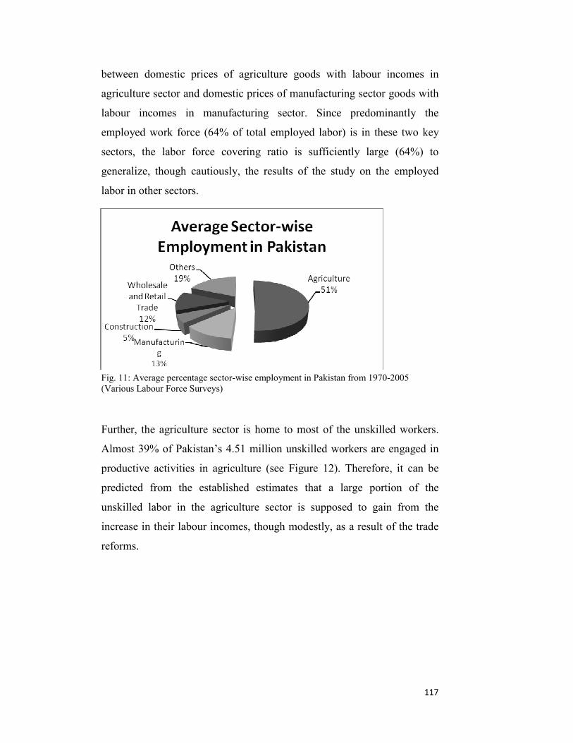
between domestic prices of agriculture goods with labour incomes in

agriculture sector and domestic prices of manufacturing sector goods with

labour incomes in manufacturing sector. Since predominantly the

employed work force (64% of total employed labor) is in these two key

sectors, the labor force covering ratio is sufficiently large (64%) to

generalize, though cautiously, the results of the study on the employed

labor in other sectors.

005

Fig. 11: Average percentage sector-wise employment in Pakistan from 1970-2

117

(Various Labour Force Surveys)

Further, the agriculture sector is home to most of the unskilled workers.

Almost 39% of Pakistan’s 4.51 million unskilled workers are engaged in

productive activities in agriculture (see Figure 12). Therefore, it can be

predicted from the established estimates that a large portion of the

unskilled labor in the agriculture sector is supposed to gain from the

increase in their labour incomes, though modestly, as a result of the trade

reforms.

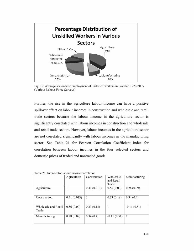
118

Fig. 12: Average sector-wise employment of unskilled workers in Pakistan 1970-2005 (Various Labour Force Surveys)

Further, the rise in the agriculture labour income can have a positive

spillover effect on labour incomes in construction and wholesale and retail

trade sectors because the labour income in the agriculture sector is

significantly correlated with labour incomes in construction and wholesale

and retail trade sectors. However, labour incomes in the agriculture sector

are not correlated significantly with labour incomes in the manufacturing

sector. See Table 21 for Pearson Correlation Coefficient Index for

correlation between labour incomes in the four selected sectors and

domestic prices of traded and nontraded goods.

Table 21: Inter-sector labour income correlation Agriculture Construction Wholesale

and Retail Trade

Manufacturing

Agriculture 1 0.41 (0.013) 0.56 (0.00) 0.28 (0.09)

Construction 0.41 (0.013) 1 0.23 (0.18) 0.34 (0.4)

Wholesale and Retail Trade

0.56 (0.00) 0.23 (0.18) 1 -0.11 (0.51)

Manufacturing 0.28 (0.09) 0.34 (0.4) -0.11 (0.51) 1

119

The values of the correlation coefficient in Table 21 predict a significant

linear correlation of labour incomes in agriculture and those in

construction and wholesale and retail trade. However, the labour incomes

in manufacturing do not show any significant linear correlation with

labour incomes in agriculture. The relatively large magnitudes of the

correlation coefficient (0.41 for correlation between labour incomes in

agriculture and construction and 0.56 for correlation between labour

incomes in agriculture and wholesale and retail trade) also indicate the

occurrence of a fairly strong correlation between labour incomes in

agriculture and the other two sectors.

5.6 Total (Price and Labour income) Effect on Household Welfare

The change in an ordinary household’s welfare is determined from the fact

that they are paying higher domestic prices of the consumer goods under

the protectionist policy and the net change in the labour incomes of

workers in the both agriculture and manufacturing sectors.

The net change in the ordinary household’s labour income due to the

proposed trade reforms (or due to the protectionist trade policy) can be

calculated as follows:

agri Manu∆LI x (No. of agriculture households)+∆LI (No. of manufacturing households)net∆LI=

Total no.of households in Agriculture and manufacturing(45)

From equation 45, the net change in the household’s labour income ( ∆LI)

can be calculated by adding changes in the total labour incomes in

agriculture and manufacturing i.e. change in the average labour incomes in

the two sectors multiplied by the number of households in the respective

sectors divided by the total number of households in both sectors.

Following Table 22 presents the year-wise and the average total net

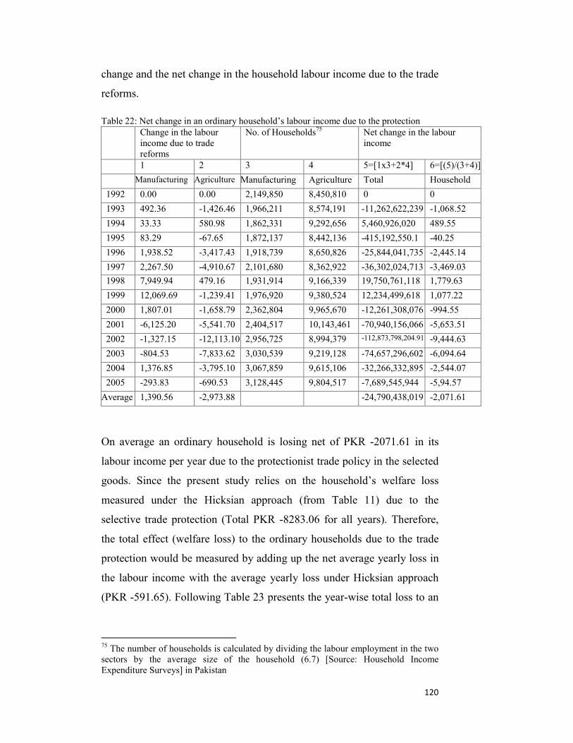
120

change and the net change in the household labour income due to the trade

reforms.

Table 22: Net change in an ordinary household’s labour income due to the protection Change in the labour

income due to trade reforms

No. of Households75 Net change in the labour income

1 2 3 4 5=[1x3+2*4] 6=[(5)/(3+4)]

Manufacturing Agriculture Manufacturing Agriculture Total Household

1992 0.00 0.00 2,149,850 8,450,810 0 0

1993 492.36 -1,426.46 1,966,211 8,574,191 -11,262,622,239 -1,068.52

1994 33.33 580.98 1,862,331 9,292,656 5,460,926,020 489.55

1995 83.29 -67.65 1,872,137 8,442,136 -415,192,550.1 -40.25

1996 1,938.52 -3,417.43 1,918,739 8,650,826 -25,844,041,735 -2,445.14

1997 2,267.50 -4,910.67 2,101,680 8,362,922 -36,302,024,713 -3,469.03 1998 7,949.94 479.16 1,931,914 9,166,339 19,750,761,118 1,779.63

1999 12,069.69 -1,239.41 1,976,920 9,380,524 12,234,499,618 1,077.22

2000 1,807.01 -1,658.79 2,362,804 9,965,670 -12,261,308,076 -994.55

2001 -6,125.20 -5,541.70 2,404,517 10,143,461 -70,940,156,066 -5,653.51

2002 -1,327.15 -12,113.10 2,956,725 8,994,379 -112,873,798,204.91 -9,444.63

2003 -804.53 -7,833.62 3,030,539 9,219,128 -74,657,296,602 -6,094.64

2004 1,376.85 -3,795.10 3,067,859 9,615,106 -32,266,332,895 -2,544.07

2005 -293.83 -690.53 3,128,445 9,804,517 -7,689,545,944 -5,94.57

Average 1,390.56 -2,973.88 -24,790,438,019 -2,071.61

On average an ordinary household is losing net of PKR -2071.61 in its

labour income per year due to the protectionist trade policy in the selected

goods. Since the present study relies on the household’s welfare loss

measured under the Hicksian approach (from Table 11) due to the

selective trade protection (Total PKR -8283.06 for all years). Therefore,

the total effect (welfare loss) to the ordinary households due to the trade

protection would be measured by adding up the net average yearly loss in

the labour income with the average yearly loss under Hicksian approach

(PKR -591.65). Following Table 23 presents the year-wise total loss to an

75 The number of households is calculated by dividing the labour employment in the two sectors by the average size of the household (6.7) [Source: Household Income Expenditure Surveys] in Pakistan

121

ordinary household owing to the selective protectionist policy against the

general relatively liberalizing economy.

Table 23: Total yearly loss to an ordinary Pakistani household due to the selective protectionist policy

HCV loss in an ordinary Household’s welfare

Net change in an ordinary household’s labour income

Total loss to an ordinary household due to the protection

Table 22: Column: 6 Net change in LI+ HCV welfare loss

PKR

1992 0.00 0 -0.001 1993 -42.32 -1,068.52 -1,110.84 1994 34.46 489.55 524.01 1995 -8.28 -40.25 -48.54 1996 -100.30 -2,445.14 -2,545.44 1997 -424.53 -3,469.03 -3,893.56 1998 -5839.60 1,779.63 -4,059.97 1999 -437.22 1,077.22 639.99 2000 -492.59 -994.55 -1,487.14 2001 -180.01 -5,653.51 -5,833.52 2002 -341.36 -9,444.63 -9,785.99 2003 -783.73 -6,094.64 -6,878.37 2004 189.42 -2,544.07 -2,354.65 2005 143.00 -594.57 -451.57 Average -591.65 -2,071.61 -2,663.26

According to the Table 23 the average annual loss to an ordinary Pakistani

household due to the trade protection in the selected goods against the

relatively liberalizing economy is equal to the PKR -2663.25.

The calculation of the trade-reform induced income changes of the poorest

households is rather difficult: Nearly forty percent of the unskilled

workers are working in agriculture. But as not all unskilled workers are

poor and not all poor are unskilled the attribution of changes of

agricultural income to the group of the poor remains somewhat vague. The

following Table 24 nevertheless calculates the total welfare effect (income

122

change plus change in MCS) for a group of households that are perceived

to represent the rural poor.

Table 24: Total welfare loss to the poorest Pakistani household due to the protectionist policy Yearly welfare loss

to the poorest household

Loss in the agriculture labour income

Yearly loss of protection to a single poorest household

MCS agri∆LI agri∆LI + welfare loss in MCS to the poorest household

Year PKR

1992 0.000 0.00 0.000

1993 -72.41 -1,426.46 -1,498.87

1994 47.18 580.98 628.16

1995 -7.68 -67.65 -75.33

1996 -136.44 -3,417.43 -3,553.87

1997 -278.81 -4,910.67 -5,189.48

1998 -329.21 479.16 149.95

1999 -970.94 -1,239.41 -2,210.35

2000 -1,374.56 -1,658.79 -3,033.35

2001 -2,756.56 -5,541.70 -8,298.26

2002 -2,817.58 -12,113.10 -14,930.68

2003 -2,954.22 -7,833.62 -10,787.84

2004 -3,421.42 -3,795.10 -7,216.52

2005 -2,162.53 -690.53 -2,853.06

Average -1,231.09 -2,973.88 -4,204.97

The results predict on average an even larger loss in the welfare of the

poorest household in Pakistan due to the protectionist policy. In an

average year they suffer a loss of PKR -4204.97 (compare it with loss of

PKR -2663.25 to an ordinary Pakistani household). This is because most

of the poorest households (39%) cluster in the rural areas and supply

unskilled labour in the agriculture sector which is hurt more due to the

protection. An ordinary Pakistani household seems to gain in the

manufacturing labour income however the poorest household does not

share in this gain. According to the SS theory, the relatively labour

oriented sector of the developing country gains from trade liberalization

and capital oriented sector loses. The reverse would be true in case of the

123

trade protectionist policy. The relatively labour oriented sector loses more

that the capital oriented sector gains. Further, the loss to the workers (in

terms of fall in the labour income) in agriculture sector (PKR -2973.88) is

larger than the gain (PKR 1390.56) in the labour income of the

manufacturing sector.

124

5.7 Discussion on the Statistical Results

The domestic prices of all selected traded goods are expected to fall by an

average of 65.31% when calculated at the falling general tariff instead of

the escalating actual tariff. The estimated domestic price of electricity

(nontraded good) is predicted to rise by 0.0043% and that of firewood to

fall by 0.043%. The predicted fall in the domestic prices of the selected goods

tends to change the consumption patterns and the utility of the ordinary and the

poorest households in Pakistan. Estimated demand equations for the average

households reveal patterns of household consumption in Pakistan. Four

goods out of 24 selected traded and nontraded goods have deviated from

the conventional demand theory. These goods—namely sugar, chilies,

beef, and fish—show a positive relationship between their domestic prices

and their quantities demanded. This may be explained as a result of

external shifts in the demand curves owing to the factors such as bumper

crop in agriculture due to better weather conditions or some other shocks.

The other traded and nontraded goods confirm the negative price-demand

relationship.

The estimated Marshallian demands (in linear and natural log-linear

forms) show a rise in the demand quantities due to a fall in the domestic

prices except in wheat, chilies, pulses, apple, potatoes, other vegetables,

sugar, firewood and electricity. The unexpected reaction in the demanded

quantities of these goods is the result of substitution and income effects of

the price change. In case of wheat, chilies, firewood and apples their

demands have reacted to the prices of their substitutes such as rice, other

spices, coal and kerosene and banana for each good respectively. The

households have partially substituted the demand for these goods with

their cheaper substitutes. Pulses demand equation assumes a negative

income effect hence as the domestic price of pulses falls, the negative

income effect dominates the total price effect. The demand for potatoes

125

has partially been diverted to its substitutable good onions. Further, the

fall in its complementary good’s (other vegetables) demand has caused

decrease in its demand. The price of sugar in its demand equation is

positive thus expectedly its demand has fallen as its price falls. Trade

reforms initiated higher price for electricity which caused a fall in its

demand. Since cigarettes’ estimated demand turns to be negative, it is

treated as zero. Since the study is measuring the losses in the household

welfare due to the protectionist trade policy, the rise in the quantity

demanded of the goods would be treated as the loss in the demand

quantities owing to the absence of the trade reforms.

Trade protection resulted in higher domestic prices of the selected traded

and nontraded goods (except electricity) and made households revise their

consumption patterns. The new household expenditures resulted in a

different level of household welfare. The loss in the households’ welfare

due to protection against the relatively liberalizing general economy is

measured by MCS and HCV. The loss in the household welfare, measured

using both approaches, reveals the loss of the ordinary Pakistani

households as a result of the selective trade protection. Methodologically,

MCS overestimates the change in the household welfare. HCV has been

used to correct the overestimation of the loss in MCS. Yet both

approaches strengthen the notion that households in Pakistan have

suffered profound losses in their welfare from the selective protectionist

policy. The average annual estimated welfare loss to an ordinary Pakistani

household under MCS is PKR -655.65 per year. The estimated annual

welfare loss to an ordinary Pakistani household in HCV has corrected the

Marshallian overestimated welfare loss and predicted an annual welfare

loss of PKR -591.65 to an ordinary Pakistani household. The discrepancy

between average figure of the total welfare loss under MCS and HCV is

around 9.76% which is more than the upper limit of 5% suggested by

Willig (1973) to approximate MCS with HCV. Further, the large

differences between Hicksian and Marshallian welfare losses in case of

126

onion (99337.315%), gas (2573.169%) and kerosene (1230.442%) defy

the upper bound proposed in Willig (1973) in case of only one price and

small income changes. Therefore the proposal of Willig (1973) is not

accepted here and relied on the HCV measure of the welfare.

Trade reforms also seem to affect the household income by influencing the

labour incomes in agriculture and manufacturing. The regressions in the

natural log linear form established the link between agriculture goods’

prices and agriculture labour incomes and between manufactured goods’

prices and manufacturing labour incomes. The estimated results indicate

that the selective protectionist policy has left the agriculture workers

worse off leaving them with an annual average loss of PKR -2937.88 in

their labour income and better off the manufacturing workers rewarding

them with an average annual gain of PKR 1390.56. This is perfectly in

line with the theoretical findings of S-S model which suggests that the

relatively labour oriented sectors gain and the relatively capital oriented

sectors lose as a result of the trade reforms in a developing country setting

and vice versa in case of protection. Manufacturing being relatively capital

oriented has gained and agriculture being the labour oriented has lost from

the trade protection in Pakistan.

The average labor statistics of the country reveal that more than 81% of

the total work force of the country and more than 73.58% of the total

unskilled labor force is clustering in three important sectors, namely

agriculture, construction, and wholesale and retail trade. The loss in

agriculture labour incomes due to protectionist policy is an omen that the

loss in agriculture would not only result in fall in the labour incomes for

agriculture workers but also workers from the other two sectors would

suffer from the labour income fall. Since unskilled workers are

approximated mostly as the poor in the country, so the loss in the labour

incomes of agriculture (unskilled) workers would be treated as a loss to

the poorest households.

127

Thus the loss to an ordinary Pakistani household due to the trade

protection is the sum of the two effects: loss in the labour income (net of

the loss in agriculture and gain in manufacturing) and loss in the HCV.

The average net loss per year in the labour income of the household is

PKR -2071.61. Hence the total loss to an ordinary household in Pakistan

owing to the trade protection is PKR -2663.25 [net annual average loss in

the household’s labour income (-2071.61) plus annual average welfare

loss in HCV (PKR -591.65)].

Unlike the estimated demand for the ordinary households, the demand for

the poorest households has been calculated from the available data on their

budget shares allocated for the selected goods and the calculated domestic

prices of traded and estimated domestic prices of nontraded goods. On

average the change in the quantity demanded in case of all goods has been

positive except electricity because its domestic price increased due to trade

reforms. The predicted annual average loss (PKR-1231.09) to the poorest

households due to the trade protection has been larger than the loss in the

(HCV) welfare of the ordinary Pakistani household (PKR -591.65). Thus

the total loss in the welfare of the poorest household due to the protection

(PKR -4204.97) is the total sum of the loss in MCS (PKR -1231.09) and

the loss in the labour income in agriculture (PKR -2973.88) due to the

reason that the 39% of the total elementary workers supply their unskilled

labour in agriculture sector.

The predicted measure of the households’ welfare under Hicksian

approach reveals that the incidence of trade protection has a fairly strong

impact on the poorest households’ welfare than on the ordinary. The

impact on the households’ consumption patterns is more profound in the

case of consumer goods than it is on the labour incomes. The factors like

absence of the variety of the household items in the local markets and a

small number of sellers lead to the monopolistic behavior of local

producers in determination of domestic prices. In the absence of trade

128

reforms, households have no option but to buy goods at higher prices

produced either inefficiently at higher costs or subject to the local

producers’ monopolies. The impact of trade protection on ordinary

Pakistani households’ welfare is smaller than the impact on that of the

Pakistani poorest households. About 50% of the welfare loss to the poorest

households originates from the demand for wheat, milk and beef, three

most important food items. Approximately 22.58% of the total

expenditure of the poorest household is allocated to these three goods

[12.13% for wheat, 8.80% for milk and 1.65% for beef] see Appendix

A1.1. The fall in the domestic prices of these goods would definitely have

resulted in a substantial fiscal space for the poorest households. Secondly,

because the fall in the agriculture labour income is larger than the gain in

the manufacturing labour income and most of the poor inhabit the rural

areas of the country where they supply their unskilled labour in

agriculture. An ordinary Pakistani household seems to gain from a rise in

the manufacturing labour income which a poorest household does not

seem to share when a protectionist policy is implemented.

The loss in labour income of agriculture workers is large (PKR -2973.88)

in comparison to the welfare loss to the ordinary households in HCV

(PKR-591.65). This indicates that the protection in the selected goods

favors the feudal archetype in the agriculture sector which suppresses the

wages of agriculture workers. Large land holdings of these feudal lords

provide them financial and political leverage over their land, as well as

over their tenants. Mostly, the tenants toil for their landowners for nothing

in return because they already owe large sums of money to the landlords.

Thus the large labour income change in the agriculture may be a possible

result of the proposed trade reforms in the selected goods which tend to

initiate the possible slacken off the agriculture workers from the

exploitative nature of the feudal setup along with removing the bottlenecks

on their wages via market oriented competition. This can be an

129

investigative interest for other researchers to explore the relevant issues in

this regard.

5.8 Limitations of the Study

This study examines the welfare loss to the ordinary and the poorest

Pakistani households and a loss or gain in agriculture and manufacturing

labour incomes due to a selective protectionist policy against a relatively

liberalizing general economy using Partial Equilibrium approach

supported by the General Equilibrium Technique. In the course of

analysis, since the key objectives involve measurement of the micro

impact of trade protection at household level, the impact on macro

indicators such as economic growth, foreign direct investment, GDP or

GNP, and Government revenues are out of the focus of the study.

The first limitation of the study is related to the import tariff data which is

calculated from the commodity-group wise tariff revenue and the import

quantities (C.I.F) in tons. Though the data on import tariff on the selected

commodities is calculated, yet it is compared with the import tariff data

available for some commodities for some years from the WTO online data

set. Since the domestic prices calculated with the average calculated tariff

show symmetry with those calculated at real tariff available for some

quantities for some years, the calculated domestic prices are reliable and

consistent.

Second, though the overall models of estimated household demand

equations are significant at F-statistic at 0 p-value and are reliable with

large F-values and R2 values, yet majority parameters in the estimated

demand equations are not having significant t-values at p<1. This

limitation in the estimated log and log-linear demand equations has been

overlooked since the significance of student t-statistics is mandatory in

sample studies. It is the indicator of power of results estimated from one

130

sample to be generalized over other samples of the population. The

statistics used in the present study originate from the national data series

from Pakistan and no sample data is used. Therefore the overall reliability

of the household demand estimates is not affected.

Third, owing to the unavailability of the required data series on the

consumption of the selected traded and nontraded goods by the poorest

households in Pakistan, the poorest household demand equations are not

estimated; rather they are calculated from the available information on the

poorest households’ budget shares allocated for consumption of the

selected traded and nontraded goods, domestic prices (including tariff) and

the annual household incomes.

Fourth, the labour allocation in the production of each individual good is

not available. The labour allocation in the production of each good is

approximated with the percentage share of each good in the total

agriculture or manufacturing production. Though in this method, the

underlying assumption of equal marginal productivity of labour in the

production of each good may not be true. Nevertheless in absence of the

accurate data on labour allocation in the production of each good, this

method can produce results which are closer to the reality.

131

6 Summary and Policy Recommendations

The key motive of the present study was to estimate the monetary losses in

the welfare of the ordinary as well as the poorest households of Pakistan

due to selective protectionist policy against the relatively liberalizing trend

in the general economy. The existing literature on the evidence of a trade-

poverty link provides details of two main cases coupled with individual

case studies and cross-country analyses. The first case is mostly known as

the Latin American failure and the second case is known as the East Asian

success story with liberalized trade policy. Latin American countries

(namely, Costa Rica, Mexico, Chile, Colombia, Argentina, and Uruguay)

liberalized their trade policies in the 1980s and observed a rise in wage

inequality. The higher skill premiums after trade liberalization widened

the gap between skilled and unskilled wages and thus resulted in worsened

poverty figures. On the other hand the East Asian countries (Hong Kong,

the Republic of Korea, Singapore, and Taiwan) followed liberalized trade

policy during the 1960s and observed higher wages for unskilled workers,

which reduced the skilled-unskilled wage gap. The lower skill premiums

in the region resulted in improvement in the well being of the poorest

households. The conflict of the evidence from the two cases may not be

termed as failure and success of open trade policy; rather, it can be the

point of the time of globalizing for both regions that caused the disparity

in outcomes. East Asian nations integrated into the global trade sector

during the 1960s with a large unskilled labor force and benefitted from the

comparative cost advantage. However, Latin American countries opened

for trade during the 1980s, when many countries like China, India,

Pakistan, and Bangladesh had already penetrated the world market with

large numbers of unskilled workers. Latin American labor during the

1980s, though unskilled in comparison with the labor from the developed

world, could not qualify as unskilled in comparison to the new influx of

unskilled labor from other Asian countries. Consequently, their

132

comparative advantage was brushed away by these Asian countries.

Secondly, the East Asian early globalizers, now having the experience of

two decades in manufacturing and trading, had accumulated large stocks

of capital and began pursuing more capital. The rise in the East Asian

demand for capital gave a big push to the global demand for technology. It

bore its effects on the skill premium in Latin American countries, too.

Individual and cross-country case studies of different developing countries

have had diverse outcomes regarding the impact of trade openness on

poverty figures. For example Dollar and Kraay (2001) found no evidence

of a systematic relationship between changes in trade and changes in

inequality. Thus they opine that the poor gain equally proportionate

increase in their incomes as the average national income rises as a result of

trade liberalization.

The present study should be perceived as an attempt to further the string of

individual case studies investigating the link between poverty, household

welfare, and liberalized trade regimes. The study applied H-O and S-S

models to establish a link between trade liberalization and poverty in

Pakistan. H-O assumptions suggest that developing countries find a

comparative advantage in importing capital-intensive goods and exporting

labor-intensive goods. This is true since developing countries like Pakistan

are labor-abundant countries and acquire labor as a relatively cheap factor

of production and thus enjoy a low cost advantage in producing labor-

intensive goods. On the other hand, developed countries, having abundant

capital, find it advantageous to produce capital-intensive products at home

and import labor-intensive products from abroad. The theoretical settings

provided in S-S Model are used to establish association of liberalized trade

policy with poverty. S-S Model predicts expansion in the labor-intensive

export sectors of developing countries and contraction in the capital-

intensive importing sectors as a result of liberalized trade policy.

Consequently, the returns to the factors of production in the two sectors

133

change respectively. Expanding sectors reward their workers with higher

wages, and contracting sectors penalize their workers with layoffs and cuts

in salaries.

To empirically test the applicability and soundness of the theoretical

findings of the two models, the study developed a set of regressions

involving the estimations of changes in the domestic prices of nontraded

goods with respect to change in the calculated domestic prices of traded

goods, and changes in the households’ labour income as a result of

protectionist policy in the selected goods against the relatively liberalizing

general economy Finally, the loss in household welfare is estimated

resulting from the selective protectionist policy against the general

liberalizing trend in the domestic prices of the selected traded and

nontraded goods and the labour incomes in agriculture and manufacturing

sectors. Two welfare approaches have been applied to measure the

predicted change in the average and the poorest households’ welfare. MCS

predicted loss in the welfare of the ordinary households as a result of

protection using Marshallian estimated demand quantities. The

protectionist policy in the selected goods led to the consumption of

different bundles of consumer goods, and different levels of the

households’ utility levels. As the Marshallian approach includes the

income effect in the total effect of a price change along with the

substitution effect while predicting household welfare, the estimates seem

to be overestimated. HCV approach adjusts the welfare estimates

downward to have an idea of accurate measure of loss in household

welfare caused by the substitution effect only. The Hicksian approach

anticipated a relatively smaller loss per year in household welfare (PKR -

591.65) than the Marshallian approach (PKR -655.65), the core outcome

of the study that the protectionist trade policy hurts the households

remains unaffected in both approaches. Given that the objective of the

study is to measure the price effects of the protectionist trade policy in

selected goods against the relatively liberalized general trend in the

134

economy, the Hicksian approach is relied upon as an accurate measure of

households’ welfare since it excludes the income effect from the price

effect.

Further, the impact of selective trade protection on the welfare of the

poorest households is estimated separately. The demands of the poorest

households are calculated from the available data on the budget shares

allocated to the consumer goods and their estimated domestic prices. The

poorest households’ demands for the selected goods are then employed to

measure the change in the poorest households’ MCS. Due to the lack of

appropriate data on the poorest households’ consumption, the poorest

households’ demands are not estimated but calculated from their budget

shares allocated for the selected goods.

According to the estimations under both welfare approaches, an ordinary

household loses profoundly due to the protection in the selected goods

against the relatively liberalizing trend in the economy in general. The

poorest household loses more (PKR -4204.97) than the loss to an ordinary

Pakistani household (PKR -2663.255) because the protection hurts

agriculture sector more severely than the other sectors amid rewarding the

relatively capital oriented manufacturing sector.

Due to unavailability of the data on goods from other sectors, the

regressions on the labour income-price link involve only the agriculture

and manufacturing. The empirical results on the association between

labour incomes in agriculture and manufacturing and the domestic prices

of selected traded and nontraded goods predict a fall in agriculture labour

income (PKR- 2973.88) and gain (PKR 1390.56) in the manufacturing

labour income owing to the selective protection. The net loss in the

ordinary Pakistani household’s labour income is thus PKR -2071.61.

Given that more than 81% of the total work force is clustering in three

important sectors—namely agriculture, construction, and wholesale and

retail trade—and there is a positive and statistically significant correlation

135

of labour income in agriculture with labour incomes in construction and

wholesale and retail trade, the predicted labour income effect does not

seem to be limited to agriculture workers alone. The workers from the

other two sectors are likely to suffer the loss due to the selective

protection. Further, the average percentage of unskilled workers in the

three sectors (excluding manufacturing) is 73.58%, which is a significant

portion of the total number of unskilled workers in the country. Since

unskilled workers are approximated mostly as the poor in the country, so

the loss in the labour incomes of (agriculture) unskilled workers may be

treated as a loss in the labour income of the poorest households.

Summarizing the whole cascade of empirical evidence and estimated

predictions, it can be asserted that a liberal trade policy is set to bring

improvements in the welfare of an ordinary and the poorest household in

Pakistan, with the welfare loss to the poorest household seemingly larger

than to an ordinary household because the poorest households cluster in

agriculture and the sector is hurt severely under trade protection.

Therefore, more open trade policy can be recommended to policy makers

in Pakistan as a development and households’ welfare tool. Poverty in the

country can be controlled, and the household welfare can be boosted by

following an export-oriented policy similar to that of East Asian countries.

Trade protection even in the selected goods hurts the poorest households

and distorts the domestic prices of household consumption goods. Further,

to ensure that the benefits of trade reforms reach the agriculture workers,

land reforms and the competitive market principles can be initiated and

implemented in the agriculture sector. The country’s feudal structure,

particularly in the agriculture sector, seems to be the biggest impediment

to the benefits of trade reforms reaching down to agricultural workers.

136

Bibliography Agenore, P. (2002) “Does Globalization Hurt Poor?” Policy Research

Working Paper No. 2922, World Bank Institute, Poverty Reduction and

Economic Management Division, October.

Ahmed, J.; (2001) “Causality between Exports and Economic Growth:

What do the Econometrics Studies Tell Us?” Pacific Economic Review,

1(6), 147-167.

Appleton, S. (2001) “Poverty Reduction during Growth: The Case of

Uganda, 1992-2000.” Unpublished manuscript, University of Nottingham.

Appleyard, D. R.; Field, A. J. Jr. and Cobb. S. L. (2006) International

Economics 5th edition McGraw–Hill Irwin.

Attanasio, O.; Goldberg, P. K. and Pavcnik, N. (2004), “Trade Reforms

and Wage Inequality in Columbia”, Journal of Development Economics,

74, 331-334.

Beyer, H, and Vergara, R. (1999) “Productivity and Economic Growth: The

Case of Chile”, Central Bank of Chile.

Black, Fischer (1996) Exploring General Equilibrium Cambridge

Massachusetts: The MIT Press Vol. 5, Issue 3, 335-338.

Bleaney, M. (1993) “Liberalization and the Terms of Trade of Developing

Countries: A Cause for Concern?” The World Economy, Vol. 16, Issue 4,

453-466.

Borges, A. M. (1986) “Applied General Equilibrium Models: An

Assessment of Their Usefulness for Policy Analysis”, OECD Economic

Studies No. 7, autumn, 19.

137

Carvajal, A. (2006) “Lecture Notes on General Equilibrium Theory”, Royal

Holloway College, University of London.

Case, K. E. and Fair, R. C. (1999) Principles of Economics 5th edition,

Prentice-Hall.

Chaudhuri, S. and Ghosh, A. (2001); “Trade Liberalization and Increasing

Wage Inequality in Latin America: Existing Explanations Challenged by

Theories”, Dept. of Economics, University of Calcutta Working Paper

Series.

Cockburn, J. (2001), “Trade Liberalization and Poverty in Nepal: A

Computable General Equilibrium Microsimulation Approach”, CREFA

Working Paper 11, 01-18.

Cogneau, D. and Robilliard, A. S. (2000) “Growth, Distribution and Poverty

in Madagascar: Learning from a Microsimulation Model in a General

Equilibrium Framework” IFPRI TMD Discussion Paper 61.

Coxhead, Ian. A. and War, P.G. (1995) “Does Technical Progress in

Agriculture Alleviate Poverty? A Philippines Case Study” Australian

Journal of Agriculture Economics, 39(1), 25-54.

Deaton, A. (1989) “Rice Price and Income Distribution in Thailand: A

Nonparametric Analysis”, Economic Journal 99, 1-37.

Dercon, S. (2001) “The Impact of Economic Reforms on Households in

Rural Ethiopia 1989-1995.” Centre for the Study of African Economies,

Dept. of Economics and Jesus College, Oxford University.

Dixit, A. and Norman, V. (1980) Theory of International Trade: A Dual,

General Equilibrium Approach, Cambridge Economic Handbooks.

Dollar, D. and Kraay, A. (2001) “Trade, Growth, and Poverty”

Development Research Group, The World Bank.

138

Edwards, S. (1993) “Openness, Trade Liberalization and Growth in

Developing Countries, Journal of Economic Literature, 3(31), 1358-1393.

Esfahani, H. S. (1991) “Exports, Imports and Economic Growth in Semi-

industrial Countries” Journal of Development Economics, 35, 93-1 16.

Evans, D. (2001) “Identifying Winners and Losers in Southern Africa from

Global Trade Policy Reform: Integrating Findings from GTAP and Poverty

Case Studies for a Zambian Example” Paper prepared for the ESRC

Development Economics/International Economics Conference, Nottingham

University, April 5-7.

Federal Board of Revenue, Pakistan online dataset Portal

Federal Bureau of Statistics (1998), 50 years of Pakistan in Statistics, Vol. I-

IV (1947-1997).

Feenstra, R. C. and Hanson, G. H. (1997) “Foreign Direct Investment and

Relative Wages: Evidence from Mexico's Maquiladoras", Journal of

International Economics, 42: 371-394.

Fields, G. (1994) “Changing Labor Market Conditions and Economic

Development in Hong Kong, the Republic of Korea, Singapore, and Taiwan,

China” The World Bank Economic Review 8(3): 395-414.

Fofack, H.; Célestin, M.; and Tuluy, H. (2001) “Household Welfare and

Poverty Dynamics in Burkina Faso: Empirical Evidence from Household

Surveys.” World Bank Policy Research Paper 2590.

Frankel, A. J. and Romer, D. (1999) “Does Trade Cause Growth?”

American Economic Review, 3(89), 379-389.

Gujarati, D. N. (2004) Basic Econometrics, 4th Edition, The McGraw Hill

Company.

139

Harding, A. (2007) “Challenges and Opportunities of Dynamic

Microsimulation Modeling” presented in General Conference of

Microsimulation Association, Vienna, August.

Harrison, A. and McMillan, M. (2007) “On the Links between Globalization

and Poverty”, Journal Economic Inequality 1(5):123-134.

Hanson. G. H and Harrison A.; (1999) “Trade Liberalization and Wage

Inequality in Mexico” Industrial and Labour Relations Review, Vol. 52,

No.2.

Harrison, G. W.; Rutherford, T. F. and Tarr, D. G. (2001) “Trade

Liberalization, Poverty and Efficient Equity” Journal of Development

Economics 71, 97-128.

Hausman, Jerry A. (1981), “Exact Consumer’s Surplus and Dead Weight

Loss”, American Economic Review, 71 (4), 662–76.

Hicks, J. R. (1939); “The Foundations of Welfare Economics”, Economic

Journal, 49 (196), 696–712.

Ianchovichina, E.; Nicita, A. and Soloaga, I. (2001) “Trade Reform and

Household Welfare: The Case of Mexico” The World Bank Policy Research

Working Paper 2667 August.

International Labour Organization online datasets

Jones, R. W. (1965) “The Structure of Simple General Equilibrium Models”

The Journal of Political Economy, 6 (73), 557-572.

Just, R.E.; Hueth, D.L.; Schmitz, A.(2004) The Welfare Economics of

Public Policy: A Practical Approach to Project and Policy Evaluation

Edward Elgar Publishing Limited, USA.

140

Kaplinsky, R. (1993) “Export Processing Zones in the Dominican Republic:

Transforming Manufactures into Commodities” World Development

21(ll):1851-65.

Keunne, R. E. (1963) The Theory of General Economic Equilibrium,

Princeton University Press, Princeton, New Jersey.

Kemal, A. R.; Siddiqui, R. and Kemal, M. A. (2002) “An Assessment of the

Impact of Trade Liberalization on Welfare in Pakistan: A General

Equilibrium Analysis”, MIMAP Technical Paper Series No. 16, PIDE

Islamabad.

Khan, A. H. (1998) “The Experience of Trade Liberalization in Pakistan”,

Pakistan Development Review, 37:4 Part II, 37:4, 661-685.

Kim, K. S., and Vorasopontaviporn, P. (1989) “Foreign Trade and the

Distribution of Income in Thailand” Working Paper 124, Helen Kellogg

Institute for International Studies, University of Notre Dame, Notre Dame.

Krueger, A. O. (1983) Trade and Employment in Developing Countries, 3:

Synthesis and Conclusions (pp. 30 – 54), University of Chicago Press.

Krueger, A. O. (1990) “Asian Trade and Growth Lessons”, The American Economic Review (AER), 80(2), 108 - 12.

Kuenne, R. E (1963) The Theory of General Equilibrium Princeton, NJ Princeton University Press.

Leamer, E. E. (1995) “The Heckscher-Ohlin Model in Theory and Practice,

Princeton Studies in International Finance, No. 77.

Levinsohn J.; Berry, S. and Friedman, J. (1999) “Impacts of the Indonesian

Economic Crisis: Price Changes and the Poor”, NBER Working Paper 7194.

Levy, S. and Sweder van W. (1992), "Maize and the Free Trade Agreement

between Mexico and the United States", The World Bank Economic

Review, Vol6, 3:481-502.

141

Lloyd, J. P. and Zhang, X. G. (2006) “The Armington Model” Australian

Government Productivity Commission Staff Working Paper.

Loefgren, H. (1999) “Trade Reforms and Poor in Morocco: A Rural-Urban

General Equilibrium Analysis of Reduced Protection” IFPRI TMD

Discussion Paper 38.

McCulloch, N. and Calandrino, M. (2001) “Poverty Dynamics in Rural

Sichuan between 1991 and 1995.” Paper prepared for the ESRC

Development Economics/International Economics Conference,

Nottingham University, April 5-7, 2001.

Malik, S. J. (2005) “Agricultural Growth and Rural Poverty: A Review of

the Evidence” ADB Pakistan Resident Mission Working Paper No. 2.

Mandal, R.K.; (2007), Microeconomics: Theory and Applications, Atlantic

Publishers and Distributors, India.

Mas-Colell, A.; Whinston, M. and Green, J. (1995) Microeconomic Theory,

Oxford University Press.

Merz, J. (1995) “MICSIM: Concept, Developments and Applications of a

PC-Microsimulation Model for Research and Teaching” MPRA Paper No.

16029.

Minot, N. and Blauch, B. (2002) “Poverty Mapping with Aggregate Census

Data: What is the Loss in Precision?” Review of Development Economics,

9(1), 5-24.

Orcutt, G. H. (1957) “A New Type of Socio-Economic System” The

Review of Economics and Statistics, 39, 116 - 123.

Porto, G. G. (2003) “Trade Reforms, Market Access and Poverty in

Argentina” World Bank Policy Research Working Paper No. 3135.

142

Porto, G. G. (2006) “Using Survey Data to Assess the Distributional Effects

of Trade Policy” Journal of International Economics 70, 140-160.

Ravallion, M. (2004) “Looking Beyond Averages in the Trade and Poverty

Debate” World Bank Policy Research Working Paper 3461.

Ravallion, M. and Whalley, V. D (1991) “Impact of Poverty on Food

Pricing Reforms: A Welfare Analysis of Indonesia, Journal of Policy

Modeling 13(2):281-299.

Reimer, J. J. (2002) “Estimating the Poverty Impacts of Trade

Liberalization, World Bank Policy Research Working Paper No. 2922.

Robbins, D. J. and Gindling, T. H. (1999) “Trade Liberalization and

Relative Wages for More Skilled Workers in Costa Rica, The Review of

Development Economics, 3(2), 140-154.

Robbins, D. J. (1994a) “Malaysian Wage Structure and Its Causes” Harvard

Institute for International Development, Cambridge, Mass.

Robbins, D. J. (1994) “Worsening Relative Wage Dispersion in Chile during

Trade Liberalization, and Its Causes: Is Supply at Fault?” Harvard Institute

of Development, Development Discussion Paper Series No. 484, 50.

Robbins, D. J. (1996) “Evidence on Trade and Wages in the Developing

World” OECD Development Centre, Working Paper No. 119, (96) 182.

Robbins, D. J. and Zveglich, J. (1995a) “Skill-Bias in Recent Taiwanese

Growth” Harvard Institute for International Development Cambridge, Mass.

Robilliard, A. S.; Bourguignon, F. and Robinson, S. (2001) “Crisis and

Income Distribution: A Micro-Macro Model for Indonesia”, Draft for

Preliminary Results, June.

143

Rodriguez, F. and Rodrik, D. (1999) “Trade Policy and Economic Growth:

A Skeptic's Guide to the Cross-National Evidence” University of Maryland

and Harvard University, (Revised May).

Sachs, J. D.; Warner, A.; Anders, A. and Fischer, S. (1995) “Economic

Reforms and Process of Global Integration”, Brookings Papers on Economic

Activity, 1(1995), 1-118.

Sadoulet, E. and De Janvrry, A. (1992), “Agricultural Trade Liberalization

and Low Income Countries: A GE Multimarket Approach” American

Journal of Agriculture Economics 74 (2): 268-280.

Saggay, A.; Heshmati, A. and Adel Dhif, M. (2006) “Effects of Trade

Liberalization on Domestic Prices: Some Evidence from Tunisian

Manufacturing” The Ratio Working Paper 96.

Samuelson, P. A. (1953) “Prices of Factors and Goods in General

Equilibrium” The Review of Economic Studies, 1(21).

Shorrocks, A. F. (1982) “Inequality Decomposition by Factor Components”

Econometrica, 1(50), 193-212.

Siddiqui, R. and Kemal, A. R. (2002) “Remittances, Trade Liberalization,

and Poverty in Pakistan: The Role of Excluded Variables in Poverty Change

Analysis” The Pakistan Development Review 3(45) 383-415.

Simpson, D. (1975) General Equilibrium Analysis: An Introduction XVIII,

Basil Blackwell, Oxford.

Slaughter, M. J. (2001) “Does Trade Liberalization Converge Factor Prices?

Evidence from the Antebellum Transportation Revolution”, Journal of

International Trade and Economic Development 3(10), 339–362.

Statistical Division (2003) “Household Integrated Expenditure Survey”

Ministry of Economic Affairs and Statistics, Federal Bureau of Statistics,

Government of Pakistan Round 4: 2001-02.

144

Smith, A. (1776) An Inquiry into the Nature and Causes of the Wealth of

Nations ISBN 0-87975-705-1.

Suranovic. S.; (2010) International Trade: Theory and Policy, The George

Washington University, Washington, D.C.

United States Agriculture Department online database

Varian, H. R. (2003), Intermediate Microeconomics - A Modern Approach

W.W. Norton Company New York.

Walras, L. (1874) Elements of Pure Economics Harvard University Press,

ISBN 978-0678060285

Whalley, J. (1974) “How Reliable is the Partial Equilibrium Analysis?” The

Review of Economics and Statistics, 3(57), 299-310.

Willig, R. D. (1973), Consumer’s Surplus: A Rigorous Cookbook,

Technical Report No. 98, Stanford, CA: Stanford University Press: Institute

for Mathematical Studies in the Social Sciences.

Willig. R. D. (1976), “Consumer’s Surplus without Apology” The American

Economic Review, 4(66), 589-597.

Winters, L. A. (2000) “Trade and Poverty: Is There a Connection?” Essay

prepared at the request of WTO. Based on research reported in two papers

presented as background studies to the World Bank's World Development

Report 2000/1 Winters (2000a, b).

Wood, A. (1995) “How Trade Hurt Unskilled Workers? Journal of

Economic Perspectives, Volume 9 No. 3, (summer), 57-80.

Wood, A. (1997) “Openness and Wage Inequality in Developing Countries:

The Latin American Challenge to East Asian Conventional Wisdom” The

World Bank Economic Review, 1(11).

145

Woodland, A. D. (1982) International Trade and Resource Allocation,

North-Holland, Amsterdam and New York, 1982.

World Bank (1989, 1990, 2002) Annual Reports

Yang, Y. Y. and Hwang, M. (1999) “Effects of Trade Liberalization on Domestic Prices: The Evidence from Korea 1983-1995” Department of Economics, California State University, Sacramento and Berkley (January).

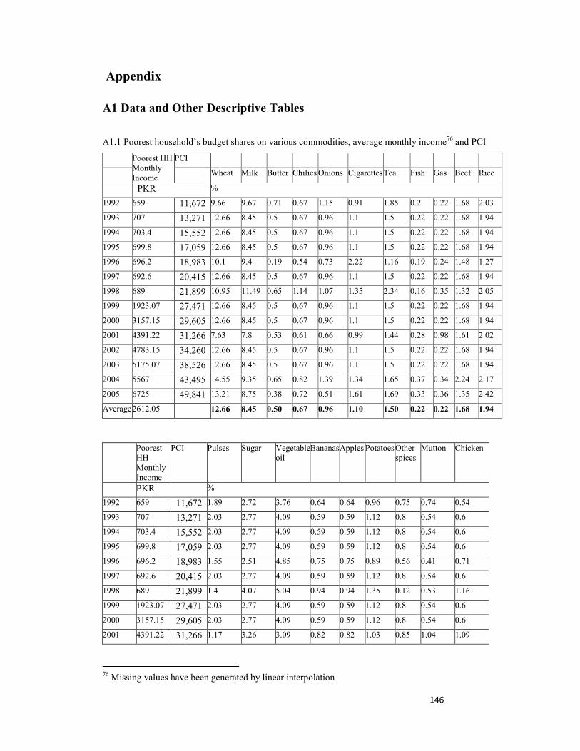
146

Appendix

A1 Data and Other Descriptive Tables

A1.1 Poorest household’s budget shares on various commodities, average monthly income76 and PCI

Poorest HH Monthly Income

PCI

Wheat Milk Butter Chilies Onions Cigarettes Tea Fish Gas Beef Rice

PKR %

1992 659 11,672 9.66 9.67 0.71 0.67 1.15 0.91 1.85 0.2 0.22 1.68 2.03

1993 707 13,271 12.66 8.45 0.5 0.67 0.96 1.1 1.5 0.22 0.22 1.68 1.94

1994 703.4 15,552 12.66 8.45 0.5 0.67 0.96 1.1 1.5 0.22 0.22 1.68 1.94

1995 699.8 17,059 12.66 8.45 0.5 0.67 0.96 1.1 1.5 0.22 0.22 1.68 1.94

1996 696.2 18,983 10.1 9.4 0.19 0.54 0.73 2.22 1.16 0.19 0.24 1.48 1.27

1997 692.6 20,415 12.66 8.45 0.5 0.67 0.96 1.1 1.5 0.22 0.22 1.68 1.94

1998 689 21,899 10.95 11.49 0.65 1.14 1.07 1.35 2.34 0.16 0.35 1.32 2.05

1999 1923.07 27,471 12.66 8.45 0.5 0.67 0.96 1.1 1.5 0.22 0.22 1.68 1.94

2000 3157.15 29,605 12.66 8.45 0.5 0.67 0.96 1.1 1.5 0.22 0.22 1.68 1.94

2001 4391.22 31,266 7.63 7.8 0.53 0.61 0.66 0.99 1.44 0.28 0.98 1.61 2.02

2002 4783.15 34,260 12.66 8.45 0.5 0.67 0.96 1.1 1.5 0.22 0.22 1.68 1.94

2003 5175.07 38,526 12.66 8.45 0.5 0.67 0.96 1.1 1.5 0.22 0.22 1.68 1.94

2004 5567 43,495 14.55 9.35 0.65 0.82 1.39 1.34 1.65 0.37 0.34 2.24 2.17

2005 6725 49,841 13.21 8.75 0.38 0.72 0.51 1.61 1.69 0.33 0.36 1.35 2.42

Average 2612.05 12.66 8.45 0.50 0.67 0.96 1.10 1.50 0.22 0.22 1.68 1.94

Poorest HH Monthly Income

PCI Pulses Sugar Vegetable oil

Bananas Apples Potatoes Other spices

Mutton Chicken

PKR %

1992 659 11,672 1.89 2.72 3.76 0.64 0.64 0.96 0.75 0.74 0.54

1993 707 13,271 2.03 2.77 4.09 0.59 0.59 1.12 0.8 0.54 0.6

1994 703.4 15,552 2.03 2.77 4.09 0.59 0.59 1.12 0.8 0.54 0.6

1995 699.8 17,059 2.03 2.77 4.09 0.59 0.59 1.12 0.8 0.54 0.6

1996 696.2 18,983 1.55 2.51 4.85 0.75 0.75 0.89 0.56 0.41 0.71

1997 692.6 20,415 2.03 2.77 4.09 0.59 0.59 1.12 0.8 0.54 0.6

1998 689 21,899 1.4 4.07 5.04 0.94 0.94 1.35 0.12 0.53 1.16

1999 1923.07 27,471 2.03 2.77 4.09 0.59 0.59 1.12 0.8 0.54 0.6

2000 3157.15 29,605 2.03 2.77 4.09 0.59 0.59 1.12 0.8 0.54 0.6

2001 4391.22 31,266 1.17 3.26 3.09 0.82 0.82 1.03 0.85 1.04 1.09

76 Missing values have been generated by linear interpolation

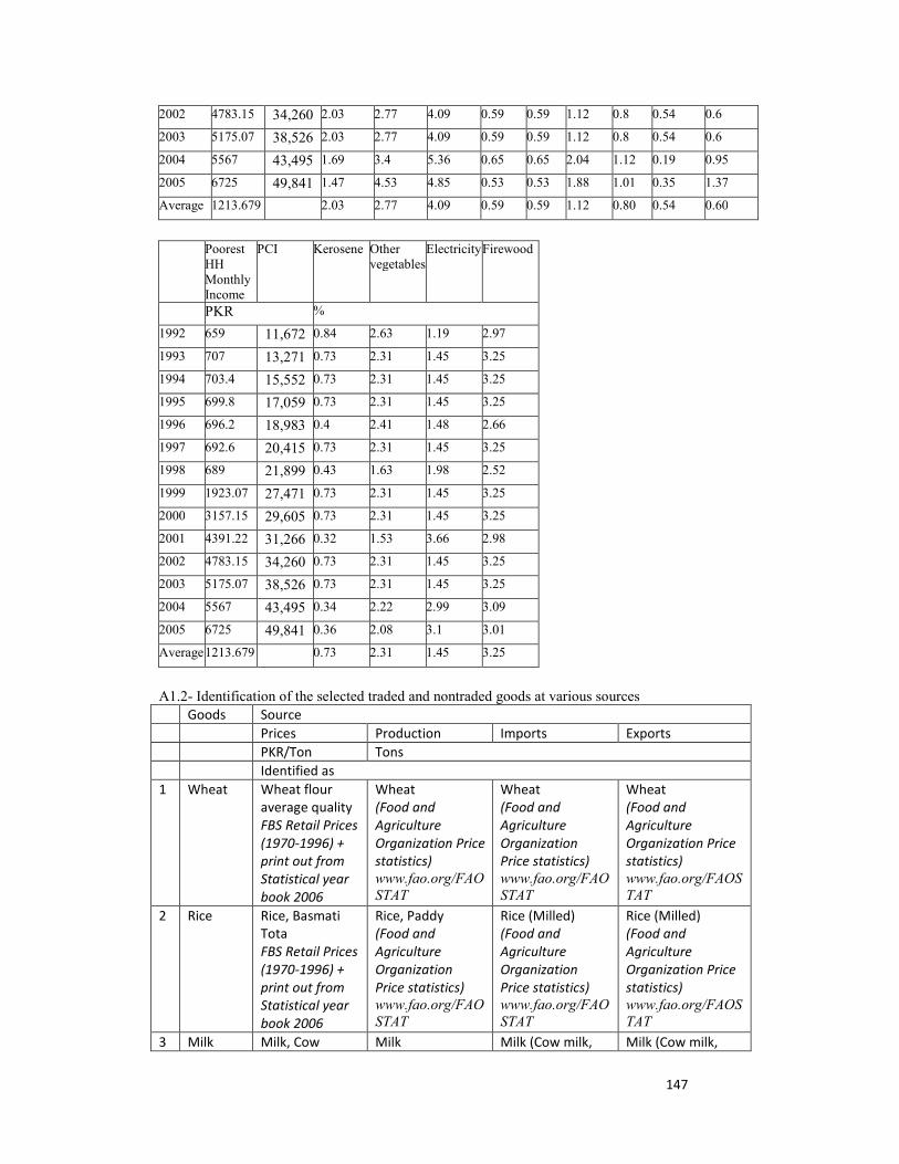
147

2002 4783.15 34,260 2.03 2.77 4.09 0.59 0.59 1.12 0.8 0.54 0.6

2003 5175.07 38,526 2.03 2.77 4.09 0.59 0.59 1.12 0.8 0.54 0.6

2004 5567 43,495 1.69 3.4 5.36 0.65 0.65 2.04 1.12 0.19 0.95

2005 6725 49,841 1.47 4.53 4.85 0.53 0.53 1.88 1.01 0.35 1.37

Average 1213.679 2.03 2.77 4.09 0.59 0.59 1.12 0.80 0.54 0.60

Poorest

HH Monthly Income

PCI Kerosene Other vegetables

Electricity Firewood

PKR %

1992 659 11,672 0.84 2.63 1.19 2.97

1993 707 13,271 0.73 2.31 1.45 3.25

1994 703.4 15,552 0.73 2.31 1.45 3.25

1995 699.8 17,059 0.73 2.31 1.45 3.25

1996 696.2 18,983 0.4 2.41 1.48 2.66

1997 692.6 20,415 0.73 2.31 1.45 3.25

1998 689 21,899 0.43 1.63 1.98 2.52

1999 1923.07 27,471 0.73 2.31 1.45 3.25

2000 3157.15 29,605 0.73 2.31 1.45 3.25

2001 4391.22 31,266 0.32 1.53 3.66 2.98

2002 4783.15 34,260 0.73 2.31 1.45 3.25

2003 5175.07 38,526 0.73 2.31 1.45 3.25

2004 5567 43,495 0.34 2.22 2.99 3.09

2005 6725 49,841 0.36 2.08 3.1 3.01

Average 1213.679 0.73 2.31 1.45 3.25

A1.2- Identification of the selected traded and nontraded goods at various sources Goods Source Prices Production Imports Exports PKR/Ton Tons Identified as 1 Wheat Wheat flour

average quality FBS Retail Prices (1970-1996) + print out from Statistical year book 2006

Wheat (Food and Agriculture Organization Price statistics) www.fao.org/FAOSTAT

Wheat (Food and Agriculture Organization Price statistics) www.fao.org/FAOSTAT

Wheat (Food and Agriculture Organization Price statistics) www.fao.org/FAOSTAT

2 Rice Rice, Basmati Tota FBS Retail Prices (1970-1996) + print out from Statistical year book 2006

Rice, Paddy (Food and Agriculture Organization Price statistics) www.fao.org/FAOSTAT

Rice (Milled) (Food and Agriculture Organization Price statistics) www.fao.org/FAOSTAT

Rice (Milled) (Food and Agriculture Organization Price statistics) www.fao.org/FAOSTAT

3 Milk Milk, Cow Milk Milk (Cow milk, Milk (Cow milk,

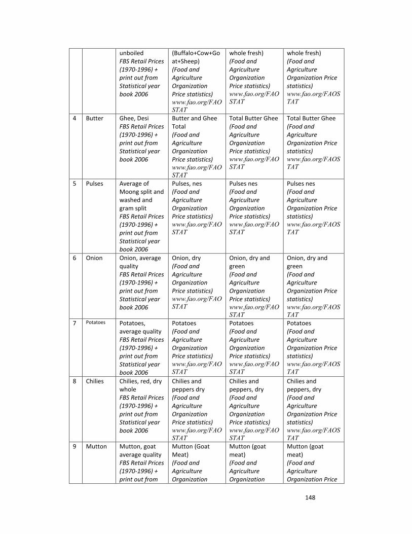
148

unboiled FBS Retail Prices (1970-1996) + print out from Statistical year book 2006

(Buffalo+Cow+Goat+Sheep) (Food and Agriculture Organization Price statistics) www.fao.org/FAOSTAT

whole fresh) (Food and Agriculture Organization Price statistics) www.fao.org/FAOSTAT

whole fresh) (Food and Agriculture Organization Price statistics) www.fao.org/FAOSTAT

4 Butter Ghee, Desi FBS Retail Prices (1970-1996) + print out from Statistical year book 2006

Butter and Ghee Total (Food and Agriculture Organization Price statistics) www.fao.org/FAOSTAT

Total Butter Ghee (Food and Agriculture Organization Price statistics) www.fao.org/FAOSTAT

Total Butter Ghee (Food and Agriculture Organization Price statistics) www.fao.org/FAOSTAT

5 Pulses Average of Moong split and washed and gram split FBS Retail Prices (1970-1996) + print out from Statistical year book 2006

Pulses, nes (Food and Agriculture Organization Price statistics) www.fao.org/FAOSTAT

Pulses nes (Food and Agriculture Organization Price statistics) www.fao.org/FAOSTAT

Pulses nes (Food and Agriculture Organization Price statistics) www.fao.org/FAOSTAT

6 Onion Onion, average quality FBS Retail Prices (1970-1996) + print out from Statistical year book 2006

Onion, dry (Food and Agriculture Organization Price statistics) www.fao.org/FAOSTAT

Onion, dry and green (Food and Agriculture Organization Price statistics) www.fao.org/FAOSTAT

Onion, dry and green (Food and Agriculture Organization Price statistics) www.fao.org/FAOSTAT

7 Potatoes Potatoes, average quality FBS Retail Prices (1970-1996) + print out from Statistical year book 2006

Potatoes (Food and Agriculture Organization Price statistics) www.fao.org/FAOSTAT

Potatoes (Food and Agriculture Organization Price statistics) www.fao.org/FAOSTAT

Potatoes (Food and Agriculture Organization Price statistics) www.fao.org/FAOSTAT

8 Chilies Chilies, red, dry whole FBS Retail Prices (1970-1996) + print out from Statistical year book 2006

Chilies and peppers dry (Food and Agriculture Organization Price statistics) www.fao.org/FAOSTAT

Chilies and peppers, dry (Food and Agriculture Organization Price statistics) www.fao.org/FAOSTAT

Chilies and peppers, dry (Food and Agriculture Organization Price statistics) www.fao.org/FAOSTAT

9 Mutton Mutton, goat average quality FBS Retail Prices (1970-1996) + print out from

Mutton (Goat Meat) (Food and Agriculture Organization

Mutton (goat meat) (Food and Agriculture Organization

Mutton (goat meat) (Food and Agriculture Organization Price

149

Statistical year book 2006

Price statistics) www.fao.org/FAOSTAT

Price statistics) www.fao.org/FAOSTAT

statistics) www.fao.org/FAOSTAT

10 Beef Beef, Cow, average quality FBS Retail Prices (1970-1996) + print out from Statistical year book 2006

Cattle +Buffalo meat (Food and Agriculture Organization Price statistics) www.fao.org/FAOSTAT

Cattle meat (no data available on Buffalo meat trade) (Food and Agriculture Organization Price statistics) www.fao.org/FAOSTAT

Cattle meat (no data available on Buffalo meat trade) (Food and Agriculture Organization Price statistics) www.fao.org/FAOSTAT

11 Fish Fish, Rahu FBS Retail Prices (1970-1996) + print out from Statistical year book 2006

Fish FBS Book 1970-1996+ print out from Statistical year book 2006 from 1996-2005

12 Tea Tea, Lipton yellow label/ Isphahani FBS Retail Prices (1970-1996) + print out from Statistical year book 2006

Tea FBS Book 1970-1996+ print out from Statistical year book 2006 from 1996-2005

Tea (Food and Agriculture Organization Price statistics) www.fao.org/FAOSTAT

Tea (Food and Agriculture Organization Price statistics) www.fao.org/FAOSTAT

13 Sugar Sugar, Refined FBS Retail Prices (1970-1996) + print out from Statistical year book 2006

Sugar FBS Book 1970-1996 manufactured products chapter+ print out from Statistical year book 2006 from 1996-2005

Sugar, Refined (Food and Agriculture Organization Price statistics) www.fao.org/FAOSTAT

Sugar, Refined (Food and Agriculture Organization Price statistics) www.fao.org/FAOSTAT

14 Vegetable Oil

Ghee, vegetable Dalda Tin FBS Retail Prices (1970-1996) + print out from Statistical year book 2006

Groundnut+Linseed+Rapeseed+Sesame+Soyabean+Sunflower oils (Food and Agriculture Organization Price statistics)

Oil of Vegetable origin nes (Food and Agriculture Organization Price statistics) www.fao.org/FAOSTAT

Oil of Vegetable origin nes (Food and Agriculture Organization Price statistics) www.fao.org/FAOSTAT

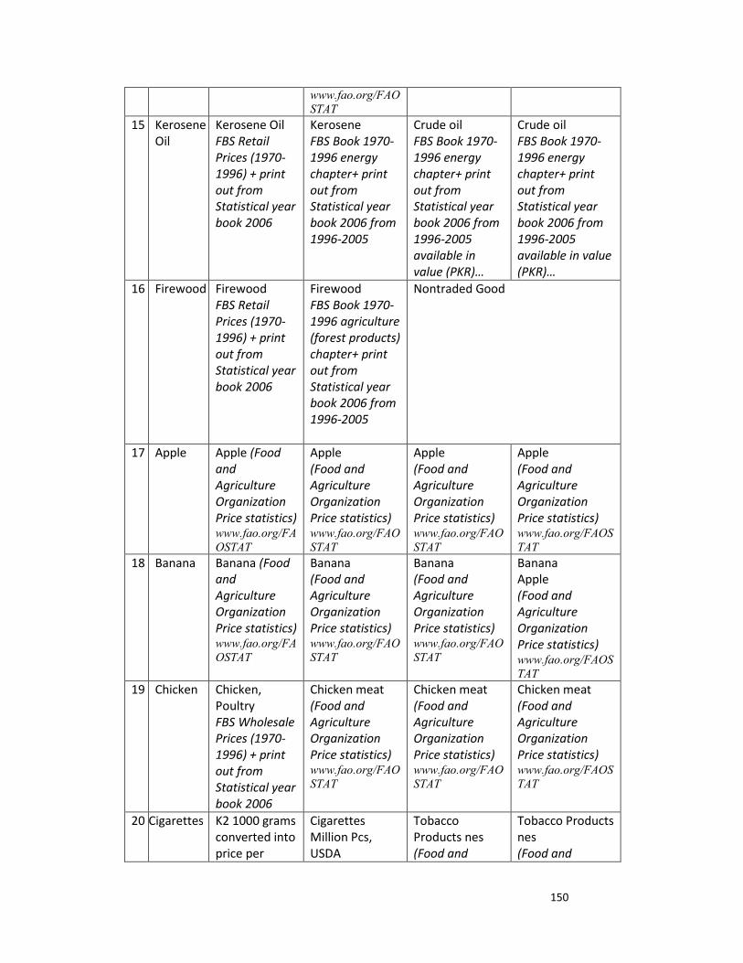
150

www.fao.org/FAOSTAT

15 Kerosene Oil

Kerosene Oil FBS Retail Prices (1970-1996) + print out from Statistical year book 2006

Kerosene FBS Book 1970-1996 energy chapter+ print out from Statistical year book 2006 from 1996-2005

Crude oil FBS Book 1970-1996 energy chapter+ print out from Statistical year book 2006 from 1996-2005 available in value (PKR)…

Crude oil FBS Book 1970-1996 energy chapter+ print out from Statistical year book 2006 from 1996-2005 available in value (PKR)…

16 Firewood Firewood FBS Retail Prices (1970-1996) + print out from Statistical year book 2006

Firewood FBS Book 1970-1996 agriculture (forest products) chapter+ print out from Statistical year book 2006 from 1996-2005

Nontraded Good

17 Apple Apple (Food and Agriculture Organization Price statistics) www.fao.org/FAOSTAT

Apple (Food and Agriculture Organization Price statistics) www.fao.org/FAOSTAT

Apple (Food and Agriculture Organization Price statistics) www.fao.org/FAOSTAT

Apple (Food and Agriculture Organization Price statistics) www.fao.org/FAOSTAT

18 Banana Banana (Food and Agriculture Organization Price statistics) www.fao.org/FAOSTAT

Banana (Food and Agriculture Organization Price statistics) www.fao.org/FAOSTAT

Banana (Food and Agriculture Organization Price statistics) www.fao.org/FAOSTAT

Banana Apple (Food and Agriculture Organization Price statistics) www.fao.org/FAOSTAT

19 Chicken Chicken, Poultry FBS Wholesale Prices (1970-1996) + print out from Statistical year book 2006

Chicken meat (Food and Agriculture Organization Price statistics) www.fao.org/FAOSTAT

Chicken meat (Food and Agriculture Organization Price statistics) www.fao.org/FAOSTAT

Chicken meat (Food and Agriculture Organization Price statistics) www.fao.org/FAOSTAT

20 Cigarettes K2 1000 grams converted into price per

Cigarettes Million Pcs, USDA

Tobacco Products nes (Food and

Tobacco Products nes (Food and

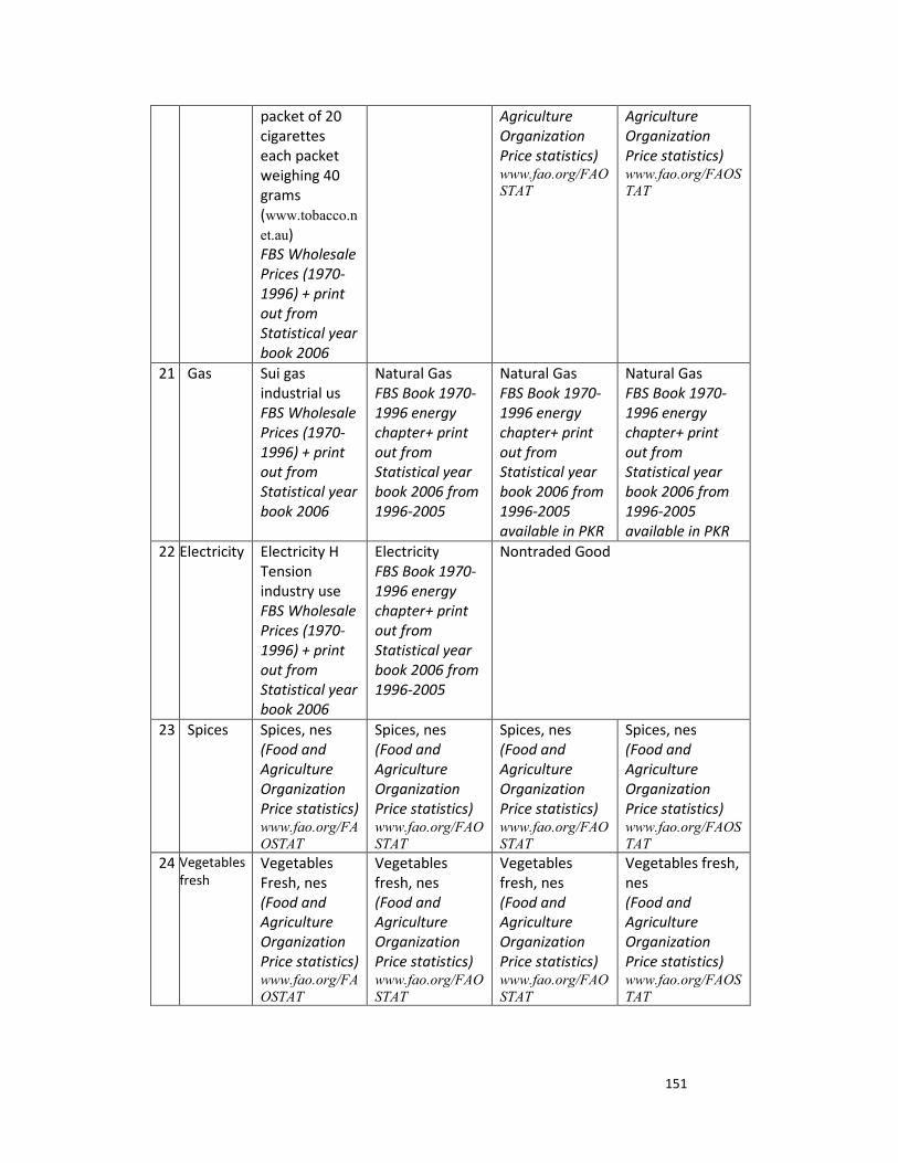
151

packet of 20 cigarettes each packet weighing 40 grams (www.tobacco.net.au) FBS Wholesale Prices (1970-1996) + print out from Statistical year book 2006

Agriculture Organization Price statistics) www.fao.org/FAOSTAT

Agriculture Organization Price statistics) www.fao.org/FAOSTAT

21 Gas Sui gas industrial us FBS Wholesale Prices (1970-1996) + print out from Statistical year book 2006

Natural Gas FBS Book 1970-1996 energy chapter+ print out from Statistical year book 2006 from 1996-2005

Natural Gas FBS Book 1970-1996 energy chapter+ print out from Statistical year book 2006 from 1996-2005 available in PKR

Natural Gas FBS Book 1970-1996 energy chapter+ print out from Statistical year book 2006 from 1996-2005 available in PKR

22 Electricity Electricity H Tension industry use FBS Wholesale Prices (1970-1996) + print out from Statistical year book 2006

Electricity FBS Book 1970-1996 energy chapter+ print out from Statistical year book 2006 from 1996-2005

Nontraded Good

23 Spices Spices, nes (Food and Agriculture Organization Price statistics) www.fao.org/FAOSTAT

Spices, nes (Food and Agriculture Organization Price statistics) www.fao.org/FAOSTAT

Spices, nes (Food and Agriculture Organization Price statistics) www.fao.org/FAOSTAT

Spices, nes (Food and Agriculture Organization Price statistics) www.fao.org/FAOSTAT

24 Vegetables fresh

Vegetables Fresh, nes (Food and Agriculture Organization Price statistics) www.fao.org/FAOSTAT

Vegetables fresh, nes (Food and Agriculture Organization Price statistics) www.fao.org/FAOSTAT

Vegetables fresh, nes (Food and Agriculture Organization Price statistics) www.fao.org/FAOSTAT

Vegetables fresh, nes (Food and Agriculture Organization Price statistics) www.fao.org/FAOSTAT

A1.3 Estimated Domestic Prices, Calculated Domestic Prices with Average Tariff Rates and Calculated Domestic Prices with Actual Tariff Rates for Available Years

Potatoes (PKR per ton)

Banana (PKR per ton)

Apple (PKR per ton)

Vegetable Oil (PKR per ton)

Pulses (PKR per ton)

Milk (PKR per ton)

Rice (PKR per ton)

Wheat (PKR per ton)

152

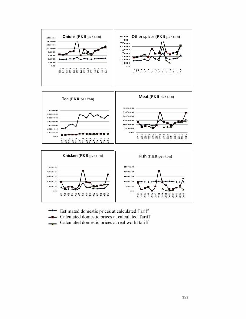
stimated domestic prices at calculated Tariff alculated domestic prices at calculated Tariff alculated domestic prices at real world tariff

ECC

Fish (PKR per ton)

Chicken (PKR per ton)

Meat (PKR per ton)

Tea (PKR per ton)

Other spices (PKR per ton)

Onions (PKR per ton)

153

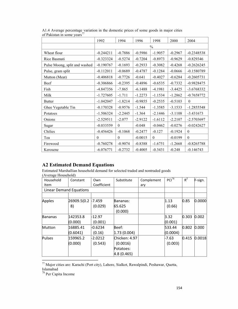
154

A1.4 Average percentage variation in the domestic prices of some goods in major cities of Pakistan in some years77

1992 1994 1996 1998 2000 2004

%

Wheat flour -0.244211 -0.7886 -0.5986 -1.9057 -0.2967 -0.2348538

Rice Basmati -0.323324 -0.5274 -0.7204 -0.8973 -0.9629 -0.829346

Pulse Moong, split and washed -0.190767 -0.1693 -0.2933 -0.3082 -0.4268 -0.2626245

Pulse, gram split -0.112011 -0.0689 -0.4787 -0.1284 -0.0666 -0.1580789

Mutton (Meat) -0.406818 -0.7726 -0.641 -0.4027 -0.6284 -0.2605731

Beef -0.306866 -0.2395 -0.4896 -0.6535 -0.7332 -0.9828475

Fish -4.847356 -7.865 -6.1488 -4.1981 -3.4425 -3.6768332

Milk -1.727605 -1.711 -1.2273 -1.1534 -1.2862 -0.7658772

Butter -1.042047 -1.8214 -0.9855 -0.2535 -0.5103 0

Ghee Vegetable Tin -0.170328 -0.9576 -1.544 -1.3585 -3.1533 -1.2855548

Potatoes -1.506324 -2.2445 -1.364 -2.1446 -3.1108 -3.431673

Onions -2.529511 -2.077 -2.9122 -1.6112 -2.2107 -2.5703697

Sugar -0.033559 0 -0.048 -0.0462 -0.0276 -0.0242627

Chilies -0.456426 -0.1068 -0.2477 -0.127 -0.1924 0

Tea 0 0 -0.0015 0 -0.0199 0

Firewood -0.760278 -0.9074 -0.8388 -1.6751 -1.2668 -0.8265788

Kerosene -6.076771 -0.2732 -0.4005 -0.3431 -0.248 -0.146743

A2 Estimated Demand Equations Estimated Marshallian household demand for selected traded and nontraded goods (Average Household)

Household Item

Constant Own Coefficient

Substitute Complementary

PCI78 R2 F-sign.

Linear Demand Equations

Apples 26909.5(0.28)

-7.459 (0.029)

Bananas: 65.625

(0.000)

1.13 (0.66)

0.85 0.0000

Bananas 142353.8 (0.000)

-12.97 (0.001)

3.32 (0.001)

0.303 0.002

Mutton 16885.41 (0.6041)

-0.6234 (0.16)

Beef: 1.73 (0.004)

533.44 (0.0004)

0.802 0.000

Pulses 159965.2 (0.000)

-2.0212 (0.543)

Chicken: 4.97 (0.0016)

Potatoes: 4.8 (0.465)

-7.63 (0.003)

0.415 0.0018

77 Major cities are: Karachi (Port city), Lahore, Sialkot, Rawalpindi, Peshawar, Quetta, Islamabad 78 Per Capita Income

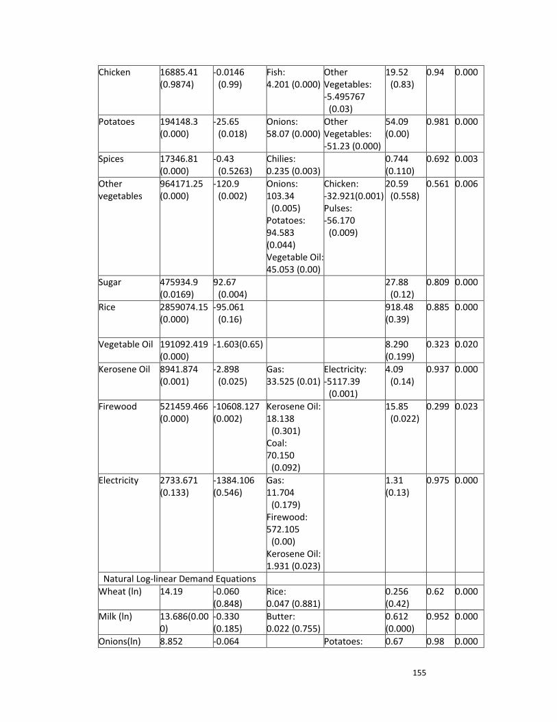
155

Chicken 16885.41 (0.9874)

-0.0146 (0.99)

Fish: 4.201 (0.000)

Other Vegetables: -5.495767

(0.03)

19.52 (0.83)

0.94 0.000

Potatoes 194148.3 (0.000)

-25.65 (0.018)

Onions: 58.07 (0.000)

Other Vegetables: -51.23 (0.000)

54.09 (0.00)

0.981 0.000

Spices 17346.81 (0.000)

-0.43 (0.5263)

Chilies: 0.235 (0.003)

0.744 (0.110)

0.692 0.003

Other vegetables

964171.25 (0.000)

-120.9 (0.002)

Onions: 103.34

(0.005) Potatoes: 94.583 (0.044) Vegetable Oil:45.053 (0.00)

Chicken: -32.921(0.001) Pulses: -56.170

(0.009)

20.59 (0.558)

0.561 0.006

Sugar 475934.9 (0.0169)

92.67 (0.004)

27.88 (0.12)

0.809 0.000

Rice 2859074.15 (0.000)

-95.061 (0.16)

918.48 (0.39)

0.885 0.000

Vegetable Oil 191092.419 (0.000)

-1.603(0.65) 8.290 (0.199)

0.323 0.020

Kerosene Oil 8941.874 (0.001)

-2.898 (0.025)

Gas: 33.525 (0.01)

Electricity: -5117.39

(0.001)

4.09 (0.14)

0.937 0.000

Firewood 521459.466 (0.000)

-10608.127 (0.002)

Kerosene Oil: 18.138

(0.301) Coal: 70.150

(0.092)

15.85 (0.022)

0.299 0.023

Electricity 2733.671 (0.133)

-1384.106 (0.546)

Gas: 11.704

(0.179) Firewood: 572.105

(0.00) Kerosene Oil: 1.931 (0.023)

1.31 (0.13)

0.975 0.000

Natural Log-linear Demand Equations Wheat (ln) 14.19 -0.060

(0.848) Rice: 0.047 (0.881)

0.256 (0.42)

0.62 0.000

Milk (ln) 13.686(0.000)

-0.330 (0.185)

Butter: 0.022 (0.755)

0.612 (0.000)

0.952 0.000

Onions(ln) 8.852 -0.064 Potatoes: 0.67 0.98 0.000

156

(0.000) (0.480) -0.116 (0.393) (0.000) Butter (ln) 9.385(0.000) -0.0221

(0.62) 0.38

(0.000) 0.95 0.000

Tea (ln) 8.503(0.009) -0.062 (0.889)

Cola: 0.048 (0.934)

0.46 (0.346)

0.62 0.0003

Cigarettes (ln) 10.793 (0.000)

-0.183 (0.167)

0.344 (0.001)

0.737 0.000

Gas(ln) 8.081 (0.000)

-0.054 (0.168)

Firewood: 0.143 (0.212)

0.516 (0.000)

0.9 0.000

Chilies (ln) 8.093 (0.000)

0.238(0.010) Other spices: 0.048 (0.817)

0.061 (0.664)

0.63 0.000

Beef (ln) 9.114 (0.000)

0.212(0.106) Fish: 0.14 (0.366)

Other Vegetables: -0.129(0.013)

0.18 (0.125)

0.97 0.000

Fish (ln) 8.620 (0.000)

0.688(0.016) Chicken: 0.253 (0.083)

Mutton -0.596 (0.113)

0.105 (0.666)

0.98 0.000

The values of error probability (t-significance) are presented in the parentheses in the cells with the estimates.

A3 Detailed tables on empirical estimations of demands and domestic prices including tariff

A 3.1 Estimated Marshallian Demands in tons for all selected traded and nontraded goods at actual import tariff rate

Wheat Milk Beef Fish Onion Chilies Tea

Tons

1992 1,471,055 904,267 236,697 242,056 20,445 71,276 -15,925

1993 1,473,980 907,957 76,707 60,163 24,380 63,064 -15,269

1994 1,476,638 920,657 114,725 102,346 27,583 73,132 -19,459

1995 1,478,190 933,682 121,673 126,304 29,351 86,754 -18,904

1996 1,480,880 951,040 55,379 41,473 33,614 79,689 -11,510

1997 1,482,536 969,937 149,312 151,690 28,211 105,663 -33,957

1998 1,486,195 963,098 525,779 591,097 39,161 100,326 -30,124

1999 1,495,928 970,977 96,461 99,220 50,378 87,318 -9,766

2000 1,497,192 957,401 80,894 72,830 55,821 122,741 -10,935

2001 1,496,467 974,526 82,241 73,054 59,060 82,225 1,453

2002 1,501,214 992,980 100,005 69,612 62,633 76,790 1,950

2003 1,508,646 971,732 144,355 119,816 70,191 108,715 -1,734

2004 1,515,279 1,008,669 150,586 157,614 78,608 117,108 11,797

2005 1,524,815 1,030,159 126,776 110,802 87,722 145,346 17,511

Gas Butter Rice Pulses Vegetable oil Apple Banana Meat

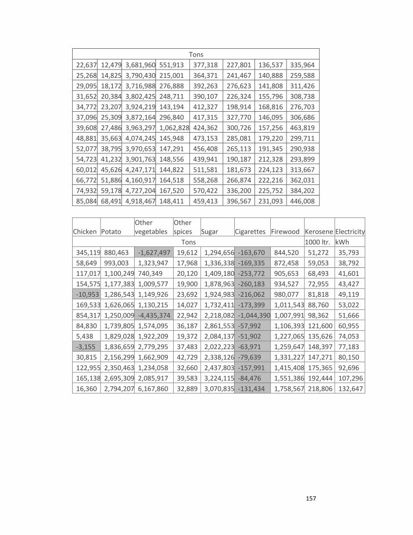
157

Tons 22,637 12,479 3,681,960 551,913 377,318 227,801 136,537 335,964 25,268 14,825 3,790,430 215,001 364,371 241,467 140,888 259,588 29,095 18,172 3,716,988 276,888 392,263 276,623 141,808 311,426 31,652 20,384 3,802,425 248,711 390,107 226,324 155,796 308,738 34,772 23,207 3,924,219 143,194 412,327 198,914 168,816 276,703 37,096 25,309 3,872,164 296,840 417,315 327,770 146,095 306,686 39,608 27,486 3,963,297 1,062,828 424,362 300,726 157,256 463,819 48,881 35,663 4,074,245 145,948 473,153 285,081 179,220 299,711 52,077 38,795 3,970,653 147,291 456,408 265,113 191,345 290,938 54,723 41,232 3,901,763 148,556 439,941 190,187 212,328 293,899 60,012 45,626 4,247,171 144,822 511,581 181,673 224,123 313,667 66,772 51,886 4,160,917 164,518 558,268 266,874 222,216 362,031 74,932 59,178 4,727,204 167,520 570,422 336,200 225,752 384,202 85,084 68,491 4,918,467 148,411 459,413 396,567 231,093 446,008

Chicken Potato Other vegetables

Other spices Sugar Cigarettes Firewood Kerosene Electricity

Tons 1000 ltr. kWh 345,119 880,463 -1,627,497 19,612 1,294,656 -163,670 844,520 51,272 35,793 58,649 993,003 1,323,947 17,968 1,336,338 -169,335 872,458 59,053 38,792 117,017 1,100,249 740,349 20,120 1,409,180 -253,772 905,653 68,493 41,601 154,575 1,177,383 1,009,577 19,900 1,878,963 -260,183 934,527 72,955 43,427 -10,953 1,286,543 1,149,926 23,692 1,924,983 -216,062 980,077 81,818 49,119 169,533 1,626,065 1,130,215 14,027 1,732,411 -173,399 1,011,543 88,760 53,022 854,317 1,250,009 -4,435,374 22,942 2,218,082 -1,044,390 1,007,991 98,362 51,666 84,830 1,739,805 1,574,095 36,187 2,861,553 -57,992 1,106,393 121,600 60,955 5,438 1,829,028 1,922,209 19,372 2,084,137 -51,902 1,227,065 135,626 74,053 -3,155 1,836,659 2,779,295 37,483 2,022,223 -63,971 1,259,647 148,397 77,183 30,815 2,156,299 1,662,909 42,729 2,338,126 -79,639 1,331,227 147,271 80,150 122,955 2,350,463 1,234,058 32,660 2,437,803 -157,991 1,415,408 175,365 92,696 165,138 2,695,309 2,085,917 39,583 3,224,115 -84,476 1,551,386 192,444 107,296 16,360 2,794,207 6,167,860 32,889 3,070,835 -131,434 1,758,567 218,806 132,647

158

A 3.2 Estimated Marshallian Demands in tons for all selected traded and nontraded goods at falling general import tariff rate Wheat Milk Beef Fish Onion Chilies Tea Tons

1992 1,471,055 904,267 236,697 242,056 20,445 71,276 -15,925

1993 1,473,980 907,952 73,315 56,132 24,662 60,704 -13,330

1994 1,476,640 920,664 117,422 105,519 27,419 74,402 -20,494

1995 1,478,190 933,677 121,209 125,755 29,385 86,480 -18,680

1996 1,480,876 951,008 54,555 40,209 34,202 74,412 -7,149

1997 1,482,533 969,746 120,941 118,061 30,420 87,345 -18,921

1998 1,486,186 962,934 357,038 397,490 40,639 88,240 -20,216

1999 1,494,774 973,543 177,530 182,598 48,386 96,651 -7,209

2000 1,496,184 963,973 144,719 136,631 54,815 128,028 -9,323

2001 1,496,210 975,984 93,679 78,867 59,026 88,433 4,213

2002 1,501,806 993,172 107,594 74,359 62,884 87,428 1,585

2003 1,508,440 971,355 129,528 102,564 70,757 97,174 8,253

2004 1,516,173 1,009,415 164,709 159,276 78,779 119,459 13,962

2005 1,524,284 1,030,605 258,830 250,988 88,837 142,269 18,593

Gas Butter Rice Pulses Vegetable oil Apple Banana Meat

Tons

22,637 12,479 3,681,961 551,913 377,318 227,801 136,537 335,964

25,270 14,825 3,790,692 207,264 365,439 232,477 142,893 257,996

29,094 18,172 3,714,861 282,889 391,706 281,865 140,639 312,679

31,653 20,384 3,802,488 247,663 390,208 225,225 156,041 308,521

34,778 23,207 3,927,972 140,000 414,671 180,219 172,986 276,203

37,113 25,309 3,875,244 232,520 422,140 257,482 161,772 293,401

39,618 27,486 3,971,486 709,807 427,292 253,700 167,745 387,336

48,885 35,663 4,171,263 286,580 475,871 221,224 193,462 340,441

52,079 38,795 4,041,684 233,213 467,199 222,364 200,880 321,505

54,725 41,232 3,857,923 127,116 452,015 137,932 223,983 300,210

60,024 45,626 4,238,806 120,985 525,256 153,297 230,452 320,727

66,787 51,886 4,345,051 132,394 564,753 248,867 226,232 355,216

74,946 59,178 4,474,798 144,201 581,699 315,873 230,286 394,748

85,107 68,491 5,009,917 368,020 472,535 384,163 233,859 508,013

Chicken Potato Other vegetables

Other spices Sugar Cigarettes Firewood Kerosene Electricity

Tons 1000 ltr. kWh

345,119 880,464 -1,627,497 19,612 1,294,655 -168,475 844,520 51,272 35,793

53,310 995,911 1,339,359 18,818 1,326,620 -143,034 871,988 59,070 38,718

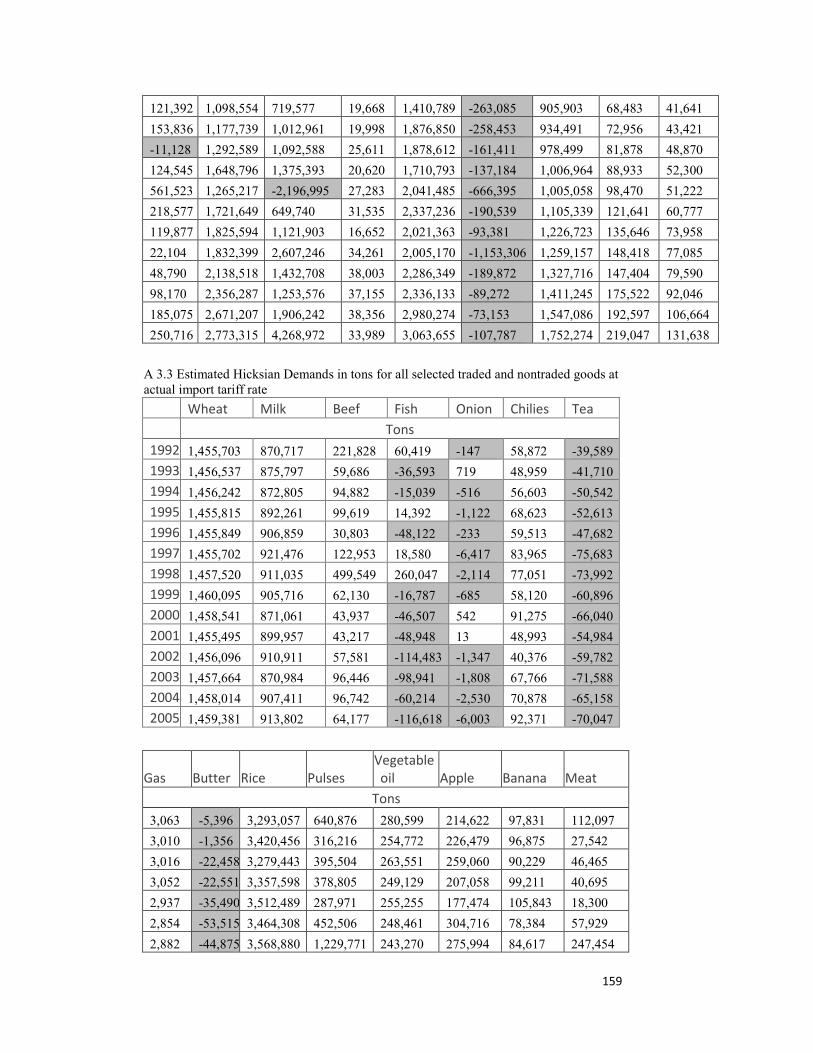
159

121,392 1,098,554 719,577 19,668 1,410,789 -263,085 905,903 68,483 41,641

153,836 1,177,739 1,012,961 19,998 1,876,850 -258,453 934,491 72,956 43,421

-11,128 1,292,589 1,092,588 25,611 1,878,612 -161,411 978,499 81,878 48,870

124,545 1,648,796 1,375,393 20,620 1,710,793 -137,184 1,006,964 88,933 52,300

561,523 1,265,217 -2,196,995 27,283 2,041,485 -666,395 1,005,058 98,470 51,222

218,577 1,721,649 649,740 31,535 2,337,236 -190,539 1,105,339 121,641 60,777

119,877 1,825,594 1,121,903 16,652 2,021,363 -93,381 1,226,723 135,646 73,958

22,104 1,832,399 2,607,246 34,261 2,005,170 -1,153,306 1,259,157 148,418 77,085

48,790 2,138,518 1,432,708 38,003 2,286,349 -189,872 1,327,716 147,404 79,590

98,170 2,356,287 1,253,576 37,155 2,336,133 -89,272 1,411,245 175,522 92,046

185,075 2,671,207 1,906,242 38,356 2,980,274 -73,153 1,547,086 192,597 106,664

250,716 2,773,315 4,268,972 33,989 3,063,655 -107,787 1,752,274 219,047 131,638

A 3.3 Estimated Hicksian Demands in tons for all selected traded and nontraded goods at actual import tariff rate Wheat Milk Beef Fish Onion Chilies Tea Tons 1992 1,455,703 870,717 221,828 60,419 -147 58,872 -39,589 1993 1,456,537 875,797 59,686 -36,593 719 48,959 -41,710 1994 1,456,242 872,805 94,882 -15,039 -516 56,603 -50,542 1995 1,455,815 892,261 99,619 14,392 -1,122 68,623 -52,613 1996 1,455,849 906,859 30,803 -48,122 -233 59,513 -47,682 1997 1,455,702 921,476 122,953 18,580 -6,417 83,965 -75,683 1998 1,457,520 911,035 499,549 260,047 -2,114 77,051 -73,992 1999 1,460,095 905,716 62,130 -16,787 -685 58,120 -60,896 2000 1,458,541 871,061 43,937 -46,507 542 91,275 -66,040 2001 1,455,495 899,957 43,217 -48,948 13 48,993 -54,984 2002 1,456,096 910,911 57,581 -114,483 -1,347 40,376 -59,782 2003 1,457,664 870,984 96,446 -98,941 -1,808 67,766 -71,588 2004 1,458,014 907,411 96,742 -60,214 -2,530 70,878 -65,158 2005 1,459,381 913,802 64,177 -116,618 -6,003 92,371 -70,047

Gas Butter Rice Pulses Vegetable oil Apple Banana Meat

Tons

3,063 -5,396 3,293,057 640,876 280,599 214,622 97,831 112,097

3,010 -1,356 3,420,456 316,216 254,772 226,479 96,875 27,542

3,016 -22,458 3,279,443 395,504 263,551 259,060 90,229 46,465

3,052 -22,551 3,357,598 378,805 249,129 207,058 99,211 40,695

2,937 -35,490 3,512,489 287,971 255,255 177,474 105,843 18,300

2,854 -53,515 3,464,308 452,506 248,461 304,716 78,384 57,929

2,882 -44,875 3,568,880 1,229,771 243,270 275,994 84,617 247,454

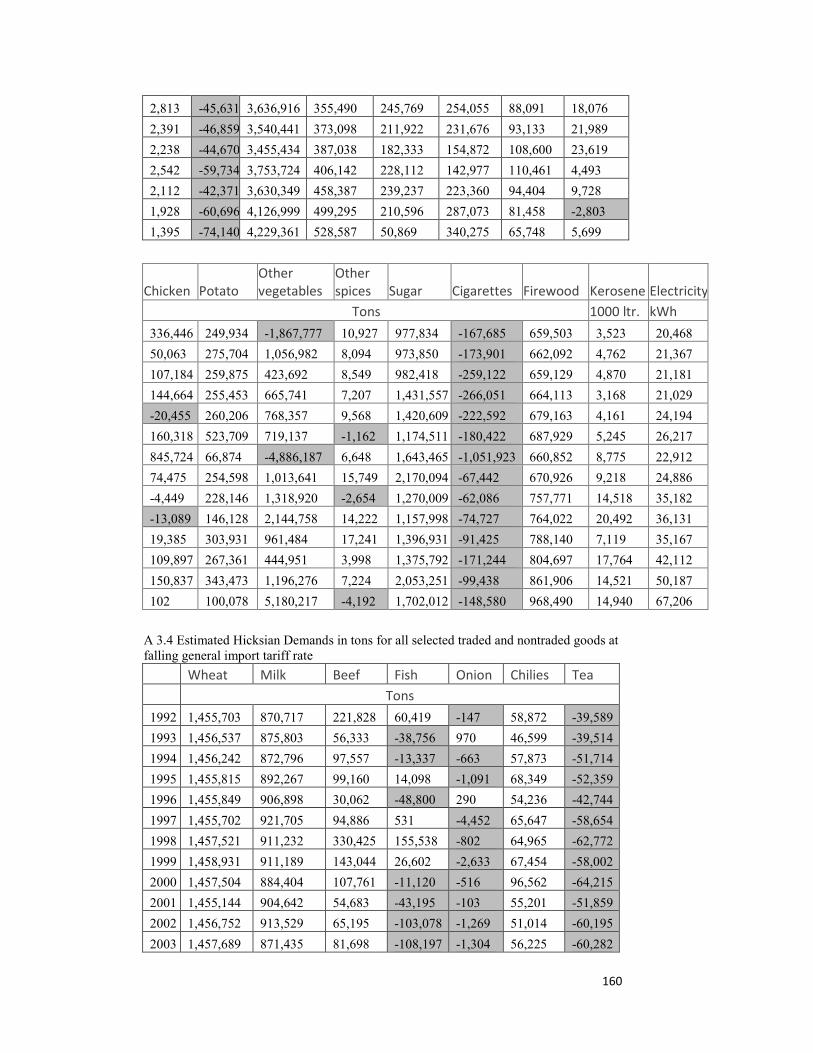
160

2,813 -45,631 3,636,916 355,490 245,769 254,055 88,091 18,076

2,391 -46,859 3,540,441 373,098 211,922 231,676 93,133 21,989

2,238 -44,670 3,455,434 387,038 182,333 154,872 108,600 23,619

2,542 -59,734 3,753,724 406,142 228,112 142,977 110,461 4,493

2,112 -42,371 3,630,349 458,387 239,237 223,360 94,404 9,728

1,928 -60,696 4,126,999 499,295 210,596 287,073 81,458 -2,803

1,395 -74,140 4,229,361 528,587 50,869 340,275 65,748 5,699

Chicken Potato Other vegetables

Other spices Sugar Cigarettes Firewood Kerosene Electricity

Tons 1000 ltr. kWh

336,446 249,934 -1,867,777 10,927 977,834 -167,685 659,503 3,523 20,468

50,063 275,704 1,056,982 8,094 973,850 -173,901 662,092 4,762 21,367

107,184 259,875 423,692 8,549 982,418 -259,122 659,129 4,870 21,181

144,664 255,453 665,741 7,207 1,431,557 -266,051 664,113 3,168 21,029

-20,455 260,206 768,357 9,568 1,420,609 -222,592 679,163 4,161 24,194

160,318 523,709 719,137 -1,162 1,174,511 -180,422 687,929 5,245 26,217

845,724 66,874 -4,886,187 6,648 1,643,465 -1,051,923 660,852 8,775 22,912

74,475 254,598 1,013,641 15,749 2,170,094 -67,442 670,926 9,218 24,886

-4,449 228,146 1,318,920 -2,654 1,270,009 -62,086 757,771 14,518 35,182

-13,089 146,128 2,144,758 14,222 1,157,998 -74,727 764,022 20,492 36,131

19,385 303,931 961,484 17,241 1,396,931 -91,425 788,140 7,119 35,167

109,897 267,361 444,951 3,998 1,375,792 -171,244 804,697 17,764 42,112

150,837 343,473 1,196,276 7,224 2,053,251 -99,438 861,906 14,521 50,187

102 100,078 5,180,217 -4,192 1,702,012 -148,580 968,490 14,940 67,206

A 3.4 Estimated Hicksian Demands in tons for all selected traded and nontraded goods at falling general import tariff rate Wheat Milk Beef Fish Onion Chilies Tea Tons

1992 1,455,703 870,717 221,828 60,419 -147 58,872 -39,589

1993 1,456,537 875,803 56,333 -38,756 970 46,599 -39,514

1994 1,456,242 872,796 97,557 -13,337 -663 57,873 -51,714

1995 1,455,815 892,267 99,160 14,098 -1,091 68,349 -52,359

1996 1,455,849 906,898 30,062 -48,800 290 54,236 -42,744

1997 1,455,702 921,705 94,886 531 -4,452 65,647 -58,654

1998 1,457,521 911,232 330,425 155,538 -802 64,965 -62,772

1999 1,458,931 911,189 143,044 26,602 -2,633 67,454 -58,002

2000 1,457,504 884,404 107,761 -11,120 -516 96,562 -64,215

2001 1,455,144 904,642 54,683 -43,195 -103 55,201 -51,859

2002 1,456,752 913,529 65,195 -103,078 -1,269 51,014 -60,195

2003 1,457,689 871,435 81,698 -108,197 -1,304 56,225 -60,282

161

2004 1,458,668 910,500 110,887 -61,528 -2,580 73,229 -62,708

2005 1,458,910 917,317 196,328 -40,137 -5,160 89,294 -68,822

Gas Butter Rice Pulses Vegetable oil Apple Banana Meat

Tons

3,063 -5,396 3,293,057 640,876 280,599 214,621 97,831 112,097

3,012 -1,338 3,420,697 308,480 255,828 217,490 98,879 25,889

3,015 -22,484 3,277,442 401,505 262,998 264,302 89,061 47,776

3,053 -22,532 3,357,658 377,758 249,229 205,959 99,456 40,470

2,943 -35,383 3,516,003 284,777 257,580 158,779 110,012 17,789

2,872 -52,873 3,467,228 388,193 253,244 234,427 94,056 44,166

2,894 -44,322 3,576,592 876,760 246,173 228,967 95,103 161,289

2,818 -45,060 3,727,931 496,121 248,466 190,197 102,330 59,473

2,393 -46,073 3,608,003 459,019 222,587 188,927 102,666 52,979

2,240 -42,649 3,413,184 365,598 194,234 102,618 120,253 29,931

2,557 -57,310 3,745,790 382,305 241,670 114,600 116,789 11,406

2,128 -41,099 3,802,485 426,263 245,679 205,353 98,419 2,701

1,944 -58,919 3,889,804 475,976 221,770 266,746 85,990 7,814

1,420 -71,280 4,315,512 748,196 63,742 327,871 68,514 69,211

Chicken Potato Other vegetables

Other spices Sugar Cigarettes Firewood Kerosene Electricity

Tons 1000 ltr. kWh

336,446 249,934 -1,867,776 10,927 977,834 -172,490 659,503 3,523 20,468

44,724 278,585 1,072,179 8,944 963,983 -147,599 661,623 4,780 21,293

111,560 258,199 402,985 8,097 984,050 -268,435 659,378 4,861 21,221

143,925 255,805 669,104 7,305 1,429,379 -264,322 664,077 3,169 21,023

-20,630 266,207 710,610 11,487 1,372,982 -167,941 677,585 4,220 23,945

115,328 546,035 962,865 5,431 1,152,538 -144,207 683,350 5,417 25,495

552,752 81,891 -2,647,808 10,990 1,461,256 -673,928 657,919 8,882 22,468

208,223 236,665 89,830 11,097 1,621,670 -199,989 669,872 9,259 24,708

109,991 224,807 518,635 -5,375 1,206,328 -103,565 757,428 14,538 35,086

12,170 141,890 1,972,546 11,001 1,140,754 -1,164,061 763,531 20,514 36,033

37,361 286,163 731,219 12,515 1,344,354 -201,657 784,630 7,252 34,607

85,112 273,137 464,296 8,493 1,272,731 -102,525 800,534 17,920 41,462

170,774 319,405 1,016,535 5,997 1,802,766 -88,115 857,607 14,675 49,555

234,458 79,097 3,280,190 -3,092 1,694,708 -124,933 962,197 15,180 66,196

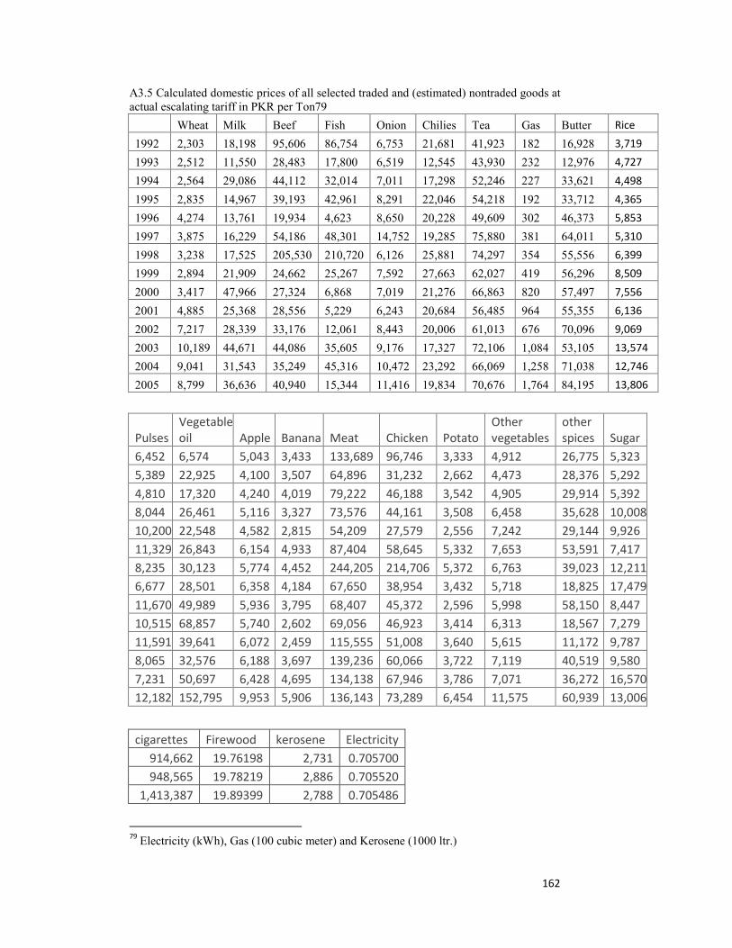
162

A3.5 Calculated domestic prices of all selected traded and (estimated) nontraded goods at actual escalating tariff in PKR per Ton79

Wheat Milk Beef Fish Onion Chilies Tea Gas Butter Rice

1992 2,303 18,198 95,606 86,754 6,753 21,681 41,923 182 16,928 3,719

1993 2,512 11,550 28,483 17,800 6,519 12,545 43,930 232 12,976 4,727

1994 2,564 29,086 44,112 32,014 7,011 17,298 52,246 227 33,621 4,498

1995 2,835 14,967 39,193 42,961 8,291 22,046 54,218 192 33,712 4,365

1996 4,274 13,761 19,934 4,623 8,650 20,228 49,609 302 46,373 5,853

1997 3,875 16,229 54,186 48,301 14,752 19,285 75,880 381 64,011 5,310

1998 3,238 17,525 205,530 210,720 6,126 25,881 74,297 354 55,556 6,399

1999 2,894 21,909 24,662 25,267 7,592 27,663 62,027 419 56,296 8,509

2000 3,417 47,966 27,324 6,868 7,019 21,276 66,863 820 57,497 7,556

2001 4,885 25,368 28,556 5,229 6,243 20,684 56,485 964 55,355 6,136

2002 7,217 28,339 33,176 12,061 8,443 20,006 61,013 676 70,096 9,069

2003 10,189 44,671 44,086 35,605 9,176 17,327 72,106 1,084 53,105 13,574

2004 9,041 31,543 35,249 45,316 10,472 23,292 66,069 1,258 71,038 12,746

2005 8,799 36,636 40,940 15,344 11,416 19,834 70,676 1,764 84,195 13,806

Pulses Vegetable oil Apple Banana Meat Chicken Potato

Other vegetables

other spices Sugar

6,452 6,574 5,043 3,433 133,689 96,746 3,333 4,912 26,775 5,323 5,389 22,925 4,100 3,507 64,896 31,232 2,662 4,473 28,376 5,292 4,810 17,320 4,240 4,019 79,222 46,188 3,542 4,905 29,914 5,392 8,044 26,461 5,116 3,327 73,576 44,161 3,508 6,458 35,628 10,00810,200 22,548 4,582 2,815 54,209 27,579 2,556 7,242 29,144 9,926 11,329 26,843 6,154 4,933 87,404 58,645 5,332 7,653 53,591 7,417 8,235 30,123 5,774 4,452 244,205 214,706 5,372 6,763 39,023 12,2116,677 28,501 6,358 4,184 67,650 38,954 3,432 5,718 18,825 17,47911,670 49,989 5,936 3,795 68,407 45,372 2,596 5,998 58,150 8,447 10,515 68,857 5,740 2,602 69,056 46,923 3,414 6,313 18,567 7,279 11,591 39,641 6,072 2,459 115,555 51,008 3,640 5,615 11,172 9,787 8,065 32,576 6,188 3,697 139,236 60,066 3,722 7,119 40,519 9,580 7,231 50,697 6,428 4,695 134,138 67,946 3,786 7,071 36,272 16,57012,182 152,795 9,953 5,906 136,143 73,289 6,454 11,575 60,939 13,006

cigarettes Firewood kerosene Electricity 914,662 19.76198 2,731 0.705700 948,565 19.78219 2,886 0.705520

1,413,387 19.89399 2,788 0.705486

79 Electricity (kWh), Gas (100 cubic meter) and Kerosene (1000 ltr.)

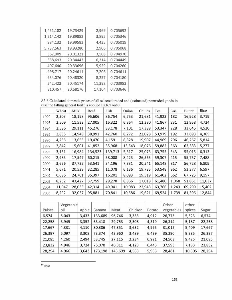
163

1,451,182 19.73429 2,969 0.705692 1,214,142 19.89882 3,895 0.705346

984,132 19.99583 4,435 0.705019 5,737,563 19.93280 2,906 0.705068

367,909 20.01321 3,508 0.704970 338,693 20.34443 6,314 0.704449 407,640 20.33696 5,929 0.704260 498,717 20.24611 7,206 0.704611 934,076 20.48320 8,257 0.704180 542,423 20.45174 11,393 0.703983 810,457 20.58176 17,104 0.703646

A3.6 Calculated domestic prices of all selected traded and (estimated) nontraded goods in case the falling general tariff is applied PKR/Ton80

Wheat Milk Beef Fish Onion Chilies Tea Gas Butter Rice

1992 2,303 18,198 95,606 86,754 6,753 21,681 41,923 182 16,928 3,719

1993 2,509 11,532 27,005 16,322 6,364 12,390 41,867 231 12,958 4,724

1994 2,586 29,111 45,276 33,178 7,101 17,388 53,347 228 33,646 4,520

1995 2,835 14,948 38,991 42,760 8,272 22,028 53,979 192 33,693 4,365

1996 4,235 13,655 19,470 4,159 8,328 19,907 44,969 296 46,267 5,814

1997 3,842 15,601 41,852 35,968 13,543 18,076 59,882 363 63,383 5,277

1998 3,151 16,984 134,523 139,713 5,317 25,073 63,755 343 55,015 6,313

1999 2,983 17,547 60,215 58,008 8,423 26,565 59,307 415 55,737 7,488

2000 3,656 37,735 53,541 34,196 7,331 20,541 65,148 817 56,728 6,809

2001 5,671 20,529 32,285 11,078 6,136 19,785 53,548 962 53,377 6,597

2002 6,686 24,701 35,397 16,201 8,093 19,519 61,402 662 67,725 9,157

2003 8,252 43,427 37,759 29,278 8,866 17,018 61,480 1,068 51,861 11,637

2004 11,047 28,033 42,314 49,941 10,083 22,943 63,766 1,243 69,299 15,402

2005 8,292 32,037 95,881 70,841 10,586 19,621 69,524 1,739 81,396 12,844

Pulses Vegetable oil Apple Banana Meat Chicken Potato

Other vegetables

other spices Sugar

6,574 5,043 3,433 133,689 96,746 3,333 4,912 26,775 5,323 6,574 22,258 3,945 3,352 63,418 29,753 2,508 4,319 26,314 5,187 22,258 17,667 4,331 4,110 80,386 47,351 3,632 4,995 31,015 5,409 17,667 26,397 5,097 3,308 73,374 43,960 3,489 6,439 35,390 9,985 26,397 21,085 4,260 2,494 53,745 27,115 2,234 6,921 24,503 9,425 21,085 23,832 4,946 3,724 75,070 46,311 4,123 6,445 37,593 7,183 23,832 28,294 4,966 3,643 173,198 143,699 4,563 5,955 28,481 10,305 28,294

80 Ibid

164

26,805 5,260 3,086 99,295 66,649 4,793 6,333 29,049 11,820 26,805 43,255 5,201 3,060 90,889 62,310 3,397 6,018 64,078 7,770 43,255 61,322 4,842 1,704 69,103 42,420 3,565 6,200 25,570 7,095 61,322 31,108 5,584 1,971 110,287 46,043 3,727 5,522 21,902 9,229 31,108 28,529 5,878 3,387 132,909 53,739 3,413 6,809 29,893 8,482 28,529 43,660 6,079 4,346 136,494 63,101 4,004 6,991 38,935 13,938 43,660 144,607 9,740 5,693 186,551 117,965 6,075 11,231 58,264 12,929 144,607

Cigarettes Firewood kerosene Electricity 940,873 19.761978 2,731 0.705700 805,110 19.780347 2,859 0.705535 1,464,182 19.895468 2,802 0.705479 1,441,748 19.734006 2,967 0.705694 916,060 19.892632 3,805 0.705382 786,606 19.978764 4,173 0.705106 3,675,863 19.930211 2,742 0.705127 1,090,859 20.003891 3,444 0.705009 564,932 20.323900 6,283 0.704462 6,349,196 20.325435 5,896 0.704350 1,099,957 20.230000 7,003 0.704700 559,261 20.470455 8,020 0.704185 480,666 20.457123 11,159 0.704028 681,479 20.550137 16,738 0.703656

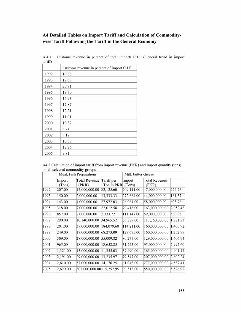
165

A4 Detailed Tables on Import Tariff and Calculation of Commodity-wise Tariff Following the Tariff in the General Economy

A 4.1 Customs revenue in percent of total imports C.I.F (General trend in import tariff)

Customs revenue in percent of import C.I.F

1992 19.88

1993 17.68

1994 20.71

1995 19.70

1996 15.93

1997 12.87

1998 12.21

1999 11.01

2000 10.37

2001 6.74

2002 9.17

2003 10.38

2004 12.26

2005 9.81

A4.2 Calculation of import tariff from import revenue (PKR) and import quantity (tons) on all selected commodity groups

Meat, Fish Preparations Milk butter cheese

Import (Tons)

Total Revenue (PKR)

Tariff per Ton in PKR

Import (Tons)

Total Revenue (PKR)

1992 207.00 17,000,000.00 82,125.60 209,111.00 47,000,000.00 224.76

1993 150.00 2,000,000.00 13,333.33 272,664.00 44,000,000.00 161.37

1994 143.00 4,000,000.00 27,972.03 96,064.00 58,000,000.00 603.76

1995 318.00 7,000,000.00 22,012.58 79,416.00 163,000,000.00 2,052.48

1996 857.00 2,000,000.00 2,333.72 111,147.00 59,000,000.00 530.83

1997 290.00 10,140,000.00 34,965.52 65,887.00 117,360,000.00 1,781.23

1998 201.00 37,000,000.00 184,079.60 114,211.00 160,000,000.00 1,400.92

1999 249.00 17,000,000.00 68,273.09 127,695.00 160,000,000.00 1,252.99

2000 509.00 28,000,000.00 55,009.82 80,277.00 129,000,000.00 1,606.94

2001 965.00 18,000,000.00 18,652.85 31,745.00 95,000,000.00 2,992.60

2002 1,321.00 15,000,000.00 11,355.03 37,490.00 165,000,000.00 4,401.17

2003 2,191.00 29,000,000.00 13,235.97 79,547.00 207,000,000.00 2,602.24

2004 2,610.00 37,000,000.00 14,176.25 61,048.00 277,000,000.00 4,537.41

2005 2,629.00 303,000,000.00115,252.95 99,513.00 550,000,000.00 5,526.92

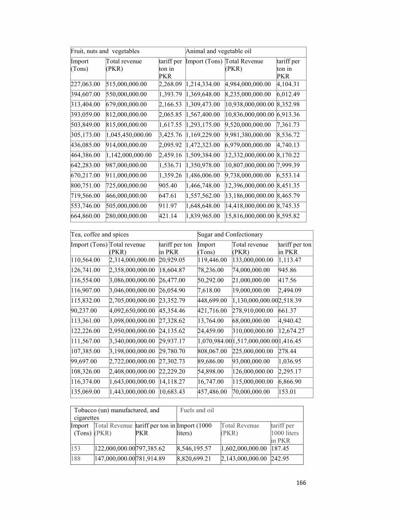
166

Fruit, nuts and vegetables Animal and vegetable oil

Import (Tons)

Total revenue (PKR)

tariff per ton in PKR

Import (Tons) Total Revenue (PKR)

tariff per ton in PKR

227,063.00 515,000,000.00 2,268.09 1,214,334.00 4,984,000,000.00 4,104.31

394,607.00 550,000,000.00 1,393.79 1,369,648.00 8,235,000,000.00 6,012.49

313,404.00 679,000,000.00 2,166.53 1,309,473.00 10,938,000,000.00 8,352.98

393,059.00 812,000,000.00 2,065.85 1,567,400.00 10,836,000,000.00 6,913.36

503,849.00 815,000,000.00 1,617.55 1,293,175.00 9,520,000,000.00 7,361.73

305,173.00 1,045,450,000.00 3,425.76 1,169,229.00 9,981,380,000.00 8,536.72

436,085.00 914,000,000.00 2,095.92 1,472,323.00 6,979,000,000.00 4,740.13

464,386.00 1,142,000,000.00 2,459.16 1,509,384.00 12,332,000,000.00 8,170.22

642,283.00 987,000,000.00 1,536.71 1,350,978.00 10,807,000,000.00 7,999.39

670,217.00 911,000,000.00 1,359.26 1,486,006.00 9,738,000,000.00 6,553.14

800,751.00 725,000,000.00 905.40 1,466,748.00 12,396,000,000.00 8,451.35

719,566.00 466,000,000.00 647.61 1,557,562.00 13,186,000,000.00 8,465.79

553,746.00 505,000,000.00 911.97 1,648,648.00 14,418,000,000.00 8,745.35

664,860.00 280,000,000.00 421.14 1,839,965.00 15,816,000,000.00 8,595.82

Tea, coffee and spices Sugar and Confectionary

Import (Tons) Total revenue (PKR)

tariff per ton in PKR

Import (Tons)

Total revenue (PKR)

tariff per ton in PKR

110,564.00 2,314,000,000.00 20,929.05 119,446.00 133,000,000.00 1,113.47

126,741.00 2,358,000,000.00 18,604.87 78,236.00 74,000,000.00 945.86

116,554.00 3,086,000,000.00 26,477.00 50,292.00 21,000,000.00 417.56

116,907.00 3,046,000,000.00 26,054.90 7,618.00 19,000,000.00 2,494.09

115,832.00 2,705,000,000.00 23,352.79 448,699.00 1,130,000,000.002,518.39

90,237.00 4,092,650,000.00 45,354.46 421,716.00 278,910,000.00 661.37

113,361.00 3,098,000,000.00 27,328.62 13,764.00 68,000,000.00 4,940.42

122,226.00 2,950,000,000.00 24,135.62 24,459.00 310,000,000.00 12,674.27

111,567.00 3,340,000,000.00 29,937.17 1,070,984.001,517,000,000.001,416.45

107,385.00 3,198,000,000.00 29,780.70 808,067.00 225,000,000.00 278.44

99,697.00 2,722,000,000.00 27,302.73 89,686.00 93,000,000.00 1,036.95

108,326.00 2,408,000,000.00 22,229.20 54,898.00 126,000,000.00 2,295.17

116,374.00 1,643,000,000.00 14,118.27 16,747.00 115,000,000.00 6,866.90

135,069.00 1,443,000,000.00 10,683.43 457,486.00 70,000,000.00 153.01

Tobacco (un) manufactured, and cigarettes

Fuels and oil

Import (Tons)

Total Revenue (PKR)

tariff per ton in PKR

Import (1000 liters)

Total Revenue (PKR)

tariff per 1000 liters in PKR

153 122,000,000.00797,385.62 8,546,195.57 1,602,000,000.00 187.45

188 147,000,000.00781,914.89 8,820,699.21 2,143,000,000.00 242.95

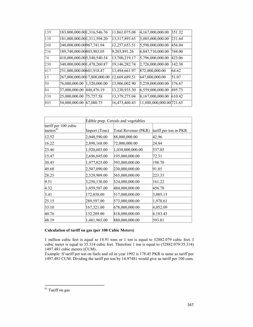
167

139 183,000,000.001,316,546.76 11,861,075.08 4,167,000,000.00 351.32

138 181,000,000.001,311,594.20 13,317,895.65 3,085,000,000.00 231.64

248 240,000,000.00967,741.94 12,257,653.51 5,590,000,000.00 456.04

236 189,740,000.00803,983.05 9,203,891.26 6,847,710,000.00 744.00

74 410,000,000.005,540,540.54 13,700,219.17 5,796,000,000.00 423.06

230 340,000,000.001,478,260.87 19,146,282.74 2,726,000,000.00 142.38

417 251,000,000.00601,918.47 13,494,661.97 872,000,000.00 64.62

15 267,000,000.0017,800,000.00 12,669,689.51 647,000,000.00 51.07

50 76,000,000.00 1,520,000.00 13,906,002.90 5,238,000,000.00 376.67

84 37,000,000.00 440,476.19 13,230,935.30 6,559,000,000.00 495.73

330 25,000,000.00 75,757.58 13,379,275.04 8,167,000,000.00 610.42

805 54,000,000.00 67,080.75 16,473,460.43 11,888,000,000.00 721.65

Edible prep. Cereals and vegetables tariff per 100 cubic meters81 Import (Tons) Total Revenue (PKR) tariff per ton in PKR

12.52 2,048,590.00 88,000,000.00 42.96

16.22 2,898,168.00 72,000,000.00 24.84

23.46 1,920,603.00 1,030,000,000.00 537.85

15.47 2,696,845.00 195,000,000.00 72.31

30.45 1,977,825.00 393,000,000.00 198.70

49.68 2,507,090.00 230,000,000.00 91.85

28.25 2,529,909.00 565,000,000.00 223.33

9.51 3,250,130.00 524,000,000.00 161.22

4.32 1,059,587.00 484,000,000.00 456.78

3.41 172,038.00 517,000,000.00 3,005.15

25.15 289,597.00 573,000,000.00 1,978.61

33.10 167,321.00 678,000,000.00 4,052.09

40.76 132,289.00 818,000,000.00 6,183.43

48.19 1,481,965.00 880,000,000.00 593.81 Calculation of tariff on gas (per 100 Cubic Meters) 1 million cubic feet is equal to 18.91 tons or 1 ton is equal to 52882.079 cubic feet. I cubic meter is equal to 35.314 cubic feet. Therefore 1 ton is equal to (52882.079/35.314) 1497.481 cubic meters (CUM). Example: If tariff per ton on fuels and oil in year 1992 is 178.45 PKR is same as tariff per 1497.481 CUM. Dividing the tariff per ton by 14.97481 would give us tariff per 100 cum.

81 Tariff on gas

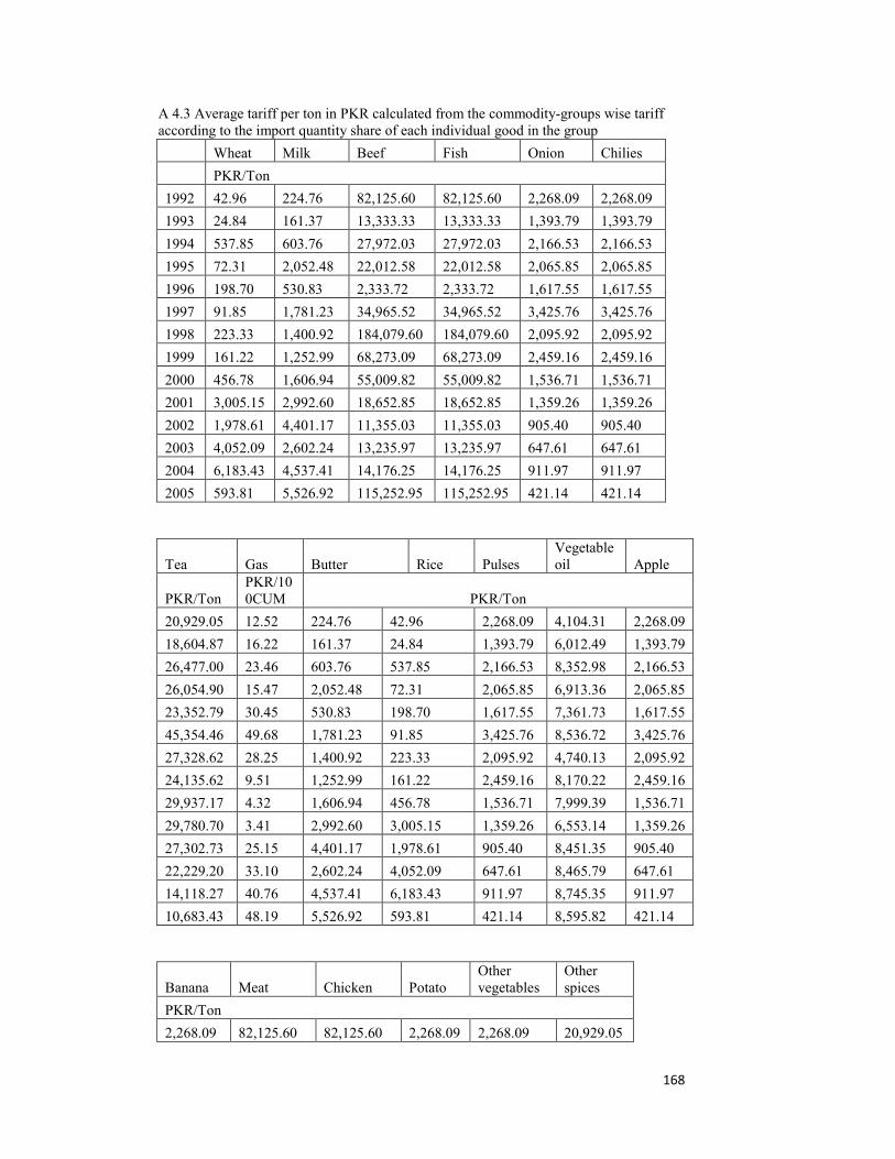
168

A 4.3 Average tariff per ton in PKR calculated from the commodity-groups wise tariff according to the import quantity share of each individual good in the group

Wheat Milk Beef Fish Onion Chilies

PKR/Ton

1992 42.96 224.76 82,125.60 82,125.60 2,268.09 2,268.09

1993 24.84 161.37 13,333.33 13,333.33 1,393.79 1,393.79

1994 537.85 603.76 27,972.03 27,972.03 2,166.53 2,166.53

1995 72.31 2,052.48 22,012.58 22,012.58 2,065.85 2,065.85

1996 198.70 530.83 2,333.72 2,333.72 1,617.55 1,617.55

1997 91.85 1,781.23 34,965.52 34,965.52 3,425.76 3,425.76

1998 223.33 1,400.92 184,079.60 184,079.60 2,095.92 2,095.92

1999 161.22 1,252.99 68,273.09 68,273.09 2,459.16 2,459.16

2000 456.78 1,606.94 55,009.82 55,009.82 1,536.71 1,536.71

2001 3,005.15 2,992.60 18,652.85 18,652.85 1,359.26 1,359.26

2002 1,978.61 4,401.17 11,355.03 11,355.03 905.40 905.40

2003 4,052.09 2,602.24 13,235.97 13,235.97 647.61 647.61

2004 6,183.43 4,537.41 14,176.25 14,176.25 911.97 911.97

2005 593.81 5,526.92 115,252.95 115,252.95 421.14 421.14

Tea Gas Butter Rice Pulses Vegetable oil Apple

PKR/Ton PKR/100CUM PKR/Ton

20,929.05 12.52 224.76 42.96 2,268.09 4,104.31 2,268.09

18,604.87 16.22 161.37 24.84 1,393.79 6,012.49 1,393.79

26,477.00 23.46 603.76 537.85 2,166.53 8,352.98 2,166.53

26,054.90 15.47 2,052.48 72.31 2,065.85 6,913.36 2,065.85

23,352.79 30.45 530.83 198.70 1,617.55 7,361.73 1,617.55

45,354.46 49.68 1,781.23 91.85 3,425.76 8,536.72 3,425.76

27,328.62 28.25 1,400.92 223.33 2,095.92 4,740.13 2,095.92

24,135.62 9.51 1,252.99 161.22 2,459.16 8,170.22 2,459.16

29,937.17 4.32 1,606.94 456.78 1,536.71 7,999.39 1,536.71

29,780.70 3.41 2,992.60 3,005.15 1,359.26 6,553.14 1,359.26

27,302.73 25.15 4,401.17 1,978.61 905.40 8,451.35 905.40

22,229.20 33.10 2,602.24 4,052.09 647.61 8,465.79 647.61

14,118.27 40.76 4,537.41 6,183.43 911.97 8,745.35 911.97

10,683.43 48.19 5,526.92 593.81 421.14 8,595.82 421.14

Banana Meat Chicken Potato Other vegetables

Other spices

PKR/Ton

2,268.09 82,125.60 82,125.60 2,268.09 2,268.09 20,929.05

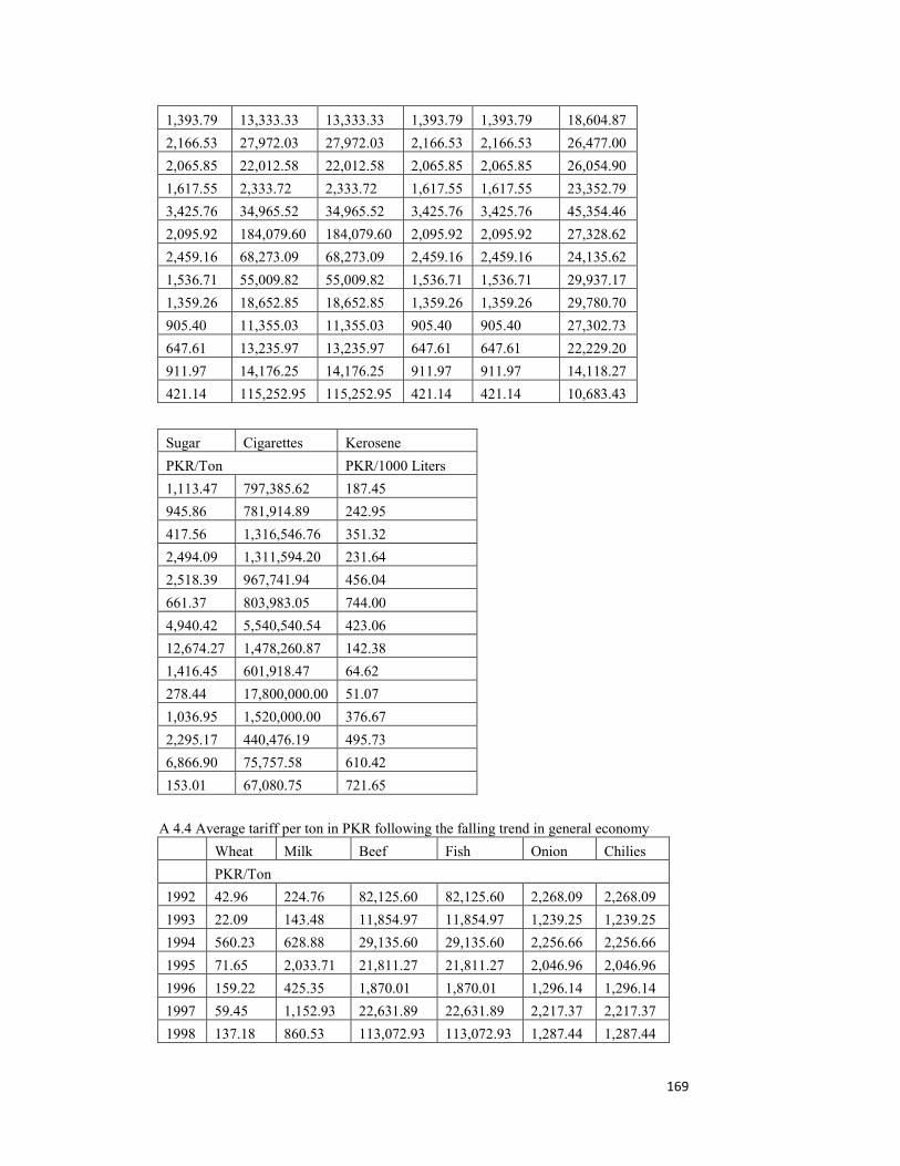
169

1,393.79 13,333.33 13,333.33 1,393.79 1,393.79 18,604.87

2,166.53 27,972.03 27,972.03 2,166.53 2,166.53 26,477.00

2,065.85 22,012.58 22,012.58 2,065.85 2,065.85 26,054.90

1,617.55 2,333.72 2,333.72 1,617.55 1,617.55 23,352.79

3,425.76 34,965.52 34,965.52 3,425.76 3,425.76 45,354.46

2,095.92 184,079.60 184,079.60 2,095.92 2,095.92 27,328.62

2,459.16 68,273.09 68,273.09 2,459.16 2,459.16 24,135.62

1,536.71 55,009.82 55,009.82 1,536.71 1,536.71 29,937.17

1,359.26 18,652.85 18,652.85 1,359.26 1,359.26 29,780.70

905.40 11,355.03 11,355.03 905.40 905.40 27,302.73

647.61 13,235.97 13,235.97 647.61 647.61 22,229.20

911.97 14,176.25 14,176.25 911.97 911.97 14,118.27

421.14 115,252.95 115,252.95 421.14 421.14 10,683.43

Sugar Cigarettes Kerosene

PKR/Ton PKR/1000 Liters

1,113.47 797,385.62 187.45

945.86 781,914.89 242.95

417.56 1,316,546.76 351.32

2,494.09 1,311,594.20 231.64

2,518.39 967,741.94 456.04

661.37 803,983.05 744.00

4,940.42 5,540,540.54 423.06

12,674.27 1,478,260.87 142.38

1,416.45 601,918.47 64.62

278.44 17,800,000.00 51.07

1,036.95 1,520,000.00 376.67

2,295.17 440,476.19 495.73

6,866.90 75,757.58 610.42

153.01 67,080.75 721.65

A 4.4 Average tariff per ton in PKR following the falling trend in general economy

Wheat Milk Beef Fish Onion Chilies

PKR/Ton

1992 42.96 224.76 82,125.60 82,125.60 2,268.09 2,268.09

1993 22.09 143.48 11,854.97 11,854.97 1,239.25 1,239.25

1994 560.23 628.88 29,135.60 29,135.60 2,256.66 2,256.66

1995 71.65 2,033.71 21,811.27 21,811.27 2,046.96 2,046.96

1996 159.22 425.35 1,870.01 1,870.01 1,296.14 1,296.14

1997 59.45 1,152.93 22,631.89 22,631.89 2,217.37 2,217.37

1998 137.18 860.53 113,072.93 113,072.93 1,287.44 1,287.44

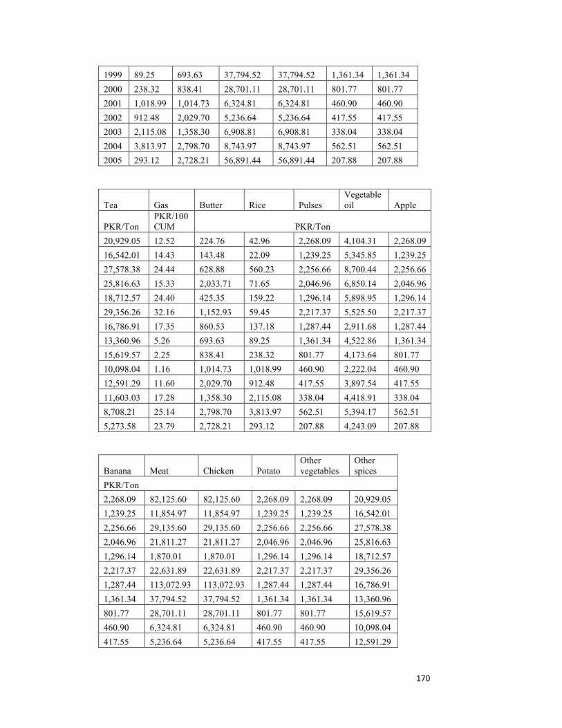
170

1999 89.25 693.63 37,794.52 37,794.52 1,361.34 1,361.34

2000 238.32 838.41 28,701.11 28,701.11 801.77 801.77

2001 1,018.99 1,014.73 6,324.81 6,324.81 460.90 460.90

2002 912.48 2,029.70 5,236.64 5,236.64 417.55 417.55

2003 2,115.08 1,358.30 6,908.81 6,908.81 338.04 338.04

2004 3,813.97 2,798.70 8,743.97 8,743.97 562.51 562.51

2005 293.12 2,728.21 56,891.44 56,891.44 207.88 207.88

Tea Gas Butter Rice Pulses Vegetable oil Apple

PKR/Ton PKR/100CUM PKR/Ton

20,929.05 12.52 224.76 42.96 2,268.09 4,104.31 2,268.09

16,542.01 14.43 143.48 22.09 1,239.25 5,345.85 1,239.25

27,578.38 24.44 628.88 560.23 2,256.66 8,700.44 2,256.66

25,816.63 15.33 2,033.71 71.65 2,046.96 6,850.14 2,046.96

18,712.57 24.40 425.35 159.22 1,296.14 5,898.95 1,296.14

29,356.26 32.16 1,152.93 59.45 2,217.37 5,525.50 2,217.37

16,786.91 17.35 860.53 137.18 1,287.44 2,911.68 1,287.44

13,360.96 5.26 693.63 89.25 1,361.34 4,522.86 1,361.34

15,619.57 2.25 838.41 238.32 801.77 4,173.64 801.77

10,098.04 1.16 1,014.73 1,018.99 460.90 2,222.04 460.90

12,591.29 11.60 2,029.70 912.48 417.55 3,897.54 417.55

11,603.03 17.28 1,358.30 2,115.08 338.04 4,418.91 338.04

8,708.21 25.14 2,798.70 3,813.97 562.51 5,394.17 562.51

5,273.58 23.79 2,728.21 293.12 207.88 4,243.09 207.88

Banana Meat Chicken Potato Other vegetables

Other spices

PKR/Ton

2,268.09 82,125.60 82,125.60 2,268.09 2,268.09 20,929.05

1,239.25 11,854.97 11,854.97 1,239.25 1,239.25 16,542.01

2,256.66 29,135.60 29,135.60 2,256.66 2,256.66 27,578.38

2,046.96 21,811.27 21,811.27 2,046.96 2,046.96 25,816.63

1,296.14 1,870.01 1,870.01 1,296.14 1,296.14 18,712.57

2,217.37 22,631.89 22,631.89 2,217.37 2,217.37 29,356.26

1,287.44 113,072.93 113,072.93 1,287.44 1,287.44 16,786.91

1,361.34 37,794.52 37,794.52 1,361.34 1,361.34 13,360.96

801.77 28,701.11 28,701.11 801.77 801.77 15,619.57

460.90 6,324.81 6,324.81 460.90 460.90 10,098.04

417.55 5,236.64 5,236.64 417.55 417.55 12,591.29

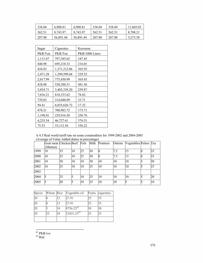
171

338.04 6,908.81 6,908.81 338.04 338.04 11,603.03

562.51 8,743.97 8,743.97 562.51 562.51 8,708.21

207.88 56,891.44 56,891.44 207.88 207.88 5,273.58

Sugar Cigarettes Kerosene

PKR/Ton PKR/Ton PKR/1000 Liters

1,113.47 797,385.62 187.45

840.98 695,218.33 216.01

434.93 1,371,312.06 365.93

2,471.28 1,299,599.68 229.52

2,017.99 775,450.99 365.43

428.08 520,388.51 481.56

3,034.71 3,403,338.20 259.87

7,016.21 818,333.62 78.82

739.03 314,048.09 33.71

94.41 6,035,626.72 17.32

478.21 700,983.72 173.71

1,198.01 229,916.50 258.76

4,235.54 46,727.61 376.51

75.53 33,112.56 356.22

A 4.5 Real world tariff rate on some commodities for 1999-2002 and 2004-2005 (Average of Value Added duties in percentage)

Goat meat (Mutton)

Chicken Beef Fish Milk Potatoes Onions Vegetables Pulses Tea

1999 10 35 10 25 30 0 7.5 15 0 35

2000 10 35 10 25 30 0 7.5 15 0 35

2001 10 30 10 10 30 10 10 10 5 30

2002 10 25 10 10 25 10 10 10 5 25

2003

2004 5 25 5 10 25 10 10 10 5 20

2005 5 20 5 10 25 10 10 5 5 10

Spices Wheat Rice Vegetable oil Fruits cigarettes

20 0 15 27.91 25 35

20 0 15 27.91 25 35

20 5 10 9756.2582 30 30

20 25 10 12431.2583 25 25

82 PKR/ton 83 Ibid

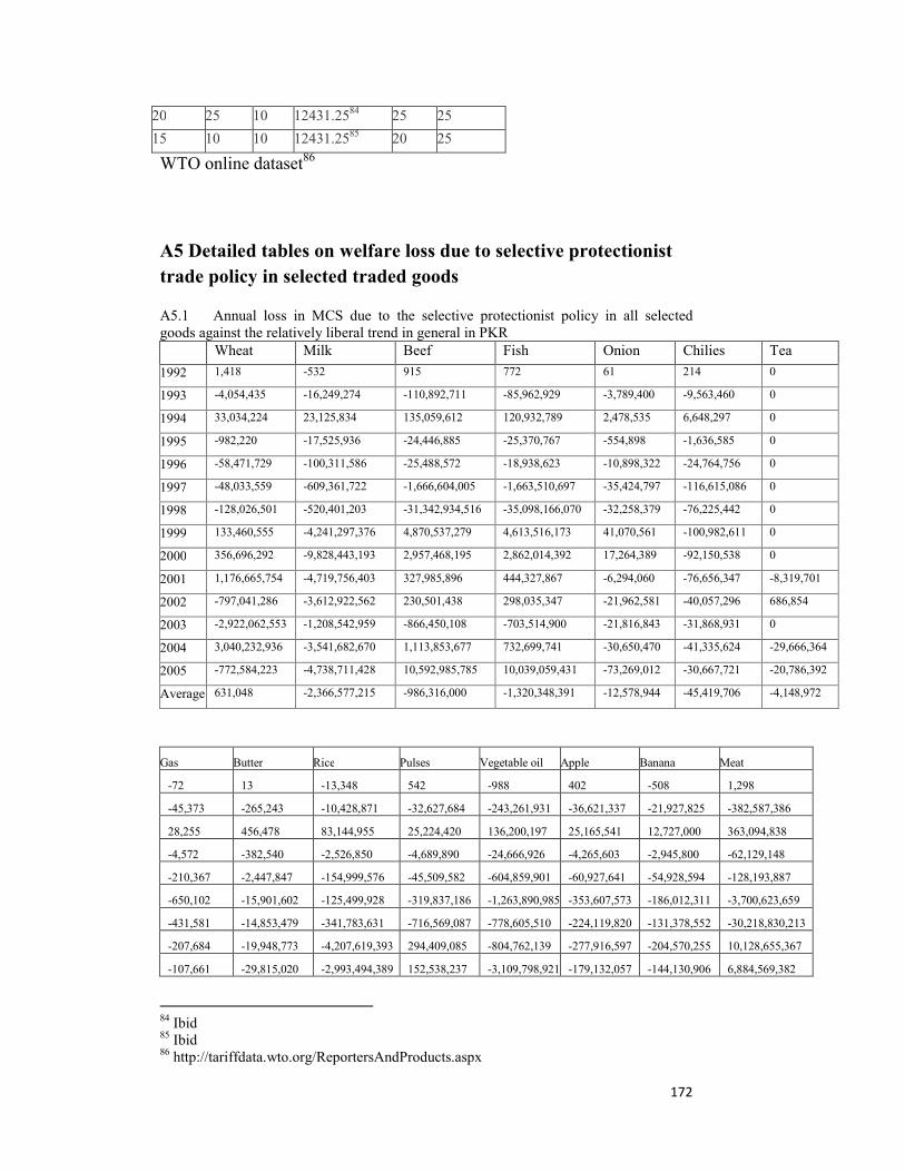
172

20 25 10 12431.2584 25 25

15 10 10 12431.2585 20 25

WTO online dataset86

A5 Detailed tables on welfare loss due to selective protectionist trade policy in selected traded goods A5.1 Annual loss in MCS due to the selective protectionist policy in all selected goods against the relatively liberal trend in general in PKR Wheat Milk Beef Fish Onion Chilies Tea 1992 1,418 -532 915 772 61 214 0

1993 -4,054,435 -16,249,274 -110,892,711 -85,962,929 -3,789,400 -9,563,460 0

1994 33,034,224 23,125,834 135,059,612 120,932,789 2,478,535 6,648,297 0

1995 -982,220 -17,525,936 -24,446,885 -25,370,767 -554,898 -1,636,585 0

1996 -58,471,729 -100,311,586 -25,488,572 -18,938,623 -10,898,322 -24,764,756 0

1997 -48,033,559 -609,361,722 -1,666,604,005 -1,663,510,697 -35,424,797 -116,615,086 0

1998 -128,026,501 -520,401,203 -31,342,934,516 -35,098,166,070 -32,258,379 -76,225,442 0

1999 133,460,555 -4,241,297,376 4,870,537,279 4,613,516,173 41,070,561 -100,982,611 0

2000 356,696,292 -9,828,443,193 2,957,468,195 2,862,014,392 17,264,389 -92,150,538 0

2001 1,176,665,754 -4,719,756,403 327,985,896 444,327,867 -6,294,060 -76,656,347 -8,319,701

2002 -797,041,286 -3,612,922,562 230,501,438 298,035,347 -21,962,581 -40,057,296 686,854

2003 -2,922,062,553 -1,208,542,959 -866,450,108 -703,514,900 -21,816,843 -31,868,931 0

2004 3,040,232,936 -3,541,682,670 1,113,853,677 732,699,741 -30,650,470 -41,335,624 -29,666,364

2005 -772,584,223 -4,738,711,428 10,592,985,785 10,039,059,431 -73,269,012 -30,667,721 -20,786,392

Average 631,048 -2,366,577,215 -986,316,000 -1,320,348,391 -12,578,944 -45,419,706 -4,148,972

Gas Butter Rice Pulses Vegetable oil Apple Banana Meat

-72 13 -13,348 542 -988 402 -508 1,298

-45,373 -265,243 -10,428,871 -32,627,684 -243,261,931 -36,621,337 -21,927,825 -382,587,386

28,255 456,478 83,144,955 25,224,420 136,200,197 25,165,541 12,727,000 363,094,838

-4,572 -382,540 -2,526,850 -4,689,890 -24,666,926 -4,265,603 -2,945,800 -62,129,148

-210,367 -2,447,847 -154,999,576 -45,509,582 -604,859,901 -60,927,641 -54,928,594 -128,193,887

-650,102 -15,901,602 -125,499,928 -319,837,186 -1,263,890,985 -353,607,573 -186,012,311 -3,700,623,659

-431,581 -14,853,479 -341,783,631 -716,569,087 -778,605,510 -224,119,820 -131,378,552 -30,218,830,213

-207,684 -19,948,773 -4,207,619,393 294,409,085 -804,762,139 -277,916,597 -204,570,255 10,128,655,367

-107,661 -29,815,020 -2,993,494,389 152,538,237 -3,109,798,921 -179,132,057 -144,130,906 6,884,569,382

84 Ibid 85 Ibid 86 http://tariffdata.wto.org/ReportersAndProducts.aspx

173

-123,483 -81,552,355 1,789,266,185 -5,491,263 -3,360,095,773 -147,384,536 -195,982,464 13,964,877

-813,308 -108,200,647 373,358,626 -17,865,422 -4,424,034,042 -81,707,351 -110,882,068 -1,671,107,685

-1,056,816 -64,543,757 -8,238,068,996 -45,958,512 -2,272,364,723 -79,830,818 -69,414,475 -2,269,069,938

-1,170,737 -102,894,092 12,216,560,620 34,006,172 -4,053,783,313 -113,936,526 -79,683,230 917,787,194

-2,076,229 -191,686,349 -4,775,592,194 -96,113,173 -3,815,467,911 -83,246,041 -49,576,392 24,045,345,600

-490,695 -45,145,372 -456,264,056 -55,605,953 -1,758,528,062 -115,537,854 -88,479,027 280,062,617

Chicken Potato Other

vegetables Other spices Sugar Cigarettes Firewood Kerosene Electricity

1,334 2,864 0 91 -6,450 0 0 70 0

-82,757,920 -153,687,573 -205,793,218 -37,942,451 -139,631,471 0 -1,606 -1,591,067 1

138,702,904 99,085,264 65,784,150 21,910,752 24,490,319 0 1,337 1,000,737 0

-31,042,591 -22,252,274 -19,103,734 -4,753,318 -42,833,463 0 -269 -154,737 0

0 -414,477,501 -360,380,110 -114,386,226 -951,678,179 0 -6,057 -7,417,040 2

-1,813,528,590 -1,978,663,468 -1,513,873,415 -277,147,796 -401,624,716 0 -17,228 -23,316,895 5

-50,267,045,591 -1,016,752,385 0 -264,726,404 -4,058,760,747 0 -2,608 -16,060,388 3

4,201,487,968 2,356,106,165 684,445,874 346,172,625 -14,707,551,058 0 -10,302 -7,730,273 2

1,061,304,377 1,465,081,113 29,528,376 106,773,429 -1,390,577,654 0 -25,184 -4,191,854 1

-49,773,108 276,161,508 -304,439,589 251,233,438 -370,576,674 0 -14,513 -5,009,564 7

-197,617,755 185,988,231 -143,848,292 433,098,064 -1,291,936,061 0 -21,415 -29,903,128 7

-699,545,805 -728,559,990 -385,059,738 -370,933,129 -2,618,876,802 0 -18,013 -41,575,586 0

-848,419,959 585,865,214 -160,326,914 103,773,153 -8,163,013,548 0 8,336 -45,033,171 5

5,966,026,953 -1,054,639,851 -1,791,403,638 -89,448,893 -237,644,908 0 -55,504 -80,000,325 1

-3,044,443,413 -28,624,477 -293,176,446 7,401,667 -2,453,587,244 0 -11,645 -18,641,659 2

A 5.2 Annual loss in HCV due to selective protectionist policy in all selected goods against the relatively liberal trend in general in PKR Wheat Milk Beef Fish Onion Chilies Tea 1992 1,403 -512 857 193 0 176 0

1993 -4,006,456 -15,673,817 -85,759,158 0 -130,478 -7,383,665 0

1994 32,577,915 21,923,662 111,957,919 0 0 5,158,588 0

1995 -967,353 -16,748,536 -20,007,773 -2,867,620 0 -1,294,019 0

1996 -57,483,468 -95,655,213 -14,111,876 0 -46,623 -18,280,007 0

1997 -47,164,207 -579,045,214 -1,343,367,620 -117,856,609 0 -90,395,468 0

1998 -125,556,732 -492,364,662 -29,466,853,106 -14,754,671,473 0 -57,408,426 0

1999 130,262,036 -3,962,948,484 3,647,219,846 435,488,774 0 -68,928,954 0

2000 347,481,319 -8,979,766,000 1,988,544,336 0 0 -69,024,817 0

2001 1,144,409,651 -4,366,686,826 182,525,203 0 0 -46,802,002 0

2002 -773,108,459 -3,318,759,712 136,321,061 0 0 -22,292,383 0

2003 -2,823,533,689 -1,083,732,861 -563,572,140 0 0 -19,192,246 0

2004 2,925,130,279 -3,190,385,090 733,497,778 0 0 -25,179,952 0

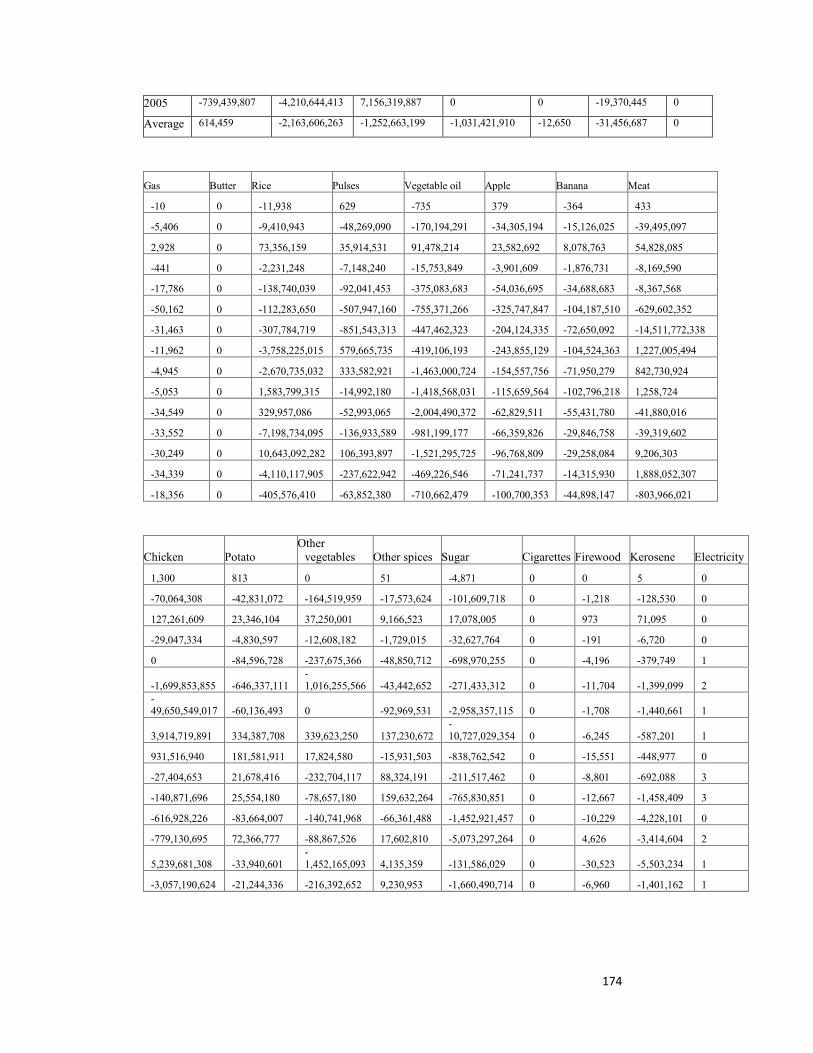
174

2005 -739,439,807 -4,210,644,413 7,156,319,887 0 0 -19,370,445 0

Average 614,459 -2,163,606,263 -1,252,663,199 -1,031,421,910 -12,650 -31,456,687 0

Gas Butter Rice Pulses Vegetable oil Apple Banana Meat

-10 0 -11,938 629 -735 379 -364 433

-5,406 0 -9,410,943 -48,269,090 -170,194,291 -34,305,194 -15,126,025 -39,495,097

2,928 0 73,356,159 35,914,531 91,478,214 23,582,692 8,078,763 54,828,085

-441 0 -2,231,248 -7,148,240 -15,753,849 -3,901,609 -1,876,731 -8,169,590

-17,786 0 -138,740,039 -92,041,453 -375,083,683 -54,036,695 -34,688,683 -8,367,568

-50,162 0 -112,283,650 -507,947,160 -755,371,266 -325,747,847 -104,187,510 -629,602,352

-31,463 0 -307,784,719 -851,543,313 -447,462,323 -204,124,335 -72,650,092 -14,511,772,338

-11,962 0 -3,758,225,015 579,665,735 -419,106,193 -243,855,129 -104,524,363 1,227,005,494

-4,945 0 -2,670,735,032 333,582,921 -1,463,000,724 -154,557,756 -71,950,279 842,730,924

-5,053 0 1,583,799,315 -14,992,180 -1,418,568,031 -115,659,564 -102,796,218 1,258,724

-34,549 0 329,957,086 -52,993,065 -2,004,490,372 -62,829,511 -55,431,780 -41,880,016

-33,552 0 -7,198,734,095 -136,933,589 -981,199,177 -66,359,826 -29,846,758 -39,319,602

-30,249 0 10,643,092,282 106,393,897 -1,521,295,725 -96,768,809 -29,258,084 9,206,303

-34,339 0 -4,110,117,905 -237,622,942 -469,226,546 -71,241,737 -14,315,930 1,888,052,307

-18,356 0 -405,576,410 -63,852,380 -710,662,479 -100,700,353 -44,898,147 -803,966,021

Chicken Potato Other

vegetables Other spices Sugar Cigarettes Firewood Kerosene Electricity

1,300 813 0 51 -4,871 0 0 5 0

-70,064,308 -42,831,072 -164,519,959 -17,573,624 -101,609,718 0 -1,218 -128,530 0

127,261,609 23,346,104 37,250,001 9,166,523 17,078,005 0 973 71,095 0

-29,047,334 -4,830,597 -12,608,182 -1,729,015 -32,627,764 0 -191 -6,720 0

0 -84,596,728 -237,675,366 -48,850,712 -698,970,255 0 -4,196 -379,749 1

-1,699,853,855 -646,337,111 -1,016,255,566 -43,442,652 -271,433,312 0 -11,704 -1,399,099 2

-49,650,549,017 -60,136,493 0 -92,969,531 -2,958,357,115 0 -1,708 -1,440,661 1

3,914,719,891 334,387,708 339,623,250 137,230,672 -10,727,029,354 0 -6,245 -587,201 1

931,516,940 181,581,911 17,824,580 -15,931,503 -838,762,542 0 -15,551 -448,977 0

-27,404,653 21,678,416 -232,704,117 88,324,191 -211,517,462 0 -8,801 -692,088 3

-140,871,696 25,554,180 -78,657,180 159,632,264 -765,830,851 0 -12,667 -1,458,409 3

-616,928,226 -83,664,007 -140,741,968 -66,361,488 -1,452,921,457 0 -10,229 -4,228,101 0

-779,130,695 72,366,777 -88,867,526 17,602,810 -5,073,297,264 0 4,626 -3,414,604 2

5,239,681,308 -33,940,601 -1,452,165,093 4,135,359 -131,586,029 0 -30,523 -5,503,234 1

-3,057,190,624 -21,244,336 -216,392,652 9,230,953 -1,660,490,714 0 -6,960 -1,401,162 1

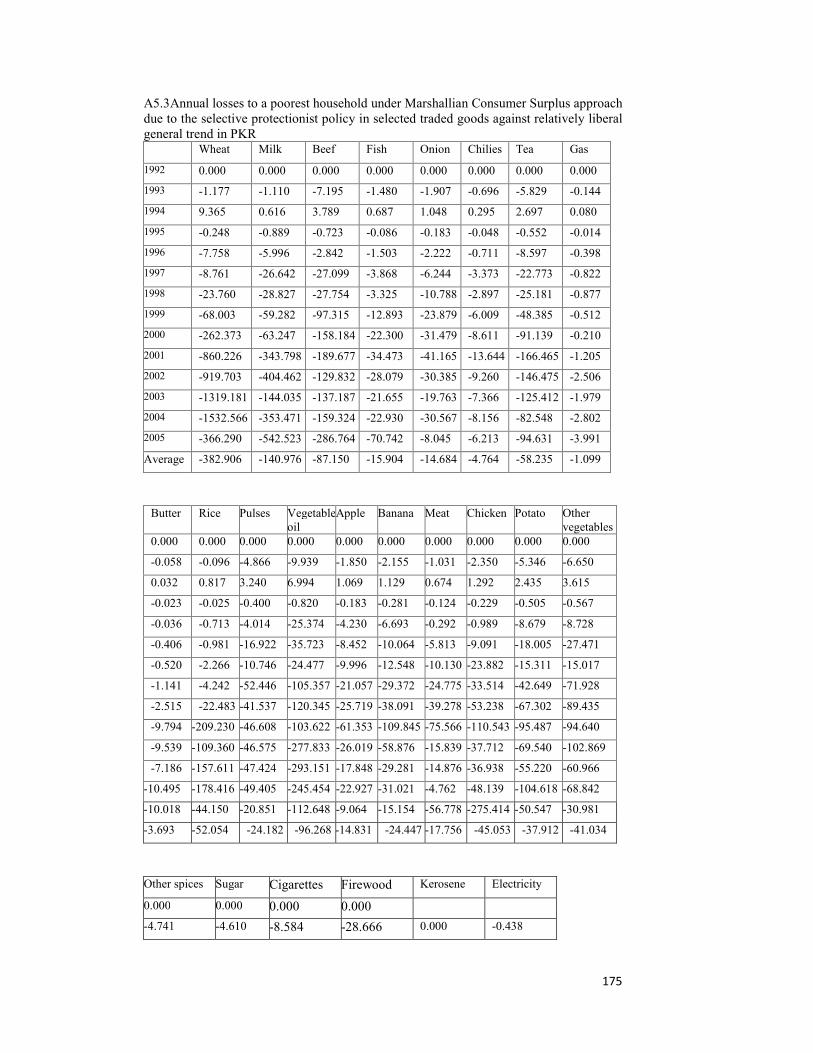
175

A5.3Annual losses to a poorest household under Marshallian Consumer Surplus approach due to the selective protectionist policy in selected traded goods against relatively liberal general trend in PKR Wheat Milk Beef Fish Onion Chilies Tea Gas

1992 0.000 0.000 0.000 0.000 0.000 0.000 0.000 0.000

1993 -1.177 -1.110 -7.195 -1.480 -1.907 -0.696 -5.829 -0.144

1994 9.365 0.616 3.789 0.687 1.048 0.295 2.697 0.080

1995 -0.248 -0.889 -0.723 -0.086 -0.183 -0.048 -0.552 -0.014

1996 -7.758 -5.996 -2.842 -1.503 -2.222 -0.711 -8.597 -0.398

1997 -8.761 -26.642 -27.099 -3.868 -6.244 -3.373 -22.773 -0.822

1998 -23.760 -28.827 -27.754 -3.325 -10.788 -2.897 -25.181 -0.877

1999 -68.003 -59.282 -97.315 -12.893 -23.879 -6.009 -48.385 -0.512

2000 -262.373 -63.247 -158.184 -22.300 -31.479 -8.611 -91.139 -0.210

2001 -860.226 -343.798 -189.677 -34.473 -41.165 -13.644 -166.465 -1.205

2002 -919.703 -404.462 -129.832 -28.079 -30.385 -9.260 -146.475 -2.506

2003 -1319.181 -144.035 -137.187 -21.655 -19.763 -7.366 -125.412 -1.979

2004 -1532.566 -353.471 -159.324 -22.930 -30.567 -8.156 -82.548 -2.802

2005 -366.290 -542.523 -286.764 -70.742 -8.045 -6.213 -94.631 -3.991

Average -382.906 -140.976 -87.150 -15.904 -14.684 -4.764 -58.235 -1.099

Butter Rice Pulses Vegetable oil

Apple Banana Meat Chicken Potato Other vegetables

0.000 0.000 0.000 0.000 0.000 0.000 0.000 0.000 0.000 0.000

-0.058 -0.096 -4.866 -9.939 -1.850 -2.155 -1.031 -2.350 -5.346 -6.650

0.032 0.817 3.240 6.994 1.069 1.129 0.674 1.292 2.435 3.615

-0.023 -0.025 -0.400 -0.820 -0.183 -0.281 -0.124 -0.229 -0.505 -0.567

-0.036 -0.713 -4.014 -25.374 -4.230 -6.693 -0.292 -0.989 -8.679 -8.728

-0.406 -0.981 -16.922 -35.723 -8.452 -10.064 -5.813 -9.091 -18.005 -27.471

-0.520 -2.266 -10.746 -24.477 -9.996 -12.548 -10.130 -23.882 -15.311 -15.017

-1.141 -4.242 -52.446 -105.357 -21.057 -29.372 -24.775 -33.514 -42.649 -71.928

-2.515 -22.483 -41.537 -120.345 -25.719 -38.091 -39.278 -53.238 -67.302 -89.435

-9.794 -209.230 -46.608 -103.622 -61.353 -109.845 -75.566 -110.543 -95.487 -94.640

-9.539 -109.360 -46.575 -277.833 -26.019 -58.876 -15.839 -37.712 -69.540 -102.869

-7.186 -157.611 -47.424 -293.151 -17.848 -29.281 -14.876 -36.938 -55.220 -60.966

-10.495 -178.416 -49.405 -245.454 -22.927 -31.021 -4.762 -48.139 -104.618 -68.842

-10.018 -44.150 -20.851 -112.648 -9.064 -15.154 -56.778 -275.414 -50.547 -30.981

-3.693 -52.054 -24.182 -96.268 -14.831 -24.447 -17.756 -45.053 -37.912 -41.034

Other spices Sugar Cigarettes Firewood Kerosene Electricity

0.000 0.000 0.000 0.000

-4.741 -4.610 -8.584 -28.666 0.000 -0.438

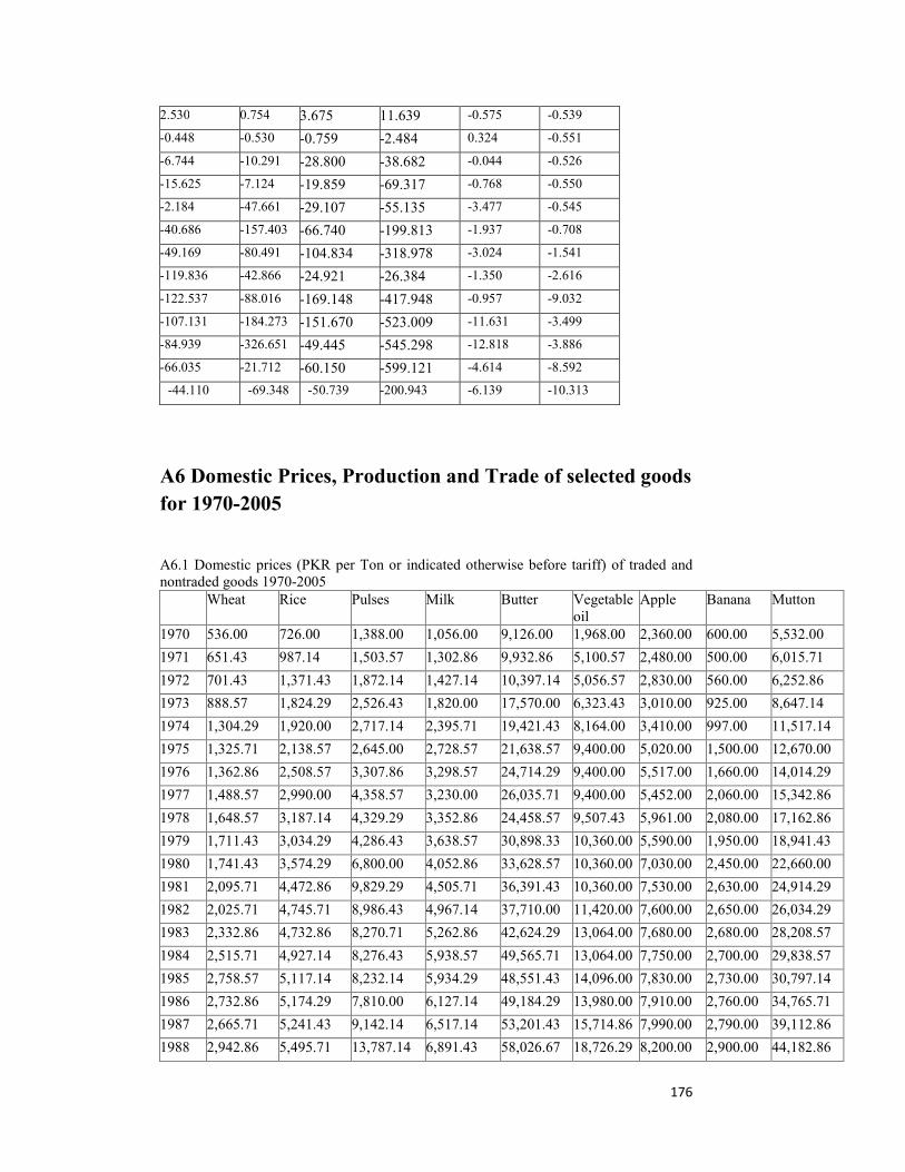
176

2.530 0.754 3.675 11.639 -0.575 -0.539

-0.448 -0.530 -0.759 -2.484 0.324 -0.551

-6.744 -10.291 -28.800 -38.682 -0.044 -0.526

-15.625 -7.124 -19.859 -69.317 -0.768 -0.550

-2.184 -47.661 -29.107 -55.135 -3.477 -0.545

-40.686 -157.403 -66.740 -199.813 -1.937 -0.708

-49.169 -80.491 -104.834 -318.978 -3.024 -1.541

-119.836 -42.866 -24.921 -26.384 -1.350 -2.616

-122.537 -88.016 -169.148 -417.948 -0.957 -9.032

-107.131 -184.273 -151.670 -523.009 -11.631 -3.499

-84.939 -326.651 -49.445 -545.298 -12.818 -3.886

-66.035 -21.712 -60.150 -599.121 -4.614 -8.592

-44.110 -69.348 -50.739 -200.943 -6.139 -10.313

A6 Domestic Prices, Production and Trade of selected goods for 1970-2005

A6.1 Domestic prices (PKR per Ton or indicated otherwise before tariff) of traded and nontraded goods 1970-2005 Wheat Rice Pulses Milk Butter Vegetable

oil Apple Banana Mutton

1970 536.00 726.00 1,388.00 1,056.00 9,126.00 1,968.00 2,360.00 600.00 5,532.00

1971 651.43 987.14 1,503.57 1,302.86 9,932.86 5,100.57 2,480.00 500.00 6,015.71

1972 701.43 1,371.43 1,872.14 1,427.14 10,397.14 5,056.57 2,830.00 560.00 6,252.86

1973 888.57 1,824.29 2,526.43 1,820.00 17,570.00 6,323.43 3,010.00 925.00 8,647.14

1974 1,304.29 1,920.00 2,717.14 2,395.71 19,421.43 8,164.00 3,410.00 997.00 11,517.14

1975 1,325.71 2,138.57 2,645.00 2,728.57 21,638.57 9,400.00 5,020.00 1,500.00 12,670.00

1976 1,362.86 2,508.57 3,307.86 3,298.57 24,714.29 9,400.00 5,517.00 1,660.00 14,014.29

1977 1,488.57 2,990.00 4,358.57 3,230.00 26,035.71 9,400.00 5,452.00 2,060.00 15,342.86

1978 1,648.57 3,187.14 4,329.29 3,352.86 24,458.57 9,507.43 5,961.00 2,080.00 17,162.86

1979 1,711.43 3,034.29 4,286.43 3,638.57 30,898.33 10,360.00 5,590.00 1,950.00 18,941.43

1980 1,741.43 3,574.29 6,800.00 4,052.86 33,628.57 10,360.00 7,030.00 2,450.00 22,660.00

1981 2,095.71 4,472.86 9,829.29 4,505.71 36,391.43 10,360.00 7,530.00 2,630.00 24,914.29

1982 2,025.71 4,745.71 8,986.43 4,967.14 37,710.00 11,420.00 7,600.00 2,650.00 26,034.29

1983 2,332.86 4,732.86 8,270.71 5,262.86 42,624.29 13,064.00 7,680.00 2,680.00 28,208.57

1984 2,515.71 4,927.14 8,276.43 5,938.57 49,565.71 13,064.00 7,750.00 2,700.00 29,838.57

1985 2,758.57 5,117.14 8,232.14 5,934.29 48,551.43 14,096.00 7,830.00 2,730.00 30,797.14

1986 2,732.86 5,174.29 7,810.00 6,127.14 49,184.29 13,980.00 7,910.00 2,760.00 34,765.71

1987 2,665.71 5,241.43 9,142.14 6,517.14 53,201.43 15,714.86 7,990.00 2,790.00 39,112.86

1988 2,942.86 5,495.71 13,787.14 6,891.43 58,026.67 18,726.29 8,200.00 2,900.00 44,182.86

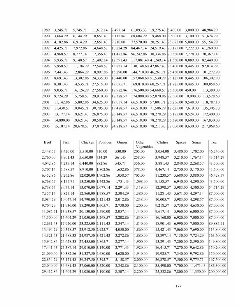
177

1989 3,245.71 5,745.71 11,612.14 7,497.14 61,093.33 19,275.43 8,400.00 3,000.00 48,984.29

1990 3,664.29 6,144.29 10,651.43 8,112.86 68,604.29 19,468.00 8,500.00 3,100.00 51,624.29

1991 4,182.86 6,914.29 12,651.43 9,210.00 77,570.00 20,251.43 23,675.00 5,000.00 55,154.29

1992 4,425.71 7,972.86 14,648.57 10,224.29 84,467.14 24,519.43 20,175.00 7,222.00 61,260.00

1993 4,968.57 8,777.14 17,356.43 11,482.86 96,242.86 30,334.86 20,350.00 7,778.00 70,367.14

1994 5,935.71 9,148.57 21,402.14 12,591.43 117,881.40 41,249.14 21,350.00 8,889.00 82,440.00

1995 5,958.57 11,194.29 22,548.57 13,827.14 130,148.60 42,867.43 23,400.00 9,445.00 92,814.29

1996 7,441.43 12,864.29 18,997.86 15,290.00 144,710.00 46,261.71 25,450.00 8,889.00 101,272.90

1997 8,691.43 13,302.86 24,335.00 16,440.00 157,068.60 51,530.29 25,125.00 9,445.00 106,302.90

1998 8,381.43 14,535.71 27,515.00 17,675.71 169,810.00 60,257.71 21,725.00 9,445.00 109,858.60

1999 9,035.71 16,124.29 27,560.00 17,982.86 176,500.00 54,668.57 25,300.00 450.00 113,380.00

2000 9,724.29 15,758.57 29,910.00 18,388.57 174,880.00 52,070.86 27,500.00 10,000.00 113,528.60

2001 11,142.86 15,802.86 34,625.00 19,057.14 66,518.00 57,801.71 26,256.00 9,548.00 118,787.10

2002 11,438.57 18,045.71 30,795.00 19,488.57 66,518.00 71,586.29 18,625.00 7,619.00 135,305.70

2003 13,177.14 19,621.43 26,075.00 20,148.57 66,518.00 78,278.29 36,175.00 9,524.00 172,400.00

2004 14,890.00 19,621.43 30,505.00 20,148.57 66,518.00 78,278.29 36,380.00 9,600.00 167,830.00

2005 15,107.14 20,678.57 37,070.00 24,818.57 66,518.00 78,211.43 37,000.00 9,630.00 217,968.60

Beef Fish Chicken Potatoes Onion Other Vegetables

Chilies Spices Sugar Tea

2,448.57 3,420.00 5,510.00 710.00 530.00 205.00 3,054.00 3,480.00 1,702.00 46,240.00

2,760.00 3,901.43 5,650.00 734.29 561.43 258.00 3,948.57 3,210.00 1,767.14 43,514.29

4,042.86 4,237.14 6,440.00 882.86 545.71 356.00 3,881.43 2,840.00 2,268.57 43,500.00

5,707.14 5,588.57 8,910.00 1,802.86 1,632.86 378.00 4,467.14 2,750.00 3,170.00 43,500.00

6,452.86 7,262.86 12,020.00 1,702.86 1,058.57 705.00 11,238.57 5,680.00 3,880.00 46,428.57

6,768.57 8,175.71 13,250.00 1,442.86 1,731.43 1,098.00 9,158.57 6,940.00 4,290.00 43,500.00

6,738.57 9,077.14 13,070.00 2,077.14 2,291.43 1,119.00 12,398.57 5,983.00 4,300.00 54,714.29

7,357.14 9,827.14 12,860.00 1,988.57 2,304.29 1,380.00 11,281.43 5,671.00 4,297.14 87,000.00

8,084.29 10,047.14 14,790.00 2,121.43 2,012.86 1,238.00 10,005.71 5,983.00 4,298.57 87,000.00

9,704.29 11,930.00 18,290.00 1,605.71 2,730.00 1,200.00 9,218.57 5,750.00 4,630.00 87,000.00

11,085.71 13,938.57 20,130.00 2,590.00 2,057.14 1,440.00 9,617.14 5,960.00 6,000.00 87,000.00

11,500.00 15,604.29 21,050.00 3,268.57 3,202.86 1,830.00 16,160.00 6,920.00 7,000.00 87,000.00

12,631.43 17,920.00 23,225.00 2,111.43 2,347.14 1,840.00 18,901.43 6,990.00 7,000.00 89,885.71

13,494.29 20,348.57 23,912.50 2,925.71 4,050.00 1,860.00 15,421.43 7,060.00 7,690.00 113,800.00

14,321.43 21,688.33 24,987.50 3,421.43 3,272.86 1,880.00 13,897.14 7,130.00 7,724.29 163,600.00

15,942.86 24,628.33 27,455.00 2,865.71 2,277.14 1,900.00 13,291.43 7,200.00 8,590.00 149,800.00

17,441.43 25,387.14 29,010.00 3,140.00 3,771.43 1,920.00 16,415.71 7,270.00 9,642.86 150,200.00

21,090.00 30,382.86 31,327.50 4,680.00 4,620.00 1,940.00 19,925.71 7,340.00 9,792.86 150,000.00

22,834.29 33,171.43 36,247.50 5,395.71 5,158.57 2,000.00 36,878.57 7,500.00 9,775.71 167,500.00

25,040.00 34,681.43 37,060.00 3,520.00 3,342.86 2,100.00 35,490.00 7,700.00 11,471.43 186,300.00

29,412.86 41,604.29 41,080.00 5,190.00 8,307.14 2,200.00 25,332.86 7,800.00 11,350.00 200,000.00

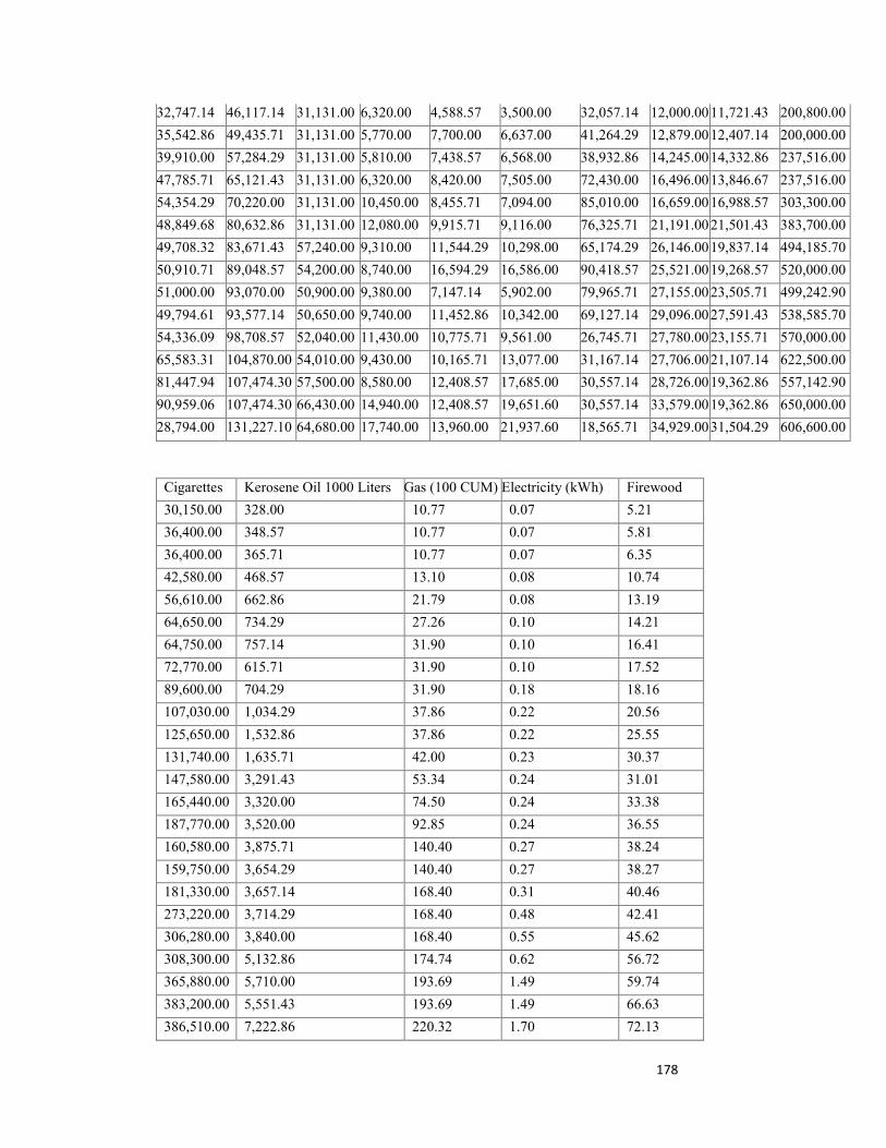
178

32,747.14 46,117.14 31,131.00 6,320.00 4,588.57 3,500.00 32,057.14 12,000.00 11,721.43 200,800.00

35,542.86 49,435.71 31,131.00 5,770.00 7,700.00 6,637.00 41,264.29 12,879.00 12,407.14 200,000.00

39,910.00 57,284.29 31,131.00 5,810.00 7,438.57 6,568.00 38,932.86 14,245.00 14,332.86 237,516.00

47,785.71 65,121.43 31,131.00 6,320.00 8,420.00 7,505.00 72,430.00 16,496.00 13,846.67 237,516.00

54,354.29 70,220.00 31,131.00 10,450.00 8,455.71 7,094.00 85,010.00 16,659.00 16,988.57 303,300.00

48,849.68 80,632.86 31,131.00 12,080.00 9,915.71 9,116.00 76,325.71 21,191.00 21,501.43 383,700.00

49,708.32 83,671.43 57,240.00 9,310.00 11,544.29 10,298.00 65,174.29 26,146.00 19,837.14 494,185.70

50,910.71 89,048.57 54,200.00 8,740.00 16,594.29 16,586.00 90,418.57 25,521.00 19,268.57 520,000.00

51,000.00 93,070.00 50,900.00 9,380.00 7,147.14 5,902.00 79,965.71 27,155.00 23,505.71 499,242.90

49,794.61 93,577.14 50,650.00 9,740.00 11,452.86 10,342.00 69,127.14 29,096.00 27,591.43 538,585.70

54,336.09 98,708.57 52,040.00 11,430.00 10,775.71 9,561.00 26,745.71 27,780.00 23,155.71 570,000.00

65,583.31 104,870.00 54,010.00 9,430.00 10,165.71 13,077.00 31,167.14 27,706.00 21,107.14 622,500.00

81,447.94 107,474.30 57,500.00 8,580.00 12,408.57 17,685.00 30,557.14 28,726.00 19,362.86 557,142.90

90,959.06 107,474.30 66,430.00 14,940.00 12,408.57 19,651.60 30,557.14 33,579.00 19,362.86 650,000.00

28,794.00 131,227.10 64,680.00 17,740.00 13,960.00 21,937.60 18,565.71 34,929.00 31,504.29 606,600.00

Cigarettes Kerosene Oil 1000 Liters Gas (100 CUM) Electricity (kWh) Firewood

30,150.00 328.00 10.77 0.07 5.21

36,400.00 348.57 10.77 0.07 5.81

36,400.00 365.71 10.77 0.07 6.35

42,580.00 468.57 13.10 0.08 10.74

56,610.00 662.86 21.79 0.08 13.19

64,650.00 734.29 27.26 0.10 14.21

64,750.00 757.14 31.90 0.10 16.41

72,770.00 615.71 31.90 0.10 17.52

89,600.00 704.29 31.90 0.18 18.16

107,030.00 1,034.29 37.86 0.22 20.56

125,650.00 1,532.86 37.86 0.22 25.55

131,740.00 1,635.71 42.00 0.23 30.37

147,580.00 3,291.43 53.34 0.24 31.01

165,440.00 3,320.00 74.50 0.24 33.38

187,770.00 3,520.00 92.85 0.24 36.55

160,580.00 3,875.71 140.40 0.27 38.24

159,750.00 3,654.29 140.40 0.27 38.27

181,330.00 3,657.14 168.40 0.31 40.46

273,220.00 3,714.29 168.40 0.48 42.41

306,280.00 3,840.00 168.40 0.55 45.62

308,300.00 5,132.86 174.74 0.62 56.72

365,880.00 5,710.00 193.69 1.49 59.74

383,200.00 5,551.43 193.69 1.49 66.63

386,510.00 7,222.86 220.32 1.70 72.13

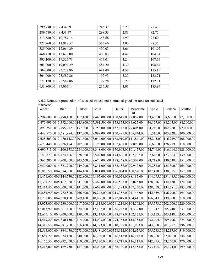
179

399,730.00 7,434.29 245.37 2.20 75.43

289,580.00 8,458.57 298.33 2.83 82.75

313,580.00 10,787.14 353.66 2.99 92.60

322,760.00 11,918.57 353.66 3.00 98.35

385,000.00 12,064.29 400.03 3.66 101.07

468,410.00 13,620.00 400.03 4.42 104.74

495,100.00 17,325.71 477.01 4.24 107.65

504,000.00 19,094.29 584.20 4.30 108.64

504,000.00 23,232.86 644.40 4.52 115.15

504,000.00 25,582.86 192.93 5.29 132.71

571,170.00 25,582.86 197.78 5.29 132.71

653,800.00 37,007.14 216.58 4.01 183.97

A 6.2 Domestic production of selected traded and nontraded goods in tons (or indicated otherwise)

Wheat Rice Pulses Milk Butter Vegetable Oil

Apple Banana Mutton

7,294,000.00 3,298,400.00 117,400.00 7,445,000.00 150,647.00 77,852.00 33,430.00 88,600.00 77,700.00

6,475,693.00 3,392,600.00 145,800.00 7,591,500.00 153,853.00 84,627.00 36,127.00 88,295.00 84,200.00

6,890,851.00 3,495,212.00 157,000.00 7,758,000.00 157,147.00 79,805.00 34,240.00 102,720.00 92,000.00

7,442,570.00 3,681,984.00 137,700.00 7,899,000.00 160,499.00 105,844.00 51,510.00 105,228.00 100,000.00

7,628,503.00 3,470,148.00 203,600.00 8,044,000.00 163,910.00 111,841.00 56,245.00 116,739.00 108,000.00

7,673,440.00 3,926,184.00 202,000.00 8,193,000.00 167,408.00 97,895.00 66,690.00 126,279.00 118,000.00

8,690,713.00 4,106,178.00 284,000.00 8,348,000.00 170,993.00 101,477.00 74,746.00 116,614.00 128,000.00

9,143,873.00 4,424,406.00 228,600.00 8,509,000.00 174,666.00 107,262.00 87,672.00 123,364.00 139,000.00

8,367,200.00 4,908,000.00 203,600.00 8,670,000.00 178,368.00 96,307.00 93,718.00 130,538.00 151,000.00

9,950,000.00 4,823,700.00 249,200.00 8,841,000.00 182,187.00 99,942.00 99,282.00 125,300.00 164,000.00

10,856,500.00 4,684,800.00 184,100.00 9,014,000.00 186,064.00 100,520.00 107,410.00 130,815.00 157,000.00

11,474,600.00 5,144,550.00 182,800.00 9,195,000.00 190,028.00 88,187.00 114,095.00 131,485.00 166,000.00

11,304,200.00 5,167,050.00 241,800.00 9,462,000.00 196,587.00 98,025.00 128,616.00 134,430.00 174,000.00

12,414,400.00 5,009,250.00 191,200.00 9,662,000.00 201,193.00 107,350.00 128,068.00 134,781.00 183,000.00

10,881,900.00 4,972,800.00 266,600.00 10,242,000.00 213,756.00 94,146.00 142,659.00 136,700.00 195,000.00

11,703,000.00 4,378,400.00 269,100.00 10,856,000.00 227,049.00 104,411.00 166,043.00 139,900.00 210,000.00

13,923,000.00 5,230,000.00 217,200.00 11,818,000.00 241,216.00 104,592.00 195,573.00 202,000.00 220,000.00

12,015,900.00 4,861,400.00 274,300.00 12,482,000.00 256,228.00 91,339.00 211,942.00 205,748.00 237,000.00

12,675,100.00 4,800,300.00 159,000.00 13,319,000.00 278,848.00 102,125.00 215,113.00 205,148.00 255,000.00

14,419,200.00 4,830,150.00 414,400.00 14,003,000.00 294,385.00 115,755.00 232,404.00 209,796.00 275,000.00

14,315,500.00 4,891,200.00 316,400.00 14,723,000.00 310,797.00 101,983.00 243,000.00 201,777.00 296,000.00

14,565,000.00 4,864,650.00 273,000.00 15,481,000.00 328,112.00 104,629.00 295,283.00 44,217.00 319,000.00

15,684,200.00 4,674,150.00 240,000.00 16,280,000.00 346,418.00 116,148.00 338,968.00 52,026.00 344,000.00

16,156,500.00 5,992,050.00 210,000.00 17,120,000.00 365,715.00 116,119.00 442,395.00 63,250.00 370,000.00

15,213,000.00 5,169,750.00 187,000.00 18,006,000.00 386,120.00 112,455.00 533,105.00 79,474.00 399,000.00

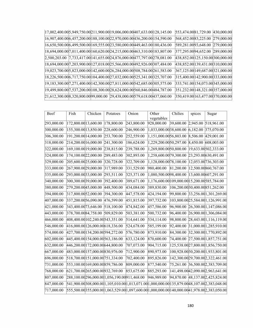
180

17,002,400.00 5,949,750.00 211,900.00 19,006,000.00 407,633.00 128,145.00 553,474.00 81,729.00 430,000.00

16,907,400.00 6,457,200.00 188,100.00 22,970,000.00 436,200.00 154,590.00 568,452.00 83,225.00 279,000.00

16,650,500.00 6,499,500.00 169,555.00 23,580,000.00 449,463.00 180,436.00 589,281.00 93,648.00 279,000.00

18,694,000.00 7,011,400.00 160,620.00 24,215,000.00 463,310.00 183,807.00 377,295.00 94,652.00 289,000.00

2,500,203.00 7,733,417.00 141,655.00 24,876,000.00 477,797.00 278,081.00 438,852.00 125,150.00 300,000.00

18,694,000.00 7,203,900.00 127,018.00 25,566,000.00 492,926.00 307,484.00 438,852.00 139,431.00 310,000.00

19,023,700.00 5,823,000.00 142,600.00 26,284,000.00 508,784.00 261,583.00 367,125.00 149,687.00 321,000.00

18,226,500.00 6,717,750.00 104,400.00 27,032,000.00 525,341.00 325,707.00 315,400.00 142,900.00 333,000.00

19,183,300.00 7,271,400.00 142,300.00 27,811,000.00 542,685.00 305,575.00 333,741.00 154,073.00 345,000.00

19,499,800.00 7,537,200.00 108,300.00 28,624,000.00 560,846.00 484,787.00 351,232.00 148,321.00 357,000.00

21,612,300.00 8,320,800.00 99,000.00 29,438,000.00 579,618.00 437,060.00 350,419.00 163,477.00 370,000.00

Beef Fish Chicken Potatoes Onion Other vegetables

Chilies spices Sugar

293,000.00 172,800.0013,600.00 178,800.00 243,800.00 928,000.00 39,600.00 2,945.00 518,961.00

300,000.00 155,300.0013,850.00 228,600.00 246,900.00 1,033,000.0038,600.00 6,182.00 375,070.00

306,300.00 191,200.0014,000.00 253,700.00 252,559.00 1,151,000.0056,803.00 8,506.00 429,001.00

318,000.00 214,200.0016,000.00 241,300.00 186,624.00 1,229,200.0050,297.00 8,450.00 608,003.00

322,000.00 169,100.0019,000.00 238,815.00 239,788.00 1,269,800.0050,800.00 19,633.00502,333.00

324,000.00 174,100.0022,000.00 289,483.00 302,893.00 1,258,600.0079,300.00 23,293.00630,491.00

329,000.00 205,600.0025,000.00 320,728.00 322,709.00 1,128,000.0078,100.00 12,053.00736,303.00

333,000.00 267,900.0029,000.00 317,989.00 331,529.00 980,400.00 81,200.00 12,500.00860,767.00

335,000.00 293,000.0033,000.00 293,511.00 325,371.00 1,080,500.0098,400.00 13,600.00607,291.00

340,000.00 300,300.0039,000.00 392,400.00 389,671.00 1,176,600.00109,000.0015,200.00585,784.00

380,000.00 279,200.0045,000.00 448,500.00 434,084.00 389,830.00 106,200.0030,400.00851,262.00

394,000.00 317,800.0052,000.00 394,300.00 447,578.00 424,194.00 99,800.00 33,256.001,301,269.00

407,000.00 337,200.0056,090.00 476,599.00 451,815.00 397,732.00 103,800.0025,584.001,126,991.00

421,000.00 343,400.0073,646.00 518,100.00 474,842.00 457,586.00 96,900.00 26,300.001,147,086.00

443,000.00 378,700.0084,758.00 509,829.00 503,381.00 500,732.00 96,400.00 26,900.001,306,084.00

466,000.00 408,400.00102,240.00543,351.00 514,641.00 534,114.00 98,800.00 28,443.001,116,119.00

546,000.00 416,000.00126,000.00618,336.00 524,678.00 585,199.00 92,400.00 31,000.001,285,910.00

574,000.00 427,700.00134,200.00594,272.00 576,780.00 873,910.00 84,300.00 32,300.001,770,892.00

602,000.00 445,400.00154,000.00563,186.00 633,124.00 870,600.00 74,400.00 27,500.001,857,751.00

632,000.00 446,200.00172,000.00644,800.00 707,073.00 904,715.00 125,538.0027,800.001,856,750.00

667,000.00 483,000.00157,000.00830,976.00 712,900.00 890,973.00 100,928.0030,200.001,933,801.00

696,000.00 518,700.00151,000.00751,334.00 702,400.00 895,826.00 142,300.0029,700.002,322,461.00

731,000.00 553,100.00169,000.00859,786.00 809,000.00 877,540.00 75,261.00 36,500.002,383,709.00

768,000.00 621,700.00265,000.00932,769.00 853,675.00 885,293.00 141,498.0042,090.002,963,641.00

807,000.00 288,100.00296,000.001,056,190.00911,468.00 946,989.00 94,870.00 48,137.002,425,824.00

847,000.00 541,900.00308,000.001,105,010.001,013,071.001,000,000.00135,879.0048,107.002,383,048.00

717,000.00 555,500.00355,000.001,063,529.001,097,600.001,000,000.00140,000.0041,978.002,383,050.00

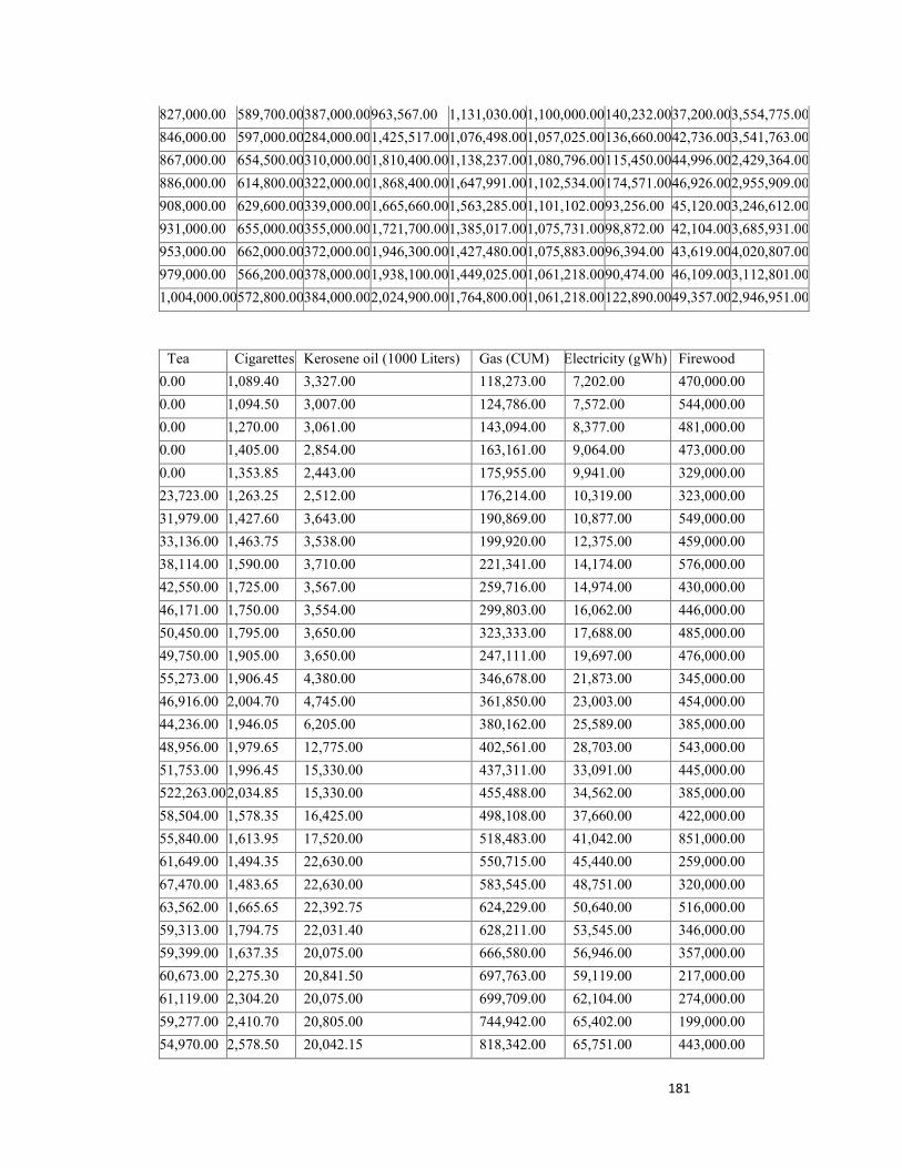
181

827,000.00 589,700.00387,000.00963,567.00 1,131,030.001,100,000.00140,232.0037,200.003,554,775.00

846,000.00 597,000.00284,000.001,425,517.001,076,498.001,057,025.00136,660.0042,736.003,541,763.00

867,000.00 654,500.00310,000.001,810,400.001,138,237.001,080,796.00115,450.0044,996.002,429,364.00

886,000.00 614,800.00322,000.001,868,400.001,647,991.001,102,534.00174,571.0046,926.002,955,909.00

908,000.00 629,600.00339,000.001,665,660.001,563,285.001,101,102.0093,256.00 45,120.003,246,612.00

931,000.00 655,000.00355,000.001,721,700.001,385,017.001,075,731.0098,872.00 42,104.003,685,931.00

953,000.00 662,000.00372,000.001,946,300.001,427,480.001,075,883.0096,394.00 43,619.004,020,807.00

979,000.00 566,200.00378,000.001,938,100.001,449,025.001,061,218.0090,474.00 46,109.003,112,801.00

1,004,000.00572,800.00384,000.002,024,900.001,764,800.001,061,218.00122,890.0049,357.002,946,951.00

Tea Cigarettes Kerosene oil (1000 Liters) Gas (CUM) Electricity (gWh) Firewood

0.00 1,089.40 3,327.00 118,273.00 7,202.00 470,000.00

0.00 1,094.50 3,007.00 124,786.00 7,572.00 544,000.00

0.00 1,270.00 3,061.00 143,094.00 8,377.00 481,000.00

0.00 1,405.00 2,854.00 163,161.00 9,064.00 473,000.00

0.00 1,353.85 2,443.00 175,955.00 9,941.00 329,000.00

23,723.00 1,263.25 2,512.00 176,214.00 10,319.00 323,000.00

31,979.00 1,427.60 3,643.00 190,869.00 10,877.00 549,000.00

33,136.00 1,463.75 3,538.00 199,920.00 12,375.00 459,000.00

38,114.00 1,590.00 3,710.00 221,341.00 14,174.00 576,000.00

42,550.00 1,725.00 3,567.00 259,716.00 14,974.00 430,000.00

46,171.00 1,750.00 3,554.00 299,803.00 16,062.00 446,000.00

50,450.00 1,795.00 3,650.00 323,333.00 17,688.00 485,000.00

49,750.00 1,905.00 3,650.00 247,111.00 19,697.00 476,000.00

55,273.00 1,906.45 4,380.00 346,678.00 21,873.00 345,000.00

46,916.00 2,004.70 4,745.00 361,850.00 23,003.00 454,000.00

44,236.00 1,946.05 6,205.00 380,162.00 25,589.00 385,000.00

48,956.00 1,979.65 12,775.00 402,561.00 28,703.00 543,000.00

51,753.00 1,996.45 15,330.00 437,311.00 33,091.00 445,000.00

522,263.00 2,034.85 15,330.00 455,488.00 34,562.00 385,000.00

58,504.00 1,578.35 16,425.00 498,108.00 37,660.00 422,000.00

55,840.00 1,613.95 17,520.00 518,483.00 41,042.00 851,000.00

61,649.00 1,494.35 22,630.00 550,715.00 45,440.00 259,000.00

67,470.00 1,483.65 22,630.00 583,545.00 48,751.00 320,000.00

63,562.00 1,665.65 22,392.75 624,229.00 50,640.00 516,000.00

59,313.00 1,794.75 22,031.40 628,211.00 53,545.00 346,000.00

59,399.00 1,637.35 20,075.00 666,580.00 56,946.00 357,000.00

60,673.00 2,275.30 20,841.50 697,763.00 59,119.00 217,000.00

61,119.00 2,304.20 20,075.00 699,709.00 62,104.00 274,000.00

59,277.00 2,410.70 20,805.00 744,942.00 65,402.00 199,000.00

54,970.00 2,578.50 20,042.15 818,342.00 65,751.00 443,000.00

182

46,367.00 2,424.45 19,345.00 857,433.00 52,717.00 543,000.00

54,783.00 2,903.75 19,863.30 923,758.00 72,406.00 478,000.00

57,685.00 3,004.00 21,852.55 992,589.00 75,682.00 444,000.00

59,269.00 3,104.50 23,458.55 1,202,750.00 80,826.00 505,000.00

60,501.00 3,154.50 21,900.00 1,344,953.00 85,629.00 752,000.00

59,197.00 2,970.55 22,630.00 1,400,025.00 94,030.00 478,000.00

A6.3 Import of selected traded goods in Tons (or indicated otherwise) Wheat Rice Pulses Milk Butter Vegetable

Oil Apple Banana Mutton Beef

228,600.00 20.00 6,600.00 40.00 40.00 40.00 800.00 0.00 0.00 10.00

286,571.00 20.00 1,300.00 15.00 51.00 36.00 904.00 0.00 0.00 2.00

704,800.00 60,096.00 117.00 30.00 25.00 73.00 682.00 0.00 0.00 1.00

1,359,505.00 10.00 100.00 30.00 586.00 95.00 1,000.00 0.00 0.00 2.00

1,228,630.00 0.00 0.00 158.00 17,820.00 0.00 2,554.00 0.00 1.00 0.00

1,344,147.00 20.00 0.00 15.00 1,803.00 0.00 1,485.00 0.00 0.00 1.00

1,185,588.00 12.00 0.00 187.00 7,933.00 0.00 1,318.00 0.00 0.00 1.00

497,500.00 0.00 0.00 17.00 1,812.00 0.00 1,200.00 0.00 0.00 0.00

1,051,559.00 15.00 0.00 0.00 7,566.00 0.00 905.00 5.00 0.00 17.00

2,236,489.00 1.00 614.00 97.00 3,296.00 169.00 1,530.00 0.00 0.00 1.00

602,208.00 3.00 1,055.00 474.00 4,827.00 3,500.00 1,148.00 0.00 2.00 0.00

304,820.00 0.00 105.00 8.00 3,287.00 921.00 4,071.00 0.00 51.00 0.00

359,808.00 3.00 31,310.00 23.00 2,086.00 2,623.00 3,112.00 0.00 0.00 0.00

396,008.00 15.00 2,354.00 601.00 287.00 592.00 4,217.00 0.00 0.00 0.00

290,775.00 4.00 5,448.00 161.00 6,800.00 610.00 5,029.00 0.00 0.00 0.00

979,998.00 7.00 2,637.00 20.00 1,978.00 4,772.00 3,153.00 6.00 0.00 0.00

1,909,198.00 0.00 11,138.00 0.00 503.00 8,467.00 2,669.00 0.00 0.00 1.00

377,788.00 0.00 24,192.00 0.00 3,235.00 333.00 3,405.00 0.00 0.00 2.00

600,867.00 1,265.00 8,828.00 0.00 5,008.00 9,637.00 4,189.00 0.00 0.00 0.00

2,170,798.00 0.00 4,972.00 0.00 1,567.00 989.00 2,020.00 0.00 0.00 0.00

2,047,418.00 25.00 23,706.00 943.00 1,659.00 6,483.00 409.00 0.00 0.00 0.00

972,073.00 1.00 8,554.00 24.00 8,178.00 5,535.00 1,560.00 0.00 0.00 0.00

2,018,165.00 41.00 23,309.00 3.00 8,478.00 2,811.00 2,536.00 0.00 0.00 0.00

2,890,196.00 322.00 60,352.00 0.00 24,762.00 2,020.00 2,217.00 0.00 0.00 0.00

1,901,646.00 220.00 30,435.00 111.00 2,079.00 18.00 2,327.00 0.00 0.00 0.00

2,616,581.00 39.00 44,121.00 0.00 229.00 1,270.00 8,324.00 6.00 91.00 2.00

1,968,110.00 1,390.00 23,182.00 0.00 172.00 4,922.00 5,783.00 92.00 173.00 0.00

2,500,203.00 200.00 32,364.00 96.00 143.00 1,831.00 5,537.00 47.00 0.00 0.00

2,520,071.00 853.00 40,832.00 52.00 486.00 240.00 3,003.00 0.00 0.00 1.00

3,239,759.00 1,471.00 31,740.00 9.00 334.00 973.00 3,882.00 0.00 0.00 1.00

1,048,180.00 718.00 26,368.00 171.00 208.00 75.00 7,436.00 0.00 6.00 0.00

149,121.00 10,542.00 31,342.00 0.00 176.00 47.00 3,040.00 0.00 0.00 0.00

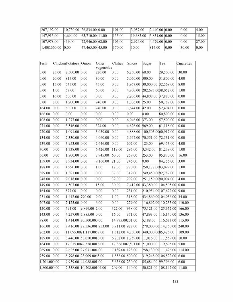
183

267,192.00 10,730.00 26,834.00 0.00 101.00 3,057.00 2,440.00 0.00 0.00 4.00

147,913.00 4,694.00 65,710.00 11.00 135.00 19,683.00 3,831.00 0.00 0.00 15.00

107,978.00 439.00 72,946.00 62.00 105.00 2,924.00 4,479.00 0.00 0.00 27.00

1,408,660.00 0.00 47,465.00 45.00 170.00 10.00 814.00 0.00 30.00 0.00

Fish Chicken Potatoes Onion Other vegetables

Chilies Spices Sugar Tea Cigarettes

0.00 25.00 2,500.00 0.00 220.00 0.00 6,250.00 68.00 29,500.00 30.00

0.00 20.00 817.00 0.00 30.00 0.00 5,050.00 300.00 31,800.00 4.00

0.00 15.00 545.00 0.00 45.00 0.00 1,967.00 30,000.00 32,568.00 8.00

0.00 1.00 57.00 0.00 60.00 0.00 4,800.00 202,683.0038,052.00 1.00

0.00 16.00 500.00 0.00 0.00 0.00 2,206.00 44,808.00 37,880.00 0.00

0.00 8.00 1,200.00 0.00 240.00 0.00 1,306.00 25.00 50,787.00 5.00

164.00 0.00 800.00 0.00 240.00 0.00 3,644.00 42.00 52,404.00 0.00

166.00 0.00 0.00 0.00 0.00 0.00 0.00 0.00 60,800.00 0.00

108.00 0.00 1,277.00 0.00 0.00 0.00 6,946.00 373.00 57,500.00 0.00

271.00 0.00 3,516.00 0.00 324.00 0.00 4,626.00 969.00 61,118.00 0.00

220.00 0.00 1,091.00 0.00 3,039.00 0.00 4,888.00 100,505.0060,912.00 0.00

134.00 0.00 2,330.00 0.00 4,060.00 0.00 5,667.00 70,551.00 72,531.00 0.00

239.00 0.00 3,953.00 0.00 2,646.00 0.00 602.00 123.00 69,453.00 4.00

70.00 0.00 1,738.00 0.00 6,426.00 119.00 295.00 3,342.00 81,239.00 1.00

66.00 0.00 1,800.00 0.00 7,945.00 60.00 259.00 253.00 95,870.00 16.00

159.00 0.00 3,934.00 0.00 9,160.00 21.00 246.00 0.00 84,256.00 3.00

188.00 0.00 4,990.00 0.00 1.00 12.00 270.00 258,177.0083,099.00 1.00

389.00 0.00 1,381.00 0.00 0.00 37.00 319.00 749,450.0092,787.00 1.00

248.00 0.00 2,018.00 0.00 0.00 32.00 292.00 251,159.0090,004.00 4.00

149.00 0.00 4,507.00 0.00 15.00 30.00 7,412.00 43,380.00 104,505.00 0.00

164.00 0.00 577.00 0.00 0.00 0.00 231.00 210,954.00107,622.00 9.00

231.00 0.00 1,442.00 790.00 9.00 1.00 318.00 434,860.00104,056.00 34.00

207.00 0.00 7,125.00 0.00 6.00 0.00 279.00 116,892.00110,235.00 110.00

150.00 0.00 691.00 9,899.00 2.00 322.00 938.00 75,121.00 125,652.00 166.00

143.00 0.00 4,257.00 5,885.00 0.00 16.00 371.00 47,893.00 116,140.00 136.00

78.00 0.00 1,414.00 30,500.000.00 14,975.00201.00 5,188.00 116,633.00 115.00

166.00 0.00 7,416.00 28,536.001,853.00 3,911.00 927.00 278,000.00114,760.00 240.00

262.00 0.00 11,095.0021,117.0057.00 1,312.00 4,730.00 340,000.0085,426.00 109.00

189.00 0.00 3,446.00 58,050.0010.00 6,202.00 1,759.00 11,016.00 111,559.00 10.00

164.00 0.00 17,215.0042,558.0016.00 17,366.002,501.00 21,000.00 119,695.00 5.00

269.00 0.00 9,625.00 27,071.004.00 7,189.00 123.00 758,130.00111,426.00 114.00

759.00 0.00 8,798.00 23,009.0065.00 1,858.00 500.00 319,248.00106,822.00 6.00

1,201.000.00 9,939.00 44,088.001.00 5,638.00 230.00 85,684.00 99,396.00 6.00

1,800.000.00 7,558.00 10,208.00104.00 209.00 140.00 50,821.00 108,147.00 11.00

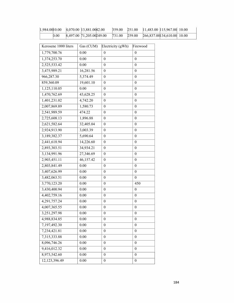
184

1,984.0010.00 4,070.00 13,881.0042.00 359.00 251.00 11,483.00 115,967.00 10.00

0.00 8,497.00 71,205.00249.00 731.00 259.00 266,837.00134,610.00 10.00

Kerosene 1000 liters Gas (CUM) Electricity (gWh) Firewood

1,779,700.76 0.00 0 0

1,374,253.70 0.00 0 0

2,525,533.42 0.00 0 0

3,475,989.21 16,281.56 0 0

966,287.30 5,374.49 0 0

859,360.09 19,601.10 0 0

1,125,110.05 0.00 0 0

1,470,762.69 43,628.25 0 0

1,401,231.02 4,742.20 0 0

2,007,869.89 1,580.73 0 0

2,541,989.59 474.22 0 0

2,725,608.13 1,896.88 0 0

2,621,582.64 32,405.04 0 0

2,924,913.90 3,003.39 0 0

3,189,382.37 5,690.64 0 0

2,441,618.94 14,226.60 0 0

2,893,303.51 34,934.21 0 0

3,134,991.96 27,346.69 0 0

2,903,451.11 46,157.42 0 0

2,803,841.49 0.00 0 0

3,407,626.99 0.00 0 0

3,482,063.51 0.00 0 0

3,770,123.20 0.00 0 450

3,430,400.94 0.00 0 0

4,402,759.16 0.00 0 0

4,291,757.24 0.00 0 0

4,007,365.55 0.00 0 0

3,251,297.98 0.00 0 0

4,988,834.85 0.00 0 0

7,197,492.30 0.00 0 0

7,234,421.81 0.00 0 0

7,315,333.88 0.00 0 0

8,096,746.26 0.00 0 0

9,416,012.32 0.00 0 0

8,973,542.60 0.00 0 0

12,123,396.49 0.00 0 0

185

A6.4 Export of selected traded goods in tons (or indicated otherwise) Wheat Rice Pulses Milk Butter Vegetable

Oil Apple Banana Mutton Beef

107,000.00 230,000.00 249.00 0.00 3.00 4,600.00 17.00 603.00 0.00 18.00

11,000.00 182,193.00 120.00 0.00 0.00 4,600.00 15.00 687.00 0.00 267.00

19.00 197,980.00 18.00 0.00 0.00 0.00 11.00 1,497.00 0.00 331.00

2.00 788,876.00 31.00 0.00 2.00 1.00 8.00 554.00 6.00 156.00

0.00 597,240.00 0.00 0.00 0.00 0.00 0.00 2,510.00 0.00 0.00

0.00 477,650.00 0.00 0.00 0.00 0.00 0.00 3,685.00 0.00 0.00

0.00 794,548.00 0.00 0.00 8.00 0.00 0.00 1,513.00 0.00 2.00

150.00 960,164.00 0.00 0.00 0.00 0.00 0.00 2,000.00 0.00 0.00

0.00 776,600.00 4,000.00 0.00 0.00 0.00 46.00 8,545.00 0.00 0.00

0.00 1,015,010.00300.00 0.00 0.00 0.00 2.00 17,627.00 0.00 0.00

0.00 1,086,640.00490.00 32.00 0.00 0.00 0.00 12,394.00 0.00 0.00

0.00 1,243,670.00425.00 288.00 0.00 0.00 18.00 9,461.00 0.00 0.00

5.00 951,028.00 480.00 0.00 0.00 1.00 0.00 10,834.00 0.00 0.00

99,081.00 904,801.00 847.00 0.00 0.00 3.00 4.00 4,601.00 0.00 8.00

218,642.00 1,265,000.00130.00 0.00 0.00 1.00 0.00 3,213.00 0.00 0.00

47,707.00 718,686.00 806.00 0.00 0.00 1.00 1.00 4,599.00 0.00 0.00

0.00 1,316,020.003,320.00 0.00 0.00 0.00 2.00 5,214.00 0.00 0.00

0.00 1,270,400.003,777.00 0.00 0.00 0.00 0.00 8,631.00 0.00 0.00

2,215.00 2,110,200.003,238.00 0.00 0.00 553.00 0.00 5,955.00 0.00 7.00

0.00 854,320.00 3,746.00 0.00 0.00 0.00 0.00 420.00 0.00 0.00

0.00 743,889.00 10,102.000.00 0.00 1.00 3.00 430.00 15.00 253.00

0.00 1,204,580.003,970.00 0.00 0.00 3.00 1.00 808.00 4.00 216.00

0.00 1,511,840.00466.00 1,060.00 0.00 0.00 5.00 3,609.00 56.00 125.00

0.00 1,032,130.001,509.00 0.00 0.00 0.00 46.00 3,262.00 39.00 76.00

5,039.00 984,325.00 794.00 0.00 0.00 49.00 11.00 1,054.00 15.00 85.00

0.00 1,852,270.00307.00 272.00 0.00 0.00 91.00 2,412.00 10.00 164.00

2,473.00 1,600,520.00722.00 0.00 0.00 0.00 127.00 1,117.00 21.00 257.00

0.00 1,767,210.000.00 0.00 0.00 0.00 536.00 2,500.00 8.00 204.00

4,000.00 1,971,600.00224.00 14.00 0.00 0.00 5,178.003,214.00 119.00 106.00

4,000.00 1,791,190.00402.00 14.00 0.00 0.00 5,134.0039.00 720.00 283.00

23,148.00 2,016,270.00809.00 143.00 0.00 0.00 2,108.00605.00 2,713.00 597.00

353,238.00 2,423,860.004,355.00 312.00 28.00 36.00 888.00 3,801.00 968.00 347.00

642,595.00 1,684,330.004,009.00 1,011.00 40.00 1.00 818.00 3,689.00 517.00 813.00

1,138,281.00 1,819,980.0026,502.003,031.00 35.00 1.00 250.00 7,234.00 2,235.00 1,518.00

42,863.00 1,822,740.0050,929.009,114.00 20.00 0.00 97.00 6,052.00 4,097.00 1,265.00

27,252.00 2,891,390.0033,567.0011,749.00 6.00 3.00 100.00 853.00 3,650.00 2,054.00

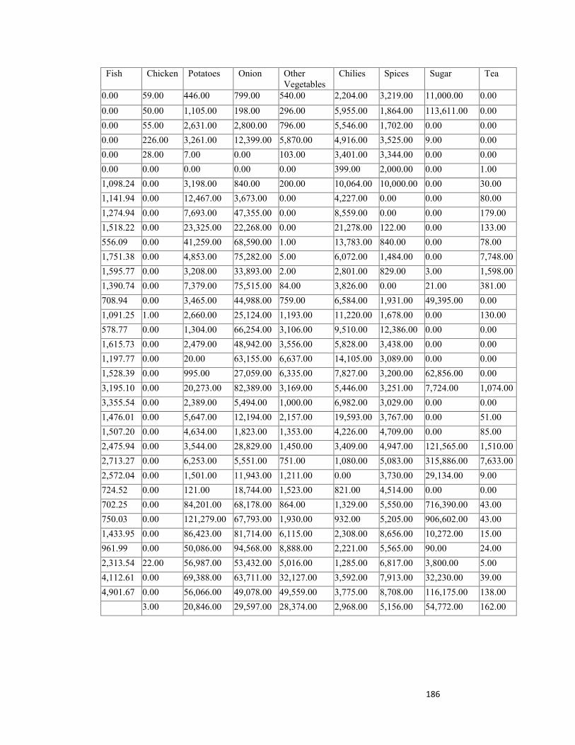
186

Fish Chicken Potatoes Onion Other Vegetables

Chilies Spices Sugar Tea

0.00 59.00 446.00 799.00 540.00 2,204.00 3,219.00 11,000.00 0.00

0.00 50.00 1,105.00 198.00 296.00 5,955.00 1,864.00 113,611.00 0.00

0.00 55.00 2,631.00 2,800.00 796.00 5,546.00 1,702.00 0.00 0.00

0.00 226.00 3,261.00 12,399.00 5,870.00 4,916.00 3,525.00 9.00 0.00

0.00 28.00 7.00 0.00 103.00 3,401.00 3,344.00 0.00 0.00

0.00 0.00 0.00 0.00 0.00 399.00 2,000.00 0.00 1.00

1,098.24 0.00 3,198.00 840.00 200.00 10,064.00 10,000.00 0.00 30.00

1,141.94 0.00 12,467.00 3,673.00 0.00 4,227.00 0.00 0.00 80.00

1,274.94 0.00 7,693.00 47,355.00 0.00 8,559.00 0.00 0.00 179.00

1,518.22 0.00 23,325.00 22,268.00 0.00 21,278.00 122.00 0.00 133.00

556.09 0.00 41,259.00 68,590.00 1.00 13,783.00 840.00 0.00 78.00

1,751.38 0.00 4,853.00 75,282.00 5.00 6,072.00 1,484.00 0.00 7,748.00

1,595.77 0.00 3,208.00 33,893.00 2.00 2,801.00 829.00 3.00 1,598.00

1,390.74 0.00 7,379.00 75,515.00 84.00 3,826.00 0.00 21.00 381.00

708.94 0.00 3,465.00 44,988.00 759.00 6,584.00 1,931.00 49,395.00 0.00

1,091.25 1.00 2,660.00 25,124.00 1,193.00 11,220.00 1,678.00 0.00 130.00

578.77 0.00 1,304.00 66,254.00 3,106.00 9,510.00 12,386.00 0.00 0.00

1,615.73 0.00 2,479.00 48,942.00 3,556.00 5,828.00 3,438.00 0.00 0.00

1,197.77 0.00 20.00 63,155.00 6,637.00 14,105.00 3,089.00 0.00 0.00

1,528.39 0.00 995.00 27,059.00 6,335.00 7,827.00 3,200.00 62,856.00 0.00

3,195.10 0.00 20,273.00 82,389.00 3,169.00 5,446.00 3,251.00 7,724.00 1,074.00

3,355.54 0.00 2,389.00 5,494.00 1,000.00 6,982.00 3,029.00 0.00 0.00

1,476.01 0.00 5,647.00 12,194.00 2,157.00 19,593.00 3,767.00 0.00 51.00

1,507.20 0.00 4,634.00 1,823.00 1,353.00 4,226.00 4,709.00 0.00 85.00

2,475.94 0.00 3,544.00 28,829.00 1,450.00 3,409.00 4,947.00 121,565.00 1,510.00

2,713.27 0.00 6,253.00 5,551.00 751.00 1,080.00 5,083.00 315,886.00 7,633.00

2,572.04 0.00 1,501.00 11,943.00 1,211.00 0.00 3,730.00 29,134.00 9.00

724.52 0.00 121.00 18,744.00 1,523.00 821.00 4,514.00 0.00 0.00

702.25 0.00 84,201.00 68,178.00 864.00 1,329.00 5,550.00 716,390.00 43.00

750.03 0.00 121,279.00 67,793.00 1,930.00 932.00 5,205.00 906,602.00 43.00

1,433.95 0.00 86,423.00 81,714.00 6,115.00 2,308.00 8,656.00 10,272.00 15.00

961.99 0.00 50,086.00 94,568.00 8,888.00 2,221.00 5,565.00 90.00 24.00

2,313.54 22.00 56,987.00 53,432.00 5,016.00 1,285.00 6,817.00 3,800.00 5.00

4,112.61 0.00 69,388.00 63,711.00 32,127.00 3,592.00 7,913.00 32,230.00 39.00

4,901.67 0.00 56,066.00 49,078.00 49,559.00 3,775.00 8,708.00 116,175.00 138.00

3.00 20,846.00 29,597.00 28,374.00 2,968.00 5,156.00 54,772.00 162.00

187

Cigarettes Kerosene (1000 Liters) Gas CUM87 Electricity gWh Firewood

6,000.00 68,259.89 0.00 0 0

574.00 35,214.09 0.00 0.00 0.00

1,162.00 110,117.33 0.00 0.00 0.00

678.00 232,736.26 0.01 0.00 0.00

594.00 39,820.93 0.03 0.00 0.00

3,754.00 29,054.84 0.02 0.00 0.00

5,709.00 71,043.92 0.03 0.00 0.00

4,390.00 71,132.48 0.05 0.00 0.00

3,607.00 73,581.67 0.05 0.00 0.00

1,650.00 176,648.86 0.07 0.00 0.00

2,562.00 110,689.39 0.10 0.00 0.00

991.00 0.00 0.06 0.00 0.00

909.00 16.47 0.00 0.00 0.00

908.00 66.45 0.01 0.00 0.00

690.00 0.00 0.00 0.00 0.00

584.00 0.00 0.00 0.00 0.00

582.00 0.00 0.00 0.00 0.00

518.00 0.00 0.00 0.00 0.00

411.00 123,020.28 0.00 0.00 0.00

286.00 221,364.83 0.00 0.00 0.00

1,464.00 336,287.52 0.00 0.00 0.00

1,998.00 352,357.36 0.00 0.00 0.00

2,469.00 444,478.96 0.00 0.00 0.00

1,171.00 316,748.88 0.00 0.00 0.00

981.00 377,164.34 0.00 0.00 0.00

1,066.00 382,854.12 0.00 0.00 0.00

1,329.00 1,056,145.62 0.00 0.00 0.00

1,226.00 163,013.64 0.00 0.00 0.00

1,642.00 445,124.97 0.00 0.00 0.00

978.00 460,856.45 0.00 0.00 0.00

1,109.00 473,518.96 0.00 0.00 0.00

1,202.00 446,276.05 13.59 0.00 0.00

1,408.00 254,042.62 1.52 0.00 0.00

1,384.00 147,453.19 2.08 0.00 0.00

1,019.00 58,150.75 2.28 0.00 0.00

87 Trade statistics of Kerosene and Gas in (1000 liters and CUM) have been calculated from International prices of crude oil per liter and Average international (1985-2009) price of natural gas per cubic meter and the value of imports and exports in US $.

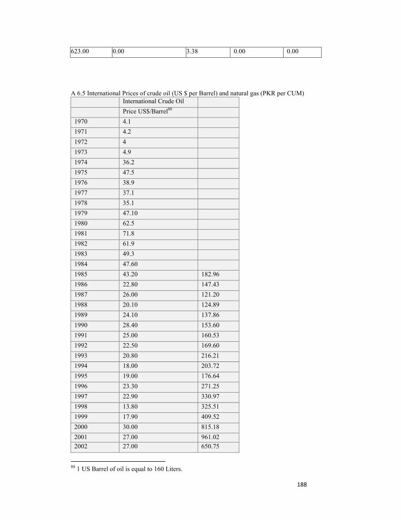
188

623.00 0.00 3.38 0.00 0.00

A 6.5 International Prices of crude oil (US $ per Barrel) and natural gas (PKR per CUM)

International Crude Oil

Price US$/Barrel88

1970 4.1

1971 4.2

1972 4

1973 4.9

1974 36.2

1975 47.5

1976 38.9

1977 37.1

1978 35.1

1979 47.10

1980 62.5

1981 71.8

1982 61.9

1983 49.3

1984 47.60

1985 43.20 182.96

1986 22.80 147.43

1987 26.00 121.20

1988 20.10 124.89

1989 24.10 137.86

1990 28.40 153.60

1991 25.00 160.53

1992 22.50 169.60

1993 20.80 216.21

1994 18.00 203.72

1995 19.00 176.64

1996 23.30 271.25

1997 22.90 330.97

1998 13.80 325.51

1999 17.90 409.52

2000 30.00 815.18

2001 27.00 961.02 2002 27.00 650.75

88 1 US Barrel of oil is equal to 160 Liters.

189

2003 30.00 1051.07

2004 38.30 1217.50

2005 50.10 1715.62

Average 632.62

CV

1. General

Name: Shaikh, Naveed Ahmed, PhD Date of birth: 02.01.1976 Nationality: Pakistan Civil Status: Married Contact: Office: Department of Economics, Shah Abdul Latif University, Khairpur, Pakistan Ph. 0092-243-9280280 Home: 37/192 Saddar Mohalla Shikarpur Sindh Cell: 0092-336-2401093 Email: naveediqbal15@hotmail.com

2. Professional Experience (11 years)

September 2000 to December 2005 Lecturer (Department of EcoShah Abdul Latif University, Khairpur, Pakistan)

December 2005 to date... Assistant Professor (Departm

Economics, Shah Abdul LatifUniversity, Khairpur, Pakistan

3. Academic Record

Degree/Certificate Year University

• PhD 2011 Institute of dev(International Development Studies) Research and

Development PRuhr UniversityBochum, Germ

Thesis Topic: Trade Liberalization, Poverty and Welfare in Pakistan

Supervisor: Prof. Dr. Wilhelm Löwenstein

• M.Phil (Economics) 2003 Department of EcShah Abdul Latif University, KhairPakistan

190

nomics,

ent of )

elopment

olicy,

any

onomics,

pur,

191

Thesis Topic: Information Technology as a catalyst agent for the process of Globalization (A case study of Pakistan)

Supervisor: Prof. Dr. Iqbal Ahmed Panhwar

• MSc Economics 1998-1999 School of Economics, International Islamic University, Islamabad, Pakistan

Cumulative Grade Percentage Average (CGPA): 3.4/4.00 equal to 75.9%

• BSc (Hons) Economics 1994-1998 School of Economics, International Islamic University, Islamabad, Pakistan

Cumulative Grade Percentage Average (CGPA): 2.89/4.00 equal to 70.55%.

• Intermediate (Pre-Eng.) (69%) 1993 C & S Government Degree College Shikarpur

(Board of Intermediate and Secondary Education Larkana)

• Matriculation (84%) 1991 Government High School No.1 Shikarpur

(Board of Intermediate and Secondary Education Larkana)

Remark: English was the major language of instruction throughout the academic career.

4. Conferences, Internships, Trainings, Workshops and Projects

Conferences

• Abstract accepted titled “Selective Trade Protectionism and Trade Liberalization: Impact on Household Welfare in Pakistan (A Marshallian Approach)” for 27th PSDE-PIDE annual conference at Pakistan Society of Development Economists, arranged by Pakistan Institute of Development Economics, Islamabad 16-17 December 2011.

192

• Abstract accepted titled “Trade Liberalization and Wage Inequality: Conflict of Statistical Evidence in the Reviewed Literature” for SZABIST’s International Conference on Management, Social Sciences, Economics and Computing in collaboration with the Faculty of Administrative and Management Sciences, University of Karachi.14-15 December 2011.

Internships

• Three month internship at State Bank of Pakistan (Central Bank) to get the know how about the working of its various sections (2 July 1998-26 August 1998)

Trainings

• 3-month short Course on International Trade, WTO and related Issues at Pakistan Institute of Development Economics, Islamabad, Pakistan ( June - August 2003)

• One year Diploma in Information Technology at Petroman Training Institute Sukkur, Pakistan ( July 2000-June 2001)

Workshops

• Three day Workshop on “Intercultural Communication and Team Building” organized by Institute of Development Research and Development Policy, RUB (15-17 September 2006 at Olpe, Germany )

• “Narration/Mediation: The Constitution of the ‘Self’ in Interdisciplinary Perspective” Section Day Humanities and Social Sciences (November 7, 2008) arranged by Ruhr Research School, Ruhr University Bochum, Germany

• Three day writing Workshop on “Becoming a Better Academic Writer” (14-16 May 2009) at Ruhr Research School, Ruhr University Bochum, Germany.

• Three day Workshop on “Introduction into Structural Equation Modeling using Mplus at Institute of Development Research and Development Policy, Ruhr University Bochum, Germany (17-19 February 2010)

• 3-day Reintegration Seminar arranged by ARBEITSKREIS AFRIKANISCH-ASIATISCHER AKADEMIKERINNEN UND AKADEMIKER Göttingen, Germany (23-25 October 2009)

• 3-Day workshop on Project Proposal writing at Institute for Development Research and Development Policy, Ruhr University

193

Bochum in collaboration with GOPA Consultants. (10-12 March 2010) (Certificate awaited…)

• 2 day workshop on “Social Audit of Governance and Public Service Delivery 2011-2012” by UNDP at Holiday (Islamabad) Hotel, 10-11 January, 2012

Projects

• A Household Survey completed successfully as Research and Logistic Coordinator under the project of Social Audit and Government Services Delivery 2011-2012 under Partnership between UNDP and Shah Abdul Latif University Khairpur funded by UNDP (Amount PKR796500) in January-February 2012. Conducted two-day class and field training of 9 team members and 8 days field survey in four different districts of Khairpur, Sukkur, Shikarpur and Jacobabad. (Amount Rs. 0.8 Million)

• Proposal accepted for Gender Equity Project funded by USAID in partnership with Asia Foundation (Amount Rs. 3 Million)

5. Weakly Business and Finance Review articles: 1. US dollar in the line of fire

Link to access: http://jang.com.pk/thenews/jan2010-weekly/busrev-18-01-2010/p6.htm

2. INTERNATIONAL TRADE : Lessons from experience Link to access: http://jang.com.pk/thenews/feb2010-weekly/busrev-01-02-2010/p5.htm

3. Challenges the new economic advisor is going to face Link to access: http://jang.com.pk/thenews/mar2010-weekly/busrev-29-03-2010/p6.htm

4. Economic Slowdown and rising poverty Link to access: http://jang.com.pk/thenews/may2010-weekly/busrev-10-05-2010/p13.htm

5. Global Outlook: Greek Financial Crisis: Another disaster unleashed Link to access: http://jang.com.pk/thenews/may2010-weekly/busrev-17-05-2010/p4.htm

6. Shift in Global Economic Power Link to access: http://jang.com.pk/thenews/may2010-weekly/busrev-31-05-2010/p4.htm

7. An assessment of Revenues and Expenditures Link to access: http://jang.com.pk/thenews/jun2010-weekly/busrev-14-06-2010/p9.htm

8. Pak-Iran Gas Pipe Line Link to access: http://jang.com.pk/thenews/jul2010-weekly/busrev-12-07-2010/p4.htm

9. Pak-US Strategic Dialogue

194

Link to access: http://jang.com.pk/thenews/jul2010-weekly/busrev-26-07-2010/index.html#1

6. Research Publications

1. Shaikh, N. A. & Memon, A.L, (2000); “Credit Creation in general & Banking Practice in Pakistan” The Commerce & Economic Review, Vol. XI 2000-01, Shah Abdul Latif University Khairpur, Pakistan

2. Shaikh, N. A. & Memon, A.L, (2002); “Impact of war against terrorism on Pakistan Economy” The Commerce & Economic Review, Vol. XII 2002-03, Shah Abdul Latif University Khairpur, Pakistan

3. Shaikh, N. A. & Sahito, I. H. Dr, (2002) “Role of Microcredit in Economic Revival and Poverty Alleviation” The Commerce & Economic Review, Vol. XII 2002-03, Shah Abdul Latif University Khairpur, Pakistan

4. Jamali, M. B. Dr.; H. Jawad, Shaikh, N. A. Dr; Shaikh, F. M, Afridi, T. (2011) “Internationalization of SMES and Organizational factors in developing countries: A case study of ice industry in Pakistan” Australian Journal of Business and Management Research Vol. 1, No. 7 [129-138] | October

5. Shaikh, N. A. Dr.; Mangi, R. A.; Soomro, H. J.; (2011) “Trade Liberalization and Wage Inequality: Conflict of Statistical Evidence in the Reviewed Literature: Experience of Latin American and East Asian Countries corresponding to the theoretical findings of Heckscher-Ohlin Trade Theorem” Interdisciplinary Journal of Contemporary Research in Business, Vol. 3, No.8, Dec. [965-971]

6. Bhatti, N., Maitlo, G. M., Shaikh, N. A. Dr., Hashmi, M. A., Shaikh, F. M., (2012) “The Impact of Autocratic and Democratic Leadership Style on Job Satisfaction” International Business Review, Vol. 5, No. 2; Feb.[192-201] www.ccsenet.org/ibr .

7. Bhatti, N., Phulpoto, L.A, Shaikh, N.A. Dr, Afridi, T., Shaikh, F.M (2012) “Economic and Social Factors of Poverty: A case study of Sindh” Journal of Management and Sustainability, Vol. 2 No.1, March.[227-234]

8. Shaikh, S.; Shaikh, N.A. Dr. (2012) “Impact of FDI, Capital Formation and International Trade on Economic Growth of Pakistan: An Empirical Analysis” Interdisciplinary Journal of Contemporary Research in Business, Vol. 3, No. 11, March.

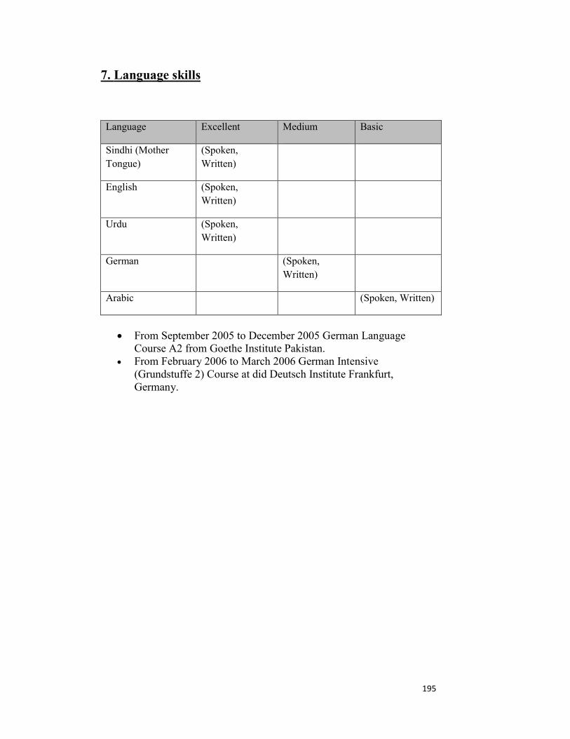
195

7. Language skills

Language Excellent Medium Basic

Sindhi (Mother Tongue)

(Spoken, Written)

English (Spoken, Written)

Urdu (Spoken, Written)

German (Spoken, Written)

Arabic (Spoken, Written)

• From September 2005 to December 2005 German Language

Course A2 from Goethe Institute Pakistan. • From February 2006 to March 2006 German Intensive

(Grundstuffe 2) Course at did Deutsch Institute Frankfurt, Germany.