Trade Barriers and Trade Flows with Product Heterogeneity:

An Application to US Motion Picture Exports

Gordon Hanson, UC San Diego and NBER

Chong Xiang, Purdue University and NBER

October 2010

Abstract

We extend Melitz (2003) to allow for both global and bilateral fixed export costs. If global (bilateral) export costs dominate, the average sales ratio (import sales per product variety/domestic sales per variety), decreases (increases) in variable (fixed) trade barriers, due to adjustment along the intensive (extensive) margin of trade. Using novel data on bilateral US movie exports we find that (i) variation in box-office revenues per movie is much larger than in the number of movies exported, and (ii) the average sales ratio decreases in geographic and linguistic distance. These findings suggest that global fixed export costs dominate. _____________ Hanson: gohanson@ucsd.edu; Xiang: cxiang@purdue.edu. We thank David Hummels, Marc Melitz, Phillip McCalman, Nina Pavcnik, Stephen Redding, and seminar participants at UCSD, the NBER, the Princeton University IES Workshop and the 2008 EIIT Meetings for helpful comments; Adina Ardelean, Sirsha Chatterjee, Anca Cristea, Michael Ewens, and Jeffrey Lin for excellent research assistance; and the National Science Foundation for financial support.

1

I Introduction

Fixed trade costs have become a common feature of international trade models. To explain why most manufacturing plants do not export any output and why those that do are relatively large and productive (Bernard and Jensen, 1999 and 2004), Melitz (2003), in widely cited work, develops a model with firm heterogeneity and fixed export costs. Because of fixed trade charges, only more productive plants find it profitable to sell goods abroad.1 Fixed trade costs imply that adjustment in trade volumes may occur along both the intensive margin (value of trade per product) and extensive margin (number of products traded). In the standard monopolistic competition model, consumer love of variety leads all products to be exported, meaning trade varies at the intensive margin only (Helpman and Krugman, 1985). A fall in transport costs causes exports of all products to increase, consistent with the robust negative coefficient on distance in the gravity model of trade (Anderson and van Wincoop, 2004). With fixed export costs and firm heterogeneity, a fall in transport costs may cause trade volumes to increase both through existing exporters exporting more and new firms beginning to export. Bernard, Jensen, Redding, and Schott (2007) find that most variation in US merchandise exports is at the extensive margin, with smaller countries importing fewer US products. Despite abundant indirect evidence that fixed trade costs exist, we know little about their nature. While we can measure variable trade barriers in the form of tariffs or transport fees, no similar data exist for expenses that are fixed. If fixed export costs are bilateral, such that firms incur a charge to enter each new foreign market, small countries will be disadvantaged in global trade. However, if fixed export costs are largely global in nature, such that once firms establish an international distribution network they face only variable charges in adding new markets, small countries are not at a disadvantage and it is only less productive firms that fail to participate in trade. In this paper, we develop a version of the Melitz (2003) model with both global and bilateral fixed export costs. For countries where global fixed export costs are large relative to bilateral costs, import sales per product variety (relative to domestic sales per variety) are decreasing in variable trade barriers, as adjustment occurs along the intensive margin of trade. For countries where bilateral fixed export costs are relatively large, imports per product variety are increasing in fixed trade barriers, due to adjustment occurring along the extensive margin. When global fixed export costs are sufficiently large, they dominate for all countries, such that bilateral fixed export costs have no significant effects on export decisions. In contrast, when global export costs are sufficiently small, bilateral fixed export costs dominate for all countries. Whether or not global fixed export costs dominate, and for which countries they dominate, depend on the magnitudes of fixed export charges and are therefore empirical questions. In US manufacturing, most adjustment to trade barriers is at the extensive margin, suggesting that bilateral fixed export costs dominate. This conclusion, however, is impressionistic, as the literature lacks formal analysis of the relative importance of global versus bilateral fixed export costs or whether results for manufacturing generalize to other sectors. We apply our framework to data on exports of US motion pictures. An advantage

1 When applied to aggregate data, this framework yields a gravity specification that can account for why many country pairs do not trade (Helpman, Melitz, Rubinstein, 2007; Baldwin and Harrigan, 2007).

2

of our approach is that we need not take a stand on which trade barriers represent fixed impediments and which variable ones. The empirical literature offers little guidance on the issue. Standard gravity variables – distance, language, colonial history – are likely correlated with variable and fixed barriers. We exploit the divergent predictions of the two regimes for whether imports per variety have positive or negative correlation with trade barriers, making our approach applicable in a wide variety of settings. The characteristics of the film industry are consistent with the assumptions of the Melitz framework. Fixed costs are important in movie production and studios differentiate their film product (De Vany, 2004). There is heterogeneity in movie performance, with box-office revenues for US films exhibiting heavy right tails (De Vany and Walls, 1997, 2004). Not all US movies are exported, with the typical country importing half of the movies the US produces in a given year. Given the absence of published data on bilateral trade in motion pictures,2 we construct a new data set using information from ScreenDigest.com, an entertainment industry consultancy, which includes box-office revenues for domestic and US movies in 46 countries over 1995-2006. We also make use of data on trade barriers in motion pictures from other sources. A broader motivation for studying motion pictures is that the vast majority of empirical work on trade is for manufacturing, with relatively little work on services. Exports of services such as motion pictures are distinct from exports of manufactures in that variable production costs (e.g., exhibiting movies to consumers) are incurred in the country of consumption, rather than the country of production, and the physical cost of transporting goods abroad (e.g., shipping master film prints) is close to nil. For motion pictures and other cultural goods, cross-country differences in language, social mores, or religion may be the significant barriers to trade (Rauch and Trindade, 2009). Movies are representative of other information services, including music, publishing, software, television, and video games, which are responsible for a growing share of US trade. These “copyright” industries tend to have large fixed production costs (associated with creating an initial film print, music recording, or software program) and small marginal production costs (associated with producing additional copies). In 2007, copyright industries accounted for 7% of US GDP; US movies, TV, and videos had foreign sales plus exports of $20 billion, just below that for US pharmaceuticals. Our main finding is that a model in which global fixed export costs dominate for all countries in the sample best explains US exports of motion pictures. Imports per product variety are decreasing in geographic distance, linguistic distance, and other measures of trade barriers, in a manner consistent with adjustment to these barriers occurring along the intensive rather than the extensive margin. There is relatively little variation in the number of US movies that countries import but wide variation in the box-office revenues per movie, with countries more distant from the US spending less on the US movies that they see. Argentina, for instance, imports roughly the same number of US movies each year as Germany, though the box office revenues per US film there are far lower. These results hold across groups of importers separated by size or distance from the United States, suggesting that in our sample, bilateral fixed export costs dominate for few, if any, countries. Whereas the gravity-equation literature consistently

2 For exports of US movies, McCalman (2005) has foreign release dates but not foreign revenues. The US government does not publish trade flows for movies. UN Comtrade lists motion pictures as a commodity; its trade data understate foreign box-office revenue by several orders of magnitude (see note 21).

3

finds a negative correlation between log sales and geographic and linguistic distance, our specification is based on a double difference in the form of log sales per product among imports minus log sales per product among domestic goods. Our finding is, therefore, not a corollary of results in the gravity literature. We are unaware of previous literature that uses such a specification in testing trade models. In section II, we present the model and estimation strategy. In section III, we discuss data and preliminary data analysis. In section IV, we present empirical results and in section V, we conclude. II Theory

In this section, we extend the Melitz model and allow fixed export costs to have both bilateral and global components. The bilateral components are incurred each time a producer enters a new export market; the global components are incurred once, when a producer starts exporting. The model predicts that the correlation between trade costs and revenues per movie depends on whether the global components of fixed export costs dominate the bilateral ones or vice-versa.

IIA Model Setup

There are many sectors, over which consumers have Cobb-Douglas preferences, and T + 1 countries, where u indexes the exporter and k = 1…T indexes the importers. We focus on the movie industry and leave other sectors in the background.

Movies are subject to cultural discount (Waterman, 2005). For a consumer in country k, a movie from country u (the US) reduces utility by δuk as compared with a domestic movie, where 0 < uk < 1. Similar to a pure iceberg trade cost, δuk is the portion of a movie’s value that is not “lost in translation” in moving from one country to another. We expect δuk to be higher the more similar are two countries’ culture and language.

Movies are also subject to fixed and variable trade costs. Variable ad valorem trade fees, defined as tuk > 1, include tariffs and surcharges on foreign movie revenues (Marvasti and Canterbery, 2005), transaction costs in negotiating contracts between US movie distributors and foreign movie exhibitors (Gil and LaFontaine, 2009),3 advertising expenses (which depend on the length of time a movie spends in theatres), and film printing expenses (which depend on the number of times a movie is shown and the number of theatres in which it appears). Fixed export costs are associated with allocating the right to distribute a movie in different countries, creating an international marketing campaign, editing movies for foreign audiences, and adding subtitles or dubbing movie dialogue. Fixed costs may be market specific (if each country requires its own marketing campaign) or global in nature (if one marketing campaign serves multiple countries). Fixed and variable trade charges may have common underlying determinants, with distance, language, and the costs of enforcing contracts possibly affecting both.

3 Gil and LaFontaine (2007) find that in the Spanish movie industry distributors sign an initial contract for sharing revenues with movie exhibitors, which may be renegotiated multiple times, as a movie reveals itself to be more or less popular than expected. Contracting costs are thus a function of the level of revenues and not simply the discrete outcome of whether or not a movie is shown.

4

The subutility for movies for the representative consumer in country k is CES,4

uk = 1 1

1{ [ ] }j u k jj kj j uk ujc c

, (1)

where σ > 1 is the substitution elasticity. A demand shifter, θj, captures heterogeneity in movies. A movie with a high θj is popular (E.T., Titanic); one with a low θj is unpopular (Ishtar, Gigli). In line with previous literature on firm heterogeneity, we assume the popularity of a movie does not depend on the country in which it is shown and that θj is drawn from a common distribution, G(θ). Consistent with this assumption, top grossing movies tend to be the same across countries. For individual US-made movies in 2000, the correlation between domestic and foreign box-office revenues is 0.81 (Scott, 2004). Heterogeneity in demand is isomorphic to heterogeneity in marginal costs (Melitz, 2003). We introduce heterogeneity on the demand side as it compresses variation in admission prices for movies within a country, consistent with the data (De Vany, 2004). From (1), box-office revenues (total sales) of a country-u movie in country k are

1 1 1 11

, kukj j uk uk ukj k k

k

Ys t p A A

P

, (2)

where j indexes the movie, Yk and Pk are income and the CES price index in country k, α is the expenditure share for the movie industry, and pukj is the price of movie j (not including the policy trade barrier). In equation (2), both the cultural discount and the policy trade barrier appear as variable trade costs and have similar effects on the sale of movie j. Box-office sales of domestically produced movie h in country k equal,

skkh = 1 1h kkh kp A . (3)

We assume movie production occurs in five steps. (i) A producer in country u hires fE units of country-u labor to produce a master film print, which is a sunk labor input. (ii) The producer draws a θ from the distribution G(θ). (iii) The producer incurs a fixed production cost of b units of country-u labor. (iv) The producer uses a variable labor input to exhibit the movie to an audience, with input costs incurred in the country where the audience is located. For each unit of the movie shown in country k, the producer hires one unit of country-k labor. And (v) the producer collects profits.

In our model, each firm produces a single variety, as in Melitz (2003). However, our setting also has a multi-product-firm interpretation, consistent with Bernard, Redding and Schott (2006). Most movies are distributed by large studios, which may be involved in production as well.5 Even though there are a large number of studios worldwide, a half dozen distribute most high-grossing films (Columbia/MGM, Paramount, Disney, Warner Brothers, 20th Century Fox, and Universal Pictures). One can think of a studio as a multi-product firm. Within a year, a studio will release many movies, where each is a product

4 We specify consumer preferences using the discrete choice framework in Hanson and Xiang (2008) and obtain similar results to those reported here. 5 Making a movie involves development (securing rights, screen writing, casting, financing), production (filming, special effects, music, editing), distribution (marketing, negotiating with theatres), and exhibition. While studios are usually involved in distribution, they have varying roles in earlier stages, sometimes handling a movie from start to finish (Paramount and Mission: Impossible II) and sometimes buying distribution rights to an already finished movie (20th Century Fox and Little Miss Sunshine). US antitrust rulings prevent movie studios from owning theatres, keeping studios out of exhibition.

5

variety. The short lived nature of movies allows studios to differentiate movies in time,6 avoiding the simultaneous release of two or more films. In this setting, for each product variety we can still apply assumptions (i)-(v) and proceed with the analysis.7

Following Melitz (2003), we assume the movie industry is monopolistically competitive.8 By assumption (iii), for a movie created in country u its showings are provided using labor in the country where consumers watch the movie. Since price is a constant markup over marginal cost, the price of a movie shown in country k is the same for all movies, regardless of where they are produced:

pkkj = pukj = 1 kw

for all u, k, j, (4)

where wk is the wage in country k. Because the cultural discount is a source of home bias in demand, it does not affect prices (Anderson and van Wincoop, 2004). Similarly, θj affects the quantity demanded but not prices. Equation (4) implies that in any market k, the prices of domestic and foreign movies are the same.

IIB Decision for Exports

In this sub-section we consider the export decisions by the producers of country-u movies. We show how the pattern of exports depends on bilateral and global fixed export costs, and derive the expressions for the number of exported movies and their total sales abroad. We allow the producers to observe their type before making the export decision, consistent with the movie industry where producers release films on the domestic market first, and then, if they are successful, abroad.9 The export decision for a given country-u movie j involves the comparison between its variable profits abroad and fixed export costs. Equations (2) and (4) imply that the variable profits for movie j in country k equal

1ukj j kDQ ,

1( 1)D

, 1 1 1

k uk uk k kQ t w A , (5)

where Ak is defined in equation (2) and D is a constant. Intuitively, the Q-index, Qk, represents access to country-k market from country u. Market access is relatively strong

6 By the end of three weeks, the average movie has earned 66% of its total box-office revenues (De Vany and Walls, 1999). 7 Multi-product firms bring two additional elements into consideration. First, the popularity of a movie may depend on the “ability” of its studio. Following Bernard, Redding and Schott (2006), we assume the distribution of studio abilities is independent of θ and that the ability of a given studio is common for all products. With each studio randomly drawing its ability when it enters the market, studio abilities are given for each individual movie. Second, the entry decisions and numbers of studios in the market may depend on studio-level sunk entry costs and per period studio-level fixed costs, as well as studio-level ability. Since we lack data on the distribution of movies by studio, we leave studios in the background of the analysis. Some portion of our product-level sunk entry cost fE might be indistinguishable from the studio-level fixed cost, but fE also remains in the background. 8 While the number of major movie studios is small, the number of top talents involved in a movie (e.g., actors, directors, screenwriters, technicians, and producers) is large. Competition between the top talents is important for the competition between movies. To secure the star power of these talents, studios bid for their services (Waterman, 2005), driving expected profits toward zero. Alternatively, suppose the movie producers have more market power than in the monopolistic competition setting. This implies a higher markup in equation (4), but otherwise does not affect our results qualitatively. 9 McCalman (2005) shows that movies released simultaneously in the US and a few foreign markets are released in other foreign markets with a lag.

6

for high Q-index countries, which have a relatively large GDP, Yk, and/or relatively low variable trade costs, δuk and tuk.

Fixed export costs for movie j consist of the global component of fG units of country-u labor, and the bilateral components of fuk units of country-k labor.10 This means that the total fixed export cost to show movie j in countries k = 1…K equals wufG +

1

K

k ukkw f

. Consider the bilateral components first. Conditional on showing movie j

abroad, showing it in an additional country, k, requires the additional fixed export cost wkfuk, and brings in the additional variable profit πukj. Therefore, conditional on showing movie j abroad, it is shown in country k if and only if πukj - wkfuk ≥ 0, or

θj ≥

11 1 1

uk uk uk kuk

k

f t w

DA

. (6)

Equation (6) is the export constraint imposed by the bilateral fixed export costs, and the expression for uk does not depend on the global fixed export costs, fG. Rank the uk ’s

for all the T importing countries from low to high and re-label the countries according to the rank order of the uk ’s; i.e., 1u < 2u < … uT . This ranking of the uk ’s is

illustrated in Figure 1. Country 1 is the most accessible destination market for country-u movies (e.g., the U.K.) and country T is the least accessible destination market for country-u movies (e.g., Latvia). To determine which movies are exported and which are not, start from the movies with the lowest θ’s. First, the movies with θj ≤ 1u (i.e., those to the left of 1u in Figure

1) do not satisfy equation (6) for any importer and so they are not exported. Intuitively, the variable profits for these movies from the most accessible destination market, country 1, are insufficient to pay for the fixed export cost specific to that country, w1fu1, let alone the additional global fixed export cost, wufG. Next, the movies with θj ( 1u , 2 ]u do not

satisfy equation (6) for the importers 2…T and so they are not exported to those countries. However, these movies satisfy equation (6) for country 1, and they will be shown in country 1 if they satisfy the additional condition that 1 1 1u j u u Gw f w f . (7)

Equation (7) says that the variable profits from country 1 can cover both the bilateral and global components of fixed export costs. Since fG > 0, the movie with 1u does not satisfy

equation (7). Suppose equation (7) holds for some movie with θ0 ( 1u , 2 ]u . Then

equation (7) also holds for all the movies with θj ≥ θ0, because these movies bring in more variable profits than the one with θ0 but face the same fixed export costs. Therefore, for these movies with θj ≥ θ0 the pattern of exports is the same as in the standard Melitz model, with bilateral fixed export costs only. That is, the movies with θj [θ0, 2u ) are

exported to country 1, those with θj [ 2u , 3)u are exported to countries 1 and 2, etc.

10 We make this assumption to keep our exposition concise. If, instead, both global and bilateral fixed export costs are in units of country-u labor, the only noticeable change to our results is that equation (16) will have the additional term, wk. This suggests augmenting our main estimation equation, (17), with importer characteristics. We experimented with these additional controls in Hanson and Xiang (2008); they were statistically insignificant and had little effect on our results.

7

Now suppose equation (7) does not hold for any θj ( 1u , 2 ]u . Then we can

examine whether some movie in the range ( 2u , 3u ] satisfies the condition 2

1( )ukj k uk u Gk

w f w f

. If it does, then we can pin down the pattern of exports as

discussed above. If it does not, then we examine whether some movie in the range ( 3u ,

4u ] satisfies the condition 3

1( )ukj k uk u Gk

w f w f

, etc.

Summarizing this algorithm, for movie j to be exported,

θj ≥ G = 1

min { ( ) }j

K

ukj k uk u Gkw f w f

,

where K is such that uk < G for all k ≤ K and , 1u K > G . (8)

Equation (8) is the export constraint imposed by the global fixed export costs. It says that the variable profits from the inframarginal importers 1…K, net of the bilateral fixed export costs specific to these countries, remain sufficient to cover the global fixed export cost. A country-u movie is exported if and only if it satisfies both equations (6) and (8). Figure 1a illustrates the pattern of exports. The value of uk lies between uK and , 1u K .

None of the movies with θj < G gets exported since they do not satisfy equation (8). All

the movies with θj ≥ G are exported to at least the inframarginal K countries 1…K since

they also satisfy equation (6) for these countries. In addition, the movies with θj [ G ,

, 1u K ) are exported to the inframarginal importers 1…K, those with θj ( , 1u K , , 2u K ]

are exported to importers 1…K+1, etc. This pattern of exports suggests the following partition of importers. Let G (for Global) denote the set of inframarginal importers k = 1…K, for which uk < G . These

countries have high Q-indices (i.e., large market size and/or low variable trade costs with country u) and are the most accessible destination markets for country-u movies. For these countries, the global fixed export cost dominates the bilateral ones, and the global export constraint of equation (8) is more binding. Let B (for bilateral) denote the set of importers k = K+1, …,T, for which uk > G . These countries have low Q-indices (i.e.,

small market size and/or high variable trade costs) and are the least accessible markets for country u. For them, bilateral fixed export costs dominate global ones, and the bilateral export constraint of equation (6) is more binding. The relative size of the sets G and B depends on the size of the global fixed export costs relative to bilateral fixed export costs.11 As the global fixed export cost, fG, increases, G increases by equation (8) but uk remains unchanged by equation (6). This

implies that the set G expands to encompass more countries, ceteris paribus. We illustrate these changes using Figure 1b. The increase in fG increases G from a value in

the range ( uK , , 1u K ) to a higher value in the range ( uL , , 1u L ), where L > K.12 As the

11 The analytical solution for G is difficult to obtain, since G depends on the levels and distributions of

fuk and Qk. 12 This also shows that the increase in fG has a discrete effect on the composition of the set G, which

changes only if G rises above , 1u K .

8

line corresponding to G shifts to the right, the set G expands to incorporate the

additional countries {K+1,…,L}, and the set B contracts accordingly. In addition, if the increase in fG is sufficiently large, the line G could shift to the right of uT , in which

case the set B is empty and all importers are in the set G. In this case, the global fixed export cost dominates for every importer and the bilateral fixed export costs play no role in the decision for exports. The other polar case is when global fixed export cost is very small so that the set G is empty.13 Then, bilateral fixed export costs dominate for every importer, as if the global fixed export cost did not exist. We now derive (a) the number of country-u movies exported to country k, and (b) total sales of country-u movies in country k,, for the G and B sets of importers. Following the literature on the Melitz model we assume that the distribution function G(·) is Pareto with G(θ) = 1 – aς/θς, where a, ς > 0 and θ [a, ). A large ς means thin tails for G(θ). We assume that ς > σ-1, such that total movie sales are finite. Let Nu denote the number of country-u movies that draw from the distribution G(θ).14 First, by equation (8) and Figure 1, the G set of importers share the common export cut-off of G . Using the value of G we have:

(a) nuk = ( )G

u ujN dG

= ( ) ,u GN a k G,

(b) ( )G

uk u ukj ujS N s dG

= 1

1 1 1 ,( 1)

Gu uk uk uk k k u

DC n t A w C

, k G, (9)

To see the intuition behind (9), consider the total sales of country-u movies in country k, Suk. Equation (9b) is a gravity-like prediction in which Suk responds to country-k characteristics, such as income, and variable trade costs between u and k. This variation consists of an extensive margin – the number of country-u movies exported to k – and an intensive margin – the average sale per country-u movie. In (9a), the extensive margin is exporting-country specific and does not vary with importing-country characteristics. As a result, all variation in Suk occurs along the intensive margin. The fixed export cost does not affect the intensive margin because it does not vary across the G set of importers. Next, for the B set of importers, we can use the values of uk to derive

(a) nuk = ( )uk

u ujN dG

= ( )ukuN a , k B,

(b) ( )uk

uk u ukj ujS N s dG

= 1 1 1 1( )( 1) uku uk uk k k

B aN t A w

= ( 1)uk uk kn f w

, k B, (10)

In contrast to (9), (10) says that variation in Suk across the B set of importers k occurs primarily along the extensive margin, nuk, and that the intensive margin, Suk/nuk, does not

13 Theoretically, this case obtains when equation (7) holds for some movie with θ0 ( 1u , 2 ]u . 14 As in Melitz (2003), Nu is pinned down by the sunk entry cost, fE. In Hanson and Xiang (2008) we derive Nu assuming T+1 identical countries and each country having one sector, as in Melitz (2003). Nu and its counterparts in other countries are jointly determined.

9

depend on variable trade costs, δuk and tuk, or expenditure on movies by k.15 To see the basis for this result, compare importing country l, which has low variable trade costs with exporting country u, to importing country m, which has high variable trade costs with u. Higher variable trade costs in m mean that total sales of country-u movies in m are lower than in l. They also imply a higher cut-off level of θ for country-u movies shown in m, such that m imports a smaller number of movies from u. Given the assumption that the distribution of movie types is Pareto,16 these two effects exactly offset each other, leaving sales per movie unaffected by variable trade costs.17

IIC Decisions for Domestic Production

We now consider domestic movie production in the importers k = 1…T. The decision for domestic production involves the comparison between the variable profits from the domestic market and the fixed production cost parameter, b. To minimize notation, we assume that b is invariant across importers. Since the distribution of θ has support [a, + ), the lowest variable profit a

country-k movie can reap in the domestic market is 1 1k ka A Dw by equations (3) and

(4), where D is a constant defined in equation (5). If this lower bound for variable profit exceeds the fixed production cost, bwk, then the number of country-k movies produced, nkk, equals the number of country-k movies that draw from G(θ), Nk. Intuitively, the fixed production cost is relatively small and so does not affect the decision for domestic production. However, if the lower bound for variable profit is less than bwk, then of the Nk domestic movies that could be made, only those that can at least break even in the domestic market are actually made; i.e., nkk < Nk. The intuition is that the fixed production cost b is relatively large and so it affects which movies are produced domestically. Summarizing

nkk < Nk if b > kb , kb = 1k ka A Dw ; otherwise nkk = Nk. (11)

Equation (11) is the constraint for domestic production imposed by the fixed production cost. In the importers with a large domestic market, Ak, domestic movies collect high variable profits; as a result, kb is large and the constraint for domestic production is less

15 An importing country with a large GDP, Yk, may also have a large number of domestic movies and so a low CES price index, Pk. This tends to reduce the demand for foreign movies and may dampen the effect of Yk. In a stylized model, Helpman, Melitz and Yeaple (2004) show that the competition effect of Pk may completely offset the country-size effect of Yk in general equilibrium such that nuk is the same across all importing countries k. This result is derived under factor-price equalization and identical trade costs for every country pair, assumptions we do not impose. 16 In Hanson and Xiang (2008) we show that our results are robust to alternative assumptions. In particular, we show that under a two-segment Pareto distribution equations (14) and (16), our main estimating equations, need to be augmented by 2nd-order terms of importer characteristics, such as GDP and population. We then estimate the augmented regressions and find that these 2nd-order terms are jointly insignificant. 17 Suppose that there is convex market access cost as in Arkolakis (2007). To derive analytical solutions for Suk we consider the Arkolakis setting with his parameters α, β and γ set to 0. Then the only noticeable changes to our results are (a) the expression for sukj is multiplied by the fraction of consumers that the producer of movie j reaches in country k, (b) equation (10b) becomes Suk = nukfuk(wk – 1)c1, where c1 is a constant, and (c) wk enters into equation (16). These changes do not affect our results qualitatively, as we discuss in note 10.

10

likely to be binding. Rank the importers in descending order in terms of their kb ’s so that

1b > 2b > … Tb . For ease of exposition suppose that Mb > b > 1Mb . Then we can

partition the importers into two sets. Let GD denote the set of importers k = 1…M, for which kb > b. These countries have large domestic markets and so for them the constraint

for domestic production is not binding. Let BD denote the set of importers k = M+1…T, for which kb < b. These countries have small domestic markets and so for them the

constraint for domestic production is binding. Figure 2 illustrates the sets GD and BD. We now derive (a) the number of country-k movies actually made, and (b) the total sales of domestic movies. For the GD set of importers,

(a) nkk = kN .

(b) ( )kk k kkh khaS N s dG

= 1 1

0 0, [ ]( 1) ( 1)

kk k kC n w A C

a

. (12)

For the BD set of importers, a given domestic movie h is made if and only if the variable

profits from the domestic market exceeds the fixed production cost; i.e., 1 1h k kA Bw ≥

bwk. This is equivalent to θh ≥

1

1k

kkk

bw

BA

. Using the value of kk we have

(a) nkk = ( )kk

k khN dG

= ( )kkkN a ,

1

1k

kkk

bw

BA

(b) 1 1( ) ( )( 1)kk

kkkk k kkh kh k k k

B aS N s dG N A w

= ( 1)kk kn bw

. (13)

IID Main Estimating Equations

We now have two ways of partitioning the importers, first using the global and bilateral fixed export costs and then using the fixed production cost. In general, these two approaches produce different partitions. However, country size determines both the ranking of uk and the ranking of kb (e.g., Japan is a large country for U.S. movies and

also a large country for Japanese movies), and so the ranking of uk and the ranking of

kb could be highly correlated. For ease of exposition we assume that18

Assumption 1 G = GD and B = BD. Assumption 1 implies that for the G set of importers where the global fixed export cost dominates, the constraint for domestic production is not binding. Equations (9) and (12) imply that 18 Without Assumption 1, we need to derive the estimating equations for the countries in both G and BD, and for those in both B and GD. We derive these additional equations in Hanson and Xiang (2008), and show that they have little impact on the estimation results, suggesting that the data are consistent with Assumption 1, at least for the countries in our sample.

11

/

ln( ) (1 ) ln( ) ln/

uk uk uku

kk kk uk

S n tC

S n

,

1

( 1)u

u

BC

. (14)

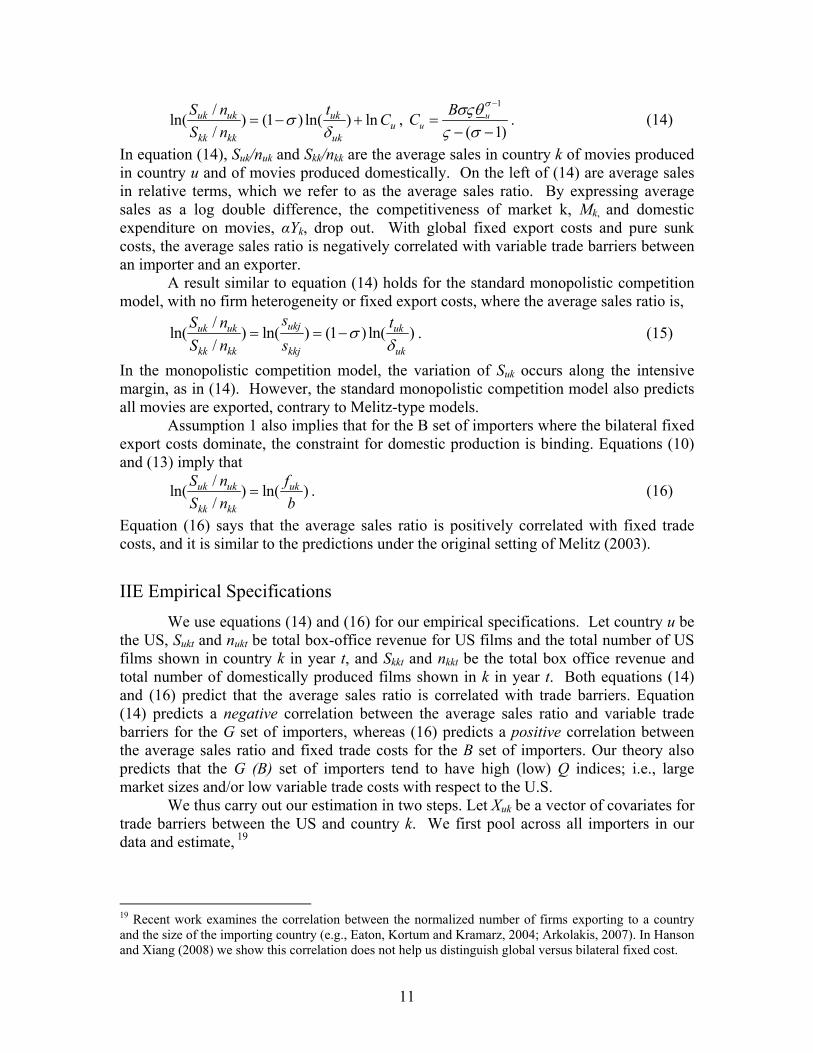
In equation (14), Suk/nuk and Skk/nkk are the average sales in country k of movies produced in country u and of movies produced domestically. On the left of (14) are average sales in relative terms, which we refer to as the average sales ratio. By expressing average sales as a log double difference, the competitiveness of market k, Mk, and domestic expenditure on movies, αYk, drop out. With global fixed export costs and pure sunk costs, the average sales ratio is negatively correlated with variable trade barriers between an importer and an exporter.

A result similar to equation (14) holds for the standard monopolistic competition model, with no firm heterogeneity or fixed export costs, where the average sales ratio is,

/

ln( ) ln( ) (1 ) ln( )/

ukjuk uk uk

kk kk kkj uk

sS n t

S n s

. (15)

In the monopolistic competition model, the variation of Suk occurs along the intensive margin, as in (14). However, the standard monopolistic competition model also predicts all movies are exported, contrary to Melitz-type models. Assumption 1 also implies that for the B set of importers where the bilateral fixed export costs dominate, the constraint for domestic production is binding. Equations (10) and (13) imply that

/ln( ) ln( )

/uk uk uk

kk kk

S n f

S n b . (16)

Equation (16) says that the average sales ratio is positively correlated with fixed trade costs, and it is similar to the predictions under the original setting of Melitz (2003).

IIE Empirical Specifications

We use equations (14) and (16) for our empirical specifications. Let country u be the US, Sukt and nukt be total box-office revenue for US films and the total number of US films shown in country k in year t, and Skkt and nkkt be the total box office revenue and total number of domestically produced films shown in k in year t. Both equations (14) and (16) predict that the average sales ratio is correlated with trade barriers. Equation (14) predicts a negative correlation between the average sales ratio and variable trade barriers for the G set of importers, whereas (16) predicts a positive correlation between the average sales ratio and fixed trade costs for the B set of importers. Our theory also predicts that the G (B) set of importers tend to have high (low) Q indices; i.e., large market sizes and/or low variable trade costs with respect to the U.S.

We thus carry out our estimation in two steps. Let Xuk be a vector of covariates for trade barriers between the US and country k. We first pool across all importers in our data and estimate, 19

19 Recent work examines the correlation between the normalized number of firms exporting to a country and the size of the importing country (e.g., Eaton, Kortum and Kramarz, 2004; Arkolakis, 2007). In Hanson and Xiang (2008) we show this correlation does not help us distinguish global versus bilateral fixed cost.

12

/

ln/

ukt ukt

kkt kkt

S n

S n

αu + αt + βXuk + εukt, (17)

where αt represents year fixed effects and αu is a constant (the U.S. is the only exporting country in our data). The first step reveals whether global or bilateral fixed export costs are the salient feature of our data. If most importers in our data are in the G set, then by equation (14) we have that β ≤ 0; if most of our importers are in the B set, then by equation (16) β ≥ 0. To identify which importers are in the G and B sets, we partition the importers in our data into two sub-samples, those with high apparent Q-indices (i.e., large market sizes and/or low variable trade costs with respect to the U.S.) and those with low Q-indices. According to our theory, the high (low) Q-index sub-sample should correspond to the G (B) set. We then estimate regression (17) separately for the two sub-samples. If global (bilateral) fixed export costs dominate for the large majority of importers in the sample and the set B (G) is empty (or consists of only a handful of countries), then β ≤ 0 (β ≥ 0) for both sub-samples. If global fixed export cost dominates for some importers but bilateral ones dominate for the others, then β ≤ 0 for the high Q-index sub-sample but β ≥ 0 for the low Q-index sub-sample. In practice, Xuk will include proxies rather than direct measures of bilateral trade barriers (distance, common language, etc.). We do not know whether these factors are associated with fixed or variable impediments. An advantage of the specification in (17) is that we need not resolve the fixed-versus-variable-trade-barrier dilemma. Since global and bilateral fixed export costs give opposite sign predictions for the correlation between the average sales ratio and trade barriers, testing one against the other simply involves seeing whether the parameter vector β is positive or negative. Also, the double differencing implicit in the average sales ratio in (17) sweeps out of the estimation market competitiveness, the consumption share of movies, and number of movies that could be made for country k, all of which are hard to measure. Finally, although the gravity literature consistently shows a negative correlation between ln(Sukt) and Xuk, ln(Sukt) is but one of the four terms entering into the average sales ratio. Thus, the findings of the gravity literature do not necessarily imply the sign of β ex ante.

III Data IIIA Exports of US Motion Pictures

We evaluate the demand for US films and domestically made films using data on box-office revenues by country and year.20 Box-office revenues are equivalent to the c.i.f. (customs, insurance, freight) value of motion-picture services consumed in cinemas, plus retail markups. These revenues include import duties, transport costs, and other trade costs incurred in delivering the service to the consumer, as well as sales taxes and exhibition fees collected by cinemas.

20 Individuals consume services of new movie releases through cinemas and previous movie releases through TV and video rentals or purchases. During our sample period, distributors tend to release movies to cinemas first, then to the pay per view, home video, cable TV, and broadcast TV markets in sequence (e.g., for the typical movie there is a 150-200 day lag between the date of release in theatres on the US market and the date of release on the home video market) (Waterman, 2005). Data on film revenues by origin country from non-cinema sources are unavailable.

13

Data on box-office revenues for 46 countries over the period 1995-2006 are available from ScreenDigest.com.21 In each country, ScreenDigest reports the number of films screened, total film attendance, and total box-office revenues for films imported from the US and films produced domestically.22 Data cover first-run theatrical releases, which exclude older films, pornographic films, and movies shown only on TV or through the home video market. For Europe, coverage begins in 1995, while for other regions it begins later. Data are compiled from government agencies, national film bodies, film exhibitor and distributor associations, and company spokespeople.23

One concern about the ScreenDigest data is it may represent a sample of countries selected for having large film markets. ScreenDigest selects countries for inclusion in the data based on the markets in which it perceives its clients to have an interest (because of actual or potential movie revenues). Were the company to avoid countries that import few foreign films, our results on the extensive and intensive margins of trade would not be globally representative. The ScreenDigest data include all of Europe and North America, and most of Asia and South America (see Table 1).24 Missing are Africa, the Caribbean and Central America, Central Asia, most Islamic republics, and Pacific island nations, which are regions dominated by small developing countries. To determine whether film imports in these economies differ from the ScreenDigest sample, we examined film listings in major newspapers and internet sites covering 25 countries in the missing regions during 2008 and early 2009.25 In these countries 1.8 new US movies are released on average each week, equivalent to 93.2 US movies a year, a level of imports slightly higher than those of the Baltic countries, which are among the smaller markets in the ScreenDigest sample. Although we do not have information on box office revenues in these countries, they are importing large numbers of US films, suggesting the markets excluded from ScreenDigest are not ones with 21 The only public data on global film trade is UN Comtrade, which lists motion pictures as a commodity, Cinematographic Film Exposed or Developed (SITC 883), capturing the reported value of physical shipments of film prints across borders. Physical film shipments vastly understate film revenues. Comtrade reports 2000 US film exports of $0.5 million to France, $0.5 million to Germany, and $6.5 million to the UK, while ScreenDigest reports 2000 box-office revenues for US films of $513 million in France, $615 million in Germany, and $429 million in the UK (Hancock and Jones, 2003). 22 Most box-office revenues are earned shortly after a film is released (De Vany and Walls, 1999), suggesting that revenues reported in a given year match the movies released in that year. Some revenue data are available for films imported from countries other than the US, but the countries covered vary across destinations (e.g., while the UK is a major importer of movies from India, other countries are not). 23 ScreenDigest defines the origin country for a film by the location of the company that produces the film. Filming may occur in multiple locations. Titanic (1997), for instance, was shot in Canada, Mexico and the United States, with most other production activities occurring in Los Angeles. ScreenDigest considers the movie to be US in origin because the production companies, 20th Century Fox and Paramount, are US based. Despite Titanic’s filming locations, it is clearly a US movie. The dialogue is in English, it was first released in the US market, and its cultural themes were targeted to a US audience. The cultural discount involved in exporting Titanic to, say, Italy would logically have the US as the reference point. 24 ScreenDigest has box office revenues for nine additional countries (Bulgaria, Chile, Colombia, Egypt, Iceland, India, Israel, the UAE, and Venezuela), but is missing data on the number of movies exhibited for US films, domestic films, or both, which precludes including these countries in the analysis. 25 These countries are the Dominican Republic and Jamaica in the Caribbean; Costa Rica, El Salvador, Honduras, Nicaragua, and Panama in Central America; Bolivia, Ecuador, Peru and Uruguay in the Andes and Southern Cone; Malaysia and Vietnam in Southeast Asia; Bangladesh, Kazakhstan, Pakistan, and Sri Lanka in Central and South Asia; Jordan, Lebanon, Qatar, and the United Arab Emirates in the Middle East; and Ethiopia, Ghana, Kenya, Nigeria, and Uganda in Sub-Saharan Africa.

14

minimal US movie imports. IIIB Trade Barriers in Motion Picture Trade

The method for testing the Melitz model that we develop in section II calls for all relevant trade barriers to be included in the estimation. We include measures of geographic distance, cultural distance, levies on film imports, quantitative restrictions on film imports, and the protection of intellectual property rights. For cultural trade barriers between the United States and its trading partners, we use indicators of linguistic dissimilarity between countries. Following Fearon (2003) and Wacziarg and Spolare (2006), we calculate linguistic distance as 1 minus the expected value of a linguistic similarity factor between a person randomly drawn from the United States and one randomly drawn from country k: LDuk = 1 − /15lu ok lol o

p p G , (18)

where l indexes the ethnic groups that speak different languages in the US, o indexes those in country k and plu and pok are the population shares of language groups l and o in

the US and country k. The linguistic similarity factor is /15loG , where Glo is the number

of branches of the language tree that groups l and o share and 15 is the maximum number of branches. We make linguistic similarity concave with respect to Glo because early divergence in the language tree (e.g., Indo-European vs. Japanese language families) is likely to signify greater cultural difference than later divergence (e.g., Romance vs. Germanic languages). In section IV, we compare linguistic distance to other language variables. As another measure of culture dissimilarity, we use a related metric of religious distance. Data on the global language tree is from Fearon (2003) and on the global religion tree is from Fearon and Mecham (2007). For additional measures of cultural distance, we use three indices of national values from Hofstede (2001): an individualism index (intensity of perception that social ties between individuals are loose), a masculinity index (strength of belief that men should have assertive roles in society), and a power distance index (willingness to accept an unequal distribution of power).26 In unreported results, we utilize trade barriers facing US movie exports measured using annual reports by the Motion Pictures Association of America (MPAA) to the US Trade Representative. The MPAA report covers over 100 countries, listing for each the policies its members claim adversely affect their business. We include measures of policies for levies and tariffs (whether a country applies tariffs on film imports or taxes on royalties for foreign films), quantitative restrictions (whether a country applies import quotas on foreign films or sets minimum screen time for domestic films), the extent of piracy of film-related intellectual property (whether estimated revenues from pirated films exceed 70% of box office revenues in the country), and restrictions on language (whether a country mandates that foreign-language movies be dubbed locally). We also

26 These indices are based on surveys IBM conducted of its global employees in 70 countries in the 1960s and 1970s. US values (country averages) are 91 (44) for the individualism index, 62 (51) for the male dominance index, and 40 (59) for the power distance. Relative to other countries, US respondents tend to be more likely to perceive social ties as being weak, to have stronger beliefs that men should have assertive roles in society, and to be more willing to accept an unequal distribution of power.

15

utilize data on the protection of intellectual property rights (IPRs). McCalman (2005) finds that whereas moderate IPR protection encourages the spread of US movies, either very weak or very strong IPR protections decrease the speed with which US movies are released abroad.27 The measures of IPR protection we use are the Ginarte-Park (1997) index of patent protection in 2000, the Global Competitiveness Report measure of the strength of IPR protection, averaged over 2003 and 2004, an indicator for whether the US Trade Representative has placed a country on the Priority Watch List for inadequate protection of intellectual property rights in a given year, and ) an indicator for whether a country has entered into force the World Copyright Treaty of the World Intellectual Property Organization. IIIC Distribution and Fixed Export Costs in Motion Pictures

Estimates of the fixed costs of exporting motion pictures are difficult to obtain. Case studies of how US movies are distributed are informative about the nature and magnitude of these costs. In movie production, the major studios discussed in section II dominate, accounting for 83% of US box office revenues in 2003. Foreign movie distribution is similarly concentrated. The major studios operate five foreign distribution companies, which distribute nearly all US movies abroad (Epstein, 2006). Distribution companies handle not just movies produced by their own studios but movies from other studios, as well. For instance, United International Pictures, a joint venture of Universal and Paramount, has distribution facilities in over 35 countries, handling films produced by its principals, other major studies, and independent studios (Scott, 2004). McCalman (2004, 2005) provides contractual details on foreign movie distribution. The Motion Picture Association (2003) reports that for the average US movie in 2003 65% of total costs were due to film production and 35% were due to marketing, which includes making film prints; advertising on radio, TV, newspapers and other media; and promotional activities. These costs encompass just domestic marketing. Foreign marketing brings additional expenses, which average 60% of domestic marketing costs. Key components of a marketing campaign include the trailer, used to advertise in theatres, on television, and via the internet, and the “hook,” a phrase or image that summarizes the marketing pitch (e.g., Arnold Schwarzenegger declaring, “Hasta la vista, baby,” in Terminator 2) (Epstein, 2006). Developing the trailer and the hook, to which studios devote considerable resources, are fixed distribution costs. Promotional materials can be used across national markets by translating phrases and bits of dialogue. In the United States, marketing includes intensive television and radio advertising leading up to a film’s release. Abroad, studios tend to eschew such saturation ads and use other forms of publicity instead, such as pre-release appearances by a film’s stars at international venues (Seagrave, 1997). These appearances, often stipulated in actors’ contracts, generate significant global press coverage. The trailer, the hook, actor appearances, and other promotional devices represent global distribution costs. Other distribution expenses are specific to individual markets. These include negotiating with local theatre chains over the number of cinemas in which

27 In related work, McCalman (2004) finds that while Hollywood studios are more likely to use licensing arrangements in countries with moderate IPR protection, they tend to use more integrated governance structures in countries with either high or low IPR protection.

16

a film will appear, how long a film will run, and how film revenues will be shared between the exhibitor and the distributor (Gil and Lafontaine, 2009); coordinating release dates across regions; producing foreign language subtitles or dubbing movie dialogue; and custom editing films for specific countries (Scott, 2004).

The literature thus contains evidence of both global and bilateral fixed export costs. We leave it to our empirical approach to determine the relative importance of these in determining how trade flows adjust to trade barriers.

IIID Preliminary Data Analysis

For the countries in our sample, the US is the largest source for movie imports. Figure 3 shows that US movies account for over 60 percent of total box office revenues (domestic plus foreign movie sales) in all countries except China, France, the Philippines, and Korea.28 In all but six countries, the US accounts for over 40 percent of the number of movies exhibited. China is clearly an outlier. Its government permits no more than 20 foreign films to be released in the country each year.29 Other countries also place limits on film imports, but they tend to be much less restrictive. Between 2001 and 2006, 12 countries set minimum requirements for the amount of screen time devoted to domestic films. In only four countries are time limits in excess of 30% and even in these cases theatres can often circumvent limits by showing domestic features in the afternoon, on weekdays, or other times when demand is slack (Chung and Song, 2008). An alternative strategy is to take on a passive domestic partner for the distribution of a movie, which often allows a film to qualify for domestic treatment (Waterman, 2005).

Table 2 gives summary statistics for the key variables used in the analysis. During this period, 327 new domestically produced movies were shown on average in the US each year. Consistent with the presence of fixed exports costs of some kind, the typical country in our sample imports less than half of US movies produced annually, with the mean number of US movies exhibited equal to 142. Most countries are clustered around this mean, with the country at the 20th percentile (Hungary) importing 106 US movies annually and the country at the 80th percentile (Singapore) importing 162 movies. In contrast, box-office revenues per movie show wide variation. Mean revenues per movie are $1.24 million (in 2007 US dollars), with the country occupying the 20th percentile (Slovenia) at $0.10 million and the country occupying the 80th percentile (Italy) at $2.37 million. The ratio of the 80th to the 20th percentile for the number of US movies imported is 1.5, compared to 23.7 for box office revenues per US film. Though the data reveal variation at both the intensive margin (revenues per film) and extensive margin (number of films) of trade, it is clear the former dwarfs the latter. The wider variation in the intensive over the extensive margin is also seen in Figure 4, which plots log revenues per US movie against log number of US movies (each expressed as the deviation from sample means), averaged by country over 2001-2006. The standard deviation for revenues per movie is 1.39 compared to 0.38 for the number of movies.

Figure 4 gives evidence consistent with global fixed export costs mattering more than bilateral fixed export costs. More direct evidence comes from how intensive and

28 In the figures, we report data for 2001-2006, the years for which we have complete data for most countries. For the estimation results reported in the next section, we use the full sample period. 29 All regression results in section IV are robust to excluding China from the estimation sample.

17

extensive margins of trade vary with importing-country characteristics. When global fixed export costs dominate, the number of US movies imported should be uncorrelated with importer characteristics. Figures 5a and 5b plot the number of US movies imported and box-office revenues per US movie (relative to cross-country means) against importing-country GDP and linguistic distance from the US. Whereas revenues per US film have a positive correlation with importer GDP and a negative correlation with importer linguistic distance (Figure 5b), the correlation between the number of US films imported and these characteristics is weak and statistically insignificant (Figure 5a). Similar results hold for geographic distance. Importer characteristics appear to be associated with trade through the intensive rather than extensive margin. To examine the intensive and extensive margins more formally, we follow Eaton, Kortum and Kramarz (2004) and use the identity, uit uit uit uit it itN R N R R R ,

where Ruit is box office revenues for US movies in country i at time t, Nuit is the number of US movies shown in i at t, and Rit is aggregate box office revenues in i at t. We then estimate the following two regressions (with robust t statistics in parentheses):

0 32 0 12

1 74 12 60

uit uit it it itln N . ln R R . ln R

. .

0 68 0 88

3 67 95 06

uit uit uit it it itln R / N . ln R R . ln R

. .

where we express variables as deviations from the mean to eliminate the constant. By the logic of least squares, across the two regressions the constant and error terms sum to zero and the coefficients on each variable sum to one. The relative magnitude of the coefficients describes how the number of movies (the extensive margin) and revenues per movie (the intensive margin) vary across countries according to market size. A 10% increase in US market share in a country is associated with an increase in revenue per US movie of 6.8% and an increase in the number of movies of 3.2%; a 10% increase in total market size in a country is associated with an increase in revenues per US movie of 8.8% and an increase in the number of movies of only 1.2%. This is further evidence most adjustment in US movie exports occurs at the intensive margin. The theoretical results presented in section II suggest a simple way to identify the nature of fixed trade costs is to examine the sign of the correlation between trade barriers and the average sales ratio (average revenue per US movie/average revenue per domestically made movie). Figures 6a and 6b plot the average sales ratio against geographic distance to the US and linguistic dissimilarity with the US. Geographic and linguistic distance each has a negative correlation with the average sales ratio, which is consistent with global fixed export costs being dominant (equation 14) and inconsistent with bilateral fixed export costs being dominant (equation 16).

We do not know whether geographic and linguistic distance affect variable or fixed trade barriers. Yet, from our theoretical predictions, it appears distance affects bilateral trade along the intensive margin, such that in motion pictures the relevance of distance for trade is in how it affects variable trade barriers. There is some variation at the extensive margin, which, strictly speaking, is inconsistent with equation (14), but it is quite small by comparison to the intensive margin.

18

IV Estimation Results IVA Basic Results

Table 3 presents estimation results for equation (17). The dependent variable is the log average sales ratio (average box office revenue per US movie relative to average box office revenue per domestic movie). Standard gravity trade barriers appear as regressors. The sample consists of 46 countries for the years 1995-2006, with data for some countries not beginning until after 2000.

We first examine the role of linguistic distance. In column 1, the log linguistic dissimilarity index (from equation (21)), is negative and precisely estimated,30 indicating that the more linguistically different a country is from the United States the less it spends per US movie it imports, relative to domestic movies. Simply by adding linguistic distance to a regression with year dummies, the explained variation rises from 5% to 27%. The coefficient estimates imply that a country with linguistic dissimilarity one standard deviation below the mean (Switzerland) would have sales per US movie that are 66 log points higher than a country at one standard deviation above the mean (Estonia). To see whether this result is driven by use of English, column 2 includes a dummy variable that equals 1 if a country has English as its primary language. The English dummy is positive and statistically significant at the 10% level, suggesting that English-speaking countries spend more per US movie than non-English speaking countries. In column 3, which includes both language variables, the English dummy loses significance while linguistic dissimilarity remains precisely estimated. It appears linguistic distance captures more than whether two countries speak the same language, also picking up other aspects of cultural dissimilarity and divergent national experience. In subsequent specifications, we use linguistic dissimilarity to measure linguistic distance.

Columns 4-6 of Table 3 examine the role of geographic distance. Coefficients on linguistic dissimilarity become smaller in magnitude with the inclusion of geographic distance but remain highly significant. The first geographic distance variable is a dummy that equals 1 if a country is an island (and so is likely to have a history of trade with culturally distinct nations); its coefficient is positive and statistically significant in all specifications.31 We then consider two sets of variables, log great circle distance to the US and the absolute values of longitudinal and latitudinal differences with the US. For both sets of variables, the coefficients are negative and precisely estimated, meaning countries farther away from the US spend less per US movie. In column 6, which includes both sets of distance variables together, great circle distance loses significance while longitude and latitude remain statistically significant. The coefficient on distance in latitude is about twice as large as that on distance in longitude, suggesting barriers to trade in US movies are greater in going from the northern to southern hemisphere (i.e., going from temperate latitudes to the tropics) than in crossing a major ocean (i.e., staying within temperate latitudes). Demand for US movies thus appears to be stronger in countries that are climatically more similar to the US. One interpretation of this result is that movie exports are larger to regions that are on the same seasonal cycle as the United States. For instance, US studios tend to release blockbuster action films in the early US

30 Results are similar when we measure the index in levels rather than logs. 31 See Feyrer and Sacerdote (2009) on how the exposure of islands to international shipping affects their involvement in commerce and Rose (2005) on how being an island promotes international trade.

19

summer (to attract youth and families on summer vacation), which may align with consumer patterns elsewhere in the northern hemisphere. In subsequent specifications, we use longitude and latitude to measure geographic distance.

It may be surprising that the average sales ratio for US movie exports is negatively correlated with geographic distance. After all, the physical cost of shipping films across borders is limited to the cost of transporting a few master film prints, suggesting much less role for distance in trade than for commodities or manufactured goods. Yet, our results are consistent with Blum and Goldfarb (2006), who find that trade in internet services is also negatively correlated with distance. Even in services with apparently low physical transport costs, geographic distance depresses trade. This may reflect the importance of transaction costs in negotiating contracts between US movie distributors and foreign movie exhibitors, as noted by Gil and LaFontaine (2009).

IVB Global versus Bilateral Fixed Export Costs

In accordance with Figure 6, the regression results in Table 3 show that the average sales ratio is negatively correlated with common measures of trade barriers. Countries more distant from the US – in terms of geography or language – have lower sales per US movie (relative to sales of domestic movies). This suggests geographic and linguistic distance matter for trade through variable trade barriers, rather than through fixed trade costs. These results confirm that adjustment in motion picture trade primarily occurs along the intensive margin. With respect to the theoretical model in presented in section II, the data suggest that global fixed export costs dominate for most countries in our data. However, these results do not rule out the possibility that bilateral fixed export costs dominate for a sub-sample of countries. It could be that, on average, adjustment to trade costs occurs along the intensive margin, but that for a subset of countries bilateral fixed export costs dominate and adjustment occurs along the extensive margin.

To examine this possibility, we partition our sample into a high Q-index sub-sample and a low Q-index sub-sample. Our theory suggests that the countries with a relatively low Q index are ones for which bilateral fixed export costs are mostly likely to dominate. These are countries that have relatively small markets and/or relatively high variable trade costs vis-à-vis the United States. To aide in constructing the partition, Figure 7 plots log GDP, an obvious measure of market size, against either log linguistic distance from the United States (panel a) or log geographic distance from the United States (panel b). Points in the graphs indicated by a one are those that have either a relatively small GDP (defined as a value below the 20th percentile for the sample), or a combination of high distance (defined as above the 80th percentile for the sample) and moderately low GDP (defined as below the 40th percentile for the sample). The sets of observations defined by these cutoffs represent clear breaks in the bivariate distribution of size and distance, and they form our low Q-index sub-sample.32 The other observations are our high Q-index sub-sample. In unreported results, we examined alternative data

32 Based on linguistic distance (as in Figure 5a), the low Q-index sub-sample includes Estonia, Finland, Hong Kong, Hungary, Indonesia, Latvia, Lithuania, Malaysia, Philippines, Singapore, Slovak Republic, Slovenia, Thailand and Turkey. The low Q-index sub-sample based on geographic distance (as in Figure 5b) is the same set of countries minus Finland, Hungary and Turkey, and plus New Zealand.

20

partitions and found very similar results to those reported below.33 Table 4 reports the regression from column (4) of Table 3 for five samples of

countries: the full sample (column 1); countries with a low or high Q index based on linguistic distance, as seen in Figure 7a (columns 2a, 2b); and countries with a low or high Q index based on geographic distance, as seen in Figure 7b (columns 3a, 3b). In all columns, the average sales ratio is negatively correlated with trade barriers. For countries with a high Q index (columns 2a, 3a), all coefficients are precisely estimated; for countries with a low Q index (columns 2b, 3b), some coefficients are imprecisely estimated but the sample sizes for these groups are much smaller, producing larger standard errors for the coefficient estimates. There is no evidence that the sign of the correlation between distance and the average sales ratio differs between countries according to their size and distance from the United States. In fact, the negative quantitative impact of linguistic distance on the average sales ratio is larger for countries with a lower Q index, the opposite of what equations (14) and (16) predict. These results suggest that global fixed export costs dominate for even the smaller and more distant countries in our data, and that bilateral fixed export costs do not have significant effects on export decisions.34

In unreported results, we examined the relationship between the average sales ratio and other trade barriers. We found no relationship between the average sales ratio and indicators of the protection of intellectual property rights (the Ginarte-Park patent protection index, the Global Competitiveness Report measure of the strength of IPR protection, an indicator for whether a country is on the US Priority Watch List, or an indicator for whether a country has signed the World Copyright treaty) or indicator variables based on MPAA reports for whether a country imposes barriers on film imports (has levies or tariffs on movies, imposes quantitative restrictions on foreign films, is subject to high levels of piracy in movie related intellectual property, or imposes language restrictions on the dubbing of foreign films). We did find evidence that box office revenues for US movies are stronger in countries in which beliefs favor men having assertive roles in society, based on measures from Hofstede (2001).35

V Discussion

Fixed export costs figure prominently in recent theoretical trade models. Although current empirical research using manufacturing data suggests that these costs exist, it has little to say about their nature. In services, which are undergoing rapid growth in trade, we know little about the impediments to global commerce.

We extend the Melitz (2003) model to allow for both global and bilateral fixed export costs. Data on US film exports support global fixed export costs over bilateral

33 In this approach we select the two sub-samples ex ante. In unreported results we also estimate a switching regression model (Kiefer 1978, Hartley 1978), where the partition of the sub-samples is estimated by the estimation procedure. The results are similar to Table 4. 34 These results are consistent with either (a) the set B is empty, or (b) the set B has one or a handful of small and distant countries. Since case (b) provides only a handful of data points it is hard to empirically distinguish from case (a). 35 Action films with dominant male characters (e.g., Dirty Harry, Rambo, The Terminator, Gladiator) have long been a staple of US movie studios, consistent with this finding.

21

fixed export costs. Trade in movies adjusts primarily along the intensive margin. Even small countries import large numbers of US films, leaving only modest variation in the extensive margin of trade. Along the intensive margin, average revenues per US film vary widely across countries and are negatively correlated with geographic distance, linguistic distance, and other measures of trade barriers.

Our results depart from findings in the literature for trade in manufacturing, in which adjustment in trade occurs primarily at the extensive margin. One explanation for the difference in results between sectors is that fixed trade barriers for information services (as characterized by motion pictures) are dissimilar to those for manufacturing. For information services, products are delivered through devices consumers already own (TVs, radios, computers, cell phones) or an existing infrastructure that can be shared by producers (theatres, telephone lines, satellite networks), with products requiring little in the way of post-sale service. Fixed barriers to trading information services include developing a marketing strategy to attract consumers and negotiating contracts over the delivery of intellectual property. Once a marketing strategy and standard contract have been developed for one market, they may be easy to replicate in other markets, making the fixed costs of delivering information services primarily global in nature.

22

References

Anderson, James E. and van Wincoop, Eric. 2004. “Trade Costs,” Journal of Economic Literature, 42(3): 691-751.

Arkolakis, Costas. 2007. “Market Penetration Costs and the New Consumers Margin in International Trade.” Mimeo, Yale University.

Baldwin, Richard E., and James Harrigan. 2007. “Zeroes, Quality, and Space: Trade Theory and Trade Evidence.” NBER Working Paper No. 11471.

Bernard, Andrew B. and J. Bradford Jensen. 1999. “Exceptional Exporter Performance: Cause, Effect, or Both.” Journal of International Economics 47: 1-25.

Bernard, Andrew B. and J. Bradford Jensen. 2004. Why Some Firms Export.” Review of Economics and Statistics 86: 561-569.

Bernard, Andrew B., Stephen Redding, and Peter K. Schott. 2006. “Multiproduct Firms and Trade Liberalization.” Mimeo, Yale University.

Bernard, Andrew B., J. Bradford Jensen, Stephen Redding, and Peter K. Schott. 2007. “Firms in International Trade.” NBER Working Paper No. 13054.

Blum, Bernardo, and Avi Goldfarb. 2006. “Does the Internet Defy the Law of Gravity?” Journal of International Economics, 70: 384-405.

Chaney, Thomas. 2006. “Distorted Gravity: Heterogeneous Firms, Market Structure and the Geography of International Trade,” mimeo, University of Chicago.

Chung, Chul, and Minjae Song. 2008. “Preference for Cultural Goods: Demand and Welfare in the Korean Film Market.” Mimeo, KIEP.

De Vany, Arthur. 2004. Hollywood Economics. London: Routledge. De Vany, Arthur and David W. Walls, 1997. “The Market for Motion Pictures: Rank,

Revenue, and Survival”. Economic Inquiry. October 1997, 35(4): 783-97. De Vany, Arthur, and W. David Walls. 2004. “Motion Picture Profit, the Stable Paretian

Hypothesis, and the Curse of the Superstar,” Journal of Economic Dynamics and Control, 28(6): 1035-57.

Eaton, Jonathan, Samuel Kortum, and Francis Kramarz. 2004. “Dissecting Trade: Firms, Industries, and Export Destinations,” NBER Working Paper No. 10344.

Elberse, Anita and Jehoshua Eliashberg, 2003. “Demand and Supply Dynamics for Sequentially Released Products in International Markets: The Case of Motion Pictures”. Marketing Science. Summer 2003, 22(3): 329-54.

Epstein, Edward Jay. 2006. The Big Picture: Money and Power in Hollywood. New York: Random House.

Fearon, James D. 2003. “Ethnic and Cultural Diversity by Country,” Journal of Economic Growth, 8(2): 195-222.

Feyrer, James, and Bruce Sacerdote. 2009. "Colonialism and Modern Income: Islands as Natural Experiments." Review of Economics and Statistics, 91(2): 245-262.

Gil, Ricard, and Francine LaFontaine. 2009. “Using Revenue Sharing to Implement Flexible Pricing: Evidence from Movie Exhibition Contracts.” Mimeo, UC Santa Cruz.

Ginarte, Juan C. and Walter G. Park. 1997. “Determinants of Patent Rights: A Cross-National Study.” Research Policy 26: 283-301.

Girma, Sourafel, Holger Gorg, and Eric Strobl. 2004. “Exports, International Investment, and Plant Performance,” Economics Letters 83: 317-324.

Hancock, David, and Charlotte Jones, 2003. Cinema Distribution and Exhibition in

23

Europe, 2nd Edition. London: ScreenDigest. Hanson, Gordon H. and Chong Xiang. 2008. “Testing the Melitz Model of Trade: An

Application to US Motion Picture Exports.” NBER Working Paper 14461. Hanson, Gordon H., and Chong Xiang. 2009. “International Trade in Motion Picture

Services.” In Marshall Reinsdorf and Matthew Slaughter, eds., Flows of Invisibles, Chicago: University of Chicago Press,203-222.

Hartley, Michael J., 1978. “Estimating Mixtures of Normal Distributions and Switching Regressions: Comment.” Journal of the American Statistical Association 73: 738–41.

Helpman, Elhanan and Krugman, Paul. 1985. Market Structure and Foreign Trade. Cambridge, MA: MIT Press.

Helpman, Elhanan, Marc J. Melitz, and Yona Rubinstein. 2007. “Estimating Trade Flows: Trading Partners and Trading Volumes,” NBER Working Paper No. 12927.

Helpman, Elhanan, Marc J. Melitz, and Stephen R. Yeaple. 2004. “Export versus FDI with Heterogeneous Firms,” American Economic Review 94: 300-316.

Hofstede, Geert. 2001. Culture's Consequences, Comparing Values, Behaviors, Institutions, and Organizations Across Nations. Thousand Oaks CA: Sage.

Kiefer, Nicholas M. 1978. "Discrete Parameter Variation: Efficient Estimation of a Switching Regression Model." Econometrica, 46: 427-434.

Marvasti, Akbar, and E. Ray Canterbery. 2005. “Cultural and Other Barriers to Motion Pictures Trade,” Economic Inquiry 43(1): 39-54.

Motion Picture Association. 2003. “US Entertainment Industry: 2003 Market Statistics.” Mimeo, MPA.

McCalman, Philip. 2004. “Foreign Direct Investment and Intellectual Property Rights: Evidence from Hollywood's Global Distribution of Movies and Videos,” Journal of International Economics, 62(1): 107-23.

McCalman, Phillip, 2005. “International Diffusion and Intellectual Property Rights: An Empirical Analysis”. Journal of International Economics.

Motion Picture Association of America. 2002. “Trade Barriers to Exports of US Filmed Entertainment.” Report to the US Trade Representative.

Melitz, Jacques. 2002. “Language and Foreign Trade.” CEPR Paper No. 3590. Melitz, Marc J. 2003. “The Impact of Trade on Intra-industry Reallocations and

Aggregate Industry Productivity,” Econometrica, 71(6): 1695-1725. Rauch, James E., and Trindade, Vitor. 2009. “Neckties in the Tropics: A Model of

International Trade and Cultural Diversity.” Canadian Journal of Economics, 42: 809-843.

Rose, Andrew. 2005. “Which International Institutions Promote International Trade?” Review of International Economics, 13(4): 682-698.

Seagrave, Kerry. 1997. American Films Abroad: Hollywood’s Domination of the World’s Movie Screens. Jefferson, NC: McFarland.

Scott, Allen J. 2004. “Hollywood and the World: The Geography of Motion-Picture Distribution and Marketing.” Rev of International Political Economy, 11(1): 33-61.

Waterman, David. 2005. Hollywood’s Road to Riches. Cambridge, MA: Harvard University Press.

24

Table 1: Data Coverage Country No. of domestic films No. of US films Rev. per domestic film Rev. per US filmLithuania 4 134 0.04 0.05Latvia 2 92 0.04 0.05Estonia 8 85 0.08 0.06Romania 9 114 0.05 0.06Slovak Republic 4 99 0.02 0.06Iceland 5 128 0.18 0.09Malaysia 12 159 0.45 0.10Slovenia 7 114 0.04 0.10Czech Republic 19 101 0.38 0.26Philippines 103 186 0.39 0.26Singapore 6 162 0.51 0.33Hungary 22 106 0.19 0.38Finland 14 106 0.79 0.39Argentina 53 152 0.17 0.41Thailand 26 137 1.06 0.41Belgium 44 232 0.10 0.42Turkey 15 125 1.21 0.43New Zealand 5 152 0.84 0.49Portugal 15 125 0.18 0.50Indonesia 11 114 1.80 0.52Poland 22 122 0.78 0.64Ireland 4 102 0.33 0.65Norway 15 118 1.20 0.67Denmark 24 112 1.34 0.73Austria 22 124 0.14 0.75Sweden 27 115 1.22 0.97Netherlands 31 132 0.67 1.00Switzerland 47 122 0.20 1.03Brazil 42 143 0.80 1.39Russia 59 143 0.84 1.50Spain 120 223 1.02 2.35Italy 106 168 1.39 2.37South Korea 77 124 5.17 2.49Mexico 22 163 1.70 2.65Australia 24 179 0.99 2.88Canada 77 193 0.36 3.38China 90 20 1.73 3.50France 223 162 2.25 3.88Germany 127 153 1.52 5.22UK 89 169 3.65 6.30USA 327 327 27.83 27.83Revenue is in millions of 2007 US dollars.

25

Table 2: Summary Statistics

Variable N Mean St. Dev. Number of US films 284 141.366 41.483 Number of domestic films 284 46.345 52.865 Revenue per US film 284 1.293 1.506 Revenue per domestic film 284 0.859 0.965 Log average sales ratio 284 0.386 0.958 Linguistic dissimilarity index 284 0.751 0.143 Log linguistic dissimilarity index 284 -0.304 0.185 English official language 284 0.095 0.294 Island 284 0.074 0.262 Latitude difference with US 284 16.609 16.714 Longitude difference with US 284 104.237 47.48 Log distance to US 284 -0.068 0.414 Log GDP 284 26.146 1.328 Log population 284 16.767 1.215 Ginarte-Park index 271 0.723 0.156 Intellectual property protection index 284 0.695 0.161 Super 301 action 284 0.141 0.348 Ever sign WCT 284 0.345 0.476 Has levy or tariff on foreign films 284 0.095 0.294 Has quantitative restrictions on foreign films 284 0.282 0.451 Has high level of film piracy 284 0.116 0.332 Imposes restrictions on language dubbing 284 0.092 0.289 Individualism index 273 0.592 0.208 Masculinity index 273 0.498 0.234 Power distance index 273 0.516 0.217

Sample is 284 observations on 46 countries over period 1995-2006.

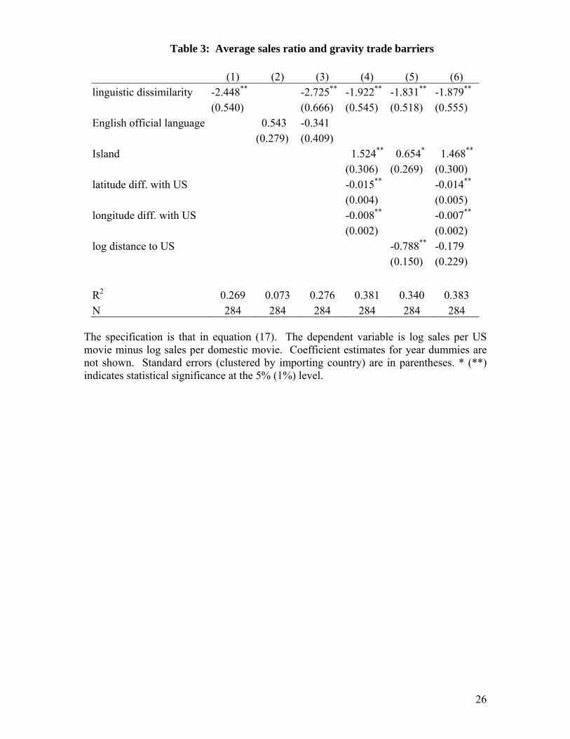
26

Table 3: Average sales ratio and gravity trade barriers

(1) (2) (3) (4) (5) (6) linguistic dissimilarity -2.448** -2.725** -1.922** -1.831** -1.879**

(0.540) (0.666) (0.545) (0.518) (0.555) English official language 0.543 -0.341 (0.279) (0.409) Island 1.524** 0.654* 1.468**

(0.306) (0.269) (0.300) latitude diff. with US -0.015** -0.014**

(0.004) (0.005) longitude diff. with US -0.008** -0.007**

(0.002) (0.002) log distance to US -0.788** -0.179 (0.150) (0.229)

R2 0.269 0.073 0.276 0.381 0.340 0.383 N 284 284 284 284 284 284

The specification is that in equation (17). The dependent variable is log sales per US movie minus log sales per domestic movie. Coefficient estimates for year dummies are not shown. Standard errors (clustered by importing country) are in parentheses. * (**) indicates statistical significance at the 5% (1%) level.

27

Table 4: Results partitioning countries by market size and distance to US Q index Q index High Low High Low (1) (2a) (2b) (3a) (3b) linguistic dissimilarity -1.922** -1.884* -2.920 -1.670* -2.587* (0.545) (0.816) (1.895) (0.625) (1.079) Island 1.524** 2.111** 1.160** 2.162** 1.073** (0.306) (0.498) (0.251) (0.519) (0.327) latitude diff. with US -0.015** -0.018** -0.013 -0.016** -0.022 (0.004) (0.007) (0.019) (0.005) (0.017) longitude diff. with US -0.008** -0.009** -0.010 -0.009** -0.006 (0.002) (0.002) (0.006) (0.002) (0.006)

R-squared 0.381 0.263 0.576 0.288 0.703 N 284 213 71 238 46

The dependent variable is log sales per US movie minus log sales per domestic movie. Column 1 shows results from the full sample (identical to column 4 of Table 3); column 2a (2b) shows results for countries with a high (low) Q index based on the partition of countries according to size and distance in Figure 7a; and column 3a (3b) shows results for countries with a high (low) Q index based on the partition of countries according to size and distance in Figure 7b. Standard errors (clustered by importing country) are in parentheses. * (**) indicates statistical significance at the 5% (1%) level.

28

Figure 1a: Pattern of Exports

Figure 1b: Increase in Global Fixed Export Cost

1u 2u …. uK , 1u K

G

Domestic movies Exported to K countries

Exported to K+1 countries …

, 2u K …

1u … uK , 1u K

G

uL , 2u K … , 1u L …

uT

'G

B = {K+1,…,T}

B’ = {L+1,…,T}

G = {1,…,K}

G’ = {1,…,L}

29

Figure 2 Constraint for Domestic Production

1bKb 1Kb

b

constraint binding constraint not binding

… 2Kb … 2b

30

Figure 3: Share of US films in national movie expenditure, 2001-2006

Figure 4: Intensive versus extensive margin of movie imports, 2001-2006

ArgentinaAus tralia

Aus tria

Belgium

Brazil

Canada

China

Czech Republic

Denmark

EstoniaFinland

France

Germ anyHungary

Iceland

Indones iaIreland

Italy

LatviaLithuania

Malays ia

Mexico

Netherlands

New Zealand

Norway

Philippines

Poland

Portugal

Rom aniaRuss ia

SingaporeSlovak Republic

Slovenia

South Korea

Spain SwedenSwitzerland Thailand

TurkeyUK

0.2

.4.6

.81

Sha

re o

f U

S in

Box

Off

ice

Rev

enue

s

0 .2 .4 .6 .8 1Share of US in No. of Films Exhibited

Lithuania

LatviaEstoniaRom aniaSlovak Republic

IcelandMalays iaSlovenia Czech Republic

PhilippinesSingapore

HungaryFinlandArgentinaThailand

Belgium

TurkeyNew ZealandPortugalIndones iaPoland

IrelandNorwayDenmarkAus triaSwedenNetherlandsSwitzerlandBrazilRuss ia

SpainItalySouth KoreaMexicoAus traliaCanada

China

FranceGerm anyUK

-4-2

02

4Lo

g nu

mbe

r of

US

film

s im

port

ed

-4 -2 0 2 4Log box-office revenues per US film

31

Figure 5: Movie imports and importing-country characteristics, 2001-2006

(a) Number of US movies imported

LithuaniaLatviaEstonia

Rom aniaSlovak RepublicIceland

Malays iaSlovenia Czech Republic

PhilippinesSingaporeHungary Finland

ArgentinaThailand

Belgium

TurkeyNew Zealand

PortugalIndones iaPolandIrelandNorwayDenmarkAus triaSwedenNetherlandsSwitzerlandBrazilRuss ia

SpainItaly

South KoreaMexicoAus traliaCanada

China

FranceGerm anyUK

-4-2

02

4Lo

g nu

mbe

r of

US

film

s im

port

ed

-4 -2 0 2 4Log GDP

Actual values Fitted values

LithuaniaLatvia Estonia

RomaniaSlovak Republic

MalaysiaSloveniaCzech Republic

PhilippinesSingaporeHungaryFinland

Argentina Thailand

Belgium

TurkeyNew Zealand

Portugal IndonesiaPoland IrelandNorwayDenmarkAustria SwedenNetherlandsSwitzerlandBrazil Russia

SpainItaly

South KoreaMexicoAustralia Canada

China

FranceGermanyUK

-4-2

02

4L

og n

um

ber

of

US

film

s im

por

ted

-.4 -.2 0 .2 .4Log linguistic dissimilarity with US

Actual values Fitted values

32

(b) Box-office revenues per US movie

LithuaniaLatviaEstonia Rom aniaSlovak Republic

Iceland Malays iaSlovenia

Czech RepublicPhilippinesSingaporeHungary FinlandArgentinaThailandBelgiumTurkeyNew ZealandPortugalIndones ia

PolandIrelandNorwayDenmarkAus triaSwedenNetherlandsSwitzerland

BrazilRuss ia

SpainItalySouth KoreaMexicoAus traliaCanada ChinaFranceGerm any

UK-4

-20

24

Log

box-

offic

e re

venu

es p

er U

S f

ilm

-4 -2 0 2 4Log GDP

Actual values Fitted values

LithuaniaLatviaEstoniaRomaniaSlovak Republic

MalaysiaSlovenia

Czech Republic PhilippinesSingaporeHungaryFinlandArgentina ThailandBelgium TurkeyNew Zealand Portugal Indonesia

Poland IrelandNorwayDenmarkAustriaSwedenNetherlandsSwitzerlandBrazil Russia

SpainItaly South KoreaMexicoAustralia Canada ChinaFranceGermany

UK

-4-2

02

4L

og b

ox-

off

ice

reve

nue

s pe

r U

S f

ilm

-.4 -.2 0 .2 .4Log linguistic dissimilarity with US

Actual values Fitted values

33

Figure 6: Relative average revenue per US movie and trade barriers, 2001-2006 (a) Distance to the US

(b) Linguistic dissimilarity with the US

Lithuania

Latvia

Estonia

Rom ania

Slovak Republic

Iceland

Malays ia

Slovenia

Czech Republic

PhilippinesSingapore

Hungary

Finland

Argentina

Thailand

Belgium

Turkey

New Zealand

Portugal

Indones ia

Poland

Ireland

NorwayDenmark

Aus tria

Sweden

Netherlands

Switzerland

Brazil

Russ iaSpain

Italy

South Korea

Mexico

Aus tralia

ChinaFrance

Germ any

UK

-2-1

01

2Lo

g re

lativ

e bo

x of

fice

reve

nue

per

film

-1 -.5 0 .5 1Log distance to US

(mean) lsd Fitted values

Lithuania

Latvia

Estonia

Rom ania

Slovak Republic

Malays ia

Slovenia

Czech Republic

PhilippinesSingapore

Hungary

Finland

Argentina

Thailand

Belgium

Turkey

New Zealand

Portugal

Indones ia

Poland

Ireland

NorwayDenmark

Aus tria

Sweden

Netherlands

Switzerland

Brazil

Russ iaSpain

Italy

South Korea

Mexico

Aus tralia

Canada

ChinaFrance

Germ any

UK

-2-1

01

2Lo

g re

lativ

e bo

x of

fice

reve

nue

per

film

-.4 -.2 0 .2 .4Log linguistic dissimilarity with US

(mean) lsd Fitted values

34

Figure 7a: Country size and linguistic distance from the US

Figure 7b: Country size and geographic distance from the US

1

0

11

1

1

00

11

111

11

0

1

1

00

1

0

1

1

000

1

0

10

1

1

00

11

1 10

1

0

1

0

0

1

1

0

1

0

1

00

0

1

0

0

0

0

1

000

0

0

00

1

00

1

00

1

10

0

00

0

00

0

0

0

0

1

0

01

11

00

0

1

1

00

0

0

0

11

11

0

0

0

00

0

1

0

0

0

000

000 0

0

0

0

0

0

0

0

0

0 0

0

010

0

1

00

0

0

10

0

0

00

00

000

0

0

1

0

0

0

0

0

00

00

0

00

0

0

1

0

0

1

00

1

1

0

0

00

0

1

0

0

0 0

0

0

1

0

0

0

0

1

0

1

0

0 00 0

1

1

00

0

000

00

0

0

00

1

0

0

0

0

0

0

0

0

1

111

0

0

0

0

00

0

1

0

0

0

000

00

0 000

0

0

1

0

000

0

0

1

000

0

0

1

00

0

00

00

0

0

0

0000

22

24

26

28

30

log

GD

P

-.8 -.6 -.4 -.2 0log linguistic dissimilarity

1

0

11

0

0

00

11

000

11

0

0

1

00

1

0

0

1

00 0

1

0

00

0

0

00

00

0 10

1

0

1

0

0

1

1

0

1

0

1

00

0

0

0

0

0

0

0

000

0

0

00

0

0 0

0

00

1

00

0

00

0

00

0

0

0

0

1

0

00

00

00

1

1

0

00

0

0

0

00

10

0

0

0

00

0

1

0

0

0

00 0

0000

0

0

0

0

0

0

0

0

0 0

0

000

0

1

00

0

0

00

0

0

00

00

000

0

0

1

0

0

0

0

0

00

00

0

00

0

0

1

0

0

1

00

1

1

0

0

00

0

0

0

0

00

0

0

1

0

1

0

0

1

0

1

0

0 000

1

1

0 0

0

0 00

00

0

0

00

1

0

0

0

0

0

0

0

0

1

111

0

0

0

0

00

0

1

1

0

0

000

00

0 000

0

0

1

0

000

0

0

1

00 0

0

0

1

00

0

00

00

0

0

0

0000

22

24

26

28

30

log

GD

P

-1 -.5 0 .5 1log geographic distance