tracking human motion with multichannel interacting multiple model

Copyright (c) 2013 IEEE. Personal use is permitted. For any other purposes, permission must be obtained from the IEEE by emailing [email protected].

This article has been accepted for publication in a future issue of this journal, but has not been fully edited. Content may change prior to final publication.

.

1

Tracking Human Motion with Multi-channel Interacting Multiple Model

Suk Jin Lee, Student Member, IEEE, Yuichi Motai, Member, IEEE, and Hongsik Choi

Abstract— Tracking human motion with multiple body sensors has the potential to promote a large number of applications such as detecting patient motion, and monitoring for home-based applications. With multiple sensors, the tracking system architecture and data processing cannot perform the expected outcomes because of the limitations of data association. For the collaborative and intelligent applications of motion tracking (Polhemus Liberty AC magnetic tracker), we propose a human motion tracking system with multi-channel interacting multiple model estimator (MC-IMME). To figure out interactive relationships among distributed sensors, we used a Gaussian mixture model (GMM) for clustering. With a collaborative grouping method based on GMM and expectation-maximization (EM) algorithm for distributed sensors, we can estimate the interactive relationship with multiple body sensors and achieve the efficient target estimation to employ a tracking relationship within a cluster. Using multiple models with filter divergence, the proposed MC-IMME can achieve the efficient estimation of the measurement and the velocity from measured datasets of human sensory data. We have newly developed MC-IMME to improve overall performance with a Markov switch probability and a proper grouping method. The experiment results shows that the prediction overshoot error can be improved in average 19.31% with employing a tracking relationship. Index Terms—motion tracking, cluster number selection, Gaussian mixture model, expectation-maximization, interacting multiple model1

I. INTRODUCTION racking human motion with multiple body sensors has the potential to improve the quality of human life and to promote a large number of application areas such as

health care, medical monitoring, and sports medicine [1-3]. Tracking human motion with multiple body sensors has a potential to promote a large number of applications of detecting patient motion and monitoring human behavior for home-based applications, e.g. smart television and gesture-based gaming. The information provided by multiple body sensors are expected to be more accurate than the information provided by a single sensor [2-4]. In multiple sensory systems, however, the tracking system architecture and data processing cannot perform the expected outcomes because of the limitations of data association [5-14]. As shown in Fig. 1, individual sensory system using IMME shows the position estimates of benign motion for the human chest. The typical problem showed in this figure is that the prediction overshoots at the beginning of tracking estimation can result in a significant prediction error. This fact has motivated us to develop an appropriate method that may reduce the initial prediction estimate error. We propose a new method to reduce the initial

1Manuscript received July 31, 2012. Revised February 20, 2013. Accepted for publication April 01, 2013. Copyright (c) 2013 IEEE. Personal use of this material is permitted. However, permission to use this material for any other purposes must be obtained from the IEEE by sending a request to [email protected] Suk Jin Lee is with the Dept. of Electrical and Computer Engineering (ECE), Virginia Commonwealth University (VCU), Richmond, VA 23284. Email: [email protected]. Yuichi Motai is with the Department of ECE, VCU, Richmond, VA 23284. Email: [email protected]. Hongsik Choi is with the Dept. of Information Technology, Georgia Gwinnett College Lawrenceville, GA 30043. Email: [email protected].

prediction estimate error by employing a tracking relationship of data association [15-25].

As a solution to prevent significant prediction overshoots from initial estimate error, we adopt multiple sensory systems with grouping method based on GMM for clustering. Clustering is a method that divides a set of distributed sensors into subsets so that distributed sensors in the subset are executed in a similar way. A variety of studies have been investigated on clustering methods based on k-means, spectral clustering, or expectation-maximization (EM) algorithm [1, 27-38]. However, a known limitation of these clustering methods is that the number of clusters must be predetermined and fixed. Recently, Bayesian nonparametric methods with Dirichlet process mixture have become popular to model the unknown density of the state and measurement noise [39-40]. But, because of the relatively small set of samples, it will not adequately reflect the characteristics of the cluster structure [30]. For the time sequential datasets of distributed body sensors, we would like to add a prior distribution on the cluster association probability [41-42]. We refer to this prior distribution as hyper-parameters [41]. Therefore, we proposed a new collaborative grouping method for distributed body sensors.

0.01 0.02 0.03 0.04 0.05 0.06 0.07 0.08 0.09 0.128

28.5

29

29.5

30

30.5

31

31.5

32

32.5

Data Time Index (Second)

Pos

ition

Est

iam

tion

valu

e (c

m)

IMMEMeasurementUpper BoundLower Bound

Prediction Overshoot

Fig. 1. Prediction Overshoot of IMME. This figure shows the position estimation of benign motion for the human chest. The upper bound and lower bound can be derived from adding the marginal value to the measurement and subtracting the marginal value from the measurement, respectively [26].

Multiple model (MM) may have multiple possible dynamic models for multi-sensor systems with Markov model switches. In such a hybrid system, the possible models make multiple sensors supply the information about the interested variable, and thus are collaborative and complementary. The basic idea of all MM approaches is that complicated target movements are made up of random variations originating from basic (straight-line) target motion. Due to the difficulty in representing this motion with a single model, MMs including potentially dynamic models operate in a parallel way with Markov switch probability [15]. The proposed solution employs a tracking relationship among distributed sensors by adding switching probability for multiple models and clustering method to figure out the interactive relation among the sensors. IMME algorithm can be used to combine different filter models with improved control of filter divergence. As a suboptimal hybrid filter [15-17], IMME makes the overall filter recursive by modifying the initial state vector and

T



.

2covariance of each filter through a probability weighted mixing of all the model states and probabilities [18-25].

The overall contribution of this paper is to minimize the prediction overshoot originating from the initialization process by newly proposed MC-IMME algorithm with the interactive tracking estimation. MC-IMME can estimate the object location as well as the velocity from measured datasets using multiple sensory channels. For this MC-IMME, we have extended the IMME to improve overall performance by adding switching probability to represent the conditional transition probability and a collaborative grouping method to select a proper group number based on the given dataset. The technical contributions of this paper are twofold: First, we propose a group number selection method for distributed body sensors based on Dirichlet hyper-prior on the cluster assignment probabilities. Second, we present a new prediction method to reduce the initial estimate error by employing a tracking relationship among distributed body sensors. For the performance improvement, we added switching probability to represent the conditional transition probability from a previous channel state to a current channel state and a collaborative transition probability to select a proper group number based on the given datasets.

This paper is organized as follows. In Section II, the theoretical background for the proposed algorithm is briefly discussed. In Sections III and IV, the proposed grouping criteria with distributed sensors placement based on EM algorithm and the proposed estimate system design for distributed body sensors are presented in detail, respectively. Section V presents and discusses experimental results of proposed methods—grouping methods and adaptive filter design. A summary of the performance of the proposed method is presented in Section VI.

II. BACKGROUND A. Kalman filter

The Kalman filter (KF) provides a general solution to the recursive minimized mean square estimation problem within the class of linear estimators [43-44]. Use of the Kalman filter will minimize the mean squared error as long as the target dynamics and the measurement noise are accurately modeled. Consider a discrete-time linear dynamic system with additive white Gaussian noise that models unpredictable disturbances. The problem formulation of dynamic and the measurement equation are as follows,

)()()()(),()()()()()1(

kwkxkHkzkvkukGkxkFkx

ii

iii

+=++=+ (1)

where x(k) is the n-dimensional state vector and u(k) is an n-dimensional known vector (which is not used in our application). The subscript i denotes quantities attributed to model Mi. v(k) and w(k) are process noise and measurement noise with the property of the zero-mean white Gaussian noise with covariance, E[v(k)v(k)T] = Q(k) and E[w(k)w(k)T] = R(k), respectively. The matrices F, G, H, Q, and R are assumed known and possibly time-varying. That means the system can be time-varying and the noise non-stationary.

The Kalman filter estimates a process by using a form of feedback control and the equations for the Kalman filter can be represented with two groups: time update equations and measurement update equations. The estimation algorithm starts with the initial estimate x̂ (0) of x(0) and associated initial covariance P(0). The problem formulation of the predicted state and the state prediction covariance can be written as:

).()()()()1(),()()(ˆ)()1(ˆ

kQkFkPkFkPkukGkxkFkx

T +=+

+=+ (2)

For the proposed MC-IMME, we use Eqs. (1) and (2) with a different model of filters, i.e., a constant velocity model and a constant acceleration model.

B. Interacting Multiple Model Framework Multiple model algorithms can be divided into three

generations: autonomous multiple models (AMM), cooperating multiple models (CMM), and variable structure multi-models (VSMM) [14-15]. The AMM algorithm uses a fixed number of motion models operating autonomously. The AMM output estimate is typically computed as a weighted average of the filter estimates. The CMM algorithm improves on AMM by allowing the individual filters to cooperate. The VSMM algorithm has a variable group of models cooperating with each other. The VSMM algorithm can add or delete models based on performance, eliminating poorly performing ones and adding candidates for improved estimation [53-54]. The well-known IMME algorithm is part of the CMM generation [15].

The main feature of the interacting multiple model (IMM) is the ability to estimate the state of a dynamic system with several behavior models. For the IMM algorithm, we have implemented two different models based on Kalman filter (KF): 1) a constant velocity (CV) filter in which we use the direct discrete-time kinematic models, and 2) a constant acceleration (CA) filter in which the third-order state equation is used [23-25, 43, 45-47]. The IMME is separated into four distinct steps: interaction, filtering, mode probability update, and combination [43]. Fig. 2 depicts a two-filter IMM estimator, where x̂ is the system state, P is the filter estimate probability, z is the measurement data, and µ are mixing probabilities. Note that the previous state of each model is reinitialized by the interaction stage each time the filter iterates. In IMME, at time k the state estimate is computed under each possible current model using CV or CA.

Fig. 2. The IMME has a four-step process in a way that different state models are combined into a single estimator to improve performance.

In Fig. 2, the mixing probability (µij) represents the conditional transition probability from state i to state j. With an initial state of each model ( ix̂ (k–1)), new filter state is computed to estimate the mixed initial condition ( ix0ˆ (k–1)) and the associated covariance (P0i(k−1)) according to the mixing probability. The above estimates and the covariance are used as input to the likelihood update matched to Mj(k), which uses the measurement data (z(k)) to yield

ix̂ (k) and Pi(k). The likelihood function corresponding to each model i (Λi) is derived from the mixed initial condition ( ix0ˆ (k–1)) and the associated covariance (P0i(k−1)). After mode probability update based on a likelihood function (Λi), combination of the model-conditioned estimates and covariance is computed for output purposes with the mixing probability. For our distributed sensory system of target estimation, each filter state of IMM is dedicated for each sensor, and distributed target estimations independently progress according to each IMME.

C. Cluster Number Selection using GMM and EM Algorithm For industrial applications of motion tracking, distributed body

sensors placed on target surface with different positions and angles can have specific correlation with others. That means distributed body sensors can cooperate with each other within a group.

)1(),1(ˆ 11 −− kPkx )1(),1(ˆ 22 −− kPkx

)1()1(ˆ 0101 −− kPkx )1()1(ˆ 0202 −− kPkx

)()(ˆ

1

1

kPkx

)()(ˆ

2

2

kPkx

( ) )(,ˆ kPkx

µ(k)

Λ1 Λ1

z(k)<Measurements>

µ(k−1)

Mode probability update and mixing probability calculation

Combination of model-conditioned estimates and covariance

<Output>

Likelihoodupdate (M1)

Likelihood update (M2)

Interaction and mixing

<CV> <CA>

Interaction

Filtering

Mode probability

update

Combination



.

3Recently, several clustering algorithms have been developed to partition the observations (L) into several subsets (G) [27-38]. The most notable approaches are a mean square error (MSE) clustering and a model-based approach. The MSE clustering typically is performed by the well-known k-means clustering. In general, k-means clustering problem is NP-hard [27], so a number of heuristic algorithms are generally used [33, 35-36].

A model-based approach to deal with the clustering problem consists of certain models, e.g., a Gaussian or a Poisson model for clusters and attempting to optimize the fit between the data and the model. The most widely used clustering method of this kind is a Gaussian mixture model (GMM) [30-32]. In GMM, the joint probability density that consists of the mixture of Gaussians φ(z; my, ∑y), where y=1...G, should be solved [29-30]. Assume a training set of independent and identically distributed points sampled from the mixture, and our task is to estimate the parameters, i.e., prior probability (αy), mean (my) and covariance (∑y) of the clustering components (G) that maximize the log-likelihood function δ(⋅) based on EM algorithm [30, 32]. Given an initial estimation (α0, m0, ∑0), EM algorithm calculates the posterior probability p(y|zj) in E-step. Based on the estimated result we can calculate the prior probability (αy), mean (my) and covariance (∑y) for the next iteration, respectively, in the following M-step [48-50].

The log-likelihood for the incomplete datasets in the EM algorithm can never be decreased (see Chapter 1.6 in [51]), because the EM algorithm iterates the computations E-step and M-step until the convergence to a local maximum of the likelihood function. That means that the consecutive log-likelihood functions monotonically increase and could be very similar but not identical. We define the discrepancy of consecutive values as the difference (∆). Now, we can define the difference (∆) as follows:

)1,(),()( −Θ−Θ≅∆ GGG δδ . (3) Once we estimate the parameter Θ ≡ {αy, my, ∑y}G

y=1 we can find the optimal cluster number (G*) with the conventional Brute-force search algorithm by introducing ∆(G) that is a log-likelihood function after parameter learning with the following equation: G* = argming∆(G). In practice, we can set a threshold (∆th) that is almost closed to zero to save the redundant iteration step. We can start with G = 2 for a first candidate solution for cluster number selection, estimate the set of finite mixture model parameter Θ* ≡ {α*

y, m*y, ∑*

y}Gy=1 using EM algorithms based on the sample

data, and calculate ∆(G). After checking whether a candidate G is an appropriate cluster number for L, we can use the cluster number G as an appropriate cluster. The search algorithm based on the log-likelihood function can only work in the static data model, but cannot guarantee to work in the time sequential data because of the lack of adaptive parameter for the time sequential data. Thus, it has the following two limitations: 1) it can only work within limitation of the initial dataset, and 2) it cannot guarantee the global optimal based on the time sequential data because of the lack of adaptive parameter for the time sequential data. To overcome such static grouping limitations, we introduce distributed grouping using the multi-channel (MC) selection for the time sequence data of distributed body sensors in the next subsection.

III. PROPOSED GROUPING CRITERIA WITH DISTIBUTED SENSORS The motivation of this section is to prepare interactive

relationships among distributed sensory data for clustering, i.e., how to collaborate with distributed measurements to achieve better performances compared to the single measurement. In Section III.A, we will show how to initialize the hyper-parameter presenting a hypothetical prior probability for background knowledge, and can select the collaborative cluster number using EM iteration. In Section III.B, we will calculate switching

probability representing the conditional transition probability from channel a to channel b within a cluster number. A. Collaborative Grouping with Distributed Body Sensors

The cluster number selection using GMM works well in the distributed means model as well as in the static data model. But it only works within limitation of the initial dataset. The tracking estimate system with distributed body sensors has time sequential data. That means the measured information from each sensor can be changed depending on the applications from time to time. To make the collaborative grouping system, we introduce some background knowledge that can be presented as a hypothetical prior probability (βy) that we call hyper-parameter [41-42]. Suppose that αy(k) is an initial prior probability at time k. The initial hyper-parameter βy can be found as follows:

)(lim)0( kyky αβ∞→

= (4)

In practice, we can get the hyper-parameter (βy) using sample training data instead of the infinite training data with respect to time. After calculating the hyper-parameter with sample training data using (4), the hyper-parameter (βy) should be adaptive with respect to time k. Please note that the hyper-parameter can be selected based on the global information of sample data. This parameter is selected for corresponding to the steady state. It can be accomplished using the switching probability that will be explained in detail in Section IV.C. The adaptive hyper-parameter can be increased or decreased based on the current switching probability comparing to the previous switching probability, and can be calculated as follows:

,)1()( yyy kk µββ ∆+−= (5)

where ∆µy is the difference between the current switching probability and the previous one. ∆µy can be calculated using a switching probability at time k, i.e., µy(k) indicating the switching weight of group y. We will describe how to select the difference (∆µy) in detail in Section IV.D. After calculating the adaptive hyper-parameter, the adaptive (ADT) posterior probability pADT(y|zj) is calculated at time k in E-step as follows:

∑∑==

+∑

+∑= G

yy

G

y

ty

tyj

ty

yt

yt

yjt

yjADT

kmz

kmzkzyp

11

)()()(

)()()(

)(),;(

)(),;())(|(

βφα

βφα (6)

Using the modified one, we can proceed to the M-step at time k as follows:

[ ]∑

∑∑

∑

∑

=

+++

=

=

=+

=

+

−−=∑

==

=

L

j

Ttyj

tyjjADT

y

ty

L

jjjADT

yL

jjADT

L

jjjADT

ty

L

jjADT

ty

mzmzzypL

k

zzypLzyp

zzypkm

kzypL

k

1

)1()1()1(

1

1

1)1(

1

)1(

))(()|(1)(

,)|(1

)|(

)|()(

,))(|(1)(

α

α

α (7)

We can estimate the tth iteration result of the adaptive posterior probability pADT(y|zj) at time k from (6). Based on the modified result we can calculate the prior probability (αy), the mean (my), and the covariance (∑y) in the (t+1)th iteration for the collaborative grouping for time sequential data, respectively, using (7). A local maximum at time k can be selected by iterating the above two steps. We can select the collaborative cluster number (G*ADT) by introducing ∆ADT(G) that is a log-likelihood function after parameter learning with the following equations:

)1,(),()(

),(minarg**

*

−Θ−Θ=∆

∆=

GGG

GG

ADTADTADT

ADTG

ADT

δδ (8)

where δADT is a log-likelihood function with the adaptive posterior probability. Note that Eq. (3) is extended into Eq. (8) with the hyper-parameter (βy). Comparing with the previous algorithm, the collaborative grouping with time sequential data



.

4can select local maxima at time k by iterating two steps: E-step and M-step. We can select the global optimal from a series of local maxima of time k. B. Estimated Parameters used for IMME

Collaborative grouping with time sequence data can select local maxima at time k using the difference (∆) of the consecutive log-likelihood functions. We can set the difference (∆) of the consecutive log-likelihood functions as ∆(G*, k) with respect to time k. To reduce the notation complexity, ∆(k) is simply used for ∆(G*, k). Now we can use this ∆(k) for IMME to estimate the multi-channel estimates and covariance. As mentioned, the log-likelihood function in each EM step cannot decrease [51]. That means we can minimize the difference (∆(k)) of the consecutive log-likelihood functions with respect to time k because ∆(k) converges to zero over a period of time. Therefore, we can find out the following relationship: ∆(k−1) ≥ ∆(k). In the standard IMME, it is assumed that the mixing probability density is a normal distribution all the time. Now we derive the switching probability (µab) for the estimated parameter from mixing probability (µij). Since it is hard to get µab(k-1) directly, we used a tractable estimation µab(k-1)+∆(k-1), as follows:

)1()1()1( −∆+−=− kkk ijab µµ , (9) where µij is the mixing probability that represents the conditional transition probability from state i to state j, and µab is the switching probability that represents the conditional transition probability from channel a to channel b. Note that we define mixing probability (µij) as switching probability (µab). That means our assumption is still valid in the switching probability, i.e., switching probability density follows a normal distribution. The equality of Eq. (9) is true because the value of ∆(k-1) can be zero as k goes to the infinity. We can use the right side of Eq. (9) to dynamically select the switching probability (µab) with ∆(k). Eq. (9) above provides us with a method to design the filter for distributed sensors at the second stage, because the switching probability can be adjusted more dynamically based on ∆(k) in the second stage filter. We will explain how to estimate the MC estimates and covariance using (9) in the next section.

IV. MULTI-CHANNEL (MC) IMME: PROPOSED SYSTEM DESIGN The proposed method with collaborative grouping for

distributed sensory data can achieve the efficient target estimation by using geometric relationships of target information emerging from distributed measurements. Fig. 3 shows a general block diagram to represent the relationship between the proposed method (MC-IMME) and IMME.

Fig. 3. General block diagram for the proposed MC-IMME.

In MC-IMME, grouping data can be used for target-tracking estimation with IMME. Geometric information of distributed measurements is used for the switching probability update in the target estimation. Even though the proposed method needs the initialization process that is the same as in the IMME prediction, the interactive relationship with distributed sensors can compensate for the prediction estimate error. For the interactive tracking estimate, the proposed system design herein can be extended from Fig. 2 to Fig. 4. A. MC Mixed initial condition and the associated covariance

Starting with an initial yax (k–1) for each channel a in a group y,

new filter state is computed to estimate the mixed initial condition

and Kalman filter covariance matrices (10) according to the relationships

( ) ( ) ( )

( ) ( )∑

∑

=

=

−+−−=−

−−=−

r

a

yab

ya

yab

ya

r

a

yab

ya

ya

kDPkPkkP

kkxkx

1

0

1

0

)]1()1(][1[1

,]1[11ˆ

µ

µ (10)

where yabµ is a switching probability presenting the relationship

between channel a and channel b within the same group y. As shown in Fig. 4, we have added the blue line indicating how the difference (∆(k)) in Stage 1 would be used for Stage 2. We denote r as the channel number of the group and DPab

y(k-1) as an increment to the covariance matrix to account for the difference in the state estimates from channels a and b, expressed by [ y

ax (k–1) – ybx (k–1|)]⋅[ y

ax (k–1) – y

bx (k–1)]T. Note that the initial states of IMME are extended into Eq. (10)

incorporating with the switching probability and ∆(k–1). We have adopted the results of Section III on grouping criteria ∆(k) of Eq. (9). The difference (∆(k)) can be minimized with respect to time k, so we can adjust to estimate the filter state from a coarse probability to a dense probability.

B. MC Likelihood Update The above estimates and covariance are used as input to the

filter matched to May(k), which uses za

y(k) to yield yax̂ (k) and

yaP (k). The likelihood functions corresponding to each channel

are computed using the mixed initial condition and the associated covariance matrix (10) as follows: Λa

y(k)=p[z(k)| May(k),

yax 0ˆ (k−1), y

aP 0 (k−1)], where y is a group number and r(y) is the number of sensors for each group y. To reduce the notation complexity, r is simply used for r(y).

C. Switching Probability Update Given the likelihood function (Λa

y(k)) corresponding to each channel, the switching probability update is done as follows:

,,1,,...,1,)(1)(11∑∑==

Λ=Λ=Λ=Λ=G

yy

yy

r

a

ya

yy

y

y

y ccr

Gyckc

kµ (11)

where Λy is the likelihood function for a group y, cy is the summarized normalization constant, r is the channel number of a group y, and G is the number of group. Eq. (11) above provides the probability matrices used for combination of MC-conditioned estimates and covariance in the next step. It can also show us how to use these parameter results for collaborative grouping criteria with multiple sensors. D. Feedback from Switching Probability Update to Stage 1 for

Grouping Criteria with Distributed Sensors For the collaborative grouping, we introduced the adaptive

hyper-parameter (βy(k)) in Section III.A. The adaptive hyper-parameter βy(k) can be dynamically increased or decreased depending on the weight of the channel. The weight of channel can be represented as the switching probability. That means we can use the switching probability (µy(k)) as a reference to adjust the adaptive hyper-parameter as follows:

.)1()()1()()1()()1()()1()()1()(

−<−<−=−=−>−>

kkifkkkkifkkkkifkk

yyyy

yyyy

yyyy

µµββµµββµµββ

(12)

If there is no change of the switching probability, βy(k) is the same as βy(k–1). If the current switching probability is greater than the previous one, βy(k) could be increased; otherwise, βy(k) could be decreased as shown in (12). Therefore, we can calculate the difference (∆µy) between the current switching probability and the previous one as follows:

< IMME > < Grouping Measurement data

Grouping data

Geometric relationships

Switching probability

Target estimation



.

5

z1

z2

z3

z4

Sensor 1

Sensor 2

Sensor 3

Sensor 4

<y1>α1, β1

φ(z; m1, ∑1)

<yn`>αn, βn

φ(z; mn, ∑n)

z11

z12

Likelihood update (M11) (Sec IV.B)


Switching probabilityupdate (Sec IV.C)

Combination ofMC conditionedestimates and

covariance(Sec IV.E)

Multiple-channel mixed initial conditionand the associated covariance (Sec IV.A)

• • • • • • • • •

< Stage 1 > < Stage 2 >

)13.(

1

Eqµ∆

∆(k)

∆(k)

Forward from Stage 1 to Stage 2

Feedback from Stage 2 to Stage 1

( ) ( ))10.(

011

011 1,1ˆ

EqkPkx −−

( ) ( ))10.(

012

012 1,1ˆ

EqkPkx −−

)(11 kΛ

)(12 kΛ

( ))11.(

1

Eqkµ

( ) ( )kPkx 11

11 ,

( ) ( )kPkx 12

12 ,

( ) ( ))14.(

11

11 ,ˆ

EqkPkx

( ) ( ))14.(

12

12 ,ˆ

EqkPkx

( ))11.(

1

Eqkµz1

z2

z3

z4

Sensor 1

Sensor 2

Sensor 3

Sensor 4

<y1>α1, β1

φ(z; m1, ∑1)

<yn`>αn, βn

φ(z; mn, ∑n)

z11

z12



Switching probabilityupdate (Sec IV.C)

Combination ofMC conditionedestimates and

covariance(Sec IV.E)

Multiple-channel mixed initial conditionand the associated covariance (Sec IV.A)

• • • • • • • • •

< Stage 1 > < Stage 2 >

)13.(

1

Eqµ∆

∆(k)

∆(k)

Forward from Stage 1 to Stage 2

Feedback from Stage 2 to Stage 1

( ) ( ))10.(

011

011 1,1ˆ

EqkPkx −−

( ) ( ))10.(

012

012 1,1ˆ

EqkPkx −−

)(11 kΛ

)(12 kΛ

( ))11.(

1

Eqkµ

( ) ( )kPkx 11

11 ,

( ) ( )kPkx 12

12 ,

( ) ( ))14.(

11

11 ,ˆ

EqkPkx

( ) ( ))14.(

12

12 ,ˆ

EqkPkx

( ))11.(

1

Eqkµ

Fig. 4. System design for distributed body sensors has two stages. At the first stage, all the distributed sensors are partitioned into the groups that have a tracking relationship with each other. At the second stage, the interactive tracking estimate is performed for distributed groups.

)1()( −−=∆ kk yyy µµµ (13) That means the adaptive hyper-parameter βy(k) can be

increased or decreased based on the current switching probability compared to the previous one. In Fig. 4, we have added the red line indicating how the difference of the switching probability in Stage 2 would be used for Stage 1.

E. Combination of MC conditioned estimates and covariance Combination of the MC conditioned estimates and

covariance is done according to the mixture equations

.)]()()][([)(

,)]()[()(ˆ

1

1

∑

∑

=

=

+=

=

r

b

yb

yb

yab

ya

r

b

yab

yb

ya

kDPkPkkP

kkxkx

µ

µ (14)

where yabµ is a switching probability presenting the

relationship between channel a and channel b within the same group y, and DPb

y(k) as an increment to the covariance matrix to account for the difference between the intermediate state and the state estimate from model b, expressed by [ y

bx (k) – ybx̂ (k)]⋅[ y

bx (k) – ( ybx̂ (k)]T.

Note that the combination of the model-conditioned estimates and covariance matrices in Fig. 2 is extended into Eq. (14) incorporating with the switching probability and ∆(k). As can be seen in Section IV.A, we also have adopted the results of Section III on grouping criteria ∆(k) of Eq. (9). In Fig. 4, the entire flow chart illustrates the idea of MC-IMME proposed in this study. We have added the blue line indicating how the difference (∆(k)) in Stage 1 would be used for the IMME outcomes of Stage 2, corresponding to (14). This combination is only for output purposes. F. Computational Time

We have evaluated how much additional computational time is required when we implement the proposed method by comparing it to the standard KF and the IMME method in Table I.

TABLE I COMPARISON OF THE COMPUTATIONAL COMPLEXITY Methods KF IMME MC-IMME

Complexity O(L×k×N 3) O(L×k×T(N) O(L×k×T(N)

The computational complexity of the standard KF for the upper bound is orders of growth N3, where N represents the states estimated using KF derived by Karlsson et al. [44]. The computational complexity can be increased as a linear function

of the sensor number (L) and time k. Accordingly, the asymptotic upper bound of KF is orders of growth L×k×N3.

IMME extends the complexity by defining T(N) as the asymptotic upper bound of recursive computation based on the states estimated using IMME. In the IMME the computational complexity is increased as a linear function of the independent sensor number (L). In addition, IMME needs recursive computation based on time k. Therefore, the asymptotic upper bound for the worst-case running time of IMME is orders of growth L×k×T(N) [52].

Let us define T(L) as a upper bound of iteration execution time for k-means clustering based on L points. Har-Peled et al. showed that the k-means heuristic needs orders of growth L iterations for L points in the worst case [35]. In addition, the adaptive grouping method needs to calculate the difference (∆ADT(G)) of the consecutive log-likelihood functions based on time sequential data (k) for the appropriate group number selection. Therefore, the upper bound for the worst-case running time of the adaptive grouping method is orders of growth L×k×T(L).

MC-IMME uses the same recursive computation as IMME with respect to the estimate states. That means the running time of stage 2 is the same as IMME. MC-IMME also needs additional computation for the first stage to make grouping. Suppose that asymptotic upper bound of recursive computation (T(N)) is equal to a upper bound of iteration execution time for k-means clustering (T(L)). Then, the asymptotic upper bound for the computational complexity of Multiple-channel is orders of growth L×k×T(N), because both stage 1 and stage 2 have the same orders of growth L×k [52]. Please note that IMME and MC-IMME have the identical computational complexity since distributed sensory systems both have the same channel number L, and the same data length k.

V. EXPERIMENTAL RESULTS The motivation of this section is to validate the proposed

MC-IMME with comprehensive experimental results. In Section V.A, we will describe the target motions for the experimental tests (chest, head, and upper body). For each target motion, the optimal cluster number based on the proposed grouping method is selected follows in Section V.B, and this selection number is further investigated in comparison to grouping number methods using other clustering techniques in Section V.C. The prediction accuracy of the proposed MC-IMME is evaluated with the normalized root mean squared error (NRMSE) and the prediction overshoots, in Section V.D and V.E, respectively. We also show CPU time used for the computational time in Section V.F.



.

6A. Motion Data

We have used three kinds of motion data, i.e., chest motion, head motion, and upper body motion. Motion data was collected using a Polhemus Liberty AC magnetic, operating at 240Hz for approximately 20 seconds and 100 seconds [55]. Eight sensors were attached on the target motion surface with the magnetic source rigidly mounted approximately 25.4 cm from the sensors. Each motion data was randomly selected based on the motion speed for Monte Carlo analysis with four sets of motion data—the first datasets for slow motion, the second datasets for moderate, the third for the violent motion, and the fourth for the complex motion including slow, moderate, and violent motions. For the target estimation, the experimental tests have been conducted based on repeated random sampling to compute their results for Monte Carlo analysis. Each of the datasets was taken with great care to limit target movement to the type based on Table II.

TABLE II CHARACTERISTICS OF MOTION DATA WITH SHORT LENGTH AND LONG LENTH

Motion Data Motion Type Speed (cm/sec) Recording Time (sec)

Chest_S Slow motion 0.64 − 0.87 20.72

Chest_M Moderate motion 6.70 − 7.91 20.40

Chest_V Violent motion 24.84 − 32.63 22.18

Chest_C Complex motion 1.46 – 32.54 105.8

Head_S Slow motion 0.63 − 1.08 20.36

Head_M Moderate motion 6.62 − 8.37 20.40

Head_V Violent motion 16.07 − 67.70 21.43

Head_C Complex motion 1.08 – 66.16 104.05

Upper Body_S Slow motion 0.68 − 1.48 20.83

Upper Body_M Moderate motion 3.64 − 28.08 20.64

Upper Body_V Violent motion 38.48 − 118.18 21.03

Upper Body _C Complex motion 1.36 – 117.98 104.15

B. Collaborative Grouping Initialization

Before the efficient target tracking, the proposed collaborative method needs to make the grouping for distributed sensory data. The objective of this section is to find out the optimal group number with an adaptive hyper-parameter. First, we need to find out the initial hyper-parameter (βy) in Section V.B.1 and then calculate the group number (G) based on the adaptive (ADT) posterior probability pADT(y | zj). Section V.B.2 and Section V.B.3 compared the difference (∆) of the consecutive log-likelihood functions between non-collaborative grouping method described in Section II.B and collaborative grouping method described in Section III.A.

1) Calculation of hyper-parameter (βy)

2 3 4 5 6 70

0.5

Group number (G)

β y Chest

β1 β2 β3 β4 β5 β6 β7

2 3 4 5 6 70

0.5 Head

Group number (G)

β y

2 3 4 5 6 70

0.5 Upper Body

Group number (G)

β y

Fig. 5. Hyper-parameter values based on the motion data and group number.

The objective of this section is to calculate the initial hyper-parameter (βy) with potential group numbers. To find out the hyper-parameter, we iterate expectation and maximization steps with sample training data (approximately 2,400 sample dataset) for each motion. We increased the group number (G) of EM process from two to seven to show all the potential hyper-parameters. Please note that we have eight sensory channels, so that we can show all available group numbers.

Fig. 5 shows the hyper-parameters (βy, where y is a group number) described in Eq. (4), based on the target motion data and group number (G). Given in Fig. 5, we can notice that the higher the group number, the bigger the iteration number; and the more even the group distribution probabilities of a sample training data, the smaller the iteration number.

2) Calculation of the difference (∆) of the consecutive log-likelihood with non-collaborative grouping

The objective of this section is to find an optimal cluster number (G*) with the consecutive log-likelihood functions (3) based on EM process. Fig. 6 below shows the difference (∆(G)) of the consecutive log-likelihood functions, described in Eq. (3). For example, when G=2, we calculate all the log-likelihood functions of EM operations, and then select the minimum as a representing value in Fig. 6. We iterate the same procedure with different group number (G =2,..., 7) in the three kinds of the motion data. We expect to find out, as described in Section II.B, the minimum of ∆(G).

1 2 3 4 5 6 70

500

1000

1500

2000

2500

3000

Group Number (G)

Diff

eren

ce ( ∆

(G))

ChestHeadUpper Body

Fig. 6. The difference (∆(G)) of the consecutive log-likelihood with non-collaborative grouping.

Given the results in Fig. 6, we may select the group number G* for the three datasets: 2, 4, or 6 for Chest; 2 or 3 for Head; and 2, 4, 5, or 6 for Upper Body. As the group numbers are increased, the differences start to become drastically greater.

However, we cannot identify the least minimum number; for example, it is hard to choose among 2, 4, 5, or 6 for Upper Body. Therefore, in the next experiment, we will recalculate the difference (∆ADT(G)) of the consecutive log-likelihood with collaborative grouping.

3) Calculation of the difference (∆) of the consecutive log-likelihood with collaborative grouping

The objective of this section is to find an optimal cluster number (G*) using log-likelihood function with the adaptive posterior probability (8). Based on the initial hyper-parameter (βy) of Section V.B.1), we can calculate the adaptive (ADT) posterior probability pADT(y | zj) and iterate E-step (6) and M-step (7) with a specific group number (G).

Now we can show the difference (∆ADT(G)) of the consecutive log-likelihood functions, described in Eq. (8) of Section III.A, with the adaptive posterior probability in the three kinds of the motion data. We applied Eq. (8) for the



.

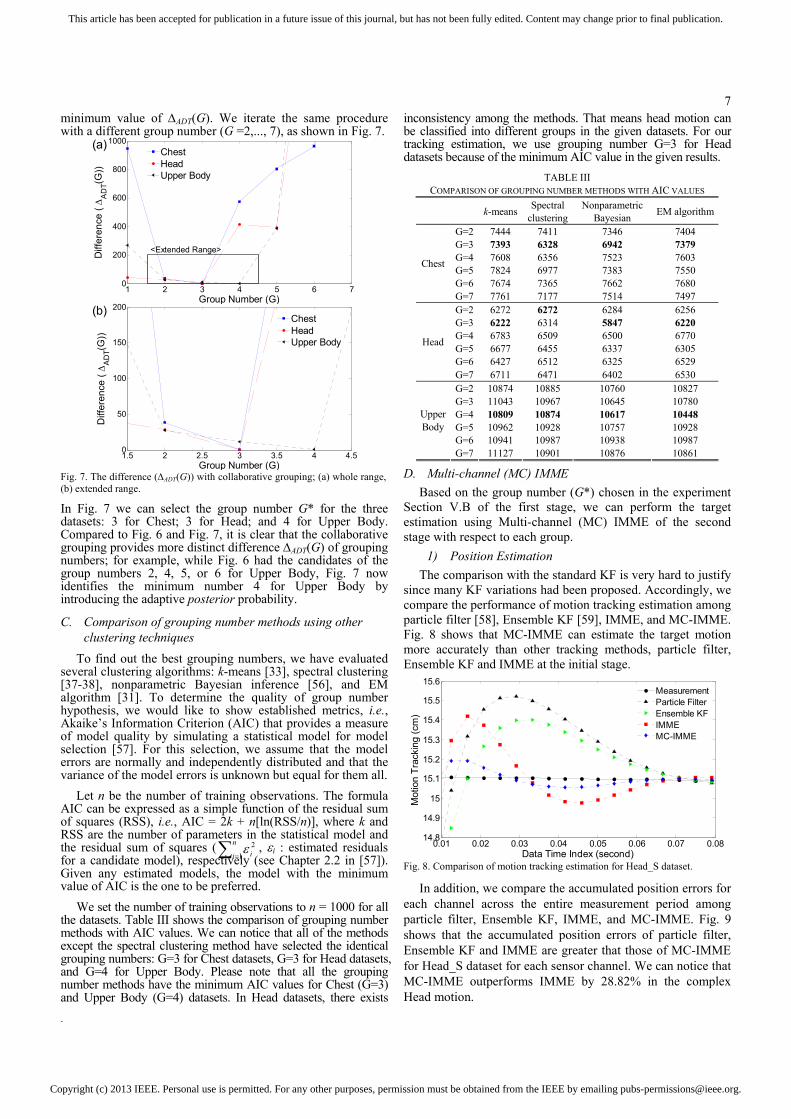
7minimum value of ∆ADT(G). We iterate the same procedure with a different group number (G =2,..., 7), as shown in Fig. 7.

1 2 3 4 5 6 70

200

400

600

800

1000

Group Number (G)

Diff

eren

ce ( ∆

AD

T(G))

ChestHeadUpper Body

(a)

<Extended Range>

1.5 2 2.5 3 3.5 4 4.50

50

100

150

200

Group Number (G)

Diff

eren

ce ( ∆

AD

T(G))

ChestHeadUpper Body

(b)

Fig. 7. The difference (∆ADT(G)) with collaborative grouping; (a) whole range, (b) extended range.

In Fig. 7 we can select the group number G* for the three datasets: 3 for Chest; 3 for Head; and 4 for Upper Body. Compared to Fig. 6 and Fig. 7, it is clear that the collaborative grouping provides more distinct difference ∆ADT(G) of grouping numbers; for example, while Fig. 6 had the candidates of the group numbers 2, 4, 5, or 6 for Upper Body, Fig. 7 now identifies the minimum number 4 for Upper Body by introducing the adaptive posterior probability.

C. Comparison of grouping number methods using other clustering techniques

To find out the best grouping numbers, we have evaluated several clustering algorithms: k-means [33], spectral clustering [37-38], nonparametric Bayesian inference [56], and EM algorithm [31]. To determine the quality of group number hypothesis, we would like to show established metrics, i.e., Akaike’s Information Criterion (AIC) that provides a measure of model quality by simulating a statistical model for model selection [57]. For this selection, we assume that the model errors are normally and independently distributed and that the variance of the model errors is unknown but equal for them all.

Let n be the number of training observations. The formula AIC can be expressed as a simple function of the residual sum of squares (RSS), i.e., AIC = 2k + n[ln(RSS/n)], where k and RSS are the number of parameters in the statistical model and the residual sum of squares (∑=

n

i i12ε , εi : estimated residuals

for a candidate model), respectively (see Chapter 2.2 in [57]). Given any estimated models, the model with the minimum value of AIC is the one to be preferred.

We set the number of training observations to n = 1000 for all the datasets. Table III shows the comparison of grouping number methods with AIC values. We can notice that all of the methods except the spectral clustering method have selected the identical grouping numbers: G=3 for Chest datasets, G=3 for Head datasets, and G=4 for Upper Body. Please note that all the grouping number methods have the minimum AIC values for Chest (G=3) and Upper Body (G=4) datasets. In Head datasets, there exists

inconsistency among the methods. That means head motion can be classified into different groups in the given datasets. For our tracking estimation, we use grouping number G=3 for Head datasets because of the minimum AIC value in the given results.

TABLE III COMPARISON OF GROUPING NUMBER METHODS WITH AIC VALUES

k-means Spectral clustering

Nonparametric Bayesian EM algorithm

G=2 7444 7411 7346 7404 G=3 7393 6328 6942 7379 G=4 7608 6356 7523 7603 G=5 7824 6977 7383 7550 G=6 7674 7365 7662 7680

Chest

G=7 7761 7177 7514 7497 G=2 6272 6272 6284 6256 G=3 6222 6314 5847 6220 G=4 6783 6509 6500 6770 G=5 6677 6455 6337 6305 G=6 6427 6512 6325 6529

Head

G=7 6711 6471 6402 6530 G=2 10874 10885 10760 10827 G=3 11043 10967 10645 10780 G=4 10809 10874 10617 10448 G=5 10962 10928 10757 10928 G=6 10941 10987 10938 10987

UpperBody

G=7 11127 10901 10876 10861

D. Multi-channel (MC) IMME Based on the group number (G*) chosen in the experiment

Section V.B of the first stage, we can perform the target estimation using Multi-channel (MC) IMME of the second stage with respect to each group.

1) Position Estimation The comparison with the standard KF is very hard to justify

since many KF variations had been proposed. Accordingly, we compare the performance of motion tracking estimation among particle filter [58], Ensemble KF [59], IMME, and MC-IMME. Fig. 8 shows that MC-IMME can estimate the target motion more accurately than other tracking methods, particle filter, Ensemble KF and IMME at the initial stage.

0.01 0.02 0.03 0.04 0.05 0.06 0.07 0.0814.8

14.9

15

15.1

15.2

15.3

15.4

15.5

15.6

Data Time Index (second)

Mot

ion

Trac

king

(cm

)

MeasurementParticle FilterEnsemble KFIMMEMC-IMME

Fig. 8. Comparison of motion tracking estimation for Head_S dataset.

In addition, we compare the accumulated position errors for each channel across the entire measurement period among particle filter, Ensemble KF, IMME, and MC-IMME. Fig. 9 shows that the accumulated position errors of particle filter, Ensemble KF and IMME are greater that those of MC-IMME for Head_S dataset for each sensor channel. We can notice that MC-IMME outperforms IMME by 28.82% in the complex Head motion.



.

8TABLE IV

OVERALL PERFORMANCE OF ACCUMULATED ERROR AMONG THE DATASETS LISTED IN TABLE II Chest_S Chest_M Chest_V Chest_C Head_S Head_M Head_V Head_C Body_S Body_M Body_V Body_C

Min. 4.79 14.96 56.92 148.67 8.20 9.28 13.97 55.06 10.92 11.94 120.45 279.50Avg. 5.19 16.20 46.25 130.28 9.00 10.51 49.81 130.01 13.38 39.42 200.26 498.58PF Max. 6.12 17.47 38.53 118.12 9.76 11.43 130.14 294.95 16.31 125.48 636.21 1549.62Min. 3.84 12.51 35.87 101.86 4.78 5.86 11.92 42.53 3.42 6.06 40.87 53.12 Avg. 4.24 13.75 43.59 119.02 5.58 7.09 47.76 116.95 5.88 31.98 192.69 459.23EnKF Max. 5.17 15.03 54.26 144.19 6.34 8.00 128.08 283.61 8.81 118.05 543.79 1339.41Min. 2.92 6.53 15.97 45.89 2.49 2.32 9.28 25.83 2.63 3.67 21.64 51.26 Avg. 3.67 11.54 18.19 63.72 6.98 7.32 23.25 86.34 6.59 50.45 166.13 467.86IMME Max. 5.75 14.29 21.58 78.91 10.12 9.78 92.51 248.99 9.75 120.24 261.89 847.67Min. 2.14 3.26 8.43 25.51 1.87 1.84 5.54 12.69 1.13 1.18 9.17 25.55 Avg. 2.73 6.87 10.95 40.44 3.29 4.38 21.19 61.46 3.79 24.75 108.87 352.93MC-

IMME Max. 3.87 10.31 12.39 48.44 4.19 6.12 51.16 134.33 7.89 87.95 181.78 623.37(Unit: Accumulated error (cm))

TABLE V ERROR PERFORMANCE AMONG PREDICTION TIME HORIZON

Window Chest_S Chest_M Chest_V Chest_C Head_S Head_M Head_V Head_C Body_S Body_M Body_V Body_C100ms 0.102 0.229 0.449 0.302 0.129 0.215 0.649 0.387 0.057 0.196 0.958 0.489 200ms 0.190 0.521 0.508 0.469 0.189 0.491 0.688 0.521 0.092 0.300 1.000 0.557 300ms 0.274 0.590 0.498 0.504 0.239 0.551 0.763 0.586 0.123 0.386 1.022 0.598 PF

400ms 0.338 0.623 0.529 0.548 0.285 0.582 0.695 0.592 0.149 0.504 0.963 0.631 100ms 0.086 0.153 0.412 0.251 0.119 0.143 0.596 0.334 0.051 0.171 0.898 0.451 200ms 0.151 0.472 0.467 0.417 0.173 0.446 0.631 0.476 0.080 0.263 0.932 0.514 300ms 0.231 0.544 0.459 0.461 0.217 0.505 0.708 0.535 0.107 0.327 0.944 0.553 EnKF

400ms 0.294 0.567 0.479 0.491 0.255 0.533 0.646 0.578 0.128 0.431 0.892 0.575 100ms 0.081 0.127 0.400 0.243 0.116 0.119 0.579 0.342 0.049 0.163 0.878 0.442 200ms 0.138 0.455 0.454 0.405 0.168 0.431 0.612 0.485 0.076 0.250 0.909 0.497 300ms 0.216 0.528 0.446 0.451 0.209 0.489 0.690 0.531 0.102 0.307 0.918 0.521 IMME

400ms 0.280 0.549 0.463 0.473 0.245 0.516 0.629 0.570 0.121 0.407 0.869 0.553 100ms 0.028 0.102 0.335 0.218 0.025 0.092 0.511 0.264 0.014 0.146 0.796 0.398 200ms 0.085 0.440 0.452 0.397 0.043 0.425 0.607 0.462 0.033 0.235 0.898 0.476 300ms 0.167 0.505 0.443 0.435 0.059 0.481 0.684 0.504 0.057 0.291 0.900 0.504

MC-IMME

400ms 0.230 0.517 0.457 0.451 0.075 0.504 0.623 0.546 0.073 0.391 0.842 0.538 (Unit: NRMSE value)

1 2 3 4 5 6 7 80

2

4

6

8

10

12

14

Sensor Number

Accu

mul

ated

Pos

ition

Erro

r (cm

)

Particle Filter Ensemble KF IMME MC-IMME

Fig. 9. Comparison of accumulated position error of each channel for Head_S.

Table IV shows the overall performance of accumulated error among the datasets listed in Table II. As shown in Table IV, MC-IMME can show the improvement with comparison to particle filter and Ensemble KF. In addition, the proposed method outperforms IMME around by 25.61~40.47% in the chest motion, 8.86~52.87% in the head motion, and 42.94~ 50.94% in the aggressive motion. Please note that the proposed method can achieve 50.94% improvement over IMME in the upper body motion.

2) Prediction Time Horizon For the prediction accuracy, we changed the prediction time horizon. Here, prediction time horizon is the term to represent the time interval window to predict the future sensory signal. We would like to compare the error performance with the various prediction time horizons among particle filter, Ensemble KF, IMME, and MC-IMME in Table V. For the comparison, we used a normalization that is the normalized

root mean squared error (NRMSE) between the predicted and actual signal over all the samples in the test datasets.

In Table V, the prediction accuracy of Chest_S dataset in the proposed MC-IMME was improved by 49.67% for particle filter, 40.16% for Ensemble KF, and 36.10% for IMME of the average prediction time horizon. We can notice that the proposed method outperforms particle filter, Ensemble KF and IMME in the other Chest motion datasets as well, even though the average improvements were less than 17% with comparison to IMME. The average improvements were 28.14% for particle file, 18.55% for Ensemble KF, and 14.46% for IMME.

In the Head_S dataset, the prediction accuracy was significantly improved by 76.73% for particle filter, 74.39% for Ensemble KF, and 73.50% for IMME of the average prediction time horizon. Notice that the improvement of prediction accuracy for the proposed method maintained around 15% across the prediction time horizons. In the other Head motion datasets, the proposed method can improve other methods, even though the average improvements were less than 5% in comparison to IMME. The average improvements were 33.93% for particle filter, 26.61% for Ensemble KF, and 23.54% for IMME.

In the Upper_Body_S dataset, the prediction accuracy of the proposed method was improved by 61.12% for particle filter, 55.30% for Ensemble KF and 52.95% for IMME of the average prediction time horizon. We can notice that the improvement of MC-IMME maintained around 40% across the prediction time horizons. We can also notice that the proposed method outperforms particle filter for 28.72%, Ensemble KF for 20.54%, and IMME for 17.33% of the average prediction time horizon over all the datasets, even though the average improvements were less than 6.39% for Upper_Body_M, 3.90% for Upper_Body_V, and 6.09 for Upper_Body_C in comparison to IMME.



.

93) Effect of the feedback/forward method

We would like to show the advantage of the proposed feedback/forward method by comparing the performance of velocity estimation of MC-IMME with no feedback/forward vs. feedback/forward. We have evaluated the tracking performance of the average velocity for the Chest_V dataset in Fig. 10. We have observed that the feedback/forward method slightly increases the prediction accuracy of MC-IMME by 14%.

0.03 0.04 0.05 0.06 0.07 0.08 0.09 0.1-7

-6

-5

-4

-3

-2

-1

0

1

2

Data Time Index(sec)

Vel

ocity

(cm

/sec

)

MeasurementNo feedback/forwardfeedback/forward

Fig. 10. Comparison of the velocity estimations of MC-IMME with no feedback/forward vs. feedback/forward.

TABLE VI COMPARISON OF OVERALL VELOCITY ERROR AVERAGED AMONG 8 CHANNELS

BETWEEN NO FEEDBACK/FORWARD VS. FEEDBACK/FORWARD Datasets No feedback/forward Feedback/forwardChest_S 0.415 0.292 Chest_M 0.335 0.211 Chest_V 0.605 0.514 Chest_C 0.485 0.384 Head_S 1.527 1.168 Head_M 1.386 1.014 Head_V 1.517 1.201 Head_C 1.497 1.212

Upper Body_S 2.012 1.550 Upper Body_M 3.162 2.572 Upper Body_V 3.999 3.404 Upper Body_C 3.627 3.270

(Unit: cm/sec)

We show all nine datasets to compare the overall performance of velocity error averaged among eight channels between no feedback/forward vs. feedback/forward. Table VI shows the overall performance of velocity error among the datasets listed in Table II. Given in Table VI, feedback/forward method outperforms no feedback/forward method around 15~37% for Chest dataset, 20~26% for Head dataset, and 14~22% for Upper Body dataset.

E. Prediction Overshoot We define overshoot for cases in which the predicted output

exceeds a certain marginal value with confidence levels corresponding to the tolerances [26]. The initialization process is an essential step of Kalman filter-based target tracking. Unfortunately, this process produces an unexpected prediction estimate error. To compensate for the prediction estimate error, we used a marginal value to generate a 95% prediction interval for the measurement prediction, so that we can define the upper bound and the lower bound by adding the marginal value to the measurement and subtracting the marginal value from the measurement, respectively [26].

0.01 0.02 0.03 0.04 0.05 0.06 0.07 0.08 0.09 0.1

28.5

29

29.5

30

30.5

31

31.5

32

Data Time Index (sec)

Posi

tion

Estia

mtio

n va

lue

(cm

)

IMMEMC-IMMEMeasurementUpper BoundLower Bound

Fig. 11. Prediction overshoot comparison between IMME and MC-IMME. The prediction overshoot error can be improved with MC-IMME.

TABLE VII PREDICTION OVERSHOOT COMPARISON LISTED IN TABLE II

Datasets Average number of overshoot dataset (IMME/MC-IMME)

Improvement (%)

Chest_S 15.00/13.37 10.87 Chest_M 15.25/13.12 13.97 Chest_V 26.00/12.75 50.96 Chest_C 29.20/23.92 18.08 Head_S 15.00/13.75 8.33 Head_M 14.75/13.62 7.66 Head_V 62.12/42.50 31.58 Head_C 44.06/36.33 17.55

Upper Body_S 15.00/13.37 10.87 Upper Body_M 27.75/23.37 15.78 Upper Body_V 99.62/78.25 21.45 Upper_Body_C 79.10/70.53 10.83

(Unit: overshoot dataset #) Fig. 11 shows the prediction overshoot comparison between

IMME and MC-IMME. We can notice that the prediction overshoot error with distributed sensory data was improved in the average of 10.02% with slow motion, 12.47% with moderate motion, 34.67% with violent motion, and 15.48% with complex motion. Moreover, the total error of MC-IMME was decreased by 18.16% in comparison with that of IMME.

Table VII shows the comparison of overshoot dataset sample numbers between IMME and MC-IMME, where the second column represents the average number of overshoot dataset samples listed in Table II. The overall improvement in the benign motion is around 10%, whereas the overall improvement in the aggressive motion is over 20%. That means distributed sensory data can reduce the prediction estimate error at the beginning of target tracking. We may expect this prediction accuracy to decrease for different datasets (e.g., including head and chest motions) due to the lack of interactive relationships. For our experimental tests, however, we have focused on the human body motion including head and chest. That means our experimental results can be generalized to the upper body.

F. Computational Time Regarding CPU experimental time, we have evaluated the

overall performance of average CPU time used for the datasets listed in Table II. We have collected the motion data using a Polhemus Liberty AC magnetic tracker with eight sensors, and then conducted the experimental test for the computational complexity with offline. We have implemented the proposed method with Matlab language using a PC of Pentium core 2.4 GHz with RAM 3.25 GB.



.

10TABLE VIII

CPU TIME USED AMONG THE DATASETS Datasets PF EnKF IMME MC-IMME

Chest 0.4135 0.563 0.957 0.802 Head 0.4055 0.565 0.966 0.804

Upper Body 0.4155 0.582 0.974 0.829 (Unit: ms/sample numbers)

In Table VIII, we evaluated the individual dataset to compare particle filter, Ensemble KF, and IMME with MC-IMME. Table VIII shows the overall performance of CPU time used among the datasets. For the comparison of the different target-tracking methods, we evaluated the computational time calculating target-tracking estimate filters. That means we only counted the calculation time for particle filter, Ensemble KF, and IMME operations with all the methods. Note that MC-IMME can improve approximately 16% of the average computational time with comparison to IMME, even though it requires more than twice the computational time of particle filer and Ensemble KF, as shown in Table VIII. An interesting result is that the proposed method can improve the computational time over IMME. We think that the actual difference for CPU time used in Table VIII mainly comes from the simultaneous calculation of distributed sensory data in MC-IMME. In IMME, it needs to calculate target-tracking estimation individually, whereas MC-IMME can evaluate a couple sets of target estimation simultaneously.

VI. CONCLUSIONS In this paper we have presented a new MC-IMME and

grouping criteria with distributed sensors placement. Our new method has two main contributions to improve the traditional IMME-based target tracking. The first contribution is to comprehensively organize the distributed channel sensory process by providing a collaborative grouping number with the given datasets to achieve the efficient target estimation. The second contribution is to add feedback/forward modules to import the results from the first multiple channels grouping for interactive tracking estimation to employ a tracking relationship with each other.

The experiment results validated that we can identify a proper group number with the collaborative grouping method using hyper-parameter and the collaborative grouping method can outperform the conventional target-tracking methods, e.g., particle filter, Ensemble KF, and IMME, by comparing the prediction overshoot and the prediction accuracy of target tracking with respect to the accumulated position error. We have also evaluated that MC-IMME with feedback/forward method can increase the prediction accuracy of MC-IMME throughout the experiment results. The prediction overshoot ratio at the beginning of target tracking can be improved in the average of 19.31% with employing a tracking relationship in this specific datasets. For the generalized extent of motion tracking, more complicated motions and different sensory positions are required. As a future research, this research work may be extended with human pattern detection for markerless tracking. For the real environment without any special markers the proposed method should be integrated with human pattern detection based on feature analysis.

ACKNOWLEDGMENT This study was supported in part by the dean’s office of the

School of Engineering at Virginia Commonwealth University (VCU), VCU Presidential Research Incentive Program Award, and NSF CAREER Award 1054333.

REFERENCES [1] H. Ghasemzadeh and R. Jafari, “Physical Movement Monitoring Using

Body Sensor Networks: A Phonological Approach to Construct Spatial Decision Trees,” IEEE Trans. Ind. Informat., vol. 7, no. 1, pp. 66-77, 2011.

[2] S. J. Lee, Y. Motai and M. Murphy, “Respiratory Motion Estimation with Hybrid Implementation of Extended Kalman Filter,” IEEE Trans. Ind. Electron., vol. 59, no. 11, pp. 4421 - 4432, 2012.

[3] H. Chen and Yo. Li, “Enhanced Particles With Pseudolikelihoods for Three-Dimensional Tracking,” IEEE Trans. Ind. Electron., vol. 56, no. 8, pp. 2992-2997, 2009.

[4] D. Smith and S. Singh, “Approaches to Multisensor Data Fusion in Target Tracking: A Survey,” IEEE Trans. Knowl. Data Eng., vol. 18, no. 12, pp. 1696-1710, 2006.

[5] D. Naso, B. Turchiano and P. Pantaleo, “A Fuzzy-Logic Based Optical Sensor for Online Weld Defect-Detection,” IEEE Trans. Ind. Informat., vol. 1, no. 4, pp. 259-273, 2005.

[6] T. Mukai and M. Ishikawa, “An Active Sensing Method Using Estimated Errors for Multisensor Fusion Systems,” IEEE Trans. Ind. Electron., vol. 43, no 3, pp. 380-386, 1996.

[7] J. Liu, J. Liu, M. Chu, J. Liu, J. Reich, and F. Zhao, “Distributed State Representation for Tracking Problems in Sensor Networks,” Proc. Information Processing in Sensor Networks, pp. 234-242, 2004.

[8] K. Zhou and S. I. Roumeliotis, “Optimal Motion Strategies for Range-Only Constrained Multisensor Target Tracking,” IEEE Trans. Robotics, vol. 24, no 5, pp. 1168-1185, 2008.

[9] J. G. García, J. G. Ortega, A. S. García, and S. S. Martínez, “Robotic Software Architecture for Multisensor Fusion System,” IEEE Trans. Ind. Electron., vol. 56, no. 3, pp. 766-777, 2009.

[10] N. Bellotto, and Huosheng Hu, “Multisensor-Based Human Detection and Tracking for Mobile Service Robots,” IEEE Trans. Syst. Man Cybern. B, Cybern., vol. 39, no. 1, pp. 167-181, 2009.

[11] T. Kirubarajan, H. Wang, Y. Bar-Shalom, and K. R. Pattipati, “Efficient multisensor fusion using multidimensional data association,” IEEE Trans. Aerosp. Electron. Syst., vol. 37, no. 2, pp. 386–400, 2001.

[12] Z. Khan, T. Balch, and F. Dellaert, “MCMC Data Association and Sparse Factorization Updating for Real Time Multitarget Tracking with Merged and Multiple Measurements,” IEEE Trans. Pattern Anal. Mach. Intell., vol. 28, no. 12, pp. 1960 – 1972, 2006.

[13] Lang Hong, Shan Cong, and D. Wicker, “Distributed multirate interacting multiple model fusion (DMRIMMF) with application to out-of-sequence GMTI data,” IEEE Trans. Autom. Control, vol. 49, no. 1, pp. 102–107, 2004.

[14] Samuel Blackman and Robert Popoli, Design and Analysis of Modern Tracking Systems, Artech House, 1999.

[15] X. R. Li, V. P. Jilkov, “Survey of Maneuvering Target Tracking – Part V: Multiple Model Methods”, IEEE Trans. Aerosp. Electron. Syst., vol. 41, no. 4, pp.1255-1321, 2005.

[16] A. Averbuch, Y. Bar-Shalom, J. Dayan, “Interacting multiple model methods in target tracking: a survey,” IEEE Trans. Aerosp. Electron. Syst., vol. 34, no. 1, pp.103-123, 1998.

[17] A. K. Jana, “A Hybrid FLC-EKF Scheme for Temperature Control of a Refinery Debutanizer Column,” IEEE Trans. Ind. Informat., vol. 6, no. 1, pp. 25-35, 2010.

[18] L. C. Yang, J. H. Yang, E. M. Feron, “Multiple Model Estimation for Improving Conflict Detection algorithms,” IEEE Conf. Systems, Man and Cybernetecis, vol. 1, pp.242-249, 2004.

[19] H. Bom, Y. Bar-Shalom, “The interacting multiple model algorithm for systems with Markovian switching coefficients,” IEEE Trans. Autom. Control, vol. 33, no. 8, pp.780-783, 1988.

[20] L. Campo, P. Mookerjee, Y. Bar-Shalom, “State estimation for systems with sojourn-time-dependent markov model switching,” IEEE Trans. Autom. Control, vol. 36, no. 2, pp. 238 – 243, 1991.

[21] X. R. Li, Y. Zhang, “Numerically robust implementation of multiple-model algorithms,” IEEE Trans.Aerosp. Electron. Syst., vol. 36, no. 1, pp. 266 – 278, 2000.

[22] X. R. Li, Z. Zhao and X. Li, “General Model-Set Design Methods for Multiple-Model Approach,” IEEE Trans. Autom. Control, vol. 50, no. 9, 2005.

[23] L. Hong, “Multirate interacting multiple model filtering for target tracking using multirate models,” IEEE Trans. Autom. Control, vol. 44, no. 7, pp. 1326 – 1340, 1999.

[24] W. Farrell, “Interacting multiple model filter for tactical ballistic missile tracking,” IEEE Trans. Aerosp. Electron. Syst., vol. 44, no. 2, pp. 418–426, 2008.

[25] X. R. Li, and Y. Bar-Shalom, “Performance prediction of the interacting multiple model algorithm,” IEEE Trans. Aerosp. Electron. Syst., vol. 29, no. 3, pp. 755 – 771, 1993.



.

11[26] J. G. Ramírez, “Statistical Intervals: Confidence, Prediction, Enclosure,”

SAS Institute Inc., white paper, 2009. [27] P. Drineas, A. Frieze, R. Kannan, S. Vempala and V. Vinay, “Clustering

Large Graphs via the Singular Value Decomposition,” Machine Learning, 56, pp. 9 – 33, 2004.

[28] L. Xu, “How many clusters?: A YING–YANG machine based theory for a classical open problem in pattern recognition,” in Proc. IEEE Int. Conf. Neural Networks, vol. 3, pp. 1546 – 1551, 1996.

[29] Lei Xu, “Bayesian Ying–Yang machine, clustering and number of clusters,” Pattern Recognition Letters, vol. 18, pp. 1167 – 1178, 1997.

[30] P. Guo, C.L.P. and M. R. Lyu, “Cluster number selection for a small set of samples using the Bayesian Ying-Yang model,” IEEE Trans. Neural Netw., vol. 13, no. 3, pp. 757-763, 2002.

[31] Nikos Vlassis and Aristidis Likas, “A Greedy EM Algorithm for Gaussian Mixture Learning,” Neural Processing Letters, vol. 15, no. 1, pp. 77 – 87, 2002.

[32] F. Pernkopf and D. Bouchaffra, “Genetic-based EM algorithm for learning Gaussian mixture models,”, IEEE Trans. Pattern Anal. Mach. Intell., vol. 27, no. 8, pp. 1344 – 1348, 2005.

[33] T. Kanungo, D. M. Mount, N. S. Netanyahu, C. D. Piatko, R. Silverman, and A. Y. Wu, “An Efficient k-Means Clustering Algorithm: Analysis and Implementation,” IEEE Trans. Pattern Anal. Mach. Intell., vol. 24, no. 7, pp. 881 - 892, 2002.

[34] S. P. Chatzis, D. I. Kosmopoulos, and T. A. Varvarigou, “Robust Sequential Data Modeling Using an Outlier Tolerant Hidden Markov Model,” IEEE Trans. Pattern Anal. Mach. Intell., vol. 31, no. 9, pp. 1657–1669, 2009.

[35] S. Har-Peled and B. Sadri, “How fast is the k-means method?,” Algorithmica, vol. 41, no. 3, pp. 185 – 202, 2005.

[36] R. Nock and F. Nielsen, “On Weighting Clustering,” IEEE Trans. Pattern Anal. Mach. Intell., vol. 28, no. 8, pp. 1223-1235, 2006.

[37] A. Y. Ng, M. I. Jordan and Y. Weiss, “On spectral clustering: analysis and an algorithm,” Advances in Neural Information Processing, vol. 14, pp. 849 – 856, 2002.

[38] U. von Luxburg, “A tutorial on spectral clustering,” Statistics and Computing, vol. 17, no. 4, pp 395–416, 2007.

[39] F. Caron, M. Davy, A. Doucet, E. Duflos, and P. Vanheeghe, “Bayesian inference for dynamic models with Dirichlet process mixtures,” IEEE Trans. Signal Process., vol. 56, no. 1, pp. 71–84, 2008.

[40] S. Kim, P. Smyth and H. Stern, “A Bayesian Mixture Approach to Modeling Spatial Activation Patterns in Multisite fMRI Data,” IEEE Trans. Med. Imag., vol. 29, no. 6, pp. 1260–1274, 2010

[41] M. Ramoni, P. Sebastiani and P. Cohen, “Bayesian Clustering by Dynamics,” Machine Learning, vol. 47, no. 1 , pp. 91 – 121, 2001.

[42] R. L. Streit and P. K. Willett, “Detection of Random Transient Signals via Hyperparameter Estimation,” IEEE Trans. Signal Process., vol. 47, no. 7, pp. 1823-1834, 1999.

[43] Y. Bar-Shalom, X. R. Li, T. Kirubarajan, Estimation with Applications to Tracking and navigation, Wiley and Sons, 2001.

[44] R. Karlsson, T. Schön, and F. Gustafsson, “Complexity Analysis of the Marginalized Particle Filter,” IEEE Trans. Signal Process., vol. 53, no. 11, 2005.

[45] H. Himberg, Y. Motai, “Head orientation prediction: delta quaternions versus quaternions,” IEEE Trans. Syst. Man Cybern. B, Cybern., vol. 39, no. 6, pp. 1382 – 1392, 2009.

[46] M. H. Kim, S. Lee and K. C. Lee, “Kalman Predictive Redundancy System for Fault Tolerance of Safety-Critical Systems,” IEEE Trans. Ind. Informat., vol. 6, no. 1, pp. 46-53, 2010.

[47] V. P. Jilkov, X. R. Li, ”Bayesian estimation of transition probabilities for markovian jump systems by stochastic simulation,” IEEE Trans. Signal Process., vol. 52, no. 6, pp. 1620 – 1630, 2004.

[48] R. O. Duda, P. E. Hart and D. G. Stork, Pattern Classification, John Wiley & Sons, 2001.

[49] G. McLachlan and D. Peel, Finite Mixture Models, John Wiley & Sons, 2000. [50] A. P. Dempster, N. M. Laird and D. B. Rubin, “Maximum Likelihood

from Incomplete Data via the EM Algorithm,” J. Royal Statistical Society, Series B, vol. 39, no. 1, pp 1 – 38, 1977.

[51] G. J. McLachlan and K. E. Basford, Mixture Models: Inference and applications to clustering, Marcel Dekker, 1988.

[52] J. Kleinberg, É. Tardos, Algorithm Design, Pearson Education, ch. 2, 2006. [53] X.-R. Li and b.-S. Yaakov, “Multiple-Model Estimation with Variable

Structure,” IEEE Trans. Autom. Control, vol. 41, no. 4, pp. 478–493 1996. [54] X. R. Li, X. R. Zhi and Y. M. Zhang, “Multiple-model estimation with

variable structure-part III: Model-Group Switching Algorithm,” IEEE Trans. Aerosp. Electron. Syst., vol. 35, no. 1, pp. 225-241, 1999.

[55] http://www.polhemus.com/. [56] P. Orbanz and Y. W. Teh, “Bayesian Nonparametric Models,” In

Encyclopedia of Machine Learning, Springer, 2010.

[57] K. P. Burnham and D. R. Anderson, Model selection and multi-model inference: a practical information-theoretic approach, Springer-Verlag New York, 2002.

[58] Michael Isard and Andrew Blake, “Condensation - conditional density propagation for visual tracking,” International Journal of Computer Vision, vol. 29, pp. 5–28, 1998.

[59] Geir Evensen, “The Ensemble Kalman Filter: theoretical formulation and practical implementation,” Ocean Dynamics, vol. 53, pp. 343–367, 2003.

Suk Jin Lee (S’11) received the B.Eng. degree in electronic engineering and the M.Eng. degree in telematics engineering from Pukyong National University, Busan, Korea, in 2003 and 2005, respectively, and the Ph.D. degree in electrical and computer engineering from Virginia Commonwealth University, Richmond, VA, in 2012. In 2007 he worked as a visiting research scientist at GW Center for Networks Research, George Washington University. His research interests include network protocols, neural network,

target estimate, and classification

Yuichi Motai (M’01) received the B.Eng. degree in instrumentation engineering from Keio University, Tokyo, Japan, in 1991, the M.Eng. degree in applied systems science from Kyoto University, Kyoto, Japan, in 1993, and the Ph.D. degree in electrical and computer engineering from Purdue University, West Lafayette, IN, U.S.A., in 2002. He is currently an Assistant Professor of Electrical and Computer Engineering at Virginia Commonwealth University, Richmond, VA, USA. His research interests include the broad area of sensory intelligence; particularly in medical imaging, pattern recognition, computer

vision, and sensory-based robotics.

Hongsik Choi received the Ph.D. degree in Computer Science from George Washington University, Washington, DC, in 1996. He worked as a faculty member of several universities including Hallym University, George Washington University, Virginia Commonwealth University. He has been a member of Information Technology Discipline faculty at the Georgia Gwinnet College, Lawrenceville, GA where he is currently an Associate Professor.

tracking human motion with multichannel interacting multiple model

Documents