REVIEW

Statistical tutorials

Towards better clinical prediction models: sevensteps for development and an ABCD for validationEwout W. Steyerberg* and Yvonne Vergouwe

Department of Public Health, Erasmus MC, University Medical Center Rotterdam, PO Box 2040, 3000 CA Rotterdam, The Netherlands

Received 7 October 2013; revised 22 April 2014; accepted 30 April 2014

Clinical prediction models provide risk estimates for the presence of disease (diagnosis) or an event in the future course of disease (prognosis) forindividual patients. Although publications that present and evaluate such models are becoming more frequent, the methodology is often subopti-mal. We propose that seven steps should be considered in developing prediction models: (i) considerationof the research question and initial datainspection; (ii) coding of predictors; (iii) model specification; (iv) model estimation; (v) evaluation of model performance; (vi) internal validation;and (vii) model presentation. The validity of a prediction model is ideally assessed in fully independent data, where we propose four key measuresto evaluate model performance: calibration-in-the-large, or the model intercept (A); calibration slope (B); discrimination, with a concordancestatistic (C); and clinical usefulness, with decision-curve analysis (D). As an application, we develop and validate prediction models for 30-daymortality in patients with an acute myocardial infarction. This illustrates the usefulness of the proposed framework to strengthen the methodo-logical rigour and quality for prediction models in cardiovascular research.- - - - - - - - - - - - - - - - - - - - - - - - - - - - - - - - - - - - - - - - - - - - - - - - - - - - - - - - - - - - - - - - - - - - - - - - - - - - - - - - - - - - - - - - - - - - - - - - - - - - - - - - - - - - - - - - - - - - - - - - - - - - - - - - - - - - - - - - - - - - - - - - - - - - - - - - - - -Keywords Prediction model † Non-linearity † Missing values † Shrinkage † Calibration † Discrimination †

Clinical usefulness

IntroductionPrediction of the presence of disease (diagnosis) or an event in thefuture course of disease (prognosis) becomes more and more im-portant in the current era of personalized medicine. Improvementsin imaging, biomarkers, and ‘omics’ research lead tomanynewpredic-tors for diagnosis and prognosis.

Clinical prediction models may combine multiple predictors toprovide insight into the relative effects of predictors in the model.For example, we may be interested in the independent prognosticvalue of inflammatory markers such as C-reactive protein for theclinical course and outcome of an acute coronary syndrome.1 Clin-ical prediction models may also provide absolute risk estimates forindividual patients.2,3 We focus here on the second role of suchmodels, which are commonly developed with regression analysistechniques. Logistic regression analysis is most commonly usedfor the prediction of binary events, such as 30-day mortality. Coxregression is most common for time-to-event data, such aslong-term mortality. We focus on prediction models for binaryevents, and indicate differences with time-to-event data wheremost relevant.

We note that rigorous development and validation of predictionmodels is important. Despite a substantial bodyof methodological lit-erature and published guidance on how to perform prediction re-search, most models suffer from methodological shortcomings, orare at least reported poorly.4– 7 We propose a systematic approachto model development and validation, illustrated with prediction of30-daymortality in patients suffering from an acute myocardial infarc-tion. We compare the performance of a simple model (including ageonly) to a more complex model (including age and other key predic-tors), which are developed either in a small or a large data set.

Case study: prediction of 30-daymortality in acute myocardialinfarctionAs an illustrative case study, we consider a cohort of 40 830 patientssuffering from an acute myocardial infarction who were enrolled inthe GUSTO-I trial. The data from this trial have been used formany analyses, including the development of a prediction modelfor 30-day mortality8 and various methodological studies.9 –15

* Corresponding author. Tel: +31 107038470, Fax: +31 104089455, Email: e.steyerberg@erasmusmc.nl

Published on behalf of the European Society of Cardiology. All rights reserved. & The Author 2014. For permissions please email: journals.permissions@oup.com.

European Heart Journaldoi:10.1093/eurheartj/ehu207

European Heart Journal Advance Access published June 4, 2014 at M

iami U

niversity on August 15, 2014

http://eurheartj.oxfordjournals.org/D

ownloaded from

We consider the development of prediction models in patients en-rolled in the USA (n ¼ 23 034, 1565 deaths, and a small subsetwith n ¼ 259, 20 deaths). We validate these models in patients en-rolled outside of the USA (n ¼ 17 796, 1286 deaths). The firstmodel only includes age as a continuous, linear term in a logistic re-gression analysis, while a slightly more complex model includes age,Killip class, systolic blood pressure, and heart rate. Programmingcode for the analyses is available at www.clinicalpredictionmodels.org with the R software (R Foundation for Statistical Computing,Vienna, Austria, www.r-project.org). The original GUSTO-I modelwas based on 40 830 patients and included 14 predictors.8

Seven steps to model developmentWe propose seven logically distinct steps in the development of pre-diction models with regression analysis. These steps are addressedbelow, with more detail provided elsewhere.16 A glossary is providedwhich summarizes definitions and characteristics of terms relevant toprediction model development and validation (Appendix).

Step 1: Problem definition and datainspectionAn important preliminary step is to carefully consider the predictionproblem. Questions to be addressed include:

(i) What is the precise research question? In prediction research,we often are both interested in insight in what factors predictthe endpoint, and in the pragmatic issue of providing estimatesof the absolute risk for the endpoint, based on a combinationof factors.22 Indeed, in the development of the GUSTO-Imodel, the title mentions ‘Predictors of ...’, suggesting a focuson insight in which prognostic factors predict 30-day mortality.The analysis, however, also describes the development of a mul-tivariable prediction model, where acombination of factors pre-dicts absolute risk with a logistic regression formula.8 For insightin the importance of predictors, effects are usually expressed ona relative scale, e.g. as an odds ratio (OR). Forexample, older ageis associated with higher 30-day mortality, reflected in an OR of2.3 per 10 years in GUSTO-I, with 95% confidence interval 2.2–2.4. In contrast, risk predictions are expressed as probabilitieson an absolute scale between 0 and 100%. For example, pre-dicted risks for 30-day mortality are 2 and 20% for 50 and80-year-old patients, respectively. Uncertainty can be indicatedwith 95% confidence intervals. This is relevant for relativeeffects, but may confuse rather than help patients and clinicianswhen provided with absolute risk predictions.23

(ii) What is already known about the predictors? Literature reviewand close interactions between statisticians and clinicalresearchers are important to incorporate subject matterknowledge in the modelling process. The full GUSTO-I dataset was of exceptional size, such that many modelling decisioncould reliably be guided by findings in the data. With smallerdata sets, drawn from GUSTO-I, simulations showed that devel-oped prediction models are unstable and produce too extremepredictions.11

(iii) How were patients selected? Patient data used for model devel-opment are commonly collected for a different purpose. The

GUSTO-I trial was designed to study the therapeutic effectsof streptokinase and tissue plasminogen activator. The inclusioncriteria for the trial were relatively broad, which implies that theGUSTO-I patients may be reasonably representative for thepopulation of patients with an acute MI. We recognize that rep-resentativeness is usually a concern when RCT data are used forprognostic research, but this may be outbalanced by the super-ior quality of the data. For prediction of risk in current medicalpractice, the GUSTO-I data are likely outdated, since accrual inthe trial was over 20 years ago.

(iv) Another issue is how we should deal with any treatment effectsin prognostic analyses. The treatment effect may be of specificinterest, and adjustment for baseline prognostic factors hasseveral advantages in the estimation of a treatment effect thatis applicable to individual patients.24,25 If the focus is on absoluterisk prediction, treatment effects have often been ignored, alsosince they are usually relatively small compared with the effectsof prognostic factors. In our analyses of the GUSTO-I trial,we study prognostic effects without consideration of thetreatment.

For diagnostic prediction models, we note that these shouldbe developed in subjects suspected of having a particular condi-tion.3 The selection should mimic the clinical setting, e.g. we mayconsider patients with chest pain suspected of obstructive cor-onary artery disease for a diagnostic prediction model that esti-mates the presence of obstructive disease.26

(v) Were the predictors reliably and completely measured? Manydata sets are incomplete with respect to the values for somepotential predictors. By default, patients with any missingvalue are excluded from statistical analyses (complete case ana-lysis or available case analysis). This is inefficient since availableinformation of other predictors is lost. To solve this problem,we may fill in the best estimates for the missing values, exploit-ing the correlation between variables in the data set (both pre-dictor, endpoint, and auxiliary variables such as calendar timeand place).18 Various statistical approaches are available toperform such imputation of missing values. Multiple imputationis a procedure to fill in missing values multiple times (typically atleast five times) to appropriately address the randomness of theestimation procedure. We recognize that imputation should beperformed carefully, but is usually preferable to a completecase analysis.18

In GUSTO-I, the collection of baseline data was prospective,since it was an RCT, and the definition of all predictors wascarefully documented in the trial protocol. This makes us con-fident regarding the quality of the data. It also limited the occur-rence of missing values, which were filled in with a singleimputation procedure considering correlations between pre-dictor variables.8

(vi) Is the endpoint of interest? Hard endpoints are usually pre-ferred, such as 30-day mortality in GUSTO-I, which was alsothe primary endpoint in the trial. Another important issue isthe frequency of the endpoint, which determines the effectivesample size (rather than the total number of patients). TheGUSTO-I data set had 2851 deaths, which allows for reliableprediction modelling, where a common rule of thumb is torequire at least 10 events per variable (EPV).2,12

E.W. Steyerberg and Y. VergouwePage 2 of 8

at Miam

i University on A

ugust 15, 2014http://eurheartj.oxfordjournals.org/

Dow

nloaded from

Step 2: Coding of predictorsCategorical and continuous predictor variables can be coded in dif-ferent ways. Categories with infrequent occurrence may for instancebecollapsedwith others. InGUSTO-I, locationof the infarctionmightwell be coded as anterior vs. other, rather than as anterior, inferior,other, since a location other than anterior or inferior was infrequent(3% of the patients), and did not lead to a better model fit (P ¼ 0.30,likelihood ratio test for improving the logistic regression model).

Continuous predictors can often be modelled as a linear associ-ation in a regression model, at least as a starting point.17 The inter-pretation of the relative effect of a predictor requires attention forthe scale of measurement. For example, the importance of age iseasily interpreted when scaled per decade (OR: 2.3, more than adoubling in odds per decade) than per year (OR: 1.09, 9% higherodds per year older). Linear terms are obviously not appropriatefor predictors with non-linear associations, such as a J-shape orU-shape. Such shapes can efficiently be modelled using restrictedcubic splines2 or fractional polynomials.17 These functions provideflexibility but use only few extra regression coefficients. We empha-size that continuous predictors should not be dichotomized(categorization as below vs. above a certain cut-off) in the model de-velopment phase, since valuable information is lost.27 In a later phase,we may search for a user-friendly format of the prediction model andcategorize some predictors (e.g. in three, four, or five categories),if the loss of predictive information is limited.28

Step 3: Model specificationVarious strategies may be followed tochoosepredictors for inclusionin the prediction model. Stepwise selection methods are widely usedto reduce a set of candidate predictors, but have many disadvantages.In particular, when the numbers of events are low, the selection isinstable, the estimated regression coefficients are too extreme, andthe performance of the selected model is overestimated.2,10,16,29

In the small sample of 259 patients, age and systolic blood pressurewere statistically significant predictors, but Killip class (P ¼ 0.31)and heart rate (P ¼ 0.92) were not. In the total GUSTO-I data set,the sample size was large enough to rely on statistical testing for iden-tification of predictors. All 14 predictors selected for the GUSTO-Imodel had P-values ,0.01.8

A related issue is how researchers should deal with assumptions inregression models, such as that the effect of one predictor is the sameirrespective of the value of other predictors. This additivity assump-tion can be relaxed by including statistical interaction terms.2 In thefull GUSTO-I data set, one such term was included in the predictionmodel (age* Killip class).8 It appeared that the prognostic effect ofhigher Killip class was less strong for older than for younger patients.For time-to-event data, the Cox model assumes proportionality ofeffects, which can be tested with interaction terms including time.2

We note that iterative cycles of testing of the importance of pre-dictors, assumptions in the model, and adaptation may lead to amodel that fits the data well. But such a model may provide predic-tions that do not generalize to new subjects outside the data understudy (‘overfitting’).2,16 A simple, robust model may not fit the dataperfectly, but should be preferred to an overly fine-tuned modelfor the specific data under study. Similarly, predictor selection

should usually consider clinical knowledge and previous studiesrather than solely rely on statistical selection methods.2,16

Step 4: Model estimationOnce a model is specified, regression coefficients need to be esti-mated. For logistic and Cox regression models, we commonly esti-mate coefficients with maximum likelihood (ML) methods. Somemodern techniques have been developed that aim to limit overfittingof a model to the available data, such as statistical shrinkage techni-ques,30 penalized ML estimation,31 and the least absolute shrinkageand selection operator (LASSO).11,32 For the model estimated in259 patients, we found a shrinkage factor of 0.82. The regressioncoefficients should be multiplied by that value to provide more reli-able predictions for new patients.

Step 5: Model performanceFor a proposed model, researchers need to determine the quality.Several performance measures are commonly used, including mea-sures for model calibration and discrimination. We discuss theseand measures for clinical usefulness with model validation.

Step 6: Model validityIt is important to separate internal and external validity. Internalvalidity of a prediction model refers to the validity of claims for theunderlying population that the data originated from (‘reproducibil-ity’).19 Internal validation may especially address the stability of theselection of predictors, and the quality of predictions. Using arandom sample for model development, and the remaining patientsfor validation (‘split sample validation’) is a common, but suboptimalform of internal validation.13 Better methods are cross-validation andbootstrap resampling, where samples are drawn with replacementfrom the development sample.2 In the small sample of 259 patients,bootstrapping indicated that the discriminative ability was expectedto decrease from0.82 to 0.78 in new patients. Such internal validationshould always be attempted when developing a prediction model(Tables 1 and 2).

External validity refers to generalizability of claims to ‘plausiblyrelated’ populations.19 External validation is commonly considereda stronger test for prediction models than internal validation, sinceit addresses transportability rather than reproducibility. Externalvalidity maybeevaluatedbystudying patientswhoweremorerecent-ly treated (temporal validation), fromotherhospitals (geographic val-idation), or treated in fully different settings (strong externalvalidation).19,33

Step 7: Model presentationAs a final step we propose to consider is the presentation of a predic-tion model, such that it best addresses the clinical needs. Regressionformulas can be used, such as the formula published with theGUSTO-I model.8 Many paper-based alternatives are available foreasy applicability of a model, including score charts and nomograms.2

A recent trend is to present prediction models as web-based calcu-lators, or as apps for mobile phones and tablets. In the future, predic-tion models may well be embedded in decision aids and in electronicpatient records to support clinical decision-making.

Towards better clinical prediction models Page 3 of 8

at Miam

i University on A

ugust 15, 2014http://eurheartj.oxfordjournals.org/

Dow

nloaded from

An ABCD for model validationWhatever the method used to develop a model, one could arguethat validity is all that matters.7 We propose four key measures inthe assessment of the validation of prediction models, related to cali-bration, discrimination, and clinical usefulness.20,34– 36 The measuresare illustrated by studying the external validity of the models devel-oped in 259 or 23 034 patients enrolled in GUSTO-I in the USAand tested in 17 796 GUSTO-I patients from outside the US.

Alpha: calibration-in-the-largeCalibration refers to the agreement between observed endpoints andpredictions.20 Forexample, if we predict a 5% risk that a patient will diewithin 30 days, the observed proportion should be �5 deaths per 100with such a prediction.Calibration can be well assessed graphically, in aplot with predictions on the x-axis and the observed endpoint on they-axis (Figure 1). The observed values on the y-axis are 0 or 1 (dead/alive), while the predictions on the x-axis range between 0 and100%.Tovisualize theagreementbetweentheobservedandpredictedvalues, smoothing techniques can well be used to depict the associ-ation.37 We can also plot the observed proportions of death forgroups of patients with similar predicted risk, for instance, by decilesof predictions. Considering such groups with their deviations fromthe ideal line makes the plot a graphical illustration of the often usedHosmer–Lemeshow goodness-of-fit test. We do not recommend

this test for assessment of calibration. It does not indicate the directionof any miscalibration and only provides a P-value for differencesbetween observed and predicted endpoints per group of patients(commonly deciles).20 Such grouping is arbitrary and imprecise, andP-values depend on the combination of the extent of miscalibrationand sample size. Rather, we emphasize the older recalibration ideaas proposed by Cox in 1958.38 Perfect predictions should be on theideal line, described with an intercept alpha (‘A’) of 0 and slope beta(‘B’) of 1. The log odds of predictions are used as the predictor ofthe 0/1 outcome, or the log (hazard) for time-to-event out-comes.38,39 Imperfect calibration can be characterized by deviationsfrom these ideal values.

The intercept A relates to calibration-in-the-large, which com-pares the mean of all predicted risks with the mean observed risk.The parameter hence indicates the extent that predictions aresystematically too low or too high. At model development, observedincidence and mean predicted risk are equal for regression models,and assessment of calibration-in-the-large makes no sense. At ex-ternal validation, calibration-in-the-large problems have often beenfound, for example, for the Framingham model in multiple ethnicgroups,40 or the Framingham variant developed by NICE forthe UK.33 If we test the prediction model developed in 23 034 USpatients outside of the USA, we note a slightly higher mortality(A ¼ 0.07, P ¼ 0.38; equivalent to an OR of non-US vs. US ofexp(0.07) ¼ 1.07, right panel of Figure 1). Note that no intercept is

. . . . . . . . . . . . . . . . . . . . . . . . . . . . . . . . . . . . . . . . . . . . . . . . . . . . . . . . . . . . . . . . . . . . . . . . . . . . . . . . . . . . . . . . . . . . . . . . . . . . . . . . . . . . . . . . . . . . . . . . . . . . . . . . . . . . . . . . . . . . . . . . . . . . . . . . . . . . . . . . . . . . . . . . . . . . . . .

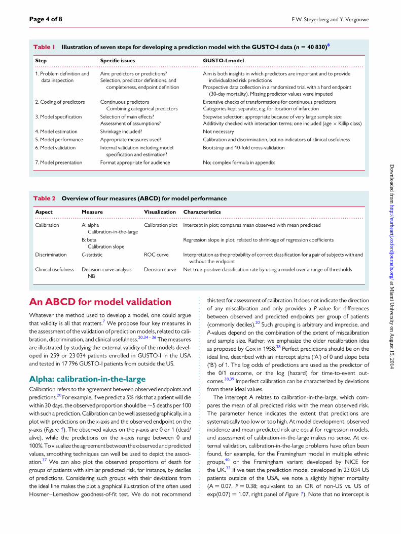
Table 1 Illustration of seven steps for developing a prediction model with the GUSTO-I data (n 5 40 830)8

Step Specific issues GUSTO-I model

1. Problem definition anddata inspection

Aim: predictors or predictions?Selection, predictor definitions, and

completeness, endpoint definition

Aim is both insights in which predictors are important and to provideindividualized risk predictions

Prospective data collection in a randomized trial with a hard endpoint(30-day mortality). Missing predictor values were imputed

2. Coding of predictors Continuous predictorsCombining categorical predictors

Extensive checks of transformations for continuous predictorsCategories kept separate, e.g. for location of infarction

3. Model specification Selection of main effects?Assessment of assumptions?

Stepwise selection; appropriate because of very large sample sizeAdditivity checked with interaction terms; one included (age × Killip class)

4. Model estimation Shrinkage included? Not necessary

5. Model performance Appropriate measures used? Calibration and discrimination, but no indicators of clinical usefulness

6. Model validation Internal validation including modelspecification and estimation?

Bootstrap and 10-fold cross-validation

7. Model presentation Format appropriate for audience No; complex formula in appendix

. . . . . . . . . . . . . . . . . . . . . . . . . . . . . . . . . . . . . . . . . . . . . . . . . . . . . . . . . . . . . . . . . . . . . . . . . . . . . . . . . . . . . . . . . . . . . . . . . . . . . . . . . . . . . . . . . . . . . . . . . . . . . . . . . . . . . . . . . . . . . . . . . . . . . . . . . . . . . . . . . . . . . . . . . . . . . . .

Table 2 Overview of four measures (ABCD) for model performance

Aspect Measure Visualization Characteristics

Calibration A: alphaCalibration-in-the-large

Calibration plot Intercept in plot; compares mean observed with mean predicted

B: betaCalibration slope

Regression slope in plot; related to shrinkage of regression coefficients

Discrimination C-statistic ROC curve Interpretation as the probability of correct classification for a pair of subjects with andwithout the endpoint

Clinical usefulness Decision-curve analysisNB

Decision curve Net true-positive classification rate by using a model over a range of thresholds

E.W. Steyerberg and Y. VergouwePage 4 of 8

at Miam

i University on A

ugust 15, 2014http://eurheartj.oxfordjournals.org/

Dow

nloaded from

calculated if a Cox model is used at external validation.36 We cancompare the mean of the predicted risks for a certain time point,e.g. 5 or 10 years, with the estimate from a Kaplan–Meier curve.Other types of models, such as Weibull regression models, canalso be used to assess calibration-in-the-large for survival models.41

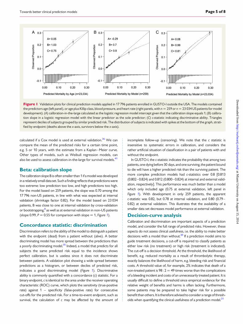
Beta: calibration slopeThe calibration slope B is often smaller than 1 if a model wasdevelopedin a relativelysmall data set. Suchafindingreflects thatpredictionsweretoo extreme: low prediction too low, and high predictions too high.For the model based on 259 patients, the slope was 0.70 among the17 796 non-US patients, in line with what was expected at internalvalidation (shrinkage factor 0.82). For the model based on 23 034patients, B was close to one at internal validation by cross-validationor bootstrapping,8 as well as at external validation in non-US patients(slope 0.99, P ¼ 0.55 for comparison with slope ¼ 1, Figure 1).

Concordance statistic: discriminationDiscrimination refers to the ability of the model to distinguish a patientwith the endpoint (dead) from a patient without (alive). A betterdiscriminating model has more spread between the predictions thana poorly discriminating model.35 Indeed, a model that predicts for allsubjects the same predicted risk equal to the incidence showsperfect calibration, but is useless since it does not discriminatebetween patients. A validation plot showing a wide spread betweenpredictions as a histogram, or between deciles of predicted risk,indicates a good discriminating model (Figure 1). Discriminativeability is commonly quantified with a concordance (c) statistic. For abinary endpoint, c is identical to the area under the receiver operatingcharacteristic (ROC) curve, which plots the sensitivity (true-positiverate) against 1 – specificity (false-positive rate) for consecutivecut-offs for the predicted risk. For a time-to-event endpoint, such assurvival, the calculation of c may be affected by the amount of

incomplete follow-up (censoring). We note that the c statistic isinsensitive to systematic errors in calibration, and considers therather artificial situation of classification in a pair of patients with andwithout the endpoint.

In GUSTO-I, the c-statistic indicates the probability that among twopatients, one dying before 30 days, and one surviving, the patient boundto die will have a higher predicted risk than the surviving patient. Themore complex prediction models had c-statistics over 0.8 [0.813(0.802–0.824) and 0.812 (0.800–0.824) at internal and external valid-ation, respectively]. This performance was much better than a modelwhich only included age (0.75 at external validation, left panel inFigure 1). With development in only 259 patients, the apparentc-statistic was 0.82, but 0.78 at internal validation, and 0.80 (0.79–0.82) at external validation. This illustrates that the availability of asmaller data set decreases model performance at external validation.

Decision-curve analysisCalibration and discrimination are important aspects of a predictionmodel, and consider the full range of predicted risks. However, theseaspects do not assess clinical usefulness, i.e. the ability to make betterdecisions with a model than without.20 If a prediction model aims toguide treatment decisions, a cut-off is required to classify patients aseither low risk (no treatment) or high risk (treatment is indicated).The cut-off is a decision threshold. At the threshold, the likelihood ofbenefit, e.g. reduced mortality as a result of thrombolytic therapy,exactly balances the likelihood of harm, e.g. bleeding risk and financialcosts. A threshold value of, for example, 2% indicates that death of anon-treated patient is 98 : 2¼ 49 times worse than the complicationsof a bleeding incident and costs of an unnecessarily treated patient. It isusually difficult to define a threshold since empirical evidence for therelative weight of benefits and harms is often lacking. Furthermore,some patients may be prepared to take higher risk for a possiblebenefit than others. It is therefore advised toconsidera rangeof thresh-olds when quantifying the clinical usefulness of a prediction model.21

Figure 1 Validation plots for clinical prediction models applied in 17 796 patients enrolled in GUSTO-I outside the USA. The models containedthe predictors age (left panel), or age plus Killip class, blood pressure, and heart rate (right panels, with n ¼ 259 or n ¼ 23 034 US patients for modeldevelopment). (A) calibration-in-the-large calculated as the logistic regression model intercept given that the calibration slope equals 1; (B) calibra-tion slope in a logistic regression model with the linear predictor as the sole predictor; (C) c-statistic indicating discriminative ability. Trianglesrepresent deciles of subjects grouped by similar predicted risk. The distribution of subjects is indicated with spikes at the bottom of the graph, strati-fied by endpoint (deaths above the x-axis, survivors below the x-axis).

Towards better clinical prediction models Page 5 of 8

at Miam

i University on A

ugust 15, 2014http://eurheartj.oxfordjournals.org/

Dow

nloaded from

Oncea thresholdhasbeenapplied toclassify patients as lowvs. highrisk, sensitivity and specificity are often used as measures for useful-ness. Finding an optimal balance between these is again possiblewithconsiderationofharmsandbenefitsof treatment, in combinationwith the incidence of the endpoint. The sum of sensitivity and speci-ficity can only be used as a naive summary indicator of usefulness,since such a sum ignores the relative weight of true positives (consid-ered in sensitivity) and false positives (considered in 1 – specificity).42

Recently proposed and more appropriate summary measuresinclude the net benefit (NB).21 This measure is consistent with theuseof anoptimal decision threshold toclassify patients.43 The relativeweight of harms and benefits is used to define the threshold, and isused to calculate a weighted sum of true- minus false-positiveclassifications.21

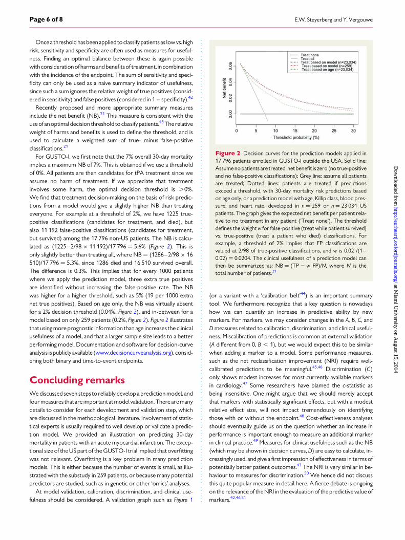
For GUSTO-I, we first note that the 7% overall 30-day mortalityimplies a maximum NB of 7%. This is obtained if we use a thresholdof 0%. All patients are then candidates for tPA treatment since weassume no harm of treatment. If we appreciate that treatmentinvolves some harm, the optimal decision threshold is .0%.We find that treatment decision-making on the basis of risk predic-tions from a model would give a slightly higher NB than treatingeveryone. For example at a threshold of 2%, we have 1225 true-positive classifications (candidates for treatment, and died), butalso 11 192 false-positive classifications (candidates for treatment,but survived) among the 17 796 non-US patients. The NB is calcu-lated as (1225–2/98 × 11 192)/17 796 ¼ 5.6% (Figure 2). This isonly slightly better than treating all, where NB ¼ (1286–2/98 × 16510)/17 796 ¼ 5.3%, since 1286 died and 16 510 survived overall.The difference is 0.3%. This implies that for every 1000 patientswhere we apply the prediction model, three extra true positivesare identified without increasing the false-positive rate. The NBwas higher for a higher threshold, such as 5% (19 per 1000 extranet true positives). Based on age only, the NB was virtually absentfor a 2% decision threshold (0.04%, Figure 2), and in-between for amodel based on only 259 patients (0.2%, Figure 2). Figure 2 illustratesthat using more prognostic information than age increases the clinicalusefulness of a model, and that a larger sample size leads to a betterperforming model. Documentation and software for decision-curveanalysis is publicly available (www.decisioncurveanalysis.org), consid-ering both binary and time-to-event endpoints.

Concluding remarksWe discussed seven steps to reliably develop a prediction model, andfour measures that are important atmodel validation. Therearemanydetails to consider for each development and validation step, whichare discussed in the methodological literature. Involvement of statis-tical experts is usually required to well develop or validate a predic-tion model. We provided an illustration on predicting 30-daymortality in patients with an acute myocardial infarction. The excep-tional size of the US part of the GUSTO-I trial implied that overfittingwas not relevant. Overfitting is a key problem in many predictionmodels. This is either because the number of events is small, as illu-strated with the substudy in 259 patients, or because many potentialpredictors are studied, such as in genetic or other ‘omics’ analyses.

At model validation, calibration, discrimination, and clinical use-fulness should be considered. A validation graph such as Figure 1

(or a variant with a ‘calibration belt’44) is an important summarytool. We furthermore recognize that a key question is nowadayshow we can quantify an increase in predictive ability by newmarkers. For markers, we may consider changes in the A, B, C, andD measures related to calibration, discrimination, and clinical useful-ness. Miscalibration of predictions is common at external validation(A different from 0, B , 1), but we would expect this to be similarwhen adding a marker to a model. Some performance measures,such as the net reclassification improvement (NRI) require well-calibrated predictions to be meaningful.45,46 Discrimination (C)only shows modest increases for most currently available markersin cardiology.47 Some researchers have blamed the c-statistic asbeing insensitive. One might argue that we should merely acceptthat markers with statistically significant effects, but with a modestrelative effect size, will not impact tremendously on identifyingthose with or without the endpoint.48 Cost-effectiveness analysesshould eventually guide us on the question whether an increase inperformance is important enough to measure an additional markerin clinical practice.49 Measures for clinical usefulness such as the NB(which may be shown in decision curves, D) are easy to calculate, in-creasingly used, and give a first impression of effectiveness in terms ofpotentially better patient outcomes.43 The NRI is very similar in be-haviour to measures for discrimination.50 We hence did not discussthis quite popular measure in detail here. A fierce debate is ongoingon the relevance of the NRI in the evaluation of the predictive value ofmarkers.42,46,51

Figure 2 Decision curves for the prediction models applied in17 796 patients enrolled in GUSTO-I outside the USA. Solid line:Assume no patients are treated, net benefit is zero (no true-positiveand no false-positive classifications); Grey line: assume all patientsare treated; Dotted lines: patients are treated if predictionsexceed a threshold, with 30-day mortality risk predictions basedon age only, or a prediction model with age, Killip class, blood pres-sure, and heart rate, developed in n ¼ 259 or n ¼ 23 034 USpatients. The graph gives the expected net benefit per patient rela-tive to no treatment in any patient (‘Treat none’). The thresholddefines the weight w for false-positive (treat while patient survived)vs. true-positive (treat a patient who died) classifications. Forexample, a threshold of 2% implies that FP classifications arevalued at 2/98 of true-positive classifications, and w is 0.02 /(1–0.02) ¼ 0.0204. The clinical usefulness of a prediction model canthen be summarized as: NB ¼ (TP 2 w FP)/N, where N is thetotal number of patients.21

E.W. Steyerberg and Y. VergouwePage 6 of 8

at Miam

i University on A

ugust 15, 2014http://eurheartj.oxfordjournals.org/

Dow

nloaded from

We see a role for our proposed framework to support methodo-logical researchers who develop and validate prediction models. Moreimportantly, clinical researchers may use the framework to systematical-ly and critically assess a publication where a prediction model is devel-oped or validated. We anticipate that following the framework,admittedly with room for refinements, will strengthen the methodo-logical rigourandqualityofpredictionmodels incardiovascular research.

FundingE.W.S. was supported by a U award (1U01-NS086294-01, value of perso-nalized risk information). Y.V. was supported by a VIDI grant (91711383,prognostic research with clustered data).

Conflict of interest: none declared.

Appendix

. . . . . . . . . . . . . . . . . . . . . . . . . . . . . . . . . . . . . . . . . . . . . . . . . . . . . . . . . . . . . . . . . . . . . . . . . . . . . . . . . . . . . . . . . . . . . . . . . . . . . . . . . . . . . . . . . . . . . . . . . . . . . . . . . . . . . . . . . . . . . . . . . . . . . . . . . . . . . . . . . . . . . . . . . . . . . . .

. . . . . . . . . . . . . . . . . . . . . . . . . . . . . . . . . . . . . . . . . . . . . . . . . . . . . . . . . . . . . . . . . . . . . . . . . . . . . . . . . . . . . . . . . . . . . . . . . . . . . . . . . . . . . . . . . . . . . . . . . . . . . . . . . . . . . . . . . . . . . . . . . . . . . . . . . . . . . . . . . . . . . . . . . . . . . . .

. . . . . . . . . . . . . . . . . . . . . . . . . . . . . . . . . . . . . . . . . . . . . . . . . . . . . . . . . . . . . . . . . . . . . . . . . . . . . . . . . . . . . . . . . . . . . . . . . . . . . . . . . . . . . . . . . . . . . . . . . . . . . . . . . . . . . . . . . . . . . . . . . . . . . . . . . . . . . . . . . . . . . . . . . . . . . . .

. . . . . . . . . . . . . . . . . . . . . . . . . . . . . . . . . . . . . . . . . . . . . . . . . . . . . . . . . . . . . . . . . . . . . . . . . . . . . . . . . . . . . . . . . . . . . . . . . . . . . . . . . . . . . . . . . . . . . . . . . . . . . . . . . . . . . . . . . . . . . . . . . . . . . . . . . . . . . . . . . . . . . . . . . . . . . . .

. . . . . . . . . . . . . . . . . . . . . . . . . . . . . . . . . . . . . . . . . . . . . . . . . . . . . . . . . . . . . . . . . . . . . . . . . . . . . . . . . . . . . . . . . . . . . . . . . . . . . . . . . . . . . . . . . . . . . . . . . . . . . . . . . . . . . . . . . . . . . . . . . . . . . . . . . . . . . . . . . . . . . . . . . . . . . . .

. . . . . . . . . . . . . . . . . . . . . . . . . . . . . . . . . . . . . . . . . . . . . . . . . . . . . . . . . . . . . . . . . . . . . . . . . . . . . . . . . . . . . . . . . . . . . . . . . . . . . . . . . . . . . . . . . . . . . . . . . . . . . . . . . . . . . . . . . . . . . . . . . . . . . . . . . . . . . . . . . . . . . . . . . . . . . . .

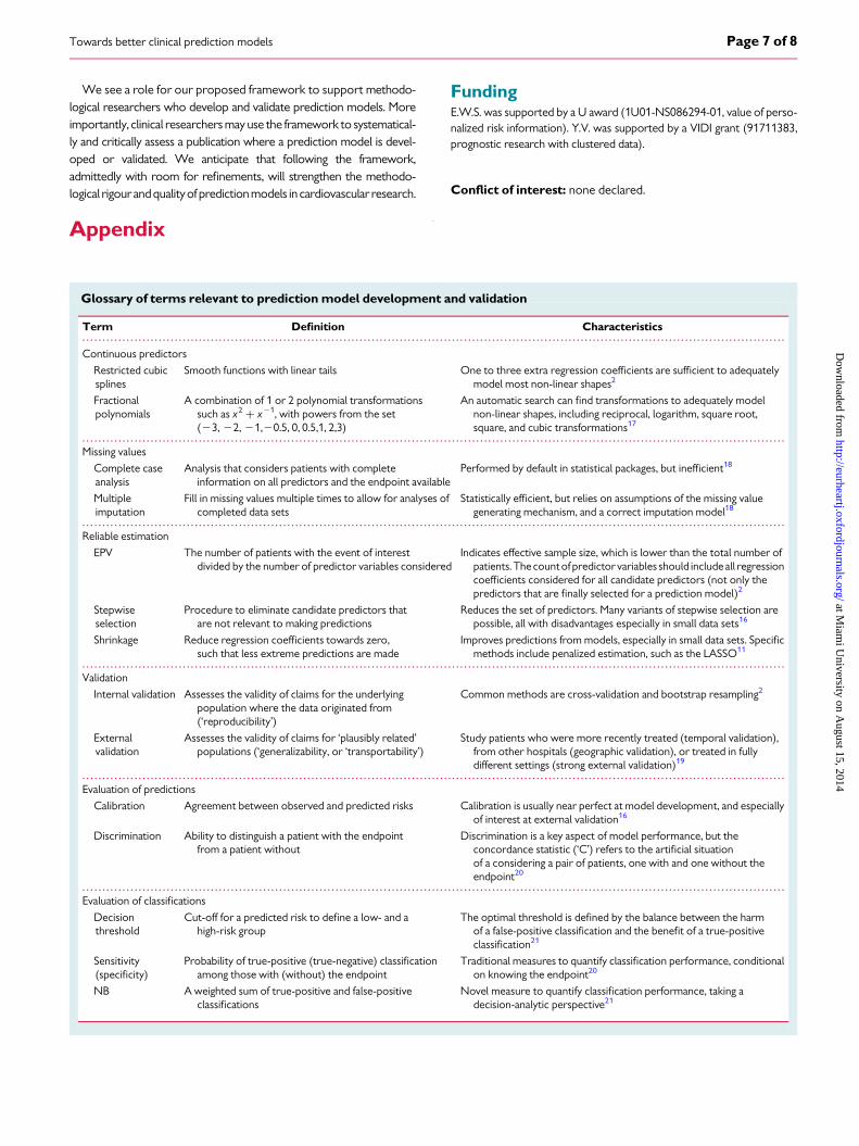
Glossary of terms relevant to prediction model development and validation

Term Definition Characteristics

Continuous predictors

Restricted cubicsplines

Smooth functions with linear tails One to three extra regression coefficients are sufficient to adequatelymodel most non-linear shapes2

Fractionalpolynomials

A combination of 1 or 2 polynomial transformationssuch as x2 + x21, with powers from the set(23, 22, 21,20.5, 0, 0.5,1, 2,3)

An automatic search can find transformations to adequately modelnon-linear shapes, including reciprocal, logarithm, square root,square, and cubic transformations17

Missing values

Complete caseanalysis

Analysis that considers patients with completeinformation on all predictors and the endpoint available

Performed by default in statistical packages, but inefficient18

Multipleimputation

Fill in missing values multiple times to allow for analyses ofcompleted data sets

Statistically efficient, but relies on assumptions of the missing valuegenerating mechanism, and a correct imputation model18

Reliable estimation

EPV The number of patients with the event of interestdivided by the number of predictor variables considered

Indicates effective sample size, which is lower than the total number ofpatients. The countof predictor variables should includeall regressioncoefficients considered for all candidate predictors (not only thepredictors that are finally selected for a prediction model)2

Stepwiseselection

Procedure to eliminate candidate predictors thatare not relevant to making predictions

Reduces the set of predictors. Many variants of stepwise selection arepossible, all with disadvantages especially in small data sets16

Shrinkage Reduce regression coefficients towards zero,such that less extreme predictions are made

Improves predictions from models, especially in small data sets. Specificmethods include penalized estimation, such as the LASSO11

Validation

Internal validation Assesses the validity of claims for the underlyingpopulation where the data originated from(‘reproducibility’)

Common methods are cross-validation and bootstrap resampling2

Externalvalidation

Assesses the validity of claims for ‘plausibly related’populations (‘generalizability, or ‘transportability’)

Study patients who were more recently treated (temporal validation),from other hospitals (geographic validation), or treated in fullydifferent settings (strong external validation)19

Evaluation of predictions

Calibration Agreement between observed and predicted risks Calibration is usually near perfect at model development, and especiallyof interest at external validation16

Discrimination Ability to distinguish a patient with the endpointfrom a patient without

Discrimination is a key aspect of model performance, but theconcordance statistic (‘C’) refers to the artificial situationof a considering a pair of patients, one with and one without theendpoint20

Evaluation of classifications

Decisionthreshold

Cut-off for a predicted risk to define a low- and ahigh-risk group

The optimal threshold is defined by the balance between the harmof a false-positive classification and the benefit of a true-positiveclassification21

Sensitivity(specificity)

Probability of true-positive (true-negative) classificationamong those with (without) the endpoint

Traditional measures to quantify classification performance, conditionalon knowing the endpoint20

NB A weighted sum of true-positive and false-positiveclassifications

Novel measure to quantify classification performance, taking adecision-analytic perspective21

Towards better clinical prediction models Page 7 of 8

at Miam

i University on A

ugust 15, 2014http://eurheartj.oxfordjournals.org/

Dow

nloaded from

References1. Van de Werf F, Bax J, Betriu A, Blomstrom-Lundqvist C, Crea F, Falk V, Filippatos G,

Fox K, Huber K, Kastrati A, Rosengren A, Steg PG, Tubaro M, Verheugt F,Weidinger F, Weis M. Guidelines ESCCfP. Management of acute myocardial infarc-tion in patients presenting with persistent ST-segment elevation: the Task Force onthe Management of ST-Segment Elevation Acute Myocardial Infarction of the Euro-pean Society of Cardiology. Eur Heart J 2008;29:2909–2945.

2. Harrell FE. Regression Modeling Strategies: With Applications to Linear Models, LogisticRegression, and Survival Analysis. New York: Springer, 2001.

3. Moons KG, Royston P, Vergouwe Y, Grobbee DE, Altman DG. Prognosis and prog-nostic research: what, why, and how? BMJ 2009;338:b375.

4. Mushkudiani NA, Hukkelhoven CW, Hernandez AV, Murray GD, Choi SC, Maas AI,Steyerberg EW. A systematic review finds methodological improvements necessaryfor prognostic models in determining traumatic brain injury outcomes. J Clin Epide-miol 2008;61:331–343.

5. Mallett S, Royston P, Dutton S, Waters R, Altman DG. Reporting methods in studiesdeveloping prognostic models in cancer: a review. BMC Med 2010;8:20.

6. Bouwmeester W, Zuithoff NP, Mallett S, Geerlings MI, Vergouwe Y, Steyerberg EW,Altman DG, Moons KG. Reporting and methods in clinical prediction research: a sys-tematic review. PLoS Med 2012;9:1–12.

7. Collins GS, de Groot JA, Dutton S, Omar O, Shanyinde M, Tajar A, Voysey M,Wharton R, Yu LM, Moons KG, Altman DG. External validation of multivariable pre-diction models: a systematic review of methodological conduct and reporting. BMCMed Res Methodol 2014;14:40.

8. Lee KL, Woodlief LH, Topol EJ, Weaver WD, Betriu A, Col J, Simoons M, Aylward P,Van de Werf F, Califf RM. Predictors of 30-day mortality in the era of reperfusion foracute myocardial infarction. Results from an international trial of 41,021 patients.GUSTO-I Investigators. Circulation 1995;91:1659–1668.

9. Ennis M, Hinton G, Naylor D, Revow M, Tibshirani R. A comparison of statisticallearning methods on the GUSTO database. Stat Med 1998;17:2501–2508.

10. Steyerberg EW, Eijkemans MJ, Habbema JD. Stepwise selection in small data sets: asimulation study of bias in logistic regression analysis. J Clin Epidemiol 1999;52:935–942.

11. Steyerberg EW, Eijkemans MJ, Harrell FE Jr, Habbema JD. Prognostic modelling withlogistic regression analysis: a comparison of selection and estimation methods insmall data sets. Stat Med 2000;19:1059–1079.

12. Steyerberg EW, Eijkemans MJ, Harrell FE Jr, Habbema JD. Prognostic modeling withlogistic regression analysis: in searchof a sensible strategy in small data sets. Med DecisMaking 2001;21:45–56.

13. Steyerberg EW, Harrell FE Jr, Borsboom GJ, Eijkemans MJ, Vergouwe Y,Habbema JD. Internal validation of predictive models: efficiency of some proceduresfor logistic regression analysis. J Clin Epidemiol 2001;54:774–781.

14. Steyerberg EW, Borsboom GJ, van Houwelingen HC, Eijkemans MJ, Habbema JD.Validation and updating of predictive logistic regression models: a study on samplesize and shrinkage. Stat Med 2004;23:2567–2586.

15. Steyerberg EW, Eijkemans MJ, Boersma E, Habbema JD. Equally valid models gavedivergent predictions for mortality in acute myocardial infarction patients in a com-parison of logistic regression models. J Clin Epidemiol 2005;58:383–390.

16. Steyerberg EW. Clinical Prediction Models: A Practical Approach to Development,Validation, and Updating. New York: Springer, 2009.

17. Royston P, Sauerbrei W. Multivariable Model-building: A Pragmatic Approach to Regres-sion Analysis Based on Fractional Polynomials for Modelling Continuous Variables. Chich-ester, England, Hoboken, NJ: John Wiley, 2008.

18. Altman DG, Bland JM. Missing data. BMJ 2007;334:424.19. Justice AC, Covinsky KE, Berlin JA. Assessing the generalizability of prognostic infor-

mation. Ann Intern Med 1999;130:515–524.20. Steyerberg EW, Vickers AJ, Cook NR, Gerds T, Gonen M, Obuchowski N,

Pencina MJ, Kattan MW. Assessing the performance of prediction models: a frame-work for traditional and novel measures. Epidemiology 2010;21:128–138.

21. VickersAJ, ElkinEB. Decision curveanalysis: a novelmethod forevaluatingpredictionmodels. Med Decis Making 2006;26:565–574.

22. Shmueli G. To explain or to predict? Statist Sci 2010;25:289–310.23. Kattan MW. Doc, what are my chances? A conversation about prognostic uncer-

tainty. Eur Urol 2011;59:224.24. Hauck WW, Anderson S, Marcus SM. Should we adjust for covariates in nonlinear

regression analyses of randomized trials? Control Clin Trials 1998;19:249–256.25. Steyerberg EW, Bossuyt PM, Lee KL. Clinical trials in acute myocardial infarction:

should we adjust for baseline characteristics? Am Heart J 2000;139:745–751.26. Genders TS, Steyerberg EW, Alkadhi H, Leschka S, Desbiolles L, Nieman K,

Galema TW, Meijboom WB, Mollet NR, de Feyter PJ, Cademartiri F, Maffei E,

Dewey M, Zimmermann E, Laule M, Pugliese F, Barbagallo R, Sinitsyn V, Bogaert J,Goetschalckx K, Schoepf UJ, Rowe GW, Schuijf JD, Bax JJ, de Graaf FR, Knuuti J,Kajander S, van Mieghem CA, Meijs MF, Cramer MJ, Gopalan D, Feuchtner G,Friedrich G, Krestin GP, Hunink MG, Consortium CAD. A clinical prediction rulefor the diagnosis of coronary artery disease: validation, updating, and extension.Eur Heart J 2011;32:1316–1330.

27. Royston P, Altman DG, Sauerbrei W. Dichotomizing continuous predictors inmultiple regression: a bad idea. Stat Med 2006;25:127–141.

28. Boersma E, Poldermans D, Bax JJ, Steyerberg EW, Thomson IR, Banga JD, van DeVen LL, van Urk H, Roelandt JR, Group DS. Predictors of cardiac events aftermajor vascular surgery: role of clinical characteristics, dobutamine echocardiog-raphy, and beta-blocker therapy. JAMA 2001;285:1865–1873.

29. Derksen S, Keselman H. Backward, forward and stepwise automated subset selec-tion algorithms: frequency of obtaining authentic and noise variables. Br J Math StatPsychol 1992;45:265–282.

30. van Houwelingen JC, Le Cessie S. Predictive value of statistical models. Stat Med1990;9:1303–1325.

31. Moons KG, Donders AR, Steyerberg EW, Harrell FE. Penalized maximum likelihoodestimation to directly adjust diagnostic and prognostic prediction models for over-optimism: a clinical example. J Clin Epidemiol 2004;57:1262–1270.

32. Tibshirani R. Regression and shrinkage via the Lasso. J R Stat Soc Ser B 1996;58:267–288.

33. Collins GS, Altman DG. Predicting the 10 year risk of cardiovascular disease in theUnited Kingdom: independent and external validation of an updated version ofQRISK2. BMJ 2012;344:e4181.

34. Vergouwe Y, Steyerberg EW, Eijkemans MJ, Habbema JD. Validity of prognosticmodels: when is a model clinically useful? Semin Urol Oncol 2002;20:96–107.

35. Royston P, Altman DG. Visualizing and assessing discrimination in the logistic regres-sion model. Stat Med 2010;29:2508–2520.

36. RoystonP, Altman DG. External validation of aCoxprognosticmodel: principles andmethods. BMC Med Res Methodol 2013;13:33.

37. Austin PC, Steyerberg EW. Graphical assessment of internal and external calibrationof logistic regression models by using loess smoothers. Stat Med 2014;33:517–535.

38. Cox DR. Two further applications of a model for binary regression. Biometrika 1958;45:562–565.

39. Miller ME, Langefeld CD, Tierney WM, Hui SL, McDonald CJ. Validation of probabil-istic predictions. Med Decis Making 1993;13:49–58.

40. D’Agostino RB Sr, Grundy S, Sullivan LM, Wilson P. Validation of the Framinghamcoronary heart disease prediction scores: results of a multiple ethnic groups inves-tigation. JAMA 2001;286:180–187.

41. van Houwelingen HC, Thorogood J. Construction, validation and updating of a prog-nostic model for kidney graft survival. Stat Med 1995;14:1999–2008.

42. Greenland S. The need for reorientation toward cost-effective prediction. Stat Med2008;27:199–206.

43. Localio AR, Goodman S. Beyond the usual prediction accuracy metrics: reportingresults for clinical decision making. Ann Intern Med 2012;157:294–295.

44. Nattino G, Finazzi S, Bertolini G. A new calibration test and a reappraisal of the cali-bration belt for the assessment of prediction models based on dichotomous out-comes. Stat Med 2014; in press. PMID 24497413.

45. Pencina MJ, D’Agostino RB Sr, Steyerberg EW. Extensions of net reclassification im-provement calculations to measureusefulnessof newbiomarkers. StatMed 2011;30:11–21.

46. Leening MJ, Vedder MM, Witteman JC, Pencina MJ, Steyerberg EW. Net reclassifica-tion improvement: computation, interpretation, and controversies: a literaturereview and clinician’s guide. Ann Intern Med 2014;160:122–131.

47. Tzoulaki I, Liberopoulos G, Ioannidis JP. Assessment of claims of improved predic-tion beyond the Framingham risk score. Jama 2009;302:2345–2352.

48. Pepe MS, Janes H, Longton G, Leisenring W, Newcomb P. Limitations of the oddsratio in gauging the performance of a diagnostic, prognostic, or screening marker.Am J Epidemiol 2004;159:882–890.

49. Hlatky MA, Greenland P, Arnett DK, Ballantyne CM, Criqui MH, Elkind MS, Go AS,Harrell FE Jr, Hong Y, Howard BV, Howard VJ, Hsue PY, Kramer CM, McConnell JP,Normand SL, O’Donnell CJ, Smith SC Jr, Wilson PW. Criteria for evaluation of novelmarkers of cardiovascular risk: a scientific statement from the American Heart As-sociation. Circulation 2009;119:2408–2416.

50. Van Calster B, Vickers AJ, Pencina MJ, Baker SG, Timmerman D, Steyerberg EW.Evaluation of markers and risk prediction models: overview of relationshipsbetween NRI and decision-analytic measures. Med Decis Making 2013;33:490–501.

51. Vickers AJ, Pepe M. Does the net reclassification improvement help us evaluatemodels and markers?. Ann Intern Med 2014;160:136–137.

E.W. Steyerberg and Y. VergouwePage 8 of 8

at Miam

i University on A

ugust 15, 2014http://eurheartj.oxfordjournals.org/

Dow

nloaded from