total generalised variation in di usion tensor imaging · total generalised variation in di usion...
TRANSCRIPT

Total generalised variation in diffusion tensor imaging
Tuomo Valkonen∗, Kristian Bredies†, and Florian Knoll‡
Abstract. We study the extension of total variation (TV), total deformation (TD), and (second-order) totalgeneralised variation (TGV2) to symmetric tensor fields. We show that for a suitable choice offinite-dimensional norm, these variational semi-norms are rotation-invariant in a sense natural andwell-suited for application to diffusion tensor imaging (DTI). Combined with a positive definitenessconstraint, we employ these novel semi-norms as regularisers in ROF-type denoising of medicalin-vivo brain images. For the numerical realisation, we employ the Chambolle-Pock algorithm,for which we develop a novel duality-based stopping criterion which guarantees error bounds withrespect to the functional values. Our findings indicate that TD and TGV2, both of which employthe symmetrised differential, provide improved results compared to other evaluated approaches.
Key words. total variation, total deformation, total generalised variation, regularisation, medical imaging,diffusion tensor imaging.
AMS subject classifications. 92C55, 94A08, 26B30, 49M29
1. Introduction. In this paper, we propose and study novel edge-preserving regularisa-tion functionals for positivity-constrained variational denoising problems on symmetric tensorfields, i.e., minimising functionals of the type
minu≥0
1
2‖f − u‖2F,2 +H(u). (1.1)
Here, f ∈ L1(Ω; Sym2(Rm)) is a second-order symmetric tensor field on a domain Ω ⊂ Rm,‖ · ‖F,2 is the L2-norm on Ω with Frobenius norm for symmetric 2-tensors as pointwise norm,and H is a regularisation functional. Observe, moreover, that we require the solution u ∈L1(Ω; Sym2(Rm)) to be pointwise a.e. positive semi-definite. The regularisation functionalswe are introducing in this paper generalise the total-variation functional
H(u) = ‖Du‖M(Ω;),
extended to symmetric tensor fields of order k, which is a popular choice for denoising problemsand usually results in the ROF (Rudin-Osher-Fatemi [34]) model. The generalisations areaiming at two directions. On the one hand, we utilise the symmetrised derivative Eu of uinstead of the full derivative Du in order to obtain a weaker measure of gradient information.This results in the total deformation, which reads as
H(u) = ‖Eu‖M(Ω;Symk+1(Rm))
and can also be seen as first-order total generalised variation TGV1 for tensor fields. In par-ticular, it imposes, as the total variation, regularity on the data which includes discontinuities
∗Institute for Mathematics and Scientific Computing, University of Graz, Austria. [email protected].†Institute for Mathematics and Scientific Computing, University of Graz, Austria. [email protected]‡Institute of Medical Engineering, Graz University of Technology, Austria. [email protected]
1

2 T. Valkonen, K. Bredies, and F. Knoll
and is therefore well-suited for symmetric tensor-valued image data. However, like all Radon-type first-order regularisations, solutions tend to exhibit staircasing artefacts. In order toreduce these effects we also propose, on the other hand, a generalisation of the second-ordertotal generalised variation TGV2 [11] for symmetric tensor fields:
H(u) = minw∈L1(Ω;Symk+1(Rm))
α‖Eu− w‖M(Ω;Symk+1(Rm)) + β‖Ew‖M(Ω;Symk+2(Rm)).
Besides providing an analysis for these functionals and the associated denoising problems, wemoreover develop and discuss a numerical algorithm for the approximate solution of theseproblems together with a rigorous stopping criterion. The performance of the algorithm istested on synthetic as well as in-vivo brain data.
The need for solving positivity-constrained denoising problems with tensor-valued dataarises, for instance, in diffusion-tensor imaging (DTI) of brain tissues. As a first step towardsDTI, diffusion weighted magnetic resonance imaging (DWI) is performed. It measures theanisotropic diffusion of water molecules, and provides valuable and unique in-vivo insight intothe white matter structure of the brain [8, 38]. To capture the diffusion information, imageshave to be obtained with diffusion sensitising gradients in multiple directions. This leads tovery long acquisition times, even with ultra fast sequences like echo planar imaging (EPI).Therefore, DWI is inherently a low-resolution and low-SNR method. It exhibits Rician noise[23], eddy-current distortions [38], and is very sensitive with respect to artefacts originatingfrom patient motion [25, 2].
By taking multiple DWI images, a diffusion-tensor describing the probability of waterdiffusing in different spatial directions can be solved from the Stejskal-Tanner equation [8, 27].These tensors can be visualised as a confidence ellipsoids, which have varying anisotropy – ordirectional dependence – depending on the probability of diffusion of water in that direction.In particular, in the brain, grey matter has low anisotropy – the ellipsoids are almost spheres,water having uniform diffusion. In white matter, which transmits messages between areas ofgrey matter, the anisotropy is, by contrast, high – the ellipsoids are far from spheres, andwater has a single most probable direction of diffusion. Since the DWI measurements arenoisy, as described in the previous paragraph, we are led to the problem of denoising thediffusion tensors obtained this way. A natural requirement is that the denoising result shouldbe invariant with respect to rotations of the imaged object. In diffusion tensor imaging, unlikein scalar imaging, this involves individual tensors rotating as well, not only shifting to anotherpoint of the domain. Our regularisation functionals will be rotation-invariant. The denoisedtensors should, moreover, be positive definite, as the failure of this condition is non-physical.
Let us shortly discuss some of the existing approaches for the denoising of DTI dataand their relations to the present work. In [5, 6, 20, 21, 22] log-Euclidean metrics giving asuitable Riemannian manifold structure to Sym2(Rm) have been studied in the context ofdiffusion-tensor imaging. Regularisation approaches based on log-Euclidean metrics facilitatemaintaining the positive definiteness of the tensors, as well as avoiding swelling, i.e., increase involume of the ellipsoids corresponding to the tensors. Log-Euclidean metrics have, moreover,the advantage over earlier affine-invariant metrics [32] that they are computationally moreefficient. Basically the approach amounts to taking the logarithm of the data, to expand thepositive definite cone to the whole space, applying usual Euclidean techniques such as ROF

Total generalised variation in DTI 3
with smoothed TV regularisation term [20], or Gaussian denoising [21], and transformingthe solution back to the positive definite cone by taking the exponential. This approach hastherefore many desirable theoretical qualities, and is also computationally tractable. We areinterested in whether our regularisation approaches can provide results with other desirablequalities. It is known [11, 28] that TGV2 in the scalar case tends to avoid the stair-casingeffect exhibited by TV, so we expect some improvements. It is also interesting to see what isthe effect of the symmetrised differential employed by TD (that is to say, TGV1) and TGV2
in contrast to the normal differential employed by TV.
We note that TV, however lacking the positive semi-definiteness constraint, has in factalready been studied in [35]. In [24], which also takes the approach of Riemannian metrics, and[43], the positive semi-definiteness constraint is incorporated through a Cholesky or u = LDLT
factorisation approach. These two works moreover incorporate the Stejskal-Tanner equationinto the fidelity function, resulting in a difficult non-convex problem. The problem (1.1) is stillconvex, albeit constrained. Our novel algorithm, based on recent state-of-the-art non-smoothoptimisation methods [15], can however handle the constraint efficiently.
A completely different approach to DTI denoising is taken in [16, 40], similar to theone in [39] for colour images. It is of the Perona-Malik or anisotropic diffusion [44] type.Instead of directly minimising a regularisation functional, a constrained gradient flow of atime-dependent tensor field t 7→ ut is defined on a suitable manifold. The structure of thismanifold incorporates any desired constraints, such as positive semi-definiteness of ut(x), orthe magnitude of the eigenvalues of ut(x), if we only want to regularise the eigenvectors, asis also done in [33, 17]. The gradient flow is then used to transport the noisy measurementu0 = f until a solution ut of desired quality is found. Choosing the cost function giving riseto the (unconstrained) gradient flow to have suitable anisotropic smoothing properties, edgesshould be preserved – empirically, in the discretisation. Indeed, Perona-Malik type approachesin general have the theoretical difficulty that the edges in space appear in time as shocks thatcause the solution to break down. An obvious advantage of our approach (1.1) is that it alsotheoretically preserves edges (between white matter and grey matter), being based on rigorousformulations of L1 gradient penalties.
The rest of our paper is organised as follows. First in Section 2 we begin by introducingtensor and tensor field calculus to set up the framework in which our results are represented.We then define variational semi-norms of tensor fields, and show that these are rotation-invariant in a sense natural to diffusion tensor imaging. In Section 3 we introduce in moredetail the positivity-constrained denoising problems (1.1) with TV, TD, and TGV2 regulari-sation term, and show the existence of solutions. This involves a few new proofs, because wedefine TGV2 directly through the differentiation cascade formulation, which is more practicalfor numerical realisation than the original dual-ball formulation. After that, in Section 4,we describe our implementation of the Chambolle-Pock algorithm [15] that we use to solvethese problems, and represent a novel duality-based stopping criterion. Finally, in Section 5we study the numerical results that we have obtained, on both synthetic test data and anin-vivo brain measurement. To conclude the paper, we state in Section 6 our conclusionsand outlook for future research. Additionally, in Appendix A we show that the extra primalvariable of the differentiation cascade formulation of TGV2 is bounded, and in Appendix Bdiscuss alternative rotation-invariant tensor norms.

4 T. Valkonen, K. Bredies, and F. Knoll
2. Tensors and tensor fields. The development of total generalised variation demandsthe machinery of differential calculus of tensor fields that we derive next. We also show thatthe derived total variation and total deformation semi-norms of tensor fields are rotation-invariant, in a sense to be discussed in more detail, when the base finite-dimensional norm isthe Frobenius norm, or one of the alternatives discussed in Appendix B.
2.1. Basic tensor calculus. We begin by recalling basic tensor calculus. We make somesimplifications as we do not need the machinery in its full differential-geometric glory, as can befound in, e.g., [9]. In particular, as we are working on the Euclidean space Rm, and do not needtensors with simultaneous covariant (x ∈ Rm) and contravariant variables (x ∈ (Rm)∗ ∼ Rm),we make no distinction between them.
Therefore, we define a k-tensor A ∈ T k(Rm) as a k-linear mapping A : Rm×· · ·×Rm → R.A symmetric tensor A ∈ Symk(Rm) then satisfies for any permutation π of 1, . . . , k thatA(cπ1, . . . , cπk) = A(c1, . . . , ck).
For any A ∈ T k(Rm) we define the symmetrisation |||A by
(|||A)(c1, . . . , ck) :=1
k!
∑π
A(cπ1, . . . , cπk),
where the sum is taken over all k! permutations π of 1, . . . , k. For a k-tensor A and am-tensor B, we define the (m+ k)-tensor A⊗B by
(A⊗B)(c1, . . . , cm, cm+1, . . . , cm+k) = A(c1, . . . , cm)B(cm+1, . . . , cm+k).
Let then e1, . . . , em be the standard basis of Rm. We define the inner product
〈A,B〉 :=∑
p∈1,...,mkA(ep1 , . . . , epk)B(ep1 , . . . , epk), (2.1)
and the Frobenius norm‖A‖F :=
√〈A,A〉.
We will see later in Proposition 2.2 that these are invariant with respect to orthogonal basistransformations. We moreover have 〈A, |||B〉 = 〈|||A,B〉. Thus, in particular, for symmetricB ∈ Symk(Rm), and general A ∈ T k(Rm), we have 〈A,B〉 = 〈|||A,B〉.
Example 2.1 (Vectors). Vectors A ∈ Rm can be identified with symmetric 1-tensors: A(x) =〈A, x〉. The symmetrisation satisfies |||A = A. The inner product is the usual inner productin Rm, and the Frobenius norm ‖A‖F = ‖A‖2.
Example 2.2 (Matrices). Matrices can be identified with 2-tensors: A(x, y) = 〈Ax, y〉. Sym-metric matrices A = AT can be identified with symmetric 2-tensors. The symmetrisation isgiven by |||A = (A+AT )/2. The inner product is 〈A,B〉 =
∑i,j AijBij and ‖A‖F is the matrix
Frobenius norm. We use the notation A ≥ 0 for positive semi-definite A.Much of what follows in this section is stated for general tensor norms, although our numer-
ical work will employ the Frobenius norm. Appendix B however contains a discussion of somealternative norms, the so-called largest and smallest reasonable cross-norms. The applicationof these could provide interesting results, provided an efficient numerical implementation. Wetherefore do not fix the norm in the following when not necessary.

Total generalised variation in DTI 5
2.2. Tensor fields. Let ‖·‖• be a norm on T k(Rm). We denote its dual norm with respectto the inner product (2.1) by ‖ · ‖∗. For u : Ω→ T k(Rm) on a domain Ω ⊂ Rm, we then set
‖u‖•,p :=(∫
Ω‖u(x)‖p• dx
)1/p, (p ∈ [1,∞)), and ‖u‖•,∞ := ess supx∈Ω ‖u(x)‖•,
and define the spaces
Lp(Ω; T k(Rm)) = u : Ω→ T k(Rm) | ‖u‖•,p <∞, and
Lp(Ω; Symk(Rm)) = u : Ω→ Symk(Rm) | ‖u‖•,p <∞, (p ∈ [1,∞]).
The choice of the finite-dimensional norm ‖ · ‖• does not affect the definition of these spaces,since all finite-dimensional norms are equivalent. Hence strong and weak convergence in thespaces is unambiguously defined, with the dual spaces analogous to the case of scalar func-tions: for 1 ≤ p <∞, the dual of Lp(Ω; T k(Rm)) (resp. Lp(Ω; Symk(Rm))) is Lq(Ω; T k(Rm))(resp. Lq(Ω; Symk(Rm))), where q is the Holder conjugate of p, satisfying 1/p + 1/q = 1. Ina standard fashion we also deduce that ‖ · ‖•,p is lower semi-continuous with respect to weakconvergence in Lp.
A tensor field ϕ : Ω→ T k(Rm) is symmetrised pointwise, that is
(|||ϕ)(x) := |||(ϕ(x)).
We say that ϕ is symmetric, if ϕ(x) ∈ Symk(Rm) for every x ∈ Ω.We define for u ∈ C1(Ω; T k(Rm)), k ≥ 1 the divergence div u ∈ C(Ω; T k−1(Rm) by
contraction as
[div u(x)](ei2 , . . . , eik) :=
m∑i1=1
∂i1 [x 7→ u(x)(ei1 , . . . , eik)] =
m∑i1=1
〈ei1 ,∇u(·)(ei1 , . . . , eik)〉. (2.2)
Observe that if u is symmetric, then so is div u. This definition is also the reason why haveassumed the dimension m of the space Rm ⊃ Ω 3 x and of the parameters of u(x) ∈ T k(Rm)to agree. The definition of divergence does not as such apply to tensor fields u : RK → T k(Rm)for K 6= m. As our regularisation functionals will be based on calculating divergences (2.2),this has the implication that when we want to denoise 3D diffusion tensors, we should inprinciple have a full 3D volume Ω of data, not a 2D slice! We will return to this topic lateron.
Example 2.3 (Vector fields). Let u ∈ C1(Ω;Rm) = C1(Ω; T 1(Rm)). Then div u(x) =∑mi=1 ∂iui(x) is the usual divergence.
Example 2.4 (Matrix fields). Let u ∈ C1(Ω; T 2(Rm)). Then [div u(x)]j =∑m
i=1 ∂iuij(x).That is, we take columnwise the divergence of a vector field. We use the notation u ≥ 0 forpointwise a.e. positive semi-definite u.
Preparing to define tensor-valued measures next, we define the non-symmetric unit ball
V k∗,ns := ϕ ∈ C∞c (Ω; T k(Rm)) | ‖ϕ‖∗,∞ ≤ 1, (2.3)
and the symmetric unit ball
V k∗,s := ϕ ∈ C∞c (Ω; Symk(Rm)) | ‖ϕ‖∗,∞ ≤ 1.
6 T. Valkonen, K. Bredies, and F. Knoll
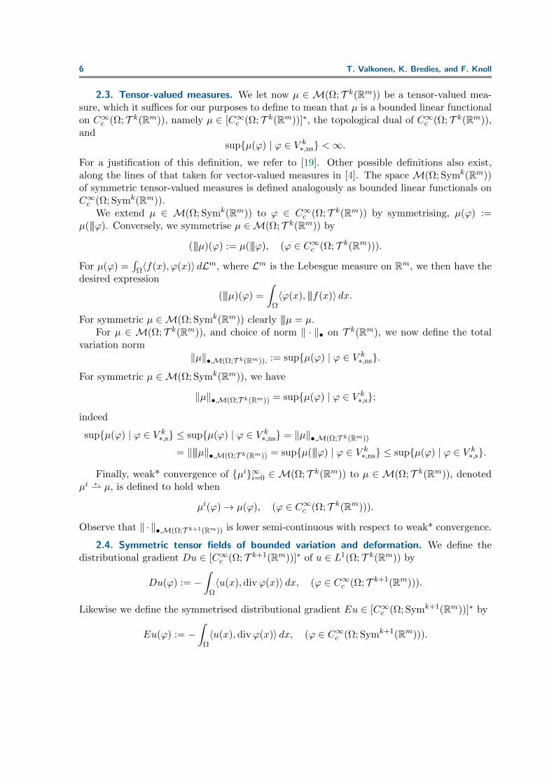
2.3. Tensor-valued measures. We let now µ ∈ M(Ω; T k(Rm)) be a tensor-valued mea-sure, which it suffices for our purposes to define to mean that µ is a bounded linear functionalon C∞c (Ω; T k(Rm)), namely µ ∈ [C∞c (Ω; T k(Rm))]∗, the topological dual of C∞c (Ω; T k(Rm)),and
supµ(ϕ) | ϕ ∈ V k∗,ns <∞.
For a justification of this definition, we refer to [19]. Other possible definitions also exist,along the lines of that taken for vector-valued measures in [4]. The space M(Ω; Symk(Rm))of symmetric tensor-valued measures is defined analogously as bounded linear functionals onC∞c (Ω; Symk(Rm)).
We extend µ ∈ M(Ω; Symk(Rm)) to ϕ ∈ C∞c (Ω; T k(Rm)) by symmetrising, µ(ϕ) :=µ(|||ϕ). Conversely, we symmetrise µ ∈M(Ω; T k(Rm)) by
(|||µ)(ϕ) := µ(|||ϕ), (ϕ ∈ C∞c (Ω; T k(Rm))).
For µ(ϕ) =∫
Ω〈f(x), ϕ(x)〉 dLm, where Lm is the Lebesgue measure on Rm, we then have thedesired expression
(|||µ)(ϕ) =
∫Ω〈ϕ(x), |||f(x)〉 dx.
For symmetric µ ∈M(Ω; Symk(Rm)) clearly |||µ = µ.For µ ∈ M(Ω; T k(Rm)), and choice of norm ‖ · ‖• on T k(Rm), we now define the total
variation norm‖µ‖•,M(Ω;T k(Rm)), := supµ(ϕ) | ϕ ∈ V k
∗,ns.
For symmetric µ ∈M(Ω; Symk(Rm)), we have
‖µ‖•,M(Ω;T k(Rm)) = supµ(ϕ) | ϕ ∈ V k∗,s;
indeed
supµ(ϕ) | ϕ ∈ V k∗,s ≤ supµ(ϕ) | ϕ ∈ V k
∗,ns = ‖µ‖•,M(Ω;T k(Rm))
= ‖|||µ‖•,M(Ω;T k(Rm)) = supµ(|||ϕ) | ϕ ∈ V k∗,ns ≤ supµ(ϕ) | ϕ ∈ V k
∗,s.
Finally, weak* convergence of µi∞i=0 ∈ M(Ω; T k(Rm)) to µ ∈ M(Ω; T k(Rm)), denotedµi ∗ µ, is defined to hold when
µi(ϕ)→ µ(ϕ), (ϕ ∈ C∞c (Ω; T k(Rm))).
Observe that ‖ · ‖•,M(Ω;T k+1(Rm)) is lower semi-continuous with respect to weak* convergence.
2.4. Symmetric tensor fields of bounded variation and deformation. We define thedistributional gradient Du ∈ [C∞c (Ω; T k+1(Rm))]∗ of u ∈ L1(Ω; T k(Rm)) by
Du(ϕ) := −∫
Ω〈u(x), divϕ(x)〉 dx, (ϕ ∈ C∞c (Ω; T k+1(Rm))).
Likewise we define the symmetrised distributional gradient Eu ∈ [C∞c (Ω; Symk+1(Rm))]∗ by
Eu(ϕ) := −∫
Ω〈u(x), divϕ(x)〉 dx, (ϕ ∈ C∞c (Ω; Symk+1(Rm))).

Total generalised variation in DTI 7
With these notions at hand, we now define the spaces of symmetric tensor fields of boundedvariation and bounded deformation, respectively, as (see also [10])
BV(Ω; Symk(Rm)) :=u ∈ L1(Ω; Symk(Rm))
∣∣∣ supϕ∈V k+1∗,ns
Du(ϕ) <∞, and
BD(Ω; Symk(Rm)) :=u ∈ L1(Ω; Symk(Rm))
∣∣∣ supϕ∈V k+1∗,s
Eu(ϕ) <∞.
For functions u ∈ BV(Ω; Symk(Rm)), we have Du ∈ M(Ω; T k+1(Rm)), that is, the operatorDu is a measure. Analogously, for u ∈ BD(Ω; Symk(Rm)), it holds Eu ∈M(Ω; Symk+1(Rm)).
Remark 2.1 (Equivalences and terminology). For k = 0, i.e., in the case of scalar fields, thespace BV(Ω; Sym0(Rm)) = BD(Ω; Sym0(Rm)) agrees with the usual space of (scalar) functionsof bounded variation. For k = 1, i.e., the case of vector fields, the space BD(Ω; Sym1(Rm))agrees with the space of functions of bounded deformation studied in [37]. This is our motiva-tion for the term tensor fields of bounded deformation. The space BD(Ω; Sym1(Rm)) does notagree with the space BV(Ω; Sym1(Rm)) for m > 1, as the kernel of E includes the infinites-imal rigid displacements u(x) = u0 + Ax, where A is skew-symmetric, while the kernel of Dincludes only constants.
Remark 2.2 (Symmetric tensor fields). It can be argued that from the point of view of gen-eral theory, the space
BV(Ω; T k(Rm)) :=u ∈ L1(Ω; T k(Rm))
∣∣∣ supϕ∈V k+1F,ns
Du(ϕ) <∞,
of general tensor fields of bounded variation is more natural than the space BV(Ω; Symk(Rm))of symmetric tensor fields of bounded variation. Indeed, in the former case neither u norDu is restricted to have symmetric values, while in the latter u alone is. The symmetrisedderivative Eu, by contrast, has symmetric values, so the restriction of u ∈ BD(Ω; Symk(Rm))to have symmetric values, can be argued to be very natural. In our forthcoming applicationswe are, however, interested in symmetric tensors fields u only, so our results in this sectionare stated for BV(Ω; Symk(Rm)). They nevertheless hold likewise for BV(Ω; T k(Rm)) and theanalogously defined space BD(Ω; T k(Rm))
Proposition 2.1.Let u ∈ BV(Ω; Symk(Rm)). Then u ∈ BD(Ω; Symk(Rm)) and Eu = |||Du.
Proof. Let ϕ ∈ C∞c (Ω; Symk+1(Rm)). Then by the very definition of Eu and Du, we have
Eu(ϕ) = −∫
Ω〈u(x), divϕ(x)〉 dx = Du(ϕ).
In particular, supEu(ϕ) | ϕ ∈ V k+1F,s < ∞, so u ∈ BD(Ω; Symk(Rm)). Let then ϕ ∈
C∞c (Ω; T k+1(Rm)) be possibly non-symmetric. We now obtain
(|||Du)(ϕ) = Du(|||ϕ) = Eu(|||ϕ) = Eu(ϕ).
For the first equality we have used the definition of the symmetrisation |||Du, and for the finalequality the definition µ(ϕ) := µ(|||ϕ) for measures µ ∈M(Ω; Symk+1(Rm)).

8 T. Valkonen, K. Bredies, and F. Knoll
u uR
Figure 2.1. Illustration of the rotation-invariance ‖DuR‖F,M(R2;T 3(R2)) = ‖Du‖F,M(R2;T 3(R2)), for
uR(y)(c1, c2) = u(R−1y)(Rc1, Rc2) and R a rotation matrix on R2.
Analogously to the case of scalar functions, we define on BV(Ω; Symk(Rm)), and onBD(Ω; Symk(Rm)), the norms
‖u‖•,BV(Ω;Symk(Rm)) := ‖u‖•,1 + ‖Du‖•,M(Ω;T k+1(Rm)), and, respectively,
‖u‖•,BD(Ω;Symk(Rm)) := ‖u‖•,1 + ‖Eu‖•,M(Ω;Symk+1(Rm)).
These define strong convergence and Banach-space structure; see [10]. Weak convergence ofui∞i=0 ⊂ BV(Ω; Symk(Rm)) to u ∈ BV(Ω; Symk(Rm)) is defined as
ui → u strongly in L1(Ω; Symk(Rm)) and Dui ∗ Du weakly* in M(Ω; T k+1(Rm)).
In BD(Ω; Symk+1(Rm)) weak convergence is defined analogously by
ui → u strongly in L1(Ω; Symk(Rm)) and Eui ∗ Eu weakly* in M(Ω; Symk+1(Rm)).
It is immediate that ‖ ·‖•,BV(Ω;Symk(Rm)) (resp. ‖ ·‖•,BD(Ω;Symk(Rm))) is lower semi-continuous
with respect to weak convergence in BV(Ω; Symk(Rm)) (resp. BD(Ω; Symk(Rm))).
2.5. Rotation-invariance. We now study the rotation-invariance of the total variationsemi-norm ‖Du‖•,M(Ω;T k+1(Rm)) and the total deformation semi-norm ‖Eu‖•,M(Ω;Symk+1(Rm)).It is crucial for the DTI denoising application that these norms are invariant of rotations in asuitable sense, explained in the next example, because the denoising results should not dependon the imaged object having rotated.
Example 2.5.We may draw a tensor u(x) ∈ Sym2(R2) as an ellipse whose major and mi-nor axes have magnitude and direction corresponding to the eigenvalues and eigenvectorsof u(x). What our main rotation-invariance result, Proposition 2.4, roughly says is that‖Du‖•,M(Ω;T k+1(Rm)) does not change when we rotate the image consisting of these ellipses,as illustrated in Figure 2.1. That is, it is not sufficient to rotate the domain or the tensorsalone to obtain invariance, both the domain and the tensors have to be rotated.
We begin by showing orthogonal invariance of the Frobenius norm. After that we studythe rotation-invariance of the variational semi-norms, culminating in Proposition 2.4.
Proposition 2.2. Let A ∈ T k(Rm), and let R ∈ Rm×m be an orthogonal matrix (i.e., RT =R−1). Define AR ∈ T k(Rm) according to
AR(c1, . . . , ck) = A(Rc1, . . . , Rck). (2.4)
Then the Frobenius norm ‖ · ‖F is orthogonally invariant in the sense that ‖AR‖F = ‖A‖F .In fact, the inner product (2.1) is orthogonally invariant in the sense that 〈AR, BR〉 = 〈A,B〉for A,B ∈ T k(Rm).

Total generalised variation in DTI 9
Proof. It obviously suffices to prove the claim for the inner product, from which the resultfor the Frobenius norm follows. We begin by observing that that we may decompose
A =N∑i=1
αixi1 ⊗ · · · ⊗ xik and B =
N∑i=1
βiyi1 ⊗ · · · ⊗ yik
for some N ≥ 0, xij , yij ∈ Rm, and αi, βi ∈ R, (j = 1, . . . , k; i = 1, . . . , N), where
〈xi1 ⊗ · · · ⊗ xik, x`1 ⊗ · · · ⊗ x`k〉 = 〈yi1 ⊗ · · · ⊗ yik, y`1 ⊗ · · · ⊗ y`k〉 = 0, (i 6= `).
For example, we may take A =∑
p∈1,...,mk A(ep1 , . . . , epk)ep1 ⊗ · · · ⊗ epk , and likewise for B.Then also
AR =
N∑i=1
αiRxi1 ⊗ · · · ⊗Rxik and BR =
N∑i=1
βiRyi1 ⊗ · · · ⊗Ryik,
with
〈Rxi1 ⊗ · · · ⊗Rxik, Rx`1 ⊗ · · · ⊗Rx`k〉 = 〈Ryi1 ⊗ · · · ⊗Ryik, Ry`1 ⊗ · · · ⊗Ry`k〉 = 0, (i 6= `).
Thus
〈AR, BR〉 =
N∑i=1
N∑`=1
αiβ`〈Rxi1 ⊗ · · · ⊗Rxik, Ry`1 ⊗ · · · ⊗Ry`k〉
=
N∑i=1
N∑`=1
αiβ`
k∏j=1
〈Rxij , Ry`j〉 =
N∑i=1
N∑`=1
αiβ`
k∏j=1
〈xij , y`j〉
=N∑i=1
N∑`=1
αiβ`〈xi1 ⊗ · · · ⊗ xik, y`1 ⊗ · · · ⊗ y`k〉 = 〈A,B〉.
This proves the claim.We let now ‖ · ‖• be a generic norm on T k(Rm), satisfying the orthogonal invariance
conclusion of Proposition 2.2. and R ∈ Rm×m be a rotation matrix, i.e., orthogonal withdet(R) = 1. We let u ∈ L1(Rm; T k(Rm)), and ϕ ∈ C∞c (Rm; T k(Rm)). We define uR ∈L1(Rm; T k(Rm)) by
uR(y) := [u(R−1y)]R, (y ∈ Rm),
and ϕR analogously. Then an application of the area formula shows that
‖uR‖•,p = ‖u‖•,p,
as well as ∫Rm〈uR(y), ϕR(y)〉 dy =
∫Rm〈u(y), ϕ(y)〉 dy. (2.5)
The following lemma and proposition show that also the norm of the gradient is invariant.

10 T. Valkonen, K. Bredies, and F. Knoll
Lemma 2.3. Suppose u ∈ L1(Rm; T k(Rm)), and that ϕ ∈ C∞c (Rm; T k+1(Rm)). Let R ∈Rm×m be a rotation matrix. Then
DuR(ϕR) = Du(ϕ)
as well as‖ϕR‖•,p = ‖ϕ‖•,p, (p ∈ [1,∞]). (2.6)
Moreover, if u is a symmetric tensor field, then so is uR, and if ϕ is a symmetric tensorfield, then so is ϕR, and we have
EuR(ϕR) = | det(R)|Eu(ϕ).
Proof. That uR (resp. ϕR) is symmetric whenever u (resp. ϕ) is, is clear from the definition
uR(y)(c1, . . . , ck) = u(R−1y)(Rc1, . . . , Rck).
By Proposition 2.2 we have 〈AR−1 , CR−1〉 = 〈A,C〉 for A,C ∈ T k(Rm). Thus we may nowcalculate for y ∈ Rm that
〈uR(y), divϕR(y)〉 = 〈[uR(y)]R−1 , [divϕR(y)]R−1〉
=∑
p∈1,...,mkuR(y)(R−1ep1 , . . . , R
−1epk)(divϕR(y))(R−1ep1 , . . . , R−1epk)
=∑
p∈1,...,mku(R−1y)(ep1 , . . . , epk)
( m∑p0=1
〈ep0 ,∇y[ϕ(R−1y)(Rep0 , ep1 , . . . , epk)]〉)
=∑
p∈1,...,mku(R−1y)(ep1 , . . . , epk)
( m∑p0=1
〈Rep0 ,∇[ϕ(·)(Rep0 , ep1 , . . . , epk)](R−1y)〉)
=∑
p∈1,...,mku(R−1y)(ep1 , . . . , epk)
( m∑p0=1
〈ep0 ,∇[ϕ(·)(ep0 , ep1 , . . . , epk)](R−1y)〉)
=∑
p∈1,...,mku(R−1y)(ep1 , . . . , epk)(divϕ(R−1y))(ep1 , . . . , epk) = 〈u(R−1y), divϕ(R−1y)〉.
In the next-to-last step we have employed the fact that for any matrix A ∈ T 2(Rm), the tracetrA :=
∑i〈ci, Aci〉 is does not depend on the choice of the orthonormal basis c1, . . . , cm of
Rm. Thus, by application of the area formula
DuR(ϕR) = −∫Rm〈uR(y),divϕR(y)〉 dy
= −∫Rm〈u(R−1y), divϕ(R−1y)〉 dy
= −∫Rm〈u(y), divϕ(y)〉|det(R)| dy = Du(ϕ).

Total generalised variation in DTI 11
Analogously, when ϕ and then ϕR is symmetric, we get
EuR(ϕR) = | det(R)|Eu(ϕ).
Finally, ‖ϕ(R−1y)‖•,p = ‖[ϕ(R−1y)]R‖•,p = ‖ϕR(y)‖•,p due to the assumed orthogonalinvariance of the finite-dimensional norm ‖ · ‖•. Thus (2.6) can be seen to hold. Indeed,
‖ϕR‖•,∞ = supy∈B‖ϕ(R−1y)‖• = sup
y∈B‖ϕ(y)‖• = ‖ϕ‖•,∞.
and
‖ϕR‖•,p =
(∫B‖ϕ(R−1y)‖p• dy
)1/p
=
(∫B‖ϕ(y)‖p• dy
)1/p
= ‖ϕ‖•,p, (p ∈ [1,∞)).
This concludes the proof.
The following is our main result on rotation-invariance.
Proposition 2.4. Let ‖ · ‖• be a norm on T k(Rm), satisfying the conclusion of Proposition2.2. Let u ∈ BV(Rm; Symk(Rm)) (resp. u ∈ BD(Rm; Symk(Rm))). Given an rotation matrixR ∈ Rm×m, i.e. orthogonal with det(R) = 1, we then have
‖DuR‖•,M(Rm;T k+1(Rm)) = ‖Du‖•,M(Rm;T k+1(Rm))
(resp. ‖EuR‖•,M(Rm;T k+1(Rm)) = ‖Eu‖•,M(Rm;T k+1(Rm)) ).
Proof. Immediate consequence of Lemma 2.3.
3. Regularisation of tensor fields. We now begin the study of regularisation models fortensor fields. We concentrate on models in the class (1.1), reminiscent of the Rudin-Osher-Fatemi (ROF) regularisation model for scalar fields. We therefore begin by recalling thismodel.
3.1. For recollection: TV and ROF for scalar fields. Let Ω ⊂ Rm be a domain andu ∈ L1(Ω). We write the total variation of u as
TV(u) := supϕ∈V
∫Ωu(x) divϕ(x) dx = ‖Du‖M(Ω),
where
V := ϕ ∈ C∞c (Ω;Rm) | ‖ϕ‖∞ ≤ 1.
Given a regularisation parameter α > 0, the ROF regularisation of f ∈ L1(Ω) is then givenby the solution u of the problem
minu∈BV(Ω)
1
2‖f − u‖2L2(Ω) + αTV(u).

12 T. Valkonen, K. Bredies, and F. Knoll
3.2. Total variation regularisation of tensor fields. We now extend total variation totensor fields. Given a domain Ω ⊂ Rm and u ∈ L1(Ω; T k(Rm)), we write
TV(u) := supϕ∈V k+1
F,ns
∫Ω〈u(x), divϕ(x)〉 dx = ‖Du‖F,M(Ω;T k+1(Rm)).
Here we recall the defining equation (2.3) of
V k+1F,ns := ϕ ∈ C∞c (Ω; T k+1(Rm)) | ‖ϕ‖F,∞ ≤ 1.
Observe that we bound ϕ pointwise by the Frobenius norm. The reason for this is that wedesire the rotation-invariance detailed in Proposition 2.4. Alternatively, it would be interestingto use the largest or smallest reasonable cross-norm, discussed in Appendix B, but these normsare computationally demanding for tensors of degree greater than two; compare to the relatedtensor decompositions in [30]. In our application ϕ(x) has degree three.
For α > 0, a positive semi-definite ROF-type regularisation of f ∈ L1(Ω; Symk(Rm)) isnow given by the problem
min0≤u∈L1(Ω;Symk(Rm))
1
2‖f − u‖2F,2 + αTV(u). (P-TV)
Although derived by other means, and superficially different, it turns out that the “component-based regularisation” of [35] for Ψ =
√·, is very similar to (P-TV). The difference is that the
former lacks the positive semi-definiteness constraint. If the data f is positive semi-definite,then the constraint can indeed be shown to be superfluous, and the two problems equivalent.
Denoting by
δA(x) :=
0, x ∈ A,∞, x 6∈ A,
the indicator function of a set A in the sense of convex analysis, and particularly by
δ≥0(u) :=
0, u(x) is positive semi-definite for a.e. x ∈ Ω,
∞, otherwise,
the indicator function of the pointwise positive semi-definite cone, the problem (P-TV) mayalso be given the inf-sup formulation
minu∈L1(Ω;Symk(Rm))
supϕ∈C∞c (Ω;T k+1(Rm))
(1
2‖f − u‖2F,2 + δ≥0(u) + 〈u,K∗ϕ〉−δαV k+1
F,ns(ϕ))
(S-TV)
where K∗ϕ := −divϕ, and the indicator function δαV k+1F,ns
takes the role of the constraint
ϕ ∈ αV k+1F,ns on the dual variable in the definition of TV(u). The conjugate-like notation K∗
will be justified in Section 4, where we study the numerical solution of (P-TV) through theformulation (S-TV).
Total generalised variation in DTI 13
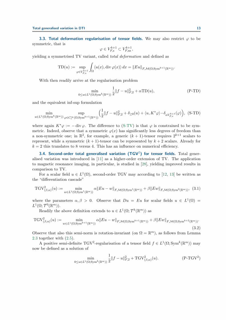
3.3. Total deformation regularisation of tensor fields. We may also restrict ϕ to besymmetric, that is
ϕ ∈ V k+1F,s ⊂ V
k+1F,ns ,
yielding a symmetrised TV variant, called total deformation and defined as
TD(u) := supϕ∈V k+1
F,s
∫Ω〈u(x), divϕ(x)〉 dx = ‖Eu‖F,M(Ω;Symk+1(Rm)).
With then readily arrive at the regularisation problem
min0≤u∈L1(Ω;Symk(Rm))
1
2‖f − u‖2F,2 + αTD(u), (P-TD)
and the equivalent inf-sup formulation
minu∈L1(Ω;Symk(Rm))
supϕ∈C∞c (Ω;Symk+1(Rm))
(1
2‖f − u‖2F,2 + δ≥0(u) + 〈u,K∗ϕ〉−δαV k+1
F,s(ϕ)), (S-TD)
where again K∗ϕ := −divϕ. The difference to (S-TV) is that ϕ is constrained to be sym-metric. Indeed, observe that a symmetric ϕ(x) has significantly less degrees of freedom thana non-symmetric one; in R2, for example, a generic (k + 1)-tensor requires 2k+1 scalars torepresent, while a symmetric (k + 1)-tensor can be represented by k + 2 scalars. Already fork = 2 this translates to 8 versus 4. This has an influence on numerical efficiency.
3.4. Second-order total generalised variation (TGV2) for tensor fields. Total gener-alised variation was introduced in [11] as a higher-order extension of TV. The applicationto magnetic resonance imaging, in particular, is studied in [28], yielding improved results incomparison to TV.
For a scalar field u ∈ L1(Ω), second-order TGV may according to [12, 13] be written asthe “differentiation cascade”
TGV2(β,α)(u) := min
w∈L1(Ω;Sym1(Rm))α‖Eu− w‖F,M(Ω;Sym1(Rm)) + β‖Ew‖F,M(Ω;Sym2(Rm)), (3.1)
where the parameters α, β > 0. Observe that Du = Eu for scalar fields u ∈ L1(Ω) =L1(Ω; T 0(Rm)).
Readily the above definition extends to u ∈ L1(Ω; T k(Rm)) as
TGV2(β,α)(u) := min
w∈L1(Ω;Symk+1(Rm))α‖Eu− w‖F,M(Ω;Symk+1(Rm)) + β‖Ew‖F,M(Ω;Symk+2(Rm)).
(3.2)Observe that also this semi-norm is rotation-invariant (on Ω = Rm), as follows from Lemma2.3 together with (2.5).
A positive semi-definite TGV2-regularisation of a tensor field f ∈ L1(Ω; Symk(Rm)) maynow be defined as a solution of
min0≤u∈L1(Ω;Symk(Rm))
1
2‖f − u‖2F,2 + TGV2
(β,α)(u). (P-TGV2)

14 T. Valkonen, K. Bredies, and F. Knoll
This can again be written in the inf-sup form
minu,w
supϕ,ψ
(1
2‖f − u‖2F,2 + δ≥0(u) + 〈(u,w),K∗(ϕ,ψ)〉−δαV k+1
F,s(ϕ)− δβV k+2
F,s(ψ)), (S-TGV2)
where u ∈ L1(Ω; Symk(Rm)), w ∈ L1(Ω; Symk+1(Rm)), ϕ ∈ C∞c (Ω; Symk+1(Rm)), and ψ ∈C∞c (Ω; Symk+2(Rm)), while the operator K∗ is defined by K∗(ϕ,ψ) := (−divϕ,−ϕ− divψ).
Remark 3.1 (Symmetric differentials). It can be argued that TGV2 defined above should becalled TGD2, for total generalised deformation, due to the use of symmetrised differentials,and the fact that TD, not TV, is the first-order equivalent of TGV2. The reason for calling(3.2) TGV is historical: TGV2 in the scalar case (3.1) already employs symmetric differentials.Of course, for scalar fields Eu = Du, and so TV and TD also agree.
It is also possible to define “non-symmetric TGV2”, bearing similar differences to “sym-metric TGV2” as TV bears to TD. We however do not do that, because such a regulariserwould be computationally much heavier, due to far greater degree of freedom, and becausewe have found the symmetric TD to offer numerically better results than TV.
3.5. Existence of solutions. We now show that the minimisation problems discussedabove admit solutions, as stated by the following theorem.
Theorem 3.1. Let Ω ⊂ Rm be a bounded Lipschitz domain, k ≥ 0, and f ∈ L2(Ω; T k(Rm)).Then (P-TV) admits a solution 0 ≤ u ∈ BV(Ω; Symk(Rm)), and (P-TD), and (P-TGV2)admit solutions 0 ≤ u ∈ BD(Ω; Symk(Rm)).
Proof. The proof for (P-TV) and (P-TD) is quite standard; cf., e.g., [26]. Indeed, letui ≥ 0∞i=0 ⊂ L1(Ω; Symk(Rm)) be a minimising sequence for (P-TD). Observe that
supi‖ui‖F,2 + ‖Eui‖F,M(Ω;Symk+1(Rm)) <∞. (3.3)
Therefore, as in the case of scalar functions, we deduce that there exists a subsequence,unrelabelled, and 0 ≤ u ∈ BD(Ω; Symk(Rm)), such that ui u weakly in L2(Ω; T k(Rm)),and Eui ∗ Eu weakly* inM(Ω; Symk+1(Rm)). Lower semi-continuity of ‖·‖F,M(Ω;Symk+1(Rm))
and of ‖ · ‖F,2 now shows that u is a solution to (P-TD).The claim for (P-TV) follows analogously in BV(Ω; Symk(Rm)), with Eu replaced by Du
above.It remains to show the existence of a solution 0 ≤ u ∈ BD(Ω; Symk(Rm)), u ≥ 0, to
(P-TGV2). As in the scalar case k = 0, considered in [13], we need to show that for somec > 0 it holds
c(‖u‖F,1 + ‖Eu‖F,M(Ω;Symk+1(Rm))
)≤ ‖u‖F,1 + TGV2
(β,α)(u), (u ∈ L1(Ω; Symk(Rm)), (3.4)
and that TGV2(β,α) is lower semi-continuous with respect to weak* convergence of Eui to
Eu. These results are contained in the following two lemmas. We let then ui ≥ 0∞i=1 ⊂L1(Ω; Symk(Rm)) be a minimising sequence for (P-TGV2). We want to show that (3.3) holds.Indeed, supi ‖ui‖F,1 <∞ thanks to Ω being bounded and
supi‖f − ui‖F,2 + TGV2
(β,α)(ui) <∞, (3.5)

Total generalised variation in DTI 15
the latter following from ui being a minimising sequence for (P-TGV2). It now follows from(3.4) that supi ‖Eui‖F,M(Ω;Symk+1(Rm)) < ∞. This and (3.5) lead to (3.3). The same argu-
ments as above now provide 0 ≤ u ∈ BD(Ω; Symk(Rm)), and lower semi-continuity establishesthat it solves (P-TGV2).
Lemma 3.2. Let Ω ⊂ Rm be a bounded Lipschitz domain and k ≥ 0. Then there existconstants c, C > 0, dependent on Ω, k,m, such that for all u ∈ L1(Ω; Symk(Rm)) it holds
c‖u‖BD(Ω;Symk(Rm)) ≤ ‖u‖F,1 + TGV2(β,α)(u) ≤ C‖u‖BD(Ω;Symk(Rm)). (3.6)
Proof. The proof is a straightforward extension of the equivalence proof for k = 0 in [13],employing the tensor Sobolev-Korn estimates from [10]. Indeed, by definition
‖u‖F,1 + TGV2(β,α)(u) ≤ ‖u‖F,1 + α‖Eu− w‖F,M(Ω;Symk+1(Rm)) + β‖Ew‖F,M(Ω;Symk+2(Rm)),
for all w ∈ L1(Ω; Symk+1(Rm)), so setting w = 0 gives
‖u‖F,1 + TGV2(β,α)(u) ≤ ‖u‖F,1 + α‖Eu‖F,M(Ω;Symk+1(Rm)) ≤ C‖u‖BD(Ω;Symk(Rm))
for C = max1, α. Thus the second inequality of (3.6) holds.For the first inequality of (3.6), we may assume that Eu ∈ M(Ω; Symk+1(Rm)), since
otherwise ‖Eu−w‖F,M(Ω;Symk+1(Rm)) =∞ for all w ∈ L1(Ω; Symk+1(Rm)), and the inequalityholds trivially. We want to show that there exists C1 > 0 such that
‖Eu‖F,M(Ω;Symk+1(Rm)) ≤ C1
(‖u‖F,1 + ‖Eu− w‖F,M(Ω;Symk+1(Rm))
)(3.7)
for every u ∈ BD(Ω; Symk(Rm)) and w ∈ L1(Ω; Symk+1(Rm)) satisfying Ew = 0, i.e.,w ∈ kerE. For the proof of the fact that E has a non-trivial finite-dimensional kernel,see [10]. Indeed, suppose that (3.7) does not hold. Then there exist sequences ui∞i=0 ⊂BD(Ω; Symk(Rm)) and wi∞i=0 ⊂ L1(Ω; Symk+1(Rm)) ∩ kerE such that for i = 1, 2, 3, . . ., itholds
‖Eui‖F,M(Ω;Symk+1(Rm)) = 1 and ‖ui‖F,1 + ‖Eui − wi‖F,M(Ω;Symk+1(Rm)) ≤ 1/i, (3.8)
It follows that ui → 0 strongly in L1(Ω; Symk(Rm)). Consequently Eui ∗ 0 weakly* inthe space M(Ω; Symk+1(Rm)). Employing the first half of (3.8) in the second, it moreoverfollows that supi ‖wi‖F,1 < ∞. Since kerE is finite-dimensional, we deduce that there existsa convergent subsequence, unrelabelled, and w ∈ L1(Ω; Symk+1(Rm))∩kerE, such that wi →w strongly in L1(Ω; Symk+1(Rm)). It hence follows from (3.8) that Eui → w strongly inM(Ω; Symk+1(Rm)). But Eui ∗ 0, so w = 0. This means that ‖Eui‖F,M(Ω;Symk+1(Rm)) → 0
in contradiction to (3.8). Hence (3.7) holds.Now we employ from [10] the following Sobolev-Korn estimate: there exists C2 > 0 such
that for all w ∈ BD(Ω; Symk+1(Rm)) there exists w ∈ L1(Ω; Symk+1(Rm)) ∩ kerE satisfying
‖w − w‖F,1 ≤ C2‖Ew‖F,M(Ω;Symk+2(Rm)).

16 T. Valkonen, K. Bredies, and F. Knoll
For this choice of w, we deduce the existence of C3 > 0 such that for all u ∈ BD(Ω; Symk(Rm))and w ∈ BD(Ω; Symk+1(Rm)) it holds
‖Eu− w‖F,M(Ω;Symk+1(Rm)) ≤ ‖Eu− w‖F,M(Ω;Symk+1(Rm)) + ‖w − w‖F,1≤ C3
(α‖Eu− w‖F,M(Ω;Symk+1(Rm)) + β‖Ew‖F,M(Ω;Symk+2(Rm))
).
Employing this estimate in (3.7) yields for some C4 > 0 the estimate
‖u‖BD(Ω;Symk(Rm)) ≤ C4
(‖u‖F,1 + α‖Eu− w‖F,M(Ω;Symk+1(Rm)) + β‖Ew‖F,M(Ω;Symk+2(Rm))
),
which holds for all w ∈ BD(Ω; Symk+1(Rm)) and u ∈ BD(Ω; Symk(Rm)). Hence the firstinequality of (3.6) holds with c = C−1
4 .Lemma 3.3. Let Ω ⊂ Rm be a bounded Lipschitz domain and k ≥ 0. Then the function
F (µ) := minw∈L1(Ω;Symk+1(Rm))
α‖µ− w‖F,M(Ω;Symk+1(Rm)) + β‖Ew‖F,M(Ω;Symk+2(Rm)),
where µ ∈M(Ω; Symk+1(Rm)), is lower semi-continuous with respect to weak* convergence.Proof. Let µi ∗ µ weakly* inM(Ω; Symk+1(Rm)). Observe that by the Banach-Steinhaus
theorem, supi ‖µi‖F,M(Ω;Symk+1(Rm)) <∞. Consequently also supi F (µi) <∞.
We first establish that F (µi) admits a minimiser wi ∈ BD(Ω; Symk+1(Rm)). Indeed,let vj∞j=0 ⊂ BD(Ω; Symk+1(Rm)) be a minimising sequence for F (µi). The sequence is
obviously bounded in BD(Ω; Symk+1(Rm)). Thus [10, Theorem 4.17], establishes that thereexists a subsequence, unrelabelled, convergent strongly in L1(Ω; Symk+1(Rm)) to some v ∈L1(Ω; Symk+1(Rm)). A standard argument (cf., e.g, [4, Proposition 3.13]) establishes thatEvi ∗ Ev weakly* in M(Ω; Symk+2(Rm)). Finally, lower semi-continuity yields that wi := vminimises F (µi).
Knowing that F (µi) admits a minimiser for each i = 0, 1, 2, . . ., we now establish lowersemi-continuity. Since supi F (µi) + ‖µi‖F,M(Ω;Symk+1(Rm)) <∞, we deduce that
supi‖wi‖F,1 + ‖Ewi‖F,M(Ω;Symk+2(Rm)) <∞.
Hence some subsequence of wi∞i=0 converges weakly in BD(Ω; Symk(Rm)) to some w ∈BD(Ω; Symk(Rm)). By lower semi-continuity of norms we deduce that
F (µ) ≤ α‖µ− w‖F,M(Ω;Symk+1(Rm)) + β‖Ew‖F,M(Ω;Symk+2(Rm)),
≤ lim infi→∞
α‖µi − wi‖F,M(Ω;Symk+1(Rm)) + β‖Ewi‖F,M(Ω;Symk+2(Rm)) = lim infi→∞
F (µi).
This establishes the lower semi-continuity of F .Remark 3.2 (Dual-ball formulation). If we extended to the tensor case the equivalence proof
[12, 13] of the differentiation cascade formulation (3.1) of TGV2(β,α), and the original dual-ball
formulation
TGV2(β,α)(u) := sup
∫Ωudiv2 ϕdx
∣∣∣ ϕ ∈ C2c (Ω; Sym2(Rm)), ‖v‖F,∞ ≤ β, ‖div v‖F,∞ ≤ α
,

Total generalised variation in DTI 17
then, following the original proof in [11], we could almost trivially obtain lower semi-continuityof TGV2
(β,α) with respect to convergence in Lp. This would imply weak lower semi-continuity
in L1, and could be used to replace Lemma 3.3 in the proof of Theorem 3.1. The equivalenceproof is, however, very long, and not our focus here, so we do not provide the extension, andchoose to work entirely with the differentiation cascade formulation, that is more practical inthe numerical methods of our choosing.
4. Algorithmic aspects. We now move on to discuss the algorithmic aspects of the solu-tion of the regularisation problems above. We do this through the saddle-point formulations.
4.1. Discretisation and the algorithm. The problems (S-TV), (S-TD), and (S-TGV2)are of the form
infx
supyG(x) + 〈x,K∗y〉−F ∗(y)
for proper convex lower semi-continuous G,F ∗. This suggests that the Chambolle-Pock al-gorithm [15] could be applied. A problem with the original infinite-dimensional problems is,however, that a (pre)conjugate of K∗ cannot easily be defined, as the spaces involved arenot reflexive; in the case of TV, in particular K∗ : C∞c (Ω; T k+1(Rm)) → C∞c (Ω; T k(Rm)).In practise the algorithm is applied on finite dimensional discretisations, however, and thisproblem does not surface when the discretisations are chosen suitably. We choose to representeach tensor field f , u, w, ϕ and ψ by values on an uniform grid, and discretise K∗ by forwarddifferences, yielding the operator K∗h. We then take Kh := (K∗h)∗ as the discrete conjugate ofK∗h.
For TD and TV the function
G(u) = G0(u) :=1
2‖f − u‖2F,2 + δ≥0(u).
is uniformly convex. We therefore describe the accelerated version of the Chambolle-Pockalgorithm. It has the following assumptions.
Assumption 4.1. Consider the problem
minx
maxyG(x) + 〈x,K∗hy〉−F ∗(y),
where Kh : X → Y is a continuous linear operator between the finite-dimensional Hilbert-spaces X and Y , and G : X → [0,+∞] and F ∗ : Y → [0,+∞] are proper, convex and lowersemi-continuous, with F ∗ the conjugate of a convex lower semi-continuous function F . Let,moreover, γ ≥ 0 be such that for any x ∈ dom ∂G it holds
G(x′)−G(x) ≥ 〈z, x′ − x〉+γ
2‖x− x′‖2 for all z ∈ ∂G(x), x′ ∈ X.
Algorithm 4.1. Suppose Assumption 4.1 is satisfied. Following [15], perform the steps:
1. Pick τ0, σ0 > 0 satisfying τ0σ0‖Kh‖2 ≤ 1, as well as (x0, y0) ∈ X × Y . Set x0 = x0.

18 T. Valkonen, K. Bredies, and F. Knoll
2. For i = 0, 1, 2, . . ., repeat the following updates until a stopping criterion is satisfied.
yi+1 := (I + σi∂F∗)−1(yi + σiKhx
i)
xi+1 := (I + τi∂G)−1(xi − τiK∗hyi+1)
θi := (1 + 2γτi)−1/2, τi+1 := θiτi, σi+1 := σi/θi
xi+1 := xi+1 + θi(xi+1 − xi).
For TD and TV we have γ = 1. For TGV2 we should in take γ = 0, because G(u,w) =G0(u) does not depend on w, and is thus not uniformly convex. In this case the abovealgorithm reduces to the unaccelerated version that does not update θi and σi. In numericalpractise γ = 1 works often better, but at other times does not converge.
The resolvent operators that need to be calculated to obtain xi+1 and yi+1, may be written
(I + τ∂G)−1(x) = arg miny
‖x− y‖2
2τ+G(y)
.
The efficient realisation of Algorithm 4.1 depends on the efficient realisation of these minimi-sation problems. In our primary case of interest with k = 2, it turns out that they reduce toeasily calculable projections, as follows.
We begin by considering (S-TV). First, for F ∗(ϕ) = δαV k+1F,s
(ϕ), the resolvent is
(I + σ∂F ∗)−1(v) = arg minϕ
‖v − ϕ‖2F,22σ
+ δαV k+1F,s
(ϕ)
.
This reduces to a pointwise projection
ϕ(x) = P‖·‖F≤α(v(x)) = v(x) min1, α/‖v(x)‖F (4.1)
for all x ∈ Ω. Secondly, G = G0, for which we solve
[(I + τ∂G0)−1(v)](x) = P≥0
(v(x) + f(x)τ
1 + τ
), (x ∈ Ω). (4.2)
The pointwise projection
P≥0(A) := min0≤X∈Sym2(Rm)
‖A−X‖2F , (A ∈ Sym2(Rm)),
can be performed by projecting each eigenvalue of A to R+. (This can be seen from thestructure of the normal cone N≥0(x′), spelled out in, e.g., [42, Lemma 3.1]. See also [31] forrelated eigenvalue projection results that are useful for dealing with the nuclear and spectralnorms.)
Regarding (S-TD), still G = G0, so we get the resolvent (4.2). Also for F ∗ the resolvent
(I + σ∂F ∗)−1(v) = arg minϕ
‖v − ϕ‖2F,22σ
+ δαV k+1F,ns
(ϕ)

Total generalised variation in DTI 19
has the same solution (4.1) as in the case of (S-TV).
It remains to consider the resolvents for (S-TGV2). Minding that G(u,w) = G0(u), wefind that
(I + τ∂G)−1(v, q) = ((I + τ∂G0)−1(v), q).
Likewise, from the expression
F ∗(ϕ,ψ) = δαV k+1F,s
(ϕ) + δβV k+2F,s
(ψ),
we immediately deduce that
(I + σ∂F ∗)−1(v, q) = (ϕ,ψ),
with the projection (4.1) applied on ϕ and ψ separately; more precisely ϕ(x) = P‖·‖F≤α(v(x))and ψ(x) = P‖·‖F≤β(q(x)).
4.2. Duality gap as stopping criterion. For (S-TV) and (S-TD) it poses no difficulty tocalculate the duality gap
F (Khu) +G(u) +G∗(−K∗hϕ) + F ∗(ϕ),
and to use the reduction of the duality gap beyond a certain threshold as a stopping criterion.Regarding (S-TGV2), the variable w from the expression TGV2(u) = minw α‖Eu − w‖ +β‖Ew‖ does not appear in G(u,w) = G0(u), yielding G∗(a, b) = G∗0(a) + δ0(b). The resultis that in practise G∗(a, b) =∞ in the algorithm, so the duality gap as such is not useful fora stopping criterion.
If we had an a priori bound M on ‖w‖F,1, at an optimal solution (u, w), then we could addthe term δB(0,M)(‖w‖F,1) to G, resulting in practical G∗ and duality gap. It can be shown (seeProposition A.1 in the Appendix) that such a bound indeed exists. Unfortunately, however,due to the nature of the proof, we only know the existence, but not the exact magnitude.
Fortunately it turns out that we can also pick M a posteriori, because if M is largeenough, δB(0,M)(‖w‖F,1) vanishes in Algorithm 4.1, and therefore, if the duality gap becomesinfinite, we can simply increase M , which is only used to calculate the duality gap/stoppingcriterion. This suggests to employ the following generic algorithm, where for TGV2 we havexi = (ui, wi), yi = (ϕi, ψi), and
U := (u,w) ∈ L1(Ω; Symk(Rm))× L1(Ω; Symk+1(Rm)) | ‖w‖F,1 ≤ 1.
The idea is that we always decrease the duality gap of the modified problem, where G isreplaced by G(x) + δMU (x), for some M > 0, unknown a priori, by a given fraction ρ, chosena priori.
Algorithm 4.2. Suppose Assumption 4.1 holds, and that U ⊂ X has non-empty interior.In each step of the Algorithm 4.1, perform the following additional operations.
1. Pick ρ ∈ (0, 1) and M0 ≥ 0. Define
Gi(x) := G(x) + δMiU (x).

20 T. Valkonen, K. Bredies, and F. Knoll
2. Update the variables as in Algorithm 4.1 with G = Gi. Pick Mi+1 ≥Mi large enoughthat x ∈Mi+1U . Calculate the initial and current pseudo-duality gaps
di+10 := F (Khx
0) +Gi+1(x0) +G∗i+1(−K∗hy0) + F ∗(y0),
di+1 := F (Khxi+1) +Gi+1(xi+1) +G∗i+1(−K∗hyi+1) + F ∗(yi+1).
If di+1 < ρdi+10 , finish execution of the algorithm, with the solution (xi+1, yi+1). Oth-
erwise continue iteration.Remark 4.1 (Computations on 2D slices of 3D data). The mathematical theory on tensor
fields above, in particular the definition (2.2) of the tensor divergence, only applies to tensorsfields f : Ω → Symk(Rm), where the domain Ω ⊂ Rm has the same dimension m as thetensor parameters. Therefore, it is not directly possible to do computations on 2D slices of 3Dtensor fields f : Ω ⊂ R2 → Sym2(R3). For reasons of computational efficiency, working on 2Dslices of data instead of the full 3D volume can sometimes however be desirable. A solutionis to assume that the full image is constant in the z direction, and work on the extensionf3D(x, y, z) = f(x, y). At the level of the numerical implementation this extension can bereduced to performing 3D calculations on the slice f , taking the differentials in the z directionas zero.
5. Numerical results. We will now numerically study the performance of the different reg-ularisation models on a synthetic test data, as well as an in-vivo brain measurement. We firstdiscuss how the results are reported, followed by discussing in detail how the computationalalgorithm is parametrised. We then describe how our synthetic test data is constructed, and,and finally represent and analyse the results for both this synthetic test data and an in-vivobrain measurement.
5.1. Error measures. We would like to have a numerical value for the quality of thesolution, compared to noise-free test data. An obvious candidate is, of course, the Frobenius-L2 norm
dF (f, u) := ‖f − u‖F,2.
This distance is, however, difficult to interpret in geometric terms directly related to f and u.Therefore we introduce three other error measures that measure different geometrical aspectsof the tensors.
As the first geometrical error measure we have the L2 norm
dA(f, u) := ‖FAf − FAu‖L2(Ω)
of the differences of the fractional anisotropies, defined by
FAu(x) =(∑m
i=1(λi − λ)2)1/2(∑m
i=1 λ2i
)−1/2∈ [0, 1], (x ∈ Ω),
where λ1, . . . , λm are the eigenvalues of u(x), and λ =∑m
i=1 λi/m. The second geometricalerror measure is the L2 norm
dλ(f, u) := ‖λu − λf‖L2(Ω)
Total generalised variation in DTI 21
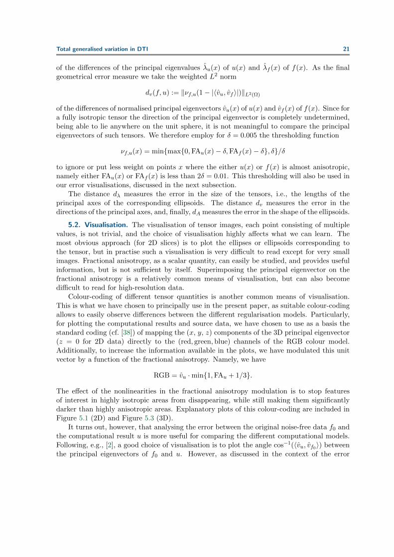
of the differences of the principal eigenvalues λu(x) of u(x) and λf (x) of f(x). As the finalgeometrical error measure we take the weighted L2 norm
dv(f, u) := ‖νf,u(1− |〈vu, vf 〉|)‖L2(Ω)
of the differences of normalised principal eigenvectors vu(x) of u(x) and vf (x) of f(x). Since fora fully isotropic tensor the direction of the principal eigenvector is completely undetermined,being able to lie anywhere on the unit sphere, it is not meaningful to compare the principaleigenvectors of such tensors. We therefore employ for δ = 0.005 the thresholding function
νf,u(x) = minmax0,FAu(x)− δ,FAf (x)− δ, δ/δ
to ignore or put less weight on points x where the either u(x) or f(x) is almost anisotropic,namely either FAu(x) or FAf (x) is less than 2δ = 0.01. This thresholding will also be used inour error visualisations, discussed in the next subsection.
The distance dλ measures the error in the size of the tensors, i.e., the lengths of theprincipal axes of the corresponding ellipsoids. The distance dv measures the error in thedirections of the principal axes, and, finally, dA measures the error in the shape of the ellipsoids.
5.2. Visualisation. The visualisation of tensor images, each point consisting of multiplevalues, is not trivial, and the choice of visualisation highly affects what we can learn. Themost obvious approach (for 2D slices) is to plot the ellipses or ellipsoids corresponding tothe tensor, but in practise such a visualisation is very difficult to read except for very smallimages. Fractional anisotropy, as a scalar quantity, can easily be studied, and provides usefulinformation, but is not sufficient by itself. Superimposing the principal eigenvector on thefractional anisotropy is a relatively common means of visualisation, but can also becomedifficult to read for high-resolution data.
Colour-coding of different tensor quantities is another common means of visualisation.This is what we have chosen to principally use in the present paper, as suitable colour-codingallows to easily observe differences between the different regularisation models. Particularly,for plotting the computational results and source data, we have chosen to use as a basis thestandard coding (cf. [38]) of mapping the (x, y, z) components of the 3D principal eigenvector(z = 0 for 2D data) directly to the (red, green,blue) channels of the RGB colour model.Additionally, to increase the information available in the plots, we have modulated this unitvector by a function of the fractional anisotropy. Namely, we have
RGB = vu ·min1,FAu + 1/3.
The effect of the nonlinearities in the fractional anisotropy modulation is to stop featuresof interest in highly isotropic areas from disappearing, while still making them significantlydarker than highly anisotropic areas. Explanatory plots of this colour-coding are included inFigure 5.1 (2D) and Figure 5.3 (3D).
It turns out, however, that analysing the error between the original noise-free data f0 andthe computational result u is more useful for comparing the different computational models.Following, e.g., [2], a good choice of visualisation is to plot the angle cos−1(〈vu, vf0〉) betweenthe principal eigenvectors of f0 and u. However, as discussed in the context of the error

22 T. Valkonen, K. Bredies, and F. Knoll
measures in the previous subsection, this error is meaningless for fully anisotropic tensors.Therefore we use the same thresholding νf,u as in the definition of dv to put less weight onsuch points, and plot
θ = νf0,u cos−1(〈vu, vf0〉).
using the “jet” colour map of Matlab, spanning from blue through cyan and yellow to red.This colour coding does not yet describe errors eFA = |FAu − FAf0 | in reconstruction of
fractional anisotropy, and therefore we have chosen to plot that as well, using shades of grey,so that the resulting RGB (red, green, blue) value of an image pixel is the componentwisemaximum of the two colours,
RGB = maxjet(min1, 2θ/π),min1, eFA/0.15.
The minimum expressions serve to compress the colours for high errors. A clarifying plot ofthe colour-coding is included in Figures 5.2 and 5.4.
5.3. The evaluated models. We evaluate the models (P-TD), (P-TV), and (P-TGV2),applying algorithm Algorithm 4.2 to solve each of them, as discussed in the preceding sections.Moreover, we study the log-Euclidean [5, 6, 20] regularisation
minu≥0
1
2‖ log f − log u‖2 + αTV(log u). (P-logTV)
In practise this is implemented by taking u = exp v where v solves minv12‖ log f−v‖2+αTV(v).
This can be calculated with Algorithm 4.2 again, just like normal TV, but without the positivedefiniteness constraint. However, we have the minor problem that log f(x) =
∑mi=1 λi(vi⊗ vi)
has complex values when f(x) is not positive definite, i.e, has a non-positive eigenvalue λi.In principle we could calculate the distance | log f(x) − log u(x)| in the complex sense. But,by the theory of log-Euclidean metrics, the boundary of the positive definite cone should beinfinitely far from any positive definite tensor. Therefore, in practise, when such data occurs,we replace λi by a small positive number ε > 0 for the calculation of log f(x).
In addition to the models (P-TD), (P-TV), (P-TGV2), and (P-logTV), for numericalexperiments on in-vivo data we evaluate for comparison the more conventional approach ofdenoising each DWI image separately [1]. Following [29], we perform this by total variationregularisation, i.e., solving (P-TV) for k = 0 by Algorithm 4.2 for each of the DWI measure-ments. The reported iteration count for this regularisation model, denoted DWITV, will bethe maximum over the different DWI measurements.
For each evaluated model we pick Algorithm 4.2 as the numerical method. As the stoppingcriterion we use the normalised duality gap ρ = 0.001, and additionally limit the number ofiterations to at most 5000. The initial iterates are always x0 = 0, y0 = 0.
For (P-TGV2) we take τ0 = σ0 = 0.95/√L′1, where L′h = (16+h2+
√h4 + 32h2)/(2h2) is a
bound on the squared norm ‖K∗h‖22 of the discretisationK∗h ofK∗(ϕ,ψ) := (−divϕ,−ϕ−divψ)on a grid of cell width h (for domains Ω ⊂ R2!). At each iteration we update Mi+1 :=‖wi+1‖F,1.
For (P-TV), (P-TD), and (P-logTV) we take, likewise, τ0 = σ0 = 0.95/√L1, where this
time Lh = 8/h2 bounds ‖∇‖22 on a grid of cell width h on domains Ω ⊂ R2; see [14].

Total generalised variation in DTI 23
5.4. Choice of regularisation parameter. The choice of the regularisation parameters αand β highly affects the denoising results, and care has to be taken to make the comparisonof different denoising models fair. One possibility would be to find the “best” parameters foreach model, and compare these results. The choice of “best” is, however, not a trivial one,especially as in clinical data features that are difficult to quantify can be more important thansimple error measures.
Moreover, we find that it is important to compare the sensitivity of the models to pa-rameter choice, and to study the range of denoising results achievable with each model. Wetherefore report denoising results of each model for two different choices of the regularisationparameters. We call them the “large parameter choice” and the “small parameter choice”.In each test case, we pick for each regularisation model H a parameter α0(H) by trial anderror. For the large parameter choice we then set for each model α = α0(H) and, for TGV2,β = 10α0(TGV2). For the small parameter choice we set α = 0.4α0(H), and for TGV2,β = 0.6α0(TGV2). Observe that in this case α+β = α0(TGV2), which is a heuristic we wantto test for TGV2 against TV and TD.
Indeed, we pick α0(TV) = α0(TD) = α0(TGV2). For the large parameter choice this isclearly fair: When β approaches infinity, the only real difference between the functionals istheir kernel. For TV it is constant functions, for TD it is “infinitesimal rigid displacements”[10], i.e., functions u such that Eu = 0, and for TGV2 it is functions u such that the absolutelycontinuous part w of Eu satisfies Ew = 0. For the small parameter choice, we will justify thechoice of same α0(H) numerically.
For H = logTV,DWITV we pick by trial and error another α0(H) that seems to provideresults comparable to TV, TD and TGV2 for both the large and small parameter choices. Forour tests with in-vivo brain data, for H = TV,TD,TGV2 we end up in practise picking
α0(H) = α0µ, µ := ‖maxiλi(f0(x))‖L∞(Ω),
for a single “base regularisation parameter” α0 found by trial and error, and the maximumeigenvalue µ of f0. For logTV we have then often found
α0(logTV) = α0| logµ|, (5.1)
to be a good choice, and for DWITV
α0(DWITV) = α0‖meanbAb(x)‖L∞(Ω).
These rather simple choices are somewhat justified by the fact that the factor between α0 andα0(H) is in each case computed by an analogous rule on the data, minding that logTV doesTV regularisation on log(f0). For our experiments on synthetic test data, we however haveended up choosing
α0(logTV) = 2α0| logµ|, (5.2)
which we have found by trial and error to be fairer than (5.1), although the scale of the latterchoice is also right, and the computational results not foo far from TV, TD, and logTV.
Although it is difficult to do complete justice to all the models, we believe to have chosenthe parameters reasonably fairly. Given that we report results of all models for two parameterchoices, we are able to observe trends that are relatively independent of parameter choice.

24 T. Valkonen, K. Bredies, and F. Knoll
5.5. Synthetic data. Our noise-free synthetic test data consists of a 128 × 128 imageof Sym2(R2) tensors, divided into four smaller rectangles each having a tensor field withdifferent properties; Figure 5.1(e) contains an illustration. The origin (0, 0) of the image is inthe lower-right corner.
In the rectangle (64, 128)× (64, 128) we have the constant tensors
f0(x, y) =
[1.1 00 0.9
].
(We avoid the identity tensor due to ambiguity of a principal eigenvector.) This region isin the kernel of both differential operators D and E. Next there is a lower-left rectangle(0, 64)× (0, 64) consisting of an affine tensor field
f0(x, y) = I + 0.005
([0 11 2
](x− 1) +
[−2 −1−1 0
](y − 1)
).
In this region Ef0 = 0 but Df0 6= 0. Then, we have the upper-left rectangle (0, 64)× (64, 128)that has an affine tensor field
f0(x, y) = I + 0.02
([1 00 0
](x− 1) +
[0 00 1
](y − 65)
).
In this region both Df0 6= 0 and Ef0 6= 0. Finally, in the lower-right rectangle (64, 128) ×(0, 64), we have the non-linear tensor field
f0(x, y) = Rx
[3/4 00 1/2
]RTx , Rx :=
[1 00 1
]cos
(π
2
x− 65
64
)+
[0 −11 0
]sin
(π
2
x− 65
64
),
rotating the tensor 34e1⊗e1 + 1
2e2⊗e2 by an angle between [0, π/2] as the x-coordinate varies.
5.6. The Stejskal-Tanner equation and Rician noise. A diffusion tensor D ∈ Sym2(R3)at a given voxel of a diffusion tensor image produced through DWI measurements is governedby the Stejskal-Tanner equation
Ab = A0 exp(−〈b,D〉). (5.3)
Here the b matrix parametrises a diffusion gradient, and Ab is the DWI measurement corre-sponding to b. At least K ≥ 6 independent non-zero diffusion gradients are needed to solvefor D by regression from the measurements A0, Ab1 , . . . , AbK; see, e.g., [8].
The noise in the DWI measurements Abi is Rician; see, e.g., [23]. We wish to apply thesame noise model on our synthetic test data as well. By choosing the b-matrices suitably,we can extract each individual component of D, and therefore apply Rician noise on eachcomponent separately
Dij = log(ricernd(exp(Dij), σ)),
where σ parametrises the Rice distribution, and ricernd is a Matlab function that appliesrandom Rician noise.

Total generalised variation in DTI 25
5.7. Results on synthetic data. To the synthetic noise-free test data f0, we apply Riciannoise with the parameter σ = 0.15, yielding the noisy test data f with PSNR ≈ 34.4 dB (inthe DWI domain with exponential relationship to the tensor field). The maximal eigenvalueof the test data f0, affecting the regularisation parameters, is µ ≈ 2.3. We have chosen thebase regularisation parameter α0 = 0.25 by trial and error and the rule (5.2) for logTV. Theresults of applying the denoising models described above on f are depicted in Figure 5.1, andthe error maps in Figure 5.2.
Our principal observations are the following. Firstly, in the top-left region, where u belongsto (kerE)c, TGV2 is best at restoring the diagonal line between the red and green-colouredregions for the large parameter choice. TV and logTV display a quite prominent S-shape: thediagonal bends downwards on the right and upwards on the left. For TD the reconstructionof the diagonal is quite noisy. We, however, note that the fact these effects can be seen is aresult of the non-linearities in our visualisation; if the principal eigenvector were modulated bythe fractional anisotropy directly, i.e., if vuFAu were plotted, this S-shape could not be seen,as on the diagonal the tensors are fully isotropic, and the region around the diagonal wouldblend to black without the jump. What happens in our test data across the diagonal is thatthe principal eigenvector switches from pointing horizontally to pointing vertically. It appearsthat TGV2 restores such extremely sensitive differences better than the other regularisationmodels. Although for the small parameter choice not so much differences can be seen alongthe diagonal in Figure 5.1, studying Figure 5.2 we observe that the reconstruction error is forboth parameter choices quite noisy around the diagonal for the first-order models, while forTGV2 it is relatively flat.
Secondly, in the top-right region, where u belongs to kerD, we observe, by contrast, thatfor the small parameter choice TV is best at restoring the flatness of this region. Presumablythe stair-casing effect helps here.
In the bottom-left region, where u belongs to kerE \kerD, the differences between TGV2,TD, and TV are again minor; studying Figure 5.2, we see, however, that TV exhibits slightlymore noisy errors, while logTV exhibits in general more noise in this region.
Indeed, in the nonlinear bottom-right region, we observe that logTV is extremely noisy forboth parameter choices. For the smaller parameter choice all the methods are somewhat noisyin this region. Studying Figure 5.2, we see that it has large errors in fractional anisotropy.Looking at the error score dA superimposed on Figure 5.1, we see indeed that logTV has higherrors in fractional anisotropy, a trend that we will also see in tests with in-vivo brain data.It could be argued that the regularisation parameter should be higher. We tried to increaseit by a factor of two, but the S-shape become even more prominent and dF increased, withthe errors disappearing. We also expected some stair-casing effect for the first order methodsin this region, but it is not noticeable. Only in the error plot of Figure 5.2 do we see it.
Concerning iteration counts (also superimposed on Figure 5.1), we observe TGV2 for thelarge parameter choice has required 14 times as much iterations as the other models, and forthe smaller parameter choice also 1.5 times as many. It however provides clearly the bestresults for the large parameter choice, by the error scores as well (superimposed on Figure5.1). For the small parameter choice TV can be said to provide better results, but neither isso good as TGV2 for the large parameter choice.
Finally, we note that the error measures superimposed on Figure 5.1(b3) are comparable

26 T. Valkonen, K. Bredies, and F. Knoll
to those on (a1) and (a4). This suggests that while visually (b3) is worse, from the pointof view of error measures the heuristic choice of α + β for TGV2 equal to α for TV or TD,as discussed in Subsection 5.4, seems at least as reasonable as choosing the same α for allthe models and a large β. This suspicion is however not confirmed by the following tests onin-vivo brain data, and indeed the choice of α seems more important than β.
5.8. In-vivo brain data. Finally, we apply the regularisation models to a clinical in-vivo diffusion tensor image of a human brain. The measurements for our test data set wereperformed on a clinical 3T system (Siemens Magnetom TIM Trio, Erlangen, Germany), usinga 32 channel head coil. Written informed consent was obtained from all volunteers beforethe examination. A 2D diffusion weighted single shot EPI sequence with diffusion sensitisinggradients applied in 12 independent directions (b = 1000s/mm2) and an additional referencescan without diffusion was used with the following sequence parameters: TR = 7900ms,TE = 94ms, flip angle 90, matrix size 128 × 128, 60 slices with a slice thickness of 2mm, inplane resolution 1.95mm× 1.95mm, 4 averages, GRAPPA acceleration factor 2. Prior to thereconstruction of the diffusion tensor, eddy current correction was performed with FSL [36].Given the four averages of 12 independent diffusion gradients, plus the zero gradient, we havealtogether 52 different DWI measurements.
When acquiring diffusion weighted MRI data, there is always a tradeoff between SNR,the imaged field of view, spatial resolution and measurement time. From a clinical point ofview, it would be extremely desirable to be able to obtain DTI data sets with whole braincoverage and an isotropic spatial resolution of approximately 1mm3. However, clinical scanprotocols are limited in measurement time to approximately 5 minutes for a diffusion weightedacquisition [38]. The reason for this is patient comfort, the required patient throughput in aclinical facility, as well as the inability to hold completely still for longer periods of time. Thisis of special importance for diffusion weighted imaging, as it is a technique that is prone toartifacts from patient movement.
Our data set is of rather high fidelity at the expense of low resolution. It is therefore suit-able as a “ground truth” or “gold standard” to which additional noise is applied, and againstwhich the results of denoising the noisy data are compared. For reasons of visualisational andcomputational practicality, we perform computations only on a single slice of the data set.The data f0 is thus a 128 × 128 image of Sym2(R3) tensors, to which the considerations inRemark 4.1 apply. We apply Rician noise with both the parameters σ = 10 (“low-noise case”,PSNR ≈ 29.0 dB) and σ = 50 (“high-noise case”, PSNR ≈ 14.5 dB) on the original DWImeasurements, before the diffusion tensors are extracted from the Stejskal-Tanner equation(5.3). Regarding regularisation parameter, the maximal eigenvalue of the data µ ≈ 0.0042,and we have by trial and error chosen the “base regularisation parameter” α0 = 0.05 for thelow-noise case and α0 = 0.15 for the high-noise case. The regularisation parameter for logTVis chosen as (5.1).
The computational results for the low-noise case are presented in Figure 5.3, and the errormaps in Figure 5.4. The results for the high-noise case are presented in Figure 5.5 and the errormaps in Figure 5.6. The results have been zoomed-in on the area (16, 112) × (16, 112), andpoints where the average DWI signal intensity is less than 10% of the mean over the wholeimage, have been masked out. Additionally, for the high-noise case, we include in Figure

Total generalised variation in DTI 27
5.7 a plot of the fractional anisotropy superimposed with the projections of the principaleigenvectors to the (x, y)-plane, for region (55, 73)×(74, 92) of the data, containing the corpuscallosum; the region is marked with a rectangle in Figure 5.5. For the low-noise case this plotis not included, because any differences between most of the methods are hard to observe.
5.9. Analysis of the low-noise case. We first study the low-noise case. From Figure 5.3it is difficult to observe any significant differences between the models, except that TV andlogTV exhibit stair-casing. Another noticeable aspect is that TGV2 requires significantly moreiterations to reach the target normalised duality gap than the other models. Nevertheless, allthe models manage to remove the additional Rician noise to some degree: Compared to thenoisy data f , the error measures (superimposed on Figure 5.3) are reduced significantly by allmodels, with the exception of the error dv in the directions of the principal eigenvectors. Incontrast to the situation with the synthetic data, where TGV2 consistently had the best valuesfor the error measures (superimposed on Figure 5.3) in comparison to TV, TD, this time TVappears to perform the best of these four models. Clearly, however, DWITV, i.e., individualdenoising of the DWI data, has the best error scores, with one exception: the error in fractionalanisotropy for the smaller regularisation parameter is significantly higher than for the othermodels – we shall return to this topic. Next we observe that logTV performs somewhat worsethan the other models here, for which the large parameter choice can be argued to slightlyover-regularise. That is, however, not the case for the small parameter choice. There dA anddv for logTV are comparable to the other models, but dλ and consequently also dF significantlyworse. It therefore appears that logTV does not restore the magnitude of the tensors so well.
More interesting information is provided by the error plot in Figure 5.4. Regarding theerror in the direction of principal eigenvector, plotted with colours, we observe no significantdifference between the models. In comparison to f , we observe that for the large parameterchoice, all the models introduce significant local errors to fractional anisotropy, where thereoriginally was none, and only TGV2 and TD obviously reduce the errors elsewhere (areas ofdark blue at the top left of the brain). For the small parameter choice, similar conclusions hold,but the differences are not so easy to detect by visual observation. For the large parameterchoice, TV, logTV and DWITV exhibit higher local errors than TGV2 and TD. For latter thedifference between the large and the small parameter choice is the smallest, also confirmedby inspection of Figure 5.3. This indicates that these models, both using the symmetriseddifferential, are less sensitive towards parameter choice than TV and logTV.
5.10. Analysis of the high-noise case. We now turn to the high-noise case, for whichthe computational results are depicted in Figure 5.5. Here the reconstruction by all themodels is already significantly poorer than the original image f0. For the large parameterchoice TGV2 and TD provide nevertheless visually acceptable results, given the high noiselevels, while both TV and logTV exhibit significant stair-casing. For the small parameterchoice, none of the methods manage to remove significant amounts of noise although logTVexhibits stair-casing already then. Indeed, we note that logTV does not fare well in this testcase, introducing large errors and noise in fractional anisotropy construction, that are visuallyobservable already from this result plot for both parameter choice. However, with regard tothe fractional anisotropy error measure dA, DWITV performs even worse. TV has the bestfractional anisotropy reconstruction by error, with TD and TGV2 not far behind. Inspecting

28 T. Valkonen, K. Bredies, and F. Knoll
the error plot in Figure 5.5, TV however has the highest local errors errors in fractionalanisotropy for the large parameter choice.
Studying the zoomed-in Figure 5.7, we confirm the noise that logTV introduces in frac-tional anisotropy. For the small parameter choice we note none of the models except logTVmanage to well reconstruct the directions of the principal eigenvectors. The largest errors are,however, in the area of low anisotropy, which is reflected in the fact that dv (superimposedon Figure 5.5) is comparable for all the models. For the large parameter choice logTV seemsto be over-regularising the directions, while TV has apparently the best reconstruction of theprincipal eigenvectors here. That is, although logTV had in general large errors in fractionalanisotropy, in this region it is, in the sense of overall brightness, much closer to f0 than theother models.
6. Some final remarks and outlook. From our numerical studies, we conclude that TGV2
and TD regularisation appear to be very reasonable novel approaches for the denoising ofdiffusion tensors. Both are incidentally based on the symmetric differential. While DWITVor TV sometimes perform better by some of the error measures, TGV2 and TD performconsistently good. DWITV, in particular, suffers from errors in fractional anisotropy. So doeslogTV, which we had expected to perform better than it does. Naturally, as already remarked,it is difficult to choose the regularisation parameters such that complete justice is done to allthe methods. Possibly some of the problems are also due to the processing, as discussed inSubsection 5.3, of negative eigenvalues in the noisy data, which the model does not directlyallow.
TGV2 never performs noticeable worse than TD, and sometimes better, but is computa-tionally significantly more expensive. The choice between these two regularisers, according toour research so far, is therefore a matter of computational resources. TD requires less itera-tions of Algorithm 4.2 than TGV2. It is also per iteration the lightest of all the models, withthe caveat that DWITV is not directly comparable, iteration cost depending on the amountof DWI data. Indeed, TGV2 has for 2D data 16 = 3 + 4 + 4 + 5 (u, ϕ, w, ψ) and for 3Ddata 42 = 6 + 10 + 10 + 16 parameters per pixel, while TD has 7 = 3 + 4 (u, ϕ) parametersper pixel for 2D data, and 16 = 6 + 10 parameters for 3D data. TV also has 11 = 3 + 8 (u,non-symmetric ϕ) parameters per pixel for 2D data and 33 = 6 + 27 for 3D data – not muchless than TGV2.
An obvious philosophical defect in all our regularisation models, except the direct regu-larisation of the individual DWI data, is that we are already losing critical information byreconstruction the tensors by linear regression through the Stejskal-Tanner equation (5.3) be-fore regularisation. But individual denoising of the DWI data for each diffusion gradient alsointroduces the problem of matching the regularisations of each signal – consider the case of asmall shift in the data. In principle eddy current correction removes such matching errors, butmay not do it completely, and ideally even eddy current correction would indeed be part ofan overall regularisation model from signal to DTI. Future work will therefore be directed to-wards the integration of direct tensor regularisation in an extended reconstruction model thatallows direct reconstruction of the diffusion tensors from raw MR data. The main advantageof such an approach is that it also allows to correct errors due to phase variations that arisefrom head motion or unavoidable brain pulsations, and to include additional coil-sensitivity

Total generalised variation in DTI 29
information during the reconstruction [7, 3, 41].
Acknowledgements. The authors would like to thank Karl Koschutnig (Department ofPsychology, University of Graz) for providing the in-vivo brain DWI data.
This work has been financially supported by the SFB research program “MathematicalOptimization and Applications in Biomedical Sciences” of the Austrian Science Fund (FWF).
Appendix A. L1 bounds for TGV2 regularisation.Proposition A.1. Let Ω ⊂ Rm be a bounded Lipschitz domain. Suppose f ∈ L2(Ω; T k(Rm)),
and let u ∈ BD(Ω; Symk(Rm)) and w ∈ BD(Ω; Symk+1(Rm)) obtain the minimum in theproblem (P-TGV2), that is
(u, w) = arg min(u,w)
1
2‖f−u‖2F,2+α‖Eu−w‖F,M(Ω;Symk+1(Rm))+β‖Ew‖F,M(Ω;Symk+2(Rm)). (A.1)
Then there exists a constant C = C(Ω, k,m, α, β) <∞, such that
‖u‖F,1 + ‖w‖F,1 ≤ C(‖f‖F,2 + ‖f‖2F,2).
Proof. By Lemma 3.2, there exists a constant C0 <∞, dependent on Ω, k,m, such that
‖u‖F,1 + ‖Eu‖F,M(Ω;Symk+1(Rm)) ≤ C0[‖u‖F,1 + TGV2(β,α)(u)], (u ∈ BD(Ω; Symk(Rm))).
Setting u = 0, w = 0 in (A.1), we get
1
2‖f − u‖2F,2 ≤
1
2‖f − u‖2F,2 + TGV2
(β,α)(u) ≤ 1
2‖f‖2F,2, (A.2)
whence
‖Eu‖F,M(Ω;Symk+1(Rm)) ≤ C0[‖u‖F,1 + TGV2(β,α)(u)] ≤ C0
[‖u‖F,1 + ‖f‖2F,2
].
The estimate (A.2) and the boundedness of Ω also give
‖u‖F,1 ≤ Lm(Ω)1/2‖u‖F,2 ≤ Lm(Ω)1/2(‖f − u‖F,2 + ‖f‖F,2) ≤ 2Lm(Ω)1/2‖f‖F,2
This gives the desired bound on ‖u‖F,1, and the two preceding estimates together give
‖Eu‖F,M(Ω;Symk+1(Rm)) ≤ C0
[2Lm(Ω)1/2‖f‖F,2 + ‖f‖2F,2
]. (A.3)
Setting w = 0 and u = u in (A.1) gives
α‖Eu− w‖F,M(Ω;Symk+1(Rm)) + β‖Ew‖F,M(Ω;Symk+2(Rm)) ≤ α‖Eu‖F,M(Ω;Symk+1(Rm)),
whence
‖w‖F,1 ≤ ‖Eu− w‖F,M(Ω;Symk+1(Rm)) + ‖Eu‖F,M(Ω;Symk+1(Rm)) ≤ 2‖Eu‖F,M(Ω;Symk+1(Rm)).
Recalling (A.3), we obtain for w the desired bound
‖w‖F,1 ≤ 2C0
[2Lm(Ω)1/2‖f‖F,2 + ‖f‖2F,2
].
This concludes the proof.

30 T. Valkonen, K. Bredies, and F. Knoll
Appendix B. Alternative tensor norms.In this appendix, we discuss the so called the largest and smallest reasonable cross-norms,
following [18]. A word of note, however: all the results in [18] that we refer to are stated thereonly for k = 2, but readily generalise to k > 2. For a choice of p ∈ [1,∞], we thus define thesmallest reasonable cross-norm as
‖A‖∨ := supA(x1, . . . , xk) | ‖xi‖p ≤ 1, i = 1, . . . , k. (B.1)
The largest reasonable cross-norm is defined by duality as
‖A‖∧ := sup〈A, ξ〉 | ‖ξ‖∨ ≤ 1
It may alternatively be written as
‖A‖∧ = infN∑i=1
‖xi1‖p · · · ‖xik‖p | A =N∑i=1
xi1 ⊗ · · · ⊗ xik. (B.2)
Example B.1 (Vectors). We have ‖A‖∧ = ‖A‖p, and ‖A‖∨ = ‖A‖q, where 1/p + 1/q = 1.Thus for p = 2 both norms are the same.
Example B.2 (Matrices). Denoting by λi the eigenvalues of A, we find that for p = 2, thelargest reasonable cross-norm ‖A‖∧ =
∑i |λi| is the nuclear norm, and the smallest reasonable
cross-norm ‖A‖∨ = maxi |λi| is the spectral norm.Only the case p = 2 is of interest to us, as in that case these norms are orthogonally
invariant, as is the Frobenius norm. Indeed, the following proposition is the counterpart toProposition 2.2. As a consequence, Proposition 2.4 holds for these norms.
Proposition B.1.Let A ∈ T k(Rm), and let R ∈ Rm×m be an orthogonal matrix (i.e., RT =R−1). Define AR ∈ T k(Rm) according to
AR(c1, . . . , ck) = A(Rc1, . . . , Rck).
Then the norms ‖ · ‖• for • = ∨,∧ and p = 2, are orthogonally invariant in the sense that‖AR‖• = ‖A‖•.
Proof. That ‖ · ‖∨ is orthogonally invariant, is clear from the the equation (B.1) defin-ing the norm, as seen by evaluating A(x′1, . . . , x
′k) with x′i = R−1xi. That ‖ · ‖∧ is or-
thogonally invariant is clear from the formulation (B.2): If A =∑N
i=1 xi1 ⊗ · · · ⊗ xik, then
AR =∑N
i=1RTxi1 ⊗ · · · ⊗RTxik.
REFERENCES
[1] S. Aja-Fernandez, M. Niethammer, M. Kubicki, M. Shenton, and C. Westin, Restoration of DWIdata using a Rician LMMSE estimator, IEEE Trans. Medical Imaging, 27 (2008), pp. 1389–1403.
[2] M. Aksoy, C. Forman, M. Straka, S. Skare, S. Holdsworth, J. Hornegger, and R. Bammer,Real-time optical motion correction for diffusion tensor imaging., Magnetic Resonance in Medicine,66 (2011), pp. 366–378.
[3] M. Aksoy, C. Liu, M. E. Moseley, and R. Bammer, Single-step nonlinear diffusion tensor estimationin the presence of microscopic and macroscopic motion., Magnetic Resonance in Medicine, 59 (2008),pp. 1138–1150.

Total generalised variation in DTI 31
[4] L. Ambrosio, N. Fusco, and D. Pallara, Functions of Bounded Variation and Free DiscontinuityProblems, Oxford University Press, 2000.
[5] V. Arsigny, P. Fillard, X. Pennec, and N. Ayache, Fast and simple computations on tensors withlog-euclidean metrics., Tech. Report 5584, INRIA, 2005.
[6] , Log-euclidean metrics for fast and simple calculus on diffusion tensors, Magnetic Resonance inMedicine, 56 (2006), pp. 411–421.
[7] R. Bammer, M. Aksoy, and C. Liu, Augmented generalized sense reconstruction to correct for rigidbody motion, Magnetic Resonance in Medicine, 57 (2007), pp. 90–102.
[8] P. J. Basser and D. K. Jones, Diffusion-tensor MRI: theory, experimental design and data analysis –a technical review., NMR in Biomedicine, 15 (2002), pp. 456–467.
[9] R. L. Bishop and S. I. Goldberg, Tensor Analysis on Manifolds, Dover Publications, Dover ed., 1980.[10] K. Bredies, Symmetric tensor fields of bounded deformation, Ann. Mat. Pura Appl., (2012). Accepted.[11] K. Bredies, K. Kunisch, and T. Pock, Total generalized variation, SIAM J. Imaging Sci., 3 (2011),
pp. 492–526.[12] K. Bredies, K. Kunisch, and T. Valkonen, Properties of L1-TGV2: The one-dimensional case, SFB-
Report 2011-006, Karl-Franzens University of Graz, 2011.[13] K. Bredies and T. Valkonen, Inverse problems with second-order total generalized variation constraints,
in Proceedings of SampTA 2011 – 9th International Conference on Sampling Theory and Applications,Singapore, 2011.
[14] A. Chambolle, An algorithm for total variation minimization and applications, J. Math. Imaging Vision,20 (2004), pp. 89–97.
[15] A. Chambolle and T. Pock, A first-order primal-dual algorithm for convex problems with applicationsto imaging, J. Math. Imaging Vision, 40 (2011), pp. 120–145.
[16] C. Chefd’hotel, D. Tschumperle, R. Deriche, and O. Faugeras, Regularizing flows for constrainedmatrix-valued images, J. Math. Imaging Vision, 20 (2004), pp. 147–162.
[17] O. Coulon, D. Alexander, and S. Arridge, Diffusion tensor magnetic resonance image regularization,Medical Image Anal., 8 (2004), pp. 47–67.
[18] J. Diestel, J. H. Fourie, and J. Swart, The metric theory of tensor products: Grothendieck’s resumerevisited, American Mathematical Society, 2008.
[19] H. Federer, Geometric Measure Theory, Springer, 1969.[20] P. Fillard, X. Pennec, V. Arsigny, and N. Ayache, Clinical DT-MRI estimation, smoothing, and
fiber tracking with log-Euclidean metrics, IEEE Trans. Medical Imaging, 26 (2007), pp. 1472–1482.[21] L. Florack and L. Astola, A multi-resolution framework for diffusion tensor images, in Computer
Vision and Pattern Recognition Workshops, 2008. CVPRW ’08. IEEE Computer Society Conferenceon, june 2008, pp. 1 –7.
[22] L. Florack and H. van Assen, Multiplicative calculus in biomedical image analysis, J. Math. ImagingVision, 42 (2012), pp. 64–75.
[23] H. Gudbjartsson and S. Patz, The Rician distribution of noisy MRI data, Magnetic Resonance inMedicine, 34 (1995), pp. 910–914.
[24] Y. Gur, O. Pasternak, and N. Sochen, Fast GL(n)-invariant framework for tensors regularization,Int. J. Comput. Vis., 85 (2009), pp. 211–222.
[25] M. Herbst, J. Maclaren, M. Weigel, J. Korvink, J. Hennig, and M. Zaitsev, Prospective motioncorrection with continuous gradient updates in diffusion weighted imaging, Magnetic Resonance inMedicine, (2011).
[26] B. Hofmann, B. Kaltenbacher, C. Poschl, and O. Scherzer, A convergence rates result forTikhonov regularization in Banach spaces with non-smooth operators, Inverse Problems, 23 (2007),p. 987.
[27] P. Kingsley, Introduction to diffusion tensor imaging mathematics: Parts I-III, Concepts in MagneticResonance Part A, 28 (2006), pp. 101–179. 10.1002/cmr.a.20049, 10.1002/cmr.a.20050.
[28] F. Knoll, K. Bredies, T. Pock, and R. Stollberger, Second order total generalized variation (TGV)for MRI., Magnetic Resonance in Medicine, 65 (2011), pp. 480–491.
[29] F. Knoll, Y. Dong, M. Hintermuller, and R. Stollberger, Total variation denoising with spatiallydependent regularization, in Proceedings of the 18th Scientific Meeting and Exhibition of ISMRM,Stockholm, Sweden, 2010, p. 5088.

32 T. Valkonen, K. Bredies, and F. Knoll
[30] T. Kolda and B. Bader, Tensor decompositions and applications, SIAM Rev., 51 (2009), pp. 455–500.[31] A. Lewis, The convex analysis of unitarily invariant matrix functions, J. Convex Anal., 2 (1995), pp. 173–
183.[32] X. Pennec, P. Fillard, and N. Ayache, A Riemannian Framework for Tensor Computing, Int. J.
Comput. Vis., 66 (2006), p. 41–66.[33] C. Poupon, J. Mangin, V. Frouin, J. Regis, F. Poupon, M. Pachot-Clouard, D. Le Bihan,
and I. Bloch, Regularization of MR diffusion tensor maps for tracking brain white matter bun-dles, in Medical Image Computing and Computer-Assisted Interventation–MICCAI98, Springer, 1998,pp. 489–498.
[34] L. Rudin, S. Osher, and E. Fatemi, Nonlinear total variation based noise removal algorithms, PhysicaD, 60 (1992), pp. 259–268.
[35] S. Setzer, G. Steidl, B. Popilka, and B. Burgeth, Variational methods for denoising matrix fields,in Visualization and Processing of Tensor Fields, J. Weickert and H. Hagen, eds., Springer, 2009,pp. 341–360.
[36] S. M. Smith, M. Jenkinson, M. W. Woolrich, C. F. Beckmann, T. E. J. Behrens, H. Johansen-Berg, P. R. Bannister, M. D. Luca, I. Drobnjak, D. E. Flitney, R. K. Niazy, J. Saunders,J. Vickers, Y. Zhang, N. D. Stefano, J. M. Brady, and P. M. Matthews, Advances infunctional and structural MR image analysis and implementation as FSL., Neuroimage, 23 Suppl 1(2004), pp. S208–S219.
[37] R. Temam, Mathematical problems in plasticity, Gauthier-Villars, 1985.[38] J.-D. Tournier, S. Mori, and A. Leemans, Diffusion tensor imaging and beyond, Magnetic Resonance
in Medicine, 65 (2011), pp. 1532–1556.[39] D. Tschumperle and R. Deriche, Vector-valued image regularization with PDEs: a common framework
for different applications, IEEE TPAMI, 27 (2005), pp. 506 –517.[40] D. Tschumperle and R. Deriche, Orthonormal vector sets regularization with PDE’s and applications,
J. Math. Imaging Vision, 50 (2002), pp. 237–252.[41] M. Uecker, A. Karaus, and J. Frahm, Inverse reconstruction method for segmented multishot
diffusion-weighted MRI with multiple coils., Magnetic Resonance in Medicine, 62 (2009), pp. 1342–1348.
[42] T. Valkonen, Diff-convex combinations of Euclidean distances: a search for optima, no. 99 inJyvaskyla Studies in Computing, University of Jyvaskyla, 2008. Ph.D Thesis.
[43] Z. Wang, B. Vemuri, Y. Chen, and T. Mareci, A constrained variational principle for direct estima-tion and smoothing of the diffusion tensor field from complex DWI, IEEE Trans. Medical Imaging, 23(2004), pp. 930 –939.
[44] J. Weickert, Anisotropic Diffusion in Image Processing, ECMI series, B.G. Teubner Stuttgart, 1998.

Total generalised variation in DTI 33
(c) f0 (d) f
dF 13.33µdA 18.99dv 19.29dλ 6.00µ
dF 13.33µdA 18.99dv 19.29dλ 6.00µ
kerE \ kerD
(kerE)c kerD
nonlinear
(e) Illustration of areas
(a3) TGV2(2.5,0.25)µ
iter 1221dF 2.18µdA 2.16dv 4.74dλ 1.60µ
iter 1221dF 2.18µdA 2.16dv 4.74dλ 1.60µ
(a4) TV0.25µ
iter 83dF 4.46µdA 2.69dv 4.81dλ 3.72µ
iter 83dF 4.46µdA 2.69dv 4.81dλ 3.72µ
(b3) TGV2(0.15,0.1)µ
iter 125dF 3.96µdA 4.51dv 4.74dλ 2.54µ
iter 125dF 3.96µdA 4.51dv 4.74dλ 2.54µ
(b4) TV0.1µ
iter 79dF 3.99µdA 2.77dv 3.89dλ 3.00µ
iter 79dF 3.99µdA 2.77dv 3.89dλ 3.00µ
(a1) TD0.25µ
iter 90dF 3.85µdA 2.22dv 5.15dλ 3.02µ
iter 90dF 3.85µdA 2.22dv 5.15dλ 3.02µ
(a2) logTV0.5| log µ|
iter 77dF 4.62µdA 6.32dv 6.46dλ 3.67µ
iter 77dF 4.62µdA 6.32dv 6.46dλ 3.67µ
(b1) TD0.1µ
iter 79dF 4.36µdA 4.45dv 4.90dλ 2.92µ
iter 79dF 4.36µdA 4.45dv 4.90dλ 2.92µ
(b2) logTV0.2| log µ|
iter 78dF 5.61µdA 10.07dv 6.51dλ 3.25µ
iter 78dF 5.61µdA 10.07dv 6.51dλ 3.25µ
large parameter choice small parameter choice
x
yColour-coding vu ·min1, FAu + 1/3 of the principal eigenvectorvu modulated by the fractional anisotropy FAu
Figure 5.1. Computational results for TD, logTV, TV, and TGV2 on the synthetic test data (c) withRician noise of parameter σ = 0.15 (DWI domain PSNR ≈ 34.4 dB) applied (d). The visualisation is as in thelegend above. The “base regularisation parameter” found by trial and error is α0 = 0.25, and the parameters foreach model, displayed under the plots, are chosen as in Section 5.4. The results of the “large parameter choice”are displayed in (a1)–(a4), while the results for the “small parameter choice” are displayed in (b1)–(b4). Theiteration counts and error measures discussed in Subsection 5.1 have been superimposed on the results. Theareas of the synthetic data are illustrated in (e). Observe in particular that while TGV2 in (a3) restores thediagonal in the top-left region well, TV and logTV in (a4),(a2) exhibit a quite prominent S-shape (indicated bythe arrows in the TV plot), while TD in (a1) exhibits blurring at the ends of the diagonal.
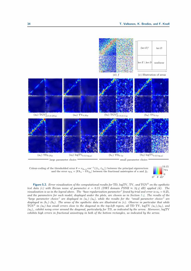
34 T. Valkonen, K. Bredies, and F. Knoll
(d) f
kerE \ kerD
(kerE)c kerD
nonlinear
(e) Illustration of areas
(a3) TGV2(2.5,0.25)µ (a4) TV0.25µ (b3) TGV2
(0.15,0.1)µ (b4) TV0.1µ
(a1) TD0.25µ (a2) logTV0.5| log µ| (b1) TD0.1µ (b2) logTV0.2| log µ|
large parameter choice small parameter choice
0
eFA
0.15
0 θ 45
Colour-coding of the thresholded error θ = νf0,u cos−1(〈vu, vf0 〉) between the principal eigenvectorsand the error eFA = |FAu − FAf0 | between the fractional anistropies of u and f0.
Figure 5.2. Error visualisation of the computational results for TD, logTV, TV, and TGV2 on the synthetictest data (c) with Rician noise of parameter σ = 0.15 (DWI domain PSNR ≈ 34.4 dB) applied (d). Thevisualisation is as in the legend above. The “base regularisation parameter” found by trial and error is α0 = 0.25,and the parameters for each model, displayed under the plots, are chosen as in Section 5.4. The results of the“large parameter choice” are displayed in (a1)–(a4), while the results for the “small parameter choice” aredisplayed in (b1)–(b4). The areas of the synthetic data are illustrated in (e). Observe in particular that whileTGV2 in (a3) has small errors close to the diagonal in the top-left region, all TD TV, logTV (a1),(a2), and(a4),, exhibit noisy error around the diagonal, particularly for TD, as indicated by the arrow. Moreover, logTVexhibits high errors in fractional anisotropy in both of the bottom rectangles, as indicated by the arrow.

Total generalised variation in DTI 35
(c) f0 (a5) DWITV9.8
iter 80dF 15.69µdA 64.28dv 58.67dλ 10.85µ
iter 80dF 15.69µdA 64.28dv 58.67dλ 10.85µ
(d) f
dF 24.33µdA 75.10dv 62.49dλ 13.25µ
dF 24.33µdA 75.10dv 62.49dλ 13.25µ
(b5) DWITV3.9
iter 80dF 15.55µdA 74.26dv 60.89dλ 10.10µ
iter 80dF 15.55µdA 74.26dv 60.89dλ 10.10µ
(a3) TGV2(0.5,0.05)µ
iter 2841dF 16.25µdA 68.91dv 61.69dλ 10.22µ
iter 2841dF 16.25µdA 68.91dv 61.69dλ 10.22µ
(a4) TV0.05µ
iter 74dF 15.90µdA 66.60dv 61.00dλ 10.00µ
iter 74dF 15.90µdA 66.60dv 61.00dλ 10.00µ
(b3) TGV2(0.03,0.02)µ
iter 155dF 17.50µdA 70.51dv 60.49dλ 11.36µ
iter 155dF 17.50µdA 70.51dv 60.49dλ 11.36µ
(b4) TV0.02µ
iter 77dF 17.11µdA 69.99dv 60.23dλ 10.97µ
iter 77dF 17.11µdA 69.99dv 60.23dλ 10.97µ
(a1) TD0.05µ
iter 75dF 16.37µdA 68.82dv 61.61dλ 10.30µ
iter 75dF 16.37µdA 68.82dv 61.61dλ 10.30µ
(a2) logTV0.05| log µ|
iter 80dF 19.37µdA 71.62dv 62.52dλ 12.84µ
iter 80dF 19.37µdA 71.62dv 62.52dλ 12.84µ
(b1) TD0.02µ
iter 78dF 17.51µdA 70.43dv 60.44dλ 11.33µ
iter 78dF 17.51µdA 70.43dv 60.44dλ 11.33µ
(b2) logTV0.02| log µ|
iter 80dF 20.93µdA 71.61dv 62.13dλ 14.50µ
iter 80dF 20.93µdA 71.61dv 62.13dλ 14.50µ
large parameter choice small parameter choice
xy
zColour-coding vu ·min1, FAu + 1/3 of the principal eigenvectorvu modulated by the fractional anisotropy FAu
Figure 5.3. Computational results for TD, logTV, TV, TGV2, and DWITV on the in-vivo brain data(c) with Rician noise of parameter σ = 10 (DWI domain PSNR ≈ 29.0 dB) applied (d). The visualisationis as in the legend above. The “base regularisation parameter” found by trial and error is α0 = 0.05, and theparameters for each model, displayed under the plots, are chosen as in Section 5.4. The results of the “largeparameter choice” are displayed in (a1)–(a4), while the results for the “small parameter choice” are displayed in(b1)–(b4). The iteration counts and error measures discussed in Subsection 5.1 have been superimposed on theresults. Observe in particular the stair-casing of TV and logTV particularly in the green region on lower-leftindicated by the arrow in the logTV plot.

36 T. Valkonen, K. Bredies, and F. Knoll
(a5) DWITV9.8 (d) f (b5) DWITV3.9
(a3) TGV2(0.5,0.05)µ (a4) TV0.05µ (b3) TGV2
(0.03,0.02)µ (b4) TV0.02µ
(a1) TD0.05µ (a2) logTV0.05| log µ| (b1) TD0.02µ (b2) logTV0.02| log µ|
large parameter choice small parameter choice
0
eFA
0.15
0 θ 45
Colour-coding of the thresholded error θ = νf0,u cos−1(〈vu, vf0 〉) between the principal eigenvectorsand the error eFA = |FAu − FAf0 | between the fractional anistropies of u and f0.
Figure 5.4. Error visualisation of the computational results for TD, logTV, TV, TGV2, and DWITV onthe in-vivo brain data (c) with Rician noise of parameter σ = 10 (DWI domain PSNR ≈ 29.0 dB) applied (d).The visualisation is as in the legend above. The “base regularisation parameter” found by trial and error isα0 = 0.05, and the parameters for each model, displayed under the plots, are chosen as in Section 5.4. Theresults of the “large parameter choice” are displayed in (a1)–(a4), while the results for the “small parameterchoice” are displayed in (b1)–(b4). Observe in particular how TGV2 (and TD) restore the fractional anisotropybetter than TV (or logTV), with less intense white areas, as indicated by the arrows.

Total generalised variation in DTI 37
(c) f0 (a5) DWITV31
iter 78dF 23.98µdA 77.80dv 65.97dλ 16.22µ
iter 78dF 23.98µdA 77.80dv 65.97dλ 16.22µ
(d) f
dF 31.72µdA 80.00dv 69.35dλ 16.43µ
dF 31.72µdA 80.00dv 69.35dλ 16.43µ
(b5) DWITV13
iter 79dF 24.52µdA 78.05dv 67.68dλ 14.85µ
iter 79dF 24.52µdA 78.05dv 67.68dλ 14.85µ
(a3) TGV2(1.5,0.15)µ
iter 552dF 22.99µdA 63.69dv 68.76dλ 14.95µ
iter 552dF 22.99µdA 63.69dv 68.76dλ 14.95µ
(a4) TV0.15µ
iter 70dF 23.80µdA 58.30dv 65.85dλ 15.94µ
iter 70dF 23.80µdA 58.30dv 65.85dλ 15.94µ
(b3) TGV2(0.09,0.06)µ
iter 867dF 22.92µdA 72.16dv 67.70dλ 14.10µ
iter 867dF 22.92µdA 72.16dv 67.70dλ 14.10µ
(b4) TV0.06µ
iter 70dF 22.88µdA 68.82dv 66.25dλ 14.40µ
iter 70dF 22.88µdA 68.82dv 66.25dλ 14.40µ
(a1) TD0.15µ
iter 68dF 23.25µdA 63.61dv 68.83dλ 15.13µ
iter 68dF 23.25µdA 63.61dv 68.83dλ 15.13µ
(a2) logTV0.15| log µ|
iter 79dF 23.82µdA 76.29dv 66.89dλ 14.76µ
iter 79dF 23.82µdA 76.29dv 66.89dλ 14.76µ
(b1) TD0.06µ
iter 72dF 23.15µdA 71.81dv 67.58dλ 14.25µ
iter 72dF 23.15µdA 71.81dv 67.58dλ 14.25µ
(b2) logTV0.06| log µ|
iter 80dF 24.01µdA 75.65dv 67.37dλ 15.07µ
iter 80dF 24.01µdA 75.65dv 67.37dλ 15.07µ
large parameter choice small parameter choice
xy
zColour-coding vu ·min1, FAu + 1/3 of the principal eigenvectorvu modulated by the fractional anisotropy FAu
Figure 5.5. Computational results for TD, logTV, TV, TGV2, and DWITV on the in-vivo brain data(c) with Rician noise of parameter σ = 50 (DWI domain PSNR ≈ 14.5 dB) applied (d). The visualisationis as in the legend above. The “base regularisation parameter” found by trial and error is α0 = 0.15, and theparameters for each model, displayed under the plots, are chosen as in Section 5.4. The results of the “largeparameter choice” are displayed in (a1)–(a4), while the results for the “small parameter choice” are displayedin (b1)–(b4). The iteration counts and error measures discussed in Subsection 5.1 have been superimposed onthe results. The rectangle in (c) indicates the corpus callosum displayed in more detail in Figure 5.7. Observein particular the small extremely bright spots (high fractional anisotropy) exhibited by logTV, indicated by thearrow, and the extreme stair-casing of TV for the large parameter choice. At the same time, TGV2 and TDperform reasonably well for the large parameter choice, while all methods leave significant amounts of noise forthe small parameter choice. And, yet, logTV exhibits stair-casing already for the small parameter choice, asindicated by an arrow.

38 T. Valkonen, K. Bredies, and F. Knoll
(a5) DWITV31 (d) f (b5) DWITV13
(a3) TGV2(1.5,0.15)µ (a4) TV0.15µ (b3) TGV2
(0.09,0.06)µ (b4) TV0.06µ
(a1) TD0.15µ (a2) logTV0.15| log µ| (b1) TD0.06µ (b2) logTV0.06| log µ|
large parameter choice small parameter choice
0
eFA
0.15
0 θ 45
Colour-coding of the thresholded error θ = νf0,u cos−1(〈vu, vf0 〉) between the principal eigenvectorsand the error eFA = |FAu − FAf0 | between the fractional anistropies of u and f0.
Figure 5.6. Error visualisation of the computational results for TD, logTV, TV, TGV2, and DWITV onthe in-vivo brain data (c) with Rician noise of parameter σ = 50 (DWI domain PSNR ≈ 14.5 dB) applied (d).The visualisation is as in the legend above. The “base regularisation parameter” found by trial and error isα0 = 0.15, and the parameters for each model, displayed under the plots, are chosen as in Section 5.4. Theresults of the “large parameter choice” are displayed in (a1)–(a4), while the results for the “small parameterchoice” are displayed in (b1)–(b4). Observe the high errors of fractional anisotropy exhibited by TV, as indicatedby the arrow.

Total generalised variation in DTI 39
(c) f0 (a5) DWITV31 (d) f (b5) DWITV13
(a3) TGV2(1.5,0.15)µ (a4) TV0.15µ (b3) TGV2
(0.09,0.06)µ (b4) TV0.06µ
(a1) TD0.15µ (a2) logTV0.15| log µ| (b1) TD0.06µ (b2) logTV0.06| log µ|
large parameter choice small parameter choice
0 FA 1
Greyscale-coding of thefractional anisotropy
Figure 5.7. Fractional anisotropy (see legend above) and planar projection of the principal eigenvector forthe region containing the corpus callosum of the in-vivo brain data (c). Rician noise of parameter σ = 50 (DWIdomain PSNR ≈ 14.5 dB) has been applied to yield the noisy data (d). The “base regularisation parameter”found by trial and error is α0 = 0.15, and the parameters for each model, displayed under the plots, are chosenas in Section 5.4. Denoising results of the the noisy data for the “large parameter choice” with for TD, logTV,TV, TGV2, and DWITV are displayed in (a1)–(a5), while the denoising results for the “small parameter choice”are displayed in (b1)–(b5). Observe the noisy reconstruction of fractional anisotropy by logTV, as indicated bythe arrow.