tools for atmospheric radiative transfer: streamer and fluxnet

TOOLS FOR ATMOSPHERIC RADIATIVE TRANSFER:

STREAMER AND FLUXNET

JEFFREY R. KEY1 and AXEL J. SCHWEIGER2

1Department of Geography, Boston University, 675 Commonwealth Ave., Boston, MA 02215, U.S.A.,and 2Polar Science Center, University of Washington, Seattle, WA, U.S.A.

(e-mail: [email protected])

(Received 12 June 1997; revised 9 October 1997)

AbstractÐTwo tools for the solution of radiative transfer problems are presented. Streamer is a ¯exiblemedium spectral resolution radiative transfer model based on the plane-parallel theory of radiativetransfer. Capable of computing either ¯uxes or radiances, it is suitable for studying radiative processesat the surface or within the atmosphere and for the development of remote-sensing algorithms. FluxNetis a fast neural network-based implementation of Streamer for computing surface ¯uxes. It allows for asophisticated treatment of radiative processes in the analysis of large data sets and potential integrationinto geophysical models where computational e�ciency is an issue. Documentation and tools for thedevelopment of alternative versions of FluxNet are available. Collectively, Streamer and FluxNet solvea wide variety of problems related to radiative transfer: Streamer provides the detail and sophisticationneeded to perform basic research on most aspects of complex radiative processes, whereas the e�ciencyand simplicity of FluxNet make it ideal for operational use. # 1998 Elsevier Science Ltd. All rightsreserved

Code available at http://www.iamg.org/CGEditor/index.htm

Key Words: Radiative transfer models, Atmospheric processes, Radiation budget, Satellites.

INTRODUCTION

The transfer of solar (shortwave) and terrestrial

(longwave) radiation through the atmosphere in¯u-

ences all aspects of the climate system. For a signi®-

cant portion of the earth's surface the radiation

budget is the dominant term in the surface energy

balance. Understanding how radiation is attenuated

by clouds, aerosols, and gases as it passes through

the atmosphere is therefore a prerequisite to under-

standing the dynamic and thermodynamic com-

ponents of the global climate system. For example,

the radiative e�ect of clouds in¯uences heating and

cooling within the atmosphere, which in turn in¯u-

ence the vertical and horizontal movement of air.

But the cloud radiative e�ect is not the same for all

clouds, and depends upon the cloud thickness, par-

ticle size distribution, density, and vertical position.

Gases also play an important role in radiative

transfer. Indeed, the ``greenhouse e�ect'', as applied

to the earth's atmosphere, is a radiative process

summarizing the absorption and emission of terres-

trial radiation by gases such as carbon dioxide,

water vapor, and methane.

In this paper two general purpose tools for sol-

ving atmospheric radiative transfer problems are

described. The ®rst, Streamer, is a medium spectral

resolution model suitable for studying the radiation

budgets at the surface and within the atmosphere.

It can also be used to simulate satellite sensor ob-

servations. The second tool, FluxNet, is a neural

network-based radiative transfer model trained on

Streamer calculations, but is limited to the calcu-

lation of radiative ¯uxes at the surface. Its advan-

tage is that it is extremely fast. This is important

for processing large data sets or including sophisti-

cated radiative transfer calculations in complex geo-

physical models. Each of these tools is designed to

provide solutions to a wide array of radiative trans-

fer problems.

A variety of other radiative transfer models exist,

both for the calculation of radiative ¯uxes and the

simulation of radiances measured by satellite sen-

sors. However, those used for the calculation of

radiative ¯uxes are generally components of climate

models (cf. Ellingson, Ellis and Fels, 1991) and are

not well documented or easy to use. For this reason

they will not be discussed further in this paper.

Radiative transfer models that are well documented,

reliable, and available to the scienti®c community

include LOWTRAN (Kneizys and others, 1988),

MODTRAN (Snell and others, 1995), and 6S

(Vermote and others, 1994). Although there are

others, these three have been widely used in remote

sensing applications. They are all medium or high

spectral resolution band models and incorporate

thorough treatments of gas absorption (Table 1).

However, the cloud models in LOWTRAN/

Computers & Geosciences Vol. 24, No. 5, pp. 443±451, 1998# 1998 Elsevier Science Ltd. All rights reserved

Printed in Great Britain0098-3004/98 $19.00+0.00PII: S0098-3004(97)00130-1

443

MODTRAN are not easily modi®ed, and the two-stream approximation for multiple scattering results

in signi®cant errors under certain conditions.Additionally, none of these models computes ¯uxesdirectly, and the user interfaces for LOWTRAN

and MODTRAN are somewhat crude. The 6Smodel is commonly used for atmospheric correc-tions, but it is limited to the shortwave and does

not include clouds.Streamer and FluxNet were developed to address

some of these shortcomings for applications invol-

ving the assimilation of satellite-derived informationinto atmosphere±ice±ocean models. Requirementsincluded the ability to simulate satellite radiancesfor algorithm development, incorporate a sophisti-

cated treatment of radiative processes in a coupledice±ocean model, and generate large satellite-de-rived forcing ®elds. A ¯exible interface to specify

cloud and surface optical properties not commonlyfound in other radiative transfer models was im-portant in the development of these two tools.

Although both have their origin in polar research,they have been extended and applied to global pro-blems.

STREAMER

Streamer is a general purpose atmospheric radia-tive transfer model that computes either radiances(intensities) or irradiances (¯uxes) for a wide variety

of atmospheric and surface conditions. Its userinterface is extremely ¯exible and easy to use.Streamer's major features are:(1) Radiances for any polar and azimuthal angles,

shortwave and longwave ¯uxes, net ¯uxes, cloudradiative e�ect (``cloud forcing''), and heating ratescan be computed at any atmospheric level.

(2) Both two-stream and discrete ordinates sol-vers are included.(3) Gas absorption and clouds are parameterized

for 24 shortwave and 105 longwave bands.(4) Built-in atmospheric data include water and

ice cloud optical properties, ®ve aerosol opticalmodels, four aerosol vertical pro®les, and seven

standard atmospheric pro®les. Either standard oruser-de®ned pro®les can be used, or total columnamounts of water vapor, ozone, and aerosols can

be speci®ed.(5) Each computation is done for a ``scene'',

where the scene can be a mixture of up to 10 cloud

types occurring individually, up to 10 overlappingcloud sets of up to 10 clouds each, and clear sky,all over some combination of up to three surface

types.(6) Spectral albedo data for open ocean (sea

water), meltponds, bare ice, snow, green vegetation,and dry sand are included.

(7) The user interface provides looping structuresfor up to ten variables at a time; variables can be

reassigned, and output can be easily customized.Processing is controlled by a set of options and

input data. The options de®ne the characteristics

common to all the data, while the data provides in-formation for each scene or case (e.g. a pixel or ob-servation in time). Output includes surface and top

of the atmosphere (TOA) radiative ¯uxes, surfacealbedo, and cloud radiative e�ect for ¯ux calcu-lations, or radiances and TOA albedo or brightness

temperature. Either of two ®les may be written: onewith labeled results or one that is user-customiz-able.

Components

Two radiative transfer solvers are used in

Streamer: a two-stream method and a discrete ordi-nate solver. The discrete ordinate radiative transfer(DISORT) solver is described in Stamnes and

others (1988) and has been available to the publicas a stand-alone package for many years. The two-stream method is described in Toon, McKay andAckerman (1989). It uses a Delta±Eddington ap-

proximation for the shortwave and a hemisphericmeans approximation for the longwave portion ofthe spectrum. The discrete ordinate solver is the

more accurate of two, and can be used to computeeither radiances or ¯uxes. The two-stream solvercomputes only ¯uxes but is much faster than

DISORT. Di�erences in ¯uxes computed using thetwo methods are generally small, but can be signi®-cant under certain circumstances. For example,

two-stream results for longwave ¯uxes are within0.5 W mÿ2 of the 24-stream discrete ordinatesvalues. In the shortwave, di�erences depend on thesurface albedo and the illumination geometry. The

two- and 24-stream ¯uxes are within about 1% fora dark surface and a high sun, but at the otherextreme, di�erences are as high as 10% with a large

solar zenith angle and/or a bright surface.Cloud optical properties are based on parameteri-

zation schemes from three di�erent sources. For

water clouds, the data are taken from Hu andStamnes (1993). E�ective radii, the ratio of thethird to the second moments of the particle size dis-tribution, range from 2.5 to 60 mm and are given

for 293 wavelengths throughout the shortwave andlongwave portions of the spectrum. For ice cloudsin the shortwave, the ®ve-band parameterization of

Ebert and Curry (1992), based on randomlyoriented hexagonal cylinders, is used. Longwave icecloud optical properties are based on Mie calcu-

lations using spherical particles for 132 wavelengths.This parameterization is unpublished but followsthe methodology of Hu and Stamnes. Of course,

using spherical particles in the determination of icecloud optical properties may not be realistic, sinceice crystals may take on a variety of shapes (cf.,Takano and Liou, 1989; Schmidt and others, 1995).

J. R. Key and A. J. Schweiger444

However, no parameterization using other shapes(e.g. hexagons) across the entire longwave range is

currently available. Both the water and ice cloud

parameterizations of optical properties are based on

the empirical relationship between the particle e�ec-

tive radius and extinction, single scatter albedo, theasymmetry parameter, and the cloud water content.

For radiative transfer calculations, water cloud and

longwave ice cloud optical properties are averaged

over Streamer spectral bands.

Aerosol amounts as extinction coe�cients can be

distributed vertically according to a user-supplied

pro®le or one of the internal standard pro®les.

Four vertical pro®le shapes are available that arecombinations of two tropospheric and two strato-

spheric loadings, based on data in the LOWTRAN-

7 radiative transfer model (Kneizys and others,

1988). Tropospheric background, rural, urban, mar-

itime (Shettle and Fenn, 1979) and Arctic haze

(Blanchet and List, 1983) aerosol optical propertymodels are available. Standard temperature and

humidity pro®les include tropical, mid-latitude, sub-

arctic, and arctic. They are based on data in

Ellingson, Ellis and Fels, (1991) except for the

Arctic pro®les of temperature and humidity, whichare derived from Arctic Ocean coastal and drifting

station data. Gaseous absorption is parameterizedusing an exponential sum ®tting technique

(Wiscombe and Evans, 1977) with coe�cients pro-

vided by S.-C. Tsay (personal communication,

1991; cf., Tsay, Stamnes and Jayaweera, 1989).

Only four gases are present in Streamer: watervapor, carbon dioxide, ozone, and oxygen.

Several spectral albedo data sets are available inStreamer. Sand and vegetation data are from

Vermote and others (1994); meltpond and bare ice

albedos are from Grenfell and Maykut (1977); sea

water data are based on Brieglieb and others

(1986); freshwater albedos are from Fresnel calcu-lations; and snow spectral albedos were computed

using a four-stream model based on the ideas of

Warren and Wiscombe (1980). Surface bi-direc-

tional re¯ectance functions can not currently be

employed.

Streamer includes band weights to approximate

the sensor spectral response functions of theAdvanced Very High Resolution Radiometer

(AVHRR) on-board the NOAA polar orbiting sat-

ellites, the Along Track Scanning Radiometer

(ATSR) on ERS-1, the High Resolution Infrared

Radiation Sounder (HIRS/2) of the TirosOperational Vertical Sounder (TOVS) on NOAA

Table 1. Comparison of selected features of popular radiative transfer models

LOWTRAN MODTRAN 6S Streamer

Numericalapproximationmethod

Two-stream, includingatmospheric refraction

Two-stream, includingatmosphericrefraction; discreteordinates also inMODTRAN-3

Successive orders ofscattering

Discrete ordinates andtwo-stream

Spectral resolution 20 cmÿ1 2 cmÿ1 10 cmÿ1, shortwaveonly

24 shortwave bands;20 cmÿ1 bandwidth inlongwave

Clouds Eight cloud models Eight cloud models No clouds Flexible speci®cationof cloud optical andphysical properties

Aerosols Four optical models Four optical models Six optical models Five optical models

Gas absorption* Principle and tracegases

Principle and tracegases

Principle and tracegases

Principle gases only

Atmospheric pro®les Standard and user-speci®ed

Standard and user-speci®ed

Standard and user-speci®ed

Standard plus Arcticand user-speci®ed

Surface characteristics Lambertian, no built-in models

Lambertian, no built-in models

Lambertian spectralalbedo models built-in; Bi-directionallyre¯ecting surfacepossible

Lambertian, built-inspectral albedomodels

Primary outputparameter

Radiance Radiance Radiance/re¯ectance Radiance/re¯ectance/brightnesstemperature or ¯ux

User interface Formatted input ®le Formatted input ®le Input ®le Input ®le withcommand language

*In this table, principal gases are H2O, O3, CO2, and O2. Trace gases include, among others, CH4, N2O, and CO.

Tools for atmospheric radiative transfer 445

polar orbiters, and the Moderate ResolutionImaging Spectroradiometer (MODIS), a future

NASA instrument. However, with only 24 short-wave bands and longwave bands of 20 cmÿ1 width,satellite applications are limited to the broader

band sensors. For example, the longwave channelsof the AVHRR and the ATSR span as many as sixStreamer spectral bands but the shortwave channels

cover as few as one. There are a few HIRS andMODIS channel pairs that are completely con-tained within the same Streamer spectral band, so

no distinction between them is possible. For othersensors, the user can specify band weights and cen-tral wavenumbers.

Running Streamer

Streamer can be run in two modes. The stand-

alone mode allows the solution of radiative transferproblems with input and output speci®ed from oneor more ®les. This mode is ideal for asking ques-

tions related to radiative transfer such as satellitealgorithm development or sensitivity studies. In thesecond, Streamer is called as a Fortran subroutine.

This mode allows Streamer to be integrated intomodels or data processing systems.To run Streamer as a stand-alone model a ®le

containing a sequence of commands and data is

used. The command set includes: $OPTIONS,$SETDATA, $CASE, $REPLACE, $EXCHANGE,$PRINT, and $COMMENT. The $OPTIONS com-

mand indicates that a block of options containingvariables common to all cases (or ``scenes'') shouldbe read. The $SETDATA and $CASE commands

signify that data for a new case are to be read. The$REPLACE and $EXCHANGE commands areused to assign or reassign variable values from the

previous scene's data, and can be used to initiateloops. Speci®c variables can be printed for each

case without having to modify the source code by

using $PRINT. Comments can be added to the

input ®le with $COMMENT or simply with ``;''.

The input data types are ¯exible (Table 2). For

example, if the solar zenith angle is not speci®ed

then it will be computed; the surface albedo speci®-

cation can be broadband, visible band, or multi-

band; cloud thickness can be speci®ed as optical

thickness, thickness in pressure or height units;

water vapor, aerosol, and ozone pro®les can be pro-

vided or total column amounts can be speci®ed.

When less detail than needed is provided, built-in

data are used.

With $REPLACE and $EXCHANGE scalar

variables can be assigned new values, as can indi-

vidual array elements or entire arrays. These com-

mands also provide the facility for doing

calculations over a range of variable values. Two

looping structures are available, one where the

starting, ending, and increment values are speci®ed

as in most high-level programming languages, and

another where all values to be evaluated are speci-

®ed. If more than one loop is speci®ed, they are

nested. As an example, the following statement

reassigns the solar zenith angle and loops over a

range of cloud particle e�ective radii from 2 to

10 mm in increments of 1 mm, and loops over a list

of ®ve cloud optical thicknesses for each e�ective

radius.

$replace zen = 65.0;cldre(1) = (2, 10., 1.);cldthick(1) = [0,1, 2, 4, 8]

Default output includes descriptive text and

values for surface and top of the atmosphere radia-

tive ¯uxes, surface albedo, and cloud radiative e�ect

for ¯ux calculations, or radiances and TOA albedo

or brightness temperatures (Table 3). The $PRINT

Table 2. Streamer input options and data descriptions (not comprehensive)

Category Variable Type

Options Fluxes or radiances?Number of streams, shortwave and longwaveGaseous absorption?Rayleigh scattering?Surface albedo and emissivity typeStandard temperature and humidity pro®le typeAerosol pro®le shape and optical modelUnits selectionBand weight ®le nameOutput ®le name

Location, viewing geometry, bands Year, month, day, hour, latitude, longitude or solar zenith angle. Viewingangles. Starting and ending spectral bands or channel

Surface Albedo, surface types and fractionsCharacteristics Temperature and emissivity

Cloud Optical or physical thickness, top or bottom temperatureCharacteristics Height, particle e�ective radius, phase, fraction. Overlapping sets

Pro®les Pro®le input options, pro®les or column amounts


command can be used to select only those par-

ameter values of interest with or without the

descriptive text. For example, the following state-

ment prints some descriptive text and just a few

variable values on two separate lines:

$print 'bstart, bend:',bstart, bend,/NEWLINE,

'Re, albedo, zenith angle:', cldre, satalb(1,2), zen

This statement is speci®ed once but will be

applied to every case in the input ®le.

While the user interface with $REPLACE and

$PRINT provides tremendous ¯exibility and con-

trol, there may be applications where Streamer

needs to be integrated into existing Fortran code.

For example, simple parameterizations of radiative

¯uxes currently used in sea ice models could be

replaced with a radiative transfer model. In appli-

cations such as this, Streamer is available as a sub-

routine, where all basic data normally given in the

input ®le are passed in as a list of arguments to the

subroutine. Output data are passed back to the call-

ing routine.

Table 3. Output variable types available in Streamer

Category Variable type

Header Information Repeat of input options

Pro®les Height, pressure, temperature, water vapor density, relative humidity, ozone,and aerosol extinction, total column amounts

Cloud Characteristics Physical thickness, pressure thickness, optical thickness, fraction, toptemperature, top pressure and height, e�ective radius, liquid/ice water content,phase, overlap sets

Surface Characteristics Clear sky fraction, fraction of each surface type, input surface albedo at 0.6 mm,surface temperature, broadband surface albedo

Fluxes Downwelling direct, di�use, and total shortwave, downwelling longwave,upwelling shortwave and longwave, net irradiances, heating/cooling rates, cloudradiative e�ect

Radiances Spectrally integrated for each polar angle, azimuthal angle, and level; top levelalbedo and/or brightness temperature

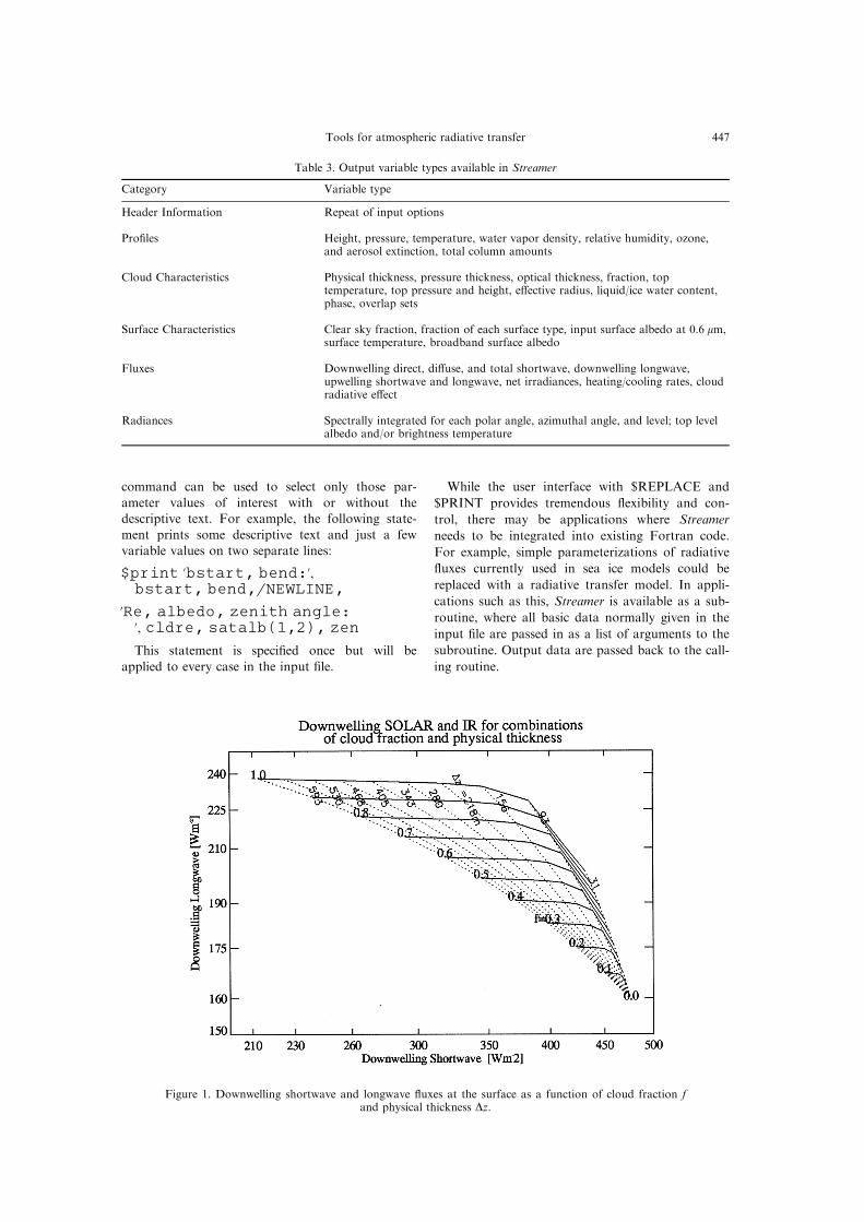
Figure 1. Downwelling shortwave and longwave ¯uxes at the surface as a function of cloud fraction fand physical thickness Dz.


Figure 2. Brightness temperatures and temperature di�erences in two infrared window channels as afunction of cloud optical depth t and droplet e�ective radius Re.

Figure 3. Downwelling longwave ¯uxes (W mÿ2) at the surface computed using TOVS-derived pro®lesand cloud properties. (Courtesy of J. Francis).


Sample applications

Figures 1±3 provide a few examples of how

Streamer has been used. Figure 1 gives downwelling

shortwave and longwave ¯uxes as a function ofcloud physical thickness and cloud fractional cover-

age in the scene. These data were generated using

the looping structures in the $REPLACE com-

mand. Figure 2 shows top of the atmospherebrightness temperatures and brightness temperature

di�erences for the 11 and 12 mm channels of the

AVHRR over a range of cloud optical depths and

droplet e�ective radii for a speci®c set of viewing,atmospheric, and surface conditions. This type of

data can be used for the retrieval of cloud e�ective

radius and optical depth from AVHRR obser-

vations. Figure 3 shows downwelling longwave¯uxes over the Arctic that were computed using

cloud and atmospheric parameters derived from the

TOVS.

FLUXNET

FluxNet is an arti®cial neural network implemen-

tation of the two-stream radiative transfer solution

for surface ¯uxes in Streamer. Arti®cial neural net-

works have been applied to tasks involving the

analysis of complex patterns such as signal proces-

sing, optical character recognition, and even stock

market forecasting. Although a variety of architec-

tures have been created, the three- and four-layer

backpropagation networks are the most popular.

The signals from the input units are fed forward

through processing nodes in the hidden layers to

the output units. The output is then compared to

desired results, the error is propagated backwards

from the output layer through the hidden layers,

and the weight of each connection is adjusted

accordingly. Characteristics of neural networks that

make them attractive are: (1) the four-layer network

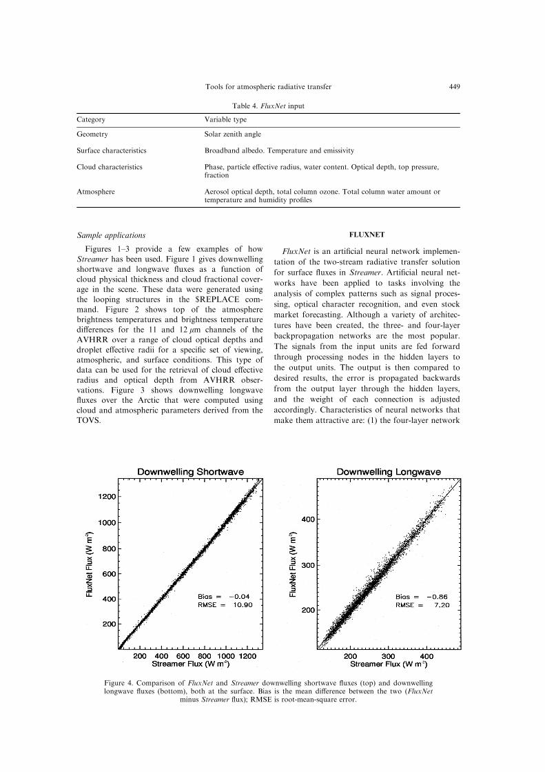
Figure 4. Comparison of FluxNet and Streamer downwelling shortwave ¯uxes (top) and downwellinglongwave ¯uxes (bottom), both at the surface. Bias is the mean di�erence between the two (FluxNet

minus Streamer ¯ux); RMSE is root-mean-square error.

Table 4. FluxNet input

Category Variable type

Geometry Solar zenith angle

Surface characteristics Broadband albedo. Temperature and emissivity

Cloud characteristics Phase, particle e�ective radius, water content. Optical depth, top pressure,fraction

Atmosphere Aerosol optical depth, total column ozone. Total column water amount ortemperature and humidity pro®les


can, theoretically, determine any computable func-tion, (2) no assumptions about the statistical distri-

bution of input variables are made, and (3) they arefast once they are trained. However, since neuralnetwork-based estimation methods do not include

any assumptions about the underlying non-linearphysics, estimates can only be truly optimal withrespect to the training data set and estimation

errors need to be determined through the appli-cation to an independent test or validation data set.FluxNet was trained with surface radiative ¯uxes

computed by Streamer. Ten thousand cases encom-passing a wide range of global surface and atmos-pheric conditions were used in the training. Thefour outputs are downwelling and upwelling, short-

wave and longwave ¯uxes at the surface. The inputvariables to FluxNet constitute a subset of thoserequired for Streamer, as listed in Table 4. Two ver-

sions of the network are currently available: onerequiring temperature and humidity pro®les in theinput stream and one using the total column water

vapor rather than the pro®les. The code is shortand fast. C and IDL (Interactive Data Languagefrom Research Systems, Boulder) programming

language versions are available. Detailed instruc-tions and tools for creating custom networks aregiven in the software documentation.FluxNet is a simpler model than Streamer. Its

principal advantage is that it is faster by two tofour orders of magnitude (100 to 10 000 times),making it ideal for large jobs like image processing,

which consist of thousands to millions of di�erentcases. Users of Streamer should be aware of the fol-lowing limitations in FluxNet:

(1) Each scene can consist of just one surfacetype and one cloud layer.(2) The 24 shortwave and 105 longwave spectral

bands in Streamer have been consolidated into one

shortwave and one longwave band; i.e. only broad-band calculations are done.(3) Input and output data types, ordering, and

units are ®xed, there are no options and no com-mand language.A comparison between FluxNet and Streamer

downwelling ¯uxes for 5000 test cases is shown inFigure 4. The biases (mean di�erences) are close tozero, and the root-mean-square errors are 2±3% of

the mean ¯ux values. Additionally, 90% of theerrors are 5% or less, which is within the accuracy(3±5%) of radiometers frequently used in the ®eld.However, for shortwave ¯uxes less than about

20 W mÿ2 errors can be up to 30%. Upwelling¯uxes (not shown) have smaller root-mean-squareerrors.

SUMMARY

Streamer and FluxNet are tools for the solutionof a wide variety of radiative transfer problems.

Streamer is a ¯exible and customizable general-pur-pose radiative-transfer model. It allows for the com-

putation of both irradiances and radiances and istherefore suitable for the simulation of some satel-lite signals and the study of radiative heat budgets

in the atmosphere or at the surface. Weighing func-tions for a number of satellite sensors are provided.Users can select from a wide range of built-in at-

mospheric pro®les and surface types. Speci®cationof cloud properties is in terms of e�ective particlesize, water content, physical or optical thickness,

and vertical position. Streamer can be run in astand-alone mode or called as a subroutine.FluxNet provides a computationally e�cientmethod for a sophisticated treatment of radiative

transfer processes and is therefore suitable for theprocessing of large data sets or incorporation withinmodels. FluxNet is 100 to 10 000 times faster than

Streamer. For instantaneous observations, di�er-ences (root-mean-square errors) between Streamerand FluxNet are on the order of 11 W mÿ2 for

downwelling shortwave ¯uxes and 7 W mÿ2 fordownwelling longwave ¯uxes without signi®cantbiases. Assuming daily sampling for monthly aver-

age calculations these errors are reduced by a factorof ®ve (square root of 30; cf. Key et al., 1997),which is well within the requirements of 10 W mÿ2

for monthly surface ¯uxes (WMO, 1987).

Streamer is implemented in Fortran 77 and hasbeen compiled and tested on Intel, Sun, SGI, HP,IBM, and DEC platforms. Ports to other platforms

should be straightforward. FluxNet is available inANSI C and IDL (Interactive Data Language) andhas been tested on Intel and Sun platforms.

Detailed instructions for creating custom networksare given in the documentation. Streamer andFluxNet may be obtained by anonymous ftp fromstratus.bu.edu (or iamg.org) or through the World

Wide Web at http://stratus.bu.edu. Source code,user guides, and test input/output data are pro-vided.

AcknowledgmentsÐStreamer has its roots in the programstrats by S.-C. Tsay. Much of the strats code was used inthe original version of Streamer (ca. 1992) and some com-ponents remain an integral part of the model. The two-stream solution is based on code from T. Ackerman.Thanks to R. Stone for many valuable discussions and forassistance in the ice cloud Mie calculations. The StuttgartNeural Network Simulator by Andreas Zell and others(http://www.informatik.uni-stuttgart.de/ipvr/bv/projekte/s-nns/snns.html) was used in the development of FluxNet.Funding was provided primarily by the NASA EOS inter-disciplinary project POLES (NAGW-2407) and by NASAPolar Programs grants NAGW-4169 and NAGW-3437.

REFERENCES

Blanchet, J.-P. and List, R. (1983) Estimation of opticalproperties of Arctic haze using a numerical model.Atmosphere-Ocean 21(4), 444±465.

Brieglieb, B. P., Minnis, P., Ramanathan, V. andHarrison, E. (1986) Comparison of regional clear-sky


albedos inferred from satellite observations and modelcomputations. Journal of Climate and AppliedMeteorology 25, 214±226.

Ebert, E. E. and Curry, J. A. (1992) A parameterizationof ice cloud optical properties for climate models.Journal of Geophysical Research 97(D4), 3831±3836.

Ellingson, R. G., Ellis, J. and Fels, S. (1991) The inter-comparison of radiation codes used in climate models:long wave results. Journal of Geophysical Research96(D5), 8929±8953.

Grenfell, T. C. and Maykut, G. A. (1977) The opticalproperties of ice and snow in the arctic basin. Journalof Glaciology 18(80), 445±463.

Hu, Y. X. and Stamnes, K. (1993) An accurate parameter-ization of the radiative properties of water clouds suit-able for use in climate model. Journal of Climate 6(4),728±742.

Key, J., Schweiger, A. J. and Stone, R. S. (1997) Expecteduncertainty in satellite-derived estimates of the high-latitude surface radiation budget. Journal ofGeophysical Research, in press.

Kneizys, F. X., Shettle, E. P., Abreu, L. W., Chetwynd, J.H, Anderson, G. P., Gallery, W. O., Selby, J. E. A.and Clough, S. A. (1988) Users Guide toLOWTRAN7. Environmental Research Papers, No.1010, AFGL-TR-88-0177, Air Force GeophysicsLaboratory, Hanscom AFB, Massachusetts, 137 pp.

Schmidt, E. O., Arduini, R. F., Wielicki, B. A., Stone,R. S. and Tsay, S.-C. (1995) Considerations for model-ing thin cirrus e�ects via brightness temperature di�er-ences. Journal of Applied Meteorology 34(2), 447±459.

Shettle, E. P. and Fenn, R. W. (1979) Models for the aero-sols of the lower atmosphere and the e�ects of humid-ity variations on their optical properties.Environmental Research Papers, No. 676, AFGL-TR-79-0214, Air Force Geophysics Laboratory, HanscomAFB, Massachusetts, 94 pp.

Snell, H. E., Anderson, G. P., Wang, J., Moncet, J.-L.,Chetwynd, J. H. and English, S. J. (1995) Validation

of FASE (FASCODE for the environment) andMODTRAN3: Updates and comparisons with clear-sky measurements. Proceedings SPIE Conference 2578,Paris, pp. 194±204.

Stamnes, K., Tsay, S. C., Wiscombe, W. and Jayaweera,K. (1998) Numerically stable algorithm for discrete-ordinate-method radiative transfer in multiple scatter-ing and emitting layered media. Applied Optics 27,2502±2509.

Takano, Y. and Liou, K.-N. (1989) Solar radiative trans-fer in cirrus clouds. Part I: Single-scattering and opticalproperties of hexagonal ice crystals. Journal of theAtmospheric Sciences 46(1), 3±19.

Toon, O. B., McKay, C. P. and Ackerman, T. P. (1989)Rapid calculation of radiative heating rates and photo-dissociation rates in inhomogeneous multiple scatteringatmospheres. Journal of Geophysical Research 94(D13),16287±16301.

Tsay, S.-C., Stamnes, K. and Jayaweera, K. (1989)Radiative energy budget in the cloudy and hazy Arctic.Journal of the Atmospheric Sciences 46, 1002±1018.

Vermote, E., Tanre, D., Deuze, J. L., Herman, M. andMorcrette, J. J. (1994) Second Simulation of theSatellite Signal in the Solar Spectrum (6S): UserGuide. Laboratoire d'Optique Atmospherique,Universite des Sciences et Technologies de Lille,France, 216 pp.

Warren, S. G. and Wiscombe, W. J. (1980) A model forthe spectral albedo of snow II. Snow containing atmos-pheric aerosols. Journal of the Atmospheric Sciences 37,2734±2745.

Wiscombe, W. J. and Evans, J. W. (1977) Exponential-sum ®tting of radiative transmission functions. Journalof Computational Physics 24, 416±444.

WMO (1987) Report of the Joint Scienti®c Committee adhoc Working group on Radiative Flux Measurements.World Meteorological Organization, WCP-136, WMO/TD, No. 76, Geneva, Switzerland.


tools for atmospheric radiative transfer: streamer and fluxnet

Documents