1

July 2015

Time Varying Risk Aversion∗

Luigi Guiso EIEF & CEPR

Paola Sapienza Northwestern University, NBER, & CEPR

Luigi Zingales University of Chicago, NBER, & CEPR

Abstract We use a repeated survey of an Italian bank’s clients to test whether investors’ risk aversion increases following the 2008 financial crisis. We find that both a qualitative and a quantitative measure of risk aversion increase substantially after the crisis. This increase is present even among investors who did not suffer any financial loss and are unlikely to have suffered a reduction in their lifetime income. Hence, we hypothesize that this increase might be an emotional response triggered by a scary experience. To test this hypothesis we resort to a lab experiment. Consistent with a fear-based explanation, we find that subjects who watched a horror movie exhibit a higher risk aversion than subjects who did not. The size of the increase in risk aversion caused by the horror movie is similar to the one experienced by our bank’s clients during the crisis.

∗ We thank Nick Barberis, John Campbell, John Cochrane, James Dow, Stefan Nagel, Ivo Welch, Jeffrey Wurgler for very helpful comments. We also benefited from comments from participants at seminars the University of Chicago Booth, Boston College, University of Minnesota, University of Michigan, Hong Kong University, London Business School, Statistics Norway, The European Central Bank, University of Maastricht, Warwick University, University of Montreal, the 2011 European Financial Association Meetings, the 2012 European Economic Association Meetings, the April 2013 NBER Behavioral Finance Meeting, UCLA behavioral finance association, Stanford University. Luigi Guiso gratefully acknowledges financial support from PEGGED, Paola Sapienza from the Zell Center for Risk and Research at Kellogg School of Management, and Luigi Zingales from the Stigler Center and the Initiative on Global Markets at the University of Chicago Booth School of Business. We thank Filippo Mezzanotti for excellent research assistantship, and Peggy Eppink for editorial help.

2

As Campbell and Cochrane (1999) show, to fit historical data, asset pricing models require large

fluctuations in the aggregate risk aversion. Yet, what is the direct evidence (i.e., not coming from

stock prices) that aggregate risk aversion really fluctuates over time?

Aggregate risk aversion can fluctuate because the risk aversion of investors change or

because the distribution of wealth among investors with different risk aversions changes. In this

paper we test the first channel and analyze whether individual risk aversion increases following the

major financial crisis of the last 80 years - the 2008 one. We do so by exploiting some survey-based

measures of risk aversion elicited in a sample of clients of a large Italian bank (the Bank) in 2007

and repeated on the same set of people in 2009.

We find that both qualitative and quantitative measures of risk aversion exhibit large

increases following the crisis. The risk premium required to accept a risky gamble with a 50%

chance of winning 10,000 euros increases from 1,000 euros to 2,500 euros. Similarly, the fraction of

respondents who say they do not want to take any financial risk goes from 16% to 43%. Individuals

who experience an increase in risk aversion are also more likely to sell their stock holdings during

the worst moment of the crisis.

The value-function risk aversion of investors can exhibit large changes for three main

reasons. First, wealth changes affect the curvature of the utility function in the relevant domain as in

habit persistence models (Campbell and Cochrane, 1999) or prospect theory ones (Barberis, Huang

and Santos, 2001). Second, even in the presence of standard utility models, changes in the outside

environment -- either individual background risk (Heaton and Lucas, 2000: Guiso and Pajella,

2008) or the perception (Caballero and Krishnamurthy, 2009) or salience (Bordalo et al., 2012) of

catastrophic events can change the measured risk aversion of the value function. Finally, investors

are subject to sentiments (e.g., Delong et al. (1990)), so that when they witness a scary event (such

as a financial crisis), they become more risk averse independently of any economic loss they incur.

In the psychology literature this idea is formalized by Loewenstein (2000), who claims that

emotions such as fear, experienced at the time of the decision making, can alter our decisions. In an

economist’s language we can interpret fear as a state-contingent increase in the curvature of the

utility function.

The possibility that emotions play an important role in financial decision making has been

studied in important experimental work. Kuhnen and Knutson (2005) demonstrate that emotional

arousal is correlated with biases in financial decision-making. Knutson et al., (2008) and Kuhnen

and Knutson (2011) shows that participants in lab experiment make riskier choices when shown

images that elicit a positive emotional response (e.g. erotic pictures) and safer choices when they

are shown images that elicit a negative emotional response (e.g. rotten food). This experimental

3

research raises the possibility that an emotion such as fear could modify risk attitudes in the

aftermath of the financial crisis.

Consistent with habit persistence or prospect theory models, we find that individuals who

experience extraordinarily big losses seem to exhibit a greater increase in the quantitative measure

of risk aversion. Yet, we also find that risk aversion increases even among those individuals who

did not experience any loss, suggesting that not all the changes in risk aversion occur via changes in

wealth.

This lack of correlation between losses and increases in risk aversion can be due to

variations in background risk or an increase in the perceived probability (or saliences) of extreme

bad stock market realizations. To test the extreme outcome hypothesis, we compare the expected

distribution of stock returns elicited in 2007 with that elicited in 2009 and do not find any

supporting evidence for the extreme outcome hypothesis. To test the background risk hypothesis,

we compute the risk aversion for the subsample of people whose future expected income was less

affected (or not affected at all) by the turmoil. If the increase in risk aversion is caused by an

increase in the background risk, this increase should be smaller for retirees (who in Italy enjoy a

public pension) and public employees (who at the time faced little or no risk of layoffs). We find no

difference in the increase in risk aversion, casting doubt on the background risk hypothesis.

It is virtually impossible, however, to rule out completely the background risk hypothesis

with naturally occurring data. Even a retiree, with a fully guaranteed pension and zero holdings of

risky assets, may be indirectly affected by the turmoil if he – for example - relies on his children’s

income as potential insurance against future idiosyncratic shocks. We can try to rule out this

specific possibility by looking at whether the effect is smaller for older people who have less

residual life to ensure (and we do and we do not find any evidence), but the list of potential stories

is endless.

Without full knowledge of all the variables that may affect an agent expected income, there

is always a possibility that the surge in the value function’s risk aversion is driven by changes in the

external environment (or the perceived external environment). This is where a laboratory

experiment can be very useful to help identify the effect. In a laboratory experiment the outside

environment is kept constant, thus one can identify the causal effect of fear on risk aversion. The

problem with laboratory experiments, however, is how to generate a shock in the lab that both

passes the human subject test requirements and generate a level of fear similar to the one

experienced by the Bank’s clients in our sample.

To simulate in the lab this change in state, we rely on a fear conditioning model. As for the

classical Pavlov (1927) experiment, the fear response can be triggered by conditioning factors,

4

which have little or nothing to do with the experience itself. Kinreich et al. (2012) show that

watching a horror movie stimulates the amygdala in a way consistent with the arousal of fear. Thus,

to generate the fear produced by a stock market crash, we treat a sample of students with a five-

minute excerpt from the movie, Hostel (2005, directed by Eli Roth), characterized by stark and

graphic images. It shows a young man inhumanly tortured in a dark basement.

We find that students treated with the horror movie exhibit a higher risk aversion (both

according to the quantitative and the qualitative measure) very similar to the one experienced by the

Italian bank’s clients in 2009. The treated subjects’ risk premium is $672 (27%) higher than the

untreated ones. Interestingly, the effect is entirely concentrated among students who dislike horror

movies. The ones who like them seem unaffected.

This experiment shows that fear causes an increase in our measures of risk aversion, even in

the absence of any change in the outside environment (which is the same for the treated and non-

treated sample) and in their endowment (which is unaffected by the treatment). Obviously, the

experiment cannot prove in any way that such a causal link exists among bank clients in our sample.

Nevertheless, it does provide evidence that such a large increase in measured risk aversion can

indeed occur even when not mediated by wealth changes and in absence of background risk. The

psychology model based on fear is consistent with both the survey and the experimental data.

Our result is consistent with Cohn, Engelmann, Fehr and Maréchal (2014). In a lab

experiment with a sample of financial professionals, they show that those “treated” with a stock

market crash scenario become more risk averse and report an increase in fear, even though they do

not experience any direct financial loss. This nice result is complementary to ours. Like us, they

show that risk aversion can fluctuate with the stock market performance. Yet, we can show that an

actual stock market crash, caused by the financial crisis, increases risk aversion and induces a

change in portfolio allocation. Since they are limited to lab data, they are only able to show changes

in the lab. However, they can successfully establish a causal link between the fear induced by the

crash and a more conservative portfolio allocation, while we can only establish a correlation.

Our paper is also related to Weber et al. (2011). They survey online customers of a

brokerage account in England between September 2008 and June 2009 asking them how they would

allocate 100,000 pounds between a risk free asset and the UK stock market index and a few

measures of risk attitudes. Similarly to us, they find that risk taking decreases between September

and March, but, unlike us, their measures of risk attitudes do not change. One likely explanation for

this difference is that their baseline measures are taken in September 2008 when the situation is

already problematic, while our baseline measures are taken long before the inception of the crisis.

5

Finally, our paper is also related to the literature on market sentiments (see Baker and

Wurgler, 2007 for a summary), on fear and risk aversion (e.g. Lerner and Keltner, 2000, 2001) and

that on the effect of emotions and anxiety on risk attitudes, portfolio choice, and stock returns

(Kamstra et al., 2003, Kramer and Weber, 2012, Narayanan et al (2014) and Basi et al (2013)).

Several of these papers establish that risk preferences vary over time and with emotions.

The rest of the paper continues as follows. Section 1 presents our measures of risk aversion.

Section 2 describes the data. Section 3 reports the results about the changes in risk aversion.

Section 4 tests for possible explanations of these changes. Section 5 discusses how fear can be

induced in a lab experiment and reports the results of this experiment. Section 6 concludes.

1. Measuring individual risk aversion

If we want to test whether changes in risk aversion can explain movements in asset prices, we need

a way to infer risk aversion that is independent of asset prices. For this reason, we resort to survey-

based measures.1 We have two such measures. The first, patterned after a question in US Survey of

Consumer Finance, is a qualitative indicator of risk tolerance. Each participant is asked: "Which of

the following statements comes closest to the amount of financial risk that you are willing to take

when you make your financial investment: (1) a very high return, with a very high risk of losing

money; (2) high return and high risk; (3) moderate return and moderate risk; (4) low return and no

risk."

In a world where people face the same risk-return tradeoffs and make portfolio decisions

according to Merton’s formula, their risk/return choice reflects their degree of relative risk aversion.

In such a world, the answers to the above questions can fully characterize people’s risk preferences.

However, if people differ in beliefs about stock market returns and/or volatility these differences

will contaminate their answers to the above question. This bias would affect not only cross-

sectional comparisons, but also inter-temporal ones, possibly revealing a change in risk preferences

when none is present. While we elicit expectations about stock market returns and volatility and

control for them, the controls are not without errors.

The second measure of risk aversion helps us to deal with this problem. Each respondent

was presented with several choices between a risky prospect, which paid 10,000 euros or zero with

equal probability and a sequence of certain sums of money. These sums were progressively 1 A potential alternative, followed by Friend and Blume (1975), is to infer an individual’s relative risk aversion from his share of investments in risky assets. This method is not appropriate to study time series changes in risk aversion, because the necessary maintained assumption is that portfolio shares are instantaneously adjusted. If not, any adjustment costs will be reflected in the estimated changes in risk aversion (Bonaparte and Cooper, 2010).

6

increasing between 100 euros and 9,000 euros. More risk-averse people will give up the risky

prospect for lower certain sums. Thus, the first certain sum at which an investor switches from the

risky to the certain prospect identifies (an upper bound for) his/her certainty equivalent.

Specifically, respondents were asked: “Imagine being in a room. To get out you have two

doors. Behind one of the two doors there is a 10,000 euro prize, behind the other nothing.

Alternatively, you can get out from the service door and win a known amount. If you were offered

100 euros, would you choose the service door? “

If he accepted 100 euros the interviewer moved on to the next question, otherwise he asked

whether the investor would accept 500 euros to exit the service door and if not 1500 and if not…,

3000, 4000, 5000, 5500, 7000, 9000, more than 9000 euros.

The question was framed so as to resemble a popular TV game (Affari Tuoi, the Italian

version of the TV game Deal or no Deal), analyzed by Bombardini and Trebbi (2010). Incidentally,

it is similar to the Holt and Laury (2002) strategy which has proved particularly successful in

overcoming the under/over-report bias implied when asking willingness to pay/accept.

We code answers to this question as the certainty equivalent value required by the investor

to give up the risky prospect. We then compute a risk premium as the difference between the

expected value of the gamble and an individual’s certainty equivalent.

We will refer to the measure based on preferences for risk-return combinations as the

qualitative indicator and to the one based on the lottery as the quantitative indicator. The first is a

measure of relative risk aversion, while the second is a measure of absolute risk aversion. These

risk-aversion measures should be thought of as measures of the risk aversion for the respondent’s

value function and as such are potentially affected by any variable that impacts people’s willingness

to take risk, such as their wealth level or any background risk they face.

2. Data Description

2.1 Sample

Our main data source is the second wave of the clients' survey run between June and September

2007 done by a large Italian bank. The survey is comprised of interviews with a sample of 1,686

Italian customers. The sample was stratified according to three criteria: geographical area, city size,

and financial wealth. To be included in the survey, customers must have had at least 10,000 euros

worth of assets with the bank at the end of 2006. The survey is described in greater detail in

Appendix 1 where we also compare it to the Bank of Italy survey.

Besides collecting detailed demographic information, data on investors’ financial

investments, information on beliefs, expectations, and risk perception, the survey collected data on

7

individual risk attitudes by asking both qualitative questions on people’s preferences regarding

risk/return combinations in financial decisions as well as their willingness to pay for a

(hypothetical) risky prospect.

For the sample of investors who participated in the 2007 survey, the bank gave us access to

the administrative records of the assets that these clients have with them. Specifically, we can

merge the survey data with administrative information on the stocks and on the net flows of 26

assets categories that investors have at the bank. We describe in detail this dataset and its content in

the Appendix. These data are available at monthly frequency for 35 months beginning in December

2006 and we use them to obtain measures of variation in wealth and portfolio investments over

time. Since some households left the bank after the interview, the administrative data are available

for 1,541 households instead of the 1,686 in the 2007 survey.

In order to study time variations in risk attitudes, in the spring of 2009 we asked the same

company that ran the 2007 survey to run a telephone survey on the sample of 1,686 investors

interviewed in 2007. The telephone survey was fielded in June 2009 and asked a much more

limited set of questions in a short 12-minute interview.2 Specifically, investors were asked the two

above-mentioned risk aversion questions, a question about trust in their bank advisor or financial

broker, and a question about stock market expectations using exactly the same wording that was

used to ask these questions in the 2007 survey. Before asking the questions the interviewer made

sure that the respondent was the same person who answered the 2007 survey by collecting a number

of demographic characteristics and matching them with those from the 2007 survey.

Of the 1,686 who were contacted, roughly one third agreed to be re-interviewed so that we

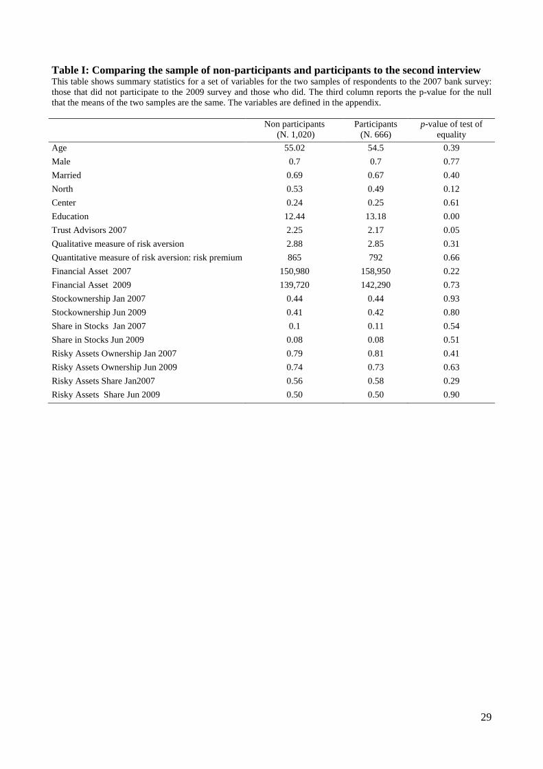
end up with a two-year panel of 666 investors. Table I compares the characteristics of respondents

and non-respondents to the 2009 survey along several dimensions. In the first part of the table, we

compare the two samples according to the demographic characteristics collected in the 2007 survey

such as age, gender, marital status, geographical location, and education. The differences are small

and not statistically significant, with the exception of education where we cannot statistically reject

the hypothesis that the two samples differ. Still the economic magnitude of the difference is small

(less than a year of education).

In the middle part of the table, we compare the two samples according to their risk attitudes,

as measured in 2007. Along this dimension, which is the most important one for our analysis,

participants in the 2009 survey do not differ from non-participants. For instance, the average 2007

2 Since the second survey was filled during the same season as the first, the differences in risk aversion cannot be due to season variations in the length of day (see Kamstra et al. (2003)).

8

risk premium for the hypothetical risky prospect is 865 euros among non-respondents to the 2009

telephone survey and 792 euros among respondents (p-value =0.66).

While the two samples do not differ in observable characteristics in 2007, they might differ

in time-varying characteristics. For example, the crisis might have affected the two groups

differentially, in a way that is correlated with their willingness to be re-interviewed. Fortunately, we

have the 2007 and 2009 administrative data (and hence portfolio choices) of both the respondents

and the non-respondents. Hence, the last part of Table I compares these choices. The stock of

financial assets, before and after the crisis, does not differ between the two groups, nor does the

fraction of financial wealth invested in stock or risky financial assets. Similarly, there are no

differences in the percentage of people who own stock or risky financial assets. From this we

conclude that there does not seem to be any systematic selection in the investors’ decisions to be re-

interviewed in June 2009.

2.2. Our Risk Aversion Measures

As Figure 1a shows, in the 2007 only 16 percent of the sample chooses the “low return and no risk”

answer to the qualitative risk aversion question. So most respondents are willing to accept some risk

if compensated by a higher return, but very few (1.8 percent) are ready to choose very high risk and

very high return. From the answers to this question we construct a categorical variable ranging from

1 to 4 with larger values corresponding to greater risk aversion.

Figure 1b presents the risk premia associated to the answers to the quantitative question.

Interestingly, roughly one third of the respondents appear risk loving in 2007. The extreme risk-

averse people (with a risk premium equal to 4900) are 17% in 2007.

In the 2009 survey we also ask “After the stock market crash did you become more cautious

and prudent in your investment decisions?” The possible answers are: “More or less like before,”

“A bit more cautious,” or “Much more cautious.” Thirty-five percent of the respondents declare to

have become much more cautious, while 18% a bit more. Therefore, we create a “change in

cautiousness” variable equal to zero if the response is no change, 1 if the response is a bit more, and

2 if it is much more. The summary statistics for these measures and all the other variables are

contained in Table II.

2.3 Validating the risk aversion measures

A large and increasing literature shows that questions like the ones above predict risk taking

behavior in various domains (see for instance Dohmen et al. (2011), Donkers et al. (2001), Barsky

et al. (1997), Guiso and Paiella (2006, 2008)). The risk aversion measure elicited in this way are

9

also robust to the specific domain of risk: using a panel of 20,000 German consumers Dohmen et al.

(2011) show that indicators of risk attitudes over different domains tend all to be correlated, with

correlation coefficients of around 0.5 - a feature that is consistent with the idea that risk aversion is

a personal trait.

To validate our measures, we run various tests. First, in Table III we document that our

qualitative and quantitative measures are positively correlated either when using the 2007 cross

section (correlation coefficient 0.12) or the 2009 cross section (correlation 0.16) or when looking at

the correlation between the changes in the two measures between 2007 and 2009 (correlation

coefficient 0.12). We also find that the change in cautiousness variable has a 12% correlation (p-

value 0.002) with the changes in the qualitative measure of risk aversion and a 7.4% correlation (p-

value 0.056) with changes in the quantitative measure of risk aversion.

Second, we document that our measures tend to be correlated in expected ways with

classical covariates of risk attitudes.3 As Panel A of Table IV shows risk aversion decreases with

total wealth levels in both the 2007 and the 2009 cross sections. Also, as documented in the

literature, men are less risk averse than women (Byrnes, 1999).

Third, we document that our measures have predictive power on investors’ financial

choices. Panel B of Table IV shows that the qualitative indicator of risk aversion is strongly

negatively correlated with ownership of risky financial assets (a dummy variable equal 1 if an

individual owns stocks and corporate bonds in her portfolio). The correlation with the lottery-based

measure is negative but weaker. This is partly due to some investors providing noisy answers in the

quantitative measure, which is more difficult to understand. When we drop inconsistent answers -

those who are highly risk averse according to the first indicator (a value greater than 2), but highly

risk lovers on the basis of the lottery question (a risk premium less or equal to -4000 euros) - we

also find that the quantitative measure significantly predicts risky asset ownership. Furthermore, the

change in risk aversion predicts the change in assets ownership: those whose risk aversion increased

more between 2007 and 2009 are more likely to become non-stockholder over the same period

(Table IV.C). In the Appendix (Table A.3 and Table A.4), we also document a similar pattern for

the level and in the change in the share of wealth held in risky assets.

2.4 Changes in wealth and financial losses

For all the participants in the survey, we have access to the administrative data, which include the

amount of deposits at the bank, the amount and composition (by broad categories) of their 3 These patterns of correlations have been documented in several studies, either using surveys or experiments (e.g. Croson and Gneezy (2009) for gender; Barsky et al. (1997), Guiso and Paiella (2006, 2008), Hartog et al. (2002)).

10

brokerage account at the bank, the proportion of financial wealth represented by their holdings at

bank, and the value of their house. Thanks to these data we can infer the changes in respondents’

total wealth and the losses incurred on their financial portfolio. The change in total wealth is

computed as the sum of the actual changes in their financial wealth held at the bank (divided by the

proportion of financial wealth held at the bank to obtain an estimate of total household assets) and

the imputed changes in home equity. To impute these changes we look at the variation in local

indexes of real estate prices. The losses on the financial portfolio are computed by multiplying the

holdings of risky securities (stocks, stock mutual funds, corporate bonds and corporate bonds funds)

before August 2008 by the proportional change in their price between September 2008 (before

Lehman collapse) and February 2009 (when the stock market started to rebound) and then scaling

by the stock of financial assets before August 2008.

3 Changes in Risk Aversion

3.1 Changes in Individual Risk Aversion

Figure 1A compares the distribution of the qualitative measure of risk aversion before and after the

crisis. Before the crisis the average response was 2.87, after the crisis it has jumped to 3.28 (recall, a

higher number indicates higher risk aversion). This change is statistically different from zero at the

1% level. In 2007, only 16% of the respondents chose the most conservative option “low return and

no risk;” in 2009, 43% did. In the Appendix (Table A.5) we show the transition matrix of the

responses. There is a homogenous shift toward more conservative combinations of risk and return.

83% of the people who chose the most aggressive option (“Very high returns, even at the risk of a

high probability of losing part of the principal”) change toward a more conservative one. 74% of

those who had chosen the second more risky combination (“high return and high risk”) move to

more conservative options, while only 2% move to the more aggressive one. 44% of those who

chose “moderate return and moderate risk” move to “low return and no risk,” while only 9.5%

move to more aggressive options. Note that these very stark results are present in spite of a

censoring in the data. The 16% of the respondents who chose the most conservative option in 2007

cannot become more risk averse.4

Figure 1B compares the distribution of the risk premium before and after the crisis and Figure

1C the mean and median risk premium before and after the crisis (the transition matrix is in Table

A.6). As Figure 1C shows, before the crisis the average risk premium investors are willing to pay

4 The effect of this censoring is considered in the Online Appendix.

11

to avoid a gamble offering 10,000 euros and zero with equal probability was 973 euros. In 2009,

the risk premium for the same group of people increased to 2,215 euros. The median increased

from 1,000 to 3,500. All these changes are statistically different from zero. Interestingly, the large

surge in the risk premium is driven by a much higher number of people who choose the lowest

certainty equivalent (and thus the highest risk premium).

Since the risk premium is proportional to the investor risk aversion, these estimates imply that

the (absolute) risk aversion of the average investor has increased by a factor of 2 and that of the

median investor by a factor of 3.5!

One benign reason why risk aversion might have increased is that from the first to the second

survey our respondents became older. While true, this effect is likely to be small, since only two

years went by. Nevertheless, we computed the average risk aversion by age and then took the

difference of risk aversion between the first and the second survey keeping the age constant (i.e.

between the average of people who were thirty in 2009 and the people who were thirty in 2007).

The results are unchanged.

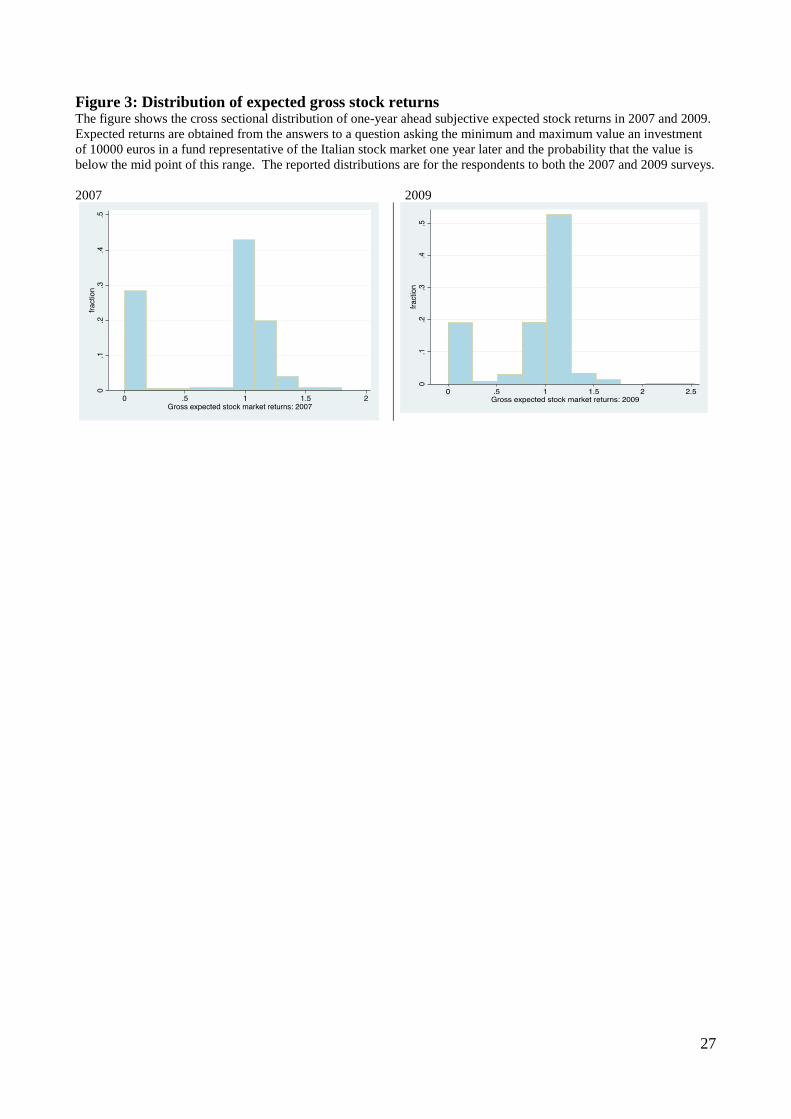
This increase cannot be attributed solely to a worsening of expectations about the distribution of

future investments since it manifests itself also in the quantitative measure, which is unrelated to the

stock market. In fact, the probability distribution underlying the gamble in the quantitative measure

is objective, not subjective. For the qualitative one, we report the distribution of expected returns.

As one can see in Figure 3, the left tail has not become fatter in 2009 and the subjective probability

of the worst outcome (total loss) has not increased after the crisis. This finding is inconsistent with

the extreme outcome hypothesis.

3.2 Portfolio Rebalancing

Did this large change in risk aversion affect portfolio choices? In Table IV.C we have shown

that there is a correlation between the changes in the share of risky assets and the changes in

individual risk aversion. Our sample, however, allows us to go deeper. We have the active

portfolio decisions, so we can test whether the individual changes in risk aversion predict active

portfolio rebalances after the crisis.

Let assume that before the crisis individual portfolios were at the optimal Mertonian share

. This assumption is realistic given that before the crisis stock prices were fairly flat for

a while and thus investors did have all the time to adjust. Denote with p the value of stocks after

the shock relative to their value before, p < 1. Then, after the severe market downturn the actual

share of risky assets became

2

eMi

i

rωγ σ

=

12

We have seen that after the crisis the distribution of expected returns did not change. If the

individual risk aversion did not change either, the portfolio rebalancing of individual i would be

given by

(1)

If the risk aversion moves to , then the portfolio rebalancing of individual i is

(2) .

We can nest these two specifications as

(3)

where if , , we obtain (1), i.e., the optimal rebalancing under the standard

Mertonian model with no changes in risk aversion, while if , , we obtain (2), i.e.

the optimal rebalancing when the risk aversion parameter changes.

To test which expression fits the data best we build empirical counterparts of the terms on

the right hand side of (3); the details are reported in Appendix A4. We define the shock as the drop

in stock prices that occur after August 2008, i.e. the pre-Lehman month. Since prices continue to

fall until February 2009 we define various measures of the drop in risky asset prices since August

2008 computed at different months from September 2008 until February 2009. Importantly, we

construct an investor specific measure of p by taking portfolio-weighted means of the drop in

different components of the risky portfolio using as weights the risky portfolio compositions of

each individual as of August 2008. is computed as the net flow of risky assets (positive for net

purchases and negative for net sales), scaled by the value of total financial assets in August 2008.

The results are reported in Table V. In all regressions we add some demographic controls

and the change in total assets; results are invariant to these controls. The left hand side variable

represents the active reallocation in the period that goes from August 2008 to the date written at the

top of each column. Thus, in column 1 the reallocation considered is the one during the period

August ’08 to September ’08. In all the specifications except one the coefficient is significantly

bigger than zero, albeit also significantly less than 1. In all the specifications the coefficient is not

different from zero, while the coefficient is negative and sometimes significantly different from

1

Mi

i M Mi i

pp

ωωω ω

=+ −

1

MM i

i i M Mi i

pRp

ωωω ω

= −+ −

'iγ

' 1

MMi i

i i M Mi i i

pRp

γ ωωγ ω ω

= −+ −

'[ 1] [ ] [ ]1

MM Mi i

i i i M Mi i i

pRp

γ ωα ω β ω δγ ω ω

= − + ++ −

0α = 1β = 1δ = −

1α = 0β = 1δ = −

( )iR t

α

β

δ

13

zero, albeit always significantly different from -1. Thus, none of the two models perfectly fits the

data. Yet, considered that the noise in the data tends to downward bias the coefficient, the data

seems more consistent with model (2) – where the changes in risk aversion impact the portfolio

rebalancing—than with model (1).

3.3 A Reality Check on the Magnitude of the Changes

Our sample is representative of Italian individual investors, but not of all investors: institutional

investors and professional traders are not represented. Yet, if we treat it as a representative sample,

we can compute the aggregate risk aversion and check whether the change in the aggregate risk

aversion is large enough to explain the large drop in stock prices.

To compute the aggregate risk aversion we start by mapping the risk premium computed from

the quantitative question into a coefficient of absolute risk aversion by using a CRRA utility

function. Then, we compute the aggregate risk aversion by weighting these coefficients by the net

total wealth of each individual. As Table VI shows the aggregate risk aversion in 2007 was 1.3. If

we maintain the individual risk aversions estimated in 2007 and multiply them by the 2009 wealth

weights, the aggregate risk aversion does not change at all. By contrast, if we use the 2009

estimated individual risk aversion, the aggregate risk aversion almost doubles. If we repeat the

analysis restricting the sample to people who were stockholders in 2007 the results are the same.

Now that we have computed the variation in aggregate risk aversion, we can estimate whether

this change is sufficient large to justify the severe drop in stock prices that took place. What is

relevant for asset prices is the relative risk aversion. Since the change in total wealth is small (a

relatively small fraction was invested in equity), all the increase in absolute risk aversion translates

into an increase in the relative risk aversion. To compute how this increase could affect stock prices

we make the (strong) assumption that the only source of variation was a (temporary) increase in risk

aversion. This implies that the future expected cashflow remains unchanged and that after one year

even the risk aversion returns to normal. Then, next year stock price 1P should remain unchanged

and all the adjustment should take place in today’s stock price 0P . By using the Merton (1969)

model, we can write

where the left hand side is the equity premium and 2σ the variance of stock returns. If risk aversion

doubles to =2 , as it does in our sample, then the initial stock price '0P should be

14

,

which is roughly half of what it was before. Hence stock price roughly halves if risk aversion

doubles. Thus, the sharp increase in risk aversion is quantitatively sufficient to explain the severe

drop in stock prices during the crisis. Yet, it begs the question of what caused this increase in risk

aversion.

4 What Explains the Changes in Risk Aversion?

A characteristic that standard expected utility models have in common with the non-standard

ones is that any change in risk aversion is mediated by changes in wealth. For this reason, we start

by plotting a non-parametric estimation of the relationship between changes in risk aversion (both

the qualitative and the quantitative measures) and the size of financial losses incurred between

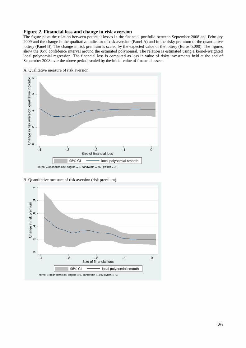
September 2008 and February 2009 (if we use total wealth the results are the same). As Figure 2a

shows, there is no consistent relationship between the increase in the qualitative measure of risk

aversion and the size of the losses in the financial portfolio during the financial crisis. For losses

between zero and 20%, the increase in risk aversion is stable at 0.4, around 14% of the sample mean

in 2007. For losses above 20%, the increase in risk aversion seems to first decrease and then

increase.

As Figure 2b shows, for the quantitative measure there seems to be a negative relation

between the size of the financial loss and the relative risk premium (the risk premium divided by the

expected value of the lottery), which is consistent with NSEU models. Yet, even people with no

losses exhibit a significant increase in the relative risk premium (by 20 percentage points), which

seems at odd with NSEU models.

To better understand the robustness of these results we focus on the 295 people who did not

experience any financial loss between September 2008 and February 2009 (either because they

gained or because they did not have any risky assets and thus did not experience any loss).5 Before

the crisis the qualitative measure of risk aversion of this subsample was 2.82 (statistically not

5 The people with inconsistent answers are 59. We focus on financial losses; households could have suffered losses on housing wealth. This is not the case: between the second quarter of 2009 and the first quarter of 2008 house prices increased in all local markets but one where they dropped by 3.7%. A non parametric estimate of the relation between the change in the qualitative and quantitative measures of risk aversion and the proportional change in total wealth leads to a similar conclusion. The certainty equivalent increases by a similar amount even for households whose total wealth holdings do not change or even increase.

15

different from the rest of the sample). After the crisis their qualitative measure jumped to 3.25,

again not statistically different from the jump in the rest of the sample.

The same is true for the quantitative measure. Before the crisis the mean risk premium for

this subsample was €831, not statistically different from the rest of the sample. After the crisis, the

mean risk premium rises to €2,260, not statistically different from the rest of the sample. Therefore,

investors who did not experience any loss exhibit an increase in risk aversion equal to those who

did.

One possible explanation is that investors are responding to a change in the background risk

caused by the crisis. The income from financial assets is generally small relative to labor income. If

there is a significant change in the labor income risk, this might affect the measured risk aversion.

For this reason we focus on people who face much less (possibly no) labor income risk.

People in the first category are government employees. Note that 2009 predates the Greek and euro

crisis and the Italian government solvency was not seriously in doubt (at that time the spread

between the 5 year Italian bond and the German one was around 60 basis points). As Table VII

shows, government employees who did not face any financial loss still exhibit a surge in risk

aversion (both the qualitative and quantitative measures), which is statistically different from zero.

Interestingly, if we compare the surge in risk aversion between government employees who did not

face any financial loss and non-government employees who did not face any financial loss, we find

no difference, casting doubts that background risk can explain the surge.

Our measure of financial losses is based on the wealth investors have deposited at the Bank.

We cannot exclude, thus, that they might have faced a loss in other investments. For this reason, in

the third and fourth rows of Table VII we restrict the attention to individuals who declare that they

only have financial wealth at the Bank (144 observations). The results are very similar. In fact, if

anything the qualitative and quantitative measures of risk aversion increase by more among

government employees than non-government employees.

We repeat the same analyses dividing the sample of investor who did not face financial

losses between retirees and non retirees. In Italy retirees enjoy a defined benefit plan backed by

government guarantee. Thus, the same considerations above apply. We find no difference between

the surge in risk aversion of retirees and non retirees.

Yet, it is still possible that risk aversion changes because individuals perceive an increased

background risk, which is hard to measure. For example, even a retiree, with a fully guaranteed

pension, may rely on his children’s income as potential insurance against idiosyncratic shocks. If

the financial crisis reduces the children’s expected income, it might increase the value function’s

risk aversion of the parents.

16

Another possibility is that the surge in absolute risk aversion is due to a large non-financial

loss, such as a permanent reduction in labor income. If we use a standard CRRA utility model, we

need a 50% reduction in future labor income to account for a doubling of the absolute risk aversion.

Such a large drop is unlikely, especially for government employees or for retirees. In a habit

persistence model, however, a much lower reduction of permanent income is able to account for a

doubling of the absolute risk aversion.

Yet, if this is the reason for the surge in risk aversion, risk aversion should increase much

more for younger people (who have most of their wealth in human capital) than for older people. To

analyze this possibility, in the bottom part of Table VII we split the sample of people who did not

suffer any financial loss between young (age below 45) and old (age above 65). The change in

qualitative risk aversion is the same for the two groups, while the change in the quantitative

measure is larger for older people than for younger ones.

In Table VIII we repeat all this analysis in a regression form. The results are the same. In

sum, we document that people become more risk averse because of a state variable in the

environment that has little or nothing to with their own personal present and future wealth.

Therefore, they might respond to losses of their friends and neighbors, rather than to an internal or

external habit. While this possibility is consistent with Delong et al. (1990) idea of sentiment, its

working has not been explicitly modeled in the financial literature. It has been developed, however,

in the psychology literature by Lowenstein (1996, 2000) and Loewenstein et al. (2001). 4.3 The Fear Alternative

Most of the economic models treat emotions as part of the utility function: feelings are expected

consequences of the outcomes and are taken into account in decision making through a cognitive

process. Alternatively, Loewenstein et al. (2001) recognize that emotions are often experienced at

the time of the decision and may lead to action bypassing the cognitive process. In this framework,

visceral factors (Loewenstein, 1996, 2000), such as fear, may alter behavior rapidly. Emotions

originate in the brain’s limbic system (amygdala, cingulate gyrus and hippocampus) and they are

processed and moderated by the frontal cortex (Pinel, 2009). A simple way to embed the role of

emotions in the standard utility framework is to assume that emotions can alter a parameter of an

individual utility function. Thus, we interpret fear as a state-contingent increase in the curvature of

the utility function.

This hypothesis can explain why, in the 2008 financial crisis context, investors who did not

lose any money became more risk averse even with respect to known probabilities gamble such as

our quantitative measure. The terrifying news appearing on television, the interaction with friends

17

who lost money in the market, the pictures of fired people leaving their failed banks might have

triggered an emotional response.

While suggestive, this hypothesis cannot be tested with our data because it is observationally

equivalent to a background risk model. Does the TV reporting of Lehman’s fired employees trigger

an emotional fear response or does it increase the subjective probability of a very bad outcome?

And if it triggers a fear response is this sufficiently strong to explain the increase in risk aversion

that we have documented in Section 3?

5 Fear-Inducing Experiment

5.1 The advantage of a laboratory experiment

With non-experimental data, it is impossible to separate the emotional response from a Bayesian

response, based on an updated probability of a large disaster (a revolution, a Great Depression, etc.)

or an increase in a non-measurable background risk. Indeed, individuals might be reluctant to take

risks because they believe that the realization of extreme events is now more likely (e.g., Caballero

and Krishnamurthy, 2009) or because they overestimate the realization of negative outcomes.

To separate the emotional response from a Bayesian response and establish whether an

emotional response can generate large increases in risk aversion, we rely on a laboratory experiment

where the outside environment is controlled for. As long as the treatment provides no information

about the real world, the probability of an extreme event should remain constant between treated

and untreated samples. To discriminate between the two hypotheses, thus, the key feature of such an

experiment is to induce fear in the lab without altering a subject’s perception of her financial and

economic prospects. To achieve this goal we rely on the fear conditioning model used in

psychology. Notice that our intent is not to prove whether fear causes an increase risk aversion. This

link has already been established (see e.g. Cohn et al (2014)). Our purpose is to test whether the fear

channel is powerful enough to generate an increase in risk aversion of a magnitude that resembles

the one induced by the financial crisis.

5.2 The fear conditioning model

As for the classical Pavlov (1927) experiment, the fear response can be triggered by

conditioning factors, which have little or nothing to do with the experience itself. As Pavlov’s dog

salivates when a bell rings, the fear response arises in the presence of stimuli associated to past

traumatic events. This evidence suggests that a fear-based response can be triggered by fear stimuli

in an unrelated domain. For example, Kinreich et al. (2012) show that watching a horror movie

18

stimulates the amygdala in a way consistent with the arousal of fear. Yet, they do not provide

evidence that this experience can alter a risk aversion measure like ours, nor that it can alter it to the

extent we observe after the financial crisis. This is what we try to test.

We chose a brief horrifying scene from a movie that was sufficiently recent to be really

scary for undergraduates used to the scariest videogames (Psycho would not cut it), but sufficiently

old to minimize the chance they had already seen it. We chose a five-minute excerpt from the 2005

movie, Hostel, directed by Eli Roth, which is characterized by stark and graphic images and that

show a young man inhumanly tortured in a dark basement. This movie won "Best Horror" at the

Empire Awards in 2007.

Our experiment was run at Northwestern University in March 2011 in three different

sessions. A total number of 249 students took part. The participants were recruited through an

internal mailing list service that is normally employed for experiments at Northwestern.6 A

compensation of $5 was paid in cash to each subject taking part in the experiment, which in general

takes around 10-15 minutes.

All the participants were asked to complete a questionnaire of approximately 40 questions.

The main scope of this is to construct some measures of risk aversion, as well as to provide other

controls. In order to identify the effect of fear on the subjects, we relied on a simple treatment and

control framework. In particular, around half of the participants were asked to watch a short video

before completing the questionnaire. Since the subjects were randomly assigned to watch the video,

the idea is that the difference in risk aversion between the two groups should be completely driven

by this difference in the treatment.

Given the nature of the video, which potentially disturbs some of the subjects, we had to

give them the option to skip the video at any moment. We dropped the observations of the subjects

(27) who decided to skip the video in the first minute of the five minute presentation, since they did

not really experience much horror. This choice might underestimate the effect of the treatment,

since those most sensitive to the treatment dropped out.

Another possible concern is that, if a subject has already watched the video, its perceived

effect would be different from the true effect. We therefore decide to drop those 13 subjects who

declared to have already watched it.

In order to guarantee the reliability of the results, the experiment was designed in such a

way that the participants were not aware that the treatment was not identical for everyone. As

6 The students can freely enroll to the mailing list and, after they have completed an introductory demographic survey, they receive periodic communications on the experiments that are going on at the University.

19

measures of risk aversion, we use answers to the very same questions that were used in the bank

survey, where we translated euro into dollars at a 1:1 ratio.

As Table IX shows, the random assignment assumption cannot be rejected: none of the main

personal characteristics and demographic information has been found to be statistically different

between treatment and control groups. Furthermore, around 40% of the participants were female

and the average age is 20, which is not surprising given that the sample is composed of

undergraduate students.

When we look at the risk aversion measure, we find that there is a large and statistically

significant difference in the quantitative measure of risk aversion. Among the treated students the

risk premium they are willing to pay for avoiding the risky lottery is $672 (i.e., 27%) higher. This

holds true without controls and controlling for observables (Table A.8).

In the qualitative measure we observe a drop, but this drop is not statistically significant at

the conventional level (p-value =0.111). In part, this phenomenon is due to the fact that students

bunched their choices in the two central values: 96% of the responses are either 2 or 3. Hence, the

scale 1-4 is probably better reduced to a dichotomous choice: low risk aversion (1 and 2) and high

risk (3 and 4). When we look at the proportion of people choosing the low risk option, this

proportion increases by 13.5 percentage points (30% of the sample mean) among the treated group.

This difference is large and statistically significant at the 5% level.

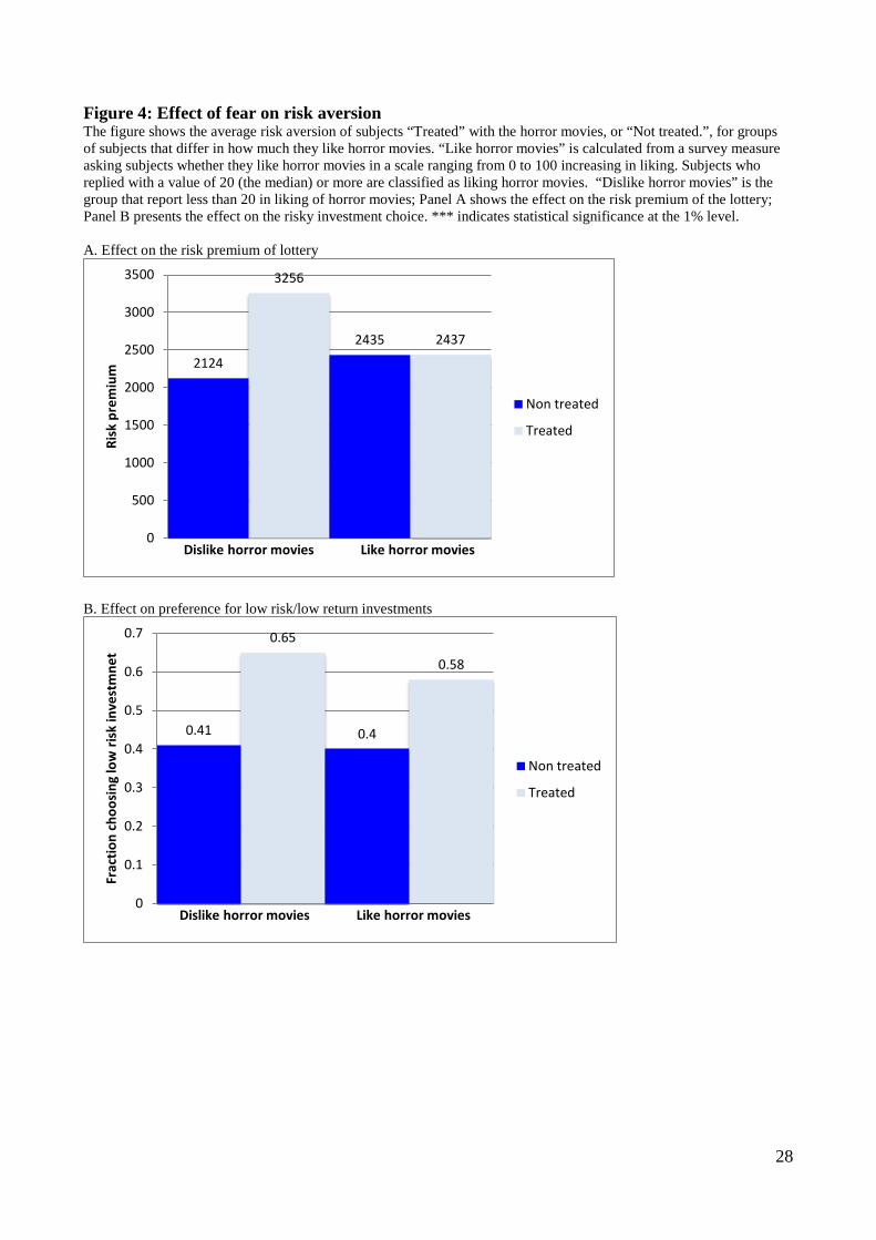
In the second half of the sample, we asked people how much they liked horror movies on a scale

from 0 to 100. Roughly a third of the sample declared they do not like it at all (i.e., like=0) and 50%

report a value of liking below 20. In Figure 5 we split the sample on this basis. In the first group,

there are students who do not like horror movies (liking indicator below median). Their risk

premium rises from $2,124 to $3,256 as a result of the treatment (Panel A). This difference is

statistically significant at the 1% level.

The second group is formed by those subjects who moderately like horror movies ((liking

indicator above 20). Here the treatment has a no effect (the risk premium goes from 2,435 to 2,437)

and this difference is not statistically significant.

We get a similar result when we look at the qualitative measure of risk aversion, where we

bunched the responses into two groups. Among people who dislike horror movies the treatment

effect increases the probability of buying risky assets by 25 percentage points. Among those who

moderately like horror movies the increase is significantly smaller by 7 percentage points.

7. Conclusions

20

By using a survey based measure we find that investors’ risk aversion increases significantly

between 2007 and 2009. This increase is present even among those investors who did not

experience any financial loss. This evidence is consistent ewith a change in unobserved background

risk, with a change in the perceived probabilities of a catastrophe, or with a surge in what

psychologists call fear that we interpret as a state-contingent change in the curvature of risk

aversion. Since these alternatives cannot be disentangled with field data, we rely to a lab experiment

for identification. In this setting we can keep constant wealth, background risk, and perceived risk

of a catastrophe and isolate the potential effect of fear. We find that the students treated with a scary

movie exhibit a significant increase in risk aversion, similar in magnitude to the one observed in the

data. This seems to be inconsistent with the background risk and the perceived probability of a

disaster hypotheses, unless we espouse a behavioral interpretation: exposure to scary events/images

increases the salience (Bordalo et al, 2012) of negative outcomes and thus their perceived

probability.

In our view, the paper has two main contributions. The first is methodological. Most papers

use either naturally occurring data or lab/field data, but not both. We think that well designed lab

test can be a useful complement to the analysis of naturally occurring data, when we are faced with

very important questions that are impossible to answer with naturally occurring data. In particular, it

is impossible to disentangle whether the surge in risk aversion we observe in the data is due to fear

or background risk. If we were unable to reproduce that surge in the lab, we could have ruled out

the fear explanation. The fact we were unable to does not prove that the cause of the surge in the

data is fear, but it makes it more plausible. Thus, targeted lab experiments can help in identifying

effects difficult to sort out in naturally occurring data.

The second contribution is to provide some evidence consistent with a fear-based

explanation of the increase of risk aversion during the financial crisis. This evidence is not in

contradiction with the “institutional finance” hypothesis (e.g., Vayanos, 2004; He and

Krishnamurthy, 2012), which attributes the rise in aggregate risk aversion during the crisis to an

increase in the leverage of financial intermediaries. In fact, we see the two hypotheses as

complementary. A surge in individual risk aversion can have no impact on prices as long as

institutional investors are not highly leveraged and can absorb the sales by scared individuals.

However, when institutional investors do not have this flexibility, individual panic might affect

prices. How these two ideas can be combined is left for future research.

A question we are unable to answer in this paper is how persistent such fear-induced change

in risk aversion is. The evidence of Malmendier and Nagel (2011), who find a cohort effect of

“Depression era babies” in the risk aversion measure of the Survey of Consumer Finances, suggests

21

it might be long-lasting. With our sample we are unable to answer whether fear provokes long term

consequences because of the subsequent events in the Eurozone, which made the 2008 shock not an

isolated crisis.

Finally, our results raise an interesting question. If the behavior we document is typical and

during severe downturns investors are caught by fear and sell their risky assets at the worst times,

the effective return on equity investment is much lower. Can this feature explain – at least in part--

the famous equity premium? Only future research would be able to tell.

22

References

Baker Malcolm and Jeffrey Wurgler (2007) Investor sentiment and the Stock Market, Journal of Economic Perspectives, Volume 21, Number 2, 129–151.

Barberis Nicholas, Ming Huang, and Tano Santos (2001) "Prospect Theory and Asset Prices," Quarterly Journal of Economics 116, 1-53,

Barsky, Robert. B., Thomas F. Juster, Miles S. Kimball, and Mathew D. Shapiro (1997): “Preference Parameters and Individual Heterogeneity: An Experimental Approach in the Health and Retirement Study,” Quarterly Journal of Economics, 112(2), 537–579.

Basi, Ana, Ricardo Colacito and Paolo Fulghieri (2013). “O Sole Mio. An Experimental Analysis of Weather and Risk Attitudes in Financial Decisions”, Review of Financial Studies, 26(7): 1824–1852.

Bombardini, Matilde and Francesco Trebbi, (2011), “Risk aversion and expected utility theory: A field experiment with large and small stakes”, Journal of the European Economic Association, forthcoming.

Bonaparte, Yosef and Russel Cooper (2010), “Costly Portfolio Adjustment," NBER Working paper 15227. Bordalo, Pedro, Nicola Gennaioli, and Andrei Shleifer. 2012. “Salience Theory of Choice under Risk.” Quarterly Journal of Economics 127 (3):1243–85.

Brunnermeir, Markus and Stefan Nagel (2008), "Do Wealth Fluctuations Generate Time-varying Risk Aversion? Micro-Evidence on Individuals' Asset Allocation," American Economic Review, 2008, 98(3), 713-736

Byrnes JP, Miller DC, Schafer WD. (1999) Gender differences in risk taking: A meta-analysis. Psych Bull.;125:367–383.

Caballero, Ricardo J. and Arvind Krishnamurthy, 2009, Global Imbalances and Financial Fragility, American Economic Review, Vol. 99, Issue 2, Pages 584-588.

Campbell, John and John Cochrane, 1999, “By Force of Habit: A Consumption-Based Explanation of Aggregate Stock Market Behavior,” Journal of Political Economy, 107, 205-251 (April 1999). Campbell, John Y., Stefano Giglio, and Christopher Polk, 2011, “Hard Times” Harvard University working paper. Cohn, Alain, Jan Engelmann, Ernst Fehr, and Michel André Maréchal. 2015. "Evidence for Countercyclical Risk Aversion: An Experiment with Financial Professionals." American Economic Review, 105(2): 860-85

Croson, Rachel and Uri Gneezy (2009), "Gender Differences in Preferences", Journal of Economic Literature, 47:2, 1{27}.

23

DeLong, J. Bradford, Andrei Shleifer, Lawrence H. Summers, and Robert J. Waldmann (1990), “Noise Trader Risk in Financial Markets.”Journal of Political Economy, 98(4): 703–38.

Dohmen, Thomas Armin Falk, David Huffman, Uwe Sunde, Jürgen Schupp, Gert G. Wagner (2011),” Individual Risk Attitudes: New Evidence from a Large, Representative, Experimentally-Validated Survey”, Journal of the European Economic Association, forthcoming

Donkers, B., B. Melenberg, and A. V. Soest (2001): “Estimating Risk Attitudes Using Lotteries: A Large Sample Approach,” Journal of Risk and Uncertainty, 22(2), 165–195.

Friend Irwin and Marshall E Blume, 1975, The Demand for Risky Assets, American Economic Review, 1975, vol. 65, issue 5, pages 900-922

Guiso, Luigi and Monica Paiella (2006), “The Role of Risk Aversion in Predicting Individual Behavior”, in Pierre-André Chiappori and Christian Gollier (editors), Insurance: Theoretical Analysis and Policy Implications, MIT Press, Boston.

Guiso, Luigi and Monica Paiella (2008), “Risk Aversion, Wealth and background Risk”, Journal of the European Economic Association, 6(6):1109–1150

Hartog, Joop, Ada Ferrer-i-Carbonell, and Nicole Jonker, (2002), "Linking Measured Risk Aversion to Individual Characteristics." Kyklos, 55(1): 3-26.

Heaton John and Deborah Lucas, 2000, "Portfolio Choice in the Presence of Background Risk," Economic Journal, 2000, 110(460), pp. 1-26.

Holt, Charles A. and S.K. Laury, (2002), “Risk aversion and incentive effects”, American Economic Review 92 (5), 1644-1655.

Kamstra, Mark J., Lisa A. Kramer, And Maurice D. Levi, 2003,“Winter Blues: A SAD Stock Market Cycle”, American Economic Review, Vol. 93 No. 1

Knutson, B., E. Wimmer, C. M. Kuhnen, and P. Winkielman, ”Nucleus Accumbens Activation Mediates Reward Cues’ Influence on Financial Risk-Taking,” NeuroReport, 19 (2008), 509-513.

Kramer Lisa A. and J. Mark Weber, 2012, “This is Your Portfolio on Winter: Seasonal Affective Disorder and Risk Aversion in Financial Decision Making,” Social Psychological and Personality Science 3(2) 193-199.

Kuhnen, Camelia M. and Brian Knutson, 2005, “The Neural Basis of Financial Risk Taking,” Neuron, Volume 47, Issue 5, 763-770, 1 September 2005.

Kuhnen, Camelia M. and Brian Knutson, (2011), “The Impact of Affect on Beliefs, Preferences and Financial Decisions.” Journal of Financial and Quantitative Analysis, 46 (3): 605-626, June 2011

Kinreich, Sivan, Nathan Intrator, and Talma Hendler, 2012, “Functional Cliques in the Amygdala and Related Brain Networks Driven by Fear Assessment Acquired During Movie Viewing” Brain Connectivity. Lerner, Jennifer S. and Dacher Keltner, D. (2000). Beyond valence: Toward a model of emotion- specific influences on judgment and choice. Cognition and Emotion, 14, 473-494.

24

Lerner, Jennifer S. and Dacher Keltner, (2001), “Fear, Anger, and Risk,” Journal of Personality and Social Psychology, 2001. Vol. 81. No. 1, 146-159 Loewenstein, George (1996), Out of Control: Visceral Influences on Behavior, Organizational Behavior and Human Decision Processes, 65(3) March, 272–292. Loewenstein, George (2000), Emotions in economic theory and economic behavior, The American Economic Review; May (90): 2, 426-432. Loewenstein, G. F., Weber, E. U., Hsee, C. K., & Welch, N. (2001). “Risk as feelings,” Psychological Bulletin, 127, 267-286. Malmendier, U., and S. Nagel, 2011, Depression Babies: Do Macroeconomic Experiences Affect Risk-Taking?, Quarterly Journal of Economics, 126, 373-414. Martin, Ian, 2013, “Simple Variance Swaps”, January, 2013, NBER Working Paper 16884. Merton, Robert C. (1969): Lifetime Portfolio Selection under Uncertainty: The Continuous Time Case, Review of Economics and Statistics, 50, 247–257. Narayanan Kandasamy, Ben Hardy, Lionel Page, Markus Schaffner, Johann Graggaber, Andrew S. Powlson, Paul C. Fletcher, Mark Gurnell, and John Coates (2014). “Cortisol shifts financial risk preferences”, Proceedings of the National Academy of Sciences of the United States of America, 111 (9) 3608-3613. Pavlov Ip, 1927, Conditional Reflex, An Investigation of The Psychological Activity of the Cerebral Cortex, New York, Oxford University press. Pinel, John P.J., 2009, Biopsychology Seventh Edition. Pearson Education Inc. Vayanos Dimitris, 2004, Flight to Quality, Flight to Liquidity, and the Pricing of Risk, Working paper. Weber, Martin, Weber, Elke U. and Nosic, Alen, Who Takes Risks When and Why: Determinants of Changes in Investor Risk Taking, Current Directions in Psychological Science, 20, 211-216.

25

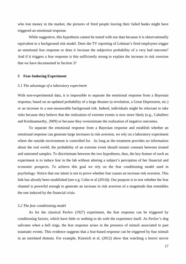
Figure 1: Frequency distribution of the level of risk aversion indicators in 2007 and 2009 Panel A reports the frequency distribution of the qualitative measure of risk aversion in 2007 and 2009. The qualitative indicator elicits the investment objective of the respondent, offering them the choice among “Very high returns, even at the risk of a high probability of losing part of my principal”; “A good return, but with an ok degree of safety of my principal;” “An ok return, with good degree of safety of my principal,” “Low returns, but no chance of losing my principal.” Responses are coded with integers from 1 and 4, with a higher score indicating a higher aversion to risk. Panel B shows the frequency distribution of the risk aversion indicator based on the answers to the lottery that delivers 10,000 euros or zero with equal probability in 2007 and 2009. The risk premium for this gamble is computed as the difference between the expected value of the lottery (5,000€) and each respondent’s certainty equivalent. Panel C reports the average and median risk premium for this gamble in the two years. A. Qualitative measure of risk aversion

B. Quantitative measure of risk aversion (risk premium)

C. Quantitative measure of risk aversion (risk premium) over time Mean

Median

973

2215

0

1000

2000

3000

Risk

Pre

miu

m:

mea

n

2007 2009

1000

3500

0

2000

4000

Risk

Pre

miu

m:

Med

ian

2007 2009

26

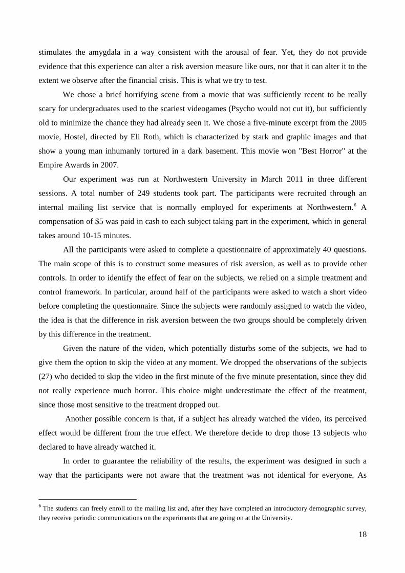
Figure 2. Financial loss and change in risk aversion The figure plots the relation between potential losses in the financial portfolio between September 2008 and February 2009 and the change in the qualitative indicator of risk aversion (Panel A) and in the risky premium of the quantitative lottery (Panel B). The change in risk premium is scaled by the expected value of the lottery (Euros 5,000). The figures show the 95% confidence interval around the estimated polynomial. The relation is estimated using a kernel-weighted local polynomial regression. The financial loss is computed as loss in value of risky investments held at the end of September 2008 over the above period, scaled by the initial value of financial assets. A. Qualitative measure of risk aversion

B. Quantitative measure of risk aversion (risk premium)

27

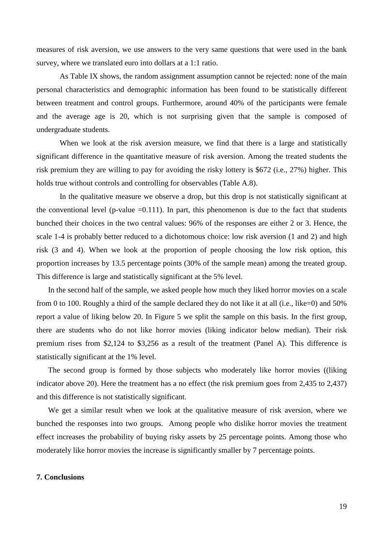
Figure 3: Distribution of expected gross stock returns The figure shows the cross sectional distribution of one-year ahead subjective expected stock returns in 2007 and 2009. Expected returns are obtained from the answers to a question asking the minimum and maximum value an investment of 10000 euros in a fund representative of the Italian stock market one year later and the probability that the value is below the mid point of this range. The reported distributions are for the respondents to both the 2007 and 2009 surveys. 2007 2009

28

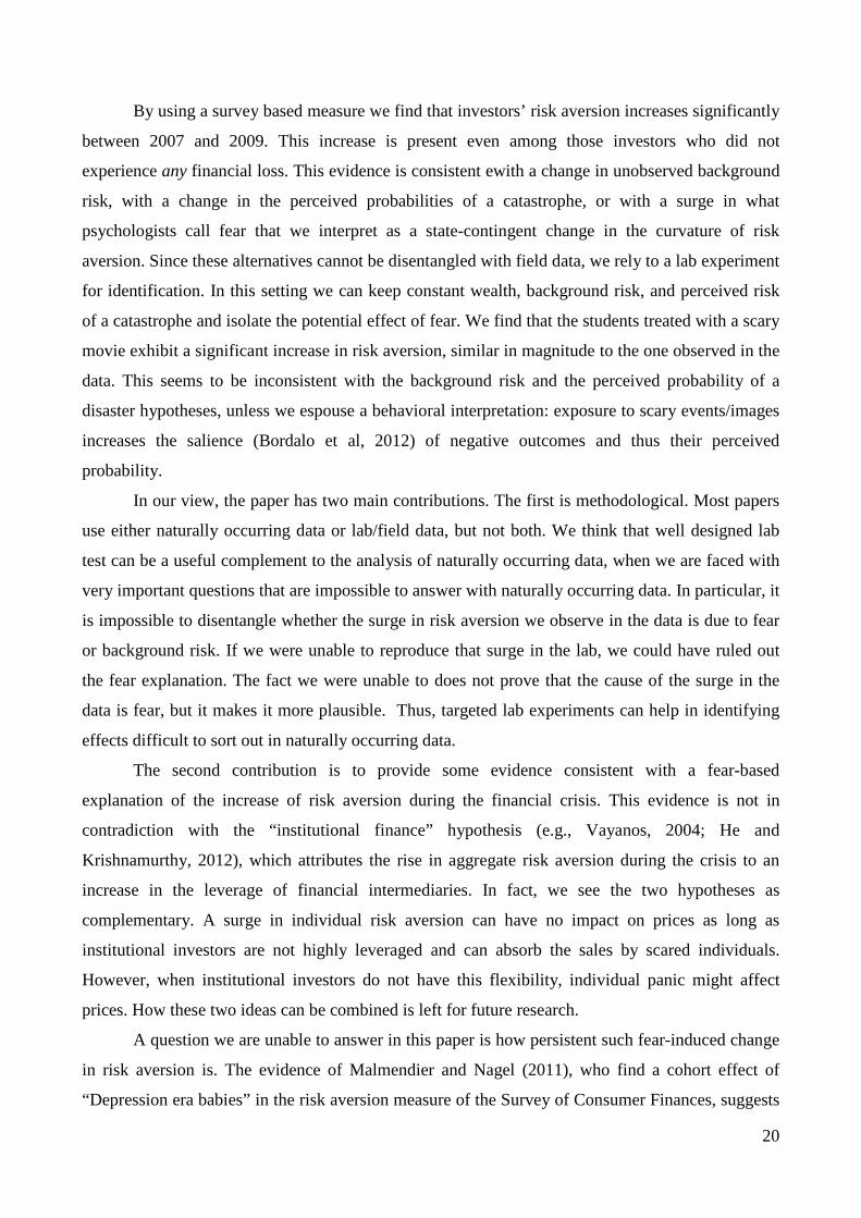
Figure 4: Effect of fear on risk aversion The figure shows the average risk aversion of subjects “Treated” with the horror movies, or “Not treated.”, for groups of subjects that differ in how much they like horror movies. “Like horror movies” is calculated from a survey measure asking subjects whether they like horror movies in a scale ranging from 0 to 100 increasing in liking. Subjects who replied with a value of 20 (the median) or more are classified as liking horror movies. “Dislike horror movies” is the group that report less than 20 in liking of horror movies; Panel A shows the effect on the risk premium of the lottery; Panel B presents the effect on the risky investment choice. *** indicates statistical significance at the 1% level. A. Effect on the risk premium of lottery

B. Effect on preference for low risk/low return investments

2124

3256

2435 2437

0

500

1000

1500

2000

2500

3000

3500

Risk

pre

miu

m

Dislike horror movies Like horror movies

Non treated

Treated

0.41

0.65

0.4

0.58

0

0.1

0.2

0.3

0.4

0.5

0.6

0.7

Frac

tion

choo

sing

low

risk

inve

stm

net

Dislike horror movies Like horror movies

Non treated

Treated

29

Table I: Comparing the sample of non-participants and participants to the second interview This table shows summary statistics for a set of variables for the two samples of respondents to the 2007 bank survey: those that did not participate to the 2009 survey and those who did. The third column reports the p-value for the null that the means of the two samples are the same. The variables are defined in the appendix. Non participants

(N. 1,020) Participants

(N. 666) p-value of test of

equality Age 55.02 54.5 0.39 Male 0.7 0.7 0.77 Married 0.69 0.67 0.40 North 0.53 0.49 0.12 Center 0.24 0.25 0.61 Education 12.44 13.18 0.00 Trust Advisors 2007 2.25 2.17 0.05 Qualitative measure of risk aversion 2.88 2.85 0.31 Quantitative measure of risk aversion: risk premium 865 792 0.66 Financial Asset 2007 150,980 158,950 0.22 Financial Asset 2009 139,720 142,290 0.73 Stockownership Jan 2007 0.44 0.44 0.93 Stockownership Jun 2009 0.41 0.42 0.80 Share in Stocks Jan 2007 0.1 0.11 0.54 Share in Stocks Jun 2009 0.08 0.08 0.51 Risky Assets Ownership Jan 2007 0.79 0.81 0.41 Risky Assets Ownership Jun 2009 0.74 0.73 0.63 Risky Assets Share Jan2007 0.56 0.58 0.29 Risky Assets Share Jun 2009 0.50 0.50 0.90

30

Table II: Summary statistics of risk aversion measures, other variables and controls Panel A reports the summary statistics for the risk aversion measures. The qualitative measure of risk aversion elicits the investment objective of the respondent, offering them the choice among “Very high returns, even at the risk of a high probability of losing part of the principal;” A good return, but with an ok degree of safety of the principal;” “A ok return, with good degree of safety of the principal,” “Low returns, but no chance of losing the principal.” The responses are coded with integers from 1 to 4, with a higher score meaning a higher risk aversion. The quantitative measure of risk aversion is calculated by eliciting the certainty equivalent for a gamble that delivers either 10,000 euro or zero with equal probability; the risk premium is then obtained as the difference between the expected value of the gamble (5,000 Euro) and each respondent’s certainty equivalent. Panel B, C and D report the summary statistics for all the other variables used later in estimates and defined in the Appendix. A. Risk aversion measures in 2007 and 2009 Quantitative measure

(risk premium in euros) Qualitative measure

Mean Median Sd Mean Median Sd Level in 2007 792 1,000 3,248 2.87 3 0.72 Level in 2009 2,215 3,500 2,815 3.28 3 0.73 Change 2009/2007 1,423 2,500 3,994 0.42 0 0.81 Fraction of People with Increase in Risk Aversion 0.55 0.46

Fraction of People with Unchanged Risk Aversion 0.18 0.44

1- Fraction of People with a decrease in Risk Aversion 0.73 0.90

B. Other variables: levels Mean Median Sd Male 0.70 1 0.46 Age 54.81 57 12.3 Educations (years) 12.73 13 4.25 Retired 0.33 0 0.47 Government Employee 0.33 0 0.47 Log Net Wealth: 2007 13.11 13.10 0.59 Log Net Wealth: 2009 13.05 13.03 0.64 Risky Asset Ownership 2007 0.79 1 0.40 Risky Asset Share 2007 0.57 0.70 0.37 Knightian Uncertainty 0.29 0 0.46 Trust Advisors 2007 3.78 4 0.91 Change in cautiousness 2.13 2 0.90 C. Other variables: first differences Mean Median Sd Δ Log Net Wealth 2009-2007 -0.06 -0.051 0.27 Δ Log Net Wealth 2009-2008 -0.04 -0.005 0.20 Δ Ownership of Risky Assets -0.06 0 0.35 Δ Share Risky Assets -0.04 0 0.24 Δ in Advisors Trust -0.23 0 1.11 Δ in Expected Stock Return 819 47 6,626 Δ in Range Stock Market Return -144 50 5,674 Panel D. Variables in the rebalancing equation Mean Median Sd

Risk aversion ratio: -0.05 0.0

0.21

Mean risky asset share 2007: 0.52 0.59 0.36

Post shock share: 0.65 0.72

0.28

31

Table III: Correlation between the various measures of risk aversion The table reports the correlation between the two measures of risk aversion for the two waves 2007 and 2009, the correlation between their changes, and the correlations between their changes and a measure of change in cautiousness in investing defined in the Appendix.

Correlations between measure of risk aversion

Qualitative and quantitative

indicator: 2007

Qualitative and quantitative

indicator: 2009

Change in qualitative and

change in quantitative

indicator: 2007-2009

Change in qualitative

indicator and change in

cautiousness

Change in quantitative

indicator and change in

cautiousness

0.116 0.160 0.118 0.119 0.074 p-value 0.00 0.00 0.002 0.002 0.056

32

Table IV: Validation Panel A, Columns 1 and 2 report estimates of an ordered probit model where the dependent variable is the qualitative measure of risk aversion for the two different waves, 2007and 2009. Columns 3 and 4 report interval regressions; the dependent variable is the interval of the risk premium obtained from the lottery question as described previously divided by the expected value of the lottery. Panel B reports marginal effects of probit models, where the dependent variable is a dummy variable equal to one if the individual holds risky assets in her portfolio. The quantitative indicator of risk aversion is the risk premium defined in previously divided by 5000 (the expected value of the lottery) in 2007. The last column reports the results eliminating individuals who reported inconsistent answer to the risk aversion question (those who are highly risk averse according to the first measure - a value greater than 2 - but risk lover on the basis of the quantitative question - a certainty equivalent greater or equal to 9000 euro). Panel C reports the marginal effects for ordered probit regressions; the dependent variable is the change in a dummy variable equal to one if an individual owns risky assets between June 2009 and June 2008 (just before the financial collapse). The change in risk aversion is calculated as the difference between the reported answers in the 2009 and 2007 surveys. The change in the quantitative indicator of risk aversion is the change in risk premium divided by 5000 (the expected value of the lottery). All the other variables are defined in the Data Appendix. Robust standard errors are in brackets. */**/*** indicates statistical significance at the 10%, 5%, and 1% level. In panel C, changes in wealth have been trimmed out at the first and ninety-ninth percentile. A. Cross sectional correlates of risk aversion

Risk aversion qualitative

Risk aversion quantitative

Whole sample Eliminate inconsistent answers

2007 2009 2007 2009 2007 2009

Male -0.338*** -0.497*** 0.006 0.150** -0.031 0.011

(0.063) (0.109) (0.046) (0.075) (0.041) (0.059)

Age -0.047** -0.011 -0.001 0.026 0.010 0.031*

(0.020) (0.032) (0.014) (0.021) (0.013) (0.017)

Age2/100 0.049*** 0.020 0.008 -0.015 -0.004 -0.022

(0.019) (0.031) (0.014) (0.021) (0.012) (0.017)

Education -0.035*** -0.044*** -0.013** -0.010 -0.021*** -0.016***

(0.007) (0.012) (0.005) (0.008) (0.005) (0.006)

Log Net Wealth: 2007 -0.139***

-0.057

-0.042

(0.047)

(0.036)

(0.033)

Log Net Wealth: 2009

-0.147**

0.013

0.001

(0.074)

(0.050)

(0.040)

Observations 1,494 584 1,494 584 1,311 548

33

B. Risk aversion and risky assets ownership

Whole sample Eliminate inconsistent answers

(1) (2) (3) Risk Aversion Qualitative: 2007 -0.122***

(0.032) Risk Aversion Quantitative: 2007

-0.001 -0.055***

(0.005) (0.004)

Male 0.129*** 0.154*** 0.162***

(0.016) (0.028) (0.027)

Age 0.022** 0.025*** 0.026***

(0.010) (0.008) (0.009)

Age2/100 -0.020** -0.023*** -0.023***

(0.009) (0.007) (0.008)

Education 0.018*** 0.020*** 0.019***

(0.005) (0.002) (0.002)

Trust Advisor 2007 0.039*** 0.047*** 0.049***

(0.011) (0.007) (0.008)

Log Net Wealth: 2007 0.145*** 0.152*** 0.137*** Observations 1,494 1,464 1,311 C. Effect of changes in risk aversion on changes in ownership of risky assets

Whole sample Eliminate inconsistent answers

(1) (2) (3)

Δ Risk Aversion: Qualitative Measure -0.172

(0.105)

Δ Risk Aversion: Quantitative Measure

-0.154* -0.243**

(0.088) (0.100)

Male 0.367** 0.379** 0.308

(0.172) (0.171) (0.189)

Age 0.074 0.071 0.070

(0.062) (0.062) (0.070)

Age2/100 -0.069 -0.066 -0.071

(0.058) (0.058) (0.065)

Education 0.006 0.008 0.011

(0.019) (0.020) (0.020)

Δ in Advisor Trust -0.065 -0.082 -0.088

(0.072) (0.072) (0.082)

Δ Log Net Wealth 2009-2007 1.467*** 1.351*** 1.214***

(0.371) (0.366) (0.462)

Observations 569 569 500

34

Table V: Portfolio rebalance Panel A reports regressions where the dependent variables is the flow of risky assets bought (positive) or sold (negative) in the three months following the period specified in each column scaled by the value of total financial assets at the end of August 2008, prior to the Lehman Brothers collapse. The risk aversion ratio is the ratio between the risk aversion before and after Lehman collapse multiplied by the average share of risky assets in 2007; the mean risky asset share is computed as the average share in risky assets over the months from January to December 2007. The post shock share is the risky share implied by the level of the risky asset price at the various dates specified in the columns after the collapse of Lehman. Robust standard errors are in brackets. */**/*** indicates statistical significance at the 10%, 5%, and 1% level. Change in wealth is computed as the log difference in the value of net wealth in the second quarter of 2009 and the value in the second quarter of 2008. Changes in wealth have been trimmed out at the first and ninety-ninth percentile. (1) (2) (3) (4) (5) (6)

September 08 October 08 November 08 December 08 January 09 February 09

Risk aversion ratio: 0.048** 0.043* 0.036 0.077** 0.088** 0.083*

(0.023) (0.026) (0.027) (0.036) (0.038) (0.044)

Mean risky asset share 2007: 0.005 0.015 -0.001 0.001 0.006 -0.000

(0.012) (0.015) (0.017) (0.020) (0.022) (0.024)

Post shock share: -0.029** -0.028 -0.016 -0.030 -0.044* -0.033

(0.013) (0.017) (0.019) (0.021) (0.024) (0.025)

Male -0.005 -0.020 -0.026* -0.028* -0.034** -0.031*

(0.010) (0.013) (0.014) (0.015) (0.016) (0.017)

Age 0.007** -0.001 0.002 -0.000 -0.001 -0.003

(0.003) (0.006) (0.006) (0.006) (0.006) (0.007)

Age2 -0.007** 0.001 -0.002 0.000 0.001 0.003

(0.003) (0.005) (0.006) (0.006) (0.006) (0.007)

Education 0.001 0.001 0.002 0.002 0.003 0.002

(0.001) (0.001) (0.002) (0.002) (0.002) (0.002)

Δ Log Net Wealth 2009-2008 0.221*** 0.313*** 0.309*** 0.342*** 0.383*** 0.450***

(0.072) (0.087) (0.089) (0.088) (0.091) (0.099)

Observations 502 502 502 502 502 502 R-squared 0.087 0.098 0.089 0.101 0.123 0.124

35

Table VI: Aggregate risk aversion This table computes measures of the aggregate absolute risk aversion for the two sample years 2007 and 2009 using as weights the total net wealth of the individuals in the sample. The absolute risk aversion measure is obtained from the elicited risk premium assuming an exponential utility function. Total sample Stockholders Wealth weights: Wealth weights: 2007 2009 2007 2009 ARA 2007 1.30 1.30 1.22 1.22 ARA 2009 2.28 2.25 2.42 2.40 Change in ARA 0.98 0.95 1.20 0.98

36

37

Table VII: Background risk and expectations about future income Panel A computes changes in the qualitative and quantitative measures of risk aversion for groups non-exposed (government employed retired) and exposed (non-government employees and non-retired) to background labor income risk among investors facing no financial losses. The third and sixth column computes the difference between the two groups and the p-value of the null hypothesis that the difference is zero (in brackets). The lower part of Panel A computes mean changes and differences in mean changes for the sample of those with no financial losses that keep all their financial assets at the bank. Panel B does a similar calculation for the groups whose permanent income should respond more (the younger) or less (the older) for two subsamples: (a) respondents who had no losses during the crisis and (b) respondents with no losses and all their financial assets at the bank A. Background risk No financial losses Government

employees (Nobs=96)

Non- Government employees

(Nobs=180)

Difference (p-value)

Retired (Nobs=94)

Non retired (Nobs=201)

Difference (p-value)

Change in qualitative measure

0.479 0.399 0.085 (0.420) 0.468 0.423 0.045

(0.661)

Change in quantitative measure (risk premium/5000)

0.316 0.318 -0.002 (0.989) 0.423 0.275 0.149

(1.132)

No financial losses and all assets at bank Government

employees (Nobs=65)

Non- Government employees

(Nobs=105)

Difference (p-value)

Difference (p-value)

Non retired (Nobs=118)

Difference (p-value)

Change in qualitative measure

0.477 0.291 0.182 (0.193) 0.440 0.358 0.091

(0.491)

Change in quantitative measure (risk premium/5000)

0.330 0.299 0.030 (0.811)

0.397 0.285 0.112

(0.361)

B. Expected future income: Sample no losses

No financial losses No financial losses and all assets with bank Age<=45

(Nobs=70) Age>=65

(Nobs=48) Difference (p-value)

Age<=45 (Nobs=41)

Age>=65 (Nobs=34)

Difference (p-value)

Change in qualitative measure

0.358 0.438 -0.081 (0.585) 0.255 0.415 -0.159

(0.400)

Change in quantitative measure (risk premium/5000)

0.189 0.388 -0.199 (0.134) 0.132 0.370 -0.238

(0.161)

38

Table VIII: Controlled regression Panel A reports ordered probit estimates for the first difference of the qualitative measure of risk aversion. Panel B reports interval regressions estimates for the changes in the risk premium scaled by the expected value of the lottery. All the other variables are defined in the Data Appendix. Robust standard errors are in brackets. */**/*** indicates statistical significance at the 10%, 5%, and 1% level. Change in wealth is computed as the log difference in the value of net wealth in the second quarter of 2009 and the value in the second quarter of 2008. Changes net wealth have been trimmed out at the first and ninety-ninth percentile. A. Change in qualitative indicator (ordered probit) (1) (2) (3) (4) (5)

Risk Aversion Qualitative: 2007 -1.159*** -1.068*** -1.161*** -1.066*** -1.164***

(0.089) (0.101) (0.089) (0.100) (0.088)

Male -0.417*** -0.307** -0.417*** -0.306** -0.346***

(0.113) (0.143) (0.112) (0.142) (0.113)

Age less or equal to 45 -0.528 -0.324 -0.512 -0.310 -0.448

(0.401) (0.425) (0.404) (0.429) (0.410)

Age greater or equal to 65 -0.458 -0.418 -0.447 -0.409 -0.412

(0.404) (0.430) (0.407) (0.433) (0.413)

Education -0.042*** -0.035** -0.043*** -0.036** -0.038***

(0.013) (0.016) (0.013) (0.016) (0.013)

Size of financial loss 0.541 0.504

(0.608) (0.721)

Δ Log Net Wealth 2009-2008

0.396 0.294 0.394

(0.434) (0.492) (0.449)

Retired 0.112 0.174 0.109 0.169 0.094

(0.118) (0.142) (0.118) (0.142) (0.118)

Government employee 0.113 0.171 0.112 0.168 0.098

(0.106) (0.121) (0.106) (0.122) (0.106)

Δ in Expected Stock Return

0.000

0.000

(0.000)

(0.000)

Δ in Range Stock Market Return

-0.000

-0.000

(0.000)

(0.000)

Knightian uncertainty

0.449***

(0.110)

Observations 533 390 533 390 533

39

B. Quantitative indicator of RA, interval regressions

(1) (2) (3) (4) (5)

Risk Aversion Quantitative: 2007 -0.863*** -0.830*** -0.861*** -0.832*** -0.861***

(0.044) (0.050) (0.045) (0.052) (0.045)

Male 0.141** 0.150* 0.140** 0.149* 0.152**

(0.063) (0.082) (0.063) (0.082) (0.064)

Age less or equal to 45 0.040 0.161 0.042 0.164 0.054

(0.185) (0.168) (0.184) (0.169) (0.191)

Age greater or equal to 65 0.133 0.262 0.135 0.268 0.143

(0.187) (0.173) (0.185) (0.173) (0.192)

Education 0.002 0.007 0.002 0.008 0.003

(0.006) (0.007) (0.006) (0.007) (0.006)

Size of financial loss -0.183 -0.426

(0.326) (0.363)

Δ Log Net Wealth 2009-2008

-0.208 -0.353 -0.206

(0.200) (0.247) (0.202)

Retired 0.075 0.026 0.076 0.028 0.075

(0.057) (0.067) (0.057) (0.067) (0.057)

Government employee 0.011 -0.019 0.011 -0.016 0.008

(0.049) (0.058) (0.050) (0.058) (0.050)

Δ in Expected Stock Return

-0.000

-0.000

(0.000)

(0.000)

Δ in Range Stock Market Return

-0.000

-0.000

(0.000)

(0.000)

Knightian uncertainty

0.068

(0.053)

Observations 468 336 468 336 468

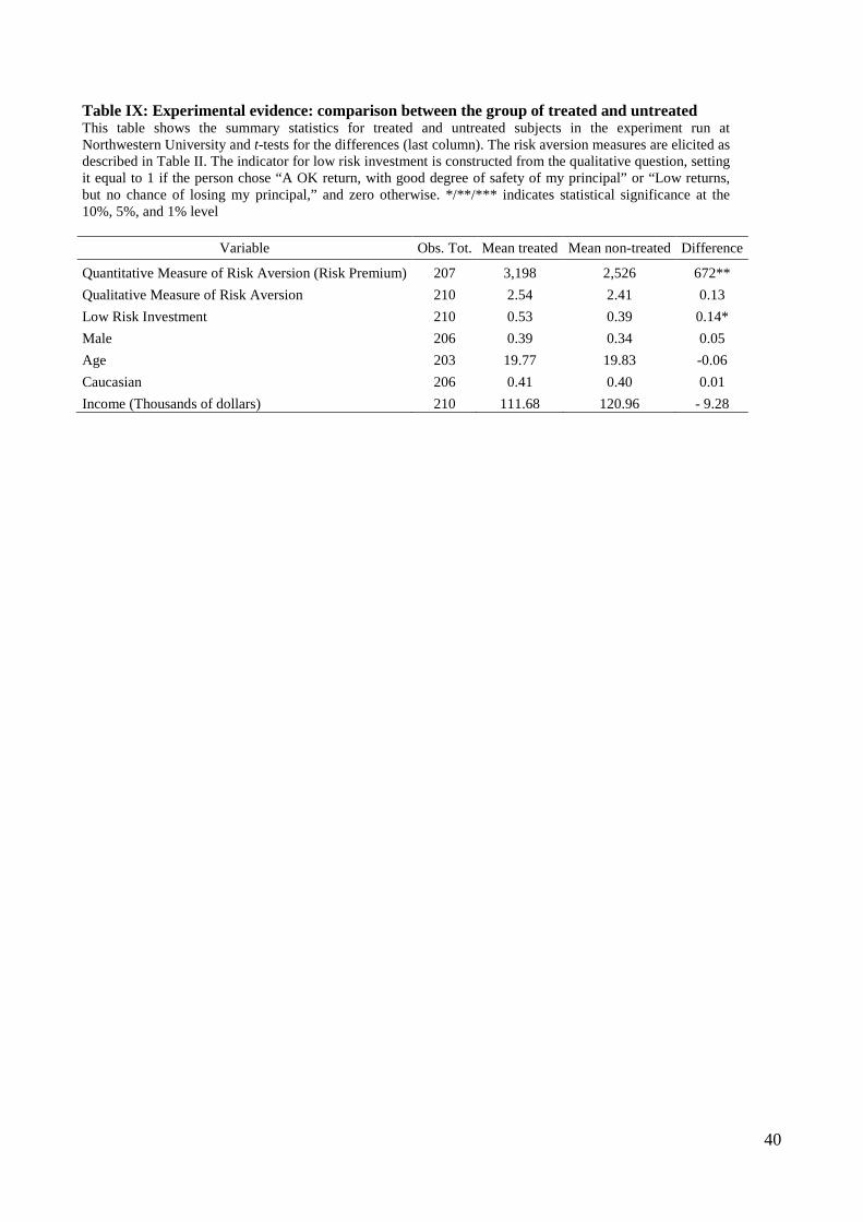
40

Table IX: Experimental evidence: comparison between the group of treated and untreated This table shows the summary statistics for treated and untreated subjects in the experiment run at Northwestern University and t-tests for the differences (last column). The risk aversion measures are elicited as described in Table II. The indicator for low risk investment is constructed from the qualitative question, setting it equal to 1 if the person chose “A OK return, with good degree of safety of my principal” or “Low returns, but no chance of losing my principal,” and zero otherwise. */**/*** indicates statistical significance at the 10%, 5%, and 1% level

Variable Obs. Tot. Mean treated Mean non-treated Difference

Quantitative Measure of Risk Aversion (Risk Premium) 207 3,198 2,526 672** Qualitative Measure of Risk Aversion 210 2.54 2.41 0.13 Low Risk Investment 210 0.53 0.39 0.14* Male 206 0.39 0.34 0.05 Age 203 19.77 19.83 -0.06 Caucasian 206 0.41 0.40 0.01 Income (Thousands of dollars) 210 111.68 120.96 - 9.28