tilburg university adjustable robust parameter design with ... · ronmental inputs, classic robust...
TRANSCRIPT

Tilburg University
Adjustable Robust Parameter Design with Unknown Distributions
Yanikoglu, I.; den Hertog, D.; Kleijnen, Jack P.C.
Publication date:2013
Link to publication
Citation for published version (APA):Yanikoglu, I., den Hertog, D., & Kleijnen, J. P. C. (2013). Adjustable Robust Parameter Design with UnknownDistributions. (CentER Discussion Paper; Vol. 2013-022). Tilburg: Econometrics.
General rightsCopyright and moral rights for the publications made accessible in the public portal are retained by the authors and/or other copyright ownersand it is a condition of accessing publications that users recognise and abide by the legal requirements associated with these rights.
- Users may download and print one copy of any publication from the public portal for the purpose of private study or research - You may not further distribute the material or use it for any profit-making activity or commercial gain - You may freely distribute the URL identifying the publication in the public portal
Take down policyIf you believe that this document breaches copyright, please contact us providing details, and we will remove access to the work immediatelyand investigate your claim.
Download date: 05. Apr. 2020
Ihsan Yaniko
No. 2013-022
ADJUSTABLE ROBUST PARAMETER DESI
WITH UNKNOWN DISTRIB
By
Ihsan Yanikoğlu, Dick den Hertog, Jack P.C. Kleijnen
March 21, 2013
ISSN 0924-7815 ISSN 2213-9532
RAMETER DESIGN WITH UNKNOWN DISTRIBUTIONS
lu, Dick den Hertog, Jack P.C. Kleijnen
Adjustable Robust Parameter Designwith Unknown Distributions
Ihsan Yanıkoglu • Dick den Hertog • Jack P.C. KleijnenCenter for Economic Research (CentER), Tilburg University, 5000 LE Tilburg, The Netherlands
[email protected] • [email protected] • [email protected]
This article presents a novel combination of robust optimization developed in mathematical programming,
and robust parameter design developed in statistical quality control. Robust parameter design uses metamod-
els estimated from experiments with both controllable and environmental inputs (factors). These experiments
may be performed with either real or simulated systems; we focus on simulation experiments. For the envi-
ronmental inputs, classic robust parameter design assumes known means and covariances, and sometimes
even a known distribution. We, however, develop a robust optimization approach that uses only experimen-
tal data, so it does not need these classic assumptions. Moreover, we develop ‘adjustable’ robust parameter
design which adjusts the values of some or all of the controllable factors after observing the values of some
or all of the environmental inputs. We also propose a new decision rule that is suitable for adjustable integer
decision variables. We illustrate our novel method through several numerical examples, which demonstrate
its effectiveness.
Key words : robust optimization; simulation optimization; robust parameter design; phi-divergence
JEL classification: C00, C15, C44, C61, C63, C67
1. Introduction
The goal of many experiments is to estimate the best solution for a given practical problem. Such
experiments may be conducted with a physical system (e.g., an airplane model in a wind tunnel) or
a mathematical model of a physical system (e.g., a computerized simulation model of an airplane or
an inventory management system). These experiments produce data on the outputs or responses for
the given inputs or factors. Output may be univariate (a single or scalar response) or multivariate
(multiple responses or a vector with responses). The number of inputs may range from a single
input to ‘many’ inputs (e.g., thousands of inputs), but we focus on practical problems with no
more than (say) twenty inputs.
Taguchi (1987)—for an update see Myers et al. (2009, pp. 483–485)—distinguishes between the
following two types of inputs: (i) Controllable or decision factors (say) dj (j = 1, . . . , k), collected in
the k-dimensional vector d = (d1, . . . , dk)T
. (ii) Environmental or noise factors (say) eg (g= 1, . . . , c),
collected in the c-dimensional vector e = (e1, . . . , ec)T
. By definition, the first type of inputs is under
the control of the users; e.g., in an inventory system, management controls the order quantity. The
second type of inputs is not controlled by the users; e.g., demand in an inventory system. Taguchi
1
Yanıkoglu, den Hertog, and Kleijnen: Adjustable Robust Parameter Design with Unknown Distributions2
emphasizes that the noise factors create variability in the outputs. Consequently, the combination
of decision factors that (say) maximizes the expected univariate output may cause the variance of
that output to be much larger than a combination that ‘nearly’ maximizes the mean output; i.e.,
a little sacrifice in expected output may save a lot of problems caused by the variability in the
output (or as the French proverb states: “the good is the enemy of the best”).
Taguchian robust parameter design (RPD) has been criticized by statisticians; see the panel
discussion reported in Nair et al. (1992). Their main critique concerns the statistical design and
analysis in the Taguchian approach; for details we refer to Taguchi (1987) and Myers et al. (2009,
pp. 483–495). An alternative RPD approach is given by Myers et al. (2009, pp. 502–506). Like Myers
et al. do, we assume that the unknown input/output (I/O) function (say) w= g(e,d) for a single
output w of the system is approximated by the following ‘incomplete’ second-order polynomial
regression metamodel:
y(e,d) =β0 +βT
d + dT
Bd +γT
e + dT
∆e + ε (1)
where y denotes the output of the regression metamodel of the simulation model with output w;
β0 the intercept; β = (β1, . . . , βk)T
the first-order effects of the decision variables d; B the k× k
symmetric matrix of second-order effects of d with on the main diagonal the ‘purely quadratic’
effects βj;j and off this diagonal half the interactions between pairs of decision factors βj;j′/2 (j 6= j′);
γ = (γ1, . . . , γc)T
the first-order effects of the environmental factors e; ∆ = (δj;g) the k× c pairwise
(two-factor) interactions between d and e; ε the residual with E(ε) = 0 if this model has no ‘lack
of fit’ (so it is a valid or adequate approximation of g(e,d)) and with constant variance σ2ε .
Myers et al. (2009) assume experiments with real systems; whereas we assume experiments
with simulation models of real systems. These simulation models may be either deterministic
(especially in engineering) or random (stochastic, possibly with discrete events). Deterministic
simulation models have noise if a parameter or input variable has a fixed but unknown value;
this is called subjective or epistemic uncertainty; see Iman and Helton (2006). Random simulation
models also have objective, aleatory or inherent uncertainty; again see Iman and Helton. We focus
on random simulation, but shall also discuss deterministic simulation. Simulation analysts use
different names for metamodels, such as response surfaces, surrogates, and emulators; see the
many references in Kleijnen (2008, p. 8). There are different types of metamodels, but the most
popular types are low-order polynomials such as (1) and Kriging (Gaussian process) models. These
polynomials are nonlinear in the inputs (e,d) but linear in the regression parameters (β0, . . . , δk;c)
so the analysis may use classic linear regression models estimated using the least squares (LS)
criterion; see Kleijnen (2008, pp. 15–72) and Myers et al. (2009, pp. 13–71). Kriging models are
Yanıkoglu, den Hertog, and Kleijnen: Adjustable Robust Parameter Design with Unknown Distributions3
more flexible so they can accurately approximate the true I/O function over bigger experimental
areas; see Kleijnen (2008, pp. 139–156).
Classic RPD assumes that the mean and variance—and sometimes even the probability
distribution—of e are known. The final parameter design may be sensitive to these assumptions.
We therefore propose a robust optimization approach that takes the distribution ambiguity into
account, and that uses historical data on the environmental inputs. The developments in robust
optimization (RO) started with Ben-Tal and Nemirovski (1998, 1999) and El-Ghaoui and Lebret
(1997). Optimization problems usually have uncertain coefficients in the objective function and
the constraints, so the “nominal” optimal solution—i.e., the optimal solution if there would be no
uncertainties—may easily violate the constraints for some realizations of the uncertain coefficients.
Therefore, it is better to find a “robust” solution, which is immune to the uncertainty in a so-
called uncertainty set. The robust reformulation of a given uncertain mathematical optimization
problem is called the robust counterpart (RC) problem. The mathematical challenge in RO is to
find computationally tractable RCs; see Ben-Tal et al. (2009).
Optimization of systems being simulated—called simulation optimization (SO)—is a popular
research topic in discrete-event simulation; see Fu (2007), and Fu and Nelson (2003). ‘Robust’ SO,
however, is hardly discussed in that literature; only recently, Angun (2011) combines Taguchi’s
worldview with response surface methodology (RSM). This RSM is a stepwise optimization heuris-
tic that in the various steps uses local first-order polynomial metamodels and in the final step uses a
local second-order polynomial metamodel (obviously, these polynomials are linear regression mod-
els). Instead of Taguchi’s various criteria, Angun (2011) uses the average value-at-risk (also known
as conditional value-at-risk). Miranda and Del Castillo (2011) perform RPD optimization through
a well-known SO method; namely, simultaneous perturbation stochastic approximation, which is
detailed in Spall (2003). More precisely, Miranda and Del Castillo’s (2011, p. 201) “objective is to
determine the operating conditions for a process so that a performance measure y is as close as pos-
sible to the desired target value and the variability around that target is minimum”. Wiedemann
(2010, p. 31) applies Taguchian RPD to an agent-based simulation, ensuring that the mean response
meets the target value and the variability around that level is sufficiently small. Some years ago,
Al-Aomar (2006) used Taguchi’s signal-to-noise ratio and a quality loss function, together with a
genetic algorithm with a scalar fitness measure that is a combination of the estimated mean and
variance. An older paper is Sanchez (2000), who used Taguchi’s worldview with a loss function that
incorporates both system’s mean and variability, and RSM; the author gave many more references.
Robust approaches are discussed—albeit briefly—not only in discrete-event simulation but also in
deterministic simulation if that simulation has uncertain environmental variables, which (by defi-
nition) are beyond management’s control. A recent example is Hu et al. (2012), who apply RO to a
Yanıkoglu, den Hertog, and Kleijnen: Adjustable Robust Parameter Design with Unknown Distributions4
climate simulation model (called ‘DICE’) with input parameters that have a multivariate Gaussian
distribution with uncertain or ‘ambiguous’ mean vector and covariance matrix. Another recent
example is Dellino et al. (2012), who investigate the well-known economic order quantity model
with an uncertain demand rate. Dellino et al. use Taguchi’s worldview, but replace his experimen-
tal designs (namely, orthogonal arrays) and metamodels (namely, low-order polynomials) by Latin
hypercube sampling and Kriging metamodels. Many more applications can be found in engineering.
For example, Chan and Ewins (2010) use Taguchi’s RPD to manage the vibrations in bladed discs.
Urval et al. (2010) use Taguchi’s RPD in powder injection moulding of microsystems’ components.
Delpiano and Sepulveda (2006) also study RPD in engineering. Vanlı and Del Castillo (2009) study
on-line RPD (ORPD) to account for control variables that are adjusted over time according to
the on-line observations of environmental factors. They assume the posterior predictive densities of
responses and environmental factors are known; moreover, they assume that the uncertain param-
eters follow a specific time series model. They propose two Bayesian approaches for ORPD. In
both approaches, controllable factors can be adjusted on-line using an expected loss function and
the on-line observations. Joseph (2003) proposes RPD with feed-forward control for measurement
systems where true values of the responses cannot be observed but estimated. Using the on-line
observable environmental factors, the author proposes a control law that periodically updates the
online measurement of the system. Dasgupta and Wu (2006) propose an on-line feedback control
mechanism that adjusts the observed output error using a controllable factor—called adjustment
factor—that is set on-line during production. All these ORPD methods assume that the mean and
variance—sometimes even the probability distribution—of environmental factors are known.
We present a methodology that is a novel combination of RPD and RO. Based on Ben-Tal et al.
(2013) and Yanıkoglu and den Hertog (2012), we use experimental data on the simulated system
to derive uncertainty sets—to be used in RO—for the unknown probability distribution of the
environmental factors. Furthermore, we also use Ben-Tal, den Hertog, and Vial (2012) to convert
associated RCs into explicit and computationally tractable optimization problems. Bingham and
Nair (2012) point out that “the noise distributions are rarely known, and the choices are often
based on convenience”. The advantage of our approach is that it uses the distribution-free structure
of RO; i.e., unlike standard approaches we do not make any assumptions about the distribution
of the environmental factors such as a Gaussian (or Normal) distribution. Moreover, we develop
adjustable RPD for those situations in which some or all of the controllable inputs have a ‘wait
and see’ character; i.e., their values can be adjusted after observing the values of some or all of
the environmental inputs. Examples are the adjustment of several controllable chemical process
parameters after observing environmental inputs such as temperature and humidity, or the adjust-
ment of the replenishment order at time t according to the realized demands in the preceding
Yanıkoglu, den Hertog, and Kleijnen: Adjustable Robust Parameter Design with Unknown Distributions5
t− 1 periods in a multistage inventory system. We develop adjustable RO for such situations, and
show that the corresponding robust counterpart problems can again be reformulated as tractable
optimization problems.
The major contributions of our research can be summarized as follows: (i) We propose a RO
methodology for a class of RPD problems where the distributional parameters are unknown
but historical data on the uncertain parameters are available. (ii) We propose adjustable robust
approach for RPD. Unlike classic adjustable RO techniques, our adjustable robust reformulations
are tractable even for nonlinear decision rules. (iii) We propose tractable RC formulations of uncer-
tain optimization problems that have quadratic terms in the uncertain parameters. Compared with
other studies in the literature, our formulations can handle more general classes of uncertainty sets,
and lead to easier tractable formulations. (iv) Last but not least, to the best of our knowledge, our
study is the first publication that introduces adjustable integer decision variables in the context of
RO, and proposes a specific decision rule for such variables.
We organize this article as follows. §2 summarizes Taguchi’s world view and the corresponding
regression model formulated in (1), and alternative RPD approaches. §3 proposes our RO approach
accounting for distribution ambiguity. §4 develops adjustable RPD. §5 presents numerical examples.
§6 summarizes our conclusions, and indicates topics for future research.
2. Robust Parameter Design
In this section, we first present the Taguchian RPD approach, and then other popular RPD
approaches. To estimate the regression parameters in (1) we need an experiment with the under-
lying system: Design of experiments (DoE) uses coded—also called standardized or scaled—values
(say) xj for the factors. So the experiment consists of (say) n combinations of the coded factors x,
which correspond with d and e in (1). Coding is further discussed in Kleijnen (2008, p. 29) and
Myers et al. (2009, p. 78).
We reformulate the Taguchian model (1) as the following linear regression model :
y= ζT
x + ε (2)
with the `-dimensional vector of regression parameters or coefficients ζ = (β0, . . . , δk;c)T
and the
corresponding vector of regression explanatory variables x defined in the obvious way; e.g., the
explanatory variable corresponding with the interaction effect β1;2 is d1d2. Then (2) leads to the
LS estimator:
ζ = (XT
X)−1
XT
y (3)
where X is the n × ` matrix of explanatory variables with n denoting the number of scenarios
(combinations of control and environmental factors) determined by the DoE that are actually
Yanıkoglu, den Hertog, and Kleijnen: Adjustable Robust Parameter Design with Unknown Distributions6
observed (in a real or simulated system); y is the vector with the n observed outputs. The covariance
matrix of the estimator (3) is
Cov(ζ) = σ2ε (X
T
X)−1
(4)
where σ2ε was defined in (1). Hence, the variance σ2
ε may be estimated by the mean squared
residuals:
σ2ε =
(y−y)T
(y−y)
n− `(5)
where y = Xζ; see (2) and (3).
We denote the expected values of the environmental factors through E(e) =µe. We allow depen-
dence between the environmental factors so the covariance matrix is Cov(e) = Ωe. Analogous to
Myers et al. (2009, pp. 504–506), we derive that the metamodel (1) implies that the regression
predictor for the mean E(y) is
Ee[y(e,d)] =β0 +βT
d + dT
Bd +γT
µe + dT
∆µe (6)
and the regression predictor for the variance Var(y) is
Vare[y(e,d)] = (γT
+ d∆)Ωe(γ+ ∆T
d) +σ2ε (7)
where (γ+∆Td) = (∂y/∂e1, . . . , ∂y/∂ec)
Tis the gradient with respect to the environmental factors.
Obviously, the larger the gradient’s elements are, the larger the variance of the predicted output
is. Furthermore, if ∆ = 0 (no control-by-noise interactions), then Var(y) cannot be controlled
through the decision variables d. Note the difference between the predicted variance, Var(y), and
the variance of the predictor, Var(y) with y= xTζ. Obviously, the mean vector and the covariance
matrix completely define a multi-variate Gaussian distribution.
Taguchi focuses his analysis on the signal-to-noise ratios (SNRs), which depend on
E(y)/√
Var(y) (the standard deviation√
Var(y) has the same scale as the mean E(y)); see Myers
et al. (2009, pp. 486–488). The precise definitions of these SNRs vary with the following goals of
RPD: (i) ‘The smaller, the better’: minimize the response. (ii) ‘The larger, the better’: maximize
the response. (iii) ‘The target is best’: realize a target value (say) T for the response.
We do not further dwell on Taguchi’s SNRs, because we think there are better formulations of
the various goals of RPD; Myers et al. (2009, pp. 488–495) also question the utility of SNRs. We
use the following optimization problem formulation, also formulated by Myers et al. (2009, p. 506):
mind
Vare[y(e,d)] s.t. Ee[y(e,d)]≤ T. (8)
We may also consider the optimization problem given by Dellino et al. (2012); namely,
mind
Ee[y(e,d)] s.t. Vare[y(e,d)]≤ T, (9)
Yanıkoglu, den Hertog, and Kleijnen: Adjustable Robust Parameter Design with Unknown Distributions7
or the following variant:
mind
Ee[(y(e,d)−T )2]. (10)
Remark 1 The optimal ‘coded’ controllable factors d∗—that minimize the process mean or vari-
ance in (8), (9) or (10)—must lie in −1≤ d≤ 1, where 1 denotes the all ones vector. Otherwise,
the simulation or physical experiment must be rerun with a larger experimental region for the orig-
inal (non-coded) input factors to obtain a new response model y(e,d) satisfying the associated
requirement for the given RPD problem.
In the rest of this paper we focus on (9), since (8) and (10) can be treated analogously.
3. Robust Optimization with Unknown Distributions
In this section, we derive the robust reformulations of the class of optimization problems presented
in §2. We assume that data on the environmental factors e is available or can be obtained via
simulation.
3.1. Uncertainty Sets
Instead of relying on the normal distribution, RO derives an uncertainty set for the unknown
density function of the noise factors. There are several RO approaches, but we follow Ben-Tal et
al. (2013) and Yanıkoglu and den Hertog (2012), who develop RO accounting for historical data on
the noise factors. They do not use a specific distribution to this data; instead, they use the more
general concept of phi-divergence—as follows.
Given N historical observations on the noise factors e, we construct m cells such that the number
of observations oi in cell i (i= 1, . . . ,m) is at least five:∑m
i=1oi =N such that ∀i : oi ≥ 5.
The historical data on e give the frequencies q = [q1, . . . , qm]T
, where qi is the observed frequency
in cell i so
qi =oiN.
The phi-divergence measure is
Iφ(p,q) =m∑i=1
qiφ
(piqi
)where φ(.) satisfy certain mathematical requirements such as φ (1) = 0, φ (a/0) := a lim
t→∞φ(t)/t for
a> 0, and φ (0/0) = 0; for details on phi-divergence we refer to Pardo (2006). It can be proven that
the test statistic2N
φ′′(1)Iφ(p,q)
Yanıkoglu, den Hertog, and Kleijnen: Adjustable Robust Parameter Design with Unknown Distributions8
is asymptotically distributed as a chi-squared random variable with (m−1) degrees of freedom. So
an asymptotic (1−α)-confidence set for p is
Iφ(p,q)≤ ρ with ρ= ρ(N,m,α) =φ′′(1)
2Nχ2m−1;1−α. (11)
Using (11), Ben-Tal et al. (2013) derive the following uncertainty set U for the unknown probability
vector p:
U = p∈Rm|p≥ 0,m∑i=1
pi = 1, Iφ(p,q)≤ ρ. (12)
Table 1 Phi-Divergence Examples
Divergence φ(t), t > 0 Iφ(p,q) φ∗(s)
Kullback-Leibler t log t∑i
pi log
(pi
qi
)es−1
Burg entropy − log t∑i
qi log
(pi
qi
)−1− log(−s), s≤ 0
χ2-distance 1
t(t− 1)2
∑i
(pi− qi)2
pi2− 2
√1− s, s≤ 1
Pearson χ2-distance (t− 1)2∑i
(pi− qi)2
qi
s+ s2/4, s≥−2−1, s <−2
Hellinger distance (1−√t)2
∑i
(√pi−√qi)
2 s
1−s , s≤ 1
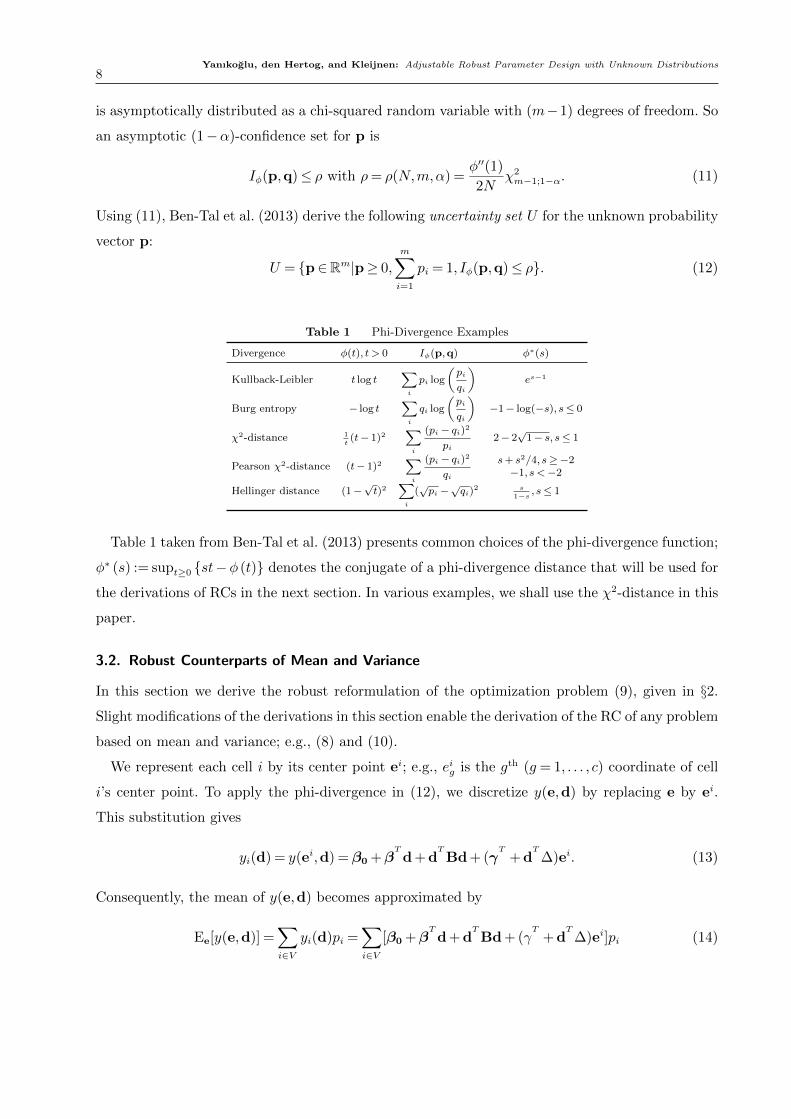
Table 1 taken from Ben-Tal et al. (2013) presents common choices of the phi-divergence function;
φ∗ (s) := supt≥0 st−φ (t) denotes the conjugate of a phi-divergence distance that will be used for
the derivations of RCs in the next section. In various examples, we shall use the χ2-distance in this
paper.
3.2. Robust Counterparts of Mean and Variance
In this section we derive the robust reformulation of the optimization problem (9), given in §2.
Slight modifications of the derivations in this section enable the derivation of the RC of any problem
based on mean and variance; e.g., (8) and (10).
We represent each cell i by its center point ei; e.g., eig is the gth (g = 1, . . . , c) coordinate of cell
i’s center point. To apply the phi-divergence in (12), we discretize y(e,d) by replacing e by ei.
This substitution gives
yi(d) = y(ei,d) =β0 +βT
d + dT
Bd + (γT
+ dT
∆)ei. (13)
Consequently, the mean of y(e,d) becomes approximated by
Ee[y(e,d)] =∑i∈V
yi(d)pi =∑i∈V
[β0 +βT
d + dT
Bd + (γT
+ dT
∆)ei]pi (14)
Yanıkoglu, den Hertog, and Kleijnen: Adjustable Robust Parameter Design with Unknown Distributions9
where pi denotes the probability of e falling into cell i. Note that p is in the uncertainty set U
given by (12) and the empirical estimate q of p is obtained using the data on e; see §3.1. If we
define
ψi(d) := (γT
+ dT
∆)ei, (15)
then the variance of y(e,d) becomes approximated by
Vare[y(e,d)] =∑i∈V
ψi(d)2pi−
[∑i∈V
ψi(d)pi
]2. (16)
Eventually, the robust reformulation of (9) is the following semi-infinite optimization problem:
(SI1) mind
maxp∈U
∑i∈V
[β0 +βT
d + dT
Bd + (γT
+ dT
∆)ei]pi
s.t.∑i∈V
ψi(d)2pi−
[∑i∈V
ψi(d)pi
]2≤ T ∀p∈U, (17)
where U = p ∈Rm|p≥ 0,∑m
i=1 pi = 1, Iφ(p,q)≤ ρ. (SI1) is a difficult optimization problem that
has infinitely many constraints (see ∀p ∈ U), and includes quadratic terms in p. Ben-Tal et al.
(2009, p. 382) propose a tractable RC of a linear optimization problem with uncertain parameters
that appear quadratically, and an ellipsoidal uncertainty. The resulting formulation is a semidefinite
programming (SDP) problem; see also Remark 2 below. The following theorem provides tractable
RC reformulations of (SI1) for more general ‘phi-divergence’ uncertainty sets.
Theorem 1 The vector d solves (SI1) if and only if d,λ,η, and z solve the following RC problem:
(RC1) mind,λ,η,z
β0 +βT
d + dT
Bd +λ1 + ρη1 + η1∑i∈V
qiφ∗(ψi(d)−λ1
η1
)
s.t. λ2 + ρη2 + η2∑i∈V
qiφ∗
((ψi(d) + z)
2−λ2
η2
)≤ T (18)
η1, η2 ≥ 0
where ρ is given by (11), φ∗ (s) := supt≥0 st−φ (t) denotes the conjugate of φ(.), V = 1, ...,m
is the set of cell indices in the uncertainty set U , qi is the data frequency in cell i ∈ V using the
historical data on e, and λ, η, and z are additional variables.
Proof. Using Yanıkoglu and den Hertog (2012, Theorem 1), we can easily derive the explicit RC of
the objective function of (SI1) that is linear in p∈U . Next we consider the ‘more difficult’ variance
constraint (17), which is quadratic in p. In the following parts of the proof we use Ben-Tal, den
Yanıkoglu, den Hertog, and Kleijnen: Adjustable Robust Parameter Design with Unknown Distributions10
Hertog, and Vial (2012) to account for the nonlinear uncertainty in the constraint. Using a linear
transformation, we reformulate (17) as
maxa∈U
g(a)≤ T, (19)
where U := a : a = Ap,p∈U, AT
= [ψ2(d),ψ(d)] and g(a) = a1−a22. Using the indicator function
δ(a|U) :=
0, a∈ U
+∞, elsewhere,
we reformulate (19) as
maxa∈R2g(a)− δ(a|U) ≤ T. (20)
The Fenchel dual of (20)—for details see Rockafellar (1970, pp. 327–341)— is equivalent to
minv∈Rnδ∗(v|U)− g∗(v) ≤ T (21)
where v denotes the dual variable, and δ∗(v|U) := supp∈UaTv|a = Ap and g∗(v) := infa∈R2aTv−
g(a) denote the convex and concave conjugates of the functions δ and g, respectively. Going from
(20) to (21) is justified since the intersection of the relative interiors of the domains of g(.) and
δ(.|U) is non-empty, since a = Aq is always in the relative interiors of both domains. Moreover it
is easy to show that δ∗(v|U) = δ∗(ATv|U). Then we delete the minimization in (21) because the
constraint has the ≤ operator, and the RC reformulation of (17) becomes
δ∗(AT
v|U)− g∗(v)≤ T.
Now we derive the complete formulas of the conjugate functions δ∗ and g∗. If vT
= [w,z], then the
concave conjugate of g is equivalent to
g∗(v) = infa∈R2a1w+ a2z− g(a)=
−z2/4, w= 1−∞, elsewhere.
Using Theorem 1 in Yanıkoglu and den Hertog (2012) once more, the convex conjugate of δ is
equivalent to
δ∗(AT
v|U) = infλ,η2≥0
ρη2 +λ+ η2
∑i∈V
qiφ∗(ψ2i (d) +ψi(d)z−λ
η2
).
Thus the RC reformulation of (17) becomes
λ+ ρη2 + η2∑i∈V
qiφ∗(ψ2i (d) +ψi(d)z−λ
η2
)+z2
4≤ T,η2 ≥ 0. (22)
Substituting λ2 = λ+ z2/4 into (22) gives the final RC reformulation (RC1)
Yanıkoglu, den Hertog, and Kleijnen: Adjustable Robust Parameter Design with Unknown Distributions11
Remark 2 An ellipsoidal uncertainty set is a special case of the phi-divergence uncertainty set (12)
when the Pearson chi-squared distance is used as the phi-divergence. Moreover, we can reformulate
(RC1) as a second order cone problem (SOCP) for the associated distance measure. Notice that
SOCP is an ‘easier’ formulation of the problem compared with the SDP by Ben-Tal et al. (2009).
Remark 3 Ben-Tal et al. (2012) also propose an RC for the variance uncertainty, however the
associated RC introduces additional non-convexity. We overcome this difficulty by using the substi-
tution λ2 = λ+ z2/4 in the proof of Theorem 1.
We now discuss the ‘general’ computational tractability of (RC1). First, φ∗(h(d, λ2, z)) is convex,
since the convex conjugate φ∗ (s) := supt≥0 st−φ (t) is non-decreasing in s, and h(d, λ2, z) =
(ψi(d) + z)2 − λ2 is convex in d, z, and λ2. It is easy to show that η2φ∗(·/η2) is convex, since the
perspective of a convex function is always convex. Eventually, the convexity of the perspective
implies that (18) is convex. On the other hand, the objective function of (RC1) is not necessarily
convex, since y is non-convex in d unless B is a positive semidefinite (PSD) matrix. Nevertheless,
(RC1) does not introduce additional non-convexity into the general optimization problem (9).
3.3. Alternative Metamodels and Risk Measures
In this subsection, we focus on extensions of our method. §3.3.1 presents a generalization of our
method for other metamodels besides (2), and §3.3.2 presents an extension of our method to SNRs.
Finally, §3.3.3 shows how to apply our method to tail-risk measures.
3.3.1. Alternative Metamodels In this paper we focus on the low-order polynomial (1),
since most of the literature and real-life applications use low-order polynomials to approximate the
I/O function of the underlying simulation or physical experiment. However, our methodology can
also be used to other metamodel types such as higher-order polynomials, Kriging, and radial basis
functions. More precisely, consider
y(d,e) = f(d) +ψ(d,e)
where f(d) is the part that affects only the mean of the response (e.g., it is f(d) = β0 +βTd+d
TBd
in (1)), and ψ(d,e) is the part that affects the response variance (e.g., it is ψ(d,e) = γTe + d
T∆e
in (1)). We then reformulate the RC in Theorem 1 as
mind,λ,η,z
f(d) +λ1 + ρη1 + η1∑i∈V
qiφ∗(ψi(d)−λ1
η1
)
s.t. λ2 + ρη2 + η2∑i∈V
qiφ∗
((ψi(d) + z)
2−λ2
η2
)≤ T
η1, η2 ≥ 0.
Yanıkoglu, den Hertog, and Kleijnen: Adjustable Robust Parameter Design with Unknown Distributions12
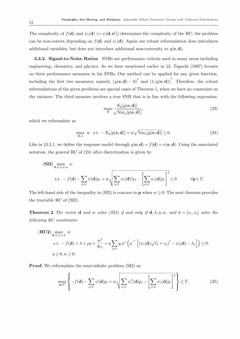
The complexity of f(d) and ψi(d) (=ψ(d,ei)) determines the complexity of the RC; the problem
can be non-convex depending on f(d) and ψi(d). Again our robust reformulation does introduces
additional variables, but does not introduce additional non-convexity to y(e,d).
3.3.2. Signal-to-Noise Ratios SNRs are performance criteria used in many areas including
engineering, chemistry, and physics. As we have mentioned earlier in §2, Taguchi (1987) focuses
on three performance measures in his SNRs. Our method can be applied for any given function,
including the first two measures; namely, (y(e,d) − 0)2
and (1/y(e,d))2
. Therefore, the robust
reformulations of the given problems are special cases of Theorem 1, when we have no constraint on
the variance. The third measure involves a true SNR that is in line with the following expression:
maxd
Ee[y(e,d)]√Vare[y(e,d)]
, (23)
which we reformulate as
maxd,w
w s.t. −Ee[y(e,d)] +w√
Vare[y(e,d)]≤ 0. (24)
Like in §3.3.1, we define the response model through y(e,d) = f(d) +ψ(e,d). Using the associated
notation, the general RC of (24) after discretization is given by
(SI2) maxd,λ,η,w,v
w
s.t. − f(d)−∑i∈V
ψ(d)pi +w
√√√√∑i∈V
ψi(d)2pi−
[∑i∈V
ψi(d)pi
]2≤ 0 ∀p∈U.
The left-hand side of the inequality in (SI2) is concave in p when w≥ 0. The next theorem provides
the tractable RC of (SI2).
Theorem 2 The vector d and w solve (SI2) if and only if d, λ, η,w, and v = [v1, v2] solve the
following RC constraints:
(RC2) maxd,λ,η,w,v
w
s.t. − f(d) +λ+ ρη+w2
4v1+ η
∑i∈V
qiφ∗(η−1[(ψi(d)
√v1 + v2)
2
−ψi(d)−λ1
])≤ 0,
η≥ 0,w≥ 0.
Proof. We reformulate the semi-infinite problem (SI2) as
maxp∈U
−f(d)−∑i∈V
ψ(d)pi +w
√√√√∑i∈V
ψ2
i (d)pi−
[∑i∈V
ψi(d)pi
]2≤ T. (25)
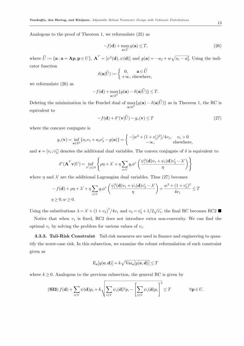
Yanıkoglu, den Hertog, and Kleijnen: Adjustable Robust Parameter Design with Unknown Distributions13
Analogous to the proof of Theorem 1, we reformulate (25) as
−f(d) + maxa∈U
g(a)≤ T, (26)
where U := a : a = Ap,p ∈ U, AT
= [ψ2(d),ψ(d)] and g(a) =−a2 +w√a1− a22. Using the indi-
cator function
δ(a|U) :=
0, a∈ U
+∞, elsewhere,
we reformulate (26) as
−f(d) + maxa∈R2g(a)− δ(a|U) ≤ T.
Deleting the minimization in the Fenchel dual of maxa∈R2g(a)− δ(a|U) as in Theorem 1, the RC is
equivalent to
−f(d) + δ∗(v|U)− g∗(v)≤ T (27)
where the concave conjugate is
g∗(v) = infa∈R2a1v1 + a2v
′2− g(a)=
−[w2 + (1 + v′2)
2]/4v1, v1 > 0−∞, elsewhere,
and v = [v1;v′2] denotes the additional dual variables. The convex conjugate of δ is equivalent to
δ∗(AT
v|U) = infλ′,η≥0
ρη+λ′+ η
∑i∈V
qiφ∗(ψ2i (d)v1 +ψi(d)v′2−λ′
η
)where η and λ′ are the additional Lagrangian dual variables. Thus (27) becomes
− f(d) + ρη+λ′+ η∑i∈V
qiφ∗(ψ2i (d)v1 +ψi(d)v′2−λ′
η
)+w2 + (1 + v′2)
2
4v1≤ T
η≥ 0,w≥ 0.
Using the substitutions λ= λ′+ (1 + v2)2/4v1 and v2 = v′2 + 1/2
√v1, the final RC becomes RC2
Notice that when v1 is fixed, RC2 does not introduce extra non-convexity. We can find the
optimal v1 by solving the problem for various values of v1.
3.3.3. Tail-Risk Constraint Tail-risk measures are used in finance and engineering to quan-
tify the worst-case risk. In this subsection, we examine the robust reformulation of such constraint
given as
Ee[y(e,d)] + k√
Vare[y(e,d)]≤ T
where k≥ 0. Analogous to the previous subsection, the general RC is given by
(SI3) f(d) +∑i∈V
ψ(d)pi + k
√√√√∑i∈V
ψi(d)2pi−
[∑i∈V
ψi(d)pi
]2≤ T ∀p∈U.
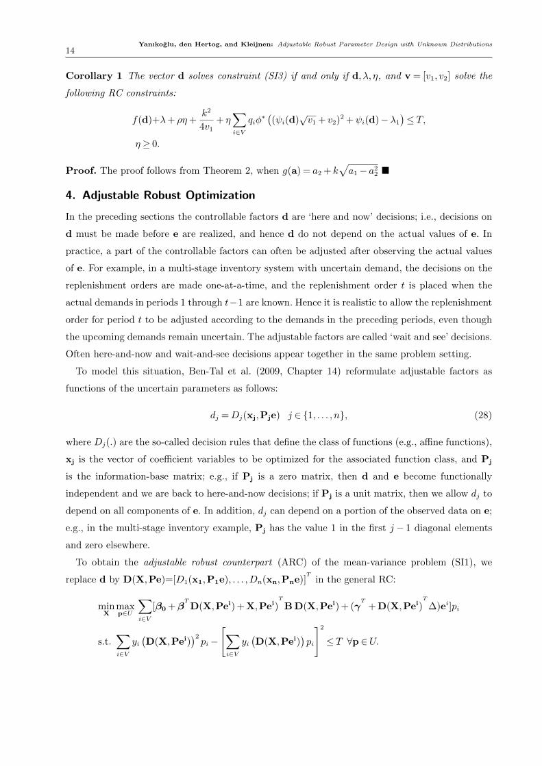
Yanıkoglu, den Hertog, and Kleijnen: Adjustable Robust Parameter Design with Unknown Distributions14
Corollary 1 The vector d solves constraint (SI3) if and only if d, λ, η, and v = [v1, v2] solve the
following RC constraints:
f(d)+λ+ ρη+k2
4v1+ η
∑i∈V
qiφ∗ ((ψi(d)
√v1 + v2)
2 +ψi(d)−λ1
)≤ T,
η≥ 0.
Proof. The proof follows from Theorem 2, when g(a) = a2 + k√a1− a22
4. Adjustable Robust Optimization
In the preceding sections the controllable factors d are ‘here and now’ decisions; i.e., decisions on
d must be made before e are realized, and hence d do not depend on the actual values of e. In
practice, a part of the controllable factors can often be adjusted after observing the actual values
of e. For example, in a multi-stage inventory system with uncertain demand, the decisions on the
replenishment orders are made one-at-a-time, and the replenishment order t is placed when the
actual demands in periods 1 through t−1 are known. Hence it is realistic to allow the replenishment
order for period t to be adjusted according to the demands in the preceding periods, even though
the upcoming demands remain uncertain. The adjustable factors are called ‘wait and see’ decisions.
Often here-and-now and wait-and-see decisions appear together in the same problem setting.
To model this situation, Ben-Tal et al. (2009, Chapter 14) reformulate adjustable factors as
functions of the uncertain parameters as follows:
dj =Dj(xj,Pje) j ∈ 1, . . . , n, (28)
where Dj(.) are the so-called decision rules that define the class of functions (e.g., affine functions),
xj is the vector of coefficient variables to be optimized for the associated function class, and Pj
is the information-base matrix; e.g., if Pj is a zero matrix, then d and e become functionally
independent and we are back to here-and-now decisions; if Pj is a unit matrix, then we allow dj to
depend on all components of e. In addition, dj can depend on a portion of the observed data on e;
e.g., in the multi-stage inventory example, Pj has the value 1 in the first j − 1 diagonal elements
and zero elsewhere.
To obtain the adjustable robust counterpart (ARC) of the mean-variance problem (SI1), we
replace d by D(X,Pe)=[D1(x1,P1e), . . . ,Dn(xn,Pne)]T
in the general RC:
minX
maxp∈U
∑i∈V
[β0 +βT
D(X,Pei) + X,Pei)T
B D(X,Pei) + (γT
+ D(X,Pei)T
∆)ei]pi
s.t.∑i∈V
yi(D(X,Pei)
)2pi−
[∑i∈V
yi(D(X,Pei)
)pi
]2≤ T ∀p∈U.
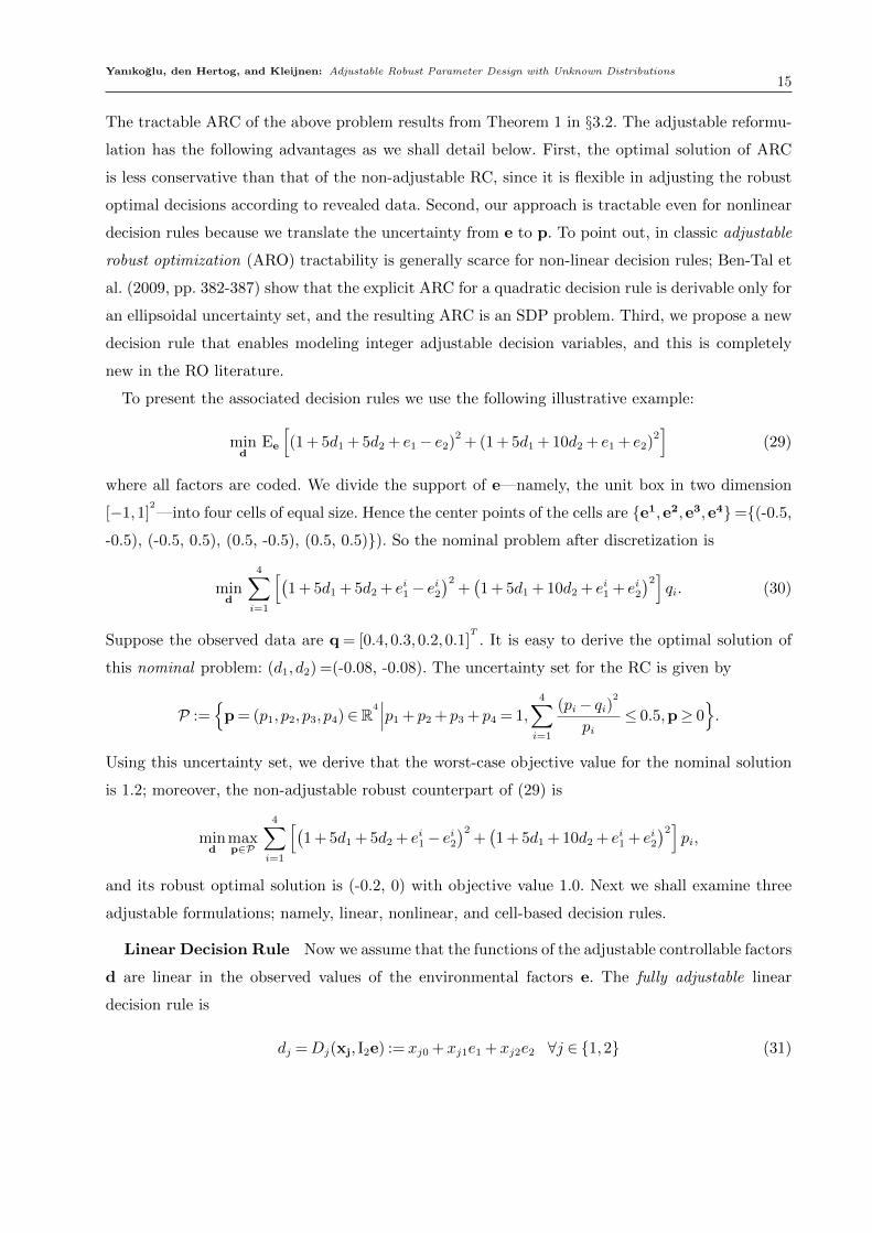
Yanıkoglu, den Hertog, and Kleijnen: Adjustable Robust Parameter Design with Unknown Distributions15
The tractable ARC of the above problem results from Theorem 1 in §3.2. The adjustable reformu-
lation has the following advantages as we shall detail below. First, the optimal solution of ARC
is less conservative than that of the non-adjustable RC, since it is flexible in adjusting the robust
optimal decisions according to revealed data. Second, our approach is tractable even for nonlinear
decision rules because we translate the uncertainty from e to p. To point out, in classic adjustable
robust optimization (ARO) tractability is generally scarce for non-linear decision rules; Ben-Tal et
al. (2009, pp. 382-387) show that the explicit ARC for a quadratic decision rule is derivable only for
an ellipsoidal uncertainty set, and the resulting ARC is an SDP problem. Third, we propose a new
decision rule that enables modeling integer adjustable decision variables, and this is completely
new in the RO literature.
To present the associated decision rules we use the following illustrative example:
mind
Ee
[(1 + 5d1 + 5d2 + e1− e2)2 + (1 + 5d1 + 10d2 + e1 + e2)
2]
(29)
where all factors are coded. We divide the support of e—namely, the unit box in two dimension
[−1,1]2—into four cells of equal size. Hence the center points of the cells are e1,e2,e3,e4=(-0.5,
-0.5), (-0.5, 0.5), (0.5, -0.5), (0.5, 0.5)). So the nominal problem after discretization is
mind
4∑i=1
[(1 + 5d1 + 5d2 + ei1− ei2
)2+(1 + 5d1 + 10d2 + ei1 + ei2
)2]qi. (30)
Suppose the observed data are q = [0.4,0.3,0.2,0.1]T
. It is easy to derive the optimal solution of
this nominal problem: (d1, d2) =(-0.08, -0.08). The uncertainty set for the RC is given by
P :=
p = (p1, p2, p3, p4)∈R4∣∣∣p1 + p2 + p3 + p4 = 1,
4∑i=1
(pi− qi)2
pi≤ 0.5,p≥ 0
.
Using this uncertainty set, we derive that the worst-case objective value for the nominal solution
is 1.2; moreover, the non-adjustable robust counterpart of (29) is
mind
maxp∈P
4∑i=1
[(1 + 5d1 + 5d2 + ei1− ei2
)2+(1 + 5d1 + 10d2 + ei1 + ei2
)2]pi,
and its robust optimal solution is (-0.2, 0) with objective value 1.0. Next we shall examine three
adjustable formulations; namely, linear, nonlinear, and cell-based decision rules.
Linear Decision Rule Now we assume that the functions of the adjustable controllable factors
d are linear in the observed values of the environmental factors e. The fully adjustable linear
decision rule is
dj =Dj(xj, I2e) := xj0 +xj1e1 +xj2e2 ∀j ∈ 1,2 (31)
Yanıkoglu, den Hertog, and Kleijnen: Adjustable Robust Parameter Design with Unknown Distributions16
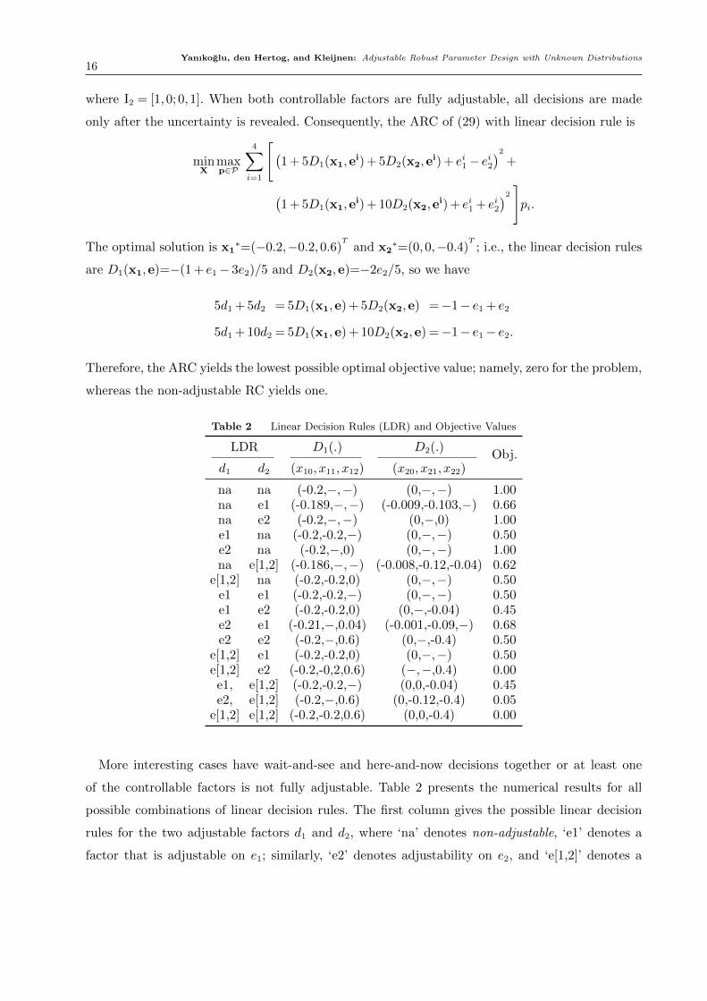
where I2 = [1,0; 0,1]. When both controllable factors are fully adjustable, all decisions are made
only after the uncertainty is revealed. Consequently, the ARC of (29) with linear decision rule is
minX
maxp∈P
4∑i=1
[(1 + 5D1(x1,e
i) + 5D2(x2,ei) + ei1− ei2
)2+
(1 + 5D1(x1,e
i) + 10D2(x2,ei) + ei1 + ei2
)2 ]pi.
The optimal solution is x1∗=(−0.2,−0.2,0.6)
Tand x2
∗=(0,0,−0.4)T
; i.e., the linear decision rules
are D1(x1,e)=−(1 + e1− 3e2)/5 and D2(x2,e)=−2e2/5, so we have
5d1 + 5d2 = 5D1(x1,e) + 5D2(x2,e) =−1− e1 + e2
5d1 + 10d2 = 5D1(x1,e) + 10D2(x2,e) =−1− e1− e2.
Therefore, the ARC yields the lowest possible optimal objective value; namely, zero for the problem,
whereas the non-adjustable RC yields one.
Table 2 Linear Decision Rules (LDR) and Objective Values
LDR D1(.) D2(.) Obj.d1 d2 (x10, x11, x12) (x20, x21, x22)
na na (-0.2,−,−) (0,−,−) 1.00na e1 (-0.189,−,−) (-0.009,-0.103,−) 0.66na e2 (-0.2,−,−) (0,−,0) 1.00e1 na (-0.2,-0.2,−) (0,−,−) 0.50e2 na (-0.2,−,0) (0,−,−) 1.00na e[1,2] (-0.186,−,−) (-0.008,-0.12,-0.04) 0.62
e[1,2] na (-0.2,-0.2,0) (0,−,−) 0.50e1 e1 (-0.2,-0.2,−) (0,−,−) 0.50e1 e2 (-0.2,-0.2,0) (0,−,-0.04) 0.45e2 e1 (-0.21,−,0.04) (-0.001,-0.09,−) 0.68e2 e2 (-0.2,−,0.6) (0,−,-0.4) 0.50
e[1,2] e1 (-0.2,-0.2,0) (0,−,−) 0.50e[1,2] e2 (-0.2,-0,2,0.6) (−,−,0.4) 0.00e1, e[1,2] (-0.2,-0.2,−) (0,0,-0.04) 0.45e2, e[1,2] (-0.2,−,0.6) (0,-0.12,-0.4) 0.05
e[1,2] e[1,2] (-0.2,-0.2,0.6) (0,0,-0.4) 0.00
More interesting cases have wait-and-see and here-and-now decisions together or at least one
of the controllable factors is not fully adjustable. Table 2 presents the numerical results for all
possible combinations of linear decision rules. The first column gives the possible linear decision
rules for the two adjustable factors d1 and d2, where ‘na’ denotes non-adjustable, ‘e1’ denotes a
factor that is adjustable on e1; similarly, ‘e2’ denotes adjustability on e2, and ‘e[1,2]’ denotes a
Yanıkoglu, den Hertog, and Kleijnen: Adjustable Robust Parameter Design with Unknown Distributions17
fully adjustable factor. The second and third columns are the optimal coefficients (variables) x1
and x2 of the decision rules D1(.) and D2(.), where (−) denotes a variable that vanishes in the
associated decision rule. The final column (Obj.) presents the robust optimal objective value for
the associated decision rule. Altogether, the numerical results show that when one of the factors
is non-adjustable and the other is adjustable on e2—see row (na, e2) or (e2, na) in Table 2—the
optimal objective value of the ARC is the same as that of the non-adjustable RC. In all other cases
the optimal objective value of the non-adjustable RC improves with at least 32% (see row (e2,
e1)) for the ARC, and the highest improvement (100%) is attained when the first factor is fully
adjustable and the second one is non-adjustable; see row (e[1,2], e2). Another interesting outcome
is that introducing an adjustable factor into the problem may change the optimal decision for the
non-adjustable factor; i.e., an optimal here-and-now factor can have different values in the ARC
and RC. For example, if d1 is adjustable on e1 and d2 is non-adjustable, then the optimal d2 is
-0.189 in the ARC, but it is -0.2 in the RC; see (na, na) and (na, e1).
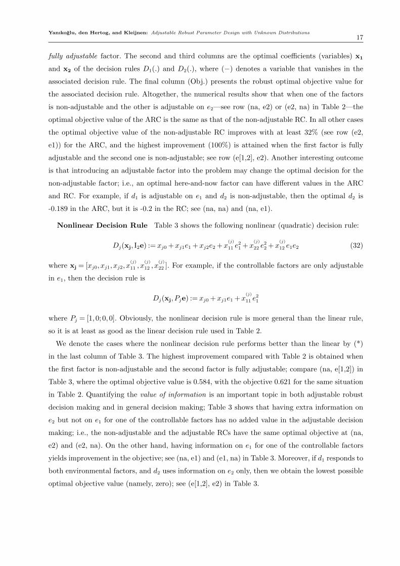
Nonlinear Decision Rule Table 3 shows the following nonlinear (quadratic) decision rule:
Dj(xj, I2e) := xj0 +xj1e1 +xj2e2 +x(j)
11 e21 +x
(j)
22 e22 +x
(j)
12 e1e2 (32)
where xj = [xj0, xj1, xj2, x(j)
11 , x(j)
12 , x(j)
22 ]. For example, if the controllable factors are only adjustable
in e1, then the decision rule is
Dj(xj, Pje) := xj0 +xj1e1 +x(j)
11 e21
where Pj = [1,0; 0,0]. Obviously, the nonlinear decision rule is more general than the linear rule,
so it is at least as good as the linear decision rule used in Table 2.
We denote the cases where the nonlinear decision rule performs better than the linear by (*)
in the last column of Table 3. The highest improvement compared with Table 2 is obtained when
the first factor is non-adjustable and the second factor is fully adjustable; compare (na, e[1,2]) in
Table 3, where the optimal objective value is 0.584, with the objective 0.621 for the same situation
in Table 2. Quantifying the value of information is an important topic in both adjustable robust
decision making and in general decision making; Table 3 shows that having extra information on
e2 but not on e1 for one of the controllable factors has no added value in the adjustable decision
making; i.e., the non-adjustable and the adjustable RCs have the same optimal objective at (na,
e2) and (e2, na). On the other hand, having information on e1 for one of the controllable factors
yields improvement in the objective; see (na, e1) and (e1, na) in Table 3. Moreover, if d1 responds to
both environmental factors, and d2 uses information on e2 only, then we obtain the lowest possible
optimal objective value (namely, zero); see (e[1,2], e2) in Table 3.
Yanıkoglu, den Hertog, and Kleijnen: Adjustable Robust Parameter Design with Unknown Distributions18
Table 3 Nonlinear Decision Rules (NDR) and Objective Values
NDR D1(.) D2(.) Obj.d1 d2 (x10, x11, x12, x
(1)11 , x
(1)22 , x
(1)12 ) (x20, x21, x22, x
(2)11 , x
(2)22 , x
(2)12 )
na na (-0.2,-,-,-,-,-) (0,-,-,-,-,-) 1.00na e1 (-0.196,-,-,-,-,-) (0.014,0.093,-,-0.079,-,-) 0.65∗
na e2 (-0.2,-,-,-,-,-) (-0.33,-,0,-,1.33,-) 1.00e1 na (-0.195,-0.2,-,-0.02,-,-) (0,-,-,-,-,-) 0.50e2 na (-0.192,-,0,-,-,-) (-,-0.03,-,-,-,-) 1.00na e[1,2] (-0.188,-,-,-,-,-) (0.062,-0.106,-0.053,-0.244,0.015,0.05) 0.58∗
e[1,2] na (-0.178,-0.2,0,-0.044,-0.044,0) (0,-,-,-,-,-) 0.50e1 e1 (-0.213,-0.2,-,0.05,-,-) (-0.002,0,-,0.008,-,-) 0.50e1 e2 (-0.533,-0.2,-,1.33,-,-) (-0.005,-,-0.04,-,0.02,-) 0.45e2 e1 (-0.19,-,0.044,-,-0.047,-) (-0.045,-0.063,-,0.197,-,-) 0.65∗
e2 e2 (-0.223,-,0.6,-,0.094,-) (-0.002,-,-0.4,-0.008,-) 0.50e[1,2] e1 (-0.186,-0.2,0,-0.028,0.028,0) (-0.006,-,-,0.023,-,-) 0.50e[1,2] e2 (-0.253,-0.2,0.6,0.107,0.107,0) (-0.002,-,-0.4,-,0.008,-) 0.00
e1 e[1,2] (-0.146,-0.199,-,-0.214,-,-) (-0.052,-0.003,-0.047,0.148,0.057,-0.001) 0.44∗
e2 e[1,2] (-0.233,0,0.6,-,0.133,0) (-0.151,-0.12,-0.4,0.105,0.5,-) 0.05e[1,2] e[1,2] (-0.214,-0.2,0.6,0.028,0.028,0) (0.013,0,-0.4,-0.066,0.014,0) 0.00
(∗) denotes an improved optimal objective value compared with that in Table 2
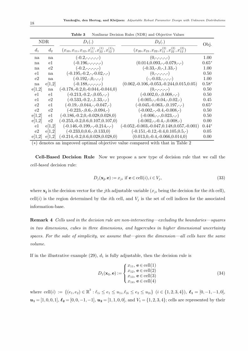
Cell-Based Decision Rule Now we propose a new type of decision rule that we call the
cell-based decision rule:
Dj(xj,e) := xji if e∈ cell(i), i∈ Vj, (33)
where xj is the decision vector for the jth adjustable variable (xji being the decision for the ith cell),
cell(i) is the region determined by the ith cell, and Vj is the set of cell indices for the associated
information-base.
Remark 4 Cells used in the decision rule are non-intersecting—excluding the boundaries—squares
in two dimensions, cubes in three dimensions, and hypercubes in higher dimensional uncertainty
spaces. For the sake of simplicity, we assume that—given the dimension—all cells have the same
volume.
If in the illustrative example (29), d1 is fully adjustable, then the decision rule is
D1(x1,e) :=
x11, e∈ cell(1)x12, e∈ cell(2)x13, e∈ cell(3)x14, e∈ cell(4)
(34)
where cell(i) := (e1, e2) ∈ R2: `1i ≤ e1 ≤ u1i, `2i ≤ e2 ≤ u2i (i ∈ 1,2,3,4), `1 = [0,−1,−1,0],
u1 = [1,0,0,1], `2 = [0,0,−1,−1], u2 = [1,1,0,0], and V1 = 1,2,3,4; cells are represented by their
Yanıkoglu, den Hertog, and Kleijnen: Adjustable Robust Parameter Design with Unknown Distributions19
center points in (30). To show the difference between full and partial information, we assume that
d1 is adjustable on e1 but not on e2. The associated decision then becomes
D1(x1, e1) :=
x11, e1 ∈ cell(1)x12, e1 ∈ cell(2)
(35)
where cell(1) := e1 ∈ R : 0 ≤ e1 ≤ 1 and cell(2) := e1 ∈ R : −1 ≤ e1 ≤ 0, and V1 = 1,2). It is
easy to see that (35) implies that when e2 is extracted from the information-base, the new cells are
projections from the cells in the two-dimensional space in (34) onto the one-dimensional space on
e1 in (35). The disadvantage of the cell-based decision rule is that this rule often has more variables
compared with the linear and nonlinear decision rules, especially when the number of cells is high.
Nevertheless the numerical results for the example show that the new decision rule is better than
the linear, and is ‘almost’ as good as the nonlinear decision rule—even when the total number of
cells is only four; see Table 4.
Table 4 Cell-Based Decision Rules (CDR) and Objective Values
CDR D1(.) D2(.) Obj.d1 d2 (x11, x12, x13, x14) (x21, x22, x23, x24)
na na (-0.2,−,−,−) (0,−,−,−) 1.00na e1 (-0.19,−,−,−) (-0.06,0.04,−,−) 0.66na e2 (-0.2,−,−,−) (0,0,−,−) 1.00e1 na (-0.3,-0.1,−,−) (0,−,−,−) 0.50e2 na (-0.2,-0.2,−,−) (0,−,−,−) 1.00na e[1,2] (-0.19,−,−,−) (-0.09,0.03,0.07,-0.05) 0.62
e[1,2] na (-0.3,-0.1,-0.1,-0.3) (0,−,−,−) 0.50e1 e1 (-0.3,-0.1,−,−) (0,0,−,−) 0.50e1 e2 (-0.3,-0.1,−,−) (-0.02,0.02,−,−) 0.45e2 e1 (-0.18,-0.2,−,−) (-0.06,0.04,−,−) 0.65e2 e2 (0.1,-0.5,−,−) (-0.2,0.2,−,−) 0.50
e[1,2] e1 (-0.3,-0.1,-0.1,-0.3) (0,0,−,−) 0.50e[1,2] e2 (0,0.2,-0.4,-0.6) (-0.2,0.2,−,−) 0.00
e1 e[1,2] (-0.3,-0.1,−,−) (-0.02,-0.02,0.02,0.02) 0.45e2 e[1,2] (0.1,-0.5,−,−) (-0.26,-0.14,0.26,0.14) 0.05
e[1,2] e[1,2] (0,0.2,-0.4,-0.6) (-0.2,-0.2,0.2,0.2) 0.00
To the best of our knowledge, decision rules in the RO literature cannot handle adjustable integer
variables, since the adjustable decision is a function of the uncertain parameter e, and the function
does not necessarily take integer values for all e; see (31) and (32). However, our cell-based decision
rule can handle such variables. As we can see from (33), the adjustable decision xji can take integer
values since the cell-based decision rule relates e and xij through an ‘if’ statement. Therefore, if
we make xij an integer variable, then the cell-based decision rule gives integer decisions. Using the
illustrative example, we show the validity of our approach for such a problem. We modify the old
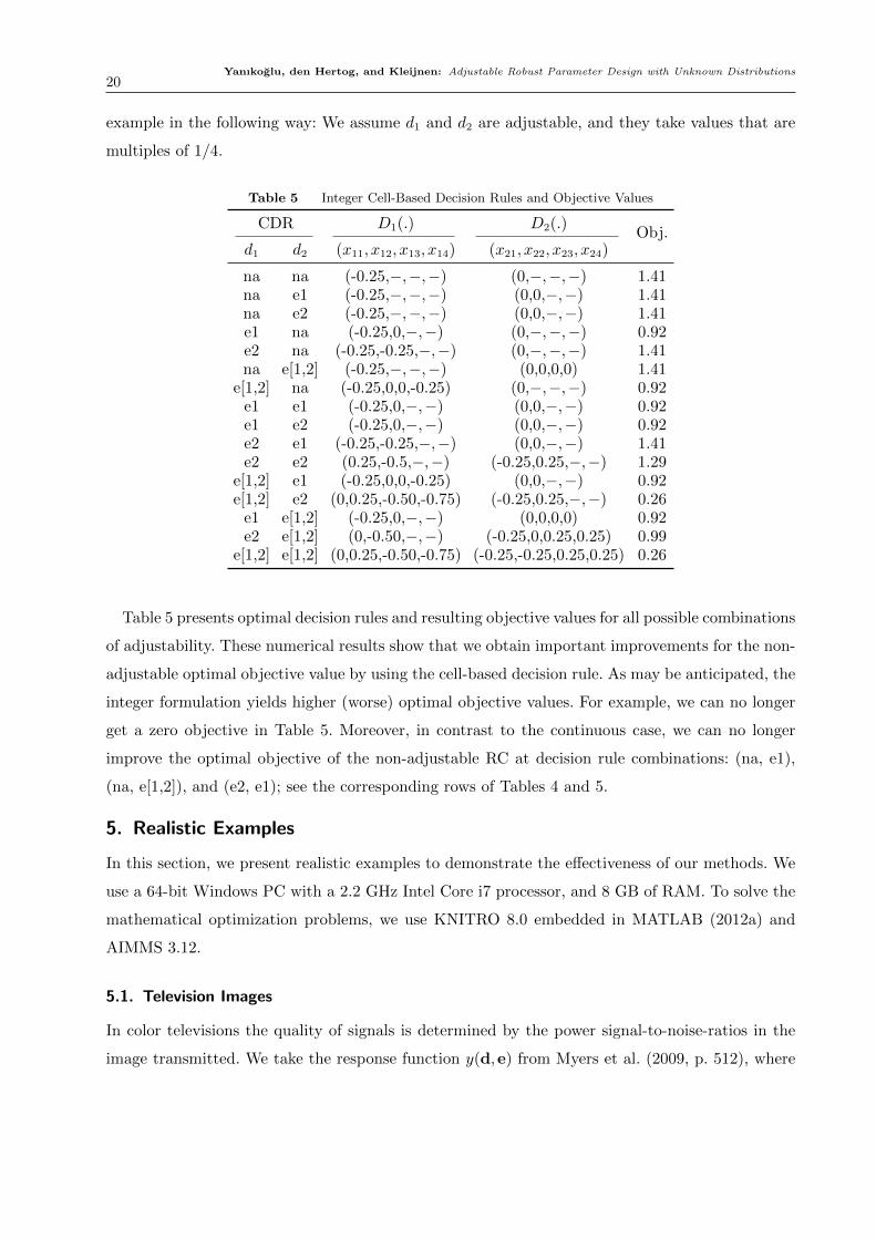
Yanıkoglu, den Hertog, and Kleijnen: Adjustable Robust Parameter Design with Unknown Distributions20
example in the following way: We assume d1 and d2 are adjustable, and they take values that are
multiples of 1/4.
Table 5 Integer Cell-Based Decision Rules and Objective Values
CDR D1(.) D2(.) Obj.d1 d2 (x11, x12, x13, x14) (x21, x22, x23, x24)
na na (-0.25,−,−,−) (0,−,−,−) 1.41na e1 (-0.25,−,−,−) (0,0,−,−) 1.41na e2 (-0.25,−,−,−) (0,0,−,−) 1.41e1 na (-0.25,0,−,−) (0,−,−,−) 0.92e2 na (-0.25,-0.25,−,−) (0,−,−,−) 1.41na e[1,2] (-0.25,−,−,−) (0,0,0,0) 1.41
e[1,2] na (-0.25,0,0,-0.25) (0,−,−,−) 0.92e1 e1 (-0.25,0,−,−) (0,0,−,−) 0.92e1 e2 (-0.25,0,−,−) (0,0,−,−) 0.92e2 e1 (-0.25,-0.25,−,−) (0,0,−,−) 1.41e2 e2 (0.25,-0.5,−,−) (-0.25,0.25,−,−) 1.29
e[1,2] e1 (-0.25,0,0,-0.25) (0,0,−,−) 0.92e[1,2] e2 (0,0.25,-0.50,-0.75) (-0.25,0.25,−,−) 0.26
e1 e[1,2] (-0.25,0,−,−) (0,0,0,0) 0.92e2 e[1,2] (0,-0.50,−,−) (-0.25,0,0.25,0.25) 0.99
e[1,2] e[1,2] (0,0.25,-0.50,-0.75) (-0.25,-0.25,0.25,0.25) 0.26
Table 5 presents optimal decision rules and resulting objective values for all possible combinations
of adjustability. These numerical results show that we obtain important improvements for the non-
adjustable optimal objective value by using the cell-based decision rule. As may be anticipated, the
integer formulation yields higher (worse) optimal objective values. For example, we can no longer
get a zero objective in Table 5. Moreover, in contrast to the continuous case, we can no longer
improve the optimal objective of the non-adjustable RC at decision rule combinations: (na, e1),
(na, e[1,2]), and (e2, e1); see the corresponding rows of Tables 4 and 5.
5. Realistic Examples
In this section, we present realistic examples to demonstrate the effectiveness of our methods. We
use a 64-bit Windows PC with a 2.2 GHz Intel Core i7 processor, and 8 GB of RAM. To solve the
mathematical optimization problems, we use KNITRO 8.0 embedded in MATLAB (2012a) and
AIMMS 3.12.
5.1. Television Images
In color televisions the quality of signals is determined by the power signal-to-noise-ratios in the
image transmitted. We take the response function y(d,e) from Myers et al. (2009, p. 512), where
Yanıkoglu, den Hertog, and Kleijnen: Adjustable Robust Parameter Design with Unknown Distributions21
the response y measures the quality of transmitted signals in decibels. The controllable factors are
the number of tabs in a filter d1, and the sampling frequency d2; the environmental factors are
the number of bits in an image e1, and the voltage applied e2. The least-square estimate of the
metamodel is
y(d,e) = 33.389− 4.175d1 + 3.748d2 + 3.348d1d2− 2.328d21− 1.867d22
− 4.076e1 + 2.985e2− 2.324d1e1 + 1.932d1e2 + 3.268d2e1− 2.073d2e2
where all factors are coded; for details on the DoE we refer to Myers et al. (2009, pp. 511–515).
We find the optimal design settings of d1 and d2 using the optimization problem (9):
maxd
Ee[y(d,e)]
s.t. Vare[y(d,e)]≤ T.(36)
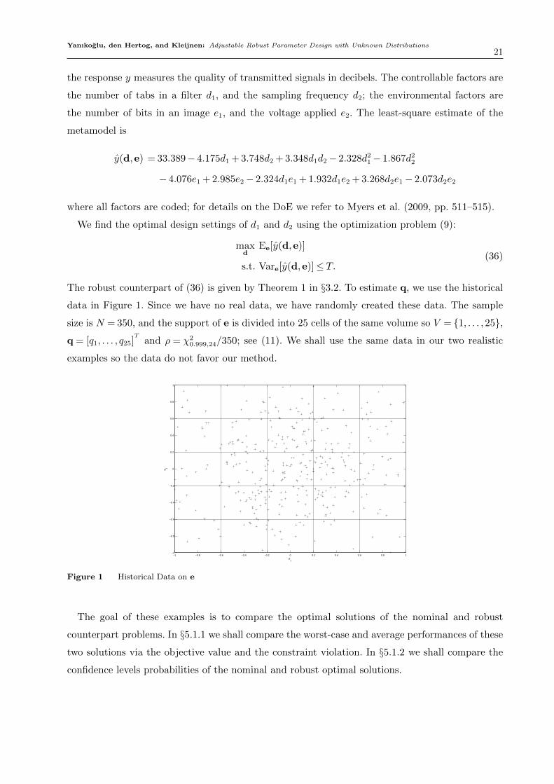
The robust counterpart of (36) is given by Theorem 1 in §3.2. To estimate q, we use the historical
data in Figure 1. Since we have no real data, we have randomly created these data. The sample
size is N = 350, and the support of e is divided into 25 cells of the same volume so V = 1, . . . ,25,
q = [q1, . . . , q25]T
and ρ = χ20.999,24/350; see (11). We shall use the same data in our two realistic
examples so the data do not favor our method.
−1 −0.8 −0.6 −0.4 −0.2 0 0.2 0.4 0.6 0.8 1−1
−0.8
−0.6
−0.4
−0.2
0
0.2
0.4
0.6
0.8
1
e1
e 2
Figure 1 Historical Data on e
The goal of these examples is to compare the optimal solutions of the nominal and robust
counterpart problems. In §5.1.1 we shall compare the worst-case and average performances of these
two solutions via the objective value and the constraint violation. In §5.1.2 we shall compare the
confidence levels probabilities of the nominal and robust optimal solutions.
Yanıkoglu, den Hertog, and Kleijnen: Adjustable Robust Parameter Design with Unknown Distributions22
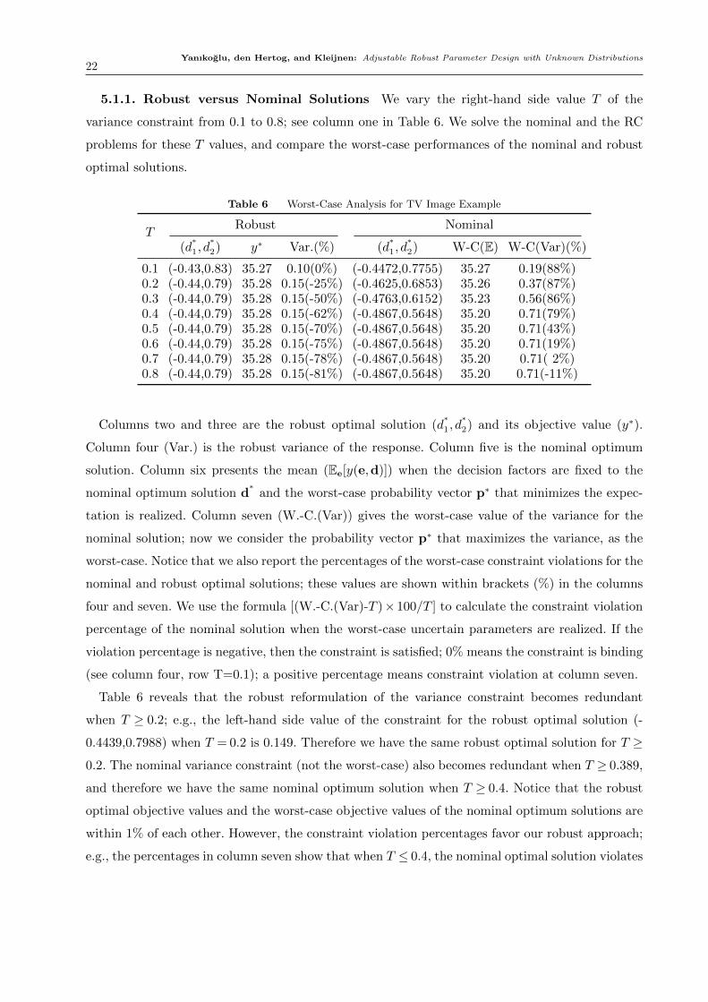
5.1.1. Robust versus Nominal Solutions We vary the right-hand side value T of the
variance constraint from 0.1 to 0.8; see column one in Table 6. We solve the nominal and the RC
problems for these T values, and compare the worst-case performances of the nominal and robust
optimal solutions.
Table 6 Worst-Case Analysis for TV Image Example
TRobust Nominal
(d∗1, d
∗2) y∗ Var.(%) (d
∗1, d
∗2) W-C(E) W-C(Var)(%)
0.1 (-0.43,0.83) 35.27 0.10(0%) (-0.4472,0.7755) 35.27 0.19(88%)0.2 (-0.44,0.79) 35.28 0.15(-25%) (-0.4625,0.6853) 35.26 0.37(87%)0.3 (-0.44,0.79) 35.28 0.15(-50%) (-0.4763,0.6152) 35.23 0.56(86%)0.4 (-0.44,0.79) 35.28 0.15(-62%) (-0.4867,0.5648) 35.20 0.71(79%)0.5 (-0.44,0.79) 35.28 0.15(-70%) (-0.4867,0.5648) 35.20 0.71(43%)0.6 (-0.44,0.79) 35.28 0.15(-75%) (-0.4867,0.5648) 35.20 0.71(19%)0.7 (-0.44,0.79) 35.28 0.15(-78%) (-0.4867,0.5648) 35.20 0.71( 2%)0.8 (-0.44,0.79) 35.28 0.15(-81%) (-0.4867,0.5648) 35.20 0.71(-11%)
Columns two and three are the robust optimal solution (d∗1, d
∗2) and its objective value (y∗).
Column four (Var.) is the robust variance of the response. Column five is the nominal optimum
solution. Column six presents the mean (Ee[y(e,d)]) when the decision factors are fixed to the
nominal optimum solution d∗
and the worst-case probability vector p∗ that minimizes the expec-
tation is realized. Column seven (W.-C.(Var)) gives the worst-case value of the variance for the
nominal solution; now we consider the probability vector p∗ that maximizes the variance, as the
worst-case. Notice that we also report the percentages of the worst-case constraint violations for the
nominal and robust optimal solutions; these values are shown within brackets (%) in the columns
four and seven. We use the formula [(W.-C.(Var)-T )× 100/T ] to calculate the constraint violation
percentage of the nominal solution when the worst-case uncertain parameters are realized. If the
violation percentage is negative, then the constraint is satisfied; 0% means the constraint is binding
(see column four, row T=0.1); a positive percentage means constraint violation at column seven.
Table 6 reveals that the robust reformulation of the variance constraint becomes redundant
when T ≥ 0.2; e.g., the left-hand side value of the constraint for the robust optimal solution (-
0.4439,0.7988) when T = 0.2 is 0.149. Therefore we have the same robust optimal solution for T ≥
0.2. The nominal variance constraint (not the worst-case) also becomes redundant when T ≥ 0.389,
and therefore we have the same nominal optimum solution when T ≥ 0.4. Notice that the robust
optimal objective values and the worst-case objective values of the nominal optimum solutions are
within 1% of each other. However, the constraint violation percentages favor our robust approach;
e.g., the percentages in column seven show that when T ≤ 0.4, the nominal optimal solution violates
Yanıkoglu, den Hertog, and Kleijnen: Adjustable Robust Parameter Design with Unknown Distributions23
the constraint on average 85% in the worst-case. When T ≥ 0.715 the nominal optimum solution
no longer violates the constraint in the worst-case, but it is closer to be binding than the robust
solution. All together, using our robust optimization method for this example, we gain immunity
to the worst-case uncertainty without being penalized by the objective.
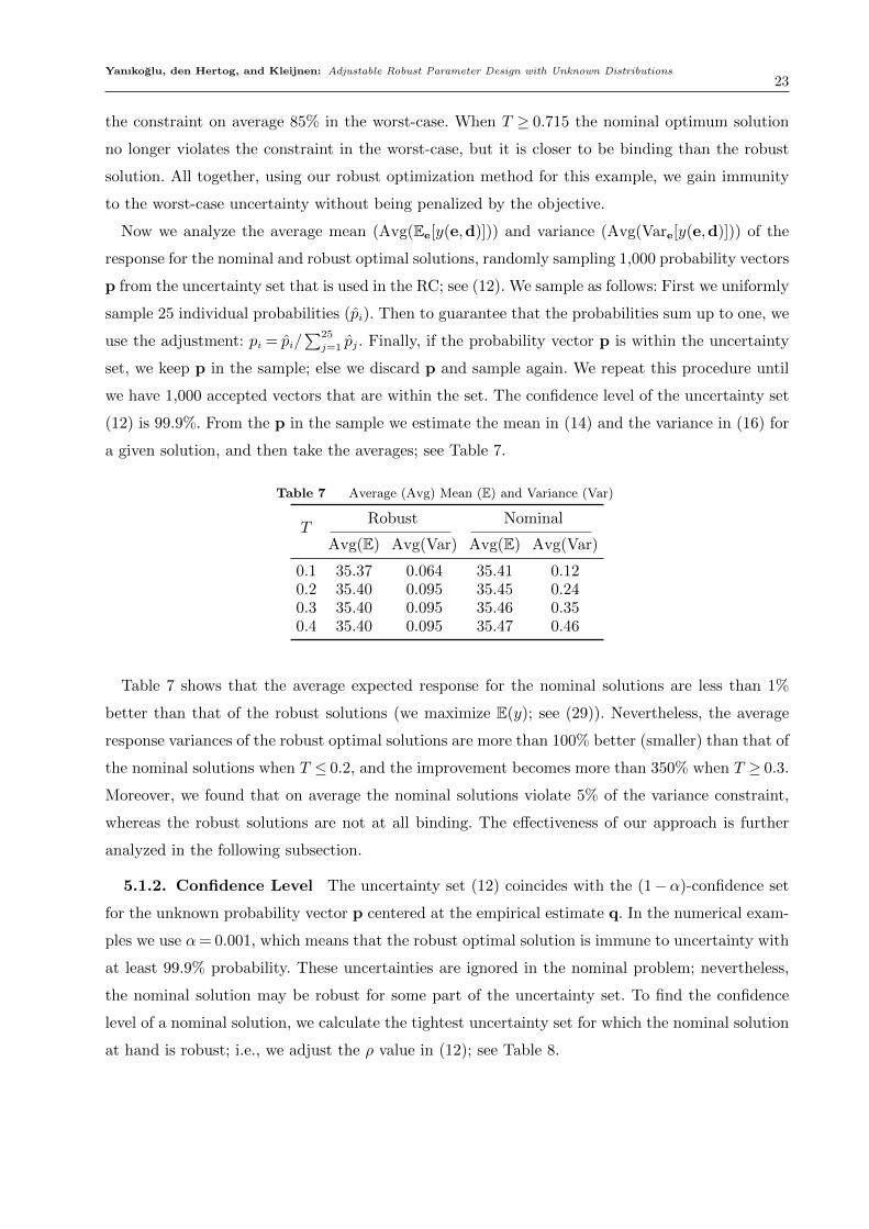
Now we analyze the average mean (Avg(Ee[y(e,d)])) and variance (Avg(Vare[y(e,d)])) of the
response for the nominal and robust optimal solutions, randomly sampling 1,000 probability vectors
p from the uncertainty set that is used in the RC; see (12). We sample as follows: First we uniformly
sample 25 individual probabilities (pi). Then to guarantee that the probabilities sum up to one, we
use the adjustment: pi = pi/∑25
j=1 pj. Finally, if the probability vector p is within the uncertainty
set, we keep p in the sample; else we discard p and sample again. We repeat this procedure until
we have 1,000 accepted vectors that are within the set. The confidence level of the uncertainty set
(12) is 99.9%. From the p in the sample we estimate the mean in (14) and the variance in (16) for
a given solution, and then take the averages; see Table 7.
Table 7 Average (Avg) Mean (E) and Variance (Var)
TRobust Nominal
Avg(E) Avg(Var) Avg(E) Avg(Var)
0.1 35.37 0.064 35.41 0.120.2 35.40 0.095 35.45 0.240.3 35.40 0.095 35.46 0.350.4 35.40 0.095 35.47 0.46
Table 7 shows that the average expected response for the nominal solutions are less than 1%
better than that of the robust solutions (we maximize E(y); see (29)). Nevertheless, the average
response variances of the robust optimal solutions are more than 100% better (smaller) than that of
the nominal solutions when T ≤ 0.2, and the improvement becomes more than 350% when T ≥ 0.3.
Moreover, we found that on average the nominal solutions violate 5% of the variance constraint,
whereas the robust solutions are not at all binding. The effectiveness of our approach is further
analyzed in the following subsection.
5.1.2. Confidence Level The uncertainty set (12) coincides with the (1−α)-confidence set
for the unknown probability vector p centered at the empirical estimate q. In the numerical exam-
ples we use α= 0.001, which means that the robust optimal solution is immune to uncertainty with
at least 99.9% probability. These uncertainties are ignored in the nominal problem; nevertheless,
the nominal solution may be robust for some part of the uncertainty set. To find the confidence
level of a nominal solution, we calculate the tightest uncertainty set for which the nominal solution
at hand is robust; i.e., we adjust the ρ value in (12); see Table 8.
Yanıkoglu, den Hertog, and Kleijnen: Adjustable Robust Parameter Design with Unknown Distributions24
Table 8 Confidence Levels (1-α) of Nominal Solutions
T ≤ 0.4 0.5 0.6 0.7 ≥ 0.8
(1−α) 0% 2% 70% 98% 99.9%
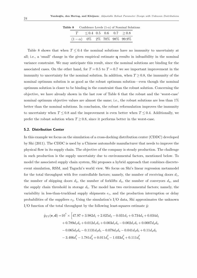
Table 8 shows that when T ≤ 0.4 the nominal solutions have no immunity to uncertainty at
all; i.e., a ‘small’ change in the given empirical estimate q results in infeasibility in the nominal
variance constraint. We may anticipate this result, since the nominal solutions are binding for the
associated cases. On the other hand, for T = 0.5 to T = 0.7 we see important improvement in the
immunity to uncertainty for the nominal solution. In addition, when T ≥ 0.8, the immunity of the
nominal optimum solution is as good as the robust optimum solution—even though the nominal
optimum solution is closer to be binding in the constraint than the robust solution. Concerning the
objective, we have already shown in the last row of Table 6 that the robust and the ‘worst-case’
nominal optimum objective values are almost the same; i.e., the robust solutions are less than 1%
better than the nominal solutions. In conclusion, the robust reformulation improves the immunity
to uncertainty when T ≤ 0.8 and the improvement is even better when T ≤ 0.4. Additionally, we
prefer the robust solution when T ≥ 0.8, since it performs better in the worst-case.
5.2. Distribution Center
In this example we focus on the simulation of a cross-docking distribution center (CDDC) developed
by Shi (2011). The CDDC is used by a Chinese automobile manufacturer that needs to improve the
physical flow in its supply chain. The objective of the company is steady production. The challenge
in such production is the supply uncertainty due to environmental factors, mentioned below. To
model the associated supply chain system, Shi proposes a hybrid approach that combines discrete-
event simulation, RSM, and Taguchi’s world view. We focus on Shi’s linear regression metamodel
for the total throughput with five controllable factors; namely, the number of receiving doors d1,
the number of shipping doors d2, the number of forklifts d3, the number of conveyors d4, and
the supply chain threshold in storage d5. The model has two environmental factors; namely, the
variability in less-than-truckload supply shipments e1, and the production interruption or delay
probabilities of the suppliers e2. Using the simulation’s I/O data, Shi approximates the unknown
I/O function of the total throughput by the following least-squares estimate y:
yTT(e,d) =104
×[47.97 + 3.982d1 + 2.025d2− 0.031d3 + 0.734d4 + 0.034d5
+ 0.789d1d2 + 0.012d1d3 + 0.003d1d4− 0.002d1d5 + 0.0007d2d3
− 0.065d2d4− 0.1131d2d5− 0.078d3d4− 0.041d3d5 + 0.11d4d5
− 3.406d2
1− 1.781d2
2 + 0.011d2
3− 1.033d2
4 + 0.111d2
5
Yanıkoglu, den Hertog, and Kleijnen: Adjustable Robust Parameter Design with Unknown Distributions25
+ (16.66 + 1.511d1 + 2.374d2− 0.059d3 + 0.824d4− 0.093d5)e1
− (0.005 + 0.27d1 + 0.661d2− 0.086d3 + 0.335d4− 0.005d5)e2
],
where all factors are coded such that −1 ≤ d ≤ 1, and −1 ≤ e ≤ 1. More precisely, the coded
controllable factors are between -1 and 1 because of the physical restrictions of the production
facility. Shi’s ANOVA shows that the metamodel yTT have non-significant lack-of-fit; and for the
estimated parameters the level-of-significance is 0.05. Using Shi’s response model, we focus on the
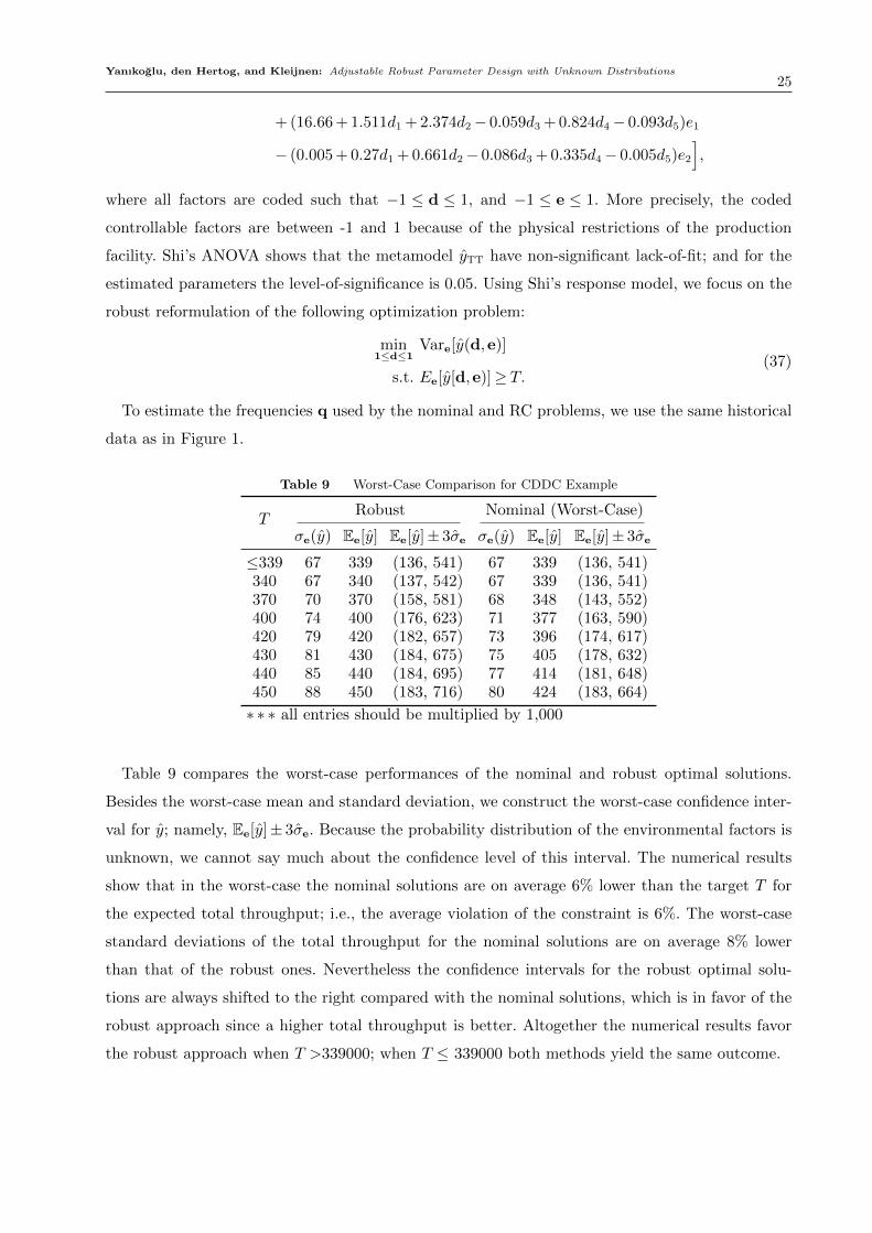
robust reformulation of the following optimization problem:
min1≤d≤1
Vare[y(d,e)]
s.t. Ee[y[d,e)]≥ T.(37)
To estimate the frequencies q used by the nominal and RC problems, we use the same historical
data as in Figure 1.
Table 9 Worst-Case Comparison for CDDC Example
TRobust Nominal (Worst-Case)
σe(y) Ee[y] Ee[y]± 3σe σe(y) Ee[y] Ee[y]± 3σe
≤339 67 339 (136, 541) 67 339 (136, 541)340 67 340 (137, 542) 67 339 (136, 541)370 70 370 (158, 581) 68 348 (143, 552)400 74 400 (176, 623) 71 377 (163, 590)420 79 420 (182, 657) 73 396 (174, 617)430 81 430 (184, 675) 75 405 (178, 632)440 85 440 (184, 695) 77 414 (181, 648)450 88 450 (183, 716) 80 424 (183, 664)
∗ ∗ ∗ all entries should be multiplied by 1,000
Table 9 compares the worst-case performances of the nominal and robust optimal solutions.
Besides the worst-case mean and standard deviation, we construct the worst-case confidence inter-
val for y; namely, Ee[y]± 3σe. Because the probability distribution of the environmental factors is
unknown, we cannot say much about the confidence level of this interval. The numerical results
show that in the worst-case the nominal solutions are on average 6% lower than the target T for
the expected total throughput; i.e., the average violation of the constraint is 6%. The worst-case
standard deviations of the total throughput for the nominal solutions are on average 8% lower
than that of the robust ones. Nevertheless the confidence intervals for the robust optimal solu-
tions are always shifted to the right compared with the nominal solutions, which is in favor of the
robust approach since a higher total throughput is better. Altogether the numerical results favor
the robust approach when T >339000; when T ≤ 339000 both methods yield the same outcome.
Yanıkoglu, den Hertog, and Kleijnen: Adjustable Robust Parameter Design with Unknown Distributions26
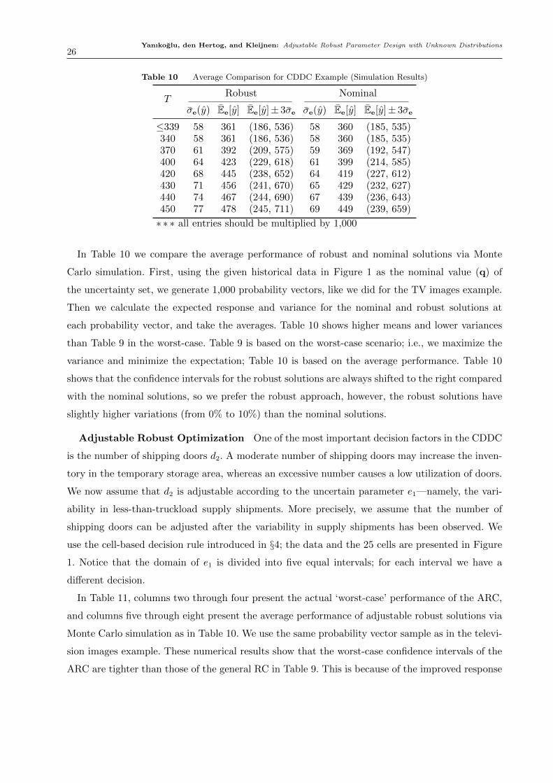
Table 10 Average Comparison for CDDC Example (Simulation Results)
TRobust Nominal
σe(y) Ee[y] Ee[y]± 3σe σe(y) Ee[y] Ee[y]± 3σe
≤339 58 361 (186, 536) 58 360 (185, 535)340 58 361 (186, 536) 58 360 (185, 535)370 61 392 (209, 575) 59 369 (192, 547)400 64 423 (229, 618) 61 399 (214, 585)420 68 445 (238, 652) 64 419 (227, 612)430 71 456 (241, 670) 65 429 (232, 627)440 74 467 (244, 690) 67 439 (236, 643)450 77 478 (245, 711) 69 449 (239, 659)
∗ ∗ ∗ all entries should be multiplied by 1,000
In Table 10 we compare the average performance of robust and nominal solutions via Monte
Carlo simulation. First, using the given historical data in Figure 1 as the nominal value (q) of
the uncertainty set, we generate 1,000 probability vectors, like we did for the TV images example.
Then we calculate the expected response and variance for the nominal and robust solutions at
each probability vector, and take the averages. Table 10 shows higher means and lower variances
than Table 9 in the worst-case. Table 9 is based on the worst-case scenario; i.e., we maximize the
variance and minimize the expectation; Table 10 is based on the average performance. Table 10
shows that the confidence intervals for the robust solutions are always shifted to the right compared
with the nominal solutions, so we prefer the robust approach, however, the robust solutions have
slightly higher variations (from 0% to 10%) than the nominal solutions.
Adjustable Robust Optimization One of the most important decision factors in the CDDC
is the number of shipping doors d2. A moderate number of shipping doors may increase the inven-
tory in the temporary storage area, whereas an excessive number causes a low utilization of doors.
We now assume that d2 is adjustable according to the uncertain parameter e1—namely, the vari-
ability in less-than-truckload supply shipments. More precisely, we assume that the number of
shipping doors can be adjusted after the variability in supply shipments has been observed. We
use the cell-based decision rule introduced in §4; the data and the 25 cells are presented in Figure
1. Notice that the domain of e1 is divided into five equal intervals; for each interval we have a
different decision.
In Table 11, columns two through four present the actual ‘worst-case’ performance of the ARC,
and columns five through eight present the average performance of adjustable robust solutions via
Monte Carlo simulation as in Table 10. We use the same probability vector sample as in the televi-
sion images example. These numerical results show that the worst-case confidence intervals of the
ARC are tighter than those of the general RC in Table 9. This is because of the improved response
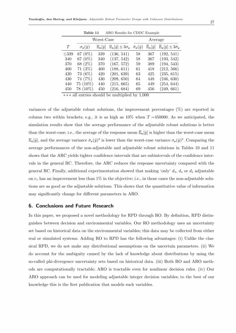
Yanıkoglu, den Hertog, and Kleijnen: Adjustable Robust Parameter Design with Unknown Distributions27
Table 11 ARO Results for CDDC Example
Worst-Case Average
T σe(y) Ee[y] Ee[y]± 3σe σe(y) Ee[y] Ee[y]± 3σe
≤339 67 (0%) 339 (136, 541) 58 367 (192, 541)340 67 (0%) 340 (137, 542) 58 367 (193, 542)370 68 (2%) 370 (167, 572) 59 389 (194, 543)400 71 (3%) 400 (188, 611) 61 418 (212, 566)420 73 (6%) 420 (201, 639) 63 425 (235, 615)430 74 (7%) 430 (209, 650) 64 448 (246, 630)440 75 (10%) 440 (215, 665) 65 449 (254, 644)450 78 (10%) 450 (216, 684) 69 456 (249, 661)
∗ ∗ ∗ all entries should be multiplied by 1,000
variances of the adjustable robust solutions, the improvement percentages (%) are reported in
column two within brackets; e.g., it is as high as 10% when T =450000. As we anticipated, the
simulation results show that the average performance of the adjustable robust solutions is better
than the worst-case; i.e., the average of the response mean Ee[y] is higher than the worst-case mean
Ee[y], and the average variance σe(y)2 is lower than the worst-case variance σe(y)2. Comparing the
average performances of the non-adjustable and adjustable robust solutions in Tables 10 and 11
shows that the ARC yields tighter confidence intervals that are subintervals of the confidence inter-
vals in the general RC. Therefore, the ARC reduces the response uncertainty compared with the
general RC. Finally, additional experimentation showed that making ‘only’ d3, d4 or d5 adjustable
on e1 has an improvement less than 1% in the objective; i.e., in those cases the non-adjustable solu-
tions are as good as the adjustable solutions. This shows that the quantitative value of information
may significantly change for different parameters in ARO.
6. Conclusions and Future Research
In this paper, we proposed a novel methodology for RPD through RO. By definition, RPD distin-
guishes between decision and environmental variables. Our RO methodology uses an uncertainty
set based on historical data on the environmental variables; this data may be collected from either
real or simulated systems. Adding RO to RPD has the following advantages: (i) Unlike the clas-
sical RPD, we do not make any distributional assumptions on the uncertain parameters. (ii) We
do account for the ambiguity caused by the lack of knowledge about distributions by using the
so-called phi-divergence uncertainty sets based on historical data. (iii) Both RO and ARO meth-
ods are computationally tractable; ARO is tractable even for nonlinear decision rules. (iv) Our
ARO approach can be used for modeling adjustable integer decision variables; to the best of our
knowledge this is the first publication that models such variables.

Yanıkoglu, den Hertog, and Kleijnen: Adjustable Robust Parameter Design with Unknown Distributions28
In future research, we shall investigate our methodology for other metamodel types, such as
higher-order polynomials, Kriging, and radial basis functions. We shall also apply our cell-based
decision rules to general classes of optimization problems with limited number of ‘integer’ variables.
References
Al-Aomar, R. 2006. Incorporating robustness into genetic algorithm search of stochastic simulation outputs.
Simulation Modelling Practice and Theory 14(3) 201–223.
Angun, E. 2011. A risk-averse approach to simulation optimization with multiple responses. Simulation
Model. Practices and Theory 19(3) 911–923.
Ben-Tal, A., A. Nemirovski. 1998. Robust convex optimization. Math. Oper. Res. 23(4) 769–805.
Ben-Tal, A., A. Nemirovski. 1999. Robust solutions of uncertain linear programs. Oper. Res. Lett. 25(1)
1–13.
Ben-Tal, A., D. den Hertog, J.-P. Vial. 2012. Deriving robust counterparts of nonlinear uncertain inequalities.
CentER Discussion Paper No. 2012-053, Tilburg University, Tilburg, The Netherlands.
Ben-Tal, A., L. El Ghaoui, A. Nemirovski. 2009. Robust Optimization. Princeton Press, Princeton, NJ.
Ben-Tal, A., D. den Hertog, A. De Waegenaere, B. Melenberg, G. Rennen. 2013. Robust solutions of opti-
mization problems affected by uncertain probabilities. Management Sci. 59(2) 341–357.
Bingham, D., V. N. Nair. 2012. Noise variable settings in robust design experiments. Technometrics 54(4)
388–397.
Chan, Y.-J., D. J. Ewins. 2010. Management of the variability of vibration response levels in mistuned bladed
discs using robust design concepts. Mech. Systems and Signal Processing Part 1: Parameter Design
24(8) 2777–2791.
Dasgupta, T., C. F. J. Wu. 2006. Robust Parameter design with feed-back control. Technometrics 48(3)
349–359.
Dellino, G., J. P. C. Kleijnen, C. Meloni. 2012. Robust optimization in simulation: Taguchi and Krige
combined INFORMS J. Comput. 24(3) 471–484.
Delpiano, J., M. Sepulveda. 2006. Combining iterative heuristic optimization and uncertainty analysis meth-
ods for robust parameter design. Engineering Optim. 38(7) 821–831.
El-Ghaoui, L., H. Lebret. 1997. Robust solutions to least-squares problems with uncertain data. SIAM. J.
Matrix Anal. & Appl. 18(4) 1035–1064.
Fu, M. C. 2007. Are we there yet? The marriage between simulation & optimization. OR/MS Today 34(3)
16–17.
Fu, M., B. Nelson. 2003. Simulation optimization. ACM Trans. Model. and Simulation 13(2) 105–107.
Yanıkoglu, den Hertog, and Kleijnen: Adjustable Robust Parameter Design with Unknown Distributions29
Hu, Zhaolin, J. Cao, L. J. Hong. 2012. Robust simulation of global warming policies using the DICE model.
Management Sci. 58(13) 2190–2206.
Iman, R. L., J. C. Helton. 2006. An investigation of uncertainty and sensitivity analysis techniques for
computer models. Risk Anal. 8(1) 71–90.
Joseph, V. R. 2003. Robust parameter design with feed-forward control. Technometrics 45(4) 284–292.
Kleijnen, J. P. C. 2008. Design and Analysis of Simulation Experiments. Springer-Verlag, Heidelberg, Ger-
many.
Miranda, A. K., E. del Castillo. 2011. Robust parameter design optimization of simulation experiments using
stochastic perturbation methods. J. Oper. Res. Soc. 62(1) 198–205.
Myers, R. H., D. C. Montgomery, C. M. Anderson-Cook. 2009. Response Surface Methodology: Process and
Product Optimization Using Designed Experiments, 3rd ed. John Wiley & Sons, Hoboken, NJ.
Nair, V. N., B. Abraham, J. MacKay, G. Box, R. N. Kacker, T. J. Lorenzen, J. M. Lucas. 1992. Taguchi’s
parameter design: a panel discussion. Technometrics 34(2) 127–161.
Pardo, L. 2006. Statistical Inference Based on Divergence Measures. Chapman & Hall/CRC, Boca Raton,
FL.
Rockafellar, R. T. 1970. Convex Analysis. Princeton University Press, Princeton, NJ.
Sanchez, S. M. 2000. Robust design: seeking the best of all possible worlds. Proceedings of the 2000 Winter
Simulation Conference (edited by J.A. Joines, R.R. Barton, K Kang, and P.A. Fishwick) 1 69–76.
Shi, W. 2011. Design of pre-enhanced cross-docking distribution center under supply uncertainty: RSM
robust optimization method. Working Paper, Huazhong University of Science & Technology, China.
Spall, J. 2003. Introduction to Stochastic Search and Optimization. Wiley-Interscience, New York, NY.
Taguchi, G. 1986. Introduction to Quality Engineering. Asian Productivity Organization, UNIPUB, White
Plains, NY.
Taguchi, G. 1987. System of Experimental Design: Engineering Methods to Optimize Quality and Minimize
Cost. UNIPUB/Kraus International, White Plains, NY.
Urval, R., S. Lee, S. V. Atre, S.-J. Park, R. M. German. 2010. Optimisation of process conditions in powder
injection moulding of microsystem components using robust design method. Powder Metallurgy Part
2: Secondary Design Parameters 53(1) 71–81.
Vanlı, O. A., E. Del Castillo. 2009. Bayesian approaches for on-line robust parameter design. IIE Transactions
41(4) 359–371.
Wiedemann, M. 2010. Robust Parameter Design for Agent-Based Simulation Models With Application in a
Cultural Geography Model. Master’s Thesis, Naval Postgraduate School, Monterey, CA.
Yanıkoglu, I., D. den Hertog. 2012. Safe approximations of ambiguous chance constraints using historical
data. INFORMS J. Comput. forthcoming.