· this book forms the proceedings of mam10, and contains 34 abstracts, including 7 extended...

Proceedings

Tenth International Conference on Matrix-AnalyticMethods in Stochastic Models

Editors

SOPHIE HAUTPHENNEThe University of Melbourne

Victoria 3010, Australia

MA LGORZATA O’REILLYSchool of Natural Sciences

University of TasmaniaTasmania 7005, Australia

FEDERICO POLONIDepartment of Computer Science

University of Pisa56127 Pisa, Italy

c©2019 Discipline of Mathematics, University of Tasmania. Copyright for the abstracts appearing in theseproceedings is held by the owner/author(s).

ISBN: 978-0-646-99707-0 (Print version, soft cover)ISBN: 978-0-646-99825-1 (Electronic version)

Printed in 2019, Hobart, Australia.

5

Note from the editorsOver the years, matrix-analytic models have proved to be successful in providing performance measures for alarge number of real-world systems. In their corresponding computational methods, known as matrix-analyticmethods, algorithmic issues are investigated in detail and the probabilistic interpretation of the proposed numericalprocedures plays a major role. These methods have been developed initially in the context of queueing models andhave given rise to the theory of quasi-birth-and-death processes and of skip-free Markov chains, both belonging tothe class of structured Markov chains. More recently, matrix-analytic methods have been extended further forstochastic fluid queues, branching processes, and Markov-modulated Brownian motion.

The Tenth International Conference on Matrix-Analytic Methods in Stochastic Models (MAM10) was held at theUniversity of Tasmania in Hobart from the 13th to the 15th of February 2019, continuing the established traditionof previous fruitful MAM conferences in Flint (1995), Winnipeg (1998), Leuven (2000), Adelaide (2002), Pisa(2005), Beijing (2008), New York (2011), Calicut (2014), and Budapest (2016).

The MAM10 conference was sponsored by the Australian Mathematical Sciences Institute (AMSI), the AustralianMathematical Society (AustMS), the Australian Research Council Centre of Excellence for Mathematical andStatistical Frontiers (ACEMS), as well as by Peter Taylor (Australian Laureate Fellow, at the University ofMelbourne, Director of ACEMS) and Andrew Bassom (Head of Discipline – Mathematics, University of Tasmania).

MAM conferences aim to bring together researchers working on the theoretical, algorithmic and methodologicalaspects of these methods and the applications of such mathematical research across a broad spectrum of fields,which includes computer science and engineering, telephony and communication networks, electrical and industrialengineering, operations research, management science, financial and risk analysis, bio-statistics, and evolution.

This book forms the Proceedings of MAM10, and contains 34 abstracts, including 7 extended abstracts. Eachextended abstract was reviewed anonymously by two members of the program committee. Keynote talks weregiven by Azam Asanjarani, Søren Asmussen, Jevgenijs Ivanovs, Giang Nguyen, Zbigniew Palmowski, and PhilPollett.

We thank our steering committee and program committee members, and all other people who helped in theorganization of the conference. We thank the University of Tasmania for hosting the conference, and our sponsorsfor their financial support. We thank all the authors who contributed to the abstracts, the reviewers, and all theparticipants. We thank Odyseusz Zawalski for the design of the poster, the MAM logo, and the cover of this book.We thank Kelly Carpenter for the administrative support.

Sophie Hautphenne, Ma lgorzata O’Reilly, and Federico Poloni

6

Organising Committee:

Ma lgorzata O’Reilly, Conference Chair, University of Tasmania, AustraliaSophie Hautphenne, Program Co-Chair, The University of Melbourne, AustraliaFederico Poloni, Program Co-Chair, University of Pisa, ItalyMark Fackrell, The University of Melbourne, AustraliaBarbara Holland, University of Tasmania, AustraliaMichael Brideson, University of Tasmania, Australia

Steering Committee:

Attahiru S. Alfa, University of Manitoba, Canada, and University of Pretoria, South AfricaGuy Latouche, Universite Libre de Bruxelles, BelgiumMiklos Telek, Technical University of Budapest, HungaryPeter Taylor, The University of Melbourne, AustraliaQi-Ming He, University of Waterloo, CanadaV. Ramaswami, Statmetrics, LLC, United States

Program Committee:

Søren Asmussen, Aarhus University, DenmarkNigel Bean, The University of Adelaide, AustraliaPeter Braunsteins, The University of Melbourne, AustraliaPeter Buchholz, Technische Universitat Dortmund, GermanyGiuliano Casale, Imperial College London, UKSrinivas Chakravarthy, Kettering University, United StatesTugrul Dayar, Bilkent University, TurkeyMark Fackrell, The University of Melbourne, AustraliaQi-Ming He, University of Waterloo, CanadaAndras Horvath, Universita di Torino, ItalyGabor Horvath, Budapest University of Technology and Economics, HungaryUdo Krieger, IEEE, GermanyBarbara Margolius, Cleveland State University, United StatesStefano Massei, Ecole Polytechnique Federale de Lausanne, SwitzerlandBeatrice Meini, University of Pisa, ItalyMasakiyo Miyazawa, Tokyo University of Science, JapanYoni Nazarathy, The University of Queensland, AustraliaGiang Nguyen, The University of Adelaide, AustraliaV. Ramaswami, Statmetrics, LLC, United StatesRotislav Razumchik, Russian Academy of Sciences, RussiaAlexander Rumyantsev, Russian Academy of Sciences, RussiaEvgenia Smirni, College William & Mary, United StatesAviva Samuelson, University of Tasmania, AustraliaMark Squillante, IBM, United StatesTetsuya Takine, Osaka University, JapanPeter Taylor, The University of Melbourne, AustraliaMiklos Telek, Technical University of Budapest, HungaryErik van Doorn, University of Twente, NetherlandsBenny van Houdt, University of Antwerp, BelgiumEleni Vatamidou, University of Lausanne, SwitzerlandYiqiang Zhao, Carleton University, Canada

7

Table of Contents

Soohan Ahn and Beatrice Meini Matrix equations in Markov modulated Brownian motion: theoreticalproperties and numerical solution . . . . . . . . . . . . . . . . . . . . . . . . . . . . . . . . . . . . . . 9

Aregawi Kiros Abera, Ma lgorzata O’Reilly, Barbara Holland, Mark Fackrell and Mojtaba Heydar Decisionsupport model for patient admission scheduling problem with random arrivals and departures . . . . . 10

Azam Asanjarani Bursty Markovian Arrival Processes . . . . . . . . . . . . . . . . . . . . . . . . . . . . . . 15

Søren Asmussen On some fixed-point problems connecting branching and queueing . . . . . . . . . . . . . . 16

Nigel Bean, Giang Nguyen, Bo Friis Nielsen and Oscar Peralta A fluid flow model with RAP components . 17

Nigel Bean, Giang T. Nguyen and Federico Poloni A new algorithm for time-dependent first-return probabilitiesof a fluid queue . . . . . . . . . . . . . . . . . . . . . . . . . . . . . . . . . . . . . . . . . . . . . . . . 18

Dario Bini, Stefano Massei, Beatrice Meini and Leonardo Robol Matrix analytic methods for reflected randomwalks with stochastic restarts . . . . . . . . . . . . . . . . . . . . . . . . . . . . . . . . . . . . . . . . 23

Peter Braunsteins and Sophie Hautphenne Extinction in lower Hessenberg branching processes with countablymany types . . . . . . . . . . . . . . . . . . . . . . . . . . . . . . . . . . . . . . . . . . . . . . . . . . 24

Peter Braunsteins and Sophie Hautphenne The probabilities of extinction in a branching random walk on a strip 25

Pavithra Celeste R. and Deepak T.G. On Fisher Information of Some Functions of Phase Type Variates . . 26

Jiahao Diao, Tristan Stark, David Liberles, Ma lgorzata O’Reilly and Barbara Holland Model for the evolutionof the family of gene duplicates . . . . . . . . . . . . . . . . . . . . . . . . . . . . . . . . . . . . . . . 29

Qi-Ming He, Mark Fackrell and Peter Taylor Characterization of the Boundary of the Set of Matrix-ExponentialDistributions with Only Real Poles . . . . . . . . . . . . . . . . . . . . . . . . . . . . . . . . . . . . . 30

Mojtaba Heydar and Ma lgorzata O’Reilly Markovian decision-support model for patient-to-ward assignmentproblem in a random environment . . . . . . . . . . . . . . . . . . . . . . . . . . . . . . . . . . . . . 31

Gabor Horvath, Illes Horvath and Miklos Telek High order low variance matrix-exponential distributions . . 33

Gabor Horvath, Illes Horvath, Salah Almousa and Miklos Telek Numerical Inverse Laplace Transformationby concentrated ME distributions . . . . . . . . . . . . . . . . . . . . . . . . . . . . . . . . . . . . . . 37

Jevgenijs Ivanovs One-sided Markov additive processes: the three fundamental matrices and the scale function 41

Sarah James, Nigel Bean and Jonathan Tuke Modelling intensive care units using quasi-birth-death processes 42

Kayla Javier and Brian Fralix An exact analysis of a class of Markovian Bitcoin models . . . . . . . . . . . 43

Guy Latouche Nearly-completely decomposable Markov modulated fluid queues . . . . . . . . . . . . . . . . . 44

Barbara Margolius Eulerian Numbers and an Explicit Formula for a Random Walk Generating Function . . 45

Barbara Margolius and Ma lgorzata O’Reilly Asymptotic periodic analysis of cyclic stochastic fluid flows withtime-varying transition rates . . . . . . . . . . . . . . . . . . . . . . . . . . . . . . . . . . . . . . . . . 48

Stefano Massei and Sophie Hautphenne A new numerical method for computing the quasi-stationary distribu-tion of subcritical Galton-Watson branching processes . . . . . . . . . . . . . . . . . . . . . . . . . . . 49

Giang Nguyen and Oscar Peralta-Gutierrez Rate of strong convergence of stochastic fluid processes toMarkov-modulated Brownian motion . . . . . . . . . . . . . . . . . . . . . . . . . . . . . . . . . . . . 50

Zbigniew Palmowski One-sided Markov additive processes: exit problems and related topics . . . . . . . . . 51

Phil Pollett Quasi stationarity . . . . . . . . . . . . . . . . . . . . . . . . . . . . . . . . . . . . . . . . . . . 52

Aviva Samuelson, Ma lgorzata O’Reilly and Nigel Bean Construction of algorithms for discrete-time quasi-birth-and-death processes through physical interpretation . . . . . . . . . . . . . . . . . . . . . . . . . 53

Julia Shore, Barbara Holland, Jeremy Sumner, Kay Nieselt and Peter Wills Substitution matrices recapitulateamino acid specificity of aaRS phylogenies . . . . . . . . . . . . . . . . . . . . . . . . . . . . . . . . . 58

Matthieu Simon SIR epidemics with stochastic infectious periods . . . . . . . . . . . . . . . . . . . . . . . . 59

Tristan Stark, Ma lgorzata O’Reilly, Barbara Holland and David Liberles Models for the evolution of gene-duplicates: Applications of Phase-Type distributions . . . . . . . . . . . . . . . . . . . . . . . . . . . . 60

Tristan Stark, Ma lgorzata O’Reilly and Barbara Holland Models for the evolution of microsatellites . . . . 61

Jeremy Sumner and Michael Baake The Markov embedding problem: a new look from an algebraic perspective 62

Jeremy Sumner and Julia Shore Algebraic constraints on the transition probability matrices produced fromLie-Markov models . . . . . . . . . . . . . . . . . . . . . . . . . . . . . . . . . . . . . . . . . . . . . . 63

Venta Terauds and Jeremy Sumner Maximum likelihood rearrangement distance for circular genomes . . . . 64

Max Wurm, Andrew Baird, Nigel Bean, Sean Connolly, Ariella Helfgott and Giang Nguyen Polyp fiction: Astochastic fluid model for the Adaptive Bleaching Hypothesis . . . . . . . . . . . . . . . . . . . . . . . 65

8

Matrix equations in Markov modulated Brownian motion:theoretical properties and numerical solution

Soohan AhnDepartment of Statistics, The University of Seoul

163 Seoulsiripdaero, Dongdaemun-gu, Seoul02504, South [email protected]

Beatrice MeiniDipartimento di Matematica, Università di Pisa

Largo B. Pontecorvo 5, 56127 Pisa, [email protected]

ABSTRACTA Markov modulated Brownian motion(MMBM) is a sub-stantial generalization of the classical Brownian Motion andis obtained by allowing the Brownian parameters to be mod-ulated by an underlying Markov chain of environments [2].As with Brownian Motion, the stationary analysis of theMMBM becomes easy once the distributions of the first pas-sage time between levels are determined. However, in theMMBM those distributions cannot be obtained explicitly,and we need efficient numerical methods to compute them.In particular, in [2], the computation of the distribution isultimately reduced to solving a quadratic matrix equation(QME). In relation to this, Ahn and Ramaswami [1] derived anonsymmetric algebraic Riccati equation(NARE) and provedthat the distributions can be obtained by using the minimalnonnegative solution of the equation.

The contribution of this talk is twofold. From one handwe provide an algebraic connection between the QME andthe NARE, more specifically we show that the NARE can beobtained by means of a linearization of a quadratic matrixpolynomial associated with the QME. On the other hand,we discuss the doubling algorithms such as the structure-preserving doubling algorithm(SDA, [3]) and alternating-directional doubling algorithm(ADDA, [5]) which are usedfor finding the minimal nonnegative solution of the NARE.These algorithms are quadratically convergent except for thenull-recurrent case of the MMBM. To improve the speedof convergence of the doubling algorithms, we introduce ashifted NARE by applying the shift technique, which wasinvestigated by Guo, Iannazzo, and Meini [4]. We observethat the convergence of the doubling algorithms is acceleratedand also quadratic even in the null-recurrent case whenthey are applied to the shifted NARE, as claimed by Guo,Iannazzo, and Meini. Numerical examples show that thealgorithm applying ADDA to the shifted NARE is superiorto the other doubling algorithms in comparison. This alsoholds when compared to Nguyen and Poloni’s quadraticallyconvergent algorithm [6] that is based on the quadratic matrix

Permission to make digital or hard copies of part or all of this work for personal orclassroom use is granted without fee provided that copies are not made or distributedfor profit or commercial advantage and that copies bear this notice and the full citationon the first page. Copyrights for third-party components of this work must be honored.For all other uses, contact the owner/author(s).

MAM10 2019, Hobart, Australia c© 2019 Copyright held by the owner/author(s).

equation obtained by Asmussen.

Keywords : Markov modulated Brownian motion, first pas-sage time distribution, doubling algorithm, quadratic conver-gence, shifted nonsymmetric algebraic Riccati equation.

References[1] S. Ahn and V. Ramaswami. A quadratically conver-

gent algorithm for first passage time distributions in themarkov modulated brownian motion. Stochastic Models,33(1):59–96, 2017.

[2] S. Asmussen. Stationary distributions for fluid flow mod-els with or without brownian noise. Stochastic Models,11:1–20, 1995.

[3] D. A. Bini, B. Iannazzo, and B. Meini. Numerical solutionof algebraic Riccati equations. Siam, Philadelphia, 2012.

[4] C. H. Guo, B. Iannazzo, and B. Meini. On the doublingalgorithm for a shifted nonsymmetric algebraic riccatiequation. SIAM J. Matrix Anal. Appl., 63:109–129, 2007.

[5] X. X. Guo, W. W. Lin, and S. F. Xu. A structure-preserving doubling algorithm for nonsymmetric algebraicriccati equation. Numer. Math., 103:393–412, 2006.

[6] G. T. Nguyen and F. Poloni. Componentwise accuratebrownian motion computations using cyclic reduction.arXiv:1605.01482[math.PR], 2015.

9

Decision support model for the patient admissionscheduling problem with random arrivals and departures

Aregawi K. Abera ∗

University of TasmaniaTAS 7001, Australiaaregawi.abera@

utas.edu.au

Małgorzata M. O’Reilly ∗†

University of TasmaniaTAS 7001, Australia

[email protected]

Barbara R. HollandUniversity of Tasmania

TAS 7001, Australiabarbara.holland@

utas.edu.au

Mark Fackrell ∗†The University of Melbourne

VIC 3010, [email protected]

Mojtaba Heydar ∗

University of TasmaniaTAS 7001, Australia

[email protected]

ABSTRACTIntroduction. The patient admission scheduling (PAS)problem is a class of scheduling problems that must be han-dled by the managers of the hospital admission systems. Theproblem arises when patients arriving at the hospital needto be allocated to beds in an optimal manner, subject to theavailability of beds and the needs of patients.

The PAS problem in a dynamic context, as analysed inCeschia and Schaerf [2] and Lusby et al. [6], considers ascenario in which random arrivals and unknown departuresof patients are gradually revealed over the planning horizon.The problem was formulated as an integer programmingmodel, and various procedures for computing the optimalsolution were proposed. Ceschia and Schaerf [2] developed ametaheuristic algorithm based on simulated annealing andneighborhood search. Lusby et al. [6] developed an adaptivelarge neighbourhood search procedure to solve the problem.

Although the arrivals and departures of patients are ingeneral random, the models in [2, 6] assumed deterministicinputs such as a fixed length of stay for each patient, and afixed number of arrivals at the start of each day. Here, webuild on the analysis in Lusby et al. [6], and develop a modelfor the PAS problem in a dynamic context, which capturesthe random dynamics of the flow of the patients.

Our aim here is to develop an improved mathematicalmodel to solve the PAS problem in a dynamic environment

∗Australian Research Council Centre of Excellence for Math-ematical and Statistical Frontiers.†We would like to thank the Australian Research Council forfunding this research through Linkage Project LP140100152.



with random arrivals and departures. At the start of eachday we record new information about the registered patients,newly arrived patients and future arrivals (including emer-gency patients and scheduled arrivals), and then determinean optimal assignment of patients to beds. Our goal is toprovide a decision support tool for the patient schedulingprocess to be used by hospital administrators and planners.

Notation. We use similar notation to Demeester et al. [3]and Turhan and Bilgen [8] for the parameters and variablesof our model, with some minor changes.

• Patients are classified into three groups, admitted pa-tients, planned patients, and emergency patients. Ad-mitted patients are patients that are successfully ad-mitted to the hospital, and allocated to a bed. Plannedpatients have not been admitted to the hospital asyet, but have pre-determined admission dates, denotedby dplanp . Emergency patients are patients whose ad-mission date is equal to their registration date, thatis, dplanp = dregp , since their admission cannot be post-poned and is unplanned.

• Patients are denoted by p, with p ∈ P, where P isthe set of all patients. Also let M ⊂ P be the setof all male patients, and F ⊂ P be the set of allfemale patients. Patients have the following properties:admission date and a discharge date, age and gender,required treatment, and room preference.

• Days are denoted by d, with d ∈ D, where D =0, 1, . . . , D is the set of all days in the planning periodof the time horizon. Further, let dp ∈ Dp be the admis-sion day of patient p, where Dp = dplanp , · · · , dmaxp ⊆D is the set of acceptable days for patient p to beadmitted to the hospital.

• The length of stay (LoS) of patient p is denoted byLp. This is a random variable recording the numberof days patient p will stay in the hospital till he/shegets discharged. We assume Lp takes values `p =0, 1, . . . , `maxp , for some positive integer `maxp .

• A hospital consists of different wards. Typically, eachward is specialized in treating one kind of pathology

10

such as cardiovascular diseases, oncology, or derma-tology, which is considered as the major specialism ofthe ward as in Demeester et al. [3]. Wards can alsoperform other treatments as minor specialisms. Wardsare denoted by Wi, i = 1, . . . ,W , where W is the totalnumber of wards in the hospital. Wards can supportone or more specialisms Su, u = 1, . . . , S, where S isthe total number of specialisms. We write

Su ∼ Wi (1)

when specialism Su is available in ward Wi, and

S(p) = Su (2)

when patient p requires specialism Su. Patients ad-mitted to ward Wi may have to be in a particular agerange, between some minimum a(Wi) and maximumA(Wi).

• Rooms are denoted by r, with r ∈ R = 1, . . . , R,where R is the total number of rooms in the hospital.We write

r ∈ Wi (3)

when room r is in ward Wi ⊂ R. A room can bedescribed by its age policy, gender policy and by itsspecial features, such as the presence of oxygen, ni-trogen, telemetry or television. A room may supportone or more different specialisms Su, depending on theroom features. Rooms have a specified gender policy,which is one of the following; male only M , femaleonly F , depends on the gender of the first patient SG(same-gender policy), or all genders are allowed N . Itis preferable to not assign male and female patientsto the same room at the same time. We denote byRM ,RF ,RSG,RN ⊂ R the sets of all rooms withpolicies M,F, SG,N , respectively.

• The capacity of room r is denoted by κr. This is thetotal number of beds in room r.

• Assignment σ is the collection of decisions xp,r,d(σ) andyp,d(σ) defined as,

xp,r,d(σ) =

1 if patient p is assignedto room r on day d

0 otherwise,(4)

yp,d(σ) =

1 if patient p isadmitted on day d

0 otherwise,(5)

and note that yp,d(σ) = 1d = dp(σ), where 1. isan indicator function.

• In order to calculate the violation of gender policy, wedefine the presence of male, female and both patientsin room r on day d as follows,

mr,d(σ) =

1 if there is at least one malepatient in room r on day d,

0 otherwise,(6)

fr,d(σ) =

1 if there is at least one femalepatient in room r on day d,

0 otherwise,(7)

br,d(σ) =

1 if both genders are presentin room r on day d,

0 otherwise.(8)

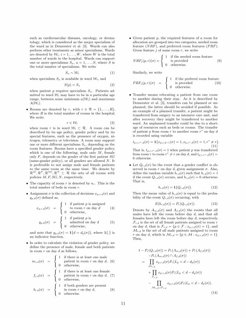
• Given patient p, the required features of a room forallocation are grouped into two categories, needed roomfeature (NRF ), and preferred room features (PRF ).Given feature j of some room r, we write

NRFj(p, r)(σ) =

1 if the needed room featureis provided

0 otherwise.(9)

Similarly, we write

PRFj(p, r)(σ) =

1 if the prefered room featureis provided

0 otherwise.(10)

• Transfer means relocating a patient from one roomto another during their stay. As it is described byDemeester et al. [3], transfers can be planned or un-planned, the latter should be avoided if possible. Asan example of a planned transfer, a patient might betransferred from surgery to an intensive care unit, andafter recovery they might be transferred to anotherward. An unplanned transfer could be due to a short-age of resources such as beds or rooms. The transferof patient p from room r to another room r∗ on day dis recorded using variable

tp,r,r∗,d(σ) = 1xp,r,d−1(σ) = 1, xp,r∗,d(σ) = 1, r∗ 6= r.(11)

That is, tp,r,r∗,d(σ) = 1 when patient p was transferredfrom room r to room r∗ 6= r on day d, and tp,r,r∗,d(σ) =0 otherwise.

• Let Qr,d(σ) be the event that a gender conflict is ob-served in room r on day d, given assignment σ. Also,define the random variable br,d(σ) such that br,d(σ) = 1if the event Qr,d(σ) occurs, and br,d(σ) = 0 otherwise.That is,

br,d(σ) = 1Qr,d(σ). (12)

Then the mean value of br,d(σ) is equal to the proba-bility of the event Qr,d(σ) occurring, with

E(br,d(σ)) = Pr(Qr,d(σ)). (13)

Denote by Am,d(σ) and Af,d(σ) the events that allmales have left the room before day d, and that allfemales have left the room before day d, respectively.Fr,d is the set of all female patients assigned to room ron day d, that is Fr,d = p ∈ F : xp,r,d(σ) = 1, andMr,d is the set of all male patients assigned to roomr on day d, which is Mr,d = p ∈ M : xp,r,d(σ) = 1.Then,

1− Pr(Qr,d(σ)) = Pr(Am,d(σ)) + Pr(Af,d(σ))

−Pr(Am,d(σ) ∩Af,d(σ))

=∏

Mr,d

xp,r,d(σ)Pr(Lp < d− dp(σ))

+∏

Fr,d

xp,r,d(σ)Pr(Lp < d− dp(σ))

−∏

Mr,d∪Fr,d

xp,r,d(σ)Pr(Lp < d− dp(σ)).

(14)

11

• Let Zp,r,d(σ) be a random variable such that, givenassignment σ, Zp,r,d(σ) = 1 if patient p is in room r onday d, and Zp,r,d(σ) = 0 otherwise.

• Let Yr,d(σ) =∑p∈P Zp,r,d(σ) be a random variable

recording the number of patients in room r on day d,given assignment σ, and (E(Yr,d(σ))− κr) be the ex-pected excess in room r on day d. We then have

E(Yr,d(σ)) = E

(∑

p∈PZp,r,d(σ)

)

=∑

p∈PE (Zp,r,d(σ))

=∑

p∈PPr (Zp,r,d(σ) = 1)

=∑

p∈Pxp,r,d(σ)Pr(Lp ≥ d− dp(σ)). (15)

• We define the following cost functions, which we lateruse as coefficients in the objective function. Let cp,r,dbe the cost of assigning patient p to a room r on day d.

Let c(T )p,r,r∗,d be the cost of transferring patient p from

room r to room r∗ on day d, with c(T )p,r,r,d = 0. Let

c(G)r,d be the penalty incurred for the violation of gender

policy in room r on day d. Let c(O)r,d be the penalty

incurred when the capacity κr of room r is exceeded

on day d. Let c(De)p,d be the penalty incurred for the

admission delay of patient p on day d.

Using the parameters and variables mentioned above, wenow construct a stochastic integer programming model withsuitable constraints due to patients medical needs and age,room capacity, and gender policy, similar to Lusby et al. [6],with suitable modifications. These include hard constraintsthat must be met and soft constraints that can be violatedwhen necessary, but which are subject to cost penalties.

Hard constraints. For a solution to be feasible, it has tosatisfy the following set of hard constraints (16)-(21). First,we set the room capacity constraints,

∑

p∈Pxp,r,d(σ) ≤ κr, ∀r ∈ R, ∀d ∈ D, (16)

where κr ≥ κr is some maximum allowed threshold for thetotal number of patients in room r, after taking into accountan overstay risk.

Next, patient p should be assigned to ward Wi that issuited for the patient’s age, denoted Ap. The minimum agelimit a(Wi) and maximum age limit A(Wi) allowed in wardWi should be respected. Therefore,

xp,r,d(σ)1r ∈ Wi ≤ 1a(Wi) ≤ Ap ≤ A(Wi),∀p ∈ P, r ∈ R, d ∈ D. (17)

Furthermore, a patient p should be assigned to a ward Wi

with a suitable specialism Su, for some u. Therefore,

xp,r,d(σ)1r ∈ Wi, S(p) = Su ≤ 1Su ∼ Wi,∀p ∈ P, r ∈ R, d ∈ D. (18)

Additionally, the medical treatment of a patient p mayrequire that he/she is assigned to a room r with specialequipment or other features required for the treatment. Thatis, when making decision xp,r,d(σ) = 1 we must have r suchthat NRFj(p, r) = 1, when patient p requires room feature j.Therefore,

xp,r,d(σ) ≤ 1NRFj(p, r) = 1, ∀p ∈ P, r ∈ R, d ∈ D.(19)

Also, patients have to be admitted within the planninghorizon, and so

∑

d∈Dp

yp,d(σ) = 1, ∀p ∈ P. (20)

Moreover, if patient p is admitted on day d, the patientmust appear in some room r the following `maxp − 1 nights,which gives,∑

r∈Rxp,r,d(σ) ≥ yp,d(σ),

∀p ∈ P, d = d, . . . , d+ `maxp − 1, d ∈ Dp.(21)

Soft constraints. The set of soft constraints (22)-(25) cor-responds to desirable conditions that do not have to be met,but are subject to penalties.

Ideally, patients should be allocated as per their gender toan appropriate room r with its specified gender policy. Weevalute the presence of a female patient fr,d(σ) in room r onday d is using

fr,d(σ) ≥ xp,r,d(σ), ∀p ∈ F , ∀r ∈ RSG, ∀d ∈ D,(22)

and the presence of a male patient mr,d(σ) using

mr,d(σ) ≥ xp,r,d(σ), ∀p ∈M, ∀r ∈ RSG, ∀d ∈ D.(23)

To determine when both genders are present br,d(σ) we usethe following constraint,

br,d(σ) ≥ mr,d(σ) + fr,d(σ)− 1, ∀r ∈ RSG,∀d ∈ D.(24)

The transfer of patients is handled using the followingconstraint,

tp,r,r∗,d(σ) ≥ xp,r,d(σ)− xp,r,d−1(σ),

∀p ∈ P,∀r ∈ R, ∀d = 2, . . . ,D. (25)

Some other desirable conditions could also be considered.A patient who asked for a single room, in case of lack ofsingle rooms should preferably be assigned to a twin room.

In addition to major medical treatment, a patient p mayneed to undergo other minor medical treatments within de-partment Wi in a room r with special equipment to treatthe patient assigned, which requires some minor specialismS` for some suitable `.

12

A patient p may prefer a room r with features that in somedegree correspond to the specialism that is required to treatthe patient’s clinical condition. That is, it is preferable tohave PRFj(p, r) = 1, when patient p prefers room feature j.

Objective function. We define the stochastic objectivefunction as the total expected cost incurred over the planninghorizon D = 0, 1, . . . ,D, and write it as a sum of thefollowing cost components. The first component captures thecost of assigning patient p ∈ P to room r ∈ R on day d ∈ D.The second component calculates the cost of transferringpatient p ∈ P from room r ∈ R to another room r∗ ∈ R onday d ∈ D. The third component determines the penaltyincurred for the violation of gender policy in room r ∈ R onday d ∈ D. The fourth component determines the penaltyincurred when the capacity κr of room r ∈ R is exceededon day d ∈ D. The fifth component computes the penaltyincurred when the admission of patient p ∈ P is delayedbeyond the maximum acceptable admission day dmaxp on dayd ∈ D. The resulting expression is stated as,

minσ

∑

p∈P

∑

d∈D

∑

r∈Rcp,r,d × xp,r,d(σ)× Pr(Lp ≥ d− dp(σ))

+∑

p∈P

∑

d∈D

∑

r∈Rc(T )p,r,r∗,d × tp,r,r∗,d(σ)× Pr(Lp ≥ d− dp(σ))

+∑

d∈D

∑

r∈Rc(G)r,d × Pr(Qr,d(σ))

+∑

d∈D

∑

r∈Rc(O)r,d ×

(max0, E(Yr,d(σ))− κr

κr − κr

)

+∑

p∈Pc(De)p,d ×

∑

d∈D

(d− dplanp

dmaxp − dplanp

)× yp,d(σ)

, (26)

where max0, E(Yr,d(σ))− κr is the expected number ofpatients in room r on day d above the capacity of room r,given assignment σ.

Random arrivals and departures. In order to model therandom departures, we assume that the random variableLp that records the LoS of the type-p patient, and takesvalues `p = 0, 1, . . . , `maxp , for some positive integer `maxp ,follows a discrete phase-type distribution in Latouche andRamaswami [5, Chapter 2] and Neuts [7] with parametersthat depend on p.

That is, we consider a discrete-time Markov chain withstate space V = 0, 1, . . . , `maxp , where `maxp is an absorbingstate, and one-step transition probability matrix P given by

P∗ =

[P p0 1

], (27)

for some matrix P = [Pi,j ]i,j=0,1,...,`maxp −1 and (column) vec-

tor p = [pi,`maxp

]j=0,1,...,`maxp −1, and the initial distribution

(row) vector τ = [τi]i=0,1,...,`maxp −1.

We then assume that the random variable Lp follows dis-crete phase-type distribution with parameters τ and P, whichmodels time till absorption in the above chain,

Lp ∼ PH(τ ,P), (28)

which gives, for `p = 0, 1, . . . , `maxp ,

Pr(Lp = `p) = τP`pp, (29)

Pr(Lp ≤ `p) = 1− τP`p1, (30)

where 1 is a (column) vector of ones of appropriate size.We use these expressions in order to evaluate the first twocomponents of the objective function in (26).

In order to include the random arrivals that may occurduring the planning horizon, we apply an approach similarto Kumar et al. [4]. We simulate random arrivals (from asuitable distribution) multiple times, resulting in a number ofpossible solutions. We then compare the different solutionsby running simulations over some long time period, and thenchoose the preferred solution.

For example, suppose that the arrivals of patients (emer-gency or scheduled) occur according to a Poisson processwith rate λp per day, for type-p patient, for all p ∈ P, wherepatient type is determined by their medical needs, age andgender. We generate the random arrivals of emergency pa-tients in the time horizon [0, D], using standard simulationmethods. As one possibility, for each patient type p, assumethat dDλpe arrivals have occurred during the time interval[0,D], and then draw the random arrival times from a dis-crete uniform distribution on 0, 1, . . . ,D. We then addthe set of such generated patients to the problem, and solveit using the model in (26), treating these patients as regis-tered patients, and so, patients that are known to the system.

Solution approach. We use simulation in order to gener-ate random inputs for our model, and apply metaheuristicalgorithms, similar to [6], including greedy search, adaptiveneigbourhood search and simulated annealing, to solve thestochastic integer program. In our algorithm, we set theinitial solution to be the optimal solution of the algorithmin [6], and compare our results with those of Lusby et al. [6].The results of the application of our model will be reportedin [1].

1. REFERENCES[1] A. K. Abera, M. M. O’Reilly, B. R. Holland, M. Fackrell,

and M. Heydar. On the decision support model for thepatient admission scheduling problem with randomarrivals and departures: Solution approach. Inpreparation.

[2] S. Ceschia and A. Schaerf. Modeling and solving thedynamic patient admission scheduling problem underuncertainty. Artificial Intelligence in Medicine,56(3):199–205, 2012.

[3] P. Demeester, W. Souffriau, P. De Causmaecker, andG. Vanden Berghe. A hybrid tabu search algorithm forautomatically assigning patients to beds. ArtificialIntelligence in Medicine, 48(1):61–70, 2010.

[4] A. Kumar, A. M. Costa, M. Fackrell, and P. G. Taylor.A sequential stochastic mixed integer programmingmodel for tactical master surgery scheduling. EuropeanJournal of Operational Research, 270(2):734–746, 2018.

[5] G. Latouche and V. Ramaswami. Introduction to MatrixAnalytic Methods in Stochastic Modelling. ASA SIAM,1999.

13

[6] R. M. Lusby, M. Schwierz, T. M. Range, and J. Larsen.An adaptive large neighborhood search procedureapplied to the dynamic patient admission schedulingproblem. Artificial Intelligence in Medicine, 74:21–31,2016.

[7] M. F. Neuts. Matrix-Geometric Solutions in StochasticModels: an Algorithmic Approach. Dover PublicationsInc., 1981.

[8] A. M. Turhan and B. Bilgen. Mixed integerprogramming based heuristics for the patient admissionscheduling problem. Computers and OperationsResearch, 80:38–49, 2017.

14

Bursty Markovian Arrival Processes

Keynote speaker

Azam AsanjaraniThe University of Auckland

38 Princess StreetAuckland, New Zealand

[email protected]

ABSTRACTWe consider stationary Markovian Arrival Processes (MAPs)

where both the squared coefficient of variation of inter-eventtimes and the asymptotic index of dispersion of counts aregreater than unity:

c2 =Var(Tn)

E2 [Tn]≥ 1, d2 := lim

t→∞Var(N(t))

E[N(t)]≥ 1.

We refer to such MAPs as bursty. The simplest burstyMAP is a Hyperexponential Renewal Process (H-renewalprocess). Applying Matrix analytic methods (MAM), we es-tablish further classes of MAPs as Bursty MAPs: the MarkovModulated Poisson Process (MMPP), the Markov TransitionCounting Process (MTCP) and the Markov Switched PoissonProcess (MSPP). Of these, MMPP has been used most oftenin applications, but as we illustrate, MTCP and MSPP mayserve as alternative models of bursty traffic. Hence understat-ing MTCPs, MSPPs, and MMPPs and their relationships isimportant from a data modelling perspective. We establisha duality in terms of first and second moments of countsbetween MTCPs and a rich class of MMPPs which we referto as slow-MMPPs (modulation is slower than the events).



15

On some fixed-point problemsconnecting branching and queueing

Keynote speaker

Søren AsmussenAarhus University, Denmark

ABSTRACTConnections between branching and queueing have a longhistory. A classical case is the M/G/1 queue where onecan view the children of a customer as the say N customersarriving during his service time S. This leads to the fixed-point equation

Rd= S +

N∑

i=1

Ri (1)

for the busy period R, where R1, R2, . . . are i.i.d. and indepen-dent of (S,N). Similar equations occur in other branchingprocess connections. A quick application is to note that thequeue is stable if and only if the corresponding branchingprocess is subcritical, which immediately gives the ρ < 1criterion. Equations similar have been used in recent work([5], [9]) related to the Google page rank algorithm to derivetail asymptotics of R under regular variation (RV); for thebusy period, the RV asymptotics has earlier been studiedin [6] and [10]. We present a simple random walk argumentfrom [1] to give a short proof of these results as well ascertain extensions. Motivated from a multiclass queueingmodel originating from [4], also a multivariate version of (1)is studied under RV conditions.

Following [2], we also consider preemptive-repeat LIFOqueues where the time R in system is related to the fixed-point equation

R(s)d= T ∧ s+ 1(T ≤ s)

(R+R∗(s)

)(2)

where T is the interarrival time and R(s) the time-in-systemof a customer with service time s. Using again a branchingconnection gives a highly non-standard stability conditionfor the M/G/1 case. However, for GI/G/1 equation (2) doesnot have the correct interpretation, and we present a matrix-analytic approach that lead to an algorithm for finding thestability region for PH/G/1. The approach indeed uses aconnection to a (multitype) branching process, but meetsthe difficulty that the offspring distribution is not explicit.For somewhat related models, MAM have earlier been used



in [7] and [3].

1. REFERENCES[1] S. Asmussen and S. Foss (2018) Regular variation in a

fixed-point point problem for single-and multiclassqueues and branching processes. To appear in Branchingand Applied Probability. Papers in honour of PeterJagers. Advances in Applied Probability 50A.arXiv:1709.05140v2

[2] S. Asmussen and P.W. Glynn (2017) Onpreemptive-repeat LIFO queues. QUESTA 87, 1–22.DOI 10.1007/s11134-017-9532-3.

[3] D.A. Bini, G. Latouche and B. Meini (2003) Solvingnonlinear matrix equations arising in tree-like stochasticprocesses. Linear Algebra and its Applications 366,39–64

[4] P. Ernst, S. Asmussen and J. Hasenbein (2018) Stabilityand tail asymptotics in a multiclass queue with statedependent arrival rates. arXiv:1609.03999, accepted forQUESTA

[5] P.R. Jelenkovic and M. Olvera-Cravioto (2010)Information ranking and power laws on trees. Adv. Appl.Probab. 42, 577–604.

[6] A. de Meyer and J.L. Teugels (1980) On the asymptoticbehaviour of the distributions of the busy period andservice time in M/G/1. J. Appl. Probab. 17, 802–813.

[7] Q.-M He and A.S. Alfa (1998) The MMAP[K]/PH[K]/1queues with a last-come-first-served preemptive servicediscipline QUESTA 29, 269–291.

[8] M.F. Neuts (1974). The Markov renewal branchingprocess. Mathematical methods in queueing theory (Proc.Conf., Western Michigan Univ., Kalamazoo, Mich.,1973). Lecture Notes in Economics and MathematicalSystems 98, 1–21. Springer.

[9] Y. Volkovich and N. Litvak (2010) Asymptotic analysisfor personalized web search. Adv. Appl. Probab. 42,577–604.

[10] B. Zwart (2001) Tail asymptotics for the busy period inthe GI/G/1 queue. Math. Oper. Res. 26, 485–493.

16

A fluid flow model with RAP components

Nigel BeanSchool of Mathematical

SciencesThe University of Adelaide

Adelaide, [email protected]

Giang NguyenSchool of Mathematical



Bo Friis NielsenDTU Compute

Technical University ofDenmark

Lyngby, [email protected]

Oscar PeraltaSchool of Mathematical



ABSTRACTThe class of matrix–exponential distributions (ME) consti-tutes an algebraic generalisation of the class of phase–typedistributions (PH). Similarly, the Rational arrival process(RAP) generalises the Markovian arrival process (MAP) inan algebraic sense, however, their probabilistic constructionsare considerably different. For the MAP, the driving processis a Markov jump process with finite state space, while it isa piecewise deterministic Markov process (PDMP) for theRAP; see [1]. This approach was further studied in [2] todefine a class of quasi–birth and death processes (QBD) withRAP components, an algebraic generalisation of the QBD. Inthis talk we provide a generalisation of the fluid flow model ina similar direction. More specifically, we consider the process

Vt =

∫ t

0

1A(s) ∈ U − 1A(s) ∈ Dds,

where U and D are some affine spaces in Rn and Rm (respec-tively), and A(t)t≥0 is a PDMP with state space U∪D withthe following local characteristics. The process A(t)t≥0

evolves between jumps according to the system of differentialequations

dA(t)

dt=

A(t)C+ −A(t)C+e ·A(t) if A(t) ∈ UA(t)C− −A(t)C−e ·A(t) if A(t) ∈ D,

for some real square matrices C+ and C− of appropiatedimensions. At each a ∈ U ∪ D, A(t)t≥0 has a jumpintensity λ(a) given by

λ(a) =

aD+−e if A(t) ∈ UaD−+e if A(t) ∈ D.

Given that a jump happens at a ∈ U ∪ D, it will land



inaD+−aD+−e

∈ D if a ∈ U, or inaD−+

aD−+e∈ U if a ∈ D,

where D+− and D−+ are some real matrices of appropiatedimensions. Due to the similiarities of this constructionto the one corresponding to the RAP in [1], we call theprocess Vt,A(t)t≥0 a Fluid RAP (FRAP). We studysome distributional properties of the process Vtt≥0, suchas first passage probabilities and the stationary distributionof its queue, and relate them to classic results of fluid flowmodels. Finally, we discuss some similarities and differencesbetween the techniques that were needed to study the FRAPand the ones commonly used for fluid flow models in theliterature.

1. REFERENCES[1] S. Asmussen and M. Bladt. Point processes with

finite-dimensional conditional probabilities. StochasticProcesses and their Applications, 82(1):127–142, July1999.

[2] N. G. Bean and B. F. Nielsen. Quasi-Birth-and-DeathProcesses with Rational Arrival Process Components.Stochastic Models, 26(3):309–334, Aug. 2010.

17

A new algorithm for time-dependent first-returnprobabilities of a fluid queue

N. G. BeanSchool of Mathematical


Adelaide, Australianigel.bean@

adelaide.edu.au

G. T. NguyenSchool of Mathematical



F. PoloniDipartimento di Informatica

Università di PisaPisa, Italy

[email protected]

1. INTRODUCTIONLet (X , ϕ) = X(t), ϕ(t)t≥0 be a fluid queue, where ϕ

is the environment, modelled as a continuous-time Markovchain with state space S and generator Q ∈ RN×N , N = |S|,and X is the fluid level with dX(t)/dt = cϕt for t ≥ 0. Onekey quantity in the steady-state analysis of a fluid queue isits first return matrix Ψ with entries

Ψij = P[τ <∞, ϕ(τ) = j ∈ S− | ϕ(0) = i ∈ S+], (1)

where τ = mint > 0: X(τ) = X(0) is the first return time,S+ = i ∈ S : ci > 0 and S− = i ∈ S : ci < 0.

Similarly, for its transient analysis one is interested incomputing the time-dependent matrix Ψ(t) with elements

[Ψ(t)]ij = P[τ < t, ϕ(τ) = j ∈ S− | ϕ(0) = i ∈ S+].

To compute Ψ(t), one of the most popular methods in theliterature is not to evaluate it directly, but to determine itsLaplace-Stieltjes transform Ψ(s) in the complex plane [2,7], then relying on algorithms for the inverse transform [1].This approach works well in practice, but has two drawbacks.First, it requires working with complex arithmetic to computeresults that are real positive quantities; second, its resultsare not accurate to full machine precision, due to intrinsicinaccuracies in these inverse transforms.

A different, direct algorithm not based on Laplace trans-forms can be obtained with small modifications to [5], wherethe authors focus on the busy period, Ψ(t)1. Following theirtechnique, one can also obtain an algorithm for Ψ(t). To thebest of our knowledge, this algorithm has no probabilisticinterpretation; its proof is based on algebraic verification thatthe resulting function satisfies the Kolmogorov equations.

In this work, we propose another algorithm, which worksdirectly on probability matrices and has a direct physicalinterpretation. Moreover, it is essentially subtraction-free,i.e., it requires only sums and products of positive quantities.Subtraction-free algorithms have already been proposed for



various similar tasks, see, e.g., [9, 3, 8]. Their main advantageis that, using the subtraction-free property often one canprove excellent stability properties, obtaining a forward rela-tive error of the order of the machine precision. (Note thatthe algorithm obtained from [5] is almost subtraction-free,but it still performs subtractions between the rates ci.)

We explain in Section 2 the recurrence on which our al-gorithm is based, then explore in Section 3 how to truncatethe infinite sum appearing in it. In Section 4 we computethe complexity of the algorithm and compare it to that ofcompeting methods. Finally, in Section 5 we present someexperiments for comparison.

2. THE NEW ALGORITHMFor simplicity, in this short exposition we restrict ourselves

to the case in which no rate ci equals 0, so S = S+ ∪ S−.Suppose that the fluid is uniformized, i.e., ϕ is replaced byits uniformized discrete-time Markov chain ϕd = ϕd(t)t≥0

with transition matrix P = I + λ−1Q, for a suitable λ > 0.Note that the matrix Ψ(t) remains unchanged after theuniformization.

Let tii∈N be the sequence of Poisson epochs of ϕd, t0 = 0,and set for brevity Xi = X(ti) and ϕdi = ϕd(ti). Define forn ∈ N+ and t ∈ R>0 the quantity mn = arg min`=1,2,...,nX`,and two matrices Ψ+

n (t) and Ψ−n (t) with entries

[Ψ+n (t)]ij = P[Xmn > X(t) > X(0), ϕd(t) = j ∈ S− |

ϕd(0) = i ∈ S+, tn < t ≤ tn+1],

[Ψ−n (t)]ij = P[Xmn > X(0) > X(t), ϕd(t) = j ∈ S− |ϕd(0) = i ∈ S+, tn < t ≤ tn+1],

respectively, from which it follows that Ψ+0 (t) = Ψ−0 (t) = 0.

The first non-trivial result is the following.

Lemma 1. The matrices Ψ±n (t) are independent of t.

Proof. This follows from a rescaling argument, we shallprove Ψ+

n (t) = Ψ+n (1) for any t ∈ R>0. The same argument

then holds for Ψ−n (t).Consider an arbitrary but fixed time t > 0. Conditioned

on there being n Poisson events in [0, t], the epochs tk,k = 1, . . . , n, are uniformly distributed in [0, t], which im-plies that the epochs tk/t, k = 1, . . . , n, are uniformly dis-tributed in [0, 1]. Corresponding with each sequence of tran-sition times t0, . . . , tn and an associated sequence of statesϕd0, . . . , ϕdn, is a unique sample path x[0,t] of the fluid level

18

X over [0, t]. Similarly, corresponding to t0/t, . . . , tn/t andthe same state sequence ϕd0, . . . , ϕdn, is a unique samplepath y[0,1] of the rescaled process 1/tX(s/t)s∈R≥0 on [0, 1].

As the distribution of the states is determined by P alone(and not by t), the probability density associated with x[0,t]is the same as the probability density associated with therescaled sample path y[0,1]. Thus,

[Ψ+n (t)]ij = P[Xmn > X(t) > X(0), ϕd(t) = j ∈ S− |

ϕd(0) = i ∈ S+, tn < t < tn+1]

= P[X(tmn/t) > X(1) > X(0), ϕd(1) = j ∈ S− |ϕd(0) = i ∈ S+, tn/t < 1 < tn+1/t]

= P[X(t∗m∗n) > X(1) > X(0), ϕd(1) = j ∈ S− |ϕd(0) = i ∈ S+, t∗n < 1 < t∗n+1],

where t∗i i∈N is a sequence of epochs of a Poisson process ofthe same rate λ and m∗n = arg min`=1,2,...,nX(t∗` ). The lastequality follows from the fact that conditioned on there beingn events in [0, 1], t∗i , i = 1, . . . , n are uniformly distributedon [0, 1].

Next, we show that Ψ(t) can be computed using Ψ−n (t) alone.To that end, observe that conditioned on there being nPoisson events in [0, t] and ϕ(0) ∈ S+, there are four sets ofexhaustive and mutually exclusive sample paths, those with

1. Xmn > X(t) > X(0), which contribute to Ψ+n (t) —

these have not returned to level X(0) by time t andtherefore do not contribute to Ψ(t);

2. Xmn > X(0) > X(t), which contribute to Ψ−n (t) —these have returned to level X(0) at some time τ suchthat tn < τ < t, and contribute to Ψ(t);

3. X(t) > Xmn > X(0) — these have not returned toX(0) by time t and thus do not contribute to Ψ(t);

4. X(0) > Xmn , these have returned to X(0) at sometime τ such that τ < tmn — they contribute to Ψ(t).

(For the first two sets, it is not possible that ϕd(t) ∈ S+.)Note also that in the second set there are n Poisson events in(0, τ), and in the fourth set there are k, for k = 1, . . . , n− 1,events in (0, τ). By Lemma 1, we abbreviate Ψ±n (t) to Ψ±n ,and have the following.

Lemma 2. We have

Ψ(t) =∞∑

n=0

e−λt(λt)n

n!

n∑

k=1

Ψ−k . (2)

Proof. Conditioning on the number of events n in [0, t]and on the index k of the last event before τ , we have

[Ψ(t)]ij =∞∑

n=0

e−λt(λt)n

n!

n∑

k=1

P[tk < τ < tk+1, ϕd(τ) = j ∈ S− |

ϕd(0) = i ∈ S+, tn < t < tn+1]

=∞∑

n=0

e−λt(λt)n

n!

(Ψ−n (t) +

n−1∑

k=1

Ψ−k (tk+1)

)

=∞∑

n=0

e−λt(λt)n

n!

n∑

k=1

Ψ−k (t),

where the last equality follows from Lemma 1.

0

1

2

3

4

X0

X1

X2

X3

t0 t+ t1 t2 t3 t− t4

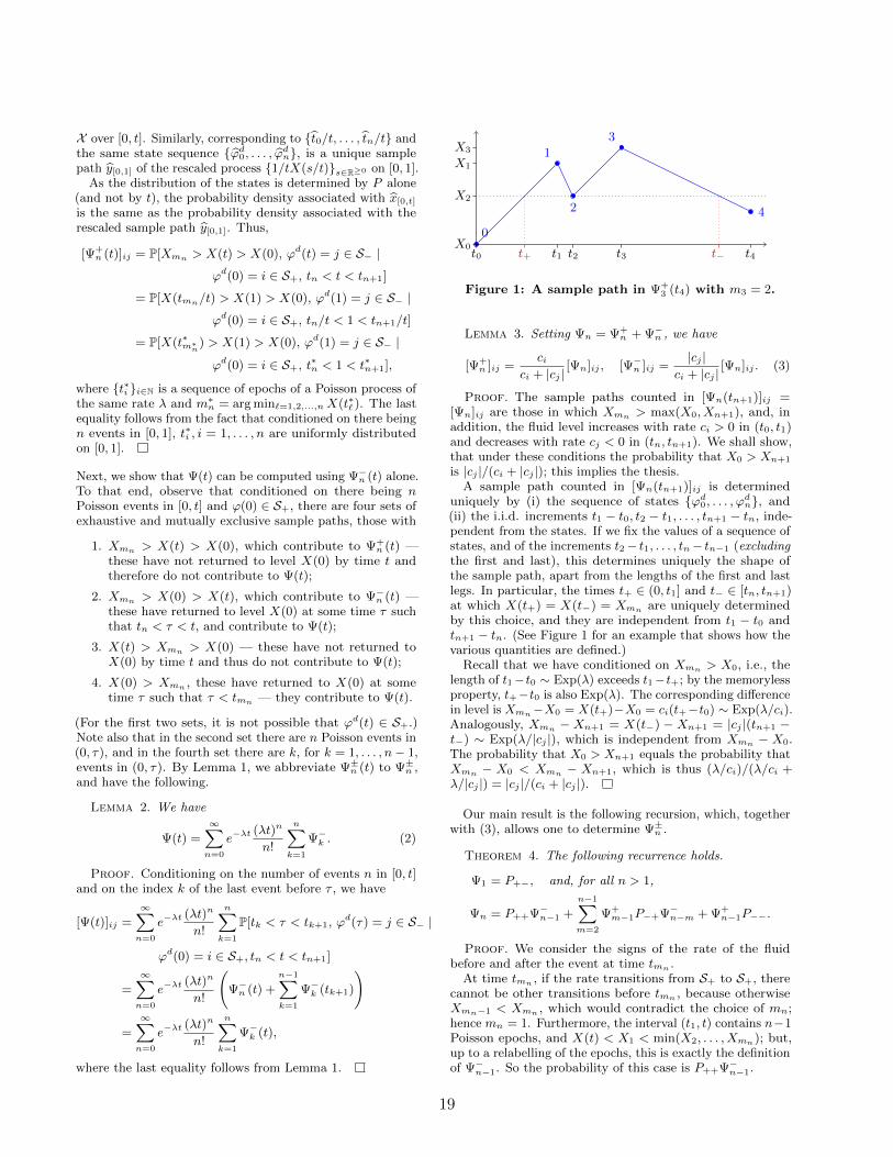
Figure 1: A sample path in Ψ+3 (t4) with m3 = 2.

Lemma 3. Setting Ψn = Ψ+n + Ψ−n , we have

[Ψ+n ]ij =

cici + |cj |

[Ψn]ij , [Ψ−n ]ij =|cj |

ci + |cj |[Ψn]ij . (3)

Proof. The sample paths counted in [Ψn(tn+1)]ij =[Ψn]ij are those in which Xmn > max(X0,Xn+1), and, inaddition, the fluid level increases with rate ci > 0 in (t0, t1)and decreases with rate cj < 0 in (tn, tn+1). We shall show,that under these conditions the probability that X0 > Xn+1

is |cj |/(ci + |cj |); this implies the thesis.A sample path counted in [Ψn(tn+1)]ij is determined

uniquely by (i) the sequence of states ϕd0, . . . , ϕdn, and(ii) the i.i.d. increments t1 − t0, t2 − t1, . . . , tn+1 − tn, inde-pendent from the states. If we fix the values of a sequence ofstates, and of the increments t2− t1, . . . , tn− tn−1 (excludingthe first and last), this determines uniquely the shape ofthe sample path, apart from the lengths of the first and lastlegs. In particular, the times t+ ∈ (0, t1] and t− ∈ [tn, tn+1)at which X(t+) = X(t−) = Xmn are uniquely determinedby this choice, and they are independent from t1 − t0 andtn+1 − tn. (See Figure 1 for an example that shows how thevarious quantities are defined.)

Recall that we have conditioned on Xmn > X0, i.e., thelength of t1−t0 ∼ Exp(λ) exceeds t1−t+; by the memorylessproperty, t+−t0 is also Exp(λ). The corresponding differencein level is Xmn−X0 = X(t+)−X0 = ci(t+−t0) ∼ Exp(λ/ci).Analogously, Xmn −Xn+1 = X(t−) −Xn+1 = |cj |(tn+1 −t−) ∼ Exp(λ/|cj |), which is independent from Xmn − X0.The probability that X0 > Xn+1 equals the probability thatXmn − X0 < Xmn − Xn+1, which is thus (λ/ci)/(λ/ci +λ/|cj |) = |cj |/(ci + |cj |).

Our main result is the following recursion, which, togetherwith (3), allows one to determine Ψ±n .

Theorem 4. The following recurrence holds.

Ψ1 = P+−, and, for all n > 1,

Ψn = P++Ψ−n−1 +

n−1∑

m=2

Ψ+m−1P−+Ψ−n−m + Ψ+

n−1P−−.

Proof. We consider the signs of the rate of the fluidbefore and after the event at time tmn .

At time tmn , if the rate transitions from S+ to S+, therecannot be other transitions before tmn , because otherwiseXmn−1 < Xmn , which would contradict the choice of mn;hence mn = 1. Furthermore, the interval (t1, t) contains n−1Poisson epochs, and X(t) < X1 < min(X2, . . . ,Xmn); but,up to a relabelling of the epochs, this is exactly the definitionof Ψ−n−1. So the probability of this case is P++Ψ−n−1.

19

Symmetrically, if the rate goes from S− to S−, then it mustbe the last, mn = n, otherwise Xmn+1 < Xmn , and it comesafter a path in Ψ+

n−1; this produces the term Ψ+n−1P−−.

In the case the rate goes from from S+ to S−, then therecannot be events before nor after tmn . Hence it must be thecase that mn = n = 1. So in Ψ1 only we have a term P+−,corresponding to the probability of this single transition.

Finally, if the rate changes from S− to S+, then theremust be at least one transition before and after it, so 2 ≤mn ≤ n− 1. In (0, tmn) we have mn − 1 events and observea path in Ψ+

mn−1; in (tmn , t) we have n − mn events and

observe a path in Ψ−n−mn. This produces the summands

Ψ+mn−1P−+Ψ−n−mn

, for each possible value of mn.

3. FINITE APPROXIMATIONIn a numerical algorithm, we need to truncate or approx-

imate the sum (2), which has an infinite number of terms.We propose two different procedures to do this.Algorithm A1. Note thatBn =

∑nk=1 Ψ−k is a non-decreasing

sequence, and limn→∞Bn = Ψ(∞) = Ψ. Generalizing theapproach in [5], whenever n is sufficiently large we can replaceBn with Ψ, which may be computed directly with variousalgorithms (see, e.g., [6]). More specifically, if n′ is the small-

est integer such that (Ψ− Bn′)∑n>n′ e

−λt (λt)nn!

< ε, thenwe can approximate Ψ(t) with

Ψ′(t) =n′∑

n=0

e−λt(λt)n

n!Bn + Ψ

∞∑

n=n′+1

e−λt(λt)n

n!, (4)

with error bounded by

Ψ′(t)−Ψ(t) =∞∑

n=n′+1

(Ψ−Bn)e−λt(λt)n

n!

≤∞∑

n=n′+1

(Ψ−Bn′)e−λt(λt)n

n!< ε.

Algorithm A2. Another truncation strategy consists inswapping the order of summation in (2), obtaining

Ψ(t) =∞∑

k=1

Ψ−k

k−1∑

n=0

e−λt(λt)n

n!.

This sum can be truncated when Ψk is sufficiently small.If we stop the computation of the coefficients at the sameindex n′ as above, we get

Ψ′′(t) =n′∑

k=1

Ψ−k

k−1∑

n=0

e−λt(λt)n

n!≤ Ψ(t). (5)

Note that Ψ′′(t) ≤ Ψ(t) ≤ Ψ′(t), so this method produces anexplicit inclusion interval for each entry of Ψ(t).

The quantities∑k−1n=0 e

−λt (λt)nn!

and∑∞n=n′+1 e

−λt (λt)nn!

are related to the upper and lower incomplete Gamma func-tions by classical identities [4, Eqn. (8.69)], and they can becomputed exactly with the routines included in the mathe-matical libraries of many languages.

4. COMPLEXITY ANALYSISWe compare the complexities of various algorithms to

compute Ψ(t). The primitives required by all of them arelinear algebra operations between matrices whose dimensions

are either |S+| or |S−|. The most general way to boundthe cost of each of these operations is O(N3) floating pointoperations (flops). We shall use this expression in all thecosts in the following.Algorithms A1, A2: computing the recursion in Thm. 4,and then using (4) or (5), respectively, which give approxima-tions from above and from below. They require O(N3(n′)2)flops: we compute n′ steps of the recurrence in Thm. 4, andeach step requires O(n′) linear algebra operations. The valueof n′ required to obtain a prescribed accuracy varies witht. We show in Section 5 (and, especially, in Fig. 2) how thetwo values are related in an example. We often consider A1and A2 together because, once one computes the recursionin Thm. 4, both estimates can be obtained with a minimaltime overhead.Algorithm BST: the algorithm obtained by modifying theapproach suggested in [5] (named after the initials of itsauthors). It is based on filling certain triangular arrays, eachelement of which is a matrix of size |S|× |S−| in our modifiedversion. There are r such arrays, where 1 ≤ r ≤ |S−| is thenumber of distinct negative rates, and each of them has sizeO(n′)2. Filling in each element requires O(1) linear algebraoperations, hence the total complexity of this algorithm isO(N3r(n′)2) flops, which is a factor of r more than A1 orA2.Algorithm LST: the algorithm based on inverse Laplace-Stieltjes transforms (LSTs). Our tests used the Euler al-gorithm in [1] for inversion, which requires evaluating the

transform Ψ(s) in several nodes. The number of nodes rec-ommended in [1] is 2d+1, where d is the number of (decimal)digits of precision required. With ε equal to the machineprecision u, d = 16. Each evaluation was carried out with anumber of steps h of Newton’s method [7, Alg. 4]; each steprequires O(1) linear algebra operations. This gives a totalcost of O(N3dh) flops. Note, h is related to the drift δ of the

fluid by ε = O(δ2h

), due to quadratic convergence results forNewton’s methods.Several points. There is another important factor thatworks against LST. Often, one needs to evaluate Ψ(t) for mdifferent values of t. In A1/A2, the most expensive part iscomputing the recursion; but it is sufficient to do it once,with a truncation criterion n′ determined by the largest of thevalues t. Thus, the total cost to compute Ψ(t1), . . . ,Ψ(tm) isO(N3(n′)2 +N2n′m) flops for A1 and A2, where the secondterms comes from applying (4) and/or (5) m times. ForBST, a similar analysis holds; the complexity is O(N3r(n′)2+N2n′m) flops.

In contrast, we do not know of an established numericalscheme in the literature that allows one to compute inverseLaplace transforms at multiple points, so our best estimatefor LST is m times the cost for one point, i.e., O(N3dhm)flops. This fact makes A1 and A2 a very convenient choicewhen multiple evaluations are required.

A further remark is that a more careful analysis of theN3 term for the linear algebra cost would show that A1, A2,BST scale better than LST when the matrix Q is sparse,or when one among |S+| and |S−| is much smaller than theother.

5. NUMERICAL EXPERIMENTSWe ran some tests to compare the various numerical al-

gorithms. Where not specified otherwise, the truncation

20

Algorithm t = 0.1 t = 1.1 t = 9.9

BST 6.6× 10−16 5.9× 10−16 1.2× 10−15

LST 6.1× 10−11 4.2× 10−11 4.1× 10−11

A1 6.5× 10−16 1.9× 10−16 3.8× 10−16

A2 2.8× 10−16 2.4× 10−16 8.4× 10−16

Table 1: Relative errors obtained with the variousalgorithms in a simple example.

Algorithm t = 0.1 t = 1.1 t = 9.9 t = 15 t = 0:15BST 0.17 0.39 3.54 6.11 6.11LST 0.06 0.09 0.07 0.12 5.49A1 & A2 0.08 0.09 0.26 0.64 0.64n′ 17 47 182 243 243

Table 2: CPU times (seconds) obtained with thevarious algorithms.

threshold ε in A1, A2, and BST is equal to the machineprecision u ≈ 2 · 10−16.Relative errors. We generated a toy model with |S+| =2, |S−| = 3 with the MATLAB instructions

rng(’default’);

T = rand(N); T = T - diag(T*ones(N,1));

C = blkdiag(diag(0.2 * rand(Nplus,1)), ...

-diag(rand(Nminus,1)));

which produced a model with a negative drift of −0.096.We evaluated for each computed value X the relative for-

ward error ‖X−X‖∞/‖X‖∞. Here X is an ‘exact’ referencevalue obtained by running both LST and A1 with higherworking precision, as well as a higher number of nodes forLST, and checking that their results coincide up to the ma-chine precision u.

Table 1 confirms that LST (with normal working precisionand the default number of nodes d = 16) can obtain only anaccuracy of the order of 10−11. These results are consistentwith the theory in [1, Sect. 7], which predicts an accuracy (forwell-behaved functions) of 0.6d decimal digits when workingwith 2d+ 1 nodes and d decimal digits of precision. Furthertests show that this is the typical behaviour, at least for smallvalues of |S|, although computing these reference values isextremely slow.Running times. We generated a more challenging test,with the same code but |S+| = 10, |S−| = 11. Table 2 showsthe CPU times obtained for several values of t and, in the lastcolumn, for when 100 values equispaced in [0, 15] are com-puted simultaneously. The results show that LST requires aconstant time to compute each time sample, irrespective oft, while the other algorithms get slower as t increases. Onthe other hand, these algorithms can compute the 100 timesamples of Ψ(t) basically with no overhead w.r.t. the costof computing the one with the largest t. This confirms thetheory in Section 4.

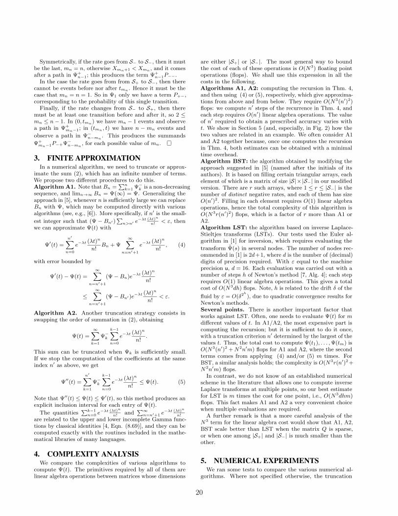
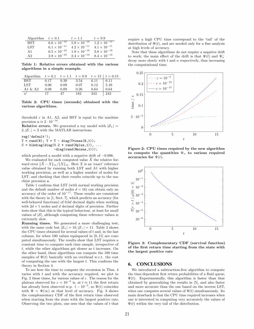
To see how the time to compute the recursion in Thm. 4varies with t and with the accuracy required, we plot inFig. 2 these times, for various values of ε. The reason for theplateau observed for ε = 10−5 is, at t ≈ 11 the first returnhas already been observed w.p. 1− 10−5, so Ψ(t) coincideswith Ψ = Ψ(∞) at that level of accuracy. Fig. 3 showsthe complementary CDF of the first return time observedwhen starting from the state with the largest positive rate.Observing the two plots, one sees that the values of t that

require a high CPU time correspond to the ‘tail’ of thedistribution of Ψ(t), and are needed only for a fine analysisat high levels of accuracy.

Note that these algorithms do not require a negative driftto work; the main effect of the drift is that Ψ(t) and Ψ−ndecay more slowly with t and n respectively, thus increasingthe computational time.

0 5 10 15

0

5 · 10−2

0.1

0.15

0.2

0.25

t

tim

e/s

ε = 10−5

ε = 10−10

ε = 10−15

Figure 2: CPU times required by the new algorithmto compute the quantities Ψn to various requiredaccuracies for Ψ(t).

0 5 10 15

10−6

10−5

10−4

10−3

10−2

10−1

100

t

P[τ>t|ϕ

(0)

=1]

Figure 3: Complementary CDF (survival function)of the first return time starting from the state withthe largest positive rate

6. CONCLUSIONSWe introduced a subtraction-free algorithm to compute

the time-dependent first return probabilities of a fluid queue,Ψ(t). Experimentally, this algorithm is faster than thatobtained by generalizing the results in [5], and also fasterand more accurate than the one based on the inverse LST,when one computes several values of Ψ(t) simultaneously. Itsmain drawback is that the CPU time required increases whenone is interested in computing very accurately the values ofΨ(t) within the very tail of the distribution.

21

7. REFERENCES[1] J. Abate and W. Whitt. A unified framework for

numerically inverting Laplace transforms. INFORMS J.Comput., 18(4):408–421, 2006.

[2] S. Ahn and V. Ramaswami. Efficient algorithms fortransient analysis of stochastic fluid flow models. J.Appl. Probab., 42(2):531–549, 2005.

[3] A. S. Alfa, J. Xue, and Q. Ye. Accurate computation ofthe smallest eigenvalue of a diagonally dominantM -matrix. Math. Comp., 71(237):217–236, 2002.

[4] G. B. Arfken and H. J. Weber. Mathematical methodsfor physicists. Elsevier Academic press, sixthinternational edition, 2005.

[5] N. Barbot, B. Sericola, and M. Telek. Distribution ofbusy period in stochastic fluid models. Stoch. Models,17(4):407–427, 2001.

[6] N. G. Bean, M. M. O’Reilly, and P. G. Taylor.Algorithms for return probabilities for stochastic fluidflows. Stoch. Models, 21(1):149–184, 2005.

[7] N. G. Bean, M. M. O’Reilly, and P. G. Taylor.Algorithms for the Laplace-Stieltjes transforms of firstreturn times for stochastic fluid flows. Methodol.Comput. Appl. Probab., 10(3):381–408, 2008.

[8] G. T. Nguyen and F. Poloni. Componentwise accuratefluid queue computations using doubling algorithms.Numer. Math., 130(4):763–792, 2015.

[9] C. A. O’Cinneide. Entrywise perturbation theory anderror analysis for Markov chains. Numer. Math.,65(1):109–120, 1993.

22

MATRIX ANALYTIC METHODS FOR REFLECTED RANDOMWALKS WITH STOCHASTIC RESTARTS

Dario A. BiniDipartmento di Matematica,

Università di PisaL.go Bruno Pontecorvo, 5

56127, Pisa, [email protected]

Stefano MasseiEPFL

MA B2 515 (Bâtiment MA)CH-1015 Lausanne,

[email protected]

Beatrice MeiniDipartmento di Matematica,

Università di PisaL.go Bruno Pontecorvo, 5

56127, Pisa, [email protected]

Leonardo RobolISTI

Area della ricerca CNRVia G. Moruzzi, 156124, Pisa, Italy

[email protected]

ABSTRACTWe consider some Markov processes involving infinite statespaces, e.g., Quasi-Birth-and-Death (QBD) on N or N2. Of-ten their transition probability matrices have Toeplitz orblock Toeplitz structure, and the boundary conditions areencoded by low-rank corrections with finite support. Findingtheir steady state probability distribution can be recasted tofinding minimal solutions to the quadratic matrix equation

AX2 + BX + C = X,

where the matrices A,B,C are obtained from the blocks ofthe multilevel Toeplitz matrix. The state-of-the-art algo-rithms to solve these equations require to perform matrixoperations involving these matrices. When the Markov pro-cess is defined on N2, the matrices A,B,C are semi-infinite.Recently, a computational framework for handling these prob-lems without truncating the dimension of the state spacehas been proposed in [2]. This is achieved by approximatingthis kind of matrices as the sum of a banded semi-infiniteToeplitz plus a low-rank correction with finite support.

We propose an extension of this framework which allows todeal with more general situations such as processes involvingrestart events, where the process can move to level (or phase)0 at any moment with a certain positive probability. This ismotivated by the need for modeling processes that can incurin unexpected failures like computer system reboots. Alge-braically, this gives rise to corrections with infinite supportthat can not be treated using the tools currently availablein the literature. We present a theoretical analysis of anenriched space that, combined with appropriate algorithms,enables the numerical treatment of these problems. We



demonstrate that the new approach considerably improvesthe method proposed in [2] as well, since there are caseswhere the coefficients A,B,C live in the space describedthere, but the solution X cannot be approximated withoutconsidering low-rank corrections with infinite support [1].We show that this class of problem, previously numericalintractable, can now be handled in this framework.

We test our implementation on some case studies thatconfirm the applicability of the method.

1. REFERENCES[1] D. Bini, S. Massei, B. Meini, and L. Robol. On

quadratic matrix equations with infinite size coefficientsencountered in qbd stochastic processes. NumericalLinear Algebra with Applications, 2018.

[2] D. A. Bini, S. Massei, and B. Meini. Semi-InfiniteQuasi-Toeplitz Matrices with Applications to QBDStochastic Processes. Mathematics of Computation,2018.

23

Extinction in lower Hessenberg branching processes withcountably many types

Peter BraunsteinsThe University of Melbourne

Grattan Street, Parkville, Victoria, [email protected]

Sophie HautphenneThe University of Melbourne

Grattan Street, Parkville, Victoria, [email protected]

ABSTRACTWe consider a class of branching processes with countablymany types which we refer to as Lower Hessenberg branchingprocesses. These are multitype Galton-Watson processes withtypeset X = 0, 1, 2, . . . , in which individuals of type i maygive birth to offspring of type j ≤ i+ 1 only. For this class ofprocesses, we study the set S of fixed points of the progenygenerating function. In particular, we highlight the existenceof a continuum of fixed points whose minimum is the globalextinction probability vector q and whose maximum is thepartial extinction probability vector q. In the case whereq = 1, we derive a global extinction criterion which holdsunder second moment conditions, and when q < 1 we developnecessary and sufficient conditions for q = q.



24

The probabilities of extinction in a branching random walkon a strip

Peter BraunsteinsThe University of Melbourne

MelbourneAustralia

[email protected]

Sophie HautphenneThe University of Melbourne

MelbourneAustralia

[email protected]

ABSTRACTWe consider a class of multitype Galton-Watson branchingprocesses with countably infinite type set X whose meanprogeny matrices have a block lower Hessenberg form. Forthese processes, we derive partial and global extinction cri-teria. Our approach involves embedding a finite-type explo-sive Galton-Watson process in a varying environment in theoriginal infinite-type process, and then establishing asymp-totic relationships between the two processes. We study theprobability of extinction in sets of types A ⊆ X , q(A). Inparticular, we develop conditions for q(A) to be differentfrom the global and partial extinction probability vectors.We present an iterative method to compute the vectors q(A),and investigate their location in the set of fixed points of theprogeny generating vector.

1. REFERENCES[1] P. Braunsteins, G. Decrouez, and S. Hautphenne. A

pathwise approach to the extinction of branchingprocesses with countably many types. StochasticProcesses and their Applications, 2018. In Press.

[2] P. Braunsteins and S. Hautphenne. Extinction in lowerhessenberg branching processes with countably manytypes. arXiv:1706.02919, 2018.

[3] P. Braunsteins and S. Hautphenne. The probabilities ofextinction in a branching random walk on a strip.arXiv:1805.07634, 2018.

[4] S. Hautphenne, G. Latouche, and G. Nguyen. Extinctionprobabilities of branching processes with countablyinfinitely many types. Advances in Applied Probability,45(4):1068–1082, 2013.



25

On Fisher Information of Some Functions of Phase TypeVariates

Pavithra Celeste RDepartment of Mathematics

Indian Institute of SpaceScience and Technology

[email protected]

T. G. DeepakDepartment of Mathematics

Indian Institute of SpaceScience and Technology

[email protected]

ABSTRACTBladt et.al. [2] introduced a method for obtaining FIM(FisherInformation Marix) for PH(Phase Type) class using theExpectation- Maximisation (EM) algorithm. In this article,we attempt to find out the Fisher Information for somefunctions of PH variates. We discuss the following cases : (i)when the function g(X), of the PH variate X, is differentiablefor all X = x and either the derivative at x is strictly positiveor negative, (ii) when the derivative of g is continuous andnon zero for all but finite number of values of x and forevery real number y, there exists n = n(y) inverses and, (iii)when Y = g(X) and g is invertible only in a finite intervaland at each point y the function is having countable numberof inverses. The FIM for the finite support PH variates,which comes under case (iii), introduced by Ramaswami andViswanath [7], is computed using the EM algorithm.

Keywords: Finite support phase type distributions;Fisher information; EM algorithm; Functions of PH vari-ates .

1. INTRODUCTIONPhase type (PH) distributions introduced by Neuts [5]

form a dense family of distributions (in the metric of weakconvergence of distributions) on [0,∞) and have found lotof applications in the area of applied probability. A PHdistribution can be regarded as the distribution of the timeuntil absorption in a finite state Markov chain with oneabsorbing state into which absorption is certain. In the recentpast, many research papers have been appeared to study, themodels which are governed by PH distributed time. Apartfrom their denseness property that makes them versatile asmodels, there are many other motivations for using PHdistributions in statistical models. The most importantones come from their connection with Markov chains andmatrix theory. While the former is offering much simplicityin various conditioning arguments occurred in the modelanalysis, the latter is helping us to develop more accurate



and faster algorithms that make many models involving PHdistributions computationally tractable.

Phase type distributions, however, can be used for mod-elling only non-negative random variables, and they havean infinite support. But, in practice, there are many ran-dom variables for which the distributions have finite support.Even though, theoretically, the denseness property of thePH class allow us to fit such distributions by a suitable PHdistribution, it may require a representation of large orderso that practically the fit may not render a realistic approx-imation. In order to cater to the needs of this situation,Ramaswami and Viswanath [7] introduced a new class ofdistributions derived from PH distributions called, phasetype distributions with finite support (FSPH). Since thesedistributions are also based on phase type distributions, theybear a strong connection to Markov chains. Their densitiesare of the matrix exponential type giving thereby the abilityto bring to bear all the tools of matrix computations.

Fisher information or more commonly called Fisher infor-mation matrix (FIM) plays a key role in uncertainty calcula-tion and in other aspects of estimation for a wide range ofstatistical applications. It essentially describes the amountof information that the data provide about unknown parame-ters. The expected FIM, that is the expectation of the squareof the gradient of the incomplete data log-likelihood functionsat the maximum likelihood estimates (MLEs), can be usedto calculate the Cramer-Rao lower bound and asymptoticdistribution of the MLE. The role of FIM in the computationof the asymptotic distribution of the MLE enable us to use iteffectively in testing of hypothesis and in the construction ofconfidence regions for the unknown parameters. In additionto compute the Fisher information contained in the sampleobservations assumed by a single variate, the same can becomputed for the sample taken from a process.

The expectation-maximization (EM) algorithm introducedby Dempster, Laird and Rubin [3] is a well-known methodto compute the MLE iteratively from the observed data.It is applied to problems in which the observed data isincomplete or the log-likelihood function of the observeddata is too difficult to be solved to get the MLE directlyfrom it. It provides a sequence of results obtained fromthe simple complete data log-likelihood function, and henceavoids calculations from the complicated incomplete data log-likelihood function. One of the major criticisms of the EMapproach was that it cannot be directly used to obtain theFIM for the observed data since the EM algorithm does notautomatically produce an estimate of the covariance matrix

26

of the MLE. However, Oakes [6] provided a simple explicitformula for the matrix of second derivatives of the criterionfunction (the conditional expectation of the complete datalog-likelihood given the observed data) invoked by the EMalgorithm.

Estimation and statistical inference for PH distributionsare of considerable importance when taking into consider itsrole in different areas of application. Asmussen, Nerman, andOlsson [1] was the first to develop a general approach to MLestimation of continuous PH distributions. Bladt, Esparza,and Nielsen [2] suggested an alternative method of calculatingmatrix exponentials and related integrals, appearing in the E-step in the EM algorithm, in order to speed up the executionof the algorithm considerably well for small and mediumsized data sets. Apart from this, the main contributionsof Bladt, Esparza, and Nielsen [2] are that of proposingmethods for calculating the FIM for discrete and continuousPH distributions using formulae that are related to both EMalgorithm and the Newton-Raphson approach.

In this paper, we discuss the computation of FIM of somefunctions of PH variates by the EM approach. We follow themethod adopted by Bladt, Esparza, and Nielsen [2] - wherethey considered FIM for PH class - for computing FIM ofsome functions of PH variates .

2. FIMWe consider the following three types of functions of a PH

variate X.

2.1 Case 1Let the function Y = g(X) be differentiable for all X = x

and the derivative g′ at x is either strictly positive or negative.In this case the function g will be invertible. So, if we aregiven n observations y1, y2, . . . , yn from Y , then by taking theinverses of these observations i.e, g−1(y1), g−1(y2), . . . , g−1(yn),we get n observations from g−1(Y ) = X, a PH variate. Hencewe can compute the FIM of Y using that of X, which isalready known. For example, the FIM of logPH distribu-tion, introduced by Ahn et. al. [8], can be computed in thismanner.

2.2 Case 2Let the derivative of g be continuous and non zero for all

but finite number of values of x and for every real numberthere exist a finite number of inverse values.i.e, for everyreal number y, there exist a positive integer n = n(y) andreal numbers x1, x2, . . . , xn such that, g[xk] = y, g′[xk] 6=0, k = 1, 2, . . . , n(y).This case can be illustrated with the example, Y = |X − k|where k is any positive real number.

2.3 Case 3Here we consider the case when Y = g(X), where g is, in

general, not an invertible function. Assume that in a finiteinterval g is invertible and at each point y, the function ishaving countable number of inverses, which are given byh(y) + l(n), n = 0, 1, 2, . . . where h is the inverse of g in thefinite interval and l is a linear function of n. So once we aregiven a sample from Y , using the relation X = h(Y ) + l(n)we can obtain observations from a PH variate. Also, if F is

the distribution function of X, then that of Y is,

F (y) =∞∑

n=0

[F (h(y) + l(n))− F (l(n))].

Now using this distribution function and the MLE of thePH−variate X, we obtain the MLE as well as the FIM ofY.

As an example, we have considered two functions of PHvariates namely FSPH variate and sine function. In Oakes[6],the FIM is given as,

∂2L(θ; y)

∂θ2=

∂2Q(θ/θ)

∂θ2+∂2Q(θ/θ)

∂θ∂θ

θ=θ

where Q(θ/θ) = Eθ(lf (θ;x)/y

).

For finding the FIM of an FSPH variate of order p, letθ = (α1, α2, · · ·αp−1, t1, T12, · · ·T1p, T21, t2, T23 · · ·T2p, · · ·Tp1, Tp2 · · ·Tp,p−1, tp)be the parameter vector of order p−1+p2 for the FSPH1(α, T )distribution. Note that here we take αp = 1−∑p−1

j=1 αj and

Tii = −∑pj=1j 6=i

Tij − ti. Since the FSPH distribution is be-

ing derived from the PH distribution, from the likelihoodfunction of the latter, we get,

Q(θ/θ) =

p∑

i=1

log(αi)n∑

k=1

Bik

+

p∑

i=1

p∑

j=1j 6=i

n∑

k=1

log(Tij)Nijk

−p∑

i=1

p∑

j=1j 6=i

n∑

k=1

TijZik

+

p∑

i=1

n∑

k=1

log(ti)Nik

−p∑

i=1

n∑

k=1

tizik

where Bik, Ni

k, Nij

kand Zi

kare the estimates of the suffi-

cient statistics Bi, Ni, Nij and Zi respectively related to thekth sample observation, and Bi, Ni, Nij and Zi are given by,

• Bi, the number of trajectories that start in phase i,i = 1, 2, · · · , p.

• Ni, the number of trajectories for which absorptionoccurs from phase i, i = 1, 2, · · · , p.

• Nij , the number of transitions that occur from phase ito phase j, 1 ≤ i, j ≤ p, i 6= j.

• Zi, the total sojourn time in phase i for all the ntrajectories combined, for i = 1, 2, · · · , p.

Then by substituting α =∑p−1j=1 αje

Tj +

(1−∑p−1

j=1 αj)eTp

and using the FIM of PH distribution, we get the elements ofthe FIM for FSPH1(α, T ) distribution of order p as follows:For i, j = 1, 2, · · · p− 1, the (i, j)th element is given by

∂Ui∂αj

− ∂Up∂αj

;

for m = 1, 2, · · · p−1 and i, j = 1, 2 · · · p, the (ip−1 + j,m)th

element is given by

∂Um∂Tij

− ∂Up∂Tij

if i 6= j,∂Um∂ti

− ∂Up∂ti

if i = j;

27

the (m, ip− 1 + j)th element is given by

∂Vij∂αm

− ∂Vii∂αm

if i 6= j,∂Wi

∂αm− ∂Vii∂αm

if i = j;

and for i, j,m, n = 1, 2 · · · p, the (ip− 1 + j,mp− 1 + n)th

element is given by

∂Vij∂Tmn

− ∂Vii∂Tmn

if i 6= j,m 6= n,∂Vij∂tm

− ∂Vii∂tm

if i 6= j,m = n,

∂Wi

∂Tmn− ∂Vii∂Tmn

if i = j,m 6= n,∂Wi

∂tm− ∂Vii∂tm

if i = j,m = n,

where,

Ui =∑nk=1

e′ie

Tyk (I−eT )−1t

f(yk)

Wi =∑nk=1

αeTyk (I−eT )−1eif(yk)

Si = −∑pj=1j 6=i

Tij − ti

and Vij =∑nk=1

e′jM∗(yk,α,T )ei

f(yk),

with,

M∗(y, α, T ) = (I − eT )−1 M(y, α, T ) + (I − eT )−1

M(1, α, T ) (I − eT )−1eTy

and M(y, α, T ) =

∫ y

0

eT (y−u) tαeTu du.

As an another example we have considered the case ofY = sinX, where X is a PH(α, T ) variate, in which case weget the distribution function of Y as,

F (y) =αT−1(I − e2πT )−1

[eπT (eπT − e− sin−1 yT )+

esin−1 yT − I

]tδ0≤y≤1 +

αT−1(I − e2πT )−1

eπT[e(π−sin−1 y)T − esin−1(−y)T

]tδ−1≤y≤0

where δ is the indicator function.Proceeding as in the above case, we can compute the FIMof Y.

The Fisher information matrix is widely used in optimalexperimental design, machine learning, physics, computa-tional neuroscience etc. It is used in the formulation of teststatistics as well as finding the confidence region of parame-ters under consideration. The inverse of the FIM gives theasymptotic variances and covariances of the maximum likeli-hood estimates of the parameters. The FIM, in general, isnot invertible and the invertibility has to be verified for eachmodel. Since the same phase type distribution has differentrepresentations, we can expect the non-singularity for therepresentation with minimum number of parameters. Thethree cases, that are discussed in this paper covers almostall classes of distributions which can be obtained from theclass of PH- distributions. Many of them find applicationsin various fields including insurance and finance. For ex-ample, LogPH class distributions exhibits a heavy tail andhas some nice tail properties that are well aligned with theextreme value theory. Since fitting heavy tailed loss datawith parametric distributions being an important analyticaltask in the insurance field, LogPH, which can fit the wholedata in a straightforward manner plays an important rolein insurance field. In addition, some classes of distributions,which come under the above discussed cases, have denseness

properties (denseness of FSPH and LogPH are proven). Sothe statistical inference of those classes can offer the proper-ties of rich classes of distributions without separate analyses.Hence the parameter estimation and the computation of FIMplay an important role in the statistical inference of manydistributions which are having practical applications.

3. REFERENCES[1] S. Asmussen,O. Nerman and M. Olsson. Fitting

phase-type distributions via the EM algorithm. Scand. J.Statist. 1996, 23, 419-441.

[2] M. Bladt, L. J. Esparza and B. F. Nielsen. Fisherinformation and statistical inference for phase-typedistributions. J. Appl. Prob. Spec. 2011, 48A, 277-293.

[3] A. P. Dempster,N. M. Laird and D. B. Rubin. Maximumlikelihood from incomplete data via the EM algorithm.J. R. Statis. Soc.: Series B (Methodological). 1977,39,1-38.

[4] G. Latouche and V. Ramaswami. Introduction to MatrixAnalytic Methods in Stochastic Modeling , SIAM & ASA:Philadelphia, 1999.

[5] M. F. Neuts. Matrix Geometric Solutions in StochasticModels, Johns Hopkins University Press: Baltimore &London, 1981.

[6] D. Oakes. Direct calculation of the information matrixvia the EM. J. R. Statis. Soc.: Series B (StatisticalMethodology). 1999, 61(2), 479-482.

[7] V. Ramaswami, and N. C.Viswanath. Phase typedistributions with finite support. Stoch. Models. 2014,30, 576-597.

[8] Soohan Ahn, Joseph H.T Kim and VaidyanathanRamaswami. A new class of models for heavy taileddistributions in finance and insurance risk. Insurance:Mathematics and Economics. 2012, 51, 43-52

28

Model for the evolution of the family of gene duplicates

Jiahao DiaoUniversity of Tasmania

Churchill AvenueHobart, Tasmania

[email protected]

Tristan L. StarkTemple University1900 N 12th StreetPhiladelphia, USA

[email protected]

David A. LiberlesTemple University1900 N 12th StreetPhiladelphia, USA

[email protected]łgorzata M. O’Reilly ∗†

University of TasmaniaChurchill AvenueHobart, Tasmania

[email protected]

Barbara R. Holland ∗


[email protected]

ABSTRACTConsider a Markov model for the evolution of the family ofgenes proposed in [1, Section 10], in which the state (n,m)records the number copies n = 0, 1, 2, . . ., and the number ofredundant copies m = 0, 1, , . . . , n of a gene in the family. Byredundant copies we mean copies whose loss will not result inthe loss of the functions of the gene when these are presevedby some other genes in the family.

The transition rates between the state of the Markov modelin [1, Section 10] depend on the following key processes: du-plication of a gene; loss of one copy of a gene; one copyacquiring a new function (neofunctionalisation); and a lossof some regulatory region in one of the genes which leads toa number of genes required to fulfill some function (subfunc-tionalisation).

The aim of this work is to develop suitable expressions forthe transition rates function. As an initial inspiration of ouranalysis, we consider a Markov model with a more detailedstate, represented as a matrix, where rows corresponds to thevarious genes in the family, and columns to their functions.That is, state is a binary matrix A = [Aij ]i=1,...,M ;j=1,...,Z ,where M is the number of genes in the family, and Z thenumber of functions, such that Aij = 1 when function j isperformed by some regulatory region of gene i, and 0 other-wise.

∗We would like to thank the Australian Research Coun-cil for funding this research through Discovery ProjectDP180100352.†Australian Research Council Centre of Excellence for Math-ematical and Statistical Frontiers.



Although we suspect that the model with the detailedrepresentation will not be tractable for developing analyticsolutions (except in very small cases) we propose to use itas a simulation model to give insight into suitable transitionrates in the reduced state space representation.

1. REFERENCES[1] A. I. Teufel, J. Zhao, M. O’Reilly, L. Liu, and D. A.

Liberles. On mechanistic modeling of gene contentevolution: birth-death models and mechanisms of genebirth and gene retention. Computation, 2(3):112–130,2014.

29

Characterization of the Boundary of the Set ofMatrix-Exponential Distributions with Only Real Poles

Qi-Ming HeDepartment of Management

Sciences, University ofWaterloo

200 University Avenue WestWaterloo, Ontario, Canada

N2L [email protected]

Mark FackrellSchool of Mathematics and

StatisticsUniversity of Melbourne

Melbourne, Vic 3010, [email protected]

Peter TaylorSchool of Mathematics and

StatisticsUniversity of Melbourne

Melbourne, Vic 3010, [email protected]

ABSTRACTWe study the boundary of the set of matrix-exponential dis-tributions with m real poles. We show that the boundaryconsists of three parts: two parts in some lower dimensionalspaces and a curved part. The curved part is characterizedas the union of convex hulls of solutions from m− 2 curveseach generated by three Coxian distributions. The charac-terization of the boundary leads to algorithms for construct-ing the set of matrix-exponential distributions.

1. REFERENCES[1] Bean N, Fackrell M, Taylor P (2008) Characterization

of matrix-exponential distributions. Stochastic Models24 (3): 339-363.

[2] Dehon M, Latouche G (1982) A geometricinterpretation of the relations between the exponentialand generalized Erlang distributions. Advances inApplied Probability 14: 885-897.

[3] Fackrell M (2003) Characterization ofMatrix-exponential Distributions. PhD thesis, Schoolof Applied Mathematics, University of Adelaide,South Australia, 2003. Available athttp://thesis.library.adelaide.edu.au/public/adt-SUA20051207.123257/.

[4] Neuts MF (1981) Matrix-Geometric Solutions inStochastic Models: An Algorithmic Approach. TheJohn Hopkins University Press: Baltimore.

[5] O’Cinneide CA (1990) Characterization of phase-typedistributions. Stochastic Models 6: 1-57.



30

Markovian decision-support model for patient-to-wardassignment problem in a random environment

Mojtaba Heydar †University of Tasmania

TAS 7001, [email protected]

Małgorzata M. O’Reilly ∗†University of Tasmania


ABSTRACTThe purpose of this research is to model the decision makingprocess in a hospital in which patients are allocated to bedsin different wards, according to their needs, priorities, aswell as availability of the resources. The problem analysedhere is a generalisation of the advanced patient admissionscheduling (APAS) problem studied in [1, 2, 6], in which pa-tients are admitted and alocated to the hospital capacitatedresources [2] over some planning horizon.

We construct a Markov Decision Process (MDP), in which,at the start of the planning period, arrived patients are as-signed to suitable wards in a manner that optimises theperformance measures of interest. We build on the MDPmodel in [7], in which decisions are made at the time of arrivalor departure of a patient. Here, we assume that the deci-sions are made at the start of the time period of some fixedlength, and so the allocation involves several arrived patients.

Assume that the information about the system at the startof the planning period is given as state s = ([nk,i]K×I , [qi]1×I),where nk,i is the number of type-i patients in ward k, withi ∈ I, k ∈ K, and qi is the number of newly arrived type-ipatients (or the expected number of type-i patients to arriveduring the current period), who are yet to be assigned to thewards.

Here, I = 1, 2, . . . , I is the set of all patient types, wherea type may correspond to the medical needs of the patient,their priority, their age, gender, and other relevant features.We assume that the set I is ordered according to the priori-ties, so that 1 and I represents the least and the most severepatients, respectively. Furthermore, K is the set of the wardsin the hospital system. There are Bk beds in ward k ∈ K.

∗We would like to thank the Australian Research Council forfunding this research through Linkage Project LP140100152.†ARC Centre of Excellence for Mathematical and StatisticalFrontiers.



Suppose that type-i patients arrive according to a Poissonprocess with the rate λi. Let Qi(t) be the random variablerecording the number of arrivals of type-i patients during thetime period of length t. The distribution of Qi(t) is Poisson,Qi(t) ∼ Poi(λit).

The newly assigned type-i patient will stay in ward k forthe duration of time LoSk,i, referred to as the length ofstay, according to some discrete Phase-type distribution [3,

4], PH(γ(k,i),P(k,i)). Let Zk,i(t) be the random variablerecording the number of departures of type-i patients fromward k during the time period of length t. The distributionof Zk,i(t) is binomial, Zk,i(t) ∼ Bin(nk,i, pk,i(t)), where

pk,i(t) = Pr(LOSk,i ≤ t) = 1− γ(k,i)(P(k,i)

)t1,

for all t = 0, 1, 2, . . ., where 1 is a column vector of ones ofappropriate size.

After observing state s = ([nk,i]K×I , [qi]1×I), a decisiona = ([xk,i]K×I , [yk,`,i]K×K×I) is made about where to assignthe patients, which involves assigning xk,i type-i patients toward k, and transfering yk,`,i type-i patients from ward k to `.The resulting post-decision state is some s = ([nk,i]K×I),with

nk,i = nk,i + xk,i +∑

k∈Kyk,`,i −

∑

`∈Kyk,`,i.

Following the decision a, the process transitions from state sto some state s′ =

([n′k,i]K×I , [q

′i]1×I

)with n′k,i = nk,i−zk,i,

according to the probability given by

Prs′| (s, a) =∏

i

Pr(Qi(t) = q′i)∏

k,i

Pr(Zk,i(t) = zk,i).

The above model describes the evolution of the systemthat depends on decision making process as well as randomarrivals and departures in a given time period of length t.We formulate suitable value function and constraints, andconsider the corresponding infinite-horizon MDP, in whichthe aim is to optimise the long-run discounted total meancost, given discount factor α.

Since solving large-scale infinite-horizon MDPs is a chal-lenging task, we consider suitable approximation techniques,such as Approximate Dynamic Programming (ADP)[5], inorder to find an approximation that represent the valuefunction of the MDP.

31

1. REFERENCES[1] Y. Gocgun and M. L. Puterman. Dynamic scheduling

with due dates and time windows: an application tochemotherapy patient appointment booking. Health caremanagement science, 17(1):60–76, 2014.

[2] P. J. Hulshof, M. R. Mes, R. J. Boucherie, and E. W.Hans. Patient admission planning using approximatedynamic programming. Flexible services andmanufacturing journal, 28(1-2):30–61, 2016.

[3] G. Latouche and V. Ramaswami. Introduction to MatrixAnalytic Methods in Stochastic Modelling, 1st edition.Chapter 2: PH Distributions. ASA SIAM, 1999.

[4] M. F. Neuts. Matrix-Geometric Solutions in StochasticModels: an Algorithmic Approach, Chapter 2:Probability Distributions of Phase Type. DoverPublications Inc., 1981.

[5] W. B. Powell. Approximate Dynamic Programming:Solving the curses of dimensionality. John Wiley & Sons,2007.

[6] S. Samiedaluie, B. Kucukyazici, V. Verter, and D. Zhang.Managing patient admissions in a neurology ward.Operations Research, 65(3):635–656, May-June 2017.

[7] E. Trainer, M. M. O’Reilly, M. Fackrell, P. G. Taylor,A. Tirdad, and M. Heydar. Stochastic model forpatient-bed asignment problem with random arrivalsand departures. In preparation.

32

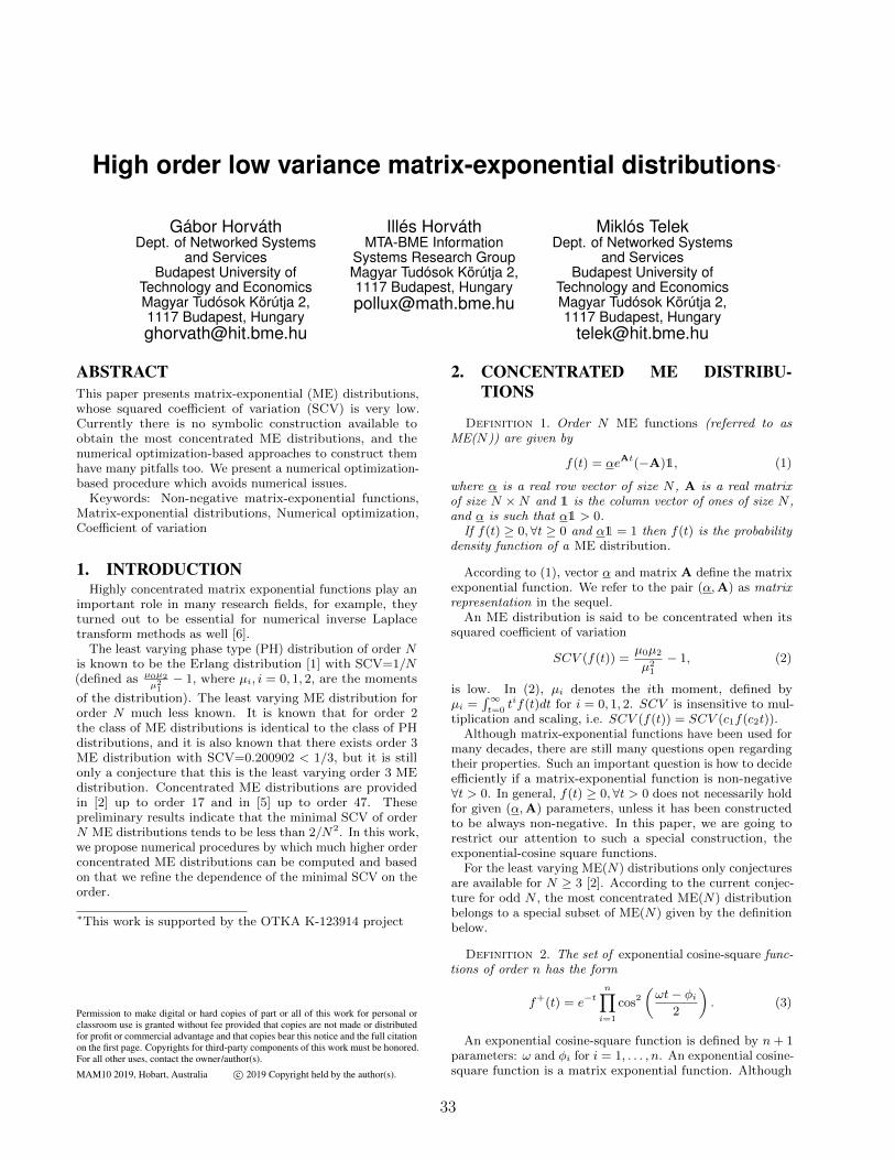
High order low variance matrix-exponential distributions∗

Gábor HorváthDept. of Networked Systems

and ServicesBudapest University of

Technology and EconomicsMagyar Tudósok Körútja 2,1117 Budapest, [email protected]

Illés HorváthMTA-BME Information

Systems Research GroupMagyar Tudósok Körútja 2,1117 Budapest, [email protected]

Miklós TelekDept. of Networked Systems

and ServicesBudapest University of

Technology and EconomicsMagyar Tudósok Körútja 2,1117 Budapest, Hungary

[email protected]

ABSTRACTThis paper presents matrix-exponential (ME) distributions,whose squared coefficient of variation (SCV) is very low.Currently there is no symbolic construction available toobtain the most concentrated ME distributions, and thenumerical optimization-based approaches to construct themhave many pitfalls too. We present a numerical optimization-based procedure which avoids numerical issues.

Keywords: Non-negative matrix-exponential functions,Matrix-exponential distributions, Numerical optimization,Coefficient of variation

1. INTRODUCTIONHighly concentrated matrix exponential functions play an

important role in many research fields, for example, theyturned out to be essential for numerical inverse Laplacetransform methods as well [6].

The least varying phase type (PH) distribution of order Nis known to be the Erlang distribution [1] with SCV=1/N(defined as µ0µ2

µ21− 1, where µi, i = 0, 1, 2, are the moments

of the distribution). The least varying ME distribution fororder N much less known. It is known that for order 2the class of ME distributions is identical to the class of PHdistributions, and it is also known that there exists order 3ME distribution with SCV=0.200902 < 1/3, but it is stillonly a conjecture that this is the least varying order 3 MEdistribution. Concentrated ME distributions are providedin [2] up to order 17 and in [5] up to order 47. Thesepreliminary results indicate that the minimal SCV of orderN ME distributions tends to be less than 2/N2. In this work,we propose numerical procedures by which much higher orderconcentrated ME distributions can be computed and basedon that we refine the dependence of the minimal SCV on theorder.

∗This work is supported by the OTKA K-123914 project


MAM10 2019, Hobart, Australia c© 2019 Copyright held by the author(s).

2. CONCENTRATED ME DISTRIBU-TIONS

Definition 1. Order N ME functions (referred to asME(N)) are given by

f(t) = αeAt(−A)1, (1)

where α is a real row vector of size N , A is a real matrixof size N ×N and 1 is the column vector of ones of size N ,and α is such that α1 > 0.

If f(t) ≥ 0, ∀t ≥ 0 and α1 = 1 then f(t) is the probabilitydensity function of a ME distribution.

According to (1), vector α and matrix A define the matrixexponential function. We refer to the pair (α,A) as matrixrepresentation in the sequel.

An ME distribution is said to be concentrated when itssquared coefficient of variation

SCV (f(t)) =µ0µ2

µ21

− 1, (2)

is low. In (2), µi denotes the ith moment, defined byµi =

∫∞t=0

tif(t)dt for i = 0, 1, 2. SCV is insensitive to mul-tiplication and scaling, i.e. SCV (f(t)) = SCV (c1f(c2t)).

Although matrix-exponential functions have been used formany decades, there are still many questions open regardingtheir properties. Such an important question is how to decideefficiently if a matrix-exponential function is non-negative∀t > 0. In general, f(t) ≥ 0, ∀t > 0 does not necessarily holdfor given (α,A) parameters, unless it has been constructedto be always non-negative. In this paper, we are going torestrict our attention to such a special construction, theexponential-cosine square functions.

For the least varying ME(N) distributions only conjecturesare available for N ≥ 3 [2]. According to the current conjec-ture for odd N , the most concentrated ME(N) distributionbelongs to a special subset of ME(N) given by the definitionbelow.

Definition 2. The set of exponential cosine-square func-tions of order n has the form

f+(t) = e−tn∏

i=1

cos2(ωt− φi

2

). (3)

An exponential cosine-square function is defined by n+ 1parameters: ω and φi for i = 1, . . . , n. An exponential cosine-square function is a matrix exponential function. Although

33

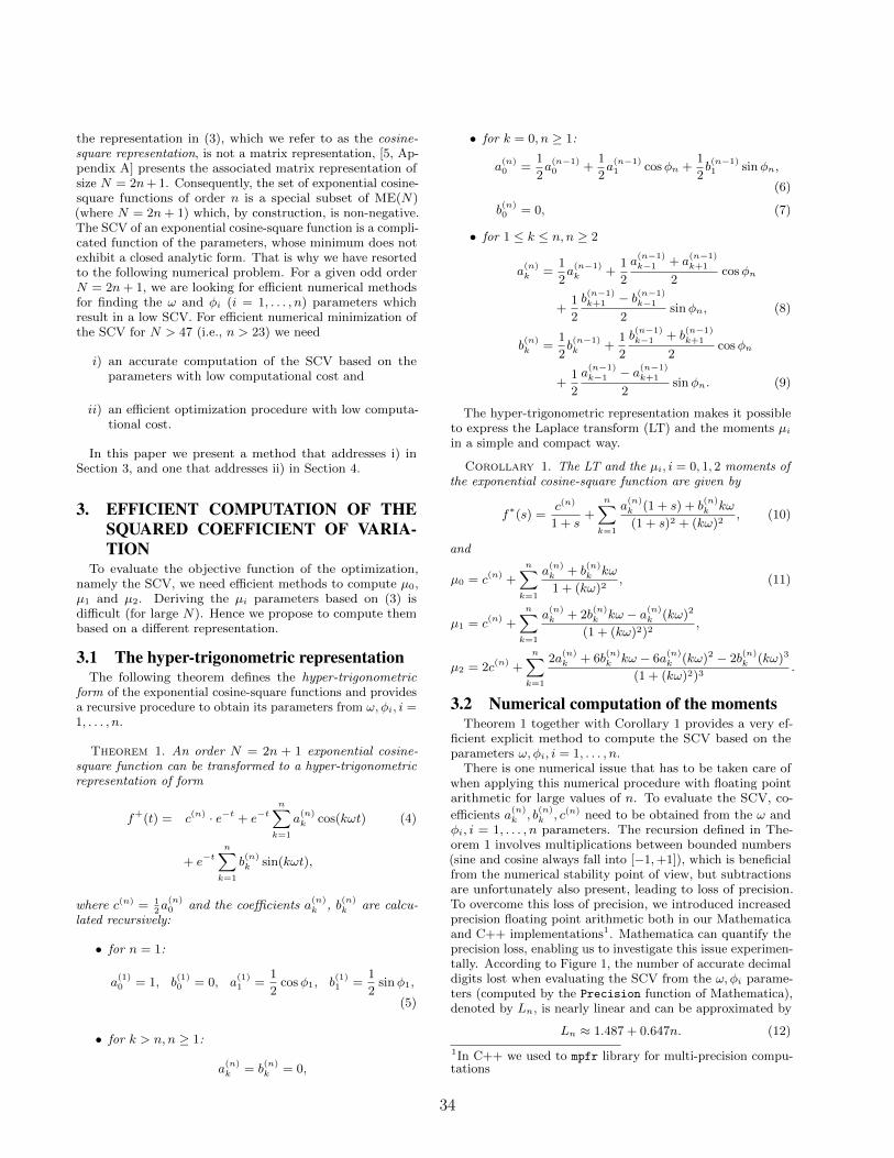
the representation in (3), which we refer to as the cosine-square representation, is not a matrix representation, [5, Ap-pendix A] presents the associated matrix representation ofsize N = 2n+ 1. Consequently, the set of exponential cosine-square functions of order n is a special subset of ME(N)(where N = 2n+ 1) which, by construction, is non-negative.The SCV of an exponential cosine-square function is a compli-cated function of the parameters, whose minimum does notexhibit a closed analytic form. That is why we have resortedto the following numerical problem. For a given odd orderN = 2n+ 1, we are looking for efficient numerical methodsfor finding the ω and φi (i = 1, . . . , n) parameters whichresult in a low SCV. For efficient numerical minimization ofthe SCV for N > 47 (i.e., n > 23) we need

i) an accurate computation of the SCV based on theparameters with low computational cost and

ii) an efficient optimization procedure with low computa-tional cost.

In this paper we present a method that addresses i) inSection 3, and one that addresses ii) in Section 4.

3. EFFICIENT COMPUTATION OF THESQUARED COEFFICIENT OF VARIA-TION

To evaluate the objective function of the optimization,namely the SCV, we need efficient methods to compute µ0,µ1 and µ2. Deriving the µi parameters based on (3) isdifficult (for large N). Hence we propose to compute thembased on a different representation.

3.1 The hyper-trigonometric representationThe following theorem defines the hyper-trigonometric

form of the exponential cosine-square functions and providesa recursive procedure to obtain its parameters from ω, φi, i =1, . . . , n.

Theorem 1. An order N = 2n + 1 exponential cosine-square function can be transformed to a hyper-trigonometricrepresentation of form

f+(t) = c(n) · e−t + e−tn∑

k=1

a(n)k cos(kωt) (4)

+ e−tn∑

k=1

b(n)k sin(kωt),

where c(n) = 12a(n)0 and the coefficients a

(n)k , b

(n)k are calcu-

lated recursively:

• for n = 1:

a(1)0 = 1, b

(1)0 = 0, a

(1)1 =

1

2cosφ1, b

(1)1 =

1

2sinφ1,

(5)

• for k > n, n ≥ 1:

a(n)k = b

(n)k = 0,

• for k = 0, n ≥ 1:

a(n)0 =

1

2a(n−1)0 +

1

2a(n−1)1 cosφn +

1

2b(n−1)1 sinφn,

(6)

b(n)0 = 0, (7)

• for 1 ≤ k ≤ n, n ≥ 2

a(n)k =

1

2a(n−1)k +

1

2

a(n−1)k−1 + a

(n−1)k+1

2cosφn

+1

2

b(n−1)k+1 − b(n−1)

k−1

2sinφn, (8)

b(n)k =

1

2b(n−1)k +

1

2

b(n−1)k−1 + b

(n−1)k+1

2cosφn

+1

2

a(n−1)k−1 − a(n−1)

k+1

2sinφn. (9)

The hyper-trigonometric representation makes it possibleto express the Laplace transform (LT) and the moments µiin a simple and compact way.

Corollary 1. The LT and the µi, i = 0, 1, 2 moments ofthe exponential cosine-square function are given by

f∗(s) =c(n)

1 + s+

n∑

k=1

a(n)k (1 + s) + b

(n)k kω

(1 + s)2 + (kω)2, (10)

and

µ0 = c(n) +n∑

k=1

a(n)k + b

(n)k kω

1 + (kω)2, (11)

µ1 = c(n) +n∑

k=1

a(n)k + 2b

(n)k kω − a(n)k (kω)2

(1 + (kω)2)2,

µ2 = 2c(n) +n∑

k=1

2a(n)k + 6b

(n)k kω − 6a

(n)k (kω)2 − 2b

(n)k (kω)3

(1 + (kω)2)3.

3.2 Numerical computation of the momentsTheorem 1 together with Corollary 1 provides a very ef-

ficient explicit method to compute the SCV based on theparameters ω, φi, i = 1, . . . , n.

There is one numerical issue that has to be taken care ofwhen applying this numerical procedure with floating pointarithmetic for large values of n. To evaluate the SCV, co-

efficients a(n)k , b

(n)k , c(n) need to be obtained from the ω and

φi, i = 1, . . . , n parameters. The recursion defined in The-orem 1 involves multiplications between bounded numbers(sine and cosine always fall into [−1,+1]), which is beneficialfrom the numerical stability point of view, but subtractionsare unfortunately also present, leading to loss of precision.To overcome this loss of precision, we introduced increasedprecision floating point arithmetic both in our Mathematicaand C++ implementations1. Mathematica can quantify theprecision loss, enabling us to investigate this issue experimen-tally. According to Figure 1, the number of accurate decimaldigits lost when evaluating the SCV from the ω, φi parame-ters (computed by the Precision function of Mathematica),denoted by Ln, is nearly linear and can be approximated by

Ln ≈ 1.487 + 0.647n. (12)

1In C++ we used to mpfr library for multi-precision compu-tations

34

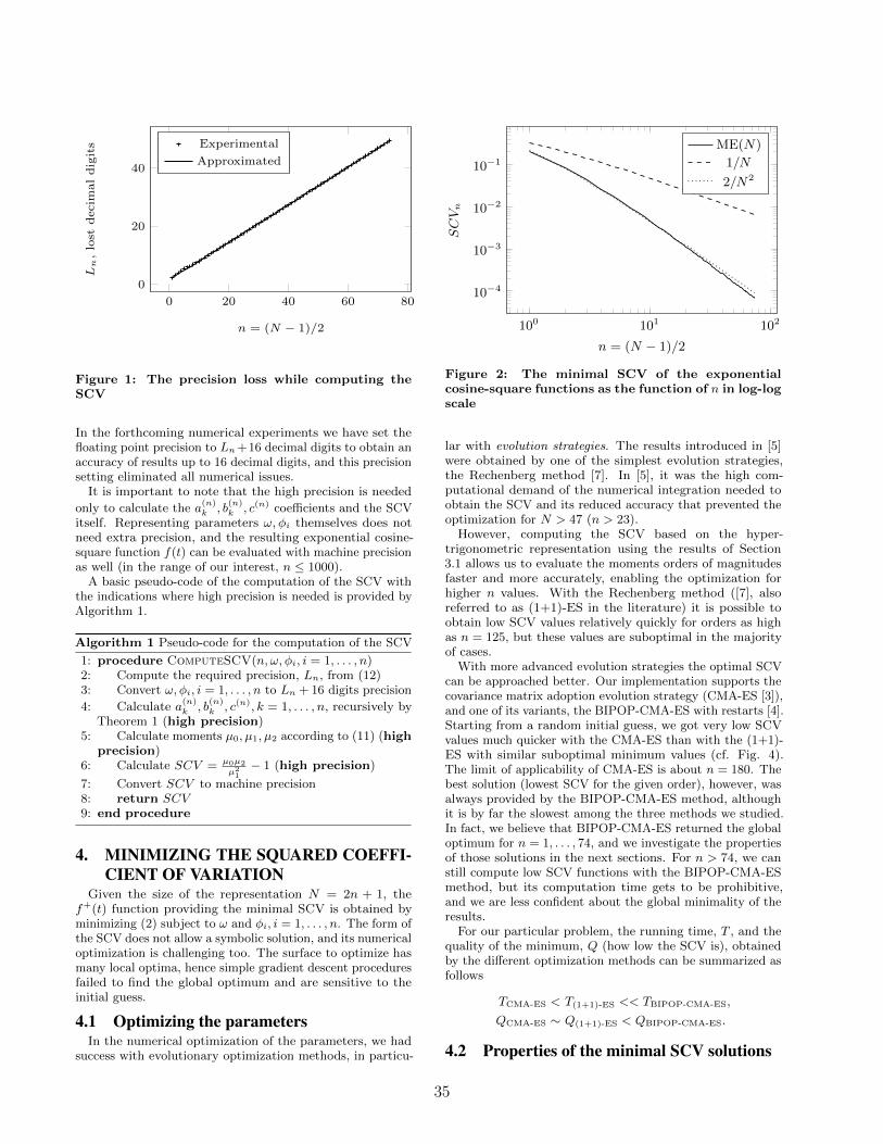
0 20 40 60 80

0

20

40

n = (N − 1)/2

Ln,lost

decim

aldigits Experimental

Approximated

Figure 1: The precision loss while computing theSCV

In the forthcoming numerical experiments we have set thefloating point precision to Ln+16 decimal digits to obtain anaccuracy of results up to 16 decimal digits, and this precisionsetting eliminated all numerical issues.

It is important to note that the high precision is needed

only to calculate the a(n)k , b

(n)k , c(n) coefficients and the SCV

itself. Representing parameters ω, φi themselves does notneed extra precision, and the resulting exponential cosine-square function f(t) can be evaluated with machine precisionas well (in the range of our interest, n ≤ 1000).

A basic pseudo-code of the computation of the SCV withthe indications where high precision is needed is provided byAlgorithm 1.

Algorithm 1 Pseudo-code for the computation of the SCV

1: procedure ComputeSCV(n, ω, φi, i = 1, . . . , n)2: Compute the required precision, Ln, from (12)3: Convert ω, φi, i = 1, . . . , n to Ln + 16 digits precision

4: Calculate a(n)k , b

(n)k , c(n), k = 1, . . . , n, recursively by

Theorem 1 (high precision)5: Calculate moments µ0, µ1, µ2 according to (11) (high

precision)6: Calculate SCV = µ0µ2

µ21− 1 (high precision)

7: Convert SCV to machine precision8: return SCV9: end procedure

4. MINIMIZING THE SQUARED COEFFI-CIENT OF VARIATION

Given the size of the representation N = 2n + 1, thef+(t) function providing the minimal SCV is obtained byminimizing (2) subject to ω and φi, i = 1, . . . , n. The form ofthe SCV does not allow a symbolic solution, and its numericaloptimization is challenging too. The surface to optimize hasmany local optima, hence simple gradient descent proceduresfailed to find the global optimum and are sensitive to theinitial guess.

4.1 Optimizing the parametersIn the numerical optimization of the parameters, we had

success with evolutionary optimization methods, in particu-

100 101 102

10−4

10−3

10−2

10−1

n = (N − 1)/2

SCVn

ME(N)

1/N

2/N2

Figure 2: The minimal SCV of the exponentialcosine-square functions as the function of n in log-logscale

lar with evolution strategies. The results introduced in [5]were obtained by one of the simplest evolution strategies,the Rechenberg method [7]. In [5], it was the high com-putational demand of the numerical integration needed toobtain the SCV and its reduced accuracy that prevented theoptimization for N > 47 (n > 23).

However, computing the SCV based on the hyper-trigonometric representation using the results of Section3.1 allows us to evaluate the moments orders of magnitudesfaster and more accurately, enabling the optimization forhigher n values. With the Rechenberg method ([7], alsoreferred to as (1+1)-ES in the literature) it is possible toobtain low SCV values relatively quickly for orders as highas n = 125, but these values are suboptimal in the majorityof cases.

With more advanced evolution strategies the optimal SCVcan be approached better. Our implementation supports thecovariance matrix adoption evolution strategy (CMA-ES [3]),and one of its variants, the BIPOP-CMA-ES with restarts [4].Starting from a random initial guess, we got very low SCVvalues much quicker with the CMA-ES than with the (1+1)-ES with similar suboptimal minimum values (cf. Fig. 4).The limit of applicability of CMA-ES is about n = 180. Thebest solution (lowest SCV for the given order), however, wasalways provided by the BIPOP-CMA-ES method, althoughit is by far the slowest among the three methods we studied.In fact, we believe that BIPOP-CMA-ES returned the globaloptimum for n = 1, . . . , 74, and we investigate the propertiesof those solutions in the next sections. For n > 74, we canstill compute low SCV functions with the BIPOP-CMA-ESmethod, but its computation time gets to be prohibitive,and we are less confident about the global minimality of theresults.

For our particular problem, the running time, T , and thequality of the minimum, Q (how low the SCV is), obtainedby the different optimization methods can be summarized asfollows

TCMA-ES < T(1+1)-ES << TBIPOP-CMA-ES,

QCMA-ES ∼ Q(1+1)-ES < QBIPOP-CMA-ES.

4.2 Properties of the minimal SCV solutions

35

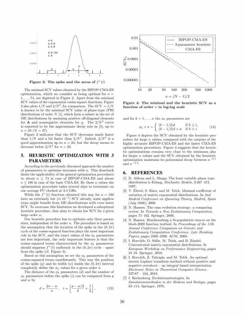
n=6p=4.0w=2.0

d=0.714i=4

wdp

1 2 3 4 5 6

0.0005

0.0010

0.0015

Figure 3: The spike and the zeros of f+(t)

The minimal SCV values obtained by the BIPOP-CMA-ESoptimization, which we consider as being optimal for n =1, . . . , 74, are depicted in Figure 2. Apart from the minimalSCV values of the exponential cosine-square functions, Figure2 also plots 1/N and 2/N2, for comparison. The SCV = 1/Nis known to be the minimal SCV value of phase-type (PH)distributions of order N [1], which form a subset in the set ofME distributions by assuming positive off-diagonal elementsfor A and nonnegative elements for α. The 2/N2 curveis reported to be the approximate decay rate in [5], up ton = 23 (N = 47).

Figure 2 indicates that the SCV decreases much fasterthan 1/N and a bit faster than 2/N2. Indeed, 2/N2 is agood approximation up to n = 23, but the decay seems todecrease below 2/N2 for n > 23.

5. HEURISTIC OPTIMIZATION WITH 3PARAMETERS

According to the previously discussed approach the numberof parameters to optimize increases with n. This drawbacklimits the applicability of the general optimization proceduresto about n ≤ 74 in case of BIPOP-CMA-ES and aboutn ≤ 180 in case of the basic CMA-ES. By these n values theoptimization procedure takes several days to terminate onour average PC clocked at 3.4 GHz.

While the f+(t) function obtained this way for n = 180have an extremely low (≈ 10−5) SCV already, some applica-tions might benefit from ME distributions with even lowerSCV. To overcome this limitation we developed a suboptimalheuristic procedure, that aims to obtain low SCV for a givenlarge order n.

Our heuristic procedure has to optimize only three param-eters, independent of the order n. The procedure is based onthe assumption that the location of the spike in the (0, 2π)cycle of the cosine-squared function plays the most importantrole in the SCV, and the exact values of the φk parametersare less important, the only important feature is that thecosine-squared terms characterized by the φk parametersshould suppress f+(t) uniformly in the (0, 2π) cycle – apartfrom the spike (cf. Figure 3).

Based on this assumption we set the φk parameters of thecosine-squared terms equidistantly. This way the positionof the spike (p) and its width (w) inside the (0, 2π) intervalcompletely define the φk values for a given order n.

The distance of the φk parameters (d) and the number ofφk parameters before the spike (i) can be computed from pand w by

d =2π − wn

, i =

⌊p− w/2

d+

1

2

⌋, (13)

10 20 50 100 200 500 1000

0.000001

0.00001

0.0001

0.001

0.01

n = (N − 1)/2

SCVn

BIPOP-CMA-ES

3-parameter heuristic

CMA-ES

Figure 4: The minimal and the heuristic SCV as afunction of order n in log-log scale

and for k = 1, . . . , n the φk parameters are

φk + π =

(k − 1/2)d if k ≤ i,(k − 1/2)d+ w if k > i.

(14)

Figure 4 depicts the SCV obtained by the heuristic pro-cedure for large n values, compared with the outputs of thehighly accurate BIPOP-CMA-ES and the faster CMA-ESoptimization procedures. Figure 4 suggests that the heuris-tic optimizations remains very close to the minimum alsofor larger n values and the SCV obtained by the heuristicoptimization maintains its polynomial decay between n−2.1

and n−2.2.

6. REFERENCES[1] D. Aldous and L. Shepp. The least variable phase type

distribution is Erlang. Stochastic Models, 3:467–473,1987.

[2] T. Elteto, S. Racz, and M. Telek. Minimal coefficient ofvariation of matrix exponential distributions. In 2ndMadrid Conference on Queueing Theory, Madrid, Spain(July 2006), 2006.

[3] N. Hansen. The cma evolution strategy: a comparingreview. In Towards a New Evolutionary Computation,pages 75–102. Springer, 2006.

[4] N. Hansen. Benchmarking a bi-population cma-es on thebbob-2009 function testbed. In Proceedings of the 11thAnnual Conference Companion on Genetic andEvolutionary Computation Conference: Late BreakingPapers, pages 2389–2396. ACM, 2009.

[5] I. Horvath, O. Safar, M. Telek, and B. Zambo.Concentrated matrix exponential distributions. InEuropean Workshop on Performance Engineering, pages18–31. Springer, 2016.

[6] I. Horvath, Z. Talyigas, and M. Telek. An optimalinverse Laplace transform method without positive andnegative overshoot – an integral based interpretation.Electronic Notes in Theoretical Computer Science,337:87 – 104, 2018.

[7] I. Rechenberg. Evolutionsstrategien. InSimulationsmethoden in der Medizin und Biologie, pages83–114. Springer, 1978.

36

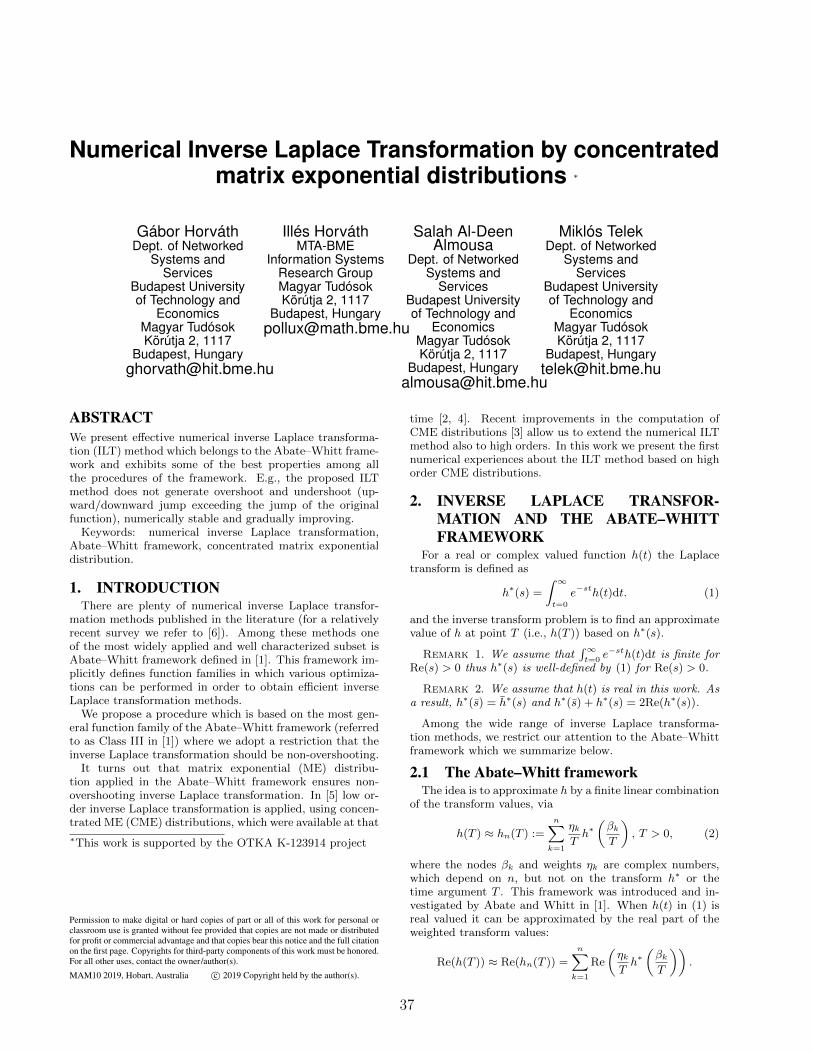
Numerical Inverse Laplace Transformation by concentratedmatrix exponential distributions ∗

Gábor HorváthDept. of Networked

Systems andServices

Budapest Universityof Technology and

EconomicsMagyar TudósokKörútja 2, 1117

Budapest, [email protected]

Illés HorváthMTA-BME

Information SystemsResearch GroupMagyar TudósokKörútja 2, 1117


Salah Al-DeenAlmousa

Dept. of NetworkedSystems and

ServicesBudapest Universityof Technology and



Miklós TelekDept. of Networked

Systems andServices

Budapest Universityof Technology and



ABSTRACTWe present effective numerical inverse Laplace transforma-tion (ILT) method which belongs to the Abate–Whitt frame-work and exhibits some of the best properties among allthe procedures of the framework. E.g., the proposed ILTmethod does not generate overshoot and undershoot (up-ward/downward jump exceeding the jump of the originalfunction), numerically stable and gradually improving.

Keywords: numerical inverse Laplace transformation,Abate–Whitt framework, concentrated matrix exponentialdistribution.

1. INTRODUCTIONThere are plenty of numerical inverse Laplace transfor-

mation methods published in the literature (for a relativelyrecent survey we refer to [6]). Among these methods oneof the most widely applied and well characterized subset isAbate–Whitt framework defined in [1]. This framework im-plicitly defines function families in which various optimiza-tions can be performed in order to obtain efficient inverseLaplace transformation methods.

We propose a procedure which is based on the most gen-eral function family of the Abate–Whitt framework (referredto as Class III in [1]) where we adopt a restriction that theinverse Laplace transformation should be non-overshooting.

It turns out that matrix exponential (ME) distribu-tion applied in the Abate–Whitt framework ensures non-overshooting inverse Laplace transformation. In [5] low or-der inverse Laplace transformation is applied, using concen-trated ME (CME) distributions, which were available at that

∗This work is supported by the OTKA K-123914 project


MAM10 2019, Hobart, Australia c© 2019 Copyright held by the author(s).

time [2, 4]. Recent improvements in the computation ofCME distributions [3] allow us to extend the numerical ILTmethod also to high orders. In this work we present the firstnumerical experiences about the ILT method based on highorder CME distributions.

2. INVERSE LAPLACE TRANSFOR-MATION AND THE ABATE–WHITTFRAMEWORK

For a real or complex valued function h(t) the Laplacetransform is defined as

h∗(s) =

∫ ∞

t=0

e−sth(t)dt. (1)

and the inverse transform problem is to find an approximatevalue of h at point T (i.e., h(T )) based on h∗(s).

Remark 1. We assume that∫∞t=0

e−sth(t)dt is finite forRe(s) > 0 thus h∗(s) is well-defined by (1) for Re(s) > 0.

Remark 2. We assume that h(t) is real in this work. Asa result, h∗(s) = h∗(s) and h∗(s) + h∗(s) = 2Re(h∗(s)).

Among the wide range of inverse Laplace transforma-tion methods, we restrict our attention to the Abate–Whittframework which we summarize below.

2.1 The Abate–Whitt frameworkThe idea is to approximate h by a finite linear combination

of the transform values, via

h(T ) ≈ hn(T ) :=n∑

k=1

ηkTh∗(βkT

), T > 0, (2)

where the nodes βk and weights ηk are complex numbers,which depend on n, but not on the transform h∗ or thetime argument T . This framework was introduced and in-vestigated by Abate and Whitt in [1]. When h(t) in (1) isreal valued it can be approximated by the real part of theweighted transform values:

Re(h(T )) ≈ Re(hn(T )) =n∑

k=1

Re

(ηkTh∗(βkT

)).

37

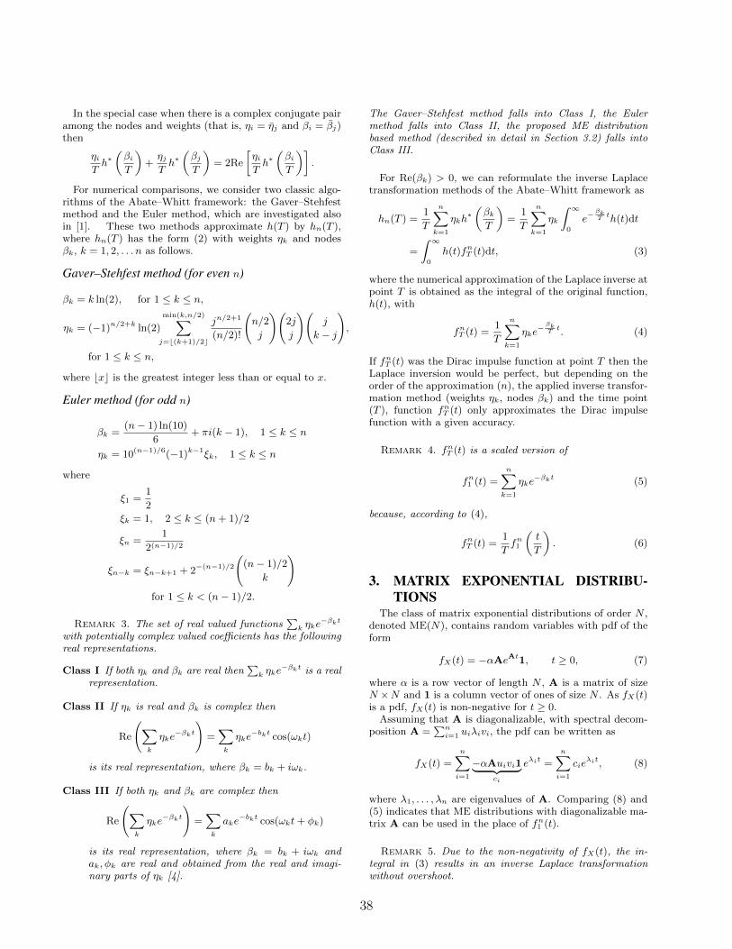
In the special case when there is a complex conjugate pairamong the nodes and weights (that is, ηi = ηj and βi = βj)then

ηiTh∗(βiT

)+ηjTh∗(βjT

)= 2Re

[ηiTh∗(βiT

)].

For numerical comparisons, we consider two classic algo-rithms of the Abate–Whitt framework: the Gaver–Stehfestmethod and the Euler method, which are investigated alsoin [1]. These two methods approximate h(T ) by hn(T ),where hn(T ) has the form (2) with weights ηk and nodesβk, k = 1, 2, . . . n as follows.

Gaver–Stehfest method (for even n)

βk = k ln(2), for 1 ≤ k ≤ n,

ηk = (−1)n/2+k ln(2)

min(k,n/2)∑

j=b(k+1)/2c

jn/2+1

(n/2)!

(n/2

j

)(2j

j

)(j

k − j

),

for 1 ≤ k ≤ n,

where bxc is the greatest integer less than or equal to x.

Euler method (for odd n)

βk =(n− 1) ln(10)

6+ πi(k − 1), 1 ≤ k ≤ n

ηk = 10(n−1)/6(−1)k−1ξk, 1 ≤ k ≤ n

where

ξ1 =1

2

ξk = 1, 2 ≤ k ≤ (n+ 1)/2

ξn =1

2(n−1)/2

ξn−k = ξn−k+1 + 2−(n−1)/2

((n− 1)/2

k

)

for 1 ≤ k < (n− 1)/2.

Remark 3. The set of real valued functions∑k ηke

−βkt

with potentially complex valued coefficients has the followingreal representations.

Class I If both ηk and βk are real then∑k ηke

−βkt is a realrepresentation.

Class II If ηk is real and βk is complex then

Re

(∑

k

ηke−βkt

)=∑

k

ηke−bkt cos(ωkt)

is its real representation, where βk = bk + iωk.

Class III If both ηk and βk are complex then

Re

(∑

k

ηke−βkt

)=∑

k

ake−bkt cos(ωkt+ φk)

is its real representation, where βk = bk + iωk andak, φk are real and obtained from the real and imagi-nary parts of ηk [4].

The Gaver–Stehfest method falls into Class I, the Eulermethod falls into Class II, the proposed ME distributionbased method (described in detail in Section 3.2) falls intoClass III.

For Re(βk) > 0, we can reformulate the inverse Laplacetransformation methods of the Abate–Whitt framework as

hn(T ) =1

T

n∑

k=1

ηkh∗(βkT

)=

1

T

n∑

k=1

ηk

∫ ∞

0

e−βkTth(t)dt

=

∫ ∞

0

h(t)fnT (t)dt, (3)

where the numerical approximation of the Laplace inverse atpoint T is obtained as the integral of the original function,h(t), with

fnT (t) =1

T

n∑

k=1

ηke− βkTt. (4)

If fnT (t) was the Dirac impulse function at point T then theLaplace inversion would be perfect, but depending on theorder of the approximation (n), the applied inverse transfor-mation method (weights ηk, nodes βk) and the time point(T ), function fnT (t) only approximates the Dirac impulsefunction with a given accuracy.

Remark 4. fnT (t) is a scaled version of

fn1 (t) =n∑

k=1

ηke−βkt (5)

because, according to (4),

fnT (t) =1

Tfn1

(t

T

). (6)

3. MATRIX EXPONENTIAL DISTRIBU-TIONS

The class of matrix exponential distributions of order N ,denoted ME(N), contains random variables with pdf of theform

fX(t) = −αAeAt1, t ≥ 0, (7)

where α is a row vector of length N , A is a matrix of sizeN ×N and 1 is a column vector of ones of size N . As fX(t)is a pdf, fX(t) is non-negative for t ≥ 0.

Assuming that A is diagonalizable, with spectral decom-position A =

∑ni=1 uiλivi, the pdf can be written as

fX(t) =n∑

i=1

−αAuivi1︸︷︷︸ci

eλit =

n∑

i=1

cieλit, (8)

where λ1, . . . , λn are eigenvalues of A. Comparing (8) and(5) indicates that ME distributions with diagonalizable ma-trix A can be used in the place of fn1 (t).

Remark 5. Due to the non-negativity of fX(t), the in-tegral in (3) results in an inverse Laplace transformationwithout overshoot.

38

3.1 Concentrated ME distributionsConcentrated ME(N) distributions with low coefficient of

variation has been calculated in [4] up to N = 47 and in [3]for up to N = 2001, using the following form (for odd N):

fME(t) = c e−λt(N−1)/2∏

i=0

cos2(ωt− φi) (9)

with real values of c, λ, ω and φ1, . . . , φ(N−1)/2 obtained fromnumerical optimization.

3.2 ME distribution-based inverse Laplacetransformation

In order to apply the CME distributions for inverseLaplace transformation (9) needs to be rewritten in a formconsistent with (5):

fME(t) = c e−λt(N−1)/2∏

i=0

cos2(ωt− φi) =N∑

i=1

ηie−βit

where n = (N + 1)/2, η1, β1 are real, and the valuesβ2, . . . , βn have positive imaginary parts. For the detailsof this transformation, see the Appendix of [4].

4. NUMERICAL COMPARISON WITHTHE ME BASED METHOD

In order to investigate the properties of the consideredinverse Laplace transformation methods (Euler, Gaver–Stehfest (Gaver in short), Concentrated ME based (CME)),we performed a set of numerical inverse Laplace transfor-mations for the 6 functions of Table 1 using our Matlab im-plementation, where we applied standard double precisionfloating point The arithmetic for CME and 100 digit preci-sion arithmetic with the Matlab Symbolic Math Toolbox forEuler and Gaver. Numerical properties of the 6 test func-tions are rather similar; we demonstrate them using mainlythe test function btc mod 2.

h(t) e−t sin t 1(t > 1)

h∗(s) 11+s

1s2+1

1se−s

h(t) 1(t > 1)e1−t btc btc mod 2

h∗(s) e−s1+s

1s

1es−1

1s

1es+1

Table 1: Set of test functions

Figures 1 and 2 investigate the dependency of the Gaverand the Euler methods on the order. The Gaver methodfails to follow the alternating feature of the original functionfor low order (n = 10). It produces a smooth curve withsome overshoot for medium order (n = 50), and reaches itslimit of numerical stability, despite using 100 digit precision,at n = 64. The Euler method for low order (n = 11) followsthe alternating feature of the original function for longer; itproduces a smooth curve with more dominant overshoot formedium order (n = 51), and reaches its limit of numericalstability, despite using 100 digit precision, at n = 101.

In comparison, the inverse Laplace transformation ob-tained by the CME method is depicted in Figure 3. TheCME method does not produce overshoot at any order. Sim-ilar to the Euler method, the CME method follows the alter-nating feature of the original function for low order (n = 10).It produces a smooth curve for low, medium (n = 50) and

0 1 2 3 4 5 6 7 8 9 10-1

-0.5

0

0.5

1

1.5

2

ExactGaver(n=10)Gaver(n=50)Gaver(n=64)

Figure 1: h(t) = btc mod2 with Gaver method

high (n = 500) orders using double precision arithmetic.The accuracy of the inverse Laplace transformation contin-uously increases with the order.

Figures 4 and 5 compare the methods for h(t) = btc withlow and medium orders, while Figures 6 and 7 comparethe methods for h(t) = btc mod 2 with the same orders.In each case, the benefit of the non-overshooting inverseLaplace transformation is dominant. Especially, the figureswith medium orders indicate the uncertainties coming fromovershooting inverse Laplace transformation using the morealternating Euler method.

The sharpest increase of the Euler and the CME meth-ods are similar for the same orders. Approximating dis-continuity, the Euler method provides a bit sharper in-crease/decrease than the CME method at a given order,but at the cost of significant overshoots before and after thediscontinuity.

5. REFERENCES[1] J. Abate and W. Whitt. A unified framework for

numerically inverting laplace transforms. INFORMSJournal on Computing, 18(4):408–421, Fall 2006.

[2] T. Elteto, S. Racz, and M. Telek. Minimal coefficient ofvariation of matrix exponential distributions. In 2ndMadrid Conference on Queueing Theory, Madrid, Spain(July 2006), 2006.

[3] G. Horvath, I. Horvath, and M. Telek. High order lowvariance matrix-exponential distributions. Submitted toThe Tenth International Conference on Matrix-AnalyticMethods in Stochastic Models (MAM10), 2019.

[4] I. Horvath, O. Safar, M. Telek, and B. Zambo.Concentrated Matrix Exponential Distributions, pages18–31. Springer International Publishing, Cham, 2016.

[5] I. Horvath, Z. Talyigas, and M. Telek. An optimalinverse Laplace transform method without positive andnegative overshoot – an integral based interpretation.Electronic Notes in Theoretical Computer Science,337:87 – 104, 2018.

[6] Q. Wang and H. Zhan. On different numerical inverselaplace methods for solute transport problems.Advances in Water Resources, 75:80 – 92, 2015.

39

0 1 2 3 4 5 6 7 8 9 10-3

-2

-1

0

1

2

3

ExactEuler(n=11)Euler(n=51)Euler(n=101)

Figure 2: h(t) = btc mod 2 with Euler method

0 1 2 3 4 5 6 7 8 9 10-0.2

0

0.2

0.4

0.6

0.8

1

1.2

ExactCME(n=10)CME(n=50)CME(n=500)

Figure 3: h(t) = btc mod 2 with CME method

0 0.5 1 1.5 2 2.5 3 3.5 4 4.5 5-1

0

1

2

3

4

5

ExactGaver(n=18)Euler(n=17)CME(n=17)

Figure 4: h(t) = btc with low orders

0 0.5 1 1.5 2 2.5 3 3.5 4 4.5 5-1

0

1

2

3

4

5


Figure 5: h(t) = btc with medium orders

0 0.5 1 1.5 2 2.5 3 3.5 4 4.5 5-0.4

-0.2

0

0.2

0.4

0.6

0.8

1

1.2


Figure 6: h(t) = btc mod 2 with low orders

0 0.5 1 1.5 2 2.5 3 3.5 4 4.5 5-0.6

-0.4

-0.2

0

0.2

0.4

0.6

0.8

1

1.2

1.4


Figure 7: h(t) = btc mod 2 with medium orders

40

One-sided Markov additive processes: the threefundamental matrices and the scale function

Keynote speaker

Jevgenijs IvanovsAarhus University, Denmark

ABSTRACTTraditional matrix-analytic models can be viewed as Markovadditive processes with level component living on a latticeand some special behaviour at the boundary. The basicassumption that the level process is skip-free in one directionallows for an in-depth analysis of such models. It turns outthat a somewhat similar analysis is possible in the continuous-time non-lattice case when assuming that the level processis jump-free in one direction. Such model corresponds to aLevy process modulated by a Markov chain with additionaljumps at phase switching epochs, where all jumps are of thesame sign.

This tutorial will focus on some basic theory for one-sidedMarkov additive processes highlighting the links to the tra-ditional matrix-analytic models [3]. In particular, we willconsider the three fundamental matrices: the right-, theleft-solution of a certain matrix equation, and the linkingmatrix of expected occupation times at zero. Moreover, wewill construct the so-called scale (matrix-valued) function [4],and discuss some applications of the theory to insurancerisk [1]. If time allows we will also look at the underlyingspectral theory based on the so-called generalized Jordanchains corresponding to analytic matrix functions [2].

Prior knowledge of Levy processes (Levy-Khintchine for-mula) will not be assumed, but will render this tutorial easierto follow.

1. REFERENCES[1] H. Albrecher and J. Ivanovs (2013). A risk model with

an observer in a Markov environment. Risks 1(3), p.148–161.

[2] B. D’Auria, J. Ivanovs, O. Kella, and M. Mandjes(2010). First passage of a Markov additive process andgeneralized Jordan chains. Journal of Applied Probability47(4), p. 1048–1057.

[3] J. Ivanovs, G. Latouche and P.G. Taylor (2018).One-sided Markov additive processes with lattice andnon-lattice increments. In preparation.



[4] J. Ivanovs and Z. Palmowski (2012). Occupation densitiesin solving exit problems for Markov additive processes andtheir reflections. Stochastic Processes and their Applications122(9), p. 3342–3360.

41

Modelling intensive care units using quasi-birth-deathprocesses

Sarah JamesUniversity of Adelaide

North Terrace, Adelaide, 5005South Australia, Australia

[email protected]

Nigel BeanUniversity of Adelaide


[email protected]

Jonathan TukeUniversity of Adelaide


[email protected]

ABSTRACTAn intensive care unit (ICU) is a crucial and limited resourcein a hospital which is affected by uncertainty and variability.ICUs provide high level care to critically ill patients. Thisincludes burns, cardiothoracic, general medicine and surgical,spinal, and trauma cases, as well as patients who require lifesupport. ICUs have the highest nurse to patient ratios in thehospital and often operate close to capacity. Insufficient re-sources in the ICU causes many negative effects both withinthe ICU and in other connected departments [1].

Queueing theory has been used to model the bed occu-pancy in ICUs for the last 20 years, with a particular focuson using M/M/· and M/PH/· queueing models [1]. Thesequeueing models assume that the arrival process (patientarrivals) is a Poisson process, the service times (length ofstay) follow an exponential or Phase-Type distribution, andmost crucially that the arrival process and service times areindependent of each other. These assumptions are ideal forresearchers as many problems become tractable and the anal-ysis of such queueing models is relatively straightforward.However, several studies have revealed that patients may berefused entry into the ICU due to capacity issues [2], andthat there may be some dependence structure between thearrival process and the service times in an ICU [3]. Withoutindependence between the arrival process and service times,all standard queueing models become invalid.

Our research analyses the patient flow of the ICU at theRoyal Adelaide Hospital, Adelaide, South Australia, Aus-tralia. The Royal Adelaide Hospital (RAH) is the largesthospital in Adelaide, South Australia. Prior to November2017, the RAH was located on North Terrace, Adelaide,containing 680 beds and an ICU capacity of 42 beds. Thedataset used in this research was obtained from the ICUat the RAH and contains de-identified information on 7124patients who arrived to the ICU from 1 October 2014 to 30November 2016. This dataset was also used in the analysis



to demonstrate the dependence structure between patientarrivals and patient length of stay [3].

Varney et al. [3] provided an engineering-style method toprovide a reasonable model of bed occupancy in the ICU atthe RAH. In this talk, we aim to provide a more principledapproach to modelling bed occupancy in ICUs using quasi-birth-and-death processes (QBDs). Although PH/PH/·queues are examples of QBDs, they maintain the indepen-dence between the arrival process and the service times. Byallowing the phases of the arrival process and the servicetimes to interact with each other, QBDs provide the flexibil-ity to model a queueing system with dependence betweenthe arrival process and the service times.

However, little research has been conducted in fitting non-specified queueing models to data from queueing systems. Inparticular, no theory has been developed to statistically fitarbitrary QBD models to bed occupancy data. In this talk,we will describe the approaches we have taken to fit suitableQBDs to the RAH ICU data.

1. REFERENCES[1] J. Bai, A. Fugener, J. Schoenfelder, and J. O. Brunner.

Operations research in intensive care unit management:a literature review. Health care management science,21(1):1–24, 2018.

[2] M. A. Metcalfe, A. Sloggett, and K. McPherson.Mortality among appropriately referred patients refusedadmission to intensive-care units. The Lancet,350(9070):7–11, 1997.

[3] J. Varney, N. Bean, and M. Mackay. The self-regulatingnature of occupancy in ICUs: stochastic homoeostasis.Health care management science, pages 1–20, 2018.

42

An Exact Analysis of a Class of Markovian Bitcoin Models

Kayla JavierSchool of Mathematical and Statistical Sciences

Clemson UniversityMartin Hall, Box 340975

Clemson, South Carolina, USA, [email protected]

Brian FralixSchool of Mathematical and Statistical Sciences

Clemson UniversityMartin Hall, Box 340975

Clemson, South Carolina, USA, [email protected]

ABSTRACTRecently, in the work of Gobel et al [2], two continuous-timeMarkov chain models were introduced in order to modelinteractions between a small pool of miners, and a largercollection of miners, within the Bitcoin blockchain. The firstmodel—Model 1—represents the case where the pool behavesin an honest manner, while the second model—Model 2—attempts to model what can happen when the pool behavesdishonestly, and follows a selfish-mining strategy.

Our first result is a new derivation of the stationary distri-bution (up to a normalizing constant) of Model 1, and wefurther build on the results of [2] by showing that the normal-izing constant can be expressed in closed-form. Furthermore,the Laplace transforms of the transition functions are shownto be just as tractable, if we assume that the larger collectionof miners has the same information about the blockchain asthe smaller pool at time zero.

Our next set of results show that the stationary distributionof Model 2—when it exists—can be calculated exactly aswell, without having to truncate the state space. A similarstatement can be made about the Laplace transforms of thetransition functions of Model 2 as well, if we further assumethat the larger collection of miners has the same informationabout the blockchain as the smaller pool at time zero.

The methods we use to study both models, particularlyModel 2, make use of ideas that often appear in the theoryof matrix-analytic methods, except our analysis makes use ofthe recently-developed random-product technique introducedin [1].



1. REFERENCES[1] Buckingham, P., and Fralix, B. (2015) Some new

insights into Kolmogorov’s criterion, with applicationsto hysteretic queues. Markov Processes and RelatedFields 21, 339-368.

[2] Gobel, J., Keeler, H.P., Krzesinski, A.E., and Taylor,P.G. (2016). Bitcoin blockchain dynamics: theselfish-mine strategy in the presence of propagationdelay. Performance Evaluation 104, 23-41.

43

Nearly-completely decomposable Markovmodulated fluid queues

Sarah DendievelGhent University

SMACS Research GroupSint-Pietersnieuwstraat 41

9000 Gent, [email protected]

Guy LatoucheUniversité libre de BruxellesFaculté des sciences, CP212

Boulevard du Triomphe 21050 Bruxelles, [email protected]

Yuanyuan LiuCentral South University

School of Mathematics andStatistics

Changsha, Hunan, 410083,China

[email protected] Tang

Southern University ofScience and Technology

Department of MathematicsShenzhen, Guangdong,

518055, [email protected]

ABSTRACTWe consider a Markov-modulated fluid queue for which theenvironment is nearly-completely decomposable: the set ofphases is partitioned into subsets in such a way that transi-tion rates between different subsets are order of magnitudessmaller than transition rates between phases in the samesubset. Technically, the generator is of the form

Q(ε) = Q∗ + εG, (1)

where ε is a is a small number and Q∗ is a block-diagonalmatrix, so that the phase process is split into separate pro-cesses when ε = 0. The matrix G is such that Q(ε) is anirreducible generator when ε > 0.

Each subset may be thought of as driving its own fluidqueue and the whole process behaves sometimes like one fluidqueue, sometimes like another. This is a model for a systemwith very slowly varying parameters, and we are interestedin analysing the stationary distribution of the whole system.

If each of the isolated fluid queues is positive recurrent,then the whole system is positive recurrent as well, and weshow that its stationary distribution is approximated, forε → 0, by a properly weighted mixture of the stationarydistributions of the isolated fluid queues. A similar resultholds for finite, discret-time Markov chains, as shown inSimon and Ando [5], Courtois [1] and Schweitzer [4] amongothers. In the recent paper Jiang et al. [2], the authorsanalyse the case of a countable state space and give a recentbibliography.

One may imagine that the whole system is positive recur-



rent when ε > 0, while some of the isolated fluid queuesare transient on their own. In that case, the result men-tioned above may not apply, since such transient isolatedfluid queues do not have a stationary distribution. Instead,we show that some of the probability mass disappears fromsight as ε tends to 0. To make the presentation sufficientlysimple, we assume that there are only two subsets of phases,corresponding respectively to a positive recurrent and to atransient isolated fluid queues.

Latouche and Schweitzer [3] bears some similarity withthe fluid queue analysed here. Our present results, however,are more detailed and more general. In particular, we showthat the usual Riccati equation for the matrix Ψ has three(sub)stochastic solutions for ε = 0, only one of which isphysically relevant as a limit for ε → 0.

1. REFERENCES[1] P. Courtois. Decomposability. Queueing and Computer

Systems Applications. Academic Press, New York, 1977.

[2] S. Jiang, Y. Liu, and Y. Tang. A unified perturbationanalysis framework for countable Markov chains. LinearAlgebra and its Applications, 529:413–440, 2017.

[3] G. Latouche and P. J. Schweitzer. A Markov modulated,nearly completely decomposable M/M/1 queue. In W. J.Stewart, editor, Computations with Markov chains,pages 39–48. Springer, 1995.

[4] P. J. Schweitzer. Perturbation series expansions of nearlycompletely-decomposable Markov chains. In O. Boxma,J. Cohen, and H. Tijms, editors, Teletraffic Analysis andComputer Performance Evaluation, pages 319–328,Amsterdam, 1986. Elsevier, North–Holland.

[5] H. A. Simon and A. Ando. Aggregation of variables indynamic systems. Econometrica, 29:111–138, 1961.

44

Eulerian Numbers and an Explicit Formula for a RandomWalk Generating Function

Barbara MargoliusCleveland State University

Cleveland, Ohio 44115-2214, United [email protected]

ABSTRACTConsider a level independent quasi-birth-death process (QBD)[3][1] with time-varying periodic rates, and N phases in eachlevel. The infinitesimal generator for such a system is givenby

Q(t) =

A00(t) A1(t) · ·A−1(t) A0(t) A1(t) ·

·. . .

. . .. . .

where the blocks Ai(t) are N×N matrices whose componentsare periodic functions representing transition rates. Whenthe system is ergodic, there is an asymptotic periodic solutionto the system of differential equations

∂

∂tpn(t) = pn−1(t)A1(t) + pn(t)A0(t) + pn+1(t)A−1(t)

for n > 0 and boundary condition

∂

∂tp0(t) = p0(t)A00(t) + p1(t)A−1(t)

The vectors pn(t) are of length N . The generating functionfor the asymptotic periodic probabilities is given by

Pz(t) =∫ t

t−1

p0(u)(A00(u)−A0(u)− z−1A−1(u)

)Φz(u, t)du

× (I− Φz(t− 1, t))−1

where Φz(s, t) is the generating function for the correspond-ing unbounded process, that is, the random walk process[2].For this generating function, the coefficients on zn are ma-trices. The (i, j)th component of the coefficient on zn is theprobability of a transition from phase i to phase j and up nlevels.

Φz(s, t) solves the differential equation

∂

∂tΦz(s, t) = Φz(s, t)A(z, t)



where

A(z, t) = zA1(t) + A0(t) + z−1A−1(t).

If we were working with a constant rate process, Φz(s, t)

would be the matrix exponential eA(z)(t−s).In general, an explicit formula for Φz(s, t) is not known. In

this paper, we consider several cases where such a formula isavailable and explore the combinatorial interpretation of theresulting expressions. In particular, we study a single-serverpre-emptive priority queue in which the Eulerian numbersappear[4] and a QBD with Erlang arrivals in which roots ofunity play a role[5].

Pre-emptive Priority Queue with Finite BufferIn the case of the pre-emptive priority queue with finitebuffer space for class-2 customers, out state space is given by(X(t), J(t)) where X(t) gives the number of class-1 customersand J(t) gives the number of class-2 customers at time t. As-sociated with this queue-length process, is a two-dimensionalrandom walk where the level, X(t) is unbounded, and thephase, J(t) ranges from zero to K where K is the size of thebuffer. Let λi(t) give the arrival rate of class i-customersand µi(t) give the service rate of class-i customers. Sinceclass-2 customers are served only when there are no class-1customers in the system, µ2(t) is not part of the expressionfor the random walk generating function.

Let ak(s, t) give the probability of k class-2 arrivals duringthe time-interval (s, t], so that

ak(s, t) =

(∫ tsλ2(u)du

)k

k!e−

∫ ts λ2(u)du.

Define the random walk generating function for a particlemoving to the right at rate λ1(t) and to the left at rate µ1(t)as

βz(s, t)

= exp

∫ t

s

λ1(u)du(z − 1) +

∫ t

s

µ1(u)du(z−1 − 1)

=∞∑

n=−∞PrX(t) = n+ k|X(s) = kzn.

45

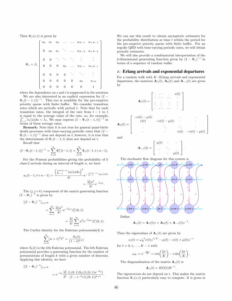
Then Φz(s, t) is given by

Φz = βz

a0 a1 a2 . . . . . . aN−1 a>N−1

0 a0 a1

. . . . . . aN−2 a>N−2

0 0. . .

. . .. . .

......

0 0 0 a0 . . . aN−i a>N−i

0 0 0 0. . .

. . ....

0 0 0 0 0 a0 a>0

0 0 0 0 0 0 1

where the dependence on s and t is suppressed in the notation.We are also interested in an explicit expression for (I −

Φz(t − 1, t))−1. This too is available for the pre-emptivepriority queue with finite buffer. We consider transitionrates which are periodic with period 1. Note that for suchtransition rates, the integral of the rate from t − 1 to tis equal to the average value of the rate, so, for example,∫ tt−1

λ1(u)du = λ1. We may express (I − Φz(t− 1, t))−1 interms of these average rates.

Remark: Note that it is not true for general quasi-birth-death processes with time-varying periodic rates that (I −Φz(t− 1, t))−1 does not depend on t; however, it is true thatthe determinant of Φz(t− 1, t) does not depend on t.

Recall that

(I−Φz(t−1, t))−1 =∞∑

n=0

Φnz (t−1, t) =∞∑

n=0

Φz(t−1, t+n−1).

For the Poisson probabilities giving the probability of kclass-2 arrivals during an interval of length n, we have

ak(t−1, t+n−1) =

(∫ t+n−1

t−1λ2(u)du

)k

k!e−

∫ t+n−1t−1 λ2(u)du

=λk2n

k

k!e−λ2n.

The (j, j+k) component of the matrix generating function(I − Φz)

−1 is given by

[(I − Φz)−1]j,j+k

=∞∑

n=1

λk2nk

k!e−λ2nβnz (0, 1)

=λk2k!

∞∑

n=1

nke−λ2nβnz (0, 1).

The Carlitz identity for the Eulerian polynomials[4] is

∞∑

n=0

(n+ 1)ktn =Sk(t)

(1− t)k+1

where Sk(t) is the kth Eulerian polynomial. The kth Eulerianpolynomial provides a generating function for the number ofpermutations of length k with a given number of descents.Applying this identity, we have

[(I − Φz)−1]j,j+k

= e−λ2λk2k!

βz(0, 1)Sk(βz(0, 1)e−λ2)

(1− e−λ2βz(0, 1))k+1.

We can use this result to obtain asymptotic estimates forthe probability distribution at time t within the period forthe pre-emptive priority queue with finite buffer. For anergodic QBD with time-varying periodic rates, we will obtainperiodic estimates.

We will also provide a combinatorial interpretation of the2-dimensional generating function given by (I − Φz)

−1 interms of a sequence of random walks.

K−Erlang arrivals and exponential departuresFor a random walk with K−Erlang arrivals and exponentialdepartures, the matrices A1(t), A0(t) and A−1(t) are givenby

A1(t) =

· · · · · ν(t)· · · · · · · ·...

......

...· · · · · · · ·

A0(t) =

−ν(t)− µ(t) · · ·ν(t) −ν(t)− µ(t) · ·

·. . .

. . . ·· · ν(t) −ν(t)− µ(t)

and

A−1(t) =

µ(t) · ·

·. . . ·

· · µ(t)

.

The stochastic flow diagram for this system is

j,0

j,1

...

j,K-1

ν

ν

ν

j+1,0

j+1,1

...

j+1,K-1

ν

j-1,0

j-1,1

...

j-1,K-1

µ

µ

µ

ν

µ

µ

µ

ν

ν

ν

ν

ν

ν

j+2,0

j+2,1

...

j+2,K-1

ν

ν

ν

µ

µ

µ

ν

µ

µ

µ

ν

j-2,0

j-2,1

...

j-2,K-1

ν

µ

µ

µ

µ

µ

µ

ν

ν

ν

ν

Define

Az(t) = A1(t)z + A0(t) + A−1(t)z−1.

Then the eigenvalues of Az(t) are given by

ε`(t) = ω−`K ν(t)z1/K − µ(t)− ν(t) + µ(t)z−1

for ` = 0, 1, . . . ,K − 1 with

ωK = e−2πiK = cos

(2π

K

)− i sin

(2π

K

).

The diagonalization of the matrix Az(t) is

Az(t) = HD(t)H−1.

The eigenvectors do not depend on t. This makes the matrixfunction Φz(s, t) particularly easy to compute. It is given in

46

terms of the exponential of the integrals of the diagonals sowe have

Φz(s, t)

= H

e∫ ts ε0(u)du 0 · · · 0

0 e∫ ts ε1(u)du 0

......

. . .. . .

...

0 · · · 0 e∫ ts εK−1(u)du

H−1.

Note that Φz(s, r)Φz(r, t) = Φz(s, t), that is

Φz(s, r)Φz(r, t)

= H

e∫ rs ε0(u)du 0 · · · 0

0 e∫ rs ε1(u)du 0

......

. . .. . .

...

0 · · · 0 e∫ rs εK−1(u)du

×H−1H×

e∫ tr ε0(u)du 0 · · · 0

0 e∫ tr ε1(u)du 0

......

. . .. . .

...

0 · · · 0 e∫ tr εK−1(u)du

H−1

= Φz(s, t)

The normalized eigenvector corresponding to the `th eigen-value, ε`(t) = ω−`K ν(t)z1/K − µ(t)− ν(t) + µ(t)z−1, is

v` =1√K

ω0`K z

K−1K

ω1`K z

K−2K

...

ω(K−2)`K z

1K

ω(K−1)`K z0

.

Define B as a diagonal matrix with diagonal:[zK−1K z

K−2K · · · z0

].

Let H be the matrix whose columns are the normalizedeigenvectors. We can write H in terms of a matrix of rootsof unity and the diagonal matrix B. Let

Ω =

ω0K ω0

K · · · ω0K

ω0K ω1

K · · · ωK−1K

.... . .

. . ....

ω0K ωK−1

K · · · ω(K−1)2

K

,

then

H =1√KBΩ,

and H−1 is then given by

H−1 =1√K

ΩB−1

where Ω is the complex conjugate of the matrix Ω.

For general K, an explicit formula for the (m, j) componentof Φz(s, t) is

[Φz(s, t)]m,j

=zj−mK e

∫ ts (−µ(u)−ν(u)+µ(u)z−1)du

K

K−1∑

`=0

e∫ ts ω

`Kν(u)z1/Kduω

`(j−m)K

= e−∫ ts (ν(u)+µ(u)−µ(u)z−1)du

∞∑

n=1

(∫ tsν(u)du

)Kn−j+m

(Kn− j +m)!zn

The (m, j) component depends on j −m, the distance fromthe diagonal and not on j and m separately. Φz(s, t) is aToeplitz matrix.

The structure of the Φz(t−1, t) matrix makes it particularlysimple to compute the matrix (I − Φz(t− 1, t))−1:

(I − Φz(t− 1, t))−1 = Hdiag

[1

1− eεi

]H−1.

This result readily yields formulas suitable for asymptoticanalysis, that is, asymptotic in the level of the process.

SummaryExplicit formulas are seldom available for the random walkgenerating functions associated with level independent QBDswith time-varying periodic rates. In the special circumstanceswhere they are available, they can be exploited to better un-derstand the combinatorial properties of the process, andto facilitate asymptotic (in the level) analysis of the distri-bution. It is hoped that insights gained from processes forwhich explicit formulas are known may be extended to moregeneral QBDs with time-varying periodic rates.

1. REFERENCES[1] G. Latouche and V. Ramaswami. Introduction to Matrix

Analytic Methods in Stochastic Modelling, 1st edition.Chapter 2: PH Distributions. ASA SIAM, 1999.

[2] B. H. Margolius. The matrices R and G of matrixanalytic methods and the time-inhomogeneous periodicquasi-birth-and-death process. Queueing Systems,60(1-2):131–151, 2008.

[3] M. F. Neuts. Matrix-Geometric Solutions in StochasticModels: an Algorithmic Approach, Chapter 2:Probability Distributions of Phase Type. DoverPublications Inc., 1981.

[4] T. K. Petersen. Eulerian Numbers. Birkhauser, 2015.

[5] L. Takacs. Transient behavior of queueing processes witherlang input. Transactions of the AmericanMathematical Society, 100(1):1–28, 1961.

47

Asymptotic periodic analysis of cyclic stochastic fluidflows with time-varying transition rates

Barbara MargoliusCleveland State University

Cleveland, Ohio 44115-2214, United [email protected]



ABSTRACTConsider a cyclic stochastic fluid model (X(t), J(t)) : t ≥ 0with level variable X(t) ≥ 0 and phase variable J(t) ∈ S,driven by a continuous-time Markov chain J(t) : t ≥ 0with a time-varying generator T (t) = [T (t)ij ]i,j∈S and cycleof length 1 such that T (t) = T (t+ 1) for all t ≥ 0.

Assume real-valued rates cJ(t) ∈ R such that when X(t) >

0 then the level X(t) changes at rate cJ(t), and when X(t) = 0

then the level X(t) changes at rate max0, cJ(t).

Let S0 = i ∈ S : ci = 0, S+ = i ∈ S : ci > 0,S− = i ∈ S : ci < 0, and partition the generator T (t)according to S = S0 ∪ S+ ∪ S−, with

T (t) =

T00(t) T0+(t) T0−(t)T+0(t) T++(t) T+−(t)T−0(t) T−+(t) T−−(t)

.

Consider the asymptotic periodic distribution of the modelcorresponding to the observations at time points t ∈ [0, 1)within the cycle, which consists of density π(t;x), t ∈ [0, 1),x > 0, partitioned according to S = S+ ∪ S− ∪ S0,

π(t;x) =[π(t;x)+ π(t;x)− π(t;x)0

], (1)

such that for all t ∈ [0, 1) and i ∈ S,

π(t;x)i =∂

∂x

∞∑

n=0

P (X(t+ n) ≤ x, J(t+ n) = i), (2)

and mass at zero, also partitioned according to S = S+ ∪S− ∪ S0,

p(t) =[0 p−(t) p0(t)

], (3)

∗We would like to thank the Australian Research Council forfunding this research through Linkage Project LP140100152.†ARC Centre of Excellence for Mathematical and StatisticalFrontiers.



such that for all t ∈ [0, 1) and i ∈ S− ∪ S0,

p(t)i =∞∑

n=0

P (X(t+ n) = 0, J(t+ n) = i). (4)

The aim of this research is to derive theoretical expressionsand algorithms for the asymptotic periodic distribution of themodel. This work is an extension of the results in Margoliusand O’Reilly [1], where the model was introduced.

1. REFERENCES[1] B. H. Margolius and M. M. O’Reilly. The analysis of

cyclic stochastic fluid flows with time-varying transitionrates. Queueing Systems, 82(1-2):43–73, 2016.

48

A new numerical method for computing thequasi-stationary distribution of subcritical Galton-Watson

branching processes

Sophie HautphenneUniversity of MelbourneParkville Victoria 3010Melbourne, Australia

[email protected]

Stefano MasseiÉcole polytechnique fédérale

de LausanneLausanne 1015, [email protected]

ABSTRACTBranching processes [1] describe the dynamics of a popula-tion of individuals which reproduce and die independently,according to some specific probability distributions. Moreprecisely, we assume that any individual has a unit lifetime,at the end of which it might give birth to one or more off-springs simultaneously. This is encoded into the probabilitygenerating function P (z) :=

∑j∈N pjz

j where pj is the prob-ability of generating j individuals. These kind of processesare known in the literature as Galton-Watson processes.

We consider populations that are certain to become extinct,yet appear to be stationary over any reasonable time scale.More precisely, we are interested in characterizing the quasi-stationary distribution of the process, i.e., the asymptoticdistribution of the population size, conditional on its survival.

Yaglom [2] proved that if m := P ′(1) ∈ (0, 1) then thequasi stationary distribution exists and its probability gener-ating function G(z) :=

∑j∈N gjz

j solves the Schroder func-tional equation

G(P (z)) = mG(z) + 1−m, ∀z ∈ [0, 1]. (1)

We study the link between the regularity of P (z) and thatof G(z) and we propose a strategy for solving (1).

In the case where P (z) and G(z) are analytic on a disc ofradius r > 1, we rewrite (1) as

∫

|t|=r

G(t)

t− P (z)dt = mG(z) + 1−m, ∀|z| ≤ r. (2)

The discretization of (2) leads to a numerical method thatis capable to find arbitrary accurate approximations of thecoefficients of G(z). Moreover, we point out the (numerical)low-rank structure that appears in the discretized problem,and we show how to exploit it in the proposed procedure.Numerical tests confirm the nice scalability of the computa-tional cost with respect to the accuracy of the approximationof G(z). Finally, we discuss the extension of the technique



to multi-type processes and how to deal with the curse ofdimensionality.

1. REFERENCES[1] T. E. Harris. The theory of branching processes. Courier

Corporation, 2002.

[2] A. M. Yaglom. Certain limit theorems of the theory ofbranching random processes. In Doklady Akad. NaukSSSR (NS), volume 56, page 3, 1947.

49

Rate of strong convergence of stochastic fluid processesto Markov-modulated Brownian motion

Keynote speaker

Giang NguyenSchool of Mathematical Sciences

The University of AdelaideAdelaide, Australia

[email protected]

Oscar Peralta-GutierrezSchool of Mathematical Sciences

The University of AdelaideAdelaide, Australia

[email protected]

ABSTRACTIn [2], the authors constructed a sequence of stochastic fluidprocesses and showed that it converges weakly to a Markov-modulated Brownian motion (Xt, ϕt)t≥0.

Here, we construct another sequence of stochastic fluidprocesses, with different characteristics to the ones consideredin [2], and show that it converges strongly to (Xt, ϕt)t≥0.We also show that the rate of this almost sure convergenceis proportional to n−1/2 logn.

When reduced to the special case of standard Brownianmotion, our convergence rate is an improvement over thatobtained by [1], which is proportional to n−1/2(logn)5/2.

1. REFERENCES[1] L. G. Gorostiza and R. J. Griego. Rate of convergence of

uniform transport processes to Brownian motion andapplication to stochastic integrals. Stochastics,3(1-4):291–303, 1980.

[2] G. Latouche and G. T. Nguyen. The morphing of fluidqueues into Markov-modulated Brownian motion.Stochastic Systems, 5(1):62–86, 2015.



50

One-sided Markov additive processes: exit problems andrelated topics

Keynote speaker

Zbigniew PalmowskiWrocław University of Science and Technology

ABSTRACTThis tutorial continues the story of Markov additive processespresented by Jevgenijs Ivanovs, focusing on exit problems andpossible applications in applied probability intimately relatedwith queueing theory, risk theory and financial mathematics.

At the beginning, we discuss main ideas presented in [2]and [3] corresponding to exit identities and potential mea-sures. Later, following [4] and [6], we consider the seminalWiener-Hopf factorization. We will also mention new modelsbased on random observations (see [5]) and on the killingthat depends on the state of the Markov additive processes(see [1]).

At the end of the tutorial we show extended list of possibleapplications of the above mentioned theory.

1. REFERENCES[1] I. Czarna, A. Kaszubowski, S. Li and Z. Palmowski

(2018). Fluctuation identities for omega-killed Markovadditive processes and dividend problem. Submitted forpublication, https://arxiv.org/abs/1806.08102.

[2] J. Ivanovs and Z. Palmowski (2012). Occupationdensities in solving exit problems for Markov additiveprocesses and their reflections. Stochastic Processes andtheir Applications 122(9), p. 3342–3360.

[3] J. Ivanovs (2014). Potential measures of one-sidedMarkov additive processes with reflecting andterminating barriers. Journal of Applied Probability51(4), 2014, p. 1154–1170.

[4] J. Ivanovs (2017). Splitting and time reversal for Markovadditive processes. Stochastic Processes and TheirApplications 127(8), p. 2699–2724.

[5] J. Ivanovs and H. Albrecher (2017). Strikingly simpleidentities relating exit problems for Levy processesunder continuous and Poisson observations. StochasticProcesses and Their Applications 127(2), p. 643–656.

[6] P. Klusik and Z. Palmowski (2014). A note onWiener-Hopf factorization for spectrally negative MarkovAdditive processes. Journal of Theoretical Probability 27,



p. 202–219.

51

Quasi stationarity

Keynote speaker

Phil PollettThe University of Queensland

ABSTRACTMany biological systems are predicted to “die out”, yet theypersist over any reasonable time scale. This phenomenon,termed quasi stationarity, is apparent in many biologicalsystems: a population may persist over many years; aninfection may become endemic in a population; a chronicallyill patient may survive for a long period of time. I will reviewseveral approaches to modelling this behaviour.



52

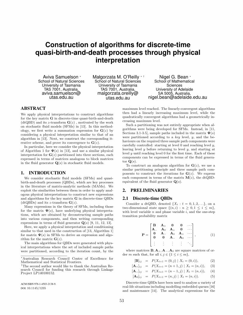
Construction of algorithms for discrete-timequasi-birth-and-death processes through physical

interpretation

Aviva Samuelson ∗

School of Natural SciencesUniversity of TasmaniaTAS 7001, Australia,

[email protected]

Małgorzata M. O’Reilly ∗ †School of Natural Sciences

University of TasmaniaTAS 7001, Australia,

[email protected]

Nigel G. Bean ∗

School of MathematicalSciences

University of AdelaideSA 5005, Australia,

[email protected]

ABSTRACTWe apply physical interpretations to construct algorithmsfor the key matrix G in discrete-time quasi-birth-and-death(dtQBD) and its z-transform G(z) , motivated by the workon stochastic fluid models (SFMs) in [13]. In this method-ology, we first write a summation expression for G(z) byconsidering a physical interpretation similar to that of analgorithm in [13]. Next, we construct the corresponding it-erative scheme, and prove its convergence to G(z).

In particular, here we consider the physical interpretationof Algorithm 1 for Ψ(s) in [13], and use a similar physicalinterpretation for G(z) partitioned into three sections, eachexpressed in terms of matrices analogous to block matricesin the fluid generator Q(s) in stochastic fluid models.

1. INTRODUCTIONWe consider stochastic fluid models (SFMs) and quasi-

birth-and-death processes (QBDs), which are key processesin the literature of matrix-analytic methods (MAMs). Weexploit the similarities between them in order to apply anal-ogous physical interpretations to construct new expressionsand algorithms for the key matrix G in discrete-time QBDs(dtQBDs) and its z-transform G(z).

Many expressions in the theory of SFMs, including thosefor the matrix Ψ(s), have underlying physical interpreta-tions, which are obtained by deconstructing sample pathsinto various components, and then writing correspondingexpressions in terms of fluid generator Q(s) [9, 11, 12, 13].

Here, we apply a physical interpretation and conditioningsimilar to that used in the construction of [13, Algorithm 1]for matrix Ψ(s) in SFMs to derive an expression and algo-rithm for the matrix G(z).

The main algorithms for QBDs were generated with phys-ical interpretations where the set of included sample pathswere partitioned, according to the iteration count, by the

∗Australian Research Council Centre of Excellence forMathematical and Statistical Frontiers.†The second author would like to thank the Australian Re-search Council for funding this research through LinkageProject LP140100152.

ACM ISBN 978-1-4503-2138-9.

DOI: 10.1145/1235

maximum level reached. The linearly-convergent algorithmsthen had a linearly increasing maximum level, while thequadratically convergent algorithms had a geometrically in-creasing maximum level.

Such a partitioning was not entirely appropriate when al-gorithms were being developed for SFMs. Instead, in [11,Sections 3.1-3.5], sample paths included in the matrix Ψ(s)were partitioned according to a key level, y, and the be-haviours on the required three sample path components werecarefully controlled: starting at level 0 and reaching level y,leaving level y before returning to level y, and starting atlevel y until reaching level 0 for the first time. Each of thesecomponents can be expressed in terms of the fluid genera-tor Q(s).

To construct an analogous algorithm for G(z), we use asimilar partitioning principle and three sample path com-ponents to construct the iterations for G(z). We expresseach component in terms of the matrix M(z), the dtQBD-equivalent of the fluid generator Q(s).

2. PRELIMINARIES

2.1 Discrete-time QBDsConsider a dtQBD, denoted Xt : t = 0, 1, 2, . . ., on a

two-dimensional state space (n, i) : n ≥ 0, 1 ≤ i ≤ m,with level variable n and phase variable i, and the one-steptransition probability matrix

P =

B A+ 0 0 · · ·A− A0 A+ 0 · · ·0 A− A0 A+ · · ·0 0 A− A0 · · ·...

......

.... . .

, (1)

where matrices B,A+,A−,A0 are square matrices of or-der m such that, for all i, j ∈ 1 ≤ i ≤ m,

[B]ij = P (Xt+1 = (0, j) | Xt = (0, i)), (2)

[A+]ij = P (Xt+1 = (n+ 1, j) | Xt = (n, i)), (3)

[A−]ij = P (Xt+1 = (n− 1, j) | Xt = (n, i)), (4)

[A0]ij = P (Xt+1 = (n, j) | Xt = (n, i)). (5)

Discrete-time QBDs have been used to analyse a variety ofreal-life situations including modelling embedded queues [16]and maintenance [14]. The analytical expressions for the

53

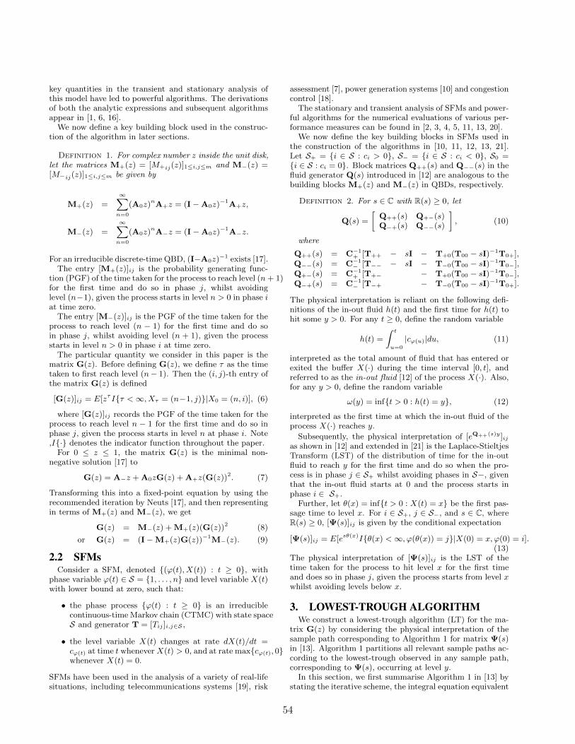
key quantities in the transient and stationary analysis ofthis model have led to powerful algorithms. The derivationsof both the analytic expressions and subsequent algorithmsappear in [1, 6, 16].

We now define a key building block used in the construc-tion of the algorithm in later sections.

Definition 1. For complex number z inside the unit disk,let the matrices M+(z) = [M+ij(z)]1≤i,j≤m and M−(z) =[M−ij(z)]1≤i,j≤m be given by

M+(z) =∞∑

n=0

(A0z)nA+z = (I−A0z)

−1A+z,

M−(z) =∞∑

n=0

(A0z)nA−z = (I−A0z)

−1A−z.

For an irreducible discrete-time QBD, (I−A0z)−1 exists [17].

The entry [M+(z)]ij is the probability generating func-tion (PGF) of the time taken for the process to reach level (n+ 1)for the first time and do so in phase j, whilst avoidinglevel (n−1), given the process starts in level n > 0 in phase iat time zero.

The entry [M−(z)]ij is the PGF of the time taken for theprocess to reach level (n − 1) for the first time and do soin phase j, whilst avoiding level (n + 1), given the processstarts in level n > 0 in phase i at time zero.

The particular quantity we consider in this paper is thematrix G(z). Before defining G(z), we define τ as the timetaken to first reach level (n− 1). Then the (i, j)-th entry ofthe matrix G(z) is defined

[G(z)]ij = E[zτIτ <∞, Xτ = (n−1, j)|X0 = (n, i)], (6)

where [G(z)]ij records the PGF of the time taken for theprocess to reach level n − 1 for the first time and do so inphase j, given the process starts in level n at phase i. Note,I· denotes the indicator function throughout the paper.

For 0 ≤ z ≤ 1, the matrix G(z) is the minimal non-negative solution [17] to

G(z) = A−z + A0zG(z) + A+z(G(z))2. (7)

Transforming this into a fixed-point equation by using therecommended iteration by Neuts [17], and then representingin terms of M+(z) and M−(z), we get

G(z) = M−(z) + M+(z)(G(z))2 (8)

or G(z) = (I−M+(z)G(z))−1M−(z). (9)

2.2 SFMsConsider a SFM, denoted (ϕ(t), X(t)) : t ≥ 0, with

phase variable ϕ(t) ∈ S = 1, . . . , n and level variable X(t)with lower bound at zero, such that:

• the phase process ϕ(t) : t ≥ 0 is an irreduciblecontinuous-time Markov chain (CTMC) with state spaceS and generator T = [Tij ]i,j∈S ,

• the level variable X(t) changes at rate dX(t)/dt =cϕ(t) at time t wheneverX(t) > 0, and at rate maxcϕ(t), 0whenever X(t) = 0.

SFMs have been used in the analysis of a variety of real-lifesituations, including telecommunications systems [19], risk

assessment [7], power generation systems [10] and congestioncontrol [18].

The stationary and transient analysis of SFMs and power-ful algorithms for the numerical evaluations of various per-formance measures can be found in [2, 3, 4, 5, 11, 13, 20].

We now define the key building blocks in SFMs used inthe construction of the algorithms in [10, 11, 12, 13, 21].Let S+ = i ∈ S : ci > 0, S− = i ∈ S : ci < 0, S0 =i ∈ S : ci = 0. Block matrices Q++(s) and Q−−(s) in thefluid generator Q(s) introduced in [12] are analogous to thebuilding blocks M+(z) and M−(z) in QBDs, respectively.

Definition 2. For s ∈ C with R(s) ≥ 0, let

Q(s) =

[Q++(s) Q+−(s)Q−+(s) Q−−(s)

], (10)

where

Q++(s) = C−1+ [T++ − sI − T+0(T00 − sI)−1T0+],

Q−−(s) = C−1− [T−− − sI − T−0(T00 − sI)−1T0−],

Q+−(s) = C−1+ [T+− − T+0(T00 − sI)−1T0−],

Q−+(s) = C−1− [T−+ − T−0(T00 − sI)−1T0+].

The physical interpretation is reliant on the following defi-nitions of the in-out fluid h(t) and the first time for h(t) tohit some y > 0. For any t ≥ 0, define the random variable

h(t) =

∫ t

u=0

|cϕ(u)|du, (11)

interpreted as the total amount of fluid that has entered orexited the buffer X(·) during the time interval [0, t], andreferred to as the in-out fluid [12] of the process X(·). Also,for any y > 0, define the random variable

ω(y) = inft > 0 : h(t) = y, (12)

interpreted as the first time at which the in-out fluid of theprocess X(·) reaches y.

Subsequently, the physical interpretation of [eQ++(s)y]ijas shown in [12] and extended in [21] is the Laplace-StieltjesTransform (LST) of the distribution of time for the in-outfluid to reach y for the first time and do so when the pro-cess is in phase j ∈ S+ whilst avoiding phases in S−, giventhat the in-out fluid starts at 0 and the process starts inphase i ∈ S+.

Further, let θ(x) = inft > 0 : X(t) = x be the first pas-sage time to level x. For i ∈ S+, j ∈ S−, and s ∈ C, whereR(s) ≥ 0, [Ψ(s)]ij is given by the conditional expectation

[Ψ(s)]ij = E[esθ(x)Iθ(x) <∞, ϕ(θ(x)) = j|X(0) = x, ϕ(0) = i].(13)

The physical interpretation of [Ψ(s)]ij is the LST of thetime taken for the process to hit level x for the first timeand does so in phase j, given the process starts from level xwhilst avoiding levels below x.

3. LOWEST-TROUGH ALGORITHMWe construct a lowest-trough algorithm (LT) for the ma-

trix G(z) by considering the physical interpretation of thesample path corresponding to Algorithm 1 for matrix Ψ(s)in [13]. Algorithm 1 partitions all relevant sample paths ac-cording to the lowest-trough observed in any sample path,corresponding to Ψ(s), occurring at level y.

In this section, we first summarise Algorithm 1 in [13] bystating the iterative scheme, the integral equation equivalent

54

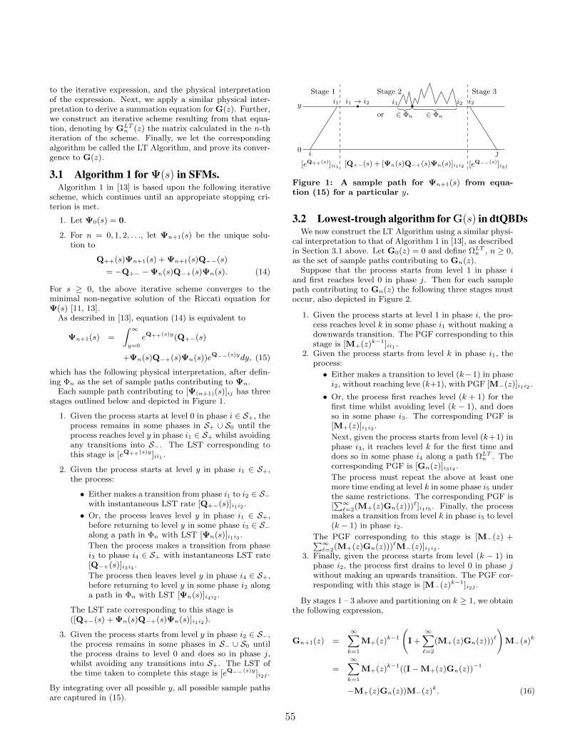
to the iterative expression, and the physical interpretationof the expression. Next, we apply a similar physical inter-pretation to derive a summation equation for G(z). Further,we construct an iterative scheme resulting from that equa-tion, denoting by GLT

n (z) the matrix calculated in the n-thiteration of the scheme. Finally, we let the correspondingalgorithm be called the LT Algorithm, and prove its conver-gence to G(z).

3.1 Algorithm 1 for Ψ(s) in SFMs.Algorithm 1 in [13] is based upon the following iterative

scheme, which continues until an appropriate stopping cri-terion is met.

1. Let Ψ0(s) = 0.

2. For n = 0, 1, 2, . . ., let Ψn+1(s) be the unique solu-tion to

Q++(s)Ψn+1(s) + Ψn+1(s)Q−−(s)

= −Q+− −Ψn(s)Q−+(s)Ψn(s). (14)

For s ≥ 0, the above iterative scheme converges to theminimal non-negative solution of the Riccati equation forΨ(s) [11, 13].

As described in [13], equation (14) is equivalent to

Ψn+1(s) =

∫ ∞

y=0

eQ++(s)y(Q+−(s)

+Ψn(s)Q−+(s)Ψn(s))eQ−−(s)ydy, (15)

which has the following physical interpretation, after defin-ing Φn as the set of sample paths contributing to Ψn.

Each sample path contributing to [Ψ(n+1)(s)]ij has threestages outlined below and depicted in Figure 1.

1. Given the process starts at level 0 in phase i ∈ S+, theprocess remains in some phases in S+ ∪ S0 until theprocess reaches level y in phase i1 ∈ S+ whilst avoidingany transitions into S−. The LST corresponding tothis stage is [eQ++(s)y]ii1 .

2. Given the process starts at level y in phase i1 ∈ S+,the process:

• Either makes a transition from phase i1 to i2 ∈ S−with instantaneous LST rate [Q+−(s)]i1i2 .

• Or, the process leaves level y in phase i1 ∈ S+,before returning to level y in some phase i3 ∈ S−along a path in Φn with LST [Ψn(s)]i1i3 .

Then the process makes a transition from phasei3 to phase i4 ∈ S+ with instantaneous LST rate[Q−+(s)]i3i4 .

The process then leaves level y in phase i4 ∈ S+,before returning to level y in some phase i2 alonga path in Φn with LST [Ψn(s)]i4i2 .

The LST rate corresponding to this stage is([Q+−(s) + Ψn(s)Q−+(s)Ψn(s)]i1i2).

3. Given the process starts from level y in phase i2 ∈ S−,the process remains in some phases in S− ∪ S0 untilthe process drains to level 0 and does so in phase j,whilst avoiding any transitions into S+. The LST ofthe time taken to complete this stage is [eQ−−(s)y]i2j .

By integrating over all possible y, all possible sample pathsare captured in (15).

y

0

Stage 1

i1

i

[eQ++(s)]ii1

Stage 3

i2

j

[eQ−−(s)]i2j

Stage 2

or

[Q+−(s) + [Ψn(s)Q−+(s)Ψn(s)]i1i2

i1 → i2

∈ Φn ∈ Φn

i1 i2

Figure 1: A sample path for Ψn+1(s) from equa-tion (15) for a particular y.

3.2 Lowest-trough algorithm for G(s) in dtQBDsWe now construct the LT Algorithm using a similar physi-

cal interpretation to that of Algorithm 1 in [13], as describedin Section 3.1 above. Let G0(z) = 0 and define ΩLTn , n ≥ 0,as the set of sample paths contributing to Gn(z).

Suppose that the process starts from level 1 in phase iand first reaches level 0 in phase j. Then for each samplepath contributing to Gn(z) the following three stages mustoccur, also depicted in Figure 2.

1. Given the process starts at level 1 in phase i, the pro-cess reaches level k in some phase i1 without making adownwards transition. The PGF corresponding to thisstage is [M+(z)k−1]ii1 .

2. Given the process starts from level k in phase i1, theprocess:

• Either makes a transition to level (k−1) in phasei2, without reaching leve (k+1), with PGF [M−(z)]i1i2 .

• Or, the process first reaches level (k + 1) for thefirst time whilst avoiding level (k − 1), and doesso in some phase i3. The corresponding PGF is[M+(z)]i1i3 .

Next, given the process starts from level (k+1) inphase i3, it reaches level k for the first time anddoes so in some phase i4 along a path ΩLTn . Thecorresponding PGF is [Gn(z)]i3i4 .

The process must repeat the above at least onemore time ending at level k in some phase i5 underthe same restrictions. The corresponding PGF is[∑∞`=2(M+(z)Gn(z)))`]i1i5 . Finally, the process

makes a transition from level k in phase i5 to level(k − 1) in phase i2.

The PGF corresponding to this stage is [M−(z) +∑∞`=2(M+(z)Gn(z)))`M−(z)]i1i2 .

3. Finally, given the process starts from level (k − 1) inphase i2, the process first drains to level 0 in phase jwithout making an upwards transition. The PGF cor-responding with this stage is [M−(z)k−1]i2j .

By stages 1 – 3 above and partitioning on k ≥ 1, we obtainthe following expression,

Gn+1(z) =∞∑

k=1

M+(z)k−1

(I +

∞∑

`=2

(M+(z)Gn(z)))`)

M−(s)k

=∞∑

k=1

M+(z)k−1((I−M+(z)Gn(z))−1

−M+(z)Gn(z))M−(z)k. (16)

55

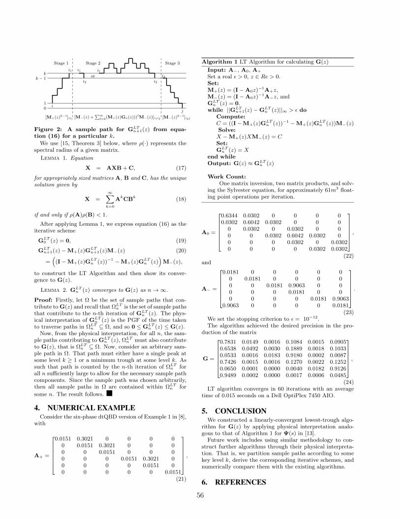
kk − 1

10

Stage 1

i1

i

[M+(z)k−1]ii1

Stage 3

i2

j

[M−(z)k−1]i2j

Stage 2

or

[M−(z) +∑∞`=2(M+(z)Gn(z)))`M−(z)]i1i2

i1

i2

i1

i2

Figure 2: A sample path for GLTn+1(z) from equa-

tion (16) for a particular k.

We use [15, Theorem 3] below, where ρ(·) represents thespectral radius of a given matrix.

Lemma 1. Equation

X = AXB + C, (17)

for appropriately sized matrices A, B and C, has the uniquesolution given by

X =∞∑

k=0

AkCBk (18)

if and only if ρ(A)ρ(B) < 1.

After applying Lemma 1, we express equation (16) as theiterative scheme

GLT0 (z) = 0, (19)

GLTn+1(z)−M+(z)GLT

n+1(z)M−(z) (20)

=(

(I−M+(z)GLTn (z))−1 −M+(z)GLT

n (z))

M−(z),

to construct the LT Algorithm and then show its conver-gence to G(z).

Lemma 2. GLTn (z) converges to G(z) as n→∞.

Proof: Firstly, let Ω be the set of sample paths that con-tribute to G(z) and recall that ΩLTn is the set of sample pathsthat contribute to the n-th iteration of GLT

n (z). The phys-ical interpretation of GLT

n (z) is the PGF of the time takento traverse paths in ΩLTn ⊆ Ω, and so 0 ≤ GLT

n (z) ≤ G(z).Now, from the physical interpretation, for all n, the sam-

ple paths contributing to GLTn (z), ΩLTn must also contribute

to G(z), that is ΩLTn ⊆ Ω. Now, consider an arbitrary sam-ple path in Ω. That path must either have a single peak atsome level k ≥ 1 or a minimum trough at some level k. Assuch that path is counted by the n-th iteration of ΩLTn forall n sufficiently large to allow for the necessary sample pathcomponents. Since the sample path was chosen arbitrarily,then all sample paths in Ω are contained within ΩLTn for

some n. The result follows.

4. NUMERICAL EXAMPLEConsider the six-phase dtQBD version of Example 1 in [8],

with

A+ =

0.0151 0.3021 0 0 0 00 0.0151 0.3021 0 0 00 0 0.0151 0 0 00 0 0 0.0151 0.3021 00 0 0 0 0.0151 00 0 0 0 0 0.0151

,

(21)

Algorithm 1 LT Algorithm for calculating G(z)

Input: A−, A0, A+

Set a real ε > 0, z ∈ Re > 0.Set:M+(z) = (I−A0z)

−1A+z,M−(z) = (I−A0z)

−1A−z, andGLTn (z) = 0.

while ||GLTn+1(z)−GLT

n (z)||∞ > ε doCompute:C = ((I−M+(z)GLT

n (z))−1 −M+(z)GLTn (z))M−(z)

Solve:X −M+(z)XM−(z) = CSet:GLTn (z) = X

end whileOutput: G(z) ≈ GLT

n (z)

Work Count:One matrix inversion, two matrix products, and solv-

ing the Sylvester equation, for approximately 61m3 float-ing point operations per iteration.

A0 =

0.6344 0.0302 0 0 0 00.0302 0.6042 0.0302 0 0 0

0 0.0302 0 0.0302 0 00 0 0.0302 0.6042 0.0302 00 0 0 0.0302 0 0.03020 0 0 0 0.0302 0.0302

,

(22)and

A− =

0.0181 0 0 0 0 00 0.0181 0 0 0 00 0 0.0181 0.9063 0 00 0 0 0.0181 0 00 0 0 0 0.0181 0.9063

0.9063 0 0 0 0 0.0181

.

(23)We set the stopping criterion to ε = 10−12.The algorithm achieved the desired precision in the pro-

duction of the matrix

G =

0.7831 0.0149 0.0016 0.1084 0.0015 0.09050.6538 0.0492 0.0030 0.1889 0.0018 0.10330.0533 0.0016 0.0183 0.9180 0.0002 0.00870.7426 0.0015 0.0016 0.1270 0.0022 0.12520.0650 0.0001 0.0000 0.0040 0.0182 0.91260.9489 0.0002 0.0000 0.0017 0.0006 0.0485

,

(24)LT algorithm converges in 60 iterations with an average

time of 0.015 seconds on a Dell OptiPlex 7450 AIO.

5. CONCLUSIONWe constructed a linearly-convergent lowest-trough algo-

rithm for G(z) by applying physical interpretation analo-gous to that of Algorithm 1 for Ψ(s) in [13].

Future work includes using similar methodology to con-struct further algorithms through their physical interpreta-tion. That is, we partition sample paths according to somekey level k, derive the corresponding iterative schemes, andnumerically compare them with the existing algorithms.

6. REFERENCES

56

[1] S. Ahn, J. Jeon, and V. Ramaswami. Steady stateanalysis of finite fluid flow models using finite qbds.Queueing Systems, 49(3-4):223–259, 2005.

[2] S. Ahn and V. Ramaswami. Fluid flow models andqueues — a connection by stochastic coupling.Stochastic Models, 19(3):325–348, 2003.

[3] S. Ahn and V. Ramaswami. Transient analysis of fluidflow models via stochastic coupling to a queue.Stochastic Models, 20(1):71–101, 2004.

[4] S. Ahn and V. Ramaswami. Efficient algorithms fortransient analysis of stochastic fluid flow models.Journal of Applied Probability, 42(2):531–549, 2005.

[5] S. Asmussen. Stationary distributions for fluid flowmodels with or without Brownian noise. StochasticModels, 11(1):21–49, 1995.

[6] S. Asmussen and M. Pihlsgard. Transient properties ofmany-server queues and related qbds. QueueingSystems, 46(3-4):249–270, 2004.

[7] A. Badescu, L. Breuer, A. da Silva Soares,G. Latouche, M. A. Remiche, and D. Stanford. Riskprocesses analyzed as fluid queues. ScandinavianActuarial Journal, 2005(2):127–141, 2005.

[8] N. Bean, G. Latouche, and P. Taylor. Physicalinterpretations for quasi-birth-and-death processalgorithms. Accepted, 2018.

[9] N. G. Bean and M. M. O’Reilly. Spatially-coherentuniformization of a stochastic fluid model to aquasi-birth-and-death process. PerformanceEvaluation, 70(9):578–592, 2013.

[10] N. G. Bean, M. M. O’Reilly, and J. E. Sargison. Astochastic fluid flow model of the operation andmaintenance of power generation systems. IEEETransactions on Power Systems, 25(3):1361–1374,2010.

[11] N. G. Bean, M. M. O’Reilly, and P. G. Taylor.Algorithms for return probabilities for stochastic fluidflows. Stochastic Models, 21(1):149–184, 2005.

[12] N. G. Bean, M. M. O’Reilly, and P. G. Taylor. Hittingprobabilities and hitting times for stochastic fluidflows. Stochastic processes and their applications,115(9):1530–1556, 2005.

[13] N. G. Bean, M. M. O’Reilly, and P. G. Taylor.Algorithms for the Laplace–Stieltjes transforms of firstreturn times for stochastic fluid flows. Methodologyand Computing in Applied Probability, 10(3):381–408,2008.

[14] B. de Jonge and E. Jakobsons. Optimizing block-basedmaintenance under random machine usage. EuropeanJournal of Operations Research, 265(2):703–709, 2018.

[15] P. Lancaster. Explicit solutions of linear matrixequations. SIAM review, 12(4):544–566, 1970.

[16] G. Latouche and V. Ramaswami. Introduction tomatrix analytic methods in stochastic modeling,volume 5. Society for Industrial Mathematics, 1999.

[17] M. F. Neuts. Matrix-geometric solutions in stochasticmodels: an algorithmic approach. Dover Publications,1981.

[18] M. M. O’Reilly. Multi-stage stochastic fluid models forcongestion control. European Journal of OperationsResearch, 238:514–526, 2014.

[19] M. M. O’Reilly and Z. Palmowski. Loss rates for

stochastic fluid models. Performance Evaluation,70(9):593–606, 2013.

[20] V. Ramaswami. Matrix analytic methods forstochastic fluid flows. In ITC16: InternationalTeletraffic Congress, pages 1019–1030, 1999.

[21] A. Samuelson, M. M. O’Reilly, and N. G. Bean. Onthe generalised reward generator for stochastic fluidmodels: New riccati equation for Ψ. StochasticModels, 33:495–523, 2017.

57

Substitution matrices recapitulate amino acid specificity ofaaRS phylogenies

Julia ShoreUniversity of Tasmania

Churchill AvenueSandy Bay, Tasmania

[email protected]

Barbara HollandUniversity of Tasmania

Churchill AvenueSandy Bay, Tasmania

[email protected] Sumner

University of TasmaniaChurchill Avenue

Sandy Bay, [email protected]

Kay NieseltUniversitat Tubingen

Geschwister-Scholl-PlatzTubingen, Germanykay.nieselt@uni-

tuebingen.de

Peter WillsUniversity of Auckland

Auckland 1010New Zealand

[email protected]

ABSTRACTAminoacyl-tRNA synthase (aaRS) are a set of 20 enzymesessential in the biological process of gene expression. For mostlife forms, they can be divided by their chemical propertiesinto two categories: Class I and Class II [3, 4, 1]. Ouranalysis aimed to find ways of testing the hypothesis thataaRS enzymes came into existence at the same time as thegenetic code and had a role in how it was determined.

The methods for this analysis brought about ways of build-ing a family of stochastic rate matrices from a phylogenetictree which was then fit to empirical data [2]. It was foundthat for a given tree, the set of Markov matrices that couldbe generated formed a closed set under matrix multiplicationand addition.

The results of the analysis found that trees which took intoaccount aaRS class fit data better than randomly generatedtrees. Other chemical properties of interest, particularlypolarity of amino acids, were used to build trees and it wasfound that some types of tree generally fit the data betterthan ones that only took aaRS class into account. However,it was found in these cases that also including aaRS classinto the analysis improved the trees even more.

For further analysis, an F-test was developed to comparethe matrices generated by two nested trees to see if the fitimprovement of their respective matrices was statisticallysignificant. This analysis resulted in confirming that aaRSclass did add significant improvement to trees that took intoaccount other chemical properties.

1. REFERENCES[1] G. Caetano-Anolles, M. Wang, and D. Caetano-Anolles.



Structural phylogenomics retrodicts the origin of thegenetic code and uncovers the evolutionary impact ofprotein flexibility. PLoS One, 8(8):e72225, 2013.

[2] S. Q. Le and O. Gascuel. An improved general aminoacid replacement matrix. Molecular biology andevolution, 25(7):1307–1320, 2008.

[3] P. O’Donoghue and Z. Luthey-Schulten. On theevolution of structure in aminoacyl-trna synthetases.Microbiology and Molecular Biology Reviews,67(4):550–573, 2003.

[4] Y. I. Wolf and E. V. Koonin. On the origin of thetranslation system and the genetic code in the rna worldby means of natural selection, exaptation, andsubfunctionalization. Biology Direct, 2(1):14, 2007.

58

SIR epidemics with stochastic infectious periods

Matthieu SimonUniversity of Melbourne

School of Mathematics and StatisticsVictoria 3010, Australia

[email protected]

ABSTRACTSIR epidemic models describe the spread of an infectious dis-ease in a closed homogeneously mixing population subdividedinto three classes: the susceptibles, the infected individualsand the removed cases. The class of susceptibles containsthe healthy individuals who can become infected. Whencontaminated, a susceptible is contagious for a random dura-tion, called the infectious period. During this period, he cantransmit the disease to the susceptibles, independently ofthe other infected individuals. Then he becomes a removedcase and plays no further role in the spread of the epidemic.

In this work, we consider the case of an SIR epidemic inwhich the infectious periods are represented by an arbitraryabsorbing Markov process. When an individual gets infected,a version of this process starts to govern his period: the rateat which the individual makes contaminations is a function ofthe state occupied by his infection process, and the removaloccurs as soon as it is absorbed.

We use a martingale approach to determine the exactfinal epidemic outcome, that is, the state of the populationwhen there are no more infected individuals. We derivethe distribution of two statistics: the ultimate number ofsusceptibles and the final severity, a measure of the totalcumulative cost due to all infected individuals that emergedduring the course of the epidemic.

Next, we consider a particular case where the infection pro-cesses are represented by Markov-modulated fluid flows, thecontamination rate and severity functions depending on boththe level and the phase. This provides a flexible and tractableclass of models that allow to incorporate different features inthe description of the disease. The continuous variations inthe infection mechanism may reflect, for instance, the periodswhen an individual undergoes a treatment and those when hisillness is worsening. We use techniques from matrix-analyticmethods to refine the results in this setting. We also providea closed expression for the basic reproduction number, oneof the most widely used estimators of the virulence of theepidemic.



59

Models for the evolution of gene-duplicates: Applicationsof Phase-Type distributions


[email protected]



[email protected]

Barbara Holland ∗


[email protected]

David A. Liberles ∗Temple University1900 N 12th StreetPhiladelphia, USA

[email protected]

ABSTRACTGenomes typically contain thousands of genes that performdifferent functions. Rather than all arising independently,these genes group into families that share a common evo-lutionary origin. Gene families arise because of gene dupli-cation, which is thought to be one of the major sources ofevolutionary novelty [4, 6]. However, genes are only pre-served in genomes if they have a function that is maintainedby selection, and at the time of origin a duplicated gene isidentical to another gene with the same functions. A dupli-cate gene can suffer one of several fates [1, 2]: it may be lost(nonfunctionalisation) - effectively destroyed by mutation -leaving its partner to carry out all the gene’s functions; bothcopies may be retained but with complementary and reducedfunctionality (subfunctionalisation); or it may acquire a newfunction (neofunctionalisation) that comes to be protectedby selection.

In 2017 Stark et. al [5] developed and analyzed a math-ematical model for the fate of a pair of duplicated genes.In this model it is assumed that each gene can carry out anumber of functions that are controlled by different regula-tory regions (e.g. different transcription factor binding sitesmight activate the gene in different pathways). All the func-tions are assumed to be protected by selection. Immediatelyfollowing duplication the genes are both able to performall of the functions. Over time mutations (modelled as aPoisson process) are able to knock-out regulatory regions

∗We would like to thank the Australian Research Coun-cil for funding this research through Discovery ProjectDP180100352.†ARC Centre of Excellence for Mathematical and StatisticalFrontiers.



or the coding region of different genes. A mutation to thecoding region of a gene will inactivate all of it’s functions.Eventually the genes will meet one of two fates: either onegene will be lost (nonfunctionalisation) or both genes will beretained but with complementary functions (subfunctionali-sation). The innovation in Stark et. al (2017) was to expressthis stochastic process as an absorbing state Markov chainand to recognize that the results from the rich literature ofPhase-Type distributions [3] could be applied to give analyticsolutions for the time to absorption into different states.

In this talk we will introduce the model above and alsodiscuss some initial results that extend the framework intro-duced in [5] to cases where:

• There are n > 2 gene duplicates.

• New functions can arise due to mutation in an existingregulatory region.

• New functions can arise due to de novo creation of aregulatory region.

1. REFERENCES[1] A. Force, M. Lynch, F. B. Pickett, A. Amores, Y.-l. Yan,

and J. Postlethwait. Preservation of duplicate genes bycomplementary, degenerative mutations. Genetics,151(4):1531–1545, 1999.

[2] M. W. Hahn. Distinguishing among evolutionary modelsfor the maintenance of gene duplicates. Journal ofHeredity, 100(5):605–617, 2009.

[3] G. Latouche and V. Ramaswami. Introduction to matrixanalytic methods in stochastic modeling, volume 5. Siam,1999.

[4] S. Ohno. Evolution by gene duplication springer. NewYork, 1970.

[5] T. L. Stark, D. A. Liberles, B. R. Holland, and M. M.O’Reilly. Analysis of a mechanistic markov model forgene duplicates evolving under subfunctionalization.BMC evolutionary biology, 17(1):38, 2017.

[6] J. S. Taylor and J. Raes. Duplication and divergence:the evolution of new genes and old ideas. Annu. Rev.Genet., 38:615–643, 2004.

60

Models for the evolution of microsatellites


[email protected]



[email protected]

Barbara Holland ∗


[email protected]

ABSTRACTA microsatellite, or simple sequence repeat, is a strand ofDNA which repeats a motif of length 1–6 nucleotides [1]. Forexample, we may have the string of nucleotides ATATATATAT,which is the motif AT repeated 5 times. Microsatellites un-dergo a mutation process, slipped-strand mispairing, whichleads to a change in the number of repeats, at a rate whichis orders of magnitude higher than the rate for other formsof mutation. Most existing microsatellite models focus ontreating slipped-strand mispairing alone, however, it has beenobserved [2, 3, 4] that mutation rate varies between inter-rupted and uninterrupted repeat sequences. This leads to aninteraction effect between point mutations (which introduceinterruptions) and slipped-strand mispairing. The aim of thisproject is to develop new models for microsatellite evolutionwhich treat slipped-strand mispairing together with pointmutation in a biologically realistic manner, and to fit thesemodels to data in order to better understand the dynamicsof microsatellite evolution.

The first part of the project is theoretical. We introducean absorbing level-dependent quasi-birth and death processto model the evolution of microsatellite sequences, with thelevels tracking the conventionally-modelled repeat number,and the phases tracking the extent of interruption in therepeat sequence. This model is developed at the level ofindividual microsatellite sequences, and is then extended toa population-level model by the introduction of a Poissonprocess to model the birth of microsatellites. We then derive atransient distribution for the population-level process, whichcan be fit to some empirical data to estimate, in particular,the extent of the slowdown conferred by interruptions inthe repeat sequence, among other biologically meaningfulparameters.

∗We would like to thank the Australian Research Coun-cil for funding this research through Discovery ProjectDP180100352.†ARC Centre of Excellence for Mathematical and StatisticalFrontiers.



1. REFERENCES[1] H. Ellegren. Microsatellite mutations in the germline:

implications for evolutionary inference. Trends inGenetics, 16(12):551–558, 2000.

[2] A. Estoup, C. Tailliez, J. Cornuet, and M. Solignac. Sizehomoplasy and mutational processes of interruptedmicrosatellites in two bee species, Apis mellifera andBombus terrestris (Apidae). Molecular Biology andEvolution, 12(6):1074–1084, 1995.

[3] P. Jarne and P. Lagoda. Microsatellites, from moleculesto populations and back. Trends in Ecology & Evolution,11(10):424–429, 1996.

[4] L. Wissler, L. Godmann, and E. Bornberg-Bauer.Evolutionary dynamics of simple sequence repeats acrosslong evolutionary time scale in genus Drosophila. Trendsin Evolutionary Biology, 4(1):e7, 2012.

61

The Markov embedding problem: a new look from analgebraic perspective

Michael Baake∗Bielefeld UniversityBielefeld, Germany

[email protected]

Jeremy Sumner†University of Tasmania

Hobart, [email protected]

ABSTRACTRecall that a Markov matrix is said to be “embeddable”if it is expressible as a matrix exponential eQt where Qis a Markov generator. In general this is known to be ahard characterisation problem: Davies [2] provides a usefulsummary of what is known in general, with a complete resultknown only in the 2 × 2 case [3].

Our particular perspective is to address the problem in amodel-specific fashion where we restrict to classes of Markovmatrices satisfying particular algebraic conditions (for exam-ple, symmetric transition probabilities). In this way, we showthat significant progress can be made for particular modelsand our key observation is that there is, in almost all cases,a clear algebraic relation between an embeddable Markovmatrix and its generator. Namely, the generator must belongto the centralizer of the Markov matrix (and vice versa).

To illustrate, we will present the complete solution to the(model-specific) embedding problem for so-called equal-inputmodels. This is an important foundational model class in thecontext of phylogenetic and molecular substitution models.We will also explain the role that complex eigenvalues play inproducing exceptional examples. This is work in preparation[1].

1. REFERENCES[1] M. Baake and J. Sumner. The Markov embedding

problem: a new look from an algebraic perspective. Inpreparation, 2018.

[2] E. B. Davies. Embeddable Markov Matrices. Electron. J.Probab., 15:1474–1486, 2010.

[3] J. F. C. Kingman. The imbedding problem for finitemarkov chains. Zeitschrift fur Wahrscheinlichkeitstheorieund verwandte Gebiete, 1(1):14–24, 1962.

∗Research supported by German Research Foundation(DFG), within the SPP 1590†Research supported by Australian Research ProjectDP180102215



62

Algebraic constraints on the transition probabilitymatrices produced from Lie-Markov models

Jeremy Sumner∗

University of TasmaniaHobart, Tasmania

[email protected]

Julia Shore†

University of TasmaniaHobart, Tasmania

[email protected]

ABSTRACTOver the last 5 years+ our research group has explored aclass of continuous-time Markov chains we like to refer to as“Lie-Markov models” [3]. Each model in this class has thepleasing property of producing substitution matrices thatare closed under matrix multiplication. To date, our pri-mary motivation and focus has been on applications to phy-logenetics and model of molecular substitution. However thegeneral concept of multiplicative closure of a Markov modelushers in a multitude of only partially resolved mathemati-cal questions.

In particular, there is a close relationship to these modelsand the well-known algebraic construction of Lie groups andLie algebras. In that field, the central dogma states that agiven Lie group, which is generally a non-linear set, is moreeasily analysed by passing to its associated Lie algebra (its,linear, tangent space). The Lie group is then recoverable byapplying the exponential map to the Lie algebra (technically,the connected component to the identity is recovered in thisway).

In the context of the Lie-Markov models, the situation isreversed. A Lie-Markov model is defined by choosing a setof generator matrices that form a Lie algebra. The tran-sition probability matrices are then obtained by applyingthe exponential map (as it standard in Markov chain the-ory). However, this construction leaves open the questionof what is the algebraic connection between the structureof the resulting transition probability matrices and the lin-ear constraints that define the Lie algebra of generator ratematrices. A notable result follows: the constraints on thetransition probabilities are non-linear if and only if the gen-erator matrices span a linear subspace that is closed undercommutators (as is required for a Lie algebra) but is notclosed under matrix multiplication.

∗Research supported by Australian Research ProjectDP150100088†Research supported by Australian Research Council Re-search Training Program scholarship


MAM10 2019, Hobart, Australia c⃝ 2019 Copyright held by the owner/author(s).

Somewhat surprisingly, with notable exceptions (e.g. [1]),only a few previous authors have constructive solutions tothis problem in the context of general Lie group theory.

In this talk, we will explain the relevance of the requiredalgebraic structures, explore various illuminating examples,and present an algorithmic approach to finding a solutionfor general Lie-Markov models.

This is work in preparation [2].

1. REFERENCES[1] W. A. de Graaf. Computation with linear algebraic

groups. Chapman and Hall/CRC, 2017.

[2] J. Shore and J. Sumner. Finding the Lie groupassociated to a Lie algebra of matrices. In preparation.

[3] J. G. Sumner, J. Fernandez-Sanchez, and P. D. Jarvis.Lie markov models. Journal of Theoretical Biology,298:16–31, 2012.

63

Maximum likelihood rearrangement distance for circulargenomes

Venta Terauds ∗


[email protected]

Jeremy Sumner ∗


[email protected]

ABSTRACTPhylogenetic modelling attempts to recover the evolutionaryrelationships between present-day biological organisms. Typ-ical input to phylogenetic methods is genomic data such asDNA or amino acid sequences. There are many techniquesavailable, but the predominant modern approach is to modelsequence evolution (be it DNA, amino acids, or other) as acontinuous-time Markov chain on a finite state space andthen use likelihood (or a Bayesian approach) to estimatemodel parameters and the most likely evolutionary history.

In contrast to the point mutation focus of much phylo-genetic modelling, genome rearrangement models comparegenomes with identifiably similar content, such as genes orother large scale genomic units, and focus on differences instructure, such as the order that these units appear in thegenome. Under these models, evolution occurs via rearrange-ment of the genomic units.

The calculation of evolutionary distance via models ofgenome rearrangement has an inherent combinatorial com-plexity. Various algorithms and estimators have been usedto address this, however many of these set quite specificconditions for the underlying model.

We discuss a technique, first presented in in [1] and [2],which applies representation theory to calculate evolutionarydistance between circular genomes as a maximum likelihoodestimate (MLE) of time elapsed. In [3], the implementationof the technique was explored and it was shown that it maybe applied to models with any choice of rearrangements andrelative probabilities thereof. We give the results of someinitial MLE calculations for various models, and show thatone may predict the existence or otherwise of an MLE, fora given pair of genomes, without needing to calculate theentire likelihood function.

∗This work was supported by Australian Research CouncilDiscovery Early Career Research Award DE130100423 toJS and by use of the Nectar Research Cloud, a collabora-tive Australian research platform supported by the NationalCollaborative Research Infrastructure Strategy.



1. REFERENCES[1] S. Serdoz, A. Egri-Nagy, J. Sumner, B. R. Holland, P. D.

Jarvis, M. M. Tanaka, and A. R. Francis. Maximumlikelihood estimates of pairwise rearrangement distances.J. Theoret. Biol., 423:31–40, 2017.

[2] J. G. Sumner, P. D. Jarvis, and A. R. Francis. Arepresentation-theoretic approach to the calculation ofevolutionary distance in bacteria. J. Phys. A,50(33):335601, 14, 2017.

[3] V. Terauds and J. G. Sumner. Maximum likelihoodestimates of rearrangement distance: Implementing arepresentation-theoretic approach. Bull Math Biol, 2018.

64

Polyp fiction: A stochastic fluid model for the AdaptiveBleaching Hypothesis

Max WurmSchool of Mathematical Sciences

The University of AdelaideSA 5005, Australia

[email protected]

Andrew BairdJames Cook UniversityTownsville, Australia

[email protected]

Nigel BeanSchool of Mathematical Sciences


[email protected]

Sean ConnollyJames Cook UniversityTownsville, Australia

[email protected]

Ariella HelfgottEnvironmental Change Institute

Oxford UniversityOX1 2JD, UK

[email protected]

Giang NguyenSchool of Mathematical Sciences


[email protected]

ABSTRACTCoral reefs have a wide variety of functions in ocean ecosys-tems. The process of coral bleaching is a sign of distress, inwhich the coral polyps eject their algal resident. However,some believe that bleaching could be an adaptive responsedesigned to aid in coral’s resilience. This interpretation isknown as the Adaptive Bleaching Hypothesis (ABH). Coral-algal symbiosis is crucial to the survival of reef corals, andthe ABH posits that bleaching encourages changes in thesesymbioses and thus may allow coral to be better adaptedto the stressful environment, should they subsequently bere-colonised by a more suitable clade of algae.

We consider a stochastic fluid model for the ABH, inspiredby the work of Helfgott et al. [1], to model the algal densityin an abstracted coral ‘unit’. We consider the phase processas representing the dominant clade of algae residing in thecoral and the level process to represent the algal density,which is a proxy for the rate of production of energy for thecoral.

The phase process can change organically due to better-adapted clades growing faster and becoming dominant, or bybleaching, after which other clades may or may not colonisethe vacant space. The level input/output rates correspondto algal growth (increasing density), algal decay (decreasingdensity) and bleaching (rapidly decreasing density).

Our primary aim is to model coral mortality throughbleaching, and so we propose that under an algal densitythreshold z, our coral ‘unit’ is not receiving enough energyto sustain itself. We derive the Laplace-Stietljes transformsof times spent below this density threshold, and times toreach the threshold. Thus, we can approximate the timeuntil mortality in our coral ‘unit’ by the time taken for thecoral to reach this threshold as a result of bleaching, and



subsequently exhaust its energy supplies by spending toolong below the threshold.

1. REFERENCES[1] A. Helfgott, N. Bean, S. Connolly, and A. Baird. A

stochastic fluid model of the adaptive bleachinghypothesis on the Great Barrier Reef. Unpublished,2009.

65

9 780646 997070

ISBN 978-0-646-99707-0

· this book forms the proceedings of mam10, and contains 34 abstracts, including 7 extended...

Documents