thesis robert heij final digital version
TRANSCRIPT

7/23/2019 Thesis Robert Heij Final Digital Version
http://slidepdf.com/reader/full/thesis-robert-heij-final-digital-version 1/94
Opportunities for peak shaving electricity
consumption at container terminals
Applying new rules of operation to achieve a more balanced electricity consumption
ROBERT HEIJ
FEBRUARY 2015

7/23/2019 Thesis Robert Heij Final Digital Version
http://slidepdf.com/reader/full/thesis-robert-heij-final-digital-version 2/94
2
Opportunities for peak shaving electricity
consumption at container terminals Applying new rules of operation to achieve a more balanced electricity consumption
Delft University of Technology
Faculty of Technology, Policy and Management
Master program Systems Engineering, Policy Analysis and
Management (SEPAM)
Robert Heij
Student nr. 1264575
Graduation committee
Chair: Prof.dr.ir. L.A. Tavasszy Delft University of Technology
First supervisor: Dr. J.H.R. van Duin Delft University of Technology
Second supervisor: Dr. M.A. Oey Delft University of Technology External supervisor: Prof.dr. H. Geerlings Erasmus University Rotterdam
External supervisor: Ir. P.H. Vloemans ABB
Keywords: peak shaving, container terminals, electricity demand,
energy consumption, terminal equipment, quay cranes
This research is executed as part of the SEPAM Master program at the Delft University of Technology, in
collaboration with GREEN EFFORTS and the Erasmus University Rotterdam (an official partner in the GREEN
EFFORTS project).
GREEN EFFORTS
The GREEN EFFORTS, "Green and Effective Operations at Terminals
and in Ports", is a collaborative research project, co-funded by the
European Commissions under the Seventh Framework Programme,
aiming at the reduction of energy consumption and improving a clear
energy mix in the seaports and at terminals.
Partners:
Jacobs University Bremen, Germany
Fraunhofer Center for Maritime Logistics and Services, Germany
Port of Trelleborg, Sweden
Siemens AG Energy Sector, Germany
Hamburg Port Training Institute GmbH, Germany
IHS Global Insight, France
Sächsische Binnenhäfen Oberelbe GmbH, Germany
Erasmus University Rotterdam
Picture front page: APM Terminals Gothenburg (Mercator media, 2014)
7/23/2019 Thesis Robert Heij Final Digital Version
http://slidepdf.com/reader/full/thesis-robert-heij-final-digital-version 3/94
3
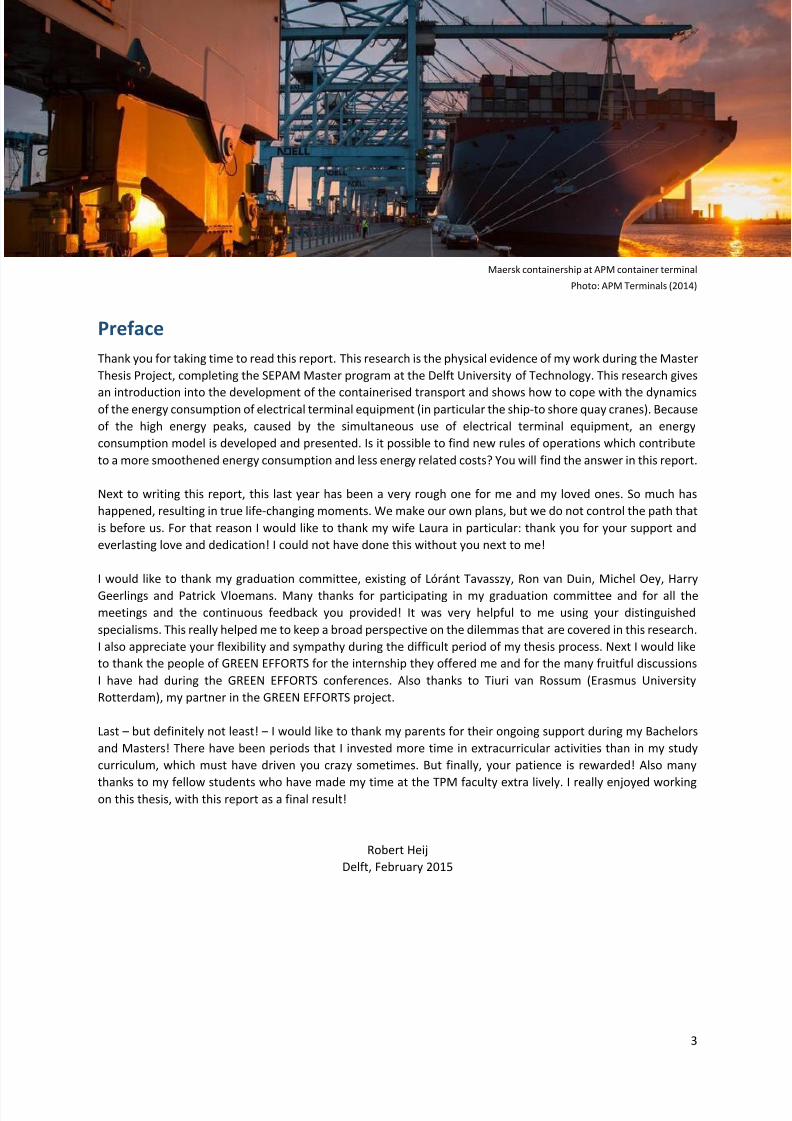
Maersk containership at APM container terminal
Photo: APM Terminals (2014)
Preface
Thank you for taking time to read this report. This research is the physical evidence of my work during the Master
Thesis Project, completing the SEPAM Master program at the Delft University of Technology. This research gives
an introduction into the development of the containerised transport and shows how to cope with the dynamicsof the energy consumption of electrical terminal equipment (in particular the ship-to shore quay cranes). Because
of the high energy peaks, caused by the simultaneous use of electrical terminal equipment, an energy
consumption model is developed and presented. Is it possible to find new rules of operations which contribute
to a more smoothened energy consumption and less energy related costs? You will find the answer in this report.
Next to writing this report, this last year has been a very rough one for me and my loved ones. So much has
happened, resulting in true life-changing moments. We make our own plans, but we do not control the path that
is before us. For that reason I would like to thank my wife Laura in particular: thank you for your support and
everlasting love and dedication! I could not have done this without you next to me!
I would like to thank my graduation committee, existing of Lóránt Tavasszy, Ron van Duin, Michel Oey, Harry
Geerlings and Patrick Vloemans. Many thanks for participating in my graduation committee and for all the
meetings and the continuous feedback you provided! It was very helpful to me using your distinguished
specialisms. This really helped me to keep a broad perspective on the dilemmas that are covered in this research.
I also appreciate your flexibility and sympathy during the difficult period of my thesis process. Next I would like
to thank the people of GREEN EFFORTS for the internship they offered me and for the many fruitful discussions
I have had during the GREEN EFFORTS conferences. Also thanks to Tiuri van Rossum (Erasmus University
Rotterdam), my partner in the GREEN EFFORTS project.
Last – but definitely not least! – I would like to thank my parents for their ongoing support during my Bachelors
and Masters! There have been periods that I invested more time in extracurricular activities than in my study
curriculum, which must have driven you crazy sometimes. But finally, your patience is rewarded! Also many
thanks to my fellow students who have made my time at the TPM faculty extra lively. I really enjoyed workingon this thesis, with this report as a final result!
Robert Heij
Delft, February 2015

7/23/2019 Thesis Robert Heij Final Digital Version
http://slidepdf.com/reader/full/thesis-robert-heij-final-digital-version 4/94
4
Stacking cranes at the port of Hong Kong.
Photo: Jonathan Brennan (Flickr, 1 October 2013)
Summary
The throughput of containers is growing yearly (World Shipping Council, 2011). At the same time the capacity of
containerships has grown from several hundreds of containers in the 1960s towards today’s 19,000 TEU1 carriers.
In order to achieve efficient operations of these large containerships, container carriers require high handlingspeeds and low handling costs when visiting container terminals. This development stimulated continuous
innovations at container terminals, resulting in growing automatisation of terminal operations.
Where minimisation of costs has always been a key performance indicator for terminals, over the last decade
the environmental performance has become another important performance indicator. This environmental
performance is enforced by governments and port organisations as well as carriers who demand less emissions
for handling their containers at a container terminal to improve the green image of their company and products.
In order to save costs and to reduce the greenhouse gas emission (especially CO 2) at container terminals, more
terminal equipment gets powered by more environment-friendly energy sources like biodiesel, hybrid systems
or electricity. Nowadays most modern container terminals are even fully electric. With a focus on higher handling
speeds, the peak capacity of terminal equipment (i.e. number of terminal equipment that are operating at the
same moment) increases. Because of the high price that is paid for the highest observed peak demand (leadingup to 20-30% of the terminals’ energy bill), it is beneficial to keep the peak demand as low as possible to reduce
the handling costs.
To investigate the opportunities for container terminals to reduce their peak demand, an energy consumption
model is developed to visualise the energy consumption of terminal equipment at container terminals. The
energy consumption model visualises the energy demand (kW/s) by focussing on the different movements that
are executed by terminal equipment. This focus is important, since the energy consumption differs per
movement. Hoisting a container consumes up to ten times more energy than a horizontal gantry movement.
Based on the energy consumption model a simulation model is developed to test rules of operation (i.e. changes
to the business operational procedures) that reduce the peak demand of terminals. Two rules of operation are
tested to analyse their effect on peak demand and handling time:
1) limiting the number of simultaneously lifting quay cranes;2) limiting the maximum energy demand per second.
The potential reduction in peak demand is around 50% against an extra handling time of less than half a minute
per hour. This can be achieved by reducing the maximum energy demand by 50%. By reducing the number of
simultaneously lifting quay cranes the peak demand decreases up to 40%, which is lower than for limiting the
energy demand per second. In this case the impact on terminal operations is also bigger, which makes it a less
optimal solution.
When reducing the peak demand by 50%, a container terminal with eight quay cranes is able to reduce their
peak related energy costs with about €249,000 per year; a major potential saving for container terminals, which
shows the opportunity for peak shaving the electricity demand at container terminals.
1 Twenty-foot equivalent unit (TEU) is a standardised unit which is used worldwide to measure the capacity of container
transport modalities (mostly ships) and throughput of containers (mostly at ports and terminals).
7/23/2019 Thesis Robert Heij Final Digital Version
http://slidepdf.com/reader/full/thesis-robert-heij-final-digital-version 5/94
5
Content
LIST OF FIGURES ............................................................................................................................................... 6
LIST OF TABLES ................................................................................................................................................. 7
ABBREVIATIONS ............................................................................................................................................... 7
1. INTRODUCTION ....................................................................................................................................... 8 1.1 DEVELOPMENT OF CONTAINERISED TRANSPORT ................................................................................................ 9
1.2 REDUCTION OF GREENHOUSE GASES ............................................................................................................. 12
1.3 PRICING OF ELECTRICITY ............................................................................................................................. 14
1.4 RESEARCH DESIGN .................................................................................................................................... 15
1.5 RESEARCH METHODOLOGY ......................................................................................................................... 17
1.6 CONCLUSION ........................................................................................................................................... 18
2. CONTAINER TERMINAL OPERATIONS ..................................................................................................... 19
2.1 EXPLORATION OF TERMINAL PROCESSES ........................................................................................................ 19
2.2 ENERGY CONSUMPTION OF CONTAINER TERMINALS ......................................................................................... 22
2.3 DYNAMICS IN ELECTRICAL ENERGY CONSUMPTION ........................................................................................... 25
2.4 RULES OF OPERATION ................................................................................................................................ 25
2.5 KNOWLEDGE GAP ..................................................................................................................................... 26
2.6 CONCLUSION ........................................................................................................................................... 27
3. ENERGY CONSUMPTION MODEL ............................................................................................................ 28
3.1 DEVELOPMENT OF CONSUMPTION MODEL ..................................................................................................... 28
3.2 DATA REQUIREMENTS ................................................................................................................................ 34
3.3 DEVELOPMENT OF SIMULATION MODEL .............................................................. ........................................... 35
3.4 DESCRIPTION OF SIMULATION MODEL ........................................................................................................... 40
3.5 MODEL VALIDATION .................................................................................................................................. 43
3.6 CONCLUSION ........................................................................................................................................... 45
4. EVALUATION OF PEAK SHAVING OPPORTUNITIES ................................................................................. 47
4.1 LIMITING SIMULTANEOUSLY LIFTING QUAY CRANES .......................................................................................... 47
4.2 LIMITING MAXIMUM ENERGY DEMAND ......................................................................................................... 51
4.3 ANALYSIS OF RESULTS ................................................................................................................................ 56
4.4 IMPLICATIONS OF RESULTS .......................................................................................................................... 57
4.5 CONCLUSION ........................................................................................................................................... 58
5. CONCLUSIONS AND RECOMMENDATIONS ............................................................................................. 59
5.1 CONCLUSIONS .......................................................................................................................................... 59
5.2 RECOMMENDATIONS ................................................................ ............................................................... .. 61
5.3 DIRECTIONS FOR FUTURE RESEARCH ............................................................................................................. 62
6. REFLECTION ........................................................................................................................................... 63
REFERENCES ................................................................................................................................................... 65
APPENDIX A: IDEF0 PROCESS SCHEMES .......................................................................................................... 69
APPENDIX B: LIST OF REQUIRED DATA FOR CONSUMPTION MODEL .............................................................. 76
APPENDIX C: IDEF0 PROCESS SCHEMES FOR (UN)LOADING CONTAINERS ...................................................... 77
APPENDIX D: ARRIVAL SCHEME CONTAINERSHIPS ......................................................................................... 79
APPENDIX E: RESULTS VERIFICATION AND SENSITIVITY ANALYSIS ................................................................. 80
APPENDIX F: RESULTS SIMULATION MODEL ................................................................................................... 81
APPENDIX G: PAPER ....................................................................................................................................... 84

7/23/2019 Thesis Robert Heij Final Digital Version
http://slidepdf.com/reader/full/thesis-robert-heij-final-digital-version 6/94
6
List of Figures
Figure 1: Visualisation of relation between reducing the handling time and higher handling costs. ..................... 9
Figure 2: Growth of largest containerships available (by mid-2014). ................................................................... 10
Figure 3: MSC Oscar (capacity: 19,226 TEU), shortly after its christening ............................................................ 10
Figure 4: Overview of HHLA container terminal in Hamburg. .............................................................................. 11
Figure 5: Position of European container ports in worldwide top-50 (2013) ....................................................... 11
Figure 6: Test calculation of Stedin (2014) ............................................................................................................ 15 Figure 7: Research flow diagram with main research processes (white) and data input (coloured) .................... 17
Figure 8: General process outline for handling containers at container terminals .............................................. 19
Figure 9: Schematic side-view on container terminal operations ........................................................................ 20
Figure 10 and 11 : A twin lift spreader (left) with a capacity of two 20 ft. containers and a tandem lift (right) with
a capacity of two 40 ft. containers. ....................................................................................................................... 21
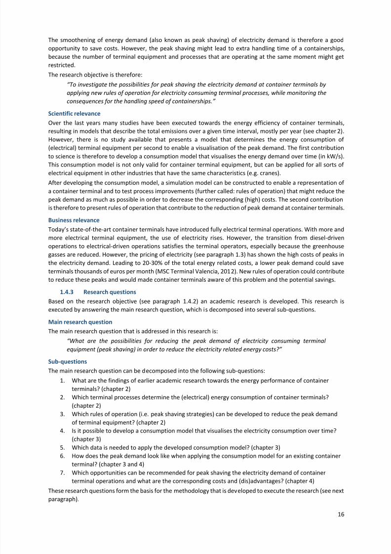
Figure 12: Conceptual model for determining energy consumption of terminal equipment .............................. 24
Figure 13: Overview of electricity usage at Noatum Container Terminal in Valencia .......................................... 24
Figure 14: Energy demand container terminal during one week (ABB, 2014). ..................................................... 25
Figure 15: IDEF0 process scheme ......................................................... ............................................................... .. 29
Figure 16: A0 scheme of container terminal .............................................................. ........................................... 29
Figure 17: Energy consumption of quay crane over time interval of eight minutes. ............................................ 31
Figure 18: Conceptualisation for determining energy consumption over time interval of movement ................ 32
Figure 19: Consumption model for determining the energy consumption per second ....................................... 33
Figure 20: Characteristics of different approaches, ordered by abstraction ........................................................ 36
Figure 21: Super post panamax quay cranes at MSC Terminal in Valencia. ......................................................... 37
Figure 22: Distribution of energy consumption (kWh) of MSCTV (2012) ............................................................. 37
Figure 23: Energy demand for handling a container with and without sub-movements (ABB, 2014) ................. 38
Figure 24: Overview of inputs and outputs simulation model ...................................................... ........................ 39
Figure 25: Main processes of simulation model ................................................................................................... 41
Figure 26: 3D screenshot of simulation model, running for an 8-crane terminal. ................................................ 41
Figure 27: 2D-screenshot of simulation model, running for an 8-crane terminal. ............................................... 42
Figure 28: Frequency graph for energy demand (measured per 0.1s) ................................................................. 44
Figure 29: Relation between peak demand and handling time (for 8-crane terminal) ........................................ 49 Figure 30: Potential savings per year for reducing number of lifting quay cranes ............................................... 49
Figure 31: Percentage of delayed containers by reducing lifting quay cranes ..................................................... 50
Figure 32: Average waiting time for delayed containers ...................................................................................... 50
Figure 33: Savings per second extra handling time. ............................................................................................. 50
Figure 34: Relation between peak demand and handling time when restricting energy demand for 8-crane
terminal ................................................................................................................................................................. 53
Figure 35: Potential savings per year for restricting maximum energy demand .................................................. 54
Figure 36: Percentage of delayed containers when restricting the energy demand ............................................ 54
Figure 37: Average waiting time for delayed containers ...................................................................................... 54
Figure 38: Savings per second extra handling time. ............................................................................................. 55
Figure 39: Frequency graph for energy demand during operations (measured per 0.1s) .................................... 60

7/23/2019 Thesis Robert Heij Final Digital Version
http://slidepdf.com/reader/full/thesis-robert-heij-final-digital-version 7/94
7
List of Tables
Table 1: Possible sequences for transporting containers on terminals ................................................................ 30
Table 2: Overview of required terminal equipment per process .......................................................................... 30
Table 3: Possible movements of terminal equipment .......................................................................................... 31
Table 4: Comparison of modelling approaches .......................................................... ........................................... 36
Table 5: Validation for energy demand of simulation model ............................................................................... 44
Table 6: Weighted difference for difference in energy demand........................................................................... 45 Table 7: Scenarios for limiting the lifting of quay cranes ...................................................................................... 47
Table 8: Effect of limiting the number of lifting quay cranes for 8-crane terminal .............................................. 48
Table 9: Effect of limiting the number of lifting quay cranes for 6-crane terminal .............................................. 48
Table 10: Best scoring scenarios based on impact on handling time and savings per second ............................. 51
Table 11: Scenarios for limiting the maximum energy demand for quay cranes ................................................. 52
Table 12: Effect of limiting the maximum energy demand for 8-crane terminal ................................................. 52
Table 13: Effect of limiting the maximum energy demand for 6-crane terminal ................................................. 53
Table 14: Best scoring scenarios based on impact on handling time and savings per second ............................. 56
Table 15: Cost containership per year, hour and second ..................................................................................... 57
Table 16: Optimal results for limiting number of simultaneously lifting quay cranes .......................................... 60
Table 17: Optimal results for limiting maximum energy demand ........................................................................ 61
Table 18: Arrival scheme with number of containers per containership ............................................................ .. 79
Table 19: Validation for distribution of containers per container load ................................................................ 80
Table 20: Detailed results for limiting number of simultaneously lifting quay cranes at 8-crane terminal .......... 81
Table 21: Detailed results for limiting number of simultaneously lifting quay cranes at 6-crane terminal .......... 81
Table 22: Detailed results for limiting maximum energy demand at 8-crane terminal ........................................ 82
Table 23: Detailed results for limiting maximum energy demand at 6-crane terminal ........................................ 83
Abbreviations
AGV Automated Guided Vehicles
ASC Automated Stacking Cranes
FEU Forty-foot equivalent unit, a sometimes used unit for presenting the capacity of ships and
container terminals in containers of 40 ft.
HDV Heavy Duty Vehicle
IDEF Integrated DEFinition
MSCTV MSC Terminal Valencia
NCTV Noatum Container Terminal Valencia
RMGC Rail-mounted Gantry Cranes (also referred to as ASC)
RTGC Rubber-tired Gantry Cranes
TEU Twenty-foot equivalent unit, a standard size for presenting the capacity of ships and container
terminals in containers of 20 ft. (40ft. container is 2 TEU)
TOS Terminal Operation System
7/23/2019 Thesis Robert Heij Final Digital Version
http://slidepdf.com/reader/full/thesis-robert-heij-final-digital-version 8/94
8
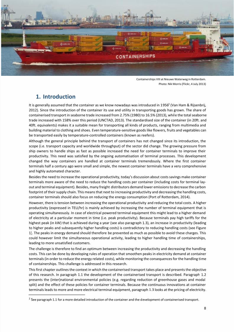
Containerships VIII at Nieuwe Waterweg in Rotterdam.
Photo: Nik Morris (Flickr, 4 July 2013)
1. Introduction
It is generally assumed that the container as we know nowadays was introduced in 19562 (Van Ham & Rijsenbrij,
2012). Since the introduction of the container its use and utility in transporting goods has grown. The share of
containerised transport in seaborne trade increased from 2.75% (1980) to 16.5% (2013), while the total seabornetrade increased with 158% over this period (UNCTAD, 2013). The standardised size of the container (in 20ft. and
40ft. equivalents) makes it a suitable mean for transporting all kinds of products, ranging from multimedia and
building material to clothing and shoes. Even temperature-sensitive goods like flowers, fruits and vegetables can
be transported easily by temperature-controlled containers (known as reefers).
Although the general principle behind the transport of containers has not changed since its introduction, the
scope (i.e. transport capacity and worldwide throughput) of the sector did change. The growing pressure from
ship owners to handle ships as fast as possible increased the need for container terminals to improve their
productivity. This need was satisfied by the ongoing automatisation of terminal processes. This development
changed the way containers are handled at container terminals tremendously. Where the first container
terminals half a century ago were small and simple, the newest container terminals have a very comprehensive
and highly automated character.
Besides the need to increase the operational productivity, today’s discussion about costs savings make container
terminals more aware of the need to reduce the handling costs per container (including costs for terminal lay-
out and terminal equipment). Besides, many freight distributors demand lower emissions to decrease the carbon
footprint of their supply chain. This means that next to increasing productivity and decreasing the handling costs,
container terminals should also focus on reducing the energy consumption (Port of Rotterdam, 2014).
However, there is tension between increasing the operational productivity and reducing the total costs. A higher
productivity (expressed in TEU/hr) is mainly achieved by increasing the number of terminal equipment that is
operating simultaneously. In case of electrical powered terminal equipment this might lead to a higher demand
of electricity at a particular moment in time (i.e. peak productivity). Because terminals pay high tariffs for the
highest peak (in kW) that is achieved during a year (see also paragraph 1.3), an increase in productivity (leading
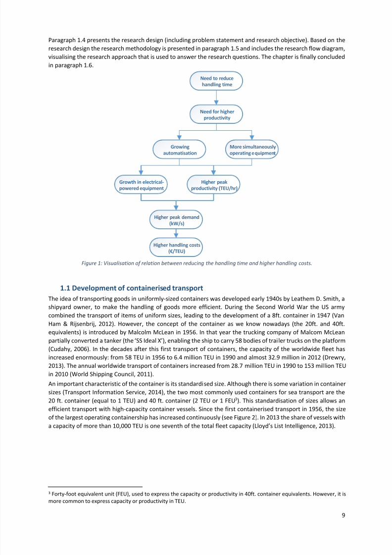
to higher peaks and subsequently higher handling costs) is contradictory to reducing handling costs (see Figure
1). The peaks in energy demand should therefore be prevented as much as possible to avoid these charges. Thiscould however limit the simultaneous operational activity, leading to higher handling time of containerships,
leading to more unsatisfied customers.
The challenge is therefore to find an optimum between increasing the productivity and decreasing the handling
costs. This can be done by developing rules of operation that smoothen peaks in electricity demand at container
terminals (in order to reduce the energy related costs), while monitoring the consequences for the handling time
of containerships. This challenge is addressed in this research.
This first chapter outlines the context in which the containerised transport takes place and presents the objective
of this research. In paragraph 1.1 the development of the containerised transport is described. Paragraph 1.2
presents the (inter)national environmental policies (e.g. regarding reduction of greenhouse gases and modal
split) and the effect of these policies for container terminals. Because the continuous innovations at container
terminals leads to more and more electrical terminal equipment, paragraph 1.3 looks at the pricing of electricity.
2 See paragraph 1.1 for a more detailed introduction of the container and the development of containerised transport.
7/23/2019 Thesis Robert Heij Final Digital Version
http://slidepdf.com/reader/full/thesis-robert-heij-final-digital-version 9/94
9
Paragraph 1.4 presents the research design (including problem statement and research objective). Based on the
research design the research methodology is presented in paragraph 1.5 and includes the research flow diagram,
visualising the research approach that is used to answer the research questions. The chapter is finally concluded
in paragraph 1.6.
Need to reduce
handling time
Need for higher
productivity
Growing
automatisation
Growth in electrical-
powered equipment
Higher peak
productivity (TEU/hr)
Higher handling costs
(€/TEU)
More simultaneously
operating equipment
Higher peak demand
(kW/s)
Figure 1: Visualisation of relation between reducing the handling time and higher handling costs.
1.1
Development of containerised transportThe idea of transporting goods in uniformly-sized containers was developed early 1940s by Leathem D. Smith, a
shipyard owner, to make the handling of goods more efficient. During the Second World War the US army
combined the transport of items of uniform sizes, leading to the development of a 8ft. container in 1947 (Van
Ham & Rijsenbrij, 2012). However, the concept of the container as we know nowadays (the 20ft. and 40ft.
equivalents) is introduced by Malcolm McLean in 1956. In that year the trucking company of Malcom McLean
partially converted a tanker (the ‘SS Ideal X’), enabling the ship to carry 58 bodies of trailer trucks on the platform
(Cudahy, 2006). In the decades after this first transport of containers, the capacity of the worldwide fleet has
increased enormously: from 58 TEU in 1956 to 6.4 million TEU in 1990 and almost 32.9 million in 2012 (Drewry,
2013). The annual worldwide transport of containers increased from 28.7 million TEU in 1990 to 153 million TEU
in 2010 (World Shipping Council, 2011).
An important characteristic of the container is its standardised size. Although there is some variation in container
sizes (Transport Information Service, 2014), the two most commonly used containers for sea transport are the
20 ft. container (equal to 1 TEU) and 40 ft. container (2 TEU or 1 FEU3). This standardisation of sizes allows an
efficient transport with high-capacity container vessels. Since the first containerised transport in 1956, the size
of the largest operating containership has increased continuously (see Figure 2). In 2013 the share of vessels with
a capacity of more than 10,000 TEU is one seventh of the total fleet capacity (Lloyd’s List Intelligence, 2013).
3 Forty-foot equivalent unit (FEU), used to express the capacity or productivity in 40ft. container equivalents. However, it is
more common to express capacity or productivity in TEU.

7/23/2019 Thesis Robert Heij Final Digital Version
http://slidepdf.com/reader/full/thesis-robert-heij-final-digital-version 10/94
10
Figure 2: Growth of largest containerships available (by mid-2014).
Source: Rodrigue (Hofstra University, 2012).
It is foreseen that the growth in container ship sizes will not come to an end soon. In 2014, Maersk introduced
the Triple-E ships, with a capacity of 18,000 TEU the largest operating containerships at that time (Maersk, 2013).
By the end of 2014 the Triple-E series were surpassed by the CSCL Globe and CSCL Pacific Ocean, with a capacity
of 19,100 TEU (Lloyds List, 2014). January 2015 the MSC Oscar was christened, with a capacity of 19,226 TEU
(MSC, 2014). In the future the maximum capacity is expected to increase even more: STX Shipbuilding developed
a 22,000 TEU containership (STX Shipbuilding, 2008) and the G6, a collaboration of six major container carriers,
is planning for 23,000 TEU containerships (Shippingwatch, 2014). David Tozer, Container Segment Manager at
Lloyd's Register is even expecting ships with a capacity of 24,000 TEU (ShippingWatch, 2014).
Figure 3: MSC Oscar (capacity: 19,226 TEU), shortly after its christening
(source: Daewoo Shipbuilding)
1.1.1
Handling of containers
A major advantage of the standardisation of containerised transport is the opportunity to facilitate intermodal
transport. Barges, trains and trucks enable the inland transport of containers between sea port container
terminals and its hinterland. Container terminals are therefore not only responsible for handling large
containerships, but also for transhipping containers from and to barges, trucks and trains.
A common layout for modern container terminals can be seen in Figure 4. On the water side of the terminal
(upper side of Figure 4) ship-to-shore quay cranes are responsible for handling containers between ship and
terminal. The stacks, where containers are stored while wait ing for further transhipment, are located behind the
quay cranes. The stacking of containers is one of the most challenging processes for terminal operators because
most containers have different origin-destination routes and are in need of different types of transhipment (i.e.
from truck/train to ship, ship to truck/train or ship to ship). Next to that, the storage period at the terminal also
differs for each container. The challenge is to have each container positioned on top of a stack when needed for
transport in order to prevent unproductive moves. On the land side of the terminal (downside of Figure 4) the

7/23/2019 Thesis Robert Heij Final Digital Version
http://slidepdf.com/reader/full/thesis-robert-heij-final-digital-version 11/94
11
containers are transported between the stacking area and arriving/departing trucks and trains. A detailed
explanation of the terminal processes is presented in chapter 2.
Most of the handled containers at container terminals are the standard dry containers, which are responsible for
89% of the containerised transport (World Shipping Council, 2013). The other 11% consists of reefers (used for
transport of temperature-controlled goods) and tank containers (used for transport of liquids). Special transport
(such as yachts and trucks) can also be transhipped on containerships, but this takes place rarely.
Figure 4: Overview of HHLA container terminal in Hamburg.
Source: ABB (2012)
1.1.2 Growth in container market
The number of worldwide handled containers increased continuously over the last decades, to 157 million TEU
in 2012 (Clarksons, 2014). Looking to the world’s largest container ports, Shanghai was world leader in 2012 with
32.53 million TEU (see Figure 5). Striking fact is that seven out of the ten largest container ports are located in
China. The first European port - the Port of Rotterdam - is ranked 11 th, closely followed by Hamburg (15th) and
Antwerp (16th
).
Figure 5: Position of European container ports in worldwide top-50 (2013)
Source: (World Shipping Council, 2014)
Compared to 2011, the number of handled containers of the 50 largest container ports has grown from 410
million TEU (2012) to 423 million TEU (2013), an increase of 3.1% (World Shipping Council, 2014). In 2012 the
total worldwide transport of containers increased by 3.8% to 601.8 million TEU (UNCTAD, 2013).
Due to the increasing size of containerships, growth in handled containers and growing competition, container
carriers demand higher handling speeds of their ships against lower prices per TEU (i.e. faster and cheaper). For
33,62 32,60
23,28 22,35
17,69 17,3315,52 15,31
13,64 13,01 11,629,30 8,59
5,84 4,50 4,33 3,74 3,09 2,75
0,00
10,00
20,00
30,00
40,00
T E U ( X M I L L I O N )
World's largest container ports (2013)

7/23/2019 Thesis Robert Heij Final Digital Version
http://slidepdf.com/reader/full/thesis-robert-heij-final-digital-version 12/94
12
container terminals, this leads to a continuous pressure to innovate. However, another driving factor of
innovations are the (inter)national policies aiming to reduce the emission of greenhouse gases and the increasing
availability of new (electrical) terminal equipment (more environment-friendly). These two aspects will be
discussed in the next paragraph.
1.2 Reduction of greenhouse gases
In designing and improving terminal operations, container terminals need to operate within the legal boundaries,determined by governments on local, national and international level. Over the last decades more and more
climate policies are unrolled, aiming to reduce greenhouse gas emissions. These policies directly affect container
terminal performances (via governments and port operators demanding lower emissions) and indirectly (via
container carriers and their customers who demand cleaner terminal operations to make their supply chain more
sustainable). Driven by these policies, container terminals are stimulated to seek opportunities to lower their
emissions. There are four main drivers for terminals to address the environmental impact of their operations
(Geerlings, 1999):
1. leaner operations (e.g. skipping non-necessary activities and looking for optimisations)
2. transport via less damaging modalities (modal shift from trucks to trains/barges)
3. using new technologies (e.g. automatisation of processes)
4. change of behaviour (e.g. implementing rules of operation to change existing processes)
This paragraph presents the environmental policies and corresponding goals and elaborates on some of the four
presented main drivers which contribute to a lower/better energy consumption.
1.2.1 Introduced climate policies
Over the last decades the issue of climate change gained a lot of attention. Although expert opinions differ on
the level of influence humans have on the climate change, the fact that the human environmental footprint
should be reduced gets worldwide consensus. In 1997, the United Nations adopted the Kyoto-protocol agreeing
to reduce greenhouse gases by 2012 with an average of 5.2% compared to 1990; fifteen EU member states
agreed to reduce their CO2-level by 2012 with an average of 8% (United Nations, 1997). By the end of 2012 the
Netherlands achieved a reduction of almost 10% (Compendium voor de Leefomgeving, 2013).
In 2012 an amendment to the Kyoto-protocol was adopted. In this amendment, new arrangements were made
on the greenhouse gas reduction of participating countries. The Dutch government agreed to reduce theiremissions with another 12% by 2020 (compared to 1990). This implies a total reduction of 20% between 1990
and 2020 (United Nations, 2012).
In addition to this worldwide agreement, the European Union offered to save another 10% (to 30% in total) if
other major economies would make a proportional effort in reducing their emissions (European Commission,
2014). The Dutch government again added another 10% in their climate agenda by advocating a CO 2-reduction
of 40% by 2030 (Ministerie van Infrastructuur & Milieu, 2013). The municipality of Rotterdam, provider of the
largest European port, adopted the Rotterdam Climate Initiative which plead for a CO2-reduction of 50% by 2025
(Rotterdam Climate Initiative, 2014).
1.2.2
Lowering emissions at container terminals
As introduced before, there are four main drivers for container terminals to address the issue of lowering
greenhouse gas emissions (Geerlings, 1999). These four main drivers are discussed below:
Leaner operations
A relative easy way to influence the terminal’s operations and its emissions is to analyse the terminal operations
and to skip non-necessary activities. This can be achieved in several ways (Froese, 2014):
- minimising travelling distances at terminals;
- adapting operations to actual needs (e.g. optimising driving speeds and equipment performances);
- reducing consumption of terminal equipment (e.g. switching terminal equipment from active to idle
state when possible and using more energy-friendly energy sources);
- optimising yard lighting (e.g. switching to LED and only illuminating necessary areas) and
- minimising energy consumption of reefers (e.g. sun-shading or temporarily turning-off power).
Results of research towards these subjects are discussed in paragraph 2.2.

7/23/2019 Thesis Robert Heij Final Digital Version
http://slidepdf.com/reader/full/thesis-robert-heij-final-digital-version 13/94
13
Modal shift
In 2012 the transport sector was responsible for 29% of the Dutch energy consumption and 32% of the European
energy consumption (Eurostat, 2012). To achieve the ambitious reduction of greenhouse gases, the transport
sector could not stay unaffected. When comparing three modes for inland transport (road, rail and inland water
transport), it is shown that the transport by barges and trains cause less pollution of CO2. Barges reduce the
emission (in kg. CO2 per ton/km) with 45% compared to trucks. For diesel trains this reduction is 60% (CE Delft,
2011). National governments are trying to increase the transport by barges and trains in order to establish a
reduction in CO2.
The share of each modality is represented by the modal split, a percentage that reveals the total transported
TEU*km per modality. In 2011 the modal split for the Netherlands I general was 49.3% by road, 44.6% by inland
water transport and 6.1% by rail (Eurostat, 2011). To shift this modal split towards more transport by trains and
barges, also known as modal shift, the European Union and Dutch government initiated several policies.
In their white paper on transport, the European Commission focused on a more sustainable transport system.
By 2030 almost 30% of the road transport over 300km should shift to rail or water transport. By 2050 this
percentage should be 50% (European Commission, 2011). To achieve a more sustainable port and especially to
unburden the road network, the Port of Rotterdam agreed with the new container terminals on Maasvlakte 2 to
change the modal split in the period until 2030. Compared with the modal split in 2012, the barge transport
should increase from 35.3% to 45.0% and the rail transport should increase from 10.7% to 20.0%. The goal for
road transport is to reduce the modal split from 54.0% to 35.0% (Port of Rotterdam, 2013). This modal shiftimplies serious effort for the twelve container terminals situated in the Port of Rotterdam to contribute to a
reduction in greenhouse gases.
Availability of new technologies
Another development that led to a reduction of emissions at container terminals is the use of more environment-
friendly energy sources by terminal equipment at container terminals. Where two decades ago most terminal
equipment was powered by diesel, nowadays more and more equipment is powered by less polluting sources
(e.g. biodiesel, hybrid systems or electricity4). This reduction of greenhouse gases goes hand in hand with
increasing productivity, as could be seen at the ECT and APM terminals in Rotterdam.
In 2000 ECT introduced diesel driven AGVs and automated stacking cranes (ASCs) on their terminal. Instead of
processing containers with straddle carriers, the AGVs led to a fully automated process without humaninteraction of drivers. The use of diesel was reduced because the equipment was driving more efficiently
compared with human drivers. Meanwhile innovation led to the introduction of hybrid AGVs, which were
introduced by ECT in 2012 (ECT, 2012). The next generation, fully electric AGVs, is announced by the new
container terminal of APM Terminals at Maasvlakte 2. By 2015 the newest generation of battery-powered AGVs
will be in operation (APM Terminals, 2012).
This example in the Port of Rotterdam shows the development of electrification that has been introduced in
almost all terminal processes, allowing the state of the art container terminals to be fully electrified. Although
the use of electricity is more environment-friendly, a challenge arises with regard to the way electricity is priced.
This dilemma is addressed in paragraph 1.3.
Change of behaviourA fourth driver is the change of behaviour at container terminals. New rules of operations, that change the
currently used steering processes, might contribute to costs and or energy savings. The question that is
addressed in this research – Is it possible to smoothen the energy demand by implementing new rules of
operations? – is a good example. By changing the behaviour, i.e. the way in which operations are used to be
executed, more awareness about the terminal operations can be achieved.
4 Despite some companies that state that the consumption of electricity (in kWh) is free of emissions, the production ofelectricity from renewable energy sources is only 4.4%. The major share is still derived from coal and gas, causing emission
at power plants (CBS, 2012).

7/23/2019 Thesis Robert Heij Final Digital Version
http://slidepdf.com/reader/full/thesis-robert-heij-final-digital-version 14/94
14
1.3 Pricing of electricity
Since more and more terminal processes are electrified, the electricity consumption of terminals rises. The
electricity related costs are made up of two aspects (Autoriteit Consument & Markt, 2013):
1) fixed costs for connecting the terminal to the power network and
2) variable costs related to the (predicted and actual) consumption of electricity.
The fixed costs for connecting a container terminal to the power network consist of the initial investment costs
for connecting the terminal to the power network and a yearly payment for the connection. The variable costsrelate to the contracted transmission capacity (€/kW/year), highest peak demand (€/kW/month) and actual
energy consumption (€/kWh).
1.3.1
Fixed costs
The hardware costs are fixed and determined by the electrical infrastructure of the terminal. The yearly costs
depend on the costs related to the type of connection that is needed. For container terminals there are two
feasible options: the so called ‘medium voltage’ (1-20 kV) and ‘between voltage’ (50/25 kV). A lower type of
connection is only used for consumers, who have a relatively low energy demand and the two higher types are
used for transporting electricity through the high voltage network (Autoriteit Consument & Markt, 2014). Out of
the two feasible options, most container terminals will request a ‘between voltage’ connection, since the
contractual transported supply is higher than 2,000 kW (Liander, 2014) (ABB, 2014).
1.3.2
Variable costs
Besides the fixed costs for enabling the terminal to receive electricity, there are three aspects that determine
the variable costs (Stedin, 2014).
1. The first aspect is the payment for actual energy demand (€/kWh/year) , which is determined by
measuring the actual power consumption over a certain period.
2. The second aspect are the transmission capacity costs. On forehand, container terminals need to present
the height of their power demand, the so called contracted transmission capacity ( ). This
demand is charged per year (€/kWd /). When the predetermined contracted demand
differs too much from the average actual demand, the electricity supplier will charge the costs based on
the actual demand.
3. The third aspect is then the charge for peak demand. The container terminals are charged for the highest
peak demand that is observed over a year ( mx ), even while this maximum is only achieved during a
fraction of a second. Officially the peak is charged per month, but the policy of the grid exploiters is to
charge peaks not only for the month in which it occurred, but to charge the peak for the next twelve
months. To illustrate this: if in January the highest peak is 2,000 kW, the terminal will have to pay 2,000
times the monthly tariff per kW for the rest of that year. However, if the highest peak in March is 2,500
kW, the payment will be adjusted to 2,500 the monthly tariff for the next twelve months, until February
the next year. In this way energy suppliers are charging companies for their peak demand because the
peak demand is almost always higher than the requested contractual demand (i.e. > ), which means that the energy suppliers could not prepare their energy production for this
extra demand. Although this does not lead to big problems (the energy supply in the Netherlands is almost
always sufficient to satisfy the energy demand), the energy suppliers do charge the unpredictable peaks.
1.3.3
Relevance for container terminals
Container terminals are able to influence the variable aspect of their monthly energy bill. Next to more energy
efficient measures that reduce the actual energy consumption in kWh, the main challenges for container
terminals are to achieve a steady power demand (enabling terminals to predict their contracted transmission
capacity more accurate) and to reduce their peak demand as much as possible (especially because the highest
peak is charged for the next twelve months). This lower peak demand will not lead to a lower total energy
consumption or lower emissions, but will only save costs due to the pricing of peak demand.
For a container terminal, the costs related to the peak demand can count up to 25% of the total energy bill of a
terminal (ABB, 2014). A standard test calculation of the Dutch grid operator Stedin (see Figure 6 on page 15),
shows a peak cost percentage of even 30% of the total energy bill. Stedin charges peaks for almost €27 per kW
per year (i.e. €2.2445 per kW/month), which shows the opportunity for container terminals to save costs when
their peak demand is reduced. Halving the peaks can reduce the total energy bill with approximately 12.5-15%,which yields a container terminals tens of thousands of euros per month (MSC Terminal Valencia, 2012).

7/23/2019 Thesis Robert Heij Final Digital Version
http://slidepdf.com/reader/full/thesis-robert-heij-final-digital-version 15/94
15
Figure 6: Test calculation of Stedin (2014)
1.4 Research design
1.4.1 Problem statement
The first paragraphs of this chapter described the development of the containerised transport and today’s
challenges for container terminals. Despite the economic crisis, terminals face a growing container market with
increasing capacities of containerships and growing competition between shipping companies. In order to satisfyshipping companies and to retain their competitive position, container terminals need to increase the handling
speed of containerships and minimise the corresponding costs (goal: cheaper and faster). On the other hand, the
propagated climate policies of several governments and port organisations challenge container terminals to
reduce their greenhouse gas emissions (goal: more environment-friendly). A ‘greener’ image is becoming more
and more important for terminals, since major companies (e.g. Walmart) are focussing on reducing the emissions
in their supply chain and are therefore requesting low emissions from the container carriers that are transporting
their goods and from the container terminal that is operating their containers (Port of Rotterdam, 2014).
Stimulated by the environmental policies of governments, the growing pressure from clients to increase handling
speeds and lower emissions, container terminals feel a growing need to innovate and become more efficient.
Over the last years, this led to the entrance of more and more electrical terminal equipment, which is not only
more efficient, but also more environment-friendly than the replaced diesel-driven equipment.
However, the high pressure of carriers to handle the containerships as fast as possible leads to more electrical-
driven terminal equipment that is operating at the same moment, potentially causing high peaks in energy
demand. Because the peak demand is charged separately (see paragraph 1.3), the peak-related costs are
responsible for 25-30% of the total electricity costs (ABB, 2014) (Stedin, 2014). This means that when the
requested higher handling speeds of ships are obtained by operating more terminal equipment at the same time,
this results in higher handling costs. Because carriers request both higher handling speeds and lower handling
costs, this means that terminals have to look for new rules of operation, which are able to reduce the peaks in
electricity demand while maintaining high handling speeds.
1.4.2 Research objective
The research objective describes the goal of the research and is derived from the problem statement in
paragraph 1.4.1. The focus on environment-friendly innovations leads towards more and more terminalequipment that is powered by electricity. However, the use of many electricity powered terminal equipment
causes peaks in energy demand when several energy intensive processes are executed at the same moment.
7/23/2019 Thesis Robert Heij Final Digital Version
http://slidepdf.com/reader/full/thesis-robert-heij-final-digital-version 16/94
16
The smoothening of energy demand (also known as peak shaving) of electricity demand is therefore a good
opportunity to save costs. However, the peak shaving might lead to extra handling time of a containerships,
because the number of terminal equipment and processes that are operating at the same moment might get
restricted.
The research objective is therefore:
“To investigate the possibilities for peak shaving the electricity demand at container terminals by
applying new rules of operation for electricity consuming terminal processes, while monitoring the
consequences for the handling speed of containerships.”
Scientific relevance
Over the last years many studies have been executed towards the energy efficiency of container terminals,
resulting in models that describe the total emissions over a given time interval, mostly per year (see chapter 2).
However, there is no study available that presents a model that determines the energy consumption of
(electrical) terminal equipment per second to enable a visualisation of the peak demand. The first contribution
to science is therefore to develop a consumption model that visualises the energy demand over time (in kW/s).
This consumption model is not only valid for container terminal equipment, but can be applied for all sorts of
electrical equipment in other industries that have the same characteristics (e.g. cranes).
After developing the consumption model, a simulation model can be constructed to enable a representation of
a container terminal and to test process improvements (further called: rules of operation) that might reduce thepeak demand as much as possible in order to decrease the corresponding (high) costs. The second contribution
is therefore to present rules of operation that contribute to the reduction of peak demand at container terminals.
Business relevance
Today’s state-of-the-art container terminals have introduced fully electrical terminal operations. With more and
more electrical terminal equipment, the use of electricity rises. However, the transition from diesel-driven
operations to electrical-driven operations satisfies the terminal operators, especially because the greenhouse
gasses are reduced. However, the pricing of electricity (see paragraph 1.3) has shown the high costs of peaks in
the electricity demand. Leading to 20-30% of the total energy related costs, a lower peak demand could save
terminals thousands of euros per month (MSC Terminal Valencia, 2012). New rules of operation could contribute
to reduce these peaks and would made container terminals aware of this problem and the potential savings.
1.4.3
Research questionsBased on the research objective (see paragraph 1.4.2) an academic research is developed. This research is
executed by answering the main research question, which is decomposed into several sub-questions.
Main research question
The main research question that is addressed in this research is:
“ What are the possibilities for reducing the peak demand of electricity consuming terminal
equipment (peak shaving) in order to reduce the electricity related energy costs?”
Sub-questions
The main research question can be decomposed into the following sub-questions:
1. What are the findings of earlier academic research towards the energy performance of container
terminals? (chapter 2)2. Which terminal processes determine the (electrical) energy consumption of container terminals?
(chapter 2)
3. Which rules of operation (i.e. peak shaving strategies) can be developed to reduce the peak demand
of terminal equipment? (chapter 2)
4. Is it possible to develop a consumption model that visualises the electricity consumption over time?
(chapter 3)
5. Which data is needed to apply the developed consumption model? (chapter 3)
6. How does the peak demand look like when applying the consumption model for an existing container
terminal? (chapter 3 and 4)
7. Which opportunities can be recommended for peak shaving the electricity demand of container
terminal operations and what are the corresponding costs and (dis)advantages? (chapter 4)
These research questions form the basis for the methodology that is developed to execute the research (see next
paragraph).

7/23/2019 Thesis Robert Heij Final Digital Version
http://slidepdf.com/reader/full/thesis-robert-heij-final-digital-version 17/94
17
1.5 Research methodology
1.5.1
Research approach
The research approach describes the methodologies that are used to answer the presented research questions
(see paragraph 1.4.3) in order to achieve the research objective. The research aims to gain more insight in the
peak demand for electrical terminal equipment. In general this research is made up of an extensive literature
study, the development of a consumption model and finally the development of a simulation model as a case
study to test new rules of operation that might reduce the peak demand at container terminals, leading torecommendations that contribute to the peak shaving of the electricity demand at container terminals. The
research approach is described more elaborately below.
After the introduction – which presents more understanding of the position of the containerised transport – the
problem statement is introduced. Based on the problem statement a research objective and research questions
are formulated. To gain a more detailed understanding of the problem, an extensive literature review is executed
towards the environmental policies, energy consumption of container terminals and relevant terminal processes.
This summarises earlier research and generates an overview of relevant processes that need to be included in
monitoring the energy demand of container terminals (sub-question 1 and 2). Also the potential rules of
operation that can be implemented to reduce the peak demand are presented (sub-question 3).
Based on the knowledge gap that is identified at the end of chapter 2, a consumption model is developed to
determine the energy demand (kW/s) of electrical-driven terminal processes. This creates a deeper insight in thevolatile energy consumption of container terminals and the data that is needed to represent this energy
consumption over time (sub-question 4 and 5). The relevant processes of the consumption model are then
applied in a case study for an existing container terminal. Due to the dynamic aspect of the energy consumption
and the need to test new rules of operation that might contribute to lowering the peak demand, a simulation
model will be constructed for this purpose.
After the model has been validated with real data and expert opinion, the model can be used to test the earlier
developed rules of operation (sub-question 6 and 7). For every new rule, the advantages and disadvantages are
presented, resulting in conclusions that show which (combination of) rules of operation are most effective and
feasible. The research is finally concluded by giving recommendations and directions for further research and by
reflecting on the current research.
1.5.2
Thesis outlineThe thesis outline is visualised by a research flow diagram (see Figure 7). The research flow diagram visualises
the research process and shows the steps where literature, expert opinion and/or data is needed (Verschuren &
Doorewaard, 2010). The white blocks represent the main processes, from problem statement to conclusions and
recommendations. The coloured blocks serve as input for several processes and represent the needed sources.
The diagram can be seen as thesis outline, considering the fact that the steps are categorised per chapter.
Introduction and research outline
Chapter 1
Extended research
on research
objective
Research objective
and research
questions (§1.4)
Detailed
understanding of
problem (§2.1-2.4)
Energy consumption model
Chapter 3
Development of
consumption model
(§3.1-3.2)
Evaluation of peak shaving opp ortunities
Chapter 4
Validation of
simulation model
(§3.5)
Conclusions and recommendations
Chapter 5
Reflection
Chapter 6
Conclusions and
recommendations
(§5.1-5.3)
General research on
containerised
transport
Problem statement
(§1.4)
Existing studies
towards energy
consumption
container terminals
Development of
simulation model
(§3.3-3.4) Data from container
terminals and expertopinion
Results and
implications rules of
operation (§4.1-4.4)
Knowledge gap
(§2.5)
Introduction of
research topic
(§1.1-1.3)
Identifying knowledge gaps
Chapter 2
Research
methodology (§1.5)
Reflection on
research
(Ch. 6)
Figure 7: Research flow diagram with main research processes (white) and data input (coloured)

7/23/2019 Thesis Robert Heij Final Digital Version
http://slidepdf.com/reader/full/thesis-robert-heij-final-digital-version 18/94
18
1.6 Conclusion
The growing size of containerships and increasing annual worldwide transport of containers has stimulated
container terminals to make their processes more efficient and to focus on higher handling speeds and lower
handling costs. Stimulated by governmental policies aiming to reduce the greenhouse gas emissions (mainly
focused on CO2), more and more electrical-powered terminal equipment is introduced. Although the total
emissions are reduced by this development, a dilemma occurs when the need to increase handling speeds leads
to more simultaneously operating terminal equipment and higher peaks in electricity demand. Because of the
charged costs for these energy peaks – leading to 25-30% of the total energy bill (ABB, 2014) (Stedin, 2014),
peaks have to be prevented as much as possible.
An energy-related cost reduction for a container terminal might lead to an increased handling time of a
containership. When applying new rules of operation that reduce the peak demand, the trade-off between the
(higher) handling time of a containership and the (lower) costs related to a lower peak demand has to be
monitored in order to weigh the effects of both performance indicators.
In order to investigate the peak demand at container terminals, more insight is needed into the terminal
processes and corresponding energy-consuming elements. This question is addressed in chapter 2.

7/23/2019 Thesis Robert Heij Final Digital Version
http://slidepdf.com/reader/full/thesis-robert-heij-final-digital-version 19/94
19
Containership ZIM Rotterdam entering the Yangtze port in Rotterdam
Photo: Hans Elbers (Fotovlieger.nl, 23 February 2014)
2. Container terminal operations
The main research question (presented in chapter 1) suggests to develop an energy consumption model that can
be used to visualise the energy consumption of a container terminal over time and which forms the basis for a
simulation model that enables the testing of newly developed rules of operation to reduce the peaks in electricitydemand at container terminals. But in order to develop such a consumption model, first more understanding is
needed about the operations and energy consumption of container terminals.
This chapter starts with an exploration towards the terminal processes to get a broader understanding of the
operations that take place at a container terminal (paragraph 2.1). After that, paragraph 2.2 discusses earlier
(scientific) studies towards the sustainability of container terminals. In paragraph 2.3 the volatility of a terminals’
energy demand is visualised, followed by the development of rules of operation that contribute to a lower peak
demand (paragraph 2.4). These first four paragraphs lead to the formulation of the knowledge gap in paragraph
2.5. The chapter is concluded in paragraph 2.6.
2.1 Exploration of terminal processes
In order to get a more comprehensive view on the energy consumption of container terminal, the generalterminal operation will be decomposed into processes to enable a better understanding of all (energy-
consuming) movements at terminals, which increases insight in all elements that influence the energy
consumption. The container handling processes at terminals are described by inter alia Vis & De Koster (2003),
who give an overview of all processes related to the transhipment of containers at container terminals. In general
six handling processes can be distinguished: the arrival of the ship, (un)loading of the ship, transport of containers
between stacking area and quay cranes, (un)stacking of containers, inter-terminal transport and other modalities
(see Figure 8 and Figure 9). These six processes are described in paragraphs 2.1.1-2.1.6. In paragraph 2.1.7 the
remaining terminal processes are described shortly.
Figure 8: General process outline for handling containers at container terminals
Source: (Vis & De Koster, 2003)

7/23/2019 Thesis Robert Heij Final Digital Version
http://slidepdf.com/reader/full/thesis-robert-heij-final-digital-version 20/94
20
Figure 9: Schematic side-view on container terminal operations
Source: (Steenken, Voß, & Stahlbock, 2004)
2.1.1 Arrival of the ship
Before the ship arrives, the terminal must reserve a berthing place for the handling time that is expected for the
incoming containership. Based on the vessel attributes of incoming ships (vessel code, length, depth and width)
and handling plan (pre-arrival and pre-departure time, expected number of handled containers and expected) a
berthing place is allocated (Sun, Sun, & Yang, 2009). The allocation of berthing places can be done in different
ways. One strategy is to minimize the time ships are docked at the quay side. Containers are then handled by the
‘first come first serve’ principle. Another strategy would be to moor a ship close to the stacking area where most
of the containers are located that need to be loaded on this ship. Despite the beneficial influence on the
minimisation of total transport distance of containers, this strategy could be detrimental for the average waiting
time which will likely dissatisfy container carriers (Imai, Nagaiwa, & Tat, 1997).
2.1.2 (Un)loading of containers
After the ship has been moored, the quay cranes and barge cranes are able to unload the incoming containers
based on the unloading plan. For loading and unloading containers, ship-to-shore cranes (or barge cranes in case
of barges) are used. Quay cranes usually use a normal spreader for transferring a container, which enables them
to handle one container at the same time. Quay cranes which possess a more advanced spreader can handle
more containers at the same time (e.g. the twin-lift and tandem-lift) (Stahlbock & Voß, 2008). The Super Post
Panamax quay cranes, the currently standard cranes for unloading the largest containerships, are able to make
approximately 32 lifts per quay crane per hour (APM Terminals, 2014). This allows a quay crane to handle 32-64
TEU per hour with a normal spreader and up to 128 TEU per hour with a tandem lift spreader.
The handling capacity of a container terminal is highly dependent on the number of quay cranes and their
capacity, because the cranes determine the handling time for a ship as well as the throughput of containers to
the stacking process (Eugen, Şerban, Augustin, & Ştefan, 2014).
During the (un)loading of a containership (i.e. stowage), two criteria are important: the ship’s stability and
number of unproductive moves (Imai, Sasaki, Nishimura, & Papadimitriou, 2006) . While (un)loading, the ship’sstability changes due to the continuously changing container load. Because containerships visit several container
terminals, each of them unloading containers from and loading containers to the ship, not all containers which
have to be unloaded are positioned on top of the ship’s stacks. The ships have therefore to be loaded in an
efficient way, allowing the next container terminal to unload them with a minimum of unproductive moves.
These two criteria are often in conflict, because the most efficient loading (regarding the minimisation of
unproductive moves) might not also be in line with the most efficient loading regarding the ship’s stability. This
makes the stowage very complex (Bortfeldt & Gehring, 2001) (Steenken, Voß, & Stahlbock, 2004) (Dekker, Voogd,
& Van Asperen, 2006), especially because the stowage plans have to be aligned over all different ports that have
to (un)load the ship (Wilson & Roach, 2000).
Quay cranes are connected to the electricity network. For all quay crane processes (moving of crane and
spreader, crane lighting and auxiliary processes) electricity is supplied by the network. For the lowering of a
container power is even regenerated and returned to the power network. However, the energy consumption for

7/23/2019 Thesis Robert Heij Final Digital Version
http://slidepdf.com/reader/full/thesis-robert-heij-final-digital-version 21/94
21
lifting a container is higher than for other crane movements (see chapter 3.3 for a more detailed description of
this energy demand).
Figure 10 and 11 : A twin lift spreader (left) with a capacity of two 20 ft. containers
and a tandem lift (right) with a capacity of two 40 ft. containers.
Source: Port Strategy (2007 & 2009).
2.1.3 Transport of containers
The third process is the transport of containers between the stacking area and quay cranes. First, incomingcontainers are unloaded from the ship and then placed on a vehicle on the land side, which brings the container
to the right stacking row in which the container later will be placed. For this transport several types of equipment
are deployed (e.g. automated guided vehicles, reach stackers, terminal trucks or straddle carriers), with different
energy consumption specifications. AGVs are driven by diesel, hybrid systems or fully electric via batteries. The
current terminal trucks, straddle carriers and reach stackers run on (bio)diesel. In the future these types of
equipment might also be available on fully electric. The determination which type of transport is used and how
many vehicles are needed to handle the daily operations is important for terminals (Vis & De Koster, 2003),
because too much equipment increases the equipment costs for container terminals and insufficient equipment
increases the handling time for container carriers.
2.1.4 Stacking of containers
Containers arrive at the stacking area at so called input/output points, I/Os, where containers enter the stackingarea from the quay side and landside or leave the stacking area to one of these sides (Carlo, Vis, & Roodbergen,
2014). Based on a survey of 113 container terminals worldwide, the most frequently used stacking cranes are
the rubber-tired gantry cranes (RTGCs, 63%), straddle carriers (20%) and rail-mounted gantry cranes (RMGCs,
6%) (Wiese, Kliewer, & Suhl, 2009). The RTGCs are mainly seen in Asia, where the straddle carriers and RMGCs
are mostly used in Europe. The RMGCs are currently known as automated stacking cranes (ASCs), which operate
without human interaction (Carlo, Vis, & Roodbergen, 2014). RTGCs run on diesel and have a generator to
convert diesel to electricity for controlling the spreader. The ASCs are connected to the electricity network, just
as the quay cranes.
Restacking
Besides the stacking activities of incoming and outgoing containers, containers are also moved to another stack
to support a smooth loading and unloading of containers. This is the case when for example a container which is
stacked below another container is needed first. Then the above piled container(s) can be restacked to enable a
smoother transport of the needed container. Each move that is made to release a lower stacked container is
called an unproductive move. Container terminals try to minimise the number of unproductive moves because
these movements are time-consuming and costly without having a directly added-value.
Reefers
Temperature-controlled containers, known as reefers, are placed in special parts of the stacking area where
electricity plugs are available. The reefers are (un)plugged manually by reefer mechanics. The method which is
used to build this schedule has a major influence on the productivity of the reefer mechanic (Hartman, 2012). In
general the reefer mechanic receives a job from the terminal operation system (TOS). The mechanic walks or
drives to the specified reefer stack and (un)plugs the container, after which the mechanic confirms the
completion of the job so the TOS knows that the mechanic is available. The challenge is to balance the minimised
weighted sum of idle time and total travel time (Hartman, 2012).

7/23/2019 Thesis Robert Heij Final Digital Version
http://slidepdf.com/reader/full/thesis-robert-heij-final-digital-version 22/94
22
Because of the fixed position of the reefer stacks, the terminal operations are highly influenced by the size and
position of the reefer stacks. After testing several terminal layouts (including reefer stacks) the distribution of
reefer stacks over the whole stacking area of a terminal was proven to be more efficient than the currently used
centralised layout, where all reefers are stacked together (Choi, et al., 2004).
2.1.5 Inter-terminal transport
The inter-terminal is also known as the landside transport and deals with the transport between the stacks and
the loading area for trucks or trains (see Figure 9, page 19). This transport can be executed by multi-trailer trucks(which are able to transport multiple containers at once) or AGVs, but also by straddle carriers or reach stackers,
depending on the loading process of containers on trucks and trains. When there is a separate crane terminal for
(un)loading these modalities, the containers need to be transported to the cranes in order to be picked up and
loaded on the train. This can be done with multi-trailer trucks or AGVs. For using multi-trailer trucks, the
challenge is to minimise the number of empty trips and trailers (Vis & De Koster, 2003).
If no separate (un)loading terminal exists, the containers can be picked up at the stacks with equipment that is
able to load the trucks and trains, or vice versa. This can be done with for example straddle carriers and reach
stackers.
Next to the transport between the trucks/trains and stacking area, there is another need for transport of
containers within the terminal area: the reorganisation of containers. This is for example needed if empty
containers in the stacking area are appointed for transport to the empty container depot or to the maintenance
workshop or when a container needs to be re-stacked in another part of the stacking area (Steenken, Voß, &
Stahlbock, 2004).
2.1.6 Other modalities
As already presented in paragraph 2.1.5, there are two possibilities for (un)loading containers at the landside of
the terminal. The first possibility is a separate terminal which is responsible for (un)loading containers on/from
trucks and trains. Often this is done by gantry cranes, which are flexible to move above the trucks and trains.
If a terminal does not have a separate rail terminal, the loading can be done by the terminal equipment which
has picked up the containers at the stacks (e.g. reach stackers or straddle carriers). These types of equipment are
able to load the containers directly to the trucks and trains, or unload them from these modalities.
2.1.7 Other processes
Besides the movement of containers, several other elements contribute to the energy consumption of container
terminals. The reefers and terminal lighting are responsible for the major part of energy consumption of the
remaining processes (see also paragraph 2.2). Other consumption is contributed by premises (e.g. buildings, IT-
facilities, offices), workshops, off-yard processes (e.g. empty storage facilities) and other services like freight
stations.
An important element to mention is the terminal layout, which determines the equipment that can be used and
influences the distances between all locations (e.g. the distance between quay and stacks and between stacks
and in-land cranes for (un)loading on other modalities). The layout is therefore (indirectly) an influencing aspect
of the container terminal consumption. A change in terminal layout could save up to 70% of its CO2-emissions.
Using smaller widths per stacking block, the terminal performance increases, but this also increases the
corresponding costs (Wiese, Suhl, & Kliewer, 2011).
2.2 Energy consumption of container terminals
2.2.1 Development of innovations
The energy consumption of container terminals is something that container terminals did not worry about for a
long time. Until a couple of years ago their main focus was to maximise productivity in order to satisfy the
demand of their customers, the container carriers. Their goal was to increase the terminal’s storage capacity and
handling speeds of containerships. Over the last decades different studies are executed towards the question
how the productivity could be increased. In the 1980s a research concluded that advanced computer
communications and control technology would become very important strategies to improve the productivity
and reduce investments (Leeper, 1988). In the 1990s a research was executed towards the use of information
technology (IT) at the Port of Singapore Authority, showing that the use of IT leads to cost reduction and better
customer-service (Wan, Wah, & Meng, 1992). The general opinion was that more intelligent operation systemscould support the growth in productivity.
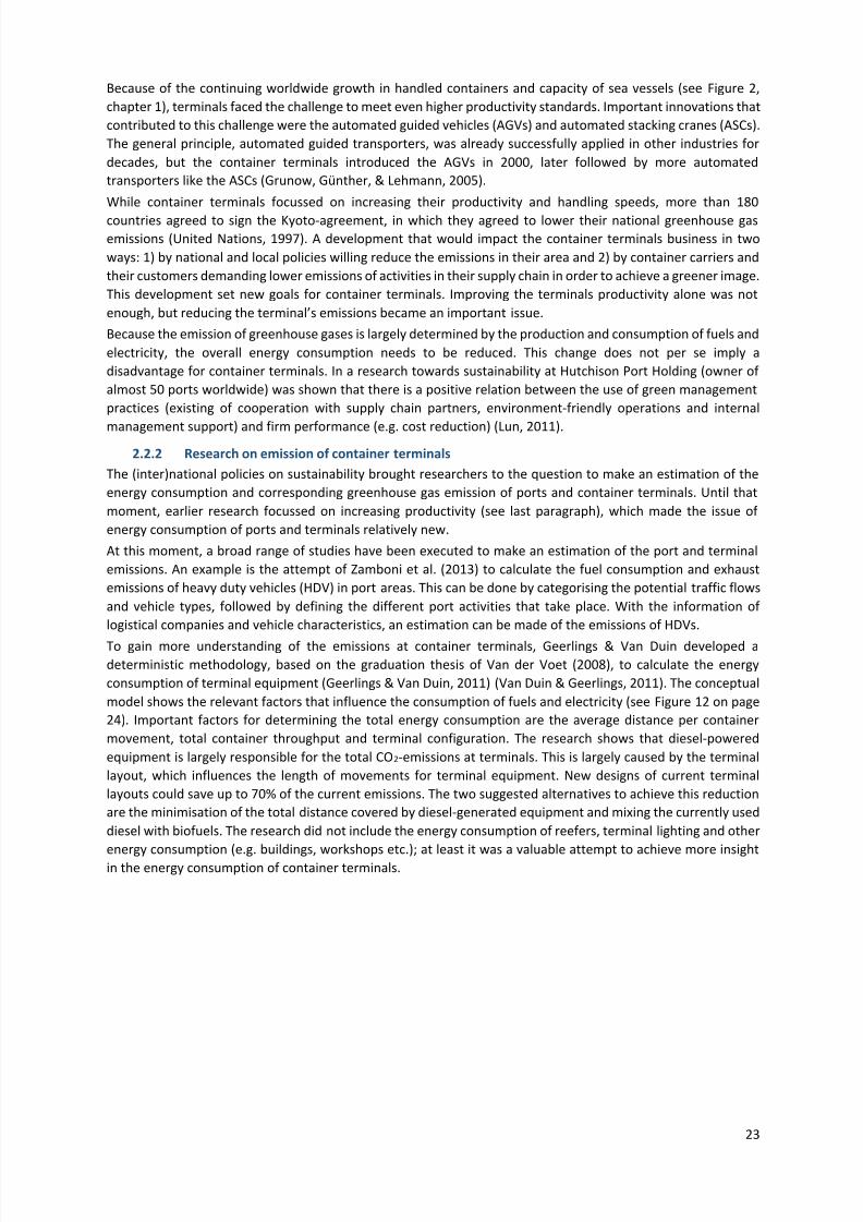
7/23/2019 Thesis Robert Heij Final Digital Version
http://slidepdf.com/reader/full/thesis-robert-heij-final-digital-version 23/94
23
Because of the continuing worldwide growth in handled containers and capacity of sea vessels (see Figure 2,
chapter 1), terminals faced the challenge to meet even higher productivity standards. Important innovations that
contributed to this challenge were the automated guided vehicles (AGVs) and automated stacking cranes (ASCs).
The general principle, automated guided transporters, was already successfully applied in other industries for
decades, but the container terminals introduced the AGVs in 2000, later followed by more automated
transporters like the ASCs (Grunow, Günther, & Lehmann, 2005).
While container terminals focussed on increasing their productivity and handling speeds, more than 180
countries agreed to sign the Kyoto-agreement, in which they agreed to lower their national greenhouse gas
emissions (United Nations, 1997). A development that would impact the container terminals business in two
ways: 1) by national and local policies willing reduce the emissions in their area and 2) by container carriers and
their customers demanding lower emissions of activities in their supply chain in order to achieve a greener image.
This development set new goals for container terminals. Improving the terminals productivity alone was not
enough, but reducing the terminal’s emissions became an important issue.
Because the emission of greenhouse gases is largely determined by the production and consumption of fuels and
electricity, the overall energy consumption needs to be reduced. This change does not per se imply a
disadvantage for container terminals. In a research towards sustainability at Hutchison Port Holding (owner of
almost 50 ports worldwide) was shown that there is a positive relation between the use of green management
practices (existing of cooperation with supply chain partners, environment-friendly operations and internal
management support) and firm performance (e.g. cost reduction) (Lun, 2011).
2.2.2
Research on emission of container terminals
The (inter)national policies on sustainability brought researchers to the question to make an estimation of the
energy consumption and corresponding greenhouse gas emission of ports and container terminals. Until that
moment, earlier research focussed on increasing productivity (see last paragraph), which made the issue of
energy consumption of ports and terminals relatively new.
At this moment, a broad range of studies have been executed to make an estimation of the port and terminal
emissions. An example is the attempt of Zamboni et al. (2013) to calculate the fuel consumption and exhaust
emissions of heavy duty vehicles (HDV) in port areas. This can be done by categorising the potential traffic flows
and vehicle types, followed by defining the different port activities that take place. With the information of
logistical companies and vehicle characteristics, an estimation can be made of the emissions of HDVs.
To gain more understanding of the emissions at container terminals, Geerlings & Van Duin developed a
deterministic methodology, based on the graduation thesis of Van der Voet (2008), to calculate the energy
consumption of terminal equipment (Geerlings & Van Duin, 2011) (Van Duin & Geerlings, 2011). The conceptual
model shows the relevant factors that influence the consumption of fuels and electricity (see Figure 12 on page
24). Important factors for determining the total energy consumption are the average distance per container
movement, total container throughput and terminal configuration. The research shows that diesel-powered
equipment is largely responsible for the total CO2-emissions at terminals. This is largely caused by the terminal
layout, which influences the length of movements for terminal equipment. New designs of current terminal
layouts could save up to 70% of the current emissions. The two suggested alternatives to achieve this reduction
are the minimisation of the total distance covered by diesel-generated equipment and mixing the currently used
diesel with biofuels. The research did not include the energy consumption of reefers, terminal lighting and other
energy consumption (e.g. buildings, workshops etc.); at least it was a valuable attempt to achieve more insight
in the energy consumption of container terminals.
7/23/2019 Thesis Robert Heij Final Digital Version
http://slidepdf.com/reader/full/thesis-robert-heij-final-digital-version 24/94
24
Figure 12: Conceptual model for determining energy consumption of terminal equipment
Source: (Van der Voet, 2008) (Van Duin & Geerlings, 2011)
In further research an attempt was made to gain more understanding of the energy consumption of the other
processes, like for example the reefers. A first exploratory study to estimate the energy consumption and
corresponding CO2-emission of reefers at the Port of Rotterdam showed an annual electricity consumption of
80-189 million kWh, equal to a CO2-emission between 49.9 and 117.9 kilotons (Heij, 2012). Converted to the
emission per container, this is between 4,158 and 9,825 kg. CO 2 per reefer per year (with reefers having an
average stay of 5.3 days). Where the total energy consumption of all container terminals was estimated at 140
kiloton CO2 (Geerlings & Van Duin, 2011), reefers would be responsible for 35% - 80% of the total energy
consumption.
Based on the energy consumption of the Noatum Container Terminal in Valencia (NCTV) during 2011 and 2012,
the electricity consumption of container terminals was calculated (GreenCranes, 2013). The consumption of
reefers is estimated at approximately 45%, crane movements at 35%, energy consumption of buildings at 15%
and finally the yard lightning at 5% (see Figure 13). The other terminal processes (e.g. terminal trucks, rubber-tired gantry’s and straddle carriers) are powered with (bio)diesel and are therefore not included in this graph.
Figure 13: Overview of electricity usage at Noatum Container Terminal in Valencia
Source: (GreenCranes, 2013)
The referred studies in this paragraph are a first estimation of the energy consumption at container terminals
and mark the beginning of a process towards a better academic understanding. Although terminal operators
know the energy consumption of their terminal in detail, they are reluctant to share this information as they fear
competitive disadvantages. The academic researchers are therefore still dependent on deterministic
calculations. It might be expected that the accuracy and scope of academic research will increase and estimations
will come close towards the exact energy consumption.
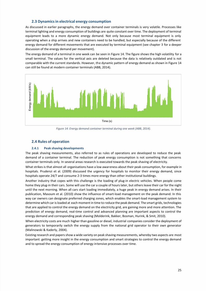
7/23/2019 Thesis Robert Heij Final Digital Version
http://slidepdf.com/reader/full/thesis-robert-heij-final-digital-version 25/94
25
2.3 Dynamics in electrical energy consumption
As discussed in earlier paragraphs, the energy demand over container terminals is very volatile. Processes like
terminal lighting and energy consumption of buildings are quite constant over time. The deployment of terminal
equipment leads to a more dynamic energy demand. Not only because most terminal equipment is only
operating when a ship arrives and new containers need to be handled, but especially because of the different
energy demand for different movements that are executed by terminal equipment (see chapter 3 for a deeper
discussion of the energy demand per movement).
The energy demand of a terminal in one week can be seen in Figure 14. The figure shows the high volatility for a
small terminal. The values for the vertical axis are deleted because the data is relatively outdated and is not
comparable with the current standards. However, the dynamic pattern of energy demand as shown in Figure 14
can still be found at modern container terminals (ABB, 2014).
Figure 14: Energy demand container terminal during one week (ABB, 2014).
2.4 Rules of operation
2.4.1 Peak shaving developments
The peak shaving measurements, also referred to as rules of operations are developed to reduce the peakdemand of a container terminal. The reduction of peak energy consumption is not something that concerns
container terminals only. In several areas research is executed towards the peak shaving of electricity.
What strikes is that almost all organisations have a low awareness about their peak consumption, for example in
hospitals. Prudenzi et al. (2009) discussed the urgency for hospitals to monitor their energy demand, since
hospitals operate 24/7 and consume 2-3 times more energy than other institutional buildings.
Another industry that copes with this challenge is the loading of plug-in electric vehicles. When people come
home they plug-in their cars. Some will use the car a couple of hours later, but others leave their car for the night
until the next morning. When all cars start loading immediately, a huge peak in energy demand arises. In their
publication, Masoum et al. (2010) show the influence of smart-load management on the peak demand. In this
way car owners can designate preferred charging zones, which enables the smart-load management system to
determine which car is loaded at each moment in time to reduce the peak demand. The smart grids, technologiesthat are applied to control the energy demand on the electricity grid, are gaining more and more attention. The
prediction of energy demand, real-time control and advanced planning are important aspects to control the
energy demand and corresponding peak shaving (Molderink, Bakker, Bosman, Hurink, & Smit, 2010).
When electricity costs are much higher than gasoline or diesel, industrial companies consider the deployment of
generators to temporarily switch the energy supply from the national grid operator to their own generator
(Malinowski & Kaderly, 2004).
Existing research and papers show a wide variety on peak shaving measurements, whereby two aspects are most
important: getting more insight in the energy consumption and smart strategies to control the energy demand
and to spread the energy consumption of energy intensive processes over time.
E n e r g y d e m a n d ( k W / s )
Time (s)
7/23/2019 Thesis Robert Heij Final Digital Version
http://slidepdf.com/reader/full/thesis-robert-heij-final-digital-version 26/94
26
2.4.2 Peak shaving measurements for container terminals
The rules of operation can be seen as measures that can be taken by container terminals to influence the peak
demand of their container terminals. As concluded in last sub-paragraph, first more insight is needed in the
energy consumption. Next to that, the implementation of a smart management system enables a company to
reduce their peak demand. This system should contain strategies to spread the energy consumption over time
(peak shaving).
As such, the developed consumption and simulation model in this research (see chapter 3) can be used to gain
more insight in the energy consumption, where the application of rules of operation can be seen as smart
management system.
In the simulation model two rules of operation are implemented:
1. Limitation of the number of quay cranes lifting at the same moment
The first rule of operation, the restriction of the number of simultaneously lifting quay cranes, looks at
what happens when not all operational quay cranes are enabled to lift containers at the same moment.
A quay crane has two lifting ‘movements’ (see paragraph 3.4): the lifting of the spreader and container
above the ship and the lifting of the (empty) spreader above the quay). When for example maximum
four of the eight quay cranes is enable to lift at the same moment, no more than four quay cranes are
enabled to process a container through one of the two lifting movements.
2. Limitation of maximum energy demand per secondThe second rule of operation deals with the maximum energy demand. This can be set at a certain kW-
demand, to impose a maximum for all quay cranes. Before starting a new movement, every quay crane
requests the energy that it is expecting to use (dependent on the movement and the container load).
Based on this expected demand, the model looks whether this demand is available. If not, the quay
crane is asked to pause, until there is enough demand left to start the movement. When quay cranes
are asked to pause, they are queued in a first-in-first-out principle, which means that the quay crane
that is waiting the longest, will be the first to get clearance to restart operations. It is assumed that quay
cranes can only pause in between the six general movements. In the simulation model all general
movements are divided into two or three sub-movements. However, stopping in between the sub-
movements would costs so much energy, that the general principle behind this rule of operations would
be undone.
The rules of operation are implemented in the simulation model to enable the experiments. The rules of
operation are executed for two types of container terminals: a terminal with 6 operational quay cranes and a
terminal with 8 operational quay cranes. This enables the comparison of the impact of the rules of operation for
different container terminals.
The two rules of operation are tested to investigate their impact on the peak demand and handling time. As such,
a rule of operation can be seen as (part of) a smart management system (see paragraph 2.4.1) to control the
energy demand. Chapter 4 discusses the different results of these analyses. The results for each rule of operation
will be compared with the current situation on two criteria:
- influence on the height of the electrical peak demand (in kW);
- influence on the average handling time.
2.5 Knowledge gap
Derived from the first paragraphs of this chapter, the knowledge gap deals with the dynamic visualisation of the
energy consumption at container terminals. Based on the existing challenge to reduce the energy emissions,
earlier research used a more deterministic approach to visualise the total energy consumption over time (in
kWh/year or L/year). This resulted in several studies which, based on general assumptions, describe the energy
consumption of separate terminal processes. However, there are three lacking elements in the existing
approaches that form the knowledge gap:
1. Existing energy consumption models are not developed to visualise the energy consumption per second,
which is needed to dynamically visualise the energy demand over time (in kW/s). A model that is able
to do this is therefore developed in this research.
2. The container terminal business is faced with growing uncertainty (e.g. high competition, energy price
uncertainty and geopolitical tensions) forcing them to make their operations more efficient, mainly
achieved by cost reduction. To be able to reduce the energy related costs, first more insight is needed

7/23/2019 Thesis Robert Heij Final Digital Version
http://slidepdf.com/reader/full/thesis-robert-heij-final-digital-version 27/94
27
in the energy consuming processes and opportunities that might contribute to a reduction. This research
presents opportunities for reducing the peak-related energy costs of terminal equipment.
3. Grid operators calculate the electricity price for container terminals partly based on the peak energy
consumption of terminals. The higher the observed peak, the higher the costs. The challenge for
container terminals is therefore to smoothen their energy consumption over time to prevent high peaks
in energy demand. However, it is unknown to what extent the peak demand can be reduced. This
research presents to which extent this peak demand can be reduced.
Derived from these three missing aspects, the knowledge gap is how to develop a more detailed representation
of container terminal processes that shows the dynamic energy demand of electricity over time in order to test
the impact of different process innovations and possibilities for peak shaving of this energy demand.
2.6 Conclusion
The literature review in this chapter has analysed earlier executed research and showed the important processes
which are responsible for a terminal’s energy consumption. Earlier research (sub-question 1) has shown that the
ongoing innovations towards terminal equipment led to more efficient container terminal processes and the use
of cleaner energy sources like hybrid systems and electricity instead of diesel. However, the terminal layout is
also highly responsible for the energy consumption and new layouts could save up to 70%. The earlier research
is based on deterministic approaches with a focus on the annual energy consumption in kWh/year. There is no
existing study known that represents the dynamic energy demand of complete container terminals in kW/s.
The processes that determine the energy consumption of container terminals (sub-question 2) can be divided
into transportation processes and other processes. The transportation processes are the (un)loading of
containers between ship and shore, transport of containers between quay side and stacks, the stacking of
containers, inter-terminal transport between stacks and trains/trucks and finally the equipment used for
(un)loading the trains and trucks. The other processes are the energy consumption of reefers, terminal lighting
and buildings (e.g. workshops, offices, freight stations etc.).
Because existing studies do not visualise the energy consumption of a container terminal in kW/s, the peak
demand cannot be visualised before developing an energy consumption model and subsequently a simulation
model to visualise the energy demand over time and to analyse the peak demand. This chapter has presented all
relevant processes that need to be taken into account for determining the energy demand of a container
terminal, which forms the basis for the calculation model in the next chapter.

7/23/2019 Thesis Robert Heij Final Digital Version
http://slidepdf.com/reader/full/thesis-robert-heij-final-digital-version 28/94
28
View on the Port of Rotterdam in morning light
Photo: Cees van der Wal (twitter.com/vdWalfotografie, 5 March 2014)
3. Energy consumption model
Chapter 2 showed that the energy demand at a container terminal is very volatile and dependent on peak
productivity of terminal equipment. Existing studies towards energy consumption at container terminals mainly
focused on the overall energy consumption. Because of the high costs of peaks in energy demand, it is necessaryto develop a consumption model that shows the dynamics over time. This chapter presents an energy
consumption model which is able to visualise this energy demand (kW/s) over time. Subsequently a simulation
study is developed to identify the peak demand for an existing container terminal and to test to what extent the
developed rules of operation contribute to a reduction in peak demand.
Paragraph 3.1 focuses on the development of a consumption model that takes into account all relevant aspects
of electrical-powered terminal processes dealing with a dynamic energy demand over time. Processes with a
steady energy demand (e.g. terminal lighting and buildings) will not be taken into account. Derived from this
consumption model, an overview of required data is presented in paragraph 3.2. Based on the consumption
model and required data a simulation model is applied for a case-study terminal in Valencia. The model
development is described in paragraph 3.3, followed by a description of the model design in paragraph 3.4. After
the model is validated in paragraph 3.5, the chapter is concluded in paragraph 3.6.
3.1 Development of consumption model
By developing the consumption model, it is important to identify all container terminal processes (see paragraph
2.1). Based on this overview an analysis can be made of all electricity-powered terminal processes. However, a
distinction needs to be made between processes with a volatile energy demand and a steady energy demand.
The steady processes do not have any influence on the occurrence of peaks, which is important to answer the
main question of this research (see chapter 1.4). Therefore the steady processes are disregarded from now on.
The energy consumption of reefers, which is influencing the peak demand because of its variable consumption
over time, is also not included. The reason for this is that adding the reefer energy consumption would make this
research too comprehensive.
Regarding the part of the terminal equipment consumption, the consumption model is partly based on the work
of Van der Voet, who tried to create a deterministic insight in the energy consumption and carbon dioxide
emissions of terminal equipment (Van der Voet, 2008). Van der Voets research was based on average distances
on terminals and the average energy consumption per move, which was a valuable first attempt to create insight
in the energy consumption of particular terminal processes and for specific terminal equipment.
In order to gain more understanding of the different terminal processes and energy consuming elements of these
processes, the IDEF0 (Integrated DEFiniton) method is used to construct process schemes. This method will be
explained in paragraph 3.1.1.
3.1.1 IDEF0
The IDEF0-schemes are part of the IDEF modelling language which is often used in systems engineering. The
IDEF0 method represents the functions and its ICOMs: Inputs, Controls, Outputs and Mechanisms (Sage &
Armstrong, 2000). As shown in Figure 15, on the left side of the scheme, an input enters the function/processbox. The controls that are needed for the process (e.g. data) enter on the top side of the box. The mechanisms

7/23/2019 Thesis Robert Heij Final Digital Version
http://slidepdf.com/reader/full/thesis-robert-heij-final-digital-version 29/94
29
(entering from below) show the means needed for executing the process (e.g. machines or operators), which is
of interest because these mechanisms are responsible for the energy consumption of the corresponding process.
When the process is ‘executed’, outputs are leaving at the right side.
A0
Function / ProcessInput Output
Mechanism
Control
Figure 15: IDEF0 process scheme
The IDEF0-method enables construction of models with a top-down representation, but which are built on
bottom-up processes. This is done via decompositions of general processes. Although the IDEF0-method was not
developed to represent the sequence of activities, the method can easily be used to do so (IDEF, 2014).
The highest representation of all container terminals is shown in the A0 scheme (see Figure 16). Here the general
process of the container handling is visualized with all required controls and mechanisms. The controls mainly
refer to data requirements or activation signals, where the mechanisms often show the needed terminal
equipment and its operators.
The containerships, trains and trucks enter the container terminal, often loaded with containers. With the help
of terminal equipment (visualised below the A0-box), the containers are handled according to the plans that are
developed by the Terminal Operating System (TOS). After handling all arrived containers, the containerships,
trucks and trains leave the terminal. Because energy is used for all terminal processes, emissions are a result of
this energy consumption and can be regarded as output of the handling process.
A0
Handling of
containers
Containerships
Trains
Trucks
Containers
Containerships
Trains
Trucks
Containers
Emissions
Energy (electricity/diesel)
Captain containership
Quay cranes
Stacking cranes
Crane operators
Terminal transporters
Transporter operators
Rail crane
(Crane operator)
Terminal transporter
Truck driver
Terminal layout
Arrival scheme
Berthing procedure
Vessel specifications
Terminal specifications
Container specifications
Handling plan
Stacking plan
Unstacking plan
Loading plan truck/train
Figure 16: A0 scheme of container terminal
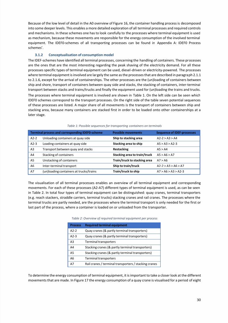
7/23/2019 Thesis Robert Heij Final Digital Version
http://slidepdf.com/reader/full/thesis-robert-heij-final-digital-version 30/94
30
Because of the low level of detail in the A0 overview of Figure 16, the container handling process is decomposed
into some deeper levels. This enables a more detailed exploration of all terminal processes and required controls
and mechanisms. In these schemes one has to look carefully to the processes where terminal equipment is used
as mechanism, because these movements are responsible for the energy consumption of the involved terminal
equipment. The IDEF0-schemes of all transporting processes can be found in Appendix A: IDEF0 Process
schemes’.
3.1.2
Conceptualisation of consumption modelThe IDEF-schemes have identified all terminal processes, concerning the handling of containers. These processes
are the ones that are the most interesting regarding the peak shaving of the electricity demand. For all these
processes specific types of terminal equipment can be used, diesel-driven or electricity-powered. The processes
where terminal equipment is involved are largely the same as the processes that are described in paragraph 2.1.1
to 2.1.6, except for the arrival of containerships. The other processes are the (un)loading of containers between
ship and shore, transport of containers between quay side and stacks, the stacking of containers, inter-terminal
transport between stacks and trains/trucks and finally the equipment used for (un)loading the trains and trucks.
The processes where terminal equipment is involved are shown in Table 1. On the left side can be seen which
IDEF0 schemes correspond to the transport processes. On the right side of the table seven potential sequences
of these processes are listed. A major share of all movements is the transport of containers between ship and
stacking area, because many containers are stacked first in order to be loaded onto other containerships at a
later stage.
Table 1: Possible sequences for transporting containers on terminals
Terminal process and corresponding IDEF0-scheme Possible movements Sequence of IDEF-processes
A2-2 Unloading containers at quay side Ship to stacking area A2-2 > A3 > A4
A2-3 Loading containers at quay side Stacking area to ship A5 > A3 > A2-3
A3 Transport between quay and stacks Restacking A5 > A4
A4 Stacking of containers Stacking area to train/truck A5 > A6 > A7
A5 Unstacking of containers Train/truck to stacking area A7 > A6
A6 Inter-terminal transport Ship to train/truck A2-2 > A3 > A6 > A7
A7 (un)loading containers at trucks/trains Train/truck to ship A7 > A6 > A3 > A2-3
The visualisation of all terminal processes enables an overview of all terminal equipment and corresponding
movements. For each of these processes (A2-A7) different types of terminal equipment is used, as can be seen
in Table 2. In total four types of terminal equipment can be distinguished: quay cranes, terminal transporters
(e.g. reach stackers, straddle carriers, terminal trucks) stacking cranes and rail cranes. The processes where the
terminal trucks are partly needed, are the processes where the terminal transport is only needed for the first or
last part of the process, where a container is loaded on or unloaded from the transporter.
Table 2: Overview of required terminal equipment per process
Process Required terminal equipmentA2-2 Quay cranes (& partly terminal transporters)
A2-3 Quay cranes (& partly terminal transporters)
A3 Terminal transporters
A4 Stacking cranes (& partly terminal transporters)
A5 Stacking cranes (& partly terminal transporters)
A6 Terminal transporters
A7 Rail cranes / terminal transporters / stacking cranes
To determine the energy consumption of terminal equipment, it is important to take a closer look at the different
movements that are made. In Figure 17 the energy consumption of a quay crane is visualised for a period of eight
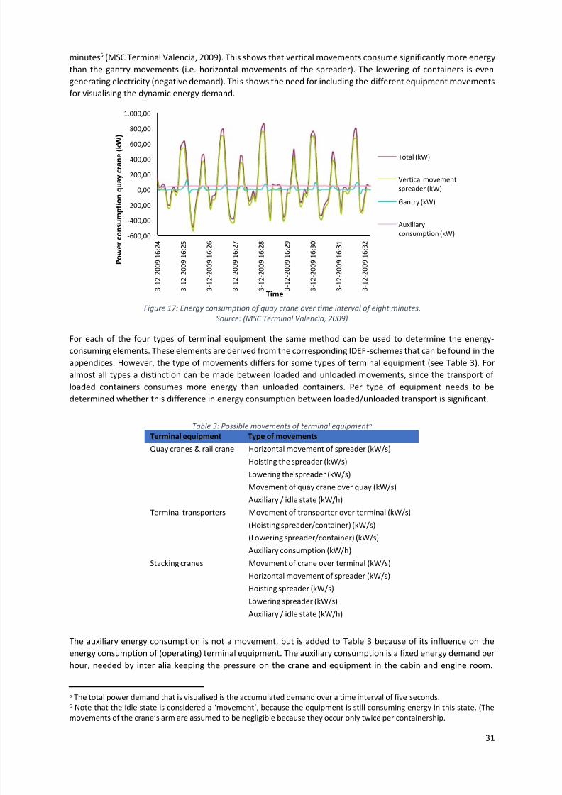
7/23/2019 Thesis Robert Heij Final Digital Version
http://slidepdf.com/reader/full/thesis-robert-heij-final-digital-version 31/94
31
minutes5 (MSC Terminal Valencia, 2009). This shows that vertical movements consume significantly more energy
than the gantry movements (i.e. horizontal movements of the spreader). The lowering of containers is even
generating electricity (negative demand). This shows the need for including the different equipment movements
for visualising the dynamic energy demand.
Figure 17: Energy consumption of quay crane over time interval of eight minutes.
Source: (MSC Terminal Valencia, 2009)
For each of the four types of terminal equipment the same method can be used to determine the energy-
consuming elements. These elements are derived from the corresponding IDEF-schemes that can be found in the
appendices. However, the type of movements differs for some types of terminal equipment (see Table 3). For
almost all types a distinction can be made between loaded and unloaded movements, since the transport of
loaded containers consumes more energy than unloaded containers. Per type of equipment needs to be
determined whether this difference in energy consumption between loaded/unloaded transport is significant.
Table 3: Possible movements of terminal equipment 6
Terminal equipment Type of movements
Quay cranes & rail crane Horizontal movement of spreader (kW/s)
Hoisting the spreader (kW/s)
Lowering the spreader (kW/s)
Movement of quay crane over quay (kW/s)
Auxiliary / idle state (kW/h)
Terminal transporters Movement of transporter over terminal (kW/s)
(Hoisting spreader/container) (kW/s)
(Lowering spreader/container) (kW/s)
Auxiliary consumption (kW/h)
Stacking cranes Movement of crane over terminal (kW/s)
Horizontal movement of spreader (kW/s)
Hoisting spreader (kW/s)
Lowering spreader (kW/s)
Auxiliary / idle state (kW/h)
The auxiliary energy consumption is not a movement, but is added to Table 3 because of its influence on the
energy consumption of (operating) terminal equipment. The auxiliary consumption is a fixed energy demand per
hour, needed by inter alia keeping the pressure on the crane and equipment in the cabin and engine room.
5 The total power demand that is visualised is the accumulated demand over a time interval of five seconds.6 Note that the idle state is considered a ‘movement’, because the equipment is still consuming energy in this state. (The
movements of the crane’s arm are assumed to be negligible because they occur only twice per containership.
-600,00
-400,00
-200,00
0,00
200,00
400,00
600,00
800,00
1.000,00
3 - 1 2 - 2 0 0 9 1 6 : 2 4
3 - 1 2 - 2 0 0 9 1 6 : 2 5
3 - 1 2 - 2 0 0 9 1 6 : 2 6
3 - 1 2 - 2 0 0 9 1 6 : 2 7
3 - 1 2 - 2 0 0 9 1 6 : 2 8
3 - 1 2 - 2 0 0 9 1 6 : 2 9
3 - 1 2 - 2 0 0 9 1 6 : 3 0
3 - 1 2 - 2 0 0 9 1 6 : 3 1
3 - 1 2 - 2 0 0 9 1 6 : 3 2
P o w e r c o n s u m p t i o n q u a y c r a n e ( k W
)
Time
Total (kW)
Vertical movement
spreader (kW)
Gantry (kW)
Auxiliary
consumption (kW)

7/23/2019 Thesis Robert Heij Final Digital Version
http://slidepdf.com/reader/full/thesis-robert-heij-final-digital-version 32/94
32
Together the auxiliary consumption could count up to 140 kW (ABB, 2014). The auxiliary consumption is rather
constant over time because the quay cranes are not turned off while in idle or off-shift state. This means that
even the idle state is important to include in the consumption model. The terminal transporters are an exception,
because they can be switched off completely (ABB, 2014).
By multiplying each of these types of movement with the distance for that movement, the total distance can be
calculated, leading to a certain transport time for that movement. When the starting time of the movement is
known, the energy consumption can be calculated by adding the energy consumption for that particular
movement and the auxiliary energy consumption for that type of equipment. When doing this every second for
all movements for all terminal equipment, the energy consumption will be visualised over time (in kW/s). This is
shown in Figure 18.
DIstance of movement
(m/move)
Total transport time for
particular movement
(s)
Type of movement
(1/move)
Total distance for particular
movement
(m/move)
Energy consumption for
particular movement
(kW/s)
Current energy
consumption equipment
(kW/s)
Auxiliary energy
consumption
(kW/s)
Figure 18: Conceptualisation for determining energy consumption over time interval of movement
Figure 18 shows the energy consumption for a particular movement of a particular type of equipment (since thetype of movements differ for each type of equipment, as explained in above) over the time interval for that
particular movement. For determining the energy consumption per second (kW/s), some adaptions need to be
made to this conceptualisation.
Instead of calculating the distance to be covered, one only needs to know whether the movement is executed or
not. In case the movement is executed, the corresponding energy consumption for that movement can be added
up to the current energy consumption of the terminal. However, the energy consumption for a particular
movement depends on the load of the container (the higher the load, the higher the energy consumption)7. The
new visualisation is presented in Figure 19 (see next page). In paragraph 3.1.3 this visualisation is converted into
the final consumption model.
7 Although it is likely to assume, the energy consumption for a particular movement does not depend on the speed of the
equipment, since the consumption of terminal equipment is proven stable over different speeds (ABB, 2013).
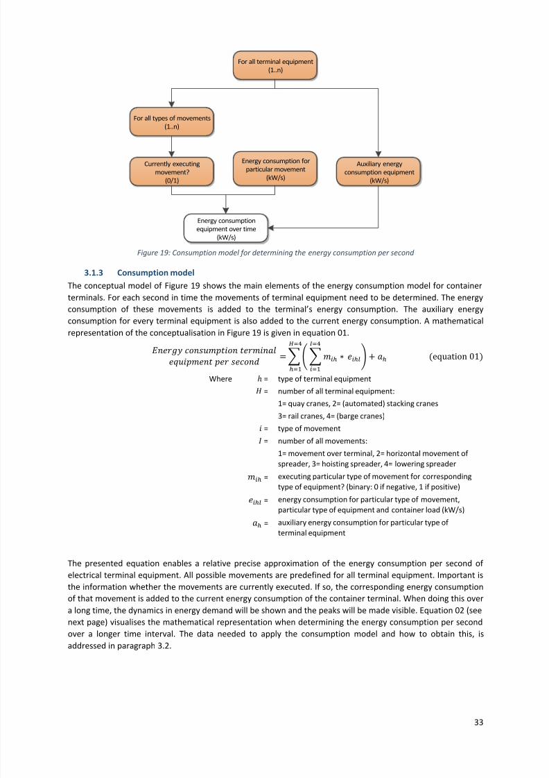
7/23/2019 Thesis Robert Heij Final Digital Version
http://slidepdf.com/reader/full/thesis-robert-heij-final-digital-version 33/94
33
For all types of movements
(1..n)
Energy consumption for
particular movement
(kW/s)
Energy consumption
equipment over time
(kW/s)
Auxiliary energy
consumption equipment
(kW/s)
For all terminal equipment
(1..n)
Currently executing
movement?
(0/1)
Figure 19: Consumption model for determining the energy consumption per second
3.1.3
Consumption modelThe conceptual model of Figure 19 shows the main elements of the energy consumption model for container
terminals. For each second in time the movements of terminal equipment need to be determined. The energy
consumption of these movements is added to the terminal’s energy consumption. The auxiliary energy
consumption for every terminal equipment is also added to the current energy consumption. A mathematical
representation of the conceptualisation in Figure 19 is given in equation 01.
∑ ( ∑ ∗=
=) +
=
= equation 01
Where ℎ = type of terminal equipment = number of all terminal equipment:
1= quay cranes, 2= (automated) stacking cranes
3= rail cranes, 4= (barge cranes)
= type of movement
= number of all movements:
1= movement over terminal, 2= horizontal movement of
spreader, 3= hoisting spreader, 4= lowering spreader = executing particular type of movement for corresponding
type of equipment? (binary: 0 if negative, 1 if positive) = energy consumption for particular type of movement,
particular type of equipment and container load (kW/s) = auxiliary energy consumption for particular type of
terminal equipment
The presented equation enables a relative precise approximation of the energy consumption per second of
electrical terminal equipment. All possible movements are predefined for all terminal equipment. Important is
the information whether the movements are currently executed. If so, the corresponding energy consumption
of that movement is added to the current energy consumption of the container terminal. When doing this over
a long time, the dynamics in energy demand will be shown and the peaks will be made visible. Equation 02 (see
next page) visualises the mathematical representation when determining the energy consumption per second
over a longer time interval. The data needed to apply the consumption model and how to obtain this, is
addressed in paragraph 3.2.
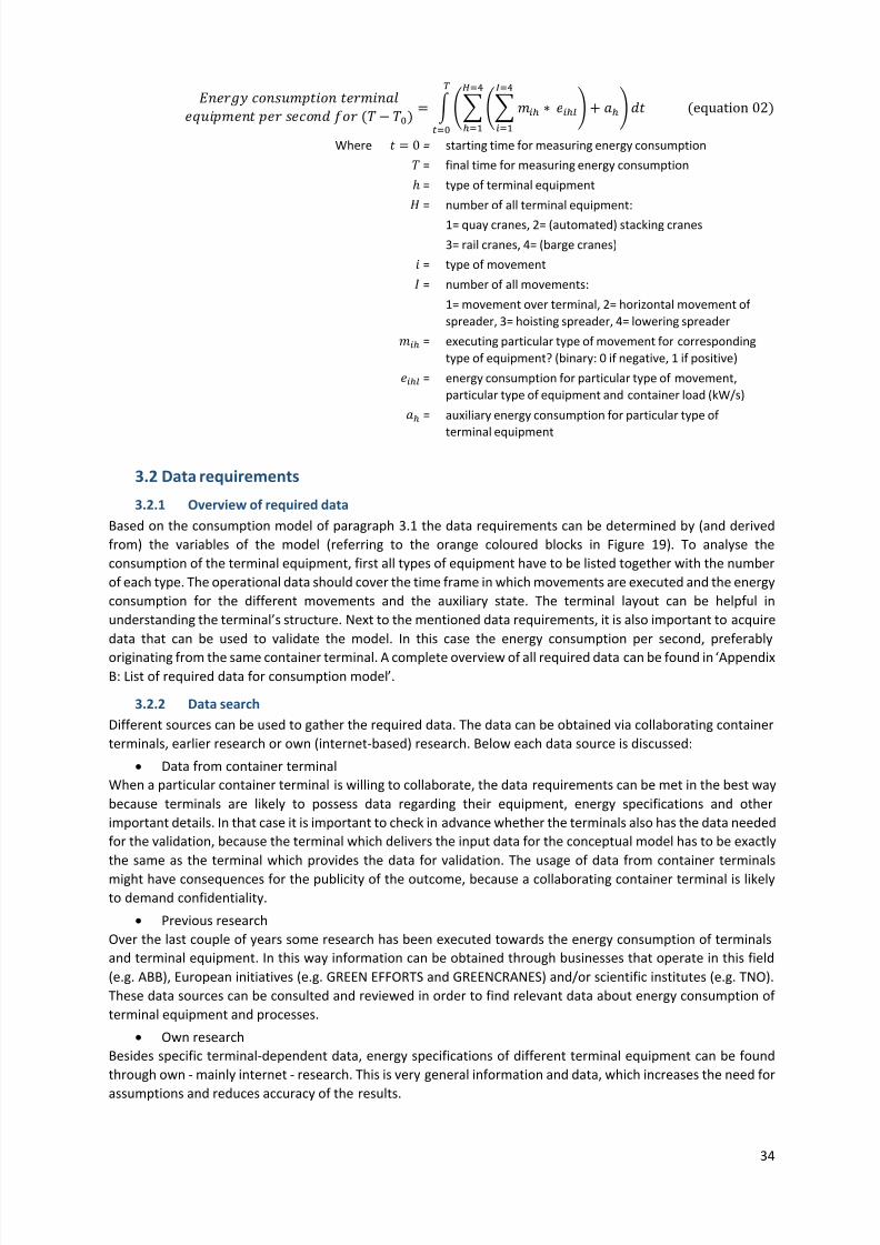
7/23/2019 Thesis Robert Heij Final Digital Version
http://slidepdf.com/reader/full/thesis-robert-heij-final-digital-version 34/94
34
− ∫ (∑ (∑ ∗=
=) +
=
=)
= equation 02
Where 0 = starting time for measuring energy consumption
= final time for measuring energy consumption
ℎ = type of terminal equipment
= number of all terminal equipment:
1= quay cranes, 2= (automated) stacking cranes
3= rail cranes, 4= (barge cranes)
= type of movement
= number of all movements:
1= movement over terminal, 2= horizontal movement of
spreader, 3= hoisting spreader, 4= lowering spreader
= executing particular type of movement for corresponding
type of equipment? (binary: 0 if negative, 1 if positive)
= energy consumption for particular type of movement,
particular type of equipment and container load (kW/s)
= auxiliary energy consumption for particular type of
terminal equipment
3.2 Data requirements
3.2.1
Overview of required data
Based on the consumption model of paragraph 3.1 the data requirements can be determined by (and derived
from) the variables of the model (referring to the orange coloured blocks in Figure 19). To analyse the
consumption of the terminal equipment, first all types of equipment have to be listed together with the number
of each type. The operational data should cover the time frame in which movements are executed and the energy
consumption for the different movements and the auxiliary state. The terminal layout can be helpful in
understanding the terminal’s structure. Next to the mentioned data requirements, it is also important to acquire
data that can be used to validate the model. In this case the energy consumption per second, preferably
originating from the same container terminal. A complete overview of all required data can be found in ‘AppendixB: List of required data for consumption model’.
3.2.2 Data search
Different sources can be used to gather the required data. The data can be obtained via collaborating container
terminals, earlier research or own (internet-based) research. Below each data source is discussed:
Data from container terminal
When a particular container terminal is willing to collaborate, the data requirements can be met in the best way
because terminals are likely to possess data regarding their equipment, energy specifications and other
important details. In that case it is important to check in advance whether the terminals also has the data needed
for the validation, because the terminal which delivers the input data for the conceptual model has to be exactly
the same as the terminal which provides the data for validation. The usage of data from container terminals
might have consequences for the publicity of the outcome, because a collaborating container terminal is likely
to demand confidentiality.
Previous research
Over the last couple of years some research has been executed towards the energy consumption of terminals
and terminal equipment. In this way information can be obtained through businesses that operate in this field
(e.g. ABB), European initiatives (e.g. GREEN EFFORTS and GREENCRANES) and/or scientific institutes (e.g. TNO).
These data sources can be consulted and reviewed in order to find relevant data about energy consumption of
terminal equipment and processes.
Own research
Besides specific terminal-dependent data, energy specifications of different terminal equipment can be found
through own - mainly internet - research. This is very general information and data, which increases the need for
assumptions and reduces accuracy of the results.

7/23/2019 Thesis Robert Heij Final Digital Version
http://slidepdf.com/reader/full/thesis-robert-heij-final-digital-version 35/94
35
3.3 Development of simulation model
3.3.1
Simulation approach
Modelling is a way to support the problem-solving, especially when experiments cannot be executed easily or
are too costly. Over the last years several studies have studied the modelling of (parts of) the processes of
container terminals. Where two elements of the research (i.e. representing all energy consuming terminal
processes and enabling the testing of alternative designs for terminal processes) can be modelled in various ways
(e.g. spreadsheet based programs or simulation tools), the dynamic representation of the energy demand overtime point towards the use of a simulation model. This kinds of models can be used to represent the energy
consumption over time. This paragraph describes several suitable modelling approaches and their application in
academic practice. At the end of the paragraph a choice is made for the most suitable approach.
The existing approaches for modelling container terminals can be categorised as programming-based and
mathematics-based, whereby the programming-based studies can be categorised as agent-oriented or object-
oriented (Xin, Negenborn, & Lodewijks, 2013).
In this paragraph three modelling approaches will be explained in more detail: the more programming-based
Agent-based modelling and Discrete-event simulation and the more mathematical based System Dynamics.
These three approaches give a general overview of the approaches that can be applied:
Agent-based Modelling
Agent-based modelling is built on four main assumptions: agents are autonomous, interdependent,follow simple rules and are adaptive and backward-looking. The agent-based models are modelled
bottom-up and able to adapt their behaviour (e.g. probability or frequency distributions) based on their
learning (Macy & Willer, 2002). The agent-based models consist of active and autonomous entities that
make their own decisions. The benefits of agent-based modelling are the capturing of emergent
behaviours, the natural description of systems and flexibility (Bonabeau, 2002).
Discrete-event Simulation
Object-oriented simulations exist of objects that can be described by entities that take over the
descriptive attributes and behaviour of the object, but can also have its own attributes and behaviour
(Joines & Roberts, 1999). To illustrate this: several gantry cranes (e.g. quay cranes or rail-mounted gantry
cranes) adopt the general attributes and behaviour (e.g. lifting function) of the formulated class ‘gantry
crane’, but can also have their own unique attributes and behaviour (e.g. speed and lifting capacity).
The discrete-event simulation is a well-known simulation program that is based on the object-
orientation. In discrete-event simulations the state of the system changes at discrete points in time,
called events. The system will remain in its state until an event occurs that may change the systems state
(Zeigler, 2003).
System Dynamics
Where the earlier mentioned discrete-event and agent-based modelling approaches are based on
discrete time-bases, the system dynamics approach has a continuous time-flow. Compared to the other
two approaches, the system dynamics approach has the highest abstraction and looks to systems at a
macro level (see Figure 20 on next page). A system dynamics model is developed around differential
equations and mathematical relations between variables. The system uses feedback loops which
describe the system behaviour. Entities in the same stock have the same unit and are threatened
equally, which means that there would be no distinction between types of containers within a particular
stock (Borshchev & Filippov, 2004).

7/23/2019 Thesis Robert Heij Final Digital Version
http://slidepdf.com/reader/full/thesis-robert-heij-final-digital-version 36/94
36
Figure 20: Characteristics of different approaches, ordered by abstraction
Source: (Borshchev & Filippov, 2004)
Application of modelling approaches
In Figure 20 the three described modelling languages are represented. The more object-based discrete event
simulation, agent-based simulation and system dynamics approach can be used to model (parts of) container
terminal processes. Caballini & Sacone (2014) have modelled the rail operations at container terminals in both a
discrete-event approach (Caballini, Pasquale, Sacone, & Siri, 2014) and system dynamics approach (Caballini &Sacone, 2014). Cartenì & De Luca modelled a container terminal environment with a discrete-event approach to
simulate the handling activity time duration (Cartenì & De Luca, 2011). Van Asperen et al. (2010) used the discrete
event simulation to model and test several container stacking rules, also known as stacking algorithms. Alessandri
et al. applied the discrete-event simulation in different studies for modelling the container flows within container
terminals, representing the flows as a system of queues (Alessandri, Cervellera, Cuneo, Gaggero, & Soncin, 2008)
(Alessandri, Sacone, & Siri, 2007).
A different (mathematics-based) approach is developed by Xin et al. (2013). In order to include both the discrete-
event dynamics and continuous-time dynamics of terminal equipment they combined a hybrid system and model
predictive control (MPC). The hybrid system is able to combine the discrete-event en continuous time dynamics
and the MPC is able to deal with many variables with constraints and multiple objectives.
Choice of modelling approachThe choice for a modelling approach very much depends on the feasibility to represent the dynamic energy
consumption of terminal processes, while visualising the execution of the process events at container terminal
and enabling the modeller to adjust the model easily for testing different scenarios. The three discussed
approaches have been compared on several characteristics (see Table 4).
The agent-based approach does not satisfy this purpose because the objects are modelled as autonomous agents
which follow the predefined rules to behave themselves in the system and because the agent-based approach
does not facilitate an event-based modelling of the processes. The system dynamics approach cannot fulfil the
stated requirements because the objects are represented in flows and special specifications cannot be assigned
to separate entities. Despite the noncompliance of the agent-based and system dynamics approaches, the
discrete-event approach is a suitable approach to fulfil the requirements due to its event-based character and
ability to appoint attributes per entity.
The conclusion is therefore to use the discrete-event approaches for constructing the simulation model. For this
purpose the Simio simulation software package of Simio LLC is used. Nevertheless one should keep in mind that
different approaches and software packages have been used to model container terminals, each having their
own advantages and disadvantages.
Table 4: Comparison of modelling approaches
Characteristics Modelling approaches
Agent-based Discrete-event System dynamics
Type of objects Active Passive Flows
Behaviour Autonomous Predefined Predefined
Ability to change
attributes per entityYes Yes No
Distinctive benefitShows emergent
behaviourEvent-based
Shows behaviour of large
interdependent systems

7/23/2019 Thesis Robert Heij Final Digital Version
http://slidepdf.com/reader/full/thesis-robert-heij-final-digital-version 37/94
37
3.3.2 MSC Terminal Valencia
The terminal that is used as a case study for applying the energy consumption model is the MSC Terminal in
Valencia (MSCTV). The MSCTV has a surface of 35 ha. and quay length of 774m. Eight super post panama quay
cranes handle an annual throughput of 1.6 million TEU. The MSCTV has a dated terminal configuration and its
terminal operations are largely dependent on terminal equipment which are diesel-powered (e.g. terminal trucks
for on-terminal transport, rubber-tired gantry cranes for the stacking of containers and reach stackers for
(un)loading trains and trucks). The only electrical powered equipment are the eight Super Post Panamax
PORTAINER® quay cranes from Paceco (see Figure 21). These cranes have an outreach up to 65 meter and the
spreader is able to lift a maximum of 65 tonnes gross weight over 41 meter (Paceco España, 2010).
Figure 21: Super post panamax quay cranes at MSC Terminal in Valencia.
Source: MSCTV (2010)
All electrical powered processes (i.e. the eight quay cranes, reefers, terminal lighting and other processes
like buildings and workshops) consume over 12 million kWh (MSC, 2012). In Figure 22 is shown how this
consumption is distributed over the mentioned processes. The quay crane operations are responsible for
50% of the energy consumption of the MSCTV and show a highly volatile demand. This is the reason for
demarcating the simulation model around the operations of the quay cranes.
Figure 22: Distribution of energy consumption (kWh) of MSCTV (2012)
3.3.3
Model specificationsNow the simulation approach and case-study container terminal to apply the consumption model have been
chosen, the simulation model can be constructed. In paragraph 3.1.2 the data requirements for the consumption
model are discussed (see also ‘Appendix B: List of required data for consumption model’). In order to apply the
consumption model in a simulation environment for a real container terminal, the following data have to be
available:
- terminal layout specifications (i.e. number of quay cranes);
- arrival scheme containerships;
- number of containers to be handled;
- container load specifications;
- position of containers;
- energy consumption specifications.
Quay cranes
50%
Reefers
36%
Terminal
lighting
3%
Buildings
11%

7/23/2019 Thesis Robert Heij Final Digital Version
http://slidepdf.com/reader/full/thesis-robert-heij-final-digital-version 38/94
38
The terminal lay-out specifications are needed to understand the setup of the terminal’s quay cranes and the
number of operating quay cranes. Based on the arrival scheme and number of handled containers per
containership the different movements can be simulated. Derived from the containers’ location on the ship and
the speed of the quay crane, the duration for each movement of the quay crane can be determined.
The data for constructing the simulation model is provided by ABB, a professional company active in the field of
electrical engineering and automatisation. The obtained data fulfils the above mentioned requirements. Divided
over the different type of movements and different container loads (varying from 0% for empty containers to
100% for full containers, with intervals of 10%) the energy consumption and duration are known. However, there
is a difference compared to the four types of movements for quay cranes presented in paragraph 3.1.
ABB makes a distinction between the hoisting and lowering of the quay crane above the containership and above
the quay. This means that the total number of movements increases from four to six. Next to this, ABB subdivided
the six movements into 2-3 sub-movements to enable a more detailed visualisation of the energy demand of the
quay cranes. An example is the movement of the spreader from quay to ship. The first part of the movement
consumes energy because the spreader needs to accelerate. However, the second (and last) part of the
movement generates energy because the spreader is slowed down. In this way the peaks can be visualised more
realistically, as is shown in Figure 23. As can be seen, the blue line has higher peaks and lower falls than the
orange line (using an average energy consumption per movement), which shows the extra detail that is obtained
when using sub-movements for visualising the energy demand.
Figure 23: Energy demand for handling a container with and without sub -movements (ABB, 2014)
The simulation model is constructed to measure the peak energy demand (in kW/s) as well as the handling time
for the number of containers that are included in the simulation run. This enables the research of the trade-off
between the reduction of the energy demand and the corresponding consequences for the handling time (see
chapter 1). This is tested for different rules of operation, which will be introduced in chapter 4 in more detail.
Figure 24 gives an overview of all inputs and outputs of the simulation model, as well as the rules of operation
that are tested. The rules of operation will be explained in more detail in chapter 4.
-3.000
-2.000
-1.000
0
1.000
2.000
3.000
4.000
E n e r g y d e m a n d ( k W )
Time for handling container (sec.)
Data with sub-movements
Energy demand without sub-movements

7/23/2019 Thesis Robert Heij Final Digital Version
http://slidepdf.com/reader/full/thesis-robert-heij-final-digital-version 39/94
39
Simulation model
R u l e s o f o p e r a t i o n
- (Current situation)
- Limiting number of hoisting
quay cranes
- Limiting maximum energy
consumption per second
- Peak energy consumption
(kW/s)
- Handling t ime of
containers (seconds)
- Terminal lay-out specifications
- Arrival scheme ships
- Number of handled containers
- Container load specifications
- Position of containers- Energy consumption specifications
Figure 24: Overview of inputs and outputs simulation model
3.3.4
Scope and time span
The scope of the simulation model deals with the operations of the quay cranes, since this is the only electricityconsuming terminal process at MSCTV that experiences a strong volatile demand change over time. For this
purpose the quay crane handling processes are decomposed to give a more detailed understanding of the
operations. In ‘Appendix C: IDEF0 process schemes for (un)loading containers’ the two decompositions for the
processes of unloading and loading containers at the quay side are presented. Based on this extensive process
description (where all possible movement of the quay cranes have been included) and the developed energy
consumption model a simulation model can be developed.
The rules of operation are compared with each other based on a week of operations at the MSCTV (1-7 December
2012). In this time period 19 containerships arrived, ranging from 303 to 3,805 TEU per containership, with an
average of 1,058 TEU per containership. In total, the container terminal handled 20,114 TEU during that week.
Because the simulation model assumes a container handling with 40ft containers only (see paragraph 3.3.5), the
number of containers that arrive in the simulation model is set to 10,057 containers8. The detailed arrival scheme
can be found in ‘Appendix D: Arrival scheme containerships’.
The run length of the simulation period is one week, which is 168 hours. The longest cycle time within the
simulation model is the handling of the largest containership. With an average handling time of 78.0 seconds per
container (ABB, 2014) and eight available quay cranes, the handling of the 3,805 containers would take
approximately 10 hours9. A rule of thumb is that the runtime of the model should be at least three times the
longest cycle time (Kelton, 2000). This precondition is satisfied in the simulation model, since the run time is
sixteen times the longest cycle time. No warm-up period is used, because the arrival times of containerships are
based on a data table (see ‘Appendix D: Arrival scheme containerships’). The number of replications is discussed
in paragraph 3.5.1.
3.3.5 Model assumptions
For constructing the simulation model some assumptions have to be made due to the lack of precise data or to
simplify (sub) processes of some complex terminal operations. The assumptions are divided over three
categories: significant impact, low impact, negligible impact and unknown. Especially the significant assumptions
and assumption with an unknown effect are important because of their potential influence on the results of the
simulation model.
Significant
- The spreader of a quay crane is able to lift one 40ft. container or two 20ft. containers per move. The
spreader always transports 2 TEU per move (i.e. two 20ft. containers or 40 ft. container).
Effect: in reality not all 20 ft. containers are moved in pairs, which means that the average of 2
TEU/move is assumed too high. The number of 20ft. containers is around 50% of all handled containers
8
, TEU TEU/ = 10,057 containers
9 , ∗ ./
y = 10.3 hours
7/23/2019 Thesis Robert Heij Final Digital Version
http://slidepdf.com/reader/full/thesis-robert-heij-final-digital-version 40/94
40
(MSC Terminal Valencia, 2012). If only half of the 20ft. containers are transported in pairs, the average
is around 1.7 TEU/move, which increases the number of moves with 14%. For 25% of the simulated
movements the energy consumption will be less than modelled, because the movement is executed
with only one 20ft. container instead of two. The exact influence on the energy demand is unknown
because the data makes no distinction between moving a 20ft. container and a 40ft. container, but is
considered to be significant. In general can be stated that if the number of moves increases and the
container weight decreases, the peak demand will be lower.
Low
- The data uses average energy consumption specifications for containers, dependent on their load
percentage (100% is full load, 0% is an empty container). The location of the container on the ship is not
included in the provided data, which means that for all container the same location is assumed.
Effect: the effect on the peak in energy demand is not significant, as shown in the sensitivity analysis
(see paragraph 3.4.2). The change in peak demand was proven to be only 0.75%.
- The movements of quay cranes on their track on the land side of the terminal is neglected because there
is no data known about the energy consumption for this type of movement.
Effect: this might affect the outcome in the way that the corresponding energy consumption is not
included in the total energy demand, however the energy demand of this type of movement is
considered low (ABB, 2014).
Negligible- No distinction is made between the incoming containers and outgoing containers, because the available
data does not provide for this.
Effect: the consequence of this assumption is negligible, because the same movements are made for
incoming and outgoing containers. A difference is that some energy specifications will be swapped, e.g.
the highest peak for incoming containers (which is the hoisting above the ship) will be shifted towards
hoisting the container above the quay (in case of outgoing containers).
- There are always trucks available at the quay cranes for containers to be loaded from quay crane onto
the terminal truck. The consequence is that the quay crane processes are not delayed by terminal trucks
that are assigned to pick up containers at a particular quay crane and which do not arrive in time.
Effect: this assumption allows the quay crane to continue its movement directly from horizontal ship to
shore process into the lowering at quay side process, without holding the container to wait for thearriving terminal trucks. The holding of a container would not increase the energy demand (the energy
consumption for holding a container is not higher than for moving a container). The only effect would
be that a quay crane could not continue its operations directly. Because the model is stochastic, it is
expected that this assumption does not affect the energy peak demand.
Unknown
- In the new rules of operation, where either the energy consumption or number of lifting quay cranes is
limited, some containers are queued during their movement from ship to shore (or vice versa), which
means that containers can temporarily be stopped moving between different movements. It is assumed
that quay cranes do not consume energy during these stops.
Effect: in reality some energy will be consumed for holding a container in its place. Unfortunately it is
not known how much influence this assumption has on the model.
3.4 Description of simulation model
After the conceptual model for the simulation has been developed according to the presented characteristics
and assumptions (see paragraph 3.3), the model is constructed. In this paragraph the model is described in
general, followed by the model verification (including sensitivity analysis) and validation (Sargent, 2013).
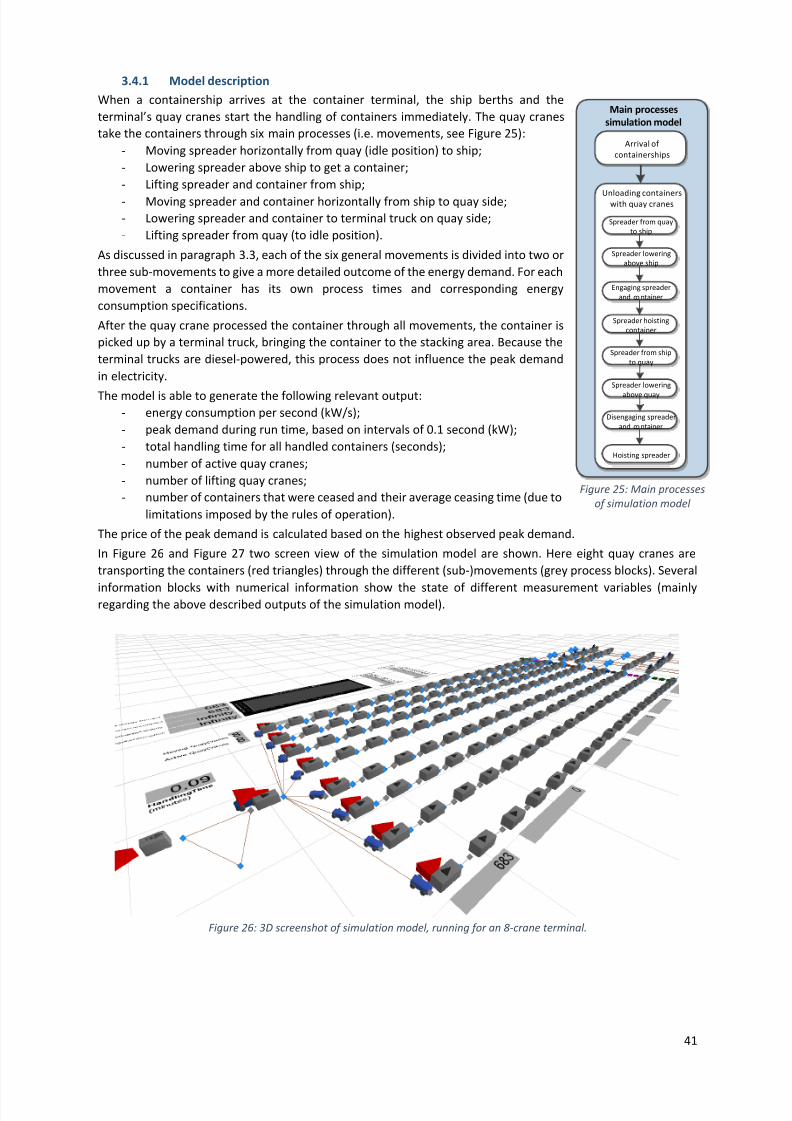
7/23/2019 Thesis Robert Heij Final Digital Version
http://slidepdf.com/reader/full/thesis-robert-heij-final-digital-version 41/94
41
3.4.1 Model description
When a containership arrives at the container terminal, the ship berths and the
terminal’s quay cranes start the handling of containers immediately. The quay cranes
take the containers through six main processes (i.e. movements, see Figure 25):
- Moving spreader horizontally from quay (idle position) to ship;
- Lowering spreader above ship to get a container;
- Lifting spreader and container from ship;
- Moving spreader and container horizontally from ship to quay side;
- Lowering spreader and container to terminal truck on quay side;
- Lifting spreader from quay (to idle position).
As discussed in paragraph 3.3, each of the six general movements is divided into two or
three sub-movements to give a more detailed outcome of the energy demand. For each
movement a container has its own process times and corresponding energy
consumption specifications.
After the quay crane processed the container through all movements, the container is
picked up by a terminal truck, bringing the container to the stacking area. Because the
terminal trucks are diesel-powered, this process does not influence the peak demand
in electricity.
The model is able to generate the following relevant output:- energy consumption per second (kW/s);
- peak demand during run time, based on intervals of 0.1 second (kW);
- total handling time for all handled containers (seconds);
- number of active quay cranes;
- number of lifting quay cranes;
- number of containers that were ceased and their average ceasing time (due to
limitations imposed by the rules of operation).
The price of the peak demand is calculated based on the highest observed peak demand.
In Figure 26 and Figure 27 two screen view of the simulation model are shown. Here eight quay cranes are
transporting the containers (red triangles) through the different (sub-)movements (grey process blocks). Several
information blocks with numerical information show the state of different measurement variables (mainlyregarding the above described outputs of the simulation model).
Figure 26: 3D screenshot of simulation model, running for an 8-crane terminal.
Main processes
simulation model
Arrival of
containerships
Unloading containerswith quay cranes
Spreader from quay
to ship
Spreader lowering
above ship
Engaging spreader
and container
Spreader hoisting
container
Spreader from ship
to quay
Spreader lowering
above quay
Disengaging spreader
and container
Hoisting spreader
Figure 25: Main processes
of simulation model
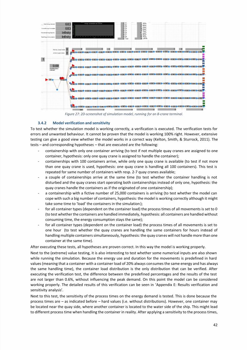
7/23/2019 Thesis Robert Heij Final Digital Version
http://slidepdf.com/reader/full/thesis-robert-heij-final-digital-version 42/94
42
Figure 27: 2D-screenshot of simulation model, running for an 8-crane terminal.
3.4.2
Model verification and sensitivityTo test whether the simulation model is working correctly, a verification is executed. The verification tests for
errors and unwanted behaviour. It cannot be proven that the model is working 100% right. However, extensive
testing can give a good view whether the model works in a correct way (Kelton, Smith, & Sturrock, 2011). The
tests – and corresponding hypotheses – that are executed are the following:
- containership with only one container arriving (to test if not multiple quay cranes are assigned to one
container, hypothesis: only one quay crane is assigned to handle the container);
- containerships with 100 containers arrive, while only one quay crane is available (to test if not more
than one quay crane is used, hypothesis: one quay crane is handling all 100 containers). This test is
repeated for same number of containers with resp. 2-7 quay cranes available;
- a couple of containerships arrive at the same time (to test whether the container handling is not
disturbed and the quay cranes start operating both containerships instead of only one, hypothesis: thequay cranes handle the containers as if the originated of one containership);
- a containership with a fictive number of 25,000 containers is arriving (to test whether the model can
cope with such a big number of containers, hypothesis: the model is working correctly although it might
take some time to ‘load’ the containers in the simulation );
- for all container types (dependent on the container load) the process times of all movements is set to 0
(to test whether the containers are handled immediately, hypothesis: all containers are handled without
consuming time, the energy consumption stays the same);
- for all container types (dependent on the container load) the process times of all movements is set to
one hour (to test whether the quay cranes are handling the same containers for hours instead of
handling multiple containers simultaneously, hypothesis: the quay cranes will not handle more than one
container at the same time).
After executing these tests, all hypotheses are proven correct. In this way the model is working properly.
Next to the (extreme) value testing, it is also interesting to test whether some numerical inputs are also shown
while running the simulation. Because the energy use and duration for the movements is predefined in hard
values (meaning that a container with a container load of 20% always consumes the same energy and has always
the same handling time), the container load distribution is the only distribution that can be verified. After
executing the verification test, the difference between the predefined percentages and the results of the test
are not larger than 0.6%, without influencing the peak demand. On this point the model can be considered
working properly. The detailed results of this verification can be seen in ‘Appendix E: Results verification and
sensitivity analysis’.
Next to this test, the sensitivity of the process times on the energy demand is tested. This is done because the
process times are – as indicated before – hard values (i.e. without distributions). However, one container may
be located near the quay side, where another container is located to the water side of the ship. This might leadto different process time when handling the container in reality. After applying a sensitivity to the process times,
7/23/2019 Thesis Robert Heij Final Digital Version
http://slidepdf.com/reader/full/thesis-robert-heij-final-digital-version 43/94
43
the result is that the distribution would have a difference of only 0.75% on the peak demand, meaning a cost
difference of only €3,700 per year. The conclusion is that the model is sensitive on this point, but the sensitivity
is not influencing the model outcome significantly. A more detailed explanation (including graphs) of the
numerical verification and sensitivity analysis, is presented in ‘Appendix E: Results verification and sensitivity
analysis’.
3.5
Model validation3.5.1 Design of experiments
Before the results of the base scenario (i.e. current situation without implemented rules of operation) can be
described and the model can be validated, a test run has to be done to determine the desired number of
replications that need to be executed to get reliable results out of the experiments for the developed rules of
operation. The test run is developed based on the theory of Van Soest (1992). Van Soest states that the desired
number of replications is dependent on the number of replications that is executed for the test run, the highest
observed value of performance variable and the corresponding half width of that variable. The formula is
visualised in equation 03.
. . ∗ ℎ ℎ ℎℎ ∗ 0.052 equation 03
In the test run with 10 replications, the highest observed value is 18,057 kW10. The half width of the peak demand
is 364.45, which gives a desired number of replications of 8, as can be seen in equation 04 below.
. 10 ∗ 364.4518,057 ∗0.052 8.1 equation 04
The result of this calculation is that the experiments that are executed to test the rules of operations (see chapter
4) need to be executed with eight replications per scenario.
The replication settings of Simio are such that replications are independent of each other. Each replication uses
a different set of random generated numbers (Kelton, Smith, & Sturrock, 2011). However, the same initial
preconditions are used to ensure the comparability of replications with each other.
3.5.2
Results base scenario
The base scenario of the simulation model is executed with the standard specifications of the container terminal.
This means that all eight quay cranes are handling containers, without any restrictions towards the number of
simultaneously lifting quay cranes or maximum energy demand per second. The base scenario is run with ten
replications (more than the minimum desired eight replications, as calculated in the last sub-paragraph). As
discussed earlier, the time span is one week. During this week 19 containerships arrive with a total of 10,057
containers (40ft. containers).
The average maximum energy demand of all replications is 19,177kW, with a minimum of 18,063kW and amaximum of 20,004kW. The corresponding half width is 364.4kW. The handling time of all containers is 1,857
minutes, which is 31.0 hours.
Figure 28 gives an overview of the energy demand frequency per 0.1 second. Here the idle times are neglected.
As can be seen, a maximum energy demand of 18,000+ kW is only consumed during a very small time period. An
energy demand higher than 9,000kW is observed in only 1.1% of the time. This endorses the hypothesis that the
highest peak demand can be reduced without influencing the operations too much.
10 The auxiliary energy consumption of quay cranes is not included in the output of the energy consumption. This means that
a peak demand of 18,057kW in the simulation model corresponds to a real peak demand of 19,177kW.

7/23/2019 Thesis Robert Heij Final Digital Version
http://slidepdf.com/reader/full/thesis-robert-heij-final-digital-version 44/94
44
Figure 28: Frequency graph for energy demand (measured per 0.1s)
3.5.3 Validation simulation model
The model validation is executed to check whether the energy consumption of containers in the simulation is
corresponding with real data. This is done for several criteria:
Energy demand
Each container load (0% - 100%) has its own pre-defined energy specifications (kW/s). Multiplied by the operation
times per sub-movement, the total energy consumption for a container can be determined. The theoretical
energy consumption (based on the data) is compared with the results of the simulation model. The result (see
Table 5) is that the maximum difference in energy consumption is 0.9%. For most container loads the difference
is not larger than 0.2%.
Table 5: Validation for energy demand of simulation model
Container
load
Energy demand
real data (kWh)
Energy demand
model (kWh) Difference
0% 2.12 2.12 0.00 (0.00%)20% 5.01 5.00 -0.01 (-0.20%)
30% 5.73 5.75 +0.02 (0.35%)
40% 6.26 6.25 -0.01 (-0.16%)
50% 5.05 5.05 0.00 (0.00%)
60% 4.44 4.48 +0.04 (+0.90%)
70% 4.76 4.78 +0.02 (+0.42%)
80% 4.87 4.86 -0.01 (-0.21%)
90% 4.86 4.86 0.00 (0.00%)
100% 5.20 5.20 0.00 (0.00%)
Because the different container loads are not appearing in the same proportion, the difference is multiplied withtheir appearance distribution (container mix). The results is a weighted difference of 0.26% (see Table 6 on next
page), which might be considered not significant to the energy consumption results. The influence on the energy
peak is however difficult to calculate, because that depends on the current container mix, which is changing
continuously in the simulation model.
0,0%
3,0%
6,0%
9,0%
12,0%
15,0%
- 1 2 . 0 0 0 , - 1 1 . 0 0 0
- 1 1 . 0 0 0 , - 1 0 . 0 0 0
- 1 0 . 0 0 0 , - 9 . 0 0 0
- 9 . 0 0 0 , - 8 . 0 0 0
- 8 . 0 0 0 , - 7 . 0 0 0
- 7 . 0 0 0 , - 6 . 0 0 0
- 6 . 0 0 0 , - 5 . 0 0 0
- 5 . 0 0 0 , - 4 . 0 0 0
- 4 . 0 0 0 , - 3 . 0 0 0
- 3 . 0 0 0 , - 2 . 0 0 0
- 2 . 0 0 0 , - 1 . 0 0 0
- 1 . 0 0 0 , 0
0 - 1 . 0 0 0
1 . 0 0 0 - 2 . 0 0 0
2 . 0 0 0 - 3 . 0 0 0
3 . 0 0 0 - 4 . 0 0 0
4 . 0 0 0 - 5 . 0 0 0
5 . 0 0 0 - 6 . 0 0 0
6 . 0 0 0 - 7 . 0 0 0
7 . 0 0 0 - 8 . 0 0 0
8 . 0 0 0 - 9 . 0 0 0
9 . 0 0 0 - 1 0 . 0 0 0
1 0 . 0 0 0 - 1 1 . 0 0 0
1 1 . 0 0 0 - 1 2 . 0 0 0
1 1 . 0 0 0 - 1 3 . 0 0 0
1 3 . 0 0 0 - 1 4 . 0 0 0
1 4 . 0 0 0 - 1 5 . 0 0 0
1 5 . 0 0 0 - 1 6 . 0 0 0
1 6 . 0 0 0 - 1 7 . 0 0 0
1 7 . 0 0 0 - 1 8 . 0 0 0
1 8 . 0 0 0 +
F r e q u e n c y
Energy demand (kW)

7/23/2019 Thesis Robert Heij Final Digital Version
http://slidepdf.com/reader/full/thesis-robert-heij-final-digital-version 45/94
45
Table 6: Weighted difference for difference in energy demand
Container
load
Container
mix Difference
Weighted
difference
0% 12.5% 0.00% 0.00%
20% 32.0% 0.20% 0.06%
30% 11.1% 0.35% 0.04%
40% 11.4% 0.16% 0.02%
50% 13.6% 0.00% 0.00%
60% 13.6% 0.90% 0.12%
70% 3.3% 0.42% 0.01%
80% 1.6% 0.21% 0.00%
90% 0.6% 0.00% 0.00%
100% 0.3% 0.00% 0.00%
Total weighted average 0.26%
Peak demandWhen comparing the peak demand of the simulation (base scenario with eight lifting quay cranes and no
restriction towards the maximum energy demand per second), the peak demand lies around 20,000kW. This is
consistent with data that of a terminal with eight quay cranes (ABB, 2014), which validates the outcome of the
simulation model on this aspect.
Handling time
The total run time for the base scenario is 171.0 hours (one week plus three hours extra run time). The quay
cranes are operating 18.0% of the time (half width 0.5%), which is 30.8 hours. In this time frame 10,057
containers are handled. Based on the fact that eight quay cranes are operating, resulting in a handling time of
88.1 seconds/container.
The theoretical (weighted) handling time of a container (based on the appearance of each container load) is 91.4
seconds/container, a difference of 3.3 seconds (3.6%). This difference could be explained by random distributionof process times for engaging the container in the simulation model, while the theoretical handling time makes
use of standard process times instead of a distribution.
3.6 Conclusion
When developing a consumption model for the dynamic representation of the electrical power consumption at
a container terminal, existing models do not satisfy the requirements for this visualisation. The consumption
model that is presented in this chapter makes a distinction between the different movements of terminal
equipment, since the energy consumption differs for each type of movement. Vertical movements (hoisting and
lowering the spreader and container) consume much more energy than horizontal gantry movements.
The consumption model showed that the electrical energy consumption of terminal equipment depends on the
different movements for transporting one or more containers (e.g. driving, lifting, lowering and gantry) and anauxiliary consumption. The consumption of terminal equipment (kW) can be calculated when having the
following information:
- Number of terminal equipment;
- Overview of different movements per type of equipment;
- Operational information (to determine at which moment a movement is executed);
- Energy consumption per movement (kW/s);
- Auxiliary energy consumption (kW/s).
The third sub-question – questioning whether it is feasible to develop a consumption model that takes into
account all relevant aspects of the electrical energy consumption of a container terminal and which shows the
consumption over time – can therefore be answered positive (see Figure 19 and equations 01 and 02).
For applying the consumption mode, a reliable data provider is needed, since the list of required data is ratherextensive. Especially because the required data is quite detailed at the point of the energy consumption of the
7/23/2019 Thesis Robert Heij Final Digital Version
http://slidepdf.com/reader/full/thesis-robert-heij-final-digital-version 46/94
46
different movements. This might be valuable information for container terminals, which they are not willing to
share. The more precise data that is obtained, the better the prediction of the consumption model. However,
when data is not available, assumptions need to be made in order to make an approximation of the energy
consumption. A disadvantage is that assumptions might harm the preciseness of the model results.
The presented model is not only useful for estimating the energy consumption for container terminals, it can
also be used in other industries where different electrical equipment is operating in different movements, e.g.
cranes and robots at construction sites or within factories. The same principle of dividing the equipment’s
operations into different movements can be applied easily and can help other industries to understand their
energy consumption (and see the peak demand and corresponding costs).
When applying the consumption model in a case-study for an existing container terminal, the best way to model
the container terminal operations and more specific the quay crane operations is using a discrete-event
simulation. The main reason for this is the event-based character of the simulation method. The assumptions
that were made to develop the simulation model influence the outcome of the simulation, but not for all
assumptions the exact influence is known. This means that the results of the simulation model should be
interpreted with this sensitivity in mind. The observed peak demand lies around the 20,000kW for a container
terminal with eight quay cranes. Chapter 4 presents the rules of operation that are developed to smoothen the
energy demand in order to lower the peak demand of 20,000kW. This peak alone costs a container terminal over
€500,000 per year, based on the price that grid operators charge per kW peak demand.
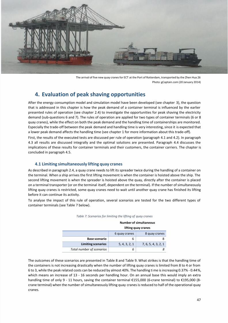
7/23/2019 Thesis Robert Heij Final Digital Version
http://slidepdf.com/reader/full/thesis-robert-heij-final-digital-version 47/94
47
The arrival of five new quay cranes for ECT at the Port of Rotterdam, transported by the Zhen Hua 26
Photo: gCaptain.com (20 January 2014)
4. Evaluation of peak shaving opportunities
After the energy consumption model and simulation model have been developed (see chapter 3), the question
that is addressed in this chapter is how the peak demand of a container terminal is influenced by the earlier
presented rules of operation (see chapter 2.4) to investigate the opportunities for peak shaving the electricitydemand (sub-questions 6 and 7). The rules of operation are applied for two types of container terminals (6 or 8
quay cranes), while the effect on both the peak demand and the handling time of containerships are monitored.
Especially the trade-off between the peak demand and handling time is very interesting, since it is expected that
a lower peak demand affects the handling time (see chapter 1 for more information about this trade-off).
First, the results of the executed tests are discussed per rule of operation (paragraph 4.1 and 4.2). In paragraph
4.3 all results are discussed integrally and the optimal solutions are presented. Paragraph 4.4 discusses the
implications of these results for container terminals and their customers, the container carriers. The chapter is
concluded in paragraph 4.5.
4.1 Limiting simultaneously lifting quay cranes
As described in paragraph 2.4, a quay crane needs to lift its spreader twice during the handling of a container onthe terminal. When a ship arrives the first lifting movement is when the container is hoisted above the ship. The
second lifting movement is when the spreader is hoisted above the quay, directly after the container is placed
on a terminal transporter (or on the terminal itself, dependent on the terminal). If the number of simultaneously
lifting quay cranes is restricted, some quay cranes need to wait until another quay crane has finished its lifting
before it can continue its activity.
To analyse the impact of this rule of operation, several scenarios are tested for the two different types of
container terminals (see Table 7 below).
Table 7: Scenarios for limiting the lifting of quay cranes
Number of simultaneous
lifting quay cranes
6 quay cranes 8 quay cranes
Base scenario 6 8
Limiting scenarios 5, 4, 3, 2, 1 7, 6, 5, 4, 3, 2, 1
Total number of scenarios 6 8
The outcomes of these scenarios are presented in Table 8 and Table 9. What strikes is that the handling time of
the containers is not increasing drastically when the number of lifting quay cranes is limited from 8 to 4 or from
6 to 3, while the peak related costs can be reduced by almost 40%. The handling time is increasing 0.37% - 0.44%,
which means an increase of 13 - 16 seconds per handling hour. On an annual base this would imply an extra
handling time of only 9 - 11 hours, saving the container terminal €155,000 (6-crane terminal) to €195,000 (8-
crane terminal) when the number of simultaneously lifting quay cranes is reduced to half of the operational quay
cranes.
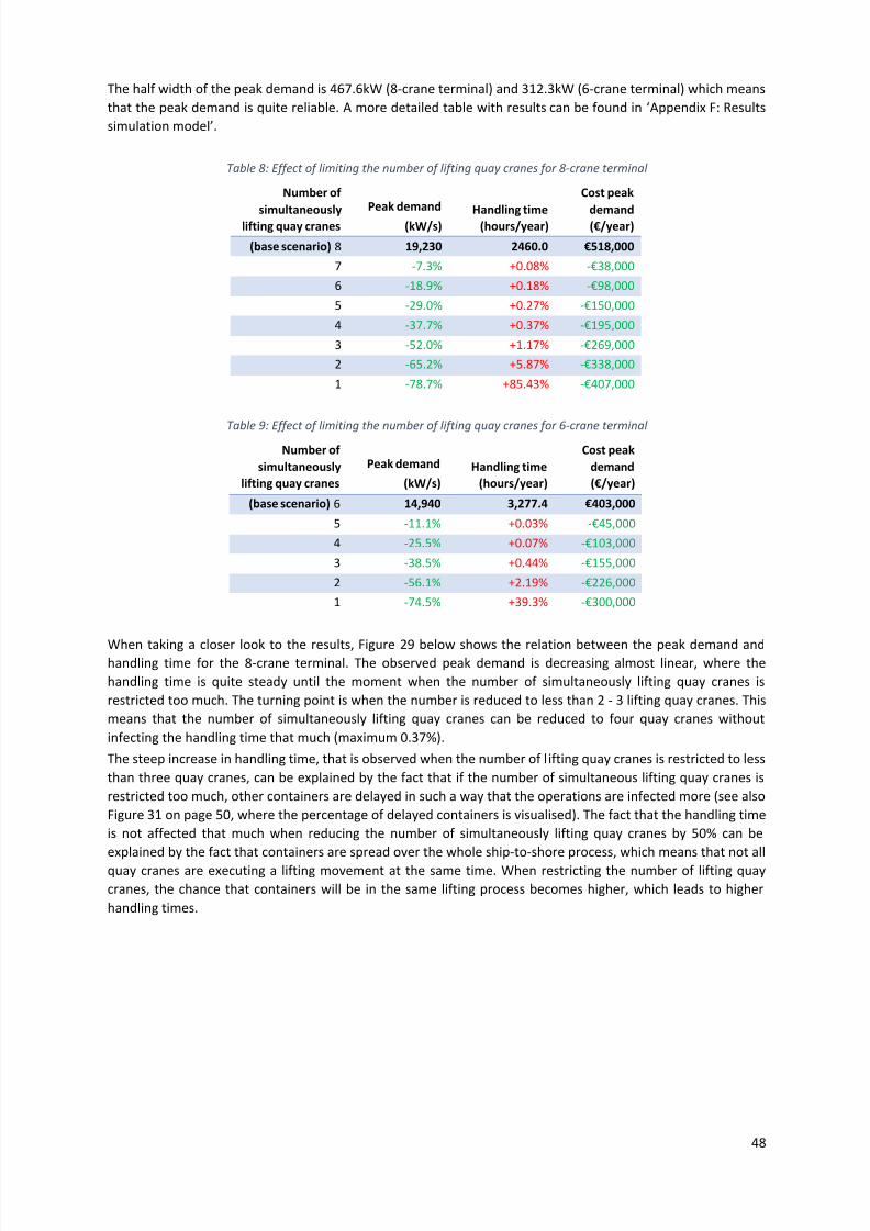
7/23/2019 Thesis Robert Heij Final Digital Version
http://slidepdf.com/reader/full/thesis-robert-heij-final-digital-version 48/94
48
The half width of the peak demand is 467.6kW (8-crane terminal) and 312.3kW (6-crane terminal) which means
that the peak demand is quite reliable. A more detailed table with results can be found in ‘Appendix F: Results
simulation model’.
Table 8: Effect of limiting the number of lifting quay cranes for 8-crane terminal
Number of
simultaneouslylifting quay cranes
Peak demand
(kW/s) Handling time(hours/year)
Cost peak
demand(€/year)
(base scenario) 8 19,230 2460.0 €518,000
7 -7.3% +0.08% -€38,000
6 -18.9% +0.18% -€98,000
5 -29.0% +0.27% -€150,000
4 -37.7% +0.37% -€195,000
3 -52.0% +1.17% -€269,000
2 -65.2% +5.87% -€338,000
1 -78.7% +85.43% -€407,000
Table 9: Effect of limiting the number of lifting quay cranes for 6-crane terminalNumber of
simultaneously
lifting quay cranes
Peak demand
(kW/s)
Handling time
(hours/year)
Cost peak
demand
(€/year)
(base scenario) 6 14,940 3,277.4 €403,000
5 -11.1% +0.03% -€45,000
4 -25.5% +0.07% -€103,000
3 -38.5% +0.44% -€155,000
2 -56.1% +2.19% -€226,000
1 -74.5% +39.3% -€300,000
When taking a closer look to the results, Figure 29 below shows the relation between the peak demand andhandling time for the 8-crane terminal. The observed peak demand is decreasing almost linear, where the
handling time is quite steady until the moment when the number of simultaneously lifting quay cranes is
restricted too much. The turning point is when the number is reduced to less than 2 - 3 lifting quay cranes. This
means that the number of simultaneously lifting quay cranes can be reduced to four quay cranes without
infecting the handling time that much (maximum 0.37%).
The steep increase in handling time, that is observed when the number of lifting quay cranes is restricted to less
than three quay cranes, can be explained by the fact that if the number of simultaneous lifting quay cranes is
restricted too much, other containers are delayed in such a way that the operations are infected more (see also
Figure 31 on page 50, where the percentage of delayed containers is visualised). The fact that the handling time
is not affected that much when reducing the number of simultaneously lifting quay cranes by 50% can be
explained by the fact that containers are spread over the whole ship-to-shore process, which means that not all
quay cranes are executing a lifting movement at the same time. When restricting the number of lifting quay
cranes, the chance that containers will be in the same lifting process becomes higher, which leads to higher
handling times.
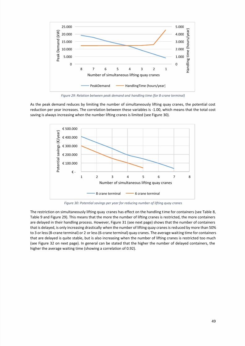
7/23/2019 Thesis Robert Heij Final Digital Version
http://slidepdf.com/reader/full/thesis-robert-heij-final-digital-version 49/94
49
Figure 29: Relation between peak demand and handling time (for 8-crane terminal)
As the peak demand reduces by limiting the number of simultaneously lifting quay cranes, the potential cost
reduction per year increases. The correlation between these variables is -1.00, which means that the total cost
saving is always increasing when the number lifting cranes is limited (see Figure 30).
Figure 30: Potential savings per year for reducing number of lifting quay cranes
The restriction on simultaneously lifting quay cranes has effect on the handling time for containers (see Table 8,
Table 9 and Figure 29). This means that the more the number of lifting cranes is restricted, the more containers
are delayed in their handling process. However, Figure 31 (see next page) shows that the number of containers
that is delayed, is only increasing drastically when the number of lifting quay cranes is reduced by more than 50%
to 3 or less (8-crane terminal) or 2 or less (6-crane terminal) quay cranes. The average waiting time for containers
that are delayed is quite stable, but is also increasing when the number of lifting cranes is restricted too much
(see Figure 32 on next page). In general can be stated that the higher the number of delayed containers, thehigher the average waiting time (showing a correlation of 0.92).
0
1.000
2.000
3.000
4.000
5.000
0
5.000
10.000
15.000
20.000
25.000
8 7 6 5 4 3 2 1 H a n d l i n g t i m e ( h o u r s / y e a r )
P
e a k D e m a n d ( k W )
Number of simultaneous lifting quay cranes
PeakDemand HandlingTime (hours/year)
€ -
€ 100.000
€ 200.000
€ 300.000
€ 400.000
€ 500.000
1 2 3 4 5 6 7 8
P o t e n t i a l s a v i n g s ( € / y e a r )
Number of simultaneous lifting quay cranes
8 crane terminal 6 crane terminal

7/23/2019 Thesis Robert Heij Final Digital Version
http://slidepdf.com/reader/full/thesis-robert-heij-final-digital-version 50/94
50
Figure 31: Percentage of delayed containers by reducing lifting quay cranes
Figure 32: Average waiting time for delayed containers
When dividing the total savings per year by the total extra handling time, the total savings per extra second
handling time can be determined. Figure 33 shows the result for this calculation. When looking to the 8-crane
terminal (blue line), the most cost-effective scenario is to reduce the number of lifting cranes to 6, 5 or 4. In case
of the 6-crane terminal, it is most cost-effective to reduce the number of lifting quay cranes to 5 or 4. In case of
reducing the number of quay cranes to resp. 6, 5 or 4 (8-crane terminal) or to 5 or 4 (6-crane terminal), the
chance that a container is delayed temporarily is between 0.3% - 5.7% (with an average waiting time of 0.02 -
0.17 seconds). The impact of this waiting of containers is considered limited due to the short waiting times and
low number of waiting containers.
Figure 33: Savings per second extra handling time.
0%
20%
40%
60%
80%
100%
1 2 3 4 5 6 7 8
W
a i t i n g c o n t a i n e r s
Number of simultaneous lifting quay cranes
8 crane terminal 6 crane terminal
0,0
10,0
20,0
30,0
40,0
1 2 3 4 5 6 7 8
A v e r a g e w a i t i n g
t i m e
( s e c o n d s / d e l a y e d c o n t a i n e r )
Number of simultaneous lifting quay cranes
8 crane terminal 6 crane terminal
€ 0,00
€ 2,00
€ 4,00
€ 6,00
€ 8,00
€ 10,00
€ 12,00
€ 14,00
€ 16,00
1 2 3 4 5 6 7 8
S a v i n g s p e r s e c o n d e x t r a h a n d l i n
g
t i m e ( € / s e c . / y e a r )
Number of simultaneous lifting quay cranes
8 crane terminal 6 crane terminal

7/23/2019 Thesis Robert Heij Final Digital Version
http://slidepdf.com/reader/full/thesis-robert-heij-final-digital-version 51/94
51
Conclusion
As concluded in this paragraph, restricting the number of simultaneously lifting quay cranes has a positive
influence on the reduction of the peak demand. In this way the restriction of lifting quay cranes can be
implemented in an operational environment to support container terminals to save costs against a relative low
increase of handling time. A restriction which allows only half of the operational quay cranes to lift
simultaneously has a limited effect on the handling time (maximum 0.44%), but saves the terminal up to
€155,000 - €195,000 per year, which is approximately 40% of the peak related energy costs.
Because the waiting time increases exponential when limiting the number of simultaneously lifting quay cranes
to more than half of the operational quay cranes, this seems no good idea. When looking to the savings per extra
second handling time (see Figure 33), the potential savings per second decrease rapidly when reducing the
number of simultaneously lifting quay cranes by more than 50%.
When looking to the most cost-effective scenario (i.e. yearly savings per extra second handling time) the most
optimal implementation is to reduce the number of lifting quay cranes to 6, 5 or 4 (8-crane terminal) or to 5 or 4
(6-crane terminal) as can be seen in Table 10. In these cases the savings per extra second handling time are higher
than for other scenarios. The 8-crane terminal is able to save €5.92-6.24 per second (total savings are €98,000 -
€195,000 per year, which is 19% - 38% of the peak related costs), the 6-crane terminal might save €13.08 - €14.67
per year (total savings are €45,000 - €103,000 per year, which is 11% - 26% of the total peak related costs).
Table 10: Best scoring scenarios based on impact on handling time and savings per second
Low impact on handling time
Number
of lifting
cranes
Total yearly
savings (€/year)
Savings per
extra second
(€/sec./year)
Extra
handling
time
Percentage
of waiting
containers
Average waiting time
waiting (sec./waiting
container)
8 cranes 4 € 195,000 (-38%) € 5.92 0.37% 5.70% 2.88
6 cranes 3 € 155,000 (-39%) € 2.96 0.44% 7.20% 2.76
Savings per extra second
Number
of lifting
cranes
Total yearly
savings (€/year)
Savings per
extra second
(€/sec./year)
Extra
handling
time
Percentage
of waiting
containers
Average waiting time
waiting (sec./waiting
container)
8 cranes
6 € 98,000 (-19%) € 6.24 0.18% 0.60% 5.41
5 € 150,000 (-29%) € 6.18 0.27% 1.60% 3.86
4 € 195,000 (-38%) € 5.92 0.37% 5.70% 2.88
6 cranes5 € 45,000 (-11%) € 14.67 0.03% 0.30% 5.48
4 € 103,000 (-26%) € 13.08 0.07% 1.70% 3.35
4.2 Limiting maximum energy demand
The restraining of energy demand contains the continuous checking of quay cranes whether they there is enough
energy demand left to continue its operations. When for example a quay crane needs 1000kW and only 500kW
is available due to the imposed maximum, the quay crane needs to wait until in total 500kW become available11.
When analysing this rule of operation, the number of simultaneously lifting quay cranes is not restricted. The
number of scenarios is determined by the highest peak demand that is observed for the 8-crane terminal (i.e.
19,200kW) and the 6-crane terminal (i.e. 14,940 kW). The lowest restriction is set at 4,000kW, since the
maximum energy demand for one movement (i.e. the lifting of a spreader and 100% loaded container above the
ships) is almost 3,000kW. A maximum allowed energy demand of 3,000kW would therefore delay the operations
severely.
11 The simulation model is constructed in such a way that when a quay crane needs 1000kW and only 500kW is available, theavailable 500kW is ‘seized’ (i.e. reserved for this quay crane). After that the quay crane is seizing the first available extra
500kW, whereupon it can continue its operations.
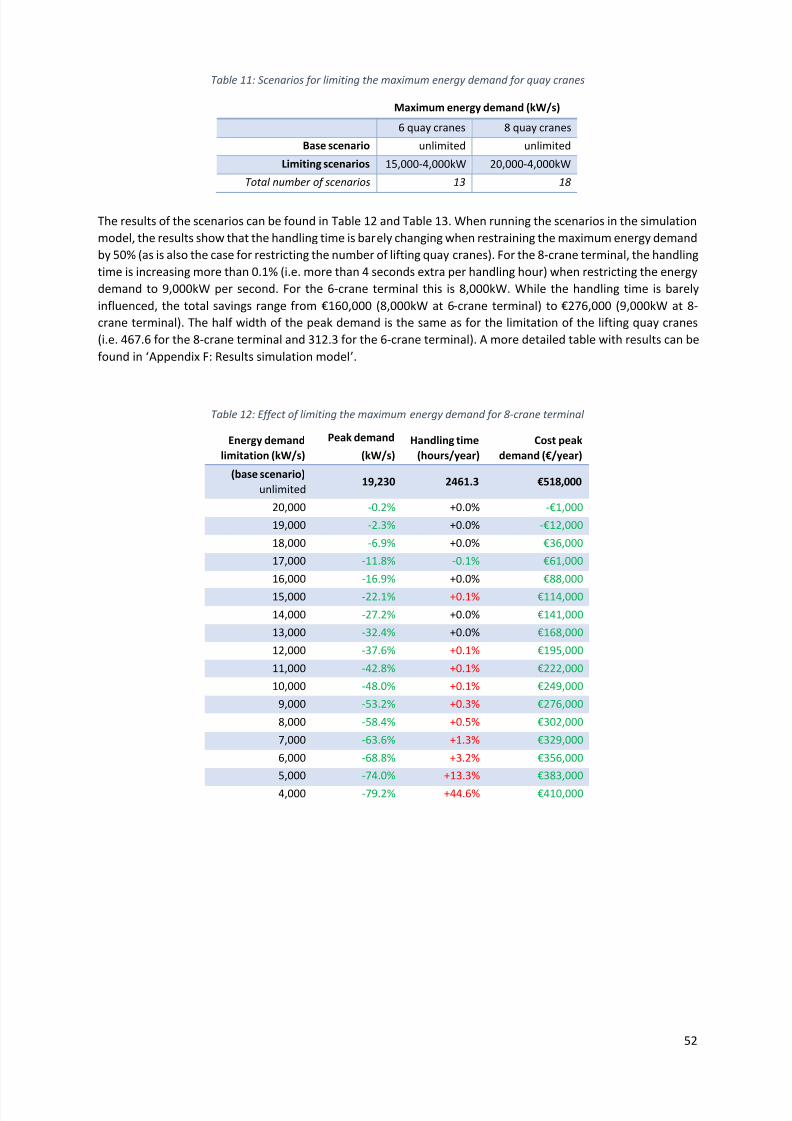
7/23/2019 Thesis Robert Heij Final Digital Version
http://slidepdf.com/reader/full/thesis-robert-heij-final-digital-version 52/94
52
Table 11: Scenarios for limiting the maximum energy demand for quay cranes
Maximum energy demand (kW/s)
6 quay cranes 8 quay cranes
Base scenario unlimited unlimited
Limiting scenarios 15,000-4,000kW 20,000-4,000kW
Total number of scenarios 13 18
The results of the scenarios can be found in Table 12 and Table 13. When running the scenarios in the simulation
model, the results show that the handling time is barely changing when restraining the maximum energy demand
by 50% (as is also the case for restricting the number of lifting quay cranes). For the 8-crane terminal, the handling
time is increasing more than 0.1% (i.e. more than 4 seconds extra per handling hour) when restricting the energy
demand to 9,000kW per second. For the 6-crane terminal this is 8,000kW. While the handling time is barely
influenced, the total savings range from €160,000 (8,000kW at 6-crane terminal) to €276,000 (9,000kW at 8-
crane terminal). The half width of the peak demand is the same as for the limitation of the lifting quay cranes
(i.e. 467.6 for the 8-crane terminal and 312.3 for the 6-crane terminal). A more detailed table with results can be
found in ‘Appendix F: Results simulation model’.
Table 12: Effect of limiting the maximum energy demand for 8-crane terminal
Energy demand
limitation (kW/s)
Peak demand
(kW/s)
Handling time
(hours/year)
Cost peak
demand (€/year)
(base scenario)
unlimited 19,230 2461.3 €518,000
20,000 -0.2% +0.0% -€1,000
19,000 -2.3% +0.0% -€12,000
18,000 -6.9% +0.0% €36,000
17,000 -11.8% -0.1% €61,000
16,000 -16.9% +0.0% €88,000
15,000 -22.1% +0.1% €114,000
14,000 -27.2% +0.0% €141,000
13,000 -32.4% +0.0% €168,000
12,000 -37.6% +0.1% €195,000
11,000 -42.8% +0.1% €222,000
10,000 -48.0% +0.1% €249,000
9,000 -53.2% +0.3% €276,000
8,000 -58.4% +0.5% €302,000
7,000 -63.6% +1.3% €329,000
6,000 -68.8% +3.2% €356,000
5,000 -74.0% +13.3% €383,000
4,000 -79.2% +44.6% €410,000
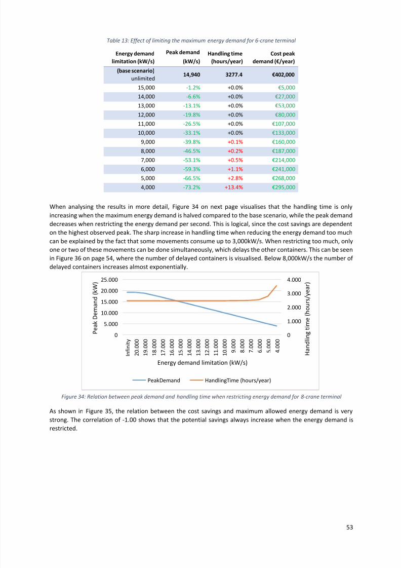
7/23/2019 Thesis Robert Heij Final Digital Version
http://slidepdf.com/reader/full/thesis-robert-heij-final-digital-version 53/94
53
Table 13: Effect of limiting the maximum energy demand for 6-crane terminal
Energy demand
limitation (kW/s)
Peak demand
(kW/s)
Handling time
(hours/year)
Cost peak
demand (€/year)
(base scenario)
unlimited 14,940 3277.4 €402,000
15,000 -1.2% +0.0% €5,000
14,000 -6.6% +0.0% €27,00013,000 -13.1% +0.0% €53,000
12,000 -19.8% +0.0% €80,000
11,000 -26.5% +0.0% €107,000
10,000 -33.1% +0.0% €133,000
9,000 -39.8% +0.1% €160,000
8,000 -46.5% +0.2% €187,000
7,000 -53.1% +0.5% €214,000
6,000 -59.3% +1.1% €241,000
5,000 -66.5% +2.8% €268,000
4,000 -73.2% +13.4% €295,000
When analysing the results in more detail, Figure 34 on next page visualises that the handling time is only
increasing when the maximum energy demand is halved compared to the base scenario, while the peak demand
decreases when restricting the energy demand per second. This is logical, since the cost savings are dependent
on the highest observed peak. The sharp increase in handling time when reducing the energy demand too much
can be explained by the fact that some movements consume up to 3,000kW/s. When restricting too much, only
one or two of these movements can be done simultaneously, which delays the other containers. This can be seen
in Figure 36 on page 54, where the number of delayed containers is visualised. Below 8,000kW/s the number of
delayed containers increases almost exponentially.
Figure 34: Relation between peak demand and handling time when restricting energy demand for 8-crane terminal
As shown in Figure 35, the relation between the cost savings and maximum allowed energy demand is very
strong. The correlation of -1.00 shows that the potential savings always increase when the energy demand is
restricted.
0
1.000
2.000
3.000
4.000
0
5.000
10.000
15.000
20.000
25.000
I n f i n i t y
2 0 . 0 0 0
1 9 . 0 0 0
1 8 . 0 0 0
1 7 . 0 0 0
1 6 . 0 0 0
1 5 . 0 0 0
1 4 . 0 0 0
1 3 . 0 0 0
1 2 . 0 0 0
1 1 . 0 0 0
1 0 . 0 0 0
9 . 0 0 0
8 . 0 0 0
7 . 0 0 0
6 . 0 0 0
5 . 0 0 0
4 . 0 0 0
H a n d l i n g t i m e ( h o u r s / y e a r )
P e a k D e m a n d
( k W )
Energy demand limitation (kW/s)
PeakDemand HandlingTime (hours/year)
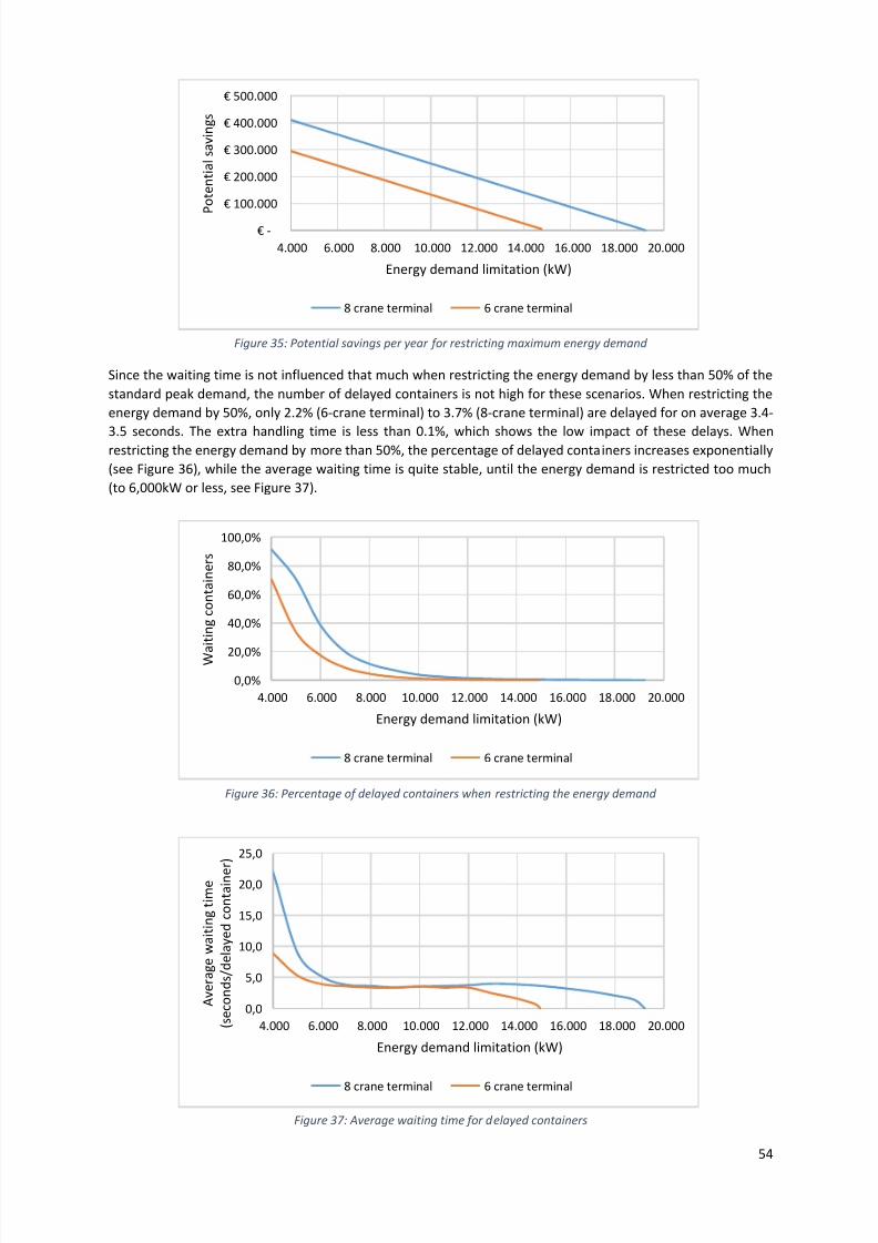
7/23/2019 Thesis Robert Heij Final Digital Version
http://slidepdf.com/reader/full/thesis-robert-heij-final-digital-version 54/94
54
Figure 35: Potential savings per year for restricting maximum energy demand
Since the waiting time is not influenced that much when restricting the energy demand by less than 50% of the
standard peak demand, the number of delayed containers is not high for these scenarios. When restricting the
energy demand by 50%, only 2.2% (6-crane terminal) to 3.7% (8-crane terminal) are delayed for on average 3.4-
3.5 seconds. The extra handling time is less than 0.1%, which shows the low impact of these delays. Whenrestricting the energy demand by more than 50%, the percentage of delayed containers increases exponentially
(see Figure 36), while the average waiting time is quite stable, until the energy demand is restricted too much
(to 6,000kW or less, see Figure 37).
Figure 36: Percentage of delayed containers when restricting the energy demand
Figure 37: Average waiting time for delayed containers
€ -
€ 100.000
€ 200.000
€ 300.000
€ 400.000
€ 500.000
4.000 6.000 8.000 10.000 12.000 14.000 16.000 18.000 20.000
P o t e n t i a l s a v i n g s
Energy demand limitation (kW)
8 crane terminal 6 crane terminal
0,0%
20,0%
40,0%
60,0%
80,0%
100,0%
4.000 6.000 8.000 10.000 12.000 14.000 16.000 18.000 20.000
W a i t i n g c o n t a i n e r s
Energy demand limitation (kW)
8 crane terminal 6 crane terminal
0,0
5,0
10,0
15,0
20,0
25,0
4.000 6.000 8.000 10.000 12.000 14.000 16.000 18.000 20.000
A v e r a g e w a i t i n g t i m e
( s e c o n d s / d e l a y e d c o n t a i n e
r )
Energy demand limitation (kW)
8 crane terminal 6 crane terminal

7/23/2019 Thesis Robert Heij Final Digital Version
http://slidepdf.com/reader/full/thesis-robert-heij-final-digital-version 55/94
55
When the total savings per year are divided by the extra handling time that is needed to handle all containers on
a yearly base, the savings per second are obtained, as shown by Figure 38. For the 8-crane terminal there is a
clear optimum when reducing the maximum demand to 14,000kW. In this case the savings are €141,000 per
year, while the handling time is 0.01% faster. This results in a negative saving12 of €197.10 per second. Restricting
the energy demand to 17,000kW, 18,000kW or 19,000kW results also in a negative saving. However, in these
cases the total savings are only €12,000 to €61,000. Restricting the energy demand to 13,000kW gives a saving
of €251.53 per second, which the absolutely seen the highest saving.
For the 6-crane terminal the highest (negative) saving per second is obtained by reducing the maximum energy
demand to 12,000kW (-€180.27 per second) or 13,000kW (-€115.86 per second), saving the terminal resp.
€80,000 or €53,000 per year. The highest positive value (meaning a saving against extra handling time) is
achieved by reducing the energy demand to 11,000kW. This saves €79.40 per second against an extra handling
time of 0.01% and a total cost saving of €107,000.
Figure 38: Savings per second extra handling time.
ConclusionDerived from the described figures and tables, it can be concluded that decreasing the maximum allowed energy
demand has a positive influence on the reduction of the terminals’ peak demand. The influence on the handling
time is only minimal when reducing the allowed energy demand by approximately 50%, while it enables container
terminals to reduce their peak related energy costs by the same percentage, up to €250,000 per year. All results
can be seen in Table 14.
When focusing on the most cost-effective result (i.e. yearly savings per extra second handling time) the most
optimal implementation is to reduce the maximum energy demand to 14,000kW or 13,000kW for the 8-crane
and to 13,000kW or 12,000 kW for the 6-crane terminals. For the 8-crane terminal this implies a negative saving
of €197.10 per second or a saving of €251.53 per extra second, up to €168,000/year in total.
For the 6-crane terminal a reduction to 13,000kW or 12,000kW are a less cost-effective and the total savings are
also relatively low (13% - 20% compared to the 27% - 32% of the 8-crane terminal). The handling time is hardly
increasing, while the number of containers that is delayed by these scenarios is less than 0.3%.
12 The negative cost saving per second is actually a positive result, since the handling time for this scenario is lower comparedto the standard situation, which means that the cost savings (positive result) are divided by a negative extra handling time
(i.e. less handling time).
-€ 300
-€ 200
-€ 100
€ 0
€ 100
€ 200
€ 300
4.000 6.000 8.000 10.000 12.000 14.000 16.000 18.000 20.000
S a v i n g s p e r s e c o n d e x t r a h a n d l i n g
t i m e ( € / s e c . /
y e a r )
Energy demand limitation (kW)
8 crane terminal 6 crane terminal
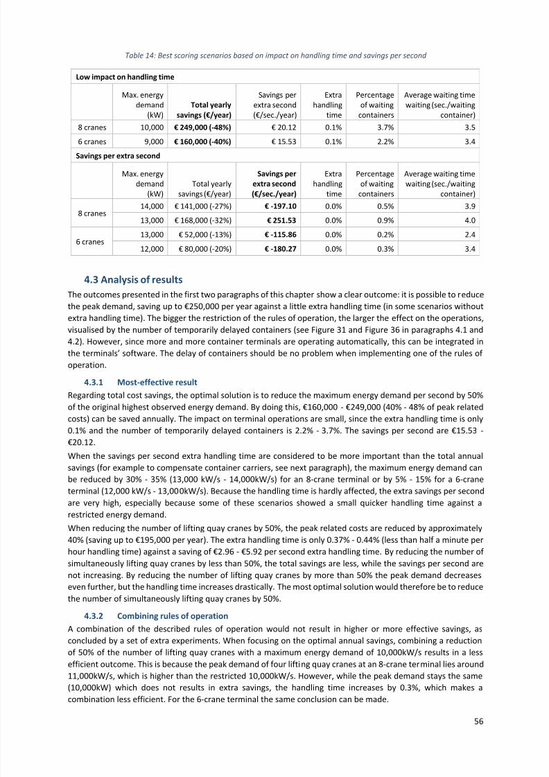
7/23/2019 Thesis Robert Heij Final Digital Version
http://slidepdf.com/reader/full/thesis-robert-heij-final-digital-version 56/94
56
Table 14: Best scoring scenarios based on impact on handling time and savings per second
Low impact on handling time
Max. energy
demand
(kW)
Total yearly
savings (€/year)
Savings per
extra second
(€/sec./year)
Extra
handling
time
Percentage
of waiting
containers
Average waiting time
waiting (sec./waiting
container)
8 cranes 10,000 € 249,000 (-48%) € 20.12 0.1% 3.7% 3.5
6 cranes 9,000 € 160,000 (-40%) € 15.53 0.1% 2.2% 3.4
Savings per extra second
Max. energy
demand
(kW)
Total yearly
savings (€/year)
Savings per
extra second
(€/sec./year)
Extra
handling
time
Percentage
of waiting
containers
Average waiting time
waiting (sec./waiting
container)
8 cranes14,000 € 141,000 (-27%) € -197.10 0.0% 0.5% 3.9
13,000 € 168,000 (-32%) € 251.53 0.0% 0.9% 4.0
6 cranes13,000 € 52,000 (-13%) € -115.86 0.0% 0.2% 2.4
12,000 € 80,000 (-20%) € -180.27 0.0% 0.3% 3.4
4.3
Analysis of results
The outcomes presented in the first two paragraphs of this chapter show a clear outcome: it is possible to reduce
the peak demand, saving up to €250,000 per year against a little extra handling time (in some scenarios without
extra handling time). The bigger the restriction of the rules of operation, the larger the effect on the operations,
visualised by the number of temporarily delayed containers (see Figure 31 and Figure 36 in paragraphs 4.1 and
4.2). However, since more and more container terminals are operating automatically, this can be integrated in
the terminals’ software. The delay of containers should be no problem when implementing one of the rules of
operation.
4.3.1 Most-effective result
Regarding total cost savings, the optimal solution is to reduce the maximum energy demand per second by 50%
of the original highest observed energy demand. By doing this, €160,000 - €249,000 (40% - 48% of peak relatedcosts) can be saved annually. The impact on terminal operations are small, since the extra handling time is only
0.1% and the number of temporarily delayed containers is 2.2% - 3.7%. The savings per second are €15.53 -
€20.12.
When the savings per second extra handling time are considered to be more important than the total annual
savings (for example to compensate container carriers, see next paragraph), the maximum energy demand can
be reduced by 30% - 35% (13,000 kW/s - 14,000kW/s) for an 8-crane terminal or by 5% - 15% for a 6-crane
terminal (12,000 kW/s - 13,000kW/s). Because the handling time is hardly affected, the extra savings per second
are very high, especially because some of these scenarios showed a small quicker handling time against a
restricted energy demand.
When reducing the number of lifting quay cranes by 50%, the peak related costs are reduced by approximately
40% (saving up to €195,000 per year). The extra handling time is only 0.37% - 0.44% (less than half a minute per
hour handling time) against a saving of €2.96 - €5.92 per second extra handling time. By reducing the number of
simultaneously lifting quay cranes by less than 50%, the total savings are less, while the savings per second are
not increasing. By reducing the number of lifting quay cranes by more than 50% the peak demand decreases
even further, but the handling time increases drastically. The most optimal solution would therefore be to reduce
the number of simultaneously lifting quay cranes by 50%.
4.3.2 Combining rules of operation
A combination of the described rules of operation would not result in higher or more effective savings, as
concluded by a set of extra experiments. When focusing on the optimal annual savings, combining a reduction
of 50% of the number of lifting quay cranes with a maximum energy demand of 10,000kW/s results in a less
efficient outcome. This is because the peak demand of four lifting quay cranes at an 8-crane terminal lies around
11,000kW/s, which is higher than the restricted 10,000kW/s. However, while the peak demand stays the same
(10,000kW) which does not results in extra savings, the handling time increases by 0.3%, which makes a
combination less efficient. For the 6-crane terminal the same conclusion can be made.

7/23/2019 Thesis Robert Heij Final Digital Version
http://slidepdf.com/reader/full/thesis-robert-heij-final-digital-version 57/94
57
When looking to the most optimal results for the highest savings per second, a reduction to five or sixlifting quay
cranes at an 8-crane terminal leads to a peak demand of 13,500 - 15,500kW/s, which is higher than the optimal
restriction in energy demand (13,000 - 14,000kW/s). Again the same conclusions can be made for the 6-crane
terminal.
4.4 Implications of results
4.4.1
Extra handling time
The last paragraphs showed the financial benefits for container terminal when the energy demand or number of
simultaneously lifting quay cranes is restricted. The handling time does not increase per se, however, a slight
increase is to be expected. This means that the container terminals take the benefit of a lower energy bill, while
the container carriers are the ones that have to accept extra handling time. The question is whether container
carriers accept this extra handling time, since the benefits are fully for the container terminal while the
disadvantage is for their account.
Extra waiting time for containerships is something that is watched critically by the container carriers. Shells
Maritime Efficiency Manager, Leendert van den Ende, stated that unnecessary waiting time involves extra costs
for them as charterer (Port of Rotterdam, 2013). Despite the critical attitude of cargo carriers towards waiting
time in ports, the adaption of containerships’ cruising speeds (also known as slow steaming) is no issue. For
container carriers, their biggest costs are fuel. These costs might be reduced by adapting the ship speed: areduction to 80% saves 60% fuel costs, while a reduction to 60% saves 90% of the fuel costs (Wärtsilä, 2010). A
market survey showed that 75% of the surveyed liners and carriers apply slow steaming in order to save bunker
costs (Seatrade Global, 2014). Since the fuel costs are that high, container carriers are operating more efficient
when sailing at lower speeds. In this regard the extra travel time is compensated by fuel savings.
4.4.2 Costs containership
For handling 2,000 TEU of a containership (loading and unloading) a terminal needs approximately 18 hours using
only three quay cranes. When extra handling time is needed, the question is whether container carriers are
willing to accept this without any form of compensation. If terminal operations take more time than agreed in
advance, carriers are compensated, known as demurrage (Haugen Consulting, 2015). When a ship requires less
time than agreed on forehand, the terminal can request a bonus for quicker handling, the so called despatch.
This shows that compensation is quite regular in the shipping business.The question is therefore whether container terminals are able to compensate container carriers to a certain
extent. To answer this question, first the costs for a containership need to be determined. To determine the
annual costs for a containership, AECOM made a report for the North Carolina Department of Transportation
(2012). They pointed out three cost aspects: the investment costs for a containership, labour costs and fuel costs.
The purchase of a containership of 15,000 TEU (Emma Maersk class) costs around 127 million euros (Maersk,
2006). When dividing these costs over a lifespan of 30 years and an annual discount rate of six percent, this
results in around 9 million euros per year. The labour costs can be estimated at 1.2 million euros (AECOM, 2012).
Fuel costs can be neglected, since extra handling time will not lead to extra fuel consumption.
Table 15: Cost containership per year, hour and second
Type of cost Costs
Investment costs € 9,000,000 Labour costs € 1,200,000
Total per year € 10,200,000
Total per hour € 1,164
Total per second € 0.32
Since a peak reduction of 50% saves a container terminal at least €2.96-5.92 per second (see paragraph 4.3.1),
this leaves room to compensate the carriers for the extra handling time. This could result in a win-win situation:
container terminals saving costs by reducing their peak demand and carriers reducing their handling costs due
to the compensation.

7/23/2019 Thesis Robert Heij Final Digital Version
http://slidepdf.com/reader/full/thesis-robert-heij-final-digital-version 58/94
58
4.5 Conclusion
The two rules of operations that are tested on their contribution to reduce the peak demand, showed that the
peak demand can be reduced by almost 50%, while the handling time is only increasing slightly with maximum
half a minute per hour handling time. This can be achieved by limiting the maximum energy demand to 50% of
the peak demand that is observed in the normal situation (i.e. without restrictions of one or more rules of
operation).
By restricting the maximum energy demand per second, a container terminal is able to set a ceiling on the energydemand, which means that each quay crane needs to get ‘permission’ before executing one of its movements. If
there is not enough energy left to execute a particular movement, a container is temporarily delayed. However,
the percentage of containers that is temporarily delayed is less than 3.7% when reducing the energy demand
limit by 50%.
The limitation of simultaneously lifting quay cranes is also successful to reduce peak demand. Most savings are
achieved by reducing the number of simultaneously lifting cranes to 50% of the total number of cranes at the
container terminal. However, the savings for this rule of operation are 10% lower than for limiting the energy
demand. Next to that, the impact on operations (percentage of delayed containers) is 5.7%, which is 2.0% higher
than for limiting the energy demand by 50%.
In this way, both rules of operation can be recommended for peak shaving the electricity demand at container
terminals (sub-question 7). However, the restriction on the maximum energy demand is able to reduce the costs
by 50% without influencing the handling time by more than half a minute per hour handling time.

7/23/2019 Thesis Robert Heij Final Digital Version
http://slidepdf.com/reader/full/thesis-robert-heij-final-digital-version 59/94
59
Barges and large containership docked at the Euromax terminal, Port of Rotterdam
Photo: Marijn van Hoorn (Flickr, 28 June 2012)
5. Conclusions and recommendations
In this research the container terminal operations are discussed (chapter 2), leading to the development of an
energy consumption model and a simulation model (chapter 3). The results of the simulation study are
subsequently described and discussed (chapter 4). In this chapter the research is concluded in paragraph 5.1, presenting the most remarkable findings. Based on the findings of this research, several recommendations and
directions for future research are given in paragraphs 5.2 and 5.3.
5.1 Conclusions
The research has shown that it is possible to smoothen the peak demand of a container terminal by implementing
rules of operation. These rules act as ‘controllers’ that smoothen the energy demand by limiting the cause of
high peaks. Two rules are studied: less quay cranes that lift simultaneously and limiting the movements of quay
cranes by putting a maximum on the energy demand per second).
The effects of the suggested rules of operation can be measured in two ways13:
- Maximum total savings for terminal
Finding the optimum of cost savings based on savings and acceptable14 extra handling time.- Cost-effectiveness terminal
Finding the maximum savings based on savings per extra second handling time.
When applying the energy consumption model for a container terminal with 6-8 quay cranes, the following
results are shown for the two tested rules of operation:
Limiting simultaneously lifting quay cranes
The number of simultaneously lifting quay cranes can be reduced by 50%, impacting the handling time less than
0.5%. By reducing the number of simultaneously lifting quay cranes to 50%, a peak shaving and cost reduction of
39% can be achieved, as shown by Table 16. The impact on operations is then maximum 0.44%. The number of
simultaneously can be reduced even more, but the handling time would then increase exponentially and almost
one out of five containers would be delayed temporarily. By reducing the number of simultaneously lifting quay
cranes by 50%, one out of 20 containers would be delayed temporarily. This shows that terminal operations are
quite stable when reducing the number of simultaneously lifting quay cranes by 50%. This is understandable
since not all quay cranes are continuously executing a lifting movement at the same time. The restriction is
therefore not restricting quay cranes during the whole time of operations.
When focussing on the savings per second, an optimum is found when reducing the number of simultaneously
lifting quay cranes to 6 cranes (8-crane terminal) or 5 cranes (6-crane terminal). In these scenarios the peak
13 The savings are derived from the reduction in peak demand; the higher the savings, the higher the reduction
in peak demand). A reduction of 10% in peak demand returns a cost saving of 10%. In most situation the cost
savings will be described, since the ultimate objective for container terminals is to reduce their peak-related
costs.14 When one only focuses on cost reduction, the peak demand can be reduced in such a way that the handling time is
increasing enormously. Therefore a certain ‘limit’ has to be set, to find a feasible result.
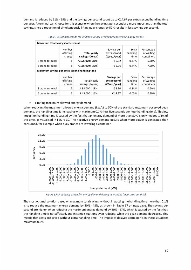
7/23/2019 Thesis Robert Heij Final Digital Version
http://slidepdf.com/reader/full/thesis-robert-heij-final-digital-version 60/94
60
demand is reduced by 11% - 19% and the savings per second count up to €14.67 per extra second handling time
per year. A terminal can choose for this scenario when the savings per second are more important than the total
savings, since a reduction of simultaneously lifting quay cranes by 50% results in less savings per second.
Table 16: Optimal results for limiting number of simultaneously lifting quay cranes
Maximum total savings for terminal
Number
of lifting
cranes
Total yearly
savings (€/year)
Savings per
extra second
(€/sec./year)
Extra
handling
time
Percentage
of waiting
containers
8 crane terminal 4 € 195,000 (-38%) € 5.92 0.37% 5.70%
6 crane terminal 3 € 155,000 (-39%) € 2.96 0.44% 7.20%
Maximum savings per extra second handling time
Number
of lifting
cranes
Total yearly
savings (€/year)
Savings per
extra second
(€/sec./year)
Extra
handling
time
Percentage
of waiting
containers
8 crane terminal 6 € 98,000 (-19%) € 6.24 0.18% 0.60%
6 crane terminal 5 € 45,000 (-11%) € 14.67 0.03% 0.30%
Limiting maximum allowed energy demand
When reducing the maximum allowed energy demand (kW/s) to 50% of the standard maximum observed peak
demand, the handling time is increasing with maximum 0.1% (less five seconds per hour handling time). This low
impact on handling time is caused by the fact that an energy demand of more than 50% is only needed 1.1% of
the time, as visualised in Figure 39. The negative energy demand occurs when more power is generated than
consumed, for example when quay cranes are lowering a container.
Figure 39: Frequency graph for energy demand during operations (measured per 0.1s)
The most optimal solution based on maximum total savings without impacting the handling time more than 0.1%
is to reduce the maximum energy demand by 40% - 48%, as shown in Table 17 on next page. The savings per
second are higher when reducing the maximum energy demand by 20% - 27%, which is caused by the fact that
the handling time is not affected, and in some situations even reduced, while the peak demand decreases. This
means that costs are saved without extra handling time. The impact of delayed container is in these situations
maximum 0.5%.
0,0%
3,0%
6,0%
9,0%
12,0%
15,0%
- 1 2 . 0 0 0 , - 1 1 . 0 0 0
- 1 1 . 0 0 0 , - 1 0 . 0 0 0
- 1 0 . 0 0 0 , - 9 . 0 0 0
- 9 . 0 0 0 , - 8 . 0 0 0
- 8 . 0 0 0 , - 7 . 0 0 0
- 7 . 0 0 0 , - 6 . 0 0 0
- 6 . 0 0 0 , - 5 . 0 0 0
- 5 . 0 0 0 , - 4 . 0 0 0
- 4 . 0 0 0 , - 3 . 0 0 0
- 3 . 0 0 0 , - 2 . 0 0 0
- 2 . 0 0 0 , - 1 . 0 0 0
- 1 . 0 0 0 , 0
0 - 1 . 0 0 0
1 . 0 0 0 - 2 . 0 0 0
2 . 0 0 0 - 3 . 0 0 0
3 . 0 0 0 - 4 . 0 0 0
4 . 0 0 0 - 5 . 0 0 0
5 . 0 0 0 - 6 . 0 0 0
6 . 0 0 0 - 7 . 0 0 0
7 . 0 0 0 - 8 . 0 0 0
8 . 0 0 0 - 9 . 0 0 0
9 . 0 0 0 - 1 0 . 0 0 0
1 0 . 0 0 0 - 1 1 . 0 0 0
1 1 . 0 0 0 - 1 2 . 0 0 0
1 1 . 0 0 0 - 1 3 . 0 0 0
1 3 . 0 0 0 - 1 4 . 0 0 0
1 4 . 0 0 0 - 1 5 . 0 0 0
1 5 . 0 0 0 - 1 6 . 0 0 0
1 6 . 0 0 0 - 1 7 . 0 0 0
1 7 . 0 0 0 - 1 8 . 0 0 0
1 8 . 0 0 0 +
F r e q u e n c y
Energy demand (kW)

7/23/2019 Thesis Robert Heij Final Digital Version
http://slidepdf.com/reader/full/thesis-robert-heij-final-digital-version 61/94
61
Table 17: Optimal results for limiting maximum energy demand
Maximum total savings for terminal
Max. energy
demand
(kW)
Total yearly
savings (€/year)
Savings per
extra second
(€/sec./year)
Extra
handling
time
Percentage
of waiting
containers
8 crane terminal 10,000 € 249,000 (-48%) € 20.12 0.1% 3.7%
6 crane terminal 9,000 € 160,000 (-40%) € 15.53 0.1% 2.2%
Maximum savings per extra second handling time
Max. energy
demand
(kW)
Total yearly
savings (€/year)
Savings per
extra second
(€/sec./year)
Extra
handling
time
Percentage
of waiting
containers
8 crane terminal 14,000 € 141,000 (-27%) € -197.10 0.0% 0.5%
6 crane terminal 12,000 € 80,000 (-20%) € -180.27 0.0% 0.3%
Implications
The potential reduction of the peak related energy costs is around 40% - 48% when reducing the energy demand
by 50% of the highest observed peak demand in a standard situation without restrictions. When reducing thenumber of simultaneously lifting quay cranes a peak reduction and corresponding cost saving of 38% - 39% can
be achieved. An extra handling time of max. 0.44% saves a container terminal with a yearly throughput of
1,600,000 million TEU €155,000 - €249,000 per year. With a worldwide container port throughput15 of 580 million
TEU (UNCTAD, 2013), this could save container terminals all over the world a tremendous 56-90 million euros
per year.
The extra handling time of max. 0.44% can be a problem when container carriers are not accepting extra handling
time. In these situations the terminal needs to negotiate and compensate for the extra handling time. This is
feasible, since the savings per extra second handling time seems to be higher than the costs for a containership.
When terminals are willing to save more costs per second handling time, an optimum is found by implementing
the rules of operations less strict. This would save them around 20% of the peak demand and costs, against less
extra handling time.
5.2 Recommendations
Focusing on the maximum savings is more profitable, but has also more impact on the terminal operations, since
the number of containers that is shortly ceased during the operations is higher than for the most cost-effective
optima. Now the potential savings are presented, the container terminals have to consider which extra handling
time is acceptable, given the potential peak reduction and corresponding cost savings. This leads to the following
recommendations:
Implementing smart management system
Container terminals can reduce their normal peak demand by almost 50%, saving them up to €249,000
peak related costs per year when the maximum allowed energy consumption per second is reduced by
50%. A limitation of the number of simultaneously lifting quay cranes has a lower total saving and has
more impact on the terminal operations. Both rules of operation can be implemented on a terminal by
a smart management system (see paragraph 2.4.1), which controls the maximum energy demand or
number of simultaneously lifting quay cranes.
Pilot project
The current results are based on a simulation model which studies several different assumptions (see
chapter 3.3.5). Some assumptions showed a significant impact of around 14% (average TEU/movement)
and some assumptions did not show significant effects (i.e. effect of ceasing containers temporarily
during their movement on energy demand). To refine the presented results, the model need to be
15 The world container port throughput is higher than the worldwide transport of containers. This is because containers are
also transhipped between ports. This means that one 20ft. container counts as 1 TEU for the worldwide transport and mightcount more than one time for the port throughput if handled several times. In 2011 the port throughput was 540 million TEU
and the worldwide transport 153 million TEU. This means that a container is handled 3.5 times on average.

7/23/2019 Thesis Robert Heij Final Digital Version
http://slidepdf.com/reader/full/thesis-robert-heij-final-digital-version 62/94
62
applied as a pilot project on a container terminal. In this environment real results can be gathered and
analysed, which give a more reliable outcome of the potential results.
Investigate support container carriers
Investigate the support of container carriers for a higher handling time. It can be expected that they are
not willing to delay the handling operations for their containerships. Container terminals need to be
prepared to negotiate with container carriers about some sort of compensation. This can be financially,
but also regarding extra service (e.g. free electricity power for ships while berthed) or sustainability
agreements.
Broader application of rules of operation
Next to STS cranes and other terminal equipment, the energy consumption model can also be applied
in other industries who use equipment that is dependent on transportation movements. For these
companies the implementation of certain rules of operation can be beneficial to reduce their peak
demand.
5.3 Directions for future research
Based on the research and its recommendations, the following directions for future research can be identified:
Further validation of the developed simulation model in order to have a better view on the impact of
the assumptions that are made. More accurate data will be needed for this, so a collaboration with a
container terminal in a pilot project might be helpful (see recommendation on pilot project).
Application of energy consumption model for fully-electric operating container terminals to enable a
deeper investigation to the influence of the different terminal processes on the peak demand of
container terminals. In this study the consumption model was applied for a container terminal which
had only one type of electrical terminal equipment: quay cranes. For fully-electrical operating terminals
the model can be applied for other electrical terminal equipment like the Automated Stacking Cranes
and rail cranes.
Extension of energy consumption model to include all electrical consuming terminal processes, like for
example the reefers, lighting, buildings and the loading of batteries for AGVs. The energy use of reefers
is very interesting, because the share of reefers is growing yearly and only little is known about the
dynamic of their energy use and influence on the terminals’ peak demand.
Research towards energy consumption of a quay crane to investigate whether the energy consumptionof particular movements can be reduced by for example changing the acceleration of the quay crane.

7/23/2019 Thesis Robert Heij Final Digital Version
http://slidepdf.com/reader/full/thesis-robert-heij-final-digital-version 63/94
63
Ship leaving the Port of Rotterdam
Photographer unknown
6. Reflection
The reflection in this chapter presents several of my personal findings on several aspects of the research. First
the methodology is discussed, followed by the data and validation, case study and the results of experiments.
Methodology
For simulating the quay crane environment of a container terminal, a discrete-event simulation is applied. The
advantage of this method is the event-based character which facilitates the simulation of containers that are
transported and can be seen as passive objects running through a model. The two other alternatives, agent-
based modelling and system dynamics, do not provide for this.
I am satisfied about the use of Simio as software for constructing the simulation, despite taking more time than
expected to master the program, since it was my first time using this software. The elaborate possibilities to
connect several processes to an entity state change were useful for tracking and statistical purposes. However,
in order to be able to get all needed statistics out of the model, lots of these processes were made. This makes
it hard to explain the exact way the model works to others that are willing to work with the simulation model.
In first instance I constructed the simulation of the quay cranes based on the six main movements. However,when new data became available during the development, every movement needed to be modelled in two to
three sub-movements. I did this by extending the six existing server blocks to seventeen server blocks. Although
this was the fastest way to change the model, the best way would maybe be to include the two or three sub-
movements per different movement within the existing process server. A deeper understanding of Simio would
have contributed to a better modelling solution.
Data and validation
A major challenge was the comprehensive data collection needed to develop and validate the simulation model.
Because the simulation model is dependent on a specific terminal layout and a specific collection of operational
terminal equipment, the simulation is based on an existing container terminal that serves as case-study. This
means that the collaborating data should be collected from that particular container terminal as much as
possible. Therefore the research was very dependent on the willingness of a terminal to collaborate, which washard because of the strong competitive position within the container terminal business. Luckily some data was
available via the GREEN EFFORTS project. This was the reason for applying the case-study for the MSC terminal
in Valencia. However, the assumptions that needed to be made would affect the reliability of the outcome of the
simulation model too much. Therefore I was glad that new data of ABB came available for my project, so a better
simulation study could be developed, resulting in a more reliable outcomes.
Because previous research did not focus on the energy demand per second, I needed to develop an energy
consumption model that was able to do so. However, it is hard to validate the model with real results, since the
container terminals are not sharing their energy consumption data. Although the energy demand could be
visualised quite accurately, based on the validation with the ABB-data, the model is not tested in a real terminal
environment, which is a pity in my eyes.
Case study
For applying the developed energy consumption model I worked with the terminal configuration of the MSC
terminal in Valencia. It is a pity that in the stage of developing the simulation study no other data was available,

7/23/2019 Thesis Robert Heij Final Digital Version
http://slidepdf.com/reader/full/thesis-robert-heij-final-digital-version 64/94
64
because now I was limited to apply the consumption model for only the quay cranes. This meant that I needed
to demarcate the model in a small way, by not being able to include other electrical terminal equipment (e.g.
ASCs) in the simulation.
Results of experiments
To analyse the results a problem arises when I tried to find the ‘best’ solution. The main research question was
to find rules of operation that contribute to a reduction of the peak demand, while monitoring the consequences
for the handling time. The developed rules of operation could be implemented in several ways: reducing the
quay cranes from 8, to 7, 6 or less, or reducing the maximum energy demand per second from 18,000 to 17,000,
16,000 etc. In order to be able to find one or more ‘best solutions’, I introduced two criteria: the most cost-
effective solution (€/kW/year) and the most cost-beneficial solution (€/year) against a maximum extra handling
time of 2.5%. This 2.5% is chosen by myself and unfounded by any expert or source, since it is not known which
maximum extra handling time terminals are willing to accept. This problem aroused during one of the last weeks
of the research. If I would have seen this problem coming, I would pay more attention to the way the most
optimal result can be found.

7/23/2019 Thesis Robert Heij Final Digital Version
http://slidepdf.com/reader/full/thesis-robert-heij-final-digital-version 65/94
65
References
ABB. (2013, May 16). Starting curves / load curves.
ABB. (2014, May 28). (R. Heij, Interviewer)
ABB. (2014). Energy profiles.
AECOM. (2012). Vessel Size vs. Cost. AECOM.Alessandri, A., Cervellera, C., Cuneo, M., Gaggero, M., & Soncin, G. (2008). Modeling and Feedback Control for
Resource Allocation and Performance Analysis in Container Terminals. IEEE Transactions on Intelligent
Transportation Systems, 9(4), 601-614.
Alessandri, A., Sacone, S., & Siri, S. (2007). Modelling and Optimal Receding-horizon Control of Maritime Container
Terminals. Journal of Mathematical Modelling and Algorithms, 6(1), 109-133.
APM Terminals. (2012, 06 12). APM Terminals Orders Battery Lift-AGV fleet. Retrieved from
http://www.apmterminals.com/uploadedFiles/corporate/Media_Center/Press_Releases/120612%20APM%
20Terminals%20Announces%20Battery%20Lift-AGV%20order.pdf
APM Terminals. (2014, 05 20). Terminal information. Retrieved from
http://www.apmterminals.com/asia/tanjungpelepas/terminalinfo.aspx?id=1888
Autoriteit Consument & Markt. (2013, June 13). Tarievencode Elektriciteit. The Hague.
Autoriteit Consument & Markt. (2014). Ontwerpbesluit. The Hague.
Bonabeau, E. (2002). Agent-based modeling: Methods and techniques for simulating human systems. Proceedings of
the National Academy of Sciences of the United States of America, (pp. 7280-7287).
Borshchev, A., & Filippov, A. (2004). From System Dynamics and Discrete Event to Practical Agent Based Modeling:
Reasons, Techniques, Tools. The 22nd International Conference of the System Dynamics Society. Oxford,
England.
Bortfeldt, A., & Gehring, H. (2001). A hybrid genetic algorithm for the container loading problem. European Journal of
Operational Research, 131(1), 143-161.
Caballini, C., & Sacone, S. (2014). Modeling and Simulation of the Rail Port Cycle. IEEE Systems Journal (99), 1-10.
Caballini, C., Pasquale, C., Sacone, S., & Siri, S. (2014). An Event-Triggered Receding-Horizon Scheme for Planning Rail
Operations in Maritime Terminals. IEEE Transactions on Intelligent Transportation Systems, 15(1), 365-375.
Carlo, H., Vis, I., & Roodbergen, K. (2014). Storage yard operations in container terminals: Literature overview trends,
and research directions. European Journal of Operational Research, 412-430.
Cartenì, A., & De Luca, S. (2011). Tactical and strategic planning for a container terminal: Modelling issues within a
discrete event simulation approach. Simulation Modelling Practice and Theory (21), 123-145.
CBS. (2012). Hernieuwbare energie in Nederland. Den Haag: Centraal Bureau voor de Statistiek.
CE Delft. (2011). STREAM International freight 2011. Delft: CE Delft.
Choi, H., Park, N., Kim, K., Park, B., Kwon, H., & Yoo, D. (2004). A comparison of layouts of reefer containers in
automated container terminals. Fifth Asia Pacific Industrial Engineering and Management Systems
Conference.
Clarksons. (2014, 03 25). Containers. Retrieved from http://www.clarksons.com/services/broking/containers/
Claudius, C., & Hardt, J. (2012, 09 28). LED Technology for Container Terminals.
Compendium voor de Leefomgeving. (2013). Emissies broeikasgassen, 1990-2012. Retrieved from
http://www.compendiumvoordeleefomgeving.nl/indicatoren/nl0165-Broeikasgasemissies-in-
Nederland.html?i=5-20
Cudahy, B. J. (2006). The containership revolution. TR News, 5-9.
Dekker, R., Voogd, P., & Van Asperen, E. (2006). Advanced methods for container stacking. OR Spectrum, 563-586.
Dkhil, H., Yassine, A., & Chabchoub, H. (2013). Optimization of Container Handling Systems in Automated Maritime
Terminals. International Conference on Advanced Logistics and Transport , 539-544.
Drewry. (2013, 06 18). Census Reports Slower Growth. Retrieved from http://www.drewry.co.uk/news.php?id=207
ECT. (2012, 08 27). Nieuw: de Hybride AGV . Retrieved from http://www.ect.nl/nl/content/nieuw-de-hybride-agv
Enexis. (2014, June 10). Periodieke aansluit- en transporttarieven elektriciteit. Retrieved from
https://www.enexis.nl/Documents/tarieven/Tarieven%20elektriciteit%20voor%20zakelijk%20grootverbruik
%20vanaf%2001-01-2014.pdf

7/23/2019 Thesis Robert Heij Final Digital Version
http://slidepdf.com/reader/full/thesis-robert-heij-final-digital-version 66/94
66
Eugen, R., Şerban, R., Augustin, R., & Ştefan, B. (2014). Transshipment Modelling and Simulation of Container Port
Terminals. Advanced Materials Research, 837 , 786-791.
European Commission. (2011). White Paper on transport. Brussels: European Commission.
European Commission. (2014, 01 30). EU greenhouse gas emissions and targets. Retrieved from
http://ec.europa.eu/clima/policies/g-gas/index_en.htm
Eurostat. (2011). Modal split of inland transport. Brussels: European Commission.
Eurostat. (2012). Final energy consumption, by sector . Retrieved from
http://epp.eurostat.ec.europa.eu/tgm/refreshTableAction.do?tab=table&plugin=1&pcode=tsdpc320&langu
age=en
Froese, J. (2014, May 13). GREEN EFFORTS at a Glance. Brussels, Belgium.
Geerlings, H. (1999). Meeting the challenge of Sustainable Mobility. Berlin/Heidelberg/New York: Springer-Verlag.
Geerlings, H., & Van Duin, R. (2011). A new method for assessing CO2-emissions from container terminals: a
promising approach applied in Rotterdam. Journal of Cleaner Production, 657-666.
Geerlings, H., & Van Duin, R. (2014, 01 21). The development of a CO2-footprint for terminal operations
(presentation at Erasmus Smart Port Community. Rotterdam.
GreenCranes. (2013). Green technologies and eco-efficient alternatives for cranes and operations at port container
terminals. GreenCranes Consortium and TEN-T EA .
Grunow, M., Günther, H., & Lehmann, M. (2005). Dispatching multi-load AGVs in highly automated seaport container
terminals. In Günther, H., & K. Kim, Container Terminals and Automated Transport Systems (pp. 231-258).
Berlin: Springer-Verlag.
Hartman, S. (2012). Scheduling reefer mechanics at container terminals. Transportation Research Part E , 17-27.
Haugen Consulting. (2015, February 15). What is Demurrage? Retrieved from
http://www.haugenconsulting.com/resources/what-is-demurrage/
Heij, R. (2012). CO2-emission at container terminals (unpublished student research).
IDEF. (2014, 05 20). IDEFØ Function Modeling Method . Retrieved from http://www.idef.com/idef0.htm
Imai, A., Nagaiwa, K., & Tat, C. (1997). Efficient Planning of Berth Allocation for Container Terminals in Asia. Journal of
Advanced Transportation, 31(1), 75-94.
Imai, A., Sasaki, K., Nishimura, E., & Papadimitriou, S. (2006). Multi-objective simultaneous stowage and load
planning for a container ship with container rehandle in yard stacks. European Journal of Operational
Research(171), 373-389.
Joines, J., & Roberts, S. (1999). Simulation in an object-oriented world. Proceedings of the 1999 Winter Simulation
Conference, (pp. 132-140). Phoenix, USA.
Kelton, W. (2000). Simulation, modeling and analysis. New York: McGraw-Hill.
Kelton, W., Smith, J., & Sturrock, D. (2011). Simio & Simulation. Columbus, Ohio: McGraw-Hill.
Knowledge Based Systems, Inc. (1993, 12 21). Announcing the Standard for Integration Definition for Funtion
Modelling (IDEF0).
Leeper, J. (1988). Integrated automated terminal operations. Transportation Research Circular, 33(2), pp. 23-28.
Liander. (2014, June 10). Transportdienst elektriciteit . Retrieved from
http://www.liander.nl/liander/producten_diensten/elektriciteit/diensten/transportdienst_E.htm
Lloyd’s List Intelligence. (2013). Recent trends in container shipping. London: Lloyd's List.
Lloyds List. (2014, 01 20). CSCL upgrades container newbuildings to 19,000 teu. Retrieved from
http://www.lloydslist.com/ll/sector/containers/article435398.ece
Lukasse, L., & Paillart, M. (2013). Drain holes in reefer containers and the conflicting interests of controlled
atmosphere and dehumidification. 2nd IIR International Conference on Sustainability and the Cold Chain.
Paris: ICCC.
Lun, Y. (2011). Green management practices and firm performance: A case of container terminal operations.
Resources, Conservation and Recycling(55), pp. 559-566.
Macy, M., & Willer, R. (2002). From Factors to Actors: Computational Sociology and Agent-Based Modeling. Annual
Review of Sociology , 146-166.
Maersk. (2006, September 08). Emma Maersk / Container vessel specifications. Retrieved from http://www.emma-
maersk.com/specification/
7/23/2019 Thesis Robert Heij Final Digital Version
http://slidepdf.com/reader/full/thesis-robert-heij-final-digital-version 67/94
67
Maersk. (2013, 11 30). Triple-E, the worlds largest ship. Retrieved from Triple-E, the worlds largest ship:
http://www.worldslargestship.com/
Malinowski, J., & Kaderly, K. (2004). Peak shaving - a method to reduce utility costs. Region 5 Conference: Annual
Technical and Leadership Workshop, (pp. 41-44).
Masoum, A., Deilami, S., Moses, P., Masoum, M., & Abu-Siada, A. (2010). Smart load management of plug-in electric
vehicles in distribution and residential networks with charging stations for peak shaving and loss
minimisation considering voltage regulation. IET Generation, Transmission & Distribution, 877-888.
Ministerie van Infrastructuur & Milieu. (2013). Klimaatagenda: weerbaar, welvarend en groen. Den Haag: Ministerie
van Infrastructuur en Milieu.
Molderink, A., Bakker, V., Bosman, M., Hurink, J., & Smit, G. (2010). Management and Control of Domestic Smart Grid
Technology. IEEE Transactions on smart grid , 109-119.
MSC. (2014, December 16). MSC Oscar . Retrieved from
http://www.mscgva.ch/news/news_detail_eid_1163_lid_2.html
MSC Terminal Valencia. (2009, December 3). Energy consumption quay crane.
MSC Terminal Valencia. (2012, December). Arrival and container specifications.
MSC Terminal Valencia. (2012). Indicadores Energeticos MSCTV 2009-2012.
Paceco España. (2010, 06 20). Products and Services Brochure. Madrid.
Port of Rotterdam. (2013, July). Focus on Vessels. Retrieved from
http://www.portofrotterdam.com/en/shipping/documents/het-schip-centraal-eng-juli13.pdf
Port of Rotterdam. (2013). Modal split containers. Rotterdam: Port of Rotterdam.
Port of Rotterdam. (2014). Havenvisie 2030, voortgangsrapportage 2014: Port Compass. Rotterdam: Port of
Rotterdam.
Prudenzi, A., Caracciolo, V., & Silvestri, A. (2009). Electrical load analysis in a hospital complex. IEEE Bucharest Power
Tech Conference (pp. 1-6). Bucharest: IEEE.
Rotterdam Climate Initiative. (2014, 02 24). 50 procent minder CO2. Retrieved from
http://www.rotterdamclimateinitiative.nl/nl/50procent-minder-co2
Sage, A., & Armstrong, J. (2000). Introduction to Systems Engineering. New York: John Wiley & Sons, inc.
Sargent, R. (2013). Verification and validation of simulation models. Journal of Simulation, 12-24.
Seatrade Global. (2014, October 07). The economics of slow steaming. Retrieved from http://www.seatrade-
global.com/news/americas/the-economics-of-slow-steaming.html
ShippingWatch. (2014, October 16). Lloyd's Register: 24,000 teu ships on the way . Retrieved from
http://shippingwatch.com/carriers/Container/article7115808.ece?utm_source=Feed&utm_medium=topLat
est_swuk&utm_campaign=English&utm_content=2014-10-16+16%3A04%3A00
Shippingwatch. (2014, April 14). Media: Competitors' ships will be bigger than Triple-E . Retrieved from
http://shippingwatch.com/secure/carriers/Container/article6669567.ece
Stahlbock, R., & Voß, S. (2008). Operations research at container terminals: a literature update. OR Spectrum, 30(1),
1-52.
Stedin. (2014). Electriciteit tarieven 2014 - aansluiting en transport voor grootverbruikers. Rotterdam.
Stedin. (2014, June). Voorbeeldnota electriciteit Trafo MS/LS. Retrieved from
http://www.stedin.net/zakelijk/~/media/files/stedin/tarieven/kv/stedin-voorbeeldnota-elektriciteit.pdf
Steenken, D., Voß, S., & Stahlbock, R. (2004). Container terminal operation and operations research. OR Spectrum,
26:3-49.
STX Shipbuilding. (2008, 05 28). STX Shipbuilding Developed World’s Largest 22,000 TEU Containership. Retrieved
from
http://www.stxons.com/service/eng/prcenter/ship_news/read.aspx?SearchField=..&SearchText&nPageNo=
2&nCategory=-1&oidArticle=653
Sun, B., Sun, J., & Yang, P. (2009). The Design and Implementation of Berth Allocation Management System Based on
MAS. 2009 Fifth International Conference on Natural Computation, (pp. 593-597). Tianjian.
Transport Information Service. (2014, November 26). Container types. Retrieved from http://www.tis-
gdv.de/tis_e/containe/inhalt2.htm
UNCTAD. (2013). Review of maritime transport. New York and Geneva: United Nations Publication.United Nations. (1997). Kyoto Protocol . Retrieved from https://unfccc.int/kyoto_protocol/items/2830.php

7/23/2019 Thesis Robert Heij Final Digital Version
http://slidepdf.com/reader/full/thesis-robert-heij-final-digital-version 68/94
68
United Nations. (2012, 12 21). Doha amendment to the Kyoto Protocol . Doha, Qatar.
Van Asperen, E., Borgman, B., & Dekker, R. (2010). Evaluating container stacking rules using simulation. Proceedings
of the 2010 Winter Simulation Conference.
Van der Voet, M. (2008). CO2‐emissie door containeroverslagprocessen in de Rotterdamse haven. Delft.
Van Duin, R., & Geerlings, H. (2011). Estimating CO2-footprints of container terminal port-operations. International
Journal of Sustainable Development and Planning, 459-473.
Van Ham, H., & Rijsenbrij, J. (2012). Development of containerization. Delft: IOS Press / Delft University Press.
Van Soest, J. (1992). Elementaire Statistiek. Delft: VSSD.
Verschuren, P., & Doorewaard, J. (2010). Designing a Research Project. The Hague: Eleven International Publishing.
Vis, I., & De Koster, R. (2003). Transshipment of containers at a container terminal: An overview. European Journal of
Operational Research(147), 1-16.
Wan, T., Wah, E., & Meng, L. (1992). The use of IT by the port of Singapore Authority. World Development, 20(12), pp.
1785-1795.
Wärtsilä. (2010, February). Slow steaming - a viable long-term option? . Retrieved from
http://www.wartsila.com/file/Wartsila/1278511884362a1267106724867-Wartsila-SP-A-Id-slow-
steaming.pdf
Wiese, J., Kliewer, N., & Suhl, L. (2009). A Survey of Container Terminal Characteristics and Equipment Types.
Paderborn: University of Paderborn.
Wiese, J., Suhl, L., & Kliewer, N. (2011). Planning Container Terminal Layouts Considering Equipment Types and
Storage Block Design. In J. Böse, Handbook of Terminal Planning (pp. 219-245). Springer Science+Business
Media.
Wilson, I., & Roach, P. (2000). Container stowage planning: a methodology for generating computerised solutions.
Journal of the Operational Research Society (51), 1248-1255.
Womack, J., Jones, D., & Roos, D. (1990). The Machine That Changed The World. New York: Free Press.
World Shipping Council. (2011). Container Supply Review. Brussels/Washington, D.C: World Shipping Council.
World Shipping Council. (2013). Global Container Fleet . Retrieved from http://www.worldshipping.org/about-the-
industry/containers/global-container-fleet
World Shipping Council. (2014). Top 50 World Container Ports. Retrieved from http://www.worldshipping.org/about-
the-industry/global-trade/top-50-world-container-ports
Xin, J., Negenborn, R., & Lodewijks, G. (2013). Hybrid model predictive control for equipment in an automated
container terminal. Proceedings of 10th IEEE International Conference on Networking, Sensing and Control ,
(pp. 746-752). Evry, France.
Zamboni, G., Malfettani, S., André, M., Carraro, C., Marelli, S., & Capobianco, M. (2013). Assessment on heavy-duty
vehicle activities, fuel consumption and exhaust emissions in port areas. Applied Energy , 921-929.
Zeigler, B. (2003). DEVS Today: Recent Advances in Discrete Event-Based Information Technology. Proceedings of the
11TH IEEE/ACM International Symposium on Modeling, Analysis and Simulation of Computer
Telecommunications Systems.

7/23/2019 Thesis Robert Heij Final Digital Version
http://slidepdf.com/reader/full/thesis-robert-heij-final-digital-version 69/94
69
Appendix A: IDEF0 Process schemes
In this appendix the IDEF0 process schemes are presented as described in chapter 2. First the A0 scheme can be
found, followed by the first decomposition where all main processes are described. This scheme is further
decomposed into the sub-process schemes of A1-A7.
A0
Handling of
containersContainership
Containers
Containership
Containers
Captain containership
Quay cranes
Stacking cranes
Crane operators
Terminal transporters
Transporter operatorsTrain
Truck
Rail crane
(Crane operator)
Terminal transporter
Truck driver
Terminal layout
Arrival scheme
Berthing procedure
Vessel specifications
Terminal specifications
Container specifications
Handling plan
Stacking plan
Unstacking plan
Loading plan truck/train
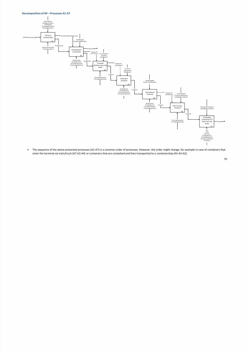
7/23/2019 Thesis Robert Heij Final Digital Version
http://slidepdf.com/reader/full/thesis-robert-heij-final-digital-version 70/94
70
Decomposition of A0 – Processes A1-A7
A1
Arrival of
containership
A2
(Un)loading of
container(s)
A3
Transport
between quay and
stacks
A4
Stacking of
container
A6
Inter-terminal
transport
A7
(Un)loading
container(s) on/
from train and
trucks
Handling plan
Container specifications
Quay crane(s)
Crane operator(s)Terminal transporters
(Transporter operators)
Captain containership
Transport company
Terminal transporter
(Transporter operator)
Containership
Container(s)
Container
Container
Containership
Arrival scheme
Vessel specifications
Handling plan
Terminal specifications
Berthing procedure
Containership
Container specifications
Loading plan truck/train
Container
specifications
Stacking plan
Terminal layout
Container
specifications
Container
Terminal layout
Container specifications
Loading plan truck/train
Activation signal to quay cranes
A5
Unstacking of
container
Container
Unstacking plan
Container specifications
Stacking crane
(Crane operator)
Terminal transporter
(Transporter operator)
Stacking crane
(Crane operator)
Terminal transporter
(Transporter operator)
Container
Terminal transporter
(Transporter operator)
Request for
terminal trucks
Request for
stacking crane
Request for
terminal truck
Train
Truck
Rail crane
(Crane operator)
Terminal transporter
(Transporter operator)
Truck driver
The sequence of the above presented processes (A1-A7) is a common order of processes. However, the order might change, for example in case of containers that
enter the terminal via train/truck (A7-A3-A4) or containers that are unstacked and then transported to a containership (A5-A3-A2).

7/23/2019 Thesis Robert Heij Final Digital Version
http://slidepdf.com/reader/full/thesis-robert-heij-final-digital-version 71/94
71
Decomposition of A1 – Berthing process
A1-2
Requesting berth
place
A1-3
Assigning quay
position
A1-4
Arriving and
mooring at
terminal
Berthing request
Berthing location
Assigned quay crane(s)
Arrival time
Captain
containership
Terminal
operator
Vessel specifications
Handling plan
Terminal specifications
Captain
containership
Activation signal to assigned quay crane(s)
A1-1
Navigating to portContainership
Containership
Containership
Captain
containership
Berthing
procedure
Containership
Arrival scheme
Terminal specifications:
- Quay length
- Number of quay cranes
- Availability of quay cranes
- Availability of quay length
Vessel specifications:
- Length of containership
- Number of quay cranes needed
- Expected arrival and departure

7/23/2019 Thesis Robert Heij Final Digital Version
http://slidepdf.com/reader/full/thesis-robert-heij-final-digital-version 72/94
72
Decomposition of A2 – (Un)loading of containers at quay side
A2-1
Activating quay
crane(s)
Activation signal
Activation
procedure
A2-2
Unloading of
containers
A2-3
Loading of
containers
A2-4
Deactivating quay
crane(s)
Containership
Quay crane(s)
Crane operator(s)
Unloading signal
Handling plan
Container specifications
Containership
Containershp
Deactivation signal
to quay cranes
Handling plan
Container
specifications
Loading signal
Quay crane(s)
Crane operator(s)
Terminal transporters
(Transporter operators)
Quay crane(s)
Crane operator(s)
Terminal transporters
(Transporter operators)
Quay crane(s)
Crane operator(s)
Container specifications:
- Position container (categorised into sections for assigning the quay cranes)
- Type of container (20ft/40 ft, normal/reefer, loaded/unloaded)
- Weight
Handling plan:
- Which containers need to be unloaded from and loaded onto the ship?
- Number and (un)loading order of containers (and origin-destination)

7/23/2019 Thesis Robert Heij Final Digital Version
http://slidepdf.com/reader/full/thesis-robert-heij-final-digital-version 73/94
73
Decomposition of A3 & A4 – Transport to stacking area and stacking of containers
Container
A4-2
Connecting
stacking crane to
container
A4-3
Transport container
to stack
A4-4
Placing container
on stack
A3-1
Transporter
moving to quay
crane
Terminal transporter
(Transporter operator)
Terminal truck
request
Quay crane
location
Container
specifications
Container
specifications
Releasing stacking crane
Container
Container
Container
A3-2 (A2-2-8)
Positioning of
container on
transporter
A3-3
Transport
between quay and
stacking area
Container
Container
Stacking crane
(Crane operator)
Terminal transporter
(Transporter operator)
Terminal transporter
(Transporter operator)
Terminal transporter
(Transporter operator)
Stacking crane
(Crane operator)
Terminal transporter
(Transporter operator)
Stacking crane
(Crane operator)
A4-1
Transporting
stacking crane to
transporter Unloading signal
Releasing terminal transporter
Seizing stacking crane
Stacking plan

7/23/2019 Thesis Robert Heij Final Digital Version
http://slidepdf.com/reader/full/thesis-robert-heij-final-digital-version 74/94
74
Decomposition of A5 & A6 – Unstacking of containers and transport to trains/trucks
A5-2
Connecting
stacking crane to
container
A5-3
Transport container
to terminal
transporter
A5-4
Placing container
on terminal
transporter
A6-2
Transport from
stacking area toquay or rail/truck
Stacking crane
(Crane operator)
Terminal transporter
(Transporter operator)
Terminal transporter
(Transporter operator)
A5-1
Transporting
stacking crane to
container
Container
Container
Request for terminal truck
Stacking crane
(Crane operator)
Stacking crane
(Crane operator)
Container
Stacking crane
(Crane operator)
Terminal transporter
(Transporter operator)
Container
Releasing stacking crane
Seizing stacking crane
Unstacking plan
Container
A6-1
Transporter
moving to stacking
crane Loading signal
Terminal transporter
(Transporter operator)
Terminal layout
The A5 process (unstacking container) and A6 process (requesting terminal equipment and transporting the container) intermingle.
The exact sequence of processes is dependent on t he type of equipment that is used. This process scheme represents the most common us ed process.

7/23/2019 Thesis Robert Heij Final Digital Version
http://slidepdf.com/reader/full/thesis-robert-heij-final-digital-version 75/94
75
Decomposition of A7 – (Un)loading containers on and from trains/trucks
(A7-1)
Moving
equipment to
container
(A7-2)
Connecting
equipment to
container
A7-3
Moving container
to truck / stack on
train
A7-4
Positioning
container on
truck/train
Container
Container
Container
Container
specifications
A7-5
Disconnecting
equipment from
container
Rail crane
(Crane operator)
Rail crane
(Crane operator)
Terminal transporter
(Transporter operator)
Train
Truck
Rail crane
(Crane operator)
Container
Rail crane
(Crane operator)
Loading plan
truck/train
Container
Train
Truck
Rail crane
(Crane operator)
(Terminal transporter)
(Transporter operator)
The A7-1 and A7-2 processes are dependent on the type of equipment that is used. In the following cases these two processes are not executed:
Trucks: the containers are often positioned on the truck with the same equipment as used for transport to the truck (same for unloading)
Trains: when the containers are positioned on the train with a reach stacker and this reach stacker is also used for transport from the stacking area to the train

7/23/2019 Thesis Robert Heij Final Digital Version
http://slidepdf.com/reader/full/thesis-robert-heij-final-digital-version 76/94
76
Appendix B: List of required data for consumption model
This appendix gives a detailed list of the data that is needed for the application of the energy consumption model
that is described in chapter 3. The data is explained in general in paragraph 3.2.
The general data that is needed concerns:- terminal layout specifications (i.e. number of quay cranes);
- arrival scheme containerships;
- number of containers to be handled;
- container load specifications;
- position of containers;
- energy consumption specifications (kW/s).
Terminal equipment
Terminal layout configuration
Quay cranes / rail cranes
o Type and number of quay cranes (and barge cranes)o Number of moves per crane
o Energy consumption idle state (kW/s)
o Energy consumption busy state (kW/s)
Horizontal movement of spreader
Hoisting the spreader
Lowering the spreader
Movement of quay crane on quay
o Auxiliary energy specifications (e.g. lighting, steer cabin)
o Layout specifications of terminal (to determine distances)
Terminal transporters
o Type and number of transporters
o Number of moves per transporter
o Energy consumption idle state (kW/s)
o Energy consumption busy state (kW/s)
Movement of transporter over terminal
(Hoisting spreader/container)
(Lowering spreader/container)
o Auxiliary energy specifications (e.g. lighting, steer cabin)
o Layout specifications of terminal (to determine distances)
Stacking cranes
o Type and number of stacking cranes
o Number of moves per stacking crane
o
Energy consumption idle state (kW/s)o Energy consumption busy state (kW/s)
Movement of crane over terminal
Horizontal movement of spreader
Hoisting spreader
Lowering spreader
o Auxiliary energy specifications (e.g. lighting, steer cabin)
o Layout specifications of terminal (to determine distances)
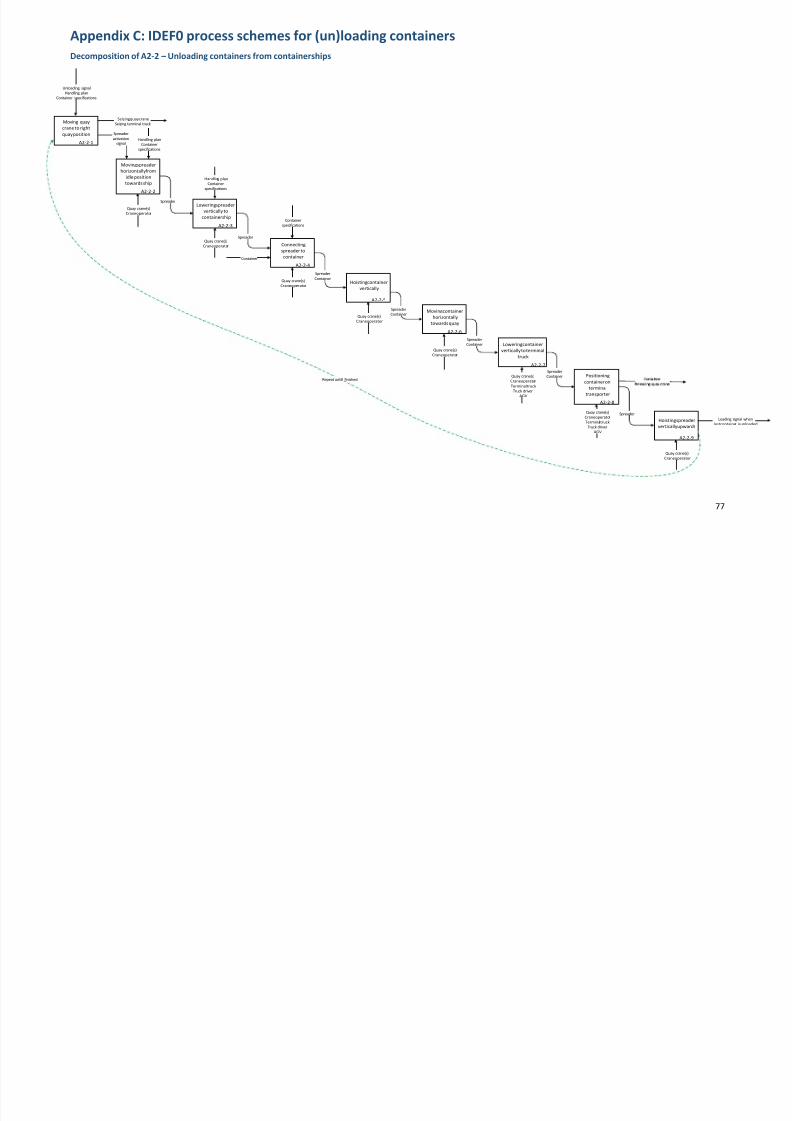
7/23/2019 Thesis Robert Heij Final Digital Version
http://slidepdf.com/reader/full/thesis-robert-heij-final-digital-version 77/94
77
Appendix C: IDEF0 process schemes for (un)loading containers
Decomposition of A2-2 – Unloading containers from containerships
A2-2-2
Moving spreader
horizontally from
idle position
towards ship
A2-2-3
Lowering spreader
vertically to
containership
A2-2-4
Connecting
spreader to
container
A2-2-5
Hoisting container
vertically
Quay crane(s)
Craneoperator
Quay crane(s)
Craneoperator
Quay crane(s)
Craneoperator
Quay crane(s)
Craneoperator
A2-2-6
Moving container
horizontally
towards quay
A2-2-7
Lowering container
vertically to terminal
truck
A2-2-8
Positioning
container on
terminal
transporter
A2-2-9
Hoisting spreader
vertically upwards
A2-2-1
Moving quay
crane to right
quay position
Repeat untill finished
Loading signal when
lastcontainer isunloaded
Unloading signal
Handling plan
Container specifications
Handling plan
Container
specifications
Handling plan
Container
specifications
Seizingquaycrane
Seizing terminal truck
Quay crane(s)
Craneoperator
Quay crane(s)
Craneoperator
Terminaltruck
Truck driverAGV
Quay crane(s)
Craneoperator
Terminaltruck
Truck driver
AGV
Quay crane(s)
Craneoperator
Container
specifications
Spreader
activationsignal
Spreader
Spreader
Spreader
Container
Container
Spreader
Container
Spreader
Container
Spreader
Container
Spreader

7/23/2019 Thesis Robert Heij Final Digital Version
http://slidepdf.com/reader/full/thesis-robert-heij-final-digital-version 78/94
78
Decomposition of A2-3 – Loading containers onto containerships
A2-3-5
Moving container
horizontally
towards ship
A2-3-6
Lowering
container
vertically to
containership
A2-3-3
Connecting
spreader to
container
A2-3-4
Hoisting container
vertically
Quay crane(s)
Craneoperator
Terminaltruck
Truck driver
AGV
Quay crane(s)Craneoperator
Terminaltruck
Truck driverAGV
Quay crane(s)Craneoperator
Quay crane(s)
Craneoperator
A2-3-9
Moving spreader
horizontally
towards quay
A2-3-2
Lowering spreader
vertically to
terminal truck
A2-3-7
Disconnecting
spreader from
container
A2-3-8
Hoisting spreadervertically upwards
A2-3-1
Moving quay
crane to right
quay position
Repeat untill finished
Loadingsignal
HandlingplanContainer
specifications
Handling plan
Container
specifications
Releasing quay crane
Spreaderactivationsignal
Spreader
Spreaderwith
container
Spreaderwith
container
Spreaderwith
container
Spreaderwithcontainer
Spreader
Spreader
Seizingquay crane
Container
Container
Signal to terminalwhenlastcontainer isloaded
Quay crane(s)
Craneoperator
Quay crane(s)
Craneoperator
Quay crane(s)
Craneoperator
Quay crane(s)Craneoperator
Terminaltruck
Truck driverAGV
Quay crane(s)
Craneoperator
Terminal truckTruck driver
Container
specifications
Handling plan
Container
specifications
Terminaltruck release signal

7/23/2019 Thesis Robert Heij Final Digital Version
http://slidepdf.com/reader/full/thesis-robert-heij-final-digital-version 79/94
79
Appendix D: Arrival scheme containerships
The arrival scheme that is used for simulating the MSCTV is shown in Table 18. Here an overview of the number
of containerships and corresponding number of containers (expressed in TEU and 40ft equivalents) can be found.
Table 18: Arrival scheme with number of containers per containership
Number
containership Start operations
Number
of TEU
Number of
(40ft.)
containers
1 1/12/2012 08:18:28 322 161
2 1/12/2012 08:45:12 585 293
3 1/12/2012 22:11:28 966 483
4 2/12/2012 02:20:48 666 333
5 2/12/2012 20:19:07 3805 1903
6 3/12/2012 14:15:57 1869 935
7 4/12/2012 02:26:32 641 3218 4/12/2012 14:23:14 1547 774
9 4/12/2012 20:17:01 1026 513
10 5/12/2012 08:22:03 532 266
11 5/12/2012 08:54:47 1068 534
12 5/12/2012 14:18:04 618 309
13 6/12/2012 01:29:30 696 348
14 6/12/2012 08:09:58 1716 858
15 6/12/2012 14:21:55 348 174
16 6/12/2012 20:17:37 737 369
17 6/12/2012 23:35:59 303 152
18 7/12/2012 05:25:15 1420 710
19 7/12/2012 19:36:23 1241 621
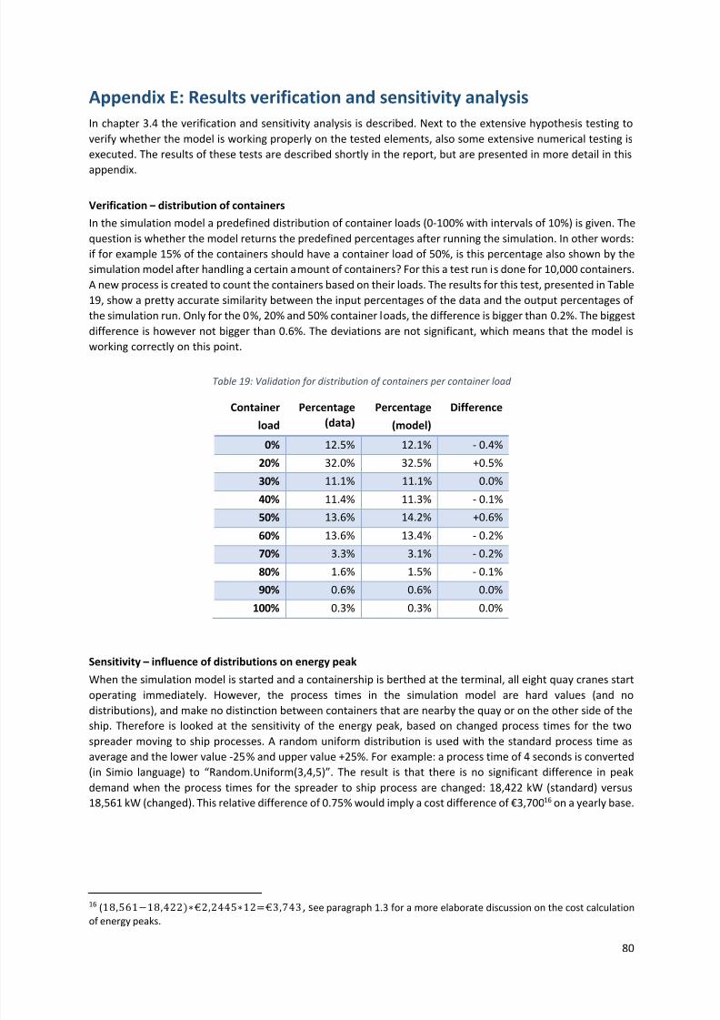
7/23/2019 Thesis Robert Heij Final Digital Version
http://slidepdf.com/reader/full/thesis-robert-heij-final-digital-version 80/94
80
Appendix E: Results verification and sensitivity analysis
In chapter 3.4 the verification and sensitivity analysis is described. Next to the extensive hypothesis testing to
verify whether the model is working properly on the tested elements, also some extensive numerical testing is
executed. The results of these tests are described shortly in the report, but are presented in more detail in this
appendix.
Verification – distribution of containers
In the simulation model a predefined distribution of container loads (0-100% with intervals of 10%) is given. The
question is whether the model returns the predefined percentages after running the simulation. In other words:
if for example 15% of the containers should have a container load of 50%, is this percentage also shown by the
simulation model after handling a certain amount of containers? For this a test run is done for 10,000 containers.
A new process is created to count the containers based on their loads. The results for this test, presented in Table
19, show a pretty accurate similarity between the input percentages of the data and the output percentages of
the simulation run. Only for the 0%, 20% and 50% container loads, the difference is bigger than 0.2%. The biggest
difference is however not bigger than 0.6%. The deviations are not significant, which means that the model is
working correctly on this point.
Table 19: Validation for distribution of containers per container load
Container
load
Percentage
(data)
Percentage
(model)
Difference
0% 12.5% 12.1% - 0.4%
20% 32.0% 32.5% +0.5%
30% 11.1% 11.1% 0.0%
40% 11.4% 11.3% - 0.1%
50% 13.6% 14.2% +0.6%
60% 13.6% 13.4% - 0.2%70% 3.3% 3.1% - 0.2%
80% 1.6% 1.5% - 0.1%
90% 0.6% 0.6% 0.0%
100% 0.3% 0.3% 0.0%
Sensitivity – influence of distributions on energy peak
When the simulation model is started and a containership is berthed at the terminal, all eight quay cranes start
operating immediately. However, the process times in the simulation model are hard values (and no
distributions), and make no distinction between containers that are nearby the quay or on the other side of theship. Therefore is looked at the sensitivity of the energy peak, based on changed process times for the two
spreader moving to ship processes. A random uniform distribution is used with the standard process time as
average and the lower value -25% and upper value +25%. For example: a process time of 4 seconds is converted
(in Simio language) to “Random.Uniform(3,4,5)”. The result is that there is no significant difference in peak
demand when the process times for the spreader to ship process are changed: 18,422 kW (standard) versus
18,561 kW (changed). This relative difference of 0.75% would imply a cost difference of €3,70016 on a yearly base.
16 (18,561−18,422∗€2,2445∗12€3,743, see paragraph 1.3 for a more elaborate discussion on the cost calculation
of energy peaks.

7/23/2019 Thesis Robert Heij Final Digital Version
http://slidepdf.com/reader/full/thesis-robert-heij-final-digital-version 81/94
81
Appendix F: Results simulation model
Table 20: Detailed results for limiting number of simultaneously lifting quay cranes at 8-crane terminal
Number
of quay
cranes
Number of
lifting quay
cranes
PeakDem
and
Half width
peak
demand
Peak
reduction
(%)
PeakCosts
(€/year)
Total
savings
(€/year)
Handling time
(hours/week)
Handling
time
(hours/year)
Extra
handlin
g time
Extra handling
time
(sec/year)
Total savings
per second
(€/sec.)
Delayed
containers
(%)
average waiting
time
(sec./container)
8 8 19230 467.6 - € 517,941 - 30.9 2460.0 - - - 0.0% 0.0
8 7 17828 362.0 7.3% € 480,166 € 37,775 31.0 2462.0 0.08% 7,315 € 5.16 0.2% 7.2
8 6 15598 514.1 18.9% € 420,123 € 97,818 31.0 2464.3 0.18% 15,672 € 6.24 0.6% 5.4
8 5 13651 424.0 29.0% € 367,676 € 150,265 31.0 2466.7 0.27% 24,305 € 6.18 1.6% 3.9
8 4 11988 302.0 37.7% € 322,878 € 195,063 31.0 2469.1 0.37% 32,938 € 5.92 5.7% 2.9
8 3 9239 218.1 52.0% € 248,847 € 269,094 31.3 2488.7 1.17% 103,446 € 2.60 17.8% 2.9
8 2 6689 114.7 65.2% € 180,168 € 337,773 32.7 2604.4 5.87% 520,095 € 0.65 59.4% 4.4
8 1 4102 27.1 78.7% € 110,480 € 407,461 57.3 4561.6 85.43% 7,565,969 € 0.05 99.8% 37.6
Table 21: Detailed results for limiting number of simultaneously lifting quay cranes at 6-crane terminal
Number
of quay
cranes
Number of
lifting quay
cranes
PeakDem
and
Half width
peak
demand
Peak
reduction
(%)
PeakCosts
(€/year)
Total
savings
(€/year)
Handling time
(hours/week)
Handling
time
(hours/year)
Extra
handlin
g time
Extra handling
time
(sec/year)
Total savings
per second
(€/sec.)
Delayed
containers
(%)
average waiting
time
(sec./container)
6 6 14940 312,3 - € 402.397 - 41,2 3277,4 - - - 0,0% 0,0
6 5 13280 296,5 11,1% € 357.687 € 44.710 41,2 3278,2 0,03% 3049 € 14,67 0,3% 5,5
6 4 11134 165,1 25,5% € 299.883 € 102.514 41,2 3279,6 0,07% 7839 € 13,08 1,7% 3,4
6 3 9187 162,7 38,5% € 247.436 € 154.961 41,4 3291,9 0,44% 52289 € 2,96 7,2% 2,8
6 2 6552 12,4 56,1% € 176.475 € 225.922 42,1 3349,1 2,19% 258119 € 0,88 29,9% 3,3
6 1 3811 33,5 74,5% € 102.639 € 299.759 57,4 4565,6 39,30% 4637439 € 0,06 99,7% 17,0

7/23/2019 Thesis Robert Heij Final Digital Version
http://slidepdf.com/reader/full/thesis-robert-heij-final-digital-version 82/94
82
Table 22: Detailed results for limiting maximum energy demand at 8-crane terminal
Number of
quay
cranes
Maximum
energy
demand
(kW)
PeakDema
nd
Half width
peak
demand
Peak
reduction
(%)
PeakCosts
(€/year)
Total savings
(€/year)
Handling
time
(hours/week)
Handling
time
(hours/yr)
Extra
handling
time
Extra
handling
time
(sec/year)
Total savings
per second
(€/sec.)
Delayed
containers
(%)
average waiting
time
(sec./container)
8 Infinity 19,230 467.6 - € 517,941 - 30.9 2461.3 - - - 0.0% 0.0
8 20,000 19,195 427.2 -0.2% € 517,008 € 933 30.9 2461.3 0.0% 48 € 19.54 0.0% 0.1
8 19,000 18,788 267.9 -2.3% € 506,043 € 11,898 30.9 2461.1 0.0% -573 -€ 20.77 0.0% 1.4
8 18,000 17,907 69.7 -6.9% € 482,311 € 35,630 30.9 2461.1 0.0% -620 -€ 57.43 0.1% 2.1
8 17,000 16,954 33.3 -11.8% € 456,646 € 61,295 30.9 2459.8 -0.1% -5,393 -€ 11.37 0.1% 2.7
8 16,000 15,972 13.8 -16.9% € 430,190 € 87,751 30.9 2461.6 0.0% 1,432 € 61.29 0.3% 3.2
8 15,000 14,983 14.7 -22.1% € 403,542 € 114,399 31.0 2462.8 0.1% 5,727 € 19.97 0.4% 3.6
8 14,000 13,991 7.5 -27.2% € 376,830 € 141,111 30.9 2461.1 0.0% -716 -€ 197.10 0.5% 3.9
8 13,000 12,990 6.3 -32.4% € 349,869 € 168,072 30.9 2461.4 0.0% 668 € 251.53 0.9% 4.0
8 12,000 11,994 5.8 -37.6% € 323,053 € 194,888 31.0 2463.2 0.1% 7,105 € 27.43 1.4% 3.7
8 11,000 10,993 6.7 -42.8% € 296,072 € 221,869 31.0 2462.5 0.1% 4,534 € 48.93 2.3% 3.6
8 10,000 9,997 3.4 -48.0% € 269,256 € 248,685 31.0 2464.7 0.1% 12,362 € 20.12 3.7% 3.5
8 9,000 8,999 1.1 -53.2% € 242,376 € 275,565 31.0 2468.6 0.3% 26,584 € 10.37 6.9% 3.4
8 8,000 7,999 0.8 -58.4% € 215,445 € 302,496 31.1 2474.8 0.5% 48,635 € 6.22 11.4% 3.6
8 7,000 6,999 1.2 -63.6% € 188,511 € 329,430 31.3 2492.8 1.3% 113,402 € 2.90 20.0% 3.8
8 6,000 5,999 0.9 -68.8% € 161,584 € 356,357 31.9 2541.2 3.2% 287,800 € 1.24 38.6% 5.1
8 5,000 4,999 0.4 -74.0% € 134,650 € 383,291 35.0 2787.4 13.3% 1,174,108 € 0.33 70.8% 9.0
8 4,000 4,000 0.0 -79.2% € 107,736 € 410,205 44.7 3558.8 44.6% 3,951,111 € 0.10 91.6% 22.0
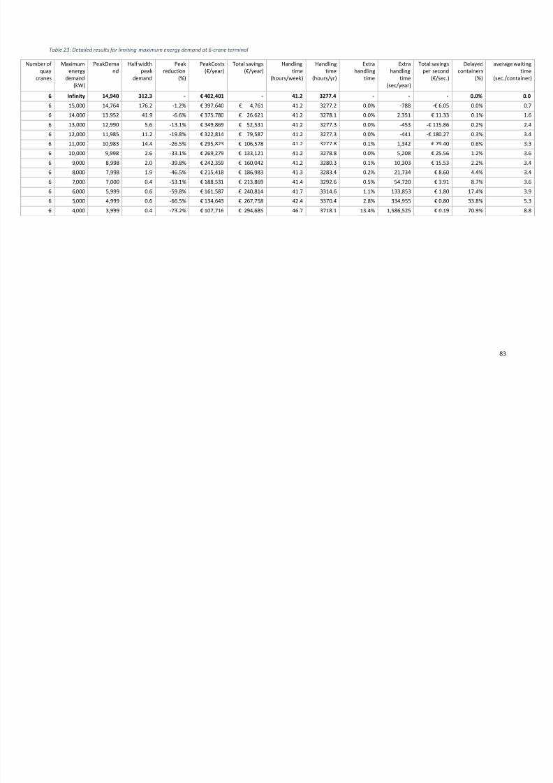
7/23/2019 Thesis Robert Heij Final Digital Version
http://slidepdf.com/reader/full/thesis-robert-heij-final-digital-version 83/94
83
Table 23: Detailed results for limiting maximum energy demand at 6-crane terminal
Number of
quay
cranes
Maximum
energy
demand
(kW)
PeakDema
nd
Half width
peak
demand
Peak
reduction
(%)
PeakCosts
(€/year)
Total savings
(€/year)
Handling
time
(hours/week)
Handling
time
(hours/yr)
Extra
handling
time
Extra
handling
time
(sec/year)
Total savings
per second
(€/sec.)
Delayed
containers
(%)
average waiting
time
(sec./container)
6 Infinity 14,940 312.3 - € 402,401 - 41.2 3277.4 - - - 0.0% 0.0
6 15,000 14,764 176.2 -1.2% € 397,640 € 4,761 41.2 3277.2 0.0% -788 -€ 6.05 0.0% 0.7
6 14,000 13,952 41.9 -6.6% € 375,780 € 26,621 41.2 3278.1 0.0% 2,351 € 11.33 0.1% 1.6
6 13,000 12,990 5.6 -13.1% € 349,869 € 52,531 41.2 3277.3 0.0% -453 -€ 115.86 0.2% 2.4
6 12,000 11,985 11.2 -19.8% € 322,814 € 79,587 41.2 3277.3 0.0% -441 -€ 180.27 0.3% 3.46 11,000 10,983 14.4 -26.5% € 295,823 € 106,578 41.2 3277.8 0.1% 1,342 € 79.40 0.6% 3.3
6 10,000 9,998 2.6 -33.1% € 269,279 € 133,121 41.2 3278.8 0.0% 5,208 € 25.56 1.2% 3.6
6 9,000 8,998 2.0 -39.8% € 242,359 € 160,042 41.2 3280.3 0.1% 10,303 € 15.53 2.2% 3.4
6 8,000 7,998 1.9 -46.5% € 215,418 € 186,983 41.3 3283.4 0.2% 21,734 € 8.60 4.4% 3.4
6 7,000 7,000 0.4 -53.1% € 188,531 € 213,869 41.4 3292.6 0.5% 54,720 € 3.91 8.7% 3.6
6 6,000 5,999 0.6 -59.8% € 161,587 € 240,814 41.7 3314.6 1.1% 133,853 € 1.80 17.4% 3.9
6 5,000 4,999 0.6 -66.5% € 134,643 € 267,758 42.4 3370.4 2.8% 334,955 € 0.80 33.8% 5.3
6 4,000 3,999 0.4 -73.2% € 107,716 € 294,685 46.7 3718.1 13.4% 1,586,525 € 0.19 70.9% 8.8

7/23/2019 Thesis Robert Heij Final Digital Version
http://slidepdf.com/reader/full/thesis-robert-heij-final-digital-version 84/94
84
Appendix G: Paper
On the next pages, the paper can be found that is written as part of the master thesis project. The paper is
proposed to be published in Transport Policy, ‘an international refereed journal aimed at bridging the gap
between theory and practice in transport’ (Elsevier, 2015). For this purpose the lay-out of the paper is adapted
to the standards of Transport Policy.
7/23/2019 Thesis Robert Heij Final Digital Version
http://slidepdf.com/reader/full/thesis-robert-heij-final-digital-version 85/94
85
Transport Policy
Opportunities for peak shaving energy demand of ship to
shore quay cranes at container terminals
Robert Heij
Delft University of Technology, Faculty of Technology, Policy and Management
----------------------------------------------------------------------------------------------------------------------------------------------------------------------
Abstract
This paper presents the results of both a qualitative and quantitative study towards the possibilities for peak shaving the
energy demand of ship-to-shore cranes at container terminals. The objective of this paper is to present an energy consumption
model that visualises the energy demand of ship-to-shore cranes and to show the possibilities for reducing the peak demand
of ship-to-shore cranes by implementing rules of operation (i.e. changes to the business operational procedures). The results
show that the peak demand (and peak related costs) can be reduced by 50%, while the handling time of containerships
increases by less than half a minute per hour handling time. This can be achieved by reducing the maximum energy demand of
all operating ship-to-shore cranes or by limiting the maximum number of simultaneously lifting ship-to-shore cranes. By
implementing (one of) these rules of operation an intermediate container with 6-8 ship-to-shore (STS) cranes is able to save
up to €250,000 per year, which is about 48% of the total peak-related energy costs.
Keywords: Peak shaving; Container terminals; Electricity demand; Energy consumption; Ship-to-shore cranes
----------------------------------------------------------------------------------------------------------------------------------------------------------------------
1 Introduction
1.1
Growth in containerised transport
The worldwide throughput of containers is growing
continuously. The standardised size of the container (in
20ft. and 40ft. equivalents) makes it a suitable mean for
transporting all kinds of products, ranging from multimedia
and building material to clothing and shoes. Even
temperature-sensitive goods like flowers, fruits and
vegetables can be transported easily by temperature-
controlled containers, known as reefers. The share of
containerised transport in seaborne trade increased from
2.75% (1980) to 16.5% (2013), while the total seaborne
trade increased with 158% over this period (UNCTAD,
2013). The annual worldwide transport of containers
increased from 28.7 million TEU in 1990 to 153 million TEU
in 2010 (World Shipping Council, 2011). The 20-years
average growth percentage of the container market shows
a remarkable 7.8% (Clarksons, 2015).
An important development that facilitates the growing
container market is the growing capacities of
containerships. Where the largest containership in 1980
had a capacity of 3,000 TEU, the biggest containerships
operating in 2015 have a capacity of almost 19,224 TEU
(Lloyd's List, 2015).
The growing size of containerships influences the
container terminals’ operations, since the number ofcontainers per containership also increased due to this
development. Container carriers demand container
terminals to handle their ships as fast as possible to
continue their journey to the next port. This higher
productivity is achieved by more automated terminal
processes (Grunow, Günther, & Lehmann, 2005) and by
deploying more terminal equipment simultaneously.
However, with more and more simultaneously operating
ship-to-shore cranes, the energy demand (kW/s) is
increasing. This also increases the highest observed peak
demand, leading to a higher energy bill and therefore
higher handling costs.
The peak demand of container terminals is responsible
for about 25-30% of the monthly energy bill (ABB, 2014)
(Stedin, 2014). The main reason is that the highest
observed peak demand is charged for the next twelve
months. To illustrate this: if the highest peak in January is
12,000kW, the terminal is charged 12,000 times the
monthly tariff for the rest of the year. However, when the
highest peak in March is 14,000kW, the terminal is charged
14,000 times the monthly tariff until March the year after.
A lower peak demand might save container terminals at

7/23/2019 Thesis Robert Heij Final Digital Version
http://slidepdf.com/reader/full/thesis-robert-heij-final-digital-version 86/94
86
least tens of thousands euros per year. It is therefore very
important to investigate the possibilities to reduce this
peak demand.
The research objective is therefore to investigate the
possibilities for peak shaving the electricity demand at
container terminals by applying new rules of operation forelectricity consuming terminal processes, while meanwhile
monitoring the consequences for the handling speed of
containerships.
This paper presents the results of this research by
discussing the terminal operations and volatility of the
energy demand of STS cranes in chapter 1. The applied
methodology and relevance are presented in chapter 2.
Chapter 3 presents the energy consumption model, which
forms the basis for the developed simulation model. The
simulation model is presented in chapter 4 and the results
of the simulation study are discussed in chapter 5. The
implications of these results and conclusions of the study
are discussed in chapter 5 and 6.
1.2
Operations ship-to-shore cranes
After a containership has berthed at the sea-side of a
terminal, the ship-to-shore cranes start unloading the
incoming containers based on the unloading plan. Ship-to-
shore cranes can use a normal spreader, enabling them to
handle one container at a time or more advanced
spreaders (e.g. the twin-lift and tandem-lift) to handle
multiple containers at the same time (Stahlbock & Voß,
2008). The Super Post Panamax ship-to-shore cranes, thecurrent standard for unloading the largest containerships,
are able to make approximately 32 lifts per crane per hour
(APM Terminals, 2014). This allows a ship-to-shore crane to
handle 32-64 TEU per hour with a normal spreader and up
to 128 TEU per hour with a tandem lift spreader.
The handling capacity of a container terminal is highly
dependent on the number of ship-to-shore cranes and
their capacity, since the cranes determine the handling
time for a ship as well as the throughput of containers to
the stacking process (Eugen, Şerban, Augustin, & Ştefan,
2014).During the (un)loading of a containership, two criteria
are important: the ship’s stability and number of
unproductive moves (Imai, Sasaki, Nishimura, &
Papadimitriou, 2006). While (un)loading, the ship’s stability
changes due to the continuously changing container load.
Because containerships visit several container terminals,
each of them unloading containers from and loading
containers to the ship, not all containers which have to be
unloaded are positioned on top of the ship’s stacks. The
ships therefore have to be loaded in an efficient way,
allowing the next container terminal to unload the
containership with a minimum of unproductive moves.
These two criteria are often in conflict, because the most
efficient loading (regarding the minimisation of
unproductive moves) might not also be in line with the
most efficient loading regarding the ship’s stability. Thismakes the stowage very complex (Bortfeldt & Gehring,
2001) (Steenken, Voß, & Stahlbock, 2004) (Dekker, Voogd,
& Van Asperen, 2006), especially because the stowage
plans have to be aligned over all different ports that have
to (un)load the ship (Wilson & Roach, 2000).
1.3
Volatility of energy demand
The ship-to-shore cranes are connected to the electricity
network. For all quay crane processes (moving of crane and
spreader, crane lighting and auxiliary processes) electricity
is supplied by the netwerk. The vertical movements have
the most volatile energy demand, showing high peaks for
hoisting spreader of the crane and low falls for lowering the
spreader, as can be seen in Figure 1 (MSC Terminal
Valencia, 2009). The gantry (horizontal) movements and
auxiliary energy consumption show a less volatile
character.
Figure 1: Detailed energy consumption of quay crane (MSCTerminal Valencia, 2009)
In Figure 2 the total energy consumption for one ship-to-
shore crane is visualised. In total two peaks can be
identified for handling a container. The first peak for lifting
a spreader and container above the ship and the second
peak for lifting the spreader after the container is
positioned on the terminal. When all ship-to-shore cranes
on a terminal are lifting at the same moment, the potential
peak demand is very high. This supports the importance of
the first paragraph to visualise the peak demand of a
-600,00
-400,00
-200,00
0,00
200,00
400,00
600,00
800,00
1.000,00
3 - 1 2 - 2 0 0 9 1 6 : 2 4
3 - 1 2 - 2 0 0 9 1 6 : 2 5
3 - 1 2 - 2 0 0 9 1 6 : 2 6
3 - 1 2 - 2 0 0 9 1 6 : 2 7
3 - 1 2 - 2 0 0 9 1 6 : 2 8
3 - 1 2 - 2 0 0 9 1 6 : 2 9
3 - 1 2 - 2 0 0 9 1 6 : 3 0
3 - 1 2 - 2 0 0 9 1 6 : 3 1
3 - 1 2 - 2 0 0 9 1 6 : 3 2
E n e r g y c o n s u m p t i o n s h i p - t o - s h o r e c r a n e ( k W )
Time
Total (kW)
Vertical movement spreader (kW)
Gantry (kW)
Auxiliary consumption (kW)

7/23/2019 Thesis Robert Heij Final Digital Version
http://slidepdf.com/reader/full/thesis-robert-heij-final-digital-version 87/94
87
terminal while handling a containership and to investigate
the opportunities to reduce the peak demand.
Figure 2: Energy consumption for handling one container (ABB,
2014)
1.4
Challenge for container terminals
The growing need for container terminals to handle
containerships as fast as possible leads to more
automatisation and more simultaneously operating ship-
to-shore cranes, leading to high peaks in electricity
demand. Because an observed peak demand is charged for
the next twelve months, the highest peak is responsible for
nearly 25-30% of the total electricity costs. This implies that
higher handling speeds of containerships result in more
peak related energy costs, leading to higher handling costs.
Because container carriers request both higher handling
speeds and lower handling costs, terminals are confronted
with a dilemma. The challenge is therefore to find
opportunities to reduce the peak related costs without
reducing the handling speed too much.
2 Research and methodology
2.1
Research objective
The objective of the research is to investigate the
opportunities for peak shaving the electricity demand,
while monitoring the consequences for the handling speed
of containerships. Peak shaving implies the lowering of the
highest observed peak in energy demand to reduce the
energy related costs. This enables container terminals to
lower the handling costs of containerships, giving them a
better competitive position. Another advantage of peak
shaving is that the energy demand of terminals is more
stable, which is especially important for container
terminals in countries where grid operators cannot
prepare the energy system for unexpected high energy
peaks. The handling time for containerships needs to be
monitored, because extra handling time might affect the
terminals’ competitive position. The main research
question that is addressed in this research is:
“What are the possibilities for reducing the peak demand
of electricity consuming terminal equipment (peak shaving)
in order to reduce the electricity related energy costs?”
The hypothesis is that by implementing different rules of
operation (i.e. process improvements), like limiting the
number of lifting cranes of the maximum allowed energydemand, terminals are able to reduce the height of peaks,
which reduces the energy-related costs.
2.2
Relevance
2.2.1
Scientific relevance
Previous research towards the energy consumption of
container terminals (Geerlings & Van Duin, 2011) (Van der
Voet, 2008) does not provide in visualising the peak
demand of container terminals or ship-to-shore cranes.
The research has two contributions to science.
1. The first scientific contribution is to develop an
energy consumption model that is able to show the
energy demand over time (in kW/s). Over the last
years many studies have been executed towards the
energy efficiency of container terminals. The models
that are presented in these studies try to describe the
total energy consumption over a given time interval
(mostly in kWh per year). However, for visualising the
peak demand of container terminals, and in particular
the ship-to-shore cranes, a more advanced model
needs to be developed. This consumption model can
also be applied to visualise the energy demand of
other types of cranes in different industries.2. The second contribution is to present rules of
operation that contribute to the reduction of peak
demand at container terminals and to test these rules
of operation by executing a case-study to show the
opportunities for peak shaving the energy demand of
ship-to-shore cranes.
2.2.2
Business relevance
The growth of containerships is increasing continuously,
into the newest generation which is able to carry almost
20,000 TEU. Container terminals feel a high pressure tohandle ships as fast as possible against a low price, to
improve their competitive position. However, when more
and more ship-to-shore cranes are simultaneously
executing a lifting movement, the peak demand and
energy-related costs increase. For an intermediate
container terminal with eight ship-to-shore quay cranes,
the peak related costs can count up to 20-30% of the total
energy costs. The energy consumption model and
developed rules of operation show the opportunities for
container terminals to reduce these peak related costs,
while monitoring the consequences for the handling time.
-2000
-1000
0
1000
2000
3000
E N E R G Y D E M A N
D ( K W )
TIME

7/23/2019 Thesis Robert Heij Final Digital Version
http://slidepdf.com/reader/full/thesis-robert-heij-final-digital-version 88/94
88
This can save a terminals at least tens of thousands euros
per year.
2.3
Methodology
The research is executed in three different parts:
1.
At first an extensive literature review is executedtowards the container market and in particular the
ship-to-shore crane operations. This leads to a
better understanding of the problem and shows the
importance to reduce the peak demand of ship-to-
shore cranes;
2.
Based on the acquainted knowledge an energy
consumption model is developed by introducing a
conceptual model and a final consumption model
(mathematical formula).
3.
The conceptual model is applied for a container
terminal, so rules of operation can be tested
quantitatively on their ability to reduce the peak
demand. The simulation model is developed in a
discrete-event environment, with the Simio
software package (Simio LLC, 2015). The discrete
modelling approach enables the modeller to model
the containers as passive objects with a predefined
behaviour and to visualise the energy demand per
second, as time is continuing based on the
occurrence of events. Other environments, like
system dynamics or agent-based modelling do not
facilitate in all of these aspects.
The discrete environment has been applied inearlier research, for example to model the rail
operations (Caballini, Pasquale, Sacone, & Siri,
2014), the time duration of handling activities
(Cartenì & De Luca, 2011), to model and test several
container stacking algorithms (Van Asperen,
Borgman, & Dekker, 2010) and to model the
container flows within container terminals
(Alessandri, Cervellera, Cuneo, Gaggero, & Soncin,
2008) (Alessandri, Sacone, & Siri, 2007).
3
Energy consumption model
3.1 Conceptual model
As discussed earlier, the energy consumption of ship-to-
shore cranes is highly dependent on the different
movements that are made by the crane. In total six
different general movements can be distinguished:
1.
Moving spreader from quay to ship;
2. Lowering spreader at ship side;
3.
Hoisting spreader at ship side;
4.
Gantry (i.e. horizontal) movement from ship to
shore;
5.
Lowering spreader at quay side;
6. Hoisting spreader at quay side.
Each of these movements has its own energy
consumption specifications (see Figure 1 and Figure 2 in
§1.3). Next to these different movements, the auxiliary
energy consumption is also important to include. Theauxiliary consumption is a fixed energy demand per hour,
needed for keeping the pressure on the crane and for
equipment in the cabin and engine room. The auxiliary
consumption is rather constant over time because the
quay cranes are not turned off while in idle or off-shift
state.
The conceptual model, visualised in Figure 3, is built on
the idea of different energy specifications per type of
movement and state (since the auxiliary energy
consumption is also consumed in idle state). For all ship-to-
shore cranes need to be determined at which moment in
time a movement is executed. In that case the energy
consumption (kW/s) is added to the current energy
consumption. The auxiliary energy consumption per ship-
to-shore crane is multiplied with the number of cranes and
also added to the energy consumption, resulting in the
total energy consumption for all ship-to-shore cranes.
When doing this every second, the energy consumption
can be visualised over time enabling the identification of
peaks in energy demand.
For all types of movements
(1..n)
Energy consumption for
particular movement
(kW/s)
Energy consumption
equipment over time
(kW/s)
Auxiliary energy
consumption
(kW/s)
For all ship-to-shore cranes
(1..n)
Currently executing
movement?
(0/1)
Figure 3: Conceptual model for visualizing the energy demand
(kW/s)
3.2
Energy consumption model
The final energy consumption model is the mathematical
representation of the conceptual model that is presented
by Figure 3 in paragraph 3.1. As is shown in equation 01,
the energy consumption is obtained by multiplying – for
every ship-to-shore crane separately – the energy
consumption specifications for the movement that is
7/23/2019 Thesis Robert Heij Final Digital Version
http://slidepdf.com/reader/full/thesis-robert-heij-final-digital-version 89/94
89
currently executed and by adding the auxiliary energy
consumption.
Energy consumption container terminal per second
(equation 01):
∑(∑ ∗=4
=1) +
=4
=1
Where ℎ = type of terminal equipment
= number of all terminal equipment:
1= quay cranes, 2= (automated) stacking
cranes
3= rail cranes, 4= (barge cranes)
= type of movement
= number of all movements:
1= movement over terminal, 2= horizontalmovement of spreader, 3= hoisting
spreader, 4= lowering spreader
=
executing particular type of movement for
corresponding type of equipment? (binary: 0
if negative, 1 if positive)
= energy consumption for particular type of
movement, particular type of equipment
and container load (kW/s)
= auxiliary energy consumption for particular
type of terminal equipment
Where ℎ = type of terminal equipment
= number of all terminal equipment
= type of movement
= number of all movements
=
executing particular type of movement for
corresponding type of equipment? (binary: 0
if negative, 1 if positive)
= energy consumption for particular type of
movement, particular type of equipment
and container load (kW/s)
= auxiliary energy consumption for particular
type of equipment
When applying this energy consumption model over alonger period in time, the time aspect need to be added to
the formula. Equation 02 shows the mathematical
representation that can be used to visualise the energy
demand of ship-to-shore cranes over time.
Energy consumption container terminal per second for
(T-T0) (equation 02):
∫(∑(∑ ∗=4
=1) +
=4
=1)
=
Where 0 = starting time for measuring energy consumption
= final time for measuring energy consumption
The energy consumption model is not only suitable for
visualising the energy demand of ship-to-shore cranes, but
can also be used for other crane operations at container
terminals (e.g. Automated Stacking Cranes and rail cranes),but even in different type of industries where cranes are
used (e.g. factories or building sites).
4 Application of consumption model
4.1
Development of simulation model
As described in paragraph 2.3, a discrete-event
simulation model is constructed to apply the consumption
model that is presented in chapter 3. When a containership
arrives and is berthed, the terminal’s quay cranes are able
to start the handling of containers immediately. The quay
cranes take the containers through the earlier presented
six movements.
The model is able to generate the following relevant
output:
- energy consumption per second (kW/s);
-
handling time for containers (seconds);
-
number of active quay cranes;
-
number of lifting quay cranes;
- number of containers that were ceased and their
average ceasing time (due to limitations imposed by
the rules of operation).
In Figure 4 a 3D-view of the simulation model is given.Here eight quay cranes are transporting the containers (red
triangles) through the different (sub)movements. The
results of the simulation model are verified with real data
and by expert opinion (ABB, 2014).
Figure 4: Screen view of simulation model
4.2
Rules of operation
The rules of operation can that are implemented need to
be seen as process improvements to reduce the peak
demand for ship-to-shore cranes. In total two rules of
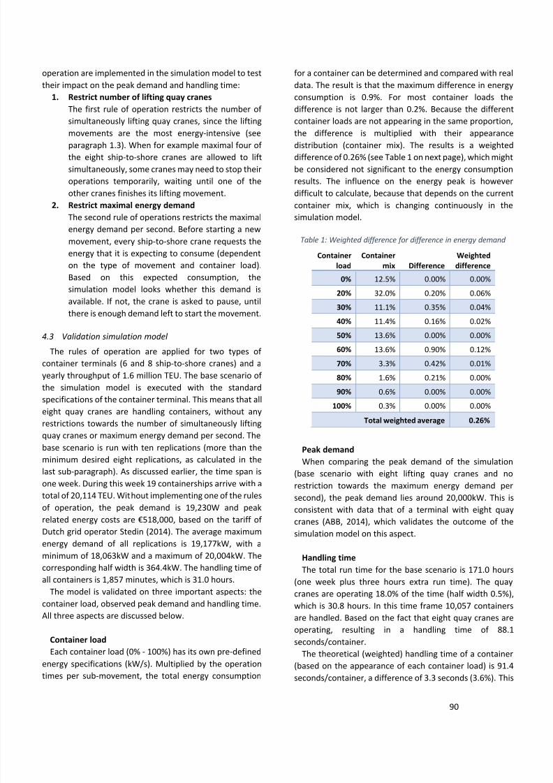
7/23/2019 Thesis Robert Heij Final Digital Version
http://slidepdf.com/reader/full/thesis-robert-heij-final-digital-version 90/94
90
operation are implemented in the simulation model to test
their impact on the peak demand and handling time:
1. Restrict number of lifting quay cranes
The first rule of operation restricts the number of
simultaneously lifting quay cranes, since the lifting
movements are the most energy-intensive (seeparagraph 1.3). When for example maximal four of
the eight ship-to-shore cranes are allowed to lift
simultaneously, some cranes may need to stop their
operations temporarily, waiting until one of the
other cranes finishes its lifting movement.
2. Restrict maximal energy demand
The second rule of operations restricts the maximal
energy demand per second. Before starting a new
movement, every ship-to-shore crane requests the
energy that it is expecting to consume (dependent
on the type of movement and container load).
Based on this expected consumption, the
simulation model looks whether this demand is
available. If not, the crane is asked to pause, until
there is enough demand left to start the movement.
4.3
Validation simulation model
The rules of operation are applied for two types of
container terminals (6 and 8 ship-to-shore cranes) and a
yearly throughput of 1.6 million TEU. The base scenario of
the simulation model is executed with the standard
specifications of the container terminal. This means that all
eight quay cranes are handling containers, without anyrestrictions towards the number of simultaneously lifting
quay cranes or maximum energy demand per second. The
base scenario is run with ten replications (more than the
minimum desired eight replications, as calculated in the
last sub-paragraph). As discussed earlier, the time span is
one week. During this week 19 containerships arrive with a
total of 20,114 TEU. Without implementing one of the rules
of operation, the peak demand is 19,230W and peak
related energy costs are €518,000, based on the tariff of
Dutch grid operator Stedin (2014). The average maximum
energy demand of all replications is 19,177kW, with a
minimum of 18,063kW and a maximum of 20,004kW. The
corresponding half width is 364.4kW. The handling time of
all containers is 1,857 minutes, which is 31.0 hours.
The model is validated on three important aspects: the
container load, observed peak demand and handling time.
All three aspects are discussed below.
Container load
Each container load (0% - 100%) has its own pre-defined
energy specifications (kW/s). Multiplied by the operation
times per sub-movement, the total energy consumption
for a container can be determined and compared with real
data. The result is that the maximum difference in energy
consumption is 0.9%. For most container loads the
difference is not larger than 0.2%. Because the different
container loads are not appearing in the same proportion,
the difference is multiplied with their appearancedistribution (container mix). The results is a weighted
difference of 0.26% (see Table 1 on next page), which might
be considered not significant to the energy consumption
results. The influence on the energy peak is however
difficult to calculate, because that depends on the current
container mix, which is changing continuously in the
simulation model.
Table 1: Weighted difference for difference in energy demand
Container
load
Container
mix Difference
Weighted
difference
0% 12.5% 0.00% 0.00%
20% 32.0% 0.20% 0.06%
30% 11.1% 0.35% 0.04%
40% 11.4% 0.16% 0.02%
50% 13.6% 0.00% 0.00%
60% 13.6% 0.90% 0.12%
70% 3.3% 0.42% 0.01%
80% 1.6% 0.21% 0.00%
90% 0.6% 0.00% 0.00%
100% 0.3% 0.00% 0.00%
Total weighted average 0.26%
Peak demand
When comparing the peak demand of the simulation
(base scenario with eight lifting quay cranes and no
restriction towards the maximum energy demand per
second), the peak demand lies around 20,000kW. This is
consistent with data that of a terminal with eight quay
cranes (ABB, 2014), which validates the outcome of the
simulation model on this aspect.
Handling time
The total run time for the base scenario is 171.0 hours
(one week plus three hours extra run time). The quay
cranes are operating 18.0% of the time (half width 0.5%),
which is 30.8 hours. In this time frame 10,057 containers
are handled. Based on the fact that eight quay cranes are
operating, resulting in a handling time of 88.1
seconds/container.
The theoretical (weighted) handling time of a container
(based on the appearance of each container load) is 91.4
seconds/container, a difference of 3.3 seconds (3.6%). This

7/23/2019 Thesis Robert Heij Final Digital Version
http://slidepdf.com/reader/full/thesis-robert-heij-final-digital-version 91/94
91
difference could be explained by random distribution of
process times for engaging the container in the simulation
model, while the theoretical handling time makes use of
standard process times instead of a distribution.
5
Results 5.1
Results for limiting number of lifting quay cranes
When reducing the number of lifting ship-to-shore
cranes, the peak demand is decreasing, as shown in Figure
5. Striking is that the handling time is not increasing in the
same proportion. A reduction to four lifting cranes leads to
an extra handling time of 0.37% (i.e. less than half a minute
per hour). The handling time is not impacted that much
because of the fact that the maximum peak demand with
eight cranes (around 19,000kW) is only occurring shortly.
As shown by Figure 6, for a peak demand of 19,000kW, an
energy demand of more than 9,000kW is only occurring1.1% of the time. Most of the times the energy demand is
lower than 9,000kW.
Figure 5: Relation peak demand and handling time for restricting
number of lifting cranes
Figure 6: Frequency (per 0.1s) per energy demand interval
As can be concluded from Figure 5, restricting the
number of simultaneously lifting quay cranes has a positive
influence on the reduction of the peak demand. When
looking to the impact on the cost savings on the one hand
and handling time on the other hand, one can look to the
most cost-effective scenario (i.e. yearly savings per extrasecond handling time) and the total cost reduction against
a particular extra handling time.
The optimal cost-effective implementation is to reduce
the number of lifting quay cranes to 6 (8-crane terminal) or
5 (6-crane terminal) as can be seen in Figure 7. In these
cases the savings per extra second handling time are higher
than for other scenarios.
When looking to the total yearly savings against an extra
handling time of less than 1.0%, the number of quay cranes
can be limited even more. In case of an 8-crane terminal
this could result in a reduction to 4 lifting cranes. This saves
€195,000, which is 39% of the peak related costs. For a 6-
crane terminal this would results in a reduction to 3 lifting
cranes, which saves €155,000 (reducing the total peak
demand costs by 38%).
Figure 7: Savings per extra second handling time when
restricting number of lifting cranes
5.2 Results for limiting maximum energy demand
For limiting the maximum energy demand per second,
the relation between the maximum allowed energy
demand and handling time (see Figure 8) is comparable
with the limitation where the number of simultaneously
lifting ship-to-shore cranes is limited. The maximum energy
demand can be reduced by almost 50% (from 19,000kW to
9,000kW) while the handling time increases by 0.1%. Only
by restricting the energy demand too much (to less than
6,000kW) the handling time increases with 3-45%.
0
1.000
2.000
3.000
4.000
5.000
0
5.000
10.000
15.000
20.000
25.000
8 7 6 5 4 3 2 1
H a n d l i n g t i m e ( h o u r s / y e a r )
P e a k D e m a n d ( k W )
Number of simultaneous lifting quay cranes
PeakDemand HandlingTime (hours/year)
0,0%
3,0%
6,0%
9,0%
12,0%
15,0%
- 1 2 . 0 0 0 , - 1 1 . 0 0 0
- 1 0 . 0 0 0 , - 9 . 0 0 0
- 8 . 0 0 0 , - 7 . 0 0 0
- 6 . 0 0 0 , - 5 . 0 0 0
- 4 . 0 0 0 , - 3 . 0 0 0
- 2 . 0 0 0 , - 1 . 0 0 0
0 - 1 . 0 0 0
2 . 0 0 0 - 3 . 0 0 0
4 . 0 0 0 - 5 . 0 0 0
6 . 0 0 0 - 7 . 0 0 0
8 . 0 0 0 - 9 . 0 0 0
1 0 . 0 0 0 - 1 1 . 0 0 0
1 1 . 0 0 0 - 1 3 . 0 0 0
1 4 . 0 0 0 - 1 5 . 0 0 0
1 6 . 0 0 0 - 1 7 . 0 0 0
1 8 . 0 0 0 +
F r e q u e n c y
Energy demand (kW)
€ 0,00
€ 5,00
€ 10,00
€ 15,00
1 3 5 7
S a v i n g s p e r s e c o n d e x t r a
h a n d l i n g t i m e
( € / s e c . / y e a r )
Number of simultaneous lifting quay
8 crane terminal 6 crane terminal
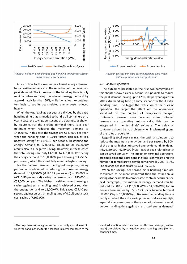
7/23/2019 Thesis Robert Heij Final Digital Version
http://slidepdf.com/reader/full/thesis-robert-heij-final-digital-version 92/94
92
Figure 8: Relation peak demand and handling time for restricting
maximum energy demand
A restriction to the maximum allowed energy demand
has a positive influence on the reduction of the terminals’
peak demand. The influence on the handling time is onlyminimal when reducing the allowed energy demand by
approximately less than 50%, while it enables the container
terminals to see its peak related energy costs reduced
hugely.
When the total savings per year are divided by the extra
handling time that is needed to handle all containers on a
yearly base, the savings per second are obtained, as shown
by Figure 9. For the 8-crane terminal there is a clear
optimum when reducing the maximum demand to
14,000kW. In this case the savings are €141,000 per year,
while the handling time is 0.01% faster. This results in a
negative saving 1 of €197.10 per second. Restricting the
energy demand to 17,000kW, 18,000kW or 19,000kW
results also in a negative saving. However, in these cases
the total savings are only €12,000 to €61,000. Restricting
the energy demand to 13,000kW gives a saving of €251.53
per second, which the absolutely seen the highest saving.
For the 6-crane terminal the highest (negative) saving
per second is obtained by reducing the maximum energy
demand to 12,000kW (-€180.27 per second) or 13,000kW
(-€115.86 per second), saving the terminal resp. €80,000 or
€53,000 per year. The highest positive value (meaning a
saving against extra handling time) is achieved by reducingthe energy demand to 11,000kW. This saves €79.40 per
second against an extra handling time of 0.01% and a total
cost saving of €107,000.
1 The negative cost saving per second is actually a positive result,
since the handling time for this scenario is lower compared to the
Figure 9: Savings per extra second handling time when
restricting maximum energy demand
5.3 Analysis of results
The outcomes presented in the first two paragraphs of
this chapter show a clear outcome: it is possible to reducethe peak demand, saving up to €250,000 per year against a
little extra handling time (in some scenarios without extra
handling time). The bigger the restriction of the rules of
operation, the larger the effect on the operations,
visualised by the number of temporarily delayed
containers. However, since more and more container
terminals are operating automatically, this can be
integrated in the terminals’ software. The delay of
containers should be no problem when implementing one
of the rules of operation.
Regarding total cost savings, the optimal solution is toreduce the maximum energy demand per second by 50%
of the original highest observed energy demand. By doing
this, €160,000 - €249,000 (40% - 48% of peak related costs)
can be saved annually. The impact on terminal operations
are small, since the extra handling time is only 0.1% and the
number of temporarily delayed containers is 2.2% - 3.7%.
The savings per second are €15.53 - €20.12.
When the savings per second extra handling time are
considered to be more important than the total annual
savings (for example to compensate container carriers, see
next paragraph), the maximum energy demand can be
reduced by 30% - 35% (13,000 kW/s - 14,000kW/s) for an
8-crane terminal or by 5% - 15% for a 6-crane terminal
(12,000 kW/s - 13,000kW/s). Because the handling time is
hardly affected, the extra savings per second are very high,
especially because some of these scenarios showed a small
quicker handling time against a restricted energy demand.
standard situation, which means that the cost savings (positive
result) are divided by a negative extra handling time (i.e. less
handling time).
0
1.000
2.000
3.000
4.000
0
5.000
10.000
15.000
20.000
25.000
I n f i n i t y
1 9 . 0 0 0
1 7 . 0 0 0
1 5 . 0 0 0
1 3 . 0 0 0
1 1 . 0 0 0
9 . 0 0 0
7 . 0 0 0
5 . 0 0 0
H a n d l i n g t i m
e ( h o u r s / y e a r )
P e a k
D e m a n d ( k W )
Energy demand limitation (kW/s)
PeakDemand HandlingTime (hours/year)
-€ 300
-€ 200
-€ 100
€ 0
€ 100
€ 200
€ 300
4.000 9.000 14.000 19.000
S a v i n g s p e r
s e c o n d e x t r a
h a n d l i n g t i m
e ( € / s e c . / y e a r )
Energy demand limitation (kW)
8 crane terminal 6 crane terminal
7/23/2019 Thesis Robert Heij Final Digital Version
http://slidepdf.com/reader/full/thesis-robert-heij-final-digital-version 93/94
93
When reducing the number of lifting quay cranes by 50%,
the peak related costs are reduced by approximately 40%
(saving up to €195,000 per year). The extra handling time
is only 0.37% - 0.44% (less than half a minute per hour
handling time) against a saving of €2.96 - €5.92 per second
extra handling time. By reducing the number ofsimultaneously lifting quay cranes by less than 50%, the
total savings are less, while the savings per second are not
increasing. By reducing the number of lifting quay cranes
by more than 50% the peak demand decreases even
further, but the handling time increases drastically. The
most optimal solution would therefore be to reduce the
number of simultaneously lifting quay cranes by 50%.
6 Implications of results
6.1
Extra handling time
Extra waiting time for containerships is something that iswatched critically by the container carriers. Despite the
critical attitude of cargo carriers towards waiting time in
ports, the adaption of containerships’ cruising speeds (also
known as slow steaming) is no issue. For container carriers,
their biggest costs are fuel. These costs might be reduced
by adapting the ship speed: a reduction to 80% saves 60%
fuel costs, while a reduction to 60% saves 90% of the fuel
costs (Wärtsilä, 2010). A market survey showed that 75%
of the surveyed liners and carriers apply slow steaming in
order to save bunker costs (Seatrade Global, 2014). Since
the fuel costs are that high, container carriers are operating
more efficient when sailing at lower speeds. In this regard
the extra travel time is compensated by fuel savings.
6.2
Costs containership
For handling 2,000 TEU of a containership (loading and
unloading) a terminal needs approximately 18 hours using
only three quay cranes. When extra handling time is
needed, the question is whether container carriers are
willing to accept this without any form of compensation. If
terminal operations take more time than agreed in
advance, carriers are compensated, known as demurrage
(Haugen Consulting, 2015). When a ship requires less time
than agreed on forehand, the terminal can request a bonus
for quicker handling, the so called despatch. This shows
that compensation is quite regular in the shipping business.
The question is therefore whether container terminals
are able to compensate container carriers to a certain
extent. To answer this question, first the costs for a
containership need to be determined. To determine the
annual costs for a containership, AECOM made a report for
the North Carolina Department of Transportation (2012).
They pointed out three cost aspects: the investment costs
for a containership, labour costs and fuel costs. The
purchase of a containership of 15,000 TEU (Emma Maersk
class) costs around 127 million euros (Maersk, 2006).
When dividing these costs over a lifespan of 30 years and
an annual discount rate of 6%, this is ±9 million euros per
year. Labour costs can be estimated at 1.2 million euros
(AECOM, 2012). Fuel costs can be neglected, since extrahandling time will not lead to extra fuel consumption.
Table 2: Cost containership per year, hour and second
Type of cost Costs
Investment costs € 9,000,000
Labour costs € 1,200,000
Total per year € 10,200,000
Total per hour € 1,164
Total per second € 0.32
Since a peak reduction of 50% saves a container terminal
at least €2.96-5.92 per second, this leaves room to
compensate the carriers for the extra handling time. This
could result in a win-win situation: container terminals
saving costs by reducing their peak demand and carriers
reducing their handling costs due to the compensation.
7 Conclusions
The objective of the research was to investigate the
opportunities for lowering the peak demand of ship-to-
shore crane operations at container terminals. When trying
to reduce the peak demand of container terminals by
implementing new rules of operation (i.e. reducing the
number of simultaneously lifting cranes or by limiting the
maximum energy demand), it is shown that the peak can
be reduced by 50% while impacting the handling time less
than half a minute per hour. A cost reduction of 50% saves
a container terminal with eight quay cranes and a
throughput of 1.6 million TEU up to €275,000 per year.
Despite the positive effect of cost savings, the reduction
of peak demand has consequences for the handling time.
In most scenarios (dependent on how much the number of
simultaneously lifting cranes and energy demand persecond is limited) the extra handling time would be less
than half a minute per hour. The question is whether
container carriers are willing to accept extra handling time.
Container terminals need to be prepared to negotiate with
container carriers about some sort of compensation. This
can be financially, but also regarding extra service (e.g. free
electricity power for ships while berthed) or sustainability
agreements. Despite the cost allocation, the research
showed that container terminals can reduce their peak
related energy costs by managing the energy consumption
in a smarter way.
7/23/2019 Thesis Robert Heij Final Digital Version
http://slidepdf.com/reader/full/thesis-robert-heij-final-digital-version 94/94
References
ABB. (2014, May 28). (R. Heij, Interviewer)
ABB. (2014). Data quay cranes.
AECOM. (2012). Vessel Size vs. Cost. AECOM.
Alessandri, A., Cervellera, C., Cuneo, M., Gaggero, M., & Soncin,
G. (2008). Modeling and Feedback Control forResource Allocation and Performance Analysis in
Container Terminals. IEEE Transactions on Intelligent
Transportation Systems, 9(4), 601-614.
Alessandri, A., Sacone, S., & Siri, S. (2007). Modelling and
Optimal Receding-horizon Control of Maritime
Container Terminals. Journal of Mathematical
Modelling and Algorithms, 6(1), 109-133.
APM Terminals. (2014, 05 20). Terminal information. Retrieved
from
http://www.apmterminals.com/asia/tanjungpelepas/t
erminalinfo.aspx?id=1888
Bortfeldt, A., & Gehring, H. (2001). A hybrid genetic algorithm
for the container loading problem. European Journal ofOperational Research, 131(1), 143-161.
Caballini, C., & Sacone, S. (2014). Modeling and Simulation of the
Rail Port Cycle. IEEE Systems Journal (99), 1-10.
Caballini, C., Pasquale, C., Sacone, S., & Siri, S. (2014). An Event-
Triggered Receding-Horizon Scheme for Planning Rail
Operations in Maritime Terminals. IEEE Transactions
on Intelligent Transportation Systems, 15(1), 365-375.
Cartenì, A., & De Luca, S. (2011). Tactical and strategic planning
for a container terminal: Modelling issues within a
discrete event simulation approach. Simulation
Modelling Practice and Theory (21), 123-145.
Clarksons. (2015, January 27). Clarksons, the heart of globalshipping. Retrieved from Containers:
http://www.clarksons.com/services/broking/container
s/
Dekker, R., Voogd, P., & Van Asperen, E. (2006). Advanced
methods for container stacking. OR Spectrum, 563-
586.
Eugen, R., Şerban, R., Augustin, R., & Ştefan, B. (2014).
Transshipment Modelling and Simulation of Container
Port Terminals. Advanced Materials Research, 837 ,
786-791.
Geerlings, H., & Van Duin, R. (2011). A new method for assessing
CO2-emissions from container terminals: a promising
approach applied in Rotterdam Journal of Cleaner
Imai, A., Sasaki, K., Nishimura, E., & Papadimitriou, S. (2006).
Multi-objective simultaneous stowage and load
planning for a container ship with container rehandle
in yard stacks. European Journal of Operational
Research(171), 373-389.
Lloyd's List. (2015, January 27). Lloyd's List Containerisation
International . Retrieved from MSC Oscar becomes theworld's largest boxship:
http://www.lloydslist.com/ll/news/article453843.ece
Maersk. (2006, September 08). Emma Maersk / Container vessel
specifications. Retrieved from http://www.emma-
maersk.com/specification/
MSC Terminal Valencia. (2009, December 3). Energy
consumption quay crane.
Port of Rotterdam. (2013, July). Focus on Vessels. Retrieved from
http://www.portofrotterdam.com/en/shipping/docum
ents/het-schip-centraal-eng-juli13.pdf
Seatrade Global. (2014, October 07). The economics of slow
steaming. Retrieved from http://www.seatrade-
global.com/news/americas/the-economics-of-slow-
steaming.html
Simio LLC. (2015). Simio Simulation Software.
Stahlbock, R., & Voß, S. (2008). Operations research at container
terminals: a literature update. OR Spectrum, 30(1), 1-
52.
Stedin. (2014). Electriciteit tarieven 2014 - aansluiting en
transport voor grootverbruikers. Rotterdam.
Steenken, D., Voß, S., & Stahlbock, R. (2004). Container terminal
operation and operations research. OR Spectrum,
26:3-49.
UNCTAD. (2013). Review of maritime transport. New York and
Geneva: United Nations Publication.
Van Asperen, E., Borgman, B., & Dekker, R. (2010). Evaluating
container stacking rules using simulation. Proceedings
of the 2010 Winter Simulation Conference.
Van der Voet, M. (2008). CO2‐emissie door
containeroverslagprocessen in de Rotterdamse haven.
Delft.
Van Duin, R., & Geerlings, H. (2011). Estimating CO2-footprints
of container terminal port-operations. International
Journal of Sustainable Development and Planning, 459-
473.
Wärtsilä. (2010, February). Slow steaming - a viable long-term
option? Retrieved from