thesis pdf, 2mb
TRANSCRIPT
Dissertation
submitted to the
Combined Faculties of the Natural Sciences and Mathematics
of the Ruperto-Carola-University of Heidelberg. Germany
for the degree of
Doctor of Natural Sciences
Put forward by
Eva Lefa
born in Athens, Greece
Oral examination: 21th November 2012

Non-thermal Radiation
processes in relativistic
outflows from AGN
Referees: Prof. Dr. Felix A. Aharonian
Prof. Dr. Werner Hofmann

Abstract
Non-thermal, leptonic radiation processes have been extensively studied for the in-terpretation of the observed radiation from jets of Active Galactic Nuclei (AGN).This work addresses the synchrotron and Inverse Compton scattering (ICS) mecha-nisms, and investigates the potential of a self-consistent, time-dependent approachto currently unsolved problems. Furthermore, it examines how deviations from stan-dard, one-zone models can modify the radiated spectrum. A detailed analysis of theshape of the ICS spectrum is also performed.In the rst part a possible interpretation of the hard γ-ray blazar spectra in theframework of leptonic models is investigated. It is demonstrated that hard γ-rayspectra can be generated and maintained in the presence of energy losses, under thebasic assumption of a narrow electron energy distribution (EED). Broader spectracan also be modeled if multiple zones contribute to the emission. In such a scheme,hard aring events, like the one in Mkn 501 in 2009, can be successfully interpretedwithin a "leading blob" scenario, when one or few zones of emission become domi-nant.In the second part the shape of the Compton spectrum close to the maximum cut-o is investigated. Analytical approximations for the spectral shape in the cutoregion are derived for various soft photon elds, providing a direct link between theparent EED and the upscattered spectrum. Additionally, a generalization of thebeaming pattern for various processes is derived, which accounts for non-stationary,anisotropic and non-homogeneous EEDs. It is shown that anisotropic EEDs maylead to radiated spectra substantially dierent from the isotropic case. Finally, aself-consistent, non-homogeneous model describing the synchrotron emission fromstratied jets is developed. It is found that transverse jet stratication leads tocharacteristic features in the emitted spectrum dierent to expectations in homoge-neous models.
Zusammenfassung
Bezüglich der Herkunft der beobachteten Strahlung von Jets in Aktiven Galaktis-chen Kernen (AGN) wurden nicht-thermische, leptonische Strahlungsprozesse in-tensiv untersucht. In der vorliegenden Arbeit wird die Strahlungserzeugung durchSynchrotron-Emission und inverse Compton-Streuung (ICS) diskutiert und das Po-tential eines selbstkonsistenten, zeitabhängigen Models zur Erklärung aktuell nochungelöster Probleme analysiert. Des Weiteren werden die Auswirkungen von Abwe-ichungen von Standardmodellen auf das emittierte Spektrum untersucht. Die Formder ICS-Spektren wird im Detail diskutiert.Im ersten Teil dieser Arbeit wird eine mögliche Erklärung der harten Gammastrahlen-Spektren von Blasaren im Rahmen eines leptonischen Models untersucht. Dabeiwird gezeigt, dass sich harte Gammastrahlenspektren bei Annahme einer schmalenElektronen-Energieverteilung (EED) auch angesichts von Energieverlusten erzeugenund erhalten lassen. Breitere Emissionsspektren können durch Überlagerung vonBeiträgen verschiedener Zonen generiert werden. In diesem Zusammenhang könnenharte Emissionsereignisse, wie z.B. das in 2009 für Mkn 501 beobachtete, durch ein"leading-blob" Szenario, bei dem eine oder mehrere Zonen dominieren, erfolgreicherklärt werden.Im zweiten Teil wird das Compton-Spektrum nahe der maximalen Energie der EEDuntersucht. Die in dieser Arbeit hergeleiteten, analytischen Näherungen für die Formdes Compton-Spektrums erlauben eine direkte Verbindung des gestreuten Emission-sspektrums mit der erzeugenden EED für verschiedene (soft photon) Felder. Auÿer-dem wird eine Verallgemeinerung des relativistischen "beaming patterns" für denFall nicht-stationärer, anisotroper und inhomogener EEDs hergeleitet. AnisotropeEEDs können dabei zu Spektren führen, die sich erheblich vom isotropen Fall unter-scheiden. Zuletzt wird, motiviert durch neuere Simulations- und Beobachtungsergeb-nisse, ein selbstkonsistentes (Synchrotron) Emissionsmodel entwickelt, bei dem derzugrundeliegende Jet eine transversale Abhängigkeit (parallele Scherströmung) auf-weist. Dabei zeigt sich, dass eine transversale Abhängigkeit zu charakteristischenEigenschaften des emittierten Spektrums führt, die sich signikant von den Er-wartungen homogener Modelle unterscheiden und damit Einblick in die Jetstrukturgeben.
Contents
1 Introduction 1
1.1 Basic properties and the physics of AGN . . . . . . . . . . . . . . . . 1
1.1.1 The general picture of AGN . . . . . . . . . . . . . . . . . . . 1
1.1.2 Unication schemes and classication of AGN . . . . . . . . . 4
1.1.3 Blazars: properties and observed spectrum . . . . . . . . . . . 5
1.2 Radiation processes in leptonic models . . . . . . . . . . . . . . . . . 8
1.2.1 Synchrotron radiation . . . . . . . . . . . . . . . . . . . . . . 8
1.2.2 Inverse Compton Scattering . . . . . . . . . . . . . . . . . . . 10
1.3 A self-consistent approach: kinetic equation of electrons . . . . . . . . 12
1.4 Interaction with the EBL . . . . . . . . . . . . . . . . . . . . . . . . . 16
1.5 Aim of this thesis . . . . . . . . . . . . . . . . . . . . . . . . . . . . . 18
2 Formation of hard VHE γ-ray Blazar spectra 21
2.1 The puzzle of hard γ-ray Blazar spectra . . . . . . . . . . . . . . . . 21
2.2 Suggested solutions . . . . . . . . . . . . . . . . . . . . . . . . . . . . 23
2.3 Stationary SSC with an energetic electron distribution . . . . . . . . 25
2.3.1 Power-law electron distribution with high value of low-energy
cuto . . . . . . . . . . . . . . . . . . . . . . . . . . . . . . . 26
2.3.2 Relativistic Maxwellian electron distribution . . . . . . . . . . 28
2.4 Time dependent case - expansion of the source . . . . . . . . . . . . . 32
2.5 The external Compton scenario . . . . . . . . . . . . . . . . . . . . . 36
2.6 Summary and application to 1ES 0229+200 . . . . . . . . . . . . . . 38
3 "Leading blob" model in a stochastic acceleration scenario 43
3.1 The 2009 hard are of Mkn 501 . . . . . . . . . . . . . . . . . . . . . 43
3.2 A multi-zone scenario . . . . . . . . . . . . . . . . . . . . . . . . . . . 46
3.3 The origin of hard γ-ray spectrum ares . . . . . . . . . . . . . . . . 50
3.4 The case of the Quasar 3C279 . . . . . . . . . . . . . . . . . . . . . . 53
i
3.5 Conclusion . . . . . . . . . . . . . . . . . . . . . . . . . . . . . . . . . 53
4 On the spectral shape of radiation due to Inverse Compton Scat-
tering close to the maximum cut-o 57
4.1 On ICS and the importance of the maximum cuto . . . . . . . . . . 57
4.2 Compton spectrum for monochromatic photons . . . . . . . . . . . . 59
4.2.1 Thomson Regime . . . . . . . . . . . . . . . . . . . . . . . . . 60
4.2.2 Klein-Nishina Regime . . . . . . . . . . . . . . . . . . . . . . . 62
4.3 Compton spectrum for a broad photon distribution . . . . . . . . . . 65
4.3.1 Planckian photon eld . . . . . . . . . . . . . . . . . . . . . . 65
4.3.2 Synchrotron photon eld . . . . . . . . . . . . . . . . . . . . . 67
4.3.3 Synchrotron spectrum . . . . . . . . . . . . . . . . . . . . . . 67
4.3.4 SSC spectrum . . . . . . . . . . . . . . . . . . . . . . . . . . . 69
4.4 Cooled electron distribution . . . . . . . . . . . . . . . . . . . . . . . 73
4.5 Comparison of the results . . . . . . . . . . . . . . . . . . . . . . . . 74
4.6 The cuto energy of the Compton spectrum . . . . . . . . . . . . . . 76
4.7 Summary . . . . . . . . . . . . . . . . . . . . . . . . . . . . . . . . . 77
5 On radiation boosting due to relativistic motion
and eects of anisotropy 79
5.1 Introduction . . . . . . . . . . . . . . . . . . . . . . . . . . . . . . . . 79
5.2 Photon transfer . . . . . . . . . . . . . . . . . . . . . . . . . . . . . . 80
5.3 Non-isotropy . . . . . . . . . . . . . . . . . . . . . . . . . . . . . . . . 83
5.4 Conclusions . . . . . . . . . . . . . . . . . . . . . . . . . . . . . . . . 87
6 Leptonic radiation from stratied jets 89
6.1 Evidence for non-homogeneous outows . . . . . . . . . . . . . . . . . 89
6.2 Relativistic jet with stratication at the transverse direction . . . . . 92
6.3 Properties of the layers . . . . . . . . . . . . . . . . . . . . . . . . . . 97
6.3.1 Electron distribution integrated over the longitudinal direction 97
6.3.2 Intrinsic synchrotron emission from each layer . . . . . . . . . 99
6.4 Parametrization of the physical parameters . . . . . . . . . . . . . . . 101
6.5 Total observed synchrotron spectrum . . . . . . . . . . . . . . . . . . 104
6.5.1 Total, volume integrated, electron distribution . . . . . . . . . 104
6.6 Eects of the maximum energy of the injected electron distribution . 111
6.7 Summary and future work on stratied outows . . . . . . . . . . . . 112
7 Conclusions 115
ii
Chapter 1
Introduction
1.1 Basic properties and the physics of AGN
Relativistic jets are common in astrophysical environment. Active Galactic Nu-clei (AGN), Gamma Ray Bursts (GRBs) and microquasars have been proven toexhibit highly collimated outows in which particles are accelerated to relativisticenergies and radiate. Among these sources, AGN are of particular interest. Theyprovide an excellent environment for investigating several aspects of modern as-trophysics; accretion, formation and collimation of jets, magnetohydrodynamics,particle acceleration theories and radiation mechanisms, all come into play. Addi-tionally, AGN are directly related to the question of galaxy evolution. Since thediscovery of Quasars (Schmidt 1963), these object have been the most prominentemitters among the most luminous and distant objects in the universe and haverightfully attracted particular astrophysical interest.
1.1.1 The general picture of AGN
In general, AGN are galaxies with energetic phenomena in their nuclei (centralregion) which can not be directly attributed to stellar processes. AGN produce veryhigh luminosities, of the order of 1046−1048erg/sec, (four orders of magnitude higherthan the luminosity of a typical galaxy) in a centered, compact volume (within par-sec scales). Their continuum spectra is attributed to radiation from non-thermalprocesses and can emerge over a wide range of the electromagnetic spectrum, fromvery low radio frequencies up to TeV γ-rays. Strong variability (increase in lumi-nosity by a factor of ∼ 2 or more) is present on various timescales, from years downto less than a day, even on minute-timescales (Aharonian et al. 2007). The SpectralEnergy Distribution (SED) of these objects often exhibit emission (and occasion-ally absorption) lines indicating excitation by the continuum emission. Roughlyspeaking, a galaxy can be dened as AGN if it exhibits some of the aforementionedcharacteristic features (not necessarily all of them at the same time) and around1− 3% of the whole galaxy population can be accounted as AGN.
Nowadays, the generally accepted picture for the fueling and the observed prop-erties of AGN is based on the existence of a rotating, supermassive black hole at the
1
1.1. Basic properties and the physics of AGN
center of the galaxy. The supermassive black hole (SMBH) is surrounded by a thindisk which accretes gas with angular momentum onto the SMBH (Salpeter, 1964;Zeldovich & Novikov, 1964). The release of the gravitational energy of the infallingmatter is ultimately responsible for the large radiative output of those objects. Ac-cretion onto a compact object is thus regarded to be the principal source of energyfor AGN.
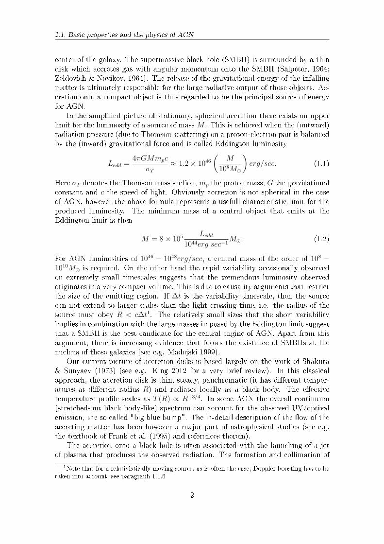
In the simplied picture of stationary, spherical accretion there exists an upperlimit for the luminosity of a source of mass M . This is achieved when the (outward)radiation pressure (due to Thomson scattering) on a proton-electron pair is balancedby the (inward) gravitational force and is called Eddington luminosity
Ledd =4πGMmpc
σT≈ 1.2× 1046
(M
108M⊙
)erg/sec. (1.1)
Here σT denotes the Thomson cross section, mp the proton mass, G the gravitationalconstant and c the speed of light. Obviously accretion is not spherical in the caseof AGN, however the above formula represents a usefull characteristic limit for theproduced luminosity. The minimum mass of a central object that emits at theEddington limit is then
M = 8× 10⁵Ledd
1044erg sec−1M⊙. (1.2)
For AGN luminosities of 1046 − 1048erg/sec, a central mass of the order of 108 −1010M⊙ is required. On the other hand the rapid variability occasionally observedon extremely small timescales suggests that the tremendous luminosity observedoriginates in a very compact volume. This is due to causality arguments that restrictthe size of the emitting region. If ∆t is the variability timescale, then the sourcecan not extend to larger scales than the light crossing time, i.e. the radius of thesource must obey R < c∆t1. The relatively small sizes that the short variabilityimplies in combination with the large masses imposed by the Eddington limit suggestthat a SMBH is the best candidate for the central engine of AGN. Apart from thisargument, there is increasing evidence that favors the existence of SMBHs at thenucleus of these galaxies (see e.g. Madejski 1999).
Our current picture of accretion disks is based largely on the work of Shakura& Sunyaev (1973) (see e.g. King 2012 for a very brief review). In this classicalapproach, the accretion disk is thin, steady, panchromatic (it has dierent temper-atures at dierent radius R) and radiates locally as a black body. The eectivetemperature prole scales as T (R) ∝ R−3/4. In some AGN the overall continuum(stretched-out black body-like) spectrum can account for the observed UV/optivalemission, the so called "big blue bump". The in-detail description of the ow of theaccreting matter has been however a major part of astrophysical studies (see e.g.the textbook of Frank et al. (1995) and references therein).
The accretion onto a black hole is often associated with the launching of a jetof plasma that produces the observed radiation. The formation and collimation of
1Note that for a relativistically moving source, as is often the case, Doppler boosting has to betaken into account, see paragraph 1.1.6
2
1.1. Basic properties and the physics of AGN
jets has been intensively studied in the hydrodynamical (HD) and magnetohydrody-namical (MHD) formulation by applying both analytical and numerical techniques.One can distinguish three main types of models (see e.g. Celotti & Blandford, 2001;Sauty et al., 2002 for reviews).
(a) Hydrodynamical acceleration: An adiabatic ow that propagates in theexternal medium of decreasing pressure can get accelerated and collimated as in ade Laval nozzle, as proposed in the so called "twin-exhaust" model of Blandford &Rees (1974). The "weak point" of such a model is that the required gas pressureneeded from the external medium implies a large X-ray ux which is not observed.
(b) Radiative acceleration: Acceleration by radiation pressure could in prin-ciple explain the relativistic jets observed in AGN. This mechanisms is based onradiation beams that are produced and collimated in funnels (vortices) along therotational axis of the accretion disk (see e.g. Lynden-Bell, 1978; Piran, 1982). How-ever, intense radiation elds are required and even if they exist Compton drag limitsseverely the velocity of the ow.
(c)Magnetohydrodynamical acceleration: Perhaps the most promising mech-anism for the production of jets involve magnetic elds. Extraction of energy mayoccur from the accretion disk as an MHD wind is launched due to centrifugal forceif the angle between the poloidal component of the magnetic eld and and thedisk surface is 60o. Alternatively, the relativistic jet can be powered by the rotatingblack hole itself (Runi & Wilson, 1975; Lovelace, 1976; Blandford & Znajek, 1977).
Independent of the formation mechanism, relativistic jets do occur in AGN andcan range from sub-parsec scales out to Mpc scales. Perhaps, the most direct ev-idence for high speeds is superluminal motion. VLBI (Very Long Baseline Inter-ferometry) observations of some sources have detected radio components that showtransverse (apparent) velocities that exceed the speed of light even up to ∼ 40c.This discrepancy with special relatively can be solved only if the outow moves atrelativistic speeds close to the line of sight (Rees 1966). The transverse apparentvelocity βapp with respect to the "real" velocity β is
βapp =β sin θ
1− β cos θ. (1.3)
Thus for relativistically moving sources, β > 1/√2 ∼ 0.7, there exist some values of
the orientation angle θ at which superluminal motion is observed. The maximumapparent velocity occurs at sin θ = 1/Γ, where Γ = (1−β2)−1/2 is the Lorentz factor,and takes the value βmaxapp =
√(Γ2 − 1). This means that if an apparent velocity of
e.g. βapp = 5 is detected, then the source has to move relativistically as it can nothave Lorentz factor less than Γmin =
√β2app + 1, providing strong evidence for the
existence of relativistic jets.The observed, non-thermal, continuum spectrum is commonly attributed to the
radiation of particles that accelerate to highly relativistic energies in the jets. Apart
3
1.1. Basic properties and the physics of AGN
from the continuum, broad emission lines are often detected. These are consideredto originate from rapidly moving clouds of gas above the accretion disk that mayextend up to 103Rg, where Rg the Schwarzschild radius. The area where these cloudsare located is commonly abbreviated as Broad Line Region (BLR). Above the BLRthere are slower-moving clouds that can extend as far as 1020cm and are responsiblefor the narrow lines that may exist in the SED of some AGN. The main picture ofAGN is completed with the existence of a dusty torus around the central object thatobscures the radiation from the inner parts if the line of sight passes through thistorus.
In summary, the commonly accepted picture for AGN (on a very rst approach)has been formulated as following:
• A supermassive, rotating black hole in the center of the galaxy of mass 108 −1010M⊙;
• A thin disk accreting onto the SMBH, from about 2 to beyond 100 gravita-tional radii that emits mainly at UV and soft X-rays (though it is sometimesresponsible for the hard X-rays as well);
• The BLR which extends up to ∼ 103Rg and scatters away the radiation fromthe inner parts;
• The NLR which extends from 104-106Rg;• A dusty torus (with an inner radius of ∼ 103Rg) which obscures the centralparts of the AGN emission.
1.1.2 Unication schemes and classication of AGN
The numerous sources identied as AGN exhibit dierent observational charac-teristics and their classication according to phenomenological properties is rathercomplex. In a very simplied picture, AGN can be divided to sub-classes by twomain parameters; the radio-loudness and the width of the emission lines (see e.g.Padovani 1999). Approximately 10% of the AGN population is radio-loud, i.e. theirradio luminosity exceed the optical luminosity by a factor of ten, Lrad/Lopt ∼ 10.According to the width of their emission lines, AGN can be further divided intotype I (broad line emission galaxies; they exhibit lines that correspond to velocitiesof the clouds of the order of 2, 000− 10, 000km/sec) and type II (narrow line emis-sion galaxies with corresponding velocities of ∼ 500km/sec). For example, SeyfertI and Seyfert II/radio-quiet Quasars (QSOs) are radio-quiet AGN of type II and Irespectively. Radio-loud type II AGN are called narrow-line radio galaxies (NLRG).Radio-loud type I AGN are referred as broad-line radio galaxies (BLRGs). Ac-cording to their radio morphology radiogalaxies of both types are also classied asFanaro-Riley (FR) I and II . Some objects have very weak emission lines, like theso called BL Lacs which are radio-loud.
Although AGN appear dierent, unication schemes support the idea that theyare not truly dierent objects. On the contrary, they share the same intrinsic prop-erties but they are viewed under dierent angles (see the reviews of Antonucci,1993; Urry & Padovani, 1995). The observed radiation might e.g. be strongly en-hanced due to Doppler boosting if the jet is pointing towards the observer or it can
4
1.1. Basic properties and the physics of AGN
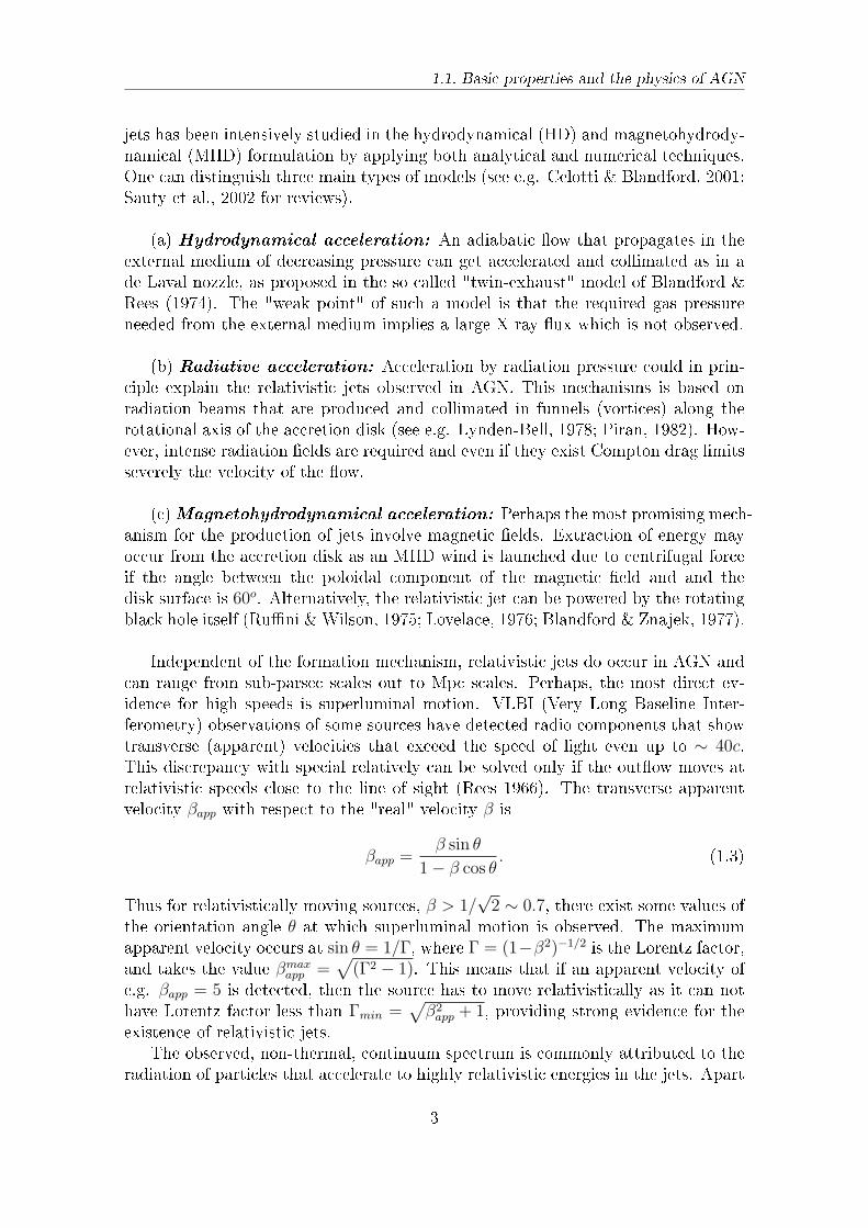
be obscured by the torus if the viewing angle is large (see g. 1.1) so that onlythe NLR can be seen. For example, Seyfert I galaxies have been "unied" withSeyfert II galaxies with the former be seen edge-on (large viewing angles) and thelatter face-on (small viewing angles). In a similar way low-luminosity FR I sourcesand high luminosity FR II radio galaxies correspond to BL Lacs and radio Quasarsrespectively.
Jet
Obscuring Torus
Black Hole
Narrow Line Region
Broad Line Region
Accretion Disk
Figure 1.1: Sketch illustrating the unied picture of AGN (not to scale). Figurefrom Urry & Padovani (1995)
1.1.3 Blazars: properties and observed spectrum
A sub-class of AGN of particular interest are the so called Blazars. Blazarsare radio sources that apparently exhibit the most extreme characteristics; rapidvariability (at all wavelengths and on all timescales), high polarization (both inoptical and radio frequencies) and in some cases a lack of any strong emission lines.Blazars are characterized by broadband (from radio to VHE γ-rays), non-thermalemission produced in relativistic jets pointing close to the line of sight to the observerand thus their observed radiation is strongly boosted. This group of AGN includesthe Optically Violent Variable Quasars (OVVs) which are characterized by rapidvariability, highly polarized Quasars (HPQs) that exhibit high percentage of linearpolarization, the aforementioned BL Lacs and the Flat Spectrum Radio Quasars(FSRQs) that tend to have at radio spectra, i.e. Fν ∝ ν−α with α > −0.5. Thename "Blazars" originates from the astronomer Ed Spiegel, likely as an attempt tocombine the names of BL Lacs and Quasars.
5
1.1. Basic properties and the physics of AGN
Blazars rightfully hold a special place among all AGN. Their broad band emissioncovers almost 20 orders of magnitude along the electromagnetic spectrum, and thusthey are ideal sources for multiwavelength studies. They are very often strong γ-rayemitters (up to TeV energies), implying that very energetic phenomena take place.The relativistic beaming of the radiation amplies the brightness of these sourcesso that they are prominent for detection even at low luminosities, or equivalently atlarge distances. Due to this strong enhancement, the spectrum of Blazars is highlydominated by the jet emission. The "noise" that originates from other parts ofthe galaxy (accretion disk, BLR, torus etc..) is likely suppressed. For this reasonBlazars serve to dene the properties of the jet and to study the associated physicsthat takes place in relativistic outows.
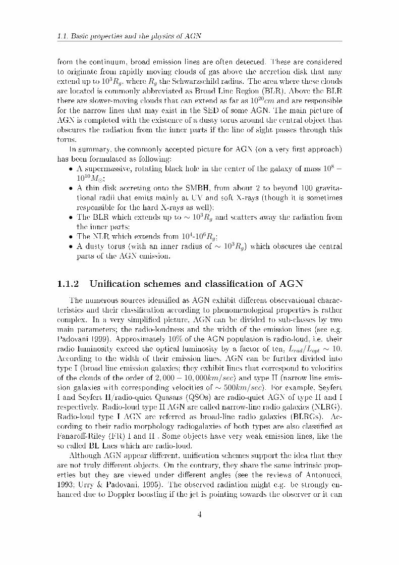
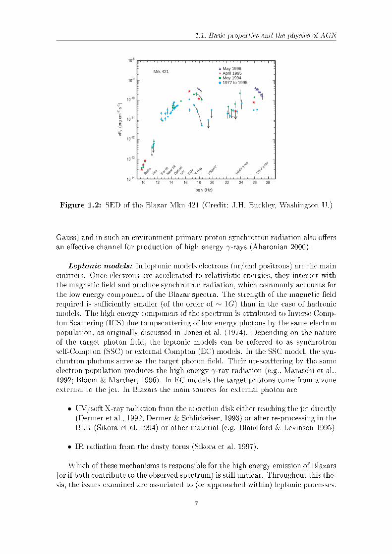
The continuum Spectral Energy Distribution (SED) of Blazars extends fromthe low frequency radio band up to TeV γ-rays. It is dominated by non-thermalemission and often shows two distinct components. A low-energy component fromradio up to UV and X-rays and a high energy component from X-rays to γ-rays(see e.g. the SED of the Blazar Mkn 421 in g. 1.2). Variability characterizes allemission wavelengths and particularly at high energies very short timescales (downto minutes) have been reported (e.g. Aharonian et al., 2007; Albert et al., 2007). Dueto Lorentz transformations the observed variability timescales ∆tobs are connectedto the intrinsic (comoving) timescale ∆tint as
∆tobs = ∆tint(1 + z)/D (1.4)
where D is the Doppler factor and z the cosmological redshift. Causality argumentsthen limit the source size to
R . c∆tobsD/(1 + z), (1.5)
implying that the emission originates in a very compact region.Theoretical radiation models that attempt to interpret the observed Blazar spec-
tra can be divided into two main categories, hadronic and leptonic models (see e.g.a recent review from Boettcher 2012). Hadronic models propose that the main car-riers of dissipated energy in the jet are energetic protons, whereas in leptonic modelsthe energy available for radiation is in electrons or e± pairs.
Hadronic models: Energetic photons can emit γ-rays via pp interaction withsurrounding gas or via pγ interaction with a photon eld. π0-decay γ-rays can beproduced in pp interactions, but very high densities of thermal plasma are requiredto explain the observed high luminosities (see e.g. Morrison et al. 1984). Alterna-tively, if protons are aectively accelerated to the threshold for pγ pion production,then synchrotron supported cascades will initiate (Mannheim, 1993; Mannheim &Biermann, 1992), i.e. protons will interact with the synchrotron photons producedby electrons that are co-accelerated with the protons (external photon elds mayalso be a possibility, e.g. thermal photons from the disk, Protheroe 1997). Electro-magnetic cascades can be initiated by π0-decay, electrons from the π± → µ± → e±
decay, p-synchrotron photons and µ, π and K synchrotron photons. Proton accel-eration to such high energies requires large magnetic elds (of the order of tens of
6
1.1. Basic properties and the physics of AGN
10 12 14 16 18 20 22 24 26 28
log ν (Hz)
10-14
10-13
10-12
10-11
10-10
10-9
10-8
νF
(erg
cm
-2 s
-1)
Radio
mm
Far I
RNea
r IR
Optica
l
EUVX-R
ay
100k
eV
1GeV
γ-ra
y
1TeV
γ-ra
y
Mrk 421May 1996 April 1995 May 1994 1977 to 1995
ν
UV
Figure 1.2: SED of the Blazar Mkn 421 (Credit: J.H. Buckley, Washington U.)
Gauss) and in such an environment primary proton synchrotron radiation also oersan eective channel for production of high energy γ-rays (Aharonian 2000).
Leptonic models: In leptonic models electrons (or/and positrons) are the mainemitters. Once electrons are accelerated to relativistic energies, they interact withthe magnetic eld and produce synchrotron radiation, which commonly accounts forthe low energy component of the Blazar spectra. The strength of the magnetic eldrequired is suciently smaller (of the order of ∼ 1G) than in the case of hadronicmodels. The high energy component of the spectrum is attributed to Inverse Comp-ton Scattering (ICS) due to upscattering of low energy photons by the same electronpopulation, as originally discussed in Jones et al. (1974). Depending on the natureof the target photon eld, the leptonic models can be referred to as synchrotronself-Compton (SSC) or external Compton (EC) models. In the SSC model, the syn-chrotron photons serve as the target photon eld. Their up-scattering by the sameelectron population produces the high energy γ-ray radiation (e.g., Maraschi et al.,1992; Bloom & Marcher, 1996). In EC models the target photons come from a zoneexternal to the jet. In Blazars the main sources for external photon are
• UV/soft X-ray radiation from the accretion disk either reaching the jet directly(Dermer et al., 1992; Dermer & Schlickeiser, 1993) or after re-processing in theBLR (Sikora et al. 1994) or other material (e.g. Blandford & Levinson 1995)
• IR radiation from the dusty torus (Sikora et al. 1997).
Which of these mechanisms is responsible for the high energy emission of Blazars(or if both contribute to the observed spectrum) is still unclear. Throughout this the-sis, the issues examined are associated to (or approached within) leptonic processes.
7
1.2. Radiation processes in leptonic models
The main radiation mechanisms involved (synchrotron and ICS) are presented inthe next paragraph, and they are embedded in a self-consistent approach.
Perhaps the two most triggering features in Blazar physics that have attractedspecial attention are the variability detected at very short timescales and the origin ofvery hard, intrinsic γ-ray source spectra after correcting for the absorption due to theExtragalactic Background Light (EBL). Although the observed TeV spectra of thesesources are steep, their de-absorbed (EBL-corrected) spectra appear intrinsicallyhard (see section 1.4). In chapter 2 we deal with this problem, proving a self-consistent solution with leptonic models. Furthermore, in chapter 3 we examine thepossibility to account for hard spectra in a aring state that normally (in a lowstate) are softer.
1.2 Radiation processes in leptonic models
Radiation mechanisms hold an outstanding place in astrophysics, as they areour "eyes" to the astrophysical objects of the universe. Emission processes are therst step to explore the physical mechanisms that take place in a variety of sourcesand thus, a deep understanding and in-detail investigation is unavoidably neces-sary. In this thesis we focus on leptonic models and the main processes involved aresynchrotron radiation and ICS. These radiation mechanisms have been intensivelystudied and remain two of the basic emission mechanisms that account for observa-tions not only in Blazars and AGN in general, but also for a series of astrophysicalobjects, e.g. pulsars, microquasars, GRBs etc.
1.2.1 Synchrotron radiation
Classically, a charged particle which moves on a curved path or is acceleratedon a straight-line path will emit electromagnetic radiation. When the reason ofacceleration is a magnetic eld then the radiation is called synchrotron radiation (forrelativistic particle velocities). Synchrotron radiation was rst suggested by Alfvén& Herlofson (1950) to be the radiation mechanism responsible for the newly (backthen) discovered cosmic radio sources (such as supernova remnants and AGN). Sincethen it has been investigated extensively in several textbooks and in the contextof astrophysical applications (Jackson, 1975; Rybicki & Lightmann, 1979; Longair,2010).
In the presence of a (uniform) magnetic eld of strength B, a charged particlewill gyrate around the eld lines at helical trajectory. From the equations of motionwe can nd the frequency of rotation
ωB =qB
γmc. (1.6)
If we denote by α the pitch angle (the angle between the eld and the particlevelocity) then in the limit of relativistic velocities (u ≈ c) the total emitted poweris
−(dE
dt
)= 2σT cUBγ
2 sinα2, (1.7)
8
1.2. Radiation processes in leptonic models
where UB = B2/8π is the magnetic eld energy density and σT the Thomson crosssection. For an isotropic particle distribution, averaging over pitch angles leads tothe formula
−(dE
dt
)=
4
3σT cUBγ
2. (1.8)
The derivation of the synchrotron spectrum from the Lienard-Wiechert poten-tials is well established and can be found in the aforementioned textbooks. Somemain points are the following: Due to light abberation eects the radiation of a rel-ativistic particle (in the frame of the observer) is beamed within a cone of openingangle ∼ 1/γ. A distant observer will thus receive pulses of radiation and the spec-trum is the Fourier transform of these pulses once time delay eects are taken intoaccount. The duration of the pulse is ∆t ≈ (γ3ωB sinα)−1 and thus the spectrumextends roughly up to the critical frequency
ωc =3γ2qB sinα
2mc. (1.9)
The full expression for the emitted spectrum for monoenergetic electrons of energyEe is
dNγ
dϵγ=
√3q3B sinα
mc2hϵγF
(ϵγEc
), (1.10)
where
Ec = ~ωc =3qBh sinα
4πmc
E2e
(mc2)2, (1.11)
and the function F (x) is given in terms of the modied Bessel function K5/3(ξ)
F (x) ≡ x
∫ ∞
x
K5/3(ξ)dξ. (1.12)
The synchrotron spectrum peaks at ∼ 0.29Ec. The function F (x) for small andlarge values of x has the asymptotic form
F (x) ∼
4π√
3Γ(1/3)
(x2
)1/3, x ≪ 1
(π2
)1/2x1/2e−x, x ≫ 1
(1.13)
where Γ(x) the Gamma function. Already from the above formula we expect thesynchrotron spectrum at low energies to exhibit a dependance on energy as ϵ
1/3γ
and at high energies to have a (simple) exponential cuto. For randomly orientedmagnetic elds, one needs to integrate over the pitch angles, i.e. dene the function
G(x) =
∫sinαF (x)dΩ/4π =
1
2
∫ π
0
F (x) sin2 αdα = x
∫ ∞
x
K5/3(ξ)
√1− x2
ξ2dξ.
(1.14)The function G(x) can be expressed analytically in terms of modied Bessel func-tions (or alternatively in terms of Whittaker's functions, Crusius & Schlickeiser
9
1.2. Radiation processes in leptonic models
1986), but there are also approximation formulas in terms of simple polynomials(see e.g. Melrose, 1980; Zirakashvili & Aharonian, 2007). Throughout this thesis,we have used the approximations derived in Aharonian et al. (2010), which providean accuracy better than 0.2% over the entire range of variable x
G(x) =1.808x1/3
√1 + 3.4x2/3
1 + 2.21x2/3 + 0.347x4/3
1 + 1.353x2/3 + 0.217x4/3e−x. (1.15)
These functions correspond to relativistic and monoenergetic electrons interactingwith tangled magnetic elds. There are, however, some interesting deviations fromthese standard formulas. For example, an exception may occur if the magnetic eldin the source would be fully turbulent with zero mean component. In such a case,the low-frequency part of the synchrotron spectrum could be harder than Fϵγ ∝ ϵ
1/3γ
(Medvedev, 2006; Derishev et al., 2007; Reville & Kirk, 2010). Furthermore, if thepitch angles of the particles are very small (less than 1/γ) then the emission diersqualitatively from the usual synchrotron emission in the sense that it peaks at lowerenergies and it falls o linearly at small frequencies, ϵγ (Epstein, 1973; Epstein &Petrosian, 1973).
In astrophysical problems we often encounter power-law electron distributions(see also paragraph 1.2.2) of the form
dNe/dEe ∝ E−pe Θ(Ee − Emin)Θ (Emax − Ee) , (1.16)
between a minimum and maximum energy, Emin and Emax, respectively. Here Θ(x−x0) is the step function. The synchrotron radiation spectrum is then a power-law,the index of which is related to the electron distribution index,
ϵγdNγ/dϵγ ∝ ϵ− p−1
2γ (1.17)
and it spreads roughly from Eminγ ∝ BE2
min to Emaxγ ∝ BE2
max, where B is themagnetic eld. Below the low energy cuto Emin
γ the functional dependance ofthe spectrum on the radiated photon energy is the same as the synchrotron kernelfunction, i.e. ϵγdNγ/dϵγ ∝ ϵ
1/3γ . This feature is discussed in chapter 2 where we
investigate the assumption of a large value for the minimum cuto of the electrondistribution for the interpretation of the hard spectrum sources, i.e. we examinehow both synchrotron and ICS appear in this case. In chapter 4 we also refer to theshape of the synchrotron spectrum close to the maximum cuto not only in the caseof a sharp, abrupt cuto for the electron distribution, but under the more generalassumption of an exponential cuto shape.
1.2.2 Inverse Compton Scattering
The interaction of relativistic electrons with low energy radiation through InverseCompton Scattering (ICS) provides one of the principal γ-ray production processesin astrophysics. In a variety of astrophysical environments, from very compact ob-jects like pulsars and Active Galactic Nuclei (AGN) to extended sources like super-nova remnants and clusters of galaxies, low energy photons are eectively boostedto high energies through this mechanism.
10
1.2. Radiation processes in leptonic models
In the ICS process low energy photons of energy ϵγ are up-scattered by relativisticelectrons to higher energies Eγ. The basic features of the ICS have been analyzedby Jones (1968), Blumenthal & Gould (1970). An extensive analysis can be found inthe aforementioned textbooks (Jackson, 1975; Rybicki & Lightmann, 1979; Longair,2010). The total cross section of ICS is derived in quantum electrodynamics. In thecase of isotropic photons and electrons it can be shown that the spectrum of highenergy photons generated per unit time due to ICS from monoenergetic electrons is(see e.g. Blumenthal & Gould (1970))
dNγ/dEγ =
∫ ∞
0
W (Ee, ϵγ, Eγ)nph(ϵγ)dϵγ, (1.18)
where
Eemin =1
2Eγ
(1 +
√1 +
m2c4
ϵγEγ
), (1.19)
W (Ee, ϵγ, Eγ) =8πr2ec
Ee η
[2q ln q + (1− q)
(1 + 2q +
η2q2
2 (1 + ηq)
)], (1.20)
and
η =4 ϵγEe
m2c4, q =
Eγ
η (Ee − Eγ). (1.21)
Here the function W (Ee, ϵγ, Eγ) in eq. (1.20) describes the total scattering proba-bility. Ee comes from kinematic eects; it is the minimum energy that an electroncan have when it upscatters a soft photon of ϵγ to energy Eγ.
Two domains of scattering exist, depending on the energy of the ingoing photonsin the rest frame of the electrons. In the classical Thomson regime (coherent orelastic scattering) the photons in the electron rest frame have energy much smallerthan the electron rest mass energy, η ≪ 1. The cross section in that case is ap-proximately constant, σ ≈ σT and the maximum energy of the upscattered photonsis
Emaxγ = 4γ2ϵγ, (1.22)
while their average energy is
⟨Eγ⟩ =4
3γ2ϵγ. (1.23)
In the opposite case, (η ≫ 1, incoherent scattering), quantum eects becomeimportant and electrons lose a substantial part of their energy in each scattering.The maximum outgoing photon energy is then
Emaxγ = γmc2 (1.24)
as it obviously can not exceed the electron energy. Klein-Nishina eects lead to asuppress of the cross section and this in turn has interesting eects on the electrondistribution and the emitted spectrum, as discussed in section 1.3.
The ICS spectrum of relativistic electrons has been intensively studied in theliterature. We know e.g. that the upscattering of soft photons by power-law electrondistributions produces power-law Compton spectra. The power-law index is dierent
11
1.3. A self-consistent approach: kinetic equation of electrons
in the Thomson and Klein-Nishina regimes. In the classical regime, it resembles thesynchrotron spectrum, i.e.
EγdNγ/dEγ ∝ E− p−1
2γ , (1.25)
whereas in the Klein-Nishina limit it is steeper,
EγdNγ/dEγ ∝ E−pγ , (1.26)
(see e.g. Blumenthal & Gould, 1970; Aharonian & Atoyan, 1981c). In chapter 2we examine the form of the spectrum below the low energy cuto. This questionis related to how hard the ICS spectrum can be in either SSC or EC models. Inchapter 4 we examine a major issue of the radiated Compton spectrum that hasnot been addressed in the literature, although the properties of the ICS spectrumhave been extensively investigated. We derive analytical approximations for theshape of the high energy cuto (for various target photons elds), which provide aswith information for the acceleration processes that take place in the astrophysicalsource.
1.3 A self-consistent approach: kinetic equation of
electrons
We have discussed the spectrum that arises from a power-law electron distribu-tion, an assumption very often made in astrophysical application. However, for aself-consistent approach, one needs to take into account the acceleration of particlesas well as the energy losses or/and the possible escape from the radiation source.
In a microscopical description the distribution function f(x,p, t) is dened bythe requirement that the number of particles in the volume element d3xd3p of phasespace is given by
dN = f(x,p, t)d3xd3p, (1.27)
where x the is space vector and p the momentum vector. The phase space volumeelement as well as the distribution function are invariant under Lorentz transforma-tion and thus, as naturally expected, the number of particles is also invariant. Theevolution of the distribution function is described by the Boltzmann equation
∂f
∂t+ x
∂f
∂x+ p
∂f
∂p=
[∂f
∂t
]c
. (1.28)
The collision term on the right-hand side may account for various processes, suchas particle injection, acceleration, scattering, energy losses etc. If this term is zerothen the above equation is also referred to as Liouville equation. The reason is thatthe left hand side represents the derivative of f along a trajectory and thus eq.1.28 follows from the Liouville theorem which states that the distribution functionis constant along trajectories.
12
1.3. A self-consistent approach: kinetic equation of electrons
In some astrophysical applications we often treat only injection/cooling prob-lems. In that case the above equation 1.28 can be signicantly simplied under thecontinue loss approximation (also referred to as kinetic equation) according to which
∂F
∂t+
∂(EeF )
Ee
= Q(Ee, t). (1.29)
Here, the function F is dened as F = dNe/dEe, under the assumption of isotropicand spatially homogeneous distribution functions. In that case F = p2fdpd3x(Ee = p for relativistic particles after setting c = 1). Q(Ee, t) is the source of parti-cles and Ee represents the energy losses. Energy losses can be radiative (synchrotron,Compton, bremsstrahlung, due to pp or pγ interactions etc.) or non-radiative (e.g.adiabatic losses). However, in this scheme particles are assumed to lose energy insmall fractions, which is not true e.g. for ICS losses in the Klein-Nishina regime.The second assumption made here is that acceleration and energy losses of the parti-cles are treated independently. The acceleration (for some cases) can be representedphenomenologically by the injection term, implying that particles are accelerated ina dierent zone.
Fermi type acceleration
Particle acceleration can occur e.g. due to turbulence or plasma waves and inthis case it is commonly referred to as Stochastic Acceleration. Fermi 1949 rstproposed stochastic acceleration as a model for the production of cosmic rays (seee.g. Petrosian 2012 for a recent review). Charged particles of velocity v ∼ c scatterrandomly at moving magnetized clouds of velocity u and they gain energy at a rate∝ (u/c)2 mainly because the (energy gaining) head on collisions are more frequentthan the (energy losing) follow-up collisions. Because the energy gain is second orderin (u/c), this acceleration mechanism is also called 2nd order Fermi acceleration. Thescattering centers can be plasma waves or MHD turbulence (e.g. Sturrock 1966).Later, Fermi (1954) suggested that particles can be accelerated by scattering backand forth between the edges of a "magnetic bottle". This is the case of acceleration ata shock front (Krymskii, 1977; Axford et al., 1978; Bell, 1978; Blandford & Ostriker,1978). Energetic particles pass the shock and scatter o magnetic eld irregularities(Alfven waves) in analogy to the magnetic bottle. This process is called DiusiveShock Acceleration (DSA) and because the gain in energy is proportional to vs/c,where vs the shock velocity, is also known as 1st order Fermi acceleration2.
DSA normally produces power-law particle distributions, with a power-law indexof p ∼ 2 for strong shocks with compression ratio ρ = 4. Thus, a common assumptionis that the injection term has the form
Q(Ee, t) ∝ E−pe Θ(Ee − Emin)Θ(Emax − Ee), (1.30)
2There are of course other types of particle acceleration mechanisms used in astrophysicalapplications, such as acceleration in an electric eld (e.g. Bednarek et al. 1996) or due to magneticreconnection (e.g. Lazarian et al. 2012). The Fermi-type acceleration processes are however amongthe most popular and prominent theories.
13
1.3. A self-consistent approach: kinetic equation of electrons
where Emin and Emax the minimum and maximum particle energy. If one addition-ally assumes escape from the radiation zone at an "escape time" τ , then eq. 1.29becomes
∂F
∂t+
∂(EeF )
E+
F
τ= Q(Ee, t). (1.31)
The Green's function solution to this equation in the case of time-independent energylosses and constant escape time was found by Syrovatskii (1959). Full analyticalsolutions can be found for several types of injection and energy losses (Kardashev1962). For example, for synchrotron type losses and constant power-law injection,the resulting particle distribution has again a power-law form. In the fast coolingregime (cooling timescale tcool smaller than escape timescale τ) this is a power-lawdistribution steeper by a factor of 1,
F (Ee) =1
Ee
∫ ∞
Ee
dE ′eQ(Ee) ∝ E−p−1
e . (1.32)
In the slow cooling regime (tcool ≫ τ), the power-law index remains the same
F (Ee) = τQ(Ee) ∝ E−pe . (1.33)
On the other hand, if Compton losses in the Klein-Nishina regime dominate, thenthe particle distribution will be harder due to the nature of the Klein-Nishina losses,as was rst realized by Blumenthal (1971). This eect is evident in the synchrotronpart of the spectrum which is as well harder, but not in the high energy Klein-Nishina component because there, the suppression of the cross section compensatesthe hardening of the particle distribution. Its importance in astrophysics has beendiscussed in the context of dierent non thermal phenomena, in particular by Aha-ronian & Ambartsumyan (1985), Zdziarski et al. (1989), Dermer & Atoyan (2002),Moderski et al. (2005), Khangulyan & Aharonian (2005), Kusunose & Takahara(2005), Stawarz et al. (2006) and Stawarz et al. (2010).
Atoyan & Aharonian (1999) have derived a generalized solution of eq. 1.31 inwhich both energy losses and escape can depend on time. These are interestingcases that are actually expected to take place in astrophysical environments. Atime-dependent escape of the particles from the source of radiation is a naturalconsideration, whereas the case of time-dependent energy losses allows to examinesome promising models, e.g. the evolution of particles in an expanding source. Inchapter 2 we develop a full solution based on Atoyan & Aharonian (1999) for thecase of adiabatic losses along the total energy range (and below the low-energycuto of the electron distribution). This approach oers a reasonable interpretationto the hard spectra. A solution of the particle' s kinetic equation is used also inchapter 6, where we demonstrate that in a (stratied) jet a self-consistent approachis equivalent with solving the kinetic equation in which, the time variable is replacedby the spatial coordinate along the motion of the ow. In that case, we show thatsome special features may appear in the synchrotron spectrum, which are related tothe cooling break of the electrons, i.e. the energy at which we pass from the slowcooling to the fast cooling regime.
14
1.3. A self-consistent approach: kinetic equation of electrons
Power-law distributions are predicted as well in the stochastic acceleration sce-nario (with dierent power-law index) and also in acceleration at a gradual velocityshear (see e.g. Rieger et al. 2007). However these two cases can not be treatedwith eq. 1.31, as diusion in momentum space has to be taken into account. Theappropriate description of the problem e.g. in the case of stochastic accelerationis via a Fokker-Planck type momentum diusion equation (which is also derivedfrom the Boltzmann equation), that includes diusion in momentum (see Skilling,1975; Melrose, 1980). Then, the isotropic phase space distribution (averaged overall momentum directions) evolves according to
∂f
∂t− 1
p2∂
∂p
(p2Dp
∂f(p)
∂p
)+
f(p)
τ+
1
p2∂
∂p
(p2pf(p)
)= Q(p, t). (1.34)
Here, the second term represents the stochastic acceleration process and Dp is themomentum-diusion coecient. The third and fourth term are, as before, the escapeand energy loss terms. For a monoenergetic source term, i.e. Q(p, t) ∝ δ(p−p0) andif the escape of the particles controls the evolution of the system, then the resultingparticle distribution in the steady state is a power-law, harder than in the case ofDSA (see e.g. Rieger et al. 2007),
dNe/dEe ∝ E−1e . (1.35)
On the other hand, if (synchrotron-type) energy losses dominate, the steady statesolution of the Fokker-Planck equation is a relativistic, Maxwell-type electron dis-tribution,
dNe/dEe ∝ E2ee
−(EeEc
)b , (1.36)
where, Ec denotes the cuto energy and the index b is the shape of the exponentialcuto. These distributions are extensively discussed in Chapter 2 where we showthat they oer an attractive solution to the hard spectrum problem. Furthermore,in chapter 3 we develop a multi-zone scenario according to which the combinationof relativistic Maxwell-type distribution can lead to the formation of broad spectrawith hard aring events.
Doppler Boosting
After discussing the acceleration and radiation of the particles as well as the needfor a self-consistent approach, the last point for calculating the observed spectrumconcerns the Doppler boosting of the emitted luminosity. When the source movesrelativistically (as is proven to be the case for AGN jets), its radiation is beamed andthe radiated ux enhanced (see e.g. Rybicki & Lightmann 1979). Thanks to specialrelativity, we can nd the relation of the various parameters between the comovingand observed frame that arise from Lorentz transformations. Furthermore, we knowthat due to light aberration an isotropic spherical source is seen to emit radiationwithin a small cone of opening angle ∼ 1/Γ, where Γ is the Lorentz factor.
There are however several complications that take place in astrophysical sources.For example, the radiation from a blob and a stationary jet are boosted dierently.
15
1.4. Interaction with the EBL
Dierent beaming patterns hold also for the cases of EC and synchrotron/SSC ra-diation. These questions are addressed in detail in chapter 5. We derive (based ona solution of the photon transfer equation) the beaming patterns in the aforemen-tioned cases for generalized (non-homogeneous, anisotropic, non-stationary) electrondistributions.
1.4 Interaction with the EBL
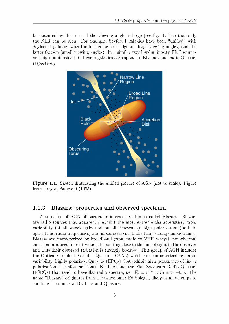
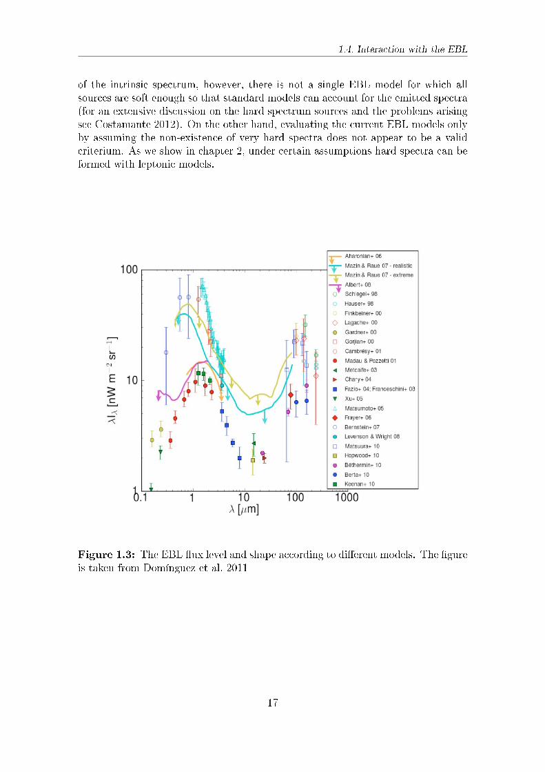
The EBL is the diuse light between the galaxies that comes from the stars. Itsorigin is extragalactic and so is expected to be isotropic on large scales. Its spectrumconsists of two bumps spreading from UV to far infrared (see g. 1.3). The rstcomponent peaks at wavelengths around ∼ 1µm and consists of emitted photonsfrom stars. Part of this light is absorbed by dust in the universe and is re-emittedin the infrared energy range, forming the second bump of the EBL which peaks at∼ 100µm.
Direct measurements of the EBL are very dicult because of strong foregroundemissions from the Milky Way and the Sun, especially the zodiacal light (Hauser &Dwek 2001). The exact ux level and shape are still a matter of debate as severalauthors have attempted to estimate the EBL with dierent techniques (for a recentreview see Domínguez et al. 2011 and references therein). There are basically threeapproaches to calculate the EBL: (a) Backward evolution which starts with thelocal galaxy population and scales it back in time, as a power-law in the redshift(e.g. Stecker & Scully 2008). Complementary to the aforementioned approachis the attempt to correct for the changing luminosity functions and SEDs withredshift and galaxy type (e.g. Kneiske et al., 2004; Franceschini et al., 2008). (b)Evolution directly observed and extrapolated based on a large set of multiwavelengthobservations (e.g. Domínguez et al. 2011) and (c) Forward evolution which beginswith initial cosmological conditions and evolves taking into account gas cooling indark matter halos, formation of galaxies including stars and AGN, feedback forthese phenomena, stellar evolution, emission, absorption and re-emission of lightfrom dust (e.g. Gilmore et al. 2012).
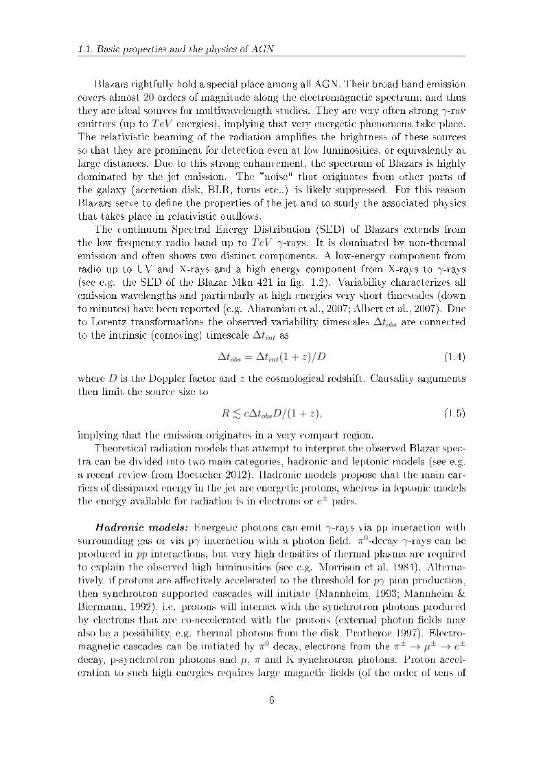
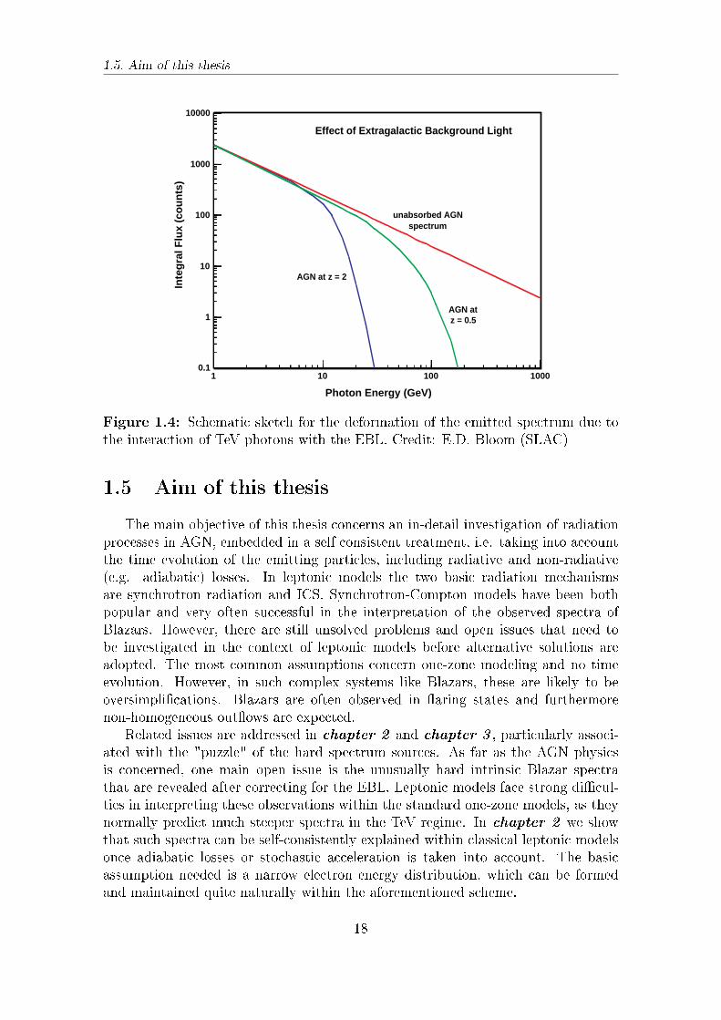
Among other, the EBL ux level and shape is highly relevant for understandingthe TeV emission from Blazars. The reason is that the TeV photons interact with theEBL photons, through the pair productions process, γγ → e+e− (see e.g. Gould &Schréder 1967). This mechanism results in the deformation of the intrinsic spectrumbecause the optical depth depends on the energy of the emitted photons. Thedeformation usually manifests as a softening, i.e. the observed photon index islarger than the one characterizing the intrinsic spectrum. This eect is more evidentfor more distant sources as the optical depth depends also on redshift (see g.1.4).Vice versa, when a soft photon TeV spectrum is observed, then the EBL correctedintrinsic spectrum may be harder. In principle this should not be a problem aswe don't know in detail the intrinsic Blazar spectra. However, in some cases theresulting spectra are very hard and can not be simply interpreted within standardleptonic models.
Obviously dierent models for estimating the EBL lead to dierent hardness
16
1.4. Interaction with the EBL
of the intrinsic spectrum, however, there is not a single EBL model for which allsources are soft enough so that standard models can account for the emitted spectra(for an extensive discussion on the hard spectrum sources and the problems arisingsee Costamante 2012). On the other hand, evaluating the current EBL models onlyby assuming the non-existence of very hard spectra does not appear to be a validcriterium. As we show in chapter 2, under certain assumptions hard spectra can beformed with leptonic models.
Figure 1.3: The EBL ux level and shape according to dierent models. The gureis taken from Domínguez et al. 2011
17
1.5. Aim of this thesis
unabsorbed AGN
AGN at z = 2
AGN atz = 0.5
Photon Energy (GeV)
Inte
gra
l Flu
x (c
ou
nts
)
spectrum
1 10 100 1000
10000
1000
100
10
1
0.1
Effect of Extragalactic Background Light
Figure 1.4: Schematic sketch for the deformation of the emitted spectrum due tothe interaction of TeV photons with the EBL. Credit: E.D. Bloom (SLAC)
1.5 Aim of this thesis
The main objective of this thesis concerns an in-detail investigation of radiationprocesses in AGN, embedded in a self consistent treatment, i.e. taking into accountthe time evolution of the emitting particles, including radiative and non-radiative(e.g. adiabatic) losses. In leptonic models the two basic radiation mechanismsare synchrotron radiation and ICS. Synchrotron-Compton models have been bothpopular and very often successful in the interpretation of the observed spectra ofBlazars. However, there are still unsolved problems and open issues that need tobe investigated in the context of leptonic models before alternative solutions areadopted. The most common assumptions concern one-zone modeling and no timeevolution. However, in such complex systems like Blazars, these are likely to beoversimplications. Blazars are often observed in aring states and furthermorenon-homogeneous outows are expected.
Related issues are addressed in chapter 2 and chapter 3 , particularly associ-ated with the "puzzle" of the hard spectrum sources. As far as the AGN physicsis concerned, one main open issue is the unusually hard intrinsic Blazar spectrathat are revealed after correcting for the EBL. Leptonic models face strong dicul-ties in interpreting these observations within the standard one-zone models, as theynormally predict much steeper spectra in the TeV regime. In chapter 2 we showthat such spectra can be self-consistently explained within classical leptonic modelsonce adiabatic losses or stochastic acceleration is taken into account. The basicassumption needed is a narrow electron energy distribution, which can be formedand maintained quite naturally within the aforementioned scheme.
18
1.5. Aim of this thesis
Apart from such self-consistent solutions we can also consider multi-zones forthe emitting region. A suitable combination of narrow distributions (as Maxwellian-type electron distributions) may then allow to interpret broader spectra too. Sucha scheme is capable of interpreting the broad spectrum of Mkn 501, equally or evenbetter than one smooth function which that is often examined. Furthermore, itallows to explain hard ares, like the one seen in Mkn 501 in 2009, once one (orfew) of the components become more energetic, either due to energy enhancementor change of orientation. This consideration is developed within a "leading" blobmodel which is explored in chapter 3 .
Obviously, though for so long and often studied, the leptonic models have moreto reveal concerning either one-zone models or more complex and possibly realisticcongurations. Even in on more basic level, namely regarding the radiation processesthemselves not embedded in a physical model that takes into account the evolution ofthe particles, there are still unexplored issues proved to be important regarding theinformation they oer for the physics of the source. One of these issues is the shape ofthe ICS spectrum close to the high energy cuto. This is analyzed in chapter 4 . Bydeveloping analytical approximations we directly link the exponential index as wellas the cuto energy of the emitted spectrum to the corresponding parameters of theparent electron distribution. These formulas allow us to extract crucial informationfor the electrons and their acceleration process in the source. Additionally, theyshed light onto other matters like a possible dependance on the magnetic eld fromthe spatial coordinates, or a more accurate extraction of the source parameters bythe comparison of the two peaks of the SED.
Apart from the emission mechanisms themselves, the observed spectrum is af-fected by the Doppler boosting due to the relativistic motion of the source. This isan essential ingredient for linking the observed ux in respect to the intrinsic ux.In chapter 5 we develop a solution of the photon transfer equation that allowsus to derive the dierent beaming patterns for various processes, i.e. synchrotronradiation, EC and SSC, in a concise way. In these calculation we extend the beam-ing pattern formulas to include generalized particle distributions, non-stationary,non-homogeneous and non-isotropic. This allows us to examine the interesting casein which the particles exhibit an energy-dependent anisotropy. Interestingly, theobserved spectrum does not only exhibit dierences as far as the total luminosityis concerned but it also appears harder depending on the angle of observation. Inprinciple, dropping some basic assumptions, like isotropy or homogeneity, can revealinteresting characteristics of the spectrum in respect to one-zone models. To someextend, the "leading" blob model is also a non-homogeneous model, that successfullyexplains spectral features that the standard models fail to interpret.
Concerning more realistic source congurations, it is particularly interesting toexamine non-homogeneous models where the relevant parameters vary in a contin-uous way. In chapter 6 we investigate an outow with transverse straticationassuming that particles are injected at the base of the jet, e.g. by DSA at a stand-ing shock. The bulk Lorentz factor, the magnetic eld, the particle number densityas well as the maximum energy are then assumed to vary across the jet. In a rststep we deal only with synchrotron radiation and we show that a variety of strati-
19
1.5. Aim of this thesis
cation consequences arise. For example, the spectrum appears dierent for dierentangles of observations. Furthermore special characteristics appear, like additionalspectral breaks, which are a direct evidence for non-homogeneous models. In total,even in this rst step, the observed (synchrotron) spectrum appears in some casessubstantially dierent from the spectra that corresponds to one-zone models.
20
Chapter 2
Formation of hard VHE γ-ray Blazar
spectra
The very high energy γ-ray spectra of some TeV Blazars, after being correctedfor absorption by the extragalactic background light (EBL), appear unusually hard.The interpretation of these hard intrinsic spectra poses challenges to conventionalacceleration and emission models. A time-dependent, self-consistent consideration iscrucial, because even extremely hard initial electron distributions can be signicantlydeformed due to radiative energy losses.
The main goal of this chapter is to examine whether very hard γ-ray spectracan be realized in time-dependent leptonic models. We investigate the parameterspace that allows for such a consideration both for synchrotron self-Compton (SSC)and external Compton (EC) scenarios. We demonstrate that very steep spectracan be avoided if adiabatic losses are taken into account. Another way to keepextremely hard electron distributions in the presence of losses is to assume stochasticacceleration models that naturally lead to steady-state relativistic, maxwellian-typedistributions.
We show that in either case leptonic models can reproduce TeV spectra as hardas Eγ dN/dEγ ∝ Eγ for SSC models and Eγ dN/dEγ ∝ E
1/3γ in an EC scenario.
Unfortunately this limits, to a large extend, the potential of extracting EBL fromgamma-ray observations of Blazars1.
2.1 The puzzle of hard γ-ray Blazar spectra
Though the standard one-zone SSC model, as well as the EC model, have beenthe bread and butter for interpreting the high energy spectrum of Blazars, some re-cent detections of VHE (Very High Energy) γ-rays from Blazars at redshift z ≥ 0.1(in particular, 1ES 1101-232 at z = 0.186 and 1ES 0229+200 at z = 0.139), posechallenges to the conventional leptonic interpretation. As discussed in detail inthe introduction, VHE γ-rays emitted by such distant objects arrive after signif-icant absorption caused by their interactions with extragalactic background light
1The results discussed in this chapter are based on Lefa et al. 2011
21
2.1. The puzzle of hard γ-ray Blazar spectra
(EBL) via the process γγ → e+e− (e.g., Gould & Schréder 1967). Reconstruction ofthe absorption-corrected intrinsic VHE γ-ray spectra based on state-of-the-art EBLmodels then yields unusually hard VHE source spectra, that are dicult to accountfor with the standard inverse Compton assumption.
The diculty lies in the eect that the radiation losses have on the emitting elec-tron distribution. Even if we (continuously) inject in the source the hardest possibledistribution, monoenergetic electrons, i.e. Q(γ) ∝ γδ(γ − γ∗), then synchrotron-type losses will result in the development of a power-law distribution of the formne(γ) ∝ γ−2, as one can directly see from solution of the kinetic equation in thesteady-state case
ne(γ) ∝1
γ
∫ ∞
γ
γδ(γ − γ∗)dγ ∝ γ−2Θ(γ∗ − γ). (2.1)
Note that hard VHE emission spectra can not be achieved even if one assumesthat particles cool due to ICS in the Klein-Nishina regime, in which case the steadystate particle distribution would indeed be harder due to the dierent energy depen-dance of the radiative losses (roughly speaking γKN ∝ ln 4γϵ/mc2, see e.g. Blumen-thal & Gould 1970). Nevertheless, this modication would have a strong impactonly on the synchrotron component of the spectrum, but not in the TeV energyband, because the particle distribution hardening is compensated by the reductionof the scattering eciency (Moderski et al. 2005). The characteristic γ−2 behavior ofthe electron distribution results in a photon spectrum of the form dNγ/dEγ ∝ E−Γ
γ ,with a photon index of Γ = 1.5. Sources with smaller photon indices have beenreported. Even the 1.5 photon index is dicult to achieve, as these sources peak atvery high energies where Klein-Nishina eects make the spectrum even steeper.
Current uncertainties on the EBL ux level and spectrum (cf. Primack et al.2011 for a recent review) introduce diculties in dening how hard the absorption-corrected source spectra are. However, for some sources the emitted spectra stilltend to be very hard, with an intrinsic photon index Γ ≤ 1.5, even when correctedfor low EBL ux levels (Aharonian et al., 2006, 2007a). One characteristic caseconcerns the distant (at z = 0.186) Blazar 1ES 1101-232, detected at VHE γ-rayenergies by the H.E.S.S. (High Energy Stereoscopic System) array of Cherenkovtelescopes (Aharonian et al., 2006, 2007a). When corrected for absorption by theEBL, the VHE γ-ray data result in very hard intrinsic spectra, with a peak in theSED above 3 TeV and a photon index Γ ≤ 1.5 (see e.g. g. 2.1). A similar behaviorhas also been detected in the BL Lacertae 1ES 0347-121 at z = 0.188 (Aharonian etal. 2007) whereas even more extreme values for the de-absorbed photon index werereported for the TeV Blazar 1ES 0229+200 at z=0.139 (Aharonian et al. 2007b).Though there is a non-negligible uncertainty in the EBL ux, the intrinsic spectra areunusually hard even when one considers the lowest levels of the EBL (Franceschiniet al. 2008). Other models predicting higher EBL ux lead to even harder photonindex close to 1 (e.g., Stecker & Scully 2008).
Interestingly, a recent analysis of Fermi LAT data for the nearby TeV Blazar Mkn501 indicates a hard γ-ray spectrum (Γ close to 1) at lower (10-200 GeV) energies(Neronov et al. 2011). Already in the original paper by the FERMI collaboration
22
2.2. Suggested solutions
-13
-12
-11
-10
log(
νFν
[erg
cm
-2 s
-1])
-13
-12
-11
1015
1017
1019
1021
1023
1025
1027
1028
ν [Hz]
log(
νFν
[erg
cm
-2 s
-1])
1ES 1101−232, March 5−16, 2005
1ES 1101−232, June 5−10, 2004
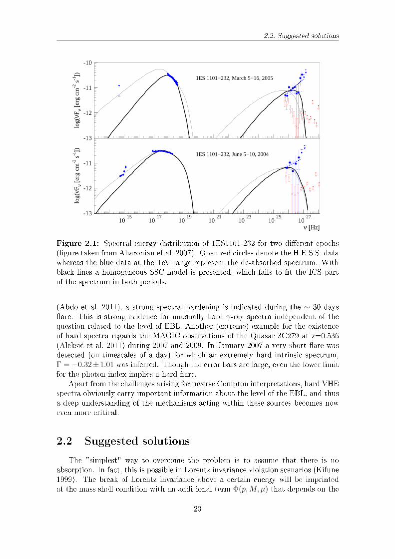
Figure 2.1: Spectral energy distribution of 1ES1101-232 for two dierent epochs(gure taken from Aharonian et al. 2007). Open red circles denote the H.E.S.S. datawhereas the blue data at the TeV range represent the de-absorbed spectrum. Withblack lines a homogeneous SSC model is presented, which fails to t the ICS partof the spectrum in both periods.
(Abdo et al. 2011), a strong spectral hardening is indicated during the ∼ 30 daysare. This is strong evidence for unusually hard γ-ray spectra independent of thequestion related to the level of EBL. Another (extreme) example for the existenceof hard spectra regards the MAGIC observations of the Quasar 3C279 at z=0.536(Aleksi¢ et al. 2011) during 2007 and 2009. In January 2007 a very short are wasdetected (on timescales of a day) for which an extremely hard intrinsic spectrum,Γ = −0.32±1.01 was inferred. Though the error bars are large, even the lower limitfor the photon index implies a hard are.
Apart from the challenges arising for inverse Compton interpretations, hard VHEspectra obviously carry important information about the level of the EBL, and thusa deep understanding of the mechanisms acting within these sources becomes noweven more critical.
2.2 Suggested solutions
The "simplest" way to overcome the problem is to assume that there is noabsorption. In fact, this is possible in Lorentz invariance violation scenarios (Kifune1999). The break of Lorentz invariance above a certain energy will be imprintedat the mass shell condition with an additional term Φ(p,M, µ) that depends on the
23
2.2. Suggested solutions
mass, the momentum and an arbitrary constant µ related to the model which isassumed for the symmetry breaking
ηijpipj = m2 + Φ(p,M, µ). (2.2)
The parameter M is a constant related to the scale at which the threshold anomalybecomes important. Here, ηij = (+,−,−,−) is the Minkowski metric and pi =(E,−p) the four-momentum. For the pair production process the above modiedrelation in combination with energy and momentum conservation alter the thresholdof the interaction, since
2ϵEγ(1− cos θ)− 2E2γΦ(p,M, µ) > 4m2, (2.3)
preventing the TeV photons to interact with the infrared photons of the EBL. Weshould note however that this eect is likely to be true only above 2 TeV (Stecker &Glashow 2001), whereas the hard spectra problem that we face in the case of distantBlazars is relevant to sub-TeV energies as well.
Another non standard mechanism to avoid severe absorption in the EBL hasbeen suggested by De Angelis et al. (2009) (see also Hooper & Serpico 2007) whoproposed that the γ-ray photon is mixing with a very light axion-like particle (ALP).These ALPs propagate unaected by the EBL, reducing in this way the mean freepath of the photons and thus allowing softer intrinsic spectra. However, this sce-nario requires the existence of exotic particles. To some extend a similar idea wassuggested by Essey et al. (2011) who assumed that the γ-rays from Blazars may bedominated by secondary γ-rays produced along the line of sight by the interactionsof cosmic-ray protons with background photons. While primary γ-rays emitted bythe Blazar are attenuated in their interactions with the EBL, cosmic rays with ener-gies 1016 - 1019 eV can cross cosmological distances and produce secondary γ-rays intheir interactions with the background photons. Protons are deected by magneticelds and thus this mechanism leads to upper bounds of the intergalactic magneticeld (see also Essey & Kusenko, 2010; Essey et al., 2010; Essey & Kusenko, 2012;Prosekin et al., 2012), which have not yet been conrmed by an alternative methodof magnetic eld estimation.
In more standard astrophysical scenarios, formation of hard γ-ray spectra couldbe related to production and absorption processes. Photon-photon absorption canresult in arbitrarily hard spectra provided that the γ-rays pass through a hot photongas with a narrow distribution such that Eγϵo ≫ mc2. In this case, due to thereduction of the cross-section the source becomes optically thick at lower energiesand thin to higher energies leading to formation of hard intrinsic spectra (Aharonianet al., 2008; Zacharopoulou et al., 2011). In such a scheme the primary TeV spectrumcould be due to synchrotron radiation of protons, whereas the low energy part isattributed to synchrotron radiation of secondary electrons.
Finally, if we relate the hard γ-ray spectra to the production process then thisimplies hard parent particle distribution. Outside standard leptonic models, a num-ber of alternative explanations have been explored in the literature. In analogy topulsar winds, Aharonian et al. (2002) have analyzed the implications of a cold ultra-relativistic outow that initially (close to the black hole) propagates at very high
24
2.3. Stationary SSC with an energetic electron distribution
velocities. In this case, upscattering of ambient photons can yield sharp pile-up fea-tures in the intrinsic source spectra. However, very high bulk Lorentz factors wouldbe required (Γb ∼ 107) and it seems not clear whether such a scenario can be appliedto Blazars. On the other hand, if Blazar jets would remain highly relativistic out tokpc-scales (Γb ∼ 10) and able to accelerate particles, a hard (slowly variable) VHEemission component could perhaps be produced by Compton up-scattering of CMB(Cosmic Microwave Background) photons (Böttcher et al. 2008).
Hard spectra can occur in standard leptonic scenarios as well. In order to producehard γ-ray spectra, hard electron energy distributions are required. Although stan-dard shock acceleration theories, both in the non-relativistic and relativistic regime,predict quite broad, n(Ee) ∝ E−2
e -type, electron energy distributions, there are non-conventional realizations which could give rise to very hard spectra (Derishev et al.,2003; Stecker et al., 2007). On a more phenomenological level, Katarzy«ski et al.(2006) have shown that the presence of an energetic power-law electron distributionwith a high value of the minimum cuto energy can lead to a hard TeV spectrum.In general, however, injection of a hard electron distribution is not a sucient con-dition as electrons are expected to quickly lose their energy due to radiative coolingand thereby develop a standard n(Ee) ∝ E−2
e form below the initial cuto energy. Inorder to avoid synchrotron cooling, one needs to assume unrealistically small valuesfor the magnetic eld (Tavecchio et al. 2009).
In this chapter we explore the conditions under which a narrow, energetic par-ticle distribution is able to successfully account for the hard VHE source spectra intime-dependent leptonic models. To this end, we examine dierent electron distribu-tions within the context of standard leptonic models, i.e. the one-zone SSC and theexternal Compton scenario. We show that time-dependent generalization includingadiabatic losses can self-consistently allow for hard TeV spectra to be maintained,without the need to avoid energy losses. As a second alternative, we discuss pile-up(Maxwellian-type) electron distributions that are formed in stochastic accelerationscenarios. These distributions are steady state solutions for which radiative (syn-chrotron or Thomson) losses are already included. They provide an interestingexplanation for very hard TeV components as their radiation spectra share manycharacteristics with the (hardest possible) mono-energetic distributions.
2.3 Stationary SSC with an energetic electron dis-
tribution
Within a stationary SSC approach, the hardest possible (extended) VHE spec-trum is approximately Fν ∝ ν1/3, where Fν = dF/dν is the spectral ux (dierentialux per frequency band). This has a simple explanation: As discussed in the intro-duction, the emitted synchrotron spectrum of a single electron with Lorentz factor γin a magnetic eld B, averaged over the particle's orbit, obeys j(ν, γ) ∝ G(x), whereG(x) is a dimensionless function with x = ν/νc and νc ≡ 3γ2eB sinα/(4πmec). Forx ≪ 1, the functional dependence of G(x) is well approximated by G(x) ∝ x1/3,while for x ≫ 1 one has G(x) ∝ x1/2e−x (e.g., Rybicki & Lightmann 1979). Hence,
25
2.3. Stationary SSC with an energetic electron distribution
at low frequencies ν ≪ νc, the synchrotron spectrum follows j(ν) ∝ ν1/3. Comptonupscattering of such a photon spectrum in the Thomson regime by a very energetic,narrow electron distribution will preserve this dependence and therefore yield a VHEspectral wing as hard as Fν ∝ ν1/3 as shown below.
2.3.1 Power-law electron distribution with high value of low-
energy cuto
A homogeneous SSC scenario with a high value for the low-energy cuto of thenon-thermal electron distribution has consequently been proposed by Katarzy«skiet al. (2006) in order to overcome the problem of the Klein-Nishina suppression ofthe cross-section at high energies and reproduce VHE spectra as hard as 1/3. Letus assume that the electron population follows a power-law distribution of index pbetween the low- and high-energy cutos
N ′e(γ
′) = K ′eγ
′−p, γ′min < γ′ < γ′
max , (2.4)
as often used in modeling the Blazar spectra. Here, prime quantities refer to theblob rest frame and unprimed to the observer's frame. Taking relativistic Dopplerboosting (D) into account, the observed synchrotron ux from an optically thinsource at distance dL is given by the integral of N ′
e(γ′)dγ′ times the single particle
emissivity j′(ν ′, γ′) over the volume element and all energies γ′ (e.g., Begelman etal. 1984), i.e.
F synν =
D3
d2L
∫V ′
∫γ′j′(ν ′, γ′)N ′
e(γ′)dγ′dV ′ . (2.5)
The above expression yields the common power-law of index α = (p− 1)/2 betweenthe frequency limits νmin ∝ D(Bγ2
min) and νmax ∝ D(Bγ2max). Below and above
those limits, the electrons with energy around the minimum and maximum cutodominates and thus the spectrum approximately exhibits a slope Fν ∝ ν1/3 forν < νmin, and an exponential cuto for ν > νmax, i.e.
F synν ∝
ν1/3, ν ≪ νminν− p−1
2 , νmin ≤ ν ≤ νmaxν1/2e−ν , ν ≫ νmax
(2.6)
The hard 1/3-slope appears in the VHE range of EC γ-rays when the synchrotronphotons are up-scattered to higher energies by the electron population given byequation (2.4) with a high γmin and provided that the Thomson regime applies.Obviously, in the Klein-Nishina regime it will be signicantly steeper. In any case,however, there exists a characteristic energy below which the Compton spectrummimics the behavior of the synchrotron spectrum Fν ∝ ν1/3.
Note that the ICS spectrum of a monochromatic photon eld by monoenergeticelectrons approximately follows Fν ∝ ν at low energies (cf. Blumenthal & Gould1970). Thus, any photon eld which is softer (atter) than Fν ∝ ν will dominatethe lower-energy part of the up-scattered emission and thus, in the standard SSC
26
2.3. Stationary SSC with an energetic electron distribution
scenario the 1/3-VHE slope (the 4/3-slope in the νFν representation) is the hardestthat can be achieved.
An exception to this may occur if the magnetic eld in the source would be fullyturbulent with zero mean component. In such a case, the low-frequency part of thesynchrotron spectrum could be harder than Fν ∝ ν1/3 (Medvedev, 2006; Derishevet al., 2007; Reville & Kirk, 2010), which will be reected to low energy part of theCompton component.
The "critical Compton energy" is usually ϵmin ≃ Dγ2min(bγ
2min), where b ≡
(B/Bcr)mec2, Bcr = m2
ec3/(e~), except for the case of deep Klein-Nishina (KN)
regime, i.e., when up-scattering of the minimum synchrotron photons by the min-imum energy electrons occurs in the KN regime so that 4
3bγ3
min > 1. If the latterapplies, then the corresponding energy below which one can see the hard 1/3-slope is,as expected, γminmec
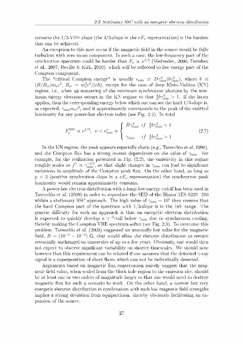
2, and it approximately corresponds to the peak of the emittedluminosity for any power-law electron index (see Fig. 2.2). In total
F SSCν ∝ ν1/3, ν < νcmin ∝
Bγ3
min if 43bγ3min < 1
γmin if 43bγ3min > 1
(2.7)
In the KN regime, the peak appears especially sharp (e.g., Tavecchio et al. 1998),and the Compton ux has a strong inverse dependence on the value of γmin. Forexample, for the realization presented in Fig. (2.2), the emissivity in this regimeroughly scales as jC ∝ γ−2.5
min , so that slight changes in γmin can lead to signicantvariations in amplitude of the Compton peak ux. On the other hand, as long asp < 3 (positive synchrotron slope in a νFν representation) the synchrotron peakluminosity would remain approximately constant.
A power-law electron distribution with a large low-energy cuto has been used inTavecchio et al. (2009) in order to reproduce the SED of the Blazar 1ES 0229+200within a stationary SSC approach. The high value of γmin ∼ 105 then ensures thatthe hard Compton part of the spectrum with 1/3-slope is in the TeV range. Thegeneric diculty for such an approach is that an energetic electron distributionis expected to quickly develop a γ−2-tail below γmin due to synchrotron cooling,thereby making the Compton VHE spectrum softer (see Fig. 2.3). To overcome thisproblem, Tavecchio et al. (2009) suggested an unusually low value for the magneticeld, B ∼ (10−4 − 10−3) G, that would allow the electron distribution to remainessentially unchanged on timescales of up to a few years. Obviously, one would thennot expect to observe signicant variability on shorter timescales. We should notehowever that this requirement can be relaxed if one assumes that the detected γ-raysignal is a superposition of short ares which can not be individually detected.
Arguments based on magnetic ux conservation naively suggest that the mag-netic eld value, when scaled from the black hole region to the emission site, shouldbe at least one or two orders of magnitude larger so that one would need to destroymagnetic ux for such a scenario to work. On the other hand, a narrow but veryenergetic electron distribution in combination with such low magnetic eld strengthsimplies a strong deviation from equipartition, thereby obviously facilitating an ex-pansion of the source.
27
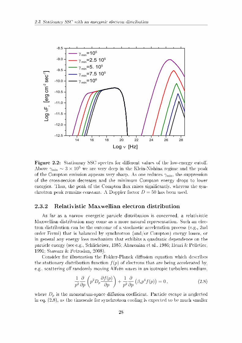
2.3. Stationary SSC with an energetic electron distribution
14 16 18 20 22 24 26 28-12.5
-12.0
-11.5
-11.0
-10.5
-10.0
-9.5
-9.0
-8.5Lo
g F
[er
g cm
-2 s
ec-1]
Log [Hz]
min=105
min=2.5 105
min=5. 105
min=7.5 105
min=106
Figure 2.2: Stationary SSC spectra for dierent values of the low-energy cuto.Above γmin ∼ 3 × 10⁵ we are very deep in the Klein-Nishina regime and the peakof the Compton emission appears very sharp. As one reduces γmin, the suppressionof the cross-section decreases and the minimum Compton energy drops to lowerenergies. Thus, the peak of the Compton ux raises signicantly, whereas the syn-chrotron peak remains constant. A Doppler factor D = 50 has been used.
2.3.2 Relativistic Maxwellian electron distribution
As far as a narrow energetic particle distribution is concerned, a relativisticMaxwellian distribution may come as a more natural representation. Such an elec-tron distribution can be the outcome of a stochastic acceleration process (e.g., 2ndorder Fermi) that is balanced by synchrotron (and/or Compton) energy losses, orin general any energy loss mechanism that exhibits a quadratic dependence on theparticle energy (see e.g., Schlickeiser, 1985; Aharonian et al., 1986; Henri & Pelletier,1991; Stawarz & Petrosian, 2008).
Consider for illustration the Fokker-Planck diusion equation which describesthe stationary distribution function f(p) of electrons that are being accelerated by,e.g., scattering o randomly moving Alfvén waves in an isotropic turbulent medium,
1
p2∂
∂p
(p2Dp
∂f(p)
∂p
)+
1
p2∂
∂p
(βsp
4f(p))= 0 , (2.8)
where Dp is the momentum-space diusion coecient. Particle escape is neglectedin eq. (2.8), as the timescale for synchrotron cooling is expected to be much smaller
28
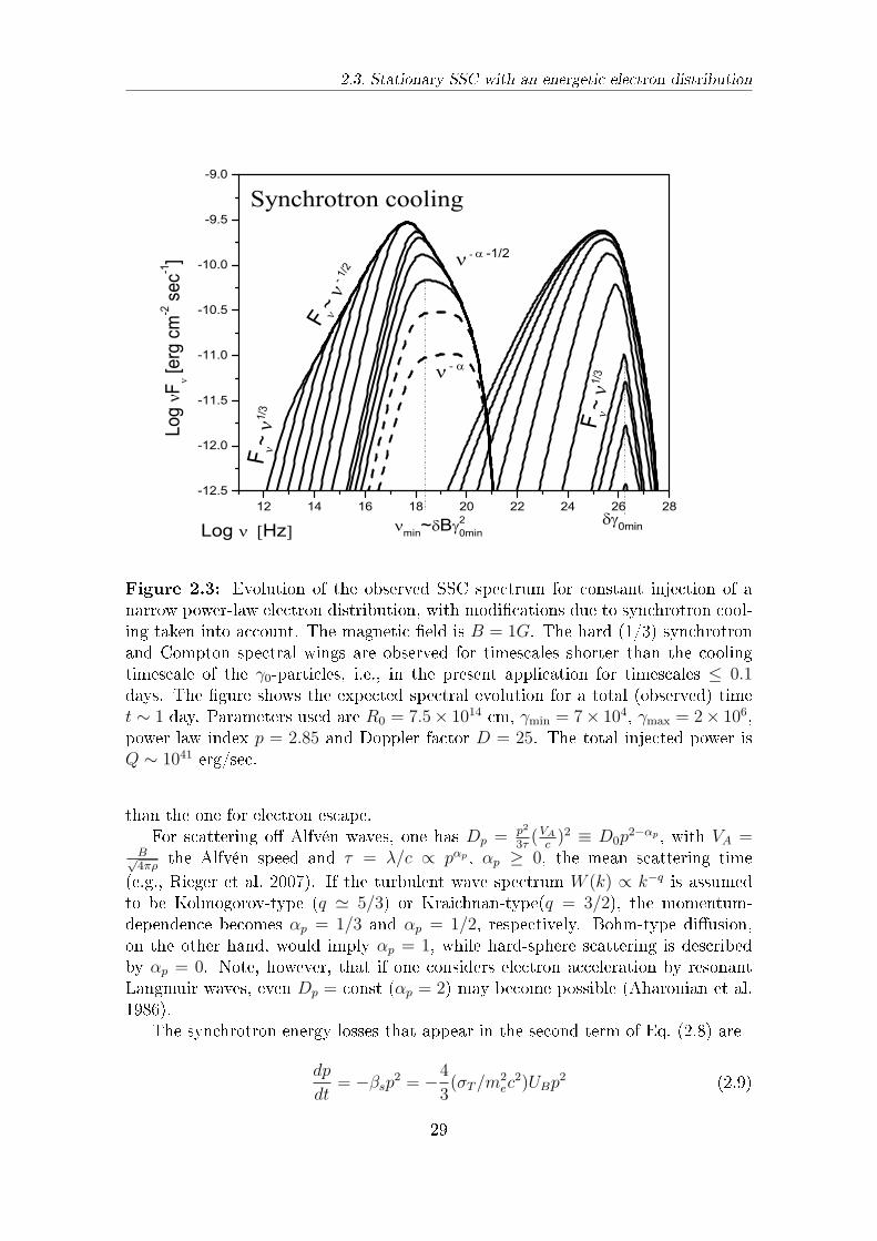
2.3. Stationary SSC with an energetic electron distribution
12 14 16 18 20 22 24 26 28-12.5
-12.0
-11.5
-11.0
-10.5
-10.0
-9.5
-9.0
Synchrotron cooling
F~
1/3
F~
1/3 -
- -1/2
F~
- 1/2
min~ B 20min 0min
Log
F [e
rg c
m-2 s
ec-1]
Log Hz
Figure 2.3: Evolution of the observed SSC spectrum for constant injection of anarrow power-law electron distribution, with modications due to synchrotron cool-ing taken into account. The magnetic eld is B = 1G. The hard (1/3) synchrotronand Compton spectral wings are observed for timescales shorter than the coolingtimescale of the γ0-particles, i.e., in the present application for timescales ≤ 0.1days. The gure shows the expected spectral evolution for a total (observed) timet ∼ 1 day. Parameters used are R0 = 7.5× 1014 cm, γmin = 7× 10⁴, γmax = 2× 10⁶,power law index p = 2.85 and Doppler factor D = 25. The total injected power isQ ∼ 1041 erg/sec.
than the one for electron escape.For scattering o Alfvén waves, one has Dp = p2
3τ(VAc)2 ≡ D0p
2−αp , with VA =B√4πρ
the Alfvén speed and τ = λ/c ∝ pαp , αp ≥ 0, the mean scattering time(e.g., Rieger et al. 2007). If the turbulent wave spectrum W (k) ∝ k−q is assumedto be Kolmogorov-type (q ≃ 5/3) or Kraichnan-type(q = 3/2), the momentum-dependence becomes αp = 1/3 and αp = 1/2, respectively. Bohm-type diusion,on the other hand, would imply αp = 1, while hard-sphere scattering is describedby αp = 0. Note, however, that if one considers electron acceleration by resonantLangmuir waves, even Dp = const (αp = 2) may become possible (Aharonian et al.1986).
The synchrotron energy losses that appear in the second term of Eq. (2.8) are
dp
dt= −βsp
2 = −4
3(σT/m
2ec
2)UBp2 (2.9)
29
2.3. Stationary SSC with an energetic electron distribution
In the γ-parameter space, the solution of Eq. (2.8) yields a relativistic Maxwell-like energy distribution,
dNe(γ)/dγ = f(γ) = Aγ2e−(γγc)1+αp
, (2.10)
(αp = −1) with
γc =
([1 + αp]D0
βs
)1/(1+αp)
(mec2)−1 , (2.11)
and constant A to be dened by the initial conditions. Note that this is a steady-state solution including radiative losses and there is no need to invoke extreme valuesfor the magnetic eld. The critical Lorentz factor γc approximately corresponds tothe energy at which acceleration on timescale
tacc =3
4− αp
(c
VA
)2
τ (2.12)
is balanced by (synchrotron) cooling on timescale tcool = 1/[βsp]. Depending onthe choice of parameters, a relatively large range of values for γc is possible andthus, cuto energies of the order of γc ∼ 105 may well be achieved. Consider, forexample, Bohm-type diusion with τ = ηrg/c, rg = γmec
2/(eB) the electron gyro-radius and η ≥ 1. Using tacc = tcool, the maximum electron Lorentz factor becomesγc ≃ 106 (vA/0.01c) (1 G/B)1/2η−1/2.
The synchrotron spectrum that arises from a Maxwell-like electron distribution isdominated by the emission of electrons with γc (Fig. 2.4). It exhibits the character-istic 1/3-slope up to the corresponding "synchrotron cuto frequency" hνsyn
c ∼ Dbγ2c
where b = B/Bcr and Bcr = m2c3/e~. Thus the Compton spectrum is very similarto the one resulting from a narrow power-law if one chooses a value for the cuto en-ergy close to the minimum electron energy of the power-law distribution. The peakof the Compton ux then contains information for the cuto energy as νcpeak ∝ γc.
Note that for an electron distribution of the form of eq. (3.1) that exhibits anexponential cuto ∝ exp[−(γ/γc)
β], the corresponding cuto in the synchrotronspectrum appears much smoother, ∝ exp[−(ν/ν∗)
β/(β+2)] (Fritz, 1989; Zirakashvili& Aharonian, 2007). The position of the synchrotron peak ux, νp, is then alsodependent on β, and one can show that for β = 1 (or αp = 0 in the previousnotation) an important factor ∼ 10 arises, so that νp = 9.5νc, whereas for β = 3the synchrotron peak corresponds approximately to the electron cuto as νp = 1.2νc(e.g., Fig. 2.4). For an extended discussion on the cuto energies for the synchrotronand ICS spectrum see chapter 4.
30
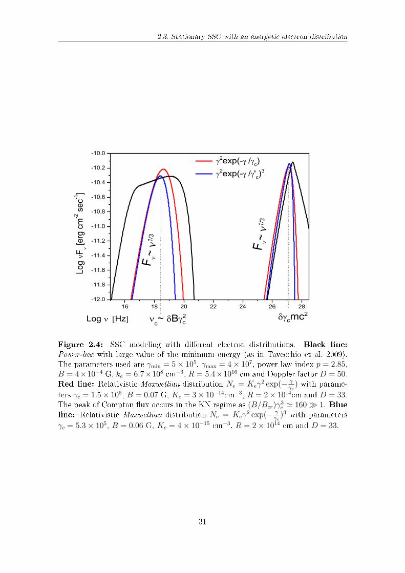
2.3. Stationary SSC with an energetic electron distribution
16 18 20 22 24 26 28-12.0
-11.8
-11.6
-11.4
-11.2
-11.0
-10.8
-10.6
-10.4
-10.2
-10.0
cmc2c~ B 2
c
F~
1/3
F~
1/3
Log
F [e
rg c
m-2 s
ec-1]
Log Hz
2exp(- / c) 2exp(- / 'c)
3
Figure 2.4: SSC modeling with dierent electron distributions. Black line:
Power-law with large value of the minimum energy (as in Tavecchio et al. 2009).The parameters used are γmin = 5× 10⁵, γmax = 4× 10⁷, power law index p = 2.85,B = 4×10⁻⁴ G, ke = 6.7×108 cm−3, R = 5.4×1016 cm and Doppler factor D = 50.Red line: Relativistic Maxwellian distribution Ne = Keγ
2 exp(− γγc) with parame-
ters γc = 1.5× 10⁵, B = 0.07 G, Ke = 3× 10⁻¹⁴cm−3, R = 2× 1014cm and D = 33.The peak of Compton ux occurs in the KN regime as (B/Bcr)γ
3c ≃ 160 ≫ 1. Blue
line: Relativistic Maxwellian distribution Ne = Keγ2 exp(− γ
γc)3 with parameters
γc = 5.3× 10⁵, B = 0.06 G, Ke = 4× 10⁻¹⁵ cm−3, R = 2× 1014 cm and D = 33.
31
2.4. Time dependent case - expansion of the source
2.4 Time dependent case - expansion of the source
Expansion of the source could change the conclusions drawn above. In particular,if one assumes a very low magnetic eld such that synchrotron losses are negligible,then adiabatic losses may become important and alter the electron distribution. Inthis section, we examine the behavior of the system for a power-law electron distri-bution with a high value of the low-energy cuto discussed above. For simplicity,we consider a spherical source that expands with a constant velocity u,
R(t) = R0 + u(t− t0) . (2.13)
The relativistic electron population will be aected by synchrotron losses,
Psyn = −dγ
dt=
σTB(t)2γ2
6πmec, (2.14)
and by adiabatic losses (e.g., Longair 1982),
Pad = −dγ
dt≃ 1
3
V
Vγ =
R(t)
R(t)γ =
u
R(t)γ . (2.15)
As the emission region expands, the magnetic eld decreases. We consider a scalingB ∝ (1/R)m ∝ (1/t)m with 1 ≤ m ≤ 2 to study the evolution of the system.The limiting value m = 2 corresponds to conservation of magnetic ux for thelongitudinal component, whereas m = 1 holds for the perpendicular component.(Note that for m = 1 the ratio of the electrons' energy density to the magnetic eldenergy density remains constant). Which energy loss process then determines theelectron behavior depends mainly on the magnetic eld strength and the size of thesource. A simple comparison of the above relations shows that when Pad > Psyn,i.e.,
B(t)2R(t) <6πmec
2
σT
(uc
) 1
γ= 2.3× 10¹⁹
(uc
) 1
γ(2.16)
adiabatic losses dominate over radiative losses. For example, if one considers expan-sion at speed u ∼ c and an initial source dimension R0 ∼ 1014 cm, then for energiesbelow γ ∼ 107 the magnetic eld can be as large as B ∼ 0.1 G and for energies lessthan γ ∼ 105 the adiabatic losses are still dominant for a value of B ∼ 1 G. If theexpansion of the source would not aect the hard slope at TeV energies, this couldthus allow for a relaxation of the values used for SSC modeling of the source. Inorder to investigate this scenario in more detail, one needs to solve the electrons'kinetic equation
∂Ne(γ, t)
∂t=
∂
∂γ(PadNe(γ, t))−
Ne(γ, t)
τe+Q(γ, t) , (2.17)
where τe is the characteristic escape time and Ne the dierential electron number.For simplicity, we neglect the escape term (τe → ∞), assuming that the sourcesexpands with relativistic speeds u ∼ (0.1− 1)c. For a constant expansion rate and
32
2.4. Time dependent case - expansion of the source
continuous injection with rate Q(γ, t) → Q(γ,R), we can replace the time variablet by the source dimension R. Then, the general solution of the kinetic equation (eq.(30) from Atoyan & Aharonian 1999) for the case of dominance of adiabatic lossesis reduced to
Ne(γ,R) =R
R0
N0
(R
R0
γ
)+
1
u
∫ R
R0
R
rQ
(R
rγ, r
)dr , (2.18)
where the rst term corresponds to the initial conditions, the contributions of whichquickly disappears, and the second term relates to the continuous injection of rela-tivistic electrons. R0 is the source dimension at the initial time t0.
We consider zero initial conditions (N0 = 0) and power-law injection of relativis-tic particles at constant rate
Q(γ,R) = Q0γ−p1 Θ(γ − γ0,min)Θ(γ0,max − γ)Θ(R−R0) , (2.19)
where Θ denotes the unit step function
Θ(x− x0) =
1, x > x0
0, x < x0 ,(2.20)
p1 > 0 is the momentum index and R0 the radius at which injection starts. Atradius R, electrons with initial cuto energies γ0,min and γ0,max will have energiesγR,min and γR,max, respectively, as they evolve according to Eq. (2.15), i.e. we have
γR = γ0R0
R(t)∝ 1
t. (2.21)
From the properties of the step-function, the integral can be written as
Ne(γ,R) =Q0γ
−p1
u
∫ R
R0
(R
r
)1−p1Θ
(r − Rγ
γ0,max
)Θ
(Rγ
γ0,min− r
)dr
=Q0γ
−p1
u
∫ min[R, Rγγ0,min
]
max[R0,Rγ
γ0,max]
(R
r
)1−p1dr (2.22)
The comparison of the values for the lower and maximum limits of integration willresult in the dierent branches of the solution, whereas ensuring that the two limitsdo not overlap reveals a critical radius R∗ = R0γ0,max/γ0,min at which γR,max, i.e. theenergy of an electron with initial injected energy γ0,max at R, becomes less than theinitial γ0,min. The following two cases can be distinguished:
For R < R∗, or equivalently as long as γR,max > γ0,min, we have
N(γ,R) =Q0
p1uR
γ−p1[1−
(γ
γ0,max
)p1], γR,max < γ < γ0,max
γ−p1[1−
(R0
R
)p1], γ0,min < γ < γR,max
γ−p10,min −
(RγR0
)−p1, γR,min < γ < γ0,min
(2.23)
33
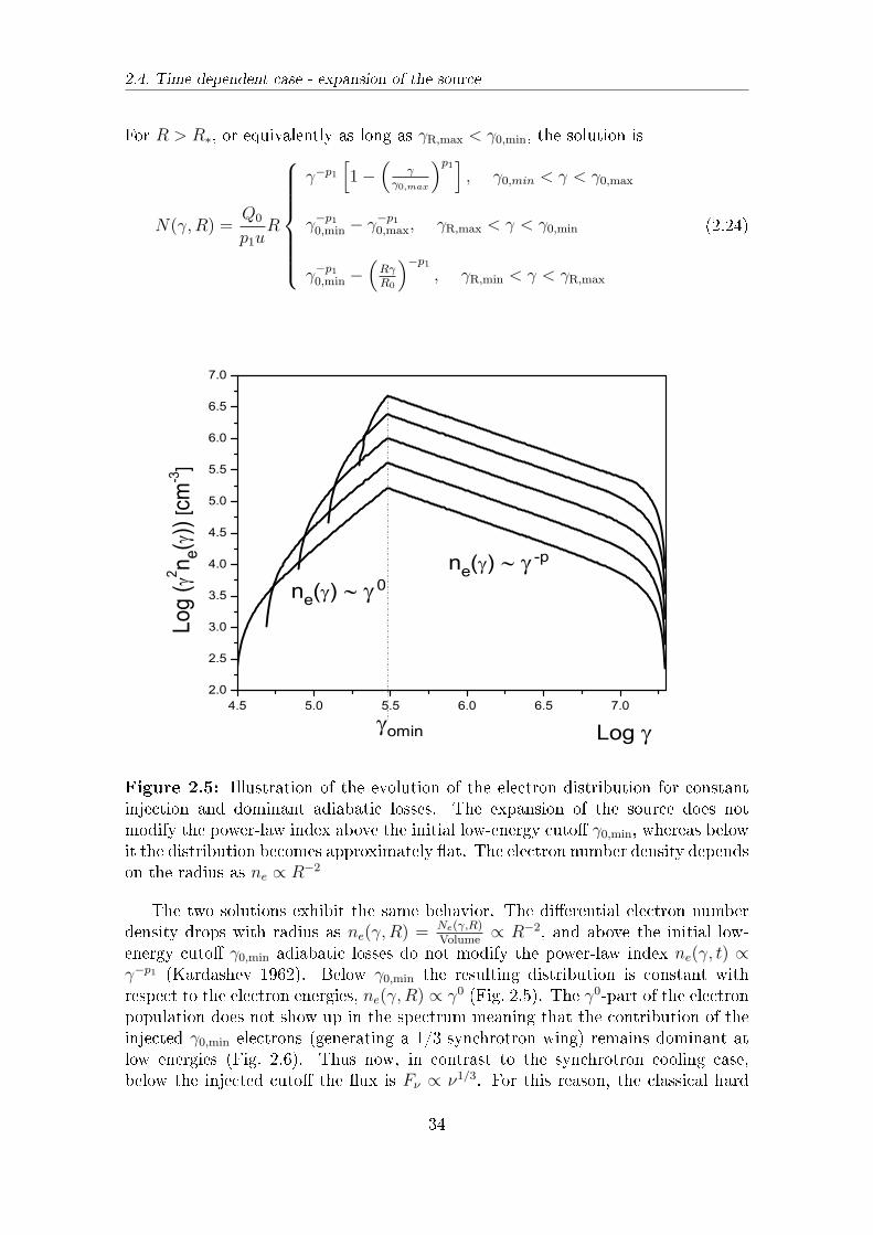
2.4. Time dependent case - expansion of the source
For R > R∗, or equivalently as long as γR,max < γ0,min, the solution is
N(γ,R) =Q0
p1uR
γ−p1[1−
(γ
γ0,max
)p1], γ0,min < γ < γ0,max
γ−p10,min − γ−p1
0,max, γR,max < γ < γ0,min
γ−p10,min −
(RγR0
)−p1, γR,min < γ < γR,max
(2.24)
4.5 5.0 5.5 6.0 6.5 7.02.0
2.5
3.0
3.5
4.0
4.5
5.0
5.5
6.0
6.5
7.0
ne( ) 0ne( ) -p
omin
Log
(2 n e())
[cm-3
]
Log
Figure 2.5: Illustration of the evolution of the electron distribution for constantinjection and dominant adiabatic losses. The expansion of the source does notmodify the power-law index above the initial low-energy cuto γ0,min, whereas belowit the distribution becomes approximately at. The electron number density dependson the radius as ne ∝ R−2
The two solutions exhibit the same behavior. The dierential electron numberdensity drops with radius as ne(γ,R) = Ne(γ,R)
Volume∝ R−2, and above the initial low-
energy cuto γ0,min adiabatic losses do not modify the power-law index ne(γ, t) ∝γ−p1 (Kardashev 1962). Below γ0,min the resulting distribution is constant withrespect to the electron energies, ne(γ,R) ∝ γ0 (Fig. 2.5). The γ0-part of the electronpopulation does not show up in the spectrum meaning that the contribution of theinjected γ0,min electrons (generating a 1/3-synchrotron wing) remains dominant atlow energies (Fig. 2.6). Thus now, in contrast to the synchrotron cooling case,below the injected cuto the ux is Fν ∝ ν1/3. For this reason, the classical hard
34
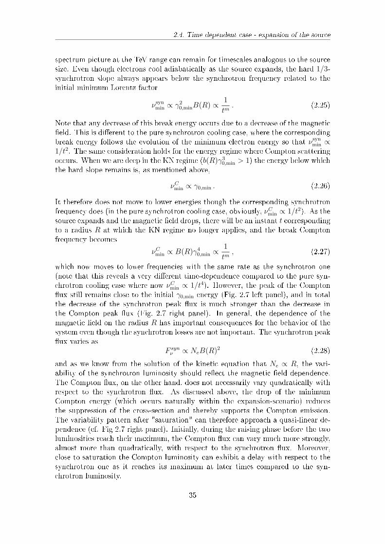
2.4. Time dependent case - expansion of the source
spectrum picture at the TeV range can remain for timescales analogous to the sourcesize. Even though electrons cool adiabatically as the source expands, the hard 1/3-synchrotron slope always appears below the synchrotron frequency related to theinitial minimum Lorentz factor
νsynmin ∝ γ2
0,minB(R) ∝ 1
tm. (2.25)
Note that any decrease of this break energy occurs due to a decrease of the magneticeld. This is dierent to the pure synchrotron cooling case, where the correspondingbreak energy follows the evolution of the minimum electron energy so that νsyn
min ∝1/t2. The same consideration holds for the energy regime where Compton scatteringoccurs. When we are deep in the KN regime (b(R)γ3
0,min > 1) the energy below whichthe hard slope remains is, as mentioned above,
νCmin ∝ γ0,min . (2.26)
It therefore does not move to lower energies though the corresponding synchrotronfrequency does (in the pure synchrotron cooling case, obviously, νCmin ∝ 1/t2). As thesource expands and the magnetic eld drops, there will be an instant t correspondingto a radius R at which the KN regime no longer applies, and the break Comptonfrequency becomes
νCmin ∝ B(R)γ40,min ∝ 1
tm, (2.27)
which now moves to lower frequencies with the same rate as the synchrotron one(note that this reveals a very dierent time-dependence compared to the pure syn-chrotron cooling case where now νCmin ∝ 1/t4). However, the peak of the Comptonux still remains close to the initial γ0,min energy (Fig. 2.7 left panel), and in totalthe decrease of the synchrotron peak ux is much stronger than the decrease inthe Compton peak ux (Fig. 2.7 right panel). In general, the dependence of themagnetic eld on the radius R has important consequences for the behavior of thesystem even though the synchrotron losses are not important. The synchrotron peakux varies as
F synν ∝ NeB(R)2 (2.28)
and as we know from the solution of the kinetic equation that Ne ∝ R, the vari-ability of the synchrotron luminosity should reect the magnetic eld dependence.The Compton ux, on the other hand, does not necessarily vary quadratically withrespect to the synchrotron ux. As discussed above, the drop of the minimumCompton energy (which occurs naturally within the expansion-scenario) reducesthe suppression of the cross-section and thereby supports the Compton emission.The variability pattern after "saturation" can therefore approach a quasi-linear de-pendence (cf. Fig 2.7 right panel). Initially, during the raising phase before the twoluminosities reach their maximum, the Compton ux can vary much more strongly,almost more than quadratically, with respect to the synchrotron ux. Moreover,close to saturation the Compton luminosity can exhibit a delay with respect to thesynchrotron one as it reaches its maximum at later times compared to the syn-chrotron luminosity.
35
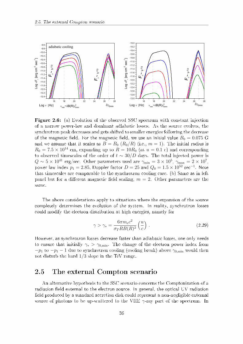
2.5. The external Compton scenario
16 18 20 22 24 26 28
-12.4
-12.2
-12.0
-11.8
-11.6
-11.4
-11.2
-11.0
-10.8
-10.6
-10.4
-10.2
-10.0
-9.8
-9.6
F~
1/3
0minmin~ B(R) 20min
F~
1/3
adiabatic cooling
Log
F [e
rg c
m-2 s
ec-1]
Log Hz16 18 20 22 24 26 28
-13.0
-12.8
-12.6
-12.4
-12.2
-12.0
-11.8
-11.6
-11.4
-11.2
-11.0
-10.8
-10.6
-10.4
-10.2
-10.0
0minmin~ B(R) 2
0min
F~
1/3
F~
1/3
Log
F [e
rg c
m-2 s
ec-1]
Log Hz
Figure 2.6: (a) Evolution of the observed SSC spectrum with constant injectionof a narrow power-law and dominant adiabatic losses. As the source evolves, thesynchrotron peak decreases and gets shifted to smaller energies following the decreaseof the magnetic eld. For the magnetic eld, we use an initial value B0 = 0.075 Gand we assume that it scales as B = B0 (R0/R) (i.e., m = 1). The initial radius isR0 = 7.5 × 1014 cm, expanding up to R = 10R0 (at u = 0.1 c) and correspondingto observed timescales of the order of t ∼ 30/D days. The total injected power isQ ∼ 5 × 1041 erg/sec. Other parameters used are γmin = 3 × 10⁵, γmax = 2 × 10⁷,power law index p1 = 2.85, Doppler factor D = 25 and Q0 = 1.5× 1052 sec−1. Notethat timescales are comparable to the synchrotron cooling case. (b) Same as in leftpanel but for a dierent magnetic eld scaling, m = 2. Other parameters are thesame.
The above considerations apply to situations where the expansion of the sourcecompletely determines the evolution of the system. In reality, synchrotron lossescould modify the electron distribution at high energies, namely for
γ > γ∗ =6πmec
2
σTRB(R)2
(uc
). (2.29)
However, as synchrotron losses decrease faster than adiabatic losses, one only needsto ensure that initially γ∗ > γ0,min. The change of the electron power index from−p1 to −p1 − 1 due to synchrotron cooling (cooling break) above γ0,min would thennot disturb the hard 1/3 slope in the TeV range.
2.5 The external Compton scenario
An alternative hypothesis to the SSC scenario concerns the Comptonization of aradiation eld external to the electron source. In general, the optical-UV radiationeld produced by a standard accretion disk could represent a non-negligible externalsource of photons to be up-scattered to the VHE γ-ray part of the spectrum. In
36
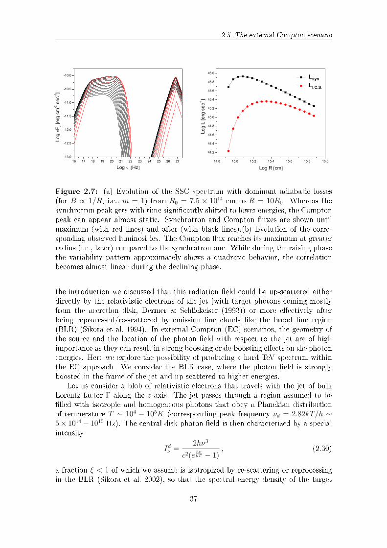
2.5. The external Compton scenario
16 17 18 19 20 21 22 23 24 25 26 27-13.0
-12.5
-12.0
-11.5
-11.0
-10.5
-10.0
Log
F [e
rg c
m-2 s
ec-1]
Log Hz14.8 15.0 15.2 15.4 15.6 15.8 16.0
44.2
44.4
44.6
44.8
45.0
45.2
45.4
45.6
45.8
46.0
Log
L [e
rg s
ec-1]
Log R cm
Lsyn LI.C.S.
Figure 2.7: (a) Evolution of the SSC spectrum with dominant adiabatic losses(for B ∝ 1/R, i.e., m = 1) from R0 = 7.5 × 1014 cm to R = 10R0. Whereas thesynchrotron peak gets with time signicantly shifted to lower energies, the Comptonpeak can appear almost static. Synchrotron and Compton uxes are shown untilmaximum (with red lines) and after (with black lines).(b) Evolution of the corre-sponding observed luminosities. The Compton ux reaches its maximum at greaterradius (i.e., later) compared to the synchrotron one. While during the raising phasethe variability pattern approximately shows a quadratic behavior, the correlationbecomes almost linear during the declining phase.
the introduction we discussed that this radiation eld could be up-scattered eitherdirectly by the relativistic electrons of the jet (with target photons coming mostlyfrom the accretion disk, Dermer & Schlickeiser (1993)) or more eectively afterbeing reprocessed/re-scattered by emission line clouds like the broad line region(BLR) (Sikora et al. 1994). In external Compton (EC) scenarios, the geometry ofthe source and the location of the photon eld with respect to the jet are of highimportance as they can result in strong boosting or de-boosting eects on the photonenergies. Here we explore the possibility of producing a hard TeV spectrum withinthe EC approach. We consider the BLR case, where the photon eld is stronglyboosted in the frame of the jet and up-scattered to higher energies.
Let us consider a blob of relativistic electrons that travels with the jet of bulkLorentz factor Γ along the z-axis. The jet passes through a region assumed to belled with isotropic and homogeneous photons that obey a Planckian distributionof temperature T ∼ 104 − 105K (corresponding peak frequency νd = 2.82kT/h ∼5× 10¹⁴ − 1015 Hz). The central disk photon eld is then characterized by a specialintensity
Idν =2hν3
c2(ehνkT − 1)
, (2.30)
a fraction ξ < 1 of which we assume is isotropized by re-scattering or reprocessingin the BLR (Sikora et al. 2002), so that the spectral energy density of the target
37
2.6. Summary and application to 1ES 0229+200
photon eld is
UBLRν =
ξLdν4πcr2BLR
, (2.31)
where Ldν = 4π2r2dIdν is the spectral luminosity of the disk and where we take rd ∼ rs
for the disk radius.In order to take anisotropic eects into account, we transform the electron distri-
bution from the comoving blob frame K ′ to the rest frame K of the external photoneld, which in our case coincides with the observer's frame (Georganopoulos et al.2001). Electrons are assumed to be isotropic in the blob frame K ′. In the photonframe K they exhibit a strong dependence on the angle θ, which is the observer'sangle. As the up-scattered photons travel inside a cone of opening angle 1/γ, we canmake the approximation that they follow the direction of the electrons. The anglebetween the electron momentum and the bulk velocity of the jet coincides with theobserver's angle. The observer practically sees radiation only from electrons that inthe photon frame are directed towards him. The observed ux then is
Fϵγ =D3
d2L
∫N ′e(E
D) W (E, ϵph, ϵγ) nph(ϵph)dE dϵph (2.32)
where Ne(E) denotes the dierential number of electrons per energy per solid angle,and W = Eγ
dNdtdEγ
is the scattered photon spectrum per electron (Blumenthal &Gould 1970). The unprimed quantities refer to the external photon eld frame withnumber density nph(ϵph) and the primed ones to the blob rest frame. Eq. 2.32 isderived analytically in chapter 5.
We show the calculated Compton spectrum for a Maxwellian electron distribu-tion in Fig. 2.8. The resulting TeV slope appears even harder than in the SSC case,with a limiting value of Fν ∝ ν. Any photon eld which is softer than Fν ∝ νwill dominate the Compton spectrum at low energies, as in our SSC model casewhere the up-scattered (synchrotron) photon spectrum follows Fν ∝ ν1/3. In allother cases, like in the external Compton scenario with a Planckian photon eld(that at low energies follows Fν ∝ ν2), the characteristic behavior of the Comptoncross-section appears, implying that the Compton spectrum at low energies (i.e.,below ∼ γ2
c ϵc, where γc is the electron break frequency in the photon rest frame)is dominated by the contribution from the upscattering of the peak photons withϵc ∼ 3kT , yielding a Fν ∝ ν dependence.
A similar consideration holds for a narrow (energetic) power-law electron distri-bution in an expanding source scenario. A hard VHE component Fν ∝ ν shouldthen appear below Dγ0,min. The critical energy below which one can see this hardbehavior of the Compton ux will not move to lower energies as the external targetphoton eld is quasi-stable, so that the condition for the deep Klein-Nishina regimeγ0,minϵc > 1 does not change.
2.6 Summary and application to 1ES 0229+200
The observed hard γ-ray spectra of Blazars are dicult to explain within themost popular leptonic synchrotron Compton models. The n(E) ∝ E−2 shape, that
38
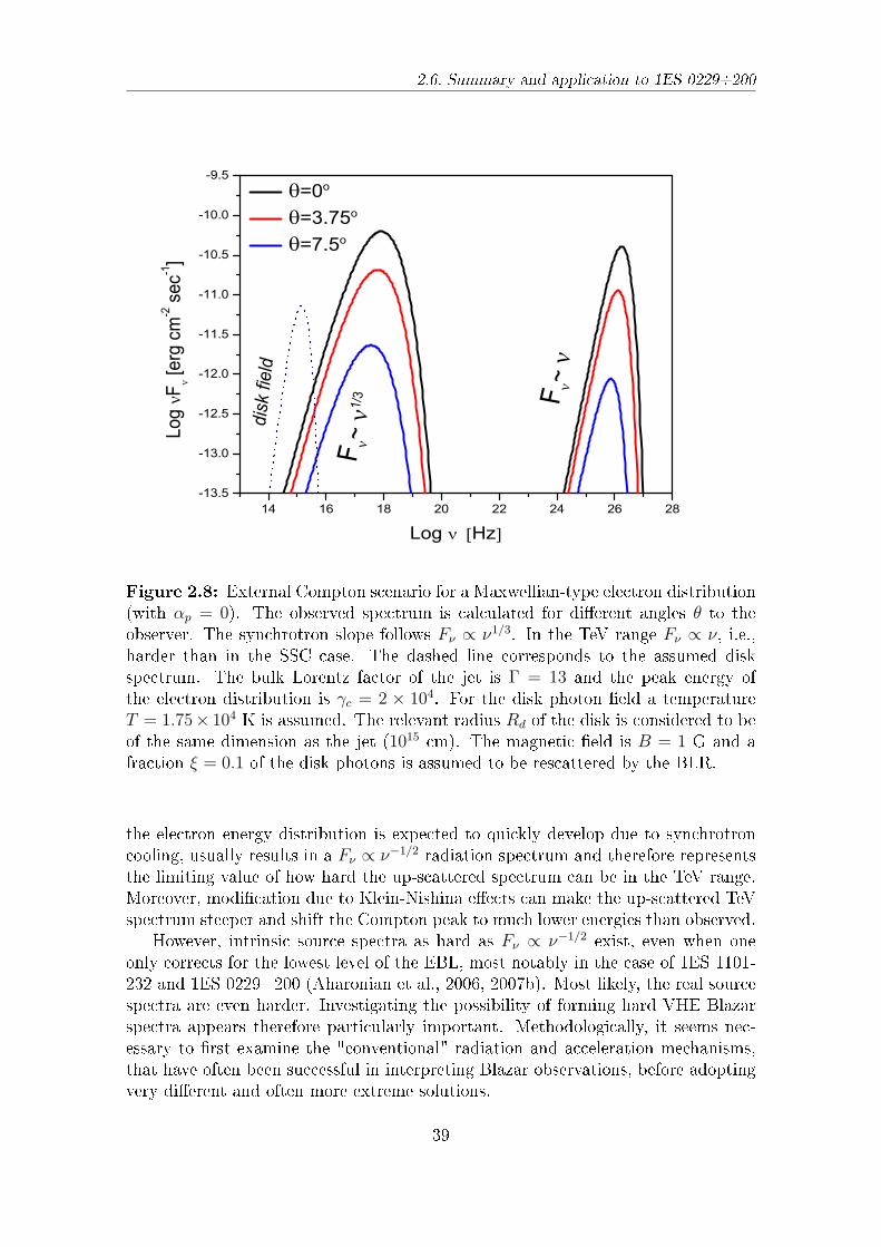
2.6. Summary and application to 1ES 0229+200
14 16 18 20 22 24 26 28-13.5
-13.0
-12.5
-12.0
-11.5
-11.0
-10.5
-10.0
-9.5
F~
F~
1/3
disk
fiel
d
Log
F [e
rg c
m-2 s
ec-1]
Log Hz
=0o
=3.75o
=7.5o
Figure 2.8: External Compton scenario for a Maxwellian-type electron distribution(with αp = 0). The observed spectrum is calculated for dierent angles θ to theobserver. The synchrotron slope follows Fν ∝ ν1/3. In the TeV range Fν ∝ ν, i.e.,harder than in the SSC case. The dashed line corresponds to the assumed diskspectrum. The bulk Lorentz factor of the jet is Γ = 13 and the peak energy ofthe electron distribution is γc = 2 × 10⁴. For the disk photon eld a temperatureT = 1.75× 10⁴ K is assumed. The relevant radius Rd of the disk is considered to beof the same dimension as the jet (1015 cm). The magnetic eld is B = 1 G and afraction ξ = 0.1 of the disk photons is assumed to be rescattered by the BLR.
the electron energy distribution is expected to quickly develop due to synchrotroncooling, usually results in a Fν ∝ ν−1/2 radiation spectrum and therefore representsthe limiting value of how hard the up-scattered spectrum can be in the TeV range.Moreover, modication due to Klein-Nishina eects can make the up-scattered TeVspectrum steeper and shift the Compton peak to much lower energies than observed.
However, intrinsic source spectra as hard as Fν ∝ ν−1/2 exist, even when oneonly corrects for the lowest level of the EBL, most notably in the case of 1ES 1101-232 and 1ES 0229+200 (Aharonian et al., 2006, 2007b). Most likely, the real sourcespectra are even harder. Investigating the possibility of forming hard VHE Blazarspectra appears therefore particularly important. Methodologically, it seems nec-essary to rst examine the "conventional" radiation and acceleration mechanisms,that have often been successful in interpreting Blazar observations, before adoptingvery dierent and often more extreme solutions.
39
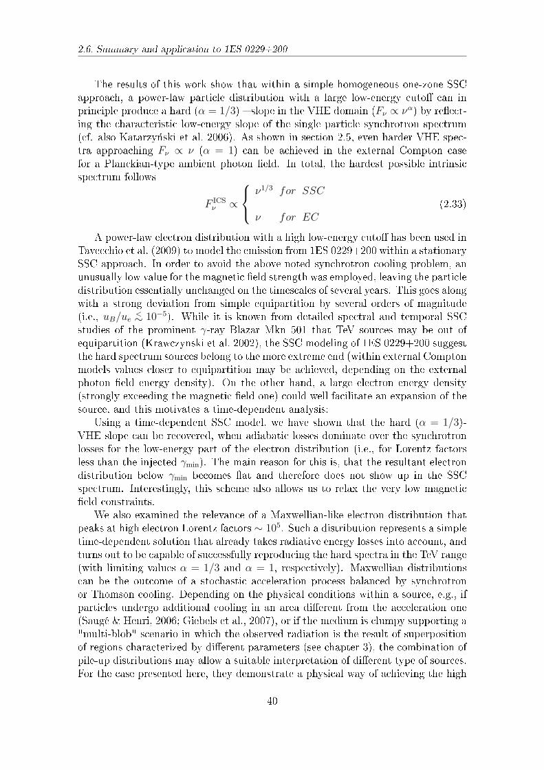
2.6. Summary and application to 1ES 0229+200
The results of this work show that within a simple homogeneous one-zone SSCapproach, a power-law particle distribution with a large low-energy cuto can inprinciple produce a hard (α = 1/3) slope in the VHE domain (Fν ∝ να) by reect-ing the characteristic low-energy slope of the single particle synchrotron spectrum(cf. also Katarzy«ski et al. 2006). As shown in section 2.5, even harder VHE spec-tra approaching Fν ∝ ν (α = 1) can be achieved in the external Compton casefor a Planckian-type ambient photon eld. In total, the hardest possible intrinsicspectrum follows
F ICSν ∝
ν1/3 for SSC
ν for EC(2.33)
A power-law electron distribution with a high low-energy cuto has been used inTavecchio et al. (2009) to model the emission from 1ES 0229+200 within a stationarySSC approach. In order to avoid the above noted synchrotron cooling problem, anunusually low value for the magnetic eld strength was employed, leaving the particledistribution essentially unchanged on the timescales of several years. This goes alongwith a strong deviation from simple equipartition by several orders of magnitude(i.e., uB/ue <∼ 10−5). While it is known from detailed spectral and temporal SSCstudies of the prominent γ-ray Blazar Mkn 501 that TeV sources may be out ofequipartition (Krawczynski et al. 2002), the SSC modeling of 1ES 0229+200 suggestthe hard spectrum sources belong to the more extreme end (within external Comptonmodels values closer to equipartition may be achieved, depending on the externalphoton eld energy density). On the other hand, a large electron energy density(strongly exceeding the magnetic eld one) could well facilitate an expansion of thesource, and this motivates a time-dependent analysis:
Using a time-dependent SSC model, we have shown that the hard (α = 1/3)-VHE slope can be recovered, when adiabatic losses dominate over the synchrotronlosses for the low-energy part of the electron distribution (i.e., for Lorentz factorsless than the injected γmin). The main reason for this is, that the resultant electrondistribution below γmin becomes at and therefore does not show up in the SSCspectrum. Interestingly, this scheme also allows us to relax the very low magneticeld constraints.
We also examined the relevance of a Maxwellian-like electron distribution thatpeaks at high electron Lorentz factors ∼ 105. Such a distribution represents a simpletime-dependent solution that already takes radiative energy losses into account, andturns out to be capable of successfully reproducing the hard spectra in the TeV range(with limiting values α = 1/3 and α = 1, respectively). Maxwellian distributionscan be the outcome of a stochastic acceleration process balanced by synchrotronor Thomson cooling. Depending on the physical conditions within a source, e.g., ifparticles undergo additional cooling in an area dierent from the acceleration one(Saugé & Henri, 2006; Giebels et al., 2007), or if the medium is clumpy supporting a"multi-blob" scenario in which the observed radiation is the result of superpositionof regions characterized by dierent parameters (see chapter 3), the combination ofpile-up distributions may allow a suitable interpretation of dierent type of sources.For the case presented here, they demonstrate a physical way of achieving the high
40
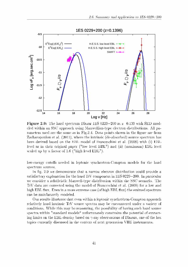
2.6. Summary and application to 1ES 0229+200
-12.5
-12
-11.5
-11
-10.5
-10
-9.5
14 16 18 20 22 24 26 28
Log
vFv
[erg
.sec
.cm
2 ]
Log v [Hz]
1ES 0229+200 (z=0.1396)
F v ∝
v1/
3
F v ∝
v1/
3
H.E.S.S. low level EBL
H.E.S.S. high level EBL
SWIFT
-12.5
-12
-11.5
-11
-10.5
-10
-9.5
14 16 18 20 22 24 26 28
Log
vFv
[erg
.sec
.cm
2 ]
Log v [Hz]
1ES 0229+200 (z=0.1396)
F v ∝
v1/
3
F v ∝
v1/
3
E2Exp[-(E/Ec)3]
E2Exp[-E/Ec]
Figure 2.9: The hard spectrum Blazar 1ES 0229+200 at z=0.139 with SED mod-eled within an SSC approach using Maxwellian-type electron distributions. All pa-rameters used are the same as in Fig.2.4. Data points shown in the gure are fromZacharopoulou et al. (2011), where the intrinsic (de-absorbed) source spectrum hasbeen derived based on the EBL model of Franceschini et al. (2008) with (i) EBLlevel as in their original paper ("low level EBL") and (ii) (maximum) EBL levelscaled up by a factor of 1.6 ("high level EBL").
low-energy cutos needed in leptonic synchrotron-Compton models for the hardspectrum sources.
In g. 2.9 we demonstrate that a narrow electron distribution could provide asatisfactory explanation for the hard TeV component in 1ES 0229+200. In particularwe consider a relativistic Maxwell-type distribution within the SSC scenario. TheTeV data are corrected using the model of Franceschini et al. (2008) for a low andhigh EBL ux. Even in a more extreme case (of high EBL ux) the emitted spectrumcan be satisfactorily modeled.
Our results illustrate that even within a leptonic synchrotron-Compton approachrelatively hard intrinsic TeV source spectra may be encountered under a variety ofconditions. While this may be reassuring, the possibility of having such hard sourcespectra within "standard models" unfortunately constrains the potential of extract-ing limits on the EBL density based on γ-ray observations of Blazars, one of the hottopics currently discussed in the context of next generation VHE instruments.
41

2.6. Summary and application to 1ES 0229+200
42
Chapter 3
"Leading blob" model in a stochastic
acceleration scenario
Evidence for very hard, intrinsic γ-ray source spectra, as inferred after correc-tion for the absorption in the extragalactic background light (EBL), has interestingimplications for the acceleration and radiation mechanisms acting in Blazars. A keyissue so far has been the dependance of the hardness of the γ-ray spectrum on dier-ent existing EBL models. The recent FERMI observations of Mkn 501 now provideadditional evidence for the presence of hard intrinsic γ-ray spectra independent ofEBL uncertainties. Relativistic Maxwellian-type electron energy distributions thatare formed in stochastic acceleration scenarios oer a plausible interpretation forsuch hard source spectra. In this chapter we show that the combined emission fromdierent components with Maxwellian-type distributions could in principle also ac-count for much softer and broader, power law-like emission spectra. We introducea "leading blob" scenario, applicable to active aring episodes, when one (or a few)of these components become distinct over the "background" emission, producinghard spectral features and/or hardening of the observed spectra. We show thatthis model can explain the peculiar high-energy characteristics of Mkn 501 in 2009,with evidence for aring activity and strong spectral hardening at the highest γ-rayenergies1.
3.1 The 2009 hard are of Mkn 501
In the previous chapter we discussed in detail the problems arising in the inter-pretation of hard spectra within standard leptonic scenarios, i.e., SSC or EC models.The noted small photon indices are generally not easy to achieve, because radiativecooling tends to produce particle energy distributions that are always steeper thandNγ/dEγ ∝ E−2
γ , irrespective of the initially injected particle spectrum. The corre-sponding TeV photon index would then be Γ ≥ 1.5. Moreover, as the emission fromthese objects peaks at very high energies, where suppression of the cross-section dueto Klein-Nishina eects becomes important, even steeper intrinsic photon spectra
1The results discussed in this chapter are based on Lefa et al. 2011b
43
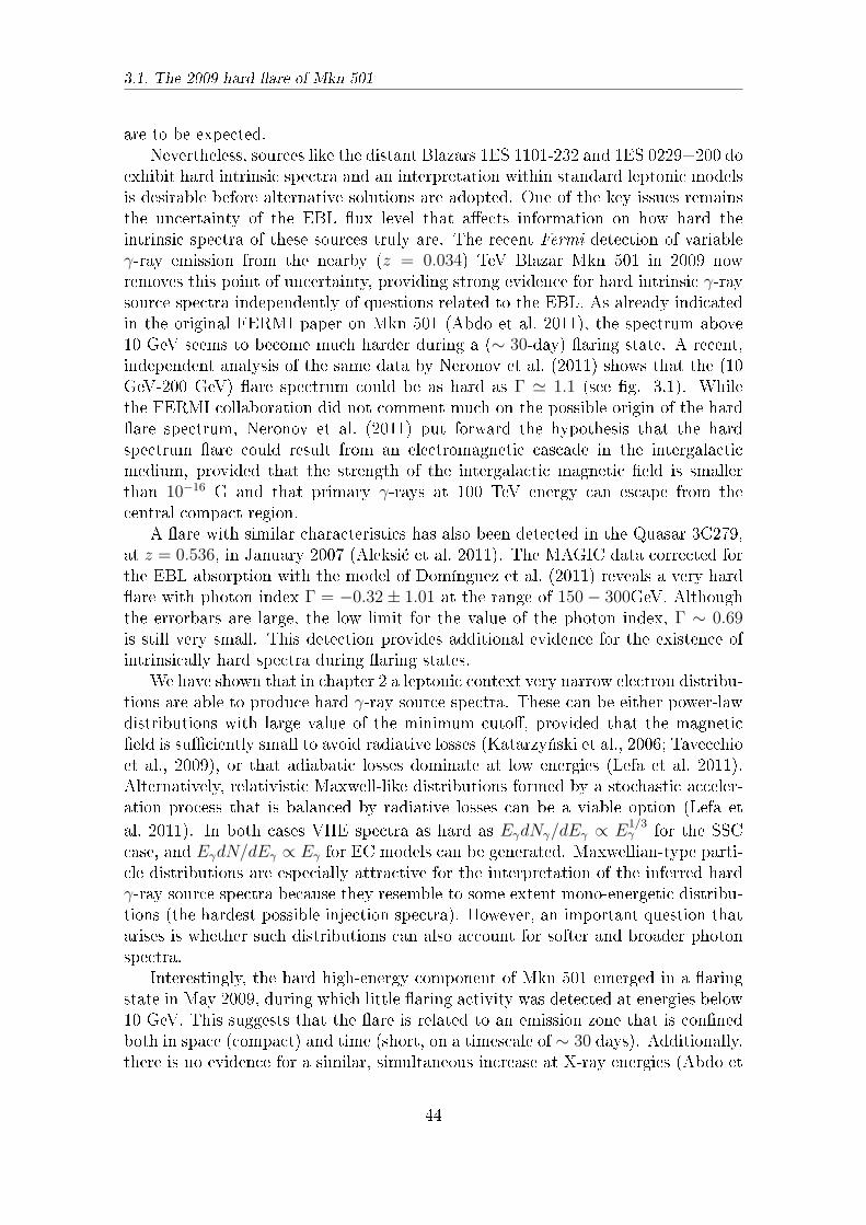
3.1. The 2009 hard are of Mkn 501
are to be expected.Nevertheless, sources like the distant Blazars 1ES 1101-232 and 1ES 0229+200 do
exhibit hard intrinsic spectra and an interpretation within standard leptonic modelsis desirable before alternative solutions are adopted. One of the key issues remainsthe uncertainty of the EBL ux level that aects information on how hard theintrinsic spectra of these sources truly are. The recent Fermi detection of variableγ-ray emission from the nearby (z = 0.034) TeV Blazar Mkn 501 in 2009 nowremoves this point of uncertainty, providing strong evidence for hard intrinsic γ-raysource spectra independently of questions related to the EBL. As already indicatedin the original FERMI paper on Mkn 501 (Abdo et al. 2011), the spectrum above10 GeV seems to become much harder during a (∼ 30-day) aring state. A recent,independent analysis of the same data by Neronov et al. (2011) shows that the (10GeV-200 GeV) are spectrum could be as hard as Γ ≃ 1.1 (see g. 3.1). Whilethe FERMI collaboration did not comment much on the possible origin of the hardare spectrum, Neronov et al. (2011) put forward the hypothesis that the hardspectrum are could result from an electromagnetic cascade in the intergalacticmedium, provided that the strength of the intergalactic magnetic eld is smallerthan 10−16 G and that primary γ-rays at 100 TeV energy can escape from thecentral compact region.
A are with similar characteristics has also been detected in the Quasar 3C279,at z = 0.536, in January 2007 (Aleksi¢ et al. 2011). The MAGIC data corrected forthe EBL absorption with the model of Domínguez et al. (2011) reveals a very hardare with photon index Γ = −0.32± 1.01 at the range of 150− 300GeV. Althoughthe errorbars are large, the low limit for the value of the photon index, Γ ∼ 0.69is still very small. This detection provides additional evidence for the existence ofintrinsically hard spectra during aring states.
We have shown that in chapter 2 a leptonic context very narrow electron distribu-tions are able to produce hard γ-ray source spectra. These can be either power-lawdistributions with large value of the minimum cuto, provided that the magneticeld is suciently small to avoid radiative losses (Katarzy«ski et al., 2006; Tavecchioet al., 2009), or that adiabatic losses dominate at low energies (Lefa et al. 2011).Alternatively, relativistic Maxwell-like distributions formed by a stochastic acceler-ation process that is balanced by radiative losses can be a viable option (Lefa etal. 2011). In both cases VHE spectra as hard as EγdNγ/dEγ ∝ E
1/3γ for the SSC
case, and EγdN/dEγ ∝ Eγ for EC models can be generated. Maxwellian-type parti-cle distributions are especially attractive for the interpretation of the inferred hardγ-ray source spectra because they resemble to some extent mono-energetic distribu-tions (the hardest possible injection spectra). However, an important question thatarises is whether such distributions can also account for softer and broader photonspectra.
Interestingly, the hard high-energy component of Mkn 501 emerged in a aringstate in May 2009, during which little aring activity was detected at energies below10 GeV. This suggests that the are is related to an emission zone that is connedboth in space (compact) and time (short, on a timescale of ∼ 30 days). Additionally,there is no evidence for a similar, simultaneous increase at X-ray energies (Abdo et
44
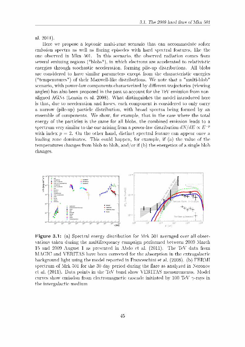
3.1. The 2009 hard are of Mkn 501
al. 2011).Here we propose a leptonic multi-zone scenario that can accommodate softer
emission spectra as well as aring episodes with hard spectral features, like theone observed in Mkn 501. In this scenario, the observed radiation comes fromseveral emitting regions ("blobs"), in which electrons are accelerated to relativisticenergies through stochastic acceleration, forming pile-up distributions. All blobsare considered to have similar parameters except from the characteristic energies("temperatures") of their Maxwell-like distributions. We note that a "multi-blob"scenario, with power-law components characterized by dierent trajectories (viewingangles) has also been proposed in the past to account for the TeV emission from non-aligned AGNs (Lenain et al. 2008). What distinguishes the model introduced hereis that, due to acceleration and losses, each component is considered to only carrya narrow (pile-up) particle distribution, with broad spectra being formed by anensemble of components. We show, for example, that in the case where the totalenergy of the particles is the same for all blobs, the combined emission leads to aspectrum very similar to the one arising from a power-law distribution dN/dE ∝ E−p
with index p = 2. On the other hand, distinct spectral feature can appear once aleading zone dominates. This could happen, for example, if (a) the value of thetemperatures changes from blob to blob, and/or if (b) the energetics of a single blobchanges.
[Hz]ν1010 1210 1410 1610 1810 2010 2210 2410 2610 2810
]-1
s-2
[erg
cm
ν Fν
-1410
-1310
-1210
-1110
-1010
-910
MAGIC
VERITAS
VERITAS_flare
Fermi
Swift/BAT
RXTE/PCA
Swift/XRT
Swift/UVOT
BradfordRoboticTelescope
GASP
GRT
MITSuME
ROVOR
WIRO
OAGH
CampoImperatore
SMA
VLBA(BP143)
VLBA_core(BP143)
VLBA_core_ellipsefit(BP143)
VLBA(BK150)
VLBA_core(BK150)
Noto
Metsahovi
Medicina
VLBA(MOJAVE)
VLBA_Core(MOJAVE)
OVRO
RATAN
UMRAO
Effelsberg
Figure 3.1: (a) Spectral energy distribution for Mrk 501 averaged over all obser-vations taken during the multifrequency campaign performed between 2009 March15 and 2009 August 1 as presented in Abdo et al. (2011). The TeV data fromMAGIC and VERITAS have been corrected for the absorption in the extragalacticbackground light using the model reported in Franceschini et al. (2008). (b) FERMIspectrum of Mrk 501 for the 30 day period during the are as analyzed in Neronovet al. (2011). Data points in the TeV band show VERITAS measurements. Modelcurves show emission from electromagnetic cascade initiated by 100 TeV γ-rays inthe intergalactic medium
45
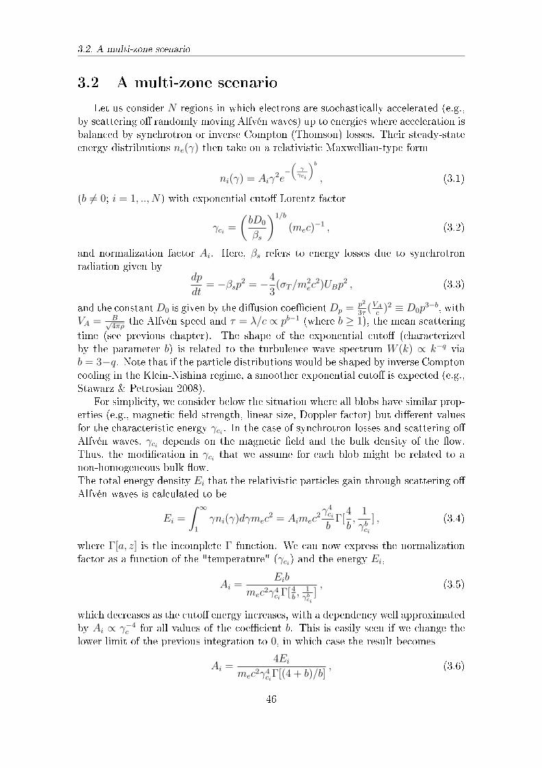
3.2. A multi-zone scenario
3.2 A multi-zone scenario
Let us consider N regions in which electrons are stochastically accelerated (e.g.,by scattering o randomly moving Alfvén waves) up to energies where acceleration isbalanced by synchrotron or inverse Compton (Thomson) losses. Their steady-stateenergy distributions ne(γ) then take on a relativistic Maxwellian-type form
ni(γ) = Aiγ2e
−(
γγci
)b
, (3.1)
(b = 0; i = 1, .., N) with exponential cuto Lorentz factor
γci =
(bD0
βs
)1/b
(mec)−1 , (3.2)
and normalization factor Ai. Here, βs refers to energy losses due to synchrotronradiation given by
dp
dt= −βsp
2 = −4
3(σT/m
2ec
2)UBp2 , (3.3)
and the constantD0 is given by the diusion coecientDp =p2
3τ(VAc)2 ≡ D0p
3−b, withVA = B√
4πρthe Alfvén speed and τ = λ/c ∝ pb−1 (where b ≥ 1), the mean scattering
time (see previous chapter). The shape of the exponential cuto (characterizedby the parameter b) is related to the turbulence wave spectrum W (k) ∝ k−q viab = 3−q. Note that if the particle distributions would be shaped by inverse Comptoncooling in the Klein-Nishina regime, a smoother exponential cuto is expected (e.g.,Stawarz & Petrosian 2008).
For simplicity, we consider below the situation where all blobs have similar prop-erties (e.g., magnetic eld strength, linear size, Doppler factor) but dierent valuesfor the characteristic energy γci . In the case of synchrotron losses and scattering oAlfvén waves, γci depends on the magnetic eld and the bulk density of the ow.Thus, the modication in γci that we assume for each blob might be related to anon-homogeneous bulk ow.The total energy density Ei that the relativistic particles gain through scattering oAlfvén waves is calculated to be
Ei =
∫ ∞
1
γni(γ)dγmec2 = Aimec
2γ4ci
bΓ[4
b,1
γbci] , (3.4)
where Γ[a, z] is the incomplete Γ function. We can now express the normalizationfactor as a function of the "temperature" (γci) and the energy Ei,
Ai =Eib
mec2γ4ciΓ[4
b, 1γbci
], (3.5)
which decreases as the cuto energy increases, with a dependency well approximatedby Ai ∝ γ−4
c for all values of the coecient b. This is easily seen if we change thelower limit of the previous integration to 0, in which case the result becomes
Ai =4Ei
mec2γ4ciΓ[(4 + b)/b]
, (3.6)
46
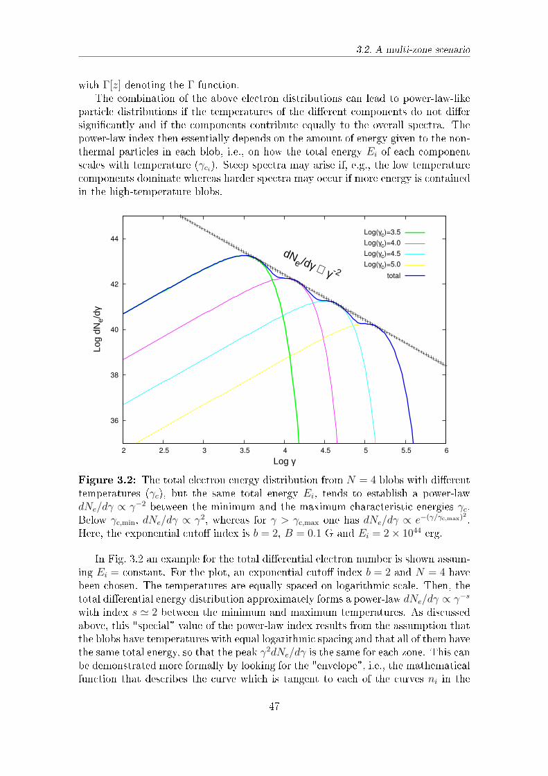
3.2. A multi-zone scenario
with Γ[z] denoting the Γ function.The combination of the above electron distributions can lead to power-law-like
particle distributions if the temperatures of the dierent components do not diersignicantly and if the components contribute equally to the overall spectra. Thepower-law index then essentially depends on the amount of energy given to the non-thermal particles in each blob, i.e., on how the total energy Ei of each componentscales with temperature (γci). Steep spectra may arise if, e.g., the low temperaturecomponents dominate whereas harder spectra may occur if more energy is containedin the high-temperature blobs.
36
38
40
42
44
2 2.5 3 3.5 4 4.5 5 5.5 6
Log
dNe/
dγ
Log γ
dNe /dγ ∝ γ -2
Log(γc)=3.5
Log(γc)=4.0
Log(γc)=4.5
Log(γc)=5.0
total
Figure 3.2: The total electron energy distribution from N = 4 blobs with dierenttemperatures (γc), but the same total energy Ei, tends to establish a power-lawdNe/dγ ∝ γ−2 between the minimum and the maximum characteristic energies γc.Below γc,min, dNe/dγ ∝ γ2, whereas for γ > γc,max one has dNe/dγ ∝ e−(γ/γc,max)2 .Here, the exponential cuto index is b = 2, B = 0.1 G and Ei = 2× 1044 erg.
In Fig. 3.2 an example for the total dierential electron number is shown assum-ing Ei = constant. For the plot, an exponential cuto index b = 2 and N = 4 havebeen chosen. The temperatures are equally spaced on logarithmic scale. Then, thetotal dierential energy distribution approximately forms a power-law dNe/dγ ∝ γ−s
with index s ≃ 2 between the minimum and maximum temperatures. As discussedabove, this "special" value of the power-law index results from the assumption thatthe blobs have temperatures with equal logarithmic spacing and that all of them havethe same total energy, so that the peak γ2dNe/dγ is the same for each zone. This canbe demonstrated more formally by looking for the "envelope", i.e., the mathematicalfunction that describes the curve which is tangent to each of the curves ni in the
47
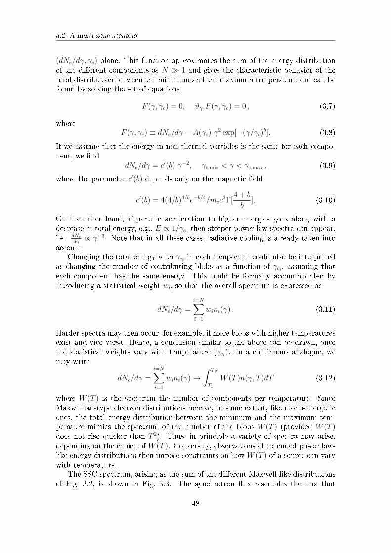
3.2. A multi-zone scenario
(dNe/dγ, γc) plane. This function approximates the sum of the energy distributionof the dierent components as N ≫ 1 and gives the characteristic behavior of thetotal distribution between the minimum and the maximum temperature and can befound by solving the set of equations
F (γ, γc) = 0, ϑγcF (γ, γc) = 0 , (3.7)
whereF (γ, γc) ≡ dNe/dγ − A(γc) γ
2 exp[−(γ/γc)b]. (3.8)
If we assume that the energy in non-thermal particles is the same for each compo-nent, we nd
dNe/dγ = c′(b) γ−2, γc,min < γ < γc,max , (3.9)
where the parameter c′(b) depends only on the magnetic eld
c′(b) = 4(4/b)4/be−b/4/mec2Γ[
4 + b
b]. (3.10)
On the other hand, if particle acceleration to higher energies goes along with adecrease in total energy, e.g., E ∝ 1/γc, then steeper power law spectra can appear,i.e., dNe
dγ∝ γ−3. Note that in all these cases, radiative cooling is already taken into
account.Changing the total energy with γci in each component could also be interpreted
as changing the number of contributing blobs as a function of γci , assuming thateach component has the same energy. This could be formally accommodated byintroducing a statistical weight wi, so that the overall spectrum is expressed as
dNe/dγ =i=N∑i=1
wini(γ) . (3.11)
Harder spectra may then occur, for example, if more blobs with higher temperaturesexist and vice versa. Hence, a conclusion similar to the above can be drawn, oncethe statistical weights vary with temperature (γci). In a continuous analogue, wemay write
dNe/dγ =i=N∑i=1
wini(γ) →∫ TN
T1
W (T )n(γ, T )dT (3.12)
where W (T ) is the spectrum the number of components per temperature. SinceMaxwellian-type electron distributions behave, to some extent, like mono-energeticones, the total energy distribution between the minimum and the maximum tem-perature mimics the spectrum of the number of the blobs W (T ) (provided W (T )does not rise quicker than T 2). Thus, in principle a variety of spectra may arise,depending on the choice of W (T ). Conversely, observations of extended power law-like energy distributions then impose constraints on how W (T ) of a source can varywith temperature.
The SSC spectrum, arising as the sum of the dierent Maxwell-like distributionsof Fig. 3.2, is shown in Fig. 3.3. The synchrotron ux resembles the ux that
48
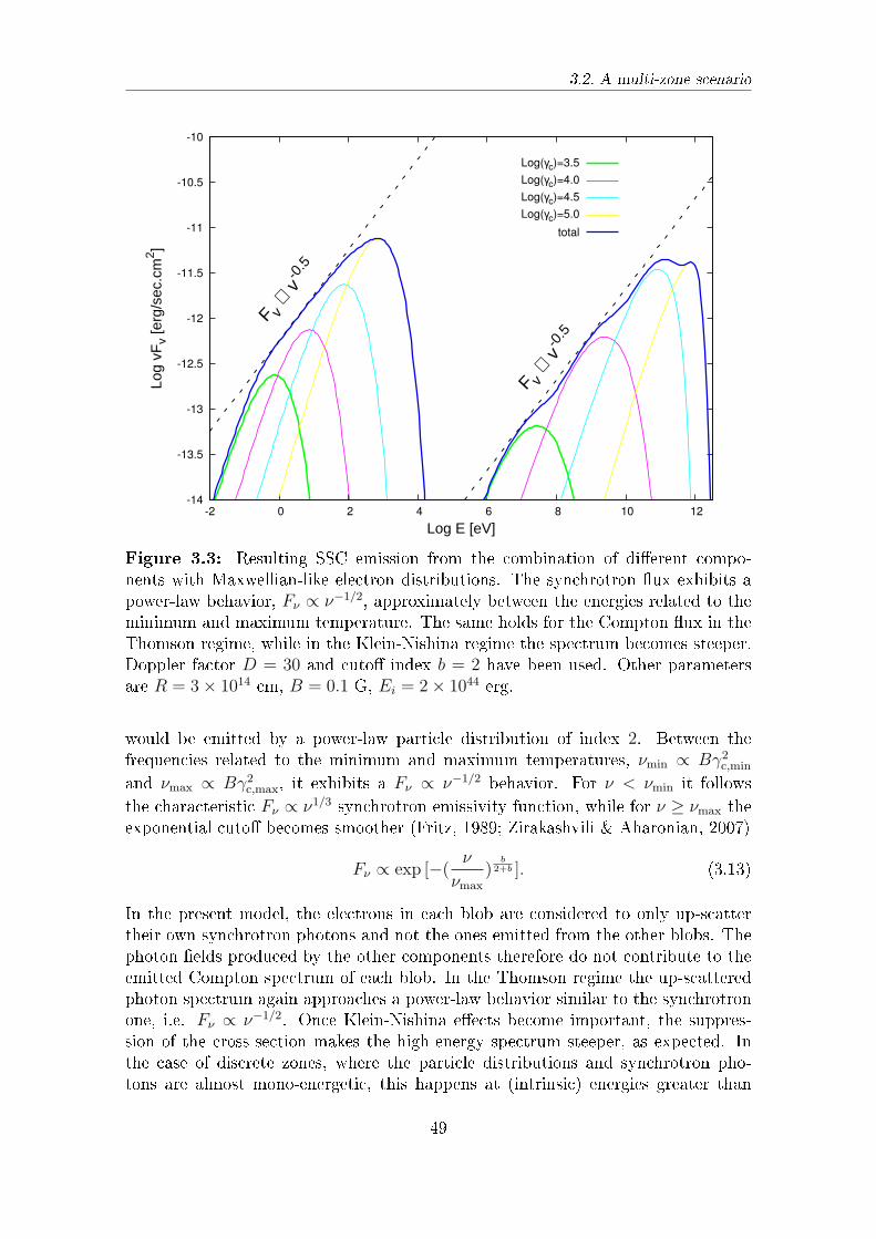
3.2. A multi-zone scenario
-14
-13.5
-13
-12.5
-12
-11.5
-11
-10.5
-10
-2 0 2 4 6 8 10 12
Log
vFv
[erg
/sec
.cm
2 ]
Log E [eV]F v
∝ v
-0.5
F v ∝
v-0
.5
Log(γc)=3.5
Log(γc)=4.0
Log(γc)=4.5
Log(γc)=5.0
total
Figure 3.3: Resulting SSC emission from the combination of dierent compo-nents with Maxwellian-like electron distributions. The synchrotron ux exhibits apower-law behavior, Fν ∝ ν−1/2, approximately between the energies related to theminimum and maximum temperature. The same holds for the Compton ux in theThomson regime, while in the Klein-Nishina regime the spectrum becomes steeper.Doppler factor D = 30 and cuto index b = 2 have been used. Other parametersare R = 3× 1014 cm, B = 0.1 G, Ei = 2× 1044 erg.
would be emitted by a power-law particle distribution of index 2. Between thefrequencies related to the minimum and maximum temperatures, νmin ∝ Bγ2
c,min
and νmax ∝ Bγ2c,max, it exhibits a Fν ∝ ν−1/2 behavior. For ν < νmin it follows
the characteristic Fν ∝ ν1/3 synchrotron emissivity function, while for ν ≥ νmax theexponential cuto becomes smoother (Fritz, 1989; Zirakashvili & Aharonian, 2007)
Fν ∝ exp [−(ν
νmax
)b
2+b ]. (3.13)
In the present model, the electrons in each blob are considered to only up-scattertheir own synchrotron photons and not the ones emitted from the other blobs. Thephoton elds produced by the other components therefore do not contribute to theemitted Compton spectrum of each blob. In the Thomson regime the up-scatteredphoton spectrum again approaches a power-law behavior similar to the synchrotronone, i.e. Fν ∝ ν−1/2. Once Klein-Nishina eects become important, the suppres-sion of the cross-section makes the high-energy spectrum steeper, as expected. Inthe case of discrete zones, where the particle distributions and synchrotron pho-tons are almost mono-energetic, this happens at (intrinsic) energies greater than
49
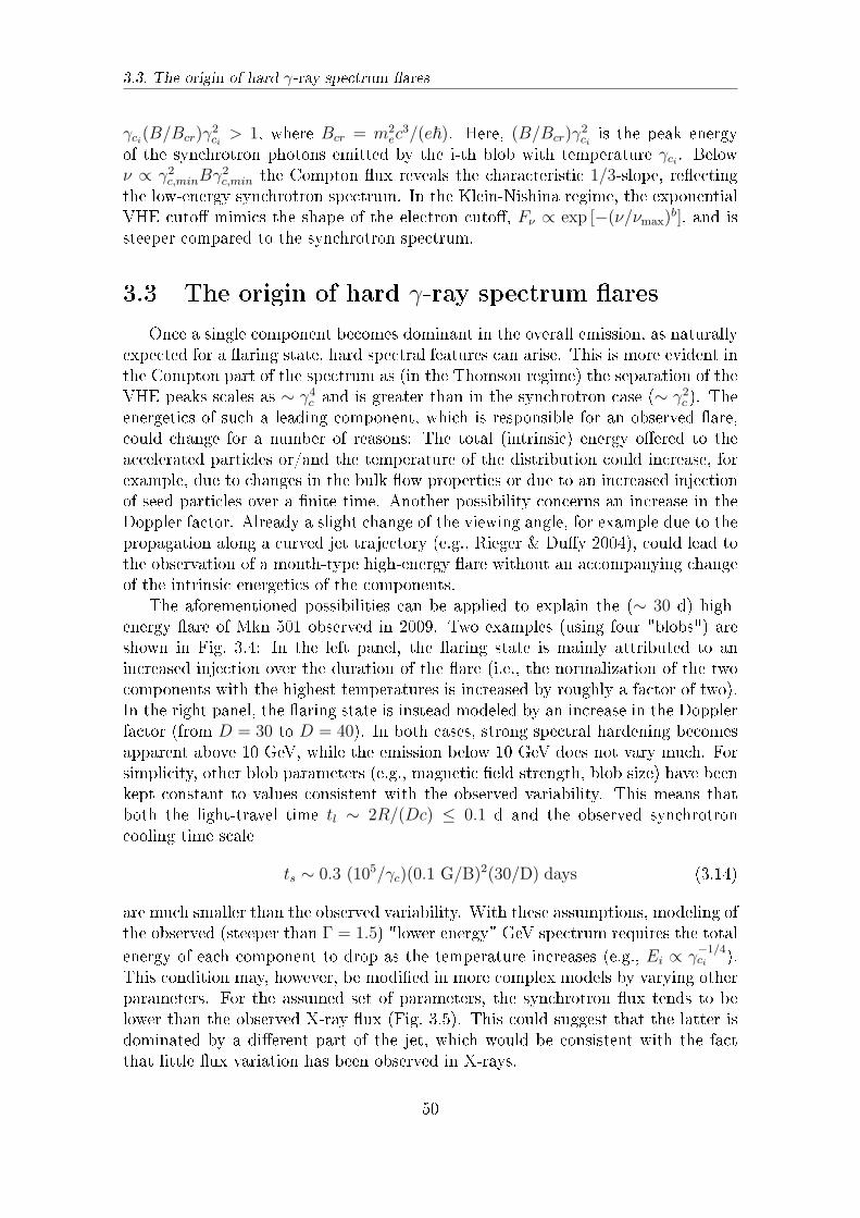
3.3. The origin of hard γ-ray spectrum ares
γci(B/Bcr)γ2ci
> 1, where Bcr = m2ec
3/(e~). Here, (B/Bcr)γ2ciis the peak energy
of the synchrotron photons emitted by the i-th blob with temperature γci . Belowν ∝ γ2
c,minBγ2c,min the Compton ux reveals the characteristic 1/3-slope, reecting
the low-energy synchrotron spectrum. In the Klein-Nishina regime, the exponentialVHE cuto mimics the shape of the electron cuto, Fν ∝ exp [−(ν/νmax)
b], and issteeper compared to the synchrotron spectrum.
3.3 The origin of hard γ-ray spectrum ares
Once a single component becomes dominant in the overall emission, as naturallyexpected for a aring state, hard spectral features can arise. This is more evident inthe Compton part of the spectrum as (in the Thomson regime) the separation of theVHE peaks scales as ∼ γ4
c and is greater than in the synchrotron case (∼ γ2c ). The
energetics of such a leading component, which is responsible for an observed are,could change for a number of reasons: The total (intrinsic) energy oered to theaccelerated particles or/and the temperature of the distribution could increase, forexample, due to changes in the bulk ow properties or due to an increased injectionof seed particles over a nite time. Another possibility concerns an increase in theDoppler factor. Already a slight change of the viewing angle, for example due to thepropagation along a curved jet trajectory (e.g., Rieger & Duy 2004), could lead tothe observation of a month-type high-energy are without an accompanying changeof the intrinsic energetics of the components.
The aforementioned possibilities can be applied to explain the (∼ 30 d) high-energy are of Mkn 501 observed in 2009. Two examples (using four "blobs") areshown in Fig. 3.4: In the left panel, the aring state is mainly attributed to anincreased injection over the duration of the are (i.e., the normalization of the twocomponents with the highest temperatures is increased by roughly a factor of two).In the right panel, the aring state is instead modeled by an increase in the Dopplerfactor (from D = 30 to D = 40). In both cases, strong spectral hardening becomesapparent above 10 GeV, while the emission below 10 GeV does not vary much. Forsimplicity, other blob parameters (e.g., magnetic eld strength, blob size) have beenkept constant to values consistent with the observed variability. This means thatboth the light-travel time tl ∼ 2R/(Dc) ≤ 0.1 d and the observed synchrotroncooling time scale
ts ∼ 0.3 (105/γc)(0.1 G/B)2(30/D) days (3.14)
are much smaller than the observed variability. With these assumptions, modeling ofthe observed (steeper than Γ = 1.5) "lower energy" GeV spectrum requires the totalenergy of each component to drop as the temperature increases (e.g., Ei ∝ γ
−1/4ci ).
This condition may, however, be modied in more complex models by varying otherparameters. For the assumed set of parameters, the synchrotron ux tends to belower than the observed X-ray ux (Fig. 3.5). This could suggest that the latter isdominated by a dierent part of the jet, which would be consistent with the factthat little ux variation has been observed in X-rays.
50
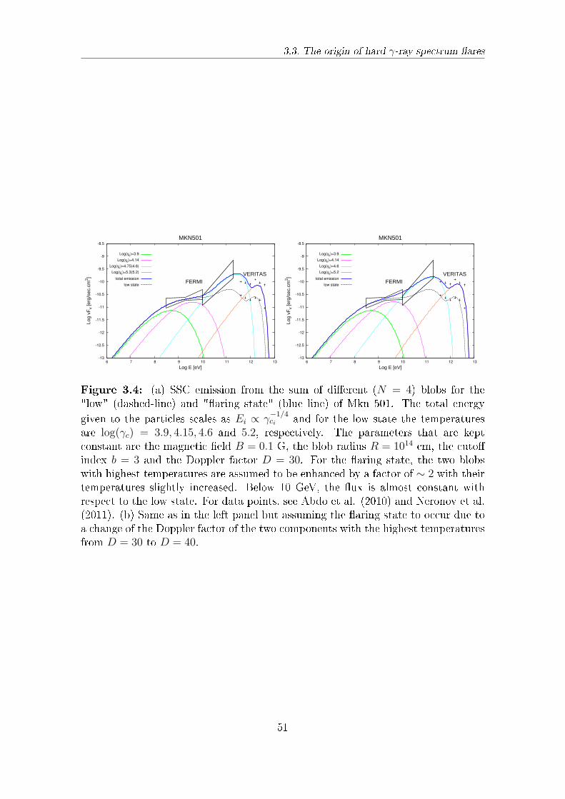
3.3. The origin of hard γ-ray spectrum ares
-13
-12.5
-12
-11.5
-11
-10.5
-10
-9.5
-9
-8.5
6 7 8 9 10 11 12 13
Log
vFv
[erg
/sec
.cm
2 ]
Log E [eV]
MKN501
FERMIVERITAS
Log(γc)=3.9
Log(γc)=4.14
Log(γc)=4.75(4.6)
Log(γc)=5.3(5.2)
total emission
low state
-13
-12.5
-12
-11.5
-11
-10.5
-10
-9.5
-9
-8.5
6 7 8 9 10 11 12 13
Log
vFv
[erg
/sec
.cm
2 ]
Log E [eV]
MKN501
FERMIVERITAS
Log(γc)=3.9
Log(γc)=4.14
Log(γc)=4.6
Log(γc)=5.2
total emission
low state
Figure 3.4: (a) SSC emission from the sum of dierent (N = 4) blobs for the"low" (dashed-line) and "aring state" (blue line) of Mkn 501. The total energygiven to the particles scales as Ei ∝ γ
−1/4ci and for the low state the temperatures
are log(γc) = 3.9, 4.15, 4.6 and 5.2, respectively. The parameters that are keptconstant are the magnetic eld B = 0.1 G, the blob radius R = 1014 cm, the cutoindex b = 3 and the Doppler factor D = 30. For the aring state, the two blobswith highest temperatures are assumed to be enhanced by a factor of ∼ 2 with theirtemperatures slightly increased. Below 10 GeV, the ux is almost constant withrespect to the low state. For data points, see Abdo et al. (2010) and Neronov et al.(2011). (b) Same as in the left panel but assuming the aring state to occur due toa change of the Doppler factor of the two components with the highest temperaturesfrom D = 30 to D = 40.
51
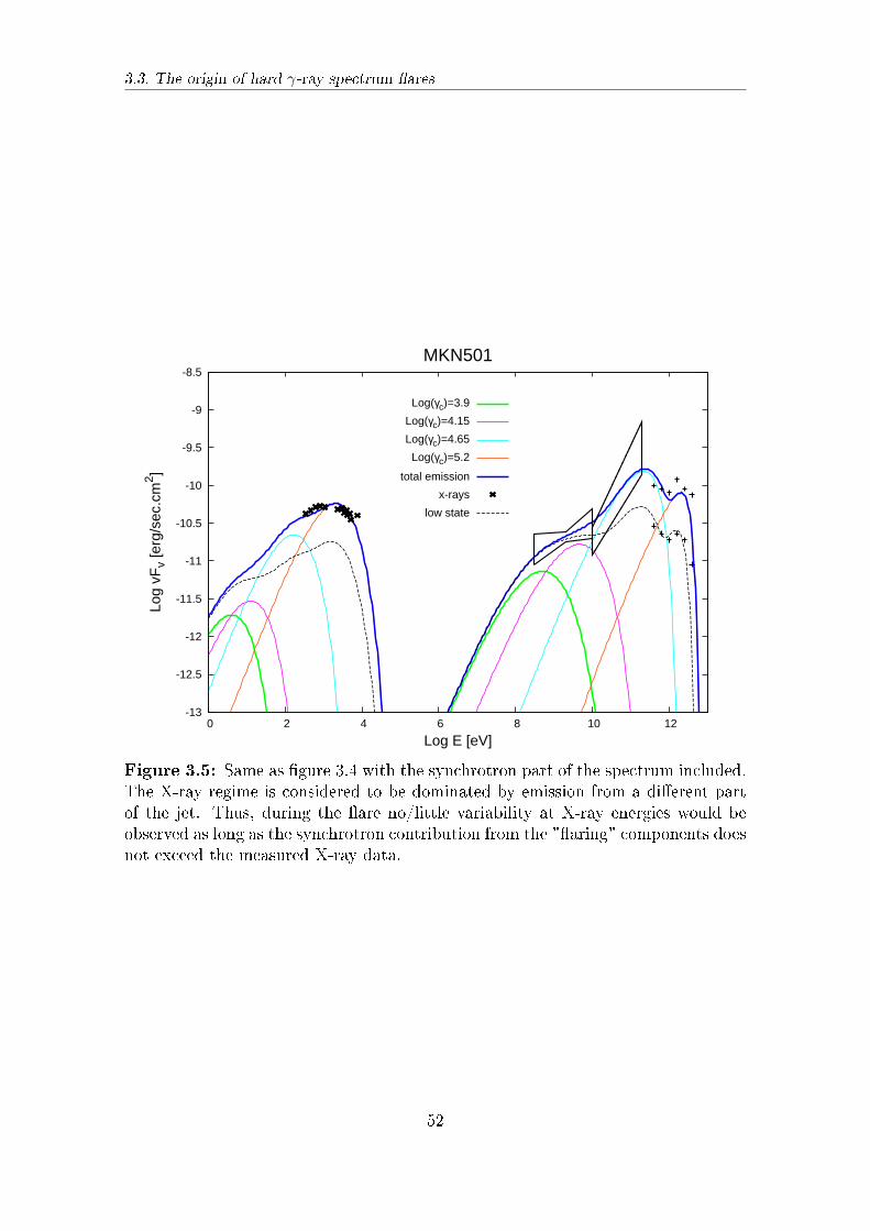
3.3. The origin of hard γ-ray spectrum ares
-13
-12.5
-12
-11.5
-11
-10.5
-10
-9.5
-9
-8.5
0 2 4 6 8 10 12
Log
vFv
[erg
/sec
.cm
2 ]
Log E [eV]
MKN501
Log(γc)=3.9
Log(γc)=4.15
Log(γc)=4.65
Log(γc)=5.2
total emission
x-rays
low state
Figure 3.5: Same as gure 3.4 with the synchrotron part of the spectrum included.The X-ray regime is considered to be dominated by emission from a dierent partof the jet. Thus, during the are no/little variability at X-ray energies would beobserved as long as the synchrotron contribution from the "aring" components doesnot exceed the measured X-ray data.
52
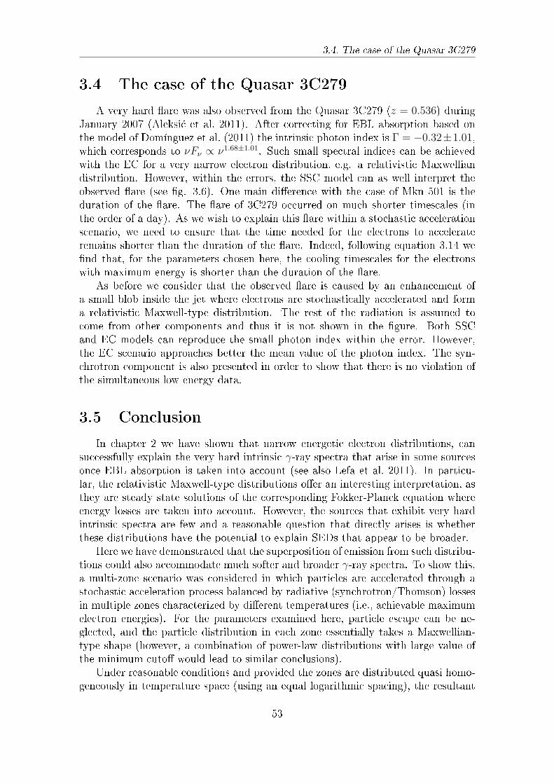
3.4. The case of the Quasar 3C279
3.4 The case of the Quasar 3C279
A very hard are was also observed from the Quasar 3C279 (z = 0.536) duringJanuary 2007 (Aleksi¢ et al. 2011). After correcting for EBL absorption based onthe model of Domínguez et al. (2011) the intrinsic photon index is Γ = −0.32±1.01,which corresponds to νFν ∝ ν1.68±1.01. Such small spectral indices can be achievedwith the EC for a very narrow electron distribution, e.g. a relativistic Maxwelliandistribution. However, within the errors, the SSC model can as well interpret theobserved are (see g. 3.6). One main dierence with the case of Mkn 501 is theduration of the are. The are of 3C279 occurred on much shorter timescales (inthe order of a day). As we wish to explain this are within a stochastic accelerationscenario, we need to ensure that the time needed for the electrons to accelerateremains shorter than the duration of the are. Indeed, following equation 3.14 wend that, for the parameters chosen here, the cooling timescales for the electronswith maximum energy is shorter than the duration of the are.
As before we consider that the observed are is caused by an enhancement ofa small blob inside the jet where electrons are stochastically accelerated and forma relativistic Maxwell-type distribution. The rest of the radiation is assumed tocome from other components and thus it is not shown in the gure. Both SSCand EC models can reproduce the small photon index within the error. However,the EC scenario approaches better the mean value of the photon index. The syn-chrotron component is also presented in order to show that there is no violation ofthe simultaneous low energy data.
3.5 Conclusion
In chapter 2 we have shown that narrow energetic electron distributions, cansuccessfully explain the very hard intrinsic γ-ray spectra that arise in some sourcesonce EBL absorption is taken into account (see also Lefa et al. 2011). In particu-lar, the relativistic Maxwell-type distributions oer an interesting interpretation, asthey are steady state solutions of the corresponding Fokker-Planck equation whereenergy losses are taken into account. However, the sources that exhibit very hardintrinsic spectra are few and a reasonable question that directly arises is whetherthese distributions have the potential to explain SEDs that appear to be broader.
Here we have demonstrated that the superposition of emission from such distribu-tions could also accommodate much softer and broader γ-ray spectra. To show this,a multi-zone scenario was considered in which particles are accelerated through astochastic acceleration process balanced by radiative (synchrotron/Thomson) lossesin multiple zones characterized by dierent temperatures (i.e., achievable maximumelectron energies). For the parameters examined here, particle escape can be ne-glected, and the particle distribution in each zone essentially takes a Maxwellian-type shape (however, a combination of power-law distributions with large value ofthe minimum cuto would lead to similar conclusions).
Under reasonable conditions and provided the zones are distributed quasi homo-geneously in temperature space (using an equal logarithmic spacing), the resultant
53
3.5. Conclusion
-13
-12.5
-12
-11.5
-11
-10.5
-10
-9.5
-9
10 12 14 16 18 20 22 24 26 28
Log
(vF
v) [e
rg/c
m2 se
c]
Log v [Hz]
SSC fromMaxwell-like electrons
optical
x-rays
Magic deabsorbed
Magic observed
-13
-12.5
-12
-11.5
-11
-10.5
-10
-9.5
-9
12 14 16 18 20 22 24 26
Log
(vF
v) [e
rg/c
m2 se
c]
Log v [Hz]
EC fromMaxwell-like electrons
optical
x-rays
Magic deabsorbed
Magic observed
"softphotons.dat"
Figure 3.6: (a) SSC emission from Maxwellian electrons for the Quasar 3C279. Theparameters used are the electron cuto energy γc = 7 × 10⁴, the index β = 2, themagnetic eld B = 0.3G, the source radius R = 1014cm and the Doppler factor δ =40. The deviation from equipartition is Log (Ue/UB) = 4.8. The (theoretical) slopeat the high energy data is somewhat less than 4/3, from 0.8 to 1 approximately. Allthe data here are have been obtained simultaneously. (b) EC model from maxwellianelectrons for 3C279. The parameters used are the electron cuto energy γc = 4.×104,the index β = 2, the magnetic eld B = 0.3G, the source radius R = 1015cm and theDoppler factor δ = 24. The deviation from equipartition is Log (Ue/UB) = 2.7. The(theoretical) slope at the high energy data is a slightly less than 2 (approximately1.8.)
overall (combined) particle energy spectra then approaches a power-law particle dis-tribution dNe/dγ ∝ γ−s over the energy range corresponding to the lowest and thehighest temperature, with power index s only depending on how the total energy (innon-thermal particles) in each zone scales with temperature (cuto Lorentz factorγc). In the case where all parameters, apart from the temperature, are kept con-stant (in particular the total energy in each component), the resultant power indexapproximates s → 2. For similar magnetic elds and Doppler factors, softer/harderpower-law γ-ray spectra could arise when the lower/higher temperature componentsdominate. The larger the number of zones, the smoother the approximation will be.Some peculiar structure may become apparent for a small number of blobs and/orif there is a large gap in temperatures.
In the scheme proposed, the dominance of one (or a few) of the radiating com-ponents could lead to a aring state during which hard spectral features becomeapparent. This leading component might increase its luminosity for dierent rea-sons, e.g., due to a change in the Doppler factor or the injected energy. By usingparameters in the typical range of leptonic SSC are models such a scenario can, asshown above, account for the 2009 are in Mkn 501 during which a strong hardeningof the emission spectra above 100 GeV was observed (Abdo et al., 2011; Neronov etal., 2011). We note that Mkn 501 is indeed known to be a source where detailed tem-poral and spectral modeling has provided evidence for the contributions of dierentcomponents (such as a steady X-ray component plus a variable SSC component, seeKrawczynski et al. 2002).
54
3.5. Conclusion
While in the case of Mkn 501 an SSC approach has been employed, similarfeatures are to be expected in external Compton scenarios. In the latter case, aneven stronger spectral hardening up to Fν ∝ ν may occur, while in the SSC casethis is limited to Fν ∝ ν1/3 (Lefa et al. 2011). For example, the VHE are that wasdetected in the Quasar 3C279 exhibits a very small value of the photon index, andis more easily explained within an EC model, though the large errors allow for anSSC interpretation.
The suggested scenario for Mkn 501 is of a more phenomenological nature, butit can explain in an interesting way VHE features that are otherwise dicult tointerpret within the SSC framework. It will be interesting to check to what extentthis also applies to other sources, apart from 3C279 and investigate the parameterspace for which the combination of narrow electron distributions can account forbroader spectra which more often appear in Blazars.
55

3.5. Conclusion
56
Chapter 4
On the spectral shape of radiation
due to Inverse Compton Scattering
close to the maximum cut-o
A large part of the previous chapters we mainly focused on the importance of thelow energy cuto of the emitting electron distribution. The value of the minimumelectron energy plays an important role in the interpretation of the hard TeV spectra.In this chapter we explore the high energy cuto of the electron distribution, which isas well crucial when modeling observed spectra within leptonic models. In particular,the spectral shape of radiation due to ICS is analyzed, in the Thomson and theKlein-Nishina regime, for electron distributions with exponential cuto. We deriveanalytical, asymptotic expressions for the spectrum close to the maximum cutoregion. We consider monoenergetic, Planckian and synchrotron photons as targetphoton elds. These approximations provide a direct link between the distributionof parent electrons and the up-scattered spectrum at the cuto region1.
4.1 On ICS and the importance of the maximum
cuto
In the introduction we discussed that the ICS mechanism provides one of theprincipal γ-ray production processes in astrophysics. The observed spectra of variousastrophysical sources is often attributed to the upscattering of low energy photons.
The basic features of the ICS have been analyzed by Jones (1968) and Blumenthal& Gould (1970). The case of anisotropic electrons and/or photons has been studiedby Aharonian & Atoyan 1981c; Narginen & Putanen 1993; Brunetti 2000; Sazonov &Sunyaev 2000 and recently by Poutanen & Vurm (2010). The impact of the Klein-Nishina eect on the formation of the energy distribution of electrons was rstrealized by Blumenthal (1971). Its importance in astrophysics has been discussedin the literature in the context of dierent non-thermal phenomena, in particular byAharonian & Ambartsumyan 1985; Zdziarski et al. 1989; Dermer & Atoyan 2002;
1the results presented in this chapter are based on Lefa et al. 2012
57
4.1. On ICS and the importance of the maximum cuto
Moderski et al. 2005; Khangulyan & Aharonian 2005; ?; Stawarz et al. 2006; ?.Generally, the energy spectrum as well as the eects related to ICS are nu-
merically calculated using the exact expression for the Compton cross section. Onthe other hand, compact, analytical approximations can serve as useful tools for adeeper understanding of the properties of Compton radiation and the implicationsof the complex numerical calculations. In particular, inferring the energy distribu-tion of the parent particles from the observed spectrum is a much more ecientprocedure when analytical approximations are available. For example, a power-lawdistribution of electrons normally results in power-law photon spectra. If the ob-served photon index is Γ (in a dNγ/dEγ ∝ E−Γ
γ representation), then we can obtainthe power-law index of the electron distribution dNe/dEe ∝ E−Γe from the relationΓe = 2Γ− 1, for the Thomson regime, and from Γe ≈ Γ− 1, if the scattering occursin the Klein-Nishina regime.
This however only applies to the energy interval far from the cuto (the "main"part of the electron distribution). At the highest (and lowest) energies, there shouldbe a break/cuto in the electron distribution and in fact, the corresponding breakat the radiation spectrum contains a lot of interesting information on the parentelectrons. In particular, the peaks in the SED appear at this energy range in themajority of cases, indicating that the source luminosity is mostly radiated at themaximum cuto. Moreover, as the main, power-law part of the distribution, theshape of the cuto carries as well important information for the acceleration of theparticles and in general the mechanisms acting in the source. Although the shapeof the spectrum close to the highest energy cuto is critical, this topic has not yetbeen adequately addressed. In this chapter we examine the shape of the Comptonspectrum close to the maximum cuto and we derive analytical formulas that allowto approximate the radiated ux in this specic energy range.
In general, the shape of the electron distribution around the cuto can be ex-pressed as an exponential, exp[−(Ee/Ec)
β]. This allows us to describe a quite broadrange of distributions, even very sharp, abrupt, step-function like cutos for β ≫ 1.Apart from the convenience of such a mathematical description, exponential cut-os naturally arise in theoretical considerations. For example, in diusive shockacceleration, power-law particle distributions with exponential cuto are formedwhen (synchrotron) energy losses are taken into account (Webb et al. 1984) and thecuto index is very important for investigating the acceleration mechanism. Ana-lytic solutions show that in the case of Bohm diusion a simple exponential cutoexp [−Ee/Ec] arises, whereas the index approaches β = 2 if Ee ∝ E2
e type energylosses are taken into account, e.g. synchrotron or Thomson losses (see Zirakashvili& Aharonian 2007).
In stochastic acceleration scenarios, where pile-up particle distributions are formedwhen acceleration is balanced by synchrotron type losses, the shape of the electroncuto is directly related to the assumed turbulent wave spectrum (Schlickeiser, 1985;Aharonian et al., 1986), e.g. β = 5/3 for Kolmogorov, β = 3/2 for Kraicman likeor β = 2 for the hard sphere approximation. Of course, if more complicated en-ergy losses dominate, like in the case of Klein-Nishina losses in radiation-dominatedenvironments, more complex shapes for the electron distribution cuto may be ex-
58
4.2. Compton spectrum for monochromatic photons
pected in both stochastic and diusive shock acceleration scenarios (e.g. Stawarz &Petrosian, 2008; Vannoni et al., 2009)
Nevertheless, it seems reasonable to consider particle distributions that exhibitexponential cuto in a general form, for investigating and modeling the radiatedspectra. In Fritz (1989) and Zirakashvili & Aharonian (2007), the shape of thesynchrotron spectrum close to the high energy cuto has been discussed. Theyfound that when the electron distribution possesses an exponential cuto of indexβ, then the radiated synchrotron spectrum exhibits a smoother cuto, of indexβ/(β + 2). Apart from the practical importance, this analytic result demonstratesthat a δ-function approximation for the synchrotron radiation emissivity does notgive the correct result.
Here we examine the corresponding Compton spectrum, in the Thomson andKlein-Nishina regimes, considering dierent target photon elds so that both SSCand EC scattering can be addressed. We derive analytically the asymptotic behaviorof the up-scattered photon distribution close to the cuto region. We consider ageneral electron energy distribution of the form
dNe
dEe
= Fe(Ee) = AEαe e
−(EeEc)β
, (4.1)
where Ee = γmc2 is the electron energy and Ec = γcmc2 is the cuto energy. Thispresentation allows us to consider either a power-law distribution (for α = −|α|)with exponential cuto or a relativistic Maxwell-like distribution (for α = 2), thatmay be formed in stochastic acceleration scenarios. We consider monochromatic,Planckian and synchrotron photons as target photon elds. The resulting IC spectralshape is discussed for the Thomson and the Klein-Nishina regime and we show thatis not always identical to the synchrotron spectrum, as is often silently assumed.Finally, we discuss basic features and physical properties of the radiated spectrum.
4.2 Compton spectrum for monochromatic photons
In this section we calculate the asymptotic behavior that the Compton spectrumexhibits close to the maximum cuto, when monochromatic photons (with isotropicangular distribution) are up-scattered. Let as consider the general function of eq.(4.1), that describes the dierential number of electrons. Electrons are considered tobe isotropically and homogeneously distributed in space. In this case the spectrumof photons generated per unit time due to ICS is (see e.g. Blumenthal & Gould1970)
dNγ/dEγ =
∫ ∞
0
∫ ∞
Eemin
W (Ee, ϵγ, Eγ)Fe(Ee)nph(ϵγ)dEedϵγ, (4.2)
where
Eemin =1
2Eγ
(1 +
√1 +
m2c4
ϵγEγ
), (4.3)
W (Ee, ϵγ, Eγ) =8πr2ec
Ee η
[2q ln q + (1− q)
(1 + 2q +
η2q2
2 (1 + ηq)
)], (4.4)
59
4.2. Compton spectrum for monochromatic photons
and
η =4 ϵγEe
m2c4, q =
Eγ
η (Ee − Eγ). (4.5)
Here the functionW (Ee, ϵγ, Eγ) in eq. (4.4) describes the total scattering probability,taking into account Klein-Nishina eects. The parameter η in eq. (4.5) denes thedomain of the scattering. For η ≪ 1 the Thomson regime applies whereas for η ≫ 1we are in the Klein Nishina regime. In the case of monochromatic photons, thenumber density is nph(ϵγ) = n0δ(ϵγ − ε0) and we will set n0 equal to 1 for thiscase. From now on we set mc2 = 1 throughout the calculations for simplicity, apartfrom the formulas at which the nal results are demonstrated. The case of α < 0will be referred to as power-law distribution, whereas α = 2 will be referred to asMaxwellian distribution.
4.2.1 Thomson Regime
In the limiting case of 4ε0Ec ≪ 1, where all the scatterings occur in the Thomsonregime, the photons take a small fraction of the electron energy. Thus, from theprevious relation, it follows that Eγ ≪ 1/(4ε0) and the lower limit of the integrationbecomes
Ee ≥ Eemin ≈√Eγ/(4ε0) ≫ Eγ . (4.6)
Therefore, in this case ηq = Eγ/Ee ≪ 1 and eq. (4.4) can be written as
W (Ee, ε0, Eγ) =8πr2ec
Eγmax
[2q ln q + (1− q) (1 + 2q)] , (4.7)
and in this approximation q = Eγ/Eγmax, where Eγmax = 4ε0E2e . Using the electron
distribution of eq. (4.1) and changing the integration variable from Ee to q, theintegral of eq. (4.2) for the Compton spectrum becomes
dNγ/dEγ =
∫ 1
0
2πr2ec
2αε−α+1
20 E
α−12
γ e− ξ
qβ/2 q−α+12 [2q ln q + (1− q) (1 + 2q)] dq, (4.8)
where
ξ =
(Eγ
4ε0E2c
)β/2. (4.9)
We are interested in the behavior of the spectrum near the exponential cuto, i.e.Eγ >> 4ε0E
2c or ξ >> 1. Then the integrant is dominated by values of q very close
to unity and in order to perform the above integration it is convenient to changeagain variables to τ = q−β/2 so that
dNγ/dEγ =
∫ ∞
1
2πr2ec
2αε−α+1
20 E
α−12
γ f(τ)e−ξτdτ, (4.10)
where
f(τ) = 24τ
α−3β ln τ − βτ
α−1β − βτ
α−3β + 2βτ
α−5β
β2τ. (4.11)
60
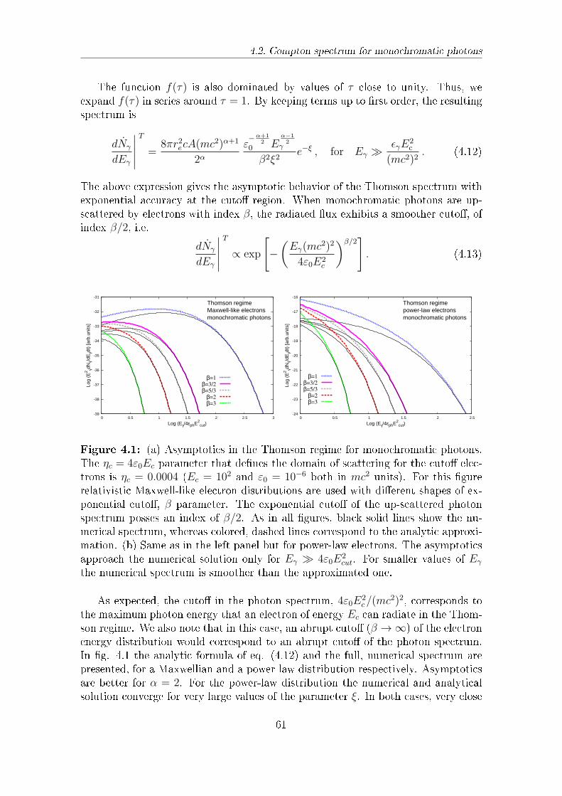
4.2. Compton spectrum for monochromatic photons
The function f(τ) is also dominated by values of τ close to unity. Thus, weexpand f(τ) in series around τ = 1. By keeping terms up to rst order, the resultingspectrum is
dNγ
dEγ
∣∣∣∣∣T
=8πr2ecA(mc2)α+1
2αε−α+1
20 E
α−12
γ
β2ξ2e−ξ , for Eγ ≫
ϵγE2c
(mc2)2. (4.12)
The above expression gives the asymptotic behavior of the Thomson spectrum withexponential accuracy at the cuto region. When monochromatic photons are up-scattered by electrons with index β, the radiated ux exhibits a smoother cuto, ofindex β/2, i.e.
dNγ
dEγ
∣∣∣∣∣T
∝ exp
[−(Eγ(mc2)2
4ε0E2c
)β/2]. (4.13)
-39
-38
-37
-36
-35
-34
-33
-32
-31
0 0.5 1 1.5 2 2.5 3
Log
(E2 γd
Nγ/
dEγd
t) [a
rb.u
nits
]
Log (Eγ/4εphE2cut)
Thomson regimeMaxwell-like electronsmonochromatic photons
β=1
β=3/2
β=5/3
β=2
β=3
-24
-23
-22
-21
-20
-19
-18
-17
-16
0 0.5 1 1.5 2 2.5
Log
(E2 γd
Nγ/
dEγd
t) [a
rb.u
nits
]
Log (Eγ/4εphE2cut)
Thomson regimepower-law electronsmonochromatic photons
β=1
β=3/2
β=5/3
β=2
β=3
Figure 4.1: (a) Asymptotics in the Thomson regime for monochromatic photons.The ηc = 4ε0Ec parameter that denes the domain of scattering for the cuto elec-trons is ηc = 0.0004 (Ec = 102 and ε0 = 10−6 both in mc2 units). For this gurerelativistic Maxwell-like electron distributions are used with dierent shapes of ex-ponential cuto, β parameter. The exponential cuto of the up-scattered photonspectrum posses an index of β/2. As in all gures, black solid lines show the nu-merical spectrum, whereas colored, dashed lines correspond to the analytic approxi-mation. (b) Same as in the left panel but for power-law electrons. The asymptoticsapproach the numerical solution only for Eγ ≫ 4ε0E
2cut. For smaller values of Eγ
the numerical spectrum is smoother than the approximated one.
As expected, the cuto in the photon spectrum, 4ε0E2c /(mc2)2, corresponds to
the maximum photon energy that an electron of energy Ec can radiate in the Thom-son regime. We also note that in this case, an abrupt cuto (β → ∞) of the electronenergy distribution would correspond to an abrupt cuto of the photon spectrum.In g. 4.1 the analytic formula of eq. (4.12) and the full, numerical spectrum arepresented, for a Maxwellian and a power-law distribution respectively. Asymptoticsare better for α = 2. For the power-law distribution the numerical and analyticalsolution converge for very large values of the parameter ξ. In both cases, very close
61
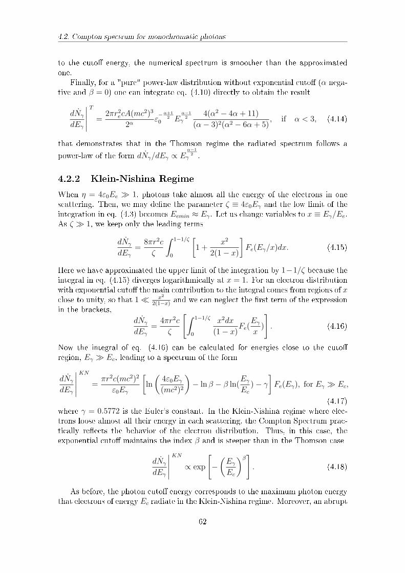
4.2. Compton spectrum for monochromatic photons
to the cuto energy, the numerical spectrum is smoother than the approximatedone.
Finally, for a "pure" power-law distribution without exponential cuto (α nega-tive and β = 0) one can integrate eq. (4.10) directly to obtain the result
dNγ
dEγ
∣∣∣∣∣T
=2πr2ecA(mc2)3
2αε−α+1
20 E
α−12
γ4(α2 − 4α + 11)
(α− 3)2(α2 − 6α + 5), if α < 3, (4.14)
that demonstrates that in the Thomson regime the radiated spectrum follows a
power-law of the form dNγ/dEγ ∝ Eα−12
γ .
4.2.2 Klein-Nishina Regime
When η = 4ε0Ee ≫ 1, photons take almost all the energy of the electrons in onescattering. Then, we may dene the parameter ζ ≡ 4ε0Eγ and the low limit of theintegration in eq. (4.3) becomes Eemin ≈ Eγ. Let us change variables to x ≡ Eγ/Ee.As ζ ≫ 1, we keep only the leading terms
dNγ
dEγ
=8πr2c
ζ
∫ 1−1/ζ
0
[1 +
x2
2(1− x)
]Fe(Eγ/x)dx. (4.15)
Here we have approximated the upper limit of the integration by 1−1/ζ because theintegral in eq. (4.15) diverges logarithmically at x = 1. For an electron distributionwith exponential cuto the main contribution to the integral comes from regions of xclose to unity, so that 1 ≪ x2
2(1−x) and we can neglect the rst term of the expressionin the brackets,
dNγ
dEγ
=4πr2c
ζ
[∫ 1−1/ζ
0
x2dx
(1− x)Fe(
Eγ
x)
]. (4.16)
Now the integral of eq. (4.16) can be calculated for energies close to the cutoregion, Eγ ≫ Ec, leading to a spectrum of the form
dNγ
dEγ
∣∣∣∣∣KN
=πr2c(mc2)2
ε0Eγ
[ln
(4ε0Eγ
(mc2)2
)− ln β − β ln(
Eγ
Ec
)− γ
]Fe(Eγ), for Eγ ≫ Ec,
(4.17)where γ = 0.5772 is the Euler's constant. In the Klein-Nishina regime where elec-trons loose almost all their energy in each scattering, the Compton Spectrum prac-tically reects the behavior of the electron distribution. Thus, in this case, theexponential cuto maintains the index β and is steeper than in the Thomson case
dNγ
dEγ
∣∣∣∣∣KN
∝ exp
[−(Eγ
Ec
)β]. (4.18)
As before, the photon cuto energy corresponds to the maximum photon energythat electrons of energy Ec radiate in the Klein-Nishina regime. Moreover, an abrupt
62
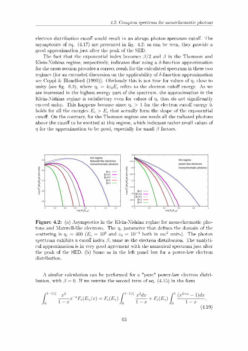
4.2. Compton spectrum for monochromatic photons
electron distribution cuto would result in an abrupt photon spectrum cuto. Theasymptotics of eq. (4.17) are presented in g. 4.2; as can be seen, they provide agood approximation just after the peak of the SED.
The fact that the exponential index becomes β/2 and β in the Thomson andKlein-Nishina regime, respectively, indicates that using a δ-function approximationfor the cross section provides a correct result for the calculated spectrum in these tworegimes (for an extended discussion on the applicability of δ-function approximationsee Coppi & Blandford (1990)). Obviously this is not true for values of ηc close tounity (see g. 6.3), where ηc = 4ε0Ec refers to the electron cuto energy. As weare interested in the highest energy part of the spectrum, the approximation in theKlein-Nishina regime is satisfactory even for values of ηc that do not signicantlyexceed unity. This happens because since ηc > 1 for the electron cuto energy itholds for all the energies Ee > Ec that actually form the shape of the exponentialcuto. On the contrary, for the Thomson regime one needs all the radiated photonsabove the cuto to be emitted at this regime, which indicates rather small values ofη for the approximation to be good, especially for small β factors.
-19
-18
-17
-16
-15
0 0.2 0.4 0.6 0.8 1 1.2 1.4
Log
(E2 γd
Nγ/
dEγd
t) [a
rb.u
nits
]
Log (Eγ/Ecut)
KN regimeMaxwell-like electronsmonochromatic photons
β=1
β=3/2
β=5/3
β=2
β=3
-19
-18.5
-18
-17.5
-17
-16.5
-16
-15.5
-15
0 0.2 0.4 0.6 0.8 1
Log
(E2 γd
Nγ/
dEγd
t) [a
rb.u
nits
]
Log (Eγ/Ecut)
KN regime
power-law electrons
monochromatic photons
β=1
β=3/2
β=5/3
β=2
β=3
Figure 4.2: (a) Asymptotics in the Klein-Nishina regime for monochromatic pho-tons and Maxwell-like electrons. The ηc parameter that denes the domain of thescattering is ηc = 400 (Ec = 106 and ε0 = 10−4 both in mc2 units). The photonspectrum exhibits a cuto index β, same as the electron distribution. The analyti-cal approximation is in very good agreement with the numerical spectrum just afterthe peak of the SED. (b) Same as in the left panel but for a power-law electrondistribution.
A similar calculation can be performed for a "pure" power-law electron distri-bution, with β = 0. If we rewrite the second term of eq. (4.15) in the form
∫ 1−1/ζ
0
x2
1− xx−aFe(Eγ/x) = Fe(Eγ)
∫ 1−1/ζ
0
x2dx
1− x+ Fe(Eγ)
∫ 1
0
(x2+α − 1)dx
1− x,
(4.19)
63
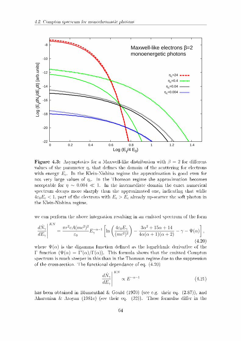
4.2. Compton spectrum for monochromatic photons
-22
-20
-18
-16
-14
-12
-10
-8
0 0.2 0.4 0.6 0.8 1 1.2 1.4
Log
(Eγd
Nγ/
dEγd
t) [a
rb.u
nits
]
Log (Eγ/4 E0)
Maxwell-like electrons β=2monoenergetic photons
ηc=24
ηc=0.4
ηc=0.04
ηc=0.004
Figure 4.3: Asymptotics for a Maxwell-like distribution with β = 2 for dierentvalues of the parameter ηc that denes the domain of the scattering for electronswith energy Ec. In the Klein-Nishina regime the approximation is good even fornot very large values of ηc. In the Thomson regime the approximation becomesacceptable for η ∼ 0.004 ≪ 1. In the intermediate domain the exact numericalspectrum decays more sharply than the approximated one, indicating that while4ε0Ec < 1, part of the electrons with Ee > Ec already up-scatter the soft photon inthe Klein-Nishina regime.
we can perform the above integration resulting in an emitted spectrum of the form
dNγ
dEγ
∣∣∣∣∣KN
=πr2cA(mc2)2
ε0E−α−1γ
[ln
(4ε0Eγ
(mc2)2
)− 3α2 + 15α + 14
4α(α + 1)(α + 2)− γ −Ψ(α)
],
(4.20)where Ψ(α) is the digamma function dened as the logarithmic derivative of theΓ function (Ψ(α) = Γ′(α)/Γ(α)). This formula shows that the emitted Comptonspectrum is much steeper in this than in the Thomson regime due to the suppressionof the cross-section. The functional dependance of eq. (4.20)
dNγ
dEγ
∣∣∣∣∣KN
∝ E−α−1 (4.21)
has been obtained in Blumenthal & Gould (1970) (see e.g. their eq. (2.87)), andAharonian & Atoyan (1981c) (see their eq. (32)). These formulas dier in the
64
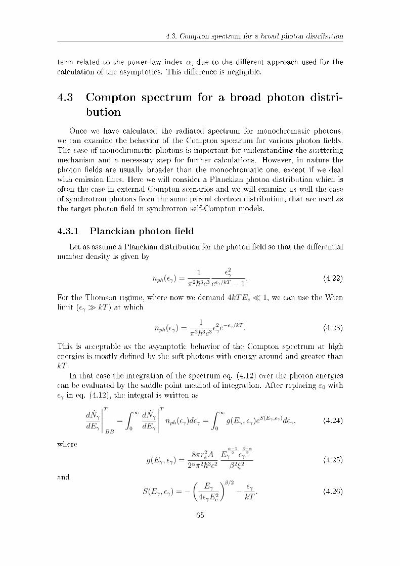
4.3. Compton spectrum for a broad photon distribution
term related to the power-law index α, due to the dierent approach used for thecalculation of the asymptotics. This dierence is negligible.
4.3 Compton spectrum for a broad photon distri-
bution
Once we have calculated the radiated spectrum for monochromatic photons,we can examine the behavior of the Compton spectrum for various photon elds.The case of monochromatic photons is important for understanding the scatteringmechanism and a necessary step for further calculations. However, in nature thephoton elds are usually broader than the monochromatic one, except if we dealwith emission lines. Here we will consider a Planckian photon distribution which isoften the case in external Compton scenarios and we will examine as well the caseof synchrotron photons from the same parent electron distribution, that are used asthe target photon eld in synchrotron self-Compton models.
4.3.1 Planckian photon eld
Let as assume a Planckian distribution for the photon eld so that the dierentialnumber density is given by
nph(ϵγ) =1
π2~3c3ϵ2γ
eϵγ/kT − 1. (4.22)
For the Thomson regime, where now we demand 4kTEe ≪ 1, we can use the Wienlimit (ϵγ ≫ kT ) at which
nph(ϵγ) =1
π2~3c3ϵ2γe
−ϵγ/kT . (4.23)
This is acceptable as the asymptotic behavior of the Compton spectrum at highenergies is mostly dened by the soft photons with energy around and greater thankT .
In that case the integration of the spectrum eq. (4.12) over the photon energiescan be evaluated by the saddle point method of integration. After replacing ε0 withϵγ in eq. (4.12), the integral is written as
dNγ
dEγ
∣∣∣∣∣T
BB
=
∫ ∞
0
dNγ
dEγ
∣∣∣∣∣T
nph(ϵγ)dϵγ =
∫ ∞
0
g(Eγ, ϵγ)eS(Eγ ,ϵγ)dϵγ, (4.24)
where
g(Eγ, ϵγ) =8πr2eA
2απ2~3c2E
α−12
γ ϵ3−α2
γ
β2ξ2(4.25)
and
S(Eγ, ϵγ) = −(
Eγ
4ϵγE2c
)β/2− ϵγ
kT. (4.26)
65
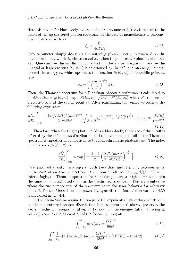
4.3. Compton spectrum for a broad photon distribution
Here BB stands for black body. Let as dene the parameter ξ1 that is related to thecuto of the up-scattered photon spectrum for the case of monochromatic photons,if we replace ϵγ with kT
ξ1 ≡Eγ
4kTE2c
. (4.27)
This parameter simply describes the outgoing photon energy normalized to themaximum energy which Ec electrons radiate when they up-scatter photons of energykT . One can use the saddle point method for the above integration because theintegral at large energies (ξ1 ≫ 1) is determined by the soft photon energy intervalaround the energy x0 which optimizes the function S(Eγ, ϵγ). The saddle point x0
is at
x0 =β
2
(2ξ1β
) ββ+2
kT. (4.28)
Then, the Thomson spectrum for a Planckian photon distribution is calculated tobe dNγ/dEγ = g(Eγ, ϵ∗) exp[−S(Eγ, x0)]
√2π/− S ′′(Eγ, x0) where S ′′ the second
derivative of S at the saddle point x0. After rearranging the terms, we retrieve thefollowing expression
dNγ
dEγ
∣∣∣∣∣T
BB
=4πr2eA(kT )
52 (mc2)α+1
2απ2~3c2
√π
β + 2x−α
20 E
α−12
γ e−β+22 ( 2ξ1
β )β
β+2
, for Eγ ≫4kTE2
c
(mc2)2,
(4.29)Therefore, when the target photon eld is a black-body, the shape of the cuto is
aected by the soft photon distribution and the exponential cuto in the Thomsonspectrum is smoother in comparison to the monochromatic photons case. The indexnow becomes β/(β + 2) as
dNγ
dEγ
∣∣∣∣∣T
BB
∝ exp[− β + 2
2
(2
β
Eγ(mc2)2
4kTE2c
) ββ+2 ]
. (4.30)
This exponential cuto is always smooth (less than unity) and it becomes unityin the case of an abrupt electron distribution cuto, as limβ→∞ β/(β + 2) = 1.Interestingly, the Thomson spectrum for Planckian photons at high energies exhibitsthe same exponential cuto shape as the synchrotron spectrum. This is the only casewhere the two components of the spectrum show the same behavior for arbitraryindex β. For the Maxwellian and power-law type distributions of electrons, eq. 4.30is presented in g. 4.4.
In the Klein-Nishina regime the shape of the exponential cuto does not dependon the up-scattered photon distribution but, as mentioned above, preserves theelectron index β. Integration of eq. (4.17) over photon energies (after replacing ε0with ϵγ) requires the calculation of the following integrals∫ ∞
0
1
ϵγn(ϵγ)dϵγ =
(kT )2
6~c3, (4.31)∫ ∞
0
1
ϵγn(ϵγ) ln (4ϵγEγ)dϵγ =
(kT )2
6~c3(ln (4kTEγ)− 0.1472) . (4.32)
66
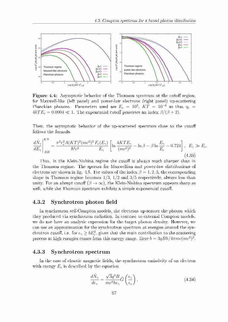
4.3. Compton spectrum for a broad photon distribution
-24
-23
-22
-21
-20
0 0.5 1 1.5 2 2.5 3
Log
(E2 γd
Nγ/
dEγd
t) [a
rb.u
nits
]
Log (Eγ/4KT E2cut)
Thomson regime
Maxwell-like electrons
Planckian photons
β=1
β=3/2
β=5/3
β=2
β=3
-10
-9
-8
-7
-6
-5
0 0.5 1 1.5 2 2.5 3
Log
(E2 γd
Nγ/
dEγd
t) [a
rb.u
nits
]
Log (Eγ/4KT E2cut)
Thomson regime
power-law electrons
Planckian photons
β=1
β=3/2
β=5/3
β=2
β=3
Figure 4.4: Asymptotic behavior of the Thomson spectrum at the cuto region,for Maxwell-like (left panel) and power-law electrons (right panel) up-scatteringPlanckian photons. Parameters used are Ec = 102, KT = 10−6 so that ηc =4kTEc = 0.0004 ≪ 1. The exponential cuto possesses an index β/(β + 2).
Then, the asymptotic behavior of the up-scattered spectrum close to the cutofollows the formula
dNγ
dEγ
∣∣∣∣∣KN
BB
=π2r2eA(KT )2(mc2)2
~3c2Fe(Eγ)
Eγ
[ln
4KTEγ
(mc2)2− ln β − β ln
Eγ
Ec
− 0.724
], Eγ ≫ Ec.
(4.33)Thus, in the Klein-Nishina regime the cuto is always much sharper than in
the Thomson regime. The spectra for Maxwellian and power-law distributions ofelectrons are shown in g. 4.5. For values of the index β = 1, 2, 3, the correspondingshape in Thomson regime becomes 1/3, 1/2 and 3/5 respectively, always less thanunity. For an abrupt cuto (β → ∞), the Klein-Nishina spectrum appears sharp aswell, while the Thomson spectrum exhibits a simple exponential cuto.
4.3.2 Synchrotron photon eld
In synchrotron self-Compton models, the electrons up-scatter the photon whichthey produced via synchrotron radiation. In contrast to external Compton models,we do not have an analytic expression for the target photon density. However, wecan use an approximation for the synchrotron spectrum at energies around the syn-chrotron cuto, i.e. for ϵγ ≥ bE2
c , given that the main contribution to the scatteringprocess at high energies comes from this energy range. Here b = 3qBh/4πmc(mc2)2.
4.3.3 Synchrotron spectrum
In the case of chaotic magnetic elds, the synchrotron emissivity of an electronwith energy Ee is described by the equation
dNγ
dϵγ=
√3q3B
mc2hϵγG
(ϵγϵs
), (4.34)
67
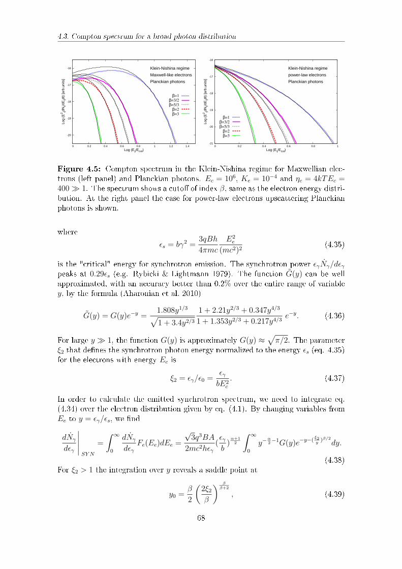
4.3. Compton spectrum for a broad photon distribution
-20
-19
-18
-17
-16
0 0.2 0.4 0.6 0.8 1 1.2 1.4
Log
(E2 γd
Nγ/
dEγd
t) [a
rb.u
nits
]
Log (Eγ/Ecut)
Klein-Nishina regime
Maxwell-like electrons
Planckian photons
β=1
β=3/2
β=5/3
β=2
β=3
-21
-20
-19
-18
-17
-16
0 0.2 0.4 0.6 0.8 1
Log
(E2 γd
Nγ/
dEγd
t) [a
rb.u
nits
]
Log (Eγ/Ecut)
Klein-Nishina regime
power-law electrons
Planckian photons
β=1
β=3/2
β=5/3
β=2
β=3
Figure 4.5: Compton spectrum in the Klein-Nishina regime for Maxwellian elec-trons (left panel) and Planckian photons. Ec = 106, Ke = 10−4 and ηc = 4kTEc =400 ≫ 1. The spectrum shows a cuto of index β, same as the electron energy distri-bution. At the right panel the case for power-law electrons upscattering Planckianphotons is shown.
where
ϵs = bγ2 =3qBh
4πmc
E2e
(mc2)2(4.35)
is the "critical" energy for synchrotron emission. The synchrotron power ϵγNγ/dϵγpeaks at 0.29ϵs (e.g. Rybicki & Lightmann 1979). The function G(y) can be wellapproximated, with an accuracy better than 0.2% over the entire range of variabley, by the formula (Aharonian et al. 2010)
G(y) = G(y)e−y =1.808y1/3√1 + 3.4y2/3
1 + 2.21y2/3 + 0.347y4/3
1 + 1.353y2/3 + 0.217y4/3e−y. (4.36)
For large y ≫ 1, the function G(y) is approximately G(y) ≈√
π/2. The parameterξ2 that denes the synchrotron photon energy normalized to the energy ϵs (eq. 4.35)for the electrons with energy Ec is
ξ2 = ϵγ/ϵ0 =ϵγbE2
c
. (4.37)
In order to calculate the emitted synchrotron spectrum, we need to integrate eq.(4.34) over the electron distribution given by eq. (4.1). By changing variables fromEe to y = ϵγ/ϵs, we nd
dNγ
dϵγ
∣∣∣∣∣SY N
=
∫ ∞
0
dNγ
dϵγFe(Ee)dEe =
√3q3BA
2mc2hϵγ(ϵγb)α+12
∫ ∞
0
y−α2−1G(y)e−y−(
ξ2y)β/2dy.
(4.38)For ξ2 > 1 the integration over y reveals a saddle point at
y0 =β
2
(2ξ2β
) ββ+2
, (4.39)
68
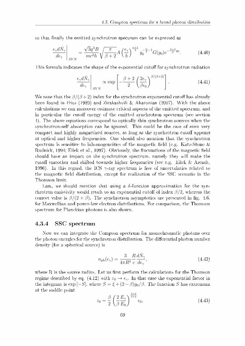
4.3. Compton spectrum for a broad photon distribution
so that nally the emitted synchrotron spectrum can be expressed as
ϵγdNγ
dϵγ
∣∣∣∣∣SY N
=
√3q3B
mc2h
√π
β + 2A(ϵγb
)α+12
y−α
2−1
0 G(y0)e− 2+β
βy0 . (4.40)
This formula indicates the shape of the exponential cuto for synchrotron radiation
ϵγdNγ
dϵγ
∣∣∣∣∣SY N
∝ exp
[−β + 2
2
(2ϵγβϵ0
)β/(β+2)]. (4.41)
We note that the β/(β+2) index for the synchrotron exponential cuto has alreadybeen found in Fritz (1989) and Zirakashvili & Aharonian (2007). With the abovecalculations we can moreover estimate critical aspects of the emitted spectrum, andin particular the cuto energy of the emitted synchrotron spectrum (see section4). The above equations correspond to optically thin synchrotron sources when thesynchrotron-self absorption can be ignored. This could be the case of even verycompact and highly magnetized sources, as long as the synchrotron cuto appearsat optical and higher frequencies. One should also mention that the synchrotronspectrum is sensitive to inhomogeneities of the magnetic eld (e.g. Katz-Stone &Rudnick, 1994; Eilek et al., 1997). Obviously, the uctuations of the magnetic eldshould have an impact on the synchrotron spectrum, namely they will make thecuto smoother and shifted towards higher frequencies (see e.g. Eilek & Arendt,1996). In this regard, the ICS γ-ray spectrum is free of uncertainties related tothe magnetic eld distribution, except for realization of the SSC scenario in theThomson limit.
Last, we should mention that using a δ-function approximation for the syn-chrotron emissivity would result to an exponential cuto of index β/2, whereas thecorrect value is β/(2 + β). The synchrotron asymptotics are presented in g. 4.6,for Maxwellian and power-law electron distributions. For comparison, the Thomsonspectrum for Planckian photons is also shown.
4.3.4 SSC spectrum
Now we can integrate the Compton spectrum for monochromatic photons overthe photon energies for the synchrotron distribution. The dierential photon numberdensity (for a spherical source) is
nph(ϵγ) =3
4πR3
R
c
dNγ
dϵγ, (4.42)
where R is the source radius. Let us rst perform the calculations for the Thomsonregime described by eq. (4.12) with ε0 → ϵγ. In that case the exponential factor inthe integrant is exp [−S], where S = ξ+(2−β)y0/β. The function S has extremumat the saddle point
z0 =β
2
(2
β
Eγ
E0
)β+2β+4
ϵ0, (4.43)
69
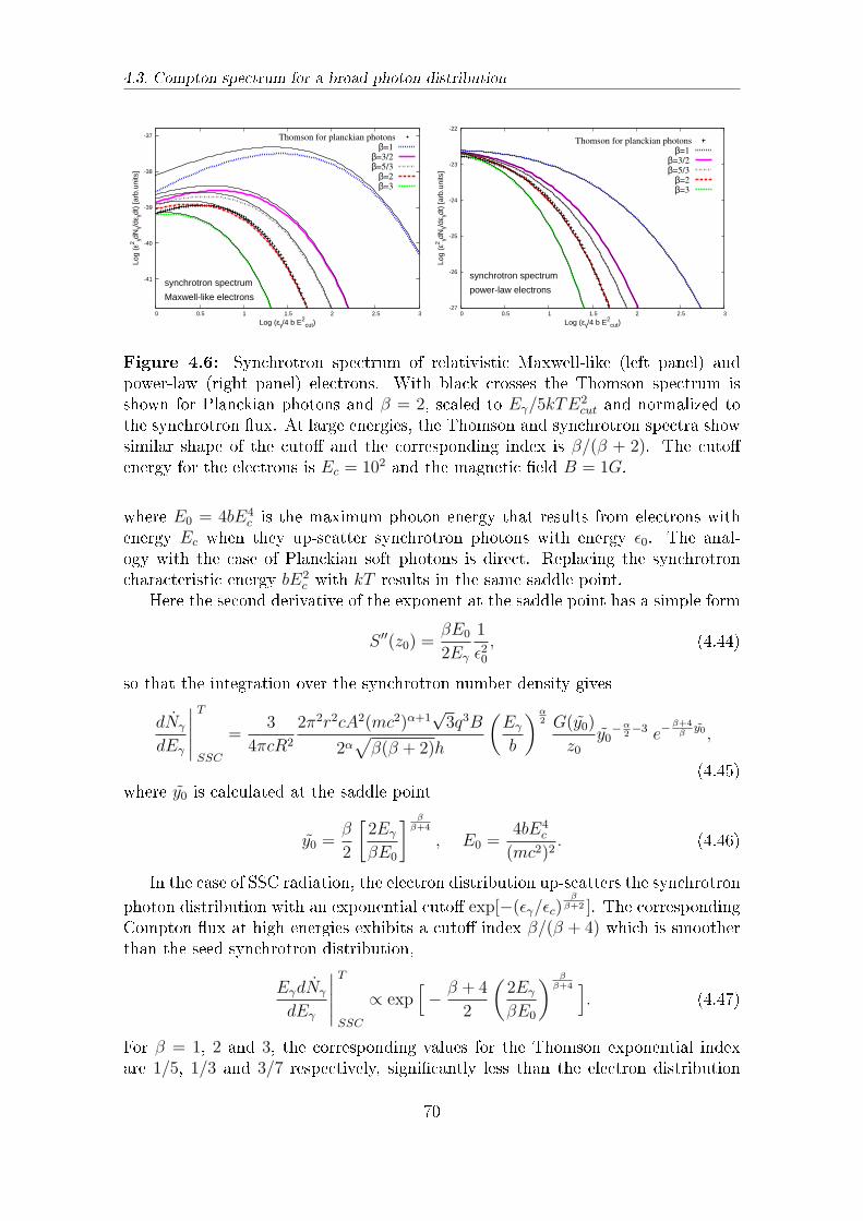
4.3. Compton spectrum for a broad photon distribution
-41
-40
-39
-38
-37
0 0.5 1 1.5 2 2.5 3
Log
(ε2 γd
Nγ/
dεγd
t) [a
rb.u
nits
]
Log (εγ/4 b E2cut)
synchrotron spectrum
Maxwell-like electrons
Thomson for planckian photonsβ=1
β=3/2 β=5/3
β=2 β=3
-27
-26
-25
-24
-23
-22
0 0.5 1 1.5 2 2.5 3
Log
(ε2 γd
Nγ/
dεγd
t) [a
rb.u
nits
]
Log (εγ/4 b E2cut)
synchrotron spectrum
power-law electrons
Thomson for planckian photonsβ=1
β=3/2 β=5/3
β=2 β=3
Figure 4.6: Synchrotron spectrum of relativistic Maxwell-like (left panel) andpower-law (right panel) electrons. With black crosses the Thomson spectrum isshown for Planckian photons and β = 2, scaled to Eγ/5kTE
2cut and normalized to
the synchrotron ux. At large energies, the Thomson and synchrotron spectra showsimilar shape of the cuto and the corresponding index is β/(β + 2). The cutoenergy for the electrons is Ec = 102 and the magnetic eld B = 1G.
where E0 = 4bE4c is the maximum photon energy that results from electrons with
energy Ec when they up-scatter synchrotron photons with energy ϵ0. The anal-ogy with the case of Planckian soft photons is direct. Replacing the synchrotroncharacteristic energy bE2
c with kT results in the same saddle point.Here the second derivative of the exponent at the saddle point has a simple form
S ′′(z0) =βE0
2Eγ
1
ϵ20, (4.44)
so that the integration over the synchrotron number density gives
dNγ
dEγ
∣∣∣∣∣T
SSC
=3
4πcR2
2π2r2cA2(mc2)α+1√3q3B
2α√β(β + 2)h
(Eγ
b
)α2 G(y0)
z0y0
−α2−3 e−
β+4βy0 ,
(4.45)where y0 is calculated at the saddle point
y0 =β
2
[2Eγ
βE0
] ββ+4
, E0 =4bE4
c
(mc2)2. (4.46)
In the case of SSC radiation, the electron distribution up-scatters the synchrotron
photon distribution with an exponential cuto exp[−(ϵγ/ϵc)β
β+2 ]. The correspondingCompton ux at high energies exhibits a cuto index β/(β + 4) which is smootherthan the seed synchrotron distribution,
EγdNγ
dEγ
∣∣∣∣∣T
SSC
∝ exp[− β + 4
2
(2Eγ
βE0
) ββ+4 ]
. (4.47)
For β = 1, 2 and 3, the corresponding values for the Thomson exponential indexare 1/5, 1/3 and 3/7 respectively, signicantly less than the electron distribution
70
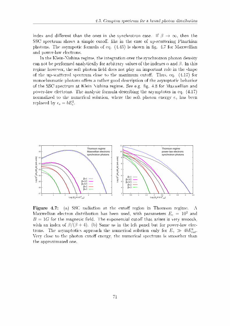
4.3. Compton spectrum for a broad photon distribution
index and dierent than the ones in the synchrotron case. If β → ∞, then theSSC spectrum shows a simple cuto, like in the case of up-scattering Planckianphotons. The asympotic formula of eq. (4.45) is shown in g. 4.7 for Maxwellianand power-law electrons.
In the Klein-Nishina regime, the integration over the synchrotron photon densitycan not be performed analytically for arbitrary values of the indexes α and β. In thisregime however, the soft photon eld does not play an important role in the shapeof the up-scattered spectrum close to the maximum cuto. Thus, eq. (4.17) formonochromatic photons oers a rather good description of the asymptotic behaviorof the SSC spectrum at Klein-Nishina regime. See e.g. g. 4.8 for Maxwellian andpower-law electrons. The analytic formula describing the asymptotes in eq. (4.17)normalized to the numerical solution, where the soft photon energy ϵγ has beenreplaced by ϵs = bE2
c .
-27
-26
-25
-24
-23
-22
-21
-20
-19
0 1 2 3 4 5 6
Log
(E2 γd
Nγ/
dEγd
t) [a
rb.u
nits
]
Log (Eγ/4 b E4cut)
Thomson regimeMawxellian electronssynchrotron photons
β=1
β=3/2
β=5/3
β=2
β=3
3
4
5
6
7
8
9
10
11
0 0.5 1 1.5 2 2.5 3 3.5 4 4.5
Log
(E2 γd
Nγ/
dEγd
t) [a
rb.u
nits
]
Log (Eγ/4 b E4cut)
Thomson regimepower-law electronssynchrotron photons
β=1
β=3/2
β=5/3
β=2
β=3
Figure 4.7: (a) SSC radiation at the cuto region in Thomson regime. AMaxwellian electron distribution has been used, with parameters Ec = 102 andB = 1G for the magnetic eld. The exponential cuto that arises is very smooth,with an index of β/(β + 4). (b) Same as in the left panel but for power-law elec-trons. The asymptotics approach the numerical solution only for Eγ ≫ 4bE4
cut.Very close to the photon cuto energy, the numerical spectrum is smoother thanthe approximated one.
71
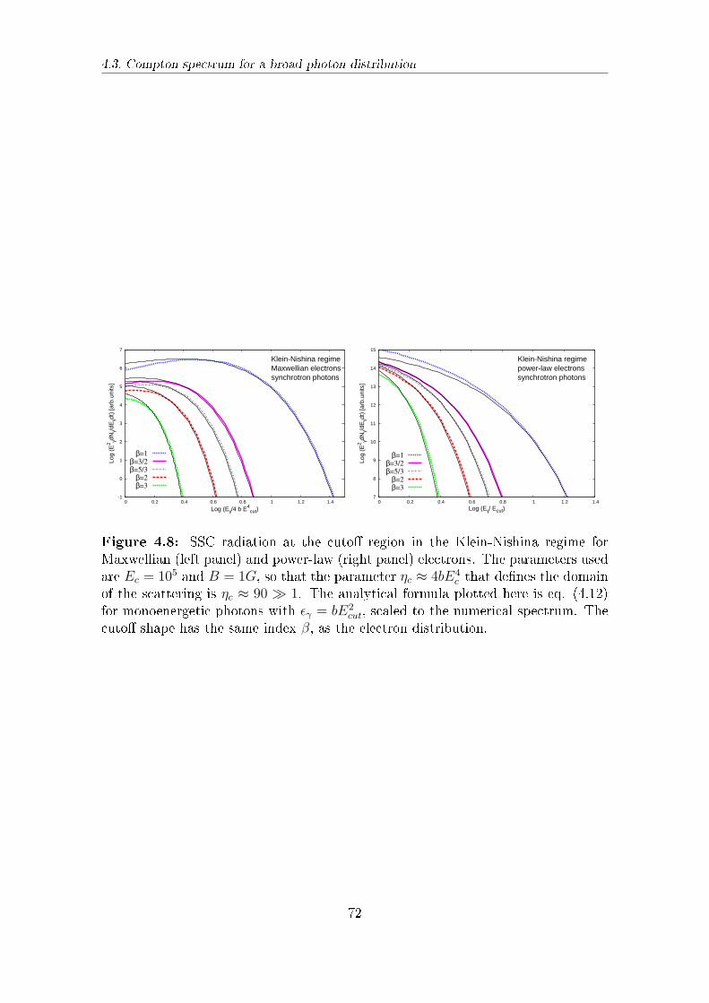
4.3. Compton spectrum for a broad photon distribution
-1
0
1
2
3
4
5
6
7
0 0.2 0.4 0.6 0.8 1 1.2 1.4
Log
(E2 γd
Nγ/
dEγd
t) [a
rb.u
nits
]
Log (Eγ/4 b E4cut)
Klein-Nishina regimeMaxwellian electronssynchrotron photons
β=1
β=3/2
β=5/3
β=2
β=3
7
8
9
10
11
12
13
14
15
0 0.2 0.4 0.6 0.8 1 1.2 1.4
Log
(E2 γd
Nγ/
dEγd
t) [a
rb.u
nits
]
Log (Eγ/ Ecut)
Klein-Nishina regimepower-law electronssynchrotron photons
β=1
β=3/2
β=5/3
β=2
β=3
Figure 4.8: SSC radiation at the cuto region in the Klein-Nishina regime forMaxwellian (left panel) and power-law (right panel) electrons. The parameters usedare Ec = 105 and B = 1G, so that the parameter ηc ≈ 4bE4
c that denes the domainof the scattering is ηc ≈ 90 ≫ 1. The analytical formula plotted here is eq. (4.12)for monoenergetic photons with ϵγ = bE2
cut, scaled to the numerical spectrum. Thecuto shape has the same index β, as the electron distribution.
72
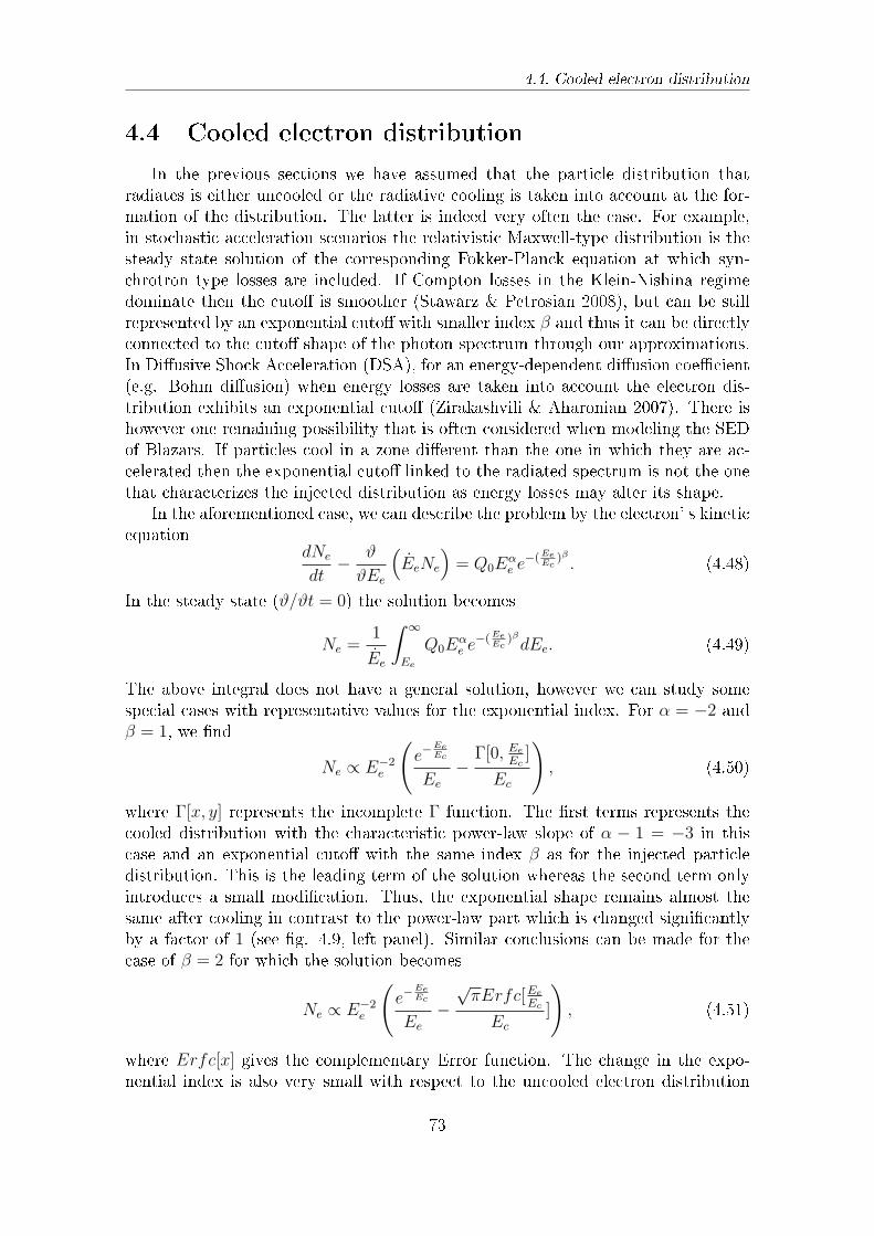
4.4. Cooled electron distribution
4.4 Cooled electron distribution
In the previous sections we have assumed that the particle distribution thatradiates is either uncooled or the radiative cooling is taken into account at the for-mation of the distribution. The latter is indeed very often the case. For example,in stochastic acceleration scenarios the relativistic Maxwell-type distribution is thesteady state solution of the corresponding Fokker-Planck equation at which syn-chrotron type losses are included. If Compton losses in the Klein-Nishina regimedominate then the cuto is smoother (Stawarz & Petrosian 2008), but can be stillrepresented by an exponential cuto with smaller index β and thus it can be directlyconnected to the cuto shape of the photon spectrum through our approximations.In Diusive Shock Acceleration (DSA), for an energy-dependent diusion coecient(e.g. Bohm diusion) when energy losses are taken into account the electron dis-tribution exhibits an exponential cuto (Zirakashvili & Aharonian 2007). There ishowever one remaining possibility that is often considered when modeling the SEDof Blazars. If particles cool in a zone dierent than the one in which they are ac-celerated then the exponential cuto linked to the radiated spectrum is not the onethat characterizes the injected distribution as energy losses may alter its shape.
In the aforementioned case, we can describe the problem by the electron' s kineticequation
dNe
dt− ϑ
ϑEe
(EeNe
)= Q0E
αe e
−(EeEc
)β . (4.48)
In the steady state (ϑ/ϑt = 0) the solution becomes
Ne =1
Ee
∫ ∞
Ee
Q0Eαe e
−(EeEc
)βdEe. (4.49)
The above integral does not have a general solution, however we can study somespecial cases with representative values for the exponential index. For α = −2 andβ = 1, we nd
Ne ∝ E−2e
(e−
EeEc
Ee
−Γ[0, Ee
Ec]
Ec
), (4.50)
where Γ[x, y] represents the incomplete Γ function. The rst terms represents thecooled distribution with the characteristic power-law slope of α − 1 = −3 in thiscase and an exponential cuto with the same index β as for the injected particledistribution. This is the leading term of the solution whereas the second term onlyintroduces a small modication. Thus, the exponential shape remains almost thesame after cooling in contrast to the power-law part which is changed signicantlyby a factor of 1 (see g. 4.9, left panel). Similar conclusions can be made for thecase of β = 2 for which the solution becomes
Ne ∝ E−2e
(e−
EeEc
Ee
−√πErfc[Ee
Ec
Ec
]
), (4.51)
where Erfc[x] gives the complementary Error function. The change in the expo-nential index is also very small with respect to the uncooled electron distribution
73
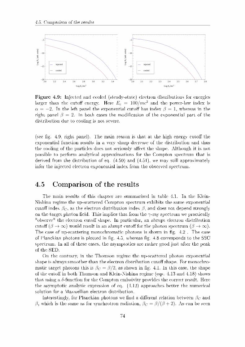
4.5. Comparison of the results
2.0 2.2 2.4 2.6 2.8 3.0 3.2 3.4-20
-15
-10
-5
Log Eemc2
Log
Ne@a
rb.u
nitsD
cooled
injected
2.0 2.1 2.2 2.3 2.4 2.5 2.6 2.7 2.8-20
-15
-10
-5
Log Eemc2
Log
Ne@a
rb.u
nitsD
cooled
injected
Figure 4.9: Injected and cooled (steady-state) electron distributions for energieslarger than the cuto energy. Here Ec = 100/mc2 and the power-law index isα = −2. In the left panel the exponential cuto has index β = 1, whereas in theright panel β = 2. In both cases the modication of the exponential part of thedistribution due to cooling is not severe.
(see g. 4.9, right panel). The main reason is that at the high energy cuto theexponential function results in a very sharp decrease of the distribution and thusthe cooling of the particles does not seriously aect the shape. Although it is notpossible to perform analytical approximations for the Compton spectrum that isderived from the distribution of eq. (4.50) and (4.51), we may still approximatelyinfer the injected electron exponential index from the observed spectrum.
4.5 Comparison of the results
The main results of this chapter are summarized in table 4.1. In the Klein-Nishina regime the up-scattered Compton spectrum exhibits the same exponentialcuto index βC , as the electron distribution index β, and does not depend stronglyon the target photon eld. This implies that from the γ-ray spectrum we practically"observe" the electron cuto shape. In particular, an abrupt electron distributioncuto (β → ∞) would result in an abrupt cuto for the photon spectrum (β → ∞).The case of up-scattering monochromatic photons is shown in g. 4.2 . The caseof Planckian photons is plotted in g. 4.5, whereas g. 4.8 corresponds to the SSCspectrum. In all of these cases, the asymptotics are rather good just after the peakof the SED.
On the contrary, in the Thomson regime the up-scattered photon exponentialshape is always smoother than the electron distribution cuto shape. For monochro-matic target photons this is βC = β/2, as shown in g. 4.1. In this case, the shapeof the cuto in both Thomson and Klein-Nishina regime (eqs. 4.13 and 4.18) showsthat using a δ-function for the Compton emissivity provides the correct result. Herethe asymptotic analytic expression of eq. (4.12) approaches better the numericalsolution for a Maxwellian electron distribution.
Interestingly, for Planckian photons we nd a dierent relation between βC andβ, which is the same as for synchrotron radiation, βC = β/(β + 2). As can be seen
74
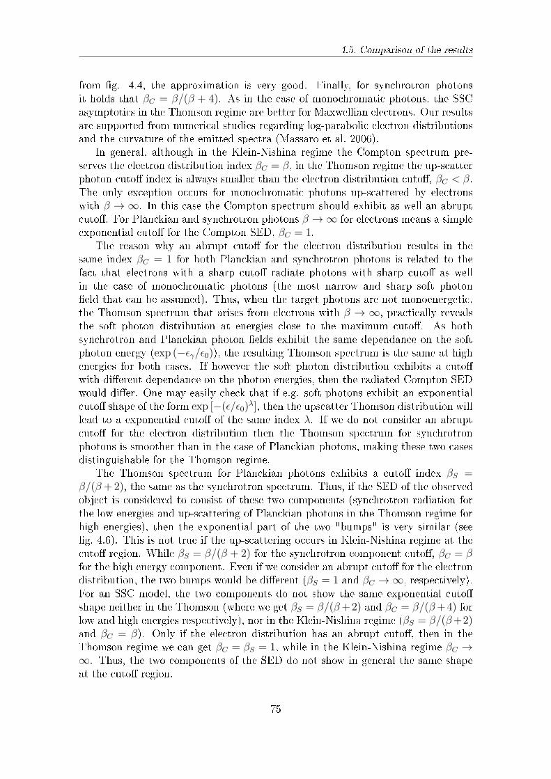
4.5. Comparison of the results
from g. 4.4, the approximation is very good. Finally, for synchrotron photonsit holds that βC = β/(β + 4). As in the case of monochromatic photons, the SSCasymptotics in the Thomson regime are better for Maxwellian electrons. Our resultsare supported from numerical studies regarding log-parabolic electron distributionsand the curvature of the emitted spectra (Massaro et al. 2006).
In general, although in the Klein-Nishina regime the Compton spectrum pre-serves the electron distribution index βC = β, in the Thomson regime the up-scatterphoton cuto index is always smaller than the electron distribution cuto, βC < β.The only exception occurs for monochromatic photons up-scattered by electronswith β → ∞. In this case the Compton spectrum should exhibit as well an abruptcuto. For Planckian and synchrotron photons β → ∞ for electrons means a simpleexponential cuto for the Compton SED, βC = 1.
The reason why an abrupt cuto for the electron distribution results in thesame index βC = 1 for both Planckian and synchrotron photons is related to thefact that electrons with a sharp cuto radiate photons with sharp cuto as wellin the case of monochromatic photons (the most narrow and sharp soft photoneld that can be assumed). Thus, when the target photons are not monoenergetic,the Thomson spectrum that arises from electrons with β → ∞, practically revealsthe soft photon distribution at energies close to the maximum cuto. As bothsynchrotron and Planckian photon elds exhibit the same dependance on the softphoton energy (exp (−ϵγ/ϵ0)), the resulting Thomson spectrum is the same at highenergies for both cases. If however the soft photon distribution exhibits a cutowith dierent dependance on the photon energies, then the radiated Compton SEDwould dier. One may easily check that if e.g. soft photons exhibit an exponentialcuto shape of the form exp [−(ϵ/ϵ0)
λ], then the upscatter Thomson distribution willlead to a exponential cuto of the same index λ. If we do not consider an abruptcuto for the electron distribution then the Thomson spectrum for synchrotronphotons is smoother than in the case of Planckian photons, making these two casesdistinguishable for the Thomson regime.
The Thomson spectrum for Planckian photons exhibits a cuto index βS =β/(β+2), the same as the synchrotron spectrum. Thus, if the SED of the observedobject is considered to consist of these two components (synchrotron radiation forthe low energies and up-scattering of Planckian photons in the Thomson regime forhigh energies), then the exponential part of the two "bumps" is very similar (seeg. 4.6). This is not true if the up-scattering occurs in Klein-Nishina regime at thecuto region. While βS = β/(β + 2) for the synchrotron component cuto, βC = βfor the high energy component. Even if we consider an abrupt cuto for the electrondistribution, the two bumps would be dierent (βS = 1 and βC → ∞, respectively).For an SSC model, the two components do not show the same exponential cutoshape neither in the Thomson (where we get βS = β/(β+2) and βC = β/(β+4) forlow and high energies respectively), nor in the Klein-Nishina regime (βS = β/(β+2)and βC = β). Only if the electron distribution has an abrupt cuto, then in theThomson regime we can get βC = βS = 1, while in the Klein-Nishina regime βC →∞. Thus, the two components of the SED do not show in general the same shapeat the cuto region.
75
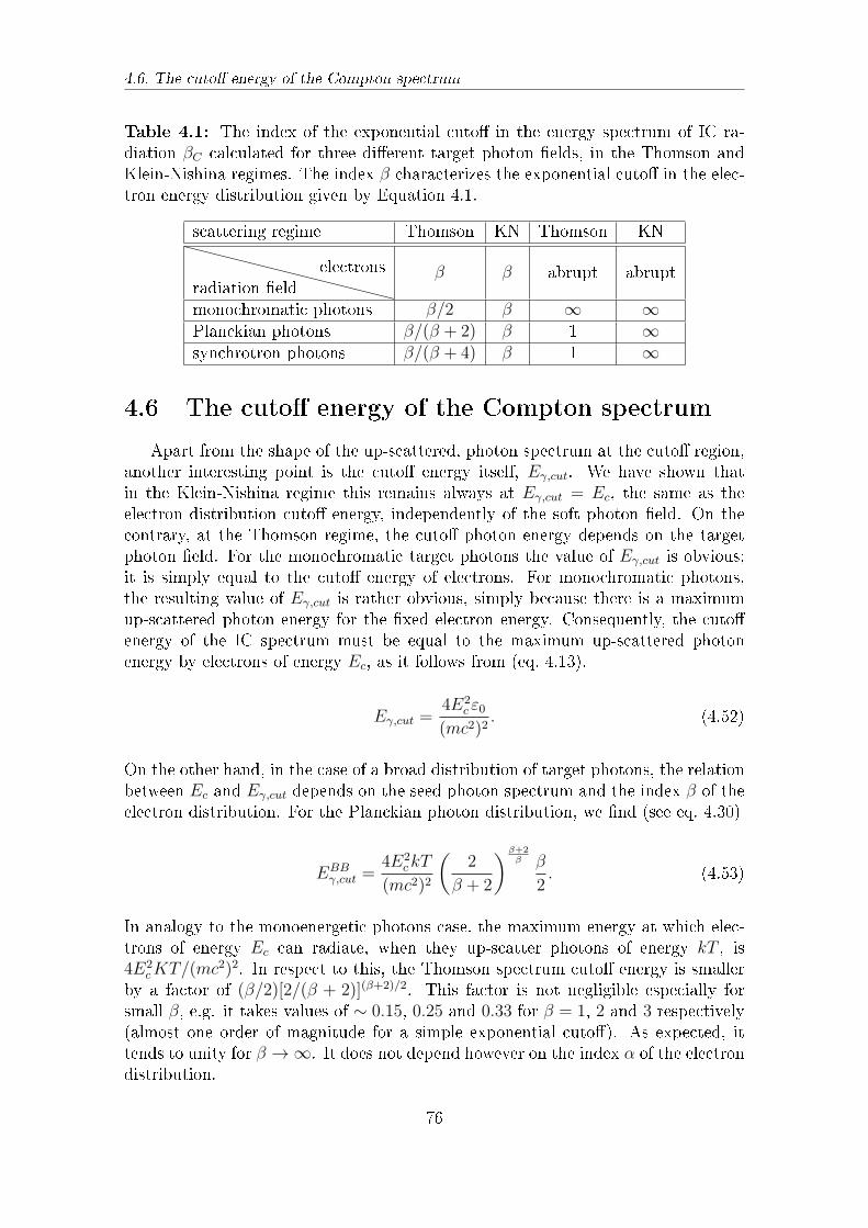
4.6. The cuto energy of the Compton spectrum
Table 4.1: The index of the exponential cuto in the energy spectrum of IC ra-diation βC calculated for three dierent target photon elds, in the Thomson andKlein-Nishina regimes. The index β characterizes the exponential cuto in the elec-tron energy distribution given by Equation 4.1.
scattering regime Thomson KN Thomson KN
radiation eldelectrons β β abrupt abrupt
monochromatic photons β/2 β ∞ ∞Planckian photons β/(β + 2) β 1 ∞synchrotron photons β/(β + 4) β 1 ∞
4.6 The cuto energy of the Compton spectrum
Apart from the shape of the up-scattered, photon spectrum at the cuto region,another interesting point is the cuto energy itself, Eγ,cut. We have shown thatin the Klein-Nishina regime this remains always at Eγ,cut = Ec, the same as theelectron distribution cuto energy, independently of the soft photon eld. On thecontrary, at the Thomson regime, the cuto photon energy depends on the targetphoton eld. For the monochromatic target photons the value of Eγ,cut is obvious;it is simply equal to the cuto energy of electrons. For monochromatic photons,the resulting value of Eγ,cut is rather obvious, simply because there is a maximumup-scattered photon energy for the xed electron energy. Consequently, the cutoenergy of the IC spectrum must be equal to the maximum up-scattered photonenergy by electrons of energy Ec, as it follows from (eq. 4.13),
Eγ,cut =4E2
c ε0(mc2)2
. (4.52)
On the other hand, in the case of a broad distribution of target photons, the relationbetween Ec and Eγ,cut depends on the seed photon spectrum and the index β of theelectron distribution. For the Planckian photon distribution, we nd (see eq. 4.30)
EBBγ,cut =
4E2ckT
(mc2)2
(2
β + 2
)β+2β β
2. (4.53)
In analogy to the monoenergetic photons case, the maximum energy at which elec-trons of energy Ec can radiate, when they up-scatter photons of energy kT , is4E2
cKT/(mc2)2. In respect to this, the Thomson spectrum cuto energy is smallerby a factor of (β/2)[2/(β + 2)](β+2)/2. This factor is not negligible especially forsmall β, e.g. it takes values of ∼ 0.15, 0.25 and 0.33 for β = 1, 2 and 3 respectively(almost one order of magnitude for a simple exponential cuto). As expected, ittends to unity for β → ∞. It does not depend however on the index α of the electrondistribution.
76
4.7. Summary
For synchrotron radiation, from eq. (4.41), we nd the cuto energy
ϵSY Nγ,cut = bE2c
(2
β + 2
)β+2β β
2, (4.54)
which reveals exactly the same factor as in the case of Thomson spectrum for Planck-ian photons, but now in respect to the characteristic energy bE2
c .Finally, for the case of SSC, eq. (4.47) gives
ESSCγ,cut =
4bE4c
(mc2)2
(2
β + 4
)β+4β β
2=
4E2c ϵ
SY Nγ,cut
(mc2)2
(2
β + 4
)β+4β(β + 2
2
)β+2β
(4.55)
If we compare the cuto energy with e.g. 4bE2cut ϵ
SY Nγ,cut/(mc2)2 then the factor related
to the index β takes values of ∼ 0.035, 0.15 and 0.25 for β = 1, 2 and 3, which areslightly less than in the case of a Planckian target photon eld. This is due tothe fact that the cuto shape is now smoother. These analytic results are usefulwhen modeling the observed spectrum, as one may infer the electron distributioncuto energy from the photon spectrum cuto energy with only the uncertaintyintroduced by a (possible) Doppler boosting. The position and the amplitude ofthe synchrotron and IC peaks in the SED contain very important information aboutphysical parameters of non-thermal sources, like the strength of the average magneticeld and the energy density of relativistic electrons. The shape of the SED, especiallyin the region of the cutos of the synchrotron and IC components of radiation,provide additional, more detailed information about the distributions of electronsand magnetic elds. For example, the spectral cuto in the IC component formed inthe the Klein-Nishina regime provides direct, model-independent information aboutthe energy spectrum of the highest energy electrons. This is a critical issue forunderstanding the particle acceleration mechanisms. Furthermore, combined withthe shape of the synchrotron cuto, it allows us to extract information about thedistribution of the magnetic eld. This can be demonstrated by the following simpleexample. Let as assume that we have observed a smooth synchrotron cuto whichcan be interpreted as the result of an electron distribution with an exponential indexe.g. β ≈ 1. This hypothesis can be checked by the shape of the cuto of the ICcomponent. If the IC spectrum is formed in the Klein-Nishina regime, and exhibits asharp cuto behavior indicating an electron distribution with β > 1, then one shouldattribute the smoothness of the synchrotron cuto to magnetic eld inhomogeneitiesrather than to the actual shape of the electron distribution.
4.7 Summary
In this study we have examined the asymptotic behavior of the Compton spec-trum close to the maximum cuto. We assumed that the electron distribution followsthe general formula Eα
e exp[−(Ee/Ec)β] so that our analysis may account for a rel-
ativistic Maxwellian-type distribution, as well as for a power-law distribution withexponential cuto. The exponential cuto of the electron energy spectrum results
77
4.7. Summary
in an exponential cuto in the Compton spectrum, of the form exp[−(Eγ/Eγ,cut)βc ],
with βc and Eγ,cut the corresponding cuto index and energy respectively. We showthat in the Klein-Nishina regime, the cuto index remains unchanged, βc = β.The shape of the up-scattered spectrum close to the maximum cuto basically "re-ects" the electron distribution and does not depend strongly on the target photoneld. The cuto energy also corresponds to the electron distribution cuto energy,Eγ,cut = Ec.
In the Thomson regime, the resulting spectrum close to the cuto is very dier-ent. First of all it strongly depends on the up-scattered photon eld. Monoener-getic photons lead to a cuto of index βc = β/2, whereas Planckian photons resultin βc = β/(β + 2). When the up-scattered photon eld is the synchrotron photoneld, as in SSC models, then the cuto appears extremely smooth, with an indexβc = β/(β + 4). In contrast to the Klein-Nishina regime, the Thomson spectrumcuto energy Eγ,cut depends not only on the electron distribution cuto energy, butalso on the target photon eld and as well on the index β.
The obtained analytic expressions are useful for deriving the electron spectralshape at the cuto region directly from the observed high energy ux. These twoparameters may give important insight into the acceleration and radiation mecha-nisms acting in the source. Furthermore, one may use the higher energy part of theobserved Compton spectrum as a "diagnostic tool" to distinguish between EC andSSC models, as dierent photon elds lead to dierent cuto shapes.
78
Chapter 5
On radiation boosting due to
relativistic motion
and eects of anisotropy
5.1 Introduction
In the previous chapters we examined in detail several aspects of the radiationprocesses that account for the Blazar spectra. Apart from the importance of aself-consistent approach for the hard spectra interpretation, we have discussed thefunctional dependance (on energy) of the emitted synchrotron and ICS spectrum atlow and high energies. Below the minimum cuto, the emitted ux is Fν ∝ ν1/3 forthe synchrotron and SSC mechanisms, whereas for the EC scenario, Fν ∝ ν (if thetarget photon eld is narrow, like in the case of Planckian photons). We have alsoexamined the shape of the synchrotron and ICS spectrum close to the maximumcuto, and we have provided analytical approximations that are illustrating for theacceleration process of the electrons. For the synchrotron spectrum the exponentialcuto index becomes β/(β+2), whereas for the ICS spectrum it strongly depends onthe regime for scattering as well as on the target photon eld. In the intermediateregime, i.e. the power-law part of the spectrum, the shape is well known (see howeverappendix). It roughly follows Fν ∝ ν−(s−1)/2, where s is the power-law index of theelectrons, for both synchrotron and Thomson spectra. An exception holds for theKlein-Nishina regime of the ICS where Fν ∝ ν−s.
The investigation of the emitted spectrum has proven very illustrating for theproperties of the parent particles. An important "ingredient" needed for the calcu-lation of the observed spectrum is the modication of the intrinsic spectrum due toDoppler boosting. In general, when it comes to AGNs (but also to GRBs, micro-quasars etc.), the radiation processes occur within a jet that moves at relativisticvelocities. Relativistic Doppler boosting eects are then expected to lead to a sig-nicant enhancement of the radiated ux measured by a distant observer.
In this chapter, we discuss the anticipated beaming pattern for synchrotron,synchrotron-self Compton (SSC) and external Compton (EC) emission. In the ECcase, where the soft seed photon eld for inverse Compton upscattering is assumed
79
5.2. Photon transfer
to be dominated by an ambient photon source external to the jet, the beamingpattern has been previously discussed by Dermer (1995) and Georganopoulos et al.(2001) using two dierent approaches: By rst transforming the soft photon eldto the jet frame (where the electron distribution is considered to be isotropy) andthen the radiative outcome back to the observer frame; and by rst transformingthe electron distribution from the jet to the ambient photon frame.
Here, we solve the photon transfer equation which allows one to derive the dier-ent beaming patterns in a concise way that is also applicable to more general (e.g.,non-stationary, non-homogeneous and/or anisotropic) electron distributions. Thisallows us to investigate an interesting deviation from "standard" models, the caseof anisotropic particles and how this anisotropy may aect the results.
5.2 Photon transfer
Let g(k, r, t) be the (invariant) distribution function of photons in phase space,so that their dierential number (an invariant) is
dNγ = g(k, r, t)d3k d3r , (5.1)
where k denotes the photon momentum vector. The photon transfer equation foroptically-thin media is (
∂
∂t+ cn
∂
∂r
)g(k, r, t) = Q(k, r, t) , (5.2)
where Q represents a source of photons, n = k/|k| is the unit vector in the directionof photon propagation, and c is the speed of light. In the following, we set c = 1and ~ = 1.If the source emits a photon at (r0, t0), this is detected at (r, t), where
r− r0 = n(t− t0) . (5.3)
Then, the solution to eq. (5.2) can be found from the corresponding Green function,and reads
g(k, r, t) =
∫ t
−∞dt0
∫d3r0δ(r− r0 − n(t− t0))×Q(k, r0, t0) . (5.4)
We need to integrate over the direction of photons as we are interested in the totalnumber of photons that reach point r. Thus, we dene the function
g(k, r, t) =
∫g(k, r, t)dΩn . (5.5)
By substituting the photon momentum vector k in the source term Q(k, r, t) bykn = (r−r0)
|r−r0| , the only dependency on n remains through the δ-function which wecan transform in spherical coordinates using
δ(x− x′) =1
r2 sin θδ(r − r′)δ(θ − θ′)δ(ϕ− ϕ′) , (5.6)
80
5.2. Photon transfer
so the integral over the solid angle reads∫δ(r− r0 − n(t− t0)) dΩn
=δ(|r− r0| − (t− t0))
|r− r0|2, (5.7)
Using the above equation, the function g becomes
g(k, r, t) =
∫ t
−∞dt0
∫d3r0
Q(nk, r0, t0)
|r− r0|2δ(|r− r0| − (t− t0)) , (5.8)
and the integration over time results in
g(k, r, t) =
∫d3r0
Q(nk, r0, t− |r− r0|)|r− r0|2
. (5.9)
At large distances r ≫ R0, with R0 the typical dimension of the source, we canexpand |r−r0| ≈ r− (nrr0), where nr = r/r denotes the unit vector in the directionof r and where n ≈ nr, i.e., all photons detected by a distant observer essentiallytravel in the direction of r. In this case the solution becomes
g(k, r, t) =
∫d3r0
Q(nrk, r0, t− r + (nrr0))
r2. (5.10)
Using the above equation, we can now nd the beaming pattern for various processes.Let K' be the source frame and K the observer' s frame. Noting that g is invariant,we can see from eq. (5.2) that
ϵQ(k, r, t) = ϵ′Q′(k′, r′, t′) ⇒ Q(k, r, t) =Q′(k′, r′, t′)
D, (5.11)
where ϵ denotes the photon energy and D the Doppler factor. If we assume (withoutloss of generality) that the source is moving with velocity V along the z-axis, then(in Cartesian coordinates) d3r0 = dx0dy0dz0, where
x0 = x′0, y0 = y′0,
z′0 = Γ(z0 − V [t− r + nxx0 + nyy0 + nzz0]) , (5.12)
with Γ = (1− V 2)−1/2, so that dz′0 = Γ(1− V nz)dz0 = dz0/D, and obviously
d3r0 = Dd3r′0 . (5.13)
Note that in the last relation the Lorentz factor Γ comes from length contraction,whereas the factor (1−V nz) corresponds to the eect that the relativistic motion ofthe source has on the received radiation related to the emitted one. In Georganopou-los et al. (2001), this additional Doppler factor was treated as an eective volumethat appears in the calculation of the observed ux and corresponds to the emittingvolume at the retarded time. Substituting eq. (5.11) and eq. (5.13) into eq. (5.10)for the function g, it follows directly
g(k, r, t) =
∫d3r′0
Q′(k′, r′0, t′ − r′ + (n'rr'0))
r2. (5.14)
81
5.2. Photon transfer
Non stationarity
From the above relation we can see that considering a non-stationary sourcewould dier from the stationary case only if variations in the source occur ontimescales smaller than the light crossing time of the source (t′ < R0). Such varia-tions are however smoothed out and are not expected to be observed due to casualityarguments. Thus, we assume that the source does not depend on time
g(k, r, t) =
∫d3r′0
Q′(k′, r′0)
r2. (5.15)
Let us assume that the source is spherical, isotropic and homogeneous. Then wecan write in the frame K' of the source
Q′(k′, r′0) = Q′(k′) Θ(R′20 − r′20 ) , (5.16)
so that function g takes on a simple form,
g(k, r, t) =
∫V ′
dV ′ Q′(k′)
r2, (5.17)
with V ′ the volume of the source. Note that in spherical coordinates dNγ =g d3kd3r = g ϵ2γdϵγd
3r, so that the number of photons per energy, per unit volume(integrated over photon directions), is gϵ2γ. Thus, the energy ux Fϵ ∝ ϵγdNγ/dϵγd
3r0(multiplied by the speed of light) that the observer receives is related to g accordingto
Fϵγ = ϵ3γ g(k, r, t) . (5.18)
With the same argument we can write j′ϵ′γ = Q′(k′)ϵ′3γ for the emission factor of thesource. Thus, we conclude that the beaming pattern follows the known relation(Lind & Blandford 1985)
Fϵγ =D3
r2
∫V ′
dV ′j′ϵγD(ϵγD) =
D3+α
r2
∫V ′
dV ′j′ϵγD(ϵγ) , (5.19)
where the last equality holds if the source has a spectral index α (i.e., j′ϵ′ ∝ ν ′−α). Forsynchrotron or SSC emission (in Thomson limit) of a power-law electron distributionof index p, the resultant spectral index is α = (p− 1)/2 (e.g., Blumenthal & Gould1970). Hence, for the canonical index p = 2, α = 0.5 and the dependance on thedoppler factor becomes D3.5.
For the external Compton case the corresponding formula for g is given by
g(k, r, t) =1
r2
∫ ∫d3r0 fe(p, r0, t− r + nrr0) nph(ϵph)
×W (p, ϵph, ϵγ,nrk) d3p dϵph , (5.20)
where fe(p, r, t) is the distribution function of the electrons with momentum pthat up-scatter a soft photon eld of number density nph(ϵph). The function W
82
5.3. Non-isotropy
is the scattering probability. As before, we consider a spherical blob containinga stationary electron distribution that moves with relativistic velocity in the z-direction. The distribution function is Lorentz-invariant, so that we can write
g(k, r, t) =D
r2
∫ ∫d3r′0 f ′
e(p′, r′0) nph(ϵph)
×W (p, ϵph, ϵγ,nrk) d3p dϵph . (5.21)
We make the approximation that the up-scattered photons move in the electrons'direction, so that the observed ux becomes
Fϵγ =D3
r2
∫N ′e(Ee
D) W (Ee, ϵph, ϵγ)dEe nph(ϵph) dϵph (5.22)
where Ne(Ee) denotes the dierential number of electrons per energy per solidangle, and W = ϵγdNγ/dtdϵγ is the scattered photon energy spectrum per elec-tron (Blumenthal & Gould 1970). If the electron distribution obeys a power-law,N ′e(E
′e) ∝ E ′−p
e , the beaming pattern becomes
Fϵγ ∝ D3+p . (5.23)
In the Thomson limit, the integral in eq. (5.22) results in a power-law inverse Comp-ton spectrum of index α = (p − 1)/2. Substituting this, gives a beaming patterndependence of the form Fϵγ ∝ D4+2α in the case of external Compton. Hence, thebeaming pattern is obviously dierent for the synchrotron or SSC mechanism whencompared with the external Compton (Thomson) case (Dermer 1995).
5.3 Non-isotropy
In this paragraph we examine how anisotropy in the source may alter the aboveconclusions. Anisotropic emission can be caused due to two dierent reasons. Theparticle distribution might be anisotropic, as being formed e.g. in relativistic jetswhen radiation losses are taken under account (see e.g. Dempsey & Duy 2007),in the converter mechanism (Derishev et al. 2003) or due to relativistic pair plasmareconnection (see e.g. Cerutti et al. 2012). Additionally the magnetic eld in thesource might not be randomly oriented and thus introduce anisotropy of the emittedradiation in the case of synchrotron and SSC radiation.
First we will assume that the anisotropy is described in the source term Q′
(neglecting the physical cause) by a factor of the form (1 + λ′(n′v′)2). Here n′
is the outgoing photons' unit vector and v′ denotes a constant axis, which we willconsider for simplicity to coincide with the axis of motion of the source. Then n′v′ =cos (θ′ − θ′∗), where θ
′∗ is the symmetry axis of the anisotropy. If this coincides with
the axis of motion then θ′∗ = 0. The parameter λ′ shows the degree of anisotropy.All quantities are measured in the source frame.1
1As we wish to describe anisotropy on a phenomenological level we assume that it can beexpressed as an expansion in cos θ, i.e. 1 + λ′
1 cos θ + λ′2 cos θ
2 + ... We chose to neglect the rstorder term, or equivalently λ′
1 ≪ λ′2 for simplication reasons and to avoid non-physical negative
values for the source.
83
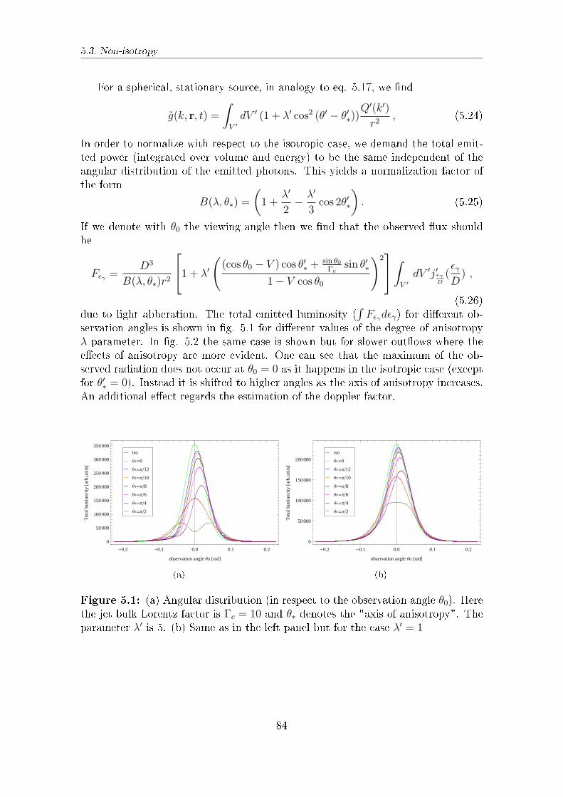
5.3. Non-isotropy
For a spherical, stationary source, in analogy to eq. 5.17, we nd
g(k, r, t) =
∫V ′
dV ′ (1 + λ′ cos2 (θ′ − θ′∗))Q′(k′)
r2, (5.24)
In order to normalize with respect to the isotropic case, we demand the total emit-ted power (integrated over volume and energy) to be the same independent of theangular distribution of the emitted photons. This yields a normalization factor ofthe form
B(λ, θ∗) =
(1 +
λ′
2− λ′
3cos 2θ′∗
). (5.25)
If we denote with θ0 the viewing angle then we nd that the observed ux shouldbe
Fϵγ =D3
B(λ, θ∗)r2
1 + λ′
((cos θ0 − V ) cos θ′∗ +
sin θ0Γc
sin θ′∗
1− V cos θ0
)2∫
V ′dV ′j′ϵγ
D(ϵγD) ,
(5.26)due to light abberation. The total emitted luminosity (
∫Fϵγdϵγ) for dierent ob-
servation angles is shown in g. 5.1 for dierent values of the degree of anisotropyλ parameter. In g. 5.2 the same case is shown but for slower outows where theeects of anisotropy are more evident. One can see that the maximum of the ob-served radiation does not occur at θ0 = 0 as it happens in the isotropic case (exceptfor θ′∗ = 0). Instead it is shifted to higher angles as the axis of anisotropy increases.An additional eect regards the estimation of the doppler factor.
-0.2 -0.1 0.0 0.1 0.2
0
50 000
100 000
150 000
200 000
250 000
300 000
350 000
observation angle Θo @radD
Tot
allu
min
ocity@a
rb.u
nitsD
Θ*=Π2
Θ*=Π4
Θ*=Π6
Θ*=Π8
Θ*=Π10
Θ*=Π12
Θ*=0
iso
(a)
-0.2 -0.1 0.0 0.1 0.2
0
50 000
100 000
150 000
200 000
observation angle Θo @radD
Tot
allu
min
ocity@a
rb.u
nitsD
Θ*=Π2
Θ*=Π4
Θ*=Π6
Θ*=Π8
Θ*=Π10
Θ*=Π12
Θ*=0
iso
(b)
Figure 5.1: (a) Angular distribution (in respect to the observation angle θ0). Herethe jet bulk Lorentz factor is Γc = 10 and θ∗ denotes the "axis of anisotropy". Theparameter λ′ is 5. (b) Same as in the left panel but for the case λ′ = 1
84
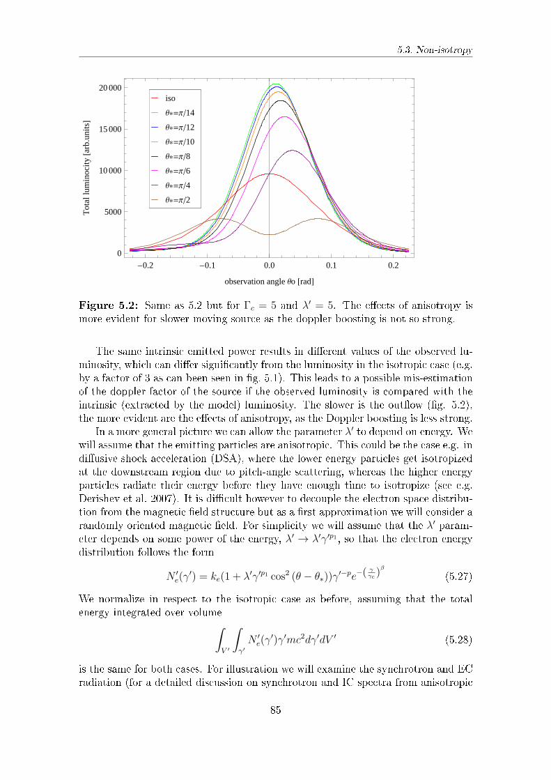
5.3. Non-isotropy
-0.2 -0.1 0.0 0.1 0.2
0
5000
10 000
15 000
20 000
observation angle Θo @radD
Tot
allu
min
ocity@a
rb.u
nitsD
Θ*=Π2
Θ*=Π4
Θ*=Π6
Θ*=Π8
Θ*=Π10
Θ*=Π12
Θ*=Π14
iso
Figure 5.2: Same as 5.2 but for Γc = 5 and λ′ = 5. The eects of anisotropy ismore evident for slower moving source as the doppler boosting is not so strong.
The same intrinsic emitted power results in dierent values of the observed lu-minosity, which can dier signicantly from the luminosity in the isotropic case (e.g.by a factor of 3 as can been seen in g. 5.1). This leads to a possible mis-estimationof the doppler factor of the source if the observed luminosity is compared with theintrinsic (extracted by the model) luminosity. The slower is the outow (g. 5.2),the more evident are the eects of anisotropy, as the Doppler boosting is less strong.
In a more general picture we can allow the parameter λ′ to depend on energy. Wewill assume that the emitting particles are anisotropic. This could be the case e.g. indiusive shock acceleration (DSA), where the lower energy particles get isotropizedat the downstream region due to pitch-angle scattering, whereas the higher energyparticles radiate their energy before they have enough time to isotropize (see e.g.Derishev et al. 2007). It is dicult however to decouple the electron space distribu-tion from the magnetic eld structure but as a rst approximation we will consider arandomly oriented magnetic eld. For simplicity we will assume that the λ′ param-eter depends on some power of the energy, λ′ → λ′γ′p1 , so that the electron energydistribution follows the form
N ′e(γ
′) = ke(1 + λ′γ′p1 cos2 (θ − θ∗))γ′−pe−(
γγc)β
(5.27)
We normalize in respect to the isotropic case as before, assuming that the totalenergy integrated over volume∫
V ′
∫γ′N ′e(γ
′)γ′mc2dγ′dV ′ (5.28)
is the same for both cases. For illustration we will examine the synchrotron and ECradiation (for a detailed discussion on synchrotron and IC spectra from anisotropic
85
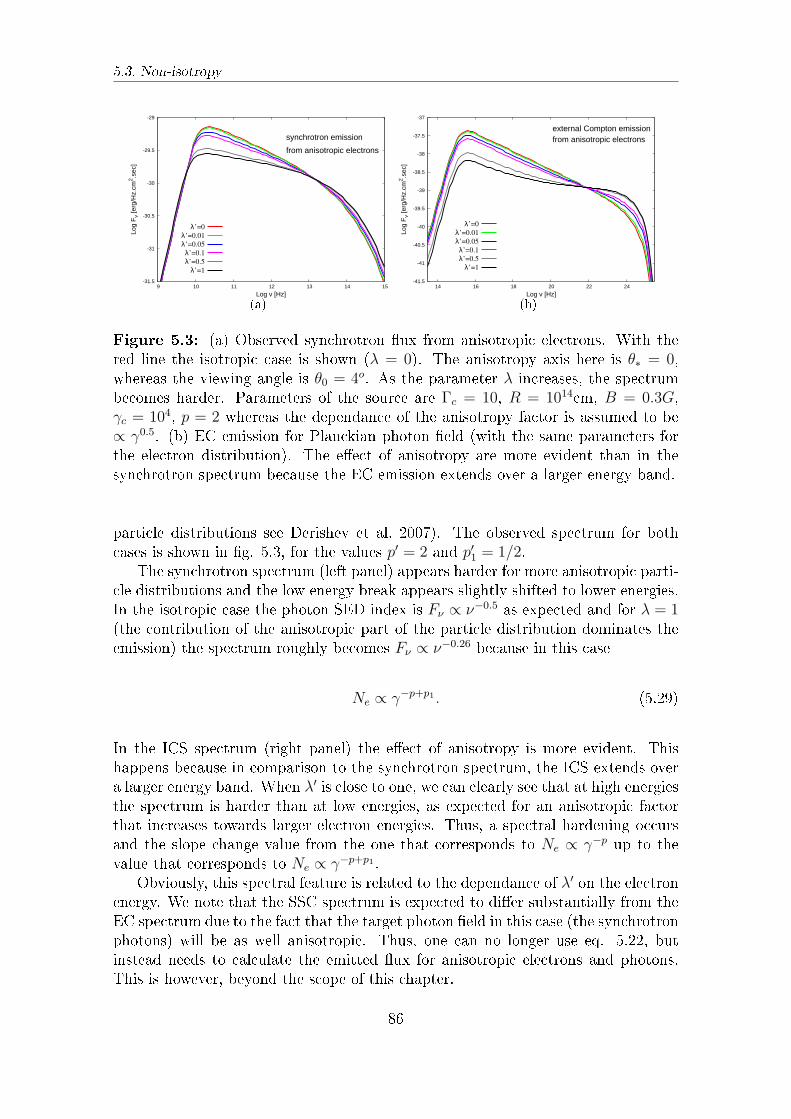
5.3. Non-isotropy
-31.5
-31
-30.5
-30
-29.5
-29
9 10 11 12 13 14 15
Log
Fv
[erg
/Hz.
cm2 .s
ec]
Log v [Hz]
synchrotron emission
from anisotropic electrons
λ’=0
λ’=0.01
λ’=0.05
λ’=0.1
λ’=0.5
λ’=1
(a)
-41.5
-41
-40.5
-40
-39.5
-39
-38.5
-38
-37.5
-37
14 16 18 20 22 24
Log
Fv
[erg
/Hz.
cm2 .s
ec]
Log v [Hz]
external Compton emissionfrom anisotropic electrons
λ’=0
λ’=0.01
λ’=0.05
λ’=0.1
λ’=0.5
λ’=1
(b)
Figure 5.3: (a) Observed synchrotron ux from anisotropic electrons. With thered line the isotropic case is shown (λ = 0). The anisotropy axis here is θ∗ = 0,whereas the viewing angle is θ0 = 4o. As the parameter λ increases, the spectrumbecomes harder. Parameters of the source are Γc = 10, R = 1014cm, B = 0.3G,γc = 104, p = 2 whereas the dependance of the anisotropy factor is assumed to be∝ γ0.5. (b) EC emission for Planckian photon eld (with the same parameters forthe electron distribution). The eect of anisotropy are more evident than in thesynchrotron spectrum because the EC emission extends over a larger energy band.
particle distributions see Derishev et al. 2007). The observed spectrum for bothcases is shown in g. 5.3, for the values p′ = 2 and p′1 = 1/2.
The synchrotron spectrum (left panel) appears harder for more anisotropic parti-cle distributions and the low energy break appears slightly shifted to lower energies.In the isotropic case the photon SED index is Fν ∝ ν−0.5 as expected and for λ = 1(the contribution of the anisotropic part of the particle distribution dominates theemission) the spectrum roughly becomes Fν ∝ ν−0.26 because in this case
Ne ∝ γ−p+p1 . (5.29)
In the ICS spectrum (right panel) the eect of anisotropy is more evident. Thishappens because in comparison to the synchrotron spectrum, the ICS extends overa larger energy band. When λ′ is close to one, we can clearly see that at high energiesthe spectrum is harder than at low energies, as expected for an anisotropic factorthat increases towards larger electron energies. Thus, a spectral hardening occursand the slope change value from the one that corresponds to Ne ∝ γ−p up to thevalue that corresponds to Ne ∝ γ−p+p1 .
Obviously, this spectral feature is related to the dependance of λ′ on the electronenergy. We note that the SSC spectrum is expected to dier substantially from theEC spectrum due to the fact that the target photon eld in this case (the synchrotronphotons) will be as well anisotropic. Thus, one can no longer use eq. 5.22, butinstead needs to calculate the emitted ux for anisotropic electrons and photons.This is however, beyond the scope of this chapter.
86
5.4. Conclusions
5.4 Conclusions
In various astrophysical objects, like AGNs, microquasars and GRBs, the ob-served ux emerges from a relativistically moving source. The Doppler boostingdue to this motion enhances substantially the emitted ux and thus the observedspectrum appears dierent than the intrinsic one. A deep understanding of theLorentz transformations that are required is important. In this chapter we haveobtained in a compact mathematically way, i.e. by solving the photon transferequation, the beaming pattern for the synchrotron, IC and SSC radiation (note thatthe formula for the synchrotron beaming pattern can be applied for any radiationmechanism for which the intrinsic photon distribution is known). Our calculationsallow for a generalization of the previously obtained results, i.e. they can account forgeneral electron distributions, non-stationary, non-homogeneous and non-isotropic.
Non-stationarity is an important characteristic especially of Blazars (but as wellas for GRBs and microquasars) because these objects are very often observed toexhibit violent changes in their ux. We have discussed that time variability aectsthe beaming pattern only if the timescale of variability is less than the dynamicaltimescale of the source. In this case however, the variations would be smoothedout and not observed in such small timescales due to casuality arguments. On theother hand, the assumption of non-isotropic particles is very well justied in variousacceleration theories, as DSA and magnetic reconnection.
We have shown that strong anisotropy modies the total luminosity, an eectthat becomes more prominent in slower (but still relativistic) outows, because themodication due to anisotropic eects competes with the eects of Doppler boosting.In respect to the isotropic case the total luminosity peaks at dierent viewing anglesand it also appears enhanced, leading to a possible mis-estimation of the sourceDoppler factor (we have normalized in respect to the total intrinsic power emitted).Under the assumption that the emitting particles are more anisotropic at higherenergies, the spectrum may appear harder. How hard the spectrum can becomeis relevant to the energy dependance that the particle distribution' s anisotropyexhibits. This eect is more evident in the EC component than in the synchrotroncomponent as it extends over a larger energy band. In any case, once anisotropiceects become evident, the slope of the emitted spectrum diers from the one thatresults from the acceleration of the particles.
87

5.4. Conclusions
88
Chapter 6
Leptonic radiation from stratied
jets
6.1 Evidence for non-homogeneous outows
As shown in the previous chapter, deviation from isotropy may lead to interestingfeatures of the observed spectrum and the total luminosity may dier signicantlyfrom the one that corresponds to the isotropic case. Another assumption that isusually made, when modeling the high energy emission of Blazars, regards the ho-mogeneity of the source. In general, the leptonic radiation is regarded to originatefrom a homogeneous (and isotropic) part of the jet, where the parameters of thebulk ow do not depend on the space coordinates. This is the case in the one-zone,homogeneous SSC model, where the parent electrons are considered to be containedin a homogeneous, spherical blob. In the EC models the same assumptions for theemitting particles are made in the majority of the cases.
However, such an approach appears adequate only to a rst approximation, sincereal jets are naturally expected to exhibit a signicant stratication. There is plentyof observational evidence that the jets' physical parameters, like the bulk velocity orthe magnetic eld, vary in space. For example, VLBI observations of the intensivelystudied Mkn 501 and Mkn 421 show a limb-brightening morphology (Giovanniniet al., 1998, 1999). A similar behavior has been observed in 3C274 and 1144+35(Giovannini et al., 2001). In the nearby radio galaxy M87 complicated structures(side-to-side oscillations, transverse expansion) are revealed by VLBI maps (Reid atal. 1989). Owen et al. (1989) have explained these structures in terms of a boundaryshear layer that dominates the dynamics of the jet. Later, radio polarization mea-surements of M87 have conrmed this complex structure. The optical jet appearsconsiderably more compact than the radio jet, and the observed knots are morecentrally concentrated (Perlman et al. 1999).
Similar morphologies have been seen in other FR I sources, such as 3C 31 (Laing,1996; Laing & Bridle, 2002) and 3C296 (Hardcastle et al. 1997), where spine-layerstructures are conrmed on kpc scales giving evidence for strong velocity shear.Even at parsec scales the radio jet of the Blazar 1055+018 exhibits a transversestructure consistent with the existence of an inner spine and a distinct boundary
89

6.1. Evidence for non-homogeneous outows
layer (Attridge et al. 1999). The polarization studies support the outcome of theradio observations as they have shown that the magnetic eld topology changeswithin the jet. The longitudinal and toroidal components become dominant indierent parts of the jet and at the boundary it does not have a transverse component(e.g. Laing et al. 2006). In the presence of a strong velocity shear, the magnetic eldtends to become parallel to the ow velocity (see e.g. Kahn, 1983; Begelman et al.,1984). This is due to the sheared ow stretching the lines of force of any magneticeld frozen into the plasma. The dominant eld direction is therefore parallel to thejet axis.
In principle the presence of brightness variations inside the jet has been con-rmed in several sources (e.g. Laing et al., 2006a,b). Apart from transverse velocitystructures, stratication along the jet has been claimed in several cases. For ex-ample, the side-to side asymmetries observed in a sample of low-luminosity FR Iradio galaxies are consistent with the hypothesis that the jet is decelerating fromrelativistic velocities close to the core to lower velocities farther away, indicatinglongitudinal velocity structures (Laing et al. 1999).
Apart from the aforementioned observational evidence for stratication, hydro-dynamical studies support as well the existence of jet stratication. Hydrodynamicalsimulations give rise to a fast spine that is surrounded by a slower layer (Aloy etal. 2000). Coupled with the magnetohydrodynamical properties of the bulk ow,synthetic synchrotron emission maps have, been investigated for a 2-component jet(an inner relativistic outow and an outer cold disk wind) in order to reproduce thelimb-brightening morphology of M87 (Gracia et al. 2009). Various MHD simulationmodels for jet formation suggest that a spine-layer structure naturally arises as theinner jet is launched by the central Black Hole via the Blandford-Znajek process,whereas the outer layer is formed from the cold disk wind (see the introduction formore details).
One should also mention that the presence of a velocity structure in the jet canresolve diculties in the unication of FR I sources and BL Lacs, if the jets ofthese sources are indeed intrinsically identical (Chiaberge et al. 2000). The dierentbeaming due to velocity dierences would then alter the observed properties of thesesources. It seems thus interesting to study in more detail the emission properties ofa jet that exhibits stratication in its bulk velocity and the magnetic eld. Addi-tionally, because the acceleration of the particles to relativistic energies depends onthese parameters, it appears promising to extend the consideration for straticationto parameters that characterize the emitting particles, such as the number densityand the maximum energy of the distribution.
The modications of the observed spectrum due to possible boundary layershas been early realized from Komissarov (1990), mainly with respect to the eectsthat the dierent relativistic beaming of the dierent parts of the jet has on theoverall spectrum. Several authors have attempted to approach open problems in theAGNs' physics and phenomenology within leptonic models assuming the radiationto originate in inhomogeneous jets. Velocity variations have been examined in boththe longitudinal and transverse direction and interesting eects of the straticationon the emitted ux have been discussed.
90
6.1. Evidence for non-homogeneous outows
Motivated by observational implications for jet deceleration Georganopoulos &Kazanas (2003) have shown that, if the jet deceleration occurs within the γ-rayemitting zone, then the particles at the base of the jet will see the photons fromthe deceleration zone boosted. This leads to an enhancement of the Compton com-ponent and allows for less extreme values of the physical parameters of the jet incomparison to the homogeneous SSC models. On the other hand, Ghisellini et al.(2005) have examined the synchrotron and Compton emission from a spine+layersystem. The interplay between the two zones through inverse Compton scatteringcan cause signicant deceleration of the jet due to Compton drag (Phinney, 1982;Sikora et al., 1996). The layer, having a smaller bulk Lorentz factor emits in a conemuch wider than the spine. Observers at large viewing angles should then see thelayer, not the spine and vice versa. Depending on whether the emission from thecore or the layer dominates the high energy component of the observed spectrum,the overall radiation from these jets may exhibit characteristics similar to the onesof BL Lac objects or FRI radio galaxies, "pairing" in this way these dierent sources(see e.g. the case of M87 in Tavecchio & Ghisellini 2008).
The transverse velocity prole that Ghisellini et al. (2005) examined is practicallya step-function. Regarding smooth transverse velocities proles, Li et al. (2004) andYang et al. (2009) have investigated the synchrotron and Compton emission from ajet with a continuous decrease of the bulk Lorentz factor from the core of the jet tothe edge. As it seems, the unication of BL Lacs and FRI may be less constrainedby the viewing angles, but rather be imprinted by velocity structures intrinsic tothe jets themselves. Furthermore, in the comoving frame, the SSC process, in thecase of a stratied jet, has properties similar to the EC model (Li & Wang 2004).
Once a velocity structure exists in the jet, additional particle acceleration is ex-pected to occur in the shear ow (see e.g. Rieger & Duy 2004). As the particlesscatter of the magnetic eld inhomogeneities, they gain energy traveling through theshear. This stochastic process can be ecient enough to lead to the formation ofrelativistic particle distributions. The diusive shock acceleration process seems tobe a plausible mechanism for the origin of the non-thermal power-law distributionsin the case of relativistic parsec scale AGN jets. In large-scale jets however, shear ac-celeration might represent an attractive mechanism for boosting of particles at highenergies (Rieger et al. 2007). In any case, even in small scale jets, it is possible thatstochastic processes operate at least complementary to the DSA (re-acceleration).
Stawarz & Ostrowski (2002) examined the expected radiated spectra of suchdistributions that can be generated at the boundary shear layers of large scales jets,showing that the emission of these electrons can substantially contribute to the jetradiative output and create observational signatures characteristic of the shear ac-celeration. Aloy & Mimica (2008) further investigate more complex velocity prolesin order to show observable dierences with respect to conventional monotonic andsmooth boundary layers.
Obviously, studying the emission properties of a jet that exhibits straticationseems not only highly motivated by observations, but it also appears promising forapproaching unresolved puzzles in AGNs' physics and phenomenology. Deviationfrom the standard, homogeneous models requires careful investigation of the eects
91
6.2. Relativistic jet with stratication at the transverse direction
that processes like Compton scattering, relativistic beaming or possible shear accel-eration may have on the observed spectrum.
In this chapter we examine the synchrotron radiation from a jet that exhibitsstratication in the bulk Lorentz factor, the magnetic eld, but also in the numberdensity and the maximum energy of the electron distribution. The reasoning forthe latter two varying parameters regards the fact that the characteristics of theelectron population are bounded to the bulk ow physical parameters through theacceleration process. We consider transverse velocity and magnetic eld proles andwe assume that the dominating cooling process is synchrotron radiation.
6.2 Relativistic jet with stratication at the trans-
verse direction
Let us consider an axisymmetric, irrotational, relativistic jet emerging from thecentral engine of the AGN. In cylindrical coordinates, each point of the jet is char-acterized by the position vector r = (ϖ,ϕ, z), where z is the (longitudinal) distancefrom the core, ϖ is the cylindrical (transverse) radius and ϕ the azimuthal angle(see the sketch in g. 6.1). The outow is moving in the z-direction. We assumethat the jet is suciently collimated at distance z0 ∼ 1016cm (sub-parsec scale jet),which will be referred to as the base of the jet. This value for z0 is consistent withMHD studies and moreover it is far away enough from the disk where intense photoneld may exist and cool down the particle distribution very rapidly. At z0 the outerradius is of the order of ϖ(z = z0) ≡ R0 ∼ z0/10. Up to a distance z1 we approxi-mate the shape of the jet with a cylinder, i.e. the outer radius varies very slowly inrespect to z, R(z) ∼ R0 ≈ constant. For z > z1 the jet may start to expand in theϖ direction, introducing adiabatic losses that make the particles inecient emitters.
We consider a scheme where relativistic electrons are injected at the base of thejet, e.g. by 1st order Fermi acceleration at a standing shock. The presence/creationof standing shocks inside the jet has been suggested before (for instance, recollima-tion shocks in an initially over-pressurized outow (Gomez et al., 1995; Perucho &Martí, 2007). The radiation of the particles that are accelerated in such shocks maydominate the observed spectrum (e.g. Mandal & Chakrabarti, 2008; Becker et al.,2008).
Let K ′ be the comoving ow frame and K the observer' s frame. The energydistribution of the injected electrons at the base of the jet is assumed to be a power-law with varying (with respect to ϖ coordinate) number density and maximumcuto
n′0ϖ(γ
′0) = k′
0ϖγ′−s0 Θ(γ′
0 − γ′0,min)Θ(γ′
0,max − γ′0). (6.1)
From now on we will use the notation Xzϖ = X(z,ϖ) for the parameter thatdepend on both spatial coordinates, ϖ and z. Thus X0ϖ symbolizes the value of theparameter X at (z = 0, ϖ). An exception holds for the electrons Lorentz factors,with gamma′0 to imply that the particles are the base of the edge at any radius andγ′ to refer to an arbitrary point (ϖ, z) of the outow. The parameters that dependonly on the polar radius will be simply denoted as X(ϖ).
92
6.2. Relativistic jet with stratication at the transverse direction
The bulk velocity and Lorentz factor of the ow exhibit dependance on thecylindrical radius
β = β(ϖ), Γ = Γ(ϖ) =1√
1− β(ϖ)2, (6.2)
and thus the Doppler factor at each point (z,ϖ) is
D(ϖ) =1
Γ(ϖ)(1− β(ϖ)cosθ0), (6.3)
implying dierent beaming for each point of the jet. As we will consider decreasingvelocity proles from the center to the edge, the inner layers of the jet will radiate ina smaller cone than the outer layers. We furthermore assume that the magnetic elddepends as well on the ϖ coordinate, B = B(ϖ). For simplicity, we consider thatthe dominant cooling process is synchrotron radiation. The particles loose energyas they travel along the jet according to
dγ′
dz′=
dγ′
dt′dt′
dz′= −4
3
σT c
mc2U ′B(ϖ)γ′2 dt
′
dz′. (6.4)
It holds that dz′ = cβ(ϖ)dt′ and due to Lorentz transformations, dz = Γ(ϖ)dz′, wend
dγ′
dz=
dγ′
Γ(ϖ)dz′=
1
cβ(ϖ)Γ(ϖ)
dγ′
dt′. (6.5)
In principle, all the parameters are expressed for convenience in the comoving frame,apart from the spatial coordinates. Practically, z corresponds to the time neededfor an electron to travel from the base of the jet up to the point z. Note that thisis not the time coordinate. The outow is stationary and thus the radiation thatan observer receives is independent on whether the timescales of observation aresmaller or larger than the light crossing time of the jet.
By expressing all spatial coordinates at the observer' s frame K we reach to theformula
dγ′
dz= −C ′(r)γ′ 2, C ′(ϖ) =
4
3
σTU′B(ϖ)
mc21
Γ(ϖ)β(ϖ). (6.6)
The solution of equation 6.6 results in the energy evolution of monoenergetic elec-trons with initial Lorentz factor γ′
0
γ′ =γ′0
C ′(ϖ)(z − z0)γ′0 + 1
. (6.7)
Determining the electron distribution at any point (z,ϖ) of the jet can be performedin two equivalent ways. Either through the electron number conservation or by solv-ing the kinetic equation after replacing (t → z). For a stationary, incompressible andirrotational ow (without shear or vorticity) the volume element is constant alongthe ow. Thus, from the conservation of the total number of particles (integratedover energies) it follows that
n′0ϖ(γ
′0)dγ
′0 = n′
zϖ(γ′)dγ′. (6.8)
93
6.2. Relativistic jet with stratication at the transverse direction
We can easily calculate dγ′0/dγ
′ = (1 − γ′C ′(ϖ)(z − z0))−2, which, in combination
with equations (6.1) and (6.6), leads to the electron's energy distribution at anarbitrary point (z,ϖ) of the jet
n′zϖ(γ
′) = k′0ϖ
γ′−s
[1− γ′C ′(ϖ)(z − z0)]2−sΘ(γ′ − γ′
max)Θ(γ′min − γ′), (6.9)
where the minimum and maximum cuto energies are given by
γ′min =
γ′0,min
C(ϖ)(z − z0)γ′0,min + 1
, γ′z,min =
γ′0,max
C(ϖ)(z − z0)γ′0,max + 1
. (6.10)
The local electron energy distribution preserves almost the same shape of the in-jected one, while the minimum and maximum cuto decrease as shown in gure(6.2). The same result can alternatively be reached using the electrons' kineticequation for synchrotron losses
ϑn′zϖ(γ
′)
ϑt′=
ϑ
ϑγ′ (γ′n′zϖ(γ
′)) , (6.11)
with the initial conditions imposed by equation (6.1). Changing the integrationvariable to z = Γ(ϖ)β(ϖ)ct′, we can write
ϑn′zϖ(γ
′)
ϑz= C ′(ϖ)
ϑ
ϑγ′
(γ′2n′
zϖ(γ′)). (6.12)
The above equation has the solution of equation (6.9) (see Kardashev 1962) andallows to add more terms for possible energy losses or acceleration of the electrons.
So there is a characteristic length scale at which the electrons have radiated awayall o their energy and completely cooled down. We may dene this distance as
zcool = z0 +1
γ′0C
′(ϖ)+
1
C ′(ϖ)(6.13)
in which the third term dominates (for γ′0 ≫ 1), implying practically that this
cooling length scale does not strongly depend on the initial energy of the particles,mainly because of the way electrons cool down as shown in g. (6.2). Two distinctcases can be examined. Either the electrons lose all their energy before reaching the"top" of the jet, at a xed distance z1 imposed e.g. by the domination of adiabaticlosses after a certain distance from the jet base, or they escape from the radiatingzone before they completely cool down due to synchrotron losses.
94
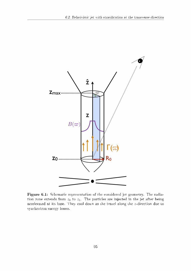
6.2. Relativistic jet with stratication at the transverse direction
z
z0
zmax
z
R0
Φ
Γ( )
B()
Figure 6.1: Schematic representation of the considered jet geometry. The radia-tion zone extends from z0 to z1. The particles are injected in the jet after beingaccelerated at its base. They cool down as the travel along the z-direction due tosynchrotron energy losses.
95
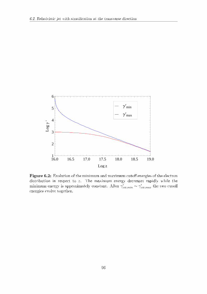
6.2. Relativistic jet with stratication at the transverse direction
16.0 16.5 17.0 17.5 18.0 18.5 19.01
2
3
4
5
6
Log z
LogΓ
'
Γ'max
Γ'min
Figure 6.2: Evolution of the minimum and maximum cuto energies of the electrondistribution in respect to z. The maximum energy decreases rapidly while theminimum energy is approximately constant. After γ′
zϖ,min ∼ γ′zϖ,max the two cuto
energies evolve together.
96
6.3. Properties of the layers
6.3 Properties of the layers
The reason that we have not yet specied the ϖ-dependance for the parametersof the jet and the particle distribution concerns the fact that integration over thez-coordinate is not aected by the variations along the cylindrical coordinate. Thehidden assumption is that the particles' mean free path is smaller than the scaleat which the velocity changes signicantly. Thus, one may determine the particledistribution, as well as the synchrotron emission, in each layer. This can be illus-trating for the multiple luminosity proles from dierent velocity and magnetic eldstructures.
6.3.1 Electron distribution integrated over the longitudinal
direction
With the local electron energy distribution of equation (6.9) at hand, the z-integrated energy distribution reads
n′ϖ(γ
′) =
∫ z1
z0
n′zϖ(γ
′)dz. (6.14)
From the properties of the heaviside step-function yields that
Θ(γ′ − γ′min) = Θ (z − zmin(γ
′)) , Θ(γ′max − γ′) = Θ (zmax(γ
′)− z) , (6.15)
where
zmin(γ′) = zo +
1
C ′(ϖ)
(1
γ′ −1
γ′0,min
), zmax(γ
′) = zo +1
C ′(ϖ)
(1
γ′ −1
γ′0,max
).
(6.16)Due to the above limitations, the integration limits become
n′ϖ(γ
′) =
∫ min[z1,zmax(γ′)]
max[z0,zmin(γ′)]
k′0ϖγ
′−s
[1− γ′C ′(ϖ)(z − z0)]2−sdz. (6.17)
The comparison of the various length scale elements entering the limits of integrationwill reveal the dierent branches of the solution. One can see e.g. that z1 < zmax(γ
′),when γ′ < γ′
1,max. The Lorentz factor γ′1,max corresponds to the energy that an
electron should have when it reaches the top of the jet, if it's initial energy is at thehigh energy cuto γ′
0,max
γ′1,max ≡
γ′0,max
1 + C ′(ϖ)(z1 − z0)γ′0max
. (6.18)
The value of γ′1,min for the injected low cuto energy is correspondingly
γ′1,min ≡
γ′0,min
1 + C ′(ϖ)(z1 − z0)γ′0min
. (6.19)
Investigating all the limits of the integral and assuring that none of them overlapreveals two cases for the electron distribution depending on the maximum lengthscale and the injected low energy cuto value.
97
6.3. Properties of the layers
• γ′1,max > γ′
0,min: The electrons with injected energy at the maximum cutohave not cooled below γ′
0,min at the top of the jet.• γ′
1,max < γ′0,min: The electrons with injected energy at the maximum cuto
have traveled a long enough distance to reduce their energy below γ′0,min at
the top of the jet.In the former case, the solution becomes
n′ϖ(γ
′) = Λ(ϖ)
γ′−s−1
[(1− γ′C ′(ϖ)(z1 − z0))
s−1 −(
γ′
γ′0,min
)s−1], γ′
1,min < γ′ < γ′0,min
γ′−s−1[(1− γ′C(ϖ)(z1 − z0))
s−1 − 1], γ′
0,min < γ′ < γ′1,max
γ′−s−1
[(γ′
γ0,max
)s−1
− 1
], γ′
1,max < γ′ < γ′0,max
(6.20)where
Λ(ϖ) =k0ϖ
C ′(ϖ)(1− s). (6.21)
The last branch of the expression represent the cooled distribution, for which thepower-law index becomes steeper by 1. The particles with energy below γ′
1,max havenot cooled, thus the distribution is proportional to γ′−s. The rst branch correspondsto a cuto practically at γ′
0,min. The injected electrons with energy γ′0,min have not
reduced signicantly their energy, even when reaching the top of the jet, and thusγ′1,min ∼ γ′
0,min. For illustration see g. 6.3.When the opposite situation occurs, γ′
1,max < γ′0,min, the solution takes the form
n′ϖ(γ
′) = λ(ϖ)
γ′−s−1
[(1− γ′C ′(ϖ)(z1 − z0))
s−1 −(
γ′
γ′0,min
)s−1], γ′
1,min < γ′ < γ′1,max
γ′−2[γ′1−s0,max − γ′1−s
0,max
], γ′
1,max < γ′ < γ′0,min
γ′−s−1
[(γ′
γ0,max
)s−1
− 1
], γ′
0,min < γ′ < γ′0,max
(6.22)Here all the particles completely cool down and thus the distribution exhibits twopower-law indexes, n′
ϖ(γ′) ∝ γ′−2 at high energies and n′
ϖ(γ′) ∝ γ′−s−1 at energies
below γ′0,min. The rst branch shows, as before, a cuto. For constant physical
parameters (no stratication) the jet geometry gives rise to particle distributionsequivalent with the ones emerging from a spherical blob. The value of the timeneeded for the particles to escape the blob would then allow to distinguish betweenthe two cases discussed above. Actually the condition γ′
0min ∼ γ′1,max demonstrates
what the horizontal size of the jet should be, in order to result in the rst or secondsolution. If z < z∗1 , the size of the jet is not large enough to allow the injectedelectrons at the maximum cuto to cool down to γ′
0,min so that we take the rst
98
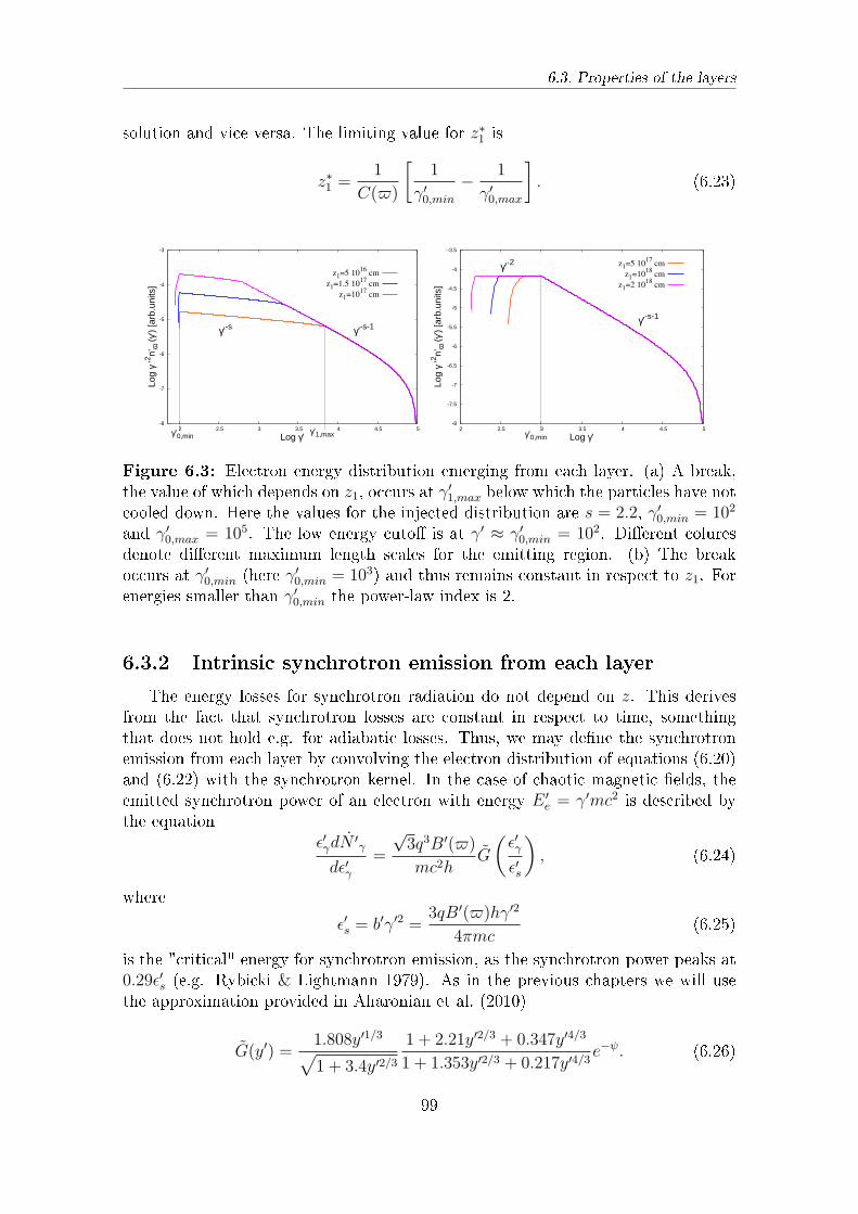
6.3. Properties of the layers
solution and vice versa. The limiting value for z∗1 is
z∗1 =1
C(ϖ)
[1
γ′0,min
− 1
γ′0,max
]. (6.23)
-8
-7
-6
-5
-4
-3
2 2.5 3 3.5 4 4.5 5
Log
γ ’2 n’
ϖ (γ
’) [a
rb.u
nits
]
Log γ’
γ’-s-1γ’-s
γ’1,maxγ’0,min
z1=5 10
16 cm
z1=1.5 10
17 cm
z1=10
17 cm
-8
-7.5
-7
-6.5
-6
-5.5
-5
-4.5
-4
-3.5
2 2.5 3 3.5 4 4.5 5
Log
γ ’2 n’
ϖ (γ
’) [a
rb.u
nits
]Log γ’
γ’-s-1
γ’-2
γ’0,min
z1=5 10
17 cm
z1=10
18 cm
z1=2 10
18 cm
Figure 6.3: Electron energy distribution emerging from each layer. (a) A break,the value of which depends on z1, occurs at γ′
1,max below which the particles have notcooled down. Here the values for the injected distribution are s = 2.2, γ′
0,min = 102
and γ′0,max = 105. The low energy cuto is at γ′ ≈ γ′
0,min = 102. Dierent coluresdenote dierent maximum length scales for the emitting region. (b) The breakoccurs at γ′
0,min (here γ′0,min = 103) and thus remains constant in respect to z1. For
energies smaller than γ′0,min the power-law index is 2.
6.3.2 Intrinsic synchrotron emission from each layer
The energy losses for synchrotron radiation do not depend on z. This derivesfrom the fact that synchrotron losses are constant in respect to time, somethingthat does not hold e.g. for adiabatic losses. Thus, we may dene the synchrotronemission from each layer by convolving the electron distribution of equations (6.20)and (6.22) with the synchrotron kernel. In the case of chaotic magnetic elds, theemitted synchrotron power of an electron with energy E ′
e = γ′mc2 is described bythe equation
ϵ′γdN′γ
dϵ′γ=
√3q3B′(ϖ)
mc2hG
(ϵ′γϵ′s
), (6.24)
where
ϵ′s = b′γ′2 =3qB′(ϖ)hγ′2
4πmc(6.25)
is the "critical" energy for synchrotron emission, as the synchrotron power peaks at0.29ϵ′s (e.g. Rybicki & Lightmann 1979). As in the previous chapters we will usethe approximation provided in Aharonian et al. (2010)
G(y′) =1.808y′1/3√1 + 3.4y′2/3
1 + 2.21y′2/3 + 0.347y′4/3
1 + 1.353y′2/3 + 0.217y′4/3e−ψ. (6.26)
99
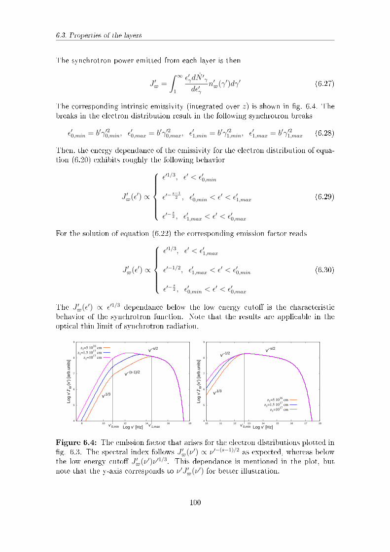
6.3. Properties of the layers
The synchrotron power emitted from each layer is then
J ′ϖ =
∫ ∞
1
ϵ′γdN′γ
dϵ′γn′ϖ(γ
′)dγ′ (6.27)
The corresponding intrinsic emissivity (integrated over z) is shown in g. 6.4. Thebreaks in the electron distribution result in the following synchrotron breaks
ϵ′0,min = b′γ′20,min, ϵ′0,max = b′γ′2
0,max, ϵ′1,min = b′γ′21,min, ϵ′1,max = b′γ′2
1,max (6.28)
Then, the energy dependance of the emissivity for the electron distribution of equa-tion (6.20) exhibits roughly the following behavior
J ′ϖ(ϵ
′) ∝
ϵ′1/3, ϵ′ < ϵ′0,min
ϵ′−s−12 , ϵ′0,min < ϵ′ < ϵ′1,max
ϵ′−s2 , ϵ′1,max < ϵ′ < ϵ′0,max
(6.29)
For the solution of equation (6.22) the corresponding emission factor reads
J ′ϖ(ϵ
′) ∝
ϵ′1/3, ϵ′ < ϵ′1,max
ϵ′−1/2, ϵ′1,max < ϵ′ < ϵ′0,min
ϵ′−s2 , ϵ′0,min < ϵ′ < ϵ′0,max
(6.30)
The J ′ϖ(ϵ
′) ∝ ϵ′1/3 dependance below the low energy cuto is the characteristicbehavior of the synchrotron function. Note that the results are applicable in theoptical thin limit of synchrotron radiation.
4
5
6
7
8
9
8 10 12 14 16 18
Log
v’J’
ϖ (v
’) [a
rb.u
nits
]
Log v’ [Hz]
v’-s/2
v’-(s-1)/2
v’1/3
v’1,maxv’0,min
z1=5 10
16 cm
z1=1.5 10
17 cm
z1=10
17 cm
4
5
6
7
8
9
10 11 12 13 14 15 16 17 18
Log
v’J’
ϖ (v
’) [a
rb.u
nits
]
Log v’ [Hz]
v’-s/2
v’-1/2
v’1/3
v’0,min
z1=5 10
16 cm
z1=1.5 10
17 cm
z1=10
17 cm
Figure 6.4: The emission factor that arises for the electron distributions plotted ing. 6.3. The spectral index follows J ′
ϖ(ν′) ∝ ν ′−(s−1)/2 as expected, whereas below
the low energy cuto J ′ϖ(ν
′)ν ′1/3. This dependance is mentioned in the plot, butnote that the y-axis corresponds to ν ′J ′
ϖ(ν′) for better illustration.
100
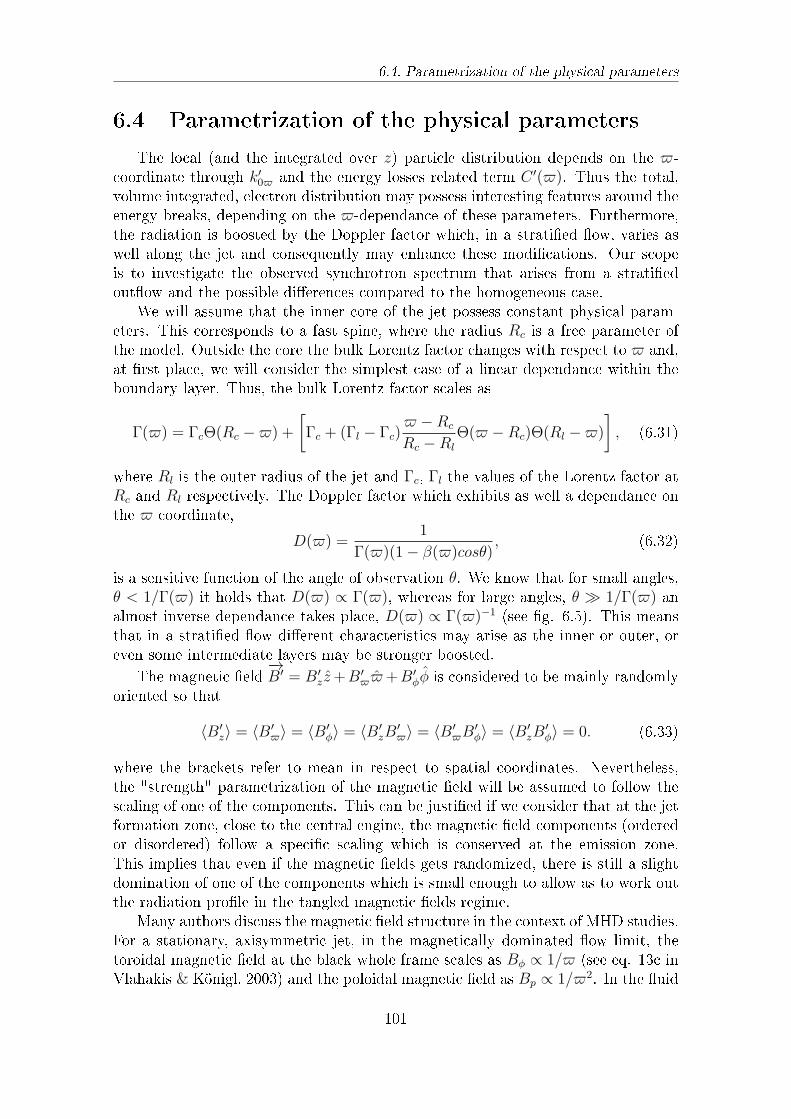
6.4. Parametrization of the physical parameters
6.4 Parametrization of the physical parameters
The local (and the integrated over z) particle distribution depends on the ϖ-coordinate through k′
0ϖ and the energy losses related term C ′(ϖ). Thus the total,volume integrated, electron distribution may possess interesting features around theenergy breaks, depending on the ϖ-dependance of these parameters. Furthermore,the radiation is boosted by the Doppler factor which, in a stratied ow, varies aswell along the jet and consequently may enhance these modications. Our scopeis to investigate the observed synchrotron spectrum that arises from a stratiedoutow and the possible dierences compared to the homogeneous case.
We will assume that the inner core of the jet possess constant physical param-eters. This corresponds to a fast spine, where the radius Rc is a free parameter ofthe model. Outside the core the bulk Lorentz factor changes with respect to ϖ and,at rst place, we will consider the simplest case of a linear dependance within theboundary layer. Thus, the bulk Lorentz factor scales as
Γ(ϖ) = ΓcΘ(Rc −ϖ) +
[Γc + (Γl − Γc)
ϖ −Rc
Rc −Rl
Θ(ϖ −Rc)Θ(Rl −ϖ)
], (6.31)
where Rl is the outer radius of the jet and Γc, Γl the values of the Lorentz factor atRc and Rl respectively. The Doppler factor which exhibits as well a dependance onthe ϖ coordinate,
D(ϖ) =1
Γ(ϖ)(1− β(ϖ)cosθ), (6.32)
is a sensitive function of the angle of observation θ. We know that for small angles,θ < 1/Γ(ϖ) it holds that D(ϖ) ∝ Γ(ϖ), whereas for large angles, θ ≫ 1/Γ(ϖ) analmost inverse dependance takes place, D(ϖ) ∝ Γ(ϖ)−1 (see g. 6.5). This meansthat in a stratied ow dierent characteristics may arise as the inner or outer, oreven some intermediate layers may be stronger boosted.
The magnetic eld−→B′ = B′
z z+B′ϖϖ+B′
ϕϕ is considered to be mainly randomlyoriented so that
⟨B′z⟩ = ⟨B′
ϖ⟩ = ⟨B′ϕ⟩ = ⟨B′
zB′ϖ⟩ = ⟨B′
ϖB′ϕ⟩ = ⟨B′
zB′ϕ⟩ = 0. (6.33)
where the brackets refer to mean in respect to spatial coordinates. Nevertheless,the "strength" parametrization of the magnetic eld will be assumed to follow thescaling of one of the components. This can be justied if we consider that at the jetformation zone, close to the central engine, the magnetic eld components (orderedor disordered) follow a specic scaling which is conserved at the emission zone.This implies that even if the magnetic elds gets randomized, there is still a slightdomination of one of the components which is small enough to allow as to work outthe radiation prole in the tangled magnetic elds regime.
Many authors discuss the magnetic eld structure in the context of MHD studies.For a stationary, axisymmetric jet, in the magnetically dominated ow limit, thetoroidal magnetic eld at the black whole frame scales as Bϕ ∝ 1/ϖ (see eq. 13c inVlahakis & Königl, 2003) and the poloidal magnetic eld as Bp ∝ 1/ϖ2. In the uid
101
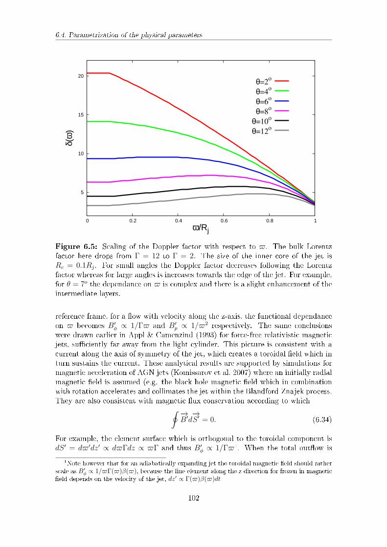
6.4. Parametrization of the physical parameters
5
10
15
20
0 0.2 0.4 0.6 0.8 1
δ(ϖ
)
ϖ/Rj
θ=2o
θ=4o
θ=6o
θ=8o
θ=10o
θ=12o
Figure 6.5: Scaling of the Doppler factor with respect to ϖ. The bulk Lorentzfactor here drops from Γ = 12 to Γ = 2. The size of the inner core of the jet isRc = 0.1Rj. For small angles the Doppler factor decreases following the Lorentzfactor whereas for large angles is increases towards the edge of the jet. For example,for θ = 7o the dependance on ϖ is complex and there is a slight enhancement of theintermediate layers.
reference frame, for a ow with velocity along the z-axis, the functional dependanceon ϖ becomes B′
ϕ ∝ 1/Γϖ and B′p ∝ 1/ϖ2 respectively. The same conclusions
were drawn earlier in Appl & Camenzind (1993) for force-free relativistic magneticjets, suciently far away from the light cylinder. This picture is consistent with acurrent along the axis of symmetry of the jet, which creates a toroidal eld which inturn sustains the current. These analytical results are supported by simulations formagnetic acceleration of AGN jets (Komissarov et al. 2007) where an initially radialmagnetic eld is assumed (e.g. the black hole magnetic eld which in combinationwith rotation accelerates and collimates the jet within the Blandford-Znajek process.They are also consistent with magnetic ux conservation according to which∮ −→
B′d−→S ′ = 0. (6.34)
For example, the element surface which is orthogonal to the toroidal component isdS ′ = dϖ′dz′ ∝ dϖΓdz ∝ ϖΓ and thus B′
ϕ ∝ 1/Γϖ1. When the total outow is
1Note however that for an adiabatically expanding jet the toroidal magnetic eld should ratherscale as B′
ϕ ∝ 1/ϖΓ(ϖ)β(ϖ), because the line element along the z direction for frozen in magneticeld depends on the velocity of the jet, dz′ ∝ Γ(ϖ)β(ϖ)dt
102
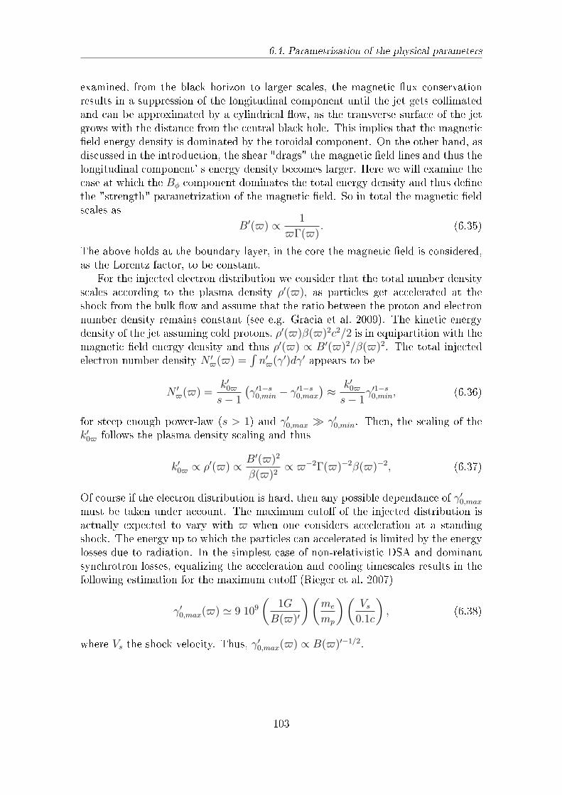
6.4. Parametrization of the physical parameters
examined, from the black horizon to larger scales, the magnetic ux conservationresults in a suppression of the longitudinal component until the jet gets collimatedand can be approximated by a cylindrical ow, as the transverse surface of the jetgrows with the distance from the central black hole. This implies that the magneticeld energy density is dominated by the toroidal component. On the other hand, asdiscussed in the introduction, the shear "drags" the magnetic eld lines and thus thelongitudinal component' s energy density becomes larger. Here we will examine thecase at which the Bϕ component dominates the total energy density and thus denethe "strength" parametrization of the magnetic eld. So in total the magnetic eldscales as
B′(ϖ) ∝ 1
ϖΓ(ϖ). (6.35)
The above holds at the boundary layer, in the core the magnetic eld is considered,as the Lorentz factor, to be constant.
For the injected electron distribution we consider that the total number densityscales according to the plasma density ρ′(ϖ), as particles get accelerated at theshock from the bulk ow and assume that the ratio between the proton and electronnumber density remains constant (see e.g. Gracia et al. 2009). The kinetic energydensity of the jet assuming cold protons, ρ′(ϖ)β(ϖ)2c2/2 is in equipartition with themagnetic eld energy density and thus ρ′(ϖ) ∝ B′(ϖ)2/β(ϖ)2. The total injectedelectron number density N ′
ϖ(ϖ) =∫n′ϖ(γ
′)dγ′ appears to be
N ′ϖ(ϖ) =
k′0ϖ
s− 1
(γ′1−s0,min − γ′1−s
0,max
)≈ k′
0ϖ
s− 1γ′1−s0,min, (6.36)
for steep enough power-law (s > 1) and γ′0,max ≫ γ′
0,min. Then, the scaling of thek′0ϖ follows the plasma density scaling and thus
k′0ϖ ∝ ρ′(ϖ) ∝ B′(ϖ)2
β(ϖ)2∝ ϖ−2Γ(ϖ)−2β(ϖ)−2, (6.37)
Of course if the electron distribution is hard, then any possible dependance of γ′0,max
must be taken under account. The maximum cuto of the injected distribution isactually expected to vary with ϖ when one considers acceleration at a standingshock. The energy up to which the particles can accelerated is limited by the energylosses due to radiation. In the simplest case of non-relativistic DSA and dominantsynchrotron losses, equalizing the acceleration and cooling timescales results in thefollowing estimation for the maximum cuto (Rieger et al. 2007)
γ′0,max(ϖ) ≃ 9 109
(1G
B(ϖ)′
)(me
mp
)(Vs0.1c
), (6.38)
where Vs the shock velocity. Thus, γ′0,max(ϖ) ∝ B(ϖ)′−1/2.
103
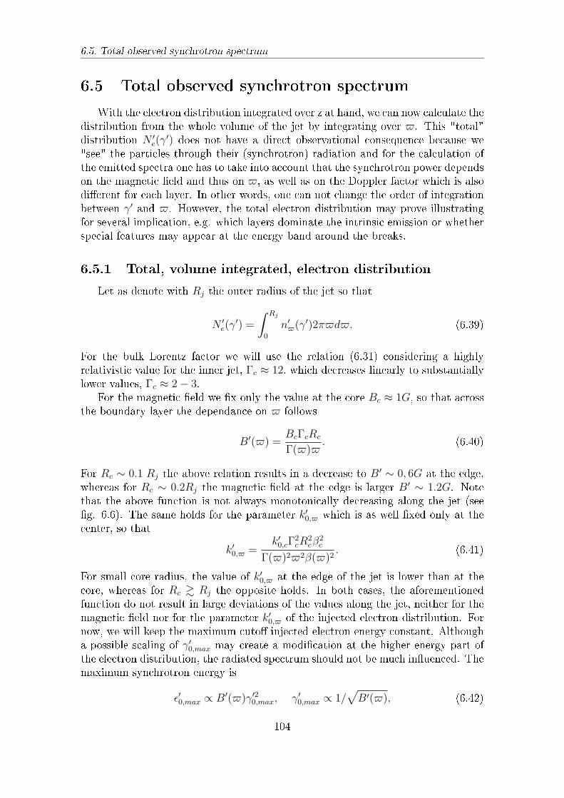
6.5. Total observed synchrotron spectrum
6.5 Total observed synchrotron spectrum
With the electron distribution integrated over z at hand, we can now calculate thedistribution from the whole volume of the jet by integrating over ϖ. This "total"distribution N ′
e(γ′) does not have a direct observational consequence because we
"see" the particles through their (synchrotron) radiation and for the calculation ofthe emitted spectra one has to take into account that the synchrotron power dependson the magnetic eld and thus on ϖ, as well as on the Doppler factor which is alsodierent for each layer. In other words, one can not change the order of integrationbetween γ′ and ϖ. However, the total electron distribution may prove illustratingfor several implication, e.g. which layers dominate the intrinsic emission or whetherspecial features may appear at the energy band around the breaks.
6.5.1 Total, volume integrated, electron distribution
Let as denote with Rj the outer radius of the jet so that
N ′e(γ
′) =
∫ Rj
0
n′ϖ(γ
′)2πϖdϖ. (6.39)
For the bulk Lorentz factor we will use the relation (6.31) considering a highlyrelativistic value for the inner jet, Γc ≈ 12, which decreases linearly to substantiallylower values, Γc ≈ 2− 3.
For the magnetic eld we x only the value at the core Bc ≈ 1G, so that acrossthe boundary layer the dependance on ϖ follows
B′(ϖ) =BcΓcRc
Γ(ϖ)ϖ. (6.40)
For Rc ∼ 0.1 Rj the above relation results in a decrease to B′ ∼ 0, 6G at the edge,whereas for Rc ∼ 0.2Rj the magnetic eld at the edge is larger B′ ∼ 1.2G. Notethat the above function is not always monotonically decreasing along the jet (seeg. 6.6). The same holds for the parameter k′
0,ϖ which is as well xed only at thecenter, so that
k′0,ϖ =
k′0,cΓ
2cR
2cβ
2c
Γ(ϖ)2ϖ2β(ϖ)2. (6.41)
For small core radius, the value of k′0,ϖ at the edge of the jet is lower than at the
core, whereas for Rc & Rj the opposite holds. In both cases, the aforementionedfunction do not result in large deviations of the values along the jet, neither for themagnetic eld nor for the parameter k′
0,ϖ of the injected electron distribution. Fornow, we will keep the maximum cuto injected electron energy constant. Althougha possible scaling of γ′
0,max may create a modication at the higher energy part ofthe electron distribution, the radiated spectrum should not be much inuenced. Themaximum synchrotron energy is
ϵ′0,max ∝ B′(ϖ)γ′20,max, γ′
0,max ∝ 1/√B′(ϖ), (6.42)
104
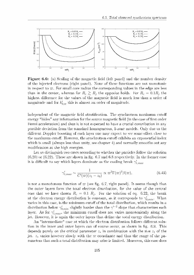
6.5. Total observed synchrotron spectrum
0
0.2
0.4
0.6
0.8
1
1.2
0 0.2 0.4 0.6 0.8 1
B’(ϖ
) [G
auss
]
ϖ/Rj
Rc = 0.05 RjRc = 0.1 RjRc = 0.2 Rj
18
18.5
19
19.5
20
20.5
0 0.2 0.4 0.6 0.8 1
k’0,
ϖ [c
m-3
]
ϖ/Rj
Rc = 0.05 RjRc = 0.1 RjRc = 0.2 Rj
Figure 6.6: (a) Scaling of the magnetic eld (left panel) and the number densityof the injected electrons (right panel). None of these functions are not monotonicin respect to ϖ. For small core radius the corresponding values in the edge are lessthan in the center, whereas for Rc & Rj the opposite holds. For Rc = 0.1Rj thehighest dierence for the values of the magnetic eld is much less than a order ofmagnitude and for k′
0,ϖ this is almost an order of magnitude.
independent of the magnetic eld stratication. The synchrotron maximum cutoenergy "hides" any information for the source magnetic eld (in the case of rst orderFermi acceleration) and thus it is not expected to have a crucial contribution in anypossible deviation from the standard homogeneous, 1-zone models. Only due to thedierent Doppler boosting of each layer one may expect to see some eect close tothe maximum cuto. However, the synchrotron cuto exhibits an exponential indexwhich is small (always less than unity, see chapter 4) and normally smooths out anymodication at the high energies.
Let us distinguish two cases according to whether the particles follow the solution(6.20) or (6.22). These are shown in g. 6.7 and 6.8 respectively. In the former caseit is dicult to say which layers dominate as the cooling break γ′
1,max
γ′1,max ∼
1
C ′(ϖ)(z1 − z0)∝ ϖ2Γ(ϖ)3β(ϖ), (6.43)
is not a monotonous function of ϖ (see g. 6.7, right panel). It seems though thatthe outer layers form the total electron distribution, for the value of the centralcore that we have chosen Rc = 0.1 Rj. For the solution of eq. 6.22, the breakat the electron energy distribution is constant, as it corresponds to γ′
0,min. Whatvaries in this case, is the minimum cuto of the total distribution, which results in adistribution below γ′
0,min slightly harder than the γ′−2 slope that characterizes eachlayer. As for γ′
1,max, the minimum cuto does not varies monotonically along thejet. However, it is again the outer layers that dene the total energy distribution.
An "intermediate" case at which the electron distribution follows dierent solu-tion in the inner and outer layers can of course occur, as shown in g. 6.9. Thisdepends purely on the critical parameter z∗ in combination with the size z1 of thejet. z∗ varies however slowly with the ϖ coordinate and thus the range of the pa-rameters that such a total distribution may arise is limited. Moreover, this case does
105
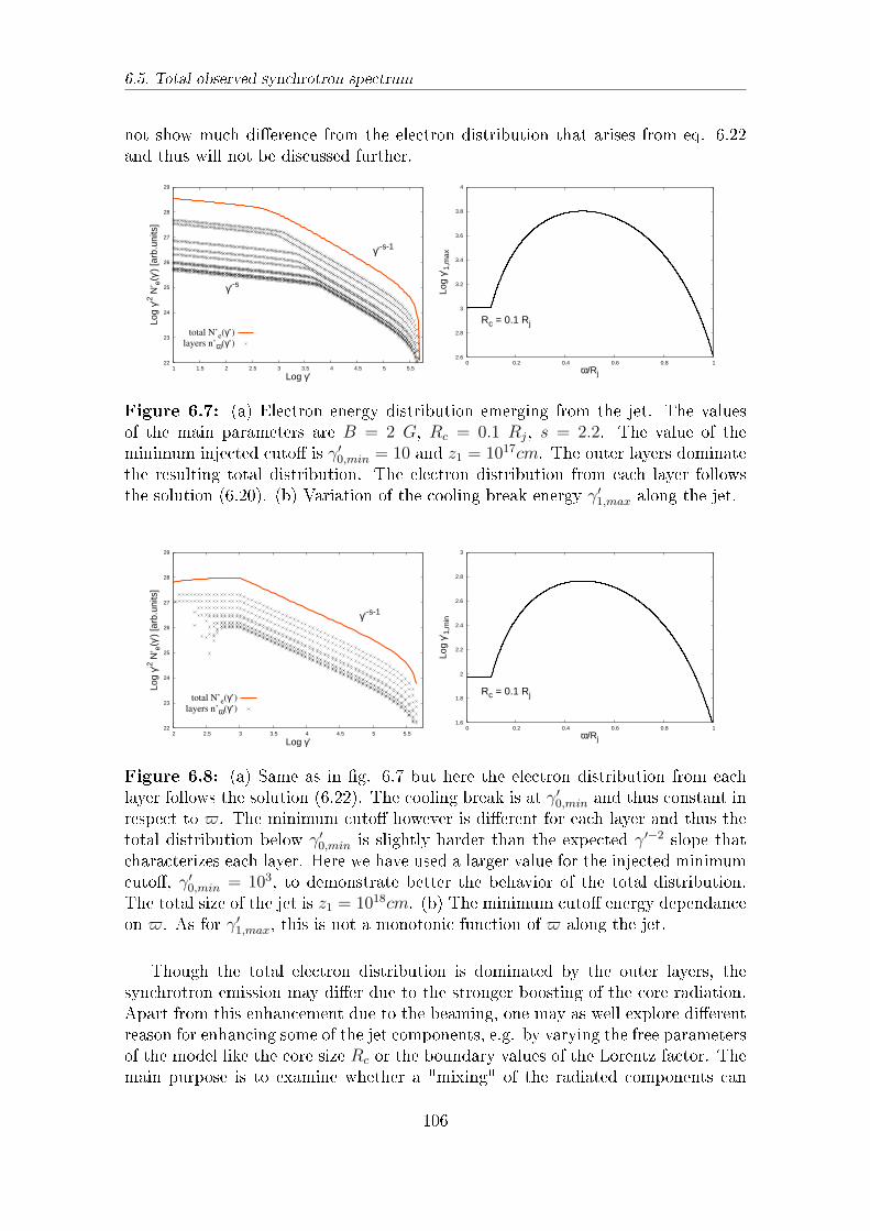
6.5. Total observed synchrotron spectrum
not show much dierence from the electron distribution that arises from eq. 6.22and thus will not be discussed further.
22
23
24
25
26
27
28
29
1 1.5 2 2.5 3 3.5 4 4.5 5 5.5
Log
γ’2 N’ e
(γ’)
[arb
.uni
ts]
Log γ’
γ’-s-1
γ’-s
total N’e(γ’)
layers n’ϖ(γ’)
2.6
2.8
3
3.2
3.4
3.6
3.8
4
0 0.2 0.4 0.6 0.8 1
Log
γ’ 1,m
ax
ϖ/Rj
Rc = 0.1 Rj
Figure 6.7: (a) Electron energy distribution emerging from the jet. The valuesof the main parameters are B = 2 G, Rc = 0.1 Rj, s = 2.2. The value of theminimum injected cuto is γ′
0,min = 10 and z1 = 1017cm. The outer layers dominatethe resulting total distribution. The electron distribution from each layer followsthe solution (6.20). (b) Variation of the cooling break energy γ′
1,max along the jet.
22
23
24
25
26
27
28
29
2 2.5 3 3.5 4 4.5 5 5.5
Log
γ’2 N’ e
(γ’)
[arb
.uni
ts]
Log γ’
γ’-s-1
total N’e(γ’)
layers n’ϖ(γ’)
1.6
1.8
2
2.2
2.4
2.6
2.8
3
0 0.2 0.4 0.6 0.8 1
Log
γ’ 1,m
in
ϖ/Rj
Rc = 0.1 Rj
Figure 6.8: (a) Same as in g. 6.7 but here the electron distribution from eachlayer follows the solution (6.22). The cooling break is at γ′
0,min and thus constant inrespect to ϖ. The minimum cuto however is dierent for each layer and thus thetotal distribution below γ′
0,min is slightly harder than the expected γ′−2 slope thatcharacterizes each layer. Here we have used a larger value for the injected minimumcuto, γ′
0,min = 103, to demonstrate better the behavior of the total distribution.The total size of the jet is z1 = 1018cm. (b) The minimum cuto energy dependanceon ϖ. As for γ′
1,max, this is not a monotonic function of ϖ along the jet.
Though the total electron distribution is dominated by the outer layers, thesynchrotron emission may dier due to the stronger boosting of the core radiation.Apart from this enhancement due to the beaming, one may as well explore dierentreason for enhancing some of the jet components, e.g. by varying the free parametersof the model like the core size Rc or the boundary values of the Lorentz factor. Themain purpose is to examine whether a "mixing" of the radiated components can
106
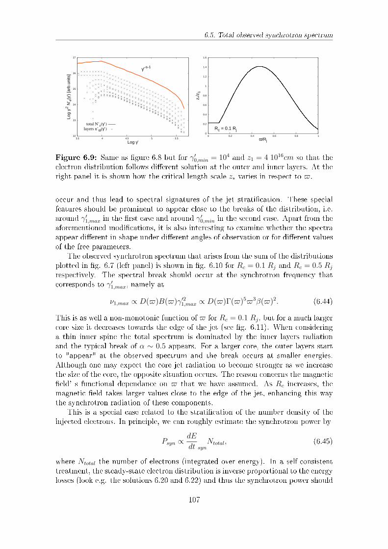
6.5. Total observed synchrotron spectrum
22
23
24
25
26
27
3.5 4 4.5 5 5.5
Log
γ’2 N’ e
(γ’)
[arb
.uni
ts]
Log γ’
γ’-s-1
total N’e(γ’)
layers n’ϖ(γ’) 0
0.2
0.4
0.6
0.8
1
1.2
1.4
1.6
0 0.2 0.4 0.6 0.8 1
z */z
1
ϖ/Rj
Rc = 0.1 Rj
Figure 6.9: Same as gure 6.8 but for γ′0,min = 104 and z1 = 4 1016cm so that the
electron distribution follows dierent solution at the outer and inner layers. At theright panel it is shown how the critical length scale z∗ varies in respect to ϖ.
occur and thus lead to spectral signatures of the jet stratication. These specialfeatures should be prominent to appear close to the breaks of the distribution, i.e.around γ′
1,max in the rst case and around γ′0,min in the second case. Apart from the
aforementioned modications, it is also interesting to examine whether the spectraappear dierent in shape under dierent angles of observation or for dierent valuesof the free parameters.
The observed synchrotron spectrum that arises from the sum of the distributionsplotted in g. 6.7 (left panel) is shown in g. 6.10 for Rc = 0.1 Rj and Rc = 0.5 Rj
respectively. The spectral break should occur at the synchrotron frequency thatcorresponds to γ′
1,max, namely at
ν1,max ∝ D(ϖ)B(ϖ)γ′21,max ∝ D(ϖ)Γ(ϖ)5ϖ3β(ϖ)2. (6.44)
This is as well a non-monotonic function of ϖ for Rc = 0.1 Rj, but for a much largercore size it decreases towards the edge of the jet (see g. 6.11). When consideringa thin inner spine the total spectrum is dominated by the inner layers radiationand the typical break of α ∼ 0.5 appears. For a larger core, the outer layers startto "appear" at the observed spectrum and the break occurs at smaller energies.Although one may expect the core jet radiation to become stronger as we increasethe size of the core, the opposite situation occurs. The reason concerns the magneticeld' s functional dependance on ϖ that we have assumed. As Rc increases, themagnetic eld takes larger values close to the edge of the jet, enhancing this waythe synchrotron radiation of these components.
This is a special case related to the stratication of the number density of theinjected electrons. In principle, we can roughly estimate the synchrotron power by
Psyn ∝ dE
dt synNtotal, (6.45)
where Ntotal the number of electrons (integrated over energy). In a self-consistenttreatment, the steady-state electron distribution is inverse proportional to the energylosses (look e.g. the solutions 6.20 and 6.22) and thus the synchrotron power should
107
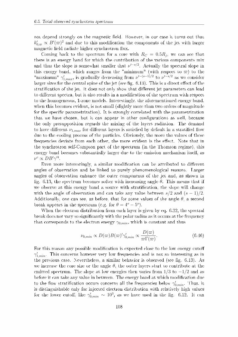
6.5. Total observed synchrotron spectrum
not depend strongly on the magnetic eld. However, in our case it turns out thatk′0,ϖ ∝ B′(ϖ)2 and due to this modication the components of the jet with largermagnetic eld radiate higher synchrotron ux.
Coming back to the spectrum for a core with RC = 0.5Rj, we can see thatthere is an energy band for which the contribution of the various components mixand thus the slope is somewhat smaller that ν ′−s/2. Actually the spectral slope inthis energy band, which ranges from the "minimum" (with respect to ϖ) to the"maximum" γ′
1,max, is gradually decreasing from ν ′−(s−1)/2 to ν ′−s/2 as we considerlarger sizes for the central spine of the jet (see g. 6.13). This is a direct eect of thestratication of the jet. It does not only show that dierent jet parameters can leadto dierent spectra, but it also results in a modication of the spectrum with respectto the homogeneous, 1-zone models. Interestingly, the aforementioned energy band,when this becomes evident, is not small (slightly more than two orders of magnitudefor the specic parametrization). It is strongly correlated with the parametrizationthat we have chosen, but it can appear in other congurations as well, becausethe only presupposition regards the mixing of the layers radiation. The demandto have dierent ν1,max for dierent layers is satised by default in a stratied owdue to the cooling process of the particles. Obviously, the more the values of thesefrequencies deviate from each other, the more evident is the eect. Note that inthe synchrotron self-Compton part of the spectrum (in the Thomson regime), thisenergy band becomes substantially larger due to the emission mechanism itself, asνc ∝ DB′γ′4.
Even more interestingly, a similar modication can be attributed to dierentangles of observation and be linked to purely phenomenological reasons. Largerangles of observation enhance the outer components of the jet and, as shown ing. 6.13, the spectrum becomes softer with increasing angle θ. This means that ifwe observe at this energy band a source with stratication, the slope will changewith the angle of observation and can take any value between s/2 and (s − 1)/2.Additionally, one can see, as before, that for some values of the angle θ, a secondbreak appears in the spectrum (e.g. for θ = 4o − 5o).
When the electron distribution from each layer is given by eq. 6.22, the spectralbreak does not vary so signicantly with the polar radius as it occurs at the frequencythat corresponds to the electron energy γ0,min, which is constant and thus
ν0,min ∝ D(ϖ)B(ϖ)′γ′0,min ∝ D(ϖ)
ϖΓ(ϖ). (6.46)
For this reason any possible modication is expected close to the low energy cutoγ′1,min. This concerns however very low frequencies and is not so interesting as inthe previous case. Nevertheless, a similar behavior is observed (see g. 6.13). Aswe increase the core size or the angle θ, the outer layers start to contribute at theemitted spectrum. The slope at low energies then varies from 1/3 to −1/2 and asbefore it can take any value in between. The energy band at which modication dueto the ow stratication occurs concerns all the frequencies below γ′
0,min. Thus, itis distinguishable only for injected electron distribution with relatively high valuesfor the lower cuto, like γ′
0,min ∼ 103, as we have used in the g. 6.12. It can
108
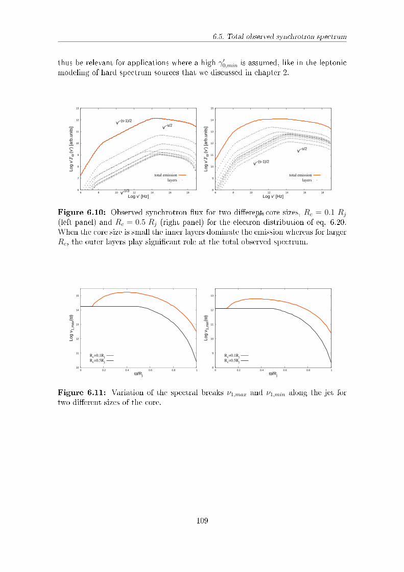
6.5. Total observed synchrotron spectrum
thus be relevant for applications where a high γ′0,min is assumed, like in the leptonic
modeling of hard spectrum sources that we discussed in chapter 2.
6
7
8
9
10
11
12
13
6 8 10 12 14 16 18
Log
v’J’
ϖ (v
’) [a
rb.u
nits
]
Log v’ [Hz]
v’-s/2v’-(s-1)/2
v’1/3
total emission
layers
8
9
10
11
12
13
14
15
6 8 10 12 14 16 18
Log
v’J’
ϖ (v
’) [a
rb.u
nits
]
Log v’ [Hz]
v’-s/2
v’-(s-1)/2
v’1/3
total emission
layers
Figure 6.10: Observed synchrotron ux for two dierent core sizes, Rc = 0.1 Rj
(left panel) and Rc = 0.5 Rj (right panel) for the electron distribution of eq. 6.20.When the core size is small the inner layers dominate the emission whereas for largerRc, the outer layers play signicant role at the total observed spectrum.
10
11
12
13
14
15
0 0.2 0.4 0.6 0.8 1
Log
ν 1,m
ax(ϖ
)
ϖ/Rj
Rc=0.1Rj
Rc=0.5Rj
8
9
10
11
12
13
0 0.2 0.4 0.6 0.8 1
Log
ν 1,m
in(ϖ
)
ϖ/Rj
Rc=0.1Rj
Rc=0.5Rj
Figure 6.11: Variation of the spectral breaks ν1,max and ν1,min along the jet fortwo dierent sizes of the core.
109
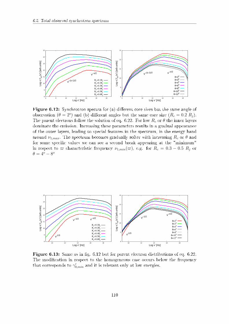
6.5. Total observed synchrotron spectrum
8
9
10
11
12
13
14
15
6 8 10 12 14 16 18
Log
v’J’
ϖ (v
’) [a
rb.u
nits
]
Log v’ [Hz]
v’-s/2
v’-(s-1)/2 Rc=0.1Rj
Rc=0.2Rj
Rc=0.3Rj
Rc=0.4Rj
Rc=0.5Rj
Rc=0.6Rj 8
9
10
11
12
13
6 8 10 12 14 16 18
Log
v’J’
ϖ (v
’) [a
rb.u
nits
]
Log v’ [Hz]
v’-s/2v’-(s-1)/2
θ=2ο
θ=3ο
θ=4ο
θ=6ο
θ=8ο
θ=10ο
θ=12ο
Figure 6.12: Synchrotron spectra for (a) dierent core sizes but the same angle ofobservation (θ = 2o) and (b) dierent angles but the same core size (Rc = 0.2 Rj).The parent electrons follow the solution of eq. 6.22. For low Rc or θ the inner layersdominate the emission. Increasing these parameters results in a gradual appearanceof the outer layers, leading to special features in the spectrum, in the energy bandaround ν1,max. The spectrum becomes gradually softer with increasing Rc or θ andfor some specic values we can see a second break appearing at the "minimum"in respect to ϖ characteristic frequency ν1,min(ϖ), e.g. for Rc = 0.3 − 0.5 Rj orθ = 4o − 8o
8
9
10
11
12
13
14
15
10 12 14 16 18
Log
v’J’
ϖ (v
’) [a
rb.u
nits
]
Log v’ [Hz]
v’-s/2v’-1/2
v’1/3
Rc=0.1Rj
Rc=0.2Rj
Rc=0.3Rj
Rc=0.4Rj
Rc=0.5Rj
Rc=0.6Rj 8
9
10
11
12
13
10 12 14 16 18
Log
v’J’
ϖ (v
’) [a
rb.u
nits
]
Log v’ [Hz]
v’-s/2
v’-1/2
v’1/3
θ=2o
θ=3o
θ=4o
θ=6o
θ=8o
θ=10o
θ=12o
Figure 6.13: Same as in g. 6.12 but for parent electron distributions of eq. 6.22.The modication in respect to the homogeneous case occurs below the frequencythat corresponds to γ′
0,min and it is relevant only at low energies.
110
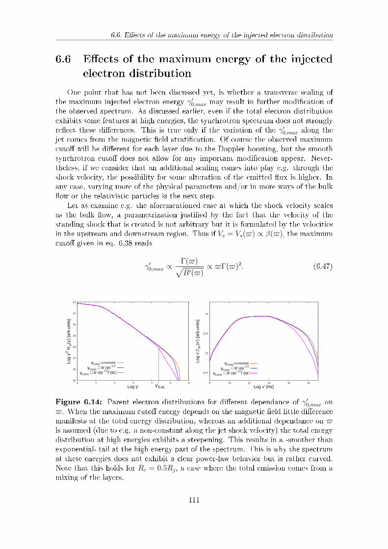
6.6. Eects of the maximum energy of the injected electron distribution
6.6 Eects of the maximum energy of the injected
electron distribution
One point that has not been discussed yet, is whether a transverse scaling ofthe maximum injected electron energy γ′
0,max may result in further modication ofthe observed spectrum. As discussed earlier, even if the total electron distributionexhibits some features at high energies, the synchrotron spectrum does not stronglyreect these dierences. This is true only if the variation of the γ′
0,max along thejet comes from the magnetic eld stratication. Of course the observed maximumcuto will be dierent for each layer due to the Doppler boosting, but the smoothsynchrotron cuto does not allow for any important modication appear. Never-theless, if we consider that an additional scaling comes into play e.g. through theshock velocity, the possibility for some alteration of the emitted ux is higher. Inany case, varying more of the physical parameters and/or in more ways of the bulkow or the relativistic particles is the next step.
Let as examine e.g. the aforementioned case at which the shock velocity scalesas the bulk ow, a parametrization justied by the fact that the velocity of thestanding shock that is created is not arbitrary but it is formulated by the velocitiesin the upstream and downstream region. Thus if Vs = Vs(ϖ) ∝ β(ϖ), the maximumcuto given in eq. 6.38 reads
γ′0,max ∝
Γ(ϖ)√B′(ϖ)
∝ ϖΓ(ϖ)2. (6.47)
25
26
27
28
29
30
31
32
0 1 2 3 4 5 6
Log
γ’2 N’ e
(γ’)
[arb
.uni
ts]
Log γ’ γ’0,ϖ*
γ0,max=constant
γ0,max ∝ B’(ϖ)-1/2
γ0,max ∝ B’(ϖ)-1/2Γ(ϖ) 12.5
13
13.5
14
8 10 12 14 16 18
Log
v’J’
ϖ (v
’) [a
rb.u
nits
]
Log v’ [Hz]
γ0,max=constant
γ0,max ∝ B’(ϖ)-1/2
γ0,max ∝ B’(ϖ)-1/2Γ(ϖ)
Figure 6.14: Parent electron distributions for dierent dependance of γ′0,max on
ϖ. When the maximum cuto energy depends on the magnetic eld little dierencemanifests at the total energy distribution, whereas an additional dependance on ϖis assumed (due to e.g. a non-constant along the jet shock velocity) the total energydistribution at high energies exhibits a steepening. This results in a -smother thanexponential- tail at the high energy part of the spectrum. This is why the spectrumat these energies does not exhibit a clear power-law behavior but is rather curved.Note that this holds for Rc = 0.5Rj, a case where the total emission comes from amixing of the layers.
111
6.7. Summary and future work on stratied outows
Again, the values for the free parameters are to dene whether some featureswill appear at the spectrum due to the mixing of the inner and outer layers of thejet. At g. 6.14 the total electron energy distribution and the observed synchrotronspectrum is shown for Rc = 0.5Rj. Three cases are plotted. A constant γ′
0,max,a dependance only on the magnetic eld according to eq. (6.38) and additionaldependance on ϖ due to the stratication of the shock velocity (eq. 6.47). Whenthe maximum injected energy depends only on the magnetic eld little modicationis observed in respect to the γ′
0,max = constant case. On the other hand, for eq.6.47 both electrons and synchrotron radiation are altered at high energies. Theresulting particle distribution becomes steeper, around the minimum -in respect toϖ- injected energy γ′
0,ϖ∗ . The observed spectrum is steeper as well, but smootherthan the exponential cuto. In total it looks rather curved and does not have a clearpower-law behavior.
6.7 Summary and future work on stratied outows
In this last chapter we have developed a non-homogeneous model for radiationfrom relativistic outows. We discussed only the synchrotron radiation componentof the spectrum, neglecting the ICS component and the corresponding energy losses.Such a scheme allows as to examine in detail the eects of stratication, as we candevelop an analytic solution for the electron distribution in each layer. We haveshown that even in this simplied picture, important deviation from the one zonemodels may appear. Two eects exhibit the underlying stratication. First, theobserved synchrotron spectrum appears dierent for dierent values (of some) ofthe free parameters of the model, e.g. the size of the central core or the angle ofobservation. The main reason concerns the dominance of dierent layers each time.As far as the viewing angles is concerned, this means that intrinsically identical jetsappear dierent for dierent angles, an eect that has been previously discussed inmore simplied cases like the spine-layer model of Ghisellini et al. (2005).
Secondly, we have shown that a mixing of the emission of the layers may occur,leading to interesting features of the spectrum. Within an energy band which (forthe parameters chosen here) extends for ∼ 2 orders of magnitude, the slope of thespectrum can take any value between −s/2 and −(s+1)/2 and it depends purely onthe stratication of the physical parameters. Furthermore, the observed spectrummay show a second break which is an observational evidence for a stratied ow, asit is not expected for homogeneous models. This happens when the injected electrondistribution has a relatively low minimum cuto (γ′
0,min ∼ 10) and the particles donot completely cool before they escape at the edge of the jet. When the injectedcuto is higher so that the local electron distribution from each layer exhibit thecharacteristic∝ γ′−2 behavior, modication analog to the aforementioned is observedat the low energy part of the spectrum. The slope takes arbitrary values among 1/3and −0.5, but no break shows up.
One may then conclude that even within this simplied scheme, a modication ofthe spectrum is expected and may potentially explain spectral features that the ho-mogeneous models fail to interpret. Thus, further development by including the ICS
112
6.7. Summary and future work on stratied outows
component is desired, as these modication may either be enhanced or smoothedout. In both cases evidence for stratication is strong as normally the two com-ponents of the spectrum are assumed to be similar, i.e. exhibit roughly the samepower-law slope. Deviation from the standard assumptions usually made, homo-geneity and/or isotropy can be proved signicant for explaining peculiar featuresof the radiated spectra within leptonic models and without extreme phenomenolog-ical assumptions. Additionally, the possible stratication of a relativistic outowis closely related to the MHD processes that take place and thus its manifestationthrough the emission mechanisms provides an interesting tool for testing or com-paring current theoretical models.
113

6.7. Summary and future work on stratied outows
114
Chapter 7
Conclusions
In this thesis we have investigated the leptonic radiation processes that take placein the relativistic outows of AGN. We have developed a self-consistent approachshedding light on a number of unsolved problems regarding the interpretation of theobserved spectra, and we have expanded current models in order to examine morecomplex, non-homogeneous congurations. Furthermore, we have analyzed in detailissues related to the spectral shape of the emitted radiation.
One major topic in AGN physics that has attracted attention over the last yearsis the interpretation of the hard VHE Blazar spectra. After correction for EBLinteraction of the emitted TeV photons, the intrinsic spectra of some sources appearparticularly hard, possessing challenges to standard leptonic models. In chapter 2
we have discussed the capability of narrow electron distributions to explain suchhard spectra. We have shown that these distributions within a self-consistent, timedependent treatment, can lead to the formation of hard spectra. A power-law witha large value of the low-energy cuto can be maintained in the presence of energylosses if adiabatic losses due to the expansion of the source control the evolutionof electrons at low energies. Furthermore, stochastic acceleration of particles incombination with radiation losses, naturally leads to the formation of relativisticMaxwell-type distributions which can successfully explain even extremely hard VHEBlazar spectra.
Interestingly, narrow particle distributions such as Maxwellian type distribu-tions can account for broader spectra as well, once they are embedded in a non-homogeneous, multi-zone scenario. In chapter 3 we have developed a phenomeno-logical model in which the emitted Blazar spectra originates from several regions(blobs), where electrons are stochastically accelerated to relativistic energies. Theresultant emission can lead to power-law like spectra, with index simply controlledby the energetics of the blobs. In this scheme, if one (or few) of the blobs becomemore energetic (due to either an increase of the injected energy or an enhancementof the Doppler boosting), hard aring events can be satisfactorily interpreted. Inparticular, such "leading blob" scenario can account for the characteristic Mkn 501are in 2009 during which a strong spectral hardening was observed.
The radiated spectra in the aforementioned cases (and in general in the lit-erature) are calculated numerically. The kernel functions of the synchrotron and
115
Chapter 7. Conclusions
Compton processes are complex and the full convolution with the particle distribu-tion can not be handled analytically. However, analytical approximations are veryimportant, as they give a helpful insight into the underlying physics, especially theacceleration of the particles. In chapter 4 we develop analytical approximationsthat describe the shape of the Compton spectrum close to the high-energy cuto.The high-energy cuto of the electron distribution carries crucial information ofthe acceleration process and can be used to distinguish among current theories. Ourcalculations provide a direct link between the parent electrons and the emitted spec-trum. Additionally, we can draw some general conclusions. For example, we showthat the shape of the two components of the observed spectrum (the low energy,synchrotron bump and the high energy Compton bump) are not always identical. Inparticular, in the Thomson regime the cuto shape depends strongly on the targetphoton eld, and is rather broad, which is not the case in the Klein-Nishina regimewhere the spectral cuto resembles the shape of the electron distribution and ismore sharp.
The calculation of the observed Blazar spectra are essentially related to theDoppler boosting of the emitted radiation. Blazars are known to exhibit relativis-tic jets and the relativistic motion can lead to an important enhancement of theintrinsic luminosity. Interestingly, the beaming pattern depends on the emissionprocess, e.g. it is dierent for the synchrotron/SSC and EC model. In chapter 5 wesolve the photon transfer equation in order to obtain the formulas that describe theDoppler boosting for general electron distributions, non-homogeneous, anisotropicand stationary. These calculations generalize the results previously obtained in theliterature. Furthermore, they allow us to examine the interesting case of anisotropicparticle distributions that are often predicted in acceleration theories. We show thatthe anisotropy of the radiating particles may lead to a possible mis-estimation of theDoppler factor, as the luminosity peaks at viewing angles dierent than in the caseof isotropic models. Under the natural assumption that the degree of anisotropydepends on the energy of the particles, we show that the emitted synchrotron spec-trum may appear harder. This eect is even more evident in the EC componentand in total anisotropy can introduce modication of these two components.
In principle, relaxing standard assumptions, i.e. anisotropy or homogeneity ofthe emitting source, has important consequences for understanding peculiar featuresof the observed spectra. We have seen in chapter 3 that within a phenomenolog-ical non-homogeneous model, hard aring events can be interpreted under certainassumption. We have also shown in chapter 5 that the emitted spectral shape candier substantially from the case of isotropic particles and thus it can account forspectra that the same power-law distributions can not explain in the isotropic case.In chapter 6 we examine a non-homogeneous model in which the parameters of thesource vary continuously, as inferred from MHD simulations. In particular, we de-velop a self-consistent approach for the synchrotron radiation that emerges from astratied jet. The stratication arises in the transverse (to the uid velocity) direc-tion and it concerns several physical parameters, such as the bulk Lorentz factor, themagnetic eld, the energy density of the parent electrons as well as the value of themaximum cuto of the particle distribution. In our scheme, the relativistic electrons
116
Chapter 7. Conclusions
are assumed to be injected in the radiation zone at the base of the jet. We showthat such a stratication may lead to interesting dierences with respect to homo-geneous models. First of all, as discussed before in more simplied inhomogeneousmodels, the spectrum may appear dierent for dierent viewing angles. Secondly,the observed spectrum can exhibit special features related to the stratication. Forexample, an additional break in the SED, which is related to the cooling break thatthe particle distribution exhibits in each layer. The stratication may be as wellrevealed through the spectral slope of a part of the spectrum, which is not relatedto the acceleration process, but depends on the assumed relations that describe theparameters' stratication.
The noted time-dependent approaches, as well as the deviation from standardassumptions, such as isotropy and homogeneity, oer important insight for the non-thermal emission from AGN jets and allow to successfully address a number ofunsolved problems. Leptonic models have more to reveal for the AGN physics thanoften assumed.
117

Chapter 7. Conclusions
118
Bibliography
Abdo, A.A. et al. 2011, ApJ, 727, 129
Aharonian, F.A. 2000, NewA, 5, 377
Aharonian, F., Akhperjanian, A. G., Barres de Almeida, U., et al. 2007, A&A, 473,L25
Aharonian, F., Akhperjanian, A. G., Bazer-Bachi, A. R., et al. 2007, ApJL, 664,L71
Aharonian, F. A., & Ambartsumyan, A. S. 1985, Astrophysics, 23, 650
Aharonian F. A. & Atoyan, A. M. 1981, Ap&SS, 79, 321
Aharonian, F.A., Atoyan, A. M., & Nahapetian, A. 1986, A&A, 162, L1
Aharonian, F. A., Kelner, S. R. & Prosekin, A. Yu. 2010, PhRvD, 82d 3002A
Aharonian, F.A., Khangulyan, D., & Costamante, L. 2008, MNRAS, 387, 1206
Aharonian, F.A., Timokhin, A.N., & Plyasheshnikov, A.V. 2002, A&A, 384, 834
Aharonian, F., et al. 2006, Nature, 440, 1081
Aharonian, F., et al. 2007, A&A, 475, L9
Aharonian, F., Akhperjanian, A. G., Bazer-Bachi, A. R., et al. 2007, ApJL, 664,L71
Aharonian, F., et al., 2007a, A&A, 470, 475
Aharonian, F., et al., 2007b, A&A, 475, L9
Albert, J., Aliu, E., Anderhub, H., et al. 2007, ApJ, 669, 862
Aleksi¢, J., Antonelli, L. A., Antoranz, P., et al. 2011, A&A, 530, A4
Alfvén, H., & Herlofson, N. 1950, Physical Review, 78, 616
Aloy, M.-A., Gomez, J.-L., Ibanez, J.-M., Marti, J.-M., Muller, E. 2000, ApJL, 528,L85
Aloy, M. A., & Mimica, P. 2008, ApJ, 681, 84
Antonucci, R. 1993, ARA & A, 31, 473
119
BIBLIOGRAPHY BIBLIOGRAPHY
Appl, S., & Camenzind, M. 1993, A&A, 274, 699
Atoyan A. M., & Aharonian F. A. 1999, MNRAS, 302, 253
Attridge, J. M., Roberts, D. H., & Wardle, J. F. C. 1999, ApJL, 518, L87
Axford, W. I., Leer, E., & Skadron, G. 1978, Cosmophysics, 125
Becker, P. A., Das, S., & Le, T. 2008, ApJL, 677, L93
Bednarek, W., Kirk, J. G., & Mastichiadis, A. 1996, A&A, 307, L17
Begelman, M.C., Blandford, R.D., & Rees, M.J. 1984, Reviews of Modern Physics,56, 255
Bell, A. R. 1978, MNRAS, 182, 443
Blandford, R. D., & Levinson, A. 1995, ApJ, 441, 79
Blandford, R. D., & Ostriker, J. P. 1978, ApJL, 221, L29
Blandford, R. D., & Payne, D. G. 1982, MNRAS, 199, 883
Blandford, R. D., & Rees, M. J. 1974, MNRAS, 169, 395
Blandford, R. D., & Znajek, R. L. 1977, MNRAS, 179, 433
Bloom, S.D. & Marscher A.P. 1996, ApJ, 461, 657
Blumenthal, G. R. 1971, Phys. Rev. D, 3, 2308.
Blumenthal, G. R., & Gould, R. J. 1970, Reviews of Modern Physics, 42, 237
Boettcher, M. 2012, arXiv:1205.0539
Böttcher, M., Dermer, C.D., & Finke, J.D. 2008, ApJ, 679, L9
Brunetti, G. 2000, Astropart. Phys., 13, 107
Celotti, A., & Blandford, R. D. 2001, Black Holes in Binaries and Galactic Nuclei,206
Cerutti, B., Werner, G. R., Uzdensky, D. A., & Begelman, M. C. 2012,arXiv:1205.3210
Chiaberge, M., Celotti, A., Capetti, A., & Ghisellini, G. 2000, A& A, 358, 104
Coppi, P. S. & Blandford, R. D. 1990, MNRAS., 245, 453
Costamante, L. 2012, IAU Symposium, 284, 420
Crusius, A., & Schlickeiser, R. 1986, A&A, 164, L16
De Angelis, A., Mansutti, O., Persic, M., & Roncadelli, M. 2009, MNRAS, 394, L21
Derishev, E. V. 2007, Ap&SS, 309, 157
Derishev, E.V., Aharonian, F.A., Kocharovsky, V.V., Kocharovsky, Vl. V. 2003,Phys. Rev. D, 68, 043003
120
BIBLIOGRAPHY BIBLIOGRAPHY
Derishev, E. V., Aharonian, F. A., & Kocharovsky, V. V. 2007, ApJ, 655, 980
Dermer, C. D. 1995, ApJL, 446, L63
Dermer, C. D., & Atoyan, A. M. 2002, ApJ, 568, L81
Dermer, C. D., Schlickeiser, R., & Mastichiadis, A. 1992, A&A, 256, L27
Dermer, C. D., & Schlickeiser, R. 1993, ApJ, 416, 458
Dempsey, P., & Duy, P. 2007, MNRAS, 378, 625
Dominguez, A., Primack, J. R., Rosario, D. J., et al. 2010, MNRAS, 410, 2556
Domínguez, A., Primack, J. R., Rosario, D. J., et al. 2011, MNRAS, 410, 2556
Eilek, J. A., & Arendt, P. N. 1996, ApJ, 457, 150
Eilek, J. A., Melrose, D. B., & Walker, M. A. 1997, ApJ, 483, 282
Epstein, R. I. 1973, ApJ, 183, 593
Epstein, R. I., & Petrosian, V. 1973, ApJ, 183, 611
Essey, W., & Kusenko, A. 2012, ApJL, 751, L11
Essey, W., & Kusenko, A. 2010, Astroparticle Physics, 33, 81
Essey, W., Kalashev, O. E., Kusenko, A., & Beacom, J. F. 2010, Physical ReviewLetters, 104, 141102
Essey, W., Kalashev, O., Kusenko, A., & Beacom, J. F. 2011 ApJ, 731 51E
Fermi, E. 1949, Physical Review, 75, 1169
Fermi, E. 1954, ApJ, 119, 1
Franceschini, A., Rodigliero, G., & Vaccari, M. 2008, A&A, 487, 837
Frank J., King A., Raine D., 1995, Accretion Power in Astrophysics, (second edi-tion), Cambridge Univ. Press: Cambridge
Fritz, K.D. 1989, A&A, 214, 14
Georganopoulos, M., & Kazanas, D. 2003, ApJL, 594, L27
Georganopoulos, M., Kirk, J.G., & Mastichiadis, A. 2001, ApJ, 561, 111
Ghisellini, G., Tavecchio, F., & Chiaberge, M. 2005, A&A, 432, 401
Giebels, B., Dubus, G., & Khéli, B. 2007, A&A, 462, 29
Gilmore, R. C., Somerville, R. S., Primack, J. R., & Domínguez, A. 2012, MNRAS,422, 3189
Giovannini, G., Cotton, W. D., Feretti, L., Lara, L., & Venturi, T. 1998, arXiv:astro-ph/9808261
121
BIBLIOGRAPHY BIBLIOGRAPHY
Giovannini, G., Cotton, W. D., Feretti, L., Lara, L., & Venturi, T. 1999, MmSAI,70, 161
Giovannini, G., Cotton, W. D., Feretti, L., Lara, L., & Venturi, T. 2001, ApJ, 552,508
Gomez, J. L., Marti, J. M. A., Marscher, A. P., Ibanez, J. M. A., & Marcaide, J. M.1995, ApJL, 449, L19
Gould, R.J., & Schreder, G.P. 1967, Physical Review, 155, 1408
Gracia, J., Vlahakis, N., Agudo, I., Tsinganos, K., & Bogovalov, S. V. 2009, ApJ,695, 503
Hardcastle, M. J., Alexander, P., Pooley, G. G., & Riley, J. M. 1997, MNRAS, 288,L1
Hauser, M. G., & Dwek, E. 2001, ARA&A, 39, 249
Henri, G., & Pelletier, G. 1991, ApJL, 383, L7
Hooper, D., & Serpico, P. D. 2007, Physical Review Letters, 99, 231102
Jackson, J. D. 1975, 92/12/31, New York: Wiley, 1975, 2nd ed.,
Jones, F.C. 1968, Phys.Rev., 167, 1159
Jones, T. W., O'dell, S. L., & Stein, W. A. 1974, ApJ, 188, 353
Kahn, F. D. 1983, MNRAS, 202, 553
Katz-Stone, D. M., & Rudnick, L. 1994, ApJ, 426, 116
Kardashev, N. S. 1962, SvA, 6, 317
Katarzy«ski, K., Ghisellini, G., Tavecchio, F., Gracia, J., & Maraschi, L. 2006,MNRAS, 368, L52
Khangulyan, D. & Aharonian, F. 2005, AIPC 745, 359K
Kifune, T. 1999, ApJL, 518, L21
King, A. 2012, arXiv:1201.2060
Kneiske, T. M., Bretz, T., Mannheim, K., & Hartmann, D. H. 2004, A&A, 413, 807
Krawczynski, H., Coppi, C.S., & Aharonian, F. 2002, MNRAS, 336, 721
Komissarov, S. S. 1990, Soviet Astronomy Letters, 16, 284
Komissarov, S. S., Barkov, M. V., Vlahakis, N., Konigl, A. 2007, MNRAS, 380, 51
Krymskii G.F., 1977, Akademiia Nauk SSSR, Doklady 234, 1306
Kusunose, M., & Takahara, F. 2005, ApJ, 621, 285
Laing, R. A. 1996, Energy Transport in Radio Galaxies and Quasars, 100, 241
122
BIBLIOGRAPHY BIBLIOGRAPHY
Laing, R. A., Canvin, J. R., Cotton, W. D., & Bridle, A. H. 2006, MNRAS, 368, 48
Laing, R. A., Canvin, J. R., Bridle, A. H., & Hardcastle, M. J. 2006, MNRAS, 372,510
Laing, R. A., Parma, P., de Ruiter, H. R., & Fanti, R. 1999, MNRAS, 306, 513
Laing, R. A., & Bridle, A. H. 2002, MNRAS, 336, 328
Laing, R. A., Canvin, J. R., & Bridle, A. H. 2006, Astronomische Nachrichten, 327,523
Lazarian, A., Kowal, G., Pino, B. G. d., & Vishniac, E. T. 2012, Multi-scale Dy-namical Processes in Space and Astrophysical Plasmas, 11
Lefa, E., Rieger, F. M., & Aharonian, F. 2011, ApJ, 740, 64
Lefa, E., Aharonian, F. A., & Rieger, F. M. 2011, ApJL, 743, L19
Lefa, E., Kelner, S. R., & Aharonian, F. A. 2012, ApJ, 753, 176
Lenain, J.-P., Boisson, C., Sol, H. & Katarzy«ski, K., 2008, A&A 478, 111
Li, H.-Q., Wang, J.-C., & Xue, L. 2004, ChJaa, 4, 311
Li, H., & Wang, J. 2004, ApJ, 617, 162
Lind, K. R., & Blandford, R. D. 1985, ApJ, 295, 358
Longair, M. S. 2010, High Energy Astrophysics by Malcolm S. Longair. CambridgeUniversity Press, 2010. ISBN: 9780521756181,
Lovelace, R. V. E. 1976, Nature, 262, 649
Lynden-Bell, D. 1978, Phys. Scripta, 17, 185
Madejski, G. M. 1999, arXiv:astro-ph/9903141
Mannheim, K. 1993, A&A, 269, 67
Mannheim, K., & Biermann, P. L. 1992, A&A, 253, L21
Mandal, S., & Chakrabarti, S. K. 2008, ApJL, 689, L17
Massaro, E., Tramacere, A., Perri, M., Giommi, P., & Tosti, G. 2006, A&A, 448,861
Maraschi, L., Ghisellini, G., & Celotti, A. 1992, ApJL, 397, L5
Medvedev, M. V. 2006, ApJ, 637, 869
Melrose, D. B. 1980, Plasma astrophysics: Nonthermal processes in diuse magne-tized plasmas, Astrophysical applications (New York, Gordon and Breach SciencePublishers), 2, 430
Moderski, R., Sikora, M., Coppi, P. S., & Aharonian, F. 2005, MNRAS 363, 954
Morrison, P., Sadun, A., & Roberts, D. 1984, ApJ, 280, 483
123
BIBLIOGRAPHY BIBLIOGRAPHY
Narginen D. I. & Putanen, J. 1993, A&A, 275, 325
Neronov, A., Semikoz, D., & Taylor, A. M. 2012, A&A, 541, A31
Owen, F. N., Hardee, P. E., & Cornwell, T. J. 1989, ApJ, 340, 698
Padovani, P. 1999, Vulcano Workshop 1998: Frontier Objects in Astrophysics andParticle Physics, 159
Perlman, E. S., Biretta, J. A., Zhou, F., Sparks, W. B., & Macchetto, F. D. 1999,AJ, 117, 2185
Petrosian, V. 2012, Space Sci. Rev., 49
Phinney, E. S. 1982, MNRAS, 198, 1109
Primack, J. R. et al. 2011, Proc. of the 25th Texas Symposium (eds. F.A. Aharonian,W. Hofmann, F.M. Rieger), AIP Conf. Proc. 1381, in press (arXiv:1107.2566)
Protheroe, R. J. 1997, IAU Colloq. 163: Accretion Phenomena and Related Out-ows, 121, 585
Perucho, M., & Martí, J. M. 2007, MNRAS, 382, 526
Piran, T. 1982, ApJL, 257, L23
Poutanen, J., & Vurm, I. 2010, ApJS, 189, 286
Prosekin, A., Essey, W., Kusenko, A., & Aharonian, F. 2012, arXiv:1203.3787
Rees, M. J. 1966, Nature, 211, 468
Reid, M. J., Biretta, J. A., Junor, W., Muxlow, T. W. B., Spencer, R. E. 1989ApJ,336, 112R
Reville, B., & Kirk, J. G. 2010, ApJ, 724, 1283
Rieger, F.M. 2004, ApJ, 615, L5
Rieger, F.M., Bosch-Ramon, V., & Duy, P. 2007, Ap&SS, 309, 119
Rieger, F. M., & Duy, P. 2004, ApJ, 617, 155
Runi, R., & Wilson, J. R. 1975, Phys. Rev. D, 12, 2959
Rybicki, G. B., & Lightman, A. P. 1979, Radiative Processes in Astrophysics (NewYork: Wiley)
Salpeter, E. E. 1964, ApJ, 140, 796
Saugé, L., & Henri, G. 2006, A&A, 454, L1
Sauty, C., Tsinganos, K., & Trussoni, E. 2002, Relativistic Flows in Astrophysics,589, 41
Sazonov S. Y. & Sunyaev, R. A. 2000, ApJ, 543, 28
Schlickeiser, R. 1985, A&A, 143, 431
124
BIBLIOGRAPHY BIBLIOGRAPHY
Schmidt M., 1963, Nature 197, 1040
Shakura, N. I., & Sunyaev, R. A. 1973, A&A, 24, 337
Sikora, M., Begelman, M. C., & Rees, M. J. 1994, ApJ, 421, 153
Sikora, M., Blazejowski, M., Moderski, R., & Madejski, G. M. 2002, ApJ, 577, 78
Sikora, M., Madejski, G., Moderski, R., & Poutanen, J. 1997, ApJ, 484, 108
Sikora, M., Sol, H., Begelman, M. C., & Madejski, G. M. 1996, MNRAS, 280, 781
Skilling, J. 1975, MNRAS, 172, 557
Stawarz, ., & Ostrowski, M. 2002, ApJ, 578, 763
Stawarz, L., Aharonian, F., Wagner, S., & Ostrowski, M. 2006, MNRAS, 371, 1705
Stawarz, L., & Petrosian, V. 2008, ApJ, 681, 1725
Stawarz, L., Petrosian, V., & Blandford, R. D. 2010, ApJ, 710, 236
Stecker, F.W., Baring, M. G. & Summerlin, E. J. 2007, ApJL, 667, L29.
Stecker, F.W., & Glashow, S.L. 2001, Astropart. Phys. 16, 97
Stecker, F. W., & Scully, S. T. 2008, A&A, 478, L1
Sturrock, P. A. 1966, Physical Review, 141, 186
Syrovatskii, S. I. 1959, SvA, 3, 22
Tavecchio, F., & Ghisellini, G. 2008, MNRAS, 385, L98
Tavecchio, F., Ghisellini, G., Ghirlanda, G., Costamante, L., & Franceschini, A.2009, MNRAS, 399, L59
Tavecchio, F., Maraschi, L., & Ghisellini, G. 1998, ApJ, 509, 608
Urry, C.M., & Padovani, P. 1995, PASP, 107, 803
Vannoni, G., Gabici, S., & Aharonian, F. A. 2009, A&A 497, 17V
Vlahakis, N., Königl, A. 2003, ApJ, 596, 1080
Webb, G. M., Drury L. O'C., Biermann, P. 1984, A&A, 137, 185
Yang, J., Wang, J., Dai, B., & Gao, X. 2009, PASJ, 61, 1153
Zacharopoulou, O., Khangulyan, D., Aharonian, F., & Costamante, L. 2011, ApJin press
Zeldovich, Y., & Novikov, I. 1964, Sov. Phys. Dokl., 158, 811
Zirakashvili, V.N., & Aharonian, F. 2007, A&A, 465, 695
Zdziarski, A. A. 1989, ApJ, 342, 1108
125

BIBLIOGRAPHY BIBLIOGRAPHY
126
Acknowledgements
First of all I would like to thank my supervisors, Dr. Frank Rieger and prof. FelixAharonian, without whom this thesis would not be possible. I deeply thank FrankRieger who has greatly motivated me for several astrophysical research themes, hehas imparted to me his fascination and enthusiasm for astrophysics through manyinspiring discussions, and he has introduced me to the art of scientic writing. Hisadvising but also his kindness, support and patience have been invaluable. I amalso extremely grateful to Felix Aharonian, the guidance of whom helped me totransform from an ignorant student to a young researcher. The critical sight intoseveral research topics and the deep understanding of them are among the pricelessthings I learned from him. For sure, I could not hope for better supervisors. Iwould also like to sincerely thank prof. Stanislav Kelner who has kindly taught meanalytical and mathematical technics. Learning from him has proven to be amongthe most valuable skills I obtained during these years. I would like also to thank prof.Werner Hofmann for his kindness to be the referee of this thesis and for his patience.I also thank prof. Matthias Bartelmann and prof. Eva Grebel for accepting to bemy exam committee. I am indebted to Christian Fendt who accepted to be part ofmy thesis committee and has always oered his help, whenever I needed it.
I am very grateful to many people associated to the High Energy Astrophysicsgroup in MPI-K, who helped me a lot with my research and made my everyday lifein the institute so enjoyable. My sincere gratitude to Emma De Ona Wihelmi forher help and advices on the observational part and for being such a wonderful friend.My thanks also to Maxim Barkov for issues related to MHD, Valenti Bosch-Ramonand Mytia Khangulian for their help on radiation processes. I want also to verymuch thank Sabrina Casanova for her cheerfulness, Roland Crocker for the helpwith Mathematica, Victor Zabaltza for the interesting discussions, those who haveleft already, David Jones Andrew Taylor, but also Luigi Costamante for many nicediscussions, and profs. Heinz Völk, John Kirk and Stefan Wagner, and of course myphd fellows, Ervin Kafexhiou for all the help with the computer, Anton Prosenkinand Ruizhi Yang for their support and all of them for the kikker fun.
I would like to deeply thank the wonderful friends in Heidelberg, that made mystay here an experience of life. Emma once again for everything, Vivi for being like asister to me, my great atmates Claudia, Paula, Romanski for all the fun and mostimportant for all the sharing, Nikos for becoming such close friend, Marta for allthe laugh, the British Toby, Adam and Matt for their wonderful company, Andy ofcourse, Michael for many many things and Christian. I would also like to speciallythank my close family, my mother Popi and my sister Ismini for their support andunconditional love that proved so important. And my step-father Marios, withoutwhom I would not be what I am. And Tzesi for taking care of them. And I own alot to my beloved friends back home, Tzo kirofaki, Pagio and Gaki, Hara, Evi, NikoSkivalo, Michali and Marianthi, George Pappas, Mitso, my cousin Giota and Giorgo
127
and my sweet Artemis, little Helen and all my big family; all of them supported intheir own special way this phd. I also want to deeply thank my Alex for his love,which has been a home to me. Last, I own a gratitude to my rst teacher, ManolisKapetanakis, who motivated and supported me so much for studying physics.
This thesis is dedicated to my father, Chris, and to my step-father, Marios, whotaught me the most important of all; life.
128
List of publications
Refereed Journals
1. Lefa, E., Rieger, F. M., & Aharonian, F. 2011, ApJ, 740, 64"Formation of Very Hard Gamma-Ray Spectra of Blazars in Leptonic Models"
2. Lefa, E., Aharonian, F. A., & Rieger, F. M. 2011, ApJL, 743, L19"Leading Blob Model in a Stochastic Acceleration Scenario: The Case of the 2009Flare of Mkn 501"
3. Lefa, E., Kelner, S. R., & Aharonian, F. A. 2012, ApJ, 753, 176"On the Spectral Shape of Radiation due to Inverse Compton Scattering Close tothe Maximum Cuto"
Conference proceedings
1. Lefa, E., Rieger, F. M., & Aharonian, F. 2010,25th Texas Symposium on Relativistic Astrophysics,"The formation of hard TeV gamma-ray spectra in Blazars" (poster)
2. Lefa, E., Rieger, F., & Aharonian, F. 2011,AGN Physics in the CTA Era (AGN 2011),"Hard VHE γ-ray spectra in Blazars" (talk)
3. Lefa, E., Rieger, F. M., & Aharonian, F. A. 2012,International Journal of Modern Physics Conference Series, 8, 31 "Hard Gamma-RaySource Spectra in TeV Blazars" (talk)
129