thermodynamics · 1.2. an axiomatic approach to thermodynamics thermodynamics addresses macroscopic...
TRANSCRIPT
ThermodynamicsStefan Schorsch, Marco Mazzotti∗
ETH Zurich, Institute of Process Engineering, Sonneggstrasse 3, CH-8092 Zurich, Switzerland
Preface
What is Chemical Engineering about? According to the AIChE (the biggest
association of chemical engineers) it is the profession in which a knowledge of
mathematics, chemistry, and other natural sciences gained by study, experience,
and practice i s applied with j udgment to develop economic ways of using
materials and energy f or the benefit of mankind. As this i s a rather broad
definition, quite a few fields do belong to chemical engineering such as chemical
reactions, separation processes, biological reactions, research on
thermodynamics, energy con-version, solids processing, fluid dynamics, and
construction and design of equip-ment. Many industrial fields apply chemical
engineering knowledge such as the chemical-, food-, pharmaceutical-, energy-, or
automotive industries. These notes aim at giving you a first impression and an
overview over these fields by studying the following specific topics: phase
equilibrium thermodynamics, liquid-vapor equilibria and liquid-solid equilibria.
∗Corresponding author: phone +41 44 632 2456; fax +41 44 632 11 41.Email address: [email protected] (Marco Mazzotti)
Preprint submitted to Script April 11, 2017
Contents
1 Thermodynamics and Phase Equilibria 4
1.1 Introduction . . . . . . . . . . . . . . . . . . . . . . . . . . . . . . 4
1.2 An axiomatic approach to thermodynamics . . . . . . . . . . . . 4
1.2.1 Four Postulates . . . . . . . . . . . . . . . . . . . . . . . . 4
1.2.2 Entropy Representation . . . . . . . . . . . . . . . . . . . 6
1.2.3 Internal Energy Representation . . . . . . . . . . . . . . . 7
1.3 Thermodynamic Equilibrium . . . . . . . . . . . . . . . . . . . . 7
1.3.1 Thermal Equilibrium . . . . . . . . . . . . . . . . . . . . . 8
1.3.2 Mechanical Equilibrium . . . . . . . . . . . . . . . . . . . 10
1.3.3 Equilibrium with respect to mass transfer . . . . . . . . . 11
1.4 Euler Equation . . . . . . . . . . . . . . . . . . . . . . . . . . . . 15
1.5 Legendre Transformations . . . . . . . . . . . . . . . . . . . . . . 18
1.6 Cross Derivatives . . . . . . . . . . . . . . . . . . . . . . . . . . . 24
1.7 Gibbs Phase Rule . . . . . . . . . . . . . . . . . . . . . . . . . . . 25
1.8 Pure Ideal Gases . . . . . . . . . . . . . . . . . . . . . . . . . . . 29
1.9 Pure Real Gases . . . . . . . . . . . . . . . . . . . . . . . . . . . 30
1.9.1 Compressibility . . . . . . . . . . . . . . . . . . . . . . . . 31
1.9.2 Van-der-Waals EOS . . . . . . . . . . . . . . . . . . . . . 31
1.9.3 Virial EOS . . . . . . . . . . . . . . . . . . . . . . . . . . 32
1.10 Fugacity . . . . . . . . . . . . . . . . . . . . . . . . . . . . . . . . 33
1.11 Fugacity in the Liquid Phase - Single Component Vapor Liquid
Equilibrium (VLE) . . . . . . . . . . . . . . . . . . . . . . . . . . 36
1.12 Mixtures . . . . . . . . . . . . . . . . . . . . . . . . . . . . . . . . 40
1.12.1 Vapor Liquid Equilibrium for mixtures . . . . . . . . . . . 46
1.12.2 Fugacity in solutions: Osmotic pressure and reverse osmosis 47
1.12.3 Volume of a mixture . . . . . . . . . . . . . . . . . . . . . 50
2
1.12.4 Chemical equilibrium . . . . . . . . . . . . . . . . . . . . 51
1.13 Liquid vapor equilibrium in binary mixtures . . . . . . . . . . . . 56
1.13.1 LVE in single component systems . . . . . . . . . . . . . . 56
1.13.2 P-xy diagrams . . . . . . . . . . . . . . . . . . . . . . . . 56
1.13.3 T-xy diagrams . . . . . . . . . . . . . . . . . . . . . . . . 63
1.13.4 x-y diagrams . . . . . . . . . . . . . . . . . . . . . . . . . 64
1.13.5 H-xy diagrams . . . . . . . . . . . . . . . . . . . . . . . . 67
1.13.6 Azeotropes . . . . . . . . . . . . . . . . . . . . . . . . . . 69
3
1. Thermodynamics and Phase Equilibria
1.1. Introduction
In this section we provide the basis for the study of thermodynamic equilib-
rium for systems involving multiple chemical species and multiple phases. This
requires extending the thermodynamics presented in previous classes (namely
Thermodynamics I given by Prof. Poulikakos in the HS 2012; chapters 2, 6 and
8 of the corresponding script are particularly useful), which was more focused
on single component systems.
1.2. An axiomatic approach to thermodynamics
Thermodynamics addresses macroscopic systems and processes related to
heat, energy, and work consisting of a gargantuan number of elementary objects,
either atoms or molecules, i.e. of the order of the Avogadro number, NA =
6 × 10²³. While classical thermodynamics is based on the first and the second
law, which were first established through experimental observations and then
plugged into a theoretical framework, our approach is axiomatic. We start
from four postulates that establish a mathematical framework consistent with
the physical reality, in which all thermodynamics can be developed rigorously.
The justification of this approach is that chemical engineers need dealing with
multicomponent multiphase systems, involving quantities that are much more
difficult to observe and measure than those involved in for instance simple heat
transfer problems.
1.2.1. Four Postulates
1st postulate. Simple systems at equilibrium are completely characterized by
the following extensive properties: internal energy U , volume V , and number of
moles n1, n2, . . . , nC of each of the C components i, with index i = 1, 2, . . . , C.
4
Simple systems are characterized as such by being macroscopically homoge-
neous, isotropic, electrically neutral, chemically inert, under no external field
influence, and large enough to neglect surface effects.
For an extensive property its value U for a system consisting of the combination
of a number of subsystems is equal to the sum of the values U (j) of the same
property for each subsystem j, i.e.: U = ΣjU(j), etc.
2nd postulate. At equilibrium, there exists a function S defined in terms of
the extensive quantities above, i.e. S = S(U, V, n1, n2, . . . , nC), which is called
entropy. This is the so-called entropy representation.
At equilibrium the quantities U , V , n1, . . ., nC attain values, which must at
the same time be compatible with the external constraints and maximize the
entropy S. Therefore at equilibrium, S is maximum, dS = 0 and d2S < 0.
3rd postulate. The entropy S is also an extensive property, i.e. S = ΣjS(j). If
this is applied to λ identical subsystems, the Euler formula is derived:
S(λU, λV, λn1, λn2, . . . , λnC) = λS(U, V, n1, n2, . . . , nC). (1)
Moreover, S is a continuous, differentiable, and monotonically increasing func-
tion of U , i.e. (∂S/∂U)V,ni> 0. As a consequence S can be inverted, and
the internal energy U can be expressed as a function of S, V , n1, . . ., nC , i.e.
U = U(S, V, n1, n2, . . . , nC). This is the so-called internal energy representation.
4th postulate. The entropy is zero when:
S = 0↔(∂U
∂S
)V,ni
= 0 (2)
This condition applies at a temperature T =0 K, i.e. at the absolute zero
temperature.
5
Four postulates
1. Simple systems at equilibrium are defined by their U ,V ,n1, n2, ..., nC .
2. S = S(U, V, n1, n2, ..., nC); U ,V ,n1, n2, ..., nC attain values compatible
with the external constraints that maximize S → dS = 0;d2S < 0
3. S is extensive, i.e. S =∑j Sj ; S is continuous, differentiable, monotonically
increasing function of U → U representation: U = U(S, V, n1, n2, ..., nC)
4. S = 0↔ (∂U/∂S)V,n1,n2,...,nC= 0→ S = 0 at T = 0 K
1.2.2. Entropy Representation
According to the 2nd postulate:
S = S(U, V, n1, n2, . . . , nC); (3)
therefore its differential is given as:
dS =
(∂S
∂U
)V,ni
dU +
(∂S
∂V
)U,ni
dV +
C∑i=1
(∂S
∂ni
)U,V,nj 6=i
dni (4)
All partial derivatives in the equation above are intensive properties. If the
system under consideration is split into a number of subsystems, all subsystems
exhibit the same intensive properties of the original system, whereas their ex-
tensive properties, such as V or U or ni, are equal to that of the original system
multiplied by the ratio between the size of the subsystem and that of the origi-
nal system. We will see when introducing the conditions for thermodynamical
equilibrium that among the intensive properties there are system temperature
T and system pressure P , which are obviously the same for all parts of the
original homogeneous system.
6
1.2.3. Internal Energy Representation
Let us consider the function defining the internal energy U (see the 3rd
postulate):
U = U(S, V, n1, n2, . . . , nC); (5)
its differential is:
dU =
(∂U
∂S
)V,ni
dS +
(∂U
∂V
)S,ni
dV +
C∑i=1
(∂U
∂ni
)S,V,nj 6=i
dni (6)
1.3. Thermodynamic Equilibrium
The fundamental problem of thermodynamics can be described as follows.
Given a composite system, isolated from the external world, what is its final
equilibrium state after some of the internal constraints are removed? For ex-
ample, if in a closed system consisting of two subsytems A and B, a rigid,
adiabatic, impermeable wall is suddenly replaced by a rigid, impermeable, but
heat conducting wall, what will be the final temperature of the two subsys-
tems? Or alternatively, what happens if the same wall is replaced by a rigid but
permeable wall (a membrane) instead?
We will analyze thermodynamic equilibrium using the entropy and internal
energy representations introduced above, and we will see that the partial deriva-
tives of the entropy function play a crucial role. For the sake of simplicity, we
will recast the differential form of the entropy function as follows:
dS = α︸︷︷︸( ∂S
∂U )V,ni
dU + β︸︷︷︸( ∂S
∂V )U,ni
dV +
C∑i=1
γi︸︷︷︸(∂S∂ni
)U,V,nj 6=i
dni (7)
We will investigate three different cases to derive conditions for thermal, me-
chanical, and equilibrium with respect to mass transfer.
7
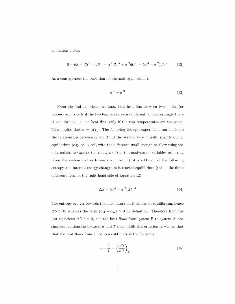
1.3.1. Thermal Equilibrium
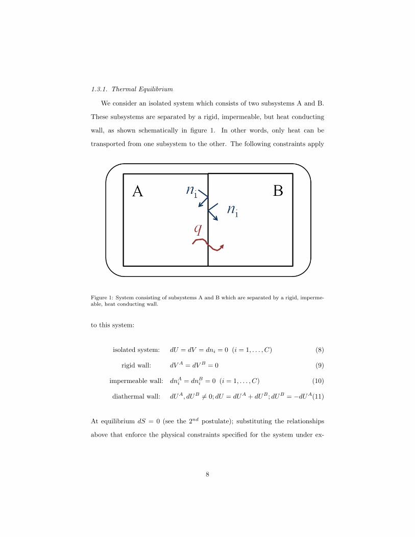
We consider an isolated system which consists of two subsystems A and B.
These subsystems are separated by a rigid, impermeable, but heat conducting
wall, as shown schematically in figure 1. In other words, only heat can be
transported from one subsystem to the other. The following constraints apply
Figure 1: System consisting of subsystems A and B which are separated by a rigid, imperme-able, heat conducting wall.
to this system:
isolated system: dU = dV = dni = 0 (i = 1, . . . , C) (8)
rigid wall: dV A = dV B = 0 (9)
impermeable wall: dnAi = dnBi = 0 (i = 1, . . . , C) (10)
diathermal wall: dUA, dUB 6= 0; dU = dUA + dUB ; dUB = −dUA(11)
At equilibrium dS = 0 (see the 2nd postulate); substituting the relationships
above that enforce the physical constraints specified for the system under ex-
8
amination yields:
0 = dS = dSA + dSB = αAdUA + αBdUB = (αA − αB)dUA (12)
As a consequence, the condition for thermal equilibrium is:
αA = αB (13)
From physical experience we know that heat flux between two bodies (or
phases) occurs only if the two temperatures are different, and accordingly there
is equilibrium, i.e. no heat flux, only if the two temperatures are the same.
This implies that α = α(T ). The following thought experiment can elucidate
the relationship between α and T . If the system were initially slightly out of
equilibrium (e.g. αA > αB , with the difference small enough to allow using the
differentials to express the changes of the thermodynamic variables occurring
when the system evolves towards equilibrium), it would exhibit the following
entropy and internal energy changes as it reaches equilibrium (this is the finite
difference form of the right hand side of Equation 12):
∆S = (αA − αB)∆UA (14)
The entropy evolves towards the maximum that it attains at equilibrium, hence
∆S > 0, whereas the term (αA − αB) > 0 by definition. Therefore from the
last equations ∆UA > 0, and the heat flows from system B to system A. the
simplest relationship between α and T that fulfills this criterion as well as that
that the heat flows from a hot to a cold body is the following:
α =1
T=
(∂S
∂U
)V,ni
. (15)
9
Accordingly TA = TB at equilibrium and entropy has the units of an energy
per unit temperature change, i.e. J/K.
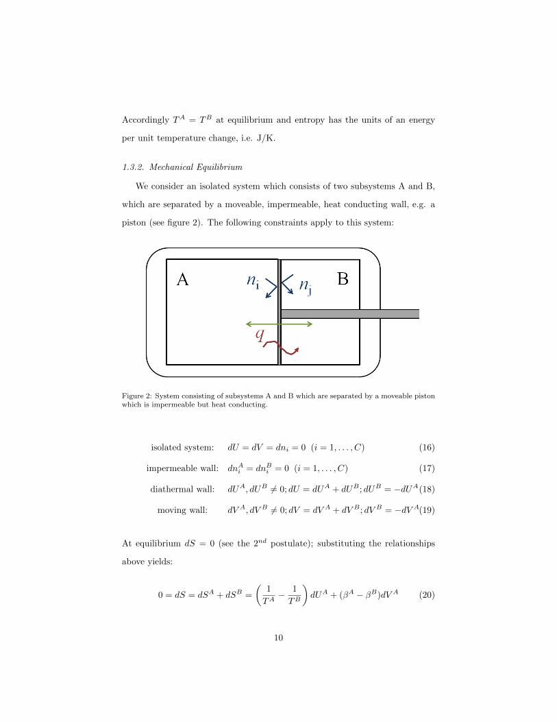
1.3.2. Mechanical Equilibrium
We consider an isolated system which consists of two subsystems A and B,
which are separated by a moveable, impermeable, heat conducting wall, e.g. a
piston (see figure 2). The following constraints apply to this system:
Figure 2: System consisting of subsystems A and B which are separated by a moveable pistonwhich is impermeable but heat conducting.
isolated system: dU = dV = dni = 0 (i = 1, . . . , C) (16)
impermeable wall: dnAi = dnBi = 0 (i = 1, . . . , C) (17)
diathermal wall: dUA, dUB 6= 0; dU = dUA + dUB ; dUB = −dUA(18)
moving wall: dV A, dV B 6= 0; dV = dV A + dV B ; dV B = −dV A(19)
At equilibrium dS = 0 (see the 2nd postulate); substituting the relationships
above yields:
0 = dS = dSA + dSB =
(1
TA− 1
TB
)dUA + (βA − βB)dV A (20)
10
Since TA = TB , the condition for mechanical equilibrium is:
βA = βB . (21)
Equilibrium in this case is of a mechanical nature, and is associated to an
equilibrium of forces, which in this example implies that the pressures in the two
chambers (subsystems) are the same; therefore β depends on pressure. Since
β = (∂S/∂V )U,ni, it has the units of energy per unit temperature change and
unit volume, i.e. the units of a pressure per unit temperature change. The
simplest definition of β that is consistent with these conditions is:
β =P
T=
(∂S
∂V
)U,ni
(22)
Since we already know that at equilibrium TA = TB , therefore mechanical
equilibrium requires that PA = PB .
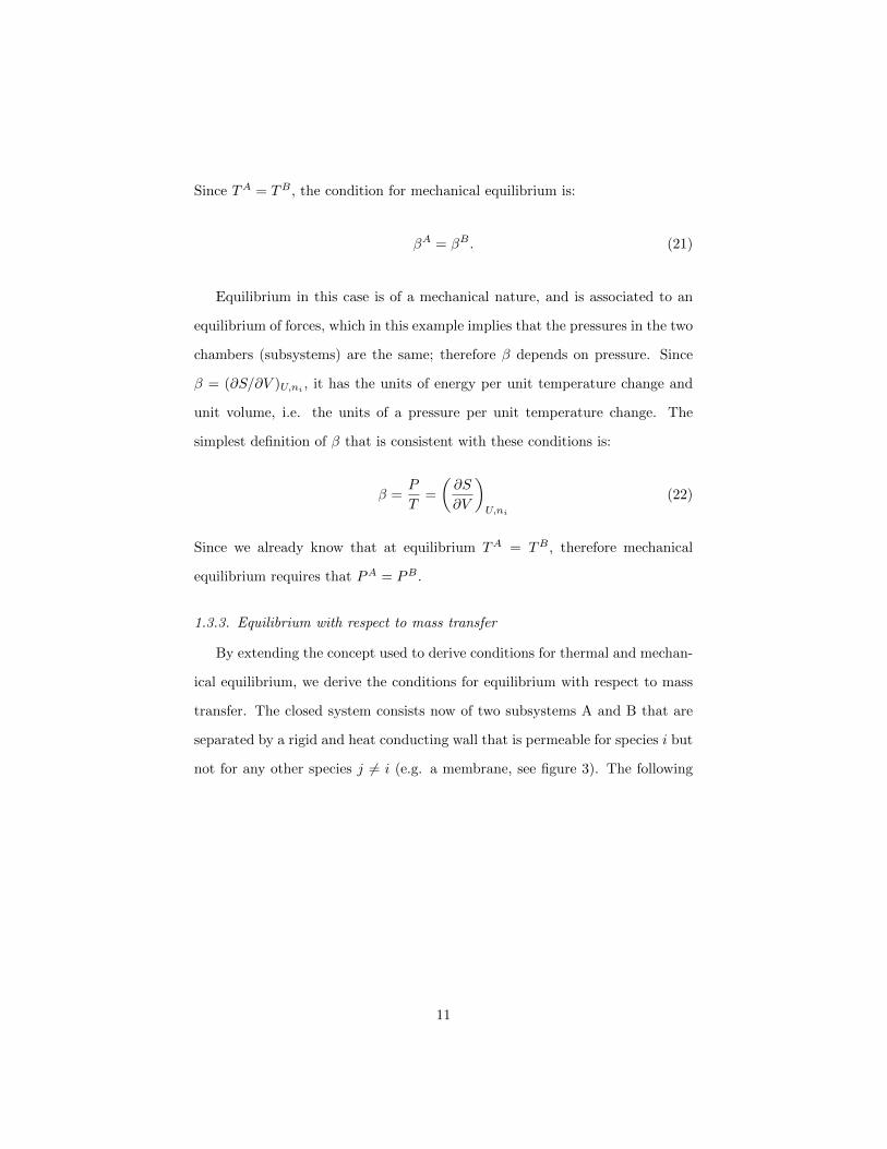
1.3.3. Equilibrium with respect to mass transfer
By extending the concept used to derive conditions for thermal and mechan-
ical equilibrium, we derive the conditions for equilibrium with respect to mass
transfer. The closed system consists now of two subsystems A and B that are
separated by a rigid and heat conducting wall that is permeable for species i but
not for any other species j 6= i (e.g. a membrane, see figure 3). The following
11
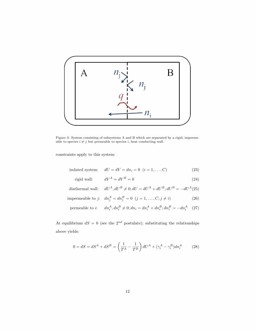
Figure 3: System consisting of subsystems A and B which are separated by a rigid, imperme-able to species i 6= j but permeable to species i, heat conducting wall.
constraints apply to this system:
isolated system: dU = dV = dni = 0 (i = 1, . . . , C) (23)
rigid wall: dV A = dV B = 0 (24)
diathermal wall: dUA, dUB 6= 0; dU = dUA + dUB ; dUB = −dUA(25)
impermeable to j: dnAj = dnBj = 0 (j = 1, . . . , C; j 6= i) (26)
permeable to i: dnAi , dnBi 6= 0; dni = dnAi + dnBi ; dnBi = −dnAi (27)
At equilibrium dS = 0 (see the 2nd postulate); substituting the relationships
above yields:
0 = dS = dSA + dSB =
(1
TA− 1
TB
)dUA + (γAi − γBi )dnAi (28)
12
Since at equilibrium TA = TB , then γAi = γBi as well, where:
γi =
(∂S
∂ni
)U,V,nj 6=i
(29)
Neither intuition nor physical observation provide us with a measurable
quantity associated to equilibrium with respect to mass transfer that can play
the same role as temperature or pressure in the cases of thermal or mechanical
equilibrium. It is in fact easy to see that the concentration of the species i in the
two phases cannot be a criterion for equilibrium with respect to mass transfer.
It follows that the quantity γi defined through the derivative in the last equation
is indeed the decisive property in this context. For a number of reasons, includ-
ing the fact that mass transfer cannot be decoupled from heat transfer, a new
quantity, the chemical potential µi of species i has been introduced according
to the following definition:
γi =−µiT
=
(∂S
∂ni
)U,V,nj 6=i
. (30)
According to this definition the chemical potential µi is a specific energy, i.e. it
has units of energy per mole or J/mol. Since temperature has to be the same at
equilibrium, also the chemical potential of the species that can be transferred
from one subsystem to the other has to be the same in the two subsystems,
i.e. µAi = µBi . Finally, the minus sign in the definition of µi stems from the
requirement that mass flows from the subsystem with the larger µi value to that
with the smaller µi value. This can be verified by a similar thought experiment
like the one discussed in the context of thermal equilibrium. If we assume a
slight initial unbalance with µAi > µBi but TA = TB (i.e. the two subsystems
are already at thermal equilibrium) and we calculate the entropy change upon
13
attainment of equilibrium, we obtain:
∆S =
(−µAiTB
− −µBi
TB
)∆nAi (31)
Since ∆S must be positive and the term between brackets is negative by defini-
tion, then also ∆nAi < 0 thus implying that molecules of species i are transported
from subsystem A to subsystem B as required.
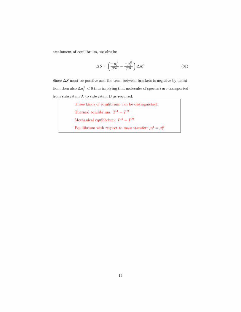
Three kinds of equilibrium can be distinguished:
Thermal equilibrium: TA = TB
Mechanical equilibrium: PA = PB
Equilibrium with respect to mass transfer: µAi = µBi
14
Using the results above, we can obtain a new expression for the total differ-
ential of the entropy function S:
dS =1
T︸︷︷︸( ∂S
∂U )V,ni
=α
dU +P
T︸︷︷︸( ∂S
∂V )U,ni
=β
dV +
C∑i=1
(−µiT
)︸ ︷︷ ︸(
∂S∂ni
)U,V,nj 6=i
=γi
dni (32)
By multiplying the equation above by T and solving for the differential of the
internal energy dU one obtains the following expression for the total derivative
of the function U = U(S, V, n1, n2, . . . , nC):
dU = TdS − PdV +
C∑i=1
µidni (33)
Note that this implies:
T =
(∂U
∂S
)V,ni
(34)
−P =
(∂U
∂V
)S,ni
(35)
µi =
(∂U
∂ni
)S,V,nj 6=i
(36)
1.4. Euler Equation
As a postulate we have taken that the entropy is a function of internal energy,
volume, and composition:
S = S(U, V, n1, n2, ...) (37)
15
Considering the three different types of equilibrium, we were able to identify
the meaning of all terms in the total differential so that
dS =1
TdU +
P
TdV −
∑i
µiTdni (38)
or reformulated in the internal energy representation:
dU = TdS − PdV +∑i
µidni (39)
As S,U ,V , and the composition ni are extensive properties one can write for λ
identical subsystems having entropy S = S(U, V, n1, n2, ...) the following rela-
tionship:
S(λU, λV, λn1, λn2, ...) = λS(U, V, n1, n2, ...) (40)
Differentiating this equation by λ yields
∂S
∂(λU)U +
∂S
∂(λV )V +
∑i
∂S
∂(λni)ni = S (41)
This equation is true for all values of λ, hence for λ = 1 we find that
S =U
T+PV
T−∑i
µiniT
(42)
or
U = TS − PV +∑i
µini (43)
Note that these are properties of functions fulfilling Euler equation:
λf(x) = f(λx) (44)
16
For those functions one can always write by differentiating with respect to λ
f(x) = f ′(λx)x = {ifλ = 1} = f ′(x)x (45)
Let us consider the special case with one component only (C = 1⇒ n1 = n) in
which we set λ = 1/n.
S
(U
n,V
n,n
n
)=
1
nS(U, V, n) (46)
The fractions do have a special meaing
• Un : molar internal energy u
• Sn : molar entropy s
• Vn : molar volume v
So we can rewrite
s = S(u, v, 1) = s(u, v) (47)
Accordingly
u = u(s, v) (48)
u, v, s are intensive properties in contrast to the extensive properties U ,V , and
S. The fundamental equations in differential form can be written equivalently:
ds =1
Tdu+
P
Tdv (49)
du = Tds− Pdv (50)
The U -representation and S-representation provide all thermodynamic informa-
tion on a system, but are not very convenient because they have only extensive
17
variables as dependent variables. T and P are easier to handle as, for example,
there exists no device to measure entropy directly. On the other side, there are
many instruments to measure P and T .
Mathematics can be used to derive new potentials (instead of using U or S) to
describe equilibrium that depend on T and P or other quantities instead. The
method is called Legendre transformation which we will discover in the next
section.
1.5. Legendre Transformations
As stated in the first postulate, a system is entirely characterized by the
internal energy U , the volume V , and the composition ni as S(U, V, n1, . . . , nC).
The entropy function S can be inverted which yields the internal energy function
U(S, V, n1, . . . , nC) which also fully characterizes the system. This function
depends on the quantities S, V, ni for i = 1, 2, . . . , C. Some of these are not very
practical if one wants to measure a system in reality (as for example, there is no
method to measure the entropy directly). In this chapter we are investigating
possibilities to change this dependence.
Helmholtz free energy. Let us consider the internal energy U = U(S, V, n1, . . . , nC)
in the differential form:
dU = TdS − PdV +
C∑i=1
µidni (51)
The partial derivative of U with respect to S is
(∂U
∂S
)V,ni
= T = T (S, V, n1, . . . , nC) (52)
18
By inverting the functional form for T we can find a new functional form for S
which we call S.
T (S, V, n1, . . . , nC)→ S = S(T, V, n1, . . . , nC) (53)
If one wants to switch S ↔ T , we have two options that are
(I) invert T and S to obtain a new function f :
U = U(S(T, V, n1, . . . , nC), V, n1, . . . , nC) = U(T, V, n1, . . . , nC) (54)
The old functional form U is thus transformed into a new function form U which
does now depend on T rather than S.
For a single component system where C = 1 one finds that U = U(T, V, n).
Using molar quantities one can write u = u(T, v) This approach is of course
valid, however it turns out to be less practical.
(II) The second option to find a functional form which does not depend
on S but instead on T is a Legendre Transformation. Applying a Legendre
Transformation to the internal energy and changing S with T yields a new
quantity called Helmholtz Free Energy A which is defined as:
A = U − S(∂U
∂S
)V,ni
(55)
Using the functions U and S that depend on T , V , and ni allows expressing
also A as a function of these variables:
A = U − T S = A(T, V, n1, . . . , nC) (56)
19
The corresponding differential form is
dA = dU − TdS − SdT = −SdT − PdV +
C∑i=1
µidni (57)
The following properties result:
(∂A
∂T
)V,ni
= −S;
(∂A
∂V
)T,ni
= −P ;
(∂A
∂ni
)V,T,nj 6=i
= µi (58)
In comparison to
U = ST − PV +
C∑i=1
µini (59)
for the Helmholtz free energy:
A = −PV +
C∑i=1
µini (60)
One should observe the symmetry of the partial derivatives (∂U/∂S)V,ni= T
and (∂A/∂T )V,ni= −S. This is a key feature of the Legendre Transformation
and depends on the fact that the new thermodynamic potential A is defined as
the difference between the old potential U and the product of the variables to
be swapped, i.e. S and T . The same concept will now be used to swap V and
P .
Enthalpy. Again considering the internal energy U(S, V, ni) but now looking for
a function to replace V with −P we convert the internal energy to a new state
function called enthalpy H(S, P, ni). First, we consider the partial derivative of
U with respect to V to obtain a new functional form:
P = −(∂U
∂V
)S,ni
= P (S, V, n1, . . . , nC) (61)
20
The enthalpy is then defined as:
H = U − V(∂U
∂V
)S,ni
= U + PV = H(S, P, n1, . . . , nC) (62)
The total differential (starting from H = U + PV ) reads:
dH = dU + PdV + V dP = TdS − PdV +
C∑i=1
µidni + PdV + V dP (63)
which yields
dH = TdS + V dP +
C∑i=1
µidni (64)
As a comparison the following properties hold
(∂H
∂S
)P,ni
= T ;
(∂H
∂P
)S,ni
= V ;
(∂H
∂ni
)P,S,nj 6=i
= µi (65)
Note again the symmetry (∂U/∂V )S,ni = −P and (∂H/∂P )S,ni = V . The
enthalpy is then
H = TS +
C∑i=1
µini (66)
Gibbs Free Energy. The enthalpy H depends on entropy S, pressure P , and
the systems composition ni. We are now looking for a quantity that does only
depend on easy measurable independent variables instead that are P and T . In
order to honor its discoverer this quantity is called Gibbs Free Energy G. We
are seeking a quantity that depends on temperature, pressure and composition
(expressed in number of moles): G = G(T, P, n1, . . . , nC). Applying a Legendre
Transformation on H for exchanging S to T yields (using equations 43 and 62):
G = H − S(∂H
∂S
)P,ni
= H − TS =∑i
µini = G(T, P, n1, ..., nC) (67)
21
The differential yields
dG = dH − TdS − SdT = −SdT + V dP +
C∑i=1
µidni (68)
Therefor the following relationships can be derived:
(∂G
∂T
)P,ni
= −S;
(∂G
∂P
)T,ni
= V ;
(∂G
∂ni
)T,P,nj 6=i
= µi (69)
Note again the symmetry of the partial derivatives (∂H/∂S)P,ni= T and
(∂G/∂T )P,ni = −S.
The last equation in equation 69 is the most important defintion of µi, the
chemical potential of species i. In fact it establishes that µi is the partial molar
Gibbs free energy Gi
Gi =
(∂G
∂ni
)T,P,nj 6=i
= µi(T, P, n1, . . . , nC) (70)
For any thermodynamic quantity M , its partial molar quantity is obtained in
general as
Mi =
(∂M
∂ni
)T,P,nj 6=i
(71)
i.e. as its derivative with respect to ni as constant T ,P and ni with j 6= i.
Please recall that it is the chemical potential which we identified to characterize
thermodynamic equilibrium with respect to mass transfer.
For a single component system where C = 1 the equation above reduces to
G = nµ (72)
and
dG = −SdT + V dP + µdn (73)
22
G =
(∂G
∂n
)T,P
=
(∂(ng)
∂n
)T,P
= g
(∂n
∂n
)T,P
= g (T, P ) = µ (T, P ) (74)
where g is the molar Gibbs free energy g = G/n. At constant n one obtains
dg = dµ = −sdT + vdP (75)
For a multicomponent system taking into account that the sum of all sub-
stances i in a system is
n =
C∑i=1
ni (76)
we can define the molar fraction zi of component i as
zi =nin
(77)
with values of zi between 0 and 1 and∑Ci=1 zi = 1. Please note that due to
convention, a generic molar fraction is referred to using the symbol z; for liquid
phases we use xi and for gas phases yi instead. These molar fractions zi for all
components i = 1, . . . , C can be written as vector z = (z1, z2, . . . , zC)T . Since
µi is an intensive property, therefore
µi(T, P, n1, . . . , nC) = µi(T, P, z1, . . . , zC) = µi(T, P, z) (78)
and we see that µi depends only on intensive properties.
23
Overview over Legendre Transformations:
U(S, V, ni)S↔T→ A(T, V, ni)
U(S, V, ni)V↔P→ H(S, P, ni)
H(S, P, ni)S↔T→ G(T, P, ni)
A(T, V, ni)V↔P→ G(T, P, ni)
1.6. Cross Derivatives
Let us recall the general properties of functions of more than one variable,
e.g. f(x, y). If f is continuous and differntiable in x and y, then the second
order cross-derivatives are the same independent of the order of differentiation,
i.e.
∂2f
∂x∂y=
∂2f
∂y∂x(79)
When this general property is applied to G, one obtains a very important rela-
tionship concerning the dependence of the chemical potential on pressure. From
equation 69, particularly from the second and the third equation, one obtains
(∂µi∂P
)T,ni
=
(∂V
∂ni
)T,P,nj 6=i
= Vi (80)
where the defintion of partial molar volume has been exploited.
In the case of a single component, the last equation reads:
(∂µ
∂P
)T,n
=
(∂V
∂n
)T,P
= v (81)
where v is the molar volume.
24
The Gibbs Free Energy depends only on measurable quantities G = G(T, P, ni)
The derivative of G with respect to the number of moles of component i at
constant temperature, pressure, and number of moles of species j 6= i
defines the chemical potential of component i,
i.e. this defines the condition for equilibrium with respect to mass transfer.
µi only depends on intensive properties µi(T, P, z)
1.7. Gibbs Phase Rule
A phase is a region of a system in which the chemical composition and
physical properties are constant from a macroscopic point of view. Think of
a glass of water with ice in it. The fluid is one phase and the ice is a second
phase. How many phases can coexist in equilibrium? This question can be
answered using the properties that we have exploited within previous chapters.
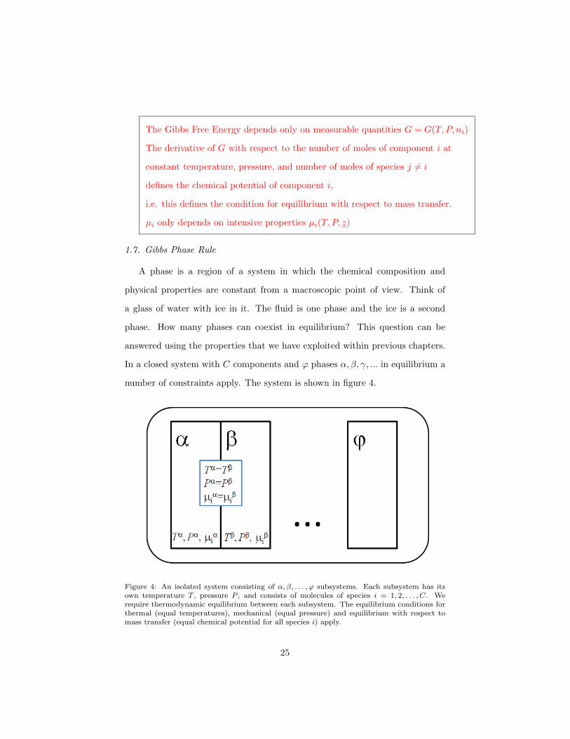
In a closed system with C components and ϕ phases α, β, γ, ... in equilibrium a
number of constraints apply. The system is shown in figure 4.
Figure 4: An isolated system consisting of α, β, . . . , ϕ subsystems. Each subsystem has itsown temperature T , pressure P , and consists of molecules of species i = 1, 2, . . . , C. Werequire thermodynamic equilibrium between each subsystem. The equilibrium conditions forthermal (equal temperatures), mechanical (equal pressure) and equilibrium with respect tomass transfer (equal chemical potential for all species i) apply.
25
Thermal equilibrium requires that:
Tα = T β = ... = Tϕ ⇒ ϕ− 1 equations (82)
Mechanical equilibrium means that:
Pα = P β = ... = Pϕ ⇒ ϕ− 1 equations (83)
Equilibrium with respect to mass transfer requires that the chemical potential
of each substance i is the same in each phase:
µαi = µβi = ... = µϕi i = 1, . . . , C ⇒ C(ϕ− 1) equations (84)
Summing up the number of equations yields Cϕ+ 2ϕ− C − 2. We also have a
number of unknown quantities, i.e. for every phase, T , P and the composition
expressed as molar fraction (Note that∑Ci=1 zi = 1):
Tα, T β , ...Tϕ ⇒ ϕ unknowns (85)
Pα, P β , ...Pϕ ⇒ ϕ unknowns (86)
zαi , zβi , ...z
ϕi i = 1, . . . , C ⇒ ϕ(C − 1) unknowns (87)
The total number of unknowns is therefore ϕ(1 + C). The degrees of freedom
F for the system are therefore
F = ϕ(1 + C)− Cϕ− 2ϕ+ C + 2 (88)
26
F = C + 2− ϕ (89)
This equation is also known as Gibbs Phase Rule. It tells us how many instenive
properties can be manipulated independently without changing the number of
phases. For a single component system, the equation reads for example
F = 3− ϕ (90)
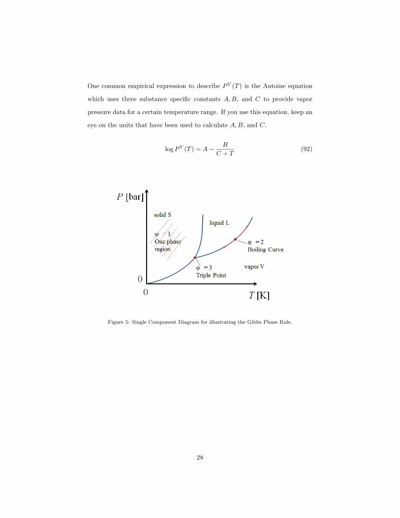
For (see Figure 5)
• ϕ = 1: F=2 ⇒ in a P − T -diagram this is equivalent to an area, i.e. the
solid, liquid, or vapor phase areas;
• ϕ = 2: F=1 ⇒ in a P − T -diagram this is equivalent to a line, e.g. the
boiling curve along the liquid to vapor areas of equilibrium;
• ϕ = 3: F=0 ⇒ in a P − T -diagram this is equivalent to a point, e.g. the
triple point where all three phases are at equilibrium.
Using this knowledge and combining it with a number of measurements one is
able to construct a single component phase diagram. An example is given in
the P − T diagram in figure 5. Two single phase regions are separated from
each other by a line: The boiling curve (vapor-liquid), the sublimation line
(solid-vapor), and the melting line (solid-liquid).
The boiling curve (or vapor pressure curve) will be of central interest in
this lecture. This curve is the pressure exerted by a vapor in thermodynamic
equilibrium with its liquid phase at a given temperature in a closed system. The
vapor pressure is a function of temperature:
PV (T ) (91)
27
One common empirical expression to describe PV (T ) is the Antoine equation
which uses three substance specific constants A,B, and C to provide vapor
pressure data for a certain temperature range. If you use this equation, keep an
eye on the units that have been used to calculate A,B, and C.
logPV (T ) = A− B
C + T(92)
Figure 5: Single Component Diagram for illustrating the Gibbs Phase Rule.
28
The number of degrees of freedom of a system are:
F = C + 2− ϕ
1.8. Pure Ideal Gases
Up to now, we have investigated thermodynamic conditions that define equi-
librium between different phases. Next we will explore single phase regions and
combine these findings with these equilibrium requirements to understand the
behavior of multi-phase systems. We start by considering the gas phase. The
most simple case is the ideal gas which behaves according to the ideal gas law
(an equation of state: EOS). Equations of state define the state of matter in a
certain range of physical conditions and connect state variables (such as tem-
perature, pressure, volume, or internal energy). Such an EOS has the general
form
f(P, T, V, n1, n2, .., nC) (93)
Where does an EOS come from? Taking the fundamental equation for the Gibbs
Free Energy we already found that:
dG = −SdT + V dP +
C∑i=1
µidni (94)
Regarding the behavior of gases, one is particularly interested in the dependence
of the volume on other state variables. The volume can be seen as the derivative
of the Gibbs Free Energy with respect to pressure. The volume itself will depend
on temperature, pressure, and the composition (given in number of moles):
V =
(∂G
∂P
)T,ni
= V (T, P, n1, n2, ..., nC) (95)
We are actually looking for a function which expresses this dependence. The
ideal gas law itself is well known and was found empirically (law of Boyle-
29
Mariotte, laws of Gay-Lussac):
PV = nRT (96)
by dividing the above equation by n we find that
Pv∗ = RT (97)
note that we are now considering the molar volume v instead of the volume V
and that the ∗ indicates that this equation is only true for ideal gases (ideal
gas behavior, see script Prof. Poulikakos section 3.5). As we found out that
the chemical potential is of central interest, we would like to use the EOS to
calculate the value of the chemical potential and therefore to be able to write
the condition that gives equilibrium with respect to mass transfer.
Recalling equation 75 for an ideal gas:
dµ∗ = v∗dP − s∗dT (98)
At constant temperature (dT = 0):
dTµ∗ = v∗dp (99)
dTµ∗ =
RT
Pdp = RTdT lnP (100)
1.9. Pure Real Gases
The ideal gas law is a useful approximation for a number of gases (especially
noble gases) and for a certain range of physical conditions (mostly low pressure).
However, many applications require a more exact knowledge of the current state
30
of a system. In order to match these demands, new EOS have been developed
and are still subject to research. Among these EOS there are rather simple
models that take into account interactions between gas molecules (such as the
Van-der-Waals EOS), apply knowledge from statistical mechanics (such as the
Virial EOS) or are even based on quantum chemical calculations. All of these
EOS for gases aim at giving a function to express v.
1.9.1. Compressibility
One can define a term called compressibility Z:
Z(T, P, v) =Pv
RT(101)
If one uses this defintion for the ideal gas law one easily finds that
Z(T, P, v) =Pv∗
RT= 1 (102)
The less a constant a gas behaves like an ideal gas, the bigger the difference of
Z from 1 will be:
Ideal Gas: Z(T, P, v) = 1↔ Real Gas: Z(T, P, v) 6= 1 (103)
1.9.2. Van-der-Waals EOS
The Van-der-Waals EOS is an extension of the ideal gas law an adds con-
stants to cover two effects. a is a measure for the pairwise interaction between
gas molecules (e.g. the Van-der-Waals force) and b is a constant to define the
volume occupied by gas molecules themselves
(P +
a
v2
)(v − b) = RT (104)
31
which can be rewritten as
P =RT
v − b− a
v2(105)
or (demonstration during the lecture)
Pv = RT +(b− a
RT
)P + ... (106)
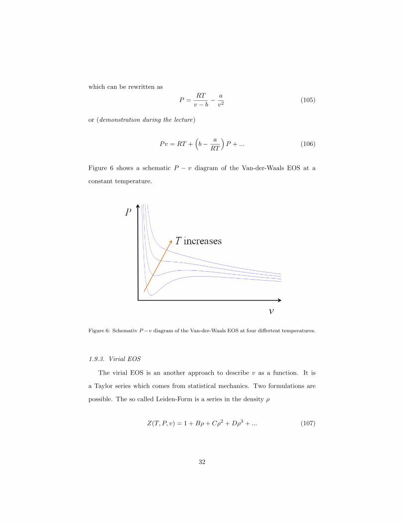
Figure 6 shows a schematic P − v diagram of the Van-der-Waals EOS at a
constant temperature.
Figure 6: Schemativ P −v diagram of the Van-der-Waals EOS at four differtent temperatures.
1.9.3. Virial EOS
The virial EOS is an another approach to describe v as a function. It is
a Taylor series which comes from statistical mechanics. Two formulations are
possible. The so called Leiden-Form is a series in the density ρ
Z(T, P, v) = 1 +Bρ+ Cρ2 +Dρ3 + ... (107)
32
The Berlin-Form uses pressure
Z(T, P, v) = 1 +B′P + C ′P 2 +D′P 3 + ... (108)
B,C,D, ... and B′, C ′, D′, ... respectively are functions of temperature. In many
cases, stopping the development of the series after the second term yields a
description that is sufficient which is
Z(T, P, v) = 1 +B′(T )P (109)
The temperature for which B′ is zero is called Boyle temperature, which indi-
cates ideal gas behavior. Please note that one can either include R (the gas
constant) into B or write it seperately leading to different expressions for B,
which is usually given as an empirical equation, finally leading to many different
formulations that can be found.
Gases can be characterized by the compressibility Z(T, P, v) = PvRT
Ideal gases: Z(T, P, v) = 1
Different EOS can be used to describe real gases.
1.10. Fugacity
In the scope of this class, the ideal gas law, the Van-der-Waals EOS, and
the virial EOS will be the only EOS considered. Rather than recalculating all
thermodynamic quantities for every EOS we will focus on the chemical potential
µ (as this is the quantity that defines equilibrium with respect to mass transfer).
We recall for an ideal gas (equation 100) for T =const.:
dTµ∗ =
RT
PdP (110)
33
For a real gas one could insert an expression for v and try to come up with an
expression for µ. A much more comfortable approach however is to replace the
pressures P and Pr in equation 110 by a new quantity called fugacity:
dTµ = RTdT ln f (111)
where the relationship between the fugacity f and pressure P is given as
limP→0
f(T, P )
P= 1 (112)
This means that for very low pressures where one reaches ideal gas behavior,
pressure and fugacity are the same. Hence, one can imagine the quantity fugac-
ity to be something like a corrected pressure (for the gas phase) to reflect real
gas properties.
Instead of looking at the integrated equations for the chemical potential we
can also look at the differential. For the ideal gas this was derived as (note that
the subscript T indicates constant temperature):
dTµ∗ = RTd lnP (113)
which is for non-ideal gases by replacing P with f
dTµ = RTd ln f (114)
Integrating from any state (or phase) α to state β yields
µα − µβ = RT lnfα
fβ(115)
34
If one wants to calculate either µα or µβ we start using the reference state r:
µα = µαr +RT lnfα
fαr(116)
µβ = µβr +RT lnfβ
fβr(117)
If we define a common reference state for the chemical potential such that
µαr = µβr and fαr = fβr (118)
the requirement for equilibrium with respect to mass transfer (µα = µβ) is only
fullfilled when
fα(T, P ) = fβ(T, P ) (119)
This is called isofugacity condition which has to be fulfilled if two phases are in
equilibrium with each other. Exploiting the fugacity for a real gas we can write
by integrating in the variable p from a reference gas pressure Pr to the actual
pressure P
1
RTdTµ = dT ln f =
v
RTdTP (120)
lnf(T, P )
f(T, Pr)=
∫ P
Pr
v
RTdp
In general
lnP
Pr=
∫ P
Pr
1
pdp (121)
Substracting the two equations yields
ln
(f(T, P )
f(T, Pr)
Pr
P
)=
∫ P
Pr
(v
RT− 1
p
)dp (122)
35
If P ∗ is chosen so small the the gas at P ∗ behaves like an ideal gas, then
f(T, P ∗) = P ∗ and the equation above simplifies to (where we now take that
P ∗ = 0 for the sake of simplicity):
lnf(T, P )
P=
∫ P
0
(Z(T, p, v)− 1)
pdp (123)
Reconsidering all three EOS that we know so far:
• Ideal Gas Law: Z(T, P, v) = 1⇒ (Z − 1) = 0⇒ f(T, P ) = P
• Virial EOS: Z(T, P, v) = 1 + BPRT
• Van-der-Waals EOS: Z(T, P, v) = 1 +(b− a
RT
)PRT ...
The fugacity f can either have values bigger or smaller than P . Three exam-
ple curves in a P − f diagram are shown in figure 7. Note that in a closed
box the pressure that you can measure directly (via a manometer) will still
be P . However, the gas inside the box will behave in terms of equilibrium
with respect to mass transfer like there was only the corrected pressure f .
The fugacity, the quantity that defines equilibrium with respect to
mass transfer, can be calculated using an EOS and the compressibility Z.
The fugacity is defined by the differential equation dTµ = RTdT ln f
subject to the boundary condition limP→0f(T,P )P = 1.
For ideal gases f(T, P ) = P . In general: f(T, P ) = P exp(∫ P
0(Z(T,p,v)−1)
p dp)
This shows that f is a corrected (or effective) pressure.
1.11. Fugacity in the Liquid Phase - Single Component Vapor Liquid Equilib-
rium (VLE)
Now that we know how to calculate the fugacity in the gas phase for ideal
and non-ideal gases, we have to find out how to calculate the fugacity in the
36
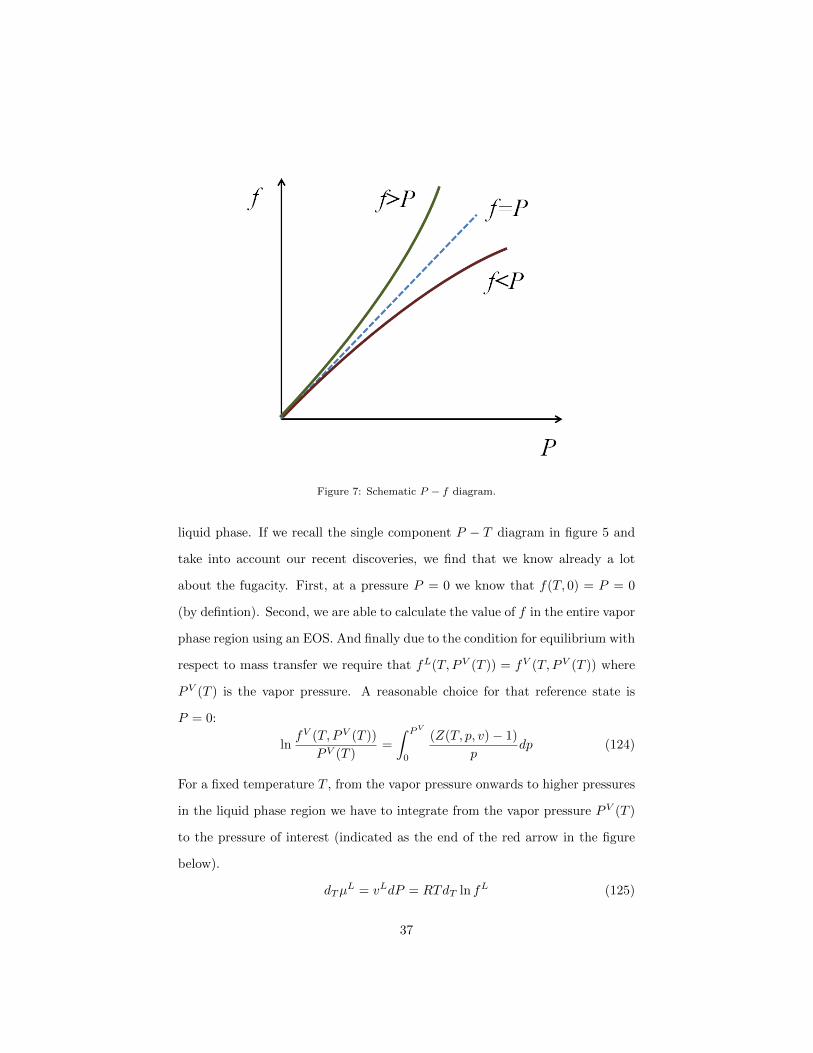
Figure 7: Schematic P − f diagram.
liquid phase. If we recall the single component P − T diagram in figure 5 and
take into account our recent discoveries, we find that we know already a lot
about the fugacity. First, at a pressure P = 0 we know that f(T, 0) = P = 0
(by defintion). Second, we are able to calculate the value of f in the entire vapor
phase region using an EOS. And finally due to the condition for equilibrium with
respect to mass transfer we require that fL(T, PV (T )) = fV (T, PV (T )) where
PV (T ) is the vapor pressure. A reasonable choice for that reference state is
P = 0:
lnfV (T, PV (T ))
PV (T )=
∫ PV
0
(Z(T, p, v)− 1)
pdp (124)
For a fixed temperature T , from the vapor pressure onwards to higher pressures
in the liquid phase region we have to integrate from the vapor pressure PV (T )
to the pressure of interest (indicated as the end of the red arrow in the figure
below).
dTµL = vLdP = RTdT ln fL (125)
37
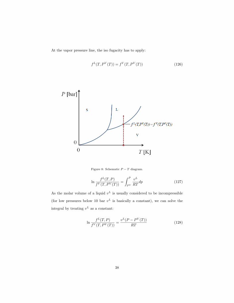
At the vapor pressure line, the iso fugacity has to apply:
fL(T, PV (T )) = fV (T, PV (T )) (126)
Figure 8: Schematic P − T diagram.
lnfL(T, P )
fV (T, PV (T ))=
∫ P
PV
vL
RTdp (127)
As the molar volume of a liquid vL is usually considered to be incompressible
(for low pressures below 10 bar vL is basically a constant), we can solve the
integral by treating vL as a constant:
lnfL(T, P )
fV (T, PV (T ))=vL(P − PV (T ))
RT(128)
38
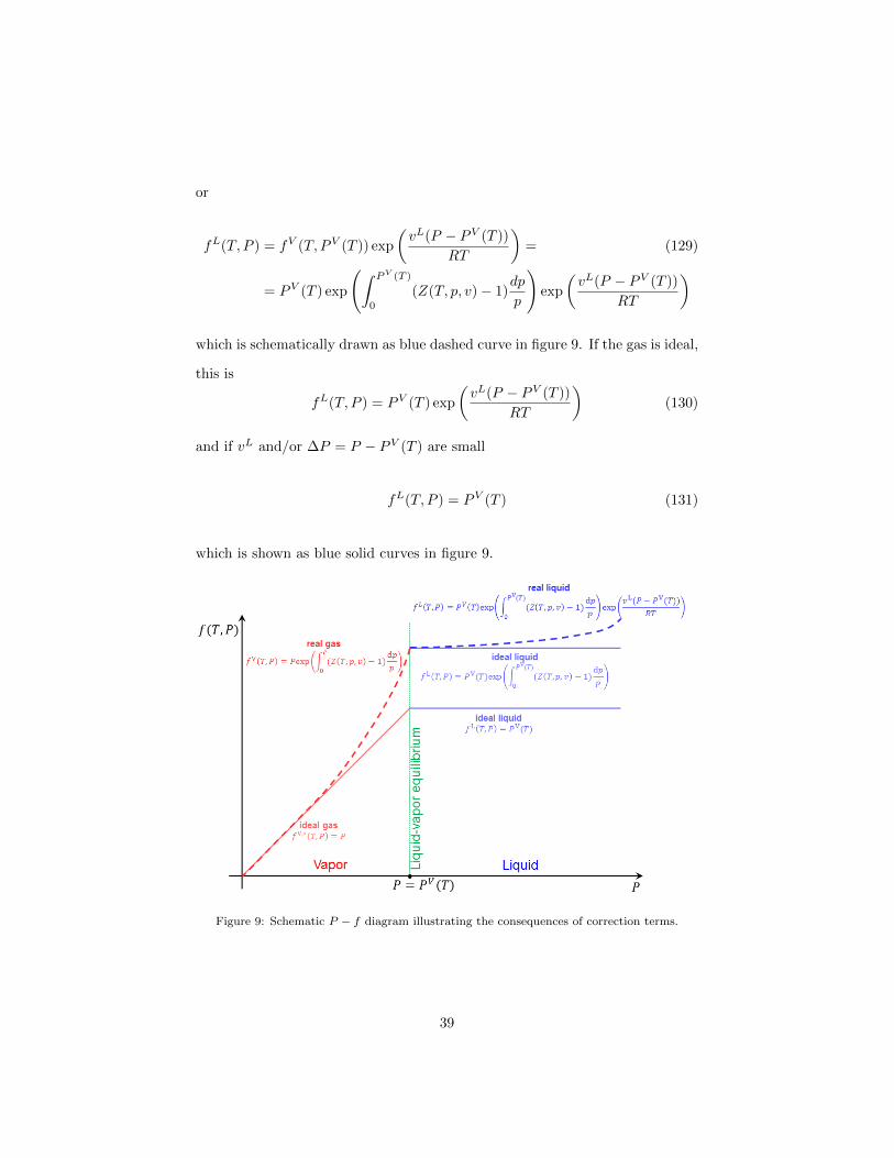
or
fL(T, P ) = fV (T, PV (T )) exp
(vL(P − PV (T ))
RT
)= (129)
= PV (T ) exp
(∫ PV (T )
0
(Z(T, p, v)− 1)dp
p
)exp
(vL(P − PV (T ))
RT
)
which is schematically drawn as blue dashed curve in figure 9. If the gas is ideal,
this is
fL(T, P ) = PV (T ) exp
(vL(P − PV (T ))
RT
)(130)
and if vL and/or ∆P = P − PV (T ) are small
fL(T, P ) = PV (T ) (131)
which is shown as blue solid curves in figure 9.
Figure 9: Schematic P − f diagram illustrating the consequences of correction terms.
39
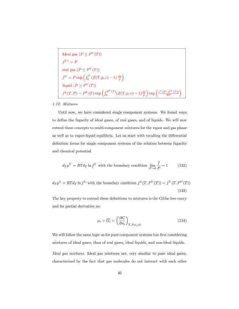
Ideal gas (P ≤ PV (T ))
fV ∗ = P
real gas (P ≤ PV (T ))
fV = P exp(∫ P
0(Z(T, p, v)− 1) dpp
)liquid (P ≥ PV (T ))
fL(T, P ) = PV (T ) exp(∫ PV (T )
0(Z(T, p, v)− 1)dpp
)exp
(vL(P−PV (T ))
RT
)1.12. Mixtures
Until now, we have considered single component systems. We found ways
to define the fugacity of ideal gases, of real gases, and of liquids. We will now
extend these concepts to multi-component mixtures for the vapor and gas phase
as well as to vapor-liquid equilibria. Let us start with recalling the differential
definition forms for single component systems of the relation between fugacity
and chemical potential.
dTµV = RTdT ln fV with the boundary condition lim
P→0
f
P= 1 (132)
dTµL = RTdT ln fL with the boundary condition fL(T, PV (T )) = fV (T, PV (T ))
(133)
The key property to extend these definitions to mixtures is the Gibbs free enery
and its partial derivative as:
µi = Gi =
(∂G
∂ni
)T,P,nj 6=i
(134)
We will follow the same logic as for pure component systems but first considering
mixtures of ideal gases, than of real gases, ideal liquids, and non-ideal liquids.
Ideal gas mixtures. Ideal gas mixtures are, very similiar to pure ideal gases,
characterized by the fact that gas molecules do not interact with each other
40
(one might say, they are not aware of the presence of other molecules and in the
case of mixtures, even of molecules of another species). So using the defintion of
the partial pressure Pi = Pyi we find that the chemical potential of an ideal gas
in a mixture is equal to the chemical potential of the same substance if it were
a pure component at the pressure equal to the partial pressure of that species
in the mixture:
µV ∗i (T, P, y)︸ ︷︷ ︸mixture
= µV ∗i (T, Pi)︸ ︷︷ ︸pure
(135)
The equation above can also be considered as a defintion of an ideal gas mixture.
If we consider a reference pressure Pr we can calculate the chemical potential of
the ideal gas in the mixture
µV ∗i (T, P, y) = µV ∗i (T, Pr) +RT lnPiPr
= (136)
= µV ∗i (T, Pr) +RT lnP
Pr+RT ln yi =
= µV ∗i (T, P ) +RT ln yi
In differential form at constant T this is:
dTµV ∗i (T, P, y) = RTdT lnPi (137)
Real gas mixtures. When we compare the above equation to equation 132 we
can recall that for a single component system we replaced the pressure with the
fugacity which acted like a corrected pressure. The same approach is now used
for mixtures of real gases:
dTµVi (T, P, y) = RTdT ln fi(T, P, y) (138)
41
The boundary condition changes accordingly to
limP→0
fi(T, P, y)
Pi= 1 (139)
Using this defintion, we see that for an ideal gas f∗i (T, P, y) = Pyi. For a real
gas, an equation of state that takes into account interactions between molecules
of different gas species would be needed. One can obtain such EOS and different
approaches exist in literature. However in the scope of our lecture, we will limit
ourselves to ideal gas mixtures as there is no academic benefit from extending
our findings in such a way. Instead, we want to determine the chemical potential
in liquid mixtures.
Ideal liquid mixtures. First we need to define an ideal liquid mixture (note
that we use 0 to indicate ideal behavior). An ideal mixture is characterized
by ∆Vmix = 0. We will investigate the meaning of this property in the next
but one chapter. In ideal mixtures, molecules in this mixture do not interact
with each other (one might formulate that molecules of different species are not
aware of the presence of another species). So similar to equation 136:
µ0i (T, P, x)︸ ︷︷ ︸mixture
= µi(T, P )︸ ︷︷ ︸pure
+RT lnxi (140)
Expressing this equation via the fugacity in the same manner as demonstrated
for the gas phase yields
fL0i (T, P, x)︸ ︷︷ ︸mixture
= fLi (T, P )︸ ︷︷ ︸pure
xi (141)
Non-ideal liquid mixtures. Many real liquid mixtures however do not behave
ideal. For non-ideal liquid mixtures of multiple components, we introduce a
new correction term which we call activity coefficient γi = γi(T, P, x), such that
42
fLi (T, P, x) = fL0i (T, P, x)γi(T, P, x) = fLi (T, P )xiγi(T, P, x) (142)
In this way, the fugacity of a component i = 1, 2, ..., C in a mixture is equal to
the product of the fugacity of the pure component at T and P multiplied with
the molar fraction xi and the activity coefficient (which itself is a function of
temperature T , pressure P , and composition x). The activity coefficient for an
ideal liquid is 1, which reduces equation 142 to equation 141.
In order to calculate the fugacity of the non-ideal liquid phase, an expression
for this correction term is needed. We consider the difference between an ideal
and a non-ideal liquid mixture. In general, this can be done by splitting a ther-
modynamic quantity into one term that accounts for the ideal mixing behavior
and one term for the excess of that quantity (indicated by E). For the Gibbs
free energy this is:
G(T, P, n) = G0(T, P, n) +GE(T, P, n) (143)
Excess of the Gibbs free energy. It seems that information on the non-ideal
behavior of a mixture can be obtained from investigation the excess Gibbs free
energy. We recall equation 114
dTµi = RTdT ln fi (144)
The difference between the ideal liquid to the real liquid yields:
µLi (T, P, x)− µL0i (T, P, x) = RT lnfLi (T, P, x)
fL0i (T, P, x)= (145)
= RT ln γi(T, P, x) = Gi −G0
i =
=
(∂(G−G0)
∂ni
)T,P,nj 6=i
=
(∂(ngE)
∂ni
)T,P,nj 6=i
43
gE (the molar excess gibbs free energy) is a quantity that describes how well
two liquids mix. If it were 0, there would be no interaction between molecules
of different species and the liquid would behave ideal. If it is bigger than 0,
repulsive forces are present. If it is smaller than 0, attractive forces are present.
Many models exist to describe gE and hence γi as a function of temperature,
pressure, and composition. For a binary mixture with C = 2, gE can be de-
scribed for example by an empirical equation that uses a constant A where x1
and x2 are the mole fractions of the two components of the binary mixture:
gE
RT= Ax1x2 (146)
Different values of A result in different values for gE in the range between
attractive and repulsive forces in the liquid mixture. Figure 10 shows possible
behaviors. On the x-axis you find the composition so that at the left x1 = 0
and x2 = 1 and at the right x1 = 1 and x2 = 0 respectively. The y-axis is gE .
Inserting equation 146 into equation 145 yields
ln γi =1
RT
(∂ngE
∂ni
)T,P,nj 6=i
(147)
ngE
RT=An2x1x2
n= A
n1n2n1 + n2
(148)
⇒ ln γi = A(1− xi)2 (149)
which is called Porter equation.
44
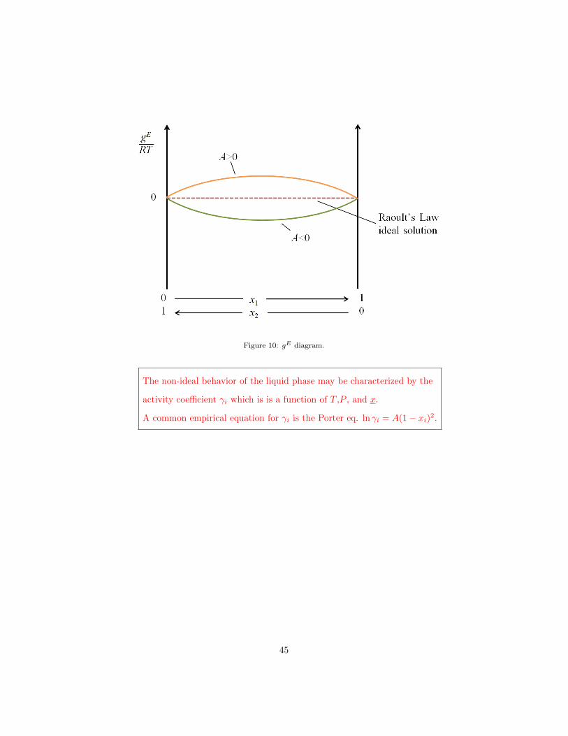
Figure 10: gE diagram.
The non-ideal behavior of the liquid phase may be characterized by the
activity coefficient γi which is is a function of T ,P , and x.
A common empirical equation for γi is the Porter eq. ln γi = A(1− xi)2.
45
1.12.1. Vapor Liquid Equilibrium for mixtures
The condition for phase equilibrium (iso-fugacity condition) for single com-
ponent systens (equation 119) is extended for mixtures to:
µαi = µβi ⇔ fαi = fβi (150)
So the iso-fugacity condition has to be fulfilled for every species i. For a vapor
liquid equilibrium this reads as:
fVi (T, P, y) = fLi (T, P, x) (151)
In the scope of this lecture, we will only use the two iso-fugacity conditions as
shown in table 1.12.1, i.e. we will focus on an ideal gas phase (as mentioned
above).
Table 1: Iso-fugacity conditions for mixtures.
vapor phase liquid phase
ideal Pyi = PVi (T )xi ideal
ideal Pyi = PVi (T )xiγi(T, P, x) non-ideal
In the case of an ideal gas and an ideal solution, the equation iso-fugacity
condition can be written as
Pyi = PVi (T )xi (152)
which is also known as Raoult’s Law and is the simplest expression for vapor-
liquid equilibrium.
VLE for a mixture is defined by the isofugacity condition:
fVi (T, P, y) = fLi (T, P, x). (Table 1)
46
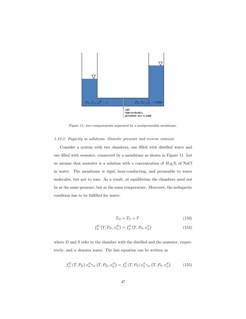
Figure 11: two compartments separated by a semipermeable membrane.
1.12.2. Fugacity in solutions: Osmotic pressure and reverse osmosis
Consider a system with two chambers, one filled with distilled water and
one filled with seawater, connected by a membrane as shown in Figure 11. Let
us assume that seawater is a solution with a concentration of 35 g/L of NaCl
in water. The membrane is rigid, heat-conducting, and permeable to water
molecules, but not to ions. As a result, at equilibrium the chambers need not
be at the same pressure, but at the same temperature. Moreover, the isofugacity
condition has to be fulfilled for water:
TD = TS = T (153)
fDw(T, PD, x
Dw
)= fSw
(T, PS , x
Sw
)(154)
where D and S refer to the chamber with the distilled and the seawater, respec-
tively; and w denotes water. The last equation can be written as
fDw (T, PD)xDwγw(T, PD, x
Dw
)= fSw (T, PS)xSwγw
(T, PS , x
Sw
)(155)
47
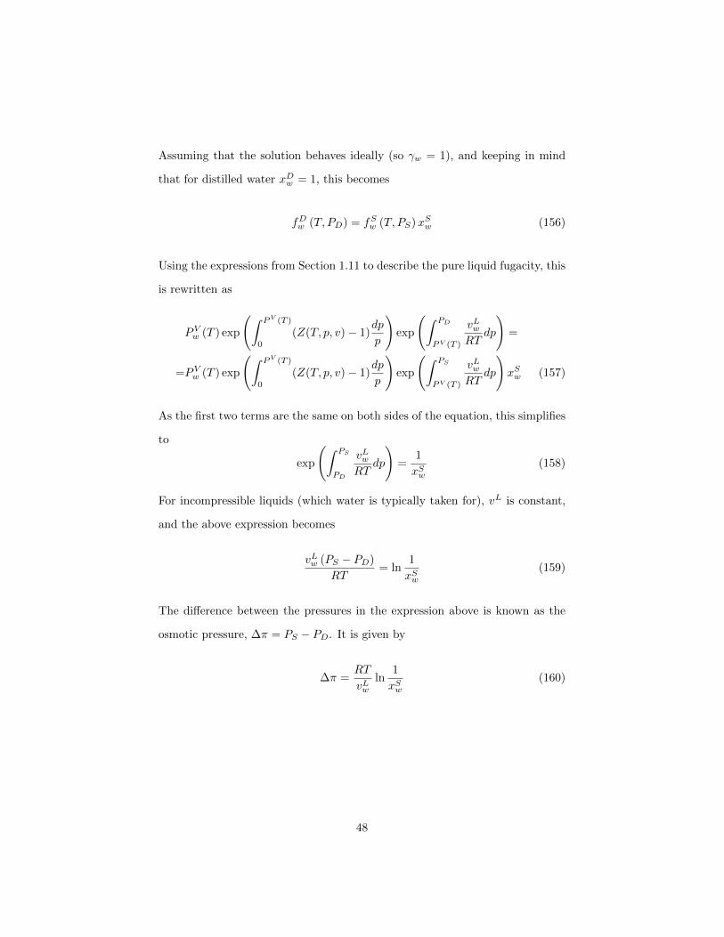
Assuming that the solution behaves ideally (so γw = 1), and keeping in mind
that for distilled water xDw = 1, this becomes
fDw (T, PD) = fSw (T, PS)xSw (156)
Using the expressions from Section 1.11 to describe the pure liquid fugacity, this
is rewritten as
PVw (T ) exp
(∫ PV (T )
0
(Z(T, p, v)− 1)dp
p
)exp
(∫ PD
PV (T )
vLwRT
dp
)=
=PVw (T ) exp
(∫ PV (T )
0
(Z(T, p, v)− 1)dp
p
)exp
(∫ PS
PV (T )
vLwRT
dp
)xSw (157)
As the first two terms are the same on both sides of the equation, this simplifies
to
exp
(∫ PS
PD
vLwRT
dp
)=
1
xSw(158)
For incompressible liquids (which water is typically taken for), vL is constant,
and the above expression becomes
vLw (PS − PD)
RT= ln
1
xSw(159)
The difference between the pressures in the expression above is known as the
osmotic pressure, ∆π = PS − PD. It is given by
∆π =RT
vLwln
1
xSw(160)
48
For dilute systems (i.e. xSw ≈ 1), a linear approximation can be used for the
logarithm, resulting in
∆π =RT
vLw
(1− xSw
)= RTc (161)
where c is the concentration of ions in solution. The seawater considered in
this example has a NaCl concentration of 35 g/L, and after dissolution an ion
concentration of 1198 mol/m3 (Na+ + Cl− ions). Using the expression above
one obtains ∆π = 2.9 MPa for a temperature of 20 ◦C. This is the pressure to
be applied to a solution to prevent its dilution with pure water flowing into the
solution through a semi-permeable membrane. If on the other hand, additional
pressure is applied to the solution such that
PS > PD + ∆π (162)
then fSw > fDw , and pure water flows from the seawater compartment to the
pure water compartment; a technique commonly used in seawater desalination.
49
1.12.3. Volume of a mixture
You might remember a high school experiment where one pours together 50
mL water and 50 mL ethanol. The total volume of that mixture is 97 mL instead
of 100 mL as one might expect. This property of mixing is closely related to
what we derived in the previous chapter.
Imagine C barrels that are filled with ni number of moles of species i each as
shown in figure 12 so that each barrel only contains molecules of one pure species
i each. The initial total volume of all liquids in all small barrels is the sum of
the products of the molar volumes and the number of moles in all barrels. The
molar volume is the derivative of the chemical potential with respect to pressure
of the pure species i.
Vinitial =
C∑i=1
niνLi =
C∑i=1
ni
(∂µi∂P
)T
=
C∑i=1
niRT
(∂ ln fLi (T, P )
∂P
)T
(163)
The final volume after mixing is the sum of the product of the number of moles
of species i and the corresponding molar volume in the mixture Vi.
Vfinal =
C∑i=1
niV i =
C∑i=1
ni
(∂µLi∂P
)T,n
= RT
C∑i=1
ni
(∂ ln fLi (T, P, x)
∂P
)T,n
(164)
= RT
C∑i=1
ni∂
∂P
(ln fLi (T, P ) + lnxi + ln γi(T, P, x)
)T,n
=
=
C∑i=1
niνLi +RT
C∑i=1
(∂ ln γi∂P
)T,n
The difference between the total volume before and after mixing is ∆Vmix:
∆Vmix = Vfinal − Vinitial = RT
C∑i=1
ni
(∂ ln γi∂P
)T,x
(165)
For an ideal solution, the activity coefficient is γ = 1 and hence ∆Vmix = 0.
50
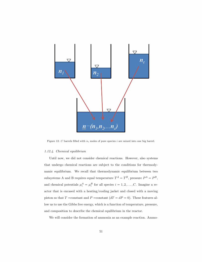
Figure 12: C barrels filled with ni moles of pure species i are mixed into one big barrel.
1.12.4. Chemical equilibrium
Until now, we did not consider chemical reactions. However, also systems
that undergo chemical reactions are subject to the conditions for thermody-
namic equilibrium. We recall that thermodynamic equilibrium between two
subsystems A and B requires equal temperature TA = TB , pressure PA = PB ,
and chemical potentials µAi = µBi for all species i = 1, 2, . . . , C. Imagine a re-
actor that is encased with a heating/cooling jacket and closed with a moving
piston so that T =constant and P =constant (dT = dP = 0). These features al-
low us to use the Gibbs free energy, which is a function of temperature, pressure,
and composition to describe the chemical equilibrium in the reactor.
We will consider the formation of ammonia as an example reaction. Ammo-
51
nia NH3 is formed from hydrogen H2 and nitrogen N2 as
1N2 + 3H2 2NH3 (166)
or
0 = 2NH3 − 1N2 − 3H2 (167)
In general, a chemical reaction will be written as:
C∑i=1
νiAi = 0 (168)
where Ai represents species i, and νi is its stoichiometric coefficient, i.e. positive
for products and negative for reactants. Table 2 illustrates its meaning (compare
to equation 166). Two remarks are worth noting. First, note that the last
equation enforces fulfillment of atmoic balance, i.e. atoms are neither created
nor destroyed in a chemical reaction. Second, the last equation is formulated in
s slightly different manner than in the script of Thermo II, Prof. Boulouchos.
In this lecture we use equation 168.
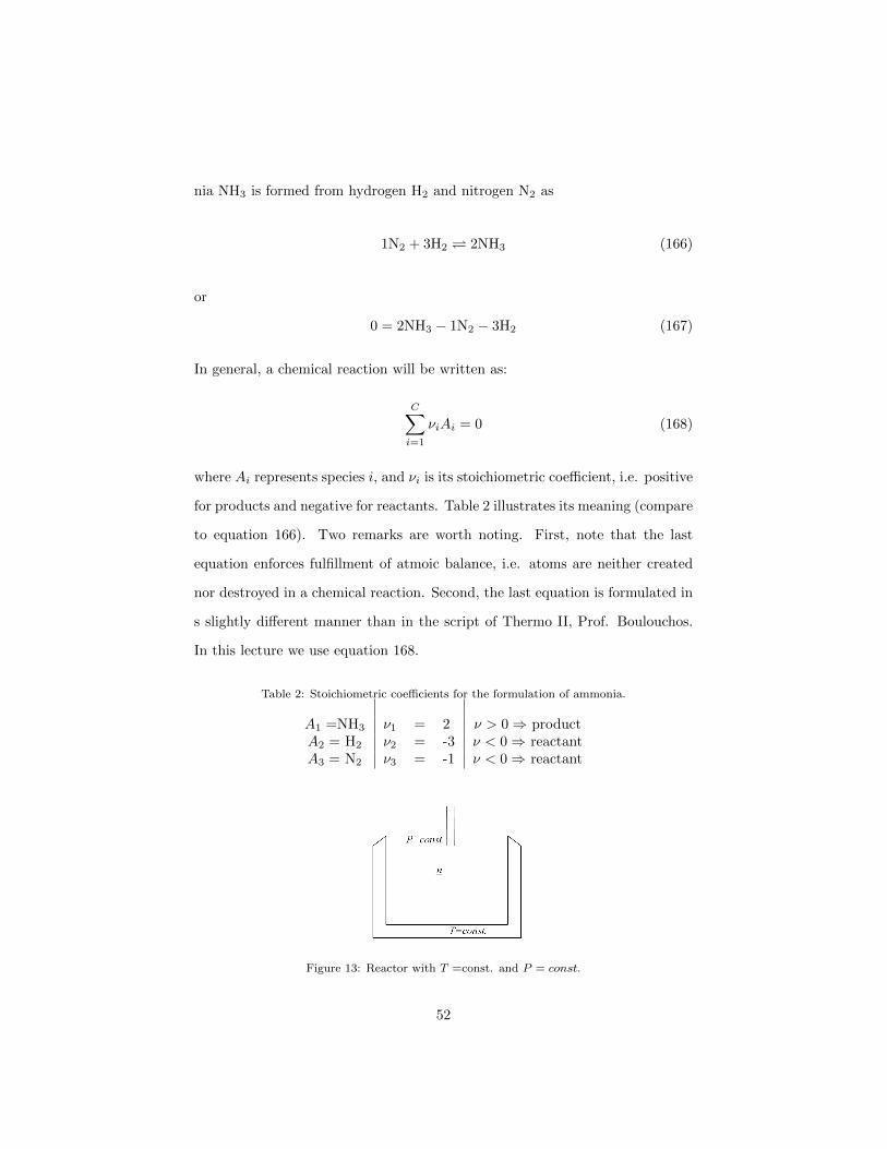
Table 2: Stoichiometric coefficients for the formulation of ammonia.
A1 =NH3 ν1 = 2 ν > 0⇒ productA2 = H2 ν2 = -3 ν < 0⇒ reactantA3 = N2 ν3 = -1 ν < 0⇒ reactant
Figure 13: Reactor with T =const. and P = const.
52
In a closed reactor conservation of mass applies. Let us consider a mixture of
products and reactants that are initially present in amounts n0i (i = 1, . . . , C).
Let us also assume that the reaction defined by equation 166 has proceeded, and
let us call the extent of the reaction (number of moles reacted) as λ. Therefore,
the number of moles of species i can be written as:
ni = n0i + ∆ni = n0i + νiλ (169)
where ∆ni is the number of moles that have been formed or consumed during
the reaction, which is equal to the product of the stoichiometric coefficient νi
and λ. The differential form of the above equation is:
dni = νidλ (170)
The differential of the Gibbs free energy is:
dG = −SdT + V dP +
C∑i=1
µidni (171)
At T, P constant (dP = dT = 0) the equation above reduces to
dG =
C∑i=1
µidni (172)
Using equation 170 yields
dG =
(C∑i=1
µiνi
)dλ (173)
in chemical equilibrium, G is minimal and dG = 0. Hence:
C∑i=1
µiνi = 0 (174)
53
In the special case of an ideal gas phase, the chemical potential in the mixture
is:
µ∗i (T, P, y) = µ∗i (T, Pr) +RT lnPiPr
(175)
combining the last two equations we find
dG
dλ=
C∑i=1
νiµ∗i (T, P, y) =
C∑i=1
νiµ∗i (T, Pr) +RT
C∑i=1
νi lnPiPr
(176)
One defines the Gibbs free energy of a reaction ∆G0r as
∆G0r (T, Pr) =
C∑i=1
νiµ∗i (T, Pr) (177)
The sum of the logarithms can be expressed as a product so that
dG
dλ=
C∑i=1
νiµ∗i (T, P, y) = ∆G0
r (T, Pr) +RT ln
C∏i=1
(PyiPr
)νi= (178)
= ∆G0r (T, Pr) +RT ln
((P
Pr
)ν C∏i=1
yνii
)=
= RT
[∆G0
r (T, Pr)
RT+ ln
((P
Pr
)ν C∏i=1
yνii
)]
where ν =∑Ci=1 νi. At equilibrium dG = 0, hence
exp−∆G0
R(T )
RT︸ ︷︷ ︸Keq(T )
=
(P
Pr
)ν C∏i=1
yνii (179)
Keq(T ) is called equilibrium constant and is a function of temperature. Note
that the right hand side of the equation is often called Q, which is a function of
T ,P ,y.
dG
dλ= −RT lnKeq(T ) +RT lnQ(T, P, y) (180)
54
Two important calculations based on these findings can be performed. The
first application is to calculate the equilibrium composition in a closed reactor
by coupling equation 179 with equation 169. In this manner, the molar fraction
of species i becomes a function of the extent of the reaction λ:
yi =ni∑Cj=1 nj
=n0i + νiλ∑C
j=1 n0j + λ
∑Cj=1 νj
= yi(λ) (181)
For a given temperature T and pressure P , the extent of the reaction in equi-
librium and hence the equilibrium composition can be obtained.
The second application is to find out about the direction of the evolution of
a reaction if it is a spontaneous process
0 > dG =
(C∑i=1
νiµi
)dλ (182)
that proceeds towards reaching equilibrium (dG = 0). Using equation 180 we
may write:
C∑i=1
νiµi = ∆G0r +RT lnQ = −RT lnKeq +RT lnQ = RT ln
Q
Keq≶ 0 (183)
If Q > Keq ⇒ dλ < 0, the reaction proceeds backwards (products→ reactants).
If Q < Keq ⇒ dλ > 0, the reaction proceeds forwards (reactants → products).
If Q = Keq ⇒ dλ = 0, the reaction is in equilibrium.
Returning to the ammonia formation example where ν = −2 we find that
equation 179 is:
Keq(T ) =
(P
Pr
)−2 y2NH3
yN2y3H2
(184)
Note that a common procedure is to take Pr = 1 bar.
55
1.13. Liquid vapor equilibrium in binary mixtures
While the iso-fugacity condition that we used in previous chapters is valid
also for high numbers of components, in the scope of this chapter we will focus
on binary systems (C = 2⇒ i = 1, 2) and we consider situations when there can
be equilibrium between a liquid and a vapor phase. Equilibrium with respect
to mass transfer for these systems (LVE) is characterized by the iso-fugacity
condition
fVi (T, P, y1, y2) = fLi (T, P, x1, x2) i = 1, 2 (185)
where we have implicitly enforced the condition for thermal and mechanical
equilibrium, i.e. same T and P in the two phases. Note that for C = 2,
x2 = 1−x1 and y2 = 1−y1. We assume that component 1 is more volatile than
component 2.
1.13.1. LVE in single component systems
Each component has its own phase diagram (schematically drawn in Figure
14 for components 1 and 2). LVE is given by the boiling curve which can be
calculated with the Antoine equation (equation 92). At temperature T we find
PV1 (T ) and PV2 (T ), with PV1 (T ) > PV2 (T ) because of our choice that component
1 is more volatile than component 2. At P = 1 bar, we have the boiling points
T b1 and T b2 , with T b1 < T b2 again because 1 is more volatile than 2. At a fixed
pressure P a single component evaporates at constant temperature, i.e. the
temperature on the LVE curve of the phase diagram corresponding to P . We
want to investigate liquid vapor equilibrium in binary mixtures for which we
will develop suitable diagrams.
1.13.2. P-xy diagrams
The first type of diagram that we want to consider is the P − xy diagram
where the temperature is kept constant. With reference to figure 14, at a fixed
56
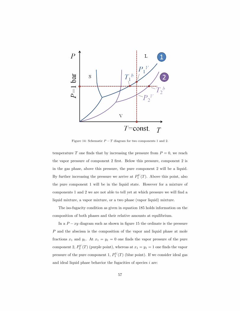
Figure 14: Schematic P − T diagram for two components 1 and 2.
temperature T one finds that by increasing the pressure from P = 0, we reach
the vapor pressure of component 2 first. Below this pressure, component 2 is
in the gas phase, above this pressure, the pure component 2 will be a liquid.
By further increasing the pressure we arrive at PV1 (T ). Above this point, also
the pure component 1 will be in the liquid state. However for a mixture of
components 1 and 2 we are not able to tell yet at which pressure we will find a
liquid mixture, a vapor mixture, or a two phase (vapor liquid) mixture.
The iso-fugacity condition as given in equation 185 holds information on the
composition of both phases and their relative amounts at equilibrium.
In a P − xy diagram such as shown in figure 15 the ordinate is the pressure
P and the abscissa is the composition of the vapor and liquid phase at mole
fractions x1 and y1. At x1 = y1 = 0 one finds the vapor pressure of the pure
component 2, PV2 (T ) (purple point), whereas at x1 = y1 = 1 one finds the vapor
pressure of the pure component 1, PV1 (T ) (blue point). If we consider ideal gas
and ideal liquid phase behavior the fugacities of species i are:
57
fV ∗i = Pyi = Pi (186)
fL0i = PVi (T )xi
LVE is given by the iso-fugacity conditions
P1 = PV1 (T )x1 (187)
P2 = PV2 (T )x2
Plotting the partial pressure of each of the two components, which is given
by the fugacity in the liquid phase, yields the blue (component 1) and purple
(component 2) lines in figure 15. The sum of the partial pressures is the total
pressure of the system:
P = P1 + P2 = PV1 (T )x1 + PV2 (T )x2 (188)
which is drawn in orange in figure 15. This curve is commonly called bubble
point curve.
The vapor mole fraction y1 that is in equilibrium with a given liquid mole
fraction x1 at the system pressure P is:
y1 =P1
P=
fL1fL1 + fL2
=PV1 (T )x1
PV1 (T )x1 + PV2 (T )x2(189)
It is used to draw the dew point curve (green curve in figure 15), i.e. the curve
that represents the vapor phase mole fraction in equilibrium with the liquid
phase mole fraction at the pressure P . In other words the liquid and vapor
phases at equilibrium correspond to the points on the orange and green curves,
respectively.
58
For a non-ideal liquid mixture the construction is almost identical. The
liquid phase fugacity in the non-ideal case is described by correcting the ideal
liquid fugacity with the activity coefficient γi as
fLi = PVi (T )xiγi(T, P, x1, x2) (190)
Please recall that γi can either be bigger or smaller than 1 which leads to a
bended curve as compared to the straight line of the ideal case (γi = 1, drawn
as dashed blue line for component 1 into figure 16 and dashed purple line for
component 2 into figure 16). If γi is bigger than 1, the resulting curve will be
above the ideal case straight line (this is drawn as solid blue (component 1)
and solid purple (component 2) curves into figure 16), if γi is smaller than 1
the resulting curve will be below the straight line of the ideal case. The total
system pressure curve which is drawn in solid orange in figure 16 is given by
P = P1 + P2 = PV1 (T )x1γ1(T, P, x1, x2) + PV2 (T )x2γ2(T, P, x1, x2) (191)
which is a bended curve that is above the straight line of the ideal case (ideal:
dashed orange curve in figure 16) for γi > 1 and below the straight line of the
ideal case if γi < 1.
The green curve in figure 16, i.e. the dew point curve, is obtained similar
to the ideal liquid case and is indicating the vapor composition y1 that is in
equilibrium with a given liquid composition x1 at pressure P :
y1 =P1
P=
fL1fL1 + fL2
=PV1 (T )x1γ1(T, P, x1, x2)
PV1 (T )x1γ1(T, P, x1, x2) + PV2 (T )x2γ2(T, P, x1, x2)
(192)
You can use the code that you prepared for the home assignment 5.1 to visualize
different values of γi by changing the value of A of the porter equation.
59
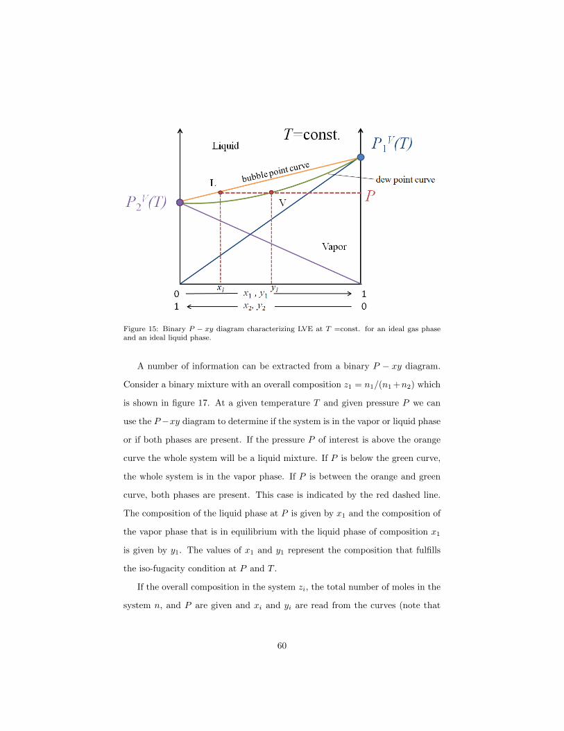
Figure 15: Binary P − xy diagram characterizing LVE at T =const. for an ideal gas phaseand an ideal liquid phase.
A number of information can be extracted from a binary P − xy diagram.
Consider a binary mixture with an overall composition z1 = n1/(n1 +n2) which
is shown in figure 17. At a given temperature T and given pressure P we can
use the P−xy diagram to determine if the system is in the vapor or liquid phase
or if both phases are present. If the pressure P of interest is above the orange
curve the whole system will be a liquid mixture. If P is below the green curve,
the whole system is in the vapor phase. If P is between the orange and green
curve, both phases are present. This case is indicated by the red dashed line.
The composition of the liquid phase at P is given by x1 and the composition of
the vapor phase that is in equilibrium with the liquid phase of composition x1
is given by y1. The values of x1 and y1 represent the composition that fulfills
the iso-fugacity condition at P and T .
If the overall composition in the system zi, the total number of moles in the
system n, and P are given and xi and yi are read from the curves (note that
60
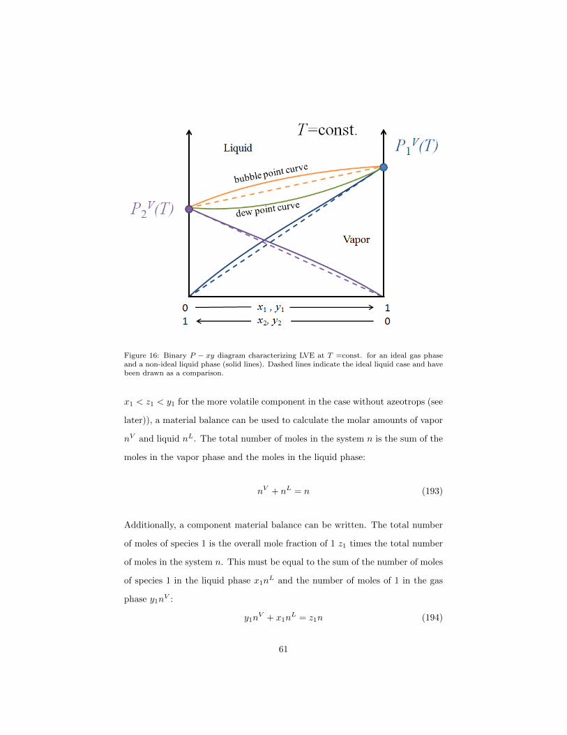
Figure 16: Binary P − xy diagram characterizing LVE at T =const. for an ideal gas phaseand a non-ideal liquid phase (solid lines). Dashed lines indicate the ideal liquid case and havebeen drawn as a comparison.
x1 < z1 < y1 for the more volatile component in the case without azeotrops (see
later)), a material balance can be used to calculate the molar amounts of vapor
nV and liquid nL. The total number of moles in the system n is the sum of the
moles in the vapor phase and the moles in the liquid phase:
nV + nL = n (193)
Additionally, a component material balance can be written. The total number
of moles of species 1 is the overall mole fraction of 1 z1 times the total number
of moles in the system n. This must be equal to the sum of the number of moles
of species 1 in the liquid phase x1nL and the number of moles of 1 in the gas
phase y1nV :
y1nV + x1n
L = z1n (194)
61
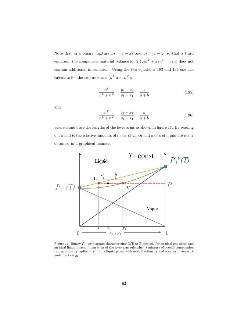
Note that in a binary mixture x2 = 1 − x1 and y2 = 1 − y1 so that a third
equation, the component material balance for 2 (y2nV + x2n
L = z2n) does not
contain additional information. Using the two equations 193 and 194 one can
calculate for the two unkowns (nL and nV ):
nL
nL + nV=y1 − z1y1 − x1
=b
a+ b(195)
and
nV
nL + nV=z1 − x1y1 − x1
=a
a+ b(196)
where a and b are the lengths of the lever arms as shown in figure 17. By reading
out a and b, the relative amounts of moles of vapor and moles of liquid are easily
obtained in a graphical manner.
Figure 17: Binary P −xy diagram characterizing LVE at T =const. for an ideal gas phase andan ideal liquid phase. Illustration of the lever arm rule when a mixture of overall compoistion(z1, z2 = 1− z1) splits at P into a liquid phase with mole fraction x1 and a vapor phase withmole fraction y1.
62
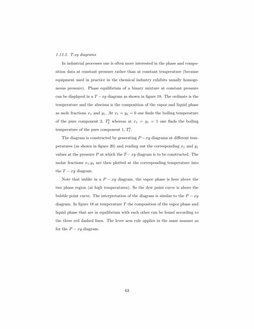
1.13.3. T-xy diagrams
In industrial processes one is often more interested in the phase and compo-
sition data at constant pressure rather than at constant temperature (because
equipment used in practice in the chemical industry exhibits usually homoge-
neous pressure). Phase equilibrium of a binary mixture at constant pressure
can be displayed in a T −xy diagram as shown in figure 18. The ordinate is the
temperature and the abscissa is the composition of the vapor and liquid phase
as mole fractions x1 and y1. At x1 = y1 = 0 one finds the boiling temperature
of the pure component 2, T b2 whereas at x1 = y1 = 1 one finds the boiling
temperature of the pure component 1, T b1 .
The diagram is constructed by generating P −xy diagrams at different tem-
peratures (as shown in figure 20) and reading out the corresponding x1 and y1
values at the pressure P at which the T −xy diagram is to be constructed. The
molar fractions x1,y1 are then plotted at the corresponding temperature into
the T − xy diagram.
Note that unlike in a P − xy diagram, the vapor phase is here above the
two phase region (at high temperatures). So the dew point curve is above the
bubble point curve. The interpretation of the diagram is similar to the P − xy
diagram. In figure 18 at temperature T the composition of the vapor phase and
liquid phase that are in equilibrium with each other can be found according to
the three red dashed lines. The lever arm rule applies in the same manner as
for the P − xy diagram.
63
Figure 18: Binary T − xy diagram characterizing LVE at P =const. for an ideal gas phaseand an ideal liquid phase.
1.13.4. x-y diagrams
Another way of representing T − xy data is by plotting the pairs of x1 and
y1 which have already been used to construct the T − xy diagram against each
other directly so that x1 is plotted on the abscissa and y1 is plotted on the
ordinate. The diagonal is x1 = y1 and is usually plotted as a visual guide. For
a given liquid composition x1 one immediately finds the composition y1 that
corresponds to the equilibrium composition of the vapor phase at the pressure
of the diagram. Note that the temperature, according to the T − xy data,
changes along the green equilibrium curve, namely it increases in the direction
of the arrow in figure 19.
64
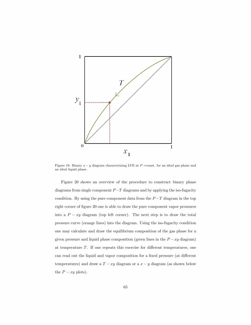
Figure 19: Binary x− y diagram characterizing LVE at P =const. for an ideal gas phase andan ideal liquid phase.
Figure 20 shows an overview of the procedure to construct binary phase
diagrams from single component P−T diagrams and by applying the iso-fugacity
condition. By using the pure component data from the P−T diagram in the top
right corner of figure 20 one is able to draw the pure component vapor pressures
into a P − xy diagram (top left corner). The next step is to draw the total
pressure curve (orange lines) into the diagram. Using the iso-fugacity condition
one may calculate and draw the equilibrium composition of the gas phase for a
given pressure and liquid phase composition (green lines in the P −xy diagram)
at temperature T . If one repeats this exercise for different temperatures, one
can read out the liquid and vapor composition for a fixed pressure (at different
temperatures) and draw a T − xy diagram or a x− y diagram (as shown below
the P − xy plots).
65
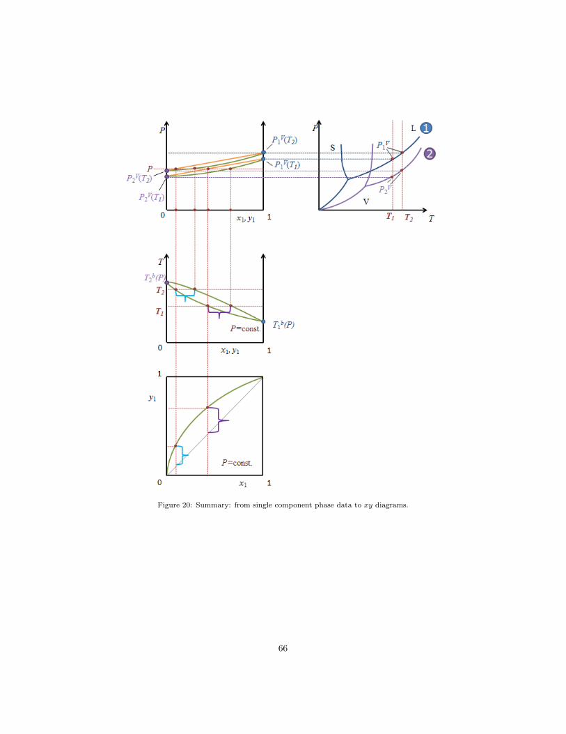
Figure 20: Summary: from single component phase data to xy diagrams.
66
1.13.5. H-xy diagrams
The last type of diagram that we want to discuss is the enthalpy-composition
diagram which is very useful for the design of the separation unit in the next
chapter. On the abscissa one finds again the composition plotted in the same
manner as in the T − xy and P − xy diagrams. On the ordinate one plots
the specific enthalpy h. The diagram is based on the T − xy diagram from
the previous chapter (so P =const.), i.e. one plots the specific enthalpy of
a liquid mixture hL(Tbp(x1), P, x1, x2) at the same temperature Tbp(x1) and
composition x1 as given by the bubble point curve (see figure 18) and the specific
enthalpy of a vapor mixture hV (Tdp, P, y1, y2) at the same temperature Tdp(y1)
and composition y1 as given by the dew point curve (see figure 18). If one
considers an ideal vapor phase, the enthalpy of species i is:
hVi (T, P ) = h∗i (Tr) +
∫ T
Tr
c∗p,idT (197)
where h∗i (Tr) is the enthalpy of an ideal gas at a reference temperature Tr and
c∗p,i is the heat capacity of an ideal gas (i.e. for a monatomic gas c∗p,i = 52R or
for a diatomic gas c∗p,i = 72R)). If one neglects the enthalpy of mixing and treats
the vapor phase as ideal, the enthalpy of the vapor phase along the dew point
curve at temperature Tdp(y1) and at the corresponding vapor phase composition
y1 is:
hV (Tdp(y1), P, y1, y2) = y1hV1 (Tdp(y1), P ) + y2h
V2 (Tdp(y1), P ) (198)
The specific liquid phase enthalpy of component i is:
hLi (T, P ) = h∗i (Tr) +
∫ T bi
Tr
c∗p,idT −∆hLVi (T bi ) +
∫ T
T bi
cLp,idT (199)
67
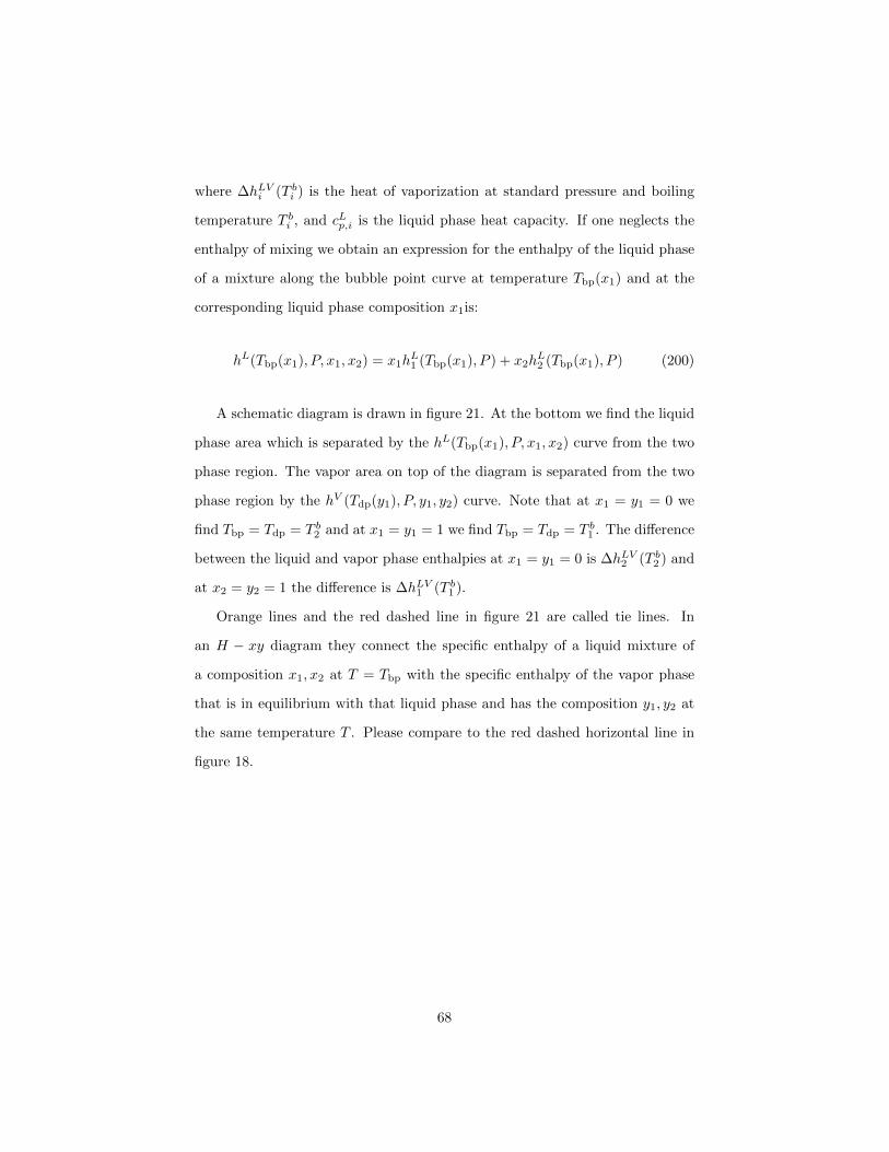
where ∆hLVi (T bi ) is the heat of vaporization at standard pressure and boiling
temperature T bi , and cLp,i is the liquid phase heat capacity. If one neglects the
enthalpy of mixing we obtain an expression for the enthalpy of the liquid phase
of a mixture along the bubble point curve at temperature Tbp(x1) and at the
corresponding liquid phase composition x1is:
hL(Tbp(x1), P, x1, x2) = x1hL1 (Tbp(x1), P ) + x2h
L2 (Tbp(x1), P ) (200)
A schematic diagram is drawn in figure 21. At the bottom we find the liquid
phase area which is separated by the hL(Tbp(x1), P, x1, x2) curve from the two
phase region. The vapor area on top of the diagram is separated from the two
phase region by the hV (Tdp(y1), P, y1, y2) curve. Note that at x1 = y1 = 0 we
find Tbp = Tdp = T b2 and at x1 = y1 = 1 we find Tbp = Tdp = T b1 . The difference
between the liquid and vapor phase enthalpies at x1 = y1 = 0 is ∆hLV2 (T b2 ) and
at x2 = y2 = 1 the difference is ∆hLV1 (T b1 ).
Orange lines and the red dashed line in figure 21 are called tie lines. In
an H − xy diagram they connect the specific enthalpy of a liquid mixture of
a composition x1, x2 at T = Tbp with the specific enthalpy of the vapor phase
that is in equilibrium with that liquid phase and has the composition y1, y2 at
the same temperature T . Please compare to the red dashed horizontal line in
figure 18.
68
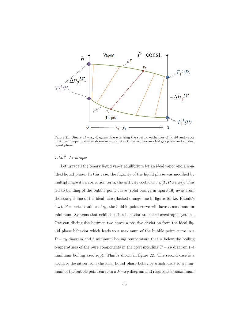
Figure 21: Binary H − xy diagram characterizing the specific enthalpies of liquid and vapormixtures in equilibrium as shown in figure 18 at P =const. for an ideal gas phase and an idealliquid phase.
1.13.6. Azeotropes
Let us recall the binary liquid vapor equilibrium for an ideal vapor and a non-
ideal liquid phase. In this case, the fugacity of the liquid phase was modified by
multiplying with a correction term, the acitivity coefficient γi(T, P, x1, x2). This
led to bending of the bubble point curve (solid orange in figure 16) away from
the straight line of the ideal case (dashed orange line in figure 16, i.e. Raoult’s
law). For certain values of γi, the bubble point curve will have a maximum or
minimum. Systems that exhibit such a behavior are called azeotropic systems.
One can distinguish between two cases, a positive deviation from the ideal liq-
uid phase behavior which leads to a maximum of the bubble point curve in a
P − xy diagram and a minimum boiling temperature that is below the boiling
temperatures of the pure components in the corresponding T − xy diagram (→
minimum boiling azeotrop). This is shown in figure 22. The second case is a
negative deviation from the ideal liquid phase behavior which leads to a mini-
mum of the bubble point curve in a P −xy diagram and results as a maxmimum
69
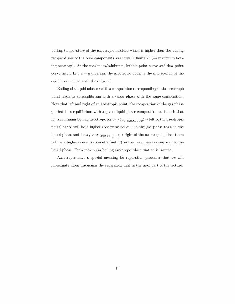
boiling temperature of the azeotropic mixture which is higher than the boiling
temperatures of the pure components as shown in figure 23 (→ maximum boil-
ing azeotrop). At the maximum/minimum, bubble point curve and dew point
curve meet. In a x − y diagram, the azeotropic point is the intersection of the
equilibrium curve with the diagonal.
Boiling of a liquid mixture with a composition corresponding to the azeotropic
point leads to an equilibrium with a vapor phase with the same composition.
Note that left and right of an azeotropic point, the composition of the gas phase
y1 that is in equilibrium with a given liquid phase composition x1 is such that
for a minimum boiling azeotrope for x1 < x1,azeotrope(→ left of the azeotropic
point) there will be a higher concentration of 1 in the gas phase than in the
liquid phase and for x1 > x1,azeotrope (→ right of the azeotropic point) there
will be a higher concentration of 2 (not 1!) in the gas phase as compared to the
liquid phase. For a maximum boiling azeotrope, the situation is inverse.
Azeotropes have a special meaning for separation processes that we will
investigate when discussing the separation unit in the next part of the lecture.
70
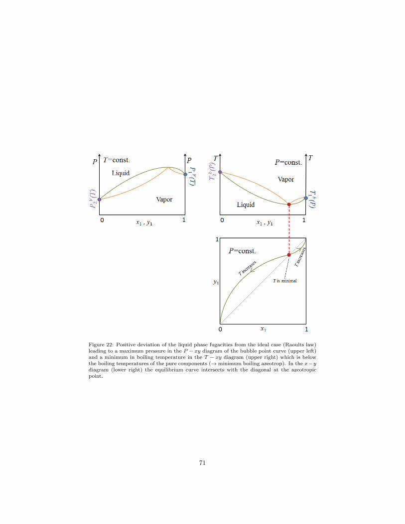
Figure 22: Positive deviation of the liquid phase fugacities from the ideal case (Raoults law)leading to a maximum pressure in the P − xy diagram of the bubble point curve (upper left)and a minimum in boiling temperature in the T − xy diagram (upper right) which is belowthe boiling temperatures of the pure components (→ minimum boiling azeotrop). In the x−ydiagram (lower right) the equilibrium curve intersects with the diagonal at the azeotropicpoint.
71
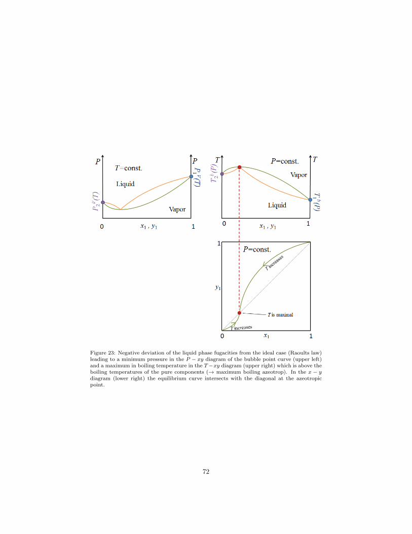
Figure 23: Negative deviation of the liquid phase fugacities from the ideal case (Raoults law)leading to a minimum pressure in the P − xy diagram of the bubble point curve (upper left)and a maximum in boiling temperature in the T−xy diagram (upper right) which is above theboiling temperatures of the pure components (→ maximum boiling azeotrop). In the x − ydiagram (lower right) the equilibrium curve intersects with the diagonal at the azeotropicpoint.
72