Thermal Density Functional Theory in Context∗

Aurora Pribram-Jones,† Stefano Pittalis, E.K.U. Gross, and Kieron BurkeDepartment of Chemistry, University of California, Irvine, CA 92697, USA

CNR–Istituto Nanoscienze, Centro S3, Via Campi 213a, I-41125, Modena, ItalyMax-Planck-Institut fur Mikrostrukturphysik, Weinberg 2, D-06120 Halle, Germany andDepartments of Physics and Chemistry, University of California, Irvine, CA 92697, USA

CONTENTS

I. Abstract 1

II. Introduction 1

III. Density functional theory 2III.1. Introduction 2III.2. Hohenberg-Kohn theorem 3

III.2.1. First part 3III.2.2. Second part 4III.2.3. Consequences 4III.2.4. Extension to degenerate ground

states 4III.3. Kohn-Sham scheme 5

III.3.1. Exchange-correlation energyfunctional 6

III.4. Levy’s formulation 6III.5. Ensemble-DFT and Lieb’s formulation 7

IV. Functional Approximations 8IV.1. Exact Conditions 9

V. Thermal DFT 10

VI. Exact Conditions at Non-Zero Temperature 13

VII. Discussion 14VII.1. Temperature and Coordinate Scaling 14VII.2. Thermal-LDA for Exchange Energies 15VII.3. Exchange-Correlation Hole at Non-Zero

Temperature 15

VIII. Conclusion 16

IX. Acknowledgments 16

References 16

I. ABSTRACT

This chapter introduces thermal density functionaltheory, starting from the ground-state theory and assum-

∗ Appearing in:Computational Challenges in Warm Dense Matter,edited by F. Graziani, et al. (Springer, to be published).† apribram@uci.edu

ing a background in quantum mechanics and statisticalmechanics. We review the foundations of density func-tional theory (DFT) by illustrating some of its key re-formulations. The basics of DFT for thermal ensemblesare explained in this context, as are tools useful for anal-ysis and development of approximations. We close bydiscussing some key ideas relating thermal DFT and theground state. This review emphasizes thermal DFT’sstrengths as a consistent and general framework.

II. INTRODUCTION

The subject matter of high-energy-density physics isvast [1], and the various methods for modeling it are di-verse [2–4]. The field includes enormous temperature,pressure, and density ranges, reaching regimes where thetools of plasma physics are appropriate [5]. But, espe-cially nowadays, interest also stretches down to warmdense matter (WDM), where chemical details can becomenot just relevant, but vital [6]. WDM, in turn, is suffi-ciently close to zero-temperature, ground-state electronicstructure that the methods from that field, especiallyKohn-Sham density functional theory (KS DFT) [7, 8],provide a standard paradigm for calculating material-specific properties with useful accuracy.

It is important to understand, from the outset, that thelogic and methodology of KS-DFT is at times foreign toother techniques of theoretical physics. The proceduresof KS-DFT appear simple, yet the underlying theory issurprisingly subtle. Consequently, progress in develop-ing useful approximations, or even writing down formallycorrect expressions, has been incredibly slow. As the KSmethodology develops in WDM and beyond, it is worthtaking a few moments to wrap one’s head around its logic,as it does lead to one of the most successful paradigmsof modern electronic structure theory [9].

This chapter sketches how the methodology of KS DFTcan be generalized to warm systems, and what new fea-tures are introduced in doing so. It is primarily designedfor those unfamiliar with DFT to get a general under-standing of how it functions and what promises it holdsin the domain of warm dense matter. Section 2 is a gen-eral review of the basic theorems of DFT, using the orig-inal methodology of Hohenberg-Kohn [10] and then themore general Levy-Lieb construction [11, 12]. In Section3, we discuss approximations, which are always neces-sary in practice, and several important exact conditionsthat are used to guide their construction. In Section 4,

Density functional theory

we review the thermal KS equations [13] and some rel-evant statistical mechanics. Section 5 summarizes someof the most important exact conditions for thermal en-sembles [14, 15]. Last, but not least, in Section 6 wereview some recent results that generalize ground-stateexact scaling conditions and note some of the main dif-ferences between the finite-temperature and the ground-state formulation.

III. DENSITY FUNCTIONAL THEORY

A reformulation of the interacting many-electron prob-lem in terms of the electron density rather than themany-electron wavefunction has been attempted sincethe early days of quantum mechanics [16–18]. The ad-vantage is clear: while the wavefunction for interactingelectrons depends in a complex fashion on all the parti-cle coordinates, the particle density is a function of onlythree spatial coordinates.

Initially, it was believed that formulating quantummechanics solely in terms of the particle density givesonly an approximate solution, as in the Thomas-Fermimethod [16–18]. However, in the mid-1960s, Hohenbergand Kohn [10] showed that, for systems of electrons in anexternal potential, all the properties of the many-electronground state are, in principle, exactly determined by theground-state particle density alone.

Another important approach to the many-particleproblem appeared early in the development of quantummechanics: the single-particle approximation. Here, thetwo-particle potential representing the interaction be-tween particles is replaced by some effective, one-particlepotential. A prominent example of this approach is theHartree-Fock method [19, 20], which includes only ex-change contributions in its effective one-particle poten-tial. A year after the Hohenberg-Kohn theorem had beenproven, Kohn and Sham [21] took a giant leap forward.They took the ground state particle density as the basicquantity and showed that both exchange and correlationeffects due to the electron-electron interaction can betreated through an effective single-particle Schrodingerequation. Although Kohn and Sham wrote their paperusing the local density approximation, they also pointedout the exactness of that scheme if the exact exchange-correlation functional were to be used (see Section III.3).The KS scheme is used in almost all DFT calculationsof electronic structure today. Much development in thisfield remains focused on improving approximations to theexchange-correlation energy (see Section IV).

The Hohenberg-Kohn theorem and Kohn-Shamscheme are the basic elements of modern density-functional theory (DFT) [9, 22, 23]. We will reviewthe initial formulation of DFT for non-degenerate groundstates and its later extension to degenerate ground states.Alternative and refined mathematical formulations arethen introduced.

III.1. Introduction

The non-relativistic Hamiltonian1 for N interactingelectrons2 moving in a static potential v(r) reads (inatomic units)

H = T+Vee+V := −1

2

N∑i=1

∇2i+

1

2

N∑i,j=1

i6=j

1

|ri − rj |+

N∑i=1

v(ri).

(1)

Here, T is the total kinetic-energy operator, Vee describesthe repulsion between the electrons, and V is a local(multiplicative) scalar operator. This includes the inter-action of the electrons with the nuclei (considered withinthe Born-Oppenheimer approximation) and any other ex-ternal scalar potentials.

The eigenstates, Ψi(r1, ..., rN ), of the system are ob-tained by solving the eigenvalue problem

HΨi(r1, ..., rN ) = EiΨi(r1, ..., rN ), (2)

with appropriate boundary conditions for the physicalproblem at hand. Eq. (2) is the time-independentSchrodinger equation. We are particularly interested inthe ground state, the eigenstate with lowest energy, andassume the wavefunction can be normalized.

Due to the interactions among the electrons, Vee, anexplicit and closed solution of the many-electron problemin Eq. (2) is, in general, not possible. But because accu-rate prediction of a wide range of physical and chemicalphenomena requires inclusion of electron-electron inter-action, we need a path to accurate approximate solutions.

Once the number of electrons with Coulombic inter-action is given, the Hamiltonian is determined by speci-fying the external potential. For a given v(r), the totalenergy is a functional of the many-body wavefunctionΨ(r1, ..., rN )

Ev[Ψ] = 〈Ψ|T + Vee + V |Ψ〉 . (3)

The energy functional in Eq. (3) may be evaluated forany N -electron wavefunction, and the Rayleigh-Ritz vari-ational principle ensures that the ground state energy,Ev, is given by

Ev = infΨEv[Ψ], (4)

where the infimum is taken over all normalized, antisym-metric wavefunctions. The Euler-Lagrange equation ex-pressing the minimization of the energy is

δ

δΨEv[Ψ]− µ [〈Ψ|Ψ〉 − 1] = 0, (5)

1 See Refs. [24] or [25] for quantum mechanical background thatis useful for this chapter.

2 In this work, we discuss only spin-unpolarized electrons.

2

Hohenberg-Kohn theorem Density functional theory

where the functional derivative is performed over Ψ ∈L2(R3N ) (defined as in Ref. [26]). Relation (5) againleads to the many-body Schrodinger equation and theLagrangian multiplier µ can be identified as the chemicalpotential.

We now have a procedure for finding approximate so-lutions by restricting the form of the wavefunctions. Inthe Hartree-Fock (HF) approximation, for example, theform of the wave-function is restricted to a single Slaterdeterminant. Building on the HF wavefunction, modernquantum chemical methods can produce extremely accu-rate solutions to the Schrodinger equation [27]. Unfor-tunately, wavefunction-based approaches that go beyondHF usually are afflicted by an impractical growth of thenumerical effort with the number of particles. Inspiredby the Thomas-Fermi approach, one might wonder if therole played by the wavefunction could be played by theparticle density, defined as

n(r) := 〈Ψ|N∑i=1

δ(r− ri)|Ψ〉

= N

∫dr2...

∫drN

∣∣∣Ψ(r, r2, ..., rN )∣∣∣2, (6)

from which ∫d3r n(r) = N. (7)

In that case, one would deal with a function of only threespatial coordinates, regardless of the number of electrons.

III.2. Hohenberg-Kohn theorem

Happily, the two-part Hohenberg-Kohn (HK) Theoremassures us that the electronic density alone is enough todetermine all observable quantities of the systems. Theseproofs cleverly connect specific sets of densities, wave-functions, and potentials, exposing a new framework forthe interacting many-body problem.

Let P be the set of external potentials leading to anon-degenerate ground state for N electrons. For a givenpotential, the corresponding ground state, Ψ, is obtainedthrough the solution of the Schrodinger equation:

v −→ Ψ, with v ∈ P. (8)

Wavefunctions obtained this way are called interactingv-representable. We collect these ground state wavefunc-tions in the set W. The corresponding particle densitiescan be computed using definition (6):

Ψ −→ n, with Ψ ∈W. (9)

Ground state particle densities obtained this way are alsocalled interacting v-representable. We denote the set ofthese densities as D.

III.2.1. First part

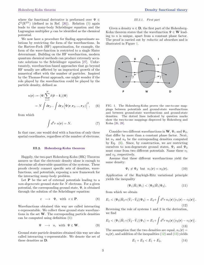
Given a density n ∈ D, the first part of the Hohenberg-Kohn theorem states that the wavefunction Ψ ∈W lead-ing to n is unique, apart from a constant phase factor.The proof is carried out by reductio ad absurdum and isillustrated in Figure 1.

P W D

II I

? ?

FIG. 1. The Hohenberg-Kohn proves the one-to-one map-pings between potentials and ground-state wavefunctionsand between ground-state wavefunctions and ground-statedensities. The dotted lines indicated by question marksshow the two-to-one mappings disproved by Hohenberg andKohn [26, 28].

Consider two different wavefunctions in W, Ψ1 and Ψ2,that differ by more than a constant phase factor. Next,let n1 and n2 be the corresponding densities computedby Eq. (6). Since, by construction, we are restrictingourselves to non-degenerate ground states, Ψ1 and Ψ2

must come from two different potentials. Name these v1

and v2, respectively.Assume that these different wavefunctions yield the

same density:

Ψ1 6= Ψ2 but n1(r) = n2(r). (10)

Application of the Rayleigh-Ritz variational principleyields the inequality

〈Ψ1|H1|Ψ1〉 < 〈Ψ2|H1|Ψ2〉, (11)

from which we obtain

E1 < 〈Ψ2|H2+(V1−V2)|Ψ2〉 = E2+

∫d3r n1(r) [v1(r)− v2(r)] .

(12)Reversing the role of systems 1 and 2 in the derivation,we find

E2 < 〈Ψ1|H1+(V2−V1)|Ψ1〉 = E1+

∫d3r n2(r) [v2(r)− v1(r)] .

(13)The assumption that the two densities are equal, n1(r) =n2(r), and addition of the inequalities (12) and (13) yields

E1 + E2 < E1 + E2, (14)

3

Hohenberg-Kohn theorem Density functional theory

which is a contradiction. We conclude that the forego-ing hypothesis (10) was wrong, so n1 6= n2. Thus eachdensity is the ground-state density of, at most, one wave-function. This mapping between the density and wave-function is written

n −→ Ψ, with n ∈ D and Ψ ∈W. (15)

III.2.2. Second part

Having specified the correspondence between densityand wavefunction, Hohenberg and Kohn then considerthe potential. By explicitly inverting the Schrodingerequation,

N∑i=1

v(ri) = E −

(T + Vee

)Ψ(r1, r2, ..., rN )

Ψ(r1, r2, ..., rN ), (16)

they show the elements Ψ of W also determine the ele-ments v of P, apart from an additive constant.

We summarize this second result by writing

Ψ −→ v, with Ψ ∈W and v ∈ P. (17)

III.2.3. Consequences

Together, the first and second parts of the theoremyield

n −→ v + const, with n ∈ D and v ∈ P, (18)

that the ground state particle density determines the ex-ternal potential up to a trivial additive constant. This isthe first HK theorem.

Moreover, from the first part of the theorem it fol-lows that any ground-state observable is a functional ofthe ground-state particle density. Using the one-to-onedependence of the wavefunction, Ψ[n], on the particledensity,

〈Ψ|O|Ψ〉 = 〈Ψ[n]|O|Ψ[n]〉 = O[n]. (19)

For example, the following functional can be defined:

Ev,HK[n] := 〈Ψ[n]|T + Vee + V |Ψ[n]〉

= FHK[n] +

∫d3r n(r)v(r), (20)

where v is a given external potential and n can be anydensity in D. Note that

FHK[n] := 〈Ψ[n]|T + Vee|Ψ[n]〉 (21)

is independent of v. The second HK theorem is simplythat FHK[n] is independent of v(r). This is therefore auniversal functional of the ground-state particle density.

We use the subscript, HK, to emphasize that this is theoriginal density functional of Hohenberg and Kohn.

Let n0 be the ground-state particle density of the po-tential v0. The Rayleigh-Ritz variational principle (4)immediately tells us

Ev0 = minn∈D

Ev0,HK[n] = Ev0,HK[n0]. (22)

We have finally obtained a variational principle basedon the particle density instead of the computationallyexpensive wavefunction.

III.2.4. Extension to degenerate ground states

The Hohenberg-Kohn theorem can be generalized byallowing P to include local potentials having degener-ate ground states [11, 28, 29], . This means an entiresubspace of wavefunctions can correspond to the lowesteigenvalue of the Schrodinger equation (2). The sets Wand D are enlarged accordingly, to include all the addi-tional ground-state wavefunctions and particle densities.

In contrast to the non-degenerate case, the solutionof the Schrodinger equation (2) now establishes a map-ping from P to W which is one-to-many (see Figure 2).Moreover, different degenerate wavefunctions can havethe same particle density. Equation (6), therefore, es-tablishes a mapping from W to D that is many-to-one.However, any one of the degenerate ground-state densi-ties still determines the potential uniquely.

FIG. 2. The mappings between sets of potentials, wavefunc-tions, and densities can be extended to include potentials withdegenerate ground states. This is seen in the one-to-manymappings between P and W. Note also the many-to-onemappings from W to D caused by this degeneracy [28, 30].

The first part of the HK theorem needs to be mod-ified in light of this alteration of the mapping betweenwavefunctions and densities. To begin, note that two de-generate subspaces, sets of ground states of two differentpotentials, are disjoint. Assuming that a common eigen-state Ψ can be found, subtraction of one Schrodinger

4

Kohn-Sham scheme Density functional theory

equation from the other yields

(V1 − V2)Ψ = (E1 − E2)Ψ. (23)

For this identity to be true, the eigenstate Ψ must vanishin the region where the two potentials differ by more thanan additive constant. This region has measure greaterthan zero. Eigenfunctions of potentials in P, however,vanish only on sets of measure zero [31]. This contradic-tion lets us conclude that v1 and v2 cannot have commoneigenstates. We then show that ground states from twodifferent potentials always have different particle densi-ties using the Rayleigh-Ritz variational principle as inthe non-degenerate case.

However, two or more degenerate ground state wave-functions can have the same particle density. As a conse-quence, neither the wavefunctions nor a generic groundstate property can be determined uniquely from knowl-edge of the ground state particle density alone. Thisdemands reconsideration of the definition of the univer-sal FHK as well. Below, we verify that the definitionof FHK does not rely upon one-to-one correspondenceamong ground state wavefunctions and particle densities.

The second part of the HK theorem in this case pro-ceeds as in the original proof, with each ground state ina degenerate level determining the external potential upto an additive constant. Combining the first and secondparts of the proof again confirms that any element of Ddetermines an element of P, up to an additive constant.In particular, any one of the degenerate densities deter-mines the external potential. Using this fact and that thetotal energy is the same for all wavefunctions in a givendegenerate level, we define FHK:

FHK[n] := E [v[n]]−∫d3r v[n](r)n(r). (24)

This implies that the value of

FHK[n] = 〈Ψ0 → n|T + Vee|Ψ0 → n〉 (25)

is the same for all degenerate ground-state wavefunctionsthat have the same particle density. The variational prin-ciple based on the particle density can then be formulatedas before in Eq. (22).

III.3. Kohn-Sham scheme

The exact expressions defining FHK in the previoussection are only formal ones. In practice, FHK must beapproximated. Finding approximations that yield use-fully accurate results turns out to be an extremely diffi-cult task, so much so that pure, orbital-free approxima-tions for FHK are not pursued in most modern DFT cal-culations. Instead, efficient approximations can be con-structed by introducing the Kohn-Sham scheme, in whicha useful decomposition of FHK in terms of other densityfunctionals is introduced. In fact, the Kohn-Sham de-composition is so effective that effort on orbital-free DFT

utilizes the Kohn-Sham structure, but not its explicitlyorbital-dependent expressions.

Consider the Hamiltonian of N non-interacting elec-trons

Hs = T + V := −1

2

N∑i=1

∇2i +

N∑i=1

v(ri). (26)

Mimicking our procedure with the interacting system, wegroup external local potentials in the set P. The corre-sponding non-interacting ground state wavefunctions Ψs

are then grouped in the set Ws, and their particle den-sities ns are grouped in Ds. We can then apply the HKtheorem and define the non-interacting analog of FHK,which is simply the kinetic energy:

Ts[ns] := E [v[ns]]−∫d3r v[ns](r)ns(r). (27)

Restricting ourselves to non-degenerate ground states,the expression in Eq. (27) can be rewritten to stress theone-to-one correspondence among densities and wave-functions:

Ts[ns] = 〈Ψs[ns]|T |Ψs[ns]〉 . (28)

We now introduce a fundamental assumption: for eachelement n of D, a potential vs in Ps exists, with corre-sponding ground-state particle density ns = n. We callvs the Kohn-Sham potential. In other words, interact-ing v-representable densities are also assumed to be non-interacting v-representable. This maps the interactingproblem onto a non-interacting one.

Assuming the existence of vs, the HK theorem appliedto the class of non-interacting systems ensures that vs isunique up to an additive constant. As a result, we findthe particle density of the interacting system by solvingthe non-interacting eigenvalue problem, which is calledthe Kohn-Sham equation:

HsΦ = EΦ. (29)

For non-degenerate ground states, the Kohn-Shamground-state wavefunction is a single Slater determinant.In general, when considering degenerate ground states,the Kohn-Sham wavefunction can be expressed as a lin-ear combination of several Slater determinants [12, 32].There also exist interacting ground states with particledensities that can only be represented by an ensemble ofnon-interacting particle densities [33–37]. We will comeback to this point in Section III.5.

Here we continue by considering the simplest cases ofnon-degenerate ground states. Eq. (29) can be rewrittenin terms of the single-particle orbitals as follows:[

−1

2∇2 + vs(r)

]ϕi(r) = εiϕi(r) . (30)

The single-particle orbitals ϕi(r) are called Kohn-Shamorbitals and Kohn-Sham wavefunctions are Slater deter-minants of these orbitals. Via the Kohn-Sham equa-tions, the orbitals are implicit functionals of n(r). We

5

Kohn-Sham scheme Density functional theory

emphasize that – although in DFT the particle densityis the only basic variable – the Kohn-Sham orbitals areproper fermionic single-particle states. The ground-stateKohn-Sham wavefunction is obtained by occupying theN eigenstates with lowest eigenvalues. The correspond-ing density is

n(r) =

N∑i=1

ni|ϕi(r)|2, (31)

with ni the ith occupation number.In the next section, we consider the consequences of

introducing the Kohn-Sham system in DFT.

III.3.1. Exchange-correlation energy functional

A large fraction of FHK[n] can be expressed in termsof kinetic and electrostatic energy. This decompositionis given by

FHK[n] = Ts[n] + U [n] + Exc[n] . (32)

The first term is the kinetic energy of the Kohn-Shamsystem,

Ts[n] = −1

2

N∑i=1

∫d3r ϕ∗i (r)∇2ϕi(r) . (33)

The second is the Hartree energy (a.k.a. electrostaticself-energy, a.k.a. Coulomb energy),

U [n] =1

2

∫ ∫d3rd3r′

n(r)n(r′)

|r− r′|. (34)

The remainder is defined as the exchange-correlation en-ergy,

Exc[n] := FHK[n]− Ts[n]− U [n] . (35)

For systems having more than one particle, Exc accountsfor exchange and correlation energy contributions. Com-paring Eqs. (32) and (20), the total energy density func-tional is

Ev,HK[n] = Ts[n]+U [n]+Exc[n]+

∫d3r n(r)v(r). (36)

Consider now the Euler equations for the interactingand non-interacting system. Assuming the differentiabil-ity of the functionals (see Section III.5), these necessaryconditions for having energy minima are

δFHK

δn(r)+ v(r) = 0 (37)

and

δTsδn(r)

+ vs(r) = 0, (38)

respectively. With definition (32), from Eqs. (37) and(38), we obtain

vs(r) = vH [n](r) + vxc[n](r) + v(r). (39)

Here, v(r) is the external potential acting upon the in-teracting electrons, vH [n](r) is the Hartree potential,

vH [n](r) =

∫d3r′

n(r′)

|r− r′|=

δU

δn(r), (40)

and vxc[n](r) is the exchange-correlation potential,

vxc[n](r) =δExc[n]

δn(r). (41)

Through the decomposition in Eq. (32), a significantpart of FHK is in the explicit form of Ts[n] + U [n] with-out approximation. Though often small, the Exc densityfunctional still represents an important part of the to-tal energy. Its exact functional form is unknown, and ittherefore must be approximated in practice. However,good and surprisingly efficient approximations exist forExc.

We next consider reformulations of DFT, which allowanalysis and solution of some important technical ques-tions at the heart of DFT. They also have a long historyof influencing the analysis of properties of the exact func-tionals.

III.4. Levy’s formulation

An important consequence of the HK theorem is thatthe Rayleigh-Ritz variational principle based on thewavefunction can be replaced by a variational principlebased on the particle density. The latter is valid for alldensities in the set D, the set of v-representable densities.Unfortunately, v-representability is a condition which isnot easily verified for a given function n(r). Hence itis highly desirable to formulate the variational principleover a set of densities characterized by simpler conditions.This was provided by Levy [11] and later reformulatedand extended by Lieb [12]. In this and the sections thatfollow, Lebesgue and Sobolev spaces are defined in theusual way [26, 38].

First, the set W is enlarged to WN, which includes allpossible antisymmetric and normalized N -particle wave-functions Ψ. The set WN now also contains N -particlewavefunctions which are not necessarily ground-statewavefunctions to some external potential v, though itremains in the same Sobolev space [26] as W: H1(R3N ).Correspondingly, the set D is replaced by the set DN.DN contains the densities generated from the N -particleantisymmetric wavefunctions in WN using Eq. (6):

DN =

n | n(r) ≥ 0,

∫d3r n(r) = N,n1/2(r) ∈ H1(R3)

.

(42)

6

Levy’s formulation Density functional theory

The densities of DN are therefore called N -representable.Harriman’s explicit construction [39] shows that any in-tegrable and positive function n(r) is N -representable.

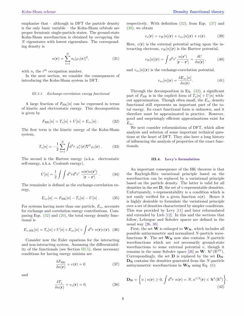
FIG. 3. This diagram shows the two-step minimization ofLevy’s constrained search. The first infimum search is overall wavefunctions corresponding to a certain density ni. Thesecond search runs over all of the densities [30, 40].

Levy reformulated the variational principle in aconstrained-search fashion (see Figure 3):

Ev = infn∈DN

inf

Ψ→n|Ψ∈WN

〈Ψ|T + Vee|Ψ〉+

∫d3r n(r)v(r)

.

(43)In this formulation, the search inside the braces is con-strained to those wavefunctions which yield a given den-sity n – therefore the name “constrained search”. Theminimum is then found by the outer search over all densi-ties. The potential v(r) acts like a Lagrangian multiplierto satisfy the constraint on the density at each point inspace. In this formulation, FHK is replaced by

FLL[n] := infΨ→n〈Ψ|T+Vee|Ψ〉, with Ψ ∈WN and n ∈ DN .

(44)The functional EHK can then be replaced by

Ev,LL[n] := FLL[n] +

∫d3r n(r)v(r), with n ∈ DN.

(45)If, for a given v0, the corresponding ground-state particledensity, n0, is inserted, then

Ev0,LL[n0] = Ev0,HK[n0] = Ev0 , (46)

from which

FLL[n] = FHK[n], for all n ∈ D . (47)

Furthermore, if any other particle density is inserted, weobtain

Ev0,LL[n] ≥ Ev0 , for n 6= n0 and n ∈ DN. (48)

In this approach, the degenerate case does not requireparticular care. In fact, the correspondences between

potentials, wavefunctions and densities are not explic-itly employed as they were in the previous Hohenberg-Kohn formulation. However, the N -representability is ofsecondary importance in the context of the Kohn-Shamscheme. There, it is still necessary to assume that thedensities of the interacting electrons are non-interactingv-representable as well. We discuss this point in moredetail in the next section.

Though it can be shown that the FLL[n] infimumis a minimum [12], the functional’s lack of convexitycauses a serious problem in proving the differentiabil-ity of FLL [12]. Differentiability is needed to define anEuler equation for finding n(r) self-consistently. This issomewhat alleviated by the Lieb formulation of DFT (seebelow).

III.5. Ensemble-DFT and Lieb’s formulation

In the remainder of this section, we are summariz-ing more extensive and pedagogical reviews that can befound in Refs. [26], [28], and [41]. Differentiability offunctionals is, essentially, related to the convexity of thefunctionals. Levy and Lieb showed that the set D is notconvex [12]. In fact, there exist combinations of the form

n(r) =

M∑k=1

λknk(r), λk = 1 (0 ≤ λk ≤ 1), (49)

where nk is the density corresponding to degenerateground state Ψk, that are not in D [12, 42].

A convex set can be obtained by looking at ensembles.The density of an ensemble can be defined through the(statistical, or von Neuman) density operator

D =

M∑k=1

λk|Ψk〉〈Ψk|, with

M∑k=1

λk = 1 (0 ≤ λk ≤ 1) .

(50)

The expectation value of an operator O on an ensembleis defined as

O := TrDO

, (51)

where the symbol “Tr” stands for the trace taken over anarbitrary, complete set of orthonormal N -particle states

TrDO :=∑k

〈Φk|(DO)|Φk〉. (52)

The trace is invariant under unitary transformations ofthe complete set for the ground-state manifold of theHamiltonian H [see Eq.(50)]. Since

TrDO

=

M∑k=1

λk〈Ψk|O|Ψk〉, (53)

the energy obtained from a density matrix of the form(50) is the total ground-state energy of the system.

7

Ensemble-DFT and Lieb’s formulation Functional Approximations

Densities of the form (49) are called ensemble v-representable densities, or E-V-densities. We denote thisset of densities as DEV. Densities that can be obtainedfrom a single wavefunction are said to be pure-state (PS)v-representable, or PS-V-densities. The functional FHK

can then be extended as [43]

FEHK[n] := TrD(T + Vee

), with n ∈ DEV (54)

where D has the form (50) and is any density matrixgiving the density n. However, the set DEV, just likeD, is difficult to characterize. Moreover, as for FHK andFLL, a proof of the differentiability of FEHK (and for thenon-interacting versions of the same functional) is notavailable.

In the Lieb formulation, however, differentiability canbe addressed to some extent [12, 44, 45] . In the workof Lieb, P is restricted to P = L3/2(R3) + L∞(R3) andwavefunctions are required to be in

WN = Ψ | ||Ψ|| = 1, T [Ψ] ≤ ∞ . (55)

The universal functional is defined as

FL[n] := infD→n∈DN

TrD(T + Vee

), (56)

and it can be shown that the infimum is a minimum [12].

Note that in definition (56), D is a generic density matrixof the form

D =∑k

λk|Ψk〉〈Ψk|, with∑k

λk = 1 (0 ≤ λk ≤ 1) ,

(57)where Ψk ∈ WN. The sum is not restricted to a finitenumber of degenerate ground states as in Eq. (50). Thisminimization over a larger, less restricted set leads to thestatements

FL[n] ≤ FLL[n], for n ∈ DN, (58)

and

FL[n] = FLL[n] = FHK[n], for n ∈ D . (59)

FL[n] is defined on a convex set, and it is a convex func-tional. This implies that FL[n] is differentiable at anyensemble v-representable densities and nowhere else [12].Minimizing the functional

EL[n] := FL[n] +

∫d3r n(r)v(r) (60)

with respect to the elements of DEV by the Euler-Lagrange equation

δFL

δn(r)+ v(r) = 0 (61)

is therefore well-defined on the set DEV and generates avalid energy minimum.

We finally address, although only briefly, some impor-tant points about the Kohn-Sham scheme and its rigor-ous justification. The results for FL carry over to TL[n].That is, the functional

TL[n] = infD→n

TrDT, with n ∈ DN (62)

is differentiable at any non-interacting ensemble v-representable densities and nowhere else. We can gatherall these densities in the set Ds

EV. Then, the Euler-Lagrange equation

δTL

δn(r)+ vs(r) = 0 (63)

is well defined on the set DsEV only. One can then rede-

fine the exchange-correlation functional as

Exc,L[n] = FL[n]− TL[n]− U [n], (64)

and observe that the differentiability of FL[n] and TL[n]implies the differentiability of Exc[n] only on DEV∩Ds

EV.The question as to the size of the latter set remains. Fordensities defined on a discrete lattice (finite or infinite)it is known [46] that DEV = Ds

EV. Moreover, in thecontinuum limit, DE and Ds

E can be shown to be densewith respect to one another [12, 44, 45]. This impliesthat any element of DEV can be approximated, with anarbitrary accuracy, by an element of Ds

EV. But, whetheror not the two sets coincide remains an open question.

IV. FUNCTIONAL APPROXIMATIONS

Numerous approximations to Exc exist, each with itsown successes and failures [9]. The simplest is the lo-cal density approximation (LDA), which had early suc-cess with solids[21]. LDA assumes that the exchange-correlation energy density can be approximated locallywith that of the uniform gas. DFT’s popularity in thechemistry community skyrocketed upon development ofthe generalized gradient approximation (GGA) [47]. In-clusion of density gradient dependence generated suffi-ciently accurate results to be useful in many chemicaland materials applications.

Today, many scientists use hybrid functionals, whichsubstitute a fraction of single-determinant exchange forpart of the GGA exchange [48–50]. More recent de-velopments in functional approximations include meta-GGAs [51], which include dependence on the kinetic en-ergy density, and hyper-GGAs [51], which include exactexchange as input to the functional. Inclusion of occupiedand then unoccupied orbitals as inputs to functionals in-creases their complexity and computational cost; the ideathat this increase is coupled with an increase in accuracywas compared to Jacob’s Ladder [51]. The best approxi-mations are based on the exchange-correlation hole, suchas the real space cutoff of the LDA hole that ultimatelyled to the GGA called PBE [52, 53]. An introduction to

8

Exact Conditions Functional Approximations

this and some other exact properties of the functionalsfollows in the remainder of this section.

Another area of functional development of particularimportance to the warm dense matter community is fo-cused on orbital-free functionals [28, 54–57]. These ap-proximations bypass solution of the Kohn-Sham equa-tions by directly approximating the non-interacting ki-netic energy. In this way, they recall the original, pureDFT of Thomas-Fermi theory [16–18]. While many ap-proaches have been tried over the decades, including fit-ting techniques from computer science [58], no general-purpose solution of sufficient accuracy has been foundyet.

IV.1. Exact Conditions

Though we do not know the exact functional form forthe universal functional, we do know some facts aboutits behavior and the relationships between its compo-nents. Collections of these facts are called exact condi-tions. Some can be found by inspection of the formaldefinitions of the functionals and their variational prop-erties. The correlation energy and its constituents aredifferences between functionals evaluated on the true andKohn-Sham systems. As an example, consider the kineticcorrelation:

Tc[n] = T [n]− Ts[n]. (65)

Since the Kohn-Sham kinetic energy is the lowest kineticenergy of any wavefunction with density n(r), we know Tcmust be non-negative. Other inequalities follow similarly,as well as one from noting that the exchange functionalis (by construction) never positive [22]:

Ex ≤ 0, Ec ≤ 0, Uc ≤ 0, Tc ≥ 0. (66)

Some further useful exact conditions are found by uni-form coordinate scaling [59]. In the ground state, thisprocedure requires scaling all the coordinates of the wave-function3 by a positive constant γ, while preserving nor-malization to N particles:

Ψγ(r1, r2, ..., rN) = γ3N/2Ψ(γr1, γr2, ..., γrN), (67)

which has a scaled density defined as

nγ(r) = γ3n(γr). (68)

Scaling by a factor larger than one can be thought of assqueezing the density, while scaling by γ < 1 spreads the

3 Here and in the remainder of the chapter, we restrict ourselvesto square-integrable wavefunctions over the domain R3N .

density out. For more details on the many conditionsthat can be extracted using this technique and how theycan be used in functional approximations, see Ref. [22].

Of greatest interest in our context are conditions in-volving exchange-correlation and other components ofthe universal functional. Through application of the fore-going definition of uniform scaling, we can write downsome simple uniform scaling equalities. Scaling the den-sity yields

Ts[nγ ] = γ2Ts[n] (69)

for the non-interacting kinetic energy and

Ex[nγ ] = γ Ex[n] (70)

for the exchange energy. Such simple conditions arise be-cause these functionals are defined on the non-interactingKohn-Sham Slater determinant. On the other hand, al-though the density from a scaled interacting wavefunc-tion is the scaled density, the scaled wavefunction is notthe ground-state wavefunction of the scaled density. Thismeans correlation scales less simply and only inequalitiescan be derived for it.

Another type of scaling that is simply related to coordi-nate scaling is interaction scaling, the adiabatic change ofthe interaction strength [60]. In the latter, the electron-electron interaction in the Hamiltonian, Vee, is multipliedby a factor, λ between 0 and 1, while holding n fixed.When λ = 0, interaction vanishes. At λ = 1, we return tothe Hamiltonian for the fully interacting system. Due tothe simple, linear scaling of Vee with coordinate scaling,we can relate it to scaling of interaction strength. Com-bining this idea with some of the simple equalities aboveleads to one of the most powerful relations in ground-state functional development, the adiabatic connectionformula [61, 62]:

Exc[n] =

∫ 1

0

dλUxc[n](λ), (71)

where

Uxc[n](λ) = Vee[Ψλ[n]]− U [n] (72)

and Ψλ[n] is the ground-state wavefunction of density nfor a given λ and

Ψλ[n](r1, r2, ..., rN) = λ3N/2Ψ[n1/λ](λr1, λr2, ..., λrN).(73)

Interaction scaling also leads to some of the most im-portant exact conditions for construction of functionalapproximations, the best of which are based on theexchange-correlation hole. The exchange-correlation holerepresents an important effect of an electron sitting ata given position. All other electrons will be kept awayfrom this position by exchange and correlation effects,due to the antisymmetry requirement and the Coulombrepulsion, respectively. This representation allows us to

9

Exact Conditions Thermal DFT

calculate Vee, the electron-electron repulsion, in terms ofan electron distribution function.4

To define the hole distribution function, we need firstto introduce the pair density function. The pair density,P (r, r′) describes the distribution of the electron pairs.This is proportional to the the probability of finding anelectron in a volume d3r around position r and a secondelectron in the volume d3r′ around r′. In terms of theelectronic wavefunction, it is written as follows

P (r, r′) = N(N−1)

∫d3r3 . . .

∫d3rN |Ψ(r, r′, . . . , rN )|2.

(74)We then can define the conditional probability density offinding an electron in d3r′ after having already found oneat r, which we will denote n2(r, r′). Thus

n2(r, r′) = P (r, r′)/n(r). (75)

If the positions of the electrons were truly independent ofone another (no electron-electron interaction and no an-tisymmetry requirement for the wavefunction) this wouldbe just n(r′), independent of r. But this cannot be, as∫

d3r′ n2(r, r′) = N − 1. (76)

The conditional density integrates to one fewer electron,since one electron is at the reference point. We thereforedefine a “hole” density:

n2(r, r′) = n(r′) + nhole(r, r′). (77)

which is typically negative and integrates to -1 [60]:∫d3r′ nhole(r, r′) = −1. (78)

The exchange-correlation hole in DFT is given by thecoupling-constant average:

nxc(r, r′) =

∫ 1

0

dλ nλhole(r, r′), (79)

where nλhole is the hole in Ψλ. So, via the adiabaticconnection formula (Eq. 71), the exchange-correlationenergy can be written as a double integral over theexchange-correlation hole:

Exc =1

2

∫d3r n(r)

∫d3r′

nxc(r, r′)

|r− r′|. (80)

By definition, the exchange hole is given by nx = nλ=0hole

and the correlation hole, nc, is everything not in nx. Theexchange hole may be readily obtained from the (ground-state) pair-correlation function of the Kohn-Sham sys-tem. Moreover nx(r, r) = 0, nx(r, r′) ≤ 0, and for one

4 For a more extended discussion of these topics, see Ref. [60].

particle systems nx(r, r′) = −n(r′). If the Kohn-Shamstate is a single Slater determinant, then the exchangeenergy assumes the form of the Fock integral evaluatedwith occupied Kohn-Sham orbitals. It is straightforwardto verify that the exchange-hole satisfies the sum rule∫

d3r′ nx(r, r′) = −1 ; (81)

and thus ∫d3r′ nc(r, r

′) = 0 . (82)

The correlation hole is a more complicated quantity, andits contributions oscillate from negative to positive insign. Both the exchange and the correlation hole decayto zero at large distances from the reference position r.

These and other conditions on the exact hole are usedto constrain exchange-correlation functional approxima-tions. The seemingly unreasonable reliability of the sim-ple LDA has been explained as the result of the “cor-rectness” of the LDA exchange-correlation hole [63, 64].Since the LDA is constructed from the uniform gas, whichhas many realistic properties, its hole satisfies manymathematical conditions on this quantity [65]. Many ofthe most popular improvements on LDA, including thePBE generalized gradient approximation, are based onmodels of the exchange-correlation hole, not just fits ofexact conditions or empirical data [52]. In fact, the mostsuccessful approximations usually are based on modelsfor the exchange-correlation hole, which can be explicitlytested [66]. Unfortunately, insights about the ground-state exchange-correlation hole do not simply generalizeas temperatures increase, as will be discussed later.

V. THERMAL DFT

Thermal DFT deals with statistical ensembles of quan-tum states describing the thermodynamical equilibriumof many-electron systems. The grand canonical ensem-ble is particularly convenient to deal with the symmetryof identical particles. In the limit of vanishing temper-ature, thermal DFT reduces to an equiensemble groundstate DFT description [67], which, in turn, reduces to thestandard pure-state approach for non-degenerate cases.

While in the ground-state problem the focus is on theground state energy, in the statistical mechanical frame-work the focus is on the grand canonical potential. Here,the grand canonical Hamiltonian plays an analogous roleas the one played by the Hamiltonian for the ground-stateproblem. The former is written

Ω = H − τ S − µN, (83)

where H, S, and N are the Hamiltonian, entropy, andparticle-number operators. The crucial quantity bywhich the Hamiltonian differs from its grand-canonical

10

Thermal DFT

version is the entropy operator:5

S = − kB ln Γ , (84)

where

Γ =∑N,i

wN,i|ΨN,i〉〈ΨN,i| . (85)

|ΨN,i〉 are orthonormal N -particle states (that are notnecessarily eigenstates in general) and wN,i are normal-

ized statistical weights satisfying∑N,i wN,i = 1. Γ al-

lows us to describe the thermal ensembles of interest.Observables are obtained from the statistical average

of Hermitian operators

O[Γ] = Tr ΓO =∑N

∑i

wN,i〈ΨN,i|O|ΨN,i〉 . (86)

These expressions are similar to Eq. (53), but here thetrace is not restricted to the ground-state manifold.

In particular, consider the average of the Ω, Ω[Γ], andsearch for its minimum at a given temperature, τ , andchemical potential, µ. The quantum version of the GibbsPrinciple ensures that the minimum exists and is unique(we shall not discuss the possible complications intro-duced by the occurrence of phase transitions). The min-imizing statistical operator is the grand-canonical statis-tical operator, with statistical weights given by

w0N,i =

exp[−β(E0N,i − µN)]∑

N,i exp[−β(E0N,i − µN)]

. (87)

E0N,i are the eigenvalues of N -particle eigenstates. It can

be verified that Ω[Γ] may be written in the usual form

Ω = E − τS − µN = −kBτ lnZG, (88)

where ZG is the grand canonical partition function; whichis defined by

ZG =∑N

∑j

e−β(E0N,i−µN) . (89)

The statistical description we have outlined so far is thestandard one. Now, we wish to switch to a density-baseddescription and thereby enjoy the same benefits as in theground-state problem. To this end, the minimization ofΩ can be written as follows:

Ωτv−µ = minn

F τ [n] +

∫d3r n(r)(v(r)− µ)

(90)

with n(r) an ensemble N -representable density and

F τ [n] := minΓ→n

F τ [Γ] = minΓ→n

T [Γ] + Vee[Γ]− τS[Γ]

.

(91)

5 Note that, we eventually choose to work in a system of units suchthat the Boltzmann constant is kB = 1, that is, temperature ismeasured in energy units.

This is the constrained-search analog of the Levy func-tional [11, 40], Eq. (44). It replaces the functional orig-inally defined by Mermin [13] in the same way thatEq. (44) replaces Eq. (21) in the ground-state theory.6

Eq. (91) defines the thermal universal functional. Uni-versality of this quantity means that it does not dependexplicitly on the external potential nor on µ. This is veryappealing, as it hints at the possibility of widely applica-ble approximations.

We identify Γτ [n] as the minimizing statistical oper-ator in Eq. (91). We can then define other interactingdensity functionals at a given temperature by taking thetrace over the given minimizing statistical operator. Forexample, we have:

T τ [n] := T [Γτ [n]] (92)

V τee[n] := Vee[Γτ [n]] (93)

Sτ [n] := S[Γτ [n]]. (94)

In order to introduce the thermal Kohn-Sham sys-tem, we proceed analogously as in the zero-temperaturecase. We assume that there exists an ensemble ofnon-interacting systems with same average particle den-sity and temperature of the interacting ensemble. Ulti-mately, this determines the one-body Kohn-Sham poten-tial, which includes the corresponding chemical poten-tial. Thus, the noninteracting (or Kohn-Sham) universalfunctional is defined as

F τs [n] := minΓ→n

Kτ [Γ] = Kτ [Γτs [n]] = Kτs [n], (95)

where Γτs [n] is a statistical operator that describes the

Kohn-Sham ensemble and Kτ [Γ] := T [Γ] − τS[Γ] is acombination we have chosen to call the kentropy.

We can also write the corresponding Kohn-Sham equa-tions at non-zero temperature, which are analogous toEqs. (30) and (39) [21]:[

−1

2∇2 + vs(r)

]ϕi(r) = ετi ϕi(r) (96)

vs(r) = vH [n](r) + vxc[n](r) + v(r). (97)

The accompanying density formula is

n(r) =∑i

fi|ϕi(r)|2, (98)

where

fi =(

1 + e(ετi−µ)/τ)−1

. (99)

6 The interested reader may find the extension of the Hohenberg-Kohn theorem to the thermal framework in Mermin’s paper.

11

Thermal DFT

Eqs. (96) and (97) look strikingly similar to the caseof non-interacting Fermions. However, the Kohn-Shamweights, fi, are not simply the familiar Fermi functions,due to the temperature dependence of the Kohn-Shameigenvalues.

Through the series of equalities in Eq. (95), we seethat the non-interacting universal density functional isobtained by evaluating the kentropy on a non-interacting,minimizing statistical operator which, at temperature τ ,yields the average particle density n. The seemingly sim-ple notation of Eq. (95) reduces the kentropy first in-troduced as a functional of the statistical operator to afinite-temperature functional of the density. From thesame expression, we see that the kentropy plays a rolein this framework analogous to that of the kinetic en-ergy within ground-state DFT. Finally, we spell-out thecomponents of F τs [n]:

F τs [n] = T τs [n]− τSτs [n] , (100)

where T τs [n] := T [Γτs [n]] and Sτs [n] := S[Γτs [n]].Now we identify other fundamental thermal DFT

quantities. First, consider the decomposition of the in-teracting grand-canonical potential as a functional of thedensity given by

Ωτv−µ[n] = F τs [n]+U [n]+Fτxc[n]+

∫d3r n(r) (v(r)− µ) .

(101)Here, U [n] is the Hartree energy having the form inEq. (34). The adopted notation stresses that temper-ature dependence of U [n] enters only through the in-put equilibrium density. The exchange-correlation free-energy density functional is given by

Fτxc[n] = F τ [n]− F τs [n]− U [n] . (102)

It is also useful to introduce a further decomposition:

Fτxc[n] := Fτx [n] + Fτc [n] . (103)

This lets us analyze the two terms on the right hand sidealong with their components.

The exchange contribution is

Fτx [n] = Vee[Γτs [n]]− U [n] . (104)

Note that the average on the right hand side is takenwith respect to the Kohn-Sham ensemble and that ki-netic and entropic contributions do not contribute to ex-change effects explicitly. Interaction enters in Eq. (104)in a fashion that is reminiscent of (but not the same as)finite-temperature Hartree-Fock theory. In fact, Fτx [n]may be expressed in terms of the square modulus of thefinite-temperature Kohn-Sham one-body density matrix.Thus Fτx [n] has an explicit, known expression, just asdoes Fτs [n]. For the sake of practical calculations, how-ever, approximations are still needed.

The fundamental theorems of density functional the-ory were proven for any ensemble with monotonically

decreasing weights [68] and were applied to extract ex-citations [69–71]. But simple approximations to the ex-change for such ensembles are corrupted by ghost inter-actions [72] contained in the ensemble Hartree term. TheHartree energy defined in Eq. (34) is defined as the elec-trostatic self-energy of the density, both for ground-stateDFT and at non-zero temperatures. But the physicalensemble of Hartree energies is in fact the Hartree en-ergy of each ensemble member’s density, added togetherwith the weights of the ensembles. Because the Hartreeenergy is quadratic in the density, it therefore containsghost interactions [72], i.e., cross terms, that are unphys-ical. These must be canceled by the exchange energy,which must therefore contain a contribution:

∆EGIX =∑i

wiU [ni]− U

[∑i

wini

]. (105)

Such terms appear only when the temperature is non-zeroand so are missed by any ground-state approximation toEx.

Consider, now, thermal DFT correlations. We mayexpect correctly that these will be obtained as differ-ences between interacting averages and the noninteract-ing ones. The kinetic correlation energy density func-tional is

T τc [n] := T τ [n]− T τs [n], (106)

and similar forms apply to Sτc [n] and Kτc [n]. Another

important quantity is the correlation potential densityfunctional. At finite-temperature, this is defined by

Uτc [n] := Vee[Γτ [n]]− Vee[Γτs [n]] . (107)

Finally, we can write the correlation free energy as fol-lows

Fτc [n] = Kτc [n] + Uτc [n] = Eτc [n]− τSτc [n] (108)

where

Kτc [n] = T τc [n]− τSτc [n] (109)

is the correlation kentropy density functional and

Eτc [n] := T τc [n] + Uτc [n] (110)

generalizes the expression of the correlation energy to fi-nite temperature. Above, we have noticed that entropiccontributions do not enter explicitly in the definition ofFτx [n]. From Eq. (108), on the other hand, we see thatthe correlation entropy is essential for determining Fτc [n].Further, it may be grouped together the kinetic contri-butions (as in the first identity) or separately (as in thesecond identity), depending on the context of the currentanalysis.

In the next section, we consider finite-temperatureanalogs of the exact conditions described earlier for theground state functionals. This allow us to gain additionalinsights about the quantities identified so far.

12

Exact Conditions at Non-Zero Temperature

VI. EXACT CONDITIONS AT NON-ZEROTEMPERATURE

In the following, we review several properties of the ba-sic energy components of thermal Kohn-Sham DFT [14,15].

We start with some of the most elementary properties,their signs [14]:

Fτx [n] ≤ 0, Fτc [n] ≤ 0, Uτc [n] ≤ 0, Kτc [n] ≥ 0. (111)

The sign of Fτx [n] is evident from the definition given interms of the Kohn-Sham one-body reduced density ma-trix [26]. The others may be understood in terms of theirvariational properties. For example, let us consider thecase for Kτ

c [n]. We know that the Kohn-Sham statisticaloperator minimizes the kentropy

Kτs [n] = Kτ [Γτs [n]] . (112)

Thus, we also know thatKτs [n] must be less thanKτ [n] =

Kτ [Γτ [n]], where Γτ [n] is the equilibrium statistical op-erator. This readily implies that

Kτc [n] = Kτ [Γτ [n]]−Kτ [Γτs [n]] ≥ 0. (113)

An approximation for Kτc [n] that does not respect this

inequality will not simply have the “wrong” sign. Muchworse is that results from such an approximation willsuffer from improper variational character.

A set of remarkable and useful properties are thescaling relationships. What follows mirrors the zero-temperature case, but an important and intriguing dif-ference is the relationship between coordinate and tem-perature scaling.

We first introduce the concept of uniform scaling ofstatistical ensembles in terms of a particular scaling ofthe corresponding statistical operators. 7 Wavefunctionsof each state in the ensemble can be scaled as in Eq. (67).At the same time, we require that the statistical mixingis not affected, so the statistical weights are held fixedunder scaling (we shall return to this point in SectionVII.1). In summary, the scaled statistical operator is

Γγ :=∑N

∑i

wN,i|Ψγ,N,i〉〈Ψγ,N,i|, (114)

where (the representation free) Hilbert space element|Ψγ〉 is such that Ψγ(r1, ..., rN ) = 〈r1, ..., rN |Ψγ〉. Forsake of simplicity, we restrict ourselves to states of thetype typically considered in the ground-state formalism.

7 Uniform coordinate scaling may be considered as (very) care-ful dimensional analysis applied to density functionals. Duftyand Trickey analyze non-interacting functionals in this way inRef. [15].

Eq. (114) leads directly to scaling relationships for anyobservable. For instance, we find

N [Γγ ] = N [Γ], (115)

T [Γγ ] = γ2T [Γ], and (116)

S[Γγ ] = S[Γ] . (117)

Combining these, we find

Γτs [nγ ] = Γτ/γ2

γ,s [n] and F τs [nγ ] = γ2F τ/γ2

s [n]. (118)

Eq. (118) states that the value of the non-interacting uni-versal functional evaluated at a scaled density is relatedto the value of the same functional evaluated on the un-scaled density at a scaled temperature. Eq. (118) consti-tutes a powerful statement, which becomes more appar-ent by rewriting it as follows [14]:

F τ′

s [n] =τ ′

τF τs [n√

τ/τ ′ ]. (119)

This means that, if we know F τs [n] at some non-zero tem-perature τ , we can find its value at any other temperatureby scaling its argument.

Scaling arguments allow us to extract other propertiesof the functionals, such as some of their limiting behav-iors. For instance, we can show that in the “high-density”limit, the kinetic term dominates [14]:

T∞s [n] = limγ→+∞

Fs[nγ ]/τ2 (120)

while in the “low-density” limit, the entropic term dom-inates:

S∞s [n] = limγ→0

Fs[nγ ]τ. (121)

Also, we may consider the interacting universal func-tional for a system with coupling strength equal to λ

F τ,λ[n] = minΓ→n

T [Γ] + λVee[Γ]− τS[Γ]

, (122)

and note that in general,

Γτ,λ[n] 6= Γτ [n]. (123)

We can relate these two statistical operators [14]. In fact,one can prove

Γτ,λ[n] = Γτ/λ2

λ [n1/λ] and F τ,λ[n] = λ2F τ/λ2

[n1/λ].(124)

In the expressions above, a single superscript implies fullinteraction [14]. Eq. (124) demands scaling of the coor-dinates, the temperature, and the strength of the inter-action at once. This procedure connects one equilibriumstate to another equilibrium state, that of a “scaled” sys-tem. Eq. (124) may be used to state other relations simi-lar to those discussed above for the non-interacting case.

13

Discussion

Scaling relations combined with the Hellmann-Feynman theorem allow us to generate the thermal ana-log of one of the most important statements of ground-state DFT, the adiabatic connection formula [14]:

Fτxc[n] =

∫ 1

0

dλ Uτxc[n](λ), (125)

where

Uτxc[n](λ) = Vee[Γτ,λ[n]]− U [n] (126)

and a superscript λ implies an electron-electron interac-tion strength equal to λ. The interaction strength runsbetween zero, corresponding to the noninteracting Kohn-Sham system, and one, which gives the fully interactingsystem. All this must be done while keeping the densityconstant. In thermal DFT, an expression like Eq. (125)offers the appealing possibility of defining an approxi-mation for Fτxc[n] without having to deal with kentropiccontributions explicitly.

Another interesting relation generated by scaling con-nects the exchange-correlation to the exchange-only freeenergy [14]:

Fτx [n] = limγ→∞

Fγ2τ

xc [nγ ]/γ. (127)

This may be considered the definition of the exchangecontribution in an xc functional, and so Eq. (127) mayalso be used to extract an approximation for the ex-change free energy, if an approximation for the exchange-correlation free energy as a whole is given (for example,if obtained from Eq. (125)).

Despite decades of research [73–76], thermal exchange-correlation GGAs have not been fully developed. Themajority of the applications in the literatures haveadopted two practical methods: one uses plain finite-temperature LDA, the other uses ground-state GGAswithin the thermal Kohn-Sham scheme. This lat-ter method ignores any modification to the exchange-correlation free energy functional due to its non-trivialtemperature dependence. As new approximations are de-veloped, exact conditions such as those above are neededto define consistent and reliable thermal approximations.

VII. DISCUSSION

In this section, we discuss several aspects that maynot have been fully clarified by the previous, relativelyabstract sections. First, by making use of a simple ex-ample, we will illustrate in more detail the tie betweentemperature and coordinate scaling. Then, with the helpof another example, we will show how scaling and otherexact properties of the functionals can guide developmentand understanding of approximations. The last subsec-tion notes some complications in importing tools directlyfrom ground-state methods to thermal DFT.

VII.1. Temperature and Coordinate Scaling

Here we give an illustration of how the scaling of thestatistical operators introduced in the previous sectionis applicable to thermal ensembles. Our argument ap-plies – with proper modifications and additions, such asthe scaling of the interaction strength – to all Coulomb-interacting systems with all one-body external potentials.For sake of simplicity, we shall restrict ourselves to non-interacting fermions in a one-dimensional harmonic os-cillator at thermodynamic equilibrium.

Let us start from the general expression of the Fermioccupation numbers

ni(τ, µεi) =(

1 + eβ(εi−µ))−1

, (128)

where εi is the ith eigenvalue of the harmonic oscillator,εi = ω(i+ 1/2). For our system, the (time-independent)Schrodinger equation is:

−1

2

d2

dx2+ v(x)

φi(x) = εiφi(x) . (129)

Now, we multiply the x-coordinates by γ− 1

2γ2

d2

dx2+ v(γx)

φi(γx) = εiφi(γx). (130)

We then multiply both sides by γ2:−1

2

d2

dx2+ γ2v(γx)

φi(γx) = γ2εiφi(γx). (131)

Substituting v(x) = γ2v(γx), φi(x) =√γφi(γx) (to

maintain normalization), and εi = γ2εi yields−1

2

d2

dx2+ v(x)

φi(x) = εiφi(x). (132)

The latter may be interpreted as the Schrodinger equa-tion for a “scaled” system. In the special case of theharmonic oscillator,

γ2v(γx) = γ4v(x), (133)

the frequency scales quadratically, consistent with thescaling of the energies described just above. Now, let uslook at the occupation numbers for the “scaled” system

ni(τ, µ, εi) =(

1 + eβ(εi−µ))−1

, (134)

where µ = γ2µ (in this way, the average number of par-ticle is kept fixed too). These occupation numbers areequal to those of the original system at a temperatureτ/γ2,

ni(τ, µ, εi) = ni(τ/γ2, µ, εi). (135)

Thus the statistical weights of the scaled system are pre-cisely those of the original system, at a suitably scaledtemperature.

14

Temperature and Coordinate Scaling Discussion

VII.2. Thermal-LDA for Exchange Energies

In ground-state DFT, uniform coordinate scaling ofthe exchange has been used to constrain the form of theexchange-enhancement factor in GGAs. In thermal DFT,a “reduction” factor, Rx, enters already in the expres-sion of a LDA for the exchange energies. This lets uscapture the reduction in exchange with increasing tem-perature, while keeping the zero-temperature contribu-tion well-separated from the modification entirely due tonon-vanishing temperatures.

The behavior of Rx can be understood using the ba-sic scaling relation for the exchange free energy. Observe

that, from the scaling of Γsτ, U , and Vee[Γ

τs [n]], one read-

ily arrives at

Fτx [nγ ] = γFτ/γ2

x [n]. (136)

Since

FLDA,τx [n] =

∫d3r fτx (n(r)), (137)

Eq. (136) implies that a thermal-LDA exchange free en-ergy density must have the form [14]

funif,τx (n) = eunif

x (n)Rx(Θ), (138)

where eunifx (n) = −Axn4/3, Ax = (3/4π)(3π2)1/3, and

Rx can only depend on τ and n through the electrondegeneracy Θ = 2τ/(3π2n(r))2/3.

The LDA is exact for the uniform electron gas and soautomatically satisfies many conditions. As such, it alsoreduces to the ground-state LDA as temperature dropsto zero:

Rx → 1 as τ → 0. (139)

Moreover, for fixed n, we expect

Fτx/U → 0 as τ →∞ (140)

because the effect of the Pauli exclusion principle dropsoff as the behavior of the system becomes more classical.Moreover, since U [n] does not depend explicitly on thetemperature, fixing n also fixes U . We conclude that, thereduction factor must drop to zero:

Rx → 0 as τ →∞. (141)

Now, let us consider the parameterization of Rx for theuniform gas by Perrot and Dharma-Wardana [74]:

Runifx (Θ) ≈(

4

3

)0.75 + 3.04363Θ2 − 0.092270Θ3 + 1.70350Θ4

1 + 8.31051Θ2 + 5.1105Θ4

× tanh Θ−1 , (142)

Here, Θ = τ/εF = 2τ/k2F and kF is the Fermi wavevec-

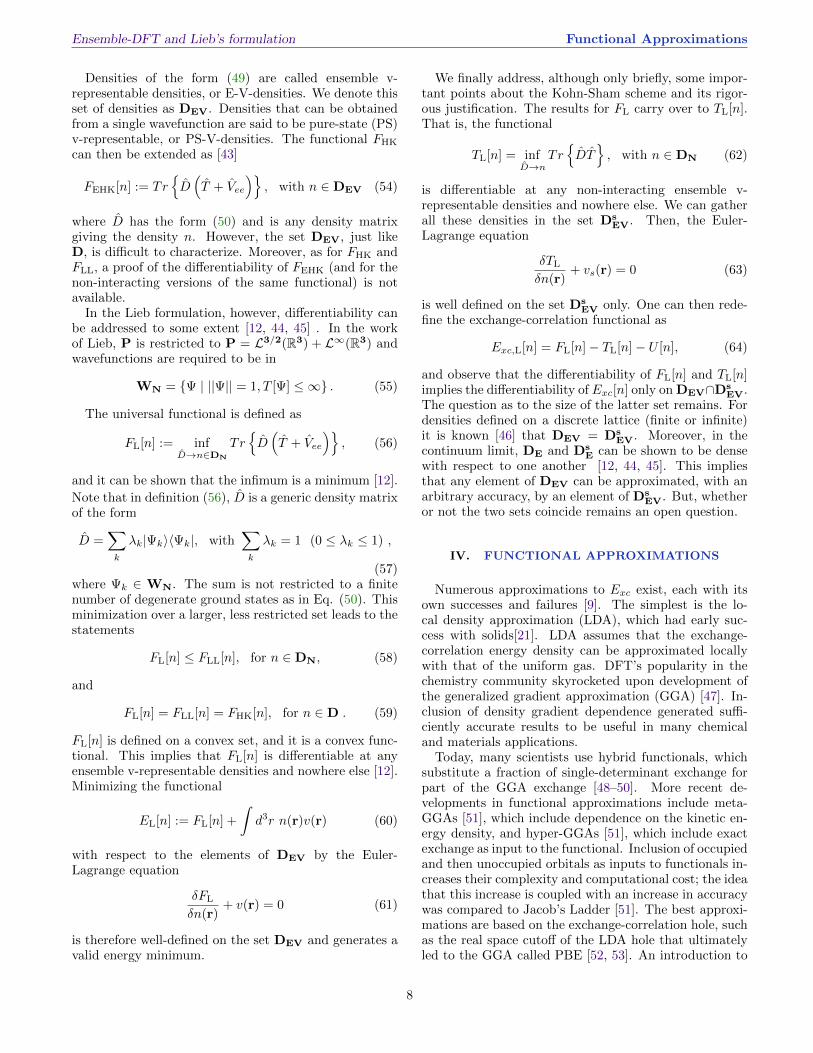
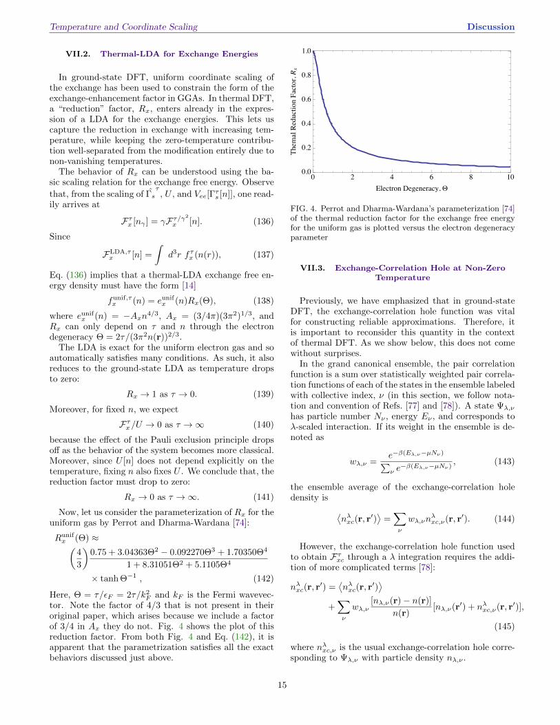
tor. Note the factor of 4/3 that is not present in theiroriginal paper, which arises because we include a factorof 3/4 in Ax they do not. Fig. 4 shows the plot of thisreduction factor. From both Fig. 4 and Eq. (142), it isapparent that the parametrization satisfies all the exactbehaviors discussed just above.

0 2 4 6 8 100.0

0.2

0.4

0.6

0.8

1.0

Electron Degeneracy, !

ThemalReductionFactor,R

x

FIG. 4. Perrot and Dharma-Wardana’s parameterization [74]of the thermal reduction factor for the exchange free energyfor the uniform gas is plotted versus the electron degeneracyparameter

VII.3. Exchange-Correlation Hole at Non-ZeroTemperature

Previously, we have emphasized that in ground-stateDFT, the exchange-correlation hole function was vitalfor constructing reliable approximations. Therefore, itis important to reconsider this quantity in the contextof thermal DFT. As we show below, this does not comewithout surprises.

In the grand canonical ensemble, the pair correlationfunction is a sum over statistically weighted pair correla-tion functions of each of the states in the ensemble labeledwith collective index, ν (in this section, we follow nota-tion and convention of Refs. [77] and [78]). A state Ψλ,ν

has particle number Nν , energy Eν , and corresponds toλ-scaled interaction. If its weight in the ensemble is de-noted as

wλ,ν =e−β(Eλ,ν−µNν)∑ν e−β(Eλ,ν−µNν)

, (143)

the ensemble average of the exchange-correlation holedensity is ⟨

nλxc(r, r′)⟩

=∑ν

wλ,νnλxc,ν(r, r′). (144)

However, the exchange-correlation hole function usedto obtain Fτxc through a λ integration requires the addi-tion of more complicated terms [78]:

nλxc(r, r′) =

⟨nλxc(r, r

′)⟩

+∑ν

wλ,ν[nλ,ν(r)− n(r)]

n(r)[nλ,ν(r′) + nλxc,ν(r, r′)],

(145)

where nλxc,ν is the usual exchange-correlation hole corre-sponding to Ψλ,ν with particle density nλ,ν .

15

Thus, the sum rule stated in the ground state getsmodified as follows [79]∫

d3r′ nλxc(r, r′) = −1 +

∑ν

wλ,νnλ,ν(r)

n(r)[Nν − 〈N〉].

(146)The last expression shows that the sum rule for thethermal exchange-correlation hole accounts for an addi-tional term due to particle number fluctuations. Worsestill, this term carries along with it state-dependent, andtherefore system-dependent, quantities. This is an im-portant warning that standard methodologies for produc-ing reliable ground-state functional approximations mustbe properly revised for use in the thermal context.

VIII. CONCLUSION

Thermal density functional theory is an area ripe fordevelopment in both fundamental theory and the con-struction of approximations because of rapidly expandingapplications in many areas. Projects underway in the sci-entific community include construction of temperature-dependent GGAs [80], exact exchange methods for non-zero temperatures [81], orbital-free approaches at non-zero temperatures [82], and continued examination of the

exact conditions that may guide both of these develop-ments [80]. In the world of warm dense matter, simu-lations are being performed, often very successfully [83],generating new insights into both materials science andthe quality of our current approximations [84]. As dis-cussed above, techniques honed for zero-temperature sys-tems should be carefully considered before being ap-plied to thermal problems. Studying exact propertiesof functionals may guide efficient progress in applicationto warm dense matter. In context, thermal DFT emergesas as a clear and solid framework that provides users anddevelopers practical and formal tools of general funda-mental relevance.

IX. ACKNOWLEDGMENTS

We would like to thank the Institute for Pure andApplied Mathematics for organization of Workshop IV:Computational Challenges in Warm Dense Matter andfor hosting APJ during the Computational Methods inHigh Energy Density Physics long program. APJ thanksthe U.S. Department of Energy (DE-FG02-97ER25308),SP and KB thank the National Science Foundation(CHE-1112442), and SP and EKUG thank EuropeanCommunity’s FP7, CRONOS project, Grant AgreementNo. 280879.

[1] N. R. C. C. on High Energy Density Plasma PhysicsPlasma Science Committee, Frontiers in High EnergyDensity Physics: The X-Games of Contemporary Science(The National Academies Press, 2003). 1

[2] T. R. Mattsson and M. P. Desjarlais, “Phase diagram andelectrical conductivity of high energy-density water fromdensity functional theory,” Phys. Rev. Lett., 97, 017801(2006). 1

[3] F. R. Graziani, V. S. Batista, L. X. Benedict, J. I. Castor,H. Chen, S. N. Chen, C. A. Fichtl, J. N. Glosli, P. E.Grabowski, A. T. Graf, S. P. Hau-Riege, A. U. Hazi, S. A.Khairallah, L. Krauss, A. B. Langdon, R. A. London,A. Markmann, M. S. Murillo, D. F. Richards, H. A. Scott,R. Shepherd, L. G. Stanton, F. H. Streitz, M. P. Surh,J. C. Weisheit, and H. D. Whitley, “Large-scale moleculardynamics simulations of dense plasmas: The CimarronProject,” High Energy Density Physics, 8, 105 (2012).

[4] K. Y. Sanbonmatsu, L. E. Thode, H. X. Vu, andM. S. Murillo, “Comparison of molecular dynamics andparticle-in-cell simulations for strongly coupled plasmas,”J. Phys. IV France, 10, Pr5 (2000). 1

[5] S. Atzeni and J. Meyer-ter Vehn, The Physics of InertialFusion: Beam-Plasma Interaction, Hydrodynamics, HotDense Matter (Clarendon Press, 2004). 1

[6] M. D. Knudson and M. P. Desjarlais, “Shock compressionof quartz to 1.6 TPa: Redefining a pressure standard,”Phys. Rev. Lett., 103, 225501 (2009). 1

[7] A. Kietzmann, R. Redmer, M. P. Desjarlais, and T. R.Mattsson, “Complex behavior of fluid lithium under ex-treme conditions,” Phys. Rev. Lett., 101, 070401 (2008).

1[8] S. Root, R. J. Magyar, J. H. Carpenter, D. L. Hanson,

and T. R. Mattsson, “Shock compression of a fifth periodelement: Liquid xenon to 840 GPa,” Phys. Rev. Lett.,105, 085501 (2010). 1

[9] K. Burke, “Perspective on density functional theory,” J.Chem. Phys., 136, 150901 (2012). 1, 2, 8

[10] P. Hohenberg and W. Kohn, “Inhomogeneous electrongas,” Phys. Rev., 136, B864 (1964). 1, 2

[11] M. Levy, “Universal variational functionals of electrondensities, first-order density matrices, and natural spin-orbitals and solution of the v-representability problem,”Proceedings of the National Academy of Sciences of theUnited States of America, 76, 6062 (1979). 1, 4, 6, 11

[12] E. H. Lieb, “Density functionals for coulomb systems,”Int. J. Quantum Chem., 24, 243 (1983). 1, 5, 6, 7, 8

[13] N. D. Mermin, “Thermal properties of the inhomogenouselectron gas,” Phys. Rev., 137, A: 1441 (1965). 2, 11

[14] S. Pittalis, C. R. Proetto, A. Floris, A. Sanna, C. Bersier,K. Burke, and E. K. U. Gross, “Exact conditions in finite-temperature density-functional theory,” Phys. Rev. Lett.,107, 163001 (2011). 2, 13, 14, 15

[15] J. W. Dufty and S. B. Trickey, “Scaling, bounds, andinequalities for the noninteracting density functionals atfinite temperature,” Phys. Rev. B, 84, 125118 (2011),interested readers should note that Dufty and Trickeyalso have a paper concerning interacting functionals inpreparation. 2, 13

[16] L. H. Thomas, “The calculation of atomic fields,” Math.Proc. Camb. Phil. Soc., 23, 542 (1927). 2, 9

16

[17] E. Fermi, Rend. Acc. Naz. Lincei, 6 (1927).[18] E. Fermi, “Eine statistische Methode zur Bestimmung

einiger Eigenschaften des Atoms und ihre Anwendungauf die Theorie des periodischen Systems der Elemente (astatistical method for the determination of some atomicproperties and the application of this method to the the-ory of the periodic system of elements),” Zeitschrift furPhysik A Hadrons and Nuclei, 48, 73 (1928). 2, 9

[19] V. Fock, “Naherungsmethode zur losung des quanten-mechanischen mehrkorperproblems,” Z. Phys., 61, 126(1930). 2

[20] D. R. Hartree and W. Hartree, “Self-Consistent Field,with Exchange, for Beryllium,” Proceedings of the RoyalSociety of London. Series A - Mathematical and PhysicalSciences, 150, 9 (1935). 2

[21] W. Kohn and L. J. Sham, “Self-consistent equations in-cluding exchange and correlation effects,” Phys. Rev.,140, A1133 (1965). 2, 8, 11

[22] K. Burke, “The ABC of DFT,” (2007), available online.2, 9

[23] K. Burke and L. O. Wagner, “DFT in a nutshell,” Int. J.Quant. Chem., 113, 96 (2013). 2

[24] F. Schwabl, Quantum Mechanics (Springer-Verlag,2007). 2

[25] J. J. Sakurai, Modern Quantum Mechanics (Revised Edi-tion) (Addison Wesley, 1993). 2

[26] E. Engel and R. M. Dreizler, Density Functional Theory:An Advanced Course (Springer–Verlag, 2011). 3, 6, 7, 13

[27] C. D. Sherrill, “Frontiers in electronic structure theory,”The Journal of Chemical Physics, 132, 110902 (2010). 3

[28] R. M. Dreizler and E. K. U. Gross, Density FunctionalTheory: An Approach to the Quantum Many-Body Prob-lem (Springer–Verlag, 1990). 3, 4, 7, 9

[29] W. Kohn, in Highlight of Condensed Matter Theory,edited by F. Bassani, F. Fumi, and M. P. Tosi (North-Holland, Amsterdam, 1985) p. 1. 4

[30] G. F. Giuliani and G. Vignale, eds., Quantum Theory ofthe Electron Liquid (Cambridge University Press, 2008).4, 7

[31] R. Dreizler, J. da Providencia, and N. A. T. O. S. A. Di-vision, eds., in “Density functional methods in physics,”, NATO ASI B Series (Springer Dordrecht, 1985). 5

[32] H. Englisch and R. Englisch, “Hohenberg-Kohn theoremand non-V-representable densities,” Physica A: Statisti-cal Mechanics and its Applications, 121, 253 (1983). 5

[33] F. W. Averill and G. S. Painter, Phys. Rev. B, 15, 2498(1992). 5

[34] S. G. Wang and W. H. E. Scharz, J. Chem. Phys., 105,4641 (1996).

[35] P. R. T. Schipper, O. V. Gritsenko, and E. J. Baerends,Theor. Chem. Acc., 99, 4056 (1998).

[36] P. R. T. Schipper, O. V. Gritsenko, and E. J. Baerends,J. Chem. Phys., 111, 4056 (1999).

[37] C. A. Ullrich and W. Kohn, “Kohn-sham theory forground-state ensembles,” Phys. Rev. Lett., 87, 093001(2001). 5

[38] M. Reed and B. Simon, I: Functional Analysis (Meth-ods of Modern Mathematical Physics) (Academic Press,1981). 6

[39] J. Harriman, Phys. Rev. A, 24, 680 (1981). 7[40] R. G. Parr and W. Yang, Density Functional Theory of

Atoms and Molecules (Oxford University Press, 1989). 7,11

[41] R. van Leeuwen, Adv. in Q. Chem., 43, 24 (2003). 7

[42] M. Levy, Phys. Rev. A, 26, 1200 (1982). 7[43] S. V. Valone, J. Chem. Phys., 73, 1344 (1980). 8[44] H. Englisch and R. Englisch, Phys. Stat. Solidi B, 123,

711 (1984). 8[45] H. Englisch and R. Englisch, Phys. Stat. Solidi B, 124,

373 (1984). 8[46] J. T. Chayes, L. Chayes, and M. B. Ruskai, J. Stat. Phys,

38, 497 (1985). 8[47] J. Perdew, “Density functional approximation for the

correlation energy of the inhomogeneous gas,” Phys. Rev.B, 33, 8822 (1986). 8

[48] A. D. Becke, “Density-functional exchange-energy ap-proximation with correct asymptotic behavior,” Phys.Rev. A, 38, 3098 (1988). 8

[49] A. D. Becke, “Density-functional thermochemistry. iii.the role of exact exchange,” The Journal of ChemicalPhysics, 98, 5648 (1993).

[50] C. Lee, W. Yang, and R. G. Parr, “Development ofthe Colle-Salvetti correlation-energy formula into a func-tional of the electron density,” Phys. Rev. B, 37, 785(1988). 8

[51] J. P. Perdew and K. Schmidt, in Density Functional The-ory and Its Applications to Materials, edited by V. E. V.Doren, K. V. Alsenoy, and P. Geerlings (American Insti-tute of Physics, Melville, NY, 2001). 8

[52] J. P. Perdew, K. Burke, and M. Ernzerhof, “Generalizedgradient approximation made simple,” Phys. Rev. Lett.,77, 3865 (1996), ibid. 78, 1396(E) (1997). 8, 10

[53] J. Perdew, K. Burke, and M. Ernzerhof, “Perdew, Burke,and Ernzerhof reply,” Phys. Rev. Lett., 80, 891 (1998).8

[54] V. V. Karasiev, R. S. Jones, S. B. Trickey, and F. E.Harris, “Properties of constraint-based single-point ap-proximate kinetic energy functionals,” Phys. Rev. B, 80,245120 (2009). 9

[55] V. V. Karasiev, R. S. Jones, S. B. Trickey, and F. E.Harris, “Erratum: Properties of constraint-based single-point approximate kinetic energy functionals [phys. rev.b 80, 245120 (2009)],” Phys. Rev. B, 87, 239903 (2013).

[56] V. Karasiev and S. Trickey, “Issues and challenges inorbital-free density functional calculations,” ComputerPhysics Communications, 183, 2519 (2012).

[57] Y. A. Wang and E. A. Carter, in Theoretical Methods inCondensed Phase Chemistry, edited by S. D. Schwartz(Kluwer, Dordrecht, 2000) Chap. 5, p. 117. 9

[58] J. C. Snyder, M. Rupp, K. Hansen, K.-R. Mueller, andK. Burke, “Finding density functionals with machinelearning,” Phys. Rev. Lett., 108, 253002 (2012). 9

[59] M. Levy and J. Perdew, “Hellmann-Feynman, virial, andscaling requisites for the exact universal density function-als. shape of the correlation potential and diamagneticsusceptibility for atoms,” Phys. Rev. A, 32, 2010 (1985).9

[60] J. P. Perdew and S. Kurth, in A Primer in Density Func-tional Theory, edited by C. Fiolhais, F. Nogueira, andM. A. L. Marques (Springer, Berlin / Heidelberg, 2003)pp. 1–55. 9, 10

[61] O. Gunnarsson and B. Lundqvist, “Exchange and corre-lation in atoms, molecules, and solids by the spin-density-functional formalism,” Phys. Rev. B, 13, 4274 (1976). 9

[62] D. Langreth and J. Perdew, “The exchange-correlationenergy of a metallic surface,” Solid State Commun., 17,1425 (1975). 9

17

[63] M. Ernzerhof, K. Burke, and J. P. Perdew, in Recent De-velopments and Applications in Density Functional The-ory, edited by J. M. Seminario (Elsevier, Amsterdam,1996). 10

[64] R. Jones and O. Gunnarsson, “The density functionalformalism, its applications and prospects,” Rev. Mod.Phys., 61, 689 (1989). 10

[65] K. Burke, J. Perdew, and D. Langreth, “Is the local spindensity approximation exact for short-wavelength fluctu-ations?” Phys. Rev. Lett., 73, 1283 (1994). 10

[66] A. C. Cancio, C. Y. Fong, and J. S. Nelson, “Exchange-correlation hole of the Si atom: A quantum Monte Carlostudy,” Phys. Rev. A, 62, 062507 (2000). 10

[67] H. Eschrig, “T > 0 ensemble-state density functional the-ory via Legendre transform,” Phys. Rev. B, 82, 205120(2010). 10

[68] A. Theophilou, “The energy density functional formalismfor excited states,” J. Phys. C, 12, 5419 (1979). 12

[69] E. Gross, L. Oliveira, and W. Kohn, “Density-functionaltheory for ensembles of fractionally occupied states. i.basic formalism,” Phys. Rev. A, 37, 2809 (1988). 12

[70] L. Oliveira, E. Gross, and W. Kohn, “Density-functionaltheory for ensembles of fractionally occupied states. ii.application to the helium atom,” Phys. Rev. A, 37, 2821(1988).

[71] A. Nagy, “Kohn-sham equations for multiplets,” Phys.Rev. A, 57, 1672 (1998). 12

[72] N. I. Gidopoulos, P. G. Papaconstantinou, and E. K. U.Gross, “Spurious interactions, and their correction, in theensemble-kohn-sham scheme for excited states,” Phys.Rev. Lett., 88, 033003 (2002). 12

[73] F. Perrot, “Gradient correction to the statistical elec-tronic free energy at nonzero temperatures: Applicationto equation-of-state calculations,” Phys. Rev. A, 20, 586(1979). 14

[74] F. Perrot and M. W. C. Dharma-wardana, “Exchangeand correlation potentials for electron-ion systems at fi-

nite temperatures,” Phys. Rev. A, 30, 2619 (1984). 15[75] F. Perrot and M. W. C. Dharma-wardana, “Spin-

polarized electron liquid at arbitrary temperatures:Exchange-correlation energies, electron-distributionfunctions, and the static response functions,” Phys. Rev.B, 62, 16536 (2000).

[76] R. G. Dandrea, N. W. Ashcroft, and A. E. Carlsson,“Electron liquid at any degeneracy,” Phys. Rev. B, 34,2097 (1986). 14

[77] J. Perdew, in Density Functional Method in Physics,vol. 123 of NATO Advanced Study Institute, Series B:Physics, edited by R. Dreizler and J. da Providencia(Plenum, New York, 1985). 15

[78] S. Kurth and J. P. Perdew, in Strongly Coupled CoulombSystems, edited by G. J. Kalman, J. M. Rommel, andK. Blagoev (Plenum Press, New York, NY, 1998). 15

[79] J. P. Perdew, “Density functional theory and the band-gap problem,” International Journal Of Quantum Chem-istry, 28, 497 (1985). 16

[80] A. Pribram-Jones, S. Pittalis, and K. Burke, (TBD), inpreparation. 16

[81] M. Greiner, P. Carrier, and A. Gorling, “Extension ofexact-exchange density functional theory of solids to fi-nite temperatures,” Phys. Rev. B, 81, 155119 (2010). 16

[82] V. V. Karasiev, T. Sjostrom, and S. B. Trickey,“Generalized-gradient-approximation noninteractingfree-energy functionals for orbital-free density functionalcalculations,” Phys. Rev. B, 86, 115101 (2012). 16

[83] K.-U. Plagemann, P. Sperling, R. Thiele, M. P. Desjar-lais, C. Fortmann, T. Doppner, H. J. Lee, S. H. Glen-zer, and R. Redmer, “Dynamic structure factor in warmdense beryllium,” New Journal of Physics, 14, 055020(2012). 16

[84] A. Pribram-Jones, S. Pittalis, and K. Burke, (TBD), inpreparation. 16

18