Thermal comfort in residential buildings: Comfort valuesand scales for building energy simulationPeeters, L.F.R.; Dear, de, R.; Hensen, J.L.M.; D'Haeseleer, W.

Published in:Applied Energy

DOI:10.1016/j.apenergy.2008.07.011

Published: 01/01/2009

Document VersionAccepted manuscript including changes made at the peer-review stage

Please check the document version of this publication:

• A submitted manuscript is the author's version of the article upon submission and before peer-review. There can be important differencesbetween the submitted version and the official published version of record. People interested in the research are advised to contact theauthor for the final version of the publication, or visit the DOI to the publisher's website.• The final author version and the galley proof are versions of the publication after peer review.• The final published version features the final layout of the paper including the volume, issue and page numbers.

Link to publication

Citation for published version (APA):Peeters, L. F. R., Dear, de, R., Hensen, J. L. M., & D'Haeseleer, W. (2009). Thermal comfort in residentialbuildings: Comfort values and scales for building energy simulation. Applied Energy, 86(5), 772-780. DOI:10.1016/j.apenergy.2008.07.011

General rightsCopyright and moral rights for the publications made accessible in the public portal are retained by the authors and/or other copyright ownersand it is a condition of accessing publications that users recognise and abide by the legal requirements associated with these rights.

• Users may download and print one copy of any publication from the public portal for the purpose of private study or research. • You may not further distribute the material or use it for any profit-making activity or commercial gain • You may freely distribute the URL identifying the publication in the public portal ?

Take down policyIf you believe that this document breaches copyright please contact us providing details, and we will remove access to the work immediatelyand investigate your claim.

Download date: 04. Jun. 2018

1.1

Thermal comfort in residential buildings: comfort values and scales for

building energy simulation.

Leen Peeters1,a

, Richard de Dearb, Jan Hensen

c, William D‟haeseleer

*,a

a Division of Applied Mechanics and Energy Conversion, University of Leuven (K.U.Leuven),

Celestijnenlaan 300A / B-3001 Leuven / Belgium

b Division of Environmental and Life Sciences, Macquarie University, Sydney, Australia

c Faculty of Architecture, Building and Planning, Technische Universiteit Eindhoven, Vertigo 6.18, P.O.

Box 513, 5600 MB Eindhoven, The Netherlands

Abstract

Building Energy Simulation (BES) programmes often use conventional thermal comfort

theories to make decisions, whilst recent research in the field of thermal comfort clearly

shows that important effects are not incorporated. The conventional theories of thermal

comfort were set up based on steady state laboratory experiments. This, however, is not

representing the real situation in buildings, especially not when focusing on residential

buildings. Therefore, in present analysis, recent reviews and adaptations are considered

to extract acceptable temperature ranges and comfort scales. They will be defined in an

algorithm, easily implementable in any BES code. The focus is on comfortable

Correspondence to: William D‟haeseleer, Division of Applied Mechanics and Energy Conversion,

University of Leuven (K.U.Leuven), Celestijnenlaan 300 A, B-3001 Leuven, Belgium

Phone +32/16/32.25.11 Fax. +32/16/32.29.85

E-mail: william.dhaeseleer@mech.kuleuven.be

1 E-mail: l.f.r.peeters@gmail.com

1.2

temperature levels in the room, more than on the detailed temperature distribution

within that room.

Keywords: comfort temperatures, residential buildings, adaptation, temperature ranges

1. . Introduction

When comparing the effect of changes to buildings, either changes to the building

structure, the materials used or the installations, an important boundary condition is that

the thermal comfort quality must, in all cases, be maintained. Building Energy

Simulation codes often use conventional methods to determine the achieved comfort

level: common codes as ESP-r [1], TRNSYS [2] and IDA Ice [3] use the ISO 7730

assessment method. However, when focusing on residential buildings, including zones

with variable thermal comfort requirements, less predictable activities and more ways to

adapt to the existing thermal environment, the conventional methods are no longer

satisfactory. Comfort temperatures as well as acceptable temperature variations are

more influenced by parameters not considered by the conventional methods. Therefore,

algorithms for determination of the neutral or comfort temperatures in the different

zones of a residential building, as well as for the estimation of the thermal sensation of

the building occupants in these zones, will improve the resemblance with reality. These

algorithms must take into account the knowledge of the traditional methods as well as

recent findings in the field of thermal comfort with a focus on residential buildings.

1.3

2. . Conventional Models of Thermal Comfort

2.1. Fanger’s approach

In order to develop mathematical models to predict people‟s responses on the thermal

quality of an environment, researchers have been exploring the thermal, physiological

and psychological response of people in varying circumstances. „Thermal comfort‟ is

defined as “that condition of mind which expresses satisfaction with the thermal

environment” [4]. Thermal comfort is a result of a combination/adaptation of

parameters of both the environment and the human body itself. Fanger, who developed

the first heat balance thermal comfort model [5], stated that the condition for thermal

comfort is thus that skin temperature and sweat secretion lie within narrow limits. For

his comfort equation, Fanger obtained data from climate chamber experiments, during

which sweat rate and skin temperature were measured on people who judged their

thermal sensation as comfortable. He then defined an estimation of skin temperature and

sweat secretion as a function of metabolic rate by regression analyses of the measured

data. This way, an expression for optimal thermal comfort can be deduced from the

metabolic rate, clothing insulation and environmental conditions. His assumption for

this was that the sensation experienced by a person is a function of the physiological

strain imposed on him by the environment. The thermal environment is taken into

account by the air temperature, the mean radiant temperature, the partial pressure of

water vapour in ambient air and the air velocity.

Satisfying of the comfort equation is a condition for optimal thermal comfort. It,

however, only gives information on the possible combination of the variables to achieve

1.4

thermal comfort. Additionally, Fanger proposed a method to predict the actual thermal

sensation of persons in an arbitrary climate where the variables might not satisfy the

equation: the Predicted Mean Vote (PMV). This, he defined as "the difference between

the internal heat production and the heat loss to the actual environment for a man kept at

the comfort values for skin temperature and sweat production at the actual activity

level". Following Fanger then, the sensation of thermal comfort is quantified by an

adapted ASHRAE 7-point psycho-physical scale with values ranging from -3, indicating

cold, over 0, indicating neutral, to +3, indicating hot. With experiments in a constant,

well controlled, environment, Fanger obtained a reasonable statistical basis for the

quantification of his PMV-index. The method allows to predict what comfort vote

would arise from a large group of individuals for a given set of environmental

conditions for a given clothing insulation and metabolic rate.

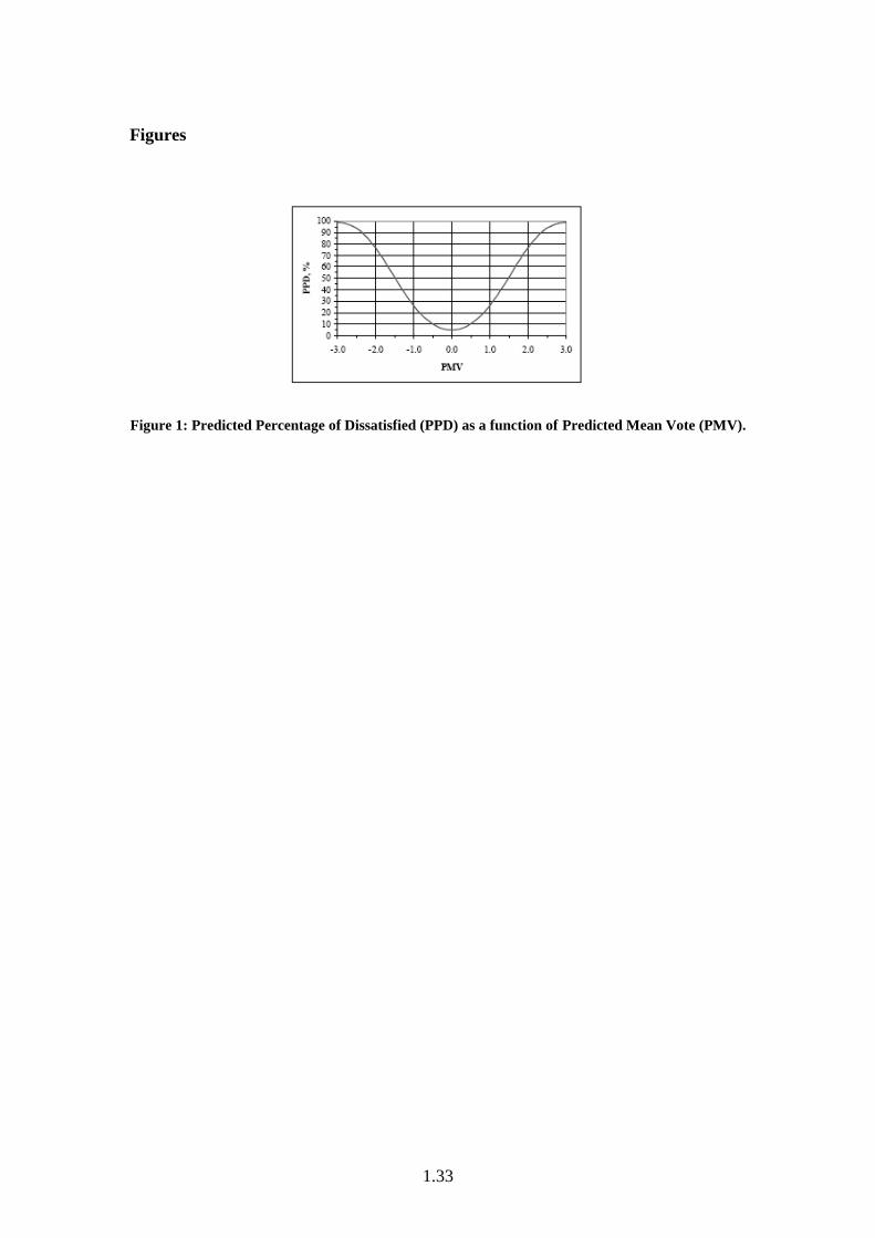
It nevertheless might be more meaningful to state what percentage of persons can be

expected to be dissatisfied, because that indicates the number of potential complainers.

The dissatisfied are defined as those voting outside the range of -1 (slightly cool) to +1

(slightly warm). Through steady state experiments, Fanger determined the relationship

between the PMV-index and the Predicted Percentage of Dissatisfied (PPD), as shown

in Figure 1. This figure shows a PPD of 5% for a PMV equal to 0. That indicates the

impossibility to satisfy all persons in a large group sharing a collective climate.

Complaints cannot be avoided, but should be kept to the minimum as shown in Figure

1.

The curve of Figure 1 shows an equal amount of complaints on the „warm‟ side as on

the „cold‟ side: the curve is symmetric around the PMV of 0. At the optimal condition,

1.5

there is thus a balance between those sensing uncomfortably warm and those sensing

uncomfortably cold. However, a deviation from 0 would not only mean a greater

percentage of dissatisfied, but also an asymmetric distribution between those

experiencing warmth and those experiencing cold. This is expected to result in a

demand for a unilateral change.

2.2. International Standards on thermal comfort

The International Standard ISO 7730 [6] uses these PMV and PPD indeces to predict

the thermal sensation of people exposed to moderate thermal environments, as well as to

specify acceptable thermal environmental conditions for comfort. Local discomfort and

draught are taken into account by additional conditions. As it is not known whether or

how the number of dissatisfied due to local discomfort can be added to those dissatisfied

due to general thermal discomfort, or whether the percentage of the total dissatisfied

equals the sum of the dissatisfied per individual discomfort criterion, the ISO 7730

proposes to specify different levels of comfort [7]. The optimal temperature is the same

for the different comfort classes, but the acceptable temperature range will vary as the

allowed percentage of dissatisfied changes. The limits of validity for different variables,

whether included in the equations or not, are listed for each comfort level. It is stated

that the standard applies to indoor environments where steady state thermal comfort or

moderate deviations from comfort occur. When considering thermal environments in

which occupants have many possibilities to adapt themselves or the environment to

achieve a more agreeable thermal sensation, the ISO standard suggests using a wider

PMV range.

1.6

The standard 55-2004 set up by ASHRAE [4] is a revision of the former ASHRAE 55-

1992. As the ISO 7730, also the ASHRAE 55 is valid for healthy, adult people. The

activities they perform, the clothes they wear and the thermal environment they occupy,

all are determined by variable values within given limits. Besides the recommended

PPD and PMV ranges, this standard increases the percentage of persons dissatisfied

with 10 percent points, to incorporate the effect of local thermal discomfort, e.g. draft

and temperature asymmetry. It also determines the values of acceptable temperature

changes per given time interval. Thereby partly accounting for the dynamic effects

ignored both by Fanger [5] and in ISO 7730 [6].

2.3. Remarks on current methods

The PMV and PPD concepts were derived based on steady state laboratory experiments,

with in most cases test persons wearing standardized uniforms executing sedentary

activities. Numerous publications assess this steady state approach as a failure

([8],[9],[10],[11]). Another often mentioned input error has to do with the correct

estimation or determination of the insulation of the clothing garments or ensembles

([8],[12]) and the sensitivity of the PMV equation to this [11].

The majority of comments is on PMV or PPD disregarding the effect of adaptation.

Adaptation in this context is the changing evaluation of the thermal environment

because of changing perceptions. Different forms of adaptation can be distinguished,

which are connected and will influence one another ([12],[13]).

Psychological adaptation depends on experiences, habituations and expectations

of the indoor environment ([14],[15],[16]).

1.7

Physiological adaptation can be broken down into two major subcategories:

genetic adaptation and acclimatization. The former deals with effects on timescales

beyond that of an individual‟s lifetime. The latter comprehends changes in the settings

of the physiological thermoregulation system over a period of a few days or weeks. It is

the response to sustained exposure to one or more thermal environmental stressors [12].

Behavioural thermoregulation, or adjustment, includes all modifications a

person might consciously or unconsciously make, which in turn modify heat and mass

fluxes governing the body‟s thermal balance [12]: personal adjustment ([11],[17],[18]),

technological or environmental adjustment [4] and cultural adjustment.

3. . Residential buildings

3.1. General considerations

Focusing on residential buildings, conditions are not quite comparable to those during

the experiments for calibration of the PMV and PPD equations. The domestic scene is

far from steady state: both the activity level2 and the clothing value

3 can vary within

small timescales, fluctuating internal gains can rapidly affect the indoor temperature and

the variation in occupancy will influence, amongst others, the required ventilation rate.

Nearly all forms of adaptations apply to the case of residential buildings: changing

activity, clothing, opening windows, drinking cold or warm drinks, expected

temperatures in summer, siestas, etc..

2 The activity level indicates the intensity of the physical action of a person. The dimension met is used to

express the consequently generated energy inside the body.1 met equals 58.2 W/m2, the energy produced

per surface area of an average person at rest. 3 The clothing factor is the total thermal resistance from the skin to the outer surface of the clothed body.

However it is dimensionless, it is common to indicate it in clo.

1.8

Calculation of the indoor comfort temperature, being the most important environmental

parameter [19] of a residential building, thus should incorporate the effects of

adaptation. Based on the above gathered knowledge, some common methods are

compared and discussed, focusing on residential buildings.

In this paper, 3 thermal zones are distinguished in residential buildings: bathroom,

bedroom and others. In bathrooms, a wet naked body requires special thermal comfort,

while in a bedroom especially overheating requires attention. Other zones include

mainly kitchen, living room and office, in which mostly the activity levels are rather

low (0.7 met for reclining to 2.0 met for cooking [4]) and the clothing is in accordance with

outdoor conditions.

3.2. Temperature characterization

To incorporate the adaptation to the outdoor climate, influencing more than just the

clothing ([18],[20],[21],[22]), the outdoor temperature must be characterized by a value

that includes the required amount of detail. It is clear that the effect of the detailed

course of the external temperature will partly be flattened out by the time constants of

the building. When averaging information over a long period, however, some effects

risk to be neglected. Some methods use monthly averaged external temperature values,

while amongst others Humphreys et al. suggest that most adaptation is within a week or

so [20]. Morgan and de Dear demonstrate that besides today‟s weather also the weather

of yesterday and that of the past few days influence clothing and perception of comfort

temperature [23]. An appropriate measure for the incorporation of the outdoor

1.9

temperature is therefore required, so that it can respond to the day to day weather

variations.

In Van der Linden et al, the adaptive temperature limits (ATL) method is defined for the

Dutch official purposes [24], using Te,ref;

1 2 3

,

( 0.8 0.4 0.2 )

2.4

today today today today

e ref

T T T TT

(1)

where ,e refT = reference external temperature (in °C)

todayT = arrhythmic average of today‟s maximum and minimum external temperature

(°C)

1todayT = arrhythmic average of yesterday‟s maximum and minimum external

temperature (°C)

2todayT = arrhythmic average of maximum and minimum external temperature of 2 days

ago (°C)

3todayT = arrhythmic average of maximum and minimum external temperature of 3 days

ago (°C).

That method has been set up to be used in different building types. However, it must be

interpreted with care when the focus is on special zones such as bathrooms and

bedrooms. In case of rooms with office-like activity levels and clothing values varying

from 0.5 to 2.0 clo (including added values to account for the effect of chairs or sofas),

it can be used for a residential context as well. Also Nicol and McCartney have set up a

short term relationship for activity levels and clothing values in the same range [25]. In

task 3 of their SCATS project, they developed an adaptive algorithm for comfort

1.10

temperatures in terms of outdoor temperature. It resulted in the following equation for

incorporating the outdoor temperature [26]:

1 1(1 )n n n

RM RM DMT cT c T (2)

where n

RMT = mathematical daily average temperature on day „n‟ in °C

1n

RMT = mathematical daily average temperature on day „n-1‟ in °C

1n

DMT = mathematical daily average temperature on day „n-1‟ in °C

c = a constant.

The constant was derived from empirical field study data in offices and public buildings

in different European countries, resulting in a value of 0.8. The format of equation (2)

does express a short term relation with the external conditions.

In the ATL method, more emphasis is given on more recent weather data, as can be seen

by comparing equation (1) with the elaborated equation of n

RMT , given by equation (3):

1 2 3 40.2 0.16 0.128 0.1024 ....n n n n n

RM DM DM DM DMT T T T T (3)

As the literature shows that also the current outdoor condition is of importance

([27],[28]), the ATL-calculation, ,e refT , is preferred. The difference will, however, be

small in cases of moderate climates. The ease of implementation in a particular BES

code might therefore be decisive.

1.11

3.3. The three different zones

3.3.1. Bathroom

The bathroom has a critical lower limit defined as the coldest temperature that is

acceptable to a nude, wet body. However, once dry and dresses the person must still feel

comfortable. A similar wide range of wet, nude and dressed persons in the same zone

can be found in a swimming pool. Lammers [29] describes this situation, indicating

three groups of occupants: the drying swimmers (person with skin wetness of 20%), the

superintendent and the spectators. Seven male persons showering and drying afterwards,

were tested on skin temperature and evaporative losses. Lammers ends up with comfort

operative temperature values between 21°C and 30.5°C. Similar values, especially

focused on bathrooms, can be found in Tochihara et al. [30] and Zingano [31]. The

former tested 12 male students ending up with values between 22°C and 30°C. The

latter provided 20 families with thermometers leading to 275 data points, with a neutral

temperature of 24.6°C.

As the condition of being wet and uncovered is limited in time, is taken into account to

define the upper limit of the comfort temperature band. In most cases, the body will

either be covered, or uncovered but dry. The same accounts for the raise in relative

humidity: both the occasions and their duration are limited as bathrooms are used for

more than bathing. The comfort temperature will thus be influenced by the seasonal

dependent clothing (either nightwear, either daywear) and the metabolic rate of the

performed tasks.

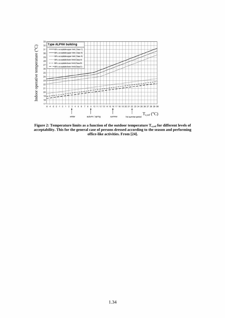
The adaptive temperature limits defined by Van der Linden, et al., for different building

types, are shown in Figure 2 [24], where ,e refT is given by the above stated equation (1).

1.12

The method is set up for so called alpha and beta buildings. Residential buildings are

considered as alpha type buildings, i.e. buildings in which occupants can make many

adaptations, including operable windows. Beta buildings will have limited adaptive

opportunities and mostly sealed facades [32].

Tochihara et al., focusing specifically on bathrooms, conclude the 90% acceptability

range for wet and/or naked people to be between 24°C to 28°C [30]. They therefore

compared their test results with the values they found in various literature sources.

Comparing this with the results of Van der Linden et al. in Figure 2, where the

conclusions are set up with clothing values according to the season, the acceptable

values for wet and/or naked persons are even above the 80% acceptability range of the

dressed bodies for cold days. Evolving to the 80% acceptability limit for both situations,

results in a compromise for the comfort temperature that is presented by the upper limit

of the 80% acceptability range of Figure 2. Therefore, in this paper, the following

equations for the neutral temperatures Tn (°C) have been derived:

,0.112 22.65n e refT T C for , 11e refT C (4)

,0.306 20.32n e refT T C for , 11e refT C (5)

3.3.2. Bedrooms

The theoretical analysis of Maeyens et al. [33] describes the effect of a decreasing body

temperature and metabolism on summer comfort temperatures in bedrooms.

Considering the calculation of the neutral or comfort temperature with any heat balance

model, this would result in higher comfort temperatures. The authors however, mention

1.13

the absence, also described in other works, of adaptation to low or high temperatures in

bedrooms. According to Maeyens et al., the explanation offered by Parmeggiani is that

physiological and behavioural adaptation is limited during sleep.

Maeyens et al. suggest using the equation of Fanger to calculate the comfort or neutral

temperature and define the input parameters as:

- Metabolic rate of sleeping: 0.7 met

- Clothing index (sleepwear, sheets, mattress and pillow): 0.8 clo

- Relative humidity: 55%

- Air speed: 0.05 to 1 m/s

That the Fanger equation cannot be applied in all cases has been clearly explained

above. Therefore, the validity of this equation is checked comparing the above stated

parameter values with the results of the parametric analyses as given in [9]. These last

authors define for each variable a range of application, more restricted than what is

given in ISO 7730. It turns out that all parameter estimates of Maeyens et al. meet even

the 90% acceptability requirements, except for the metabolic rate, being just under

Humpreys and Nicols‟ suggested lower limit of 0.8 met. A value of 0.7 met however,

still results in a level B comfort rating and is thus acceptable.

Applying the Fanger equation with these assumptions results in a summer comfort

temperature estimate of 26.4° C, with a maximum of 27.5°C (PMV +0.5). This is close

to the maximum temperature of 26°C suggested by CIBSE [34]. CIBSE shows the

results of data collected in the UK by Humphreys [35], indicating the quality of sleep as

a function of the bedroom temperature. A steep drop in quality can be seen for bedroom

temperatures above 24°C. Both this CIBSE Guide A, as well as the ASHRAE 55-2004

1.14

indicate that higher bedroom temperatures can be accepted if a fan is used: ASHRAE

indicates an acceptable increase of up to 3°C.

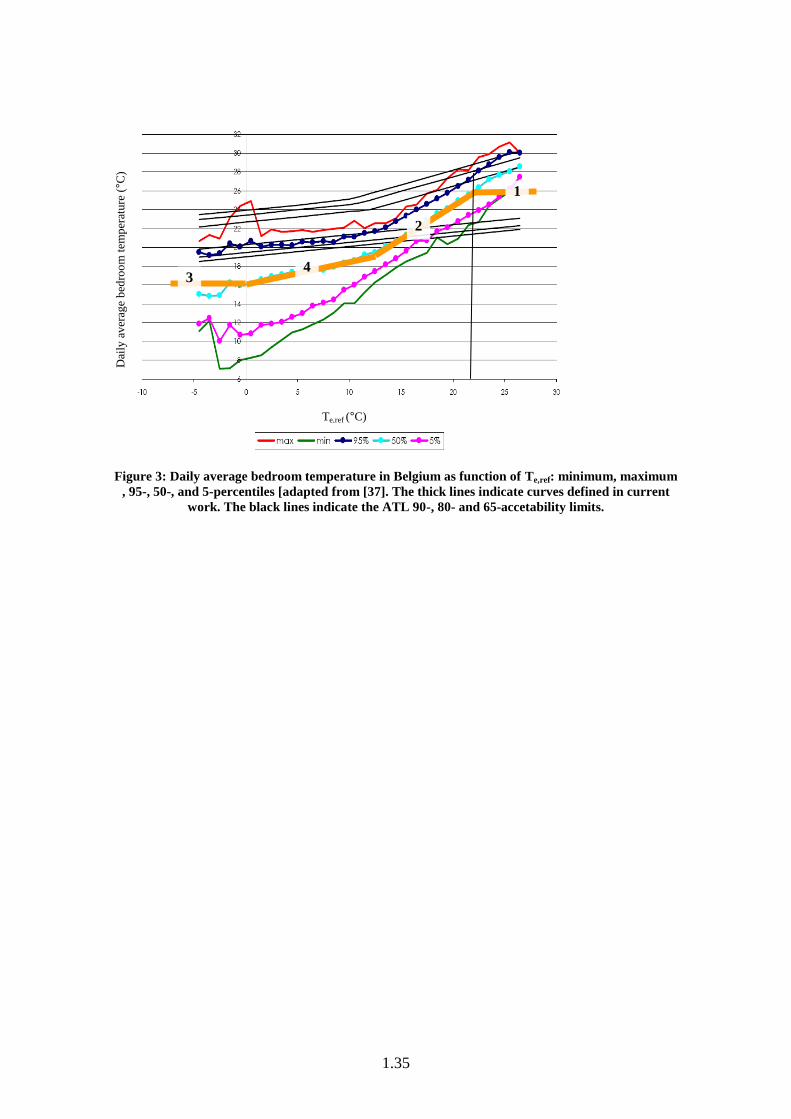
Figure 3 shows the bedroom temperatures in a recent monitoring campaign in 39

Belgian houses, where monitoring periods varied from 6 months to 2 years ([36],[37]).

The daily mean bedroom temperature is shown as a function of Te,ref (as introduced in

equation (1) above). The aim of the research was not to investigate thermal comfort,

therefore it should be interpreted with care.

Based on a questionnaire survey for indoor thermal sensations during summer

conditions in general, Maeyens et al. found up to 50% of respondents complained about

uncomfortably warm bedrooms (comparable with a PMV of 1 or more) [33]. This in

fact highlights the contrast between the summer comfort temperature he calculated (i.e.

26.4°C) and the observations shown in Figure 3, where only a minority had a ventilation

system. The average of the measurements below the 50-percentile curve is therefore

considered in this paper as representing the neutral temperature for summer conditions,

indicated by the thick line 1 in Figure 3. However, the value of 26°C, indicated by

CIBSE as the limit in the absence of an elevated air speed, is set here as the upper limit

in current research. It is indicated by the thick line 2 in Figure 3.

The winter temperature range for bedrooms, indicated by CIBSE, is 17°C [34].

Clalkley and Cater [38] indicate comfort temperatures of 15 to 17°C, but they do not

give any reference for that. Humphreys [35] shows with his measurements in dwellings

good sleep quality, even for bedroom temperatures as low as 12°C. However, Collins

[39] and Hartley [40] indicate the World Health Organisation‟s bedroom temperature

1.15

limit of 16°C, because of a decreasing resistance to respiratory infections once below

this temperature.

For the heating season, a strong correlation exist between the temperatures of the

bedrooms also used for other activities (e.g. watching TV, homework, etc.) and the

living room temperature. These bedrooms, requiring comfort temperatures in

accordance to the activity level and clothing value during these activities, are

represented by the 95-percentile curve in Figure 3 ([41],[42]), almost equal to the

median of the living room temperatures, measured during the same monitoring

campaign, at least for the heating season days with mean outdoor temperatures below 15

°C (as shown in Figure 4 below). The other bedrooms, used for sleeping only, are often

not heated, in some cases resulting in cold to very cold conditions.

The course of the bedroom‟s neutral temperature, as a function of the outdoor

temperature, will therefore differ from the shape shown in Figure 2: the comfort

bedroom temperature is limited in both summer and winter conditions. The above

defined upper limit as defined by Maeyens et al. will be taken for the summer estimate,

while in this paper the WHO value of 16°C will be accepted as minimum of the neutral

temperature for winter conditions (indicated by the thick line 3 in Figure 3). According

to the 50-percentile curve, this corresponds to reference outdoor temperatures of 0°C

and lower. For somewhat warmer ambient conditions, the 50-percentile curve (thick line

4 in Figure 3) defines the trend, as was the case for summer conditions. The slope of

these percentiles, however, for cold versus warm conditions being different. The

intersection of the two curves is calculated at a reference outdoor temperature of

12.6°C.

1.16

For the case of no elevated air velocity in summer, the here derived equations are given

by:

16nT C for , 0e refT C (6)

,0.23 16n e refT T for ,0 12.6e refC T C (7)

,0.77 9.18n e refT T C for ,12.6 21.8e refC T C (8)

26nT C for , 21.8e refT C (9)

3.3.3. Other rooms

Kitchen, living room and study have physical activity levels comparable to those in

offices, or just slightly more intensive: reclining, reading the newspaper, cooking etc.

have metabolic rates in the range of 0.8 met to 1.4 met, comparable to office or general

laboratory work. More adaptive options, however, are available (changing activity,

going to another room, drinking cold or warm drinks, changing garments -absence of

dress codes-, opening windows and doors for ventilation and cooling, etc). The neutral

temperature can therefore be more dependent on the outside climate than what is

generally accepted in offices.

In the SCATS project [25], Nicol and McCartney developed an adaptive algorithm for

comfort temperatures in terms of outdoor temperature. The relationships are based on

empirical field study data of offices and public buildings in different European

countries. The study included both naturally ventilated and air conditioned buildings, as

1.17

well as buildings equipped with mixed systems. Their equations indicate, by a constant

comfort temperature for lower external temperatures and an increasing comfort

temperature for increasing ambient temperatures, that occupants are less adaptive to

cold than to heat, in agreement with Jokl and Kabele [11] and the observations in

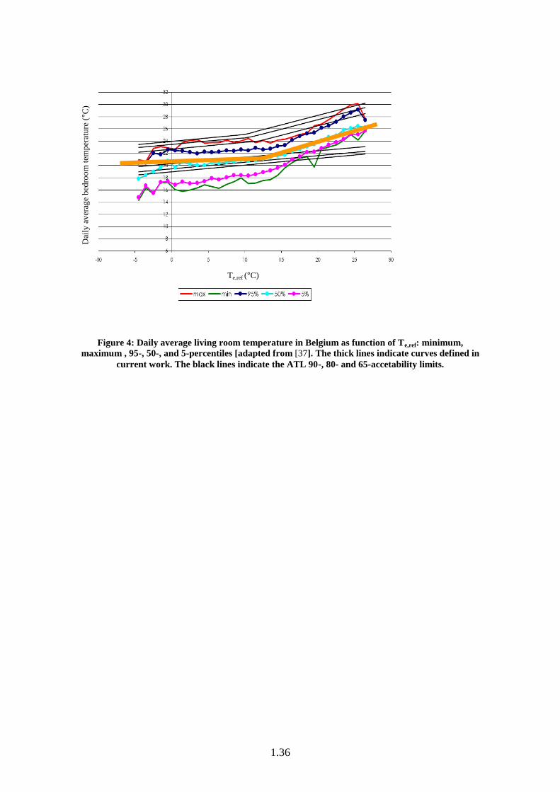
Belgian dwellings as shown in Figure 4. This is also confirmed by the ATL-method as

the slope of the comfort ranges for the alpha buildings is less steep in colder outdoor

conditions than that for warm weather; as can be seen Figure 2 and also indicated in

Figure 4. As the ATL-curve is set up with data for non-air-conditioned buildings, it is in

fact better dealing with the presence of more adaptive possibilities.

Humphreys and Hancock [14] mention that temperature adaptation also occurs in

response to indoor conditions, whereby people feel colder at the end of the day when the

indoor temperature is kept constant. A statement that is confirmed by Oseland for

offices, but not for homes [43]. The reason might be declining metabolic rates after a

day sitting quietly for the office case, while at home the variation in activity intensity

will probably be higher. Oseland also demonstrated experimentally that people feel

warmer in their home than they do in their office at the same temperatures. Oseland

mentions as possible reason the presence of furnishings (i.e. carpet, wall paper and

furniture), as people tend to judge rooms with such features as being warmer. The

people participating in his field study reported comfortable winter operative

temperatures of 21.8°C and 20.4°C for office and home respectively. The latter value

indirectly confirmed by the data of Figure 4. The data of this figure give a daily mean

indoor temperature and thus include night set-back effects. Translating that effect to a

temperature during occupancy would result in winter comfort values close to the ones

determined by Oseland in his experiment in the UK.

1.18

For their Belgian field study on summer comfort, Maeyens et al. mention that 10% of

the people judged the temperature in the living room on warm summer days to be

uncomfortably high, comparable to 3 or more on the PMV scale [35]. The data shown in

Figure 4, from another Belgian study, were measured around the same period.

Combining these data with the conclusion of Maeyens et al., results in defining a neutral

or comfort temperature that partly corresponds with the 50-percentile curve in Figure 4.

The 50-percentile curve of Figure 4 agrees well with the 90% acceptable zone of the

ATL-method for summer outdoor conditions. However, for winter conditions, the ATL

90-percentage acceptability indicates higher indoor temperatures. The reason is that the

measured Belgian data are daily mean indoor temperatures; the effect of night set backs

is thus incorporated. Therefore, the neutral temperatures during the heating season

should not be the 50-percentile values. They should nevertheless start from the comfort

values as observed by amongst other Oseland [44], and converge to the 50-percentile

curve of Vandepitte el al. at the end of the heating season (Te,ref equal to 12.5°C).

Therefore, in this paper, the concluding neutral temperatures are defined by:

,20.4 0.06n e refT T for , 12.5e refT C (10)

,16.63 0.36n e refT T for , 12.5e refT C (11)

1.19

3.4. Temperature variations

The above defined neutral temperatures will not be met continuously. A residential

building is a dynamic system; the outdoor environment, the internal heat gains and the

ventilation rates are just some of the constantly changing parameters influencing the

indoor temperature. This dynamic character, obviously, is the most important reason to

use BES programmes.

The real indoor temperature will be a value close to, or fluctuating around the neutral

temperature. If these fluctuations are limited, they will not induce excessive complaints.

These limitations are often formulated as restrictions on both the amplitude and the

frequency of the variation ([4],[5],[6],[19]). In spite of their mostly strictly

mathematical formulation, often in the format as given by equation (12), implementing

these restrictions in BES-programmes is not obvious.

x

ptpT a (12)

where ptpT = the peak to peak temperature variation during a certain time-

interval(°C/h)

x = a constant

a = a constant xCh

The numerical result for the achieved thermal comfort could be influenced by the

simulation time step, which can be variable during one simulation as for example in

ESP-r. When the simulation time step increases, temperature variations with smaller

1.20

periods will not be taken into account. However, it is well known that increasing the

simulation time step will negatively influence the quality of the numerical result.

Algorithms that might end up with an apparent difference just by slightly changing the

simulation time step should be avoided. Therefore, the focus in this paper will be on

acceptable temperature ranges with a fixed width around neutral temperatures as

defined above.

3.5. Acceptable thermal comfort ‘regions’ for residential buildings

The temperature ranges encountered in most standards ([4],[5],[24]), are symmetrically

distributed around the neutral temperature:

nT a (13)

with a = constant (°C)

As described by Henze et al. [45], the constant a is independent on the season with, for a

90% acceptability, values of 1.5 °C for ISO 7730 and 2.5 °C for prEN 15251. That is in

agreement with the symmetrical shape of the relation PMV-PPD, as shown in Figure 1.

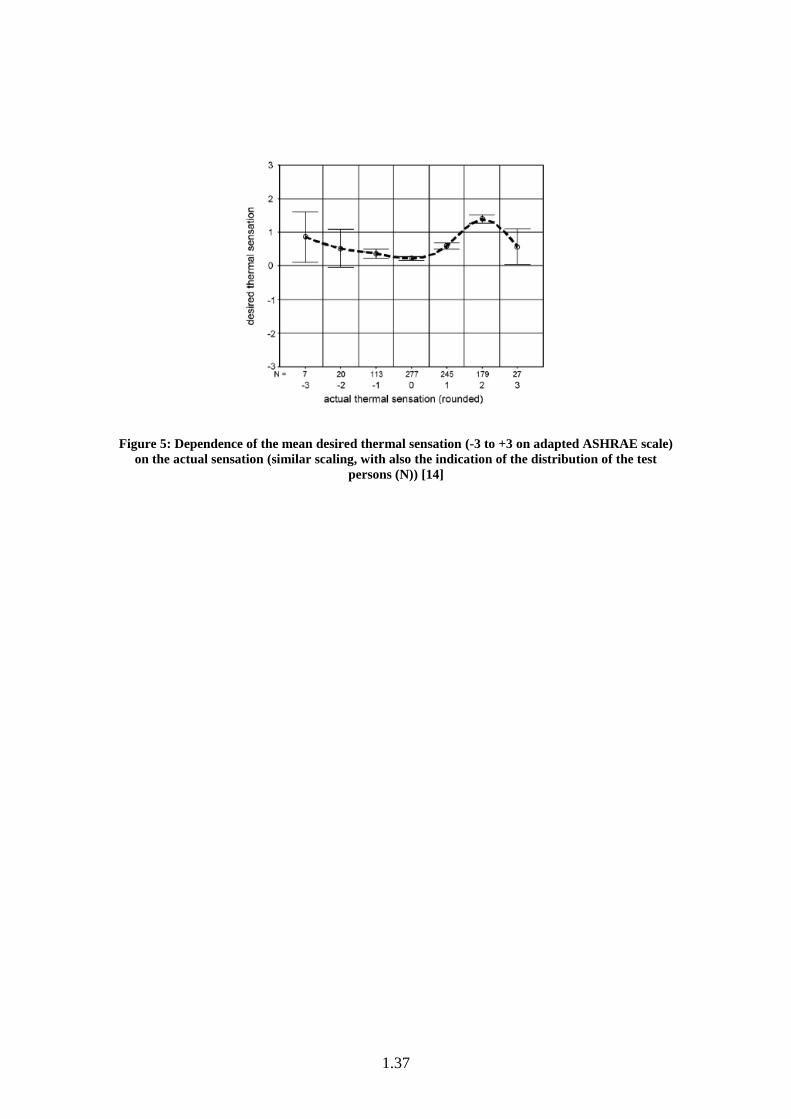
In their enquiries, Humphreys et al., however, found an asymmetric relation between the

desired thermal sensation and the actual sensation [14], as can be seen in Figure 5. The

data were collected at university lectures and in selected dwellings throughout the UK.

1.21

This asymmetry is also confirmed by the analyses of field study data by Fountain et al.

[46]. They concluded that people‟s preferences for non-neutral thermal sensations are

common, that they vary asymmetrically around neutrality and that, in several cases, they

are influenced by season. De Dear et al. consider this idea of outdoor dependent

temperature ranges [21]. However, they observed no statistical significance in the 95%

confidence level, regardless of building type or acceptability level. Seasonal

dependency can thus not be proven and, in this paper, the comfort band around the

neutral temperature is thus considered having a constant width.

To account for both the enhanced sensitivity for cold versus heat and the non seasonal

dependency, the following format for the temperature ranges is suggested here:

(1 )

upper n

lower n

T T w

T T w

(14)

with upperT = upper limit of comfort band (°C)

lowerT = lower limit of comfort band (°C)

w = width of comfort band (°C)

= constant ( 1 )

In the ASHRAE RP 884 study, De Dear and Brager observed that occupants of

residential buildings showed a low sensitivity to indoor temperature changes [22]; the

gradient of their thermal sensation votes with respect to indoor operative temperature

turned out to be 1 vote for every 3°C to 5 °C change in temperature. Values in the same

range are encountered in work of Oseland [44] and of Van der Linden et al. [24]. This, it

1.22

is concluded in present analysis, defines the width of the comfort zone, the value of w

in equation (14); 5°C in case of a 90% acceptability.

Oseland reported a 7°C comfort band width in case of a 80% acceptability.

This so defined width of the comfort band must thus be asymmetrically split around the

neutral temperature. The thermal sensation at the neutral temperature leads to a value of

0 on the adapted 7 points ASHRAE scale (-3 to +3). From Figure 5 it is clear that the

desired sensation in that case is an average 0.2 above neutral. This causes a 70%-30%

split for the temperature band around neutral, resulting in equal to 0.7.

Additionally, some extreme temperatures will cause restrictions. The above stated limit

of 16°C for the bedroom is to be respected. For all other rooms the absolute lower limit

is set to 18°C. This value is often encountered in the literature ([28],[47],[48]). The

upper limits differ depending on the room; while the stringent limit of 26 °C is accepted

for bedrooms in case of no elevated air speed. Bathrooms and rooms with office like

activities can have acceptable indoor temperatures of up to 30 °C in a 90% acceptability

level and almost 31°C for a 80% level [32].

The following restrictions must therefore be added to the statements of equation (14):

- for bedrooms:

min(26 , )upper nT C T w (15)

min max(16 , (1 ) )nT C T w (16)

- for bathrooms and other rooms:

upper nT T w (17)

1.23

max(18 , (1 ))lower nT C T w (18)

4. Conclusions

Most BES programmes currently have the option to evaluate thermal comfort with the

conventional criteria. These evaluation mechanisms have been set up for steady state,

office-like environments. Based on the literature, present analyses shows that, because

of the wide range of possibilities to adapt to the thermal environment, they are not

adequate in case of residential buildings.

Thermal comfort in residential buildings shows a strong dependency on weather data,

more specific on recent outdoor temperatures. Therefore the relations set up in this

paper link the comfort temperatures to a form of outdoor temperature.

It is stated here that a residential building can be split up in three zones with markedly

different thermal comfort requirements; bathroom, bedroom and other rooms. For each

of these zones, the neutral temperatures, defined in present analysis, are based on

measurements described in the literature and in that sense do consider the special case

of each of the zones. The resulting curves for the comfort temperatures, with a

corresponding neutral thermal sensation, show a steeper slope for warmer outdoor

conditions. This is due people adapting more easily to heat than they do to cold.

The asymmetric comfort band around this neutral temperature is set for the same reason.

However, both the neutral temperatures and the comfort bands are restricted by upper

and lower limits. These limits have here been defined based on information of the

World Health Organisation and available experimental data.

1.24

The resulting correlations indoor-outdoor temperature are presented in an algorithmic

way to facilitate implementation in any BES code.

Acknowledgements

The help of Richard de Dear is greatly appreciated. Also the help, advice and

enthusiasm of Jan Hensen, Stanley Kurvers and Arnold Janssens has been encouraging.

References

[1] ESRU, Released version 11.4, http://www.esru.strath.ac.uk/

Programs/ESP-r_CodeDoc/esrures/comfort.F.html, 2007

[2] Welfonder T., Hiller M., Holst S., Knirsch A., Improvements on the capabilities

of TRNSYS, Eight International IBPSA Conference, Eindhoven, The Netherlands,

August 11-14, 2003, pp 1377-1384

[3] Kalyanova O., Heiselberg P., Comparative Validation of Building Simulation

Software: Modeling of Double facades; Final Report, IEA ECBCS Annex 43/SHC Task

34, Validation of Building Energy Simulation tools, Subtask E, 2007, p231

[4] ANSI/ASHRAE 55-2004, Thermal Environmental Conditions for Human

Occupancy, American Society of Heating, Refrigerating and Air-conditioning

Engineers, Inc. Atlanta, USA, 2004

[5] Fanger P., “Thermal Comfort: Analysis and applications in environmental

Engineering”. McGraw-Hill Book Company, United States, 1970

1.25

[6] ISO 7730, Ergonomics of the thermal environment – Analytical determination

and interpretation of thermal comfort using the PMV and PPD indices and local thermal

comfort criteria, International Organisation for standardization, Switserland, 2005

[7] Olesen B., Parsons K., Introduction to thermal comfort standards and to the

proposed new version of EN ISO 7730, Energy and Buildings 2002;34:537-11

[8] Jones B., Capabilities and limitations of thermal models, Smart Controls and

Thermal Comfort Project, Final Report (Confidential), Oxford Brookes University,

2000, p 112-121

[9] Humphreys M., Nicol J., “The validity of ISO-PMV for predicting comfort votes

for every-day thermal environments”. Energy & Buildings, 2002;34: p 667-7

[10] Stoops J., A possible connection between thermal comfort and health, paper

LBNL 55134, Lawrence Berkeley National Laboratory, University of California, 2004

[11] Jokl M., Kabele K., “The substitution of comfort PMV values by a new

experimental operative temperature”. Electronic proceedings of Clima 2007 WellBeing

Indoors, Helsinki, Finland

[12] Brager G., de Dear R., “Thermal adaptation in the built environment: a literature

overview”. Energy & Buildings, 1998;27: p 83-7

[13] Kurvers S., personal communication, 2007

1.26

[14] Humphreys M., Hancock M., “Do people like to feel „neutral‟? Exploring the

variation of the desired thermal sensation on th ASHRAE scale”. Energy & Buildings,

2007;39: p 867-11

[15] Shove E., Social, architectural and environmental convergence, Environmental

Diversity in Architecture, Koen Steemers, Mary Ann Steane (Eds), 2004

[16] Holmes M., Hacker J., “Climate change, thermal comfort and energy: Meeting

the design challenges of the 21st century”. Energy & Buildings, 2007;39: p 802-12

[17] Fiala D., Lomas K., The dynamic effect of adaptive human responses in the

sensation of thermal comfort, Moving Thermal Comfort Standards into the 21st Century,

Windsor, UK, Conference Proceedings, 2001, p 147-157

[18] Baker N., Standeven M., Thermal comfort for free-running buildings, Energy

and Buildings, 1996;23: p 175-7

[19] Hensen J., “Literature review on thermal comfort in transient conditions”.

Building and Environment, 1990;25: p 309-7

[20] Humphreys M., Nicol J., Understanding the adaptive approach to thermal

comfort, ASHRAE technical bulletin, 1998;14: p1-14

[21] de Dear R., Brager G., Developing an adaptive model of thermal comfort and

preference; Final Report Ashrae RP-884, Macquarie Research Ltd., Macquarie

University, Sydney, Australia, 1997

1.27

[22] de Dear R., Brager G., Developing an adaptive model of thermal comfort and

preference, ASHRAE transactions, 1998;104 (1.a): p 145-12

[23] Morgan C., de Dear R., Weather, clothing and thermal adaptation to indoor

climate, Climate Research, 2003;24: p 267-17

[24] van der Linden A., Boerstra A., Raue A., Kurvers S., de Dear R., Adaptiv

etemperature limits: A new guideline in the netherlands. A new approach for the

assessment of building performance with respect to thermal indoor climate, Energy and

Buildings, 2006;38: p 8-9

[25] Nicol F., McCartney K.,“Smart Controls and Thermal comfort Project: Final

Report (Confidential)”, Oxford Brookes University, 2000

[26] McCartney K., Nicol J., Developing an adaptive control algorithm for Europe:

Results of the Scats project, Energy and Buildings, 2002;34:p 623-12

[27] De Dear R., Brager G., “Thermal comfort in naturally ventilated buildings:

revisions to ASHRAE Standard 55”. Energy & Buildings, 2002;34: p 549-12

[28] K. Parsons, 2002, the effect of gender, acclimation state, the opportunity to

adjust clothing and physical disability on requirements for thermal comfort, Energy and

Buildings, vol. 34, pp 593-599

[29] Lammers J., Human factors, energy conservation and design practice, technical

University of Eindhoven, the Netherlands, PhD thesis, 1978

1.28

[30] Tochihara Y., Kimura Y., Yadoguchi I., Nomura M., thermal responses to air

temperature before, during and after bathing, Proceedings of International Conference

of Environmental Ergonomics, San Diego, 1998, USA pp 309-313

[31] Zingano B., A discussion on thermal comfort with reference to bath water

temperature to deduce a midpoint of the thermal comfort zone, Renewable

Energy,2001;23: p 41-6

[32] Kurvers S., van der Lindenn A., Boerstra A., Raue A., Adaptieve

Temperatuurgrenswaarden (ATG), ISSO 74: een nieuwe richtlijn voor de beoordeling van

het thermisch binnenklimaat, Deel 1: Theoretische achtergronden, TvvL Magazine, juni

2005 (In Dutch)

[33] Maeyens J., Janssens A., Breesch H., Ontwerpregels voor zomercomfort in

woningen, Master‟s thesis, 2001, Division of Architecture, Department of applied

sciences, University of Gent, Belgium (In Dutch)

[34] CIBSE, Guide A: Environmental Design, Chartered Institution of Building

Services Engineers, London, 2006

[35] Humphreys M., The influence of season and ambient temperature on human

clothing behaviour In: Indoor Climate Eds.: P. Fanger & O Valbjorn, Danish Building

Research, Copenhagen, 1979

[36] Janssens A., Vandepitte A., Analysis of indoor climate measurements in recently

built Belgian dwelling, IEA annex 41, report n° A41-T3-B-06-10, University of Ghent,

Belgium, departments of Architecture, 2006

1.29

[37] Vandepitte A., Analyse van binneklimaatmetingen in woningen, Masters thesis,

2006, Department of Architecture and Urban Planning, UGent, Belgium (In Dutch)

[38] Chalkey J., Cater H., “Thermal environment”. The Architectural Press LTD,

London, 1968.

[39] Collins K., Low indoor temperatures and morbidity in the elderly, Age and

Ageing,1986;15: p 212-8

[40] Hartley A., West Midlands Public Health Observatory: Health Issues; Fuel

poverty, consulted online via www.wmpho.org.uk, December 2007

[41] Peeters L., van der Veken J., Hens H., Helsen L., D‟haeseleer W., Control of

heating systems in residential buildings; current practice, Energy and Buildings,

2008;40: p 1446-11

[42] Kiekens K., Helsen L., Analyse en simulatie van installaties voor de

gecombineerde productie van sanitair warm water en ruimteverwarming in lage

energiewoningen, Masters thesis, 2007, Applied mechanics and energy conversion,

KULeuven, Belgium (in Dutch)

[43] Oseland N., Predicted and reported thermal sensation in climate chambers,

offices and homes, Energy and Buildings, 1995;23: p 105-10

[44] Oseland N., A comparison of the predicted and reported thermal sensation vote

in homes during winter and summer, Energy and Buildings, 1994;21: p 45-9

1.30

[45] Henze G., Pfafferot J., Herkel S., Felsmann C., “Impact of adaptive comfort

criteria and heat waves on optimal building thermal mass control”. Energy & Buildings,

2007;39: p 221-14

[46] Fountain M., Brager G., de Dear R., “Expectations of indoor climate control”.

Energy & Buildings, 1996;24: p 179-3

[47] Healy J., Clinch P., Fuel poverty, thermal comfort and occupancy: results of a

national household survey in Ireland, Applied Energy, 2002;73:p 329-14

[48] Ubbelohde M., Loisos G., McBride R., “Comfort Reports: Advanced comfort

criteria and adapted comfort & Human comfort studies; section 1: advanced comfort

criteria for ACC house”. Davis Energy Group for the California Energy Commission,

2004

1.31

Figure Captions

Figure 1: Predicted Percentage of Dissatisfied (PPD) as a function of Predicted Mean

Vote (PMV).

Figure 2: Temperature limits as a function of the outdoor temperature Te,ref for different

levels of acceptability. This for the general case of persons dressed according to the

season and performing office-like activities. From [24].

Figure 3: Daily average bedroom temperature in Belgium as function of Te,ref:

minimum, maximum , 95-, 50-, and 5-percentiles [adapted from [37]. The thick lines

indicate curves defined in current work. The black lines indicate the ATL 90-, 80- and

65-accetability limits.

Figure 4: Daily average living room temperature in Belgium as function of Te,ref:

minimum, maximum , 95-, 50-, and 5-percentiles [adapted from [37]. The thick lines

indicate curves defined in current work. The black lines indicate the ATL 90-, 80- and

65-accetability limits.

1.32

Figure 5: Dependence of the mean desired thermal sensation (-3 to +3 on adapted

ASHRAE scale) on the actual sensation (similar scaling, with also the indication of the

distribution of the test persons (N)) [14]

1.33

Figures

Figure 1: Predicted Percentage of Dissatisfied (PPD) as a function of Predicted Mean Vote (PMV).

1.34

Figure 2: Temperature limits as a function of the outdoor temperature Te,ref for different levels of

acceptability. This for the general case of persons dressed according to the season and performing

office-like activities. From [24].

Te,ref (°C)

Ind

oor

op

erat

ive

tem

per

ature

(°C

)

1.35

Figure 3: Daily average bedroom temperature in Belgium as function of Te,ref: minimum, maximum

, 95-, 50-, and 5-percentiles [adapted from [37]. The thick lines indicate curves defined in current

work. The black lines indicate the ATL 90-, 80- and 65-accetability limits.

Dai

ly a

ver

age

bed

roo

m t

emp

erat

ure

(°C

)

Te,ref (°C)

3 4

2

1

1.36

Figure 4: Daily average living room temperature in Belgium as function of Te,ref: minimum,

maximum , 95-, 50-, and 5-percentiles [adapted from [37]. The thick lines indicate curves defined in

current work. The black lines indicate the ATL 90-, 80- and 65-accetability limits.

Dai

ly a

ver

age

bed

roo

m t

emp

erat

ure

(°C

)

Te,ref (°C)

1.37

Figure 5: Dependence of the mean desired thermal sensation (-3 to +3 on adapted ASHRAE scale)

on the actual sensation (similar scaling, with also the indication of the distribution of the test

persons (N)) [14]