Thermal Analysis & Rheology

THERMAL ANALYSIS REVIEWMODULATED DSCTM THEORY

Modulated DSC (MDSC) can be easily understood by comparing it to its well-established precursor, differentialscanning calorimetry (DSC). Conventional DSC is an analytical technique in which the difference in heat flow betweena sample and an inert reference is measured as a function of time and temperature as both the sample and reference aresubjected to a controlled environment of time, temperature, atmosphere and pressure. The schematic of a typical �heatflux� DSC cell is shown in Figure 1. In this design, a metallic disk (made of constantan alloy) is the primary means ofheat transfer to and from the sample and reference. The sample, contained in a metal pan, and the reference (an emptypan) sit on raised platforms formed in the constantan disk. As heat is transferred through the disk, the differential heatflow to the sample and reference is measured by area thermocouples formed by the junction of the constantan disk andchromel wafers which cover the underside of the platforms. Chromel and alumel wires attached to the chromel wafersform thermocouples which directly measure sample temperature. Purge gas is admitted to the sample chamber throughan orifice in the heating block wall midway between the raised platforms. The gas is preheated by circulation throughthe block before entering the sample chamber. The result is a uniform, stable thermal environment which assuresexcellent baseline flatness and exceptional sensitivity (signal-to-noise). In conventional DSC, the temperature regimeseen by the sample and reference is linear heating or cooling at rates from as fast as 200°C/minute to rates as slow as0°C/minute (isothermal).

Figure 1: HEAT FLUX DSC SCHEMATIC

Sample ChamberReference Pan Sample Pan

Gas Purge Inlet

Lid

ChromelDisc

ChromelDisc

HeatingBlock

ThermocoupleJunction

Thermoelectric Disc(Constantan)

Alumel Wire

Chromel WireTA-211B

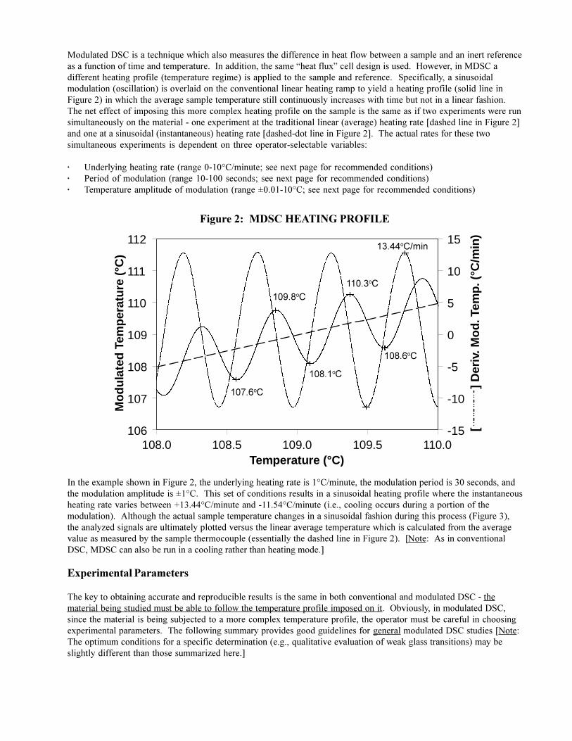
Modulated DSC is a technique which also measures the difference in heat flow between a sample and an inert referenceas a function of time and temperature. In addition, the same �heat flux� cell design is used. However, in MDSC adifferent heating profile (temperature regime) is applied to the sample and reference. Specifically, a sinusoidalmodulation (oscillation) is overlaid on the conventional linear heating ramp to yield a heating profile (solid line inFigure 2) in which the average sample temperature still continuously increases with time but not in a linear fashion.The net effect of imposing this more complex heating profile on the sample is the same as if two experiments were runsimultaneously on the material - one experiment at the traditional linear (average) heating rate [dashed line in Figure 2]and one at a sinusoidal (instantaneous) heating rate [dashed-dot line in Figure 2]. The actual rates for these twosimultaneous experiments is dependent on three operator-selectable variables:

· Underlying heating rate (range 0-10°C/minute; see next page for recommended conditions)· Period of modulation (range 10-100 seconds; see next page for recommended conditions)· Temperature amplitude of modulation (range ±0.01-10°C; see next page for recommended conditions)

Figure 2: MDSC HEATING PROFILE

108.0 108.5 109.0 109.5 110.0106

107

108

109

110

111

112

-15

-10

-5

0

5

10

15

Temperature (°C)

Mod

ulat

ed T

empe

ratu

re (°

C)

[

] D

eriv

. Mod

. Tem

p. (

°C/m

in)13.44oC/min

109.8oC

110.3oC

107.6oC

108.1oC

108.6oC

In the example shown in Figure 2, the underlying heating rate is 1°C/minute, the modulation period is 30 seconds, andthe modulation amplitude is ±1°C. This set of conditions results in a sinusoidal heating profile where the instantaneousheating rate varies between +13.44°C/minute and -11.54°C/minute (i.e., cooling occurs during a portion of themodulation). Although the actual sample temperature changes in a sinusoidal fashion during this process (Figure 3),the analyzed signals are ultimately plotted versus the linear average temperature which is calculated from the averagevalue as measured by the sample thermocouple (essentially the dashed line in Figure 2). [Note: As in conventionalDSC, MDSC can also be run in a cooling rather than heating mode.]

Experimental Parameters

The key to obtaining accurate and reproducible results is the same in both conventional and modulated DSC - thematerial being studied must be able to follow the temperature profile imposed on it. Obviously, in modulated DSC,since the material is being subjected to a more complex temperature profile, the operator must be careful in choosingexperimental parameters. The following summary provides good guidelines for general modulated DSC studies [Note:The optimum conditions for a specific determination (e.g., qualitative evaluation of weak glass transitions) may beslightly different than those summarized here.]

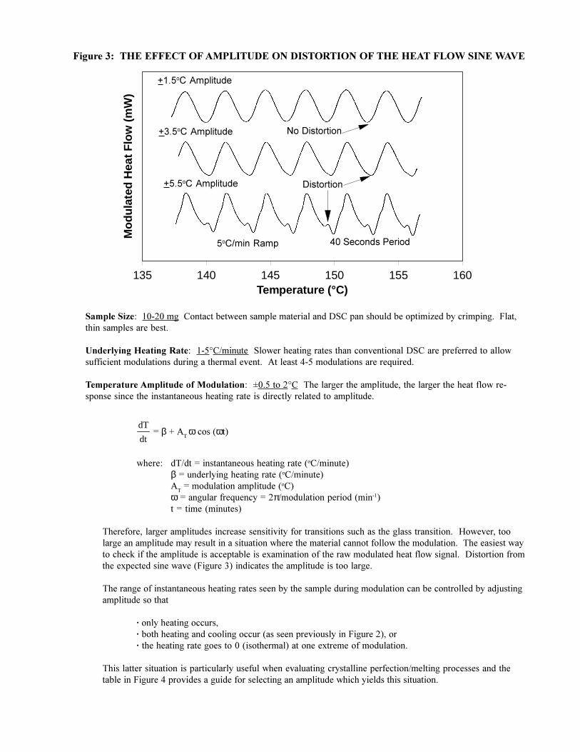
Figure 3: THE EFFECT OF AMPLITUDE ON DISTORTION OF THE HEAT FLOW SINE WAVE

135 140 145 150 155 160Temperature (°C)

Mo

du

late

d H

eat

Flo

w (

mW

)

+1.5oC Amplitude

+3.5oC Amplitude

5oC/min Ramp

No Distortion

Distortion

40 Seconds Period

Sample Size: 10-20 mg Contact between sample material and DSC pan should be optimized by crimping. Flat,thin samples are best.

Underlying Heating Rate: 1-5°C/minute Slower heating rates than conventional DSC are preferred to allowsufficient modulations during a thermal event. At least 4-5 modulations are required.

Temperature Amplitude of Modulation: ±0.5 to 2°C The larger the amplitude, the larger the heat flow re-sponse since the instantaneous heating rate is directly related to amplitude.

dT

dt = β + A

T ω cos (ωt)

where: dT/dt = instantaneous heating rate (oC/minute)β = underlying heating rate (oC/minute)A

T = modulation amplitude (oC)

ω = angular frequency = 2π/modulation period (min-1)t = time (minutes)

Therefore, larger amplitudes increase sensitivity for transitions such as the glass transition. However, toolarge an amplitude may result in a situation where the material cannot follow the modulation. The easiest wayto check if the amplitude is acceptable is examination of the raw modulated heat flow signal. Distortion fromthe expected sine wave (Figure 3) indicates the amplitude is too large.

The range of instantaneous heating rates seen by the sample during modulation can be controlled by adjustingamplitude so that

· only heating occurs,· both heating and cooling occur (as seen previously in Figure 2), or· the heating rate goes to 0 (isothermal) at one extreme of modulation.

This latter situation is particularly useful when evaluating crystalline perfection/melting processes and thetable in Figure 4 provides a guide for selecting an amplitude which yields this situation.

+5.5oC Amplitude

-200 -100 0 100 200 300 400 500

0.10

0.30

1.00

3.00

10.00

Temperature (°C)

Am

plitu

de (

+/-°

C)

0.05

0.07

0.20

0.50

0.70

2.00

5.00

7.00

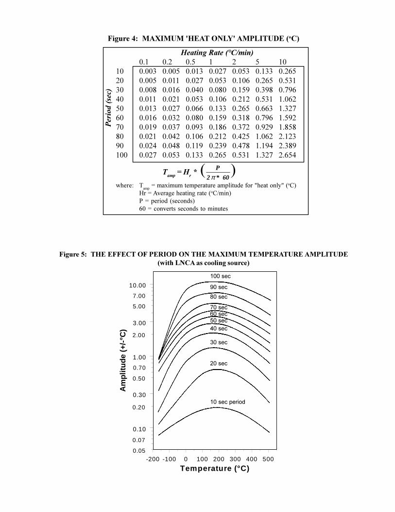
Figure 4: MAXIMUM 'HEAT ONLY' AMPLITUDE (oC)

Heating Rate (°C/min)0.1 0.2 0.5 1 2 5 10

10 0.003 0.005 0.013 0.027 0.053 0.133 0.26520 0.005 0.011 0.027 0.053 0.106 0.265 0.53130 0.008 0.016 0.040 0.080 0.159 0.398 0.79640 0.011 0.021 0.053 0.106 0.212 0.531 1.06250 0.013 0.027 0.066 0.133 0.265 0.663 1.32760 0.016 0.032 0.080 0.159 0.318 0.796 1.59270 0.019 0.037 0.093 0.186 0.372 0.929 1.85880 0.021 0.042 0.106 0.212 0.425 1.062 2.12390 0.024 0.048 0.119 0.239 0.478 1.194 2.389100 0.027 0.053 0.133 0.265 0.531 1.327 2.654

Tamp

= Hr * ( P

2π * 60)

where: Tamp

= maximum temperature amplitude for "heat only" (oC)Hr = Average heating rate (oC/min)P = period (seconds)60 = converts seconds to minutes

Per

iod

(sec

)

100 sec

90 sec

80 sec

70 sec60 sec50 sec40 sec

30 sec

20 sec

10 sec period

Figure 5: THE EFFECT OF PERIOD ON THE MAXIMUM TEMPERATURE AMPLITUDE(with LNCA as cooling source)

Period of Modulation: 40-100 seconds The period and amplitude of modulation are interrelated terms.Figure 5 shows the range of acceptable amplitudes for a given period (with an LNCA as the cooling source).Obviously as the period of modulation increases, the material has longer to respond and the range of accept-able amplitudes increases. Note, however, that smaller amplitudes are still preferred even with longer periodsfor covering a reasonable temperaure range.

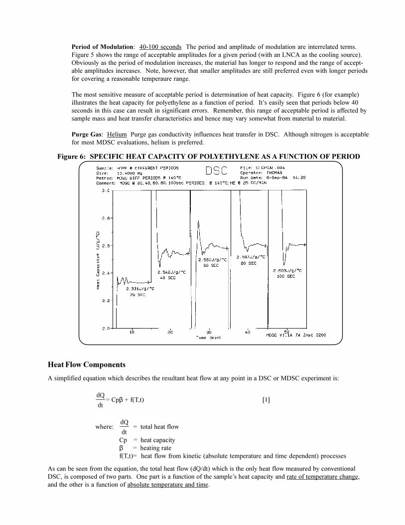
The most sensitive measure of acceptable period is determination of heat capacity. Figure 6 (for example)illustrates the heat capacity for polyethylene as a function of period. It�s easily seen that periods below 40seconds in this case can result in significant errors. Remember, this range of acceptable period is affected bysample mass and heat transfer characteristics and hence may vary somewhat from material to material.

Purge Gas: Helium Purge gas conductivity influences heat transfer in DSC. Although nitrogen is acceptablefor most MDSC evaluations, helium is preferred.

Heat Flow Components

A simplified equation which describes the resultant heat flow at any point in a DSC or MDSC experiment is:

dQ

dt= Cpβ + f(T,t) [1]

where:dQ

dt = total heat flow

Cp = heat capacityβ = heating ratef(T,t)= heat flow from kinetic (absolute temperature and time dependent) processes

As can be seen from the equation, the total heat flow (dQ/dt) which is the only heat flow measured by conventionalDSC, is composed of two parts. One part is a function of the sample�s heat capacity and rate of temperature change,and the other is a function of absolute temperature and time.

Figure 6: SPECIFIC HEAT CAPACITY OF POLYETHYLENE AS A FUNCTION OF PERIOD

Modulated DSC determines the total, as well as these two individual heat flow components, to provide increasedunderstanding of complex transitions in materials. MDSC is able to do this because it effectively uses two heatingrates - the average heating rate which provides total heat flow information and a sinusoidal heating rate which providesheat capacity information from the heat flow that responds to the rate of temperature change.

The individual heat flow components are often referred to by different names as listed below. In the remainder of thispaper they will be called �heat capacity component� (Cpβ) and �kinetic component� (f(T,t)).

Heat Capacity Component Kinetic ComponentReversing heat flow Nonreversing heat flowIn-phase component Out-of-phase componentHeating rate-related component Time dependent component

MDSC Heat Flow Signals

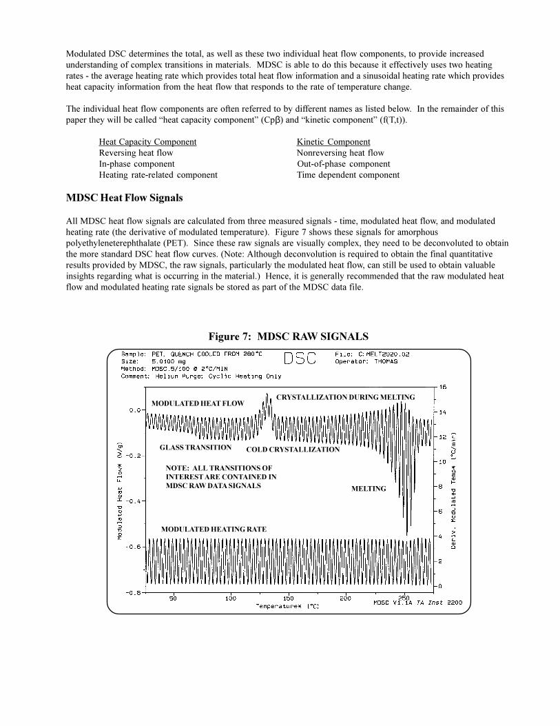
All MDSC heat flow signals are calculated from three measured signals - time, modulated heat flow, and modulatedheating rate (the derivative of modulated temperature). Figure 7 shows these signals for amorphouspolyethyleneterephthalate (PET). Since these raw signals are visually complex, they need to be deconvoluted to obtainthe more standard DSC heat flow curves. (Note: Although deconvolution is required to obtain the final quantitativeresults provided by MDSC, the raw signals, particularly the modulated heat flow, can still be used to obtain valuableinsights regarding what is occurring in the material.) Hence, it is generally recommended that the raw modulated heatflow and modulated heating rate signals be stored as part of the MDSC data file.

Figure 7: MDSC RAW SIGNALS

MODULATED HEAT FLOWCRYSTALLIZATION DURING MELTING

GLASS TRANSITION COLD CRYSTALLIZATION

NOTE: ALL TRANSITIONS OFINTEREST ARE CONTAINED INMDSC RAW DATA SIGNALS MELTING

MODULATED HEATING RATE

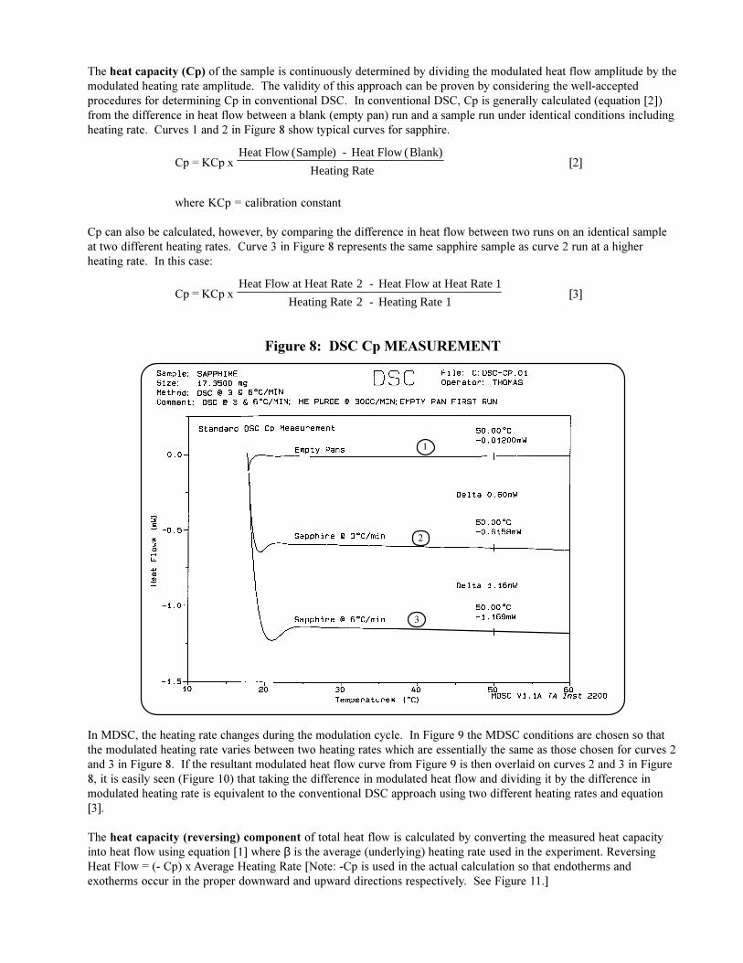
The heat capacity (Cp) of the sample is continuously determined by dividing the modulated heat flow amplitude by themodulated heating rate amplitude. The validity of this approach can be proven by considering the well-acceptedprocedures for determining Cp in conventional DSC. In conventional DSC, Cp is generally calculated (equation [2])from the difference in heat flow between a blank (empty pan) run and a sample run under identical conditions includingheating rate. Curves 1 and 2 in Figure 8 show typical curves for sapphire.

Cp = KCp x Heat Flow (Sample) - Heat Flow (Blank)

Heating Rate[2]

where KCp = calibration constant

Cp can also be calculated, however, by comparing the difference in heat flow between two runs on an identical sampleat two different heating rates. Curve 3 in Figure 8 represents the same sapphire sample as curve 2 run at a higherheating rate. In this case:

Cp = KCp x Heat Flow at Heat Rate 2 - Heat Flow at Heat Rate 1

Heating Rate 2 - Heating Rate 1[3]

Figure 8: DSC Cp MEASUREMENT

1

2

In MDSC, the heating rate changes during the modulation cycle. In Figure 9 the MDSC conditions are chosen so thatthe modulated heating rate varies between two heating rates which are essentially the same as those chosen for curves 2and 3 in Figure 8. If the resultant modulated heat flow curve from Figure 9 is then overlaid on curves 2 and 3 in Figure8, it is easily seen (Figure 10) that taking the difference in modulated heat flow and dividing it by the difference inmodulated heating rate is equivalent to the conventional DSC approach using two different heating rates and equation[3].

The heat capacity (reversing) component of total heat flow is calculated by converting the measured heat capacityinto heat flow using equation [1] where β is the average (underlying) heating rate used in the experiment. ReversingHeat Flow = (- Cp) x Average Heating Rate [Note: -Cp is used in the actual calculation so that endotherms andexotherms occur in the proper downward and upward directions respectively. See Figure 11.]

3

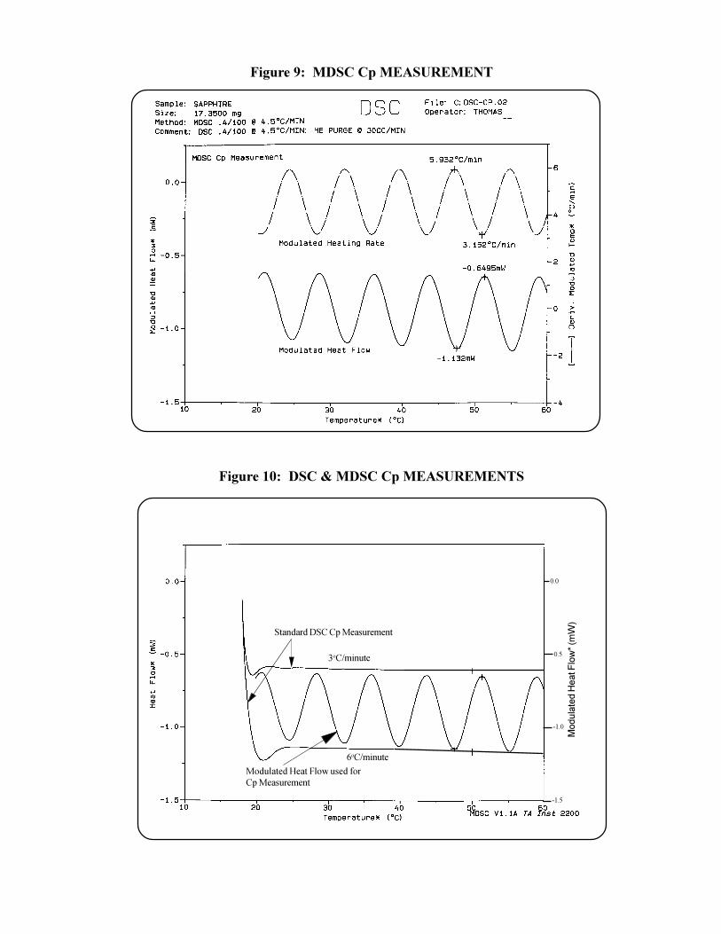
Figure 9: MDSC Cp MEASUREMENT

Figure 10: DSC & MDSC Cp MEASUREMENTS

0.0

0.5

-1.0

-1.5

Standard DSC Cp Measurement

Modulated Heat Flow used forCp Measurement

Mod

ulat

ed H

eat F

low

* (m

W)

3oC/minute

6oC/minute

Figure 11: REVERSING HEAT FLOW FROM MDSC RAW SIGNALS

Figure 12: TOTAL HEAT FLOW FROM MDSC RAW SIGNALS

HEAT CAPACITY

REVERSING HEAT FLOW

TOTAL HEAT FLOW IS CALCULATEDAS THE AVERAGE VALUE OF THEMODULATED HEAT FLOW SIGNAL

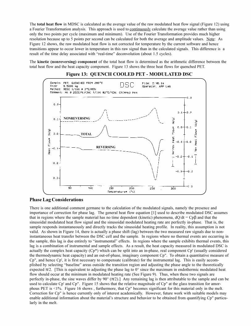
The total heat flow in MDSC is calculated as the average value of the raw modulated heat flow signal (Figure 12) usinga Fourier Transformation analysis. This approach is used to continuously calculate the average value rather than usingonly the two points per cycle (maximum and minimum). Use of the Fourier Transformation provides much higherresolution because up to 5 points per second can be calculated for both the average and amplitude values. Note: AsFigure 12 shows, the raw modulated heat flow is not corrected for temperature by the current software and hencetransitions appear to occur lower in temperature in this raw signal than in the calculated signals. This difference is aresult of the time delay associated with �real-time� deconvolution (about 1.5 cycles).

The kinetic (nonreversing) component of the total heat flow is determined as the arithmetic difference between thetotal heat flow and the heat capacity component. Figure 13 shows the three heat flows for quenched PET.

Figure 13: QUENCH COOLED PET - MODULATED DSC

NONREVERSING

TOTAL

REVERSING

Phase Lag Considerations

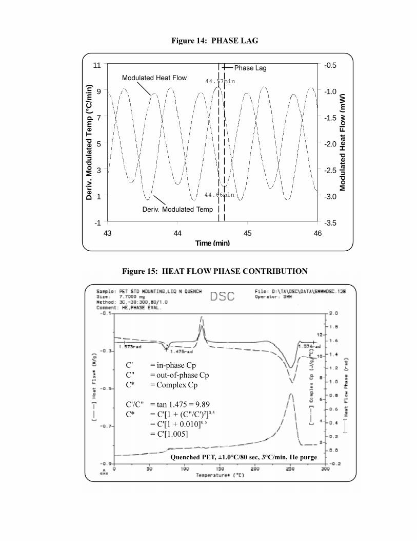
There is one additional comment germane to the calculation of the modulated signals, namely the presence andimportance of correction for phase lag. The general heat flow equation [1] used to describe modulated DSC assumesthat in regions where the sample material has no time dependent (kinetic) phenomena, dQ/dt = Cpβ and that thesinusoidal modulated heat flow signal and the sinusoidal modulated heating rate are perfectly in-phase. That is, thesample responds instantaneously and directly tracks the sinusoidal heating profile. In reality, this assumption is notvalid. As shown in Figure 14, there is actually a phase shift (lag) between the two measured raw signals due to non-instantaneous heat transfer between the DSC cell and the sample. In regions where no thermal events are occurring inthe sample, this lag is due entirely to �instrumental� effects. In regions where the sample exhibits thermal events, thislag is a combination of instrumental and sample effects. As a result, the heat capacity measured in modulated DSC isactually the complex heat capacity (Cp*) which can be split into an in-phase, real component Cp' (usually consideredthe thermodynamic heat capacity) and an out-of-phase, imaginary component Cp". To obtain a quantitative measure ofCp", and hence Cp', it is first necessary to compensate (calibrate) for the instrumental lag. This is easily accom-plished by selecting �baseline� areas outside the transition region and adjusting the phase angle to the theoreticallyexpected π/2. [This is equivalent to adjusting the phase lag to 0° since the maximum in endothermic modulated heatflow should occur at the minimum in modulated heating rate (See Figure 9). Thus, when these two signals areperfectly in-phase, the sine waves differ by 90° (π/2).] Any remaining lag is then attributable to the sample and can beused to calculate Cp' and Cp". Figure 15 shows that the relative magnitude of Cp" at the glass transition for amor-phous PET is <1%. Figure 16 shows , furthermore, that Cp" becomes significant for this material only in the melt.Correction for Cp" is hence currently only of interest academically. However, future work with suitable models mayenable additional information about the material�s structure and behavior to be obtained from quantifying Cp" particu-larly in the melt.

43 44 45 46-1

1

3

5

7

9

11

-3.5

-3.0

-2.5

-2.0

-1.5

-1.0

-0.5

Time (min)

Der

iv. M

odul

ated

Tem

p (°

C/m

in)

Mod

ulat

edH

eatF

low

(mW

)

Figure 14: PHASE LAG

Figure 15: HEAT FLOW PHASE CONTRIBUTION

Quenched PET, ±1.0°C/80 sec, 3°C/min, He purge

C' = in-phase CpC" = out-of-phase CpC* = Complex Cp

C'/C" = tan 1.475 = 9.89C* = C'[1 + (C"/C')2]0.5

= C'[1 + 0.010]0.5

= C'[1.005] [

]

Phase Lag

44.57min

Deriv. Modulated Temp

44.66min

Modulated Heat Flow

Figure 16: PHASE-CORRECTED HEAT FLOW SIGNALSQUENCHED PET

TA-211B

-3

-2.5

-2

-1.5

-1

-0.5

0

0.5

1

1.5

2

0 25 50 75 100 125 150 175 200 225 250 275

Temperature (°C)

Hea

t F

low

(m

W)

Reversing Heat Flow

Nonreversing Heat Flow

CorrectedData

Temperature (oC)

TA Instruments S.A.R.L.Paris, FranceTelephone: 33-01-30489460Fax: 33-01-30489451

TA Instruments, Inc.109 Lukens DriveNew Castle, DE 19720Telephone: (302) 427-4000Fax: (302) 427-4001

For more information or to place an order, contact:

TA Instruments, Ltd.Leatherhead, EnglandTelephone: 44-1-372-360363Fax: 44-1-372-360135

TA Instruments N.V./S.A.Gent, BelgiumTelephone: 32-9-220-79-89Fax: 32-9-220-83-21

TA Instruments GmbHAlzenau, GermanyTelephone: 49-6023-30044Fax: 49-6023-30823

TA Instruments Japan K.K.Tokyo, JapanTelephone: 813-3450-0981Fax: 813-3450-1322

Internet: http://www.tainst.com

Thermal Analysis & RheologyA SUBSIDIARY OF WATERS CORPORATION