theory of hplc quantitative and qualitative hplc

Quantitative & Qualitative HPLC

i Wherever you see this symbol, it is important to access the on-line course as there

is interactive material that cannot be fully shown in this reference manual.

1

© www.chromacademy.com

Contents Page

1 Aims and Objectives 2 2 Qualitative Analysis Overview 3 3 Peak Identification and Assignment 4 4 Sample Spiking 5 5 Spectral Peak Identification 6-8

5.1. Peak Purity 7 5.2. Spectral Characterization 8

6 Quantitative Analysis Overview 9 7 Chromatographic Requirements 10 8 Peak Integration Events 11-12

8.1. Integration Events 12 9 Peak Height or Peak Area 13 10 Principles of Quantitative Analysis 14 11 Area%/Height% (Normalization) 15 12 External Standard Quantitation 16-17 13 Calibration Curve 18-20

13.1. Statistical Information 19-20 14 External Standard Multi-Level Calibration 21-24

14.1. Calibration Curve Information 23-24 15 External Standard Multi-Level Calibration Curve - Typical Calculation 25-26 16 Internal Standard Analysis 27-29 17 Multi-Level Calibration Curve 30-31

2


1. Aims and Objectives

Aims

To define Quantitative HPLC and explain the information that can be derived from this type of HPLC analysis

To examine the use of Peak Height or Area in quantitative calculations and to investigate Integration of chromatographic peaks

To explain the use of Calibration and Calibration curves in Quantitative HPLC

To outline the principles of Single and Multi-level calibration in Quantitative analysis

To investigate practical uses of External Standard, Internal Standard and Normalization methods of Quantitative analysis

To outline example calculations for the various Quantitative methods

Objectives

At the end of this Section you should be able to:

To define Qualitative HPLC and explain the information that can be derived from this type of HPLC analysis

To define and explain the principles of peak identification and analyte characterization from a practical perspective

3


2. Qualitative Analysis Overview

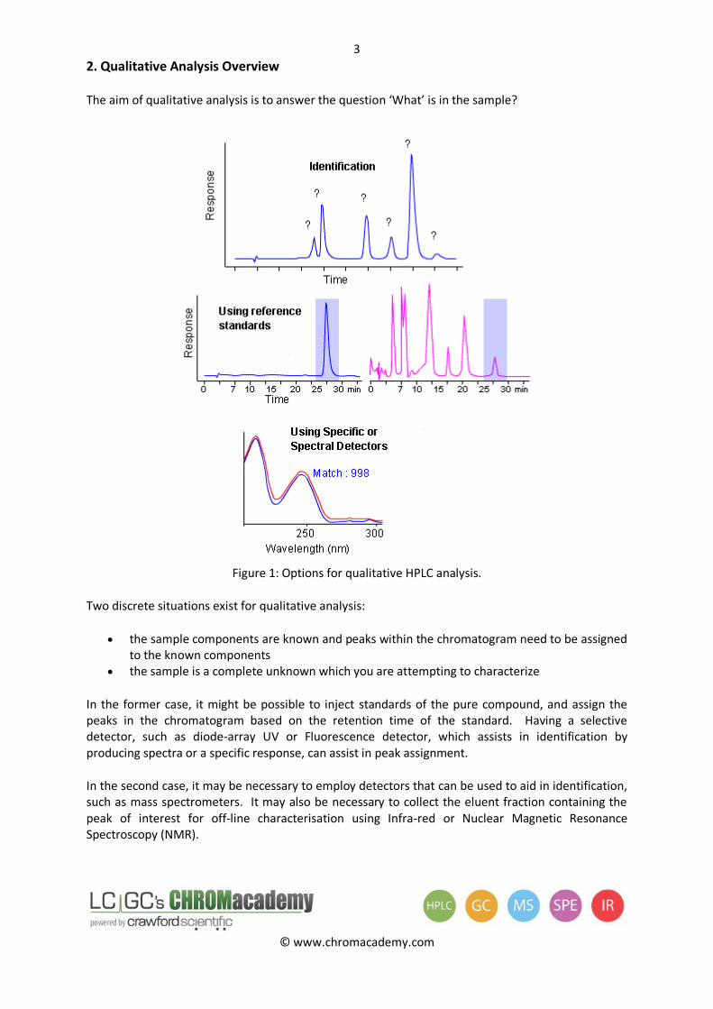
The aim of qualitative analysis is to answer the question ‘What’ is in the sample?

Figure 1: Options for qualitative HPLC analysis.

Two discrete situations exist for qualitative analysis:

the sample components are known and peaks within the chromatogram need to be assigned to the known components

the sample is a complete unknown which you are attempting to characterize

In the former case, it might be possible to inject standards of the pure compound, and assign the peaks in the chromatogram based on the retention time of the standard. Having a selective detector, such as diode-array UV or Fluorescence detector, which assists in identification by producing spectra or a specific response, can assist in peak assignment.

In the second case, it may be necessary to employ detectors that can be used to aid in identification, such as mass spectrometers. It may also be necessary to collect the eluent fraction containing the peak of interest for off-line characterisation using Infra-red or Nuclear Magnetic Resonance Spectroscopy (NMR).

4


3. Peak Identification and Assignment

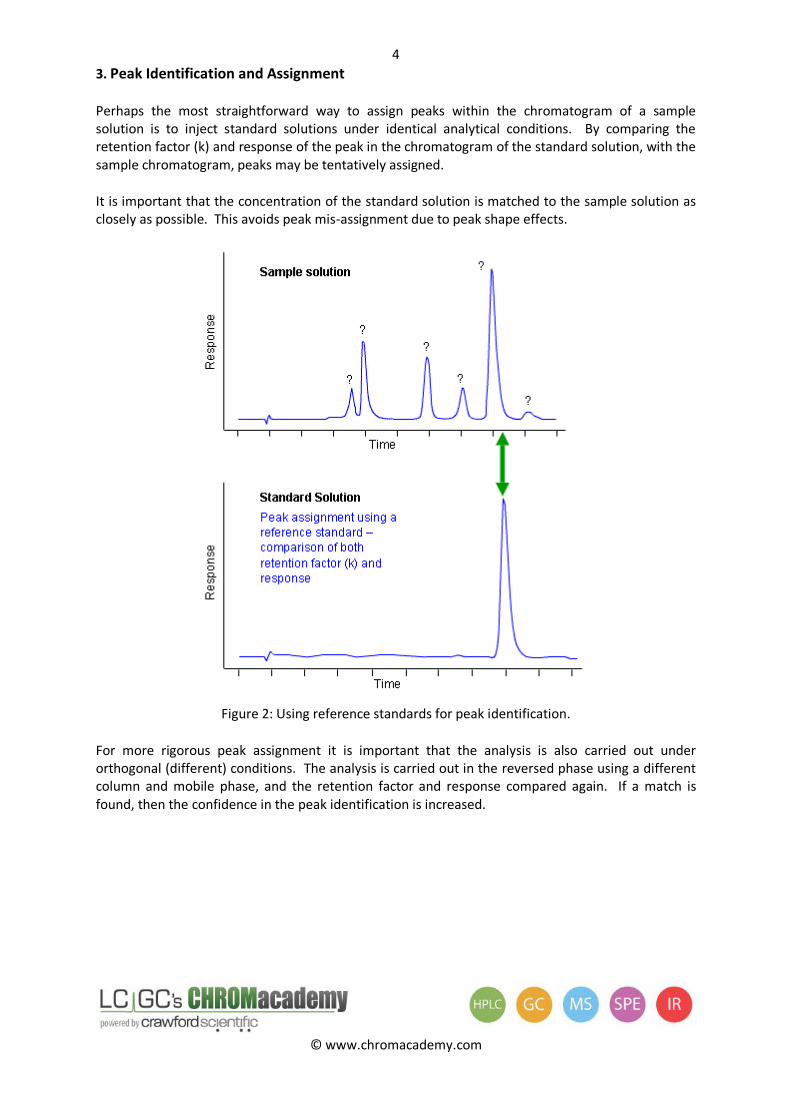
Perhaps the most straightforward way to assign peaks within the chromatogram of a sample solution is to inject standard solutions under identical analytical conditions. By comparing the retention factor (k) and response of the peak in the chromatogram of the standard solution, with the sample chromatogram, peaks may be tentatively assigned.

It is important that the concentration of the standard solution is matched to the sample solution as closely as possible. This avoids peak mis-assignment due to peak shape effects.

Figure 2: Using reference standards for peak identification.

For more rigorous peak assignment it is important that the analysis is also carried out under orthogonal (different) conditions. The analysis is carried out in the reversed phase using a different column and mobile phase, and the retention factor and response compared again. If a match is found, then the confidence in the peak identification is increased.

5


4. Sample Spiking

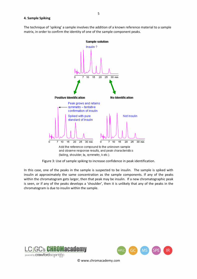
The technique of ‘spiking’ a sample involves the addition of a known reference material to a sample matrix, in order to confirm the identity of one of the sample component peaks.

Figure 3: Use of sample spiking to increase confidence in peak identification.

In this case, one of the peaks in the sample is suspected to be insulin. The sample is spiked with insulin at approximately the same concentration as the sample components. If any of the peaks within the chromatogram gets larger, then that peak may be insulin. If a new chromatographic peak is seen, or if any of the peaks develops a ‘shoulder’, then it is unlikely that any of the peaks in the chromatogram is due to insulin within the sample.

6


5. Spectral Peak Identification

The identification and assignment of peaks within sample chromatograms using retention time alone can be unreliable.

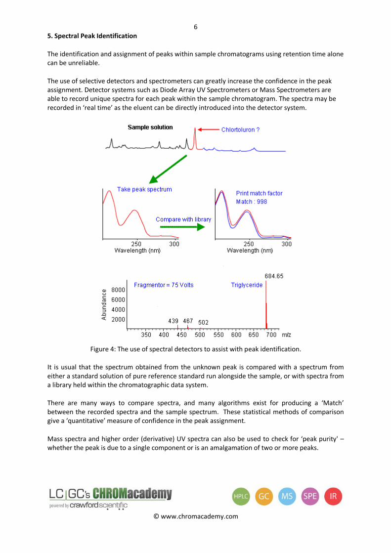
The use of selective detectors and spectrometers can greatly increase the confidence in the peak assignment. Detector systems such as Diode Array UV Spectrometers or Mass Spectrometers are able to record unique spectra for each peak within the sample chromatogram. The spectra may be recorded in ‘real time’ as the eluent can be directly introduced into the detector system.

Figure 4: The use of spectral detectors to assist with peak identification.

It is usual that the spectrum obtained from the unknown peak is compared with a spectrum from either a standard solution of pure reference standard run alongside the sample, or with spectra from a library held within the chromatographic data system.

There are many ways to compare spectra, and many algorithms exist for producing a ‘Match’ between the recorded spectra and the sample spectrum. These statistical methods of comparison give a ‘quantitative’ measure of confidence in the peak assignment.

Mass spectra and higher order (derivative) UV spectra can also be used to check for ‘peak purity' – whether the peak is due to a single component or is an amalgamation of two or more peaks.

7


5.1. Peak Purity

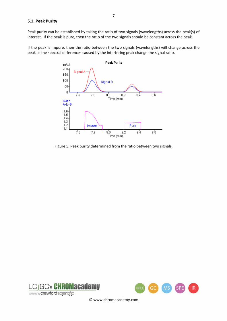
Peak purity can be established by taking the ratio of two signals (wavelengths) across the peak(s) of interest. If the peak is pure, then the ratio of the two signals should be constant across the peak.

If the peak is impure, then the ratio between the two signals (wavelengths) will change across the peak as the spectral differences caused by the interfering peak change the signal ratio.

Figure 5: Peak purity determined from the ratio between two signals.

8


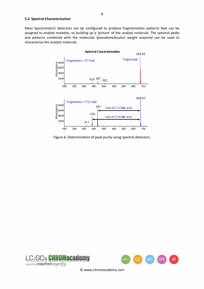
5.2. Spectral Characterization

Mass Spectrometric detectors can be configured to produce fragmentation patterns that can be assigned to analyte moieties, so building up a ‘picture’ of the analyte molecule. The spectral peaks and patterns combined with the molecular (pseudomolecular) weight acquired can be used to characterise the analyte molecule.

Figure 6: Determination of peak purity using spectral detectors.

9


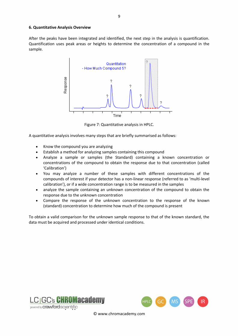
6. Quantitative Analysis Overview

After the peaks have been integrated and identified, the next step in the analysis is quantification. Quantification uses peak areas or heights to determine the concentration of a compound in the sample.

Figure 7: Quantitative analysis in HPLC.

A quantitative analysis involves many steps that are briefly summarised as follows:

Know the compound you are analyzing Establish a method for analyzing samples containing this compound Analyze a sample or samples (the Standard) containing a known concentration or

concentrations of the compound to obtain the response due to that concentration (called ‘Calibration’)

You may analyze a number of these samples with different concentrations of the compounds of interest if your detector has a non-linear response (referred to as ‘multi-level calibration’), or if a wide concentration range is to be measured in the samples

analyze the sample containing an unknown concentration of the compound to obtain the response due to the unknown concentration

Compare the response of the unknown concentration to the response of the known (standard) concentration to determine how much of the compound is present

To obtain a valid comparison for the unknown sample response to that of the known standard, the data must be acquired and processed under identical conditions.

10


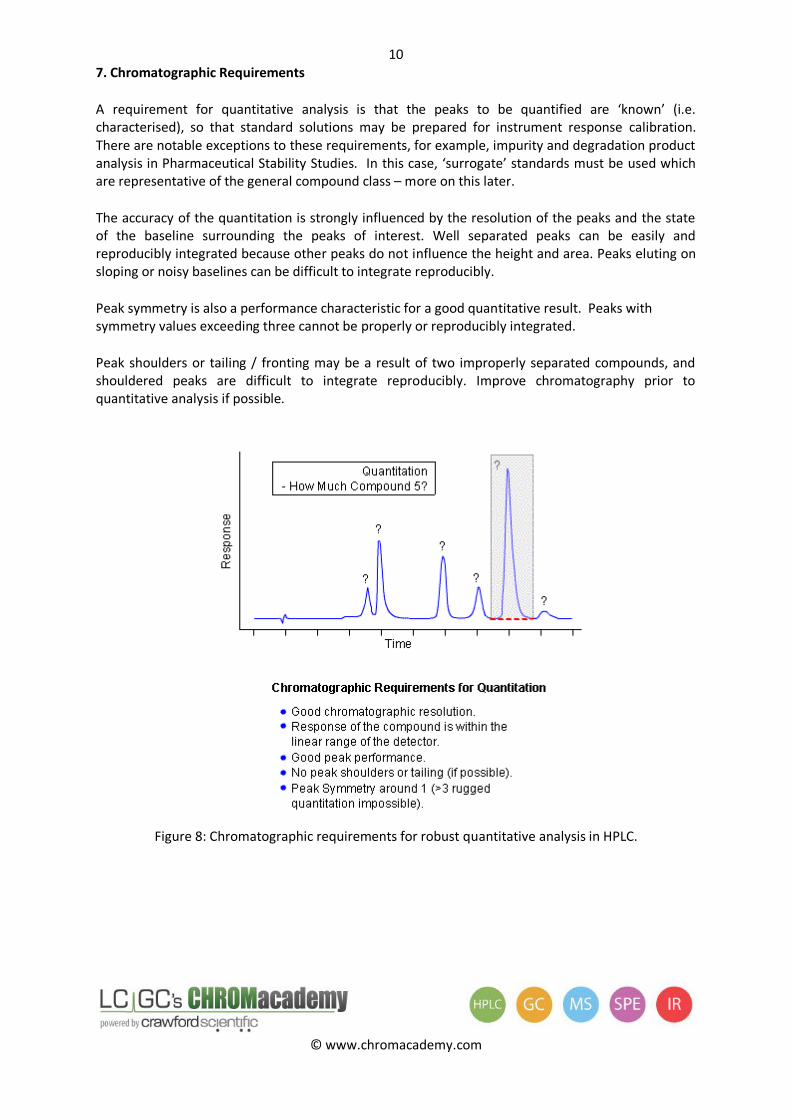
7. Chromatographic Requirements

A requirement for quantitative analysis is that the peaks to be quantified are ‘known’ (i.e. characterised), so that standard solutions may be prepared for instrument response calibration. There are notable exceptions to these requirements, for example, impurity and degradation product analysis in Pharmaceutical Stability Studies. In this case, ‘surrogate’ standards must be used which are representative of the general compound class – more on this later.

The accuracy of the quantitation is strongly influenced by the resolution of the peaks and the state of the baseline surrounding the peaks of interest. Well separated peaks can be easily and reproducibly integrated because other peaks do not influence the height and area. Peaks eluting on sloping or noisy baselines can be difficult to integrate reproducibly.

Peak symmetry is also a performance characteristic for a good quantitative result. Peaks with symmetry values exceeding three cannot be properly or reproducibly integrated.

Peak shoulders or tailing / fronting may be a result of two improperly separated compounds, and shouldered peaks are difficult to integrate reproducibly. Improve chromatography prior to quantitative analysis if possible.

Figure 8: Chromatographic requirements for robust quantitative analysis in HPLC.

11


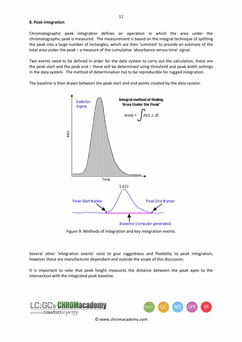
8. Peak Integration

Chromatographic peak integration defines an operation in which the area under the chromatographic peak is measured. The measurement is based on the integral technique of splitting the peak into a large number of rectangles, which are then ‘summed’ to provide an estimate of the total area under the peak – a measure of the cumulative ‘absorbance versus time’ signal.

Two events need to be defined in order for the data system to carry out the calculation, these are the peak start and the peak end – these will be determined using threshold and peak width settings in the data system. The method of determination has to be reproducible for rugged integration.

The baseline is then drawn between the peak start and end points created by the data system.

Figure 9: Methods of integration and key integration events.

Several other ‘integration events’ exist to give ruggedness and flexibility to peak integration, however these are manufacturer dependant and outside the scope of this discussion.

It is important to note that peak height measures the distance between the peak apex to the intersection with the integrated peak baseline.

12


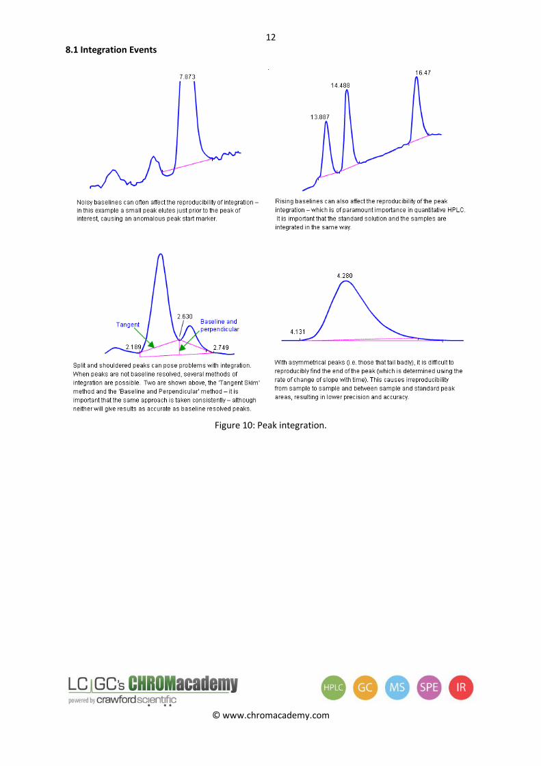
8.1 Integration Events

Figure 10: Peak integration.

13


9. Peak Height or Peak Area

For most HPLC analyses, peak areas are used for quantitative calculations, although, in most cases, equivalent results may be achieved with peak height.

Peak area is especially useful because HPLC peaks may be tailed. In this case, because peak heights may vary (although area will remain constant), area vales are more repeatable.

There are however, instances when peak height calculations may be better. For trace analysis, when the peak of interest is very small, use peak height for calculations, this reduces the error sustained in small changes in peak start and end time variation.

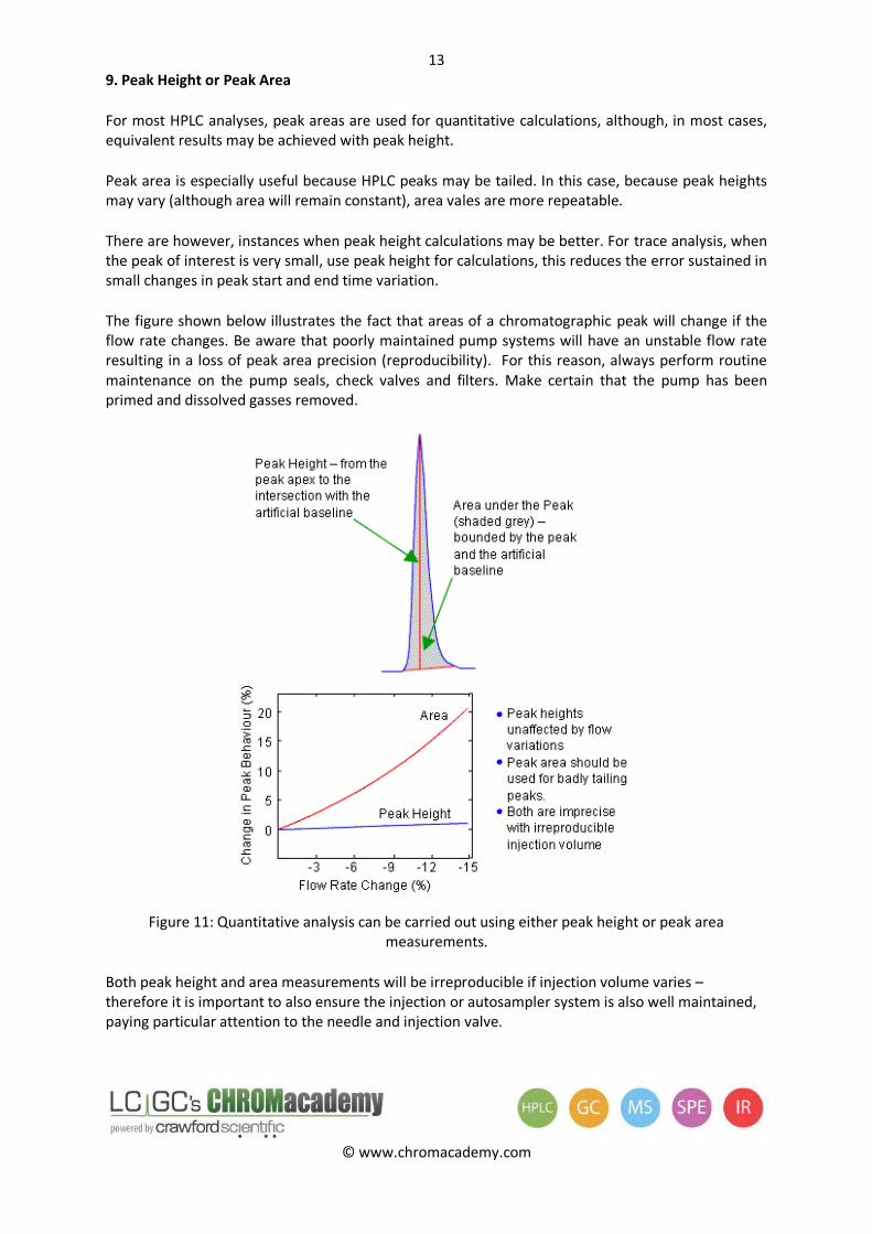
The figure shown below illustrates the fact that areas of a chromatographic peak will change if the flow rate changes. Be aware that poorly maintained pump systems will have an unstable flow rate resulting in a loss of peak area precision (reproducibility). For this reason, always perform routine maintenance on the pump seals, check valves and filters. Make certain that the pump has been primed and dissolved gasses removed.

Figure 11: Quantitative analysis can be carried out using either peak height or peak area

measurements.

Both peak height and area measurements will be irreproducible if injection volume varies – therefore it is important to also ensure the injection or autosampler system is also well maintained, paying particular attention to the needle and injection valve.

14


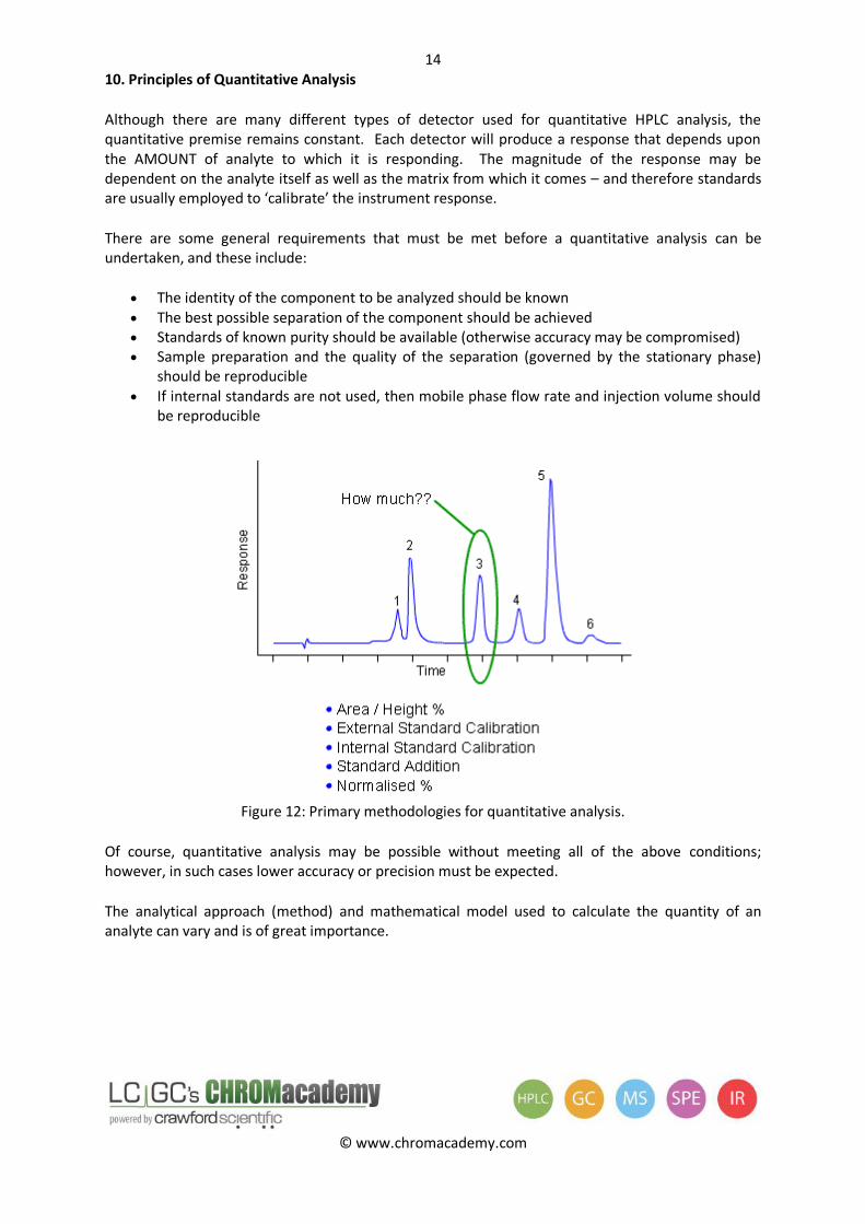
10. Principles of Quantitative Analysis

Although there are many different types of detector used for quantitative HPLC analysis, the quantitative premise remains constant. Each detector will produce a response that depends upon the AMOUNT of analyte to which it is responding. The magnitude of the response may be dependent on the analyte itself as well as the matrix from which it comes – and therefore standards are usually employed to ‘calibrate’ the instrument response.

There are some general requirements that must be met before a quantitative analysis can be undertaken, and these include:

The identity of the component to be analyzed should be known The best possible separation of the component should be achieved Standards of known purity should be available (otherwise accuracy may be compromised) Sample preparation and the quality of the separation (governed by the stationary phase)

should be reproducible If internal standards are not used, then mobile phase flow rate and injection volume should

be reproducible

Figure 12: Primary methodologies for quantitative analysis.

Of course, quantitative analysis may be possible without meeting all of the above conditions; however, in such cases lower accuracy or precision must be expected.

The analytical approach (method) and mathematical model used to calculate the quantity of an analyte can vary and is of great importance.

15


11. Area %/ Height % (Normalization)

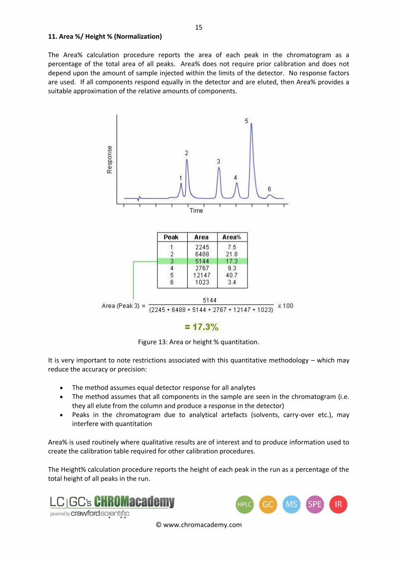
The Area% calculation procedure reports the area of each peak in the chromatogram as a percentage of the total area of all peaks. Area% does not require prior calibration and does not depend upon the amount of sample injected within the limits of the detector. No response factors are used. If all components respond equally in the detector and are eluted, then Area% provides a suitable approximation of the relative amounts of components.

Figure 13: Area or height % quantitation.

It is very important to note restrictions associated with this quantitative methodology – which may reduce the accuracy or precision:

The method assumes equal detector response for all analytes The method assumes that all components in the sample are seen in the chromatogram (i.e.

they all elute from the column and produce a response in the detector) Peaks in the chromatogram due to analytical artefacts (solvents, carry-over etc.), may

interfere with quantitation

Area% is used routinely where qualitative results are of interest and to produce information used to create the calibration table required for other calibration procedures.

The Height% calculation procedure reports the height of each peak in the run as a percentage of the total height of all peaks in the run.

16


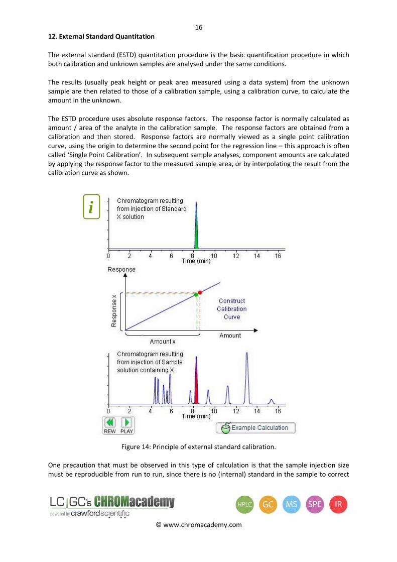
12. External Standard Quantitation

The external standard (ESTD) quantitation procedure is the basic quantification procedure in which both calibration and unknown samples are analysed under the same conditions.

The results (usually peak height or peak area measured using a data system) from the unknown sample are then related to those of a calibration sample, using a calibration curve, to calculate the amount in the unknown.

The ESTD procedure uses absolute response factors. The response factor is normally calculated as amount / area of the analyte in the calibration sample. The response factors are obtained from a calibration and then stored. Response factors are normally viewed as a single point calibration curve, using the origin to determine the second point for the regression line – this approach is often called ‘Single Point Calibration’. In subsequent sample analyses, component amounts are calculated by applying the response factor to the measured sample area, or by interpolating the result from the calibration curve as shown.

Figure 14: Principle of external standard calibration.

One precaution that must be observed in this type of calculation is that the sample injection size must be reproducible from run to run, since there is no (internal) standard in the sample to correct

i

17


for variations in injection size or sample preparation. The method type also assumes a linear detector response and that samples do not contain a wide range of analyte concentrations.

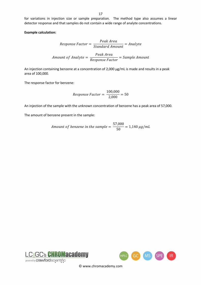
Example calculation:

An injection containing benzene at a concentration of 2,000 µg/mL is made and results in a peak area of 100,000.

The response factor for benzene:

An injection of the sample with the unknown concentration of benzene has a peak area of 57,000.

The amount of benzene present in the sample:

18


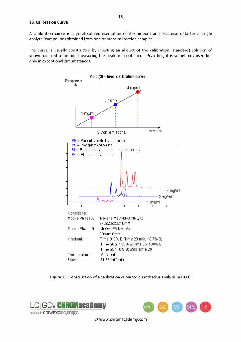
13. Calibration Curve

A calibration curve is a graphical representation of the amount and response data for a single analyte (compound) obtained from one or more calibration samples.

The curve is usually constructed by injecting an aliquot of the calibration (standard) solution of known concentration and measuring the peak area obtained. Peak height is sometimes used but only in exceptional circumstances.

Figure 15: Construction of a calibration curve for quantitative analysis in HPLC.

19


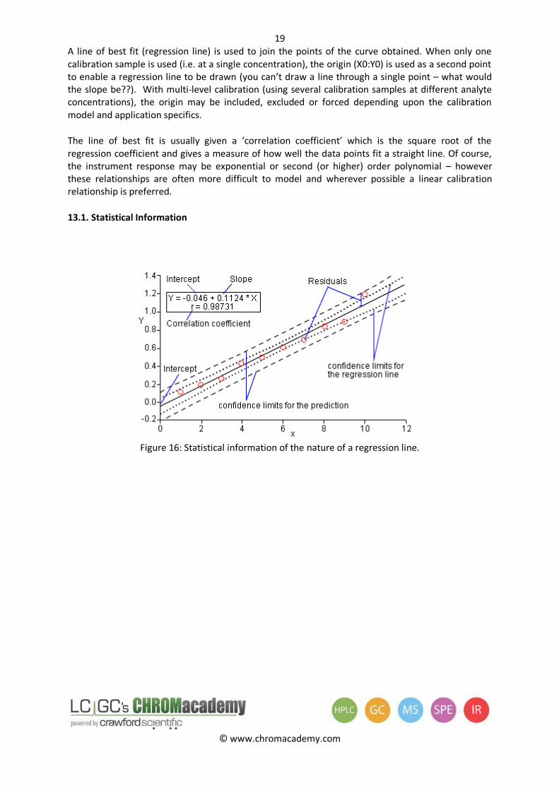
A line of best fit (regression line) is used to join the points of the curve obtained. When only one calibration sample is used (i.e. at a single concentration), the origin (X0:Y0) is used as a second point to enable a regression line to be drawn (you can’t draw a line through a single point – what would the slope be??). With multi-level calibration (using several calibration samples at different analyte concentrations), the origin may be included, excluded or forced depending upon the calibration model and application specifics.

The line of best fit is usually given a ‘correlation coefficient’ which is the square root of the regression coefficient and gives a measure of how well the data points fit a straight line. Of course, the instrument response may be exponential or second (or higher) order polynomial – however these relationships are often more difficult to model and wherever possible a linear calibration relationship is preferred.

13.1. Statistical Information

Figure 16: Statistical information of the nature of a regression line.

20


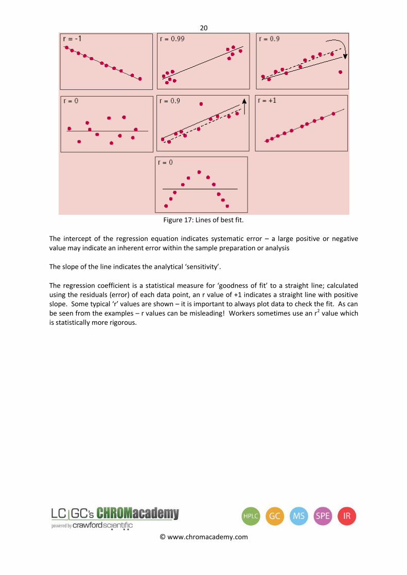
Figure 17: Lines of best fit.

The intercept of the regression equation indicates systematic error – a large positive or negative value may indicate an inherent error within the sample preparation or analysis

The slope of the line indicates the analytical ‘sensitivity’.

The regression coefficient is a statistical measure for ‘goodness of fit’ to a straight line; calculated using the residuals (error) of each data point, an r value of +1 indicates a straight line with positive slope. Some typical ‘r’ values are shown – it is important to always plot data to check the fit. As can be seen from the examples – r values can be misleading! Workers sometimes use an r2 value which is statistically more rigorous.

Various Values for the Regression Coefficient – care

must be taken when deciding if the instrument

response is linear!

21


14. External Standard Multi-Level Calibration

Multilevel calibration can be used when it is not sufficiently accurate to assume that a component shows a linear response or to confirm linearity of the calibration range.

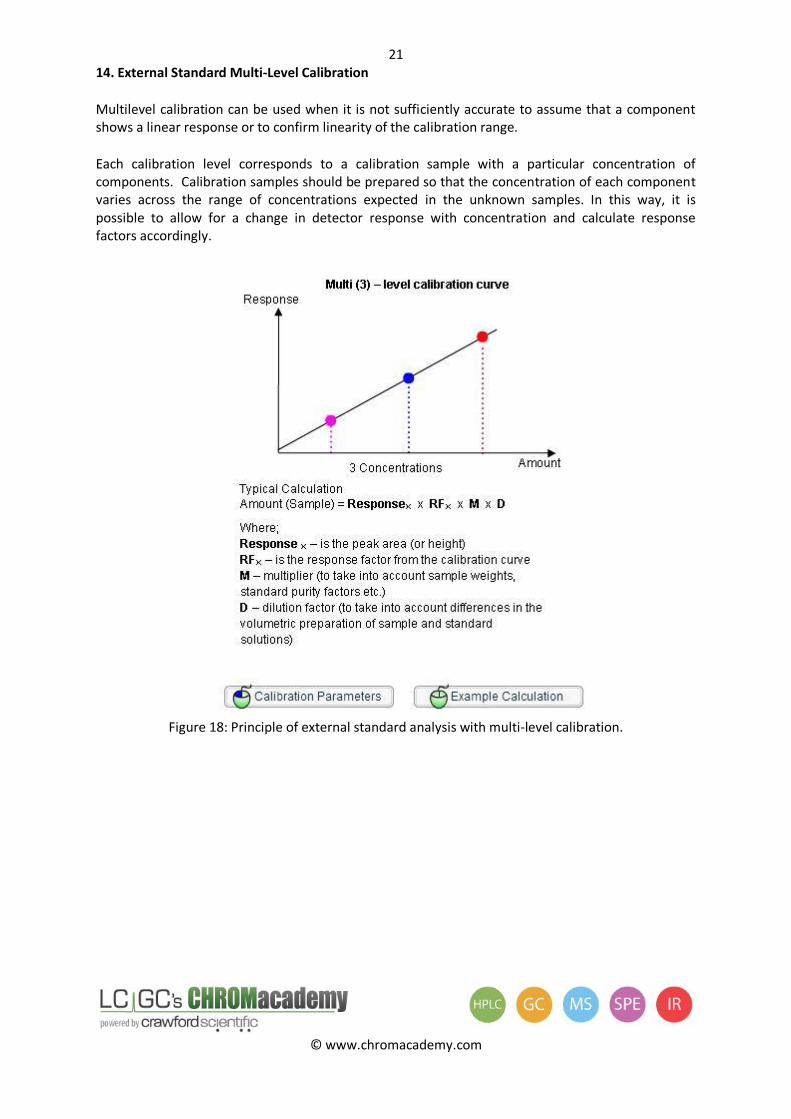
Each calibration level corresponds to a calibration sample with a particular concentration of components. Calibration samples should be prepared so that the concentration of each component varies across the range of concentrations expected in the unknown samples. In this way, it is possible to allow for a change in detector response with concentration and calculate response factors accordingly.

Figure 18: Principle of external standard analysis with multi-level calibration.

22


Example calculation:

An injection containing benzene at a concentration of 2,000 µg/mL is made and results in a peak area of 100,000.

The response factor for benzene:

An injection of the sample with the unknown concentration of benzene has a peak area of 57,000.

The amount of benzene present in the sample:

This multilevel calibration curve has three levels and shows a linear fit through the origin. This method of linear fit through the origin is similar to the single level calibration method. The detector response to concentration is assumed to be linear. The difference between the two calibration types is that, with multi-level calibration, the slope of the detector response can be determined by a best fit through a number of points, one for each level, and the regression coefficients used to substantiate the assumption of linearity.

Unknowns are determined in the same way as the single level calibration model – the difference is now that the method may be used to determine analyte concentrations over a wider range as the detector response has been calibrated with greater rigor.

Most data systems will allow the input of calculation variables to allow a ‘final result’ to be automatically calculated and printed.

23


14.1. Calibration Curve Information

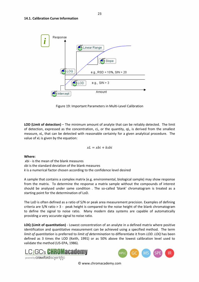
Figure 19: Important Parameters in Multi-Level Calibration

LOD (Limit of detection) – The minimum amount of analyte that can be reliably detected. The limit of detection, expressed as the concentration, cL, or the quantity, qL, is derived from the smallest measure, xL, that can be detected with reasonable certainty for a given analytical procedure. The value of xL is given by the equation:

Where: xbi - is the mean of the blank measures sbi is the standard deviation of the blank measures k is a numerical factor chosen according to the confidence level desired

A sample that contains a complex matrix (e.g. environmental, biological sample) may show response from the matrix. To determine the response a matrix sample without the compounds of interest should be analysed under same condition . The so-called ‘blank’ chromatogram is treated as a starting point for the determination of LoD.

The LoD is often defined as a ratio of S/N or peak area measurement precision. Examples of defining criteria are S/N ratio > 3 - peak height is compared to the noise height of the blank chromatogram to define the signal to noise ratio. Many modern data systems are capable of automatically providing a very accurate signal to noise ratio.

LOQ (Limit of quantitation) - Lowest concentration of an analyte in a defined matrix where positive identification and quantitative measurement can be achieved using a specified method. The term limit of quantitation is preferred to limit of determination to differentiate it from LOD. LOQ has been defined as 3 times the LOD (Keith, 1991) or as 50% above the lowest calibration level used to validate the method (US-EPA, 1986).

i

24


The LoQ is often defined as a ratio of S/N or peak area measurement precision and has much less stringent requirements than for limit of detection. Examples of defining criteria are S/N ratio > 20, or peak area precision better than 10%. The peak height is compared to the noise height of the blank chromatogram to define the signal to noise ratio. Many modern data systems are capable of automatically providing a very accurate signal to noise ratio.

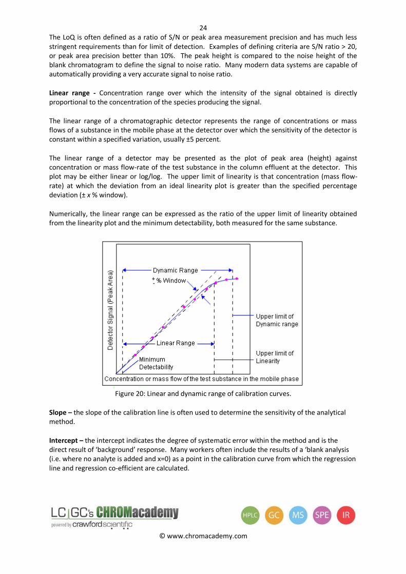
Linear range - Concentration range over which the intensity of the signal obtained is directly proportional to the concentration of the species producing the signal.

The linear range of a chromatographic detector represents the range of concentrations or mass flows of a substance in the mobile phase at the detector over which the sensitivity of the detector is constant within a specified variation, usually ±5 percent.

The linear range of a detector may be presented as the plot of peak area (height) against concentration or mass flow-rate of the test substance in the column effluent at the detector. This plot may be either linear or log/log. The upper limit of linearity is that concentration (mass flow-rate) at which the deviation from an ideal linearity plot is greater than the specified percentage deviation (± x % window).

Numerically, the linear range can be expressed as the ratio of the upper limit of linearity obtained from the linearity plot and the minimum detectability, both measured for the same substance.

Figure 20: Linear and dynamic range of calibration curves.

Slope – the slope of the calibration line is often used to determine the sensitivity of the analytical method.

Intercept – the intercept indicates the degree of systematic error within the method and is the direct result of ‘background’ response. Many workers often include the results of a ‘blank analysis (i.e. where no analyte is added and x=0) as a point in the calibration curve from which the regression line and regression co-efficient are calculated.

25


15. External Standard Multi-Level Calibration Curve - Typical Calculation

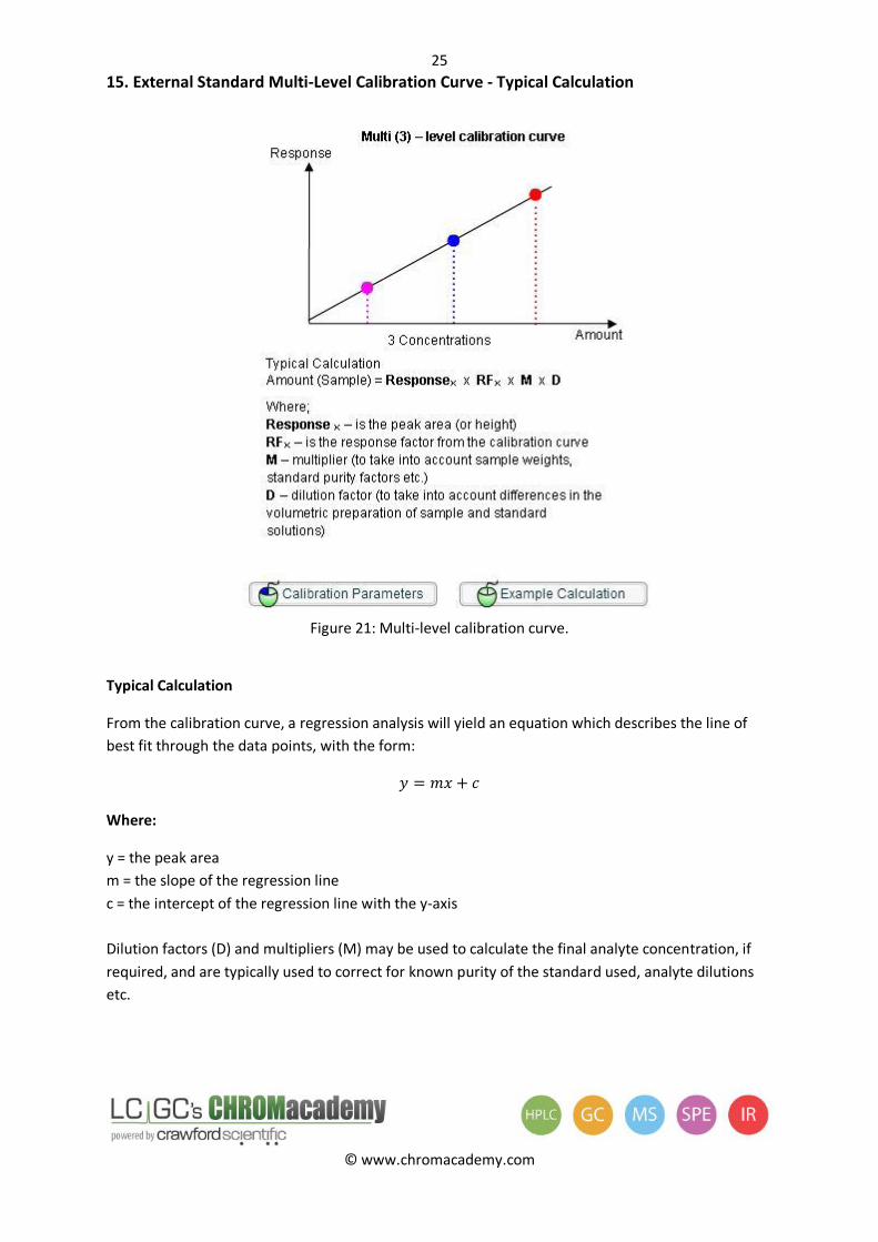
Figure 21: Multi-level calibration curve.

Typical Calculation

From the calibration curve, a regression analysis will yield an equation which describes the line of

best fit through the data points, with the form:

Where:

y = the peak area

m = the slope of the regression line

c = the intercept of the regression line with the y-axis

Dilution factors (D) and multipliers (M) may be used to calculate the final analyte concentration, if

required, and are typically used to correct for known purity of the standard used, analyte dilutions

etc.

26


Therefore, for a regression equation obtained from a multi-level calibration, such as that shown, the

equation of the best fit line is:

If a sample peak area of 327 units is obtained, the absolute amount of sample is calculated as

follows (solve for x = interpolated amount):

If the sample had been diluted from 10 mL to 25 mL during sample preparation then a dilution factor

(D) should be used. This is calculated as follows:

If a standard purity of 98.6% had previously been determined, then a multiplier (M) would be

required.

Therefore, the final amount of sample would be:

27


16. Internal Standard Analysis

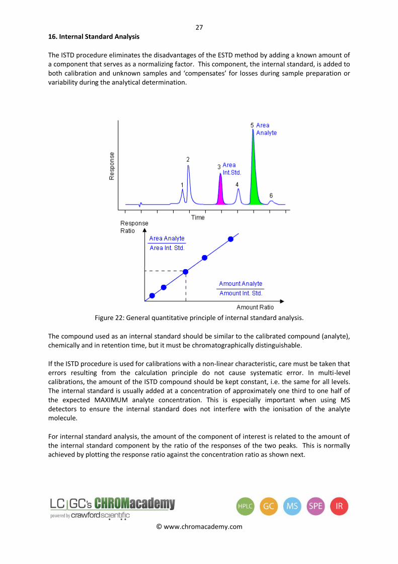
The ISTD procedure eliminates the disadvantages of the ESTD method by adding a known amount of a component that serves as a normalizing factor. This component, the internal standard, is added to both calibration and unknown samples and ‘compensates’ for losses during sample preparation or variability during the analytical determination.

Figure 22: General quantitative principle of internal standard analysis.

The compound used as an internal standard should be similar to the calibrated compound (analyte), chemically and in retention time, but it must be chromatographically distinguishable.

If the ISTD procedure is used for calibrations with a non-linear characteristic, care must be taken that errors resulting from the calculation principle do not cause systematic error. In multi-level calibrations, the amount of the ISTD compound should be kept constant, i.e. the same for all levels. The internal standard is usually added at a concentration of approximately one third to one half of the expected MAXIMUM analyte concentration. This is especially important when using MS detectors to ensure the internal standard does not interfere with the ionisation of the analyte molecule.

For internal standard analysis, the amount of the component of interest is related to the amount of the internal standard component by the ratio of the responses of the two peaks. This is normally achieved by plotting the response ratio against the concentration ratio as shown next.

28


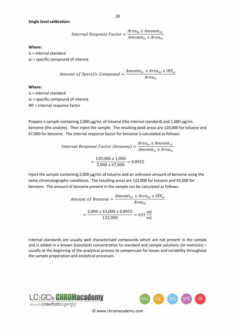
Single level calibration:

Where:

is = internal standard

sc = specific compound of interest

Where:

is = internal standard

sc = specific compound of interest

IRF = internal response factor

Prepare a sample containing 2,000 µg/mL of toluene (the internal standard) and 1,000 µg/mL

benzene (the analyte). Then inject the sample. The resulting peak areas are 120,000 for toluene and

67,000 for benzene. The internal response factor for benzene is calculated as follows:

Inject the sample containing 2,000 µg/mL of toluene and an unknown amount of benzene using the

same chromatographic conditions. The resulting areas are 122,000 for toluene and 43,000 for

benzene. The amount of benzene present in the sample can be calculated as follows:

Internal standards are usually well characterised compounds which are not present in the sample and is added in a known (constant) concentration to standard and sample solutions (or matrices) – usually at the beginning of the analytical process to compensate for losses and variability throughout the sample preparation and analytical processes.

29


Good internal standards:

elute near to, but are well resolved from, the analyte of interest

are chemically and physically similar to the analyte

are not present in the original sample mixture

are unreactive towards any of the sample components

are available in highly pure form

are added in the concentration range 0.3 – 0.5 of the expected MAXIMUM analyte concentration

It is often fairly difficult to fulfil all of these requirements for HPLC analysis. Often for MS detection, the internal standard will be an isotopically labelled version of the analyte, which can be spectrally rather than chromatographically resolved (i.e. the labelled version has a different mass than that analyte). Care must be taken when using this approach to avoid ion-suppression effects, which can serious affect the reproducibility of the analysis.

30


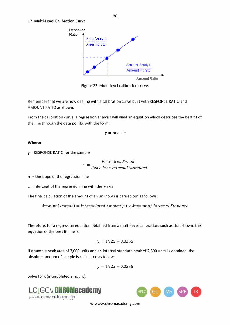
17. Multi-Level Calibration Curve

Figure 23: Multi-level calibration curve.

Remember that we are now dealing with a calibration curve built with RESPONSE RATIO and

AMOUNT RATIO as shown.

From the calibration curve, a regression analysis will yield an equation which describes the best fit of

the line through the data points, with the form:

Where:

y = RESPONSE RATIO for the sample

m = the slope of the regression line

c = intercept of the regression line with the y-axis

The final calculation of the amount of an unknown is carried out as follows:

Therefore, for a regression equation obtained from a multi-level calibration, such as that shown, the

equation of the best fit line is:

If a sample peak area of 3,000 units and an internal standard peak of 2,800 units is obtained, the

absolute amount of sample is calculated as follows:

Solve for x (interpolated amount).

31


REMEMBER

Therefore, the equation of the regression line becomes

Therefore the final amount, based on an internal standard mount of 0.110 units being added to the

sample solution would be:

Multipliers (M) and dilution factors (D) may also be included in the final calculation of the amount of

the sample, however, theses have been omitted here for clarity, but were included in the external

multi-level calibration curve (page 15).

theory of hplc quantitative and qualitative hplc

Documents