Generalized Uncertainty Principle and Angular Momentum

Pasquale Bosso∗ and Saurya Das†

Theoretical Physics Group and Quantum Alberta,Department of Physics and Astronomy, University of Lethbridge,

4401 University Drive, Lethbridge,Alberta, Canada, T1K 3M4

Abstract

Various models of quantum gravity suggest a modification of the Heisenberg’s Uncertainty Principle, to theso-called Generalized Uncertainty Principle, between position and momentum. In this work we show how thismodification influences the theory of angular momentum in Quantum Mechanics. In particular, we computePlanck scale corrections to angular momentum eigenvalues, the hydrogen atom spectrum, the Stern-Gerlachexperiment and the Clebsch-Gordan coefficients. We also examine effects of the Generalized Uncertainty Principleon multi-particle systems.

Contents

1 Introduction 2

2 Modified Angular Momentum Algebra 3

3 Modified Angular Momentum Spectrum 4

4 Modified Energy Levels of the Hydrogen Atom 6

5 Inclusion of a Magnetic Field 75.1 Uniform Magnetic Field . . . . . . . . . . . . . . . . . . . . . . . . . . . . . . . . . . . . . . . . . . . 85.2 Non-Uniform Magnetic Field: Stern-Gerlach Experiment . . . . . . . . . . . . . . . . . . . . . . . . . 8

6 Multi-Particles Systems 106.1 Dependence of [Li, Lj ] on the number of particles . . . . . . . . . . . . . . . . . . . . . . . . . . . . . 106.2 Addition of Angular Momentum . . . . . . . . . . . . . . . . . . . . . . . . . . . . . . . . . . . . . . 116.3 Clebsch-Gordan Coefficients . . . . . . . . . . . . . . . . . . . . . . . . . . . . . . . . . . . . . . . . . 12

6.3.1 Orthogonality relations . . . . . . . . . . . . . . . . . . . . . . . . . . . . . . . . . . . . . . . 136.3.2 Clebsch-Gordan Recursion Relation . . . . . . . . . . . . . . . . . . . . . . . . . . . . . . . . 136.3.3 Clebsch-Gordan Coefficient Tables . . . . . . . . . . . . . . . . . . . . . . . . . . . . . . . . . 14

7 Conclusions 15

Appendix A GUP modified angular momentum commutator 16

Appendix B Clebsch-Gordan Coefficients 17B.1 L = Lmax, M = Lmax . . . . . . . . . . . . . . . . . . . . . . . . . . . . . . . . . . . . . . . . . . . . 17B.2 M = Lmax − 1 . . . . . . . . . . . . . . . . . . . . . . . . . . . . . . . . . . . . . . . . . . . . . . . . 17

B.2.1 L = Lmax . . . . . . . . . . . . . . . . . . . . . . . . . . . . . . . . . . . . . . . . . . . . . . . 17B.2.2 L = Lmax − 1 . . . . . . . . . . . . . . . . . . . . . . . . . . . . . . . . . . . . . . . . . . . . . 18

B.3 M = Lmax − 2 . . . . . . . . . . . . . . . . . . . . . . . . . . . . . . . . . . . . . . . . . . . . . . . . 18

∗pasquale.bosso@uleth.ca†saurya.das@uleth.ca

1

arX

iv:1

607.

0108

3v5

[gr

-qc]

7 J

un 2

017

B.3.1 L = Lmax . . . . . . . . . . . . . . . . . . . . . . . . . . . . . . . . . . . . . . . . . . . . . . . 18B.3.2 L = Lmax − 1 . . . . . . . . . . . . . . . . . . . . . . . . . . . . . . . . . . . . . . . . . . . . . 19B.3.3 L = Lmax − 2 . . . . . . . . . . . . . . . . . . . . . . . . . . . . . . . . . . . . . . . . . . . . . 19

1 Introduction

A successful formulation of a quantum theory of gravity, and its possible unification with the other fundamentalinteractions of Nature, remains as one of the foremost challenges of theoretical physics. While various promisingapproaches for a Quantum Gravity (QG) theory have been proposed, such as Superstring Theory, Loop QuantumGravity, etc., there has not been a single experiment or observation to our knowledge, which clearly supports orrefutes any theory. On the other hand, no experiment or observation has shown any deviation from the presenttheory of gravity. Although this is normally attributed to the immensity of, and the related difficulty of directlyaccessing the Planck energy scale (EPl ∼ 1016 TeV), there are indications that current experimental accuracies andthose in the near future may be sufficient to detect such experimental signatures in at least some laboratory basedexperiments.

In the last couple of decades, it has been shown that most theories of QG predict momentum dependentmodifications of the position-momentum commutation relation, the consequent modifications of the Heisenberg’sUncertainty Principle (HUP), and existence of a minimum measurable length near the Planck scale [1–7]. Studiesof the so-called Generalized Uncertainty Principle (GUP) showed modifications in several areas of Quantum Me-chanics (QM). For example, modifications are expected for the Hamiltonian describing a minimal coupling with anelectromagnetic field, as shown in [8]. This result was then used to show modification of the Landau levels [8, 9].It is possible to show that GUP affects also Lamb shift, the case of a potential step and of a potential barrier, aquantum configuration used in Scanning Tunnelling Microscopes [8,9], the case of a particle in a box [10], showingthat the length of the box is quantized when a GUP is considered, and the energy levels for a simple harmonicoscillator [9]. It has also been showed that GUP can also be detected considering its effects on quantum opticalsystems [11].

Carrying forward this program, in this article we compute QG corrections to an important theoretical as wellas experimental area of quantum mechanics, namely the angular momentum of elementary quantum systems,and their experimental applications. We indeed show that there are potential measurable Planck scale effects towell-understood phenomena such as line spectra from the hydrogen atom, the Stern-Gerlach experiment, Larmorfrequency and Clebsh-Gordan coefficients.

Several models were proposed in the past years to account for this modification of the Heisenberg principle. Aquadratic model, for example, proposed in [5,7,12], can account for this feature by adding a momentum dependentquadratic term in the position-momentum commutation relation. In what follows, we will consider the most generalcommutation relation correct up to second order in momentum [9]

[xi, pj ] = i~[δij − α

(pδij +

pipjp

)+ β2(p2δij + 3pipj)

], (1)

where α = α0/MP c, β = β0/MP c, α0 and β0 are dimensionless parameters, normally assumed to be of order unity,and MP ∼ 2 × 10−8 Kg is the Planck Mass, while i, j = 1, 2, 3 represent different vector components. One alsoassumes that position commutes with position, and momentum with momentum

[xi, xj ] = 0 = [pi, pj ] . (2)

This assumption implies the fulfillment of Jacobi identity, as shown in [9]. The Jacobi identity in the context ofGUP was also studied in [13]. The quadratic model can be obtained by setting the linear term in (1) to zero. Inthis work, we will consider the case α = β. The case α 6= β can be easily obtained following the same steps ofthis present paper. In a one-dimensional problem, using the modified commutation relation, one can obtain thefollowing inequality between uncertainties

∆x∆p ≥ ~2

[1− 2α〈p〉+ 4β2〈p2〉] =

≥ ~2

[1 +

(α√〈p2〉

+ 4β2

)∆p2 + 4β2〈p〉2 − 2α

√〈p2〉

].

(3)

Since the existence of a minimal measurable length implies the existence of a minimal angular resolution, we areforced to consider a GUP also for angle variables and their conjugate momenta, i.e., angular momenta. We therefore

2

expect a modification of the angular momentum algebra. In the present paper we will obtain this modification asa consequence of the GUP in position and momentum.

This paper is organized as follows. In Section 2 we first present the modified angular momentum algebra andsome useful relations for subsequent sections. In Section 3 we will show how the angular momentum spectrum ismodified, illustrating some issues and assumptions made to solve them. In Section 4 we will apply our results tothe hydrogen atom. In Section 5 we will consider magnetic interaction on an atom. This interaction is relevantbecause, as described in Subsection 5.2, a direct observation of GUP effects in a Stern-Gerlach-like experimentmay be possible. In Section 6 we study systems composed of more than one particle, while in Subsection 6.3 weintroduce the modified Clebsch-Gordan coefficients in GUP. Finally, in Section 7 we summarize our results, list theopen problems and discuss future directions.

2 Modified Angular Momentum Algebra

In this section we start with the standard definition of angular momentum in Classical Mechanics,

~L = ~q × ~p =

ypz − zpyzpx − xpzxpy − ypx

. (4)

GUP now implies the existence of minimal measurable angles. Using the commutator (1), one can show (seeAppendix A) that the commutation relation between angular momentum components is modified as

[Li, Lj ] = i~εijkLk(1− αp+ α2p2) . (5)

It is also possible to show that Jacobi identity is trivially fulfilled by this modified commutation relation. Note thatwe recover the standard commutation relation [Li, Lj ] = i~εijkLk for α = 0. Including GUP, one still has however

[L2, Lj ] = 0 . (6)

Therefore, even with a modified angular momentum algebra, we can define simultaneous eigenstates of L2 and Lz.Furthermore we notice that, since for (112) and (115) in Appendix A also p and p2 commute with Lz, they alsocommute with L2

[L2, p] =∑

i=1,2,3

Li[Li, p] + [Li, p]Li = 0 , [L2, p2] =∑

i=1,2,3

Li[Li, p2] + [Li, p

2]Li = 0 . (7)

Thus we can define simultaneous eigenstates of the operators L2, Lz, and p, and moreover, such a state is also anenergy eigenstate for the free case.

As proposed in [9], we will also expand the momentum operator p, subject to the modified commutation relation(1), in terms of a low-energy momentum operator p0, subject to the standard commutation relation, up to secondorder in α. The following relation is exact, such that (1) is satisfied, as shown in [9] 1

pi = p0,i(1− αp0 + 2α2p20), where p0,i = −i~ ∂

∂qi. (8)

This expansion is sufficient to satisfy (1). It also gives us the necessary tool to compute GUP corrections to thequantum mechanical systems in what follows. Notice that ~p0 corresponds to the generator of translations. On theother hand, introducing the generators of rotations, one necessarily obtains

[L0,i, L0,j ] = i~εijkL0,k , (9)

and we can obtain an expansion of the physical angular momentum in terms of generators of translations androtations

Li = L0,i(1− αp0 + 2α2p20) . (10)

Using this expansion, we find

[Li, Lj ] = [L0,i, L0,j ](1− αp0 + 2α2p20)2 = i~εijkL0,k(1− 2αp0 + 5α2p20) = i~εijkLk(1− αp+ α2p2) . (11)

We note that now the angular momentum does not coincide with the generator of rotations, and is thereforenot conserved in general even for rotationally invariant Hamiltonians. However, ~L can be expanded in terms ofgenerators of rotations and translations.

1As seen in Section 4 of this paper, this relation poses no problem of analyticity for one effective spatial dimension, e.g. r. For higherdimensions, the problem is circumvented by considering the Dirac equation [14,15].

3

3 Modified Angular Momentum Spectrum

As mentioned above, we consider simultaneous eigenstates

L2|pλm〉 = ~2λ|pλm〉 λ ≥ 0 , (12a)

Lz|pλm〉 = ~m|pλm〉 m2 ≤ λ . (12b)

and define as usual

L+ = Lx + iLy , L− = Lx − iLy . (13)

Using (5), we get

[Lz, L+] = [Lz, Lx] + i[Lz, Ly] = ~(iLy + Lx)(1− αp+ α2p2) = ~L+(1− C) , (14a)

[Lz, L−] = [Lz, Lx]− i[Lz, Ly] = ~(iLy − Lx)(1− αp+ α2p2) = −~L−(1− C) , (14b)

[L2, L+] = [L2, Lx] + i[L2, Ly] = 0 , (14c)

[L2, L−] = [L2, Lx]− i[L2, Ly] = 0 , (14d)

[L+, L−] = [Lx, Lx]− i[Lx, Ly] + i[Ly, Lx] + [Ly, Ly] = −2i[Lx, Ly] = 2~Lz(1− C) . (14e)

where C ≡ αp− α2p2 represents the modification due to the GUP. From (14c, 14d) we obtain

L2L±|pλm〉 = L±L2|pλm〉 = ~2λL±|pλm〉 . (15)

Thus, even for GUP, the ladder operators do not change the eigenvalues of the magnitude of the angular momentum.On the other hand, using (14a, 14b), we get

LzL±|pλm〉 = L±[Lz ± (1− C)]|pλm〉 = ~[m± (1− C)]L±|pλm〉 . (16)

That is, while L± still act as ladder operators, the spacing between two consecutive Lz eigenstates undergoesmodifications due to GUP. Further, from (13) and (5) we get

L−L+ = L2 − Lz[Lz + ~(1− C)] , L+L− = L2 − Lz[Lz − ~(1− C)] , (17)

from which one gets the norms of the states L±|pλm〉 as

||L±|pλm〉||2 = 〈pλm|L∓L±|pλm〉 = ~2λ−m[m± (1− C)] ≥ 0 . (18)

We note that if we considered eigenstates of L2 and Lz alone, we would have obtained

||L±|λm〉||2 = 〈λm|L∓L±|λm〉 = ~2λ−m[m± (1− 〈C〉)] ≥ 0 , (19)

that is, the modification due to the GUP would appear as 〈C〉. This observation will come in handy when we willconsider GUP effects for the hydrogen atom model in Sec. 4. Also, notice that 1−〈C〉 is a positive quantity. Indeed,since

(∆p)2 = 〈p2〉 − 〈p〉2 ≥ 0 ⇒ 〈p2〉 ≥ 〈p〉2 , (20)

one can write1− 〈C〉 ≥ α2〈p〉2 − α〈p〉+ 1 > 0 ∀〈p〉 ∈ R . (21)

Since m2 ≤ λ, there are upper and lower bounds on m, which we denote m+ and m−, respectively. From (18),it follows

L±|pλm±〉 = 0⇒ λ = m±[m± ± (1− C)] . (22)

We can reach these values starting from any value m and applying s times L+ or t times L−, with s, t ∈ N

m+ =m+ s(1− C) , m− =m− t(1− C) . (23)

Combining these two relations we find

m+ = m− + (s+ t)(1− C) = m− + η(1− C) , (24)

4

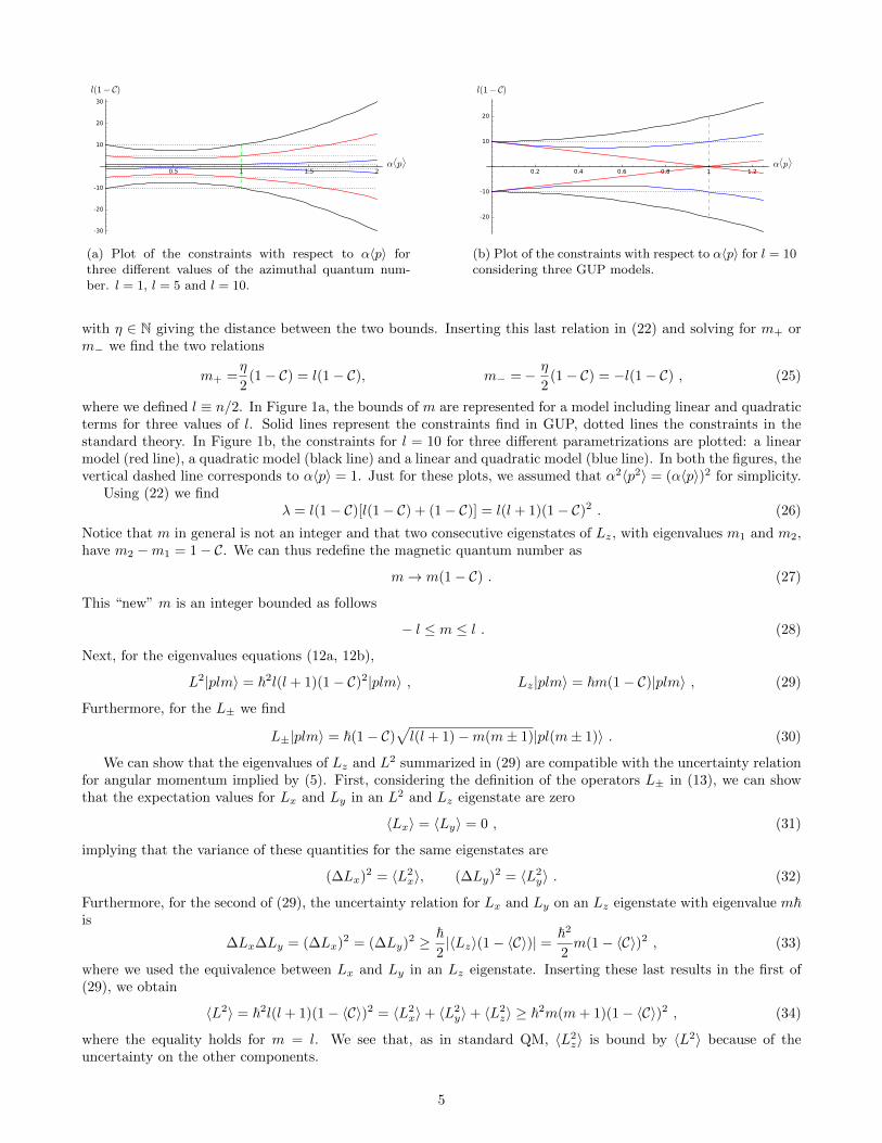
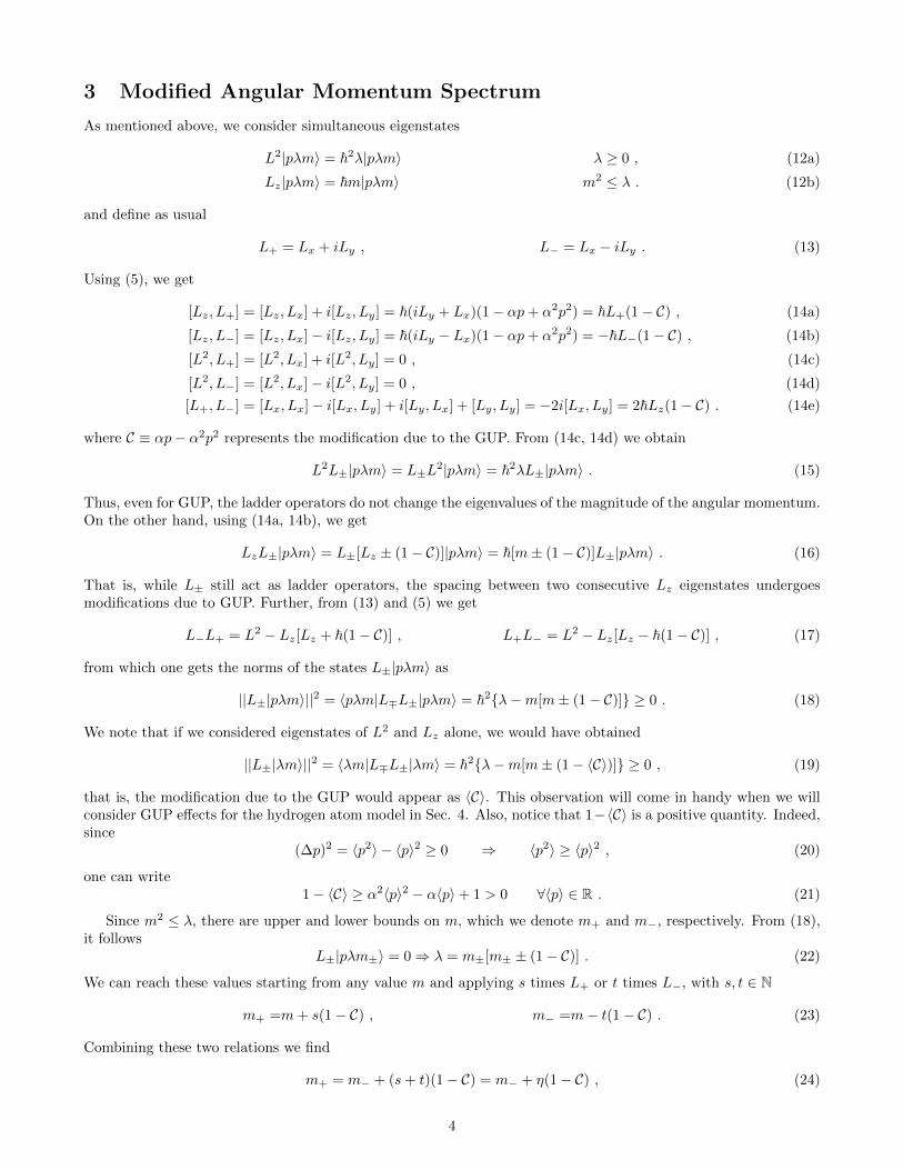
(a) Plot of the constraints with respect to α〈p〉 forthree different values of the azimuthal quantum num-ber. l = 1, l = 5 and l = 10.

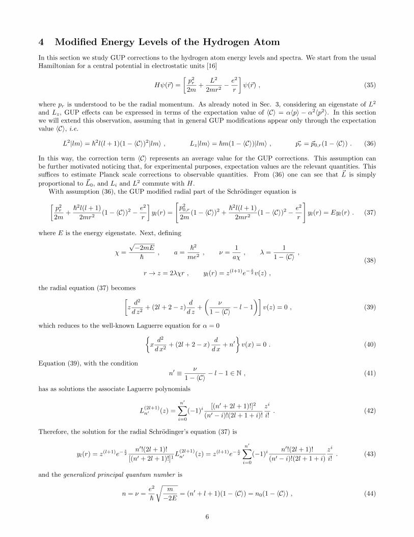
(b) Plot of the constraints with respect to α〈p〉 for l = 10considering three GUP models.

with η ∈ N giving the distance between the two bounds. Inserting this last relation in (22) and solving for m+ orm− we find the two relations

m+ =η

2(1− C) = l(1− C), m− =− η

2(1− C) = −l(1− C) , (25)

where we defined l ≡ n/2. In Figure 1a, the bounds of m are represented for a model including linear and quadraticterms for three values of l. Solid lines represent the constraints find in GUP, dotted lines the constraints in thestandard theory. In Figure 1b, the constraints for l = 10 for three different parametrizations are plotted: a linearmodel (red line), a quadratic model (black line) and a linear and quadratic model (blue line). In both the figures, thevertical dashed line corresponds to α〈p〉 = 1. Just for these plots, we assumed that α2〈p2〉 = (α〈p〉)2 for simplicity.

Using (22) we findλ = l(1− C)[l(1− C) + (1− C)] = l(l + 1)(1− C)2 . (26)

Notice that m in general is not an integer and that two consecutive eigenstates of Lz, with eigenvalues m1 and m2,have m2 −m1 = 1− C. We can thus redefine the magnetic quantum number as

m→ m(1− C) . (27)

This “new” m is an integer bounded as follows

− l ≤ m ≤ l . (28)

Next, for the eigenvalues equations (12a, 12b),

L2|plm〉 = ~2l(l + 1)(1− C)2|plm〉 , Lz|plm〉 = ~m(1− C)|plm〉 , (29)

Furthermore, for the L± we find

L±|plm〉 = ~(1− C)√l(l + 1)−m(m± 1)|pl(m± 1)〉 . (30)

We can show that the eigenvalues of Lz and L2 summarized in (29) are compatible with the uncertainty relationfor angular momentum implied by (5). First, considering the definition of the operators L± in (13), we can showthat the expectation values for Lx and Ly in an L2 and Lz eigenstate are zero

〈Lx〉 = 〈Ly〉 = 0 , (31)

implying that the variance of these quantities for the same eigenstates are

(∆Lx)2 = 〈L2x〉, (∆Ly)2 = 〈L2

y〉 . (32)

Furthermore, for the second of (29), the uncertainty relation for Lx and Ly on an Lz eigenstate with eigenvalue m~is

∆Lx∆Ly = (∆Lx)2 = (∆Ly)2 ≥ ~2|〈Lz〉(1− 〈C〉)| =

~2

2m(1− 〈C〉)2 , (33)

where we used the equivalence between Lx and Ly in an Lz eigenstate. Inserting these last results in the first of(29), we obtain

〈L2〉 = ~2l(l + 1)(1− 〈C〉)2 = 〈L2x〉+ 〈L2

y〉+ 〈L2z〉 ≥ ~2m(m+ 1)(1− 〈C〉)2 , (34)

where the equality holds for m = l. We see that, as in standard QM, 〈L2z〉 is bound by 〈L2〉 because of the

uncertainty on the other components.

5

4 Modified Energy Levels of the Hydrogen Atom

In this section we study GUP corrections to the hydrogen atom energy levels and spectra. We start from the usualHamiltonian for a central potential in electrostatic units [16]

Hψ(~r) =

[p2r2m

+L2

2mr2− e2

r

]ψ(~r) , (35)

where pr is understood to be the radial momentum. As already noted in Sec. 3, considering an eigenstate of L2

and Lz, GUP effects can be expressed in terms of the expectation value of 〈C〉 = α〈p〉 − α2〈p2〉. In this sectionwe will extend this observation, assuming that in general GUP modifications appear only through the expectationvalue 〈C〉, i.e.

L2|lm〉 = ~2l(l + 1)(1− 〈C〉)2|lm〉 , Lz|lm〉 = ~m(1− 〈C〉)|lm〉 , ~pr = ~p0,r(1− 〈C〉) . (36)

In this way, the correction term 〈C〉 represents an average value for the GUP corrections. This assumption canbe further motivated noticing that, for experimental purposes, expectation values are the relevant quantities. Thissuffices to estimate Planck scale corrections to observable quantities. From (36) one can see that ~L is simply

proportional to ~L0, and Li and L2 commute with H.With assumption (36), the GUP modified radial part of the Schrodinger equation is[p2r2m

+~2l(l + 1)

2mr2(1− 〈C〉)2 − e2

r

]yl(r) =

[p20,r2m

(1− 〈C〉)2 +~2l(l + 1)

2mr2(1− 〈C〉)2 − e2

r

]yl(r) = Eyl(r) . (37)

where E is the energy eigenstate. Next, defining

χ =

√−2mE

~, a =

~2

me2, ν =

1

aχ, λ =

1

1− 〈C〉,

r → z = 2λχr , yl(r) = z(l+1)e−z2 v(z) ,

(38)

the radial equation (37) becomes[zd2

d z2+ (2l + 2− z) d

d z+

(ν

1− 〈C〉− l − 1

)]v(z) = 0 , (39)

which reduces to the well-known Laguerre equation for α = 0xd2

d x2+ (2l + 2− x)

d

d x+ n′

v(x) = 0 . (40)

Equation (39), with the condition

n′ ≡ ν

1− 〈C〉− l − 1 ∈ N , (41)

has as solutions the associate Laguerre polynomials

L(2l+1)n′ (z) =

n′∑i=0

(−1)i[(n′ + 2l + 1)!]2

(n′ − i)!(2l + 1 + i)!

zi

i!. (42)

Therefore, the solution for the radial Schrodinger’s equation (37) is

yl(r) = z(l+1)e−z2

n′!(2l + 1)!

[(n′ + 2l + 1)!]1L(2l+1)n′ (z) = z(l+1)e−

z2

n′∑i=0

(−1)in′!(2l + 1)!

(n′ − i)!(2l + 1 + i)

zi

i!. (43)

and the generalized principal quantum number is

n = ν =e2

~

√m

−2E= (n′ + l + 1)(1− 〈C〉) = n0(1− 〈C〉) , (44)

6

where n0 is the principal quantum number of the standard theory. In conclusion, the GUP modified energy levelsof the hydrogen atom are given by

En = − e4

~2m

2[(n′ + l + 1)(1− 〈C〉)]2= −

(e2

~c

)2mc2

2n2' En(0)[1 + 2α〈p0〉+ α2(3〈p20〉 − 4〈p0〉2)] , (45)

where En(0) is the corresponding energy level of the standard theory and where 〈p0〉 and 〈p20〉 are the expectationvalues of p0 and p20 in a |n0lm〉 eigenstate. As before, we recover the results of the standard theory of the hydrogenatom for α = 0.

Eq. (45) also implies that the wavenumber of photons emitted when the atom transits from an energy level Ei

to Ef changes as follows

1

λ=Ei − Ef

hc= R∞

[1

n20,f (1− 〈Cf 〉)2− 1

n20,i(1− 〈Ci〉)2

], (46)

where R∞ is the Rydberg constant. We see now that the GUP-corrected spectrum depends not only on the principalquantum number, but also on the expectation values of the electron’s momentum, as well as its angular momentumquantum numbers (the latter as we know also happens for the relativistic hydrogen atom).

5 Inclusion of a Magnetic Field

Since a magnetic field interacts with the angular momentum of an atom via its magnetic moment, we expect thatGUP modifications of the angular momentum theory will result in a modification of this interaction and haveobservable consequences. In what follows we will consider atoms with only one electron in an S shell (l = 0) and allother levels being filled. Examples for these kind of atoms are those of the first group of the periodic table and theelements in the group of copper. This may allow us to test the direct consequences of GUP on angular momentastudying its effects on the electronic spin.

We assume the spin operators to satisfy the same modified algebra for the angular momentum (5) and the same“low energy” expansion (10). The magnetic moment of an electron is

~M = −gSµB

~~S , (47)

where

µB =e~2m

, (48)

is the Bohr magneton, gS is the electron g-factor and ~S is the spin operator. Therefore we set

~M = ~M0(1− αp0 + 2α2p20) , (49)

where~M0 = −gSµB

~~S0 , (50)

satisfying the standard algebra, is interpreted as the magnetic moment at low energies.For magnetic fields less than ∼ 106 T [17], the quadrupole term appearing in the Hamiltonian for the magnetic

interaction on an atomic system is negligible with respect the dipole term. Therefore, we can write the Hamiltonianconsidering only a term involving the scalar product between the magnetic moment and the magnetic field itself

H =p2

2m− ~M · ~B . (51)

Using (8) and (49), we can rewrite this relation in terms of low-energy quantities

H =p202m

(1− 2αp0 + 5α2p20)− (1− αp0 + 2α2p20) ~M0 · ~B . (52)

Looking at the second term, i.e. (1 − αp0 + 2α2p20) ~M0 · ~B, we notice that it acts on both the space and the spin

variables through the operators p0 and ~M0 respectively. As in the previous section, we replace p0 and p20 with 〈p0〉and 〈p20〉, respectively. In this way, the wavefunction can be factorized in its space and spin parts as follows

Ψ(~r, t) = ψ(~r, t)[α(t)|+〉+ β(t)|−〉] , (53)

7

with ψ the spatial wave function, α and β functions of time such that |α|2 + |β|2 = 1, and |+〉 and |−〉 eigenstatesof the z-component of the magnetic moment operator

Mz|+〉 = µ0|+〉 , Mz|−〉 = −µ0|−〉 . (54)

Therefore the Schrodinger’s equation also splits into

i~∂

∂tψ(~r, t) =

p202m

(1− 〈C〉)2ψ(~r, t) , (55a)

i~d

d t(α(t)|+〉+ β(t)|−〉) = − ~M0 · ~B(1− 〈C〉)(α(t)|+〉+ β(t)|−〉) . (55b)

We now show how this modification affects the magnetic interaction and how it could in principle be tested.

5.1 Uniform Magnetic Field

First we consider a uniform magnetic field along the z-axis, with the atom moving along the y-axis. Eq. (55b) foreach component of the spinor can therefore be written as

i~d

d tα(t) = −µ0B(1− 〈C〉)α(t) , (56a)

i~d

d tβ(t) = µ0B(1− 〈C〉)β(t) , (56b)

from which one can find the modified Larmor frequency of the system

ωL = −2µ0B

~(1− 〈C〉) . (57)

Furthermore, since the magnitude of the linear momentum is not changed by the magnetic field, we can obtain thesame form for the equations of motion as found in the standard theory

d

d t〈 ~M〉 = ~Ω× 〈 ~M〉 , (58)

where ~Ω = ωLuz. We therefore see that the Larmor frequency is modified by the GUP, although the form of theprecession equation remains unchanged.

5.2 Non-Uniform Magnetic Field: Stern-Gerlach Experiment

In this subsection we will study the effects of GUP on the Stern-Gerlach experiment.Consider a magnetic field with a gradient along the z-direction [18]

~B(~r) = Bz(~r)uz − b′xux, where Bz(~r) = B0 + b′z , (59)

with b′∆z B0, where ∆z is the width of the beam used for the experiment along the z-axis. The term −b′xux isnecessary to ensure ~∇ · ~B = 0. If the dominant part of the field along z is much more intense that the transversecomponent over the transverse extension of the wave packet, that is

〈Mz〉Bz ' 〈Mz〉B0 〈Mx〉b′∆x , (60)

then the eigenstates of − ~M · ~B remain practically equal to |±〉z, since we can use the approximation ~M · ~B 'MzBz,and we can neglect the transverse component. For the original Stern-Gerlach experiment [19] one has the followingvalues

B0 ' 0.1 T , b′ ' 1 T/mm , ∆z ' ∆x ' 0.03 mm , (61)

that isB0

b′∆x' 1

0.3. (62)

8

With this assumption, the Schrodinger’s equation for the two spin component is

i~∂

∂tψ± =

[p202m

(1− 〈C〉)2 ∓ µ0(B0 + b′z)(1− 〈C〉)]ψ± . (63)

The expectation values of the position and of the momentum are given by

〈~r±〉 =

∫~r|ψ±(~r, t)|2d3r∫|ψ±(~r, t)|2d3r

, 〈~p±〉 =

∫ψ∗±(~r, t)~pψ±(~r, t)d3r∫|ψ±(~r, t)|2d3r

= 〈~p0±〉(1− 〈C〉) . (64)

Consider the following set of equations derived from the Ehrenfest’s Theorem

d

dt〈~r±〉 =

〈~p±〉m

=〈~p0±〉m

(1− 〈C〉) , (65a)

d

dt〈px±〉 = −

⟨∓ ∂

∂xµ0B(1− 〈C〉)

⟩= 0 , (65b)

d

dt〈py±〉 = −

⟨∓ ∂

∂yµ0B(1− 〈C〉)

⟩= 0 , (65c)

d

dt〈pz±〉 = −

⟨∓ ∂

∂zµ0B(1− 〈C〉)

⟩= ±µ0b

′(1− 〈C〉) . (65d)

We assume that at t = 0 a beam of atoms enters the apparatus, which we assume to be the origin of the coordinatesystem. We also assume that the initial momentum is directed along the y-axis, without any component along thex or z-axis, that is

〈x±〉(0) = 〈y±〉(0) = 〈z±〉(0) = 0 , (66a)

〈px±〉(0) = 〈pz±〉(0) = 0 , (66b)

〈py±〉(0) = mv . (66c)

We then obtain the following equations for its motion

〈x±〉(t) = 0 , (67a)

〈y±〉(t) = vt , (67b)

〈z±〉(t) = ±µ0b′t2

2m(1− 〈C〉) . (67c)

As for the standard theory, these equations represent a beam splitting in two along the z-axis. In this case,though, the term 〈C〉 will impose a dependence of the splitting on the expectation values of the momentum and themomentum squared of the electron in the outer S shell, the splitting being

δz =µ0b′

m

L2

v2(1− 〈C〉) , (68)

where L is the length of the apparatus.Again, for the Stern-Gerlach apparatus described in [19], one has for an electron in the state 5S state of silver

atoms

〈p20〉 = 2.83× 10−26 N2s2 , 〈p0〉 = 0 Ns . (69)

We have that the ratio between the expected splitting in GUP and the splitting in the standard theory is

δzGUP

δz0− 1 = −〈C〉 =

α20〈p20〉

(MP c)2' α2

06.66× 10−28 . (70)

For splittings of the order achieved in the original experiment (∼ 0.2 mm), the difference between the GUP andthe standard cases would not be observable. But if larger splittings could be produced, for example with a longerapparatus or lower velocities of the atoms in the beam, a better resolution would be achieved. On the other hand,one could also use atoms other than silver. In the model used to describe the Stern-Gerlach experiment, though, avariation of the mass leads to two contrasting effects. Consider for example, atoms heavier than silver. Since theinverse of the mass appears in (68), this will reduce the separation of the two spots. On the other hand, higheratomic numbers lead to higher momenta for the external electrons, and hence to higher |〈C〉|. The two effects willthus compete with each other.

9

6 Multi-Particles Systems

In this section we will examine how GUP affects multiparticle angular momentum algebra.

6.1 Dependence of [Li, Lj] on the number of particles

Consider a system of N particles with angular momentum ~ln, with n = 1, . . . , N , and the total angular momentum

~L =

N∑n=1

~ln . (71)

The commutator between components of the total angular momentum is

[Li, Lj ] =

N∑n=1

N∑m=1

[li,n, lj,m] =

N∑n=1

[li,n, lj,n] =

N∑n=1

i~εijklk,n(1− αpn + α2p2n)

= i~εijk[Lk −N∑

n=1

lk,n(αpn − α2p2n)] =

= i~εijk

[Lk(1− αP + α2P 2)− α

N∑n=1

(lk,npn −

LkP

N

)+ α2

N∑n=1

(lk,np

2n −

LkP2

N

)], (72)

where

P 2 =

N∑n=1

[p2n + 2

N−1∑m>n

~pn · ~pm

], (73)

and where we assumed[li,m, lj,n] = 0 , m 6= n , (74)

i.e. the angular momentum components of different particles commute.Consider for example the case in which all the particles in the system have the same angular momentum, e.g.

particle in a rotating ring,

ln,k =Lk

N, n = 1, . . . , N , (75)

in which case from (72), one obtains

[Li, Lj ] = i~εijkLk

[1− αP + α2P 2 − α

N

N∑n=1

(pn − P ) +α2

N

N∑n=1

(p2n − P 2

)]. (76)

As a second example, we consider particles with the same linear momentum, e.g., a rigid body in pure translation,for which

pn =P

N, n = 1, . . . , N , (77)

in which case we find

[Li, Lj ] = i~εijk

[Lk(1− αP + α2P 2)− α

NP

N∑n=1

(lk,n − Lk) +α2

N2P 2

N∑n=1

(lk,n −NLk)

]=

= i~εijkLk

(1− α

NP +

α2

N2P 2

). (78)

GUP in multiparticle system was also considered in [20]. Note that the RHS of (76) and (78) scale as differentpowers of N .

10

6.2 Addition of Angular Momentum

In this subsection we examine the problem of addition of angular momentum including GUP.Consider a system composed by N particles, with ln and mn the azimuthal and magnetic quantum numbers of

the particles, with n = 1, . . . , N . From (29) we have

l2n|ln,mn〉 = ~2(1− 〈Cn〉)2ln(ln + 1)|ln,mn〉 , (79a)

ln,z|ln,mn〉 = ~(1− 〈Cn〉)mn|ln,mn〉 . (79b)

The z-component of the angular momentum for the composite system is

Lz =

N∑n=1

ln,z . (80)

Operating on the combined state

|ln,mn〉 =

N⊗n=1

|ln,mn〉 , (81)

we obtain

Lz|ln,mn〉 =

N∑n=1

ln,z|ln,mn〉 =

N∑n=1

~(1− 〈Cn〉)mn|ln,mn〉 . (82)

For the eigenvalue of Lz in (82) we thus have

N∑n=1

~(1− 〈Cn〉)mn =

N∑n=1

~mn(1− α〈pn〉+ α2〈p2n〉) =

= ~

[M(1− α〈P 〉+ α2〈P 2〉)− α

N∑n=1

(mn〈pn〉 −

M〈P 〉N

)+ α2

N∑n=1

(mn〈p2n〉 −

M〈P 2〉N

)], (83)

where M =∑mn. Furthermore, for (28) we have

Mmin ≡ −N∑

n=1

ln ≤M ≤N∑

n=1

ln ≡Mmax , (84)

while, since the following inequalities hold

−N∑

n=1

ln(1− 〈Cn〉) ≤N∑

n=1

mn(1− 〈Cn〉) ≤N∑

n=1

ln(1− 〈Cn〉) , (85)

we obtain for the eigenvalue of Lz

M(1− 〈C〉)− αN∑

n=1

(mn〈pn〉 −

M〈P 〉N

)+ α2

N∑n=1

(mn〈p2n〉 −

M〈P 2〉N

)≥

≥Mmin(1− 〈C〉) + α

N∑n=1

(ln〈pn〉 −

Mmin〈P 〉N

)− α2

N∑n=1

(ln〈p2n〉 −

Mmin〈P 2〉N

)(86)

and

M(1− 〈C〉)− αN∑

n=1

(mn〈pn〉 −

M〈P 〉N

)+ α2

N∑n=1

(mn〈p2n〉 −

M〈P 2〉N

)≤

≤Mmax(1− 〈C〉)− αN∑

n=1

(ln〈pn〉 −

Mmax〈P 〉N

)+ α2

N∑n=1

(ln〈p2n〉 −

Mmax〈P 2〉N

), (87)

where 〈C〉 = α〈P 〉 − α2〈P 2〉.

11

If L is the azimuthal quantum number for the complete system, since |M | ≤ L, we find that L has the value

L =

N∑n=1

ln . (88)

Higher values of L are not allowed, since they would imply M > Mmax. Thus

Lmax =

N∑n=1

ln (89)

or, for the case of two particles, useful for the next section,

Lmax = l1 + l2 . (90)

Note that the results (88-90) are the same as in standard QM. Therefore, following similar reasoning one gets

|l1 − l2| ≤ L ≤ l1 + l2 . (91)

Next we define the ladder operators for the combined system

L± =

N∑n=1

ln,± . (92)

Then it follows from for (14a) and (14b):

[ln,z, lm,±] = ±δnm~ln,±(1− 〈Cn〉) , (93)

from which one gets

LzL±|l1,m1; . . . ; lN ,mN 〉 = [L±Lz ± ~N∑

n=1

ln,±(1− 〈Cn〉)]|l1,m1; . . . ; lN ,mN 〉 =

= ~N∑

n=1

[M ± (1− 〈Cn〉)]ln,±|l1,m1; . . . ; lN ,mN 〉 . (94)

Note that the RHS is no longer an eigenstate of Lz, unlike the α = 0 case. Moreover, we get

[L+, L−] = −i[Lx, Ly] + i[Ly, Lx] = −2i[Lx, Ly] = 2~N∑

n=1

ln,z(1− 〈Cn〉) , (95)

where we have used (74) and (5). Notice that this last commutator cannot be written in terms of the total angularmomentum operator Lz alone.

Next we specialize to the case of two angular momenta (i.e. N = 2)

LzL±|l1,m1; l2,m2〉 = ~[M ± (1− 〈C1〉)]l1,± + [M ± (1− 〈C2〉)]l2,±|l1,m1; l2,m2〉 =

= ~[M ± (1− 〈C1〉)]L± ± (〈C1〉 − 〈C2〉)l2,±|l1,m1; l2,m2〉 =

= ~[M ± (1− 〈C2〉)]L± ± (〈C2〉 − 〈C1〉)l1,±|l1,m1; l2,m2〉 .(96)

It is worth noticing that these equivalent results show that, not only we can obtain the results of standard QM bytaking α = 0 but also when 〈C1〉 = 〈C2〉. We will find that this feature persists for the remainder of the section.

6.3 Clebsch-Gordan Coefficients

As in standard QM, the following commutation relations still hold (n = 1, 2)

[Li, l2n] = 0 = [L2, l2n] , [Lz, ln,z] = 0 , (97)

but, in general[L2, ln,z] 6= 0 . (98)

12

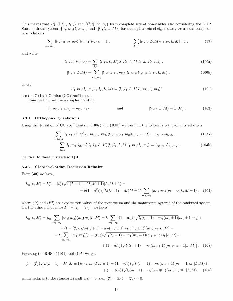
This means that l21, l22, l1,z, l2,z and l21, l22, L2, Lz form complete sets of observables also considering the GUP.Since both the systems |l1,m1; l2,m2〉 and |l1, l2, L,M〉 form complete sets of eigenstates, we use the complete-ness relations ∑

m1,m2

|l1,m1; l2,m2〉〈l1,m1; l2,m2| =1 ,∑M,L

|l1, l2, L,M〉〈l1, l2, L,M | =1 , (99)

and write

|l1,m1; l2,m2〉 =∑M,L

|l1, l2, L,M〉〈l1, l2, L,M |l1,m1; l2,m2〉 , (100a)

|l1, l2, L,M〉 =∑

m1,m2

|l1,m1; l2,m2〉〈l1,m1; l2,m2|l1, l2, L,M〉 , (100b)

where〈l1,m1; l2,m2|l1, l2, L,M〉 = 〈l1, l2, L,M |l1,m1; l2,m2〉∗ (101)

are the Clebsch-Gordan (CG) coefficients.From here on, we use a simpler notation

|l1,m1; l2,m2〉 ≡|m1;m2〉 , and |l1, l2, L,M〉 ≡|L,M〉 . (102)

6.3.1 Orthogonality relations

Using the definition of CG coefficients in (100a) and (100b) we can find the following orthogonality relations∑m1,m2

〈l1, l2, L′,M ′|l1,m1; l2,m2〉〈l1,m1; l2,m2|l1, l2, L,M〉 = δM ′,MδL′,L , (103a)

∑M,L

〈l1,m′1; l2,m′2|l1, l2, L,M〉〈l1, l2, L,M |l1,m1; l2,m2〉 = δm′

1,m1δm′

2,m2, (103b)

identical to those in standard QM.

6.3.2 Clebsch-Gordan Recursion Relation

From (30) we have,

L±|L,M〉 = ~(1− 〈C〉)√L(L+ 1)−M(M ± 1)|L,M ± 1〉 =

= ~(1− 〈C〉)√L(L+ 1)−M(M ± 1)

∑m1,m2

|m1;m2〉〈m1;m2|L,M ± 1〉 , (104)

where 〈P 〉 and 〈P 2〉 are expectation values of the momentum and the momentum squared of the combined system.On the other hand, since L± = l1,± + l2,±, we have

L±|L,M〉 = L±∑

m1,m2

|m1;m2〉〈m1;m2|L,M〉 = ~∑

m1,m2

[(1− 〈C1〉)√l1(l1 + 1)−m1(m1 ± 1)|m1 ± 1;m2〉+

+ (1− 〈C2〉)√l2(l2 + 1)−m2(m2 ± 1)|m1;m2 ± 1〉]〈m1;m2|L,M〉 =

= ~∑

m1,m2

|m1,m2〉[(1− 〈C1〉)√l1(l1 + 1)−m1(m1 ∓ 1)〈m1 ∓ 1;m2|L,M〉+

+ (1− 〈C2〉)√l2(l2 + 1)−m2(m2 ∓ 1)〈m1;m2 ∓ 1|L,M〉] . (105)

Equating the RHS of (104) and (105) we get

(1− 〈C〉)√L(L+ 1)−M(M ± 1)〈m1;m2|LM ± 1〉 = (1− 〈C1〉)

√l1(l1 + 1)−m1(m1 ∓ 1)〈m1 ∓ 1;m2|L,M〉+

+ (1− 〈C2〉)√l2(l2 + 1)−m2(m2 ∓ 1)〈m1;m2 ∓ 1|L,M〉 , (106)

which reduces to the standard result if α = 0, i.e., 〈C〉 = 〈C1〉 = 〈C2〉 = 0.

13

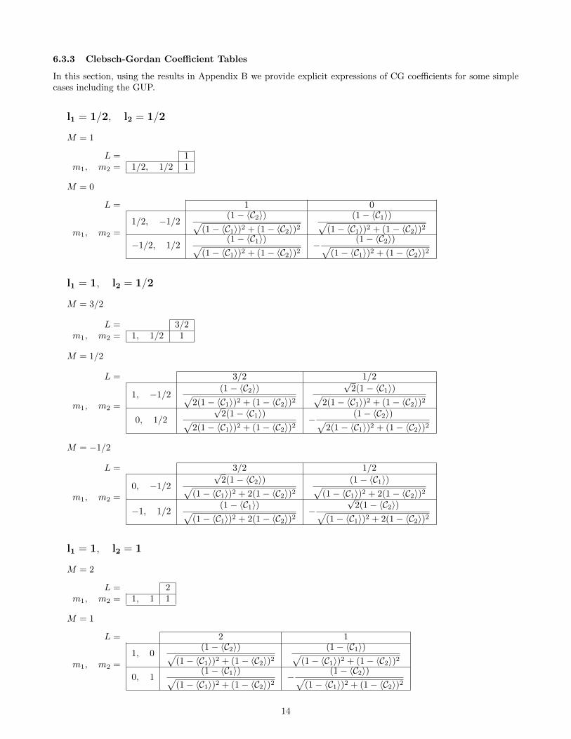
6.3.3 Clebsch-Gordan Coefficient Tables

In this section, using the results in Appendix B we provide explicit expressions of CG coefficients for some simplecases including the GUP.

l1 = 1/2, l2 = 1/2

M = 1

L = 1m1, m2 = 1/2, 1/2 1

M = 0

L = 1 0

m1, m2 =1/2, −1/2

(1− 〈C2〉)√(1− 〈C1〉)2 + (1− 〈C2〉)2

(1− 〈C1〉)√(1− 〈C1〉)2 + (1− 〈C2〉)2

−1/2, 1/2(1− 〈C1〉)√

(1− 〈C1〉)2 + (1− 〈C2〉)2− (1− 〈C2〉)√

(1− 〈C1〉)2 + (1− 〈C2〉)2

l1 = 1, l2 = 1/2

M = 3/2

L = 3/2m1, m2 = 1, 1/2 1

M = 1/2

L = 3/2 1/2

m1, m2 =1, −1/2

(1− 〈C2〉)√2(1− 〈C1〉)2 + (1− 〈C2〉)2

√2(1− 〈C1〉)√

2(1− 〈C1〉)2 + (1− 〈C2〉)2

0, 1/2

√2(1− 〈C1〉)√

2(1− 〈C1〉)2 + (1− 〈C2〉)2− (1− 〈C2〉)√

2(1− 〈C1〉)2 + (1− 〈C2〉)2

M = −1/2

L = 3/2 1/2

m1, m2 =0, −1/2

√2(1− 〈C2〉)√

(1− 〈C1〉)2 + 2(1− 〈C2〉)2(1− 〈C1〉)√

(1− 〈C1〉)2 + 2(1− 〈C2〉)2

−1, 1/2(1− 〈C1〉)√

(1− 〈C1〉)2 + 2(1− 〈C2〉)2−

√2(1− 〈C2〉)√

(1− 〈C1〉)2 + 2(1− 〈C2〉)2

l1 = 1, l2 = 1

M = 2

L = 2m1, m2 = 1, 1 1

M = 1

L = 2 1

m1, m2 =1, 0

(1− 〈C2〉)√(1− 〈C1〉)2 + (1− 〈C2〉)2

(1− 〈C1〉)√(1− 〈C1〉)2 + (1− 〈C2〉)2

0, 1(1− 〈C1〉)√

(1− 〈C1〉)2 + (1− 〈C2〉)2− (1− 〈C2〉)√

(1− 〈C1〉)2 + (1− 〈C2〉)2

14

M = 0

L = 2

m1, m2 =

1, −1(1− 〈C2〉)2√

[(1− 〈C1〉)2 + (1− 〈C2〉)2]2 + 2(1− 〈C1〉)2(1− 〈C2〉)2

0, 02(1− 〈C1〉)(1− 〈C2〉)√

[(1− 〈C1〉)2 + (1− 〈C2〉)2]2 + 2(1− 〈C1〉)2(1− 〈C2〉)2

−1, 1(1− 〈C1〉)2√

[(1− 〈C1〉)2 + (1− 〈C2〉)2]2 + 2(1− 〈C1〉)2(1− 〈C2〉)2

L = 1

m1, m2 =

1, −1(1− 〈C1〉)(1− 〈C2〉)√

(1− 〈C1〉)4 + (1− 〈C2〉)4

0, 0(1− 〈C1〉)2 − (1− 〈C2〉)2√(1− 〈C1〉)4 + (1− 〈C2〉)4

−1, 1 − (1− 〈C1〉)(1− 〈C2〉)√(1− 〈C1〉)4 + (1− 〈C2〉)4

L = 0

m1, m2 =

1, −12(1− 〈C1〉)(1− 〈C2〉)√

[(1− 〈C1〉)2 + (1− 〈C2〈)2]2 + 8(1− 〈C1〉)(1− 〈C2〉)

0, 0 − (1− 〈C1〉)2 + (1− 〈C2〉)2√[(1− 〈C1〉)2 + (1− 〈C2〉)2]2 + 8(1− 〈C1〉)(1− 〈C2〉)

−1, 12(1− 〈C1〉)(1− 〈C2〉)√

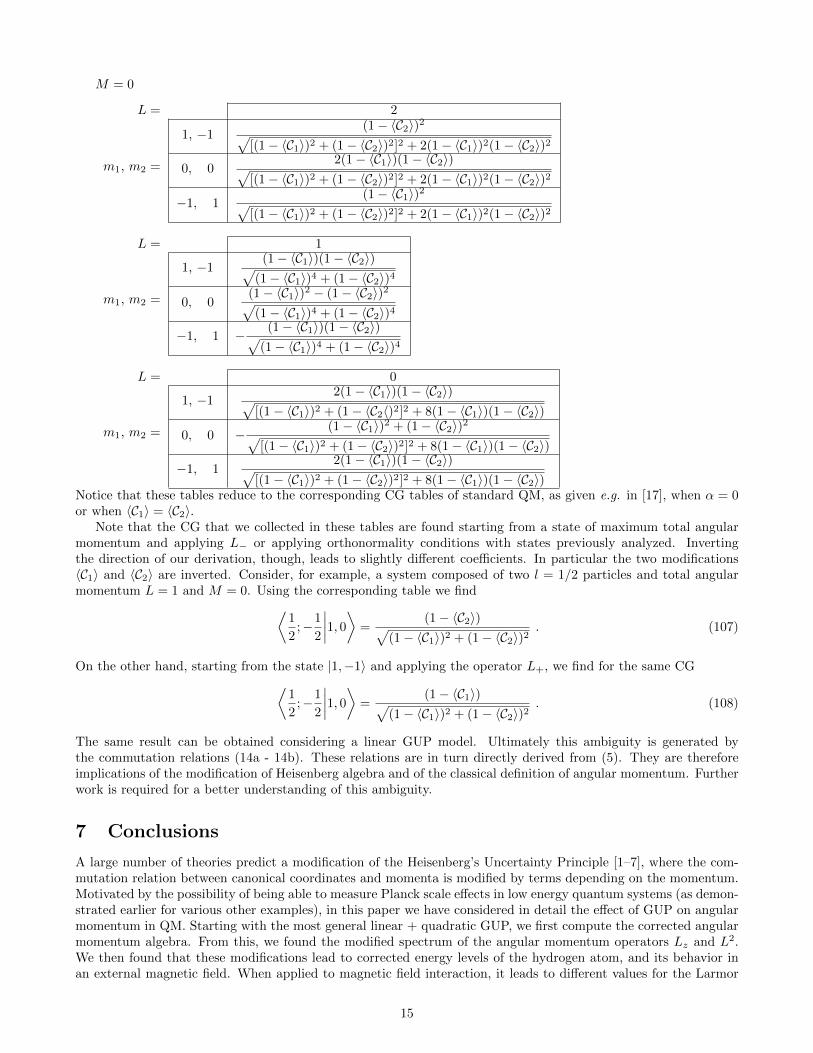
[(1− 〈C1〉)2 + (1− 〈C2〉)2]2 + 8(1− 〈C1〉)(1− 〈C2〉)Notice that these tables reduce to the corresponding CG tables of standard QM, as given e.g. in [17], when α = 0or when 〈C1〉 = 〈C2〉.

Note that the CG that we collected in these tables are found starting from a state of maximum total angularmomentum and applying L− or applying orthonormality conditions with states previously analyzed. Invertingthe direction of our derivation, though, leads to slightly different coefficients. In particular the two modifications〈C1〉 and 〈C2〉 are inverted. Consider, for example, a system composed of two l = 1/2 particles and total angularmomentum L = 1 and M = 0. Using the corresponding table we find⟨

1

2;−1

2

∣∣∣∣1, 0⟩ =(1− 〈C2〉)√

(1− 〈C1〉)2 + (1− 〈C2〉)2. (107)

On the other hand, starting from the state |1,−1〉 and applying the operator L+, we find for the same CG⟨1

2;−1

2

∣∣∣∣1, 0⟩ =(1− 〈C1〉)√

(1− 〈C1〉)2 + (1− 〈C2〉)2. (108)

The same result can be obtained considering a linear GUP model. Ultimately this ambiguity is generated bythe commutation relations (14a - 14b). These relations are in turn directly derived from (5). They are thereforeimplications of the modification of Heisenberg algebra and of the classical definition of angular momentum. Furtherwork is required for a better understanding of this ambiguity.

7 Conclusions

A large number of theories predict a modification of the Heisenberg’s Uncertainty Principle [1–7], where the com-mutation relation between canonical coordinates and momenta is modified by terms depending on the momentum.Motivated by the possibility of being able to measure Planck scale effects in low energy quantum systems (as demon-strated earlier for various other examples), in this paper we have considered in detail the effect of GUP on angularmomentum in QM. Starting with the most general linear + quadratic GUP, we first compute the corrected angularmomentum algebra. From this, we found the modified spectrum of the angular momentum operators Lz and L2.We then found that these modifications lead to corrected energy levels of the hydrogen atom, and its behavior inan external magnetic field. When applied to magnetic field interaction, it leads to different values for the Larmor

15

frequency and for the splitting in the Stern-Gerlach experiment. We finally showed how the modified algebra of thetotal angular momentum of a multi-particle system depends on the number of components and interesting Planckscale modifications to the CG coefficients. It is worth noting that all the modifications derived in this paper arepotentially observable allowing new tests on quantum gravity phenomenology.

It is worthwhile to note that in this paper we compute GUP corrections of the angular momentum spectrumand applied it to the appropriate Schrodinger equation governing non-relativistic systems, such as the hydrogenatom and the Stern-Gerlach experiment. While the corrections to the spectrum will equally apply to relativisticsystems (such as relativistic hydrogen atom), to compute GUP corrections to energy eigenvalues and eigenvectors,the emission spectra etc., one would have to use Dirac equation.

Comparing the results of the present paper, we can obtain upper bounds for the GUP parameter α0. Forinstance, if one assumes that the energy levels of the relativistic hydrogen atom are modified by terms proportionalto α2

0〈p20〉/M2Plc

2 (similar to (45) for the non-relativistic case), deviations from the standard frequency of the 2S - 1Stransition of the order ∼ α2

010−35 Hz are expected. Comparing this with the result in [21], we see that α0 . 1018.This further motivates a study of GUP for the relativistic hydrogen atom, in which the relativistic corrections shouldimpose a much tighter bound on α0. Similarly, for the Stern-Gerlach experiment, one can obtain an estimation ofthe parameter α0 directly comparing the relative error in the splitting δz of an experiment with (70). For example,for a relative error of 10%, one obtains α0 . 1014. Notice that more accurate experiments would result in morestringent bounds.

There remain issues to be better understood, e.g. the dependence of the angular momentum algebra on linearmomentum, and some ambiguity in the CG coefficients. Furthermore, we replaced the operator representing theGUP modification in some formulae by its expectation value. While this suffice to estimate Planck scale effects,in the future we would like to study this further, to see if additional corrections result by retaining the operatorforms. The results presented here can be applied to look for QG signatures, e.g. in spectroscopic as well asastrophysical observations. Furthermore, assuming that the spin algebra also obeys similar modifications, they canalso be applied to a number of quantum systems interacting with magnetic fields, in atomic and nuclear physics.We hope to address these, as well as extensions of our work to relativistic QM [22], in future publications.

Acknowledgments

The authors thank E. C. Vagenas for discussions, and the Referees for useful comments. This work was supportedin part by the Natural Sciences and Engineering Research Council of Canada.

A GUP modified angular momentum commutator

Consider the commutator between two components of the angular momentum

[Li, Lj ] = εimnεjrs[qmpn, qrps] = εimnεirsqm[pn, qr]ps + qr[qm, ps]pn , (109)

Using the GUP commutator in (1), we obtain

[Li, Lj ] = i~εimnεirs

qrpn

[δms − α

(δmsp+

pmpsp

)+ α2(δmsp

2 + 3pmps)

]+

−qmps[δnr − α

(δnrp+

pnprp

)+ α2(δnrp

2 + 3pnpr)

]=

= i~(εmniεmjrqrpn − εnimεnsjqmps)(1− αp+ α2p2) =

= i~[(δirδnj − δnrδij)qrpn − (δisδmj − δijδms)qmps](1− αp+ α2p2) = i~εijkLk(1− αp+ α2p2) , (110)

Consider now

[Li, pl] = εijk(qjpkpl − plqjpk) = i~εijk[δjlpk − α

(δjlppk +

pjplpkp

)+ α2(δjlp

2pk + 3pjplpk)

], (111)

where we used the model in (1). We then have

[Li, p2] = pl[Li, pl] + [Li, pl]pl = 0 . (112)

16

To find the commutation relation between a component of the angular momentum and the magnitude of thelinear momentum, we will first suppose that such a commutator depends only on the vector p

[Li, p] = f(p) . (113)

In this way, using the result just found we have

0 = [Li, p2] = p[Li, p] + [Li, p]p = 2p[Li, p] , (114)

that means, for p 6= 0,[Li, p] = 0 . (115)

Finally we find

[L2, Lj ] = Li[Li, Lj ] + [Li, Lj ]Li = i~εijk[LiLk(1− αp+ α2p2) + Lk(1− αp+ α2p2)Li] =

= i~εijk(LiLk + LkLi)(1− αp+ α2p2) = 0 . (116)

B Clebsch-Gordan Coefficients

In this section, we will calculate several CG coefficients for different values of the total azimuthal and magneticquantum numbers, L and M, referring these values to the maximum values Lmax = l1 + l2 and Mmax = Lmax, wherel1 and l2 are the azimuthal quantum numbers of the single systems.

B.1 L = Lmax, M = Lmax

For this case, the state represented by the total angular momentum can be related to just one of the states concerningthe individual angular momenta, that is

|Lmax, Lmax〉 = |l1; l2〉 . (117)

This means that the CG coefficient for this case is simply

〈l1; l2|Lmax, Lmax〉 = 1 . (118)

B.2 M = Lmax − 1

Two states are possible

|l1 − 1; l2〉 , |l1; l2 − 1〉 . (119)

B.2.1 L = Lmax

Applying the lowering operator L− = l1,− + l2,− we find

|Lmax, Lmax − 1〉 ∝ L−|Lmax, Lmax〉 = (l1,− + l2,−)|l1; l2〉 =

= ~[(1− 〈C1〉)√

2l1|l1 − 1; l2〉+ (1− 〈C2〉)√

2l2|l1; l2 − 1〉] , (120)

where we used the result in (118) and the relation (30). Since both these coefficients are positive (we are assumingthat 〈C〉 is smaller than 1), the Condon–Shortley phase convention is already fulfilled, we need just to normalizethis combination since

||L−|Lmax, Lmax − 1〉||2 = 2~2[(1− 〈C1〉)2l1 + (1− 〈C2〉)2l2] . (121)

Thus, the two CG coefficient for this case are

〈l1 − 1; l2|Lmax, Lmax − 1〉 =(1− 〈C1〉)

√l1√

(1− 〈C1〉)2l1 + (1− 〈C2〉)2l2, (122a)

〈l1; l2 − 1|Lmax, Lmax − 1〉 =(1− 〈C2〉)

√l2√

(1− 〈C1〉)2l1 + (1− 〈C2〉)2l2. (122b)

17

B.2.2 L = Lmax − 1

In this case, we will find the two CG coefficients for |Lmax − 1, Lmax − 1〉 applying the orthonormality conditionbetween this state and |Lmax, Lmax− 1〉. The state in this case can be written as a linear combination of |l1− 1; l2〉and |l1; l2 − 1〉

|Lmax − 1, Lmax − 1〉 = G10|l1 − 1; l2〉+G01|l1; l2 − 1〉 . (123)

From the orthogonality condition we find

〈Lmax, Lmax−1|Lmax−1, Lmax−1〉 =(1− 〈C1〉)

√l1√

(1− 〈C1〉)2l1 + (1− 〈C2〉)2l2G10 +

(1− 〈C2〉)√l2√

(1− 〈C1〉)2l1 + (1− 〈C2〉)2l2G01 = 0 ,

(124)obtaining

G01 = − (1− 〈C1〉)√l1

(1− 〈C2〉)√l2G10 . (125)

Normalizing the state

|G10|2[1 +

(1− 〈C1〉)2l1(1− 〈C2〉)2l2

]= |G10|2

(1− 〈C1〉)2l1 + (1− 〈C2〉)2l2(1− 〈C2〉)2l2

= 1 , (126)

and imposing the Condon–Shortley phase convention

〈l1;Lmax − 1− l1|Lmax − 1, Lmax − 1〉 = 〈l1; l2 − 1|Lmax − 1, Lmax − 1〉 ≥ 0 , (127)

we have

〈l1 − 1; l2|Lmax − 1, Lmax − 1〉 = − (1− 〈C2〉)√l2√

(1− 〈C1〉)2l1 + (1− 〈C2〉)2l2, (128a)

〈l1; l2 − 1|Lmax − 1, Lmax − 1〉 =(1− 〈C1〉)

√l1√

(1− 〈C1〉)2l1 + (1− 〈C2〉)2l2. (128b)

B.3 M = Lmax − 2

In this case the three possible states are

|l1, l1 − 2; l2, l2〉 , |l1, l1 − 1; l2, l2 − 1〉 , |l1, l1; l2, l2 − 2〉 . (129)

B.3.1 L = Lmax

The CG coefficients for this case are found acting one time with L− on the state |Lmax, Lmax − 1〉

L−|Lmax, Lmax − 2〉 ∝ (l1,− + l2,−)[〈l1 − 1; l2|Lmax, Lmax − 1〉|l1 − 1; l2〉+ 〈l1; l2 − 1|Lmax, Lmax − 1〉|l1; l2 − 1〉] =

= ~〈l1 − 1; l2|Lmax, Lmax − 1〉[(1− 〈C1〉)√

4l1 − 2|l1 − 2; l2〉+ (1− 〈C2〉)√

2l2|l1 − 1; l2 − 1〉]+

+ 〈l1; l2 − 1|Lmax, Lmax − 1〉[(1− 〈C1〉)√

2l1|l1 − 1; l2 − 1〉+ (1− 〈C2〉)√

4l2 − 2|l1; l2 − 2〉] =

= ~

√2(1− 〈C1〉)2

√l1(2l1 − 1)√

(1− 〈C1〉)2l1 + (1− 〈C2〉)2l2|l1 − 2; l2〉+

2√

2(1− 〈C1〉)(1− 〈C2〉)√l1l2√

(1− 〈C1〉)2l1 + (1− 〈C2〉)2l2|l1 − 1; l2 − 1〉+

+

√2(1− 〈C2〉)2

√l2(2l2 − 1)√

(1− 〈C2〉)2l2 + (1− 〈C1〉)2l1|l1; l2 − 2〉

, (130)

where we used the relation (30) and the coefficients in (122). Normalizing this last result we find

〈l1 − 2; l2|Lmax, Lmax − 2〉 =(1− 〈C1〉)2

√l1(2l1 − 1)

Ω0, (131a)

〈l1 − 1; l2 − 1|Lmax, Lmax − 2〉 =2(1− 〈C1〉)(1− 〈C2〉)

√l1l2

Ω0, (131b)

〈l1; l2 − 2|Lmax, Lmax − 2〉 =(1− 〈C2〉)2

√l2(2l2 − 1)

Ω0, (131c)

18

whereΩ0 =

√(1− 〈C1〉)4l1(2l1 − 1) + 4(1− 〈C1〉)2(1− 〈C2〉)2l1l2 + (1− 〈C2〉)4l2(2l2 − 1) . (132)

Since these coefficients are all positive, the phase convention is already fulfilled.

B.3.2 L = Lmax − 1

To find the CG coefficients for this case we apply L− on the state |Lmax − 1, Lmax − 1〉

L−|Lmax − 1, Lmax − 1〉 =

= (l1,− + l2,−)[〈l1 − 1; l2|Lmax − 1, Lmax − 1〉|l1 − 1; l2〉+ 〈l1; l2 − 1|Lmax − 1, Lmax − 1〉|l1; l2 − 1〉] =

= ~〈l1 − 1; l2|Lmax − 1, Lmax − 1〉[(1− 〈C1〉)√

4l1 − 2|l1 − 2; l2〉+ (1− 〈C2〉)√

2l2|l1 − 1; l2 − 1〉]+

+ ~〈l1; l2 − 1|Lmax − 1, Lmax − 1〉[(1− 〈C1〉)√

2l1|l1 − 1; l2 − 1〉+ (1− 〈C2〉)√

4l2 − 2|l1; l2 − 2〉] ∝

∝ −~(1− 〈C1〉)(1− 〈C2〉)√

4l1 − 2√l2|l1 − 2; l2〉+ ~[(1− 〈C1〉)2

√2l1 − (1− 〈C2〉)2

√2l2]|l1 − 1; l2 − 1〉+

+ ~(1− 〈C1〉)(1− 〈C2〉)√l1√

4l2 − 2|l1 − 1; l2 − 2〉 . (133)

Normalizing and using the Condon-Shortley convention we thus find

〈l1 − 2; l2|Lmax − 1, Lmax − 2〉 =(1− 〈C1〉)(1− 〈C2〉)

√4l1 − 2

√l2

Ω1, (134a)

〈l1 − 1; l2 − 1|Lmax − 1, Lmax − 2〉 = − (1− 〈C1〉)2√

2l1 − (1− 〈C2〉)2√

2l2Ω1

, (134b)

〈l1; l2 − 2|Lmax − 1, Lmax − 2〉 = − (1− 〈C1〉)(1− 〈C2〉)√l1√

4l2 − 2

Ω1, (134c)

with

Ω1 =√

2(1− 〈C1〉)4l21 + 2(1− 〈C1〉)2(1− 〈C2〉)2(2l1l2 − l1 − l2) + 2(1− 〈C2〉)4l22 . (135)

B.3.3 L = Lmax − 2

As first step, let us define the CG coefficients for this case in the following way

|Lmax − 2, Lmax − 2〉 = G20|l1 − 2, l2〉+G11|l1 − 1, l2 − 1〉+G02|l1, l2 − 2〉 . (136)

Considering the orthogonality between the states |Lmax − 2, Lmax − 2〉 and |Lmax − 1, Lmax − 2〉

−G20(1− 〈C1〉)(1− 〈C2〉)√

4l1 − 2√l2 +G11[(1− 〈C1〉)2

√2l1 − (1− 〈C2〉)2

√2l2]+

+G02(1− 〈C1〉)(1− 〈C2〉)√l1√

4l2 − 2 = 0 , (137)

and the orthogonality between the first state and |Lmax, Lmax − 2〉

G20(1− 〈C1〉)2√l1(2l1 − 1) + 2G11(1− 〈C1〉)(1− 〈C2〉)

√l1l2 +G02(1− 〈C2〉)2

√l2(2l2 − 1) = 0 , (138)

whence

G11 = −G201− 〈C1〉1− 〈C2〉

√2l1 − 1

2√l2−G02

1− 〈C2〉1− 〈C1〉

√2l2 − 1

2√l1

. (139)

Inserting this last result in (137) we find

−G201− 〈C1〉1− 〈C2〉

√2l1 − 1√

2l2

[(1− 〈C2〉)2l2 + (1− 〈C1〉)2l1

]+

+G021− 〈C2〉1− 〈C1〉

√2l2 − 1√

2l1

[(1− 〈C1〉)2l1 + (1− 〈C2〉)2l2

]= 0⇒

⇒ G20 = G02

√l2(2l2 − 1)√l1(2l1 − 1)

, (140)

19

whence, using this result in (139) we obtain

G11 = −G02

√2l2 − 1

2√l1

(1− 〈C1〉)2 + (1− 〈C2〉)2

(1− 〈C1〉)(1− 〈C2〉). (141)

Imposing the normalization condition

|G02|2l2(2l2 − 1)

l1(2l1 − 1)+ |G02|2

2l2 − 1

4l1

(1− 〈C1〉)4 + (1− 〈C2〉)4 + 2(1− 〈C1〉)2(1− 〈C2〉)2

(1− 〈C1〉)2(1− 〈C2〉)2+ |G02|2 = 1 (142)

and the Condon-Shortley phase convention we have

〈l1; l2 − 2|Lmax − 2, Lmax − 2〉 =2√l2(2l2 − 1)(1− 〈C1〉)(1− 〈C2〉)

Ω2, (143a)

〈l1; l2 − 2|Lmax − 2, Lmax − 2〉 =−√

(2l1 − 1)(2l2 − 1)[(1− 〈C1〉)2 + (1− 〈C2〉)2]

Ω2, (143b)

〈l1; l2 − 2|Lmax − 2, Lmax − 2〉 =2√l1(2l1 − 1)(1− 〈C1〉)(1− 〈C2〉)

Ω2, (143c)

where

Ω2 = 2(1− 〈C1〉)2(1− 〈C2〉)2[2l2(2l2 − 1) + 2l1(2l1 − 1) + (2l1 − 1)(2l2 − 1)]+

+ (2l1 − 1)(2l2 − 1)[(1− 〈C1〉)4 + (1− 〈C2〉)4]1/2 . (144)

References

[1] D. Amati, M. Ciafaloni, and G. Veneziano, “Can spacetime be probed below the string size?”, Physics LettersB, vol. 216, no. 1, pp. 41–47, 1989.

[2] G. Amelino-Camelia, “Doubly-Special Relativity: First Results and Key Open Problems”, International Jour-nal of Modern Physics D, vol. 11, no. 10, pp. 1643–1669, 2002.

[3] L. J. Garay, “Quantum Gravity and Minimum Length”, International Journal of Modern Physics A, vol. 10,no. 02, pp. 145–165, 1995.

[4] D. Gross and P. Mende, “String theory beyond the Planck scale”, Nuclear Physics B, vol. 303, pp. 407–454,jul 1988.

[5] M. Maggiore, “A generalized uncertainty principle in quantum gravity.”, Physics Letter B, vol. 304, pp. 65–69,1993.

[6] M. Maggiore, “The algebraic structure of the generalized uncertainty principle.”, Physics Letter B, vol. 319,pp. 83–86, 1993.

[7] F. Scardigli, “Generalized uncertainty principle in quantum gravity from micro-black hole gedanken experi-ment”, Physics Letters B, vol. 452, no. 1–2, pp. 39–44, 1999.

[8] S. Das and E. C. Vagenas, “Phenomenological implications of the generalized uncertainty principle”, CanadianJournal of Physics, vol. 87, no. 3, pp. 233–240, 2009.

[9] A. F. Ali, S. Das, and E. C. Vagenas, “A proposal for testing quantum gravity in the lab”, Phys. Rev. D,vol. 84, p. 44013, aug 2011.

[10] A. F. Ali, S. Das, and E. C. Vagenas, “Discreteness of space from the generalized uncertainty principle.”,Physics Letters B, vol. 678, no. 5, pp. 497–499, 2009.

[11] I. Pikovski, M. R. Vanner, M. Aspelmeyer, M. S. Kim, and C. Brukner, “Probing Planck-scale physics withquantum optics”, Nature Physics, vol. 8, pp. 393–397, 2012.

[12] A. Kempf, G. Mangano, and R. B. Mann, “Hilbert space representation of the minimal length uncertaintyrelation.”, Physical Review D, vol. 52, pp. 1108–1118, 1995.

20

[13] S. Pramanik and S. GhoshH, “GUP-based and Snyder noncommutative algebras, relativistic particle models,deformed symmetries and interaction: a unified approach”, International Journal of Modern Physics A, vol. 28,no. 27, p. 1350131, 2013.

[14] S. Das, E. C. Vagenas, and A. F. Ali, “Discreteness of space from GUP II: Relativistic wave equations”,Physics Letters B, vol. 690, no. 4, pp. 407–412, 2010.

[15] S. Deb, S. Das, and E. C. Vagenas, “Discreteness of space from GUP in a weak gravitational field”, PhysicsLetters B, vol. 755, pp. 17–23, 2016.

[16] A. Messiah, Quantum Mechanics. Dover books on physics, Dover Publications, 1961.

[17] A. Goswami, Quantum mechanics. Wm. C. Brown, 1992.

[18] J. L. Basdevant and J. Dalibard, Quantum Mechanics. Advanced Texts in Physics, Springer Berlin Heidelberg,2002.

[19] B. Friedrich and D. Herschbach, “Stern and Gerlach: How a bad cigar helped reorient atomic physics”, PhysicsToday, vol. 56, no. 12, p. 53, 2003.

[20] S. Pramanik, S. Ghosh, and P. Pal, “Conformal invariance in noncommutative geometry and mutually inter-acting Snyder particles”, Phys. Rev. D, vol. 90, p. 105027, nov 2014.

[21] A. Matweev et al., “Precision Measurement of the Hydrogen 1 S-2 S Frequency via a 920-km Fiber Link”,Physical Review Letters, vol. 110, no. 23, 2013.

[22] P. Bosso and S. Das, In Preparation,

21