the wageningen lowland runoff simulator (walrus… · the wageningen lowland runoff simulator...

Geosci. Model Dev., 7, 2313–2332, 2014www.geosci-model-dev.net/7/2313/2014/doi:10.5194/gmd-7-2313-2014© Author(s) 2014. CC Attribution 3.0 License.

The Wageningen Lowland Runoff Simulator (WALRUS): a lumpedrainfall–runoff model for catchments with shallow groundwaterC. C. Brauer, A. J. Teuling, P. J. J. F. Torfs, and R. Uijlenhoet

Hydrology and Quantitative Water Management Group, Wageningen University, Wageningen, the Netherlands

Correspondence to:C. C. Brauer ([email protected])

Received: 2 January 2014 – Published in Geosci. Model Dev. Discuss.: 12 February 2014Revised: 30 June 2014 – Accepted: 23 July 2014 – Published: 10 October 2014

Abstract. We present the Wageningen Lowland Runoff Sim-ulator (WALRUS), a novel rainfall–runoff model to fill thegap between complex, spatially distributed models whichare often used in lowland catchments and simple, para-metric (conceptual) models which have mostly been devel-oped for sloping catchments. WALRUS explicitly accountsfor processes that are important in lowland areas, notably(1) groundwater–unsaturated zone coupling, (2) wetness-dependent flow routes, (3) groundwater–surface water feed-backs and (4) seepage and surface water supply. WALRUSconsists of a coupled groundwater–vadose zone reservoir, aquickflow reservoir and a surface water reservoir. WALRUSis suitable for operational use because it is computationallyefficient and numerically stable (achieved with a flexible timestep approach). In the open source model code default rela-tions have been implemented, leaving only four parameterswhich require calibration. For research purposes, these de-faults can easily be changed. Numerical experiments showthat the implemented feedbacks have the desired effect onthe system variables.

1 Introduction

Lowlands, especially those in river deltas, are often denselypopulated and centres of agricultural production, economicactivity and transportation. Therefore, socio-economic con-sequences of natural hazards are specially large in these ar-eas. In addition, their low elevations and mild slopes increasetheir vulnerability to flooding (coastal, fluvial and pluvial),climate change, and deterioration of water quality. To mit-igate natural and human disasters, hydrological models canbe used by water managers as a tool for risk assessment andinfrastructure design. Lowlands, defined here as areas with

shallow groundwater tables, exist all over the world: 13 %of the world’s land surface has groundwater tables shallowerthan 2 m and 22 % shallower than 4 m (Fig.1; data fromFanet al., 2013). This indicates that being able to understand andmodel lowland-specific hydrologic processes is beneficial forscientists and practitioners around the world.

Many types of hydrological models exist and they varywidely in their degree of complexity. The appropriatedegree of complexity depends on the objectives of themodel study and the catchment the model is applied to(Wagener et al., 2001). Here, we focus on models to simu-late catchment runoff, or, more accurately, the changes inriver discharge resulting from hydrological processes withinthe catchment (the terms runoff and discharge are used in-terchangeably in this paper). Between detailed, spatially dis-tributed models and black box models lies the class of para-metric rainfall–runoff models, which simplify hydrologicalsystems into a collection of reservoirs and flow routes, cap-turing the essence of the hydrological processes, while re-stricting the number of parameters (Wagener and Wheater,2004). Widely used examples of parametric rainfall–runoffmodels are the Tank model (Sugawara et al., 1974), PDM(Moore, 1985), HBV (Bergström and Forsman, 1973), theSacramento model (Burnash, 1995), ARNO (Todini, 1996),SWAT (Arnold et al., 1998) and GR4J (Edijatno et al., 1999;Perrin et al., 2003). However, these models have all been de-veloped for sloping catchments and errors may arise whenapplied to lowland catchments, because essential processes(e.g. capillary rise) are not accounted for and typical con-ditions (e.g. influence of surface water on groundwater) arenot met. Examples of the resulting problems are presentedby Bormann and Elfert(2010), who used WaSiM-ETH(Schulla and Jasper, 2007) andKoch et al.(2013), who usedSWAT, both in northeastern Germany.

Published by Copernicus Publications on behalf of the European Geosciences Union.

2314 C. C. Brauer et al.: WALRUS: a lumped rainfall–runoff model for catchments with shallow groundwater

Groundwaterdepth [m]0−22−4>4

Figure 1. Locations with shallow groundwater (based on data fromFan et al., 2013). Lowland areas can be found all over the worldand often in densely populated areas, which shows the relevance ofWALRUS for application outside the Netherlands.

For realistic simulations of runoff, the model structureshould represent the main catchment processes and there-fore several models have been developed for specific catch-ment and climate types: (Dynamic) TOPMODEL (Beven andKirkby, 1979; Beven and Freer, 2001) for sloping catch-ments, VIC (Liang et al., 1996) for areas prone to saturationexcess overland flow and LGSI (Van der Velde et al., 2009)for data-rich lowland catchments. In addition, flexible modelframeworks, e.g. (SUPER)FLEX (Fenicia et al., 2006, 2011)and FUSE (Clark et al., 2008), have been developed to al-low for adaptation of the model structure to individual catch-ments.

A parametric rainfall–runoff model for lowland catch-ments, the Wageningen model, was developed at the Hy-drology and Quantitative Water Management Group of Wa-geningen University in the 1970s (Stricker and Warmerdam,1982). This parametric model accounts for certain lowland-specific processes: capillary rise and a dynamic division be-tween fast and slow flow routes as a function of catchmentwetness. However, other lowland-specific processes are notincluded in the Wageningen model: the saturated and unsat-urated zone are disconnected and no feedbacks are possiblebetween groundwater and surface water. Although the Wa-geningen model has been widely applied in many catchmentsinside and outside the Netherlands, users have indicated anumber of serious shortcomings, both of numeric and con-ceptual nature.

In response to this demand, we have developed the Wa-geningen Lowland Runoff Simulator (WALRUS). We aimedfor an entirely new model to simulate runoff in lowlandcatchments, which can be used both for multi-year water bal-ance studies and for single rainfall–runoff events. The modelwas designed to have an understandable model structure thatincorporates the most important processes and feedbacks,with fewer than six parameters of which the values do notchange with the temporal resolution at which the model isrun.

In this paper we present WALRUS. First, we describe thethreefold motivation for model development: general chal-lenges in rainfall–runoff modelling (Sect.2), the two con-trasting lowland field sites which were used in the modeldevelopment (Sect.3), and challenges in modelling rainfall–runoff processes in lowland catchments (Sect.4). In Sect.5we explain the model structure in detail. Section6 containsthe implementation of the model (computer code) and Sect.7the conclusions. A detailed model evaluation is discussed ina companion paper (Brauer et al., 2014).

2 Challenges in rainfall–runoff modelling

Water managers in lowland areas often use complex hydro-logical models. MIKE-SHE (Refsgaard and Storm, 1995),HEC-RAS (Brunner, 1995) and SOBEK (Deltares, 2013)have detailed schematisations of surface water networks tosimulate the complex flow routing in intensively drained ar-eas. HYDRUS (Šimunek et al., 2008) and SWAP (Van Damet al., 2008) have detailed vertical schematisations to simu-late unsaturated–saturated zone coupling. Regional ground-water models, such as MODFLOW (McDonald and Har-baugh, 1984), account for seepage and lateral groundwa-ter flow. Combinations of several of these models can beused to account for groundwater–surface water feedbacks,such as SHE (Abbott et al., 1986), HydroGeoSphere (Ther-rien et al., 2006) SIMGRO (Querner, 1988; Van Walsum andVeldhuizen, 2011) or NHI (Prinsen and Becker, 2011).

However, complex models have important disadvantagesand simple models important advantages, particularly con-sidering four aspects. The first aspect concerns overparam-eterisation. Model parameters account for differences in re-sponse times or recession shapes between catchments withthe same dominant processes (represented by the modelstructure). With too many parameters, an inappropriatemodel structure can be compensated for by mathematicallyfitting the model to the calibration data (Kirchner, 2006).An overparameterised model may perform well during cal-ibration, but unsatisfactorily during validation (Perrin et al.,2001) and in different (future) climate regimes (e.g.Seibert,1999).

The second aspect concerns parameter identification. Therisk of parameter dependence and equifinality (where differ-ent combinations of parameter values lead to similar results,Beven and Binley, 1992; Uhlenbrook et al., 1999) increaseswith the number of parameters. With one objective function,only typically three to five parameters can be identified (Jake-man and Hornberger, 1993; Beven, 1989). Multi-objectivecalibration allows more parameters to be calibrated (e.g.Gupta et al., 1998; Efstratiadis and Koutsoyiannis, 2010),but for many catchments only discharge data are available(Soulsby et al., 2008). It is therefore beneficial to be able toidentify the effect of each parameter on the modelled dis-charge time series.

Geosci. Model Dev., 7, 2313–2332, 2014 www.geosci-model-dev.net/7/2313/2014/

C. C. Brauer et al.: WALRUS: a lumped rainfall–runoff model for catchments with shallow groundwater 2315

The third aspect concerns physical representation. A sim-ple, parametric model structure enables users to quicklygrasp the processes covered by each model element andthe influence of each parameter. Values of effective modelparameters cannot be determined with point measurements(Wagener, 2003; Vrugt et al., 2005), but model parametersdo have physical connotations and can be explained quali-tatively from catchment characteristics and field experience(Seibert and McDonnell, 2002). The effect of small-scaleheterogeneity on catchment-scale processes is included im-plicitly in the model parameters (Beven, 1995; Kirchner,2006; McDonnell et al., 2007).

The final aspect concerns practical applicability. Compu-tational efficiency facilitates operational forecasting and dataassimilation (Liu et al., 2012; Rakovec et al., 2012). Ensem-bles can be generated for different forcing data or parame-ter sets to indicate predictive uncertainty (Krzysztofowicz,2001). In addition, more complex and time-consuming algo-rithms can be used for calibration (e.g. DREAM byVrugtet al., 2008) or parameter uncertainty estimation (e.g. GLUEby Beven and Binley, 1992). Avoiding the need to constructa model with channel cross sections and soil layers for eachcatchment can also be advantageous. These four aspects mo-tivated us to develop a parsimonious model and apply Oc-cam’s razor where possible.

3 Experience from two contrasting lowland catchments

Field experience and data from two contrasting field sites inthe Netherlands have been used to develop the model struc-ture. The Hupsel Brook catchment in the east has slightlysloping surfaces and drainage is driven by gravity (freelydraining). The Cabauw polder in the west is flat and its waterlevels are controlled with weirs and supply of surface water.The Hupsel Brook catchment is 6.5 km2, its soils consist of0.2–11 m of loamy sand on an impermeable clay layer andland cover is mostly grass (59 %) and some maize (33 %).The Cabauw polder is 0.5 km2, its soils consist of about70 cm heavy clay on peat and land cover is 80 % grass, 15 %maize and 5 % surface water. A more detailed description ofboth catchments and observations is presented in an accom-panying paper (Brauer et al., 2014).

From the Hupsel Brook catchment, we used combined ob-servations of groundwater and soil moisture (from a neu-tron probe at 12 depths, ranging from 0.15 to 2.05 m; period1976–1984) at six locations, which represent the spatial vari-ability in the catchment well. Potential evapotranspirationwas estimated with the method ofThom and Oliver(1977).During the growing seasons (15 April–14 September) of1976 through 1982 daily sums of actual evapotranspiration(ETact) have been computed with the energy budget method:net radiation was measured and wind and temperature profilemeasurements were used to estimate sensible and groundheat flux. Evapotranspiration was then estimated as residual

of the energy budget (for more information seeStricker andBrutsaert, 1978). In addition, we used data from 1993: dis-charge measured with a type of H-flume, groundwater depthsmeasured at the meteorological station and total phosphorus,nitrate and chloride concentrations measured at the catch-ment outlet.

From the Cabauw polder, we used daily soil moisture datafrom four arrays of six TDR sensors between 5 and 73 cmdeep from the period 2003–2010. Groundwater depth wasmeasured at the same location. Potential evapotranspiration(ETpot) was estimated with the method ofMakkink (1957).Actual evapotranspiration (ETact) was determined with anenergy balance method (Beljaars and Bosveld, 1997). Net ra-diation and ground heat flux were measured and the Bowenratio was determined with eddy covariance measurements.Evapotranspiration was obtained by dividing the availableenergy (net radiation minus ground heat flux) between la-tent and sensible heat fluxes according to the Bowen ratio.Because ETact estimated with this method was on average4 % higher than ETpot during well-watered conditions, wedivided ETact by 1.04.

4 Challenges in modelling rainfall–runoff processesin lowland catchments

In this section we discuss some characteristics which affecthydrological processes in lowland catchments. We discusshow they are represented in some widely used rainfall–runoffmodels and how they are accounted for explicitly in WAL-RUS.

4.1 Groundwater–unsaturated zone coupling

Whereas in most models percolation is assumed to be drivenby downward gravitational forces only, the vertical profile ofmoisture content in lowland soils is influenced by capillaryforces associated with the presence of a shallow groundwatertable. Percolation is slower and evapotranspiration remainshigh in dry periods, because storage deficits are replenishedby capillary rise (e.g.Hopmans and van Immerzeel, 1988;Stenitzer et al., 2007). Therefore, the vadose zone and thegroundwater zone form a tightly coupled system and feed-backs should be included in models for lowland catchments(Chen and Hu, 2004). In addition, when groundwater risesto the soil surface, the unsaturated zone shrinks and its stor-age capacity decreases. It is therefore important to includea dynamic unsaturated zone in the model, which is influencedby the surface fluxes precipitation and evapotranspiration aswell as by the (dynamic) groundwater table below.

Many conceptual rainfall–runoff models, e.g. HBV andthe Sacramento model contain separate reservoirs forsoil moisture and groundwater, allowing only downwardmovement of groundwater without considering feedbacks.One version of PDM does reduce recharge when the soil

www.geosci-model-dev.net/7/2313/2014/ Geosci. Model Dev., 7, 2313–2332, 2014


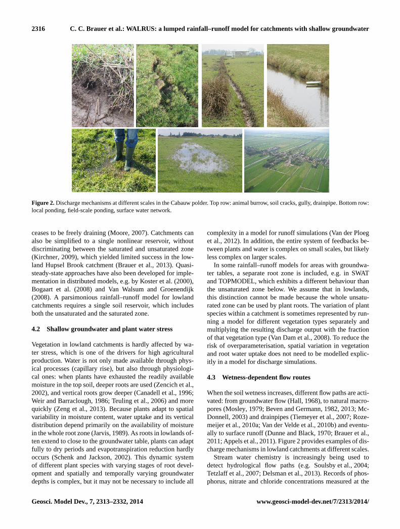
Figure 2.Discharge mechanisms at different scales in the Cabauw polder. Top row: animal burrow, soil cracks, gully, drainpipe. Bottom row:local ponding, field-scale ponding, surface water network.

ceases to be freely draining (Moore, 2007). Catchments canalso be simplified to a single nonlinear reservoir, withoutdiscriminating between the saturated and unsaturated zone(Kirchner, 2009), which yielded limited success in the low-land Hupsel Brook catchment (Brauer et al., 2013). Quasi-steady-state approaches have also been developed for imple-mentation in distributed models, e.g. byKoster et al.(2000),Bogaart et al.(2008) and Van Walsum and Groenendijk(2008). A parsimonious rainfall–runoff model for lowlandcatchments requires a single soil reservoir, which includesboth the unsaturated and the saturated zone.

4.2 Shallow groundwater and plant water stress

Vegetation in lowland catchments is hardly affected by wa-ter stress, which is one of the drivers for high agriculturalproduction. Water is not only made available through phys-ical processes (capillary rise), but also through physiologi-cal ones: when plants have exhausted the readily availablemoisture in the top soil, deeper roots are used (Zencich et al.,2002), and vertical roots grow deeper (Canadell et al., 1996;Weir and Barraclough, 1986; Teuling et al., 2006) and morequickly (Zeng et al., 2013). Because plants adapt to spatialvariability in moisture content, water uptake and its verticaldistribution depend primarily on the availability of moisturein the whole root zone (Jarvis, 1989). As roots in lowlands of-ten extend to close to the groundwater table, plants can adaptfully to dry periods and evapotranspiration reduction hardlyoccurs (Schenk and Jackson, 2002). This dynamic systemof different plant species with varying stages of root devel-opment and spatially and temporally varying groundwaterdepths is complex, but it may not be necessary to include all

complexity in a model for runoff simulations (Van der Ploeget al., 2012). In addition, the entire system of feedbacks be-tween plants and water is complex on small scales, but likelyless complex on larger scales.

In some rainfall–runoff models for areas with groundwa-ter tables, a separate root zone is included, e.g. in SWATand TOPMODEL, which exhibits a different behaviour thanthe unsaturated zone below. We assume that in lowlands,this distinction cannot be made because the whole unsatu-rated zone can be used by plant roots. The variation of plantspecies within a catchment is sometimes represented by run-ning a model for different vegetation types separately andmultiplying the resulting discharge output with the fractionof that vegetation type (Van Dam et al., 2008). To reduce therisk of overparameterisation, spatial variation in vegetationand root water uptake does not need to be modelled explic-itly in a model for discharge simulations.

4.3 Wetness-dependent flow routes

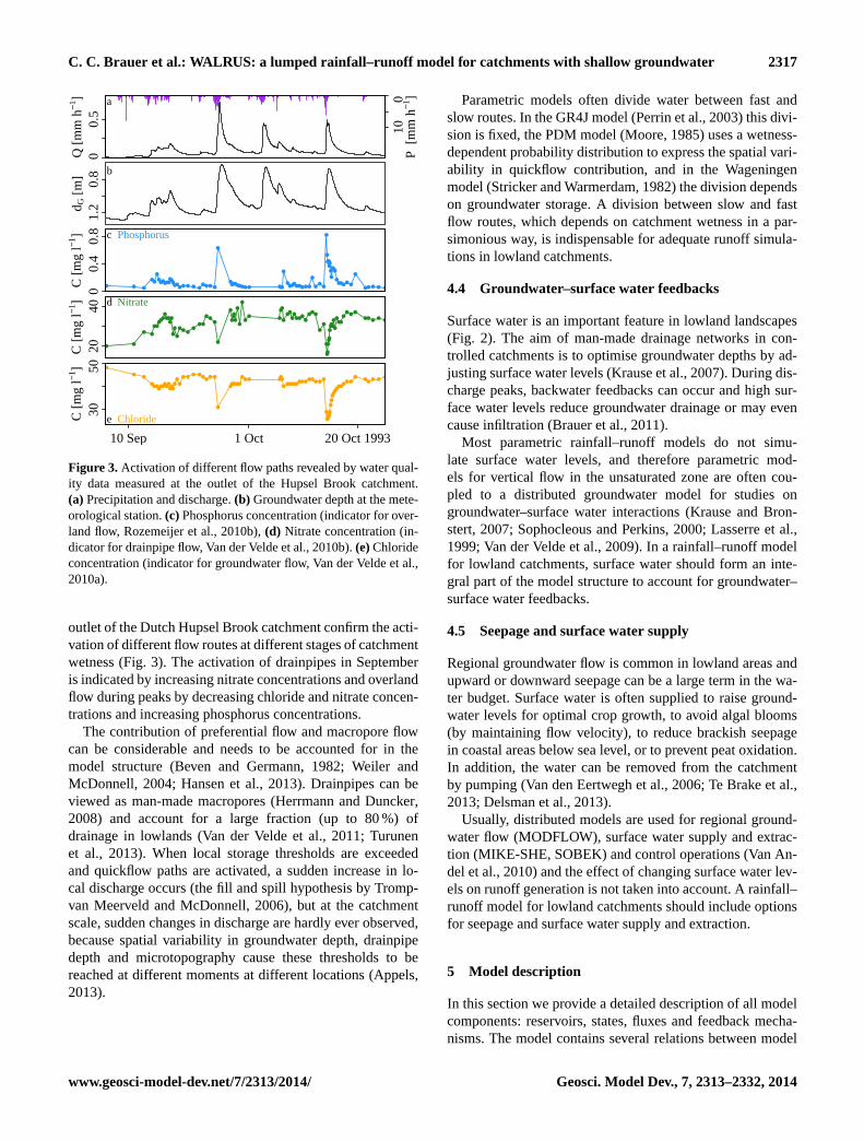
When the soil wetness increases, different flow paths are acti-vated: from groundwater flow (Hall, 1968), to natural macro-pores (Mosley, 1979; Beven and Germann, 1982, 2013; Mc-Donnell, 2003) and drainpipes (Tiemeyer et al., 2007; Roze-meijer et al., 2010a; Van der Velde et al., 2010b) and eventu-ally to surface runoff (Dunne and Black, 1970; Brauer et al.,2011; Appels et al., 2011). Figure2provides examples of dis-charge mechanisms in lowland catchments at different scales.

Stream water chemistry is increasingly being used todetect hydrological flow paths (e.g.Soulsby et al., 2004;Tetzlaff et al., 2007; Delsman et al., 2013). Records of phos-phorus, nitrate and chloride concentrations measured at the


C. C. Brauer et al.: WALRUS: a lumped rainfall–runoff model for catchments with shallow groundwater 2317Q

[mm

h−1

] 0

0.5

100

P

[m

m h−1

]a

d G [m

]1.

20.

8 b

C [m

g l−1

]

● ● ●

●●

●●●●●●●

●●●●●

●●● ● ●●●●●

●

●●●●●●●●●● ●●●

●

●●●●●●●●●

●

●●

●

●

●

●●●●●

●

●

●●●

●●●●●●

●

●●● ● ●

●

● ●

●

00.

40.

8 c Phosphorus

C [m

g l−1

]

● ●

● ●

●●●●

●●●●

●●

●

●

●

●●●●

●●

●●●

●

●

●●●

●

●

●

●

●● ●

●●

●

●●

●●●●●

●

●●●

●●

●

●●

●●●

●●●●

●

●

●●●

●●●●

●●● ● ●

●

● ● ●

2040 d Nitrate

C [m

g l−1

] ●

● ●

●●●●●●●●●●●●●●●

●● ● ●●●●●

●

●●●●●●●

●●● ●●●

●●●●●●●●●●●●●●

●

●●●●●●

●●●●●●

●●●●●● ●●● ● ●

● ● ●

●

3050

e Chloride

10 Sep 1 Oct 20 Oct 1993

Figure 3. Activation of different flow paths revealed by water qual-ity data measured at the outlet of the Hupsel Brook catchment.(a) Precipitation and discharge.(b) Groundwater depth at the mete-orological station.(c) Phosphorus concentration (indicator for over-land flow,Rozemeijer et al., 2010b), (d) Nitrate concentration (in-dicator for drainpipe flow,Van der Velde et al., 2010b). (e)Chlorideconcentration (indicator for groundwater flow,Van der Velde et al.,2010a).

outlet of the Dutch Hupsel Brook catchment confirm the acti-vation of different flow routes at different stages of catchmentwetness (Fig.3). The activation of drainpipes in Septemberis indicated by increasing nitrate concentrations and overlandflow during peaks by decreasing chloride and nitrate concen-trations and increasing phosphorus concentrations.

The contribution of preferential flow and macropore flowcan be considerable and needs to be accounted for in themodel structure (Beven and Germann, 1982; Weiler andMcDonnell, 2004; Hansen et al., 2013). Drainpipes can beviewed as man-made macropores (Herrmann and Duncker,2008) and account for a large fraction (up to 80 %) ofdrainage in lowlands (Van der Velde et al., 2011; Turunenet al., 2013). When local storage thresholds are exceededand quickflow paths are activated, a sudden increase in lo-cal discharge occurs (the fill and spill hypothesis byTromp-van Meerveld and McDonnell, 2006), but at the catchmentscale, sudden changes in discharge are hardly ever observed,because spatial variability in groundwater depth, drainpipedepth and microtopography cause these thresholds to bereached at different moments at different locations (Appels,2013).

Parametric models often divide water between fast andslow routes. In the GR4J model (Perrin et al., 2003) this divi-sion is fixed, the PDM model (Moore, 1985) uses a wetness-dependent probability distribution to express the spatial vari-ability in quickflow contribution, and in the Wageningenmodel (Stricker and Warmerdam, 1982) the division dependson groundwater storage. A division between slow and fastflow routes, which depends on catchment wetness in a par-simonious way, is indispensable for adequate runoff simula-tions in lowland catchments.

4.4 Groundwater–surface water feedbacks

Surface water is an important feature in lowland landscapes(Fig. 2). The aim of man-made drainage networks in con-trolled catchments is to optimise groundwater depths by ad-justing surface water levels (Krause et al., 2007). During dis-charge peaks, backwater feedbacks can occur and high sur-face water levels reduce groundwater drainage or may evencause infiltration (Brauer et al., 2011).

Most parametric rainfall–runoff models do not simu-late surface water levels, and therefore parametric mod-els for vertical flow in the unsaturated zone are often cou-pled to a distributed groundwater model for studies ongroundwater–surface water interactions (Krause and Bron-stert, 2007; Sophocleous and Perkins, 2000; Lasserre et al.,1999; Van der Velde et al., 2009). In a rainfall–runoff modelfor lowland catchments, surface water should form an inte-gral part of the model structure to account for groundwater–surface water feedbacks.

4.5 Seepage and surface water supply

Regional groundwater flow is common in lowland areas andupward or downward seepage can be a large term in the wa-ter budget. Surface water is often supplied to raise ground-water levels for optimal crop growth, to avoid algal blooms(by maintaining flow velocity), to reduce brackish seepagein coastal areas below sea level, or to prevent peat oxidation.In addition, the water can be removed from the catchmentby pumping (Van den Eertwegh et al., 2006; Te Brake et al.,2013; Delsman et al., 2013).

Usually, distributed models are used for regional ground-water flow (MODFLOW), surface water supply and extrac-tion (MIKE-SHE, SOBEK) and control operations (Van An-del et al., 2010) and the effect of changing surface water lev-els on runoff generation is not taken into account. A rainfall–runoff model for lowland catchments should include optionsfor seepage and surface water supply and extraction.

5 Model description

In this section we provide a detailed description of all modelcomponents: reservoirs, states, fluxes and feedback mecha-nisms. The model contains several relations between model



Table 1.Overview of variables, parameters and functions. All fluxes are catchment averages, both external ones (includingQ andfXS) andinternal fluxes (which are multiplied with the relative surface area of the reservoir in question). Note thatdV , hQ andhS result from the massbalances in the three reservoirs, whiledG is only used as pressure head to compute the groundwater drainage flux. The names of the fluxesare derived from the reservoirs (for examplefXS: f stands for flow, the X for external and the S for surface water – water flowing fromoutside the catchment into the surface water network).

States

dV storage deficit →ddVdt = −

fXG+PV−ETV−fGSaG

(mm)

dG groundwater depth →ddGdt =

dV−dV,eqcV

(mm)

hQ level quickflow reservoir →dhQdt =

PQ−fQSaG

(mm)

hS surface water level →dhSdt =

fXS+PS−ETS+fGS+fQS−QaS

(mm)

Dependent variables

W wetness index = func(dV) (–)β evapotranspiration reduction factor = func(dV) (–)dV,eq equilibrium storage deficit = func(dG) (mm)

External fluxes: input

P precipitation (mm h−1)ETpot potential evapotranspiration (mm h−1)Qobs discharge (for calibration andQ0) (mm h−1)fXG seepage (up/down)/extraction (mm h−1)fXS surface water supply/extraction (mm h−1)

External fluxes: output

ETact actual evapotranspiration = ETV + ETS (mm h−1)Q discharge = func(hS) (mm h−1)

Internal fluxes

PS precipitation into surface water reservoir = P · aS (mm h−1)PV precipitation into vadose zone = P · (1−W) · aG (mm h−1)PQ precipitation into quickflow reservoir = P ·W · aG (mm h−1)ETV actual evapotranspiration vadose zone = ETpot ·β · aG (mm h−1)ETS actual evapotranspiration surface water = ETpot · aS (mm h−1)

fGS groundwater drainage/surface water infiltration= (cD−dG−hS)·max((cD−dG),hS)cG

· aG (mm h−1)

fQS quickflow =hQcQ

· aG (mm h−1)

Model parameters

cW wetness index parameter (mm)cV vadose zone relaxation time (h)cG groundwater reservoir constant (mm h)cQ quickflow reservoir constant (h)

Supplied parameters

aS surface water area fraction (–)aG groundwater reservoir area fraction = 1− aS (–)cD channel depth (mm)

User-defined functions with defaults

W(dV) wetness index = cos(

max(min(dV ,cW),0)·πcW

)·

12 +

12 (–)

β(dV) evapotranspiration reduction factor =1−exp[ζ1(dV−ζ2)]1+exp[ζ1(dV−ζ2)]

·12 +

12 (–)

dV, eq(dG) equilibrium storage deficit = θs

(dG −

d1−1/bG

(1−1b)ψ

−1/bae

−ψae1−b

)(mm)

Q(hS) stage–discharge relation = cS

(hS−hS,mincD−hS,min

)xS(mm h−1)

Parameters for default functions

ζ1 curvature ET reduction function (–)ζ2 translation ET reduction function (mm)b pore size distribution parameter (–)ψae air entry pressure (mm)θs soil moisture content at saturation (–)cS surface water parameter: bankfullQ (mm h−1)xS stage–discharge relation exponent (–)hS,min surface water level whenQ= 0 (mm)



Vadose zone

GroundwaterSurfacewater

Quickflow

dG

hS

hQ

dV

dV

aG aS

cD

cW

cV

cG

cQ

fGS

fQS

ETpot

ETVETS

QfXG fXS

P

PS

PV

PQW

β

Figure 4. Overview of the model structure with the five compart-ments: land surface (purple), vadose zone within the soil reservoir(yellow/red hatched), groundwater zone within the soil reservoir(orange), quickflow reservoir (green) and surface water reservoir(blue). Fluxes are black arrows, model parameters brown diamondsand states in the colour of the reservoir they belong to. For a com-plete description of all variables, see Table1 and Sect.5.1. Thenames of the fluxes are derived from the reservoirs (for examplefXS: f stands for flow, the X for external and the S for surfacewater – water flowing from outside the catchment into the surfacewater network).

variables which can be specified by the user. We imple-mented defaults for these relations, such that WALRUS canbe used directly by practitioners, while retaining the optionto change them for research purposes.

5.1 General overview

WALRUS is a water balance model with three reservoirs andfluxes between the reservoirs. The model can be split intofive compartments (Fig.4, for abbreviations of variables, seeTable1):

1. Land surface– at the land surface, water is added to thedifferent reservoirs by precipitation (P ). A fixed frac-tion is led to the surface water reservoir (PS). The soilwetness index (W ) determines which fraction of the re-maining precipitation percolates slowly through the soilmatrix (PV) and which fraction flows towards the sur-face water via quickflow routes (PQ). Water is removed

by evapotranspiration from the vadose zone (ETV) andsurface water reservoir (ETS).

2. Vadose zone within the soil reservoir– the vadose zoneis the upper part of the soil reservoir and extends fromthe soil surface to the dynamic groundwater table (dG),including the capillary fringe. The dryness of the va-dose zone is characterised by a single state: the storagedeficit (dV), which represents the effective volume ofempty pores per unit area. It controls the evapotranspi-ration reduction (β) and the wetness index (W ).

3. Groundwater zone within the soil reservoir– thephreatic groundwater extends from the groundwaterdepth (dG) downwards, thereby assuming that there isno shallow impermeable soil layer and allowing ground-water to drop below the depth of the drainage channels(cD) in dry periods. The groundwater table respondsto changes in the unsaturated zone storage and deter-mines, together with the surface water level, groundwa-ter drainage or infiltration of surface water (fGS).

4. Quickflow reservoir– all water that does not flowthrough the soil matrix, passes through the quickflowreservoir to the surface water (fQS). This representsmacropore flow through drainpipes, animal burrows andsoil cracks, but also local ponding and overland flow.

5. Surface water reservoir– the surface water reservoir hasa lower boundary (the channel bottomcD), but no upperboundary. Discharge (Q) is computed from the surfacewater level (hS).

6. External fluxes– water can be added to or removed fromthe soil reservoir by seepage (fXG) and to/from the sur-face water reservoir by surface water supply or extrac-tion (fXS).

The area of the surface water reservoiraS is the fractionof the catchment covered by ditches and channels, which issupplied by the user and can generally be derived from maps.The area of the soil reservoiraG is the remainder (1−aS). Thearea of the quickflow reservoir is taken equal toaG, but thisis arbitrary since the outflow depends on the volume of waterin the reservoir and a parameter (see Sect.5.8). In the fol-lowing sections the processes occurring within and betweeneach compartment are discussed.

Because the soil reservoir has no lower boundary and thesurface water reservoir no upper boundary, the groundwaterdepthdG is measured with respect to the soil surface and thesurface water levelhS with respect to the channel bottom.The channel bottomcD, with respect to the soil surface, isused to compute the difference in level, which is necessaryfor the computation of groundwater drainage. The quickflowreservoir levelhQ is measured with respect to the bottom ofthat reservoir. The storage deficitdV is an effective thickness,instead of a level or depth.



00.

51

Q [m

m h

−1] 10

P

[mm

h−1]

QP

variable Wfixed W

d_va

rW$f

QS

01

2f Q

S [m

m h

−1]

00.

51

W [−

]

WfQS

1.5

10.

50

d

[m]

dV

dG

0 5 10 15 20 25 30t [d]

Figure 5. The isolated effect of including a wetness-dependent di-vider between slow and quick flow routes. Results of a numer-ical experiment with (solid) and without (dashed) a variable di-vider (W ; the wetness index). A change inW does not only af-fect quickflow (fQS), but propagates through the model and altersnearly all model variables: storage deficit (dV ), groundwater depth(dG) and discharge (Q). We used parameter values obtained for theHupsel Brook catchment (Brauer et al., 2014, i.e. cW = 365 mm,cV = 0.2 h, cG = 5× 106 mm h, cQ = 3.3 h, cD = 1500 mm,aS =

0.01 and the localQ–h relation and soil parameters). See Table1for a list of all variable abbreviations.

5.2 Precipitation and wetness index

Precipitation (P ) is divided between the three reservoirs:a fixed fractionaS falls directly onto the surface water (PS)and the remainder is divided between the vadose zone (PV)and the quickflow reservoir (PQ). The wetness index (W )gives the fraction of the rainfall that is led to the quickflowreservoir and ranges from 0 (dry – all water is led to the soilreservoir) to 1 (wet – all water is led to the quickflow reser-voir). The wetness index is a function of storage deficit (dV ,Sect.5.4). This relation can be supplied by the user, but asdefault a cosine function has been implemented, which startsat 1 when the soil is completely saturated (dV = 0) and dropsto zero whendV is equal to the wetness parametercW [mm],which has to be calibrated:

W = cos

(max(min(dV,cW),0) ·π

cW

)·

1

2+

1

2. (1)

A negative value ofdV can occur in rare cases of large-scale ponding (Sect.5.11). Note that in WALRUS, ponding

and overland flow can only be caused by saturation excess;infiltration excess is not considered.

The effect of this variable division between quick and slowflow paths is investigated by running WALRUS twice for anartificial example: with and without the variableW . Six rain-fall events with a duration of one day and an intensity of2 mm h−1, separated by four dry days yield the same quick-flow fQS and dischargeQ response when the divider is notdependent on soil moisture storage, butfQS andQ increasein the case of a wetness-dependent divider (Fig.5). The stor-age deficitdV decreases quickly during rainfall events andincreases slowly in dry intervals. The variable wetness indexW follows dV without delay and the groundwater depthdGresponds with a delay caused by the unsaturated zone (repre-sented by its relaxation time parametercV , see Sect.5.6).With a variableW , the groundwater level rises quickly atfirst, but more slowly at the end, because less water is led tothe soil reservoir when it is already wet. This numerical ex-periment shows that the variable wetness index ensures thatWALRUS can simulate feedbacks between groundwater, va-dose zone and quickflow and that variables at the soil sur-face do not only influence variables in the ground (as in mostmodels), but also the other way around.

5.3 Evapotranspiration

Evapotranspiration (ET) takes place from the surface waterreservoir (ETS) and the vadose zone (ETV). The actual evap-otranspiration from the vadose zone depends on the poten-tial evapotranspiration rate and the storage deficit (Fig.6).The relation between the evapotranspiration reduction factorβ and the storage deficit can be supplied by the user. As a de-fault, a two-parameter function has been implemented:

β =ETact

ETpot=

1− exp[ζ1(dV − ζ2)]

1+ exp[ζ1(dV − ζ2)]·

1

2+

1

2. (2)

The evapotranspiration reduction factor approaches one(no reduction) when the soil is saturated and decreases withstorage deficit: first slowly, then more quickly and then moreslowly again (although this end of the curve is never reachedin practice). Equation (2) has two parameters:ζ1 determinesthe curvature andζ2 determines at which value ofdV the re-duction factor is 0.5 (the inflection point). Note that Eq. (2)does not account for the effects of waterlogging on transpi-ration, although the net effect on ET is likely limited becauseof the compensating effect of soil evaporation. In addition,under extremely dry conditions Eq. (2) will overestimate thesoil moisture stress, but such conditions approach the limitsof the range for which the assumptions behind WALRUS arevalid.

Data from the two catchments (Sect.3) are used to esti-mateζ1 and ζ2 (Fig. 6). The scatter in the observed evap-otranspiration data is very large, but when data points arecollected in 25 mm wide sliding bins and averaged, a de-crease inβ with dV can be observed (orange-red line). In the


C. C. Brauer et al.: WALRUS: a lumped rainfall–runoff model for catchments with shallow groundwater 2321C. C. Brauer et al.: WALRUS: a lumped rainfall–runoff model for catchments with shallow groundwater 9

100 200 300

0.6

11.

4

dV [mm]

β [−

]

Hupsel

pdf

0 100 200dV [mm]

ET a

ct /

ET p

ot [m

m]

Cabauw

pdf

Fig. 6. Determining the evapotranspiration reduction function. Soilmoisture data are from the meteorological station in the HupselBrook catchment and the mean of 4 sites in the Cabauw polder.The orange-red lines connect the bin means, with the colour rang-ing from low (orange) to high (red) inverse variance. The purplelines, with coefficients ζ1 = 0.02 and ζ2 = 400, are implementedas default in WALRUS. The brown histograms are the probabilitydensity functions of storage deficit.

sured soil moisture content at that depth. The difference be-tween the profiles of θ and θs gives the profile of the fractionof soil filled with air (and the remainder, 1−θs, gives the soilparticle fraction). The storage deficit is obtained by integrat-560

ing this air profile over depth d from the groundwater tabledG to the soil surface:

dV =

dG∫0

(θs− θ) dd. (3)

Table 2. Parameters of the Brooks–Corey equilibrium soil mois-ture profile. The first 11 rows are taken from Clapp and Hornberger(1978). The last two lines are obtained from combined soil mois-ture and groundwater observations in the two catchments (see alsoFig. 7).

Soil type b ψae θs[–] [mm] [–]

Sand 4.05 121 0.395Loamy sand 4.38 90 0.410Sandy loam 4.90 218 0.435Silt loam 5.30 786 0.485Loam 5.39 478 0.451Sandy clay loam 7.12 299 0.420Silt clay loam 7.75 356 0.477Clay loam 8.52 630 0.476Sandy clay 10.40 153 0.426Silty clay 10.40 490 0.492Clay 11.40 405 0.482

Hupsel 2.63 90 0.418Cabauw 16.77 9 0.639

5.5 Equilibrium storage deficit

For every groundwater depth dG, an equilibrium soil mois-565

ture profile exists where at all depths gravity is balanced bycapillary forces, and no flow occurs. From this profile theequilibrium storage deficit dV,eq can be derived in the sameway as dV, namely by integrating the volume of empty soilpores over depth. The relation between dV,eq and dG can be570

estimated from combined observations of groundwater andsoil moisture. By assuming that on average dV,eq equals dV,the relation can be read from a (dG,dV)-plot and supplied toWALRUS.

Alternatively, one can assume a relation based on575

parametrisations of steady-state (i.e. no-flow) profiles re-ported by e.g. Brooks and Corey (1964) and Van Genuchten(1980). WALRUS uses the power law of Brooks and Corey asdefault because it requires only two parameters. The profileof soil moisture content θ [–] as a function of height above580

the groundwater table h [mm] according to Clapp and Horn-berger (1978) is

θ = θs

(h

ψae

)−1/b

, (4)

with b the pore size distribution parameter [–] and ψae the airentry pressure [mm]. The air entry pressure raises the power585

law distribution above the groundwater table to allow for thecapillary fringe (the saturated area above the groundwater ta-ble). The parameters b, ψae and θs differ per soil type andselected results from laboratory experiments by Clapp andHornberger (1978) are given in Table 2 (see Cosby et al.,590

1984, for interpolations between soil types). When the part ofthe profile between the capillary fringe and the soil surfacefrom Eq. (4) is substituted in Eq. (3), the relation betweenequilibrium storage deficit and groundwater depth becomes

dV,eq =

dG∫ψae

[θs− θs

(h

ψae

)−1/b]

dh

= θs

(dG−

d1−1/bG

(1− 1b )ψ

−1/bae

− ψae

1− b

).

(5)595

Heterogeneities, such as soil layering or disruption byplant roots, macrofauna and human activity, cause differ-ences between laboratory and field observations. In Fig. 7 dG

is plotted as a function of dV for several sites in the Hupsel600

Brook catchment and Cabauw polder area with correspond-ing theoretical curves. We computed the temporal maximumθ per depth (at the meteorological station in the Hupsel Brookcatchment and the average of four profiles in the Cabauwpolder) and averaged over the entire measured depth (205 cm605

in the Hupsel Brook catchment and 72 cm in the Cabauwpolder) to obtain a single value of θs. For the Hupsel Brookcatchment, we fitted bwhile retainingψae, but for the Cabauwpolder it was necessary to fit both b and ψae to obtain curves

Figure 6. Determining the evapotranspiration reduction function.Soil moisture data are from the meteorological station in the HupselBrook catchment and the mean of four sites in the Cabauw polder.The orange-red lines connect the bin means, with the colour rang-ing from low (orange) to high (red) inverse variance. The purplelines, with coefficientsζ1 = 0.02 andζ2 = 400, are implementedas default in WALRUS. The brown histograms are the probabilitydensity functions of storage deficit.

Cabauw polder, the storage deficit is never large and there-fore hardly any evapotranspiration reduction occurs. In theHupsel Brook catchment, reduction is around 10 % whendVexceeds 300 mm, which corresponds to a rare groundwaterdepth of about 2 m (about 14 % of the data in Fig.6 was ob-tained during the extremely dry summer of 1976).

The open-water evaporation is assumed to be equal to thepotential evapotranspiration (ETpot) of a well-watered soil.A Penman approximation would be more appropriate, butfor most catchments only one estimate of evapotranspirationis available. In addition, the area fraction of open water andconsequently the error is small. No evapotranspiration fromthe surface water occurs when the surface water reservoir isempty. Because the groundwater and surface water reservoirstogether cover the entire catchment area, no evapotranspira-tion occurs from the quickflow reservoir. The effect of veg-etation diversity on potential evapotranspiration can be ac-counted for by preprocessing.

5.4 Storage deficit

The dryness of the vadose zone is expressed by the stor-age deficit (dV), representing the volume of empty soil poresper unit area, or in other words, the depth of water neces-sary to reach saturation. The vertical profile of soil mois-ture is not simulated explicitly and, as WALRUS is a lumpedmodel, neither is its horizontal variability. The storage deficitcontrols the precipitation division between groundwater andquickflow (W ), evapotranspiration reduction (β) and thechange in groundwater depth (dG) and is itself the result ofall fluxes into or out of the soil reservoir, both the vadosezone and the groundwater zone.

Table 2. Parameters of the Brooks–Corey equilibrium soil mois-ture profile. The first 11 rows are taken fromClapp and Hornberger(1978). The last two lines are obtained from combined soil mois-ture and groundwater observations in the two catchments (see alsoFig. 7).

Soil type b ψae θs(–) (mm) (–)

Sand 4.05 121 0.395Loamy sand 4.38 90 0.410Sandy loam 4.90 218 0.435Silt loam 5.30 786 0.485Loam 5.39 478 0.451Sandy clay loam 7.12 299 0.420Silt clay loam 7.75 356 0.477Clay loam 8.52 630 0.476Sandy clay 10.40 153 0.426Silty clay 10.40 490 0.492Clay 11.40 405 0.482Hupsel 2.63 90 0.418Cabauw 16.77 9 0.639

In the field, time series of storage deficit (dV) can be esti-mated from soil moisture (θ [–]) profile data. For each depththe soil moisture content at saturation (θs [–]) has to be deter-mined, which can often be done by taking the highest mea-sured soil moisture content at that depth. The difference be-tween the profiles ofθ andθs gives the profile of the fractionof soil filled with air (and the remainder, 1−θs, gives the soilparticle fraction). The storage deficit is obtained by integrat-ing this air profile over depthd from the groundwater tabledG to the soil surface:

dV =

dG∫0

(θs− θ) dd. (3)

5.5 Equilibrium storage deficit

For every groundwater depthdG, an equilibrium soil mois-ture profile exists where at all depths gravity is balanced bycapillary forces, and no flow occurs. From this profile theequilibrium storage deficitdV,eq can be derived in the sameway asdV , namely by integrating the volume of empty soilpores over depth. The relation betweendV,eq anddG can beestimated from combined observations of groundwater andsoil moisture. By assuming that on averagedV,eq equalsdV ,the relation can be read from a (dG, dV)-plot and supplied toWALRUS.

Alternatively, one can assume a relation based on pa-rameterisations of steady-state (i.e. no-flow) profiles re-ported by e.g.Brooks and Corey(1964) andVan Genuchten(1980). WALRUS uses the power law of Brooks and Coreyas default because it requires only two parameters. Theprofile of soil moisture contentθ [–] as a function of


2322 C. C. Brauer et al.: WALRUS: a lumped rainfall–runoff model for catchments with shallow groundwater10 C. C. Brauer et al.: WALRUS: a lumped rainfall–runoff model for catchments with shallow groundwater

0 1 2 3

00.

10.

20.

30.

40.

50.

6

dG [m]

d V [m

]

each sitefit each sitemean of fitstheory (loamy sand)

Hupsel

0 0.5 1

00.

050.

10.

150.

2

dG [m]d V

[m]

each sitefit each sitemean of sitesfit mean of sitestheory (clay)

Cabauw

Fig. 7. Relation between groundwater depth dG and storage deficit dV. Coloured lines: data from six and four sites in the two catchments.Dashed black line: relation derived from the Brooks–Corey curve belonging to loamy sand (left) and clay (right). Coloured lines: relationwith b fitted on data. Solid black line: relation with the average b of the stations. The clouds are represented by the contour lines encompassing70 % of the probability mass estimated using kernel densities (Wand and Jones, 1995).

which describe the data points relatively well. The values ob-610

tained with these fits are listed in Table 2. Note that the dataare actual storage deficits, which may not be in equilibriumwith the groundwater depth measured at the same time. Inaddition, sites differ considerably and will deviate from thecatchment average.615

5.6 Percolation and capillary rise

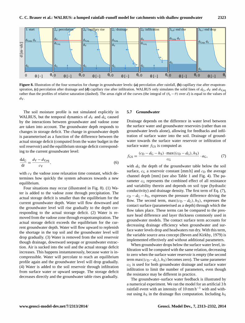
In practice, the soil moisture profile and storage deficit arenever perfectly in equilibrium with the groundwater depth.Addition (e.g. through precipitation) and removal (e.g. bydrainage or evapotranspiration) of water cause an imbal-620

ance between gravity and capillary forces, leading to down-ward (percolation) or upward (capillary rise) flow towardsa new equilibrium situation. Because the flow decreases withproximity to the equilibrium, this equilibrium will only bereached asymptotically.625

The exact profile of relative saturation is not simulated ex-plicitly in WALRUS, but the temporal dynamics of dV anddG caused by the interactions between groundwater and va-dose zone are taken into account. The groundwater depth re-sponds to changes in storage deficit. The change in ground-630

water depth is parameterised as a function of the differencebetween the actual storage deficit (computed from the wa-ter budget in the soil reservoir) and the equilibrium storage

deficit corresponding to the current groundwater level:

ddG

dt=dV− dV,eq

cV, (6)635

with cV the vadose zone relaxation time constant, which de-termines how quickly the system advances towards a newequilibrium.

Four situations may occur (illustrated in Fig. 8). (1) Wa-ter is added to the vadose zone through percolation. The ac-640

tual storage deficit is smaller than the equilibrium for thecurrent groundwater depth. Water will flow downward andthe groundwater level will rise gradually to the depth cor-responding to the actual storage deficit. (2) Water is re-moved from the vadose zone through evapotranspiration. The645

actual storage deficit exceeds the equilibrium for the cur-rent groundwater depth. Water will flow upward to replenishthe shortage in the top soil and the groundwater level willdrop gradually. (3) Water is removed from the soil reservoirthough drainage, downward seepage or groundwater extrac-650

tion. Air is sucked into the soil and the actual storage deficitincreases. This happens instantaneously, because water is in-compressible. Water will percolate to reach an equilibriumprofile again and the groundwater level will drop gradually.(4) Water is added to the soil reservoir through infiltration655

from surface water or upward seepage. The storage deficitdecreases directly and the groundwater table rises gradually.

Figure 7. Relation between groundwater depthdG and storage deficitdV . Coloured lines: data from six and four sites in the two catchments.Dashed black line: relation derived from the Brooks–Corey curve belonging to loamy sand (left) and clay (right). Coloured lines: relationwith b fitted on data. Solid black line: relation with the averageb of the stations. The clouds are represented by the contour lines encompassing70 % of the probability mass estimated using kernel densities (Wand and Jones, 1995).

height above the groundwater tableh [mm] according toClapp and Hornberger(1978) is

θ = θs

(h

ψae

)−1/b

, (4)

with b the pore size distribution parameter [–] andψae the airentry pressure [mm]. The air entry pressure raises the powerlaw distribution above the groundwater table to allow for thecapillary fringe (the saturated area above the groundwater ta-ble). The parametersb, ψae and θs differ per soil type andselected results from laboratory experiments byClapp andHornberger(1978) are given in Table2 (seeCosby et al.,1984, for interpolations between soil types). When the part ofthe profile between the capillary fringe and the soil surfacefrom Eq. (4) is substituted in Eq. (3), the relation betweenequilibrium storage deficit and groundwater depth becomes

dV,eq =

dG∫ψae

[θs− θs

(h

ψae

)−1/b]

dh

= θs

(dG −

d1−1/bG

(1−1b)ψ

−1/bae

−ψae

1− b

). (5)

Heterogeneities, such as soil layering or disruption byplant roots, macrofauna and human activity, cause differ-ences between laboratory and field observations. In Fig.7

dG is plotted as a function ofdV for several sites in theHupsel Brook catchment and Cabauw polder area with cor-responding theoretical curves. We computed the temporalmaximumθ per depth (at the meteorological station in theHupsel Brook catchment and the average of four profiles inthe Cabauw polder) and averaged over the entire measureddepth (205 cm in the Hupsel Brook catchment and 72 cm inthe Cabauw polder) to obtain a single value ofθs. For theHupsel Brook catchment, we fittedb while retainingψae,but for the Cabauw polder it was necessary to fit bothb andψae to obtain curves which describe the data points relativelywell. The values obtained with these fits are listed in Table2.Note that the data are actual storage deficits, which may notbe in equilibrium with the groundwater depth measured atthe same time. In addition, sites differ considerably and willdeviate from the catchment average.

5.6 Percolation and capillary rise

In practice, the soil moisture profile and storage deficit arenever perfectly in equilibrium with the groundwater depth.Addition (e.g. through precipitation) and removal (e.g. bydrainage or evapotranspiration) of water cause an imbal-ance between gravity and capillary forces, leading to down-ward (percolation) or upward (capillary rise) flow towardsa new equilibrium situation. Because the flow decreases withproximity to the equilibrium, this equilibrium will only bereached asymptotically.



0 θs θ [−]

d [m

−sf

c]

dG

dV,eq, dV

1: start

0 θs θ [−]

dG

dV,eq

dV

2a: percolation

0 θs θ [−]

dG

dV,eq

dV

2b: capillary rise

0 θs θ [−]

dG

dV,eq

dV

2c: drainage

0 θs θ [−]

dG

dV,eq

dV

2d: infiltration

0 θs θ [−]

dG

dV,eq, dV

3a,d: end rise

0 θs θ [−]

dG

dV,eq, dV

3b,c: end drop

Figure 8. Illustration of the four scenarios for change in groundwater levels:(a) percolation after rainfall,(b) capillary rise after evapotran-spiration,(c) percolation after drainage and(d) capillary rise after infiltration. WALRUS only simulates the solid lines ofdG, dV anddV,eqrather than the profiles of relative saturation (dashed). The areas right of the curves (the integral of(θs− θ) overd) is equal to the values ofdV .

The soil moisture profile is not simulated explicitly inWALRUS, but the temporal dynamics ofdV anddG causedby the interactions between groundwater and vadose zoneare taken into account. The groundwater depth responds tochanges in storage deficit. The change in groundwater depthis parameterised as a function of the difference between theactual storage deficit (computed from the water budget in thesoil reservoir) and the equilibrium storage deficit correspond-ing to the current groundwater level:

ddG

dt=dV − dV,eq

cV, (6)

with cV the vadose zone relaxation time constant, which de-termines how quickly the system advances towards a newequilibrium.

Four situations may occur (illustrated in Fig.8). (1) Wa-ter is added to the vadose zone through precipitation. Theactual storage deficit is smaller than the equilibrium for thecurrent groundwater depth. Water will flow downward andthe groundwater level will rise gradually to the depth cor-responding to the actual storage deficit. (2) Water is re-moved from the vadose zone through evapotranspiration. Theactual storage deficit exceeds the equilibrium for the cur-rent groundwater depth. Water will flow upward to replenishthe shortage in the top soil and the groundwater level willdrop gradually. (3) Water is removed from the soil reservoirthough drainage, downward seepage or groundwater extrac-tion. Air is sucked into the soil and the actual storage deficitincreases. This happens instantaneously, because water is in-compressible. Water will percolate to reach an equilibriumprofile again and the groundwater level will drop gradually.(4) Water is added to the soil reservoir through infiltrationfrom surface water or upward seepage. The storage deficitdecreases directly and the groundwater table rises gradually.

5.7 Groundwater

Drainage depends on the difference in water level betweenthe surface water and groundwater reservoirs (rather than ongroundwater levels alone), allowing for feedbacks and infil-tration of surface water into the soil. Drainage of ground-water towards the surface water reservoir or infiltration ofsurface waterfGS is computed as

fGS =(cD − dG −hS) · max((cD − dG),hS)

cG· aG, (7)

with dG the depth of the groundwater table below the soilsurface,cG a reservoir constant [mm h] andcD the averagechannel depth [mm] (see also Table1 and Fig.4). The pa-rametercG represents the combined effect of all resistanceand variability therein and depends on soil type (hydraulicconductivity) and drainage density. The first term of Eq. (7),cD − dG −hS, expresses the pressure difference driving theflow. The second term, max((cD − dG),hS), expresses thecontact surface (parameterised as a depth) through which theflow takes place. These terms can be compared to the pres-sure head difference and layer thickness commonly used ingroundwater models. The contact surface term accounts fordecreasing drainage efficiency when groundwater and sur-face water levels drop and headwaters run dry. With this term,the variable source area concept (Beven and Kirkby, 1979) isimplemented effectively and without additional parameters.

When groundwater drops below the surface water level, in-filtration will be computed with the same relation, decreasingto zero when the surface water reservoir is empty (the secondterm max((cD−dG),hS) becomes zero). The same parametercG is used for both groundwater drainage and surface waterinfiltration to limit the number of parameters, even thoughthe resistance may be different in practice.

The groundwater–surface water feedback is illustrated bya numerical experiment. We ran the model for an artificial 3 hrainfall event with an intensity of 10 mm h−1 with and with-out usinghS in the drainage flux computation. IncludinghS



leads to a decrease in drainagefGS and even infiltration (neg-ativefGS) during the peak (Fig.9, left panels). This causesan attenuation of the discharge peak and higher groundwaterlevels after the peak. This feedback is an important character-istic of WALRUS: in most parametric models, surface waterlevels are not modelled explicitly and this feedback cannottake place.

5.8 Quickflow

The quickflow reservoir simulates the combined effect of allwater flowing through quickflow paths towards the surfacewater: overland, macropore and drainpipe flow. This reser-voir can therefore be seen as a collection of ponds, smalldrainage trenches or gulleys, soil cracks, animal burrows anddrainpipes. QuickflowfQS depends linearly on the elevationof the water level in the quickflow reservoirhQ, with a timeconstant (reservoir constant)cQ:

fQS =hQ

cQ· aG. (8)

Water cannot flow from the surface water into the quick-flow reservoir. Therefore, a sudden surface water level risecaused by an increase in surface water supply or weir eleva-tion does not affect the quickflow reservoir directly.

The water level in the quickflow reservoir cannot be cou-pled to measurable variables directly – groundwater levelmeasurements show the combined effect of the seasonal vari-ation of the groundwater depth and the high-resolution dy-namics of the quickflow reservoir. Even though quickflow isparameterised as a single linear reservoir, it is essential toinclude this reservoir to mimic the large and variable contri-bution of these flow routes (see Sect.4.3).

5.9 Surface water

In WALRUS, surface water forms an integral part of themodel structure. The surface water levelhS represents thewater level in the average channel with respect to the chan-nel bottom. The distance between channel bottom and soilsurfacecD is calibrated or estimated from field observations.The stage–discharge relationQ= func(hS) specifies the re-lation between surface water level and discharge at the catch-ment outlet (in mm h−1). It is provided by the user as a func-tion, e.g. the relation belonging to the weir at the catchmentoutlet, or as a lookup table. A threshold levelhS,min can beincluded in the stage–discharge relation to account for a weiror other water management structures. If applicable, a valueor time series ofhS,minshould be provided. When the surfacewater level drops below the crest of a weir, discharge will bezero, but because there may still be drainage, infiltration andevaporation, it is important to include standing water. A de-fault stage–discharge relation with the shape of a power law

00.

51

1.5

Q, f

GS,

f XS

[mm

h−1

]

PQfGS

fXS

with feedbackwithout feedback 10

0

P [m

m h−1

]

10.

5d

[m]

dG

cD−hS

0 1 2 t [d]

0 1 2t [d]

Figure 9. The isolated effect of taking into account thegroundwater–surface water feedback process. Results of a numer-ical experiment with (solid) and without (dashed) using the surfacewater level (hS) in the groundwater drainage flux (fGS) computa-tion. Right panels also include the effect of surface water supply(fXS). For the dashed lines in the left panels,hS was computedwithout fXS andfXS was added to the discharge (Q) afterwards.The same parameter values as in Fig.5 were used.

with a default exponentxS of 1.5 has been implemented:

Q= cS

(hS−hS,min

cD −hS,min

)xS

(9)

for hS ≤ cD. The default exponent value 1.5 forxS is inspiredby equilibrium flow in open channels (Manning, 1889). TheparametercS corresponds to the discharge at the catchmentoutlet (in mm h−1) when the surface water level reaches thesoil surface, comparable to the bankfull discharge. It can becalibrated or provided based on field observations.

5.10 Seepage and surface water supply

All fluxes across the catchment boundary, except for the dis-charge at the catchment outlet, are combined in the externalgroundwater flow termfXG (downward or upward seepageand lateral groundwater inflow or outflow) and the externalsurface water flow termfXS (supply or extraction). Positivevalues denote flow into the catchment. If applicable, time se-ries offXG or fXS should be provided by the user. Seepageand surface water supply are not parameterised, because theydo not depend on processes within the catchment. In the casethat no data are available, a groundwater or surface watermanagement model could be used to obtain time series ofseepage and surface water supply, which can be used as in-put for WALRUS.



Because these fluxes are added to the soil reservoir or sur-face water reservoir, they influence other variables throughthe different feedbacks implemented in the model. Mostparametric rainfall–runoff models do not contain a surfacewater reservoir and therefore surface water supply can onlybe added to discharge afterwards and the impact of surfacewater increase on groundwater level and the groundwaterdrainage flux is not considered.

To investigate the effect of WALRUS’ set-up consider-ing surface water supply, we modelled an artificial eventwith two model set-ups: (1)fXS is added to the surface wa-ter reservoir and groundwater–surface water feedbacks areconsidered (as implemented in WALRUS) and (2)fXS isadded toQ afterwards andhS is not used in the groundwaterdrainage computation. AddingfXS to the surface water reser-voir causes a gradual increase inhS and gradually risingQ(Fig.9, right panels). WhenfXS is added toQ afterwards,hSis not affected byfXS and only increases after rainfall, andQrises and falls instantly after changes infXS. When a largerfraction of the catchment is covered by surface water (aS),the increase inhS andQ becomes more gradual, becausethe supplied surface water volume is spread out over a largersurface. Including the groundwater–surface water feedbackleads to an attenuated discharge peak, caused by a decreasein drainage as a result of a decreasing difference betweendGandhS. In dry periods,fXS may causehS to rise abovedG,leading to infiltration of surface water, which indicates thatseepage and groundwater–surface water feedback should beimplemented together.

5.11 Large-scale ponding and flooding

The quickflow reservoir simulates the effect of local pond-ing and overland flow, but large-scale ponding may also oc-cur. When the storage deficit becomes zero (i.e. all soil poresare filled with water), the groundwater level will rise di-rectly to the surface (as observed byGillham, 1984; Braueret al., 2011). Storage deficit and groundwater depth continueto drop (i.e. become more negative) together as there are nocapillary forces any more and water level and pressure headcoincide – negativedV anddG express ponding depths. Notethat the levels rise less quickly above ground as the storativitybecomes 1.

Unfortunately, few quantitative, catchment-scale observa-tions exist of different fluxes during floods. Because WAL-RUS has no spatial dimensions, the complex process of over-land flow must be simplified. It is assumed that when thegroundwater or surface water level rises above the soil sur-face, the groundwater drainage/surface water infiltration fluxfGS will include overland flow and is instantaneous, becauseoverland flow is much faster than groundwater flow. Whenthe surface water level exceeds the soil surface, dischargebecomes less sensitive to changes in surface water level, rep-resented by an abrupt change in the stage–discharge rela-tion. However, as soon as the surface water level exceeds the

soil surface, the excess water is led to the soil reservoir di-rectly and thereforehS hardly rises above the soil surface.Therefore, we keep the same stage–discharge relation whenhS> cD as a default. When the modelled groundwater tablereaches the soil surface, an abrupt change in catchment dis-charge occurs. This is in contrast to the gradual activationof different flow paths when the catchment effective ground-water table is below surface (as represented by the wetnessindex).

We investigated the option of making the surface waterarea fractionaS a function ofhS, representing gradual widen-ing of brooks and inundation of areas close to the surfacewater network, and thereby smoothing the effect of floodingon discharge at the catchment outlet. Unfortunately, this ap-proach made the model structure less intuitive and introducedmore degrees of freedom to define the shape of this function.Because flooding of the surface water reservoir only occursduring extremely wet situations, we chose to keep the modelstructure simple and leaveaS fixed.

5.12 Outlook: possible model extensions

Some processes are not taken into account in the core modelyet, but a user could easily add preprocessing and postpro-cessing steps to adapt WALRUS to catchment-specific situa-tions. (1) The potential evapotranspiration estimated at a me-teorological station may not be representative for the col-lection of vegetation types in the catchment. Therefore, onecould use land cover distributions and crop factors to de-termine the catchment average potential evapotranspiration.(2) Currently, WALRUS is set up to receive liquid precip-itation, but preprocessing steps to account for snow and/orinterception can be added. For example, the delay in pre-cipitation input caused by snow accumulation and melt canbe simulated with methods based on the land surface en-ergy balance (Kustas et al., 1994) or a degree-day method(Seibert, 1997). (3) Interception can be parameterised witha threshold. Only the rainfall which exceeds the threshold isused as input for the model. The intercepted water evapo-rates directly and is not subtracted from ETpot (Teuling andTroch, 2005). (4) Paved surfaces have a low infiltration ca-pacity, which limits groundwater recharge. This can be pa-rameterised by decreasing the groundwater reservoir areaaG,introducing a paved surface area and leading the fraction ofthe rainfall belonging to this area directly to the surface wa-ter. (5) For large catchments, the discharge pulse from themodel can be delayed and attenuated in the channels. It ispossible to add a routing function to account for the delayand attenuation.

Another possibility is to couple WALRUS to other models.The outflowQ of one catchment can be used as surface wa-ter supplyfXS for another WALRUS unit downstream. Withthis technique, one could make a chain of WALRUS unitsto model subcatchments (with possibly different catchmentcharacteristics and therefore parameter values) separately.



Groundwater flow from one unit to the next can be com-puted from groundwater levels in adjacent cells and Eq. (7).This groundwater flow is added to or subtracted from theseepage fluxfXG for both units. Regional groundwater flowfrom a distributed groundwater model can be added to orsubtracted from the soil reservoir through the seepage fluxfXG. This can be specified with a time series or an exter-nal groundwater level. The outflow of the model can be usedas input for a hydraulic model. Discharge from an upstreamcatchment as computed from a hydraulic model can also beused as inputfXS.

6 Model implementation

In this section we describe some key parts of the model im-plementation, which affect the model application and perfor-mance.

6.1 Code set-up

The model code is written in R, but can be easily translatedinto any vector-oriented interpreted language. The code con-sists of several scripts. Two functions form the core of themodel code:WALRUS_loopandWALRUS_step(provided asSupplement). InWALRUS_loopthe initial conditions are set,a for-loop over each time step is run and output data are or-ganised. For every time step, the functionWALRUS_stepiscalled, which contains the actual model computations. Someadditional scripts (not included in the Supplement, but avail-able upon request) provide help by preprocessing forcingdata, setting default parameters, and postprocessing of themodel output: figures, water balance computations and anal-ysis of residuals. Another script provides a template in whichfunctions are called for preprocessing, calibrating, runningthe model and postprocessing.

6.2 Initial conditions

The model can (as default) compute initial conditions for allstates automatically, based on a stationary situation (therebyavoiding long burn-in periods). The quickflow reservoir isinitially empty. The initial surface water level is derived fromthe first discharge observation and the stage–discharge rela-tion. The initial groundwater depth is computed with the as-sumption that initial groundwater drainage (fGS) is equal tothe initial discharge. It is also possible to supply the fractionof the initial discharge originating from drainageGfrac andthe model will solve

Q0 ·Gfrac =(cD − dG,0 −hS,0) · (cD − dG,0)

cG(10)

for dG,0 with the quadratic formula and then use the remain-der of the discharge to compute the initial quickflow reservoirlevel:

hQ,0 =Q0 · (1−Gfrac) · cQ. (11)

Alternatively, the initial groundwater depth can be sup-plied (or calibrated) by the user andhQ,0 is computed suchthatQ0 = fGS,0 + fQS,0 again. The initial storage deficit isassumed to be the equilibrium value belonging to the initialgroundwater depth.

A user can choose to use a warming-up period in case theuncertainty around the initial conditions is large. It is imple-mented in the code, but by default, the warming-up period isset to zero.

6.3 Parameters

WALRUS has four parameters which require calibration:cW,cV , cG and cQ. These parameters have a physical meaningand can be explained qualitatively with catchment character-istics. The channel depthcD and surface water area fractionaS can be estimated from field observations. When the de-fault stage–discharge relation is used, the bankfull dischargecS and (if applicable) the weir elevationhS,min need to besupplied (or calibrated) as well. Parameters are catchment-specific, but time-independent, to allow a calibrated modelto be run for both long periods and events. We did not im-plement a specific calibration routine in the model, but usedthe HydroPSO package, which is a particle swarm optimi-sation technique (Zambrano-Bigarini and Rojas, 2013). Theuser can define the (multi-)objective function.

6.4 Forcing

Forcing data can be supplied as a time series or as a function(e.g. a sine function for ETpot or a Poisson rainfall genera-tor). Observation times do not need to be equidistant, whichis especially useful for tipping-bucket rain gauges. Forcingtime series are converted to functions (e.g. cumulativeP asfunction of time), which allows other time steps than used forthe original forcing.

6.5 If-statements

If-statements associated with thresholds cause nonlinearitiesin a model and their abrupt changes hamper calibration, inparticular when using gradient-based methods. It is there-fore important to know that there are four causes for abruptchanges in the model: (1) the stage–discharge relation (sup-plied by a user) may show abrupt changes at the elevationof the crest of the weir or at the soil surface; (2) no evap-oration occurs from empty channel beds; (3) if the storagedeficit becomes negative or exceeds the groundwater depth,the groundwater depth becomes equal to the storage deficit;(4) if either groundwater or surface water level exceeds thesoil surface, overland flow is instantaneous.

6.6 Integration scheme

The model is implemented as an explicit scheme, becausenonlinearities caused by feedbacks and if-statements do not



ba

hS,0 hS,1 hS,2 hS,3 hS,4 dG,0 dG,1 dG,2 dG,3 dG,4 ... ... ... ... ...

P1 P2 P3 P4Q1 Q2 Q3 Q4... ... ... ...

P3,1 P3,2 P3,3P3,1Q3,1 Q3,2 Q3,3Q3,1... ... ......

2

11

1

1

3 2 1 1t

Cum

ulat

ive

P

P1

P2

P3,1

P3,2

P3,3

P4

Figure 10. Illustration of the variable time step procedure.(a) Thenon-equidistant output time steps (purple) are used as first attemptsfor computations of fluxes (blue/green) and states (purple), but dur-ing time step number 3, the precipitation sum is too large (panelb)and the step is divided into substeps: it is halved and then halvedagain until the criterion was reached. Note that even though the sizeof output time step 2 is larger, it is not divided into substeps, becauseall criteria are met.

allow for the use of an implicit scheme. The states at the endof the previous time step are used to compute the fluxes dur-ing the current time step, which are then used to compute thestates at the end of the current time step (Fig.10). The outputdata file lists the sums of the fluxes during and the states atthe end of each time step.

6.7 Time step

The user can specify at which moments output should be gen-erated, for example with a fixed interval (i.e. each hour orday), with increased frequency during certain events or aftereach millimetre of rainfall. The output time steps can be bothlarger and smaller than those of the forcing.

An important feature of the model code is the flexible com-putation time step. The model first attempts to run a wholeoutput time step at once, but the time step is decreased when(1) the rainfall sum, discharge sum or change in discharge,surface water level or groundwater depth during the time stepexceeds a certain threshold, or when (2) the surface waterlevel is negative at the end of the time step. The first cri-terion prevents numerical instability caused by the explicitintegration scheme and a delayed the response to rainfall asa result of the explicit model code (it takes one step to updatethe surface water level and another for the discharge). Thesecond criterion is necessary because the total surface wateroutflow, computed from water levels at the start of the timestep and the time step size, can exceed the available water.Because this means that non-existing water flowed out, thereis a physical reason to avoid this.

The procedure of decreasing time steps is illustrated inFig. 10 (third step). First the original time step is halved andthe model is run for this substep (of course with the forcingcorresponding to this substep). When the criteria are still notmet, the step size will be halved again and again until the

0 6 15 18

01

2

t [h]

Q [m

m h

−1]

●●

●

●

●● ●

●●

●●

●●

● ● ● ● ●

● ●

●

●

●● ●

●●

●●

●●

● ● ● ● ●

●

●

∆t=1h∆t=1h, no substeps∆t=3h∆t=3h, no substeps

P =

30

mm

Figure 11. The effect of variable time steps on the model output.An artificial case with a rainfall event of 30 mm in the first hour andno evapotranspiration. The lines connect the discharge modelled atthe end of a time step (instantaneous value), and do not representthe sum over the time step (which is given in the output file). Thesame parameter values as in Fig.5 were used.

criteria are met. When one substep is completed, the fluxesare stored and the states at the end of the time step are used asinitial values for the next substep. Then the model is run forthe remainder of the original time step and, if necessary, thesubstep is halved until the criteria are met. This will continueuntil the end of the intended output time step is reached. Thesum of the fluxes of the substeps and the states of the lastsubstep are stored in the output file.

The effect of the variable time step is illustrated in Fig.11,in which the output of the model run with a fixed time stepand with variable time steps is shown. Note the erroneoustime delay and magnitude of the discharge peak when nosubsteps are used, in particular for the 3-hourly time step.

6.8 Water balance

WALRUS is a mass conserving model, and therefore themodel water budget, computed as

6P −6ETact−6Q+6fXG +6fXS =

−1dV · aG +1hQ · aG +1hS · aS, (12)

always closes, although rounding errors may cause small de-viations. The minus sign before1dV appears becausedV ex-presses a deficit and a decrease in storage deficit implies anincrease in water in the reservoir. The groundwater level doesnot appear explicitly in the water balance, because it onlyplays a role as a pressure level driving groundwater drainageand surface water infiltration fluxes, while the storage deficitaccounts for volume changes in the whole soil reservoir.

7 Conclusions

The Wageningen Lowland Runoff Simulator (WALRUS)is a new rainfall–runoff model, which is suitable for low-lands where shallow groundwater and surface water influ-ence runoff generation. The model explicitly accounts for



processes which are typically not included in parametric rain-fall runoff models, but which are important in lowland areas:

1. Groundwater–unsaturated zone coupling– WALRUScontains one soil reservoir, which is divided effectivelyby the (dynamic) groundwater table into a groundwaterzone and a vadose zone. The condition of this soil reser-voir is described by two strongly dependent variables:the groundwater depth and the storage deficit (the effec-tive thickness of empty pores). This implementation en-ables capillary rise when the top soil has dried throughevapotranspiration.

2. Wetness-dependent flow routes– the storage deficitdetermines the division of rain water between thesoil reservoir (slow routes: infiltration, percolation andgroundwater flow) and a quickflow reservoir (quickroutes: drainpipe, macropore and overland flow).

3. Groundwater–surface water feedbacks– surface waterforms an explicit part of the model structure. Drainagedepends on the difference between surface water leveland groundwater level (rather than groundwater levelalone), allowing for feedbacks and infiltration of surfacewater into the soil.

4. Seepage and surface water supply– groundwater seep-age and surface water supply or extraction (pumping)are added to or subtracted from the soil or surface waterreservoir. These external fluxes affect the whole systemthrough the groundwater–surface water feedbacks andsaturated-unsaturated zone coupling.

The open-source model code is implemented in R andthe model is set up such that it can be used by both prac-titioners and researchers. For direct use by practitioners, de-faults are implemented for relations between model variablesand to compute initial conditions, leaving only four param-eters which require calibration. For research purposes, thedefaults can easily be changed. WALRUS is computation-ally efficient, which allows operational forecasting and un-certainty estimation by creating ensembles. An approach forflexible time steps increases numerical stability and makesmodel parameter values independent of time step size, whichfacilitates use of the model with the same parameter set formulti-year water balance studies as well as detailed analysesof individual flood peaks.

Numerical experiments shows that the implemented feed-backs have the desired effect on the system variables: (1) thewetness-dependent division between slow and quickflowroutes results in more quickflow, less recharge and higher dis-charge peaks during wet periods; (2) the surface water levelattenuates drainage during discharge peaks or when surfacewater is supplied upstream. An exhaustive test of WALRUS,with calibration, several validation studies, sensitivity anal-yses and uncertainty analyses in two catchments, the freelydraining Hupsel Brook catchment and the controlled Cabauw

polder, is presented in a companion paper (Brauer et al.,2014).

Compared to other rainfall–runoff models, WALRUS hassome important advantages: it (1) is applicable to both freelydraining and polder areas, (2) is computationally efficient,(3) has few parameters (only four to calibrate), (4) has aclear (qualitative) relation between model states and measur-able variables, (5) has default options for initial conditionsand parameterisations (which can easily be changed for re-search purposes), and (6) is open source and freeware (pro-grammed in R). These advantages make WALRUS suitablefor operational flood and drought forecasting, real-time con-trol, input for hydraulic models, risk analyses, scenario anal-yses, infrastructure design and time series gap filling in low-land catchments. In that sense, WALRUS complements exist-ing rainfall–runoff models, containing the core hydrologicalprocesses for lowlands, while maintaining a simple modelstructure. This makes WALRUS suitable for discharge simu-lations by researchers and practitioners alike.

Code availability

The complete model code can be obtained upon request (byemailing the first author). In addition, the code will be madeavailable through the R CRAN website. WALRUS is licensedunder the GPL v3 licence.

The Supplement related to this article is available onlineat doi:10.5194/gmd-7-2313-2014-supplement.

Acknowledgements.We thank Piet Warmerdam and Han Strickerfor sharing their experience with the Wageningen model. We thankRoel Velner (Water Board Rivierenland), Gert van den Houten andMarian Koskamp (Water Board Rijn and IJssel), Frank Weerts(Water Board De Dommel), Jos Moorman (Water Board Aa andMaas), Jan Gooijer (Water Board Noorderzijlvest), Siebe Boschand Ralph Pieters Kwiers (HydroConsult) and Klaas-Jan vanHeeringen and Govert Verhoeven (Deltares) for their valuable in-sights from the end-user’s perspective. We thank KNMI (especiallyFred Bosveld) for evapotranspiration data in the Cabauw polder,the Water Board Rijn and IJssel for discharge and water qualitydata of the Hupsel Brook catchment and Rijkswaterstaat for soilmoisture and groundwater data in the Hupsel Brook catchment.We thank Han Stricker, Jantine Bokhorst, Wilco Terink, MatthijsBoersema, Jacques Warmer, Wim Hovius and Marcel Brinkenbergfor help with the field work in the Cabauw polder.

Edited by: J. Neal


http://dx.doi.org/10.5194/gmd-7-2313-2014-supplement


References

Abbott, M. B., Bathurst, J. C., Cunge, J. A., O’Connell, P. E., andRasmussen, J.: An introduction to the European HydrologicalSystem-Système Hydrologique Européen, “SHE”, 1: History andphilosophy of a physically-based, distributed modelling system,J. Hydrol., 87, 45–59, 1986.

Appels, W. M.: Water redistribution at the soil surface: ponding andsurface runoff in flat areas, Ph.D. thesis, Wageningen University,2013.

Appels, W. M., Bogaart, P. W., and van der Zee, S. E. A. T. M.: In-fluence of spatial variations of microtopography and infiltrationon surface runoff and field scale hydrological connectivity, Adv.Water Resour., 34, 303–313, 2011.

Arnold, J. G., Srinivasan, R., Muttiah, R. S., and Williams, J. R.:Large area hydrologic modeling and assessment – Part 1: Modeldevelopment, J. Am. Water Resour. As., 34, 73–89, 1998.

Beljaars, A. C. M. and Bosveld, F. C.: Cabauw data for the vali-dation of land surface parameterization schemes, J. Climate, 10,1172–1193, 1997.

Bergström, S. and Forsman, A.: Development of a conceptual deter-ministic rainfall–runoff model, Nord. Hydrol., 4, 147–170, 1973.

Beven, K.: Changing ideas in hydrology – the case of physically-based models, J. Hydrol., 105, 157–172, 1989.

Beven, K.: Linking parameters across scales: subgrid parameteriza-tions and scale dependent hydrological models, Hydrol. Process.,9, 507–525, 1995.

Beven, K. J. and Binley, A. M.: The future of distributed models:model calibration and uncertainty prediction, Hydrol. Process.,6, 297–298, 1992.

Beven, K. and Freer, J.: A dynamic topmodel, Hydrol. Process., 15,1993–2011, 2001.

Beven, K. and Germann, P.: Macropores and water flow in soils,Water Resour. Res., 18, 1311–1325, 1982.

Beven, K. and Germann, P.: Macropores and water flow in soilsrevisited, Water Resour. Res., 49, 3071–3092, 2013.

Beven, K. J. and Kirkby, M. J.: A physically based, variable con-tributing area model of basin hydrology, Hydrol. Sci. J., 24, 43–69, 1979.

Bogaart, P. W., Teuling, A. J., and Troch, P. A.: A state-dependentparameterization of saturated-unsaturated zone interaction, Wa-ter Resour. Res., 44, W11423, doi:10.1029/2007WR006487,2008.

Bormann, H. and Elfert, S.: Application of WaSiM-ETH model toNorthern German lowland catchments: model performance inrelation to catchment characteristics and sensitivity to land usechange, Adv. Geosci., 27, 1–10, doi:10.5194/adgeo-27-1-2010,2010.

Brauer, C. C., Teuling, A. J., Overeem, A., van der Velde, Y., Hazen-berg, P., Warmerdam, P. M. M., and Uijlenhoet, R.: Anatomy ofextraordinary rainfall and flash flood in a Dutch lowland catch-ment, Hydrol. Earth Syst. Sci., 15, 1991–2005, doi:10.5194/hess-15-1991-2011, 2011.

Brauer, C. C., Teuling, A. J., Torfs, P. J. J. F., and Uijlenhoet, R.:Investigating storage–discharge relations in a lowland catchmentusing hydrograph fitting, recession analysis, and soil moisturedata, Water Resour. Res., 49, 4257–4264, 2013.

Brauer, C. C., Torfs, P. J. J. F., Teuling, A. J., and Uijlenhoet, R.:The Wageningen Lowland Runoff Simulator (WALRUS): appli-cation to the Hupsel Brook catchment and the Cabauw polder,

Hydrol. Earth Syst. Sci., 18, 4007–4028, doi:10.5194/hess-18-4007-2014, 2014.

Brooks, R. H. and Corey, A. T.: Hydraulic properties of porous me-dia, Hydrology Paper 3, Colorado State University, Fort Collins,CO, 27 pp., 1964.

Brunner, G. W.: HEC-RAS River Analysis System. Hydraulic Ref-erence Manual. Version 1.0., Tech. rep., DTIC Document, USArmy Corps of Engineers, Davis, USA, 1995.

Burnash, R. J. C.: The NWS river forecast system – catchment mod-eling, in: Computer Models of Watershed Hydrology, edited by:Singh, V. P., Water Resour. Publ., Highlands Ranch, Colorado,USA, 311–366, 1995.

Canadell, J., Jackson, R. B., Ehleringer, J. B., Mooney, H. A.,Sala, O. E., and Schulze, E. D.: Maximum rooting depth of veg-etation types at the global scale, Oecologia, 108, 583–595, 1996.

Chen, X. and Hu, Q.: Groundwater influences on soil moisture andsurface evaporation, J. Hydrol., 297, 285–300, 2004.

Clapp, R. B. and Hornberger, G. M.: Empirical equations for somehydraulic properties, Water Resour. Res., 14, 601–604, 1978.

Clark, M. P., Slater, A. G., Rupp, D. E., Woods, R. A., Vrugt, J. A.,Gupta, H. V., Wagener, T., and Hay, L. E.: Framework for Under-standing Structural Errors (FUSE): a modular framework to di-agnose differences between hydrological models, Water Resour.Res., 44, W00B02, doi:10.1029/2007WR006735, 2008.

Cosby, B. J., Hornberger, G. M., Clapp, R. B., and Ginn, T. R.:A statistical exploration of the relationships of soil moisture char-acteristics to the physical properties of soils, Water Resour. Res.,20, 682–690, 1984.

Delsman, J. R., Oude Essink, G. H. P., Beven, K. J., andStuyfzand, P. J.: Uncertainty estimation of end-member mixingusing generalized likelihood uncertainty estimation (GLUE), ap-plied in a lowland catchment, Water Resour. Res., 49, 4792–4806, 2013.

Deltares: SOBEK, 1D/2D modelling suite for integral water so-lutions: hydrodynamics, rainfall runoff and real-time control,Deltares, Delft, available at:www.deltares.nl(last access: 1September 2014), 2013.

Dunne, T. and Black, R. D.: Partial area contributions to stormrunoff in a small New England watershed, Water Resour. Res.,6, 1296–1311, 1970.

Edijatno, de Oliveira Nascimento, N., Yang, X., Makhlouf, Z., andMichel, C.: GR3J: a daily watershed model with three free pa-rameters, Hydrol. Sci. J., 44, 263–277, 1999.

Efstratiadis, A. and Koutsoyiannis, D.: One decade of multi-objective calibration approaches in hydrological modelling: a re-view, Hydrol. Sci. J., 55, 58–78, 2010.

Fan, Y., Li, H., and Miguez-Macho, G.: Global patterns of ground-water table depth, Science, 339, 940–943, 2013.

Fenicia, F., Savenije, H. H. G., Matgen, P., and Pfister, L.: Isthe groundwater reservoir linear? Learning from data in hy-drological modelling, Hydrol. Earth Syst. Sci., 10, 139–150,doi:10.5194/hess-10-139-2006, 2006.

Fenicia, F., Kavetski, D., and Savenije, H. H. G.: Elements ofa flexible approach for conceptual hydrological modeling: 1. Mo-tivation and theoretical development, Water Resour. Res., 47,W11510, doi:10.1029/2010WR010174, 2011.

Gillham, R. W.: The capillary fringe and its effect on water-tableresponse, J. Hydrol., 67, 307–324, 1984.


http://dx.doi.org/10.1029/2007WR006487

http://dx.doi.org/10.5194/adgeo-27-1-2010

http://dx.doi.org/10.5194/hess-15-1991-2011




http://dx.doi.org/10.1029/2007WR006735

www.deltares.nl


http://dx.doi.org/10.1029/2010WR010174


Gupta, H. V., Sorooshian, S., and Yapo, P. O.: Toward improved cal-ibration of hydrologic models: multiple and noncommensurablemeasures of information, Water Resour. Res., 34, 751–763, 1998.

Hall, F. R.: Base-flow recessions – a review, Water Resour. Res., 4,973–983, 1968.

Hansen, A. L., Refsgaard, J. C., Christensen, B. S. B., andJensen, K. H.: Importance of including small-scale tile drain dis-charge in the calibration of a coupled groundwater-surface watercatchment model, Water Resour. Res., 49, 585–603, 2013.

Herrmann, A. and Duncker, D.: Runoff formation in a tile-drainedagricultural basin of the Harz Mountain foreland, northern Ger-many, Soil Water Res., 3, 83–97, 2008.

Hopmans, J. and van Immerzeel, C.: Variation in evapotranspirationand capillary rise with changing soil profile characteristics, Agr.Water Manage., 13, 295–305, 1988.

Jakeman, A. J. and Hornberger, G. M.: How much complexity iswarranted in a rainfall–runoff model?, Water Resour. Res., 29,2637–2649, 1993.

Jarvis, N. J.: A simple empirical model of root water uptake, J. Hy-drol., 107, 57–72, 1989.

Kirchner, J.: Getting the right answers for the right reasons:linking measurements, analyses, and models to advance thescience of hydrology, Water Resour. Res., 42, W03S04,doi:10.1029/2005WR004362, 2006.

Kirchner, J. W.: Catchments as simple dynamical systems:catchment characterization, rainfall–runoff modeling, and do-ing hydrology backwards, Water Resour. Res., 45, W02429,doi:10.1029/2008WR006912, 2009.

Koch, S., Bauwe, A., and Lennartz, B.: Application of the SWATModel for a tile-drained lowland catchment in north-eastern Ger-many on subbasin scale, Water Resour. Manag., 27, 791–805,2013.

Koster, R. D., Suarez, M. J., Ducharne, A., Stieglitz, M., and Ku-mar, P.: A catchment-based approach to modeling land surfaceprocesses in a general circulation model: 1. Model structure, J.Geophys. Res.-Atmos., 105, 24809–24822, 2000.

Krause, S. and Bronstert, A.: The impact of groundwater–surfacewater interactions on the water balance of a mesoscale lowlandriver catchment in northeastern Germany, Hydrol. Process., 21,169–184, 2007.

Krause, S., Bronstert, A., and Zehe, E.: Groundwater–surface waterinteractions in a North German lowland floodplain – implicationsfor the river discharge dynamics and riparian water balance, J.Hydrol., 347, 404–417, 2007.

Krzysztofowicz, R.: The case for probabilistic forecasting in hy-drology, J. Hydrol., 249, 2–9, 2001.

Kustas, W. P., Rango, A., and Uijlenhoet, R.: A simple energy bud-get algorithm for the snowmelt runoff model, Water Resour. Res.,30, 1515–1527, 1994.

Lasserre, F., Razack, M., and Banton, O.: A GIS-linked model forthe assessment of nitrate contamination in groundwater, J. Hy-drol., 224, 81–90, 1999.

Liang, X., Lettenmaier, D. P., and Wood, E. F.: One-dimensionalstatistical dynamic representation of subgrid spatial variabilityof precipitation in the two-layer variable infiltration capacitymodel, J. Geophys. Res., 101, 21403–21421, 1996.

Liu, Y., Weerts, A. H., Clark, M., Hendricks Franssen, H.-J., Ku-mar, S., Moradkhani, H., Seo, D.-J., Schwanenberg, D., Smith, P.,van Dijk, A. I. J. M., van Velzen, N., He, M., Lee, H., Noh, S. J.,

Rakovec, O., and Restrepo, P.: Advancing data assimilation inoperational hydrologic forecasting: progresses, challenges, andemerging opportunities, Hydrol. Earth Syst. Sci., 16, 3863–3887,doi:10.5194/hess-16-3863-2012, 2012.

Makkink, G. F.: Testing the Penman formula by means of lysime-ters, Int. J. Water. Eng., 11, 277–288, 1957.

Manning, R.: On the flow of water in open channels and pipes,Trans. Inst. Civ. Eng. Ireland, 20, 161–207, 1889.

McDonald, M. G. and Harbaugh, A. W.: A modular three-dimensional finite-difference ground-water flow model, USGSNumbered Series 83–875, US Geological Survey, Denver, USA,1984.

McDonnell, J. J.: Where does water go when it rains? Moving be-yond the variable source area concept of rainfall–runoff response,Hydrol. Process., 17, 1869–1875, 2003.

McDonnell, J. J., Sivapalan, M., Vaché, K., Dunn, S., Grant, G.,Haggerty, R., Hinz, C., Hooper, R., Kirchner, J., and Roder-ick, M. L.: Moving beyond heterogeneity and process complex-ity: a new vision for watershed hydrology, Water Resour. Res.,43, W07301, doi:10.1029/2006WR005467, 2007.

Moore, R. J.: The probability-distributed principle and runoff pro-duction at point and basin scales, Hydrolog. Sci. J., 30, 273–297,1985.

Moore, R. J.: The PDM rainfall-runoff model, Hydrol. Earth Syst.Sci., 11, 483–499, doi:10.5194/hess-11-483-2007, 2007.

Mosley, M. P.: Streamflow generation in a forested watershed, NewZealand, Water Resour. Res., 15, 795–806, 1979.

Perrin, C., Michel, C., and Andréassian, V.: Does a large num-ber of parameters enhance model performance? Comparative as-sessment of common catchment model structures on 429 catch-ments, J. Hydrol., 242, 275–301, 2001.

Perrin, C., Michel, C., and Andréassian, V.: Improvement of a parsi-monious model for streamflow simulation, J. Hydrol., 279, 275–289, 2003.

Prinsen, G. F. and Becker, B. P. J.: Application of Sobek hydraulicsurface water models in the Netherlands hydrological modellinginstrument, Irrig. Drain., 60, 35–41, 2011.

Querner, E. P.: Description of a regional groundwater flow modelSIMGRO and some applications, Agr. Water Manage., 14, 209–218, 1988.

Rakovec, O., Weerts, A. H., Hazenberg, P., Torfs, P. J. J. F.,and Uijlenhoet, R.: State updating of a distributed hydrologicalmodel with Ensemble Kalman Filtering: effects of updating fre-quency and observation network density on forecast accuracy,Hydrol. Earth Syst. Sci., 16, 3435–3449, doi:10.5194/hess-16-3435-2012, 2012.

Refsgaard, J. C. and Storm, B.: MIKE SHE, in: Computer Modelsof Watershed Hydrology, edited by: Singh, V., Water ResourcesPublications, Colorado, USA, 809–846, 1995.

Rozemeijer, J. C., van der Velde, Y., van Geer, F. C.,Bierkens, M. F. P., and Broers, H. P.: Direct measurements ofthe tile drain and groundwater flow route contributions to surfacewater contamination: from field-scale concentration patterns ingroundwater to catchment-scale surface water quality, Environ.Pollut., 158, 3571–3579, 2010a.

Rozemeijer, J. C., van der Velde, Y., van Geer, F. C., de Rooij, G. H.,Torfs, P. J. J. F., and Broers, H. P.: Improving load estimates forNO3 and P in surface waters by characterizing the concentra-


http://dx.doi.org/10.1029/2005WR004362

http://dx.doi.org/10.1029/2008WR006912


http://dx.doi.org/10.1029/2006WR005467





tion response to rainfall events, Environ. Sci. Technol., 44, 6305–6312, 2010b.

Schenk, H. J. and Jackson, R. B.: The global biogeography of roots,Ecol. Monogr., 72, 311–328, 2002.

Schulla, J. and Jasper, K.: Model Description WaSiM-ETH, Insti-tute for Atmospheric and Climate Science, Swiss Federal Insti-tute of Technology, Zürich, 2007.

Seibert, J.: Estimation of parameter uncertainty in the HBV model,Nord. Hydrol., 28, 247–262, 1997.

Seibert, J.: Multi-criteria calibration of a conceptual runoff modelusing a genetic algorithm, Hydrol. Earth Syst. Sci., 4, 215–224,doi:10.5194/hess-4-215-2000, 2000.

Seibert, J. and McDonnell, J. J.: On the dialog between experimen-talist and modeler in catchment hydrology: use of soft data formulticriteria model calibration, Water Resour. Res., 38, 1241,doi:10.1029/2001WR000978, 2002.

Šimunek, J., van Genuchten, M. T., and Šejna, M.: The HYDRUS-1D software package for simulating the one-dimensional move-ment of water, heat, and multiple solutes in variably-saturatedmedia, Tech. Rep. 3, KNMI, The Bilt, The Netherlands, 2008.

Sophocleous, M. and Perkins, S. P.: Methodology and applicationof combined watershed and ground-water models in Kansas, J.Hydrol., 236, 185–201, 2000.

Soulsby, C., Rodgers, P. J., Petry, J., Hannah, D. M., Malcolm, I. A.,and Dunn, S. M.: Using tracers to upscale flow path understand-ing in mesoscale mountainous catchments: two examples fromScotland, J. Hydrol., 291, 174–196, 2004.

Soulsby, C., Neal, C., Laudon, H., Burns, D. A., Merot, P.,Bonell, M., Dunn, S. M., and Tetzlaff, D.: Catchment data forprocess conceptualization: simply not enough?, Hydrol. Process.,22, 2057–2061, 2008.

Stenitzer, E., Diestel, H., Zenker, T., and Schwartengräber, R.: As-sessment of capillary rise from shallow groundwater by the sim-ulation model SIMWASER using either estimated pedotrans-fer functions or measured hydraulic parameters, Water Resour.Manag., 21, 1567–1584, 2007.

Stricker, J. N. M. and Brutsaert, W.: Actual evapotranspiration overa summer in the Hupsel Catchment, J. Hydrol., 39, 139–157,1978.

Stricker, J. N. M. and Warmerdam, P. M. M.: Estimation of the wa-ter balance in the Hupselse Beek basin over a period of threeyears and a first effort to simulate the rainfall–runoff process fora complete year, in: Proceedings of the International symposiumon hydrological research basins and their use in water resourcesplanning, 21–23 September 1982, Bern, Switzerland, 379–388,1982.

Sugawara, M., Ozaki, E., Watanabe, I., and Katsuyama, Y.: TankModel and its Application to Bird Creek, Wollombi Brook, BikinRiver, Kitsu River, Sanaga River and Nam Mune, vol. 11, Na-tional Research Center for Disaster Prevention, Tsukuba, Japan,1974.

Te Brake, B., van der Ploeg, M. J., and de Rooij, G. H.: Wa-ter storage change estimation from in situ shrinkage measure-ments of clay soils, Hydrol. Earth Syst. Sci., 17, 1933–1949,doi:10.5194/hess-17-1933-2013, 2013.

Tetzlaff, D., Soulsby, C., Waldron, S., Malcolm, I. A., Bacon, P. J.,Dunn, S. M., Lilly, A., and Youngson, A. F.: Conceptualizationof runoff processes using a geographical information system and

tracers in a nested mesoscale catchment, Hydrol. Process., 21,1289–1307, 2007.

Teuling, A. J. and Troch, P. A.: Improved understanding of soilmoisture variability dynamics, Geophys. Res. Lett., 32, L05404,doi:10.1029/2004GL021935, 2005.

Teuling, A. J., Uijlenhoet, R., Hupet, F., and Troch, P. A.: Impact ofplant water uptake strategy on soil moisture and evapotranspira-tion dynamics during drydown, Geophys. Res. Lett., 33, L03401,doi:10.1029/2005GL025019, 2006.

Therrien, R., McLaren, R. G., Sudicky, E. A., and Panday, S. M.:HydroGeoSphere: A Three-Dimensional Numerical Model De-scribing Fully-Integrated Subsurface and Surface Flow and So-lute Transport, Groundwater Simul. Group, Waterloo, Ont.,Canada, 2006.

Thom, A. and Oliver, H.: On Penman’s equation for estimating re-gional evaporation, Q. J. Roy. Meteor. Soc., 103, 345–357, 1977.

Tiemeyer, B., Moussa, R., Lennartz, B., and Voltz, M.: MHYDAS-DRAIN: a spatially distributed model for small, artificiallydrained lowland catchments, Ecol. Model., 209, 2–20, 2007.

Todini, E.: The ARNO rainfall–runoff model, J. Hydrol., 175, 339–382, 1996.

Tromp-van Meerveld, H. J. and McDonnell, J. J.: Threshold rela-tions in subsurface stormflow: 2. The fill and spill hypothesis,Water Resour. Res., 42, W02411, doi:10.1029/2004WR003800,2006.

Turunen, M., Warsta, L., Paasonen-Kivekäs, M., Nurminen, J.,Myllys, M., Alakukku, L., Äijö, H., Puustinen, M., andKoivusalo, H.: Modeling water balance and effects of differentsubsurface drainage methods on water outflow components ina clayey agricultural field in boreal conditions, Agr. Water Man-age., 121, 135–148, 2013.

Uhlenbrook, S., Seibert, J., Leibundgut, C., and Rodhe, A.: Predic-tion uncertainty of conceptual rainfall–runoff models caused byproblems in identifying model parameters and structure, Hydrol.Sci. J., 44, 779–797, 1999.

Van Andel, S. J., Price, R., Lobbrecht, A., and van Kruiningen, F.:Modeling controlled water systems, J. Irrig. Drain. E.-ASCE,136, 392–404, 2010.

Van Dam, J. C., Groenendijk, P., Hendriks, R. F. A., andKroes, J. G.: Advances of modeling water flow in variably sat-urated soils with SWAP, Vadose Zone J., 7, 640–653, 2008.

Van den Eertwegh, G. A. P. H., Nieber, J. L., de Louw, P. G. B., vanHardeveld, H. A., and Bakkum, R.: Impacts of drainage activitiesfor clay soils on hydrology and solute loads to surface water,Irrig. Drain., 55, 235–245, 2006.

Van der Ploeg, M. J., Appels, W. M., Cirkel, D. G., Ooster-woud, M. R., Witte, J.-P. M., and van der Zee, S. E. A. T. M.:Microtopography as a driving mechanism for ecohydrologicalprocesses in shallow groundwater systems, Vadose Zone J., 11,doi:10.2136/vzj2011.0098, 2012.

Van der Velde, Y., de Rooij, G. H., and Torfs, P. J. J. F.:Catchment-scale non-linear groundwater-surface water interac-tions in densely drained lowland catchments, Hydrol. Earth Syst.Sci., 13, 1867–1885, doi:10.5194/hess-13-1867-2009, 2009.

Van der Velde, Y., de Rooij, G. H., Rozemeijer, J. C., vanGeer, F. C., and Broers, H. P.: Nitrate response of a low-land catchment: on the relation between stream concentrationand travel time distribution dynamics, Water Resour. Res., 46,W11534, doi:10.1029/2010WR009105, 2010a.



http://dx.doi.org/10.1029/2001WR000978


http://dx.doi.org/10.1029/2004GL021935

http://dx.doi.org/10.1029/2005GL025019

http://dx.doi.org/10.1029/2004WR003800

http://dx.doi.org/10.2136/vzj2011.0098


http://dx.doi.org/10.1029/2010WR009105


Van der Velde, Y., Rozemeijer, J. C., de Rooij, G. H., van Geer, F. C.,and Broers, H. P.: Field-scale measurements for separationof catchment discharge into flow route contributions, VadoseZone J., 9, 25–35, 2010b.

Van der Velde, Y., Rozemeijer, J. C., de Rooij, G. H., van Geer, F. C.,Torfs, P. J. J. F., and de Louw, P. G. B.: Improving catchmentdischarge predictions by inferring flow route contributions froma nested-scale monitoring and model setup, Hydrol. Earth Syst.Sci., 15, 913–930, doi:10.5194/hess-15-913-2011, 2011.

Van Genuchten: A closed-form equation for predicting the hy-draulic conductivity of unsaturated soils, Soil Sci. Soc. Am. J.,44, 892–898, 1980.

Van Walsum, P. E. V. and Groenendijk, P.: Quasi steady-state sim-ulation of the unsaturated zone in groundwater modeling of low-land regions, Vadose Zone J., 7, 769–781, 2008.

Van Walsum, P. E. V., and Veldhuizen, A. A.: Integration of modelsusing shared state variables: implementation in the regional hy-drologic modelling system SIMGRO, J. Hydrol., 409, 363–370,2011.

Vrugt, J. A., Diks, C. G., Gupta, H. V., Bouten, W., and Ver-straten, J. M.: Improved treatment of uncertainty in hydro-logic modeling: combining the strengths of global optimiza-tion and data assimilation, Water Resour. Res., 41, W01017,doi:10.1029/2004WR003059, 2005.

Vrugt, J. A., ter Braak, C. J. F., Clark, M. P., Hyman, J. M.,and Robinson, B. A.: Treatment of input uncertainty in hy-drologic modeling: doing hydrology backward with Markovchain Monte Carlo simulation, Water Resour. Res., 44, W00B09,doi:10.1029/2007WR006720, 2008.

Wagener, T.: Evaluation of catchment models, Hydrol. Process., 17,3375–3378, 2003.

Wagener, T. and Wheater, H. S.: Rainfall–Runoff Modelling inGauged and Ungauged Catchments, Imperial College Press, Lon-don, UK, 2004.

Wagener, T., Boyle, D. P., Lees, M. J., Wheater, H. S., Gupta, H. V.,and Sorooshian, S.: A framework for development and applica-tion of hydrological models, Hydrol. Earth Syst. Sci., 5, 13–26,doi:10.5194/hess-5-13-2001, 2001.

Wand, M. and Jones, M.: Kernel Smoothing, Chapman and Hall,London, 1995.

Weiler, M. and McDonnell, J.: Virtual experiments: a new ap-proach for improving process conceptualization in hillslope hy-drology, J. Hydrol., 285, 3–18, 2004.

Weir, A. H. and Barraclough, P. B.: The effect of drought on theroot growth of winter wheat and on its water uptake from a deeploam, Soil Use Manage., 2, 91–96, 1986.

Zambrano-Bigarini, M. and Rojas, R.: A model-independent parti-cle swarm optimisation software for model calibration, Environ.Modell. Softw., 43, 5–25, 2013.

Zencich, S. J., Froend, R. H., Turner, J. V., and Gailitis, V.: Influenceof groundwater depth on the seasonal sources of water accessedby Banksia tree species on a shallow, sandy coastal aquifer, Oe-cologia, 131, 8–19, 2002.

Zeng, F., Song, C., Guo, H., Liu, B., Luo, W., Gui, D., Arndt, S.,and Guo, D.: Responses of root growth of Alhagi sparsifoliaShap. (Fabaceae) to different simulated groundwater depths inthe southern fringe of the Taklimakan Desert, China, J. AridLand, 5, 220–232, 2013.



http://dx.doi.org/10.1029/2004WR003059

http://dx.doi.org/10.1029/2007WR006720


the wageningen lowland runoff simulator (walrus… · the wageningen lowland runoff simulator...

Documents