the value of information sharing in a two-stage supply...

The Value of Information Sharing in a Two-Stage SupplyChain with Production Capacity Constraints

David Simchi-Levi,1 Yao Zhao2

1 The Engineering Systems Division and the Department of Civil and EnvironmentalEngineering, Massachusetts Institute of Technology, Cambridge, Massachusetts 02139-4307

2 Department of Management Science and Information Systems, Rutgers University,Newark, New Jersey 07102-1895

Received 23 May 2001; revised 7 April 2003; accepted 7 April 2003

DOI 10.1002/nav.10094

Abstract: We consider a simple two-stage supply chain with a single retailer facing i.i.d.demand and a single manufacturer with finite production capacity. We analyze the value ofinformation sharing between the retailer and the manufacturer over a finite time horizon. In ourmodel, the manufacturer receives demand information from the retailer even during time periodsin which the retailer does not order. To analyze the impact of information sharing, we considerthe following three strategies: (1) the retailer does not share demand information with themanufacturer; (2) the retailer does share demand information with the manufacturer and themanufacturer uses the optimal policy to schedule production; (3) the retailer shares demandinformation with the manufacturer and the manufacturer uses a greedy policy to scheduleproduction. These strategies allow us to study the impact of information sharing on themanufacturer as a function of the production capacity, and the frequency and timing in whichdemand information is shared. © 2003 Wiley Periodicals, Inc. Naval Research Logistics 50: 888–916,2003.

Keywords: production-inventory systems; capacity constraint; information sharing; optimalpolicies; dynamic programming

1. INTRODUCTION

Information technology is an important enabler of efficient supply chain strategies. Indeed,much of the current interest in supply chain management is motivated by the possibilitiesintroduced by the abundance of data and the savings inherent in sophisticated analysis of thesedata. For example, information technology has changed the way companies interact withsuppliers and customers. Strategic partnering, which relies heavily on information sharing, isbecoming ubiquitous in many industries.

Correspondence to: D. Simchi-Levi

© 2003 Wiley Periodicals, Inc.

As observed by Stein and Sweat [9], sharing demand information vertically among supplychain members has achieved huge success in practice. According to Stein and Sweat, by“exchanging information, such as inventory level, forecasting data, and sales trends, thesecompanies are reducing their cycle times, fulfilling orders more quickly, cutting out millions ofdollars in excess inventory, and improving customer service.”

These developments have motivated the academic community to explore the benefits ofinformation sharing. An excellent review of recent research can be found in Cachon and Fisher[2]. The paper by Aviv and Federgruen [1] is closely related to our work. In their paper, Avivand Federgruen analyze a single supplier multiple retailer system where retailers face randomdemand and share inventories and sales data with the supplier. They analyze the effectivenessof a Vendor Managed Inventory (VMI) program where sales and inventory data are used by thesupplier to determine the timing and the amount of shipments to the retailers. For this purpose,they compare the performance of the VMI program with that of a traditional, decentralizedsystem, as well as a supply chain in which information is shared continuously, but decisions aremade individually, i.e., by the different parties. The objective in the three systems is to minimizethe long-run average cost. Aviv and Federgruen report that information sharing reduces systemwide cost by 0–5% while VMI reduces cost, relative to information sharing, by 0.4–9.5% andon average by 4.7%. They also show that information sharing could be very beneficial for thesupplier.

Thus, the objective of the current paper is not only to characterize the benefit of informationsharing, but also to understand how to share information, e.g., how frequently should informa-tion be shared and when should it be shared so that the supplier can realize the potential benefits.Specifically, our focus, in this paper, is on the so called Quick Response strategy (seeSimchi-Levi, Kaminsky, and Simchi-Levi [8]), in which demand information is shared contin-uously but decisions are made by individual parties.

Of course, our paper is not the first one to focus on the potential benefits of informationsharing for the supplier. For instance, Gavirneni, Kapuscinski, and Tayur [4] analyzes a simpletwo-stage supply chain with a single capacitated supplier and a single retailer. In this periodicreview model, the retailer makes ordering decisions every period, using an (s, S) inventorypolicy, and transfers demand information to the supplier every period, independent of whetheran order is made. Assuming zero transportation lead time, they show that the benefit, i.e., thesupplier’s cost savings, due to information sharing, increases with production capacity, and itranges from 1% to 35%.

In this paper, we investigate a single product, periodic review, two-stage production–inventory system with a single capacitated manufacturer and a single retailer facing i.i.d.demand and using an order-up-to inventory policy. The retailer has a fixed ordering interval.That is, every T time periods, e.g., 4 weeks, the retailer places an order to raise her inventoryposition to a certain level. The manufacturer receives demand information from the retailerevery � units of time, � � T. For instance, the retailer places an order every 4 weeks butprovides demand information every week. This is clearly the case in many retailer–manufacturerpartnerships in which orders are placed by the retailer at certain points in time but Point-of-Sale(POS) data are provided every day or every week. In all these cases, POS data is provided tothe manufacturer more frequently than the retailers’ orders. We refer to the time betweensuccessive orders as the ordering period and the time between successive information sharingas the information period. Of course, in most supply chains, information can be shared almostcontinuously, e.g., every second, while decisions are made less frequently, e.g., every week.Thus, information periods really refer to the time intervals between successive use of theinformation provided.

889Simchi-Levi and Zhao: Information Sharing in a Two-Stage Supply Chain

Intuitively, if the retailer shares demand information more frequently than placing orders, themanufacturer can better manage its production and inventory activities. Thus, the manufacturercan reduce her safety stock while maintaining or increasing the service levels. To quantify thisintuition, our objective in this paper is to characterize the benefits of information sharing as wellas to identify methods that allow the manufacturer to efficiently use this information.

For this purpose, we analyze and compare the following three strategies. In the first strategy,referred to as no information sharing, the retailer does not share information with the manu-facturer except for order information. In the second strategy, referred to as information sharingwith optimal policy, the retailer shares demand information with the manufacturer at the end ofeach information period. We assume that the manufacturer knows the external demand distri-bution for each information period, and uses an optimal strategy to schedule production so asto minimize her own expected holding and shortage cost. In the third strategy, referred to asinformation sharing with greedy policy, the retailer shares demand information with themanufacturer just as in the previous strategy, but instead of the optimal policy, the manufactureruses a simple heuristic that is easy to implement, based on demand and shortage in the previousinformation period, as well as her production capacity.

The rest of this paper is organized as follows: In Section 2, we set up the models for the threestrategies, identify the policies used by the manufacturer, discuss their properties, and show thevalue of information sharing. In Section 3, the optimal timing of information sharing isdiscussed. In Section 4, we compare the performance of the three strategies using a numericalstudy. Section 5 concludes the paper and points out the limitations of the paper.

2. MODELS

We consider a periodic review, single product, two-stage system with a single retailer and asingle manufacturer. External demand faced by the retailer every information (ordering) periodis an i.i.d. random variable. To simplify the analysis, we assume that the retailer controls herinventory position (outstanding orders plus on-hand inventory minus backorders) by an order-up-to policy with a constant order-up-to level; i.e., in every ordering period, the retailer ordersto raise her inventory position to the order-up-to level, and this level does not change over time.All unsatisfied demand at the retailer is backlogged; thus the retailer transfers external demandof each ordering period to the manufacturer. The manufacturer has a production capacity limit,i.e., a limit on the amount that the manufacturer can produce per unit of time. The manufacturerruns her production line always at the full capacity limit. Our objective is to compare theperformance of the three strategies in a finite time horizon.

The sequence of events in our model is as follows. At the beginning of an ordering period theretailer reviews her inventory and places an order to raise the inventory position to the targetinventory level. The manufacturer receives the order from the retailer, fills the order as much asshe can from stock, and then makes a production decision. If the manufacturer cannot satisfy allof a retailer’s order from stock, then the missing amount is backlogged. The backorder will notbe delivered to the retailer until the beginning of the next ordering period. Finally, transportationlead-time between the manufacturer and the retailer is assumed to be zero. Similarly, at thebeginning of an information period, the retailer transfers the sales data of previous informationperiod to the manufacturer. Upon receiving this demand information, the manufacturer reducesthis demand from her inventory position, although she still holds the stock, and then makes aproduction decision.

Throughout this paper, we equally divide each ordering period into an integer number ofinformation periods unless otherwise mentioned. Thus, N � T/� is an integer, and it represents

890 Naval Research Logistics, Vol. 50 (2003)

the number of information periods in one ordering period. We index information periods withinone ordering period 1, 2, . . . , N where N is the first information period in the ordering periodand 1 is the last. Let C denote the production capacity per information period, �, while C� denotesthe production capacity per ordering period, T. Hence, C� � NC. Finally, c denotes theproduction cost per item.

Since we calculate the inventory holding cost for each information period, we let h be theinventory holding cost per unit product per information period. Let 0 � � � 1 be the timediscount factor for one information period; evidently, one unit of product kept in inventory forn information periods, n � N, N � 1, . . . , 1, will incur a total inventory cost hn � h(1 �� . . . � �n�1). To keep the consistency of notation, let h0 � 0. It is easy to see that theearlier the manufacturer makes a production run in one ordering period, the longer she will carrythe inventory, and thus the more holding cost she will have to pay. Penalty cost is charged atthe end of each ordering period and thus, let � be the penalty cost per backlogged item perordering period. We use D to denote the end user demand in one information period, �. D isassumed to be i.i.d., with fD� (FD�) being the pdf (cdf) function and � being its mean.Finally, ¥ D is the total end user demand in one ordering period, T.

2.1. No Information Sharing

Recall that in this strategy, the retailer does not share information with the manufacturer.Since the retailer uses an order-up-to policy with a constant order-up-to level, and all unsatisfieddemands are fully backlogged, her order equals to the demand during one ordering periods.Thus, we assume that the manufacturer knows the external demand distribution for one orderingperiod.

Consider a finite horizon model with M ordering periods and N information periods in eachordering period. Ordering periods are indexed in a reverse order, that is, 0 is the index of the lastordering period in the planning horizon, while M � 1 is the index of the first ordering period.The ith information period, i � 1, 2, . . . , N, in ordering period m, m � 0, 1, . . . , M � 1is referred to as the mN � i information period.

Let U�mN�i(x) be the minimum expected inventory and production costs from period mN � i untilthe end of the planning horizon, when we start period mN � i with an inventory position x.

It is easy to verify that W�mN�i( x, y), the expected inventory and production cost in theinformation period mN � i, given that the period starts with an inventory position x andproduces in that period y � x, only depends on i. So we replace W�mN�i with W�i for the ithinformation period, and write it as follows:

W�i�x, y� � � c�y � x� � hi�1�y � x�, i � 2, . . . , N,c�y � x� � E�L�y, � D��, i � 1,

where L( y, ¥ D) � hN( y � ¥ D)� � �(¥ D � y)�, and E(L( y, ¥ D)) is the expectationof L( y, ¥ D) with respect to ¥ D. In the very first information period, i.e., in information periodNM, a cost of hNx� will be charged for the initial inventory position.

Let the salvage cost U�0� � 0. If the initial inventory position is zero, then

U�mN�i�x� � � minx�y�x�CW�i�x, y� � �U�mN�i�1�y�, i � 2, . . . , N and m,minx�y�x�CW�i�x, y� � �E�U�mN�i�1�y � �D��, i � 1 and m.


To find the optimal policy, for m � 0, . . . , M � 1, we rewrite the dynamic program asfollows:

U�mN�i�x� � ��c � hi�1�x � V�mN�i�x�, i,

V�mN�i�x� � minx�y�x�CJ�mN�i�y�, i,

J�mN�i�y� � � cy � hi�1y � �U�mN�i�1�y�, i � 2, . . . , N,cy � E�L�y, � D�� E�U�mN�i�1�y � � D��, i � 1.

We now discuss properties of the above dynamic program. A straightforward analysis of thefinite planning horizon (see Federgruen and Zipkin [3]) shows the following two results:

LEMMA 1: The set A � {( x, y)�x � y � x � C} is convex. For all m � 0, . . . , M �1 and i � 1, . . . , N we have:

(a) E(L(y, ¥ D)), J�mN�i(y), V�mN�i(x), and U�mN�i(x) are convex,(b) U�mN�i(x) 3 ��, when �x� 3 ��, and(c) if �N�1� � c � hN�1, then J�mN�i(y) 3 �� when �y� 3 ��.

See Appendix A for a proof.

LEMMA 2: Let y*mN�i be the smallest value minimizing J�mN�i, and let x be the inventoryposition at the beginning of period mN � i. Then, y*mN�i is finite, and the optimal production-inventory policy is to produce

� 0, x y*mN�i,y*mN�i � x, 0 � y*mN�i � x � C,C, otherwise.

A third, quite intuitive property, is that, given two policies that produce the same amount ina given ordering period, a cost-effective policy will postpone production as much as possibleduring the ordering period. Of course, this property does not need any proof. We use dynamicprogramming method to solve for y*m in single and multiple ordering period cases.

2.2. Information Sharing with Optimal Policy

In this strategy, the retailer provides the manufacturer with demand information everyinformation period, and the data are used by the manufacturer to optimize her production andinventory costs. We consider the following two cases:

2.2.1. One Ordering Period

We start by considering a single ordering period with N information periods. We follow theconvention that N is the first information period and 1 is the last information period. Let In bethe manufacturer’s on-hand inventory level at the beginning of the nth information period. Dn

represents the demand during the nth information period. We use xn � In � ¥i�n�1N Di. Thus,


xn is the inventory position at the beginning of the nth information period. Let yn be theinventory position at the end of nth information period after production in this period but nottaking Dn into account. That is, yn is equal to xn plus the amount produced in the nth timeperiod.

Let Un( xn) be the minimum total inventory and production costs from the beginning of nthinformation period until the end of the planning horizon, given an initial inventory position xn.To simplify the notation, we drop the index n from xn, yn, and Dn; this will cause no confusion.Clearly,

U1�x� � minx�y�x�Cc�y � x� � E�L�y, D��,

Un�x� � minx�y�x�Cc�y � x� � hn�1�y � x� � �E�Un�1�y � D��, n � 2, . . . , N � 1,

UN�x� � minx�y�x�Cc�y � x� � hN�1�y � x� � �E�UN�1�y � D�� hNx�. (1)

L( y, D) � hN( y � D)� � �(D � y)� and E� is the expectation with respect to D, thedemand in one information period. Observe that the holding cost for y � x items produced inthe nth information period is hn�1( y � x), since these items are kept in inventory from the endof period n until the end of period 1.

Rearranging the equations above, we obtain

U1�x� � �cx � V1�x�,

V1�x� � minx�y�x�CJ1�y�,

J1�y� � cy � E�L�y, D��,

Un�x� � ��c � hn�1�x � Vn�x�,

Vn�x� � minx�y�x�CJn�y�,

Jn�y� � cy � hn�1y � �E�Un�1�y � D��,

n � 2, . . . , N � 1,

UN�x� � ��c � hN�1�x � hNx� � VN�x�,

VN�x� � minx�y�x�CJN�y�,

JN�y� � cy � hN�1y � �E�UN�1�y � D��. (2)

2.2.2. Multiple Ordering Periods

Using the same notation as in the no information sharing model, it is easy to verify that Wi,the expected inventory and production cost in the information period mN � i, given that the


period starts with an inventory position x and produces in that period y � x, can be written asfollows:

Wi�x, y� � �i�x� � �i�y�, (3)

where

�i�x� � � �cx, i � 1,��c � hi�1�x, otherwise.

�i�y� � � cy � E�L�y, D��, i � 1,�c � hi�1�y, otherwise,

and

L�y, D� � hN�y � D�� D � y��.

Thus, the following recursive relation must hold:

UmN�i�x� � minx�y�x�CWi�x, y� � �E�UmN�i�1�y � D��,

which can be written as

UmN�i�x� � �i�x� � VmN�i�x�,

VmN�i�x� � minx�y�x�CJmN�i�y�,

JmN�i�y� � �i�y� � �E�UmN�i�1�y � D��. (4)

Of course, in the very first information period of the whole planning horizon, we have to addhNx� to UMN( x) to account for the holding cost for initial inventory. This is identical to whatwe did in the no information sharing model and the information sharing model with one orderingperiod.

Similar properties to Lemmas 1 and 2 can be shown for this model. Specifically,

LEMMA 3: The set A � {( x, y)�x � y � x � C} is convex. For all m � 0, . . . , M �1 and i � 1, . . . , N we have:

(a) E(L(y, D)), JmN�i(y), VmN�i(x), and UmN�i(x) are convex,(b) UmN�i(x) 3 ��, when �x� 3 ��, and(c) if �N�1� � c � hN�1, then JmN�i(y) 3 �� when �y� 3 ��.

See Appendix B for a proof.


LEMMA 4: Let y*mN�i be the smallest value minimizing JmN�i, and let x be the inventoryposition at the beginning of period mN � i. Then, y*mN�i is finite and the optimal production-inventory policy is to produce

� 0, x y*mN�i,y*mN�i � x, 0 � y*mN�i � x � C,C, otherwise.

The question is whether one can identify the relationship between the optimal order-up-to-levels of two consecutive information periods. Intuitively, delaying production as long aspossible within one ordering period should reduce inventory holding cost. The risk, of course,is that delaying too much may lead to a shortage, due to the limited production capacity. Thus,the next property characterizes sufficient conditions under which postponing production isprofitable.

PROPOSITION 5: If Pr(D � C) � 0, then y*mN�i � y*mN�i�1, for i � 2, . . . , N, m �0, 1, . . . , M � 1.

PROOF: We prove the result for the last ordering period, i.e., m � 0. For n � 2, . . . , N,rewrite Eq. (2) as follows:

Jn�yn� � �1 � ��cyn � �hn�1 � �hn�2�yn � ��c � hn�2�E�D� � �Qn�yn�,

Qn�yn� � E�Vn�1�yn � D��

� Eminyn�D�yn�1�yn�D�C Jn�1�yn�1��.

Let y�n be the smallest value minimizing Qn( yn). Observe that y*n�1, the minimizer of Jn�1( y),satisfies

Qn�y*n�1� � Jn�1�y*n�1�.

This is true since Pr(D � C) � 0 and D 0, which implies that y*n�1 is feasible, i.e.,

y*n�1 � D � y*n�1 � y*n�1 � D � C,

for all realization of D. Hence, y�n � y*n�1. Furthermore, we notice that the difference betweenJn( yn) and Qn( yn) is a linearly increasing function, so the first-order right-hand derivative ofJn is positive at y*n�1 (the first-order right-hand derivative exists for Jn because Jn is convex).Finally, since Jn is convex, the result follows. The proof for all the other ordering periods isidentical. �

In practice, of course, the assumption that Pr(D � C) � 0 may not always hold, and thusthe question is whether one can identify other situations where we can characterize therelationship between y*n and y*n�1.

Observe that if Pr(D � C) � 0, then y�n y*n�1, since Qn( yn) Qn( y*n�1) for yn � y*n�1.Thus, a result similar to Proposition 5 can not be proven in the same way.


Because Jn( yn), n � 1, . . . , N are convex, they are continuous and right-hand differentia-ble. Hence, define � � d/d y to be the right-hand derivative, the following equations hold:

�Jn�yn� � �1 � ��c � �hn�1 � �hn�2� � ��Qn�yn�

� �1 � ��c � �hn�1 � �hn�2� � � �0

�yn�y*n�1��

�Jn�1�yn � D�fD�D� dD

�� yn�y*n�1��

�

�Jn�1�yn � D�fD�D � C� dD.

Clearly, if �Jn( y*n�1) 0, then from the convexity and the limiting behavior of Jn, we havey*n � y*n�1. Thus, plug in y*n�1:

�Jn�y*n�1� � �1 � ��c � �hn�1 � �hn�2� � � �0

�

�Jn�1�y*n�1 � D�fD�D � C� dD.

Since �Jn�1( y*n�1 � D) � 0 for D 0, it is not clear whether �Jn( y*n�1) 0. We usenumerical methods to evaluate �Jn�1 in our computational study.

2.3. The Value of Information Sharing

In this subsection we quantify the benefits from information sharing in a model with Mordering periods and N information periods in each ordering period. Our focus is on the extremecase in which production capacity is infinite so that the manufacturer only needs to produce inthe last information period. Notice that the sequence of events in our model excludes amake-to-order policy when production capacity is infinite. That is, in our model, the manufac-turer will satisfy the order only from her on-hand stock. If the manufacturer does not haveenough stock on hand, she will pay a penalty cost for backlogging the missing amount.Evidently, this is the limiting case of the information sharing model (Section 2.2) as theproduction capacity approaches infinity.

First, let us consider the no information sharing strategy. The cost function for the lastordering period is

B�1�x� � c�y � x� � L�y, � D1� � �cx � g�y, �D1�,

where x is the initial inventory position at the beginning of the ordering period, y is the targetinventory position, ¥ Dk is the total demand in the kth ordering period and

g�y, � D1� � cy � L�y, � D1�.

Let � �N be the time discount factor for one ordering period. Since salvage cost is equalto zero, the total cost in M ordering periods is


B�M�xM� � hNxM� � �

m�0

M�1

m �cxM�m � g�yM�m, �DM�m��,

given that the initial inventory position of the planning horizon is xM.Since xm � ym�1 � ¥ Dm�1 for m � M � 1, . . . , 1, a straightforward calculation shows that

E�B�M�xM�� hNxM� � cxM

� E� �m�0

M�2

m�g�yM�m, � DM�m� � c yM�m� � M�1g�y1, � D1� � �m�0

M�1

mc � DM�m� ,

where E� is the expectation with respect to demand ¥ Dm, m � M, M � 1, . . . , 1.In what follows, we omit hNxM

� by setting xM � 0 because it is the same for both the informationsharing model and the no information sharing model. Since our focus is on the impact of informationsharing on the inventory costs, we ignore production cost in our model. Hence,

E�B�M�xM�� E� �m�0

M�1

mL�yM�m, � DM�m�� ,

where ym xm for m � M, M � 1, . . . , 1.To simplify the model, we assume that demand has independent and identical increments.

Define Dt to be the demand in any time period of length t; thus DT � ¥ D and D� � D. Tosimplify the notation, we let G( y, t) � E(L( y, Dt)). Following Heyman and Sobel [6], it canbe shown that if Prob{DT � 0} � 0, myopic policy is optimal for the manufacturer. Further,let y*T be the optimal order-up-to level for the myopic policy; if the initial inventory positionxM � y*T, then U�MN( xM), the minimum expected inventory cost from the information periodMN to the end of the planning horizon satisfies

U�MN�xM� �1 � M

1 � G�y*T, T�.

In order to obtain analytic result, we further assume that demand Dt can be approximated byNormal(t�, t�2). Notice that in this case Prob{Dt � 0} � 0. One way to constrain theprobability of this happening is to choose � and � so that Prob{Dt � 0} � �, where � � 0is a very small number.

Let �� be the standard normal cumulative distribution function, and �� be the standardnormal density function. Hence,

G�y, t� � hN ��

y

�y � ��fDt�� d� � � �

y

�

�� y�fDt�� d�

� ��t� � y� � �hN � ��

y

�y � ��fDt�� d�.


We denote � � �/(� � hN), and z� � ��1(�). From the analysis of the celebrated newsvendor problem, we know that G( y, t) reaches its minimum at y*t � t� � z�

�t �. Let � �(� � t�)/�t �; hence,

G�y*t, t� � �t� � �hN � ��

z�

�t� � �t �� d�

� �hN � ��t ��,

where � � ��z� ��(�) d�.

Next, consider the information sharing strategy. The cost function for one ordering period is

c�y � x � DT�� L�y, D��,

where x is defined in the same way as in the no information sharing strategy, y is the targetinventory position of the last information period by taking DT�� into account, DT�� is therealized demand in information periods N, N � 1, . . . , 2, and D� is the demand in the lastinformation period. That is, DT�� D� is the demand realized in this ordering period. Forsimplicity, let D� � DT�� and D � D�.

Assuming zero production cost and following the same procedure as in the no informationsharing model, we have

E�BM�xM�� E� �m�0

M�1

mL�yM�m, DM�m�� ,

with ym xm � D�m for m � M, M � 1, . . . , 1.Thus, if the initial inventory position xM � y*�, UMN( xM) � [(1 � M)/(1 � )]G( y*�, �).

These results lead to the following observations for the model with infinite production capacity:

● The information sharing strategy has the same fill rate as the no information sharingstrategy.

● The expected cost in the information sharing strategy is proportional to �� whilethe expected cost under no information sharing is proportional to �T � �N�,where N is the number of information periods in one ordering period. Thus, thepercentage cost saving due to information sharing (defined to be the ratio of costsaving due to information sharing to the cost of no information sharing) is propor-tional to 1 � �(1/N). For example, sharing information 4 times in one orderingperiod allows the manufacturer to reduce total inventory cost by 50% relative to noinformation sharing.

2.4. Analysis of Nondimensional Parameters

Our objective in this section is to identify the parameters which may have an impact on thepercentage cost reduction due to information sharing. For simplicity, we focus on a single


ordering period, but a similar method can be applied to the problem with any number of orderingperiod.

Divide both sides of Eq. (1) by hNN�, we obtain

U1�x�

hNN�� min

�x/N��y/N��x/N��1/N��C/�� c

hN

�y � x�

N��

1

hNN� � L�y, ��fD�� d��.

Let � � �/N�, D� � D/N�; it is easy to see that

fD�� d

d�FD��

d

d�Pr D

N��

�

N� �d

d�FD� �

N� �1

N�fD��.

Hence,

1

hNN� � L�y, ��fD�� d� � � y

N��

��

hN� �

y

N�� fD�� d�.

Let x� � x/N�, y� � y/N�, c� � c/hN, � � �/C, �� /hN, U�1 � U1/hNN�, and L�( y�,�) � ( y� � �)� � ��(� � y�)�. We omit � from the notation without causing any confusion,and we can rewrite the nondimensionalized function U1 as follows:

U1�x� � minx�y�x��1/N��1/��

c�y � x� � � L�y, ��fD�� d�.

A similar technique can be applied to Un( x) for n � 2, . . . , N. Hence,

Un�x� � minx�y�x��1/N��1/��c�y � x� �hn�1

hN�y � x� � �E�Un�1�y � D��,

n � N � 1, . . . , 2,

UN�x� � minx�y�x��1/N��1/��c�y � x� �hN�1

hN�y � x� � �E�UN�1�y � D�� x�.

Thus, the percentage cost reduction associated with information sharing relative to no infor-mation sharing depends only on the following nondimensional parameters: �, N, �, c, �, andfD(�), where � is the capacity utilization �/C, N is the frequency of information sharing, � andc are the nondimensionalized penalty and production costs, and fD(�) is the probability densityfunction of the nondimensionalized demand. In our computational study, we will focus on theimpact of these parameters on the benefit from information sharing.


2.5. Information Sharing and the Greedy Policy

In this strategy, we apply a simple heuristic that specifies production quantities so as to matchsupply and demand. This heuristic is motivated by our experience with a number of manufac-turing companies who use the shared information in a greedy fashion. That is, these companiesuse a “lot-by-lot” strategy; i.e., they continuously update production quantities to match realizeddemand. Thus, our objective is to quantify the impact of the greedy heuristic on the manufac-turer’s cost and service level.

Specifically, in this heuristic the manufacturer produces in every information period, n �N � 1, N � 2, . . . , 2, an amount equal to

minC, Dn�1 � xn�,

where xn� � min{0, xn} is the shortage level at the beginning of the nth information period.

In the first information period, i.e., n � N, the manufacturer produces

minC, �xN�.

Finally, in the last information period, i.e., n � 1, the inventory is raised to a certain leveldetermined by production capacity, inventory at the beginning of the information period,production and inventory holding costs, and the demand distribution. This can be done bysolving a newsboy problem with capacity constraint; the reader is referred to Hadley and Whitin[5] or Lee and Nahmias [7] for a review of the newsboy problem.

3. TIMING OF INFORMATION SHARING

In this section, we fix the frequency of information sharing, i.e., N is fixed, but allow the timesat which information is shared to change. Thus, an important question is when to shareinformation. To simplify the analysis, we focus on the single ordering period model and assumethat the retailer can share information with the manufacturer only once during the orderingperiod. Intuitively, the higher the production capacity per unit time, the later the time informa-tion may be shared. Of course, the later the timing of information sharing, the more accurate theinformation on demand during the ordering period but the smaller the remaining productioncapacity, i.e., the product of the per unit time production capacity and the remaining time untilthe end of the ordering period. For instance, if production capacity per unit of time is very high,information should be transferred and used almost at the end of the ordering period. On the otherhand, if production capacity is tight, then it is less clear when information should be shared.Thus, our objective is to find (1) the optimal time to share information, and (2) the parameterswhich may affect the best timing for sharing information.

In order to find the optimal timing, we develop a continuous time model. For this purpose, allnotations associated with an information period will be changed to per unit of time, while theothers remain the same. Hence, h is the inventory holding cost per unit product per unit of time;C is the production capacity per unit of time; and D is the customer demand per unit of time withmean �. Finally, to simplify the analysis, we set � � 1. Similar to the discrete time model,production is delayed as long as possible until the time that the target inventory position can justbe reached by producing at the rate C.

Consider an ordering interval [0, T] and a given t � T, let T � t be the time wheninformation is shared. t � 0 (t � T) implies that information is shared at the end (beginning)


of the ordering period. We assume that customer demand D� in any time interval of length � isPoisson(��). This implies that customer demand at any time interval [t, t � �] � [0, T] oflength � depends only on � but not on t, and demand in different (not overlapping) time intervalsis independent. The dynamic program is formulated as below. Given that information is sharedafter T � t units of time, let U1( x, t) (U2( x, t)) be the minimum expected inventory andproduction costs from the time information is shared (the time the ordering period starts,respectively) to the end of the horizon given an initial inventory position x:

U2�x, t� � minx�y�x��T�t�Cc�y � x� � H2�x, y, t� � E�U1�y � DT�t, t��,

U1�x, t� � minx�y�x�tCc�y � x� � H1�x, y� � E�L�y, Dt��, (6)

where

H2�x, y, t� � T � h � x� � h � t � �y � x� �h

2

�y � x�2

C,

H1�x, y� �h

2

�y � x�2

C,

L�y, D� � T � h � �y � D�� D � y��.

To show that we correctly calculate the total inventory holding cost, let us assume that x1 is theinitial inventory position at the beginning of the ordering period, y1 is the order-up-to level atthe end of the first information period, x2 � y1 � DT�t is the inventory position at thebeginning of the second information period, and y2 is the order-up-to level at the end of thesecond information period. With these notations, the total inventory holding cost during theordering period equals to

h � T � x1� � h � t � �y1 � x1� �

h

2

�y1 � x1�2

C�

h

2

�y2 � x2�2

C.

Notice that the term

h � T � x1� � h � t � �y1 � x1� �

h

2

�y1 � x1�2

C

is a function of x1, y1, and t only and hence it is captured by H2( x, y, t). The term

h

2

�y2 � x2�2

C

is a function of x2 and y2 only and hence is captured by H1( x, y).If t is fixed, it is easy to show that V1( x, y, t) � c( y � x) � H1( x, y) � E(L( y, Dt)) and

V2( x, y, t) � c( y � x) � H2( x, y, t) � E(U1( y � DT�t, t)) are jointly convex in both x


and y [since the Hessians of H1( x, y), H2( x, y, t) are positive semidefinite]. This observationimplies:

PROPOSITION 6: U1( x, t) and U2( x, t) are convex in x.

PROOF: We start by proving that U1( x, t) is convex in x. Suppose we have x1, x2, x1 � x2,and y*1, y*2, where U1( x1, t) � V1( x1, y*1, t) with x1 � y*1 � x1 � tC and U1( x2, t) � V1( x2,y*2, t) with x2 � y*2 � x2 � tC. Let x� � �x1 � (1 � �) x2 and y� � �y*1 � (1 � �) y*2,obviously, for any � � (0, 1), x� � y� � x� � tC. Hence,

U1�x� , t� � minV1�x�, y, t��x� � y � x� � tC

� V1�x� , y� , t�

� �V1�x1, y*1, t� � �1 � ��V1�x2, y*2, t�

� �U1�x1, t� � �1 � ��U1�x2, t�.

To prove that U2( x, t) is convex in x, observe that since U1( x, t) is convex in x, thus

V2�x, y, t� � c�y � x� � H2�x, y, t� � E�U1�y � DT�t, t��

is jointly convex in x and y. Applying the same proof as before, we can show that U2( x, t) isconvex in x. �

Unfortunately, it is not clear whether or not E(U1( y � DT�t, t)) and U2( x, t) are convexin t. Thus, for any given t, we compute the optimal y by utilizing Proposition 6. To find theoptimal timing of information sharing, we discretize the ordering period and search on allpossible values of t.

To characterize the optimal timings of information sharing when the retailer can transferdemand information to the manufacturer more than once, we extend our analysis to the case inwhich the retailer can share information with the manufacturer twice during one ordering period.Consider an ordering period [0, T]; let 0 � t1 � t2 � T be the times when information isshared, U1( x, t2) (U2( x, t1, t2), U3( x, t1, t2)) be the minimum expected production andinventory cost from the time of the second information sharing (the time of the first informationsharing, the time the ordering period starts, respectively) to the end of the ordering period givenan initial inventory position x. Then the following dynamic program holds:

U3�x, t1, t2� � minx�y�x�t1Cc�y � x� � K3�x, y, t1� � E�U2�y � Dt1, t1, t2��,

U2�x, t1, t2� � minx�y�x��t2�t1�Cc�y � x� � K2�x, y, t2� � E�U1�y � Dt2�t1, t2��,

U1�x, t2� � minx�y�x��T�t2�Cc�y � x� � K1�x, y� � E�L�y, DT�t2��,

where


K3�x, y, t1� � T � h � x� �h

2

�y � x�2

C� �T � t1� � h � �y � x�,

K2�x, y, t2� �h

2

�y � x�2

C� �T � t2� � h � �y � x�,

and

K1�x, y� �h

2

�y � x�2

C.

Following the same procedure as in Proposition 6, we can show that U3( x, t1, t2), U2( x, t1,t2), and U1( x, t2) are convex in x. Since it is not clear whether U3( x, t1, t2) is convex in t1

and t2, we compute the optimal timing t1 and t2 by discretizing the ordering period andsearching on all possible values of t1 and t2.

Finally, we identify the nondimensional parameters which may have impacts on the optimaltiming(s). We start with the case in which information is shared only once in one orderingperiod. We divide Eq. (6) by hT2�; let x� � x/T�, y� � y/T�, t� � t/T, c� � c/Th, � ��/C, �� /Th, U�1 � U1/hT2�, U�2 � U2/hT2�, H�1 � H1/hT2�, H�2 � H2/hT2�, D�� D/T�, and L�( y�, �) � ( y� � �)� � ��(� � y�)�. We omit � from the notation withoutcreating any confusion, and rewrite the nondimensionalized functions U1( x, t) and U2( x, t) asfollows:

U2�x, t� � minx�y�x� �1�t�/��c�y � x� � H2�x, y, t� � E�U1�y � D1�t, t��,

U1�x, t� � minx�y�x��t/��c�y � x� � H1�x, y� � E�L�y, Dt��,

where H2( x, y, t) � x� � t( y � x) � (�/ 2)( y � x)2, H1( x, y) � (�/ 2)( y � x)2, and L( y,D) � ( y � D)� � �(D � y)�. This analysis shows that the nondimensional optimal timingis a function of �, �, c, and fD� only, of which we will study the effects of � and � in thefollowing section.

In the case when information can be shared twice in one ordering period, a similar nondi-mensional analysis shows that the nondimensional optimal timings t1/T, t2/T only depend on �,�, c, and fD�.

4. COMPUTATIONAL RESULTS

In this section, we use computational analysis to develop insights on the benefits of infor-mation sharing. Our goal is twofold: (1) Determine situations in which information sharingprovides significant cost savings compared to supply chains with no information sharing; (2)identify the benefits of using information optimally compared to using information greedily. Ourfocus is on the manufacturer’s cost and service level.

According to Section 2.4, we examined cases with variations on the following nondimen-sional parameters: production capacity over mean demand, the number of information periodsin one ordering period, the time when information is shared, demand distribution, and finally theratio between penalty cost and inventory holding cost.


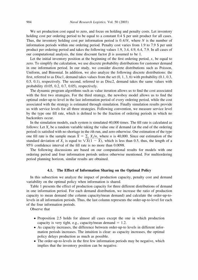
We set production cost equal to zero, and focus on holding and penalty costs. Let inventoryholding cost per ordering period to be equal to a constant 0.4 $ per unit product for all cases.Thus, the inventory holding cost per information period is 0.4/N, where N is the number ofinformation periods within one ordering period. Penalty cost varies from 1.9 to 7.9 $ per unitproduct per ordering period and takes the following values 1.9, 3.4, 4.9, 6.4, 7.9. In all cases ofour computational analysis, the time discount factor � is assumed to be 1.

Let the initial inventory position at the beginning of the first ordering period, x, be equal tozero. To simplify the calculation, we use discrete probability distributions for customer demandin one information period. In our study, we consider discrete distributions such as Poisson,Uniform, and Binomial. In addition, we also analyze the following discrete distributions: thefirst, referred to as Disc1, demand takes values from the set (0, 1, 3, 6) with probability (0.1, 0.3,0.5, 0.1), respectively. The second, referred to as Disc2, demand takes the same values withprobability (0.05, 0.2, 0.7, 0.05), respectively.

The dynamic program algorithms such as value iteration allows us to find the cost associatedwith the first two strategies. For the third strategy, the newsboy model allows us to find theoptimal order-up-to level in the last information period of every ordering period, while the costassociated with the strategy is estimated through simulation. Finally simulation results provideus with service levels for all three strategies. Following convention, we measure service levelby the type one fill rate, which is defined to be the fraction of ordering periods in which nobackorders occur.

In the simulation models, each system is simulated 40,000 times. The fill rate is calculated asfollows: Let Xi be a random variable taking the value one if demand (at the end of the orderingperiod) is satisfied with no shortage in the ith run, and zero otherwise. Our estimation of the typeone fill rate is the sample mean X� � ¥i Xi/n, where n is 40,000. Since our estimation of thestandard deviation of Xi is equal to �X� (1 � X� ), which is less than 0.5, thus, the length of a95% confidence interval of the fill rate is no more than 0.0098.

The following discussions are based on our computational results for models with oneordering period and four information periods unless otherwise mentioned. For multiorderingperiod planning horizon, similar results are obtained.

4.1. The Effect of Information Sharing on the Optimal Policy

In this subsection we analyze the impact of production capacity, penalty cost and demandvariability on the optimal policy when information is shared.

Table 1 presents the effect of production capacity for three different distributions of demandin one information period. For each demand distribution, we increase the ratio of productioncapacity to mean demand (the column capacity/mean demand) and calculate the order-up-to-levels in all information periods. Thus, the last column represents the order-up-to-level for eachof the four information periods.

Observe that

● Proposition 2.5 holds for almost all cases except the one in which productioncapacity is very tight, e.g., capacity/mean demand � 1.2.

● As capacity increases, the difference between order-up-to levels in different infor-mation periods increases. The intuition is clear: as capacity increases, the optimalpolicy delays production as much as possible.

● The order-up-to-levels in the first few information periods may be negative, whichimplies that the inventory position can be negative.


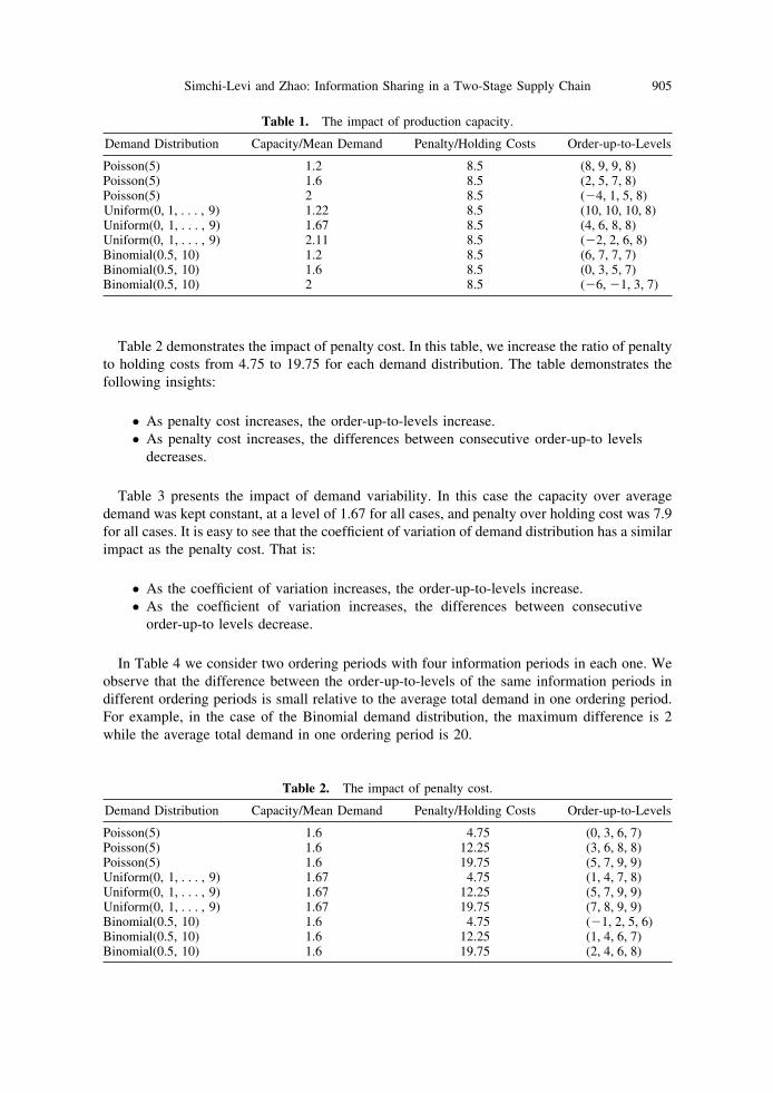
Table 2 demonstrates the impact of penalty cost. In this table, we increase the ratio of penaltyto holding costs from 4.75 to 19.75 for each demand distribution. The table demonstrates thefollowing insights:

● As penalty cost increases, the order-up-to-levels increase.● As penalty cost increases, the differences between consecutive order-up-to levels

decreases.

Table 3 presents the impact of demand variability. In this case the capacity over averagedemand was kept constant, at a level of 1.67 for all cases, and penalty over holding cost was 7.9for all cases. It is easy to see that the coefficient of variation of demand distribution has a similarimpact as the penalty cost. That is:

● As the coefficient of variation increases, the order-up-to-levels increase.● As the coefficient of variation increases, the differences between consecutive

order-up-to levels decrease.

In Table 4 we consider two ordering periods with four information periods in each one. Weobserve that the difference between the order-up-to-levels of the same information periods indifferent ordering periods is small relative to the average total demand in one ordering period.For example, in the case of the Binomial demand distribution, the maximum difference is 2while the average total demand in one ordering period is 20.

Table 1. The impact of production capacity.

Demand Distribution Capacity/Mean Demand Penalty/Holding Costs Order-up-to-Levels

Poisson(5) 1.2 8.5 (8, 9, 9, 8)Poisson(5) 1.6 8.5 (2, 5, 7, 8)Poisson(5) 2 8.5 (�4, 1, 5, 8)Uniform(0, 1, . . . , 9) 1.22 8.5 (10, 10, 10, 8)Uniform(0, 1, . . . , 9) 1.67 8.5 (4, 6, 8, 8)Uniform(0, 1, . . . , 9) 2.11 8.5 (�2, 2, 6, 8)Binomial(0.5, 10) 1.2 8.5 (6, 7, 7, 7)Binomial(0.5, 10) 1.6 8.5 (0, 3, 5, 7)Binomial(0.5, 10) 2 8.5 (�6, �1, 3, 7)

Table 2. The impact of penalty cost.


Poisson(5) 1.6 4.75 (0, 3, 6, 7)Poisson(5) 1.6 12.25 (3, 6, 8, 8)Poisson(5) 1.6 19.75 (5, 7, 9, 9)Uniform(0, 1, . . . , 9) 1.67 4.75 (1, 4, 7, 8)Uniform(0, 1, . . . , 9) 1.67 12.25 (5, 7, 9, 9)Uniform(0, 1, . . . , 9) 1.67 19.75 (7, 8, 9, 9)Binomial(0.5, 10) 1.6 4.75 (�1, 2, 5, 6)Binomial(0.5, 10) 1.6 12.25 (1, 4, 6, 7)Binomial(0.5, 10) 1.6 19.75 (2, 4, 6, 8)


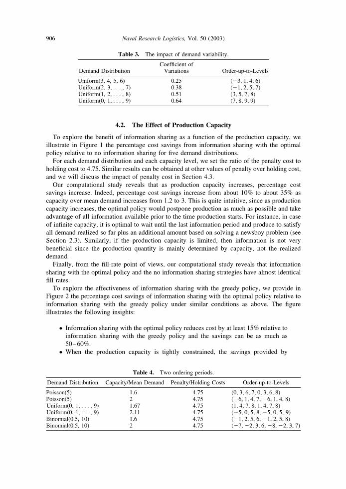
4.2. The Effect of Production Capacity

To explore the benefit of information sharing as a function of the production capacity, weillustrate in Figure 1 the percentage cost savings from information sharing with the optimalpolicy relative to no information sharing for five demand distributions.

For each demand distribution and each capacity level, we set the ratio of the penalty cost toholding cost to 4.75. Similar results can be obtained at other values of penalty over holding cost,and we will discuss the impact of penalty cost in Section 4.3.

Our computational study reveals that as production capacity increases, percentage costsavings increase. Indeed, percentage cost savings increase from about 10% to about 35% ascapacity over mean demand increases from 1.2 to 3. This is quite intuitive, since as productioncapacity increases, the optimal policy would postpone production as much as possible and takeadvantage of all information available prior to the time production starts. For instance, in caseof infinite capacity, it is optimal to wait until the last information period and produce to satisfyall demand realized so far plus an additional amount based on solving a newsboy problem (seeSection 2.3). Similarly, if the production capacity is limited, then information is not verybeneficial since the production quantity is mainly determined by capacity, not the realizeddemand.

Finally, from the fill-rate point of views, our computational study reveals that informationsharing with the optimal policy and the no information sharing strategies have almost identicalfill rates.

To explore the effectiveness of information sharing with the greedy policy, we provide inFigure 2 the percentage cost savings of information sharing with the optimal policy relative toinformation sharing with the greedy policy under similar conditions as above. The figureillustrates the following insights:

● Information sharing with the optimal policy reduces cost by at least 15% relative toinformation sharing with the greedy policy and the savings can be as much as50–60%.

● When the production capacity is tightly constrained, the savings provided by

Table 3. The impact of demand variability.

Demand DistributionCoefficient of

Variations Order-up-to-Levels

Uniform(3, 4, 5, 6) 0.25 (�3, 1, 4, 6)Uniform(2, 3, . . . , 7) 0.38 (�1, 2, 5, 7)Uniform(1, 2, . . . , 8) 0.51 (3, 5, 7, 8)Uniform(0, 1, . . . , 9) 0.64 (7, 8, 9, 9)

Table 4. Two ordering periods.


Poisson(5) 1.6 4.75 (0, 3, 6, 7, 0, 3, 6, 8)Poisson(5) 2 4.75 (�6, 1, 4, 7, �6, 1, 4, 8)Uniform(0, 1, . . . , 9) 1.67 4.75 (1, 4, 7, 8, 1, 4, 7, 8)Uniform(0, 1, . . . , 9) 2.11 4.75 (�5, 0, 5, 8, �5, 0, 5, 9)Binomial(0.5, 10) 1.6 4.75 (�1, 2, 5, 6, �1, 2, 5, 8)Binomial(0.5, 10) 2 4.75 (�7, �2, 3, 6, �8, �2, 3, 7)


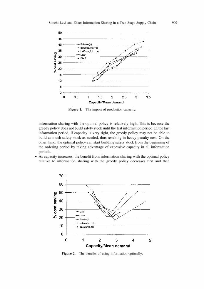
information sharing with the optimal policy is relatively high. This is because thegreedy policy does not build safety stock until the last information period. In the lastinformation period, if capacity is very tight, the greedy policy may not be able tobuild as much safety stock as needed, thus resulting in heavy penalty cost. On theother hand, the optimal policy can start building safety stock from the beginning ofthe ordering period by taking advantage of excessive capacity in all informationperiods.

● As capacity increases, the benefit from information sharing with the optimal policyrelative to information sharing with the greedy policy decreases first and then

Figure 1. The impact of production capacity.

Figure 2. The benefits of using information optimally.


increases again. This is true, since as capacity becomes very large relative toaverage demand, information sharing with the optimal policy will postpone pro-duction as much as possible, while information sharing with the greedy policy willbuild inventory starting from the beginning of ordering periods, thus resulting inheavy inventory holding cost.

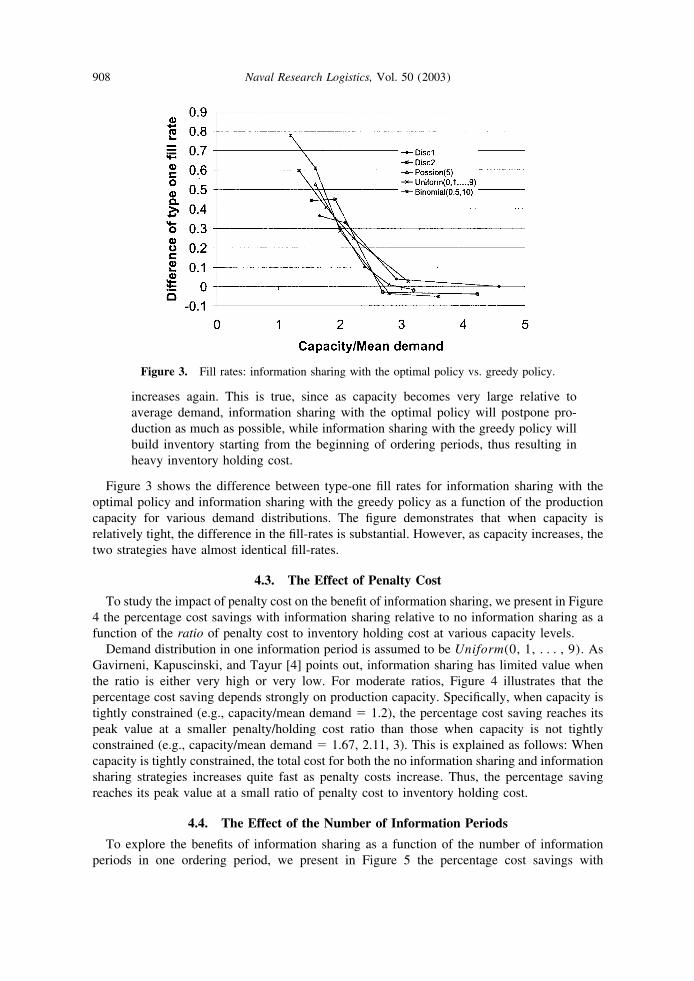
Figure 3 shows the difference between type-one fill rates for information sharing with theoptimal policy and information sharing with the greedy policy as a function of the productioncapacity for various demand distributions. The figure demonstrates that when capacity isrelatively tight, the difference in the fill-rates is substantial. However, as capacity increases, thetwo strategies have almost identical fill-rates.

4.3. The Effect of Penalty Cost

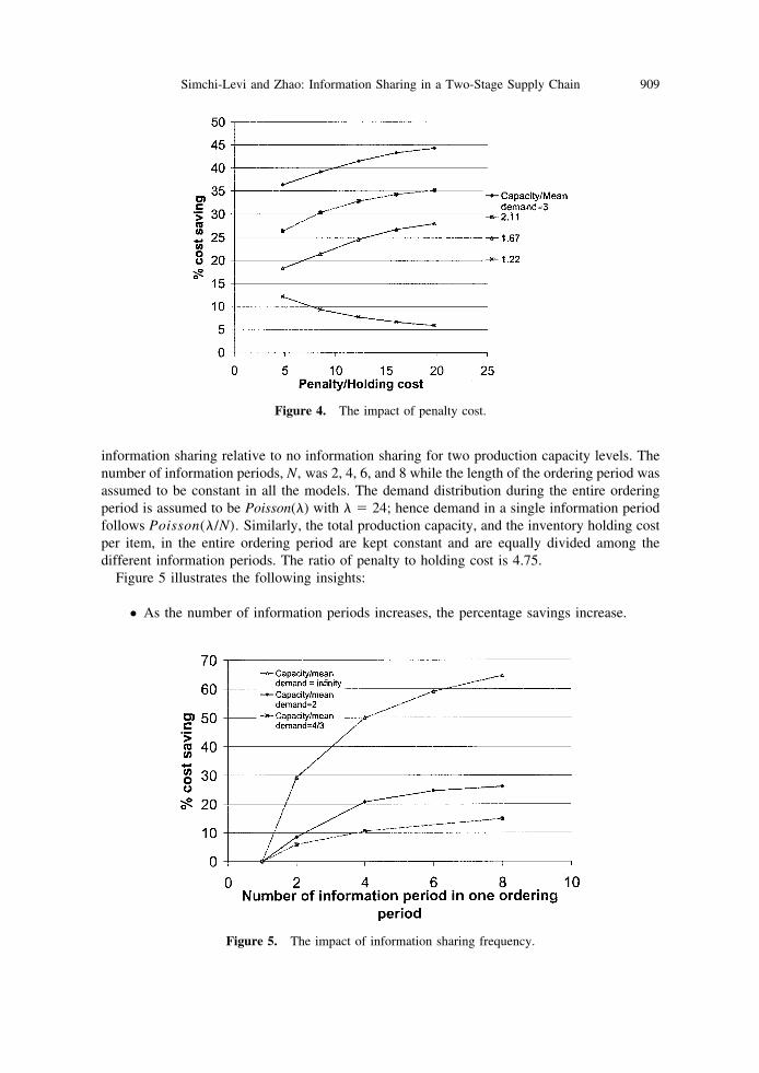
To study the impact of penalty cost on the benefit of information sharing, we present in Figure4 the percentage cost savings with information sharing relative to no information sharing as afunction of the ratio of penalty cost to inventory holding cost at various capacity levels.

Demand distribution in one information period is assumed to be Uniform(0, 1, . . . , 9). AsGavirneni, Kapuscinski, and Tayur [4] points out, information sharing has limited value whenthe ratio is either very high or very low. For moderate ratios, Figure 4 illustrates that thepercentage cost saving depends strongly on production capacity. Specifically, when capacity istightly constrained (e.g., capacity/mean demand � 1.2), the percentage cost saving reaches itspeak value at a smaller penalty/holding cost ratio than those when capacity is not tightlyconstrained (e.g., capacity/mean demand � 1.67, 2.11, 3). This is explained as follows: Whencapacity is tightly constrained, the total cost for both the no information sharing and informationsharing strategies increases quite fast as penalty costs increase. Thus, the percentage savingreaches its peak value at a small ratio of penalty cost to inventory holding cost.

4.4. The Effect of the Number of Information Periods

To explore the benefits of information sharing as a function of the number of informationperiods in one ordering period, we present in Figure 5 the percentage cost savings with

Figure 3. Fill rates: information sharing with the optimal policy vs. greedy policy.


information sharing relative to no information sharing for two production capacity levels. Thenumber of information periods, N, was 2, 4, 6, and 8 while the length of the ordering period wasassumed to be constant in all the models. The demand distribution during the entire orderingperiod is assumed to be Poisson(�) with � � 24; hence demand in a single information periodfollows Poisson(�/N). Similarly, the total production capacity, and the inventory holding costper item, in the entire ordering period are kept constant and are equally divided among thedifferent information periods. The ratio of penalty to holding cost is 4.75.

Figure 5 illustrates the following insights:

● As the number of information periods increases, the percentage savings increase.

Figure 4. The impact of penalty cost.

Figure 5. The impact of information sharing frequency.


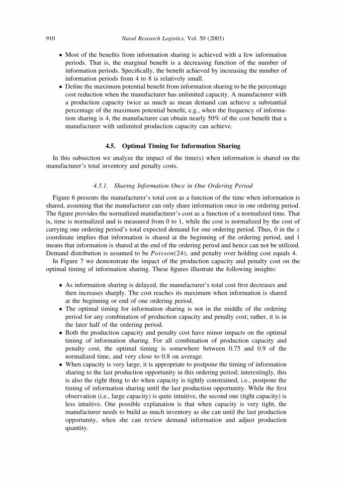
● Most of the benefits from information sharing is achieved with a few informationperiods. That is, the marginal benefit is a decreasing function of the number ofinformation periods. Specifically, the benefit achieved by increasing the number ofinformation periods from 4 to 8 is relatively small.

● Define the maximum potential benefit from information sharing to be the percentagecost reduction when the manufacturer has unlimited capacity. A manufacturer witha production capacity twice as much as mean demand can achieve a substantialpercentage of the maximum potential benefit, e.g., when the frequency of informa-tion sharing is 4, the manufacturer can obtain nearly 50% of the cost benefit that amanufacturer with unlimited production capacity can achieve.

4.5. Optimal Timing for Information Sharing

In this subsection we analyze the impact of the time(s) when information is shared on themanufacturer’s total inventory and penalty costs.

4.5.1. Sharing Information Once in One Ordering Period

Figure 6 presents the manufacturer’s total cost as a function of the time when information isshared, assuming that the manufacturer can only share information once in one ordering period.The figure provides the normalized manufacturer’s cost as a function of a normalized time. Thatis, time is normalized and is measured from 0 to 1, while the cost is normalized by the cost ofcarrying one ordering period’s total expected demand for one ordering period. Thus, 0 in the xcoordinate implies that information is shared at the beginning of the ordering period, and 1means that information is shared at the end of the ordering period and hence can not be utilized.Demand distribution is assumed to be Poisson(24), and penalty over holding cost equals 4.

In Figure 7 we demonstrate the impact of the production capacity and penalty cost on theoptimal timing of information sharing. These figures illustrate the following insights:

● As information sharing is delayed, the manufacturer’s total cost first decreases andthen increases sharply. The cost reaches its maximum when information is sharedat the beginning or end of one ordering period.

● The optimal timing for information sharing is not in the middle of the orderingperiod for any combination of production capacity and penalty cost; rather, it is inthe later half of the ordering period.

● Both the production capacity and penalty cost have minor impacts on the optimaltiming of information sharing. For all combination of production capacity andpenalty cost, the optimal timing is somewhere between 0.75 and 0.9 of thenormalized time, and very close to 0.8 on average.

● When capacity is very large, it is appropriate to postpone the timing of informationsharing to the last production opportunity in this ordering period; interestingly, thisis also the right thing to do when capacity is tightly constrained, i.e., postpone thetiming of information sharing until the last production opportunity. While the firstobservation (i.e., large capacity) is quite intuitive, the second one (tight capacity) isless intuitive. One possible explanation is that when capacity is very tight, themanufacturer needs to build as much inventory as she can until the last productionopportunity, when she can review demand information and adjust productionquantity.


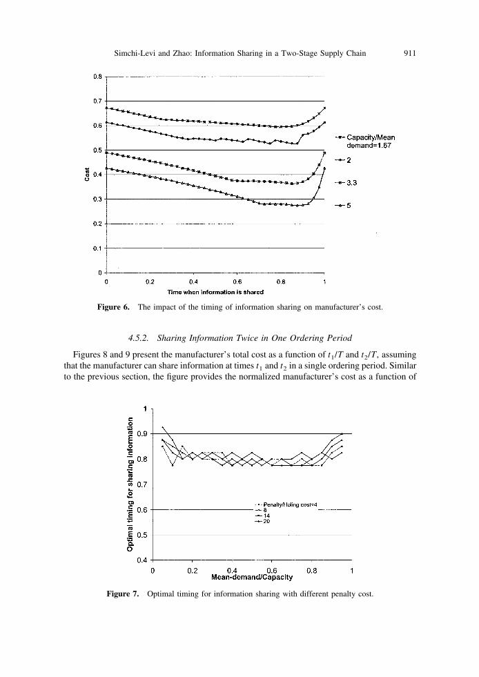
4.5.2. Sharing Information Twice in One Ordering Period

Figures 8 and 9 present the manufacturer’s total cost as a function of t1/T and t2/T, assumingthat the manufacturer can share information at times t1 and t2 in a single ordering period. Similarto the previous section, the figure provides the normalized manufacturer’s cost as a function of

Figure 6. The impact of the timing of information sharing on manufacturer’s cost.

Figure 7. Optimal timing for information sharing with different penalty cost.


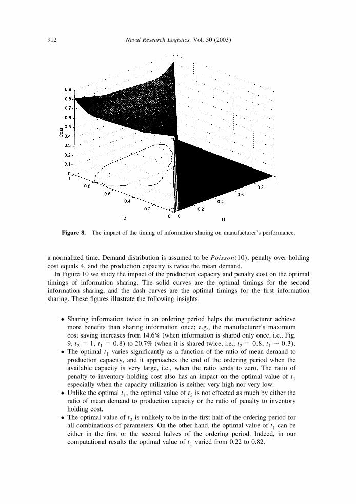
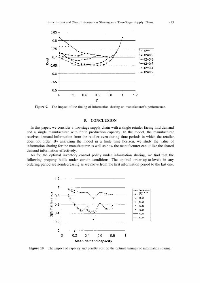
a normalized time. Demand distribution is assumed to be Poisson(10), penalty over holdingcost equals 4, and the production capacity is twice the mean demand.

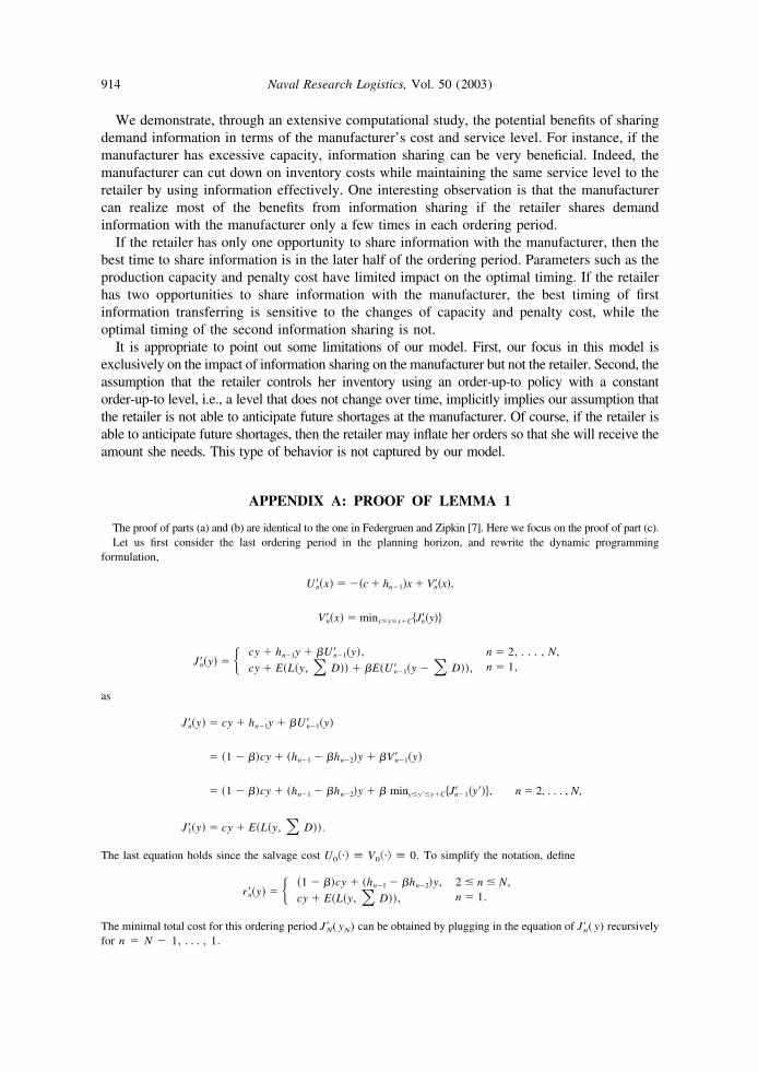
In Figure 10 we study the impact of the production capacity and penalty cost on the optimaltimings of information sharing. The solid curves are the optimal timings for the secondinformation sharing, and the dash curves are the optimal timings for the first informationsharing. These figures illustrate the following insights:

● Sharing information twice in an ordering period helps the manufacturer achievemore benefits than sharing information once; e.g., the manufacturer’s maximumcost saving increases from 14.6% (when information is shared only once, i.e., Fig.9, t2 � 1, t1 � 0.8) to 20.7% (when it is shared twice, i.e., t2 � 0.8, t1 � 0.3).

● The optimal t1 varies significantly as a function of the ratio of mean demand toproduction capacity, and it approaches the end of the ordering period when theavailable capacity is very large, i.e., when the ratio tends to zero. The ratio ofpenalty to inventory holding cost also has an impact on the optimal value of t1

especially when the capacity utilization is neither very high nor very low.● Unlike the optimal t1, the optimal value of t2 is not effected as much by either the

ratio of mean demand to production capacity or the ratio of penalty to inventoryholding cost.

● The optimal value of t2 is unlikely to be in the first half of the ordering period forall combinations of parameters. On the other hand, the optimal value of t1 can beeither in the first or the second halves of the ordering period. Indeed, in ourcomputational results the optimal value of t1 varied from 0.22 to 0.82.

Figure 8. The impact of the timing of information sharing on manufacturer’s performance.


5. CONCLUSION

In this paper, we consider a two-stage supply chain with a single retailer facing i.i.d demandand a single manufacturer with finite production capacity. In the model, the manufacturerreceives demand information from the retailer even during time periods in which the retailerdoes not order. By analyzing the model in a finite time horizon, we study the value ofinformation sharing for the manufacturer as well as how the manufacturer can utilize the shareddemand information effectively.

As for the optimal inventory control policy under information sharing, we find that thefollowing property holds under certain conditions: The optimal order-up-to-levels in anyordering period are nondecreasing as we move from the first information period to the last one.

Figure 9. The impact of the timing of information sharing on manufacturer’s performance.

Figure 10. The impact of capacity and penalty cost on the optimal timings of information sharing.


We demonstrate, through an extensive computational study, the potential benefits of sharingdemand information in terms of the manufacturer’s cost and service level. For instance, if themanufacturer has excessive capacity, information sharing can be very beneficial. Indeed, themanufacturer can cut down on inventory costs while maintaining the same service level to theretailer by using information effectively. One interesting observation is that the manufacturercan realize most of the benefits from information sharing if the retailer shares demandinformation with the manufacturer only a few times in each ordering period.

If the retailer has only one opportunity to share information with the manufacturer, then thebest time to share information is in the later half of the ordering period. Parameters such as theproduction capacity and penalty cost have limited impact on the optimal timing. If the retailerhas two opportunities to share information with the manufacturer, the best timing of firstinformation transferring is sensitive to the changes of capacity and penalty cost, while theoptimal timing of the second information sharing is not.

It is appropriate to point out some limitations of our model. First, our focus in this model isexclusively on the impact of information sharing on the manufacturer but not the retailer. Second, theassumption that the retailer controls her inventory using an order-up-to policy with a constantorder-up-to level, i.e., a level that does not change over time, implicitly implies our assumption thatthe retailer is not able to anticipate future shortages at the manufacturer. Of course, if the retailer isable to anticipate future shortages, then the retailer may inflate her orders so that she will receive theamount she needs. This type of behavior is not captured by our model.

APPENDIX A: PROOF OF LEMMA 1

The proof of parts (a) and (b) are identical to the one in Federgruen and Zipkin [7]. Here we focus on the proof of part (c).Let us first consider the last ordering period in the planning horizon, and rewrite the dynamic programming

formulation,

U�n�x� � ��c � hn�1�x � V�n�x�,

V�n�x� � minx�y�x�CJ�n�y�

J�n�y� � � cy � hn�1y � �U�n�1�y�, n � 2, . . . , N,

cy � E�L�y, � D�� E�U�n�1�y � � D��, n � 1,

as

J�n�y� � cy � hn�1y � �U�n�1�y�

� �1 � ��cy � �hn�1 � �hn�2�y � �V�n�1�y�

� �1 � ��cy � �hn�1 � �hn�2�y � � miny�y��y�CJ�n�1�y��, n � 2, . . . , N,

J�1�y� � cy � E�L�y, � D��.

The last equation holds since the salvage cost U0� � V0� � 0. To simplify the notation, define

r�n�y� � � �1 � ��cy � �hn�1 � �hn�2�y, 2 � n � N,

cy � E�L�y, � D��, n � 1.

The minimal total cost for this ordering period J�N( yN) can be obtained by plugging in the equation of J�n( y) recursivelyfor n � N � 1, . . . , 1.


J�N�yN� � r�N�yN� � � minyN�yN�1�yN�Cr�N�1�yN�1� � · · · � � miny3�y2�y3�Cr�2�y2� � � miny2�y1�y2�Cr�1�y1�· · ·.

(7)

Notice that for all n � N, N � 1, . . . , 1, if y � �n minimizes r�n( y�) in interval [ y, y � C], then

�miny�y��y�Cr�n�y�� r�n�y�� r�n�y � �n� � r�n�y�� n�,

since r�n( y) is at most proportional to a linear function of y. Because �n � C, the absolute difference between (7) and¥n�1

N �N�n r�n( yN) is bounded by a finite number, which is independent of y. Finally, expanding ¥n�1N �N�n r�n( y),

we obtain ¥n�1N �N�n r�n( y) � cy � hN�1y � �N�1E(L( y, ¥ D)). Hence, in order for Jn( y) 3 �� for all n when

y 3 ��, we need �N�1� � c � hN�1.The proof for other ordering periods is similar. �

APPENDIX B: PROOF OF PART (c) OF LEMMA 3

The case when y 3 �� is straightforward. Thus, we only need to show that if �N�1� � c � hN�1, then Jn( y)3 �� for all n � N, N � 1, . . . , 1 when y 3 ��.

For this purpose, let us consider the last ordering period in the planning horizon. From Eq. (4),

Jn�y� � �n�y� � �E�Un�1�y � D��

� rn�y� � �E�Vn�1�y � D��

� rn�y� � �E�miny�D�y��y�D�CJn�1�y��, 2, . . . , N

J1�y� � r1�y�,

where the salvage cost U0� � V0� � 0, and

rn�y� � � �1 � ��cy � �hn�1 � �hn�2�y � ��c � hn�2��, 2 � n � N,cy � E�L�y, D��, n � 1.

The minimal total cost for this ordering period JN( yN) can be obtained by plugging in the equation of Jn( y) recursivelyfor n � N � 1, . . . , 1.

JN�yN� � rN�yN� � �E�minyN�D�yN�1�yN�D�CrN�1�yN�1� � · · · � �E�miny2�D�y1�y2�D�Cr1�y1��· · ·�. (8)

Similarly to Appendix A, we observe that for all n � N, N � 1, . . . , 1,

�E�miny�D�y��y�D�Crn�y�� rn�y�� E�rn�y � �n�D�� rn�y��,

with D � C � �n(D) � D, and

�E�rn�y � �n�D�� rn�y��

��

rn�y � �n�D�� rn�y��fD�D� dD�

��

��

�n�D�fD�D� dD� ,

since rn( y) is at most proportional to a linear function of y. Because �� n(D) fD(D) dD� � max{�� C�, ��},

the absolute difference between (8) and ¥n�1N �N�n rn( yN) is bounded by a finite number, which is independent of y.

Finally, expanding ¥n�1N �N�n rn( yN) we obtain ¥n�1

N �N�n rn( y) � cy � hN�1y � �N�1E(L( y, D)) � constant.Hence, in order to have Jn( y) 3 �� for all n when y 3 ��, we need �N�1� � c � hN�1.

The proof for other ordering periods is similar. �


ACKNOWLEDGMENTS

Research was supported in part by ONR Contracts N00014-95-1-0232 and N00014-01-1-0146, and by NSF Contracts DDM-9322828 and DMI-9732795.

REFERENCES

[1] Y. Aviv and A. Federgruen, The operational benefits of information sharing and vendor managedinventory (VMI) programs, Working Paper, Washington University, St. Louis, MO, 1998.

[2] G.P. Cachon and M. Fisher, Supply chain inventory management and the value of shared information,Management Sci 46 (2000), 1032–1050.

[3] A. Federgruen and P. Zipkin, An inventory model with limited production capacity and uncertaindemands 2: The discounted-cost criterion, Math Oper Res 11 (1986), 208–215.

[4] S. Gavirneni, R. Kapuscinski, and S. Tayur, Value of information in capacitated supply chains,Management Sci 45 (1999), 16–24.

[5] G. Hadley and T.M. Whitin, Analysis of inventory systems. Prentice-Hall, Englewood Cliffs, NJ,1963.

[6] D. Heyman and M. Sobel, Stochastic models in operations research, McGraw-Hill, New York, 1984,Vol. 2.

[7] H.L. Lee and S. Nahmias, “Single-product, single-location models,” Handbooks in operations researchand management science, North-Holland, Amsterdam, 1993, Vol. 4.

[8] D. Simchi-Levi, F. Kaminsky, and E. Simchi-Levi, Designing and managing the supply chain,Irwin/McGraw-Hill, Chicago, IL, 1999.

[9] T. Stein and J. Sweat, Killer supply chains, Inform Week (1998), http://www.informationweek.com/708/08iukil.htm.


the value of information sharing in a two-stage supply...

Documents