the use of single foraminiferal shells for recording ... · the use of single foraminiferal shells...
TRANSCRIPT
The use of single foraminiferal shells for recording
seasonal temperatures and water column stratification and
its applicability to the fossil record
Dissertation zur Erlangung des akademischen Grades eines Doktors der
Naturwissenschaften
Dr. rer. nat.
am Fachbereich 5 (Geowissenschaften) der Universität Bremen
Tim Haarmann
Bremen, 2012

Gutachter der Dissertation:
Prof. Dr. Gerold Wefer
Prof. Dr. Geert-Jan Brummer
Tag des Dissertationskolloquiums:
19. Dezember 2012 um 16 Uhr c.t. im MARUM, Raum 2070


ERKLÄRUNG
Name: Tim Haarmann Datum: 02. April 2012
Anschrift: Moselstraße 18, 28199 Bremen
-----------------------------------------------------------------------------------------------------------------
Hiermit versichere ich an Eides statt, dass ich
1. Die Arbeit ohne unerlaubte fremde Hilfe angefertigt habe
2. keine anderen als die von mir angegebenen Quellen und Hilfsmittel benutzt habe und
3. die den benutzten Werken wörtlich oder inhaltlich entnommenen Stellen als solche
kenntlich gemacht habe
-----------------------------------------------------------------------------------------------------------------
Bremen, 02. April 2012
Tim Haarmann
(Unterschrift)

ACKNOWLEDGEMENTS
First of all, I wish to thank Prof. Dr. Gerold Wefer and Dr. Torsten Bickert who gave me
the chance to carry out this PhD project. They have constantly been interested in the
progress of my PhD project and shared their great scientific knowledge with me. They
encouraged me to participate in several conferences, from which I benefited a lot. I am
very grateful to Torsten for always taking the time for discussions and advice.
A great thank you goes to my co-supervisor Dr. Gerald Ganssen, head of the cluster Earth
& Climate at the Faculty of Earth Sciences of the Vrije Universiteit Amsterdam. During
my abroad stay in Amsterdam, Gerald and Dr. Frank Peeters took a lot of time for
discussions and advice and introduced me to the analysis of oxygen isotopes from single
foraminiferal shells. For her laboratory assistance during my time in Amsterdam, I wish
to thank Suzanne Verdegaal a lot.
It is almost impossible to thank all the people that helped me in the daily work and who
shared their expertise with me during these years. I am especially grateful to Dr. Ed
Hathorne, who introduced me into the Marum flow-through cleaning device and who was
a great help in tackling all problems that had to be overcome in order to get the system
properly running. For their technical support, I acknowledge Matthias Lange and
Wolfgang Schunn. Dr. Mahyar Mohtadi, Dr. Jeroen Groeneveld and Dr. Stephan Steinke
took a lot of time for discussions, assisted me with writing and introduced me into many
aspects of foraminiferal analysis. Their help was absolutely priceless. For laboratory
assistance, I want to express my gratitude to Heike Anders and Petra Witte.
My family, friends and office mates have constantly encouraged me during these years. I
especially want to thank Anna Kloss, Francesca Vallé and Rony Küchler for the great
time in the office.
I thank the Center for Marine Environmental Sciences (MARUM) for the sample
collection and technical support. The Deutsche Forschungsgemeinschaft (DFG) is
gratefully acknowledged for supporting me with a scholarship within the International
Graduate College EUROPROX. For organizing regular EUROPROX “coffee & science”
meetings, I wish to thank Dr. Dorothee Wilhelms-Dick and Dr. Cletus Itambi.

ABSTRACT
Mg/Ca- and oxygen isotope ratios in the shells of planktic foraminifera are widely used in
paleoceanographic studies for the reconstruction of water temperatures. Standard
investigations analyze multiple shells of a species at once. However, when single shells
are analyzed, substantial differences of the Mg/Ca- and oxygen isotope ratios are found.
These are explained by seasonality and natural variability, and are increasingly used for
the reconstruction of past environmental conditions. The present thesis analyzes the
differences of the Mg/Ca- and oxygen isotope ratios between individual shells in the
upwelling region off Northwest-Africa. The aim of this thesis is to quantify natural
variability, to improve the applicability of single shells for the reconstruction of
temperature seasonality and to show the potential of single specimens for recording past
ocean stratification.
In the present thesis, calcification temperatures are calculated from the Mg/Ca ratios in
single shells of the surface-dwelling planktic foraminifera Globigerinoides ruber (pink),
Globigerinoides ruber (white) and the deep-dwelling species Globorotalia inflata,
collected from a sediment trap off Northwest-Africa at 20°45.6’N, 18°41.9’W
(Manuscript I). Single shells of G. ruber (pink) showed substantially different Mg/Ca
temperatures linked to the seasonal temperature cycle at the sea surface, whereas the
Mg/Ca temperatures from G. ruber (white) did not. Mg/Ca temperatures from single
shells of G. inflata did not show seasonal differences and correspond to water depths
between the sea surface and about 400 m. Changes in the Mg/Ca range are significant
when they are larger than 0.80 mmol/mol (G. ruber (pink)) or 0.34 mmol/mol (G. inflata).
For G. ruber (pink), this corresponds to a change in the temperature amplitude of >4°C
and >1.7°C for G. inflata.
In order to verify the calculated temperature amplitudes and to test them for their
paleoceanographic applicability, these were compared to single specimen calcification
temperature ranges of G. inflata, for selected time slices throughout the past 22,000 years
in the study area (Manuscript II). The temperature range reconstructed from near present
(570 years before present) samples is in good agreement with the one reconstructed from
the sediment trap samples. However, in samples from the last deglaciation, the range was
significantly reduced. Comparison to water temperatures predicted by a climate model
suggests that the reduction is due to a stronger thermal stratification off Northwest-Africa
during the deglaciation and a smaller depth habitat range of G. inflata.
Previous studies found high sea surface temperatures in the study area during the Last
Glacial Maximum (23,000 - 19,000 years before present), which were explained by
weaker upwelling of deeper, colder subsurface water. In this thesis, upwelling strength
and water temperatures at the sea surface and ~150 m water depth were reconstructed for
the past 24,000 years, using the relative abundance of Globigerina bulloides and Mg/Ca
analyses of G. ruber (pink), G. bulloides and G. inflata (Manuscript III). The results
contradict previous assumptions and suggest high upwelling intensities between 24,000
and 16,000 years before present. Further, a high Mg/Ca temperature variability of the
surface dwelling species G. ruber (pink) and G. bulloides was found, in contrast to the
subsurface dwelling species G. inflata. An inspection of daily satellite data between 1982
and 2008 shows a high degree of temperature variability in the study area and high
temperatures, likely through the advection of warm surface waters during times of high
wind strength. It is presumed that in the past this mechanism might have also caused
higher SSTs at the study site during generally cold climatic states.
ZUSAMMENFASSUNG
Mg/Ca- und Sauerstoffisotopenverhältnisse in Schalen planktischer Foraminiferen werden
in vielen paläozeanographischen Studien zur Rekonstruktion von Wassertemperaturen
verwendet. Bei der herkömmlichen Methode werden mehrere Schalen einer Art
gleichzeitig analysiert. Werden jedoch einzelne Schalen analysiert zeigt sich, dass
erhebliche Unterschiede in Mg/Ca- und Sauerstoffisotopenverhältnissen einzelner
Individuen bestehen. Diese werden durch Saisonalität und natürliche Variabilität erklärt
und zunehmend zur Rekonstruktion vergangener Umweltbedingungen genutzt. Die
vorliegende Arbeit erfasst die Unterschiede der Mg/Ca- und
Sauerstoffisotopenverhältnisse zwischen einzelnen Individuen planktischer Foraminiferen
im Auftriebsgebiet vor Nordwest-Afrika. Ziel der Arbeit ist es, natürliche Variabilität zu
quantifizieren, die Nutzbarkeit von Einzelschalen für die Rekonstruktion von
Temperatursaisonalität zu verbessern und die Anwendbarkeit von Einzelschalen für die
Rekonstruktion der thermischen Ozeanstratifizierung aufzuzeigen.
In der vorliegenden Arbeit werden Kalzifizierungstemperaturen aus den Mg/Ca
Verhältnissen in Einzelschalen der an der Wasseroberfläche lebenden planktischen
Foraminiferenarten Globigerinoides ruber (pink), Globigerinoides ruber (white) und der
tieflebenden Art Globorotalia inflata berechnet, welche in einer Sedimentfalle vor
Nordwest-Afrika (20°45.6’N, 18°41.9’W) gesammelt wurden (Manuskript I).
Einzelschalen von G. ruber (pink) wiesen deutlich unterschiedliche Mg/Ca-Temperaturen
auf, welche dem saisonalen Temperaturverlauf an der Wasseroberfläche folgten,
wohingegen die Mg/Ca-Temperaturen von G. ruber (white) keinen Zusammenhang mit
saisonalen Wasseroberflächentemperaturen zeigten. Mg/Ca-Temperaturen in
Einzelschalen von G. inflata zeigten keine saisonalen Unterschiede und entsprachen
Wassertemperaturen zwischen der Meeresoberfläche und etwa 400 m Wassertiefe.
Änderungen in der Mg/Ca Spannbreite zwischen einzelnen Individuen sind dann
signifikant, wenn sie 0,80 mmol/mol (G. ruber (pink)) bzw. 0,34 mmol/mol (G. inflata)
überschreiten. Im Fall von G. ruber (pink) entspricht dies einer Temperaturschwankung
von >4°C und im Fall von G. inflata von >1,7°C.
Um die zuvor berechneten Temperaturspannen zu verifizieren und auf ihre
paläozeanographische Anwendbarkeit hin zu überprüfen wurden diese für G. inflata mit
rekonstruierten Temperaturspannen aus ausgewählte Zeitabschnitten innerhalb der
vergangenen 22.000 Jahre im gleichen Arbeitsgebiet verglichen (Manuskript II). Es
zeigte sich, dass Proben der jüngeren Vergangenheit (570 Jahre vor heute) gut mit der in
der Sedimentfallenstudie rekonstruierten Temperaturspanne übereinstimmen. In Proben
aus der letzten Abschmelzphase war diese jedoch signifikant reduziert. Der Vergleich mit
berechneten Wassertemperaturen eines Klimamodels deutet darauf hin, dass diese
Reduktion auf eine ausgeprägtere thermische Stratifizierung vor Nordwest-Afrika und ein
schmaleres Tiefenhabitat von G. inflata während der letzten Abschmelzphase
zurückzuführen ist.
Frühere Untersuchungen erklären hohe Wasseroberflächentemperaturen im Arbeitsgebiet
während des letzten glazialen Maximums (23.000 – 19.000 Jahre vor heute) mit
geringerem Auftrieb des tieferen und kälteren Wassers. In der vorliegenden Arbeit
wurden Auftriebsintensitäten im Arbeitsgebiet und Temperaturen der letzten 24.000 Jahre
für die Wasseroberfläche und eine Wassertiefe von ~150 m anhand der relativen
Häufigkeit von Globigerina bulloides sowie Mg/Ca Analysen an G. ruber (pink),
G. bulloides und G. inflata rekonstruiert (Manuskript III). Die Ergebnisse stehen im
Widerspruch zu früheren Annahmen und weisen auf hohe Auftriebsintensität zwischen
24.000 und 16.000 Jahren vor heute hin. Zudem zeigte sich eine hohe Mg/Ca-
Temperaturvariabilität der oberflächenlebenden Arten G. ruber (pink) und G. bulloides
im Vergleich zur tieflebenden Art G. inflata. Die Auswertung täglicher Satellitendaten
zwischen 1982 und 2008 belegt eine hohe Temperaturvariabilität im Arbeitsgebiet und
deutet darauf hin, dass hohe Temperaturen im Arbeitsgebiet insbesondere in Verbindung
mit hoher Windintensität auftreten und vermutlich durch die Advektion warmen
südlichen Oberflächenwassers bedingt werden. Dieser Mechanismus könnte auch in der
Vergangenheit zum Teil hohe Wasseroberflächentemperaturen während grundsätzlich
kalter Klimazustände bedingt haben.
TABLE OF CONTENTS
I. INTRODUCTION.................................................................................................................1
1.1 Planktic foraminifera as carriers for geochemical temperature proxies ...........................1
1.2 Short-term environmental changes recorded by planktic foraminifera ............................2
1.2.1 Surface-dwelling species ...........................................................................................3
1.2.2 Subsurface-dwelling species......................................................................................7
1.3 Assessing temperature extrema ........................................................................................9
1.4 Cleaning and measurement of individual shells .............................................................10
II. THESIS OUTLINE ...........................................................................................................15
III. MATERIAL AND STUDY SITE ...................................................................................19
3.1 Samples...........................................................................................................................19
3.2 Study site ........................................................................................................................19
IV. MANUSCRIPTS ..............................................................................................................25
4.1 Manuscript 1: Mg/Ca ratios of single planktonic foraminifer shells and the potential
to reconstruct the thermal seasonality of the water column .................................................25
4.1.1 Introduction .............................................................................................................26
4.1.2 Study area ................................................................................................................29
4.1.3 Material and methods ..............................................................................................30
4.1.4 Results .....................................................................................................................34
4.1.5 Discussion................................................................................................................37
4.1.6 Conclusions .............................................................................................................46
4.2 Manuscript 2: Subsurface thermal stratification off NW Africa during the past
24,000 years – Inferences from single planktic foraminifer shells.......................................59
4.2.1 Introduction .............................................................................................................60
4.2.2 Modern climate........................................................................................................61
4.2.3 Material and methods ..............................................................................................63
4.2.4 Results .....................................................................................................................69
4.2.5 Discussion................................................................................................................71
4.2.6 Conclusions .............................................................................................................80
4.3 Manuscript 3: Upwelling strength off Cape Blanc (NW Africa) during the past
24,000 years – Effects on the surface and subsurface Mg/Ca temperature records .............85
4.3.1 Introduction .............................................................................................................86
4.3.2 Modern climate........................................................................................................87
4.3.3 Material and methods ..............................................................................................89
4.3.4 Results .....................................................................................................................94
4.3.5 Discussion................................................................................................................96
4.3.6 Conclusions ...........................................................................................................103
V. SUMMARY AND OUTLOOK.......................................................................................109
VI. REFERENCES ...............................................................................................................117
Planktic foraminifera – Carriers for temperature proxies INTRODUCTION
1
I. INTRODUCTION
1.1 Planktic foraminifera as carriers for geochemical temperature proxies
Planktic foraminifera are short-lived heterotrophic protists that live in the marine upper
ocean environment. In their adult stage, their shells range in sizes between 100 µm and
2 mm formed of calcium carbonate precipitated from the seawater carbonate. They either
live in the shallow mixed layer or in the subsurface water column close to or below the
thermocline. About fifty species are known [Kucera, 2007] that occur in all oceans from
the tropics to the high latitudes and from surface waters to water depths of several
hundred meters [e.g.; Fairbanks et al., 1982]. Each species has different ecological and
temperature preferences that determine their geographical distribution, their seasonal
succession, and their vertical distribution in the water column [e.g.; Žari et al., 2005].
Temperature information can be extracted from the chemical composition of their
calcitic shells, given that these were precipitated in equilibrium with the ambient
seawater. The classical approach stems from the work of Cesare Emiliani [1955], who
used the foraminiferal shell stable oxygen isotopic composition ( 18Oc) to deduce
Pleistocene sea surface temperatures (SST). The use of foraminiferal oxygen isotopes as a
paleothermometer is based on the ratio of the heavy (18O) to the light (16O) isotope in
their shells, which is a function of both, temperature and the 18O of the ambient seawater
( 18Ow), from which the shells are precipitated. As has been shown in the following
decades, variability of 18Ow substantially influences the use of oxygen isotopes in
foraminiferal calcite for determining temperatures. During cold periods within the
Pleistocene for instance, the ocean was enriched by ~1.2 to 1.5 ‰, as a result of the
preferential removal of 16O during evaporation from the sea surface and its storage on the
continental ice sheets, also termed as ice-volume effect [e.g.; Shackleton, 1967].
Likewise, locally differing evaporation rates change the 18Ow, thereby impairing the
accuracy of the oxygen isotope thermometer.
In recent years, many efforts have been made to develop a paleothermometer
independent of the hydrological influences and in particular ice volume changes.
Although it was known from the pioneering work by Clarke and Wheeler [1922],
investigated in invertebrates, that the substitution of calcium by magnesium in calcite is
favored at higher temperatures, it lasted until the work of Nürnberg et al. [1996] to
implement the Mg/Ca as proxy for paleotemperatures in the tiny tests of planktic
INTRODUCTION Recorders of short-term environmental changes
2
foraminifera. Thermodynamic considerations [Lea et al., 1999] dictate that Mg/Ca ratios
increase in an exponential manner with increasing temperature during precipitation.
Foraminiferal calcite however deviates from pure thermodynamics in that it (1) contains
substantially less magnesium and (2) responds to an increase of temperature with an about
three times larger increase than thermodynamically expected [Lea et al., 1999]. Today,
many studies confirm the positive correlation between water temperature during
calcification and foraminiferal Mg/Ca ratios [e.g. Nürnberg et al., 1996; Lea, 1999;
Elderfield and Ganssen, 2000; Anand et al., 2003; Cléroux et al., 2007; Dekens et al.,
2008]. For the calculation of temperatures during calcification, a large number of Mg/Ca-
temperature calibrations are now available that are based on laboratory experiments [e.g.
Nürnberg et al., 1996], core top calibrations [e.g. Elderfield and Ganssen, 2000; Cléroux
et al., 2007; Groeneveld and Chiessi, 2011] or sediment trap studies [Anand et al., 2003;
McConnell and Thunell, 2005]. However, standard geochemical analyses measure
multiple (10 to 30) shells at once, in order to have sufficient material for analysis and to
derive an average value that is considered representative for the measured population of
individual shells. This results in the loss of a lot of information on seasonal-, inter-annual-
or living depth- related temperatures as recorded by individual shells.
1.2 Short-term environmental changes recorded by planktic foraminifera
Planktic foraminifera have short lifespans of mostly a few weeks to months [Bé and
Spero, 1981; Hemleben et al., 1989], and individual shells form their tests at different
seasons [Hemleben et al., 1989] or water depths [e.g.; Fairbanks et al., 1980; Fairbanks
et al., 1982; Wilke et al., 2009]. The reproduction of most shallow-water species appears
to be triggered by the synodic lunar cycle, while some deep-dwelling species can have
longer reproductive cycles [Ku era, 2007 and references therein]. Short reproduction
cycles imply that short-term environmental changes are recorded in their shell chemistry
and can potentially be used to reconstruct these. Substantial interest therefore exists in the
analysis of individual shells, with the aim to assess short term environmental information
both from 18Oc [e.g.; Killingley et al., 1981; Spero and Williams, 1990; Tang and Stott,
1993; Billups and Spero, 1996; Koutavas et al., 2006; Leduc et al., 2009; Wit et al., 2010;
Ganssen et al., 2011] and Mg/Ca [e.g.; Anand and Elderfield, 2005; Sadekov et al., 2008;
Haarmann et al., 2011]. For interpreting single shell 18Oc and Mg/Ca, surface- and
subsurface-dwelling species must be considered separately.
Surface-dwelling species INTRODUCTION
3
1.2.1 Surface-dwelling species
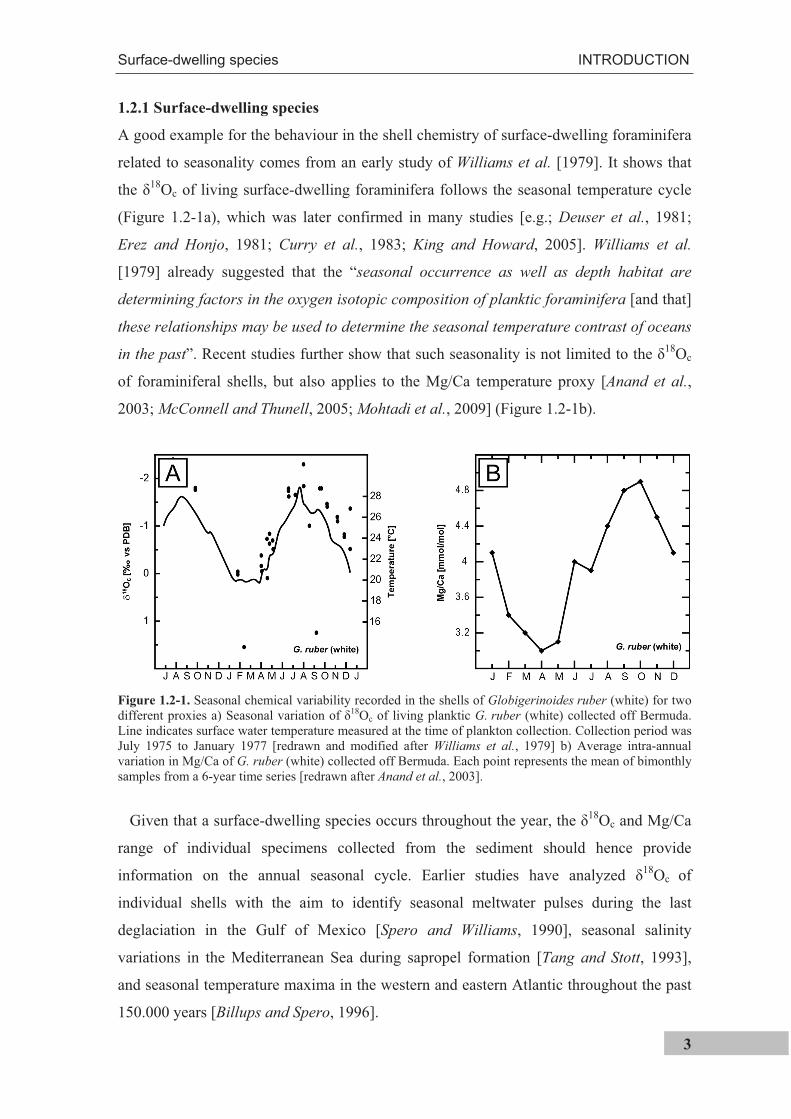
A good example for the behaviour in the shell chemistry of surface-dwelling foraminifera
related to seasonality comes from an early study of Williams et al. [1979]. It shows that
the 18Oc of living surface-dwelling foraminifera follows the seasonal temperature cycle
(Figure 1.2-1a), which was later confirmed in many studies [e.g.; Deuser et al., 1981;
Erez and Honjo, 1981; Curry et al., 1983; King and Howard, 2005]. Williams et al.
[1979] already suggested that the “seasonal occurrence as well as depth habitat are
determining factors in the oxygen isotopic composition of planktic foraminifera [and that]
these relationships may be used to determine the seasonal temperature contrast of oceans
in the past”. Recent studies further show that such seasonality is not limited to the 18Oc
of foraminiferal shells, but also applies to the Mg/Ca temperature proxy [Anand et al.,
2003; McConnell and Thunell, 2005; Mohtadi et al., 2009] (Figure 1.2-1b).
Figure 1.2-1. Seasonal chemical variability recorded in the shells of Globigerinoides ruber (white) for two different proxies a) Seasonal variation of 18Oc of living planktic G. ruber (white) collected off Bermuda. Line indicates surface water temperature measured at the time of plankton collection. Collection period was July 1975 to January 1977 [redrawn and modified after Williams et al., 1979] b) Average intra-annual variation in Mg/Ca of G. ruber (white) collected off Bermuda. Each point represents the mean of bimonthly samples from a 6-year time series [redrawn after Anand et al., 2003].
Given that a surface-dwelling species occurs throughout the year, the 18Oc and Mg/Ca
range of individual specimens collected from the sediment should hence provide
information on the annual seasonal cycle. Earlier studies have analyzed 18Oc of
individual shells with the aim to identify seasonal meltwater pulses during the last
deglaciation in the Gulf of Mexico [Spero and Williams, 1990], seasonal salinity
variations in the Mediterranean Sea during sapropel formation [Tang and Stott, 1993],
and seasonal temperature maxima in the western and eastern Atlantic throughout the past
150.000 years [Billups and Spero, 1996].
INTRODUCTION Surface-dwelling species
4
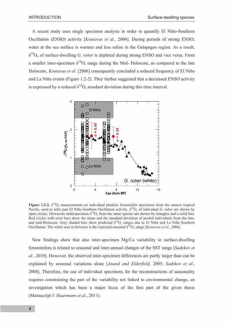
A recent study uses single specimen analysis in order to quantify El Niño-Southern
Oscillation (ENSO) activity [Koutavas et al., 2006]. During periods of strong ENSO,
water at the sea surface is warmer and less saline in the Galapagos region. As a result, 18Oc of surface-dwelling G. ruber is depleted during strong ENSO and vice versa. From
a smaller inter-specimen 18Oc range during the Mid- Holocene, as compared to the late
Holocene, Koutavas et al. [2006] consequently concluded a reduced frequency of El Niño
and La Niña events (Figure 1.2-2). They further suggested that a decreased ENSO activity
is expressed by a reduced 18Oc standard deviation during this time interval.
Figure 1.2-2. 18Oc measurements on individual planktic foraminifer specimens from the eastern tropical
Pacific, used to infer past El Niño-Southern Oscillation activity. 18Oc of individual G. ruber are shown by open circles. Downcore multispecimen 18Oc from the same species are shown by triangles and a solid line. Red circles with error bars show the mean and the standard deviation of pooled individuals from the late- and mid-Holocene. Grey shaded bars show predicted 18Oc ranges due to El Niño and La Niña Southern Oscillation. The white area in between is the expected seasonal 18Oc range [Koutavas et al., 2006].
New findings show that also inter-specimen Mg/Ca variability in surface-dwelling
foraminifera is related to seasonal and inter-annual changes of the SST range [Sadekov et
al., 2010]. However, the observed inter-specimen differences are partly larger than can be
explained by seasonal variations alone [Anand and Elderfield, 2005; Sadekov et al.,
2008]. Therefore, the use of individual specimens for the reconstructions of seasonality
requires constraining the part of the variability not linked to environmental change, an
investigation which has been a major focus of the first part of the given thesis
(Manuscript I: Haarmann et al., 2011).
Surface-dwelling species INTRODUCTION
5
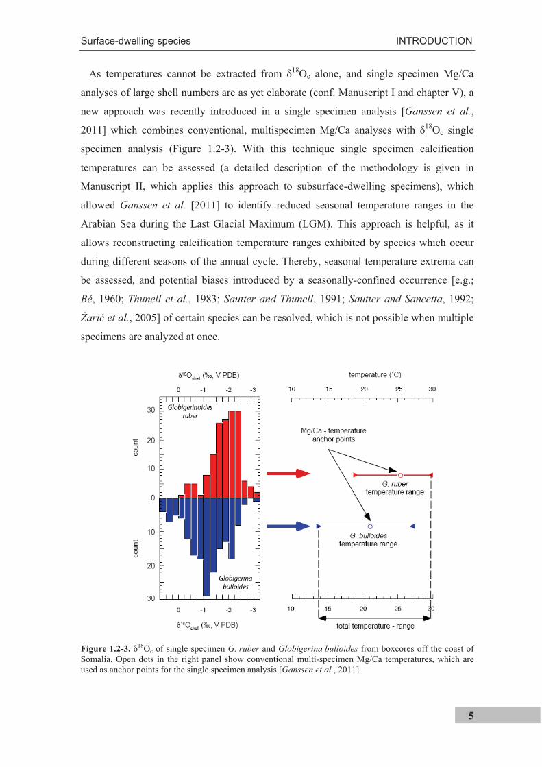
As temperatures cannot be extracted from 18Oc alone, and single specimen Mg/Ca
analyses of large shell numbers are as yet elaborate (conf. Manuscript I and chapter V), a
new approach was recently introduced in a single specimen analysis [Ganssen et al.,
2011] which combines conventional, multispecimen Mg/Ca analyses with 18Oc single
specimen analysis (Figure 1.2-3). With this technique single specimen calcification
temperatures can be assessed (a detailed description of the methodology is given in
Manuscript II, which applies this approach to subsurface-dwelling specimens), which
allowed Ganssen et al. [2011] to identify reduced seasonal temperature ranges in the
Arabian Sea during the Last Glacial Maximum (LGM). This approach is helpful, as it
allows reconstructing calcification temperature ranges exhibited by species which occur
during different seasons of the annual cycle. Thereby, seasonal temperature extrema can
be assessed, and potential biases introduced by a seasonally-confined occurrence [e.g.;
Bé, 1960; Thunell et al., 1983; Sautter and Thunell, 1991; Sautter and Sancetta, 1992;
Žari et al., 2005] of certain species can be resolved, which is not possible when multiple
specimens are analyzed at once.
Figure 1.2-3.18Oc of single specimen G. ruber and Globigerina bulloides from boxcores off the coast of
Somalia. Open dots in the right panel show conventional multi-specimen Mg/Ca temperatures, which are used as anchor points for the single specimen analysis [Ganssen et al., 2011].
INTRODUCTION Surface-dwelling species
6
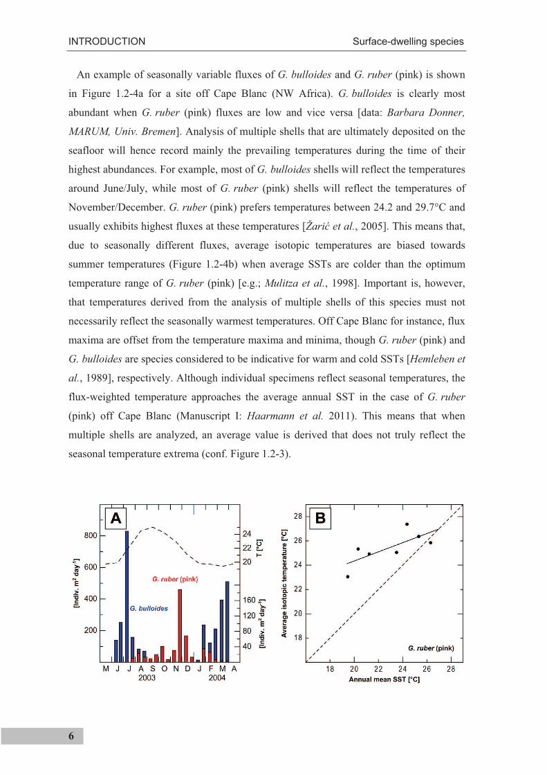
An example of seasonally variable fluxes of G. bulloides and G. ruber (pink) is shown
in Figure 1.2-4a for a site off Cape Blanc (NW Africa). G. bulloides is clearly most
abundant when G. ruber (pink) fluxes are low and vice versa [data: Barbara Donner,
MARUM, Univ. Bremen]. Analysis of multiple shells that are ultimately deposited on the
seafloor will hence record mainly the prevailing temperatures during the time of their
highest abundances. For example, most of G. bulloides shells will reflect the temperatures
around June/July, while most of G. ruber (pink) shells will reflect the temperatures of
November/December. G. ruber (pink) prefers temperatures between 24.2 and 29.7°C and
usually exhibits highest fluxes at these temperatures [Žari et al., 2005]. This means that,
due to seasonally different fluxes, average isotopic temperatures are biased towards
summer temperatures (Figure 1.2-4b) when average SSTs are colder than the optimum
temperature range of G. ruber (pink) [e.g.; Mulitza et al., 1998]. Important is, however,
that temperatures derived from the analysis of multiple shells of this species must not
necessarily reflect the seasonally warmest temperatures. Off Cape Blanc for instance, flux
maxima are offset from the temperature maxima and minima, though G. ruber (pink) and
G. bulloides are species considered to be indicative for warm and cold SSTs [Hemleben et
al., 1989], respectively. Although individual specimens reflect seasonal temperatures, the
flux-weighted temperature approaches the average annual SST in the case of G. ruber
(pink) off Cape Blanc (Manuscript I: Haarmann et al. 2011). This means that when
multiple shells are analyzed, an average value is derived that does not truly reflect the
seasonal temperature extrema (conf. Figure 1.2-3).
Subsurface-dwelling species INTRODUCTION
7
Figure 1.2-4 (previous page). Seasonal variability in the shell flux of G. ruber (pink) and G. bulloides andits effect on the geochemical signal extracted from the sedimentary record. a) G. bulloides and G. ruber fluxes to sediment trap CBi3-o off Cape Blanc at 20°45’N, 18°41’W [data: Barbara Donner] and monthly average SST [Locarnini et al., 2006] b) Average G. ruber (pink) isotopic temperatures (dots) from classes of samples throughout different latitudes of the Atlantic Ocean versus average annual temperatures within these classes. The solid line shows the regression through the isotopic temperatures [redrawn from Mulitza et al., 1998].
Using single specimen analyses, also specimens are included in the analysis which lived
during the season of warmest/coldest temperatures, so that temperature extrema can be
assessed, both in specimens collected from the water column by means of a sediment trap
(Manuscript I: Haarmann et al. 2011) as well as in specimens from the sedimentary
record [Ganssen et al., 2011].
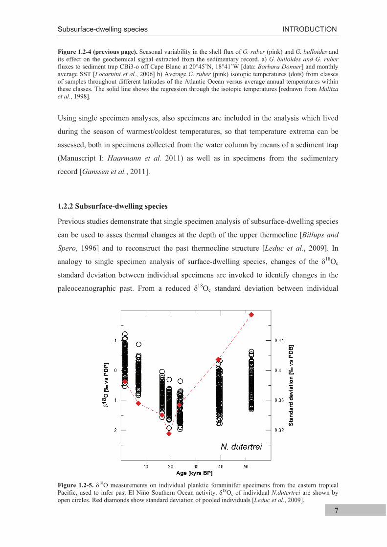
1.2.2 Subsurface-dwelling species
Previous studies demonstrate that single specimen analysis of subsurface-dwelling species
can be used to asses thermal changes at the depth of the upper thermocline [Billups and
Spero, 1996] and to reconstruct the past thermocline structure [Leduc et al., 2009]. In
analogy to single specimen analysis of surface-dwelling species, changes of the 18Oc
standard deviation between individual specimens are invoked to identify changes in the
paleoceanographic past. From a reduced 18Oc standard deviation between individual
Figure 1.2-5. 18O measurements on individual planktic foraminifer specimens from the eastern tropical
Pacific, used to infer past El Niño Southern Ocean activity. 18Oc of individual N.dutertrei are shown by open circles. Red diamonds show standard deviation of pooled individuals [Leduc et al., 2009].
INTRODUCTION Subsurface-dwelling species
8
shells of Neogloboquadrina dutertrei, Leduc et al. [2009] concluded reduced thermocline
variability and ENSO activity during the LGM as compared to the preceding glacial
(Figure 1.2-5). The interpretation of single subsurface-dwelling species is less
straightforward than for surface dwelling species, since the former migrate vertically
through the water column during their life cycle [Lon ari et al., 2006; Wilke et al.,
2006]. Therefore, despite little temperature changes throughout the year at subsurface
depths, large 18Oc and Mg/Ca differences are documented between individual specimens
[e.g.; Billups and Spero, 1996; Leduc et al., 2009; Haarmann et al., 2011]. In this thesis,
single specimens of the species Globorotalia inflata were investigated (Manuscript II).
Typical studies analyze multiple shells in order to derive an average calcification depth
considered representative of the whole population. These however vary between 100 and
600 m for G. inflata [Erez and Honjo, 1981; Elderfield and Ganssen, 2000; Ganssen and
Kroon, 2000; Anand et al. 2003; Chiessi et al., 2007; Groeneveld and Chiessi, 2011],
resulting from different depth habitats and/or the addition of secondary crust calcite
[Groeneveld and Chiessi, 2011]. As subsurface-dwelling species - in comparison to
surface-dwelling species - are valuable for the reconstruction of past ocean stratification
[e.g.; Mulitza et al., 1997; Rashid and Boyle, 2007], it is important to precisely constrain
their habitat (Manuscript I: Haarmann et al., 2011). In order to identify changes of the 18Oc standard deviation in the past, these are commonly compared to core top samples
[Leduc et al., 2009]. When calcification temperatures are assessed from individual fossil
shells, it is ideal to compare these to temperatures derived from specimens collected from
the water column, as is demonstrated in Manuscript II.
Assessing temperature extrema INTRODUCTION
9
1.3 Assessing temperature extrema
As has been cited above, Ganssen et al. [2011] have recently combined 18Oc
measurements of individual surface-dwelling specimens with multispecimen Mg/Ca
measurements in order to reconstruct surface temperature extrema for the
paleoceanographic past. In the present thesis, this approach was used to assess
calcification temperatures of subsurface-dwelling G. inflata for the past 22,000 years
(Manuscript II). Using this technique, single specimen temperatures are calculated as
follows.
(1) Multiple specimens (~30) collected from a sedimentary sample are analyzed
for their Mg/Ca ratios, using standard cleaning techniques [Barker et al.,
2003] and calcification temperatures are calculated [e.g.; Elderfield and
Ganssen, 2000; Anand et al., 2003].
(2) From the same sedimentary sample, individual specimens are collected and
analyzed for their 18Oc.
(3) The mean value of the individual 18Oc measurements is calculated. This
value is considered to reflect the mean of the whole fossil population. This is
also considered true for the value derived previously from the multiple-shell
Mg/Ca analysis.
(4) Consequently, the calculated Mg/Ca temperature is used to assign a
calcification temperature to the average 18Oc.
(5) Temperature extrema around this mean are then calculated using 18Oc:temperature relationships [e.g.; Bemis et al., 1998].
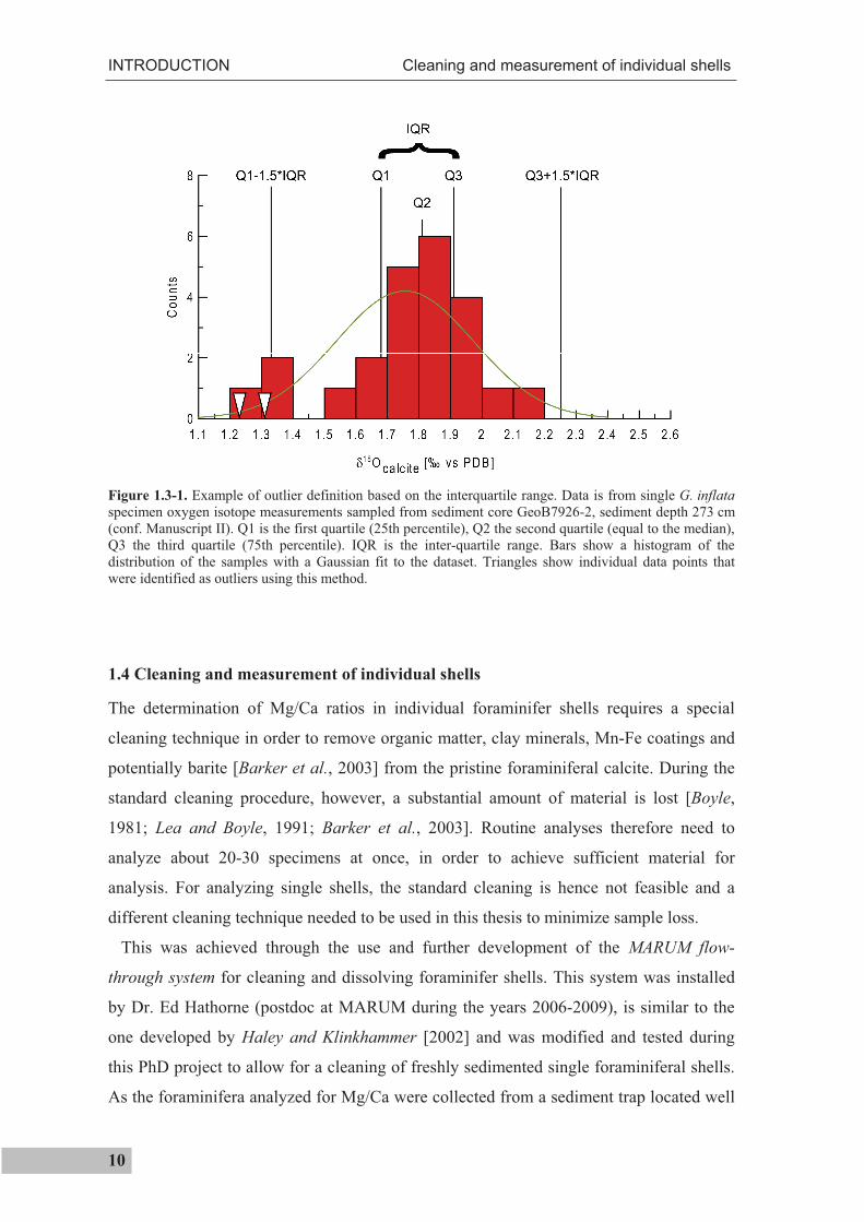
For the interpretation of temperature extrema as well as for the assumption that the
average 18Oc value truly represents the population mean, it is important that no bias is
introduced by potential outliers. The approach of Ganssen et al. [2011] uses the inter-
quartile range in order to identify outliers (Figure 1.3-1). An outlier is then defined as
being outside of the range (equation 1.3-1)
[Q1-1.5*(Q3-Q1), Q3+1.5*(Q3-Q1)] (1.3-1)
with Q3 and Q1 being the third and first quartile.
INTRODUCTION Cleaning and measurement of individual shells
10
Figure 1.3-1. Example of outlier definition based on the interquartile range. Data is from single G. inflataspecimen oxygen isotope measurements sampled from sediment core GeoB7926-2, sediment depth 273 cm (conf. Manuscript II). Q1 is the first quartile (25th percentile), Q2 the second quartile (equal to the median), Q3 the third quartile (75th percentile). IQR is the inter-quartile range. Bars show a histogram of the distribution of the samples with a Gaussian fit to the dataset. Triangles show individual data points that were identified as outliers using this method.
1.4 Cleaning and measurement of individual shells
The determination of Mg/Ca ratios in individual foraminifer shells requires a special
cleaning technique in order to remove organic matter, clay minerals, Mn-Fe coatings and
potentially barite [Barker et al., 2003] from the pristine foraminiferal calcite. During the
standard cleaning procedure, however, a substantial amount of material is lost [Boyle,
1981; Lea and Boyle, 1991; Barker et al., 2003]. Routine analyses therefore need to
analyze about 20-30 specimens at once, in order to achieve sufficient material for
analysis. For analyzing single shells, the standard cleaning is hence not feasible and a
different cleaning technique needed to be used in this thesis to minimize sample loss.
This was achieved through the use and further development of the MARUM flow-
through system for cleaning and dissolving foraminifer shells. This system was installed
by Dr. Ed Hathorne (postdoc at MARUM during the years 2006-2009), is similar to the
one developed by Haley and Klinkhammer [2002] and was modified and tested during
this PhD project to allow for a cleaning of freshly sedimented single foraminiferal shells.
As the foraminifera analyzed for Mg/Ca were collected from a sediment trap located well
Cleaning and measurement of individual shells INTRODUCTION
11
above the seafloor, only oxidative cleaning was performed, since only organic matter can
contaminate Mg/Ca measurements in the water column.
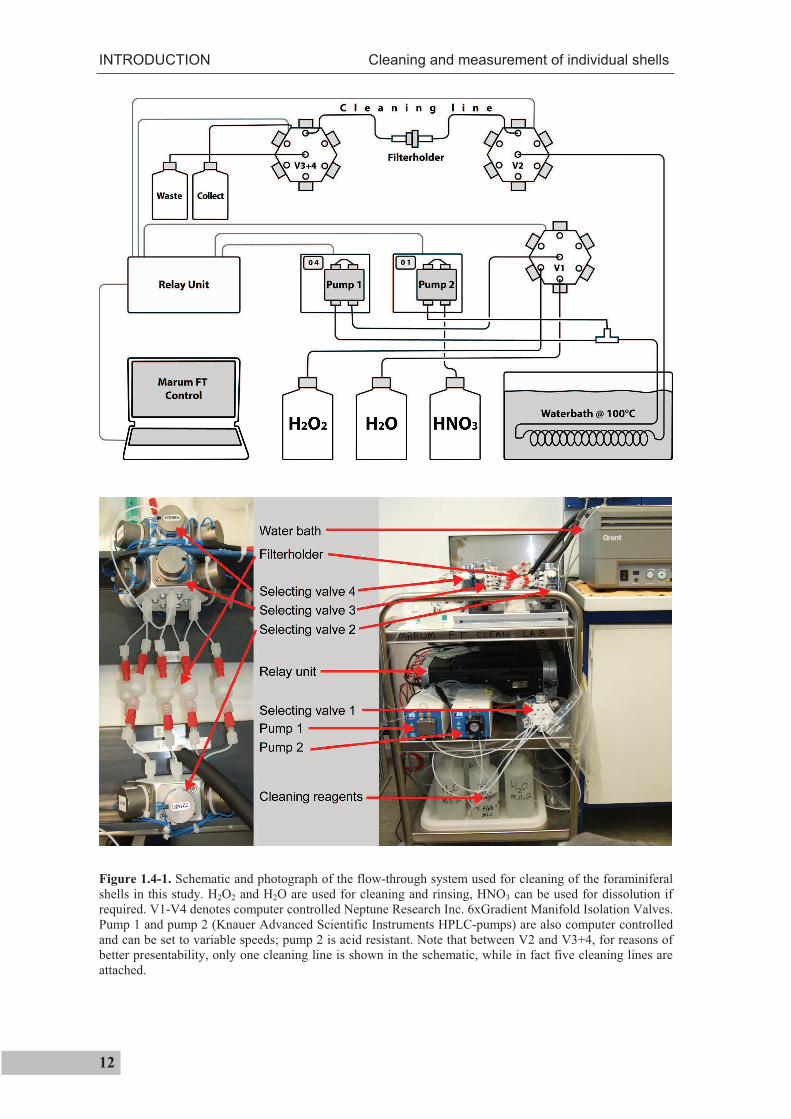
Figure 1.4-1 shows a schematic and photograph of the flow-through. In the system,
foraminiferal samples are placed in between two PTFE filters (Whatman International
Ltd.), kept in a filter holder that is arranged in the middle of a cleaning line (for reasons of
presentability, only one cleaning line is shown; in fact five cleaning lines are used). The
computer is then programmed to run a predefined cleaning procedure, so that the samples
in the filter holders are consecutively exposed to a constant flow of cleaning and rinsing
reagents. First, valve 1 (V1; Neptune Research Inc. 6xGradient Manifold Isolation
Valves) is used to select the needed reagent. The reagent is then pumped at a defined
speed using pump 1 (Knauer Advanced Scientific Instruments HPLC-pump K-120) and
passes a water bath (100°C), where it is heated up to ~60°C. Further downstream, V2 is
used to select one of the five cleaning lines. After passing the filter on which the sample
is located, V3 and V4 are used to direct the reagent towards waste. After a predefined
time, V1 is programmed to disconnect the first reagent (e.g.; H2O2) from the cleaning line
and connect the next reagent (e.g.; H2O for rinsing) to it. These steps are repeated for
every sample. The reagents used consecutively in this thesis were: Suprapure H2O2 (30%)
diluted to 1% in 0.1 M analytical grade NaOH (heated to ~60°C) for >20 min (pump
speed: 2 ml/min) followed by suprapure water (>18 M cm) for 46 min (pump speed:
6 min at 4 ml min-1, then 40 min at 1 ml min-1). To avoid dissolution during rinsing, the
pH of the deionised water was kept above 7 by adding a few drops of suprapure NH3
solution. After cleaning the single specimens were taken off the filter and examined under
a binocular microscope to determine if they remained intact during cleaning. They were
then transferred to clean vials, dissolved in 500 µL thermally distilled 0.075 M HNO3 and
centrifuged for 10 min at 6000 rpm prior to trace metal analysis. This cleaning procedure
produced good results for the cleaning of freshly deposited foraminifer shells. Quick and
efficient cleaning procedure for sedimentary shells is also desirable for sedimentary
shells. This requires a different approach that also includes dissolution of the
foraminiferal shells in the flow-through system. Therefore, a second, acid-resistant pump
(pump 2) is attached to the system. Through this pump, dissolution reagent (HNO3) can
be mixed to the stream of solution. After passing the sample, V3 and V4 are then
switched to a configuration that directs the solution to collecting vials. A summary of the
efforts and results for developing a cleaning procedure for sedimentary shells is given in
chapter V.
INTRODUCTION Cleaning and measurement of individual shells
12
Figure 1.4-1. Schematic and photograph of the flow-through system used for cleaning of the foraminiferal shells in this study. H2O2 and H2O are used for cleaning and rinsing, HNO3 can be used for dissolution if required. V1-V4 denotes computer controlled Neptune Research Inc. 6xGradient Manifold Isolation Valves. Pump 1 and pump 2 (Knauer Advanced Scientific Instruments HPLC-pumps) are also computer controlled and can be set to variable speeds; pump 2 is acid resistant. Note that between V2 and V3+4, for reasons of better presentability, only one cleaning line is shown in the schematic, while in fact five cleaning lines are attached.
Cleaning and measurement of individual shells INTRODUCTION
13
As the thin shells of G. ruber (pink) and G. ruber (white) analyzed in this thesis
produce solutions with low Ca concentrations, determination of Mg/Ca ratios was
achieved using inductively coupled plasma mass spectrometry (ICP-MS), following the
method of Rosenthal et al. [1999]. Sample Ca concentrations were first measured on a
Perkin-Elmer Optima 3300R inductively coupled plasma-optical emission spectrometer
(ICP-OES) and then diluted to have Ca concentrations of 2 and 5 ppm. Standard solutions
having the same Ca concentrations were prepared gravimetrically from single element
solutions to have a Mg/Ca ratio of 4.90 mmol/mol (as expected for G. ruber (pink) and
G. ruber (white)). Mg and Ca intensities of the standards and the samples were measured
on a Thermo-Finnigan Element 2 sector field ICP-MS and corrected for intensities
measured in blank solutions. Mg/Ca ratios were then assessed directly from intensity
ratios. In contrast to determination of Mg/Ca ratios from concentrations, this approach has
the advantage that different sample dilutions have no effect on the accuracy of the
measurement [Rosenthal et al., 1999]. The sample Mg/Ca ratio is calculated as
(Mg/Ca)sample = C*(Mg/Ca)measured (1.4-1)
where C is a correction factor that accounts for deviations of the measured ratio from the
true ratio (here 4.90 mmol/mol).
C = (Mg/Ca)standard/(Mg/Ca)measured (1.4-2)

14
THESIS OUTLINE
15
II. THESIS OUTLINE
The goal of this thesis is to advance recent developments for the reconstruction of past ocean
temperature seasonality and thermal water column stratification, using single foraminiferal
shell Magnesium to Calcium ratios and oxygen isotope ratios. The results of the thesis are
presented in three separate manuscripts, as summarized below.
Manuscript 1: Mg/Ca ratios of single planktonic foraminifer shells and the potential to
reconstruct the thermal seasonality of the water column
Tim Haarmann, Ed C. Hathorne, Mahyar Mohtadi, Jeroen Groeneveld, Martin Kölling,
Torsten Bickert
Paleoceanography, 26 (doi: 10.1029/2010PA002091)
This article addresses inter-specimen Mg/Ca variability in two surface-
(Globigerinoides ruber (white) and Globigerinoides ruber (pink)) and one intermediate-
depth dwelling (Globorotalia inflata) foraminiferal species collected from a sediment trap
off NW Africa. For G. ruber (pink) we could confirm recent hypotheses [Sadekov et al.,
2008; Wit et al., 2010] that single shell Mg/Ca ratios are related to seasonal sea surface
temperature (SST). For G. inflata we show that this species exhibits little Mg/Ca seasonality
and that single shells reflect temperatures between the sea surface and ~400 m water depth.
The sediment trap time series suggests that for specimens collected from the sedimentary
record detectable changes in the past temperature range under which these species calcified
correspond to changes of the Mg/Ca ratios 0.80 mmol/mol (G. ruber (pink)) and
0.34 mmol/mol (G. inflata). This study was enabled by the further development of the
Marum flow-through system (chapter 1.4) for cleaning and dissolving foraminiferal shells.
THESIS OUTLINE
16
Manuscript 2: Subsurface thermal stratification off NW Africa during the past 24,000
years – inferences from single planktic foraminifer shells
Tim Haarmann, Frank Peeters, Gerald Ganssen, Ute Merkel, Torsten Bickert
For submission to Paleoceanography
This study is a continuation of the preceding study and tests the suggested potential of single
specimens of G. inflata for reconstructing the past thermal ocean stratification at the study
site. Conventional multi-specimen Mg/Ca analysis was combined with single specimen 18Oc analysis (chapter 1.3) in order to assess past subsurface calcification temperatures of
single specimens of this species off NW Africa for the past 22,000 years. The selection of a
sediment core at the same site as the sediment trap allowed for excellent comparability to the
present day observations and showed that near present (570 years before present) single
sedimentary G. inflata shells reflect present day calcification temperature ranges of this
species well. However, during the last deglaciation, the calcification temperature range of
G. inflata was significantly reduced. Statistical analysis and comparison to past subsurface
water column stratification derived from the Community Climate System Model Version 3
(CCSM3) suggests that G. inflata inhabited a substantially reduced habitat range during the
deglaciation, as a result of stronger water column stratification. Single specimen 18Oc
analyses were carried out in collaboration with the project partners at the Vrije Universiteit
Amsterdam.
Manuscript 3: Upwelling strength off Cape Blanc (NW Africa) during the past
24,000 BP – Effects on the surface and subsurface Mg/Ca temperature records
Tim Haarmann, Mahyar Mohtadi, Jeroen Groeneveld, Torsten Bickert
In preparation for Biogeosciences
In this manuscript, the previously investigated surface- and subsurface dwelling species are
used in a conventional, multispecimen Mg/Ca temperature analysis at the study site for the
past 24,000 years. At this site, previous studies suggest unexpectedly warm SSTs during
generally cold climatic states as a result of decreased upwelling of cold subsurface waters
[Romero et al., 2008]. The present thesis contradicts this suggestion and reconstructed strong
upwelling from high relative abundances of G. bulloides between 24,000 and 16,000 years
THESIS OUTLINE
17
before present. Mg/Ca temperatures reconstructed from the surface-dwelling species
G. ruber (pink) and G. bulloides are generally highly variable, in contrast to those of
subsurface-dwelling G. inflata. Concluded by modern analogy, we explain the high SST
variability at the study site during strong upwelling with substantial temperature differences
at the sea surface, likely through the advection of warm tropical surface waters towards the
study area.
Future studies are needed to test this hypothesis and could be done by analyzing single shells
of G. ruber (pink) and G. bulloides in order to work out temperature extrema at the study
site. This could be achieved through a combined approach of multi-specimen Mg/Ca and
single specimen 18Oc analysis, as used in Manuscript II. More directly, Mg/Ca ratios would
be analyzed from single sedimentary shells. This requires a further development of the
cleaning technique for single foraminiferal shells. An outlook for such future developments
is given in chapter V.

18
MATERIAL AND STUDY SITE
19
III. MATERIAL AND STUDY SITE
3.1 Samples
This thesis aims to compare recent single foraminiferal specimens from the water column
to their fossil, sedimentary counterparts. For this reason, recent samples were collected
from a sediment trap and compared to fossil samples collected from a sediment core as
close as possible to the sediment trap location. The sediment trap (CBi3-o) was moored
~170 km off Cape Blanc, NW Africa (20°45.6’N, 18°41.9’W) at 1277 meters below sea
level, 1416 meters above sea floor. The gravity core GeoB7926-2 was recovered at
20°12.8’N, 18°27.1’W at 2500 m water depth. Coretop samples were obtained from the
top centimeter of multicorer GeoB7408-2 at 20°17.4’N, 18°15.0’W from a water depth of
1935 m. Details on the recovery and sampling procedure are provided in Manuscripts I
(sediment trap and coretop samples) and II (sediment core). A revised age model for the
previously dated sediment core GeoB7926-2 [Romero et al., 2008] is presented in
Manuscript II. The sediment trap, sediment core and top centimeter of the multicorer were
sampled for G. ruber (pink) and G. inflata. In addition, the sediment trap was sampled for
G. ruber (white) and the sediment core for G. bulloides.
3.2 Study site
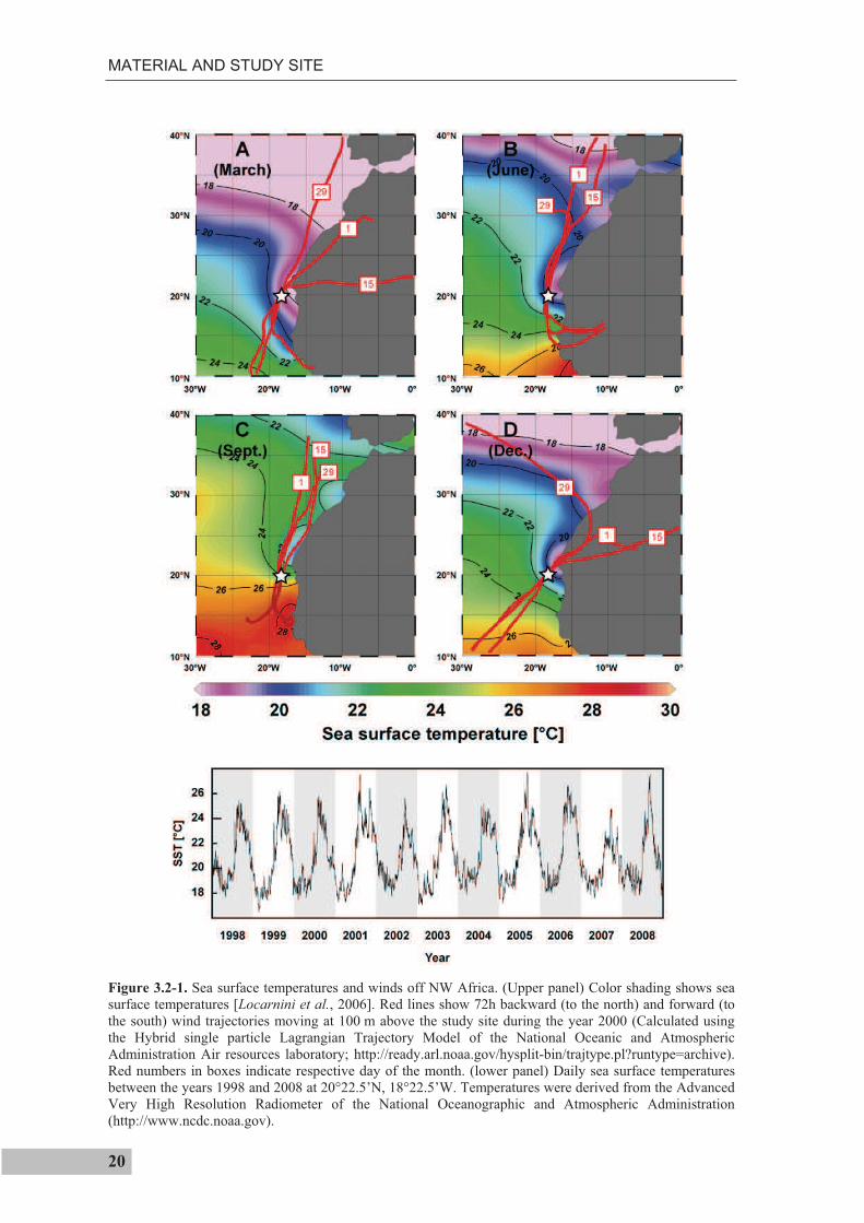
The study site off Cape Blanc is dominated by the seasonal migration of the Inter Tropical
Convergence Zone (ITCZ) between ~5° and 20°N and the seasonal migration of the
northeast trade winds (Figure 3.2-1), accompanied by a strong seasonal SST contrast and
a pronounced seasonal thermocline. The amplitude of the annual temperature cycle at the
surface is 5.3°C, and at the depth of the seasonal thermocline (~75 m) about 0.8°C,
whereas at 300 m the seasonal temperature range is only 0.3°C [Locarnini et al., 2006].
The surface temperature range can, however, be significantly larger, if daily temperatures
are considered (Figure 3.2-1). The trade winds modulate the southward flowing Canary
Current and the northward flowing Mauritania current (Figure 3.2-2a). During winter, the
Canary Current reaches furthest south. In summer, when the southern boundary of the
trade winds has its northernmost position, the coastal northward flowing current advects
warm waters up to the latitude of Cape Blanc [Mittelstaedt, 1983].
MATERIAL AND STUDY SITE
20
Figure 3.2-1. Sea surface temperatures and winds off NW Africa. (Upper panel) Color shading shows sea surface temperatures [Locarnini et al., 2006]. Red lines show 72h backward (to the north) and forward (to the south) wind trajectories moving at 100 m above the study site during the year 2000 (Calculated using the Hybrid single particle Lagrangian Trajectory Model of the National Oceanic and Atmospheric Administration Air resources laboratory; http://ready.arl.noaa.gov/hysplit-bin/trajtype.pl?runtype=archive). Red numbers in boxes indicate respective day of the month. (lower panel) Daily sea surface temperatures between the years 1998 and 2008 at 20°22.5’N, 18°22.5’W. Temperatures were derived from the Advanced Very High Resolution Radiometer of the National Oceanographic and Atmospheric Administration (http://www.ncdc.noaa.gov).
MATERIAL AND STUDY SITE
21
MATERIAL AND STUDY SITE
22
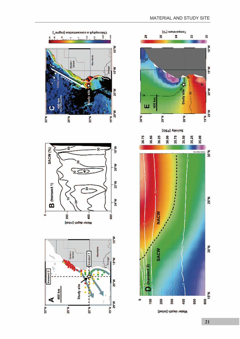
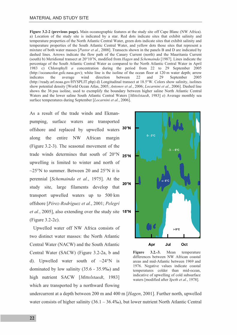
Figure 3.2-2 (previous page). Main oceanographic features at the study site off Cape Blanc (NW Africa). a) Location of the study site is indicated by a star. Red dots indicate sites that exhibit salinity and temperature properties of the North Atlantic Central Water, green dots indicate sites that exhibit salinity and temperature properties of the South Atlantic Central Water, and yellow dots those sites that represent a mixture of both water masses [Pastor et al., 2008]. Transects shown in the panels B and D are indicated by dashed lines. Arrows indicate the flow path of the Canary Current (north) and the Mauritania Current (south) b) Meridional transect at 20°10’N, modified from Hagen and Schemainda [1987]. Lines indicate the percentage of the South Atlantic Central Water as compared to the North Atlantic Central Water in April 1983 c) Chlorophyll a concentration during the period from 22 to 29 September 2005 (http://oceancolor.gsfc.nasa.gov); white line is the isoline of the ocean floor at 120 m water depth; arrow indicates the average wind direction between 22 and 29 September 2005 (http://ready.arl.noaa.gov/HYSPLIT.php) d) Longitudinal transect at 18.5°W. Colors show salinity, isolines show potential density [World Ocean Atlas, 2005; Antonov et al., 2006; Locarnini et al., 2006]. Dashed line shows the 36 psu isoline, used to exemplify the boundary between higher saline North Atlantic Central Waters and the lower saline South Atlantic Central Waters [Mittelstaedt, 1983] e) Average monthly sea surface temperatures during September [Locarnini et al., 2006].
As a result of the trade winds and Ekman-
pumping, surface waters are transported
offshore and replaced by upwelled waters
along the entire NW African margin
(Figure 3.2-3). The seasonal movement of the
trade winds determines that south of 20°N
upwelling is limited to winter and north of
~25°N to summer. Between 20 and 25°N it is
perennial [Schemainda et al., 1975]. At the
study site, large filaments develop that
transport upwelled waters up to 500 km
offshore [Pérez-Rodríguez et al., 2001; Pelegrí
et al., 2005], also extending over the study site
(Figure 3.2-2c).
Upwelled water off NW Africa consists of
two distinct water masses: the North Atlantic
Central Water (NACW) and the South Atlantic
Central Water (SACW) (Figure 3.2-2a, b and
d). Upwelled water south of ~24°N is
dominated by low salinity (35.6 - 35.9‰) and
high nutrient SACW [Mittelstaedt, 1983]
which are transported by a northward flowing
undercurrent at a depth between 200 m and 400 m [Hagen, 2001]. Further north, upwelled
water consists of higher salinity (36.1 – 36.4‰), but lower nutrient North Atlantic Central
Figure 3.2.-3. Mean temperature differences between NW African coastal areas and mid-Atlantic between 1969 and 1976. Negative values indicate coastal temperatures colder than mid-ocean, indicative of upwelling of cold subsurface waters [modified after Speth et al., 1978].
MATERIAL AND STUDY SITE
23
Water (NACW) [Mittelstaedt, 1983]. At the study site, both water masses converge and
the upwelled water is a mix of NACW and SACW. Because NACW and SACW have the
same density (Figure 3.2-2d), mixing and interleaving is facilitated (Figure 3.2-2b).

24
Mg/Ca ratios of single planktonic foraminifer shells MANUSCRIPTS
25
IV. MANUSCRIPTS
4.1 Manuscript 1
Mg/Ca ratios of single planktonic foraminifer shells and the potential to reconstruct
the thermal seasonality of the water column
Tim Haarmann1, Ed C. Hathorne
2, Mahyar Mohtadi
1, Jeroen Groeneveld
1, 3, Martin
Kölling4, Torsten Bickert
1
1Marum – Center for Marine Environmental Sciences, Leobener Straße, 28359 Bremen, Germany 2IFM-GEOMAR, Leibniz Institute for Marine Sciences at the University of Kiel, Wischhofstraße
1-3, 24148 Kiel, Germany 3Alfred Wegener Institute, Am Handelshafen 12, 27570 Bremerhaven, Germany 4University of Bremen, Department of Geosciences, Klagenfurter Straße 2, 28334 Bremen,
Germany
Published in Paleoceanography, 26 (doi: 10.1029/2010PA002091) as editor’s highlight and
summarized as research spotlight in Eos, 92 (43), 25 October 2011
Mg/Ca ratios of surface- and subsurface dwelling foraminifera provide valuable
information about the past temperature of the water column. Planktonic foraminifera
calcify over a period of weeks to months. Therefore, the range of Mg/Ca temperatures
obtained from single specimens potentially records seasonal temperature changes. We
present solution derived Mg/Ca ratios for single specimens of the planktonic foraminifera
species Globigerinoides ruber (pink), Globigerinoides ruber (white), and Globorotalia inflata,
from a sediment trap off NW Africa (20°45.6’N, 18°41.9’W). Cleaning of single specimens
was achieved using a flow-through system in order to prevent sample loss. Mg/Ca ratios of
surface dwelling G. ruber (pink) show strong seasonality linked to sea surface temperature.
Mg/Ca ratios of G. ruber (white) do not show such seasonality. Subsurface dwelling
G. inflata flux is largest during the main upwelling season but Mg/Ca ratios reflect annual
temperatures at intermediate water depths.
The sediment trap time-series suggests that changes in the range of Mg/Ca ratios exhibited
by single specimens of G. ruber (pink) and G. inflata from the sedimentary record should
provide information on the past temperature range under which these species calcified.
Statistical analysis suggests detectable changes in the Mg/Ca range are 0.80 mmol/mol
(G. ruber (pink)) and 0.34 mmol/mol (G. inflata). For G. ruber (pink), such changes would
MANUSCRIPTS Mg/Ca ratios of single planktonic foraminifer shells
26
indicate changes in the seasonal sea surface temperature range >4°C or a shift in the main
calcification and reproductive period. For G. inflata, such changes would indicate >1.7°C
changes in the thermocline temperature or a change in the depth habitat.
4.1.1 Introduction
Planktonic foraminifer Mg/Ca ratios are
important for reconstructing changes in sea
surface temperature (SST) [e.g. Elderfield
and Ganssen, 2000; Dekens et al., 2008]
and water column temperatures [e.g.
Cléroux et al., 2007; 2008] related to
climatic change. Numerous studies have
shown that the Mg content of the shells of
foraminifera correlates positively with the
water temperature during calcification [e.g.
Nürnberg et al., 1996; Lea, 1999;
Elderfield and Ganssen, 2000; Anand et
al., 2003; Cléroux et al., 2007; Dekens et
al., 2008]. Mg/Ca-temperature calibrations
are based on laboratory experiments [e.g.
Nürnberg et al., 1996], core top
calibrations [e.g. Elderfield and Ganssen,
2000; Cléroux et al., 2007; Groeneveld and
Chiessi, 2011] or sediment trap studies
[Anand et al., 2003; McConnell and
Thunell, 2005]. As such the Mg/Ca ratio of
planktonic foraminifera shells is commonly
used as a proxy for reconstructing the
temperature at the depth in which the
utilized species preferentially calcify. The
calcification depth of planktonic
foraminifera differs for various species.
Therefore, a thorough understanding of
foraminifer ecology and species specific
calibration is needed in order to reconstruct
past ocean temperatures with confidence.
Globigerinoides ruber (pink) is a tropical
to subtropical species [Hemleben et al.,
1989] and lives predominantly in the upper
50 m of the water column [e.g. Bé, 1977]
preferentially calcifying in the upper 25 m
[e.g. Ravelo et al., 1990; Anand et al.,
2003; Tedesco et al., 2007; Steph et al.,
2009]. Ganssen and Kroon [2000] suggest
G. ruber (pink) is restricted to temperatures
above 20°C, while Žari et al. [2005]
report a wider tolerance range of 16.4 -
29.6°C. G. ruber (pink)
Globigerinoides ruber (white) is a
tropical to transitional, mixed layer
dwelling species [e.g. Bé, 1977; Ganssen
and Kroon, 2000; Mohtadi et al., 2009]
and has a slightly wider temperature
tolerance range than G. ruber (pink). It
possesses photosynthetic algal symbionts
and favors a life in the photic zone, where
it is found in significant numbers
[Fairbanks et al., 1982], migrating
between the upper photic zone and the
chlorophyll maximum [Wilke et al., 2009].
Globorotalia inflata is a transitional to
subpolar species [Hemleben et al., 1989],
and lives in waters with a temperature
Mg/Ca ratios of single planktonic foraminifer shells MANUSCRIPTS
27
range between 8 and 18°C [e.g. Bé and
Hamlin, 1967; Farmer et al., 2010]. It is
very abundant in the upwelling region off
NW Africa, where it constitutes 25% of the
recent sedimentary planktonic foraminifers
[Diester-Haass et al., 1973]. The apparent
calcification depth of G. inflata is
suggested to vary between 100 and 600 m
[Erez and Honjo, 1981; Elderfield and
Ganssen, 2000; Ganssen and Kroon, 2000;
Anand et al., 2003; Chiessi et al., 2007;
Groeneveld and Chiessi, 2011]. Like many
species, G. inflata adds crust calcite to its
primary calcite test at greater depth and
colder temperatures [e.g. Caron et al.,
1990]. This can bias geochemical signals to
a deeper apparent calcification depth
[Groeneveld and Chiessi, 2011; van Raden
et al., 2011], although the difference in
Mg/Ca between crust and primary calcite
cannot be explained entirely by depth
migration [Hathorne et al., 2009]. G.
inflata abundance has been found in the
subsurface seasonal thermocline and the
mixed layer, coincident with the maximum
chlorophyll a concentration [Ravelo et al.,
1990; Wilke et al., 2006]. As such,
G. inflata has been used to reconstruct
water temperatures around the seasonal
thermocline [Cléroux et al., 2007, 2008].
G. inflata has small symbiotic algae
[Gastrich, 1987], restricting it to the photic
zone during at least part of its life cycle.
Planktonic foraminifera calcify over a
period of a couple of weeks to months [e.g.
Bé and Spero, 1981; Hemleben et al.,
1989], with the reproductive cycle often
triggered by the synodic lunar cycle [e.g.
Spindler et al., 1979; Bijma and Hemleben,
1990]. Single specimens thus potentially
record short-term temperature variations.
However, in standard geochemical
analyses, this potential is not exploited, as
traditionally, multiple (about 10 to 30)
specimens are analysed at once. This is
necessary in order to obtain a
representative average temperature, and to
achieve sufficient material for a reliable
analysis since a substantial amount of
material can be lost during standard
cleaning procedures [Boyle, 1981; Lea and
Boyle, 1991; Barker et al., 2003]. Analyses
using standard cleaning techniques can
therefore only provide average
temperatures, which may additionally be
biased towards the main reproductive
period of the species.
The importance of single shell 18O
analyses of planktonic foraminifera for
paleoceanographic questions is becoming
increasingly recognized [Spero and
Williams, 1989] and such analyses have
been applied to quantify past El Niño-
Southern Oscillation (ENSO) and
thermocline variance [Koutavas at al.,
2006; Leduc et al., 2009]. Recently, laser
ablation inductively coupled plasma-mass
spectrometry (LA-ICP-MS) has been used
MANUSCRIPTS Mg/Ca ratios of single planktonic foraminifer shells
28
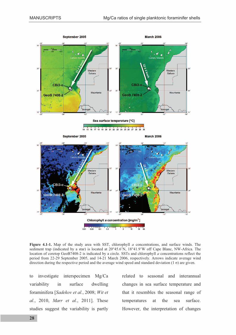
Figure 4.1-1. Map of the study area with SST, chlorophyll a concentrations, and surface winds. The sediment trap (indicated by a star) is located at 20°45.6’N, 18°41.9’W off Cape Blanc, NW-Africa. The location of coretop GeoB7408-2 is indicated by a circle. SSTs and chlorophyll a concentrations reflect the period from 22-29 September 2005, and 14-21 March 2006, respectively. Arrows indicate average wind direction during the respective period and the average wind speed and standard deviation (1 ) are given.
to investigate interspecimen Mg/Ca
variability in surface dwelling
foraminifera [Sadekov et al., 2008; Wit et
al., 2010, Marr et al., 2011]. These
studies suggest the variability is partly
related to seasonal and interannual
changes in sea surface temperature and
that it resembles the seasonal range of
temperatures at the sea surface.
However, the interpretation of changes
Mg/Ca ratios of single planktonic foraminifer shells MANUSCRIPTS
29
of the Mg/Ca variability for
paleoceanographic reconstructions
requires natural Mg/Ca variability, not
linked to environmental change, to be
well defined. Here we constrain this
natural Mg/Ca variability for G. ruber
(pink), G. ruber (white) and G. inflata
from a sediment trap time series.
In this study, we utilized a flow-
through system [Haley and
Klinkhammer, 2002], enabling Mg/Ca
measurements on single shells of
planktonic foraminifera from a sediment
trap off Cape Blanc, Mauritania, NW
Africa, (20°45.6’N, 18°41.9’W). We test
several Mg/Ca temperature equations for
their applicability to single specimens of
three planktonic foraminiferal species
(G. ruber (white), G. ruber (pink), G.
inflata) and investigate the potential of
single tests to assess short term
temperature variations. We further
evaluate and explain the variability in
Mg/Ca temperatures among single
specimens of these species, with a focus
on their potential applicability in
paleoceanographic studies.
4.1.2 Study area
The study area off Cape Blanc (NW-
Africa) is dominated by the seasonal
migration of the Inter Tropical
Convergence Zone (ITCZ), accompanied
by a strong seasonal SST contrast
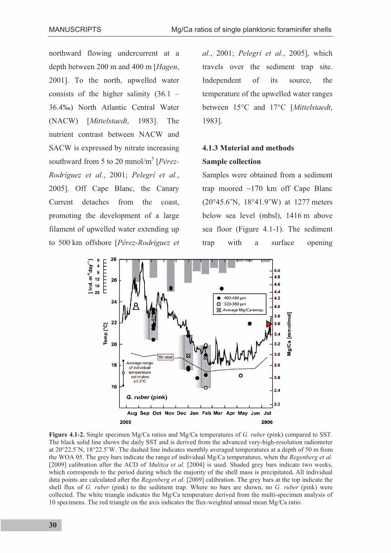
(Figure 4.1-1). The amplitude of the
annual SST cycle (Figure 4.1-2) derived
from the advanced very-high-resolution
radiometer at 20°22.5’N and 18°22.5’W
(http://www.ncdc.noaa.gov) was 9.6°C
during the deployment period with
highest temperatures in mid September
(27.7°C) and lowest temperatures in mid
March (18.1°C). This large annual
amplitude of SST is ideal for our study.
The main surface current in the study
area is the Canary Current, which flows
south along the NW African coast as the
eastern branch of the North Atlantic
Subtropical Gyre. The Canary Current is
modulated by south westward directed
trade winds (Figure 4.1-1) which blow
throughout the year between 20°N and
25°N [Schemainda et al., 1975] and
cause perennial upwelling off Cape
Blanc. Upwelling is strongest in late
spring and autumn [Ganssen and
Sarnthein, 1983; Pelegrí et al., 2005]. As
a result of the steady trade winds and
Ekman-pumping, surface waters are
transported offshore and replaced by
upwelled waters. The upwelled water off
NW Africa consists of two distinct water
masses: the North Atlantic Central Water
(NACW) and the South Atlantic Central
Water (SACW). Generally, to the south
of 24°N, upwelled water is dominated by
low salinity (35.6 - 35.9‰) SACW
[Mittelstaedt, 1983] transported by a
MANUSCRIPTS Mg/Ca ratios of single planktonic foraminifer shells
30
northward flowing undercurrent at a
depth between 200 m and 400 m [Hagen,
2001]. To the north, upwelled water
consists of the higher salinity (36.1 –
36.4‰) North Atlantic Central Water
(NACW) [Mittelstaedt, 1983]. The
nutrient contrast between NACW and
SACW is expressed by nitrate increasing
southward from 5 to 20 mmol/m3 [Pérez-
Rodríguez et al., 2001; Pelegrí et al.,
2005]. Off Cape Blanc, the Canary
Current detaches from the coast,
promoting the development of a large
filament of upwelled water extending up
to 500 km offshore [Pérez-Rodríguez et
al., 2001; Pelegrí et al., 2005], which
travels over the sediment trap site.
Independent of its source, the
temperature of the upwelled water ranges
between 15°C and 17°C [Mittelstaedt,
1983].
4.1.3 Material and methods
Sample collection
Samples were obtained from a sediment
trap moored ~170 km off Cape Blanc
(20°45.6’N, 18°41.9’W) at 1277 meters
below sea level (mbsl), 1416 m above
sea floor (Figure 4.1-1). The sediment
trap with a surface opening
Figure 4.1-2. Single specimen Mg/Ca ratios and Mg/Ca temperatures of G. ruber (pink) compared to SST. The black solid line shows the daily SST and is derived from the advanced very-high-resolution radiometer at 20°22.5’N, 18°22.5’W. The dashed line indicates monthly averaged temperatures at a depth of 50 m from the WOA 05. The grey bars indicate the range of individual Mg/Ca temperatures, when the Regenberg et al.[2009] calibration after the ACD of Mulitza et al. [2004] is used. Shaded grey bars indicate two weeks, which corresponds to the period during which the majority of the shell mass is precipitated. All individual data points are calculated after the Regenberg et al. [2009] calibration. The grey bars at the top indicate the shell flux of G. ruber (pink) to the sediment trap. Where no bars are shown, no G. ruber (pink) were collected. The white triangle indicates the Mg/Ca temperature derived from the multi-specimen analysis of 10 specimens. The red triangle on the axis indicates the flux-weighted annual mean Mg/Ca ratio.
Mg/Ca ratios of single planktonic foraminifer shells MANUSCRIPTS
31
of 0.5 m2 was equipped with 20 collecting
cups and poisoned with HgCl2. Samples
were collected in intervals of 21.5 days
between 25 July 2005 and 28 September
2006. Recovery and redeployment took
place during R/V Poseidon cruise 344
[Fischer et al., 2008]. Every cup was
divided into 5 aliquots using a rotating
splitter, of which one was used for this
study. When possible, additional aliquots
were used to obtain enough specimens for
analysis. The shallow depth of the
sediment trap precludes any dissolution of
the samples. Specimens of ~420 µm size
(as used in this study) sink at 1295 m day-1
[Takahashi and Bé, 1984] and thus reach
the sediment trap within about one day.
With an approximate eddy kinetic energy
of 40 cm2 s-2 at the study site [Hecht and
Hasumi, 2008] the horizontal averaging
scale for a sediment trap at 1000 m depth
ranges between 1 and 10 km [Siegel et al.,
1990].
The top centimeter of multicore GeoB
7408-2 at 20°17.4’N, 18°15.0’W from a
water depth of 1935 m, obtained during
R/V Poseidon cruise 272 [Meggers et al.,
2002] was used to study sedimentary
shells.
Individual specimens were picked and
their size and morphology noted under the
binocular microscope. Most G. inflata
(d’Orbigny) specimens had four chambers
in the last whorl and had moderately
thickened walls. All G. ruber specimens
were strictly from the G. ruber sensu
stricto morphotype [Wang, 2000].
Cleaning procedures
As the foraminifera originate from a
sediment trap that was located well above
the sea floor, only oxidative cleaning was
performed as organic matter can
contaminate Mg/Ca measurements [e.g.
Hastings et al., 1996; Barker et al., 2003].
We used a flow-through system [Haley and
Klinkhammer, 2002] run offline to clean
single specimens with minimal sample
loss. Sample loss is significant using
traditional cleaning techniques [Boyle,
1981; Barker et al., 2003] especially with
small sample sizes. In the flow-through
system, we placed single specimens
between two PTFE filters and subjected
them to a constant flow (2 ml min-1) of
suprapure H2O2 (30%) diluted to 1% in
0.1 M analytical grade NaOH (heated to
~60°C) for >20 min. The samples were
then rinsed for 46 min in a flow (6 min at
4 ml min-1, then 40 min at 1 ml min-1) of
pure water (>18 M cm). To avoid
dissolution during rinsing, the pH of the
deionised water was kept above 7 by
adding a few drops of suprapure NH3
solution. After cleaning individuals were
taken off the filter, examined under the
binocular microscope to determine if they
remained intact during cleaning, before
MANUSCRIPTS Mg/Ca ratios of single planktonic foraminifer shells
32
being transferred to clean vials and
dissolved in 500 µl thermally distilled (TD)
0.075M HNO3. Samples that broke during
cleaning are not considered. After
centrifugation for 10 min at 6000 rpm the
sample solution was transferred to clean
vials for measurement.
For multi-specimen analysis of sediment
samples, 10 G. inflata specimens were
picked from the 400-480 µm size fraction.
Cleaning was applied according to Barker
et al. [2003]. The solution was then
centrifuged (10 min at 6000 rpm) and
transferred into clean tubes and diluted for
measurement.
Data acquisition
Mg/Ca ratios were acquired using two
approaches: The thin shells of G. ruber
(pink and white) produced solutions with
low Ca concentrations requiring Mg/Ca
ratios to be determined with the more
sensitive inductively coupled plasma mass-
spectrometry (ICP-MS) technique. The Ca
concentrations of the sample solutions
were first measured on a Perkin-Elmer
Optima 3300R inductively coupled
plasma–optical emission spectrometer
(ICP-OES) equipped with an ultrasonic
nebulizer U-5000 AT (Cetac Technologies
Inc.) at the faculty of Geosciences,
University of Bremen. Samples for ICP-
MS analysis were then diluted to have Ca
concentrations of 2 or 5 ppm. Standard
solutions with the same Ca concentration
were prepared gravimetrically from single
element solutions to have Mg/Ca ratios of
4.90 mmol/mol (for measurements of G.
ruber (pink and white)) and
1.92 mmol/mol (for measurements of G.
inflata). Mg/Ca ratios were determined
using the method of Rosenthal et al. [1999]
from intensities measured on a Thermo-
Finnigan Element 2 sector field ICP-MS at
the University of Bremen. During this
study the measured Mg/Ca ratios of
carbonate reference materials ECRM 752-1
and JCt-1 diluted like the samples, were on
average 3.69 mmol/mol (n=19;
=0.03 mmol/mol), and 1.28 mmol/mol
(n=7; = 0.01 mmol/mol), respectively.
This is in good agreement with the reported
Mg/Ca ratios of 3.75 mmol/mol for the
ECRM 752-1 [Greaves et al., 2008] and
1.25 mmol/mol for the JCt-1 [Okai et al.,
2004]. All blanks analyzed were below the
average detection limits of 0.011 ppb Mg
and 1.49 ppb Ca.
The relatively thick shells of G. inflata
contained enough CaCO3 for the
determination of Mg/Ca ratios using ICP-
OES. Potential drift was monitored by
analysis of an in-house standard solution.
Values from different ICP-OES analytical
sessions were normalized using this
standard solution.
Mg/Ca ratios of G. ruber (pink), G. ruber
(white) and G. inflata were used to
Mg/Ca ratios of single planktonic foraminifer shells MANUSCRIPTS
33
2
1
2 )(1
1xx
nS i
n
i
(4.1-2)
n
szx
n
szx )
21(,)
21( (4.1-3)
n
ze
22 )2
1( (4.1-1)
calculate temperatures during calcification
using the calibrations listed in Table 4.1-
S1. Shell mass was calculated from the Ca
concentration of the sample solution
assuming that Ca in the sample solution
derives solely from CaCO3 of the dissolved
specimen [Yu et al. 2008].
Statistics
To approximate the value that would be
expected in the sedimentary record, Mg/Ca
values of the cups that contained enough
specimens for analysis were flux-weighted
by multiplying each value by the ratio of
the flux of that cup to the total flux, and
then summing the respective values to
produce a single value. This must be
considered a first order approximation
since the Mg/Ca ratio could not be
measured for foraminifera from every cup
so some periods of the year are not
considered.
For the interpretation of the average
Mg/Ca ratios from 123 specimens of G.
inflata that were collected throughout the
year, it is necessary to calculate if the
average is representative and acceptably
accurate. The accuracy of the calculation of
the average Mg/Ca ratio is given by e
(equation 4.1-1), at the 95% confidence
level, specified by =0.05. 2 is the
variance and n the number of samples.
We use the quantile z0.975=1.96 for a
standardized normal distribution, which
can be approximately assumed for random
samples with n>30. Equation 4.1-1 uses the
variance 2 of the total statistical
population. Since we only have data on a
subpopulation, we have to approximate 2
using equation 4.1-2, where xi is the
respective sample, x is the average of all
samples and E(S2) is the expected value of 2.
The 95% confidence interval of the
average Mg/Ca ratio is calculated
according to equation 4.1-3, where s is the
standard deviation of all samples. Again,
we use the quantile z0.975=1.96, defining
the 95% confidence level, with =0.05.
In order to estimate the change of the
variance that would be statistically
significant and therefore detectable, we
calculate the confidence interval of the
variance, according to equation 4.1-4,
where S is the standard deviation, n the
number of samples and =0.05 defines the
level of confidence of 95%.
Since Mg/Ca ratios lack symmetry, mean
values and variance were calculated in
MANUSCRIPTS Mg/Ca ratios of single planktonic foraminifer shells
34
)2
1,1(
*)1(,
)2
,1(
*)1(
2
2
2
2
n
Sn
n
Sn (4.1-4)
logarithmic space and then reconverted to
sample space. To minimize the effects of
potential outliers, we do not interpret data
lying further than 2 from the sample
mean.
4.1.4 Results
G. ruber (pink)
Unbroken specimens of G. ruber (pink)
were analysed from 9 out of 16 cups (Table
4.1-S2). Individual Mg/Ca ratios of G.
ruber (pink) show strong seasonal
differences ranging between
2.45 mmol/mol (November 2005) and
4.53 mmol/mol (February 2006) (Figure
4.1-2).
Mg/Ca ratios of single specimens of the
surface dweller G. ruber (pink) show
strong variability within the sampling
intervals, with a maximum intra-cup range
of 0.73 mmol/mol during February 2006
(Table 4.1-S2). The mean deviation of
individual measurements from the average
Mg/Ca ratio within the sampling intervals
was 0.27 mmol/mol. Mg/Ca values show
no systematic differences between larger
and smaller specimens within the limited
size range investigated. Two outliers in
December 2005 and March 2006 with
Mg/Ca ratios corresponding to
temperatures more than 4°C different from
the measured SST (see section 4.1.5: G.
ruber (pink)) are not included in the
discussion. A multi-specimen analysis
from the cup spanning the period 15
August 2005 to 6 September 2005 yields a
Mg/Ca ratio of 3.98 mmol/mol.
G. ruber (pink) was collected throughout
the year with highest fluxes between
August 2005 and December 2005 (max.
19 individuals m-2 day-1 during November
2005). During the time of highest fluxes,
highly variable flux rates were observed
and in some cups no G. ruber (pink) were
found at all. The estimation of flux rates is
based on samples collected from splits that
contained a substantial amount of plankton
and other collected material. Some
specimens might therefore have been
overlooked and the interpretation of flux
rates should be made with some caution.
The flux weighted annual Mg/Ca ratio is
3.57 mmol/mol.
G. ruber (white)
Unbroken specimens of G. ruber (white)
were analysed from 11 out of 16 cups
(Table 4.1-S2). The highest Mg/Ca ratio of
4.94 mmol/mol was recorded in January
2006 (Figure 4.1-3) and the lowest Mg/Ca
ratio of 2.20 mmol/mol was recorded in
June 2006. Within the sampling intervals,
Mg/Ca ratios of single specimens of G.
ruber (white) show pronounced variability,
with a maximum intra-cup range of
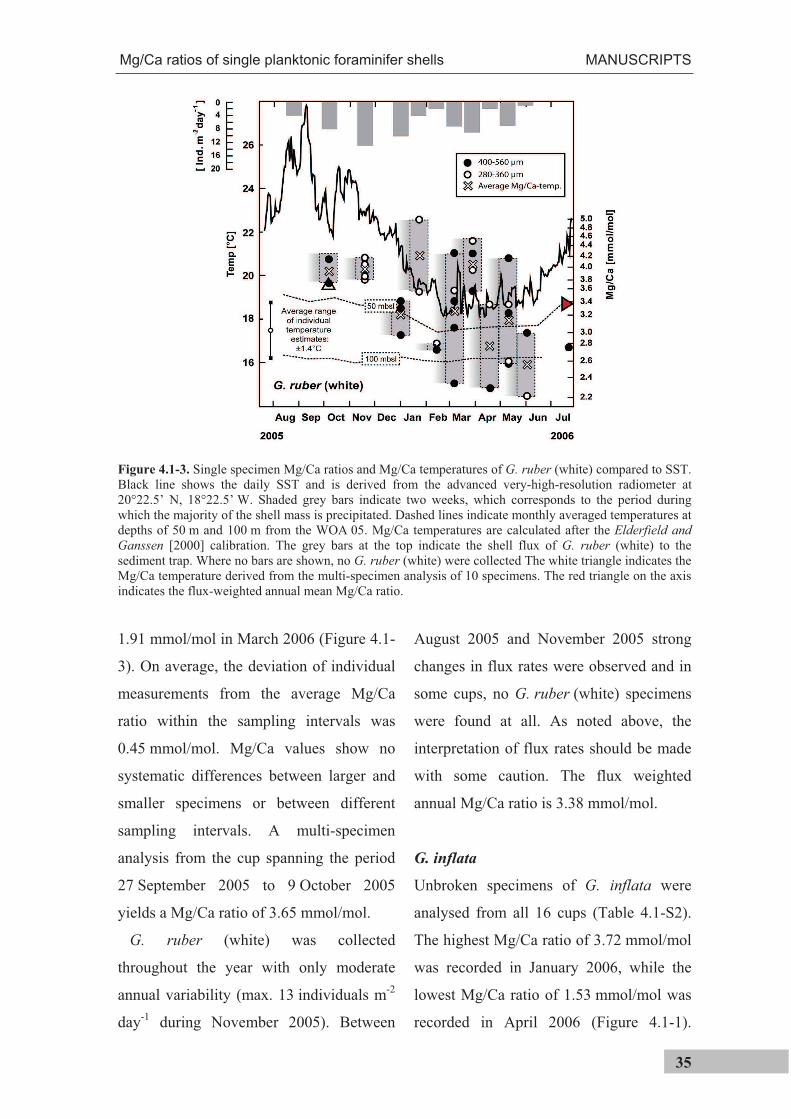
Mg/Ca ratios of single planktonic foraminifer shells MANUSCRIPTS
35
Figure 4.1-3. Single specimen Mg/Ca ratios and Mg/Ca temperatures of G. ruber (white) compared to SST. Black line shows the daily SST and is derived from the advanced very-high-resolution radiometer at 20°22.5’ N, 18°22.5’ W. Shaded grey bars indicate two weeks, which corresponds to the period during which the majority of the shell mass is precipitated. Dashed lines indicate monthly averaged temperatures at depths of 50 m and 100 m from the WOA 05. Mg/Ca temperatures are calculated after the Elderfield and Ganssen [2000] calibration. The grey bars at the top indicate the shell flux of G. ruber (white) to the sediment trap. Where no bars are shown, no G. ruber (white) were collected The white triangle indicates the Mg/Ca temperature derived from the multi-specimen analysis of 10 specimens. The red triangle on the axis indicates the flux-weighted annual mean Mg/Ca ratio.
1.91 mmol/mol in March 2006 (Figure 4.1-
3). On average, the deviation of individual
measurements from the average Mg/Ca
ratio within the sampling intervals was
0.45 mmol/mol. Mg/Ca values show no
systematic differences between larger and
smaller specimens or between different
sampling intervals. A multi-specimen
analysis from the cup spanning the period
27 September 2005 to 9 October 2005
yields a Mg/Ca ratio of 3.65 mmol/mol.
G. ruber (white) was collected
throughout the year with only moderate
annual variability (max. 13 individuals m-2
day-1 during November 2005). Between
August 2005 and November 2005 strong
changes in flux rates were observed and in
some cups, no G. ruber (white) specimens
were found at all. As noted above, the
interpretation of flux rates should be made
with some caution. The flux weighted
annual Mg/Ca ratio is 3.38 mmol/mol.
G. inflata
Unbroken specimens of G. inflata were
analysed from all 16 cups (Table 4.1-S2).
The highest Mg/Ca ratio of 3.72 mmol/mol
was recorded in January 2006, while the
lowest Mg/Ca ratio of 1.53 mmol/mol was
recorded in April 2006 (Figure 4.1-1).
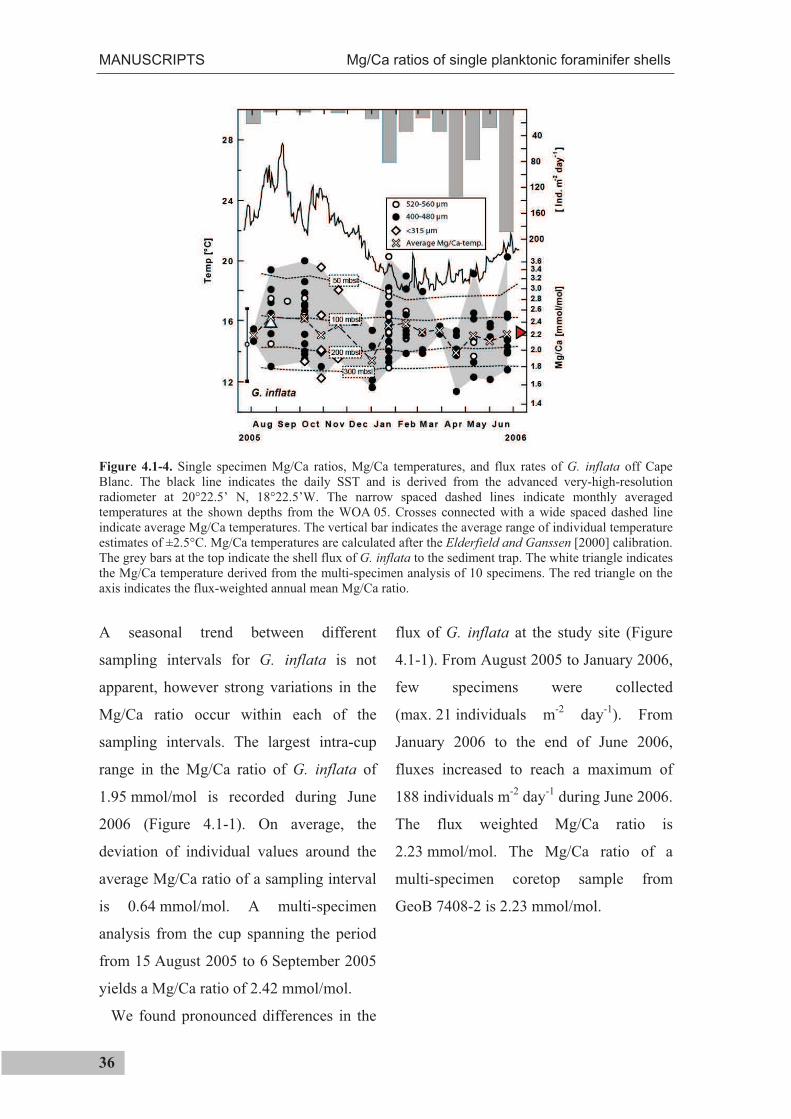
MANUSCRIPTS Mg/Ca ratios of single planktonic foraminifer shells
36
Figure 4.1-4. Single specimen Mg/Ca ratios, Mg/Ca temperatures, and flux rates of G. inflata off Cape Blanc. The black line indicates the daily SST and is derived from the advanced very-high-resolution radiometer at 20°22.5’ N, 18°22.5’W. The narrow spaced dashed lines indicate monthly averaged temperatures at the shown depths from the WOA 05. Crosses connected with a wide spaced dashed line indicate average Mg/Ca temperatures. The vertical bar indicates the average range of individual temperature estimates of ±2.5°C. Mg/Ca temperatures are calculated after the Elderfield and Ganssen [2000] calibration. The grey bars at the top indicate the shell flux of G. inflata to the sediment trap. The white triangle indicates the Mg/Ca temperature derived from the multi-specimen analysis of 10 specimens. The red triangle on the axis indicates the flux-weighted annual mean Mg/Ca ratio.
A seasonal trend between different
sampling intervals for G. inflata is not
apparent, however strong variations in the
Mg/Ca ratio occur within each of the
sampling intervals. The largest intra-cup
range in the Mg/Ca ratio of G. inflata of
1.95 mmol/mol is recorded during June
2006 (Figure 4.1-1). On average, the
deviation of individual values around the
average Mg/Ca ratio of a sampling interval
is 0.64 mmol/mol. A multi-specimen
analysis from the cup spanning the period
from 15 August 2005 to 6 September 2005
yields a Mg/Ca ratio of 2.42 mmol/mol.
We found pronounced differences in the
flux of G. inflata at the study site (Figure
4.1-1). From August 2005 to January 2006,
few specimens were collected
(max. 21 individuals m-2 day-1). From
January 2006 to the end of June 2006,
fluxes increased to reach a maximum of
188 individuals m-2 day-1 during June 2006.
The flux weighted Mg/Ca ratio is
2.23 mmol/mol. The Mg/Ca ratio of a
multi-specimen coretop sample from
GeoB 7408-2 is 2.23 mmol/mol.
Mg/Ca ratios of single planktonic foraminifer shells MANUSCRIPTS
37
4.1.5 Discussion
Seasonal shell abundance
G. ruber (pink) and G. ruber (white) were
collected throughout the year (Figure 4.1-2
and Figure 4.1-3). Fluxes of both species
were very variable. Higher fluxes between
August 2005 and January 2006 were found
for both species, however this is more
pronounced for G. ruber (pink) than for G.
ruber (white). Fluxes of G. inflata between
January 2006 and June 2006 were much
higher than and nearly a mirror-image of
the fluxes of G. ruber (pink). The
differences in abundance are assumed to
result from the exceptional seasonal
changes in the study area. In the upper
water column, these changes are controlled
by large differences in SST. The large
Cape Blanc upwelling filament is also
important. In September 2005, the filament
moved right over the sediment trap (Figure
4.1-1), with high nutrient concentrations at
the surface evident by high chlorophyll a
concentrations. Conversely, in March
2006, the filament was absent in the study
area (Figure 4.1-1). Water temperatures,
the thermal stratification of the water
column and nutrient availability are likely
to act in concert to control shell fluxes at
the study site.
G. ruber (pink) was most abundant
during summer/fall with warm sea surface
temperatures. This is in agreement with the
study of Wilke et al. [2009] who showed
that G. ruber (pink) is most abundant when
surface mixed layer temperatures are
higher than 20°C. Additionally, the strong
thermal stratification during the summer
has been reported to favor G. ruber
[Sautter and Sancetta, 1992]. High nutrient
levels evident by high chlorophyll a
concentrations (Figure 4.1-1) are also
expected to favor the development of
G. ruber (pink).
In contrast, G. inflata flux rates were
lowest between August 2005 and January
2006. Since G. inflata records very similar
Mg/Ca temperatures throughout the year,
water temperatures are expected to play a
minor, if any, role in controlling flux rates.
It is assumed that nutrient availability
controls flux rates of G. inflata in the study
area. CTD casts show that the maximum
chlorophyll a concentration at different
seasons is found above 50 mbsl (Figure
4.1-S1). It is suggested that G. inflata
cannot make use of the high nutrient
concentrations during times of a well
stratified water column in summer.
Contrastingly, during the main upwelling
season in winter/spring, G. inflata is more
suited to the low nutrient concentrations
(Figure 4.1-1) than G. ruber (pink and
white).
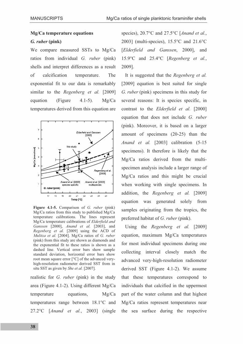
MANUSCRIPTS Mg/Ca ratios of single planktonic foraminifer shells
38
Figure 4.1-5. Comparison of G. ruber (pink) Mg/Ca ratios from this study to published Mg/Ca temperature calibrations. The lines represent Mg/Ca temperature calibrations of Elderfield and Ganssen [2000], Anand et al. [2003], and Regenberg et al. [2009] using the ACD of Mulitza et al. [2004]. Mg/Ca ratios of G. ruber (pink) from this study are shown as diamonds and the exponential fit to these ratios is shown as a dashed line. Vertical error bars show sample standard deviation, horizontal error bars show root mean square error [°C] of the advanced very-high-resolution radiometer derived SST from in situ SST as given by She et al. [2007].
Mg/Ca temperature equations
G. ruber (pink)
We compare measured SSTs to Mg/Ca
ratios from individual G. ruber (pink)
shells and interpret differences as a result
of calcification temperature. The
exponential fit to our data is remarkably
similar to the Regenberg et al. [2009]
equation (Figure 4.1-5). Mg/Ca
temperatures derived from this equation are
realistic for G. ruber (pink) in the study
area (Figure 4.1-2). Using different Mg/Ca
temperature equations, Mg/Ca
temperatures range between 18.1°C and
27.2°C [Anand et al., 2003] (single
species), 20.7°C and 27.5°C [Anand et al.,
2003] (multi-species), 15.5°C and 21.6°C
[Elderfield and Ganssen, 2000], and
15.9°C and 25.4°C [Regenberg et al.,
2009].
It is suggested that the Regenberg et al.
[2009] equation is best suited for single
G. ruber (pink) specimens in this study for
several reasons: It is species specific, in
contrast to the Elderfield et al. [2000]
equation that does not include G. ruber
(pink). Moreover, it is based on a larger
amount of specimens (20-25) than the
Anand et al. [2003] calibration (5-15
specimens). It therefore is likely that the
Mg/Ca ratios derived from the multi-
specimen analysis include a larger range of
Mg/Ca ratios and this might be crucial
when working with single specimens. In
addition, the Regenberg et al. [2009]
equation was generated solely from
samples originating from the tropics, the
preferred habitat of G. ruber (pink).
Using the Regenberg et al. [2009]
equation, maximum Mg/Ca temperatures
for most individual specimens during one
collecting interval closely match the
advanced very-high-resolution radiometer
derived SST (Figure 4.1-2). We assume
that these temperatures correspond to
individuals that calcified in the uppermost
part of the water column and that highest
Mg/Ca ratios represent temperatures near
the sea surface during the respective
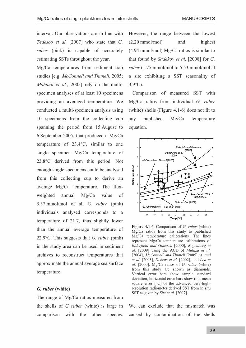
Mg/Ca ratios of single planktonic foraminifer shells MANUSCRIPTS
39
Figure 4.1-6. Comparison of G. ruber (white) Mg/Ca ratios from this study to published Mg/Ca temperature calibrations. The lines represent Mg/Ca temperature calibrations of Elderfield and Ganssen [2000], Regenberg et al. [2009] using the ACD of Mulitza et al.[2004], McConnell and Thunell [2005], Anand et al. [2003], Dekens et al. [2002], and Lea et al. [2000]. Mg/Ca ratios of G. ruber (white) from this study are shown as diamonds. Vertical error bars show sample standard deviation, horizontal error bars show root mean square error [°C] of the advanced very-high-resolution radiometer derived SST from in situ SST as given by She et al. [2007].
interval. Our observations are in line with
Tedesco et al. [2007] who state that G.
ruber (pink) is capable of accurately
estimating SSTs throughout the year.
Mg/Ca temperatures from sediment trap
studies [e.g. McConnell and Thunell, 2005;
Mohtadi et al., 2005] rely on the multi-
specimen analyses of at least 10 specimens
providing an averaged temperature. We
conducted a multi-specimen analysis using
10 specimens from the collecting cup
spanning the period from 15 August to
6 September 2005, that produced a Mg/Ca
temperature of 23.4°C, similar to one
single specimen Mg/Ca temperature of
23.8°C derived from this period. Not
enough single specimens could be analysed
from this collecting cup to derive an
average Mg/Ca temperature. The flux-
weighted annual Mg/Ca value of
3.57 mmol/mol of all G. ruber (pink)
individuals analysed corresponds to a
temperature of 21.7, thus slightly lower
than the annual average temperature of
22.9°C. This suggests that G. ruber (pink)
in the study area can be used in sediment
archives to reconstruct temperatures that
approximate the annual average sea surface
temperature.
G. ruber (white)
The range of Mg/Ca ratios measured from
the shells of G. ruber (white) is large in
comparison with the other species.
However, the range between the lowest
(2.20 mmol/mol) and highest
(4.94 mmol/mol) Mg/Ca ratios is similar to
that found by Sadekov et al. [2008] for G.
ruber (1.75 mmol/mol to 5.53 mmol/mol at
a site exhibiting a SST seasonality of
3.9°C).
Comparison of measured SST with
Mg/Ca ratios from individual G. ruber
(white) shells (Figure 4.1-6) does not fit to
any published Mg/Ca temperature
equation.
We can exclude that the mismatch was
caused by contamination of the shells
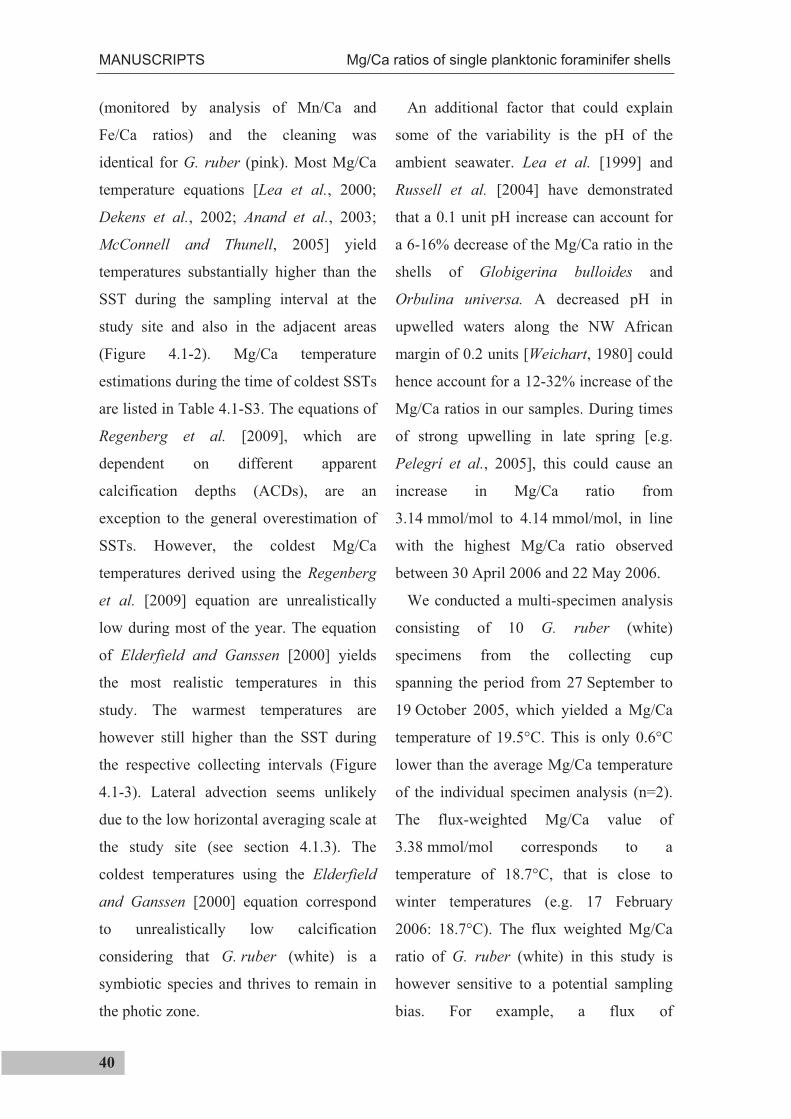
MANUSCRIPTS Mg/Ca ratios of single planktonic foraminifer shells
40
(monitored by analysis of Mn/Ca and
Fe/Ca ratios) and the cleaning was
identical for G. ruber (pink). Most Mg/Ca
temperature equations [Lea et al., 2000;
Dekens et al., 2002; Anand et al., 2003;
McConnell and Thunell, 2005] yield
temperatures substantially higher than the
SST during the sampling interval at the
study site and also in the adjacent areas
(Figure 4.1-2). Mg/Ca temperature
estimations during the time of coldest SSTs
are listed in Table 4.1-S3. The equations of
Regenberg et al. [2009], which are
dependent on different apparent
calcification depths (ACDs), are an
exception to the general overestimation of
SSTs. However, the coldest Mg/Ca
temperatures derived using the Regenberg
et al. [2009] equation are unrealistically
low during most of the year. The equation
of Elderfield and Ganssen [2000] yields
the most realistic temperatures in this
study. The warmest temperatures are
however still higher than the SST during
the respective collecting intervals (Figure
4.1-3). Lateral advection seems unlikely
due to the low horizontal averaging scale at
the study site (see section 4.1.3). The
coldest temperatures using the Elderfield
and Ganssen [2000] equation correspond
to unrealistically low calcification
considering that G. ruber (white) is a
symbiotic species and thrives to remain in
the photic zone.
An additional factor that could explain
some of the variability is the pH of the
ambient seawater. Lea et al. [1999] and
Russell et al. [2004] have demonstrated
that a 0.1 unit pH increase can account for
a 6-16% decrease of the Mg/Ca ratio in the
shells of Globigerina bulloides and
Orbulina universa. A decreased pH in
upwelled waters along the NW African
margin of 0.2 units [Weichart, 1980] could
hence account for a 12-32% increase of the
Mg/Ca ratios in our samples. During times
of strong upwelling in late spring [e.g.
Pelegrí et al., 2005], this could cause an
increase in Mg/Ca ratio from
3.14 mmol/mol to 4.14 mmol/mol, in line
with the highest Mg/Ca ratio observed
between 30 April 2006 and 22 May 2006.
We conducted a multi-specimen analysis
consisting of 10 G. ruber (white)
specimens from the collecting cup
spanning the period from 27 September to
19 October 2005, which yielded a Mg/Ca
temperature of 19.5°C. This is only 0.6°C
lower than the average Mg/Ca temperature
of the individual specimen analysis (n=2).
The flux-weighted Mg/Ca value of
3.38 mmol/mol corresponds to a
temperature of 18.7°C, that is close to
winter temperatures (e.g. 17 February
2006: 18.7°C). The flux weighted Mg/Ca
ratio of G. ruber (white) in this study is
however sensitive to a potential sampling
bias. For example, a flux of
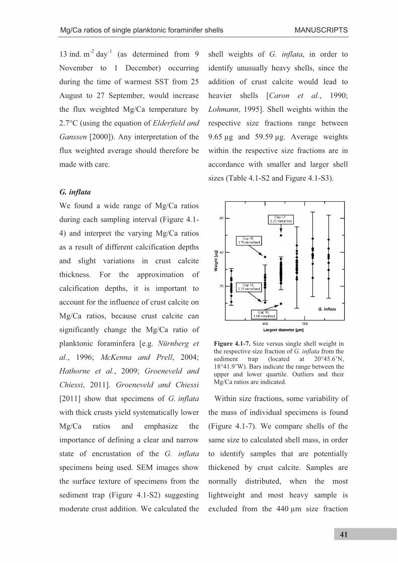
Mg/Ca ratios of single planktonic foraminifer shells MANUSCRIPTS
41
Figure 4.1-7. Size versus single shell weight in the respective size fraction of G. inflata from the sediment trap (located at 20°45.6’N, 18°41.9’W). Bars indicate the range between the upper and lower quartile. Outliers and their Mg/Ca ratios are indicated.
13 ind. m-2 day-1 (as determined from 9
November to 1 December) occurring
during the time of warmest SST from 25
August to 27 September, would increase
the flux weighted Mg/Ca temperature by
2.7°C (using the equation of Elderfield and
Ganssen [2000]). Any interpretation of the
flux weighted average should therefore be
made with care.
G. inflata
We found a wide range of Mg/Ca ratios
during each sampling interval (Figure 4.1-
4) and interpret the varying Mg/Ca ratios
as a result of different calcification depths
and slight variations in crust calcite
thickness. For the approximation of
calcification depths, it is important to
account for the influence of crust calcite on
Mg/Ca ratios, because crust calcite can
significantly change the Mg/Ca ratio of
planktonic foraminfera [e.g. Nürnberg et
al., 1996; McKenna and Prell, 2004;
Hathorne et al., 2009; Groeneveld and
Chiessi, 2011]. Groeneveld and Chiessi
[2011] show that specimens of G. inflata
with thick crusts yield systematically lower
Mg/Ca ratios and emphasize the
importance of defining a clear and narrow
state of encrustation of the G. inflata
specimens being used. SEM images show
the surface texture of specimens from the
sediment trap (Figure 4.1-S2) suggesting
moderate crust addition. We calculated the
shell weights of G. inflata, in order to
identify unusually heavy shells, since the
addition of crust calcite would lead to
heavier shells [Caron et al., 1990;
Lohmann, 1995]. Shell weights within the
respective size fractions range between
9.65 µg and 59.59 µg. Average weights
within the respective size fractions are in
accordance with smaller and larger shell
sizes (Table 4.1-S2 and Figure 4.1-S3).
Within size fractions, some variability of
the mass of individual specimens is found
(Figure 4.1-7). We compare shells of the
same size to calculated shell mass, in order
to identify samples that are potentially
thickened by crust calcite. Samples are
normally distributed, when the most
lightweight and most heavy sample is
excluded from the 440 µm size fraction
MANUSCRIPTS Mg/Ca ratios of single planktonic foraminifer shells
42
Figure 4.1-8. Weight versus single shell Mg/Ca ratios of G. inflata from the sediment trap (located at 20°45.6’N, 18°41.9’W). Outliers and their Mg/Ca ratios are indicated.
(Shapiro-Wilk tested at a 95% level of
confidence). Four outliers can be
identified. The lightest and heaviest
samples from the 440 µm size fraction
deviate from a normal distribution.
Moreover the lightest and heaviest samples
from the 400 µm size fraction are outside
the upper and lower quartiles. The Mg/Ca
ratios of these outliers are however not
noticeably different from all other
specimens (Figure 4.1-8). We therefore
conclude that there is no simple
relationship between the amount of crust
calcite and the Mg/Ca ratios of G. inflata in
this study.
Many studies have recognized the
potential of G. inflata for temperature
reconstructions at the base of the seasonal
thermocline [e.g. Thornalley et al., 2009]
but the existing temperature equations for
this species differ substantially from each
other [Elderfield and Ganssen, 2000;
Anand et al., 2003; Cléroux et al., 2008;
Thornalley et al., 2009; Farmer et al.,
2010; Groeneveld and Chiessi, 2011].
Calculation of Mg/Ca temperatures for G.
inflata using the equations listed in Table
4.1-S1 yields temperature estimates that
are either too warm or too cold when
compared to World Ocean Atlas
temperatures [Locarnini et al., 2006]. In
Table 4.1-S4, we compare Mg/Ca
temperature estimates from individual G.
inflata specimens collected between 27
September and 19 October 2005 to
monthly average World Ocean Atlas water
column temperatures during October
[Locarnini et al., 2006]. The equations of
Anand et al. [2003], Cléroux et al. [2008],
and Farmer et al. [2010] yield warmest
temperatures that are 5.4°C, 6.8°C, and
13.0°C above the observed SST in the
middle of the collecting period. In contrast,
the equations of Elderfield and Ganssen
[2000], Thornalley et al. [2009], and
Groeneveld and Chiessi [2011] yield
temperature estimates that fit with the
water column observations.
A multi-specimen analysis of 10 G.
inflata specimens from the collecting cup
spanning the period from 15 August to
6 September 2005, yields a Mg/Ca
temperature of 16.0°C, similar to the
average Mg/Ca temperature of 16.3°C
Mg/Ca ratios of single planktonic foraminifer shells MANUSCRIPTS
43
from the individual specimen analyses. The
close match of the average temperature
derived from the multi-specimen analysis
and the analyses of single specimens
confirms the excellent potential of our
approach to measure single specimens, in
order to gain information about the overall
variability in Mg/Ca temperatures within a
population.
The average Mg/Ca temperature of G.
inflata from the sediment trap samples
reflects an annual mean temperature at a
depth of about 150 m in the study area
(Figure 4.1-1). The largest deviations from
the average Mg/Ca temperature are
measured in August 2005 (+1.1°C) and
December (-1.8°C). As these periods
coincide with times of low flux, they are
unlikely to lead to a seasonal bias in the
sedimentary record. This is supported by
the multi-specimen analysis of G. inflata
from coretop GeoB7408-2, which yields a
Mg/Ca ratio of 2.23 mmol/mol. The
average Mg/Ca ratio of all G. inflata
samples from the sediment trap is between
2.23 mmol/mol and 2.38 mmol/mol at a
confidence level of 95% and the flux-
weighted average is also 2.23 mmol/mol.
The good match with the multi-specimen
analysis from the sedimentary record
supports the assumption that there is no
seasonal bias in the Mg/Ca signal of G.
inflata.
Comparison of inferred calcification
depths to reported habitat depths from
plankton tows
The Mg/Ca temperature estimates derived
using the Regenberg et al. [2009] equation
mostly correspond to a calcification depth
for G. ruber (pink) between the surface and
~30 m. This is within the mixed layer at a
habitat depth reported in tow studies for
this species [e.g. Wilke et al., 2009]. An
exception is the lowest temperature
(15.9°C) recorded in February 2006
(Figure 4.1-2). Though very low, we
assume that this temperature is a realistic
record of the calcification temperature at
the study site, due to the low horizontal
averaging scale at the study site (see
section 4.1.3). One possibility could be that
the specimen calcified within the upwelled
water. Everywhere along the NW African
coast, this has a temperature of 15 - 17°C
[Mittelstaedt, 1983].
Mg/Ca temperatures recorded by G.
ruber (white) using the Elderfield and
Ganssen [2000] equation correspond to
calcification depths between the surface
and ~40 m (October 2005), 0 m (January
2006), ~110 m (February 2006), and
~150 m (May 2006) when compared to
World Ocean Atlas data (Figure 4.1-3;
Locarnini et al., 2006). It is difficult to
reconcile these calcification depths given
the fact that G. ruber (white) has symbiotic
dinoflagellates and should be restricted to
MANUSCRIPTS Mg/Ca ratios of single planktonic foraminifer shells
44
the photic zone. As noted above the
calcification depths for G. ruber (white)
should be treated with caution.
Calculated apparent calcification depths
of G. inflata mostly correspond to the
upper 400 m [Elderfield and Ganssen,
2000 equation], 500 m [Groeneveld and
Chiessi, 2011 equation], and 75 to 500 m
[Thornalley et al., 2009 equation] of the
water column. In this study, we use the
Elderfield and Ganssen [2000] equation
generated using North Atlantic sediment
samples. When compared to World Ocean
Atlas data, the majority of our data indicate
a shallowest apparent calcification depth
between the sea surface and 50 m, hence at
the depth of the highest chlorophyll a
concentration (Figure 4.1-S1), where
G. inflata can make use of its food source.
The mean temperature estimates of the
individual sampling intervals are between
16.3°C and 13.4°C, corresponding to
calcification depths between about 100 m
and 300 m, respectively, hence well below
the seasonal thermocline which is at ~
50 m (Figure 4.1-S1). The interpretation of
this large range of calculated calcification
depths must account for G. inflata
calcifying over a wide range of depths,
reflected in the depth integrated
composition of its shell [Wilke et al.,
2006]. It builds part of its shell in the
surface mixed layer and the thermocline
[Wilke et al., 2006]. The fact that G. inflata
has small symbiotic algae [Gastrich et al.,
1987] suggests that it spends part of the life
cycle in the photic zone. However, wall
thickening at depth produces crust calcite
with a lower Mg/Ca ratio that can
constitute a large proportion of the final
test mass. This means that apparent
calcification depths can be deeper than the
depth at which the individuals spent most
of their lives.
Implications for paleoceanographic
reconstructions
Based on the distribution of single
specimen Mg/Ca ratios of G. ruber (white),
G. ruber (pink) and G. inflata, it is
suggested that in the study area, G. ruber
(pink) is suitable for investigations of
paleo-seasonality. In contrast, G. ruber
(white) does not appear to be applicable for
this purpose in the study area using
published Mg/Ca temperature equations.
The inferred apparent calcification depth of
G. inflata below the depth of the seasonal
thermocline suggests this species is a
recorder of subsurface temperatures.
Changes in single specimen maximum and
minimum calcification temperatures from
sediment core samples could indicate
calcification at different subsurface depths
in the past.
A study on single specimens of
planktonic foraminifera by Billups and
Spero [1996] demonstrates that the range
Mg/Ca ratios of single planktonic foraminifer shells MANUSCRIPTS
45
of 18O values can be used in order to
assess seasonal or depth-related
calcification temperatures in the
paleoceanographic past. Koutavas et al.
[2006] show that a change in total variance
between populations of planktonic
foraminifera (G. ruber (white)) can provide
information on ENSO and seasonal
variability. Accordingly, we suggest that a
change in Mg/Ca variance and Mg/Ca
range can be used as an indicator for
environmental variability in the study area
when measured on downcore samples.
G. ruber (pink)
The present day difference between highest
and lowest Mg/Ca ratios of single G. ruber
(pink) specimens in the study area over an
annual cycle is 2.08 mmol/mol (Table 4.1-
S2), corresponding to the difference
between warmest and coldest temperatures
under which the specimens calcified
(Figure 4.1-2). Likewise in the sedimentary
record, the difference between highest and
lowest Mg/Ca ratios is expected to indicate
the range of temperatures under which the
specimens calcified. It is suggested that
changes in the range between highest and
lowest Mg/Ca ratios in the sedimentary
record are a measure of interannual
changes in the range between highest and
lowest SST. A prerequisite for such
interpretation is that potential artifacts
introduced by variable sedimentation rate
and bioturbation can be minimized and
natural variability can be confined.
The annual Mg/Ca variance of G. ruber
(pink) in this study is 1.43 mmol/mol and
the 95% confidence interval of this
variance ranges from 0.88 mmol/mol to
2.73 mmol/mol. This means that when a
different variance measured from
sedimentary specimens (with its own
confidence interval) falls outside this
estimate, it would be significantly different
from the variance of the sample
investigated here. A hypothetical decrease
of variance below this threshold of
0.88 mmol/mol would mean a decrease of
variance by 38%. If we assume that the
variance relative to the total range of
values remains the same (69%) in the past
in the study area, a significant decrease of
the total variance (below 0.88 mmol/mol)
requires a decrease of the Mg/Ca range
from 2.08 mmol/mol to 1.28 mmol/mol.
Using the equation of Regenberg et al.
[2009], this would represent a decrease in
the temperature range of 4.0°C, from
10.0°C to 6.0°C. We did not calculate what
increase in the temperature range would be
significant as the modern range is already
large (10°C) and a substantial increase is
rather unlikely.
G. inflata
The annual variance of G. inflata in this
study is 1.37 mmol/mol and the 95%
MANUSCRIPTS Mg/Ca ratios of single planktonic foraminifer shells
46
confidence interval of this variance ranges
from 1.08 mmol/mol to 1.80 mmol/mol.
Again, a variance of sedimentary
specimens that falls outside of this
confidence interval would be significantly
different from the samples investigated
here. A decrease of variance beyond the
significance threshold of 1.08 mmol/mol
would mean a decrease of variance by
21%. If we again hypothesize that the
variance relative to the total range of
values remains the same (85%) in the study
area throughout the past, a significant
decrease of the total variance below the
significance threshold of 1.08 mmol/mol
requires a decrease of the total Mg/Ca
range from 1.62 mmol/mol to
1.28 mmol/mol. Using the equation of
Elderfield and Ganssen [2000], this would
represent a decrease in the temperature
range of 1.7°C, from 7.6°C to 5.9°C. A
reduction of the temperature range of this
magnitude was shown by Billups and
Spero [1996] for the western equatorial
Atlantic using individual
Neogloboquadrina dutertrei shells.
N. dutertrei is a species that prefers
oceanographic conditions similar to
G. inflata, i.e. upwelling regions and a
habitat close to the chlorophyll maximum
at the bottom of the mixed layer
[Fairbanks et al., 1982]. Between isotopic
stage 1 and 2, a decrease of the temperature
range of 4.7°C in the western equatorial
Atlantic was suggested Billups and Spero
[1996]. Given the detectable change
(1.7°C) of the temperature range suggested
in our study, the analysis of single
G. inflata could prove valuable for
detecting changes of thermocline
temperatures or calcification depths in the
paleoceanographic past.
4.1.6 Conclusions
Mg/Ca thermometry of single specimens of
G. ruber (pink) is suitable in the upwelling
region off Cape Blanc for tracking the
seasonal amplitude of SST when applying
the Mg/Ca temperature equation of
Regenberg et al. [2009]. In contrast,
Mg/Ca ratios of G. ruber (white) do not
track seasonal SST using published Mg/Ca
temperature equations. The best SST
estimate is obtained when using the
Elderfield and Ganssen [2000] equation.
Mg/Ca ratios of single specimens of G.
inflata do not exhibit any apparent
seasonality and are remarkably similar
throughout the year. The best SST estimate
is also obtained when using the Elderfield
and Ganssen [2000] equation for G.
inflata.
Statistical analysis of single specimen
Mg/Ca ratios from this study suggests that
G. ruber (pink) can serve as potential
recorder of paleo-seasonality in the
sedimentary record. Single specimen
Mg/Ca ratios of G. inflata are suggested to
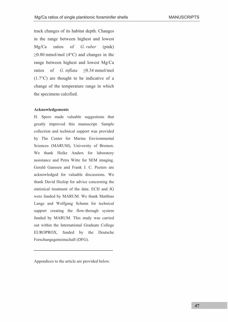
Mg/Ca ratios of single planktonic foraminifer shells MANUSCRIPTS
47
track changes of its habitat depth. Changes
in the range between highest and lowest
Mg/Ca ratios of G. ruber (pink)
0.80 mmol/mol (4°C) and changes in the
range between highest and lowest Mg/Ca
ratios of G. inflata 0.34 mmol/mol
(1.7°C) are thought to be indicative of a
change of the temperature range in which
the specimens calcified.
Acknowledgements
H. Spero made valuable suggestions that
greatly improved this manuscript. Sample
collection and technical support was provided
by The Center for Marine Environmental
Sciences (MARUM), University of Bremen.
We thank Heike Anders for laboratory
assistance and Petra Witte for SEM imaging.
Gerald Ganssen and Frank J. C. Peeters are
acknowledged for valuable discussions. We
thank David Heslop for advice concerning the
statistical treatment of the data. ECH and JG
were funded by MARUM. We thank Matthias
Lange and Wolfgang Schunn for technical
support creating the flow-through system
funded by MARUM. This study was carried
out within the International Graduate College
EUROPROX, funded by the Deutsche
Forschungsgemeinschaft (DFG).
Appendices to the article are provided below.
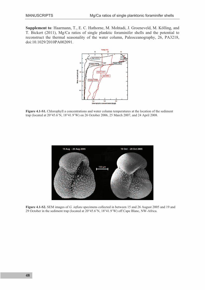
MANUSCRIPTS Mg/Ca ratios of single planktonic foraminifer shells
48
Supplement to: Haarmann, T., E. C. Hathorne, M. Mohtadi, J. Groeneveld, M. Kölling, and T. Bickert (2011), Mg/Ca ratios of single planktic foraminifer shells and the potential to reconstruct the thermal seasonality of the water column, Paleoceanography, 26, PA3218, doi:10.1029/2010PA002091.
Figure 4.1-S1. Chlorophyll a concentrations and water column temperatures at the location of the sediment trap (located at 20°45.6’N, 18°41.9’W) on 26 October 2006, 25 March 2007, and 24 April 2008.
Figure 4.1-S2. SEM images of G. inflata specimens collected in between 15 and 26 August 2005 and 19 and 29 October in the sediment trap (located at 20°45.6’N, 18°41.9’W) off Cape Blanc, NW-Africa.
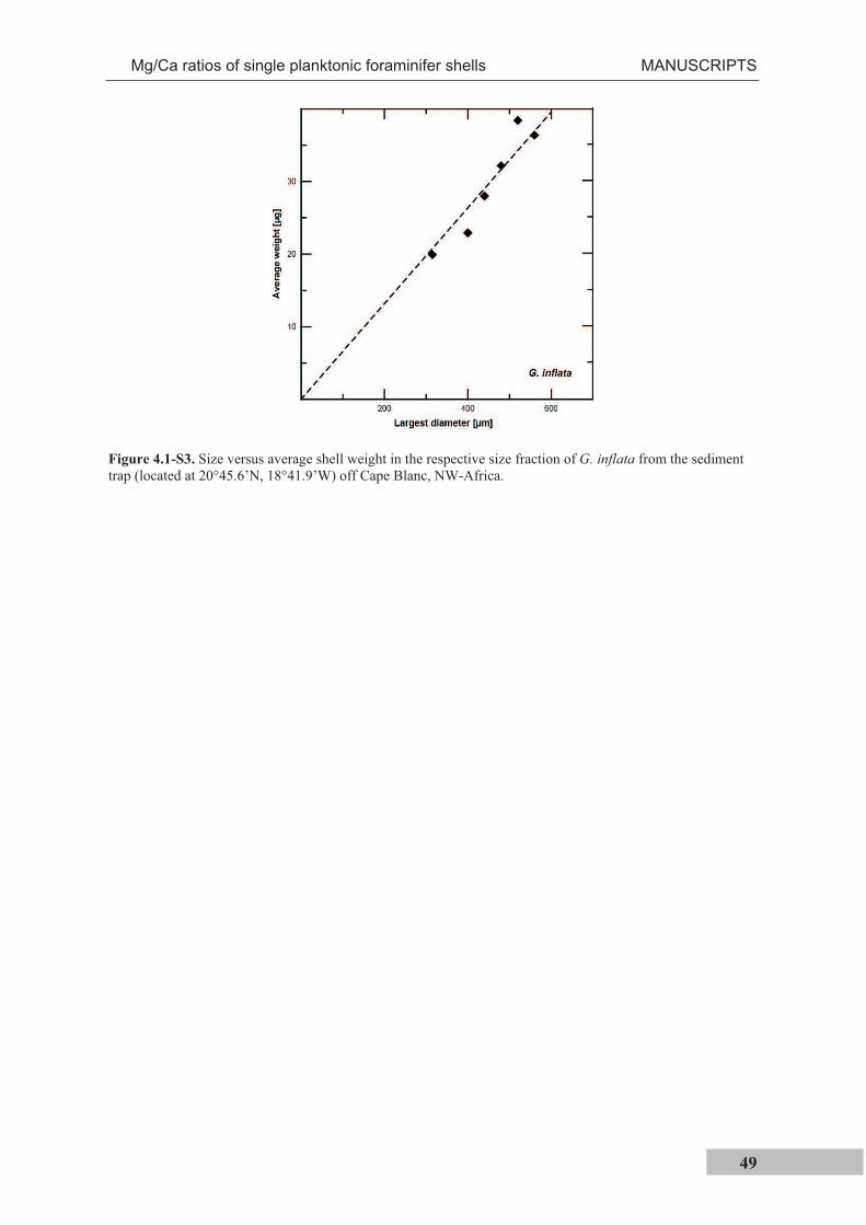
Mg/Ca ratios of single planktonic foraminifer shells MANUSCRIPTS
49
Figure 4.1-S3. Size versus average shell weight in the respective size fraction of G. inflata from the sediment trap (located at 20°45.6’N, 18°41.9’W) off Cape Blanc, NW-Africa.
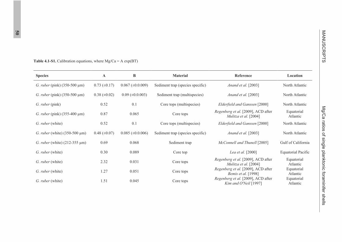
MA
NU
SC
RIP
TS
Mg
/Ca
ratio
s o
f sin
gle
pla
nkto
nic
fora
min
ifer s
he
lls
50
Location
North Atlantic
North Atlantic
North Atlantic
EquatorialAtlantic
North Atlantic
North Atlantic
Gulf of California
Equatorial Pacific
EquatorialAtlantic
EquatorialAtlantic
EquatorialAtlantic
Reference
Anand et al. [2003]
Anand et al. [2003]
Elderfield and Ganssen [2000]
Regenberg et al. [2009], ACD after Mulitza et al. [2004]
Elderfield and Ganssen [2000]
Anand et al. [2003]
McConnell and Thunell [2005]
Lea et al. [2000]
Regenberg et al. [2009], ACD after Mulitza et al. [2004]
Regenberg et al. [2009], ACD after Bemis et al. [1998]
Regenberg et al. [2009], ACD after Kim and O'Neil [1997]
Material
Sediment trap (species specific)
Sediment trap (multispecies)
Core tops (multispecies)
Core tops
Core tops (multispecies)
Sediment trap (species specific)
Sediment trap
Core top
Core tops
Core tops
Core tops
B
0.067 (±0.0.009)
0.09 (±0.0.003)
0.1
0.065
0.1
0.085 (±0.0.006)
0.068
0.089
0.031
0.051
0.045
A
0.73 (±0.17)
0.38 (±0.02)
0.52
0.87
0.52
0.48 (±0.07)
0.69
0.30
2.32
1.27
1.51
Table 4.1-S1. Calibration equations, where Mg/Ca = A exp(BT)
Species
G. ruber (pink) (350-500 µm)
G. ruber (pink) (350-500 µm)
G. ruber (pink)
G. ruber (pink) (355-400 µm)
G. ruber (white)
G. ruber (white) (350-500 µm)
G. ruber (white) (212-355 µm)
G. ruber (white)
G. ruber (white)
G. ruber (white)
G. ruber (white)
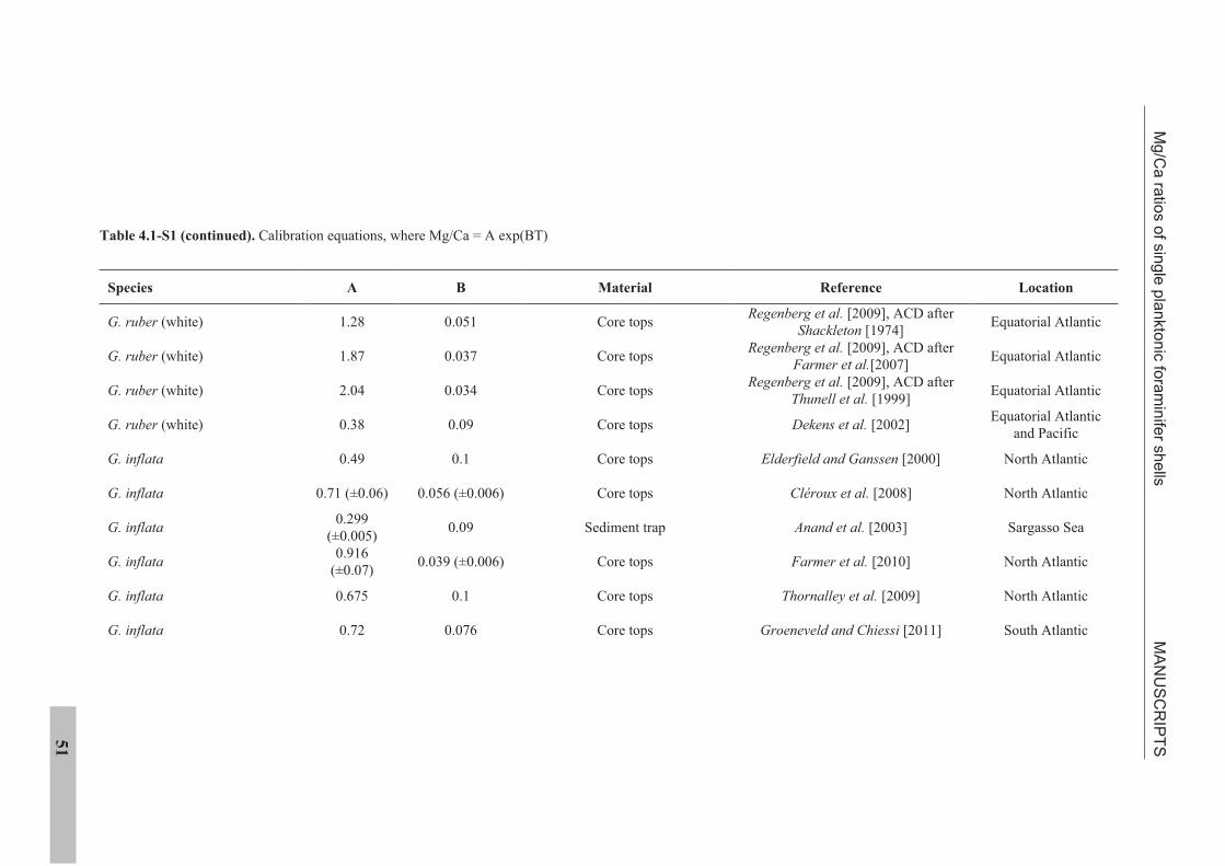
Mg
/Ca
ratio
s o
f sin
gle
pla
nkto
nic
fora
min
ifer s
he
lls M
AN
US
CR
IPT
S
51
Location
Equatorial Atlantic
Equatorial Atlantic
Equatorial Atlantic
Equatorial Atlantic and Pacific
North Atlantic
North Atlantic
Sargasso Sea
North Atlantic
North Atlantic
South Atlantic
Reference
Regenberg et al. [2009], ACD after Shackleton [1974]
Regenberg et al. [2009], ACD after Farmer et al.[2007]
Regenberg et al. [2009], ACD after Thunell et al. [1999]
Dekens et al. [2002]
Elderfield and Ganssen [2000]
Cléroux et al. [2008]
Anand et al. [2003]
Farmer et al. [2010]
Thornalley et al. [2009]
Groeneveld and Chiessi [2011]
Material
Core tops
Core tops
Core tops
Core tops
Core tops
Core tops
Sediment trap
Core tops
Core tops
Core tops
B
0.051
0.037
0.034
0.09
0.1
0.056 (±0.006)
0.09
0.039 (±0.006)
0.1
0.076
A
1.28
1.87
2.04
0.38
0.49
0.71 (±0.06)
0.299 (±0.005)
0.916 (±0.07)
0.675
0.72
Table 4.1-S1 (continued). Calibration equations, where Mg/Ca = A exp(BT)
Species
G. ruber (white)
G. ruber (white)
G. ruber (white)
G. ruber (white)
G. inflata
G. inflata
G. inflata
G. inflata
G. inflata
G. inflata
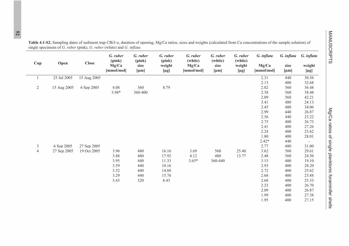
MA
NU
SC
RIP
TS
Mg
/Ca
ratio
s o
f sin
gle
pla
nkto
nic
fora
min
ifer s
he
lls
52
G. inflata
weight
[µg]
30.56 32.68 36.48 38.48 42.21 24.13 34.06 26.87 23.22 26.73 27.26 23.62 28.01
-31.00 29.61 24.50 19.10 28.20 25.62 23.88 25.33 26.70 26.87 27.38 27.15
G. inflata
size
[µm]
440 400 560 560 560 480 480 440 440 400 400 400 400 440 480 560 560 400 400 400 400 400 400 400 400 400
G. inflata
Mg/Ca
[mmol/mol]
2.31 2.13 2.82 2.38 2.09 3.41 2.45 2.99 2.56 2.75 2.41 2.24 1.80
2.42* 2.77 3.62 2.48 3.15 2.93 2.72 2.68 2.68 2.23 2.09 1.99 1.95
G. ruber
(white)
weight
[µg]
25.40 13.77
G. ruber
(white)
size
[µm]
560 480
360-440
G. ruber
(white)
Mg/Ca
[mmol/mol]
3.69 4.12
3.65*
G. ruber
(pink)
weight
[µg]
8.79
16.16 17.92 11.33 10.16 14.88 15.76 8.43
G. ruber
(pink)
size
[µm]
360 360-400
480 480 440 440 440 440 320
G. ruber
(pink)
Mg/Ca
[mmol/mol]
4.08 3.98*
3.96 3.88 3.95 3.59 3.52 3.29 3.43
Close
15 Aug 2005
6 Sep 2005
27 Sep 2005 19 Oct 2005
Open
25 Jul 2005
15 Aug 2005
6 Sep 2005 27 Sep 2005
Table 4.1-S2. Sampling dates of sediment trap CBi3-o, duration of opening, Mg/Ca ratios, sizes and weights (calculated from Ca concentrations of the sample solution) of single specimens of G. ruber (pink), G. ruber (white) and G. inflata
Cup
1
2
34
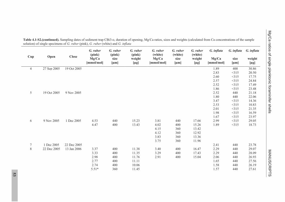
Mg
/Ca
ratio
s o
f sin
gle
pla
nkto
nic
fora
min
ifer s
he
lls M
AN
US
CR
IPT
S
53
G. inflata
weight
[µg]
30.86 20.50 17.75 24.84 17.49 23.48 21.18 22.06 14.36 10.83 21.35 16.59 23.97 29.05 18.73
23.78 29.07 28.09 26.93 27.56 26.19 27.61
G. inflata
size
[µm]
400 <315<315<315<315<315440 440
<315<315<315<315<315<315<315
440 440 440 440 440 440 440
G. inflata
Mg/Ca
[mmol/mol]
1.89 2.83 2.60 2.57 2.52 1.86 2.52 1.80 3.47 2.53 2.01 1.98 1.67 2.99 1.89
2.41 2.29 2.29 2.06 1.65 1.58 1.57
G. ruber
(white)
weight
[µg]
17.66 15.26 13.42 12.92 13.36 11.96
16.47 17.43 15.04
G. ruber
(white)
size
[µm]
440 400 360 360 360 360
400 400 400
G. ruber
(white)
Mg/Ca
[mmol/mol]
3.81 4.02 4.15 4.12 3.83 3.75
3.40 3.29 2.91
G. ruber
(pink)
weight
[µg]
15.23 13.43
11.38 11.35 11.76 11.11 10.06 11.45
G. ruber
(pink)
size
[µm]
440 400
400 400 400 400 400 360
G. ruber
(pink)
Mg/Ca
[mmol/mol]
4.53 4.47
3.37 3.33 2.98 2.77 2.74
5.51*
Close
19 Oct 2005
9 Nov 2005
1 Dec 2005
22 Dec 2005 13 Jan 2006
Open
27 Sep 2005
19 Oct 2005
9 Nov 2005
1 Dec 2005 22 Dec 2005
Table 4.1-S2.(continued). Sampling dates of sediment trap CBi3-o, duration of opening, Mg/Ca ratios, sizes and weights (calculated from Ca concentrations of the sample solution) of single specimens of G. ruber (pink), G. ruber (white) and G. inflata
Cup
4
5
6
78
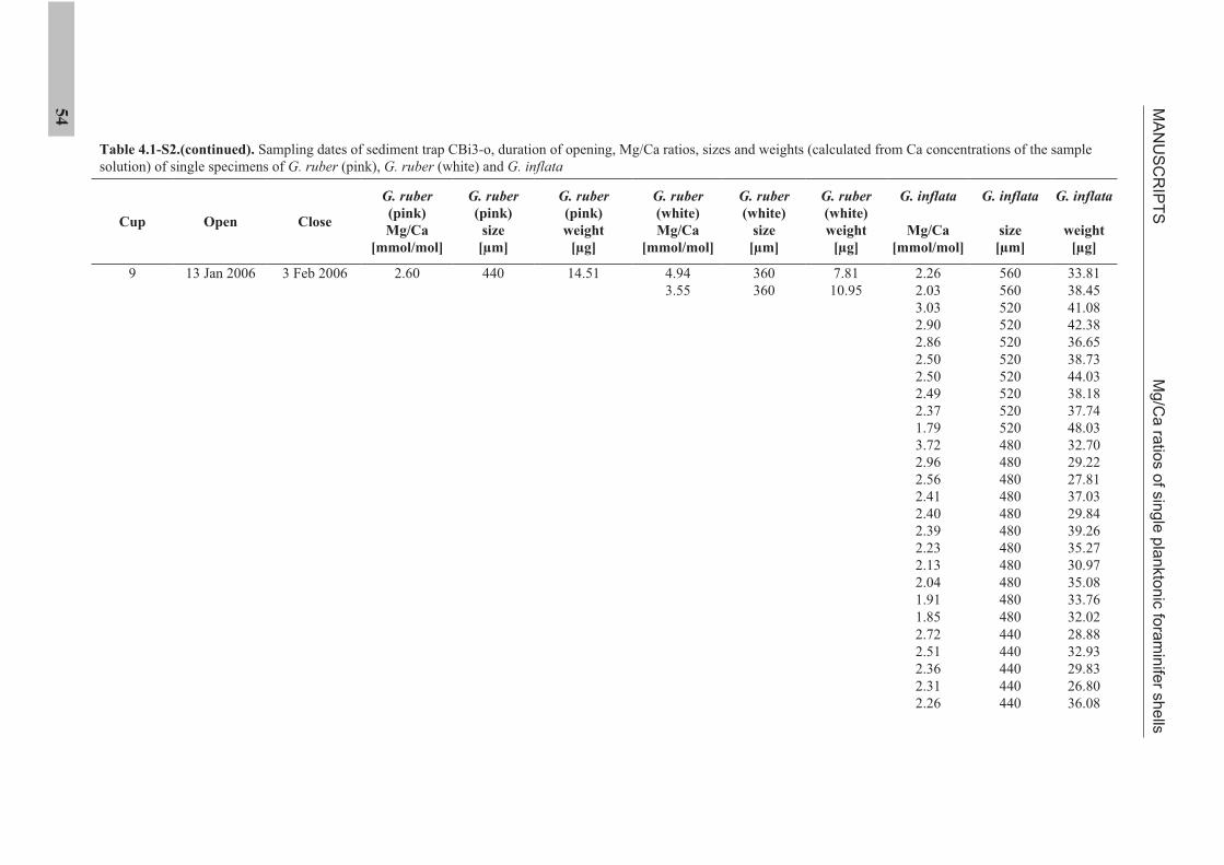
MA
NU
SC
RIP
TS
Mg
/Ca
ratio
s o
f sin
gle
pla
nkto
nic
fora
min
ifer s
he
lls
54
G. inflata
weight
[µg]
33.81 38.45 41.08 42.38 36.65 38.73 44.03 38.18 37.74 48.03 32.70 29.22 27.81 37.03 29.84 39.26 35.27 30.97 35.08 33.76 32.02 28.88 32.93 29.83 26.80 36.08
G. inflata
size
[µm]
560 560 520 520 520 520 520 520 520 520 480 480 480 480 480 480 480 480 480 480 480 440 440 440 440 440
G. inflata
Mg/Ca
[mmol/mol]
2.26 2.03 3.03 2.90 2.86 2.50 2.50 2.49 2.37 1.79 3.72 2.96 2.56 2.41 2.40 2.39 2.23 2.13 2.04 1.91 1.85 2.72 2.51 2.36 2.31 2.26
G. ruber
(white)
weight
[µg]
7.81 10.95
G. ruber
(white)
size
[µm]
360 360
G. ruber
(white)
Mg/Ca
[mmol/mol]
4.94 3.55
G. ruber
(pink)
weight
[µg]
14.51
G. ruber
(pink)
size
[µm]
440
G. ruber
(pink)
Mg/Ca
[mmol/mol]
2.60
Close
3 Feb 2006
Open
13 Jan 2006
Table 4.1-S2.(continued). Sampling dates of sediment trap CBi3-o, duration of opening, Mg/Ca ratios, sizes and weights (calculated from Ca concentrations of the sample solution) of single specimens of G. ruber (pink), G. ruber (white) and G. inflata
Cup
9
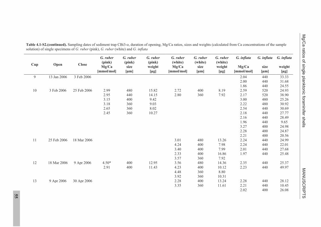
Mg
/Ca
ratio
s o
f sin
gle
pla
nkto
nic
fora
min
ifer s
he
lls M
AN
US
CR
IPT
S
55
G. inflata
weight
[µg]
33.33 31.68 24.55 24.93 38.90 25.26 30.92 30.69 27.77 28.49 9.65
24.98 24.87 20.56 24.99 22.01 27.68 25.48
25.37 49.97
28.12 10.45 26.08
G. inflata
size
[µm]
440 440 440 520 520 480 480 440 440 440 440 400 400 400 440 440 440 440
440 440
440 440 400
G. inflata
Mg/Ca
[mmol/mol]
2.04 2.00 1.86 2.59 2.17 3.00 2.22 2.54 2.18 2.16 1.96 3.27 2.28 2.21 2.24 2.24 2.01 1.97
2.35 2.23
2.28 2.21 2.02
G. ruber
(white)
weight
[µg]
8.19 7.92
13.26 7.98 7.99
16.86 7.92
14.36 10.12 8.80
10.31 13.24 11.61
G. ruber
(white)
size
[µm]
400 360
480 400 400 400 360 480 400 360 360 400 360
G. ruber
(white)
Mg/Ca
[mmol/mol]
2.72 2.80
3.01 4.24 3.40 2.33 3.57 3.56 4.23 4.48 3.92 2.28 3.35
G. ruber
(pink)
weight
[µg]
15.82 14.15 9.42 9.03 8.02 10.27
12.95 11.43
G. ruber
(pink)
size
[µm]
480 440 400 360 360 360
400 400
G. ruber
(pink)
Mg/Ca
[mmol/mol]
2.99 2.95 3.15 3.18 2.65 2.45
4.50* 2.91
Close
3 Feb 2006
25 Feb 2006
18 Mar 2006
9 Apr 2006
30 Apr 2006
Open
13 Jan 2006
3 Feb 2006
25 Feb 2006
18 Mar 2006
9 Apr 2006
Table 4.1-S2.(continued). Sampling dates of sediment trap CBi3-o, duration of opening, Mg/Ca ratios, sizes and weights (calculated from Ca concentrations of the sample solution) of single specimens of G. ruber (pink), G. ruber (white) and G. inflata
Cup
9
10
11
12
13
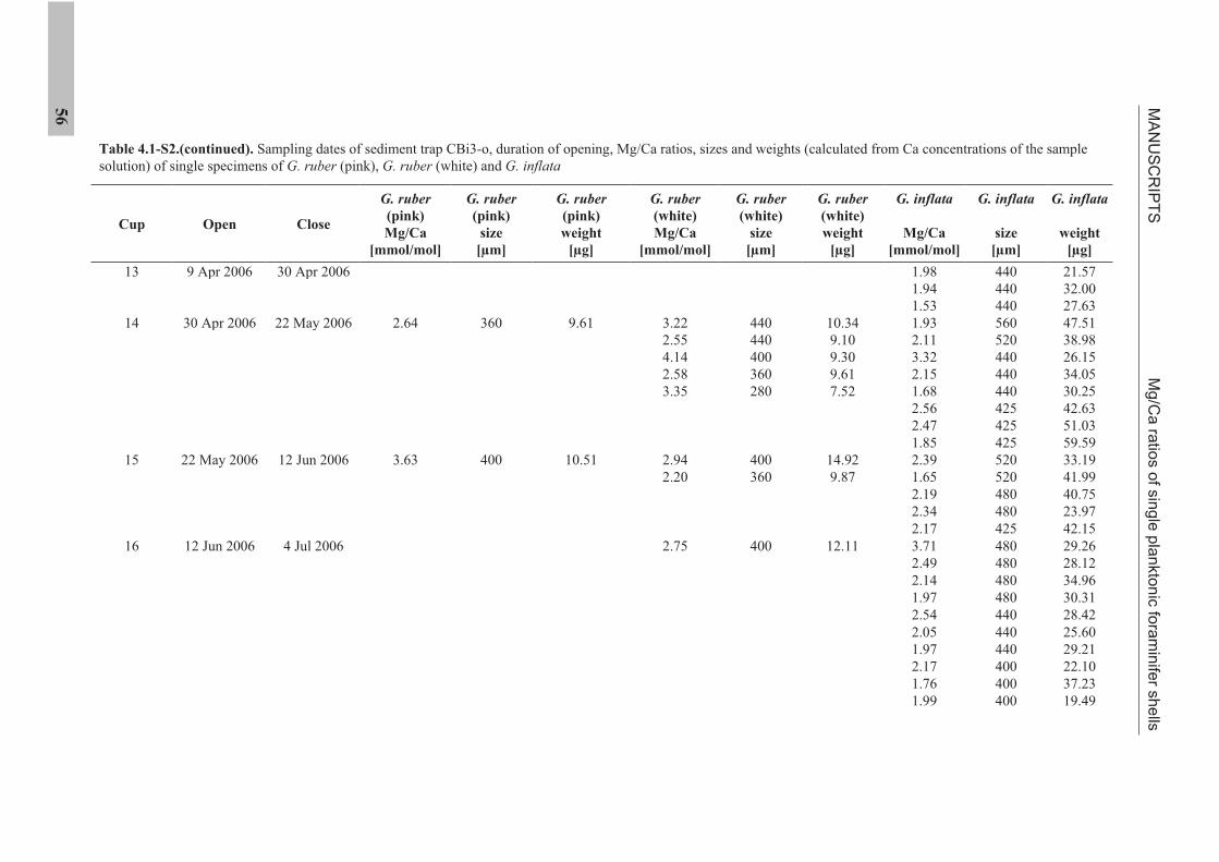
MA
NU
SC
RIP
TS
Mg
/Ca
ratio
s o
f sin
gle
pla
nkto
nic
fora
min
ifer s
he
lls
56
G. inflata
weight
[µg]
21.57 32.00 27.63 47.51 38.98 26.15 34.05 30.25 42.63 51.03 59.59 33.19 41.99 40.75 23.97 42.15 29.26 28.12 34.96 30.31 28.42 25.60 29.21 22.10 37.23 19.49
G. inflata
size
[µm]
440 440 440 560 520 440 440 440 425 425 425 520 520 480 480 425 480 480 480 480 440 440 440 400 400 400
G. inflata
Mg/Ca
[mmol/mol]
1.98 1.94 1.53 1.93 2.11 3.32 2.15 1.68 2.56 2.47 1.85 2.39 1.65 2.19 2.34 2.17 3.71 2.49 2.14 1.97 2.54 2.05 1.97 2.17 1.76 1.99
G. ruber
(white)
weight
[µg]
10.34 9.10 9.30 9.61 7.52
14.92 9.87
12.11
G. ruber
(white)
size
[µm]
440 440 400 360 280
400 360
400
G. ruber
(white)
Mg/Ca
[mmol/mol]
3.22 2.55 4.14 2.58 3.35
2.94 2.20
2.75
G. ruber
(pink)
weight
[µg]
9.61
10.51
G. ruber
(pink)
size
[µm]
360
400
G. ruber
(pink)
Mg/Ca
[mmol/mol]
2.64
3.63
Close
30 Apr 2006
22 May 2006
12 Jun 2006
4 Jul 2006
Open
9 Apr 2006
30 Apr 2006
22 May 2006
12 Jun 2006
Table 4.1-S2.(continued). Sampling dates of sediment trap CBi3-o, duration of opening, Mg/Ca ratios, sizes and weights (calculated from Ca concentrations of the sample solution) of single specimens of G. ruber (pink), G. ruber (white) and G. inflata
Cup
13
14
15
16
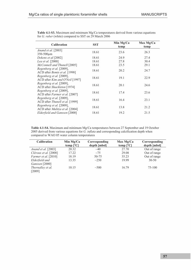
Mg/Ca ratios of single planktonic foraminifer shells MANUSCRIPTS
57
Table 4.1-S3. Maximum and minimum Mg/Ca temperatures derived from various equations for G. ruber (white) compared to SST on 29 March 2006
Calibration SST Min Mg/Ca
temp
Max Mg/Ca
temp
Anand et al. [2003] 350-500µm
18.61 23.6 26.3
Dekens et al [2002] 18.61 24.9 27.4 Lea et al. [2000] 18.61 27.8 30.4 McConnell and Thunell [2005] 18.61 23.5 29.1 Regenberg et al. [2009], ACD after Bemis et al. [1998]
18.61 20.2 24.7
Regenberg et al. [2009], ACD after Kim and O'Neil [1997]
18.61 19.1 22.9
Regenberg et al. [2009], ACD after Shackleton [1974]
18.61 20.1 24.6
Regenberg et al. [2009], ACD after Farmer et al. [2007]
18.61 17.4 23.6
Regenberg et al. [2009], ACD after Thunell et al. [1999]
18.61 16.4 23.1
Regenberg et al. [2009], ACD after Mulitza et al. [2004]
18.61 13.8 21.2
Elderfield and Ganssen [2000] 18.61 19.2 21.5
Table 4.1-S4. Maximum and minimum Mg/Ca temperatures between 27 September and 19 October 2005 derived from various equations for G. inflata and corresponding calcification depth when compared to WAO 05 water column temperatures
Calibration Min Mg/Ca
temp [°C]
Corresponding
depth [mbsl]
Max Mg/Ca
temp [°C]
Corresponding
depth [mbsl]
Anand et al. [2003] 20.32 ~40 27.70 Out of range Cléroux et al. [2008] 17.22 ~75 29.08 Out of range Farmer et al. [2010] 18.19 50-75 35.23 Out of range Elderfield and Ganssen [2000]
13.35 ~250 19.99 30-50
Thornalley et al.[2009]
10.15 ~500 16.79 75-100

58
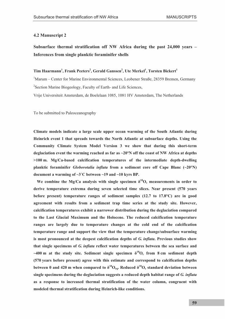
Subsurface thermal stratification off NW Africa MANUSCRIPTS
59
4.2 Manuscript 2
Subsurface thermal stratification off NW Africa during the past 24,000 years –
Inferences from single planktic foraminifer shells
Tim Haarmann1, Frank Peeters
2, Gerald Ganssen
2, Ute Merkel
1, Torsten Bickert
1
1Marum – Center for Marine Environmental Sciences, Leobener Straße, 28359 Bremen, Germany
2Section Marine Biogeology, Faculty of Earth- and Life Sciences,
Vrije Universiteit Amsterdam, de Boelelaan 1085, 1081 HV Amsterdam, The Netherlands
To be submitted to Paleoceanography
Climate models indicate a large scale upper ocean warming of the South Atlantic during
Heinrich event 1 that spreads towards the North Atlantic at subsurface depths. Using the
Community Climate System Model Version 3 we show that during this short-term
deglaciation event the warming reached as far as ~20°N off the coast of NW Africa at depths
>100 m. Mg/Ca-based calcification temperatures of the intermediate depth-dwelling
planktic foraminifer Globorotalia inflata from a sediment core off Cape Blanc (~20°N)
document a warming of ~3˚C between ~19 and ~10 kyrs BP.
We combine the Mg/Ca analysis with single specimen 18Oc measurements in order to
derive temperature extrema during seven selected time slices. Near present (570 years
before present) temperature ranges of sediment samples (12.7 to 17.8°C) are in good
agreement with results from a sediment trap time series at the study site. However,
calcification temperatures exhibit a narrower distribution during the deglaciation compared
to the Last Glacial Maximum and the Holocene. The reduced calcification temperature
ranges are largely due to temperature changes at the cold end of the calcification
temperature range and support the view that the temperature change/subsurface warming
is most pronounced at the deepest calcification depths of G. inflata. Previous studies show
that single specimens of G. inflata reflect water temperatures between the sea surface and
~400 m at the study site. Sediment single specimen 18Oc from 8 cm sediment depth
(570 years before present) agree with this estimate and correspond to calcification depths
between 0 and 420 m when compared to 18Oeq. Reduced 18Oc standard deviation between
single specimens during the deglaciation suggests a reduced depth habitat range of G. inflata
as a response to increased thermal stratification of the water column, congruent with
modeled thermal stratification during Heinrich-like conditions.
MANUSCRIPTS Subsurface thermal stratification off NW Africa
60
4.2.1 Introduction
The coastal area off NW Africa is one of
the four large global eastern boundary
upwelling systems of the subtropics.
Located at the eastern boundary of the
North Atlantic subtropical gyre, cold and
nutrient-rich subsurface waters are
upwelled from water depths between 100
and 300 m [Mittelstaedt, 1983]. This
important process enriches surface
waters with nutrients and strongly
enhances upper ocean biological
productivity [Fischer et al., 1996;
Helmke et al., 2005].
At present day, the temperature of
upwelled water along the NW African
margin ranges between 15 and 17°C
[Mittelstaedt, 1983]. In a broader
geographic sense, there is evidence for a
widespread warming of the tropical
Atlantic from the surface to ~1000 m
[e.g.; Stouffer et al., 2006] and for an
increase of subsurface temperatures
throughout the Atlantic during the last
deglaciation, in response to high latitude
meltwater fluxes and a decreased
Atlantic Meridional Overturning
Circulation [Liu et al., 2009 and
references therein]. Among other factors,
productivity of coastal upwelling
systems depends on light availability and
the temperature of the upwelled water
[Lachkar and Gruber, 2011]. It is
therefore important to know, if warming
also occurred at subsurface depths in the
upwelling system off NW Africa.
An established tool for assessing
subsurface temperatures are intermediate
depth-dwelling planktic foraminifer
Mg/Ca ratios [e.g.; Mulitza et al., 1997;
Farmer et al., 2010; Groeneveld and
Chiessi, 2011]. Intermediate depth-
dwelling species migrate vertically
several hundred meters through the water
column during their life cycle [e.g.;
Wilke et al., 2006], thereby recording
past subsurface conditions over a large
depth range. Off Cape Blanc individual
specimens of the intermediate depth-
dwelling species Globorotalia inflata
reflect apparent calcification depths
between the sea surface and ~400 m
[Haarmann et al., 2011]. They hence
cover the full depth range of upwelling
source water off NW Africa.
In this study, we explore the thermal
evolution of the subsurface water off
Cape Blanc over the past 24 kyrs. We
have established a Mg/Ca temperature
record from multiple shells of G. inflata
over the past 24 kyrs. We test, if the
previously suggested deglacial
subsurface warming reaches as far north
as 20°N and compare our temperature
reconstruction to modeled subsurface
temperatures using the Community
Climate System Model version 3
Subsurface thermal stratification off NW Africa MANUSCRIPTS
61
(CCSM3).
We further reconstruct temperature
ranges in the subsurface recorded by
single specimen 18Oc measurements of
G. inflata at seven selected time slices in
the past 24 kyrs. We compare the
reconstructed temperature ranges to
present day observations from a
sediment trap above the core location to
evaluate if they faithfully reflect
sediment trap observations. We then
compare reconstructed single specimen
temperatures to the modeled subsurface
thermal stratification, in order to identify
changes of the depth habitat range,
possibly linked to changes in water
column stratification.
4.2.2 Modern climate
Climatological conditions off Cape
Blanc (NW Africa) are dominated by the
seasonal migration of the Inter Tropical
Convergence Zone (ITCZ), accompanied
by a strong seasonal sea surface
temperature (SST) contrast and a
pronounced seasonal thermocline. The
amplitude of the annual temperature
cycle at the surface is 5.3°C, and at the
depth of the seasonal thermocline
(~75 mbsl) this is about 0.8°C, whereas
at 300 m the seasonal temperature range
is only 0.3°C (World Ocean Atlas 2005).
The surface temperature range can,
however, be significantly larger, if daily
temperatures are considered. As an
example, during the year 2006 it was
8.6°C at 20.23°N, 18.23°W, as obtained
from the Advanced Very High
Resolution radiometer of the National
Oceanic and Atmospheric
Administration
(http://www.ncdc.noaa.gov/oa/ncdc.htm)
The Canary Current is the main surface
current in the study area and flows
southward along the NW African coast,
modulated by southwestward directed
trade winds which blow throughout the
year between 20° and 25°N [Schemainda
et al., 1975]. Off Cape Blanc (~20.5°N),
the steady winds cause perennial
upwelling, which is strongest in late
spring and autumn [Ganssen and
Sarnthein, 1983; Pelegrí et al., 2005].
South of 24°N (i.e. off Cape Blanc),
upwelled water is dominated by low
saline (35.6 - 35.9 psu) and relatively
cold, nutrient rich SACW [Mittelstaedt,
1983] transported by a northward
flowing undercurrent at a depth between
200 and 400 m [Hagen, 2001]. To the
north, upwelled water consists of the
higher saline (36.1 – 36.4 psu), nutrient
poor North Atlantic Central Water
(NACW) [Mittelstaedt, 1983], conveyed
southward by the Canary Current. The
Cape Verde front at ~20°N (off the
coast) separates NACW from SACW
[Arhan et al., 1994] (Figure 4.2-1a and
MANUSCRIPTS Subsurface thermal stratification off NW Africa
62
c). Since NACW and SACW however
occupy the same density range, the front
is density-compensated, which results in
a multitude of intrusions, filaments and
lenses [Tomczak and Godfrey, 1994]
(Figure 4.2-1b).
Off Cape Blanc, the detachment of the
Canary Current from the coast promotes
the development of a large filament of
upwelled water which spreads in a SW
direction up to 500 km offshore [Pérez-
Rodríguez et al., 2001; Pelegrí et al.,
2005], usually extending over the study
site.
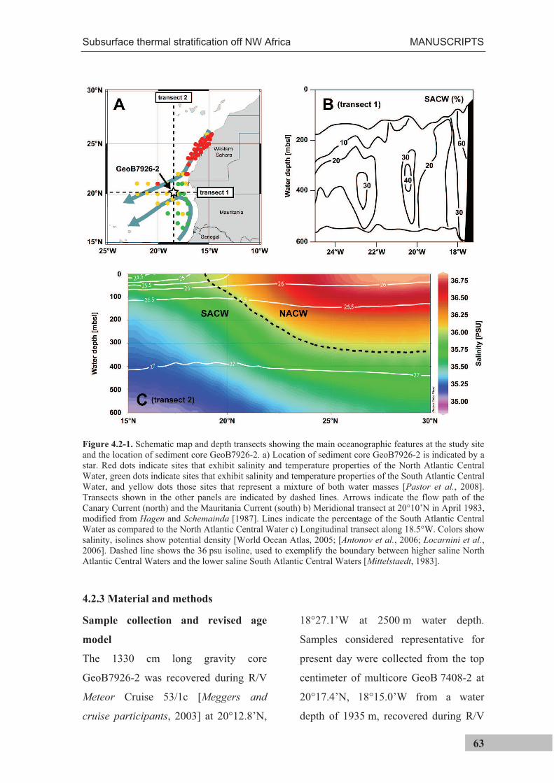
Subsurface thermal stratification off NW Africa MANUSCRIPTS
63
Figure 4.2-1. Schematic map and depth transects showing the main oceanographic features at the study site and the location of sediment core GeoB7926-2. a) Location of sediment core GeoB7926-2 is indicated by a star. Red dots indicate sites that exhibit salinity and temperature properties of the North Atlantic Central Water, green dots indicate sites that exhibit salinity and temperature properties of the South Atlantic Central Water, and yellow dots those sites that represent a mixture of both water masses [Pastor et al., 2008]. Transects shown in the other panels are indicated by dashed lines. Arrows indicate the flow path of the Canary Current (north) and the Mauritania Current (south) b) Meridional transect at 20°10’N in April 1983, modified from Hagen and Schemainda [1987]. Lines indicate the percentage of the South Atlantic Central Water as compared to the North Atlantic Central Water c) Longitudinal transect along 18.5°W. Colors show salinity, isolines show potential density [World Ocean Atlas, 2005; [Antonov et al., 2006; Locarnini et al.,2006]. Dashed line shows the 36 psu isoline, used to exemplify the boundary between higher saline North Atlantic Central Waters and the lower saline South Atlantic Central Waters [Mittelstaedt, 1983].
4.2.3 Material and methods
Sample collection and revised age
model
The 1330 cm long gravity core
GeoB7926-2 was recovered during R/V
Meteor Cruise 53/1c [Meggers and
cruise participants, 2003] at 20°12.8’N,
18°27.1’W at 2500 m water depth.
Samples considered representative for
present day were collected from the top
centimeter of multicore GeoB 7408-2 at
20°17.4’N, 18°15.0’W from a water
depth of 1935 m, recovered during R/V
MANUSCRIPTS Subsurface thermal stratification off NW Africa
64
Poseidon cruise 272 [Meggers et al.,
2002]. Sediment sample were wet-sieved
(>63um) and the residual dry-sieved into
two size fractions, 63-150 µm and
>150 µm. From the >150 µm size
fraction specimens of the planktic
foraminifer G. inflata were hand-picked
under a binocular microscope (largest
diameter 400-560 µm; most specimen
400-480 µm). Samples were weighted in
three replicates with a microbalance and
only specimens strictly between 20 and
50 µg are used in the discussion.
The age model of the upper 820 cm is
based on 12 Accelerator Mass
Spectrometry (AMS) 14C dates on
monospecific samples of the planktonic
foraminifera G. inflata and covers
approximately the last 24 kyrs.
Radiocarbon ages have been previously
published [Romero et al., 2008]. We
revised the age model, converting
radiocarbon ages into calendar years
using the Calib Rev 6.1.0 program, with
the most recent marine calibration
dataset marine09.14c [Reimer et al.,
2009]. We acknowledge that the dated
species G. inflata was possibly exposed
to water exceeding the global reservoir
age of ~400 yrs. We hence calculated the
calendar age that would be associated
with an additional local reservoir age of
197 yrs. This is the local reservoir age
further south, where old South Atlantic
Central Water is upwelled
(http://www.calib.qub.ac.uk/marine/regi
oncalc.php), likely exhibiting the oldest
reservoir age at the study site. In Table
4.2-1, we show calculated calendar ages
assuming no reservoir age and in Table
4.2-2 assuming a reservoir age of
197 yrs, to show the effect this has on
the calculated calendar ages.
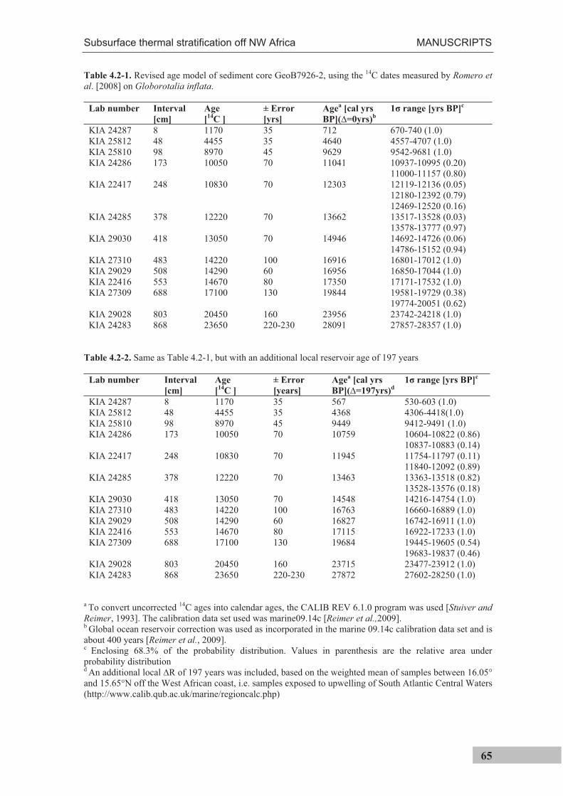
Subsurface thermal stratification off NW Africa MANUSCRIPTS
65
Table 4.2-1. Revised age model of sediment core GeoB7926-2, using the 14C dates measured by Romero et al. [2008] on Globorotalia inflata.
Lab number Interval
[cm]
Age
[14
C ]
± Error
[yrs]
Agea [cal yrs
BP]( =0yrs)b
1 range [yrs BP]c
KIA 24287 8 1170 35 712 670-740 (1.0) KIA 25812 48 4455 35 4640 4557-4707 (1.0) KIA 25810 98 8970 45 9629 9542-9681 (1.0) KIA 24286 173 10050 70 11041 10937-10995 (0.20)
11000-11157 (0.80) KIA 22417 248 10830 70 12303 12119-12136 (0.05)
12180-12392 (0.79) 12469-12520 (0.16)
KIA 24285 378 12220 70 13662 13517-13528 (0.03) 13578-13777 (0.97)
KIA 29030 418 13050 70 14946 14692-14726 (0.06) 14786-15152 (0.94)
KIA 27310 483 14220 100 16916 16801-17012 (1.0) KIA 29029 508 14290 60 16956 16850-17044 (1.0) KIA 22416 553 14670 80 17350 17171-17532 (1.0) KIA 27309 688 17100 130 19844 19581-19729 (0.38)
19774-20051 (0.62) KIA 29028 803 20450 160 23956 23742-24218 (1.0) KIA 24283 868 23650 220-230 28091 27857-28357 (1.0)
Table 4.2-2. Same as Table 4.2-1, but with an additional local reservoir age of 197 years
Lab number Interval
[cm]
Age
[14
C ]
± Error
[years]
Agea [cal yrs
BP]( =197yrs)d
1 range [yrs BP]c
KIA 24287 8 1170 35 567 530-603 (1.0) KIA 25812 48 4455 35 4368 4306-4418(1.0) KIA 25810 98 8970 45 9449 9412-9491 (1.0) KIA 24286 173 10050 70 10759 10604-10822 (0.86)
10837-10883 (0.14) KIA 22417 248 10830 70 11945 11754-11797 (0.11)
11840-12092 (0.89) KIA 24285 378 12220 70 13463 13363-13518 (0.82)
13528-13576 (0.18) KIA 29030 418 13050 70 14548 14216-14754 (1.0) KIA 27310 483 14220 100 16763 16660-16889 (1.0) KIA 29029 508 14290 60 16827 16742-16911 (1.0) KIA 22416 553 14670 80 17115 16922-17233 (1.0) KIA 27309 688 17100 130 19684 19445-19605 (0.54)
19683-19837 (0.46) KIA 29028 803 20450 160 23715 23477-23912 (1.0) KIA 24283 868 23650 220-230 27872 27602-28250 (1.0)
a To convert uncorrected 14C ages into calendar ages, the CALIB REV 6.1.0 program was used [Stuiver and Reimer, 1993]. The calibration data set used was marine09.14c [Reimer et al.,2009]. b Global ocean reservoir correction was used as incorporated in the marine 09.14c calibration data set and is about 400 years [Reimer et al., 2009]. c Enclosing 68.3% of the probability distribution. Values in parenthesis are the relative area under probability distribution d An additional local R of 197 years was included, based on the weighted mean of samples between 16.05° and 15.65°N off the West African coast, i.e. samples exposed to upwelling of South Atlantic Central Waters (http://www.calib.qub.ac.uk/marine/regioncalc.php)
MANUSCRIPTS Subsurface thermal stratification off NW Africa
66
Analytical approach
Mg/Ca thermometry
For Mg/Ca measurements, about 20
specimens of G. inflata were gently
crushed and cleaned following the
protocol described in Barker et al.
[2003]. Samples were washed seven
times with suprapure water, twice with
methanol followed by two oxidation
steps of 10 min and a weak acid leach in
0.001M TD HNO3. Samples were then
centrifuged for 10 min at 6000 rpm,
transferred into test tubes and diluted.
Mg/Ca ratios were measured on a
Perkin-Elmer Optima 3300R inductively
coupled plasma-optical emission
spectrometer (ICP-OES) equipped with
an ultrasonic nebulizer U-5000 AT
(Cetac Technologies Inc.) and on a
Agilent Technologies 700 Series ICP-
OES, at the faculty of Geosciences and
the Center for Marine Environmental
Sciences, University of Bremen. During
the analysis, the measured Mg/Ca ratio
of carbonate reference material ECRM
752-1 was on average 3.84 mmol/mol
(n = 12; = 0.04), in good agreement
with the reported Mg/Ca ratio of
3.75 mmol/mol [Greaves et al., 2008].
The precision of measurements on
G. inflata was on average
0.004 mmol/mol, based on mostly three
(n=111) and few times (n=17) two
replicates. Mg/Ca temperatures were
calculated using the equation of
Elderfield and Ganssen [2000] (equation
4.2-1).
T = LN ((Mg/Ca)/0.49)/0.1)
(4.2-1)
Single specimen oxygen isotope
analysis
Planktic foraminifera calcify over a
period of a couple of weeks to months
[Bé and Spero, 1981; Hemleben et al.,
1989]. This short calcification period
implies that their shell chemistry records
temperatures that prevailed during this
particular period. When a large amount
of individual shells from the sedimentary
record is analyzed, these were likely
formed during different periods. By
comparison of individual shells of
surface dwelling species, seasonal
temperature ranges may be assessed
[e.g.; Ganssen et al., 2010; Wit et al.,
2010; Haarmann et al., 2011].
In contrast shells of intermediate
depth-dwelling foraminifera calcify over
a large depth range [Wilke et al., 2006],
implying that the geochemical signal of
an individual shell reflects the
environmental conditions throughout this
depth range, centered at the depth were
the gross of the calcite was formed.
Subsurface thermal stratification off NW Africa MANUSCRIPTS
67
)13(*5.13),13(*5.11 QQQQQQ
Assuming that a population of
intermediate depth-dwelling foraminifera
did not change its habitat in the past,
individual shells have been used to
assess changes at these depths of main
calcification [Leduc et al., 2009; Khider
et al., 2011].
In this study, temperatures are
reconstructed from individual shells of
G. inflata, assuming that these reflect
temperatures over the depth range
inhabited by this species at present day.
To capture the spread in the calcification
temperatures of G. inflata, the stable
oxygen isotope composition of
individual shells was measured. We
reconstructed calcification temperature
ranges from between 21 and 43 single
specimens of G. inflata. After weighing
in three replicates on a microbalance,
oxygen isotopes were determined on a
Finnigan MAT 252 mass spectrometer
coupled to a Kiel preparation device,
housed at the Vrije Universiteit in
Amsterdam (VUA), The Netherlands.
Reproducibility of VUA standard
calibrated against National Bureau of
Standards NBS-20 carbonate standard
was 0.10 ‰ (1 ) over all analytical
sessions. In order to exclude potential
outliers, we do not interpret data which
fall outside the range
(4.2-2)
with Q1 and Q3 being the first and the
third quartile of the data, respectively.
Potential outliers, identified using this
method, are indicated in Table 4.2-S1.
In order to calculate temperatures from
oxygen isotopes of individual shells, the
previously established Mg/Ca
temperatures combined with the average 18Oc of the individual oxygen isotope
measurements at the respective core
depths were used in equation 4.2-3 in
order to calculate 18Oseawater. The
equation is reported solved for 18Oseawater and based on the equation of
Kim and O’Neil [1997] in its rewritten
form [Bemis et al., 1998].
(4.2-3)
Assuming that both, the Mg/Ca multi
specimen and the average 18Oc single
specimen values mirror the mean
calcification temperature, temperatures
of every single specimen oxygen isotope
measurement around the average Mg/Ca
temperature can be used to estimate
calcification temperature ranges,
applying the equation in its form solved
for temperature (equation 4.2-4).
09.0*2
1.16*09.0*464.464.4 2
1818
T
OO calciteseawater
MANUSCRIPTS Subsurface thermal stratification off NW Africa
68
(4.2-4)
We calculated expected equilibrium
values ( 18Oeq) for various water depths
and seasons using the rearranged
equation of Kim and O’Neil [1997]
(equation 4.2-5).
(4.2-5)
18Ow was estimated from salinity data
[World Ocean Atlas, 2005; Antonov et
al., 2006], used in equation 4.2-6.
Equation 4.2-6 is based on the local 18Ow:salinity relationship between 18.4°
and 20.5°N and 18.1° and 21.2°W,
calculated from Pierre et al. [1994], as
provided in the global seawater 18O
database [Schmidt, G.A., G. R. Bigg and
E. J. Rohling, 1999;
http://data.giss.nasa.gov/o18data/].
18Ow = 0.4664*salinity – 16.024
(4.2-6)
Statistics
In order to determine, if the standard
deviation of the single specimen oxygen
isotope measurements in the past
differed from the near present day
standard deviation, the confidence
interval of the 8 cm sediment depth
standard deviation was calculated
according to equation 4.2-7, where is
the standard deviation, n the number of
samples and =0.05 defines the 95%
confidence level.
(4.2-7)
Model
In this study, we present model results
from simulations using the
comprehensive Community Climate
System Model Version 3 (CCSM3; see
Collins et al., 2006 for an overview) in
its coarse-resolution setup [Yeager et al.,
2006] to simulate the climates of the Last
Glacial Maximum (LGM) and Heinrich
event/stadial 1 (HE1). Details on these
glacial simulations and on a preindustrial
control simulation used as a reference
can be found in Merkel et al. [2010]. In
the glacial simulations, changes of the
orbital parameters, greenhouse gas
concentrations, ice sheet albedo and
topography as well as the lowering of the
sea level during the LGM are taken into
account. In addition, for the Heinrich
simulation, a permanent freshwater
anomaly over the Greenland-Iceland-
Norwegian Seas is imposed to the glacial
ocean, thereby inducing a pronounced
21818
1818
)(*09.0
)(*64.41.16
seawatercalcite
seawatercalcite
OO
OOT
704.43*333.3778.251818 TOO Weq
)2
1,1(/)1(*,)2
,1(/)1(* 22 nnnn
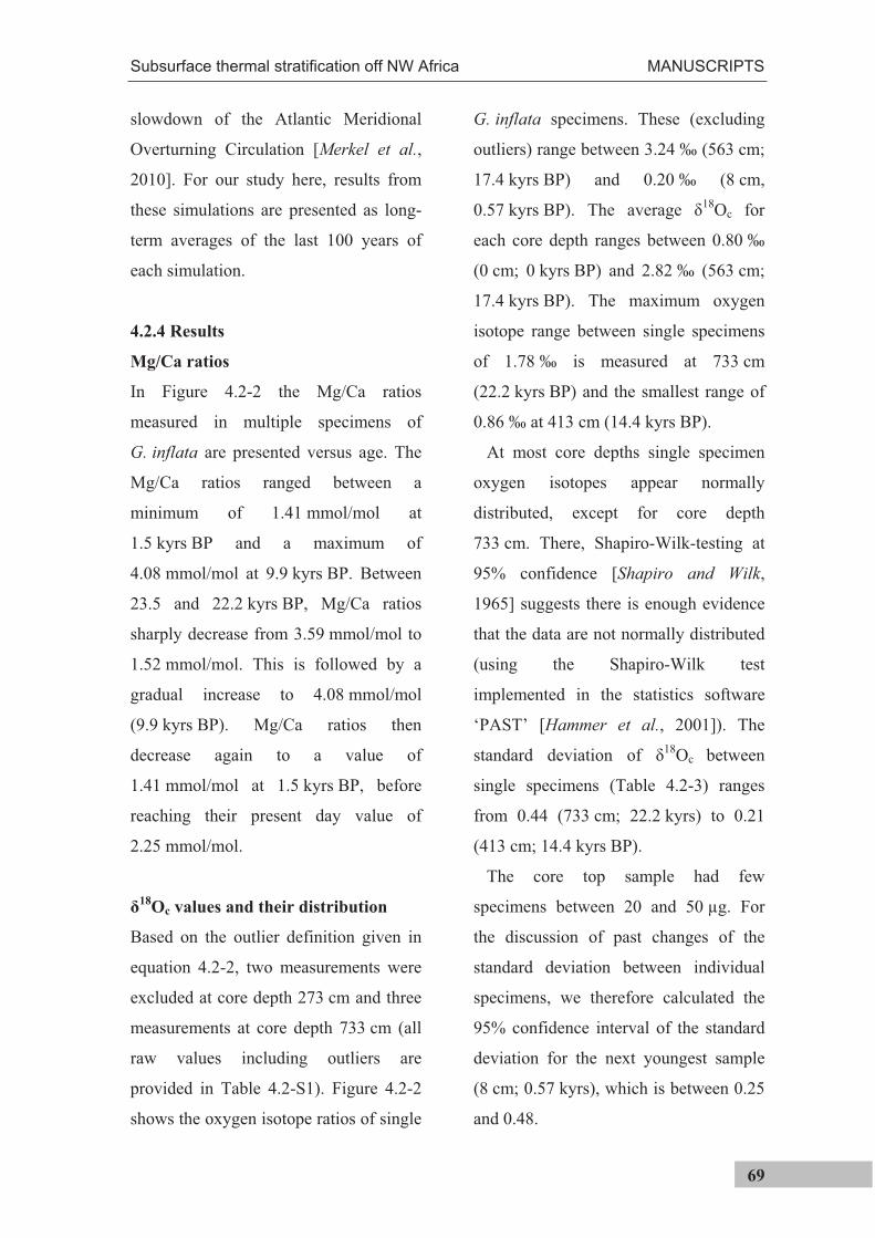
Subsurface thermal stratification off NW Africa MANUSCRIPTS
69
slowdown of the Atlantic Meridional
Overturning Circulation [Merkel et al.,
2010]. For our study here, results from
these simulations are presented as long-
term averages of the last 100 years of
each simulation.
4.2.4 Results
Mg/Ca ratios
In Figure 4.2-2 the Mg/Ca ratios
measured in multiple specimens of
G. inflata are presented versus age. The
Mg/Ca ratios ranged between a
minimum of 1.41 mmol/mol at
1.5 kyrs BP and a maximum of
4.08 mmol/mol at 9.9 kyrs BP. Between
23.5 and 22.2 kyrs BP, Mg/Ca ratios
sharply decrease from 3.59 mmol/mol to
1.52 mmol/mol. This is followed by a
gradual increase to 4.08 mmol/mol
(9.9 kyrs BP). Mg/Ca ratios then
decrease again to a value of
1.41 mmol/mol at 1.5 kyrs BP, before
reaching their present day value of
2.25 mmol/mol.
18Oc values and their distribution
Based on the outlier definition given in
equation 4.2-2, two measurements were
excluded at core depth 273 cm and three
measurements at core depth 733 cm (all
raw values including outliers are
provided in Table 4.2-S1). Figure 4.2-2
shows the oxygen isotope ratios of single
G. inflata specimens. These (excluding
outliers) range between 3.24 ‰ (563 cm;
17.4 kyrs BP) and 0.20 ‰ (8 cm,
0.57 kyrs BP). The average 18Oc for
each core depth ranges between 0.80 ‰
(0 cm; 0 kyrs BP) and 2.82 ‰ (563 cm;
17.4 kyrs BP). The maximum oxygen
isotope range between single specimens
of 1.78 ‰ is measured at 733 cm
(22.2 kyrs BP) and the smallest range of
0.86 ‰ at 413 cm (14.4 kyrs BP).
At most core depths single specimen
oxygen isotopes appear normally
distributed, except for core depth
733 cm. There, Shapiro-Wilk-testing at
95% confidence [Shapiro and Wilk,
1965] suggests there is enough evidence
that the data are not normally distributed
(using the Shapiro-Wilk test
implemented in the statistics software
‘PAST’ [Hammer et al., 2001]). The
standard deviation of 18
Oc between
single specimens (Table 4.2-3) ranges
from 0.44 (733 cm; 22.2 kyrs) to 0.21
(413 cm; 14.4 kyrs BP).
The core top sample had few
specimens between 20 and 50 µg. For
the discussion of past changes of the
standard deviation between individual
specimens, we therefore calculated the
95% confidence interval of the standard
deviation for the next youngest sample
(8 cm; 0.57 kyrs), which is between 0.25
and 0.48.
MANUSCRIPTS Subsurface thermal stratification off NW Africa
70
Table 4.2-3. Average 18Oc values [‰ vs. PDB], standard deviation (underlined when significantly
different from the most recent sample) and p value of Shapiro-Wilk test, derived from individual specimens
of G. inflata from sediment core GeoB7926-2 at selected core depths.
Age
(Depth)n
Average 18
Oc
[‰ vs. PDB]
p(normal) p(normal)>0.05
0.57 kyrs BP
(8 cm) 21 0.86 0.33 0.263 Yes
6.16 kyrs BP
(78 cm) 30 0.87 0.41 0.473 Yes
12.26kyrs BP
(273 cm)
231.76 0.22 0.061 Yes
14.41kyrs BP
(413 cm) 41 2.36 0.21 0.860 Yes
16.80 kyrs BP
(498 cm) 43 2.31 0.23 0.459 Yes
17.36 kyrs BP
(563 cm) 24 2.82 0.32 0.054 Yes
22.18 kyrs BP
(733 cm) 39 1.90 0.44 0.026 No
Subsurface thermal stratification off NW Africa MANUSCRIPTS
71
Figure 4.2-2 (previous page). Results of the single specimen 18Oc and multi-specimen Mg/Ca
measurements in sediment core GeoB7926-2. a) Oxygen isotopes of G. bulloides (line) in sediment core
GeoB7926-2 [Romero et al., 2008] and single G. inflata oxygen isotopes (circles). Youngest sample is from
the top centimeter of multicorer GeoB7408-2 [Meggers et al., 2002]. Red circles show measurements that
are considered outliers using the definition given in equation 4.2-2. Curve shows 18Oc of Cibicidoides wuellerstorfi [data: B. Donner]. b) Mg/Ca of multi-specimen measurements on G. inflata. Triangles on the
abscissa show 14C age control points revised from Romero et al. [2008]. LGM: Last Glacial Maximum,
HS1: Heinrich Stadial 1, B/A: Bølling-Allerød, YD: Younger Dryas.
4.2.5 Discussion
Single specimen temperatures reflect
thermal water column stratification
Modern observations show that Mg/Ca
ratios in single specimen of G. inflata at
the study site correspond to calcification
depths between the sea surface and
~400 m [Haarmann et al., 2011]. The
calcification depth derived from
analyzing multiple shells is about 150 m.
This means that the analysis of multiple
shells will to a limited extend only detect
a subsurface warming and stratification
changes that occur mostly below 100 m.
It is suggested that the analysis of
single specimens provides a more
detailed picture. In the case of a potential
subsurface warming off NW Africa
below 100 m, in particular the deepest
(i.e. indicative for the coldest
temperatures) individuals are expected to
be mostly affected by this warming.
Increased water column stratification is
expected to result in a decreased 18
Oc
standard deviation of the sampled
population, as a result of a narrowed
depth habitat.
Single specimen analysis requires that
the sampled population captures the full
calcification range, as observed in the
water column. Also, the single specimen
18Oc ranges must be independent of the
number of shells which are analyzed
(here r2 < 0.00) and
18Oc must be
independent of shell weights (here r2
between 0.00 and 0.39, see Figure 4.2-
S1). Finally, the calcification range of
the used size fraction must be well
known. For this, we confined our
analysis to the same size fraction (400-
560 µm; most specimen 400-480 µm)
and weights as in Haarmann et al.
[2011].
In Figure 4.2-3 and Table 4.2-4, we
present calculated seasonal oxygen
isotope equilibrium values (18
Oeq) for
February (most positive values) and
September (most negative values) in
order to assess the seasonal 18
Oeq range.
The calculation is based on monthly
temperature [Locarnini et al., 2006] and
salinity [Antonov et al., 2006], used in
equations 4.2-5 and 4.2-6, respectively.
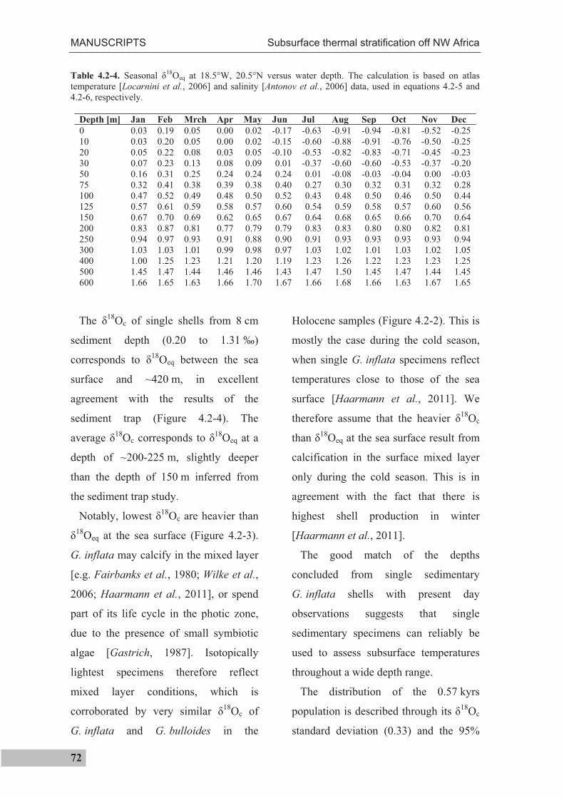
MANUSCRIPTS Subsurface thermal stratification off NW Africa
72
Table 4.2-4. Seasonal 18Oeq at 18.5°W, 20.5°N versus water depth. The calculation is based on atlas
temperature [Locarnini et al., 2006] and salinity [Antonov et al., 2006] data, used in equations 4.2-5 and
4.2-6, respectively.
Depth [m] Jan Feb Mrch Apr May Jun Jul Aug Sep Oct Nov Dec
0 0.03 0.19 0.05 0.00 0.02 -0.17 -0.63 -0.91 -0.94 -0.81 -0.52 -0.25
10 0.03 0.20 0.05 0.00 0.02 -0.15 -0.60 -0.88 -0.91 -0.76 -0.50 -0.25
20 0.05 0.22 0.08 0.03 0.05 -0.10 -0.53 -0.82 -0.83 -0.71 -0.45 -0.23
30 0.07 0.23 0.13 0.08 0.09 0.01 -0.37 -0.60 -0.60 -0.53 -0.37 -0.20
50 0.16 0.31 0.25 0.24 0.24 0.24 0.01 -0.08 -0.03 -0.04 0.00 -0.03
75 0.32 0.41 0.38 0.39 0.38 0.40 0.27 0.30 0.32 0.31 0.32 0.28
100 0.47 0.52 0.49 0.48 0.50 0.52 0.43 0.48 0.50 0.46 0.50 0.44
125 0.57 0.61 0.59 0.58 0.57 0.60 0.54 0.59 0.58 0.57 0.60 0.56
150 0.67 0.70 0.69 0.62 0.65 0.67 0.64 0.68 0.65 0.66 0.70 0.64
200 0.83 0.87 0.81 0.77 0.79 0.79 0.83 0.83 0.80 0.80 0.82 0.81
250 0.94 0.97 0.93 0.91 0.88 0.90 0.91 0.93 0.93 0.93 0.93 0.94
300 1.03 1.03 1.01 0.99 0.98 0.97 1.03 1.02 1.01 1.03 1.02 1.05
400 1.00 1.25 1.23 1.21 1.20 1.19 1.23 1.26 1.22 1.23 1.23 1.25
500 1.45 1.47 1.44 1.46 1.46 1.43 1.47 1.50 1.45 1.47 1.44 1.45
600 1.66 1.65 1.63 1.66 1.70 1.67 1.66 1.68 1.66 1.63 1.67 1.65
The18
Oc of single shells from 8 cm
sediment depth (0.20 to 1.31 ‰)
corresponds to 18
Oeq between the sea
surface and ~420 m, in excellent
agreement with the results of the
sediment trap (Figure 4.2-4). The
average18
Oc corresponds to 18
Oeq at a
depth of ~200-225 m, slightly deeper
than the depth of 150 m inferred from
the sediment trap study.
Notably, lowest 18
Oc are heavier than
18Oeq at the sea surface (Figure 4.2-3).
G. inflata may calcify in the mixed layer
[e.g. Fairbanks et al., 1980; Wilke et al.,
2006; Haarmann et al., 2011], or spend
part of its life cycle in the photic zone,
due to the presence of small symbiotic
algae [Gastrich, 1987]. Isotopically
lightest specimens therefore reflect
mixed layer conditions, which is
corroborated by very similar 18
Oc of
G. inflata and G. bulloides in the
Holocene samples (Figure 4.2-2). This is
mostly the case during the cold season,
when single G. inflata specimens reflect
temperatures close to those of the sea
surface [Haarmann et al., 2011]. We
therefore assume that the heavier 18
Oc
than18
Oeq at the sea surface result from
calcification in the surface mixed layer
only during the cold season. This is in
agreement with the fact that there is
highest shell production in winter
[Haarmann et al., 2011].
The good match of the depths
concluded from single sedimentary
G. inflata shells with present day
observations suggests that single
sedimentary specimens can reliably be
used to assess subsurface temperatures
throughout a wide depth range.
The distribution of the 0.57 kyrs
population is described through its 18
Oc
standard deviation (0.33) and the 95%
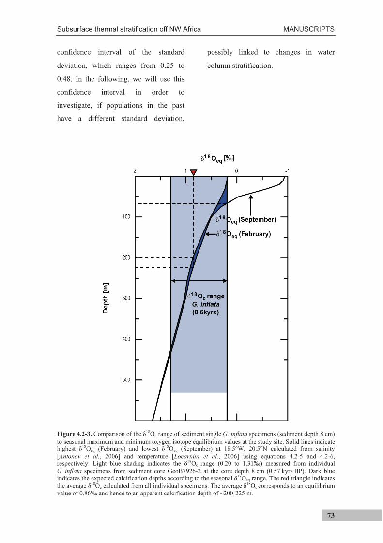
Subsurface thermal stratification off NW Africa MANUSCRIPTS
73
confidence interval of the standard
deviation, which ranges from 0.25 to
0.48. In the following, we will use this
confidence interval in order to
investigate, if populations in the past
have a different standard deviation,
possibly linked to changes in water
column stratification.
Figure 4.2-3. Comparison of the 18Oc range of sediment single G. inflata specimens (sediment depth 8 cm)
to seasonal maximum and minimum oxygen isotope equilibrium values at the study site. Solid lines indicate
highest 18Oeq (February) and lowest 18Oeq (September) at 18.5°W, 20.5°N calculated from salinity
[Antonov et al., 2006] and temperature [Locarnini et al., 2006] using equations 4.2-5 and 4.2-6,
respectively. Light blue shading indicates the 18Oc range (0.20 to 1.31‰) measured from individual
G. inflata specimens from sediment core GeoB7926-2 at the core depth 8 cm (0.57 kyrs BP). Dark blue
indicates the expected calcification depths according to the seasonal 18Oeq range. The red triangle indicates
the average 18Oc calculated from all individual specimens. The average 18Oc corresponds to an equilibrium
value of 0.86‰ and hence to an apparent calcification depth of ~200-225 m.
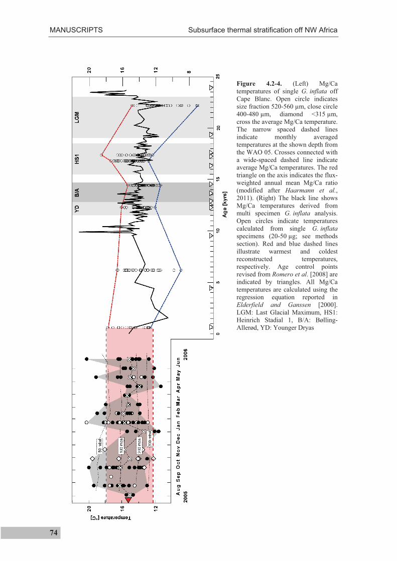
MANUSCRIPTS Subsurface thermal stratification off NW Africa
74
Figure 4.2-4. (Left) Mg/Ca
temperatures of single G. inflata off
Cape Blanc. Open circle indicates
size fraction 520-560 µm, close circle
400-480 µm, diamond <315 µm, cross the average Mg/Ca temperature. The narrow spaced dashed lines indicate monthly averaged temperatures at the shown depth from the WAO 05. Crosses connected with a wide-spaced dashed line indicate average Mg/Ca temperatures. The red triangle on the axis indicates the flux-weighted annual mean Mg/Ca ratio (modified after Haarmann et al.,2011). (Right) The black line shows Mg/Ca temperatures derived from multi specimen G. inflata analysis. Open circles indicate temperatures calculated from single G. inflataspecimens (20-50 µg; see methods section). Red and blue dashed lines illustrate warmest and coldest reconstructed temperatures, respectively. Age control points revised from Romero et al. [2008] are indicated by triangles. All Mg/Ca temperatures are calculated using the regression equation reported in Elderfield and Ganssen [2000]. LGM: Last Glacial Maximum, HS1: Heinrich Stadial 1, B/A: Bølling-Allerød, YD: Younger Dryas

Subsurface thermal stratification off NW Africa MANUSCRIPTS
75
Paleoceanographic applicability of
single G. inflata specimens
We have demonstrated earlier that the
18Oc range of single G. inflata shells
matches the present day calcification
temperature range of the upper water
column from near surface values down
to about 425 m. It can be expected that a
subsurface warming below ~100 m will
preferentially raise the lowest
calcification temperature.
Furthermore, considering all single
specimens of a sampled population, this
must consequently result in a reduced
18Oc standard deviation. As can be seen
in Figure 4.2-5, this indeed is the fact for
the deglacial samples between 16.8 and
12.3 kyrs BP all having a standard
deviation outside of the 95% confidence
interval of the standard deviation of the
0.57 kyrs BP sample (Table 4.2-3).
It is interesting to note that changes of
the temperature range between intervals
with a large and a small range (i.e. 22.2
to 17.4 kyrs BP and 12.3 to 6.2 kyrs BP;
Figure 4.2-5) are largely due to a
different number of specimens
representing the temperature minima.
We interpret this as a result of a
subsurface warming and/or changes of
water column stratification taking place
at the lower habitat depth of G. inflata.
This observation also suggests that a
warming is unlikely to have a surface
Figure 4.2-5. Distribution of temperatures
calculated from the oxygen isotopic composition
of single specimens of G. inflata in sediment
core GeoB7926-2. Calculation of temperatures is
explained in the main text. Red histograms have
a different 18Oc standard deviation from the
0.57 kyrs sample; blue histograms have a
statistically identical standard deviation.
Temperatures that do not deviate enough from a
normal distribution to conclude that they are non-
normally distributed (Shapiro-Wilk tested at the
95% confidence level) are shown with a
Gaussian fit. Arrows with numbers show
temperature difference to the next younger
sample.
origin and/or results from a stronger
mixing of the water column, since this
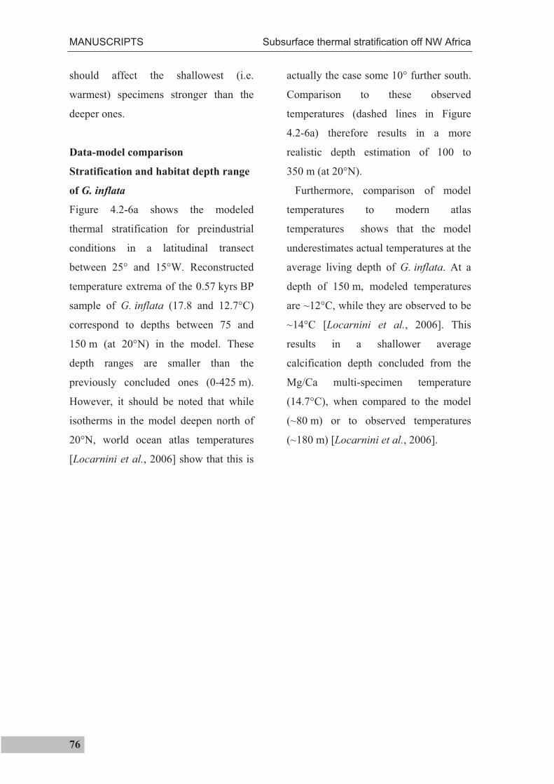
MANUSCRIPTS Subsurface thermal stratification off NW Africa
76
should affect the shallowest (i.e.
warmest) specimens stronger than the
deeper ones.
Data-model comparison
Stratification and habitat depth range
of G. inflata
Figure 4.2-6a shows the modeled
thermal stratification for preindustrial
conditions in a latitudinal transect
between 25° and 15°W. Reconstructed
temperature extrema of the 0.57 kyrs BP
sample of G. inflata (17.8 and 12.7°C)
correspond to depths between 75 and
150 m (at 20°N) in the model. These
depth ranges are smaller than the
previously concluded ones (0-425 m).
However, it should be noted that while
isotherms in the model deepen north of
20°N, world ocean atlas temperatures
[Locarnini et al., 2006] show that this is
actually the case some 10° further south.
Comparison to these observed
temperatures (dashed lines in Figure
4.2-6a) therefore results in a more
realistic depth estimation of 100 to
350 m (at 20°N).
Furthermore, comparison of model
temperatures to modern atlas
temperatures shows that the model
underestimates actual temperatures at the
average living depth of G. inflata. At a
depth of 150 m, modeled temperatures
are ~12°C, while they are observed to be
~14°C [Locarnini et al., 2006]. This
results in a shallower average
calcification depth concluded from the
Mg/Ca multi-specimen temperature
(14.7°C), when compared to the model
(~80 m) or to observed temperatures
(~180 m) [Locarnini et al., 2006].
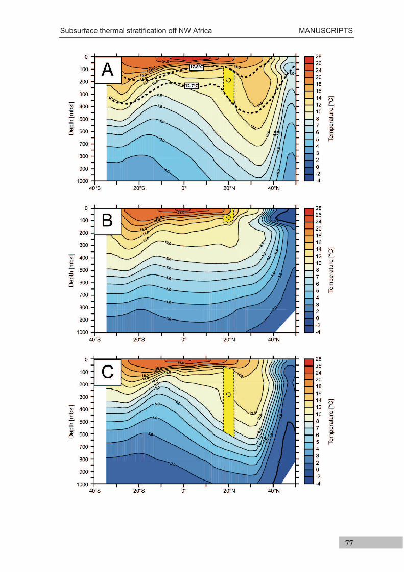
Subsurface thermal stratification off NW Africa MANUSCRIPTS
77
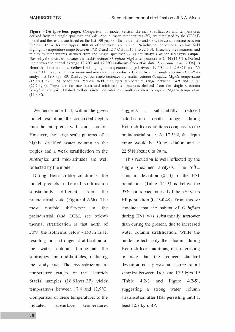
MANUSCRIPTS Subsurface thermal stratification off NW Africa
78
Figure 4.2-6 (previous page). Comparison of model vertical thermal stratification and temperatures
derived from the single specimen analysis. Annual mean temperatures (°C) are simulated by the CCSM3
model and the results are based on the last 100 years of the model runs and show the zonal average between
25° and 15°W for the upper 1000 m of the water column. a) Preindustrial conditions. Yellow field
highlights temperature range between 17.8°C and 12.7°C from 17.5 to 22.5°N. These are the maximum and
minimum temperatures derived from the single specimen G. inflata analysis of the 0.57 kyrs sample.
Dashed yellow circle indicates the multispecimen G. inflata Mg/Ca temperature at 20°N (14.7°C). Dashed
line shows the annual average 12.7°C and 17.8°C isotherms from atlas data [Locarnini et al., 2006] b)
Heinrich-like conditions. Yellow field highlights temperature range between 17.4°C and 12.9°C from 17.5
to 22.5°N. These are the maximum and minimum temperatures derived from the single specimen G. inflata analysis at 16.8 kyrs BP. Dashed yellow circle indicates the multispecimen G. inflata Mg/Ca temperature
(15.1°C) c) LGM conditions. Yellow field highlights temperature range between 14.9 and 7.0°C
(22.2 kyrs). These are the maximum and minimum temperatures derived from the single specimen
G. inflata analysis. Dashed yellow circle indicates the multispecimen G. inflata Mg/Ca temperature
(11.3°C).
We hence note that, within the given
model resolution, the concluded depths
must be interpreted with some caution.
However, the large scale patterns of a
highly stratified water column in the
tropics and a weak stratification in the
subtropics and mid-latitudes are well
reflected by the model.
During Heinrich-like conditions, the
model predicts a thermal stratification
substantially different from the
preindustrial state (Figure 4.2-6b). The
most notable difference to the
preindustrial (and LGM, see below)
thermal stratification is that north of
20°N the isotherms below ~150 m raise,
resulting in a stronger stratification of
the water column throughout the
subtropics and mid-latitudes, including
the study site. The reconstruction of
temperature ranges of the Heinrich
Stadial samples (16.8 kyrs BP) yields
temperatures between 17.4 and 12.9°C.
Comparison of these temperatures to the
modeled subsurface temperatures
suggests a substantially reduced
calcification depth range during
Heinrich-like conditions compared to the
preindustrial state. At 17.5°N, the depth
range would be 50 to ~100 m and at
22.5°N about 0 to 90 m.
This reduction is well reflected by the
single specimen analysis. The 18
Oc
standard deviation (0.23) of the HS1
population (Table 4.2-3) is below the
95% confidence interval of the 570 years
BP population (0.25-0.48). From this we
conclude that the habitat of G. inflata
during HS1 was substantially narrower
than during the present, due to increased
water column stratification. While the
model reflects only the situation during
Heinrich-like conditions, it is interesting
to note that the reduced standard
deviation is a persistent feature of all
samples between 16.8 and 12.3 kyrs BP
(Table 4.2-3 and Figure 4.2-5),
suggesting a strong water column
stratification after HS1 persisting until at
least 12.3 kyrs BP.
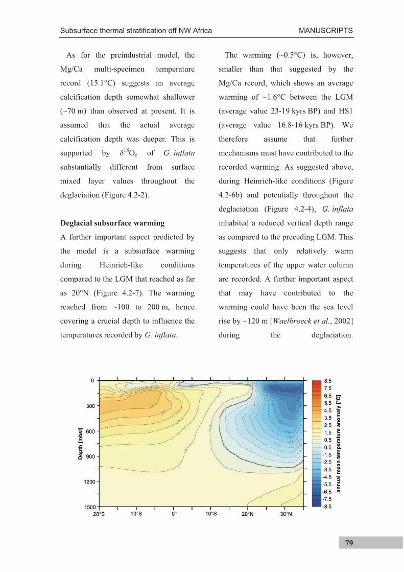
Subsurface thermal stratification off NW Africa MANUSCRIPTS
79
As for the preindustrial model, the
Mg/Ca multi-specimen temperature
record (15.1°C) suggests an average
calcification depth somewhat shallower
(~70 m) than observed at present. It is
assumed that the actual average
calcification depth was deeper. This is
supported by 18
Oc of G. inflata
substantially different from surface
mixed layer values throughout the
deglaciation (Figure 4.2-2).
Deglacial subsurface warming
A further important aspect predicted by
the model is a subsurface warming
during Heinrich-like conditions
compared to the LGM that reached as far
as 20°N (Figure 4.2-7). The warming
reached from ~100 to 200 m, hence
covering a crucial depth to influence the
temperatures recorded by G. inflata.
The warming (~0.5°C) is, however,
smaller than that suggested by the
Mg/Ca record, which shows an average
warming of ~1.6°C between the LGM
(average value 23-19 kyrs BP) and HS1
(average value 16.8-16 kyrs BP). We
therefore assume that further
mechanisms must have contributed to the
recorded warming. As suggested above,
during Heinrich-like conditions (Figure
4.2-6b) and potentially throughout the
deglaciation (Figure 4.2-4), G. inflata
inhabited a reduced vertical depth range
as compared to the preceding LGM. This
suggests that only relatively warm
temperatures of the upper water column
are recorded. A further important aspect
that may have contributed to the
warming could have been the sea level
rise by ~120 m [Waelbroeck et al., 2002]
during the deglaciation.
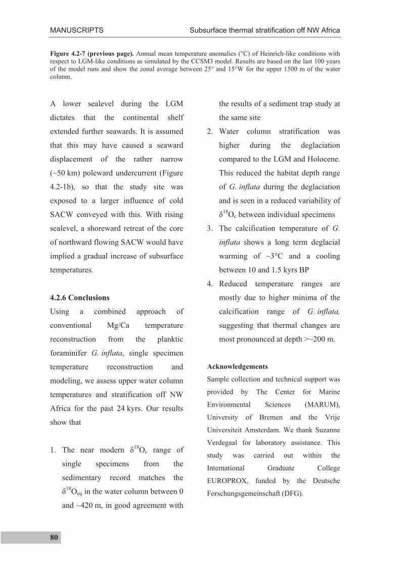
MANUSCRIPTS Subsurface thermal stratification off NW Africa
80
Figure 4.2-7 (previous page). Annual mean temperature anomalies (°C) of Heinrich-like conditions with
respect to LGM-like conditions as simulated by the CCSM3 model. Results are based on the last 100 years
of the model runs and show the zonal average between 25° and 15°W for the upper 1500 m of the water
column.
A lower sealevel during the LGM
dictates that the continental shelf
extended further seawards. It is assumed
that this may have caused a seaward
displacement of the rather narrow
(~50 km) poleward undercurrent (Figure
4.2-1b), so that the study site was
exposed to a larger influence of cold
SACW conveyed with this. With rising
sealevel, a shoreward retreat of the core
of northward flowing SACW would have
implied a gradual increase of subsurface
temperatures.
4.2.6 Conclusions
Using a combined approach of
conventional Mg/Ca temperature
reconstruction from the planktic
foraminifer G. inflata, single specimen
temperature reconstruction and
modeling, we assess upper water column
temperatures and stratification off NW
Africa for the past 24 kyrs. Our results
show that
1. The near modern 18
Oc range of
single specimens from the
sedimentary record matches the
18Oeq in the water column between 0
and ~420 m, in good agreement with
the results of a sediment trap study at
the same site
2. Water column stratification was
higher during the deglaciation
compared to the LGM and Holocene.
This reduced the habitat depth range
of G. inflata during the deglaciation
and is seen in a reduced variability of
18Oc between individual specimens
3. The calcification temperature of G.
inflata shows a long term deglacial
warming of ~3°C and a cooling
between 10 and 1.5 kyrs BP
4. Reduced temperature ranges are
mostly due to higher minima of the
calcification range of G. inflata,
suggesting that thermal changes are
most pronounced at depth >~200 m.
Acknowledgements
Sample collection and technical support was
provided by The Center for Marine
Environmental Sciences (MARUM),
University of Bremen and the Vrije
Universiteit Amsterdam. We thank Suzanne
Verdegaal for laboratory assistance. This
study was carried out within the
International Graduate College
EUROPROX, funded by the Deutsche
Forschungsgemeinschaft (DFG).
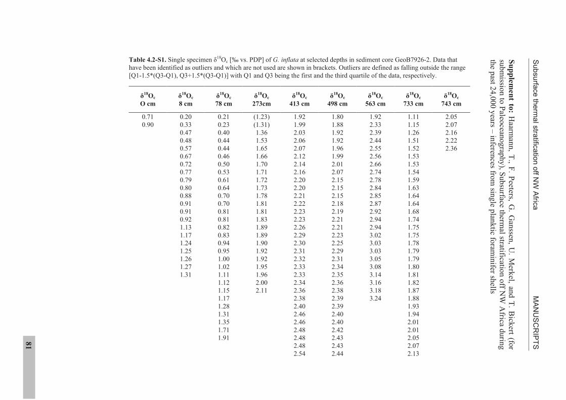
Su
bsu
rface
the
rma
l stra
tifica
tion
off N
W A
frica
MA
NU
SC
RIP
TS
81
Su
pp
lemen
t to:
Haarm
ann, T
., F. P
eeters, G. G
anssen
, U. M
erkel, an
d T
. Bick
ert (for
sub
missio
n to
Paleo
ceano
grap
hy
), Su
bsu
rface therm
al stratification
off N
W A
frica du
ring
the p
ast 24
,00
0 y
ears – in
ferences fro
m sin
gle p
lank
tic foram
inifer sh
ells
18Oc
743 cm
2.05
2.07
2.16
2.22
2.36
18Oc
733 cm
1.11
1.15
1.26
1.51
1.52
1.53
1.53
1.54
1.59
1.63
1.64
1.64
1.68
1.74
1.75
1.75
1.78
1.79
1.79
1.80
1.81
1.82
1.87
1.88
1.93
1.94
2.01
2.01
2.05
2.07
2.13
18Oc
563 cm
1.92
2.33
2.39
2.44
2.55
2.56
2.66
2.74
2.78
2.84
2.85
2.87
2.92
2.94
2.94
3.02
3.03
3.03
3.05
3.08
3.14
3.16
3.18
3.24
18Oc
498 cm
1.80
1.88
1.92
1.92
1.96
1.99
2.01
2.07
2.15
2.15
2.15
2.18
2.19
2.21
2.21
2.23
2.25
2.29
2.31
2.34
2.35
2.36
2.38
2.39
2.39
2.40
2.40
2.42
2.43
2.43
2.44
18Oc
413 cm
1.92
1.99
2.03
2.06
2.07
2.12
2.14
2.16
2.20
2.20
2.21
2.22
2.23
2.23
2.26
2.29
2.30
2.31
2.32
2.33
2.33
2.34
2.36
2.38
2.40
2.46
2.46
2.48
2.48
2.48
2.54
18Oc
273cm
(1.23)
(1.31)
1.36
1.53
1.65
1.66
1.70
1.71
1.72
1.73
1.78
1.81
1.81
1.83
1.89
1.89
1.90
1.92
1.92
1.95
1.96
2.00
2.11
18Oc
78 cm
0.21
0.23
0.40
0.44
0.44
0.46
0.50
0.53
0.61
0.64
0.70
0.70
0.81
0.81
0.82
0.83
0.94
0.95
1.00
1.02
1.11
1.12
1.15
1.17
1.28
1.31
1.35
1.71
1.91
18Oc
8 cm
0.20
0.33
0.47
0.48
0.57
0.67
0.72
0.77
0.79
0.80
0.88
0.91
0.91
0.92
1.13
1.17
1.24
1.25
1.26
1.27
1.31
Table 4.2-S1. Single specimen 18Oc [‰ vs. PDP] of G. inflata at selected depths in sediment core GeoB7926-2. Data that
have been identified as outliers and which are not used are shown in brackets. Outliers are defined as falling outside the range
[Q1-1.5*(Q3-Q1), Q3+1.5*(Q3-Q1)] with Q1 and Q3 being the first and the third quartile of the data, respectively.
18Oc
O cm
0.71
0.90
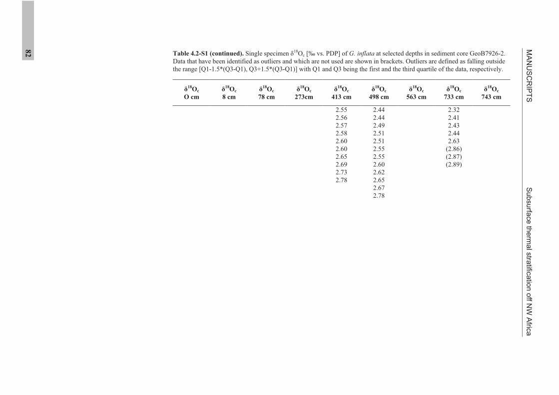
MA
NU
SC
RIP
TS
Su
bsu
rface
the
rma
l stra
tifica
tion
off N
W A
frica
82
18Oc
743 cm
18Oc
733 cm
2.32
2.41
2.43
2.44
2.63
(2.86)
(2.87)
(2.89)
18Oc
563 cm
18Oc
498 cm
2.44
2.44
2.49
2.51
2.51
2.55
2.55
2.60
2.62
2.65
2.67
2.78
18Oc
413 cm
2.55
2.56
2.57
2.58
2.60
2.60
2.65
2.69
2.73
2.78
18Oc
273cm
18Oc
78 cm
18Oc
8 cm
Table 4.2-S1 (continued). Single specimen 18Oc [‰ vs. PDP] of G. inflata at selected depths in sediment core GeoB7926-2.
Data that have been identified as outliers and which are not used are shown in brackets. Outliers are defined as falling outside
the range [Q1-1.5*(Q3-Q1), Q3+1.5*(Q3-Q1)] with Q1 and Q3 being the first and the third quartile of the data, respectively.
18Oc
O cm
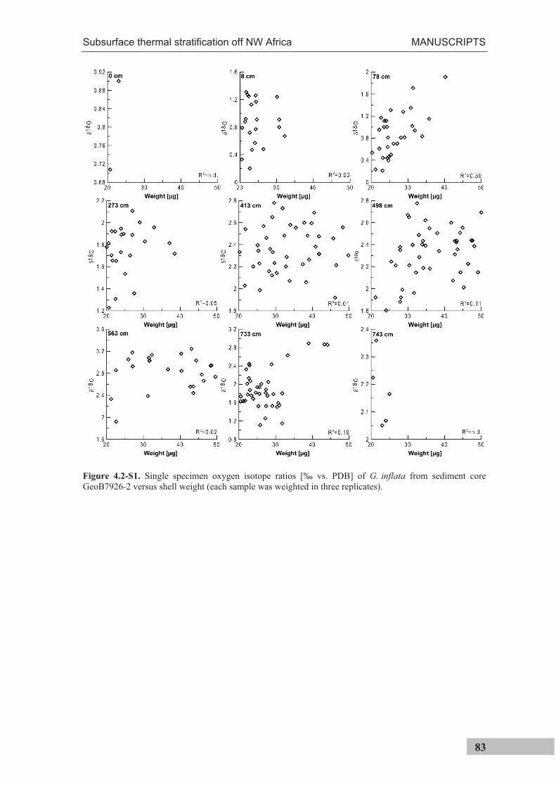
Subsurface thermal stratification off NW Africa MANUSCRIPTS
83
Figure 4.2-S1. Single specimen oxygen isotope ratios [‰ vs. PDB] of G. inflata from sediment core
GeoB7926-2 versus shell weight (each sample was weighted in three replicates).

84
Past upwelling strength off Cape Blanc MANUSCRIPTS
85
4.3 Manuscript 3
Upwelling strength off Cape Blanc (NW Africa) during the past 24,000 years –
Effects on the surface and subsurface Mg/Ca temperature records
Tim Haarmann, Mahyar Mohtadi, Jeroen Groeneveld, Torsten Bickert
Marum – Center for Marine Environmental Sciences, Leobener Straße, 28359 Bremen, Germany
In preparation for Biogeosciences
Upwelling of cold, nutrient rich subsurface waters is an important process that strongly
fosters productivity in the coastal area off NW Africa. Previous studies suggest increased
paleoproductivity along most of the NW African continental margin during the Last Glacial
Maximum (LGM), whereas off Cape Blanc (~20°N) decreased productivity was found. This
finding has been associated with a decrease of upwelling strength that has also been invoked
to explain unexpectedly warm local surface water temperatures during this cold climatic
state.
In the present study, we reconstruct upwelling strength off NW Africa for the past 24,000
years from the relative abundance of the planktic foraminifer Globigerina bulloides. Sea
surface temperatures (SST) were reconstructed using the Mg/Ca temperature proxy in the
surface-dwelling foraminifer species G. bulloides and Globigerinoides ruber (pink) and
compared to Mg/Ca temperatures of the subsurface-dwelling species Globorotalia inflata.
Despite of previous findings, G. bulloides abundances suggest a strong upwelling during
the LGM between 24 and 16 kyrs BP followed by a strong decrease afterwards. The
decrease in upwelling intensity coincides with a decrease of wind strength reconstructed in
other studies off Cape Blanc, suggesting a strong influence of wind strength on upwelling at
the study site. Reconstructed Mg/Ca temperature variability is generally high in the surface
dwelling species throughout the record. As no such variability is recorded in the
intermediate depth dwelling species G. inflata, the large temperature differences appear to
result from exceptionally large SST variability at the study site. Inspection of daily SSTs
between 1982 and 2008 from upwelling and non-upwelling months suggests that increased
wind strength has the potential to substantially increase local SSTs, likely through a
northward advection of warm southerly surface waters towards the study site. It is
presumed that also in the past this mechanism might have caused higher SSTs at the study
site during generally cold climatic states
MANUSCRIPTS Past upwelling strength off Cape Blanc
86
4.3.1 Introduction
The coastal area off NW Africa is one of
the four large global eastern boundary
upwelling systems of the subtropics.
Located at the eastern boundary of the
North Atlantic Subtropical Gyre, cold
and nutrient-rich subsurface waters are
pumped to the surface through Ekman-
transport from water depths between 100
and 300 m [Mittelstaedt, 1983]. This
important process enriches surface
waters with nutrients and strongly fosters
productivity [Fischer et al., 1996;
Helmke et al., 2005], which in turn
largely contributes to global primary
productivity and the sequestration of
carbon.
Considerable interest in the role of this
system related to climate change and
potential increase of upwelling strength
during the 20th
century [Bakun, 1990]
resulted in a multitude of reconstructions
of upwelling and productivity for the
past [e.g.; Chapman et al., 1996;
Martinez et al., 1999; Zhao et al., 2000;
Freudenthal et al., 2002; Kuhlmann et
al., 2004; Adkins et al., 2006; Haslett
and Smart, 2006; Romero et al., 2008;
Filipsson et al., 2011]. It is now clear
that this system is spatially very
heterogeneous. In particular off Cape
locations, where offshore advected
filaments develop [Pelegrí et al., 2005],
large uncertainties remain. A good
example for this phenomenon is the
perennial upwelling off Cape Blanc
(~21°N). While highest productivity is
reported for most of the NW African
continental margin during glacials [e.g.;
Abrantes, 2000; Freudenthal et al.,
2002; Henderiks et al., 2002] or the last
deglaciation [Kuhlmann et al., 2004],
reconstructions off Cape Blanc are
contradictory.
While decreased productivity is
attributed to more easterly winds,
effectively suppressing Ekman-induced
upwelling [Zhao et al., 2000], higher
productivity is attributed to stronger
northeast trade winds that modified the
direction an extent of the upwelling cell
[Chapman et al., 1996]. Since upwelling
can lower the sea surface temperature
(SST) by up to 6°C, a past decrease of
upwelling strength was invoked as a
possible mechanisms for explaining
unexpectedly warm SST off Cape Blanc
during the Last Glacial Maximum
(LGM) that exceeds those of the
preceding older glacial and the following
deglaciation [Zhao et al., 2000; Sicre et
al., 2001; Romero et al., 2008].
In the present study, we reconstruct the
upwelling strength off Cape Blanc for
the past 24,000 years based on the
relative abundance of the planktic
foraminifera Globigerina bulloides for
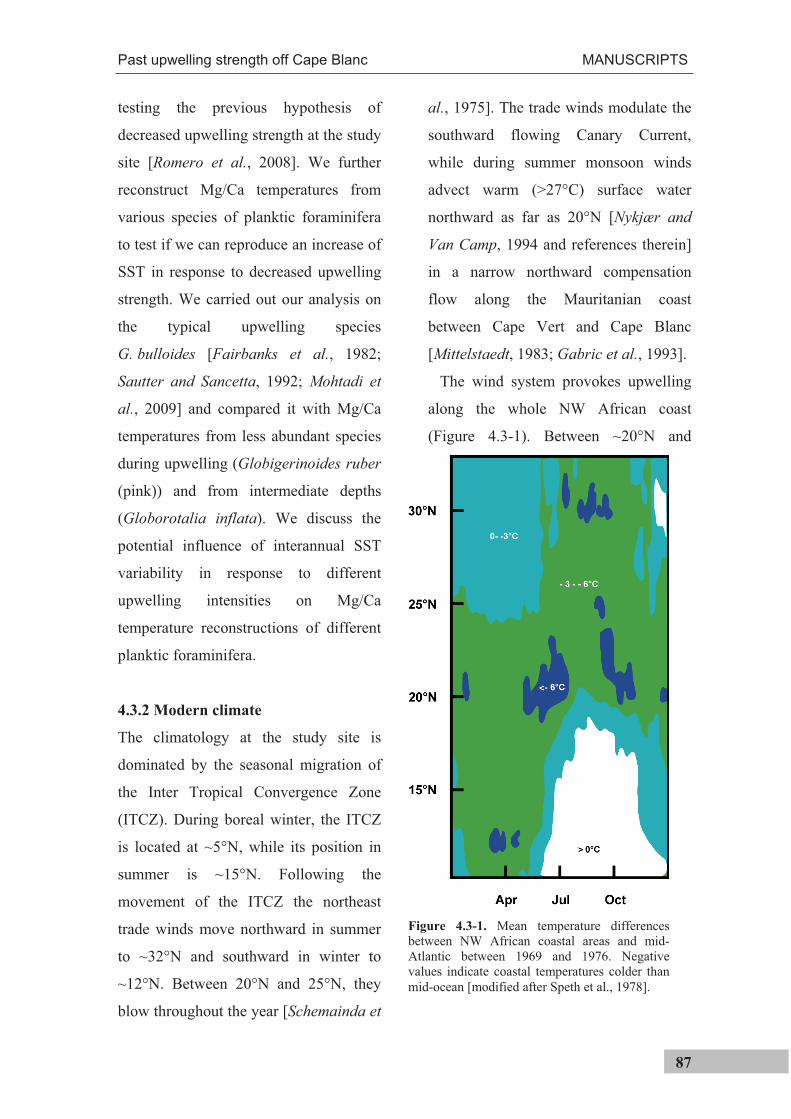
Past upwelling strength off Cape Blanc MANUSCRIPTS
87
testing the previous hypothesis of
decreased upwelling strength at the study
site [Romero et al., 2008]. We further
reconstruct Mg/Ca temperatures from
various species of planktic foraminifera
to test if we can reproduce an increase of
SST in response to decreased upwelling
strength. We carried out our analysis on
the typical upwelling species
G. bulloides [Fairbanks et al., 1982;
Sautter and Sancetta, 1992; Mohtadi et
al., 2009] and compared it with Mg/Ca
temperatures from less abundant species
during upwelling (Globigerinoides ruber
(pink)) and from intermediate depths
(Globorotalia inflata). We discuss the
potential influence of interannual SST
variability in response to different
upwelling intensities on Mg/Ca
temperature reconstructions of different
planktic foraminifera.
4.3.2 Modern climate
The climatology at the study site is
dominated by the seasonal migration of
the Inter Tropical Convergence Zone
(ITCZ). During boreal winter, the ITCZ
is located at ~5°N, while its position in
summer is ~15°N. Following the
movement of the ITCZ the northeast
trade winds move northward in summer
to ~32°N and southward in winter to
~12°N. Between 20°N and 25°N, they
blow throughout the year [Schemainda et
al., 1975]. The trade winds modulate the
southward flowing Canary Current,
while during summer monsoon winds
advect warm (>27°C) surface water
northward as far as 20°N [Nykjær and
Van Camp, 1994 and references therein]
in a narrow northward compensation
flow along the Mauritanian coast
between Cape Vert and Cape Blanc
[Mittelstaedt, 1983; Gabric et al., 1993].
The wind system provokes upwelling
along the whole NW African coast
(Figure 4.3-1). Between ~20°N and
Figure 4.3-1. Mean temperature differences
between NW African coastal areas and mid-
Atlantic between 1969 and 1976. Negative
values indicate coastal temperatures colder than
mid-ocean [modified after Speth et al., 1978].
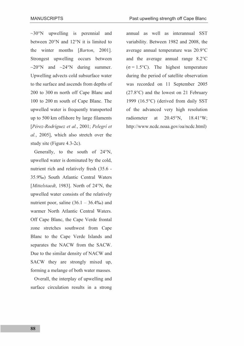
MANUSCRIPTS Past upwelling strength off Cape Blanc
88
~30°N upwelling is perennial and
between 20°N and 12°N it is limited to
the winter months [Barton, 2001].
Strongest upwelling occurs between
~20°N and ~24°N during summer.
Upwelling advects cold subsurface water
to the surface and ascends from depths of
200 to 300 m north off Cape Blanc and
100 to 200 m south of Cape Blanc. The
upwelled water is frequently transported
up to 500 km offshore by large filaments
[Pérez-Rodríguez et al., 2001; Pelegrí et
al., 2005], which also stretch over the
study site (Figure 4.3-2c).
Generally, to the south of 24°N,
upwelled water is dominated by the cold,
nutrient rich and relatively fresh (35.6 -
35.9‰) South Atlantic Central Waters
[Mittelstaedt, 1983]. North of 24°N, the
upwelled water consists of the relatively
nutrient poor, saline (36.1 – 36.4‰) and
warmer North Atlantic Central Waters.
Off Cape Blanc, the Cape Verde frontal
zone stretches southwest from Cape
Blanc to the Cape Verde Islands and
separates the NACW from the SACW.
Due to the similar density of NACW and
SACW they are strongly mixed up,
forming a melange of both water masses.
Overall, the interplay of upwelling and
surface circulation results in a strong
annual as well as interannual SST
variability. Between 1982 and 2008, the
average annual temperature was 20.9°C
and the average annual range 8.2°C
( = 1.5°C). The highest temperature
during the period of satellite observation
was recorded on 11 September 2005
(27.8°C) and the lowest on 21 February
1999 (16.5°C) (derived from daily SST
of the advanced very high resolution
radiometer at 20.45°N, 18.41°W;
http://www.ncdc.noaa.gov/oa/ncdc.html)
Past upwelling strength off Cape Blanc MANUSCRIPTS
89
Figure 4.3-2. Map of the study site with simplified atmospheric and oceanographic features. a) Monthly
SST during March is shown by color shading [Locarnini et al., 2006]. Red lines show 72h backward (to the
north) and forward (to the south) wind trajectories in March moving at 100 m above the study site during
the year 2000 (Calculated using the Hybrid single particle Lagrangian Trajectory Model of the National
Oceanic and Atmospheric Administration Air resources laboratory; http://ready.arl.noaa.gov/hysplit-
bin/trajtype.pl?runtype=archive). Red numbers in boxes indicate respective day of the month. b) same as (a)
but for September c) Chlorophyll a concentration between 22 and 29 September 2005
(http://oceancolor.gsfc.nasa.gov/).
4.3.3 Material and methods
Sample collection and revised age
model
The 1330 cm long gravity core
GeoB7926-2 was recovered during R/V
Meteor Cruise 53/1c [Meggers and
cruise participants, 2003] at 20°12.8’N,
18°27.1’W at 2500 m water depth.
Samples representative for present day
were collected from the top centimeter of
multicore GeoB 7408-2 at 20°17.4’N,
18°15.0’W, recovered in a water depth
of 1935 m, during R/V Poseidon cruise
272 [Meggers et al., 2002], less than
13 nm away from the gravity core.
Sediment samples were wet-sieved into
the two size fractions of 63-150 µm and
>150 µm.
The age model of the upper 820 cm is
based on 12 Accelerator Mass
Spectrometry (AMS) 14
C dates on
monospecific samples of the planktic
foraminifera G. inflata and covers
approximately the last 24 kyrs.
Radiocarbon ages have been previously
published [Romero et al., 2008]. We
revised the age model, converting
radiocarbon ages into calendar years
using the Calib Rev 6.1.0 program, with
the most recent marine calibration
dataset marine09.14c [Reimer et al.,
2009]. We acknowledge that the dated
species G. inflata was possibly exposed
to water exceeding the global reservoir
age of ~400 yrs. We hence calculated the
MANUSCRIPTS Past upwelling strength off Cape Blanc
90
calendar age that would be associated
with an additional local reservoir age of
197 years ( R). This is the local
reservoir age further south
(http://www.calib.qub.ac.uk/marine/regi
oncalc.php), where old South Atlantic
Central Water is upwelled, likely
exhibiting the oldest reservoir age at the
study site. In Table 4.3-1, we show
calculated calendar ages assuming no
reservoir age and in Table 4.3-2
assuming a R of 197 years to show the
effect this has on the calculated calendar
ages.
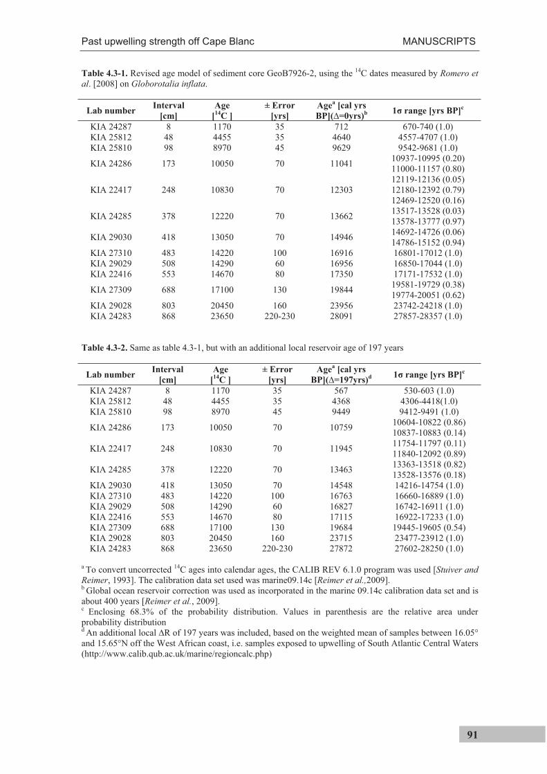
Past upwelling strength off Cape Blanc MANUSCRIPTS
91
Table 4.3-1. Revised age model of sediment core GeoB7926-2, using the 14C dates measured by Romero et al. [2008] on Globorotalia inflata.
Lab number Interval
[cm]
Age
[14
C ]
± Error
[yrs]
Agea [cal yrs
BP]( =0yrs)b 1 range [yrs BP]
c
KIA 24287 8 1170 35 712 670-740 (1.0)
KIA 25812 48 4455 35 4640 4557-4707 (1.0)
KIA 25810 98 8970 45 9629 9542-9681 (1.0)
KIA 24286 173 10050 70 11041 10937-10995 (0.20)
11000-11157 (0.80)
KIA 22417 248 10830 70 12303
12119-12136 (0.05)
12180-12392 (0.79)
12469-12520 (0.16)
KIA 24285 378 12220 70 13662 13517-13528 (0.03)
13578-13777 (0.97)
KIA 29030 418 13050 70 14946 14692-14726 (0.06)
14786-15152 (0.94)
KIA 27310 483 14220 100 16916 16801-17012 (1.0)
KIA 29029 508 14290 60 16956 16850-17044 (1.0)
KIA 22416 553 14670 80 17350 17171-17532 (1.0)
KIA 27309 688 17100 130 19844 19581-19729 (0.38)
19774-20051 (0.62)
KIA 29028 803 20450 160 23956 23742-24218 (1.0)
KIA 24283 868 23650 220-230 28091 27857-28357 (1.0)
Table 4.3-2. Same as table 4.3-1, but with an additional local reservoir age of 197 years
Lab number Interval
[cm]
Age
[14
C ]
± Error
[yrs]
Agea [cal yrs
BP]( =197yrs)d 1 range [yrs BP]
c
KIA 24287 8 1170 35 567 530-603 (1.0)
KIA 25812 48 4455 35 4368 4306-4418(1.0)
KIA 25810 98 8970 45 9449 9412-9491 (1.0)
KIA 24286 173 10050 70 10759 10604-10822 (0.86)
10837-10883 (0.14)
KIA 22417 248 10830 70 11945 11754-11797 (0.11)
11840-12092 (0.89)
KIA 24285 378 12220 70 13463 13363-13518 (0.82)
13528-13576 (0.18)
KIA 29030 418 13050 70 14548 14216-14754 (1.0)
KIA 27310 483 14220 100 16763 16660-16889 (1.0)
KIA 29029 508 14290 60 16827 16742-16911 (1.0)
KIA 22416 553 14670 80 17115 16922-17233 (1.0)
KIA 27309 688 17100 130 19684 19445-19605 (0.54)
KIA 29028 803 20450 160 23715 23477-23912 (1.0)
KIA 24283 868 23650 220-230 27872 27602-28250 (1.0)
a To convert uncorrected 14C ages into calendar ages, the CALIB REV 6.1.0 program was used [Stuiver and Reimer, 1993]. The calibration data set used was marine09.14c [Reimer et al.,2009]. b Global ocean reservoir correction was used as incorporated in the marine 09.14c calibration data set and is
about 400 years [Reimer et al., 2009]. c Enclosing 68.3% of the probability distribution. Values in parenthesis are the relative area under
probability distribution d An additional local R of 197 years was included, based on the weighted mean of samples between 16.05°
and 15.65°N off the West African coast, i.e. samples exposed to upwelling of South Atlantic Central Waters
(http://www.calib.qub.ac.uk/marine/regioncalc.php)
MANUSCRIPTS Past upwelling strength off Cape Blanc
92
Data acquisition
Mg/Ca thermometry
All species were identified following the
taxonomy of Hemleben et al. [1989].
Most G. inflata (d’Orbigny) specimens
had four chambers in the last whorl, and
had moderately thickened walls.
Between 14 and 30 specimens of
G. bulloides, 14-28 specimens of
G. ruber (pink) and ~20 specimens of
G. inflata were gently crushed and
cleaned according to the Barker et al.
[2003] protocol. G. inflata sizes were
mostly between 400 and 480 µm, while
for G. bulloides and G. ruber (pink)
somewhat large size ranges (listed in
Table 4.3-S1) were necessary in order to
collect enough specimens for analysis.
Uncertainties related to these are
addressed in the discussion section.
Samples were washed seven times with
suprapure (18.2 M cm) water, twice
with methanol followed by two oxidation
steps of 10 min and a weak acid leach in
0.001M TD HNO3. Samples were
dissolved in 0.075M TD HNO3,
centrifuged for 10 min at 6000 rpm,
transferred into test tubes and diluted for
analysis. Mg/Ca ratios were measured
with a Perkin Elmer Optima 3300R
Inductively Coupled Plasma Optical
Emission Spectrometer (ICP-OES)
equipped with an auto sampler and an
ultrasonic nebulizer U-5000 AT (Cetac
Technologies Inc.) and with an Agilent
Technologies 700 Series ICP-OES, at the
faculty of Geosciences and the Center
for Marine Environmental Sciences,
University of Bremen. Verification of
the Mg/Ca ratios was achieved against
international carbonate reference
material ECRM 752-1 [Greaves et al.,
2008]. The Mg/Ca ratio of the standard
during the analytical sessions for
G. bulloides and G. ruber (pink) was on
average 3.84 mmol/mol (n = 21,
= ±0.02 mmol/mol) and during the
analysis of G. inflata on average
3.84 mmol/mol (n = 12;
= ±0.04 mmol/mol). Stability of the
Mg/Ca measurements was monitored by
analysis of an in-house artificial standard
solution with Mg/Ca ratio of
2.95 mmol/mol (n = 35;
= ±0.02 mmol/mol) during the
analytical session for G. bulloides and
G. ruber (pink) and 3.01 mmol/mol
(n = 40; = ±0.05 mmol/mol) during the
analytical session for G. inflata. The
precision of Mg/Ca measurements on
G. bulloides and G. ruber (pink) was on
average 0.09%, based on three replicates
(n=120) and the precision of Mg/Ca
measurements on G. inflata on average
0.22%, based on mostly three (n=111)
and few times (n=17) two replicates. In
order to correct for small shifts between
Past upwelling strength off Cape Blanc MANUSCRIPTS
93
analytical sessions, values of individual
sessions were normalized to the reported
Mg/Ca ratio of 3.75 mmol/mol of the
ECRM 752-1 [Greaves et al., 2008].
Samples did not show visible
encrustations or dissolution in light
microscopic inspection. Core depths with
suspiciously high Mg/Ca were resampled
for G. ruber (pink) and G. bulloides and
specimens were subjected to SEM
inspection, which did not show signs of
diagenesis (Figure 4.3-4).
For calculating the Mg/Ca
temperatures of G. bulloides (equation
4.3-1) and G. inflata (equation 4.3-2) the
calibration equations of Elderfield and
Ganssen [2000] were used.
T = ln ((Mg/Ca)/0.56))/0.1 (4.3-1)
T = ln ((Mg/Ca))/0.49)/0.1 (4.3-2)
For calculating the G. ruber (pink)
calcification temperature, the equation of
Regenberg et al. [2009] was used.
T = ln ((Mg/Ca)/0.87))/0.056 (4.3-3)
The selection of these equations from a
substantial number of calibrations was
based on the following considerations.
For G. ruber (pink) and G. inflata these
equations gave the most realistic
estimates in a sediment trap study just
above the core location [Haarmann et
al., 2011]. For G. bulloides, the use of
the Elderfield and Ganssen [2000]
equation gives a SST of 19.0°C for the
most recent sample, in good agreement
with the average SST during the times of
main flux [B. Donner, pers. comm.] at
the study site (18.8°C in March and
20.3°C in July).
G. bulloides census counts
Sediment samples were divided into
aliquots using a MS-1 microsplitter of
ASC scientific and contained at least 300
specimens of planktic foraminifera.
G. bulloides percentage was then
calculated relative to the total fauna.
MANUSCRIPTS Past upwelling strength off Cape Blanc
94
4.3.4 Results
G. bulloides census count
The relative abundance of G. bulloides
ranges between 32 % (22.1 kyrs BP) and
4.5 % (2.5 kyrs BP) (Figure 4.3-3b).
During the LGM and Heinrich Stadial 1
(HS1) between 23.6 kyrs BP and
15.6 kyrs BP, G. bulloides abundances
are high and on average 18.4 %. This
period is followed by a sharp decrease
within about 300 years after HS1.
Throughout Bølling-Allerød (B/A),
Younger Dryas (YD) and the major part
of the Holocene until 3.4 kyrs BP,
abundances remain at a moderate level
and are on average 12.2 %. After
3.4 kyrs BP until present, values are low
and on average 5 %.
Comparison of our results to the study
of Adkins et al. [2006] shows that the
deglacial as well as Holocene values of
G. bulloides abundances are much lower
than in the nearby core ODP 658C
(~40 % and ~15 %), with an earlier
Holocene decrease than observed in core
ODP685C (~5.5 kyrs BP). The
G. bulloides abundances are closer to
values from sediment core GIK 12310-4
[Diester-Haass et al., 1973], which were
~30 % during the last deglacial, and
sharply decreased between 10.4 kyrs BP
and 9.2 kyrs BP to values of ~20 %.
Mg/Ca paleothermometry
G. ruber (pink) and G. bulloides
Mg/Ca ratios of G. bulloides range
between 2.32 and 6.87 mmol/mol. Using
the Mg/Ca temperature calibration of
Elderfield and Ganssen [2000] this
corresponds to temperatures between
14.2°C (16.0 kyrs BP) and 25.1°C
(16.8 kyrs BP). No trend is discernable
throughout the last 24 kyrs. During the
LGM, between 23.2 kyrs BP and
19.1 kyrs BP, temperatures were on
average 18.1°C. Between 19.1 kyrs BP
and 15.7 kyrs BP, temperatures are
slightly higher with two marked
temperature maxima at 18.9 kyrs BP
(23.7°C) and 16.8 kyrs BP (25.1°C).
During the B/A interstadial, no clear
temperature trend is observed, while
during the YD, SSTs were slightly
higher compared to the BA. The average
temperature throughout the Holocene
was 18°C.
Mg/Ca ratios of G. ruber (pink) range
between 2.56 and 4.53 mmol/mol. Using
the Mg/Ca temperature calibration of
Regenberg et al. [2009] this corresponds
to temperatures between 16.6°C
(11.4 kyrs BP) and 25.4°C (16.9 kyrs
BP). During the LGM, between
22.8 kyrs BP and 19.1 kyrs BP,
temperatures were on average 19.3°C.
Between 19.1 and 16.0 kyrs BP, SST
Past upwelling strength off Cape Blanc MANUSCRIPTS
95
was episodically high with a maximum
increase of 7.7°C (25.3°C) compared to
the LGM. During the B/A between
13.5 kyrs and 12.8 kyrs BP temperatures
reach peak values of 24.9°C and 24.4°C,
respectively. A negative anomaly is
centered at 11.4 kyrs BP (16.6°C).
Throughout the Holocene, temperatures
averaged 20°C and varied much less than
during the last deglacial (maximal
2.8°C).
G. inflata
The minimum Mg/Ca ratio of G.inflata
is 1.41 mmol/mol at 1.5 kyrs BP. Using
the calibration equation of Elderfield and
Ganssen [2000], this corresponds to a
temperature of 10.6°C. A maximum of
4.08 mmol/mol is reached at 9.9 kyrs BP
(21.2°C). Between 23.5 and
22.2 kyrs BP, Mg/Ca ratios sharply
decrease from 3.59 mmol/mol to
1.52 mmol/mol (19.9°C to 11.3°C). This
is followed by a gradual increase to
4.08 mmol/mol (21.2°C) (9.9kyrs BP).
Mg/Ca ratios then decrease again to a
value of 1.41 mmol/mol (10.6°C) at
1.5 kyrs BP, before reaching their
present day value of 2.25 mmol/mol
(15.2°C).
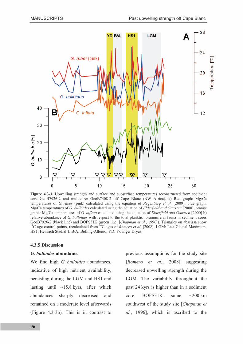
MANUSCRIPTS Past upwelling strength off Cape Blanc
96
Figure 4.3-3. Upwelling strength and surface and subsurface temperatures reconstructed from sediment
core GeoB7926-2 and multicorer GeoB7408-2 off Cape Blanc (NW Africa). a) Red graph: Mg/Ca
temperatures of G. ruber (pink) calculated using the equation of Regenberg et al. [2009]; blue graph:
Mg/Ca temperatures of G. bulloides calculated using the equation of Elderfield and Ganssen [2000]; orange
graph: Mg/Ca temperatures of G. inflata calculated using the equation of Elderfield and Ganssen [2000] b)
relative abundance of G. bulloides with respect to the total planktic foraminiferal fauna in sediment cores
GeoB7926-2 (black line) and BOFS31K (green line, [Chapman et al., 1996]). Triangles on abscissa show 14C age control points, recalculated from 14C ages of Romero et al. [2008]. LGM: Last Glacial Maximum,
HS1: Heinrich Stadial 1, B/A: Bølling-Allerød, YD: Younger Dryas.
4.3.5 Discussion
G. bulloides abundance
We find high G. bulloides abundances,
indicative of high nutrient availability,
persisting during the LGM and HS1 and
lasting until ~15.8 kyrs, after which
abundances sharply decreased and
remained on a moderate level afterwards
(Figure 4.3-3b). This is in contrast to
previous assumptions for the study site
[Romero et al., 2008] suggesting
decreased upwelling strength during the
LGM. The variability throughout the
past 24 kyrs is higher than in a sediment
core BOFS31K some ~200 km
southwest of the study site [Chapman et
al., 1996], which is ascribed to the
Past upwelling strength off Cape Blanc MANUSCRIPTS
97
position of the sediment core studies
here just below the large upwelling
filament. There, a large degree of
variability with respect to the offshore
export of nutrients is observed on short
(daily) as well as long (interannual)
timescales [Gabric et al., 1993].
The decrease after ~15.8 kyrs BP
coincides with a strong decrease in wind
strength between ~16 and 12 kyrs BP
reconstructed ~150 km north of the study
site [Martinez et al., 1999]. This argues
for a control of wind strength on nutrient
availability and does not support the
assumption of decreased upwelling
through an increase of easterly
(continental) winds [Zhao et al., 2000]. It
is rather in line with previous studies that
suggest the strength of northeasterly
trade winds controls productivity off
Cape Blanc through its influence on the
extension of the upwelling cell
[Chapman et al., 1996] and a greater
offshore movement of upwelled waters
by wind-induced advection and
diffusion.
Mg/Ca temperatures
Reconstructed Mg/Ca temperatures
cannot be clearly assigned to any of the
major rapid climatic changes since the
LGM. No substantial cooling was
reconstructed for the LGM, HS1 or the
YD in all species (Figure 4.3-3a) nor
reconstructed during the period of strong
upwelling as suggested by high
G. bulloides abundances (Figure 4.3-3b)
between the LGM and 15.8 kyrs BP.
Rather, high Mg/Ca ratios and
consequently high temperatures are
recorded by the surface dwelling species
during this period and in particular
during HS1.
Possible influences on the Mg/Ca
ratios
Mg/Ca ratios in foraminifera can be
biased by a number of factors other than
temperature, that comprise
contamination with clay minerals
[Barker et al., 2003], dissolution [e.g.;
Benway et al., 2003] or secondary calcite
addition [e.g.; Groeneveld and Chiessi,
2011], size related effects [e.g.;
Elderfield et al., 2002] and salinity [e.g.
Ferguson et al., 2008; Kisakürek et al.,
2008; Arbuszewski et al., 2010].
Clay minerals contain between ~1 and
~10% Mg by weight [Deer et al., 1992],
and can therefore bias Mg/Ca
determinations towards higher values
than that of pristine foraminiferal calcite.
Cleaning of the shells was carried out
following the well established Barker et
al. [2003] protocol that included steps
for clay removal. Parallel to
determination of Mg concentrations, Fe
concentrations were measured. In our
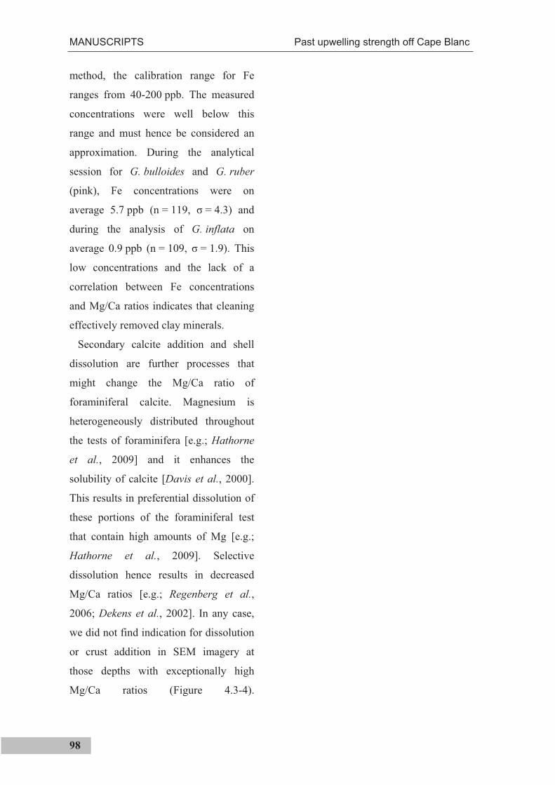
MANUSCRIPTS Past upwelling strength off Cape Blanc
98
method, the calibration range for Fe
ranges from 40-200 ppb. The measured
concentrations were well below this
range and must hence be considered an
approximation. During the analytical
session for G. bulloides and G. ruber
(pink), Fe concentrations were on
average 5.7 ppb (n = 119, = 4.3) and
during the analysis of G. inflata on
average 0.9 ppb (n = 109, = 1.9). This
low concentrations and the lack of a
correlation between Fe concentrations
and Mg/Ca ratios indicates that cleaning
effectively removed clay minerals.
Secondary calcite addition and shell
dissolution are further processes that
might change the Mg/Ca ratio of
foraminiferal calcite. Magnesium is
heterogeneously distributed throughout
the tests of foraminifera [e.g.; Hathorne
et al., 2009] and it enhances the
solubility of calcite [Davis et al., 2000].
This results in preferential dissolution of
these portions of the foraminiferal test
that contain high amounts of Mg [e.g.;
Hathorne et al., 2009]. Selective
dissolution hence results in decreased
Mg/Ca ratios [e.g.; Regenberg et al.,
2006; Dekens et al., 2002]. In any case,
we did not find indication for dissolution
or crust addition in SEM imagery at
those depths with exceptionally high
Mg/Ca ratios (Figure 4.3-4).
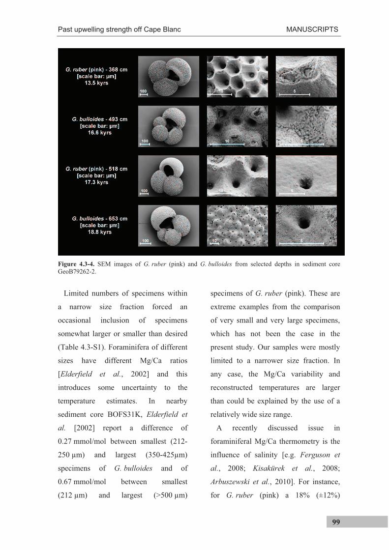
Past upwelling strength off Cape Blanc MANUSCRIPTS
99
Figure 4.3-4. SEM images of G. ruber (pink) and G. bulloides from selected depths in sediment core
GeoB79262-2.
Limited numbers of specimens within
a narrow size fraction forced an
occasional inclusion of specimens
somewhat larger or smaller than desired
(Table 4.3-S1). Foraminifera of different
sizes have different Mg/Ca ratios
[Elderfield et al., 2002] and this
introduces some uncertainty to the
temperature estimates. In nearby
sediment core BOFS31K, Elderfield et
al. [2002] report a difference of
0.27 mmol/mol between smallest (212-
250 µm) and largest (350-425µm)
specimens of G. bulloides and of
0.67 mmol/mol between smallest
(212 µm) and largest (>500 µm)
specimens of G. ruber (pink). These are
extreme examples from the comparison
of very small and very large specimens,
which has not been the case in the
present study. Our samples were mostly
limited to a narrower size fraction. In
any case, the Mg/Ca variability and
reconstructed temperatures are larger
than could be explained by the use of a
relatively wide size range.
A recently discussed issue in
foraminiferal Mg/Ca thermometry is the
influence of salinity [e.g. Ferguson et
al., 2008; Kisakürek et al., 2008;
Arbuszewski et al., 2010]. For instance,
for G. ruber (pink) a 18% (±12%)
MANUSCRIPTS Past upwelling strength off Cape Blanc
100
Mg/Ca increase per psu is reported
[Ferguson et al., 2008] and for G. ruber
(white) and exponential increase of 5%
(±3%) [Kisakürek et al., 2008]. Such
dependency would affect Mg/Ca
temperature determinations at the study
site, considering recent studies
suggesting a salinity increase of ~2.5 psu
along the NW African margin during the
LGM [Huang et al., submitted]. Taking
the Mg/Ca-salinity relationship of
Ferguson et al. [2008] at face value, this
could account for a ~45% increase of the
Mg/Ca ratio in G. ruber (pink) during
the LGM and HS1. If a substantial
advection of salty North Atlantic Central
Waters impaired the Mg/Ca ratios of
G. ruber (pink) and G. bulloides, it is
then surprising that this did not affect the
intermediate depth dwelling species
G. inflata, which lives in the same water
mass. It is therefore assumed that another
mechanism must have caused the large
variability recorded by the surface
dwelling species in contrast to the
intermediate depth dwelling species
G. inflata. We propose that this is the
large SST variability at the study site,
both on short (daily/weekly) as well as
long (interannual) timescales.
Modern SST variability and upwelling
strength
Present day satellite observations reveal
substantial interannual SST variability at
the study site. Figure 4.3-5 shows the
range of daily SSTs during November
(main flux period of G. ruber (pink) and
weak upwelling period; conf. section
4.3.2) between 1982 and 2008. SST
variability is generally high, while
during some years (e.g.; 2000) daily
SSTs exhibit a narrow range during
November. However, this can be
substantially different in the following or
preceding years (e.g.; 2001 and 1999 in
this example). We note that a change of
wind strength/upwelling strength does
not influence the overall high SST
variability in this example that represents
the non-upwelling period (November).
Figure 4.3-5 also shows the range of
daily SSTs during July (main flux period
of G. bulloides and main upwelling
period; conf. section 4.3.2). Notably,
during the period of weak wind stress,
temperatures exhibit a reasonably small
range and little variability. With the
onset of higher wind stress, temperature
variability becomes substantially more
pronounced. Most remarkably, higher
wind stress does not lead to negative
temperature anomalies at the study site,
as would be expected through stronger
upwelling. Rather, exceptionally high
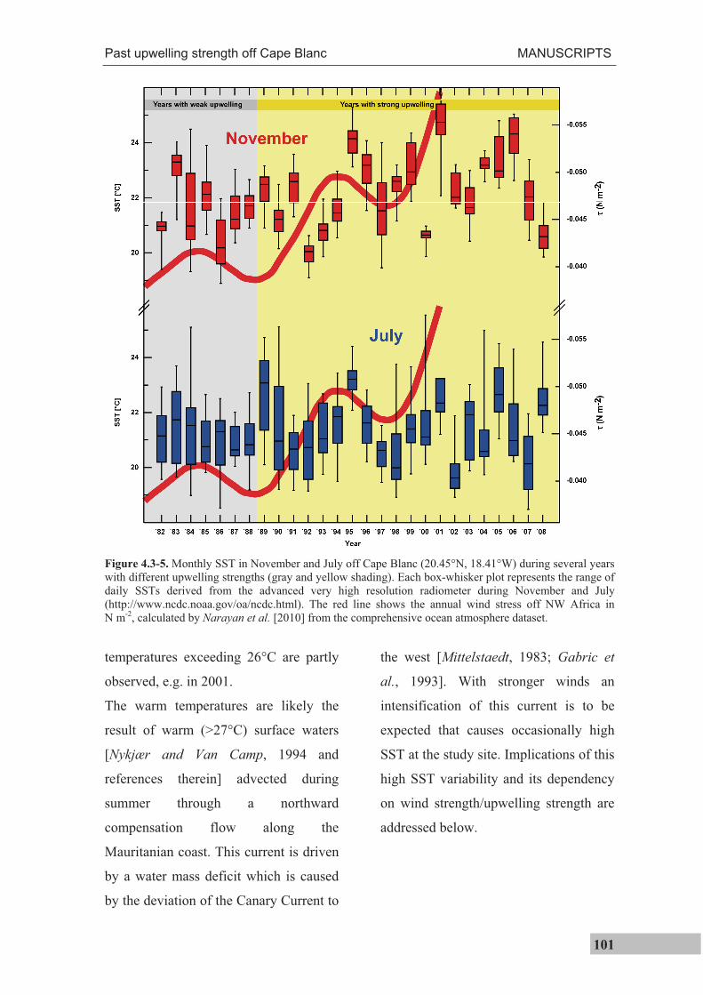
Past upwelling strength off Cape Blanc MANUSCRIPTS
101
Figure 4.3-5. Monthly SST in November and July off Cape Blanc (20.45°N, 18.41°W) during several years
with different upwelling strengths (gray and yellow shading). Each box-whisker plot represents the range of
daily SSTs derived from the advanced very high resolution radiometer during November and July
(http://www.ncdc.noaa.gov/oa/ncdc.html). The red line shows the annual wind stress off NW Africa in
N m-2, calculated by Narayan et al. [2010] from the comprehensive ocean atmosphere dataset.
temperatures exceeding 26°C are partly
observed, e.g. in 2001.
The warm temperatures are likely the
result of warm (>27°C) surface waters
[Nykjær and Van Camp, 1994 and
references therein] advected during
summer through a northward
compensation flow along the
Mauritanian coast. This current is driven
by a water mass deficit which is caused
by the deviation of the Canary Current to
the west [Mittelstaedt, 1983; Gabric et
al., 1993]. With stronger winds an
intensification of this current is to be
expected that causes occasionally high
SST at the study site. Implications of this
high SST variability and its dependency
on wind strength/upwelling strength are
addressed below.
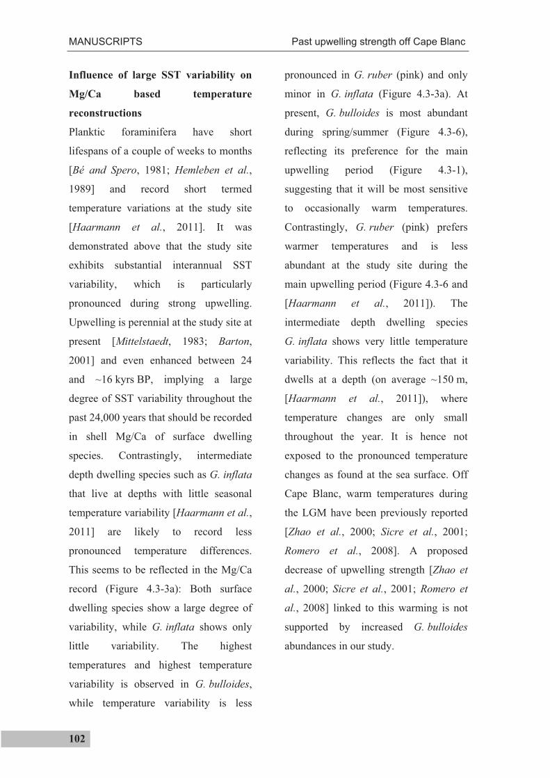
MANUSCRIPTS Past upwelling strength off Cape Blanc
102
Influence of large SST variability on
Mg/Ca based temperature
reconstructions
Planktic foraminifera have short
lifespans of a couple of weeks to months
[Bé and Spero, 1981; Hemleben et al.,
1989] and record short termed
temperature variations at the study site
[Haarmann et al., 2011]. It was
demonstrated above that the study site
exhibits substantial interannual SST
variability, which is particularly
pronounced during strong upwelling.
Upwelling is perennial at the study site at
present [Mittelstaedt, 1983; Barton,
2001] and even enhanced between 24
and ~16 kyrs BP, implying a large
degree of SST variability throughout the
past 24,000 years that should be recorded
in shell Mg/Ca of surface dwelling
species. Contrastingly, intermediate
depth dwelling species such as G. inflata
that live at depths with little seasonal
temperature variability [Haarmann et al.,
2011] are likely to record less
pronounced temperature differences.
This seems to be reflected in the Mg/Ca
record (Figure 4.3-3a): Both surface
dwelling species show a large degree of
variability, while G. inflata shows only
little variability. The highest
temperatures and highest temperature
variability is observed in G. bulloides,
while temperature variability is less
pronounced in G. ruber (pink) and only
minor in G. inflata (Figure 4.3-3a). At
present, G. bulloides is most abundant
during spring/summer (Figure 4.3-6),
reflecting its preference for the main
upwelling period (Figure 4.3-1),
suggesting that it will be most sensitive
to occasionally warm temperatures.
Contrastingly, G. ruber (pink) prefers
warmer temperatures and is less
abundant at the study site during the
main upwelling period (Figure 4.3-6 and
[Haarmann et al., 2011]). The
intermediate depth dwelling species
G. inflata shows very little temperature
variability. This reflects the fact that it
dwells at a depth (on average ~150 m,
[Haarmann et al., 2011]), where
temperature changes are only small
throughout the year. It is hence not
exposed to the pronounced temperature
changes as found at the sea surface. Off
Cape Blanc, warm temperatures during
the LGM have been previously reported
[Zhao et al., 2000; Sicre et al., 2001;
Romero et al., 2008]. A proposed
decrease of upwelling strength [Zhao et
al., 2000; Sicre et al., 2001; Romero et
al., 2008] linked to this warming is not
supported by increased G. bulloides
abundances in our study.
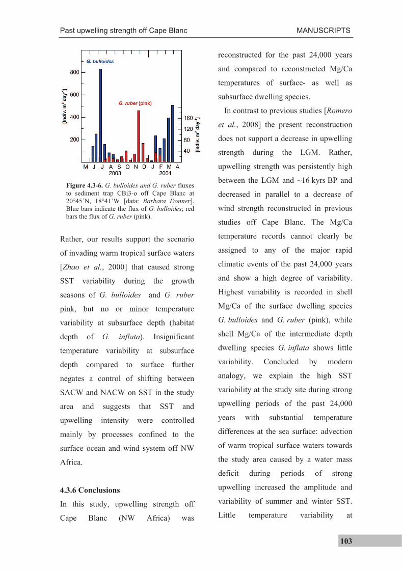
Past upwelling strength off Cape Blanc MANUSCRIPTS
103
Figure 4.3-6. G. bulloides and G. ruber fluxes
to sediment trap CBi3-o off Cape Blanc at
20°45’N, 18°41’W [data: Barbara Donner].
Blue bars indicate the flux of G. bulloides; red
bars the flux of G. ruber (pink).
Rather, our results support the scenario
of invading warm tropical surface waters
[Zhao et al., 2000] that caused strong
SST variability during the growth
seasons of G. bulloides and G. ruber
pink, but no or minor temperature
variability at subsurface depth (habitat
depth of G. inflata). Insignificant
temperature variability at subsurface
depth compared to surface further
negates a control of shifting between
SACW and NACW on SST in the study
area and suggests that SST and
upwelling intensity were controlled
mainly by processes confined to the
surface ocean and wind system off NW
Africa.
4.3.6 Conclusions
In this study, upwelling strength off
Cape Blanc (NW Africa) was
reconstructed for the past 24,000 years
and compared to reconstructed Mg/Ca
temperatures of surface- as well as
subsurface dwelling species.
In contrast to previous studies [Romero
et al., 2008] the present reconstruction
does not support a decrease in upwelling
strength during the LGM. Rather,
upwelling strength was persistently high
between the LGM and ~16 kyrs BP and
decreased in parallel to a decrease of
wind strength reconstructed in previous
studies off Cape Blanc. The Mg/Ca
temperature records cannot clearly be
assigned to any of the major rapid
climatic events of the past 24,000 years
and show a high degree of variability.
Highest variability is recorded in shell
Mg/Ca of the surface dwelling species
G. bulloides and G. ruber (pink), while
shell Mg/Ca of the intermediate depth
dwelling species G. inflata shows little
variability. Concluded by modern
analogy, we explain the high SST
variability at the study site during strong
upwelling periods of the past 24,000
years with substantial temperature
differences at the sea surface: advection
of warm tropical surface waters towards
the study area caused by a water mass
deficit during periods of strong
upwelling increased the amplitude and
variability of summer and winter SST.
Little temperature variability at
MANUSCRIPTS Past upwelling strength off Cape Blanc
104
subsurface depths suggests negligible
contribution of NACW and SACW to
SST changes in the study area
throughout the past 24,000 years.
Acknowledgements
Sample collection and technical support was
provided by The Center for Marine
Environmental Sciences (MARUM),
University of Bremen. We thank Petra Witte
for SEM imaging and Barbara Donner for
providing unpublished data. This study was
carried out within the International Graduate
College EUROPROX, funded by the
Deutsche Forschungsgemeinschaft (DFG).
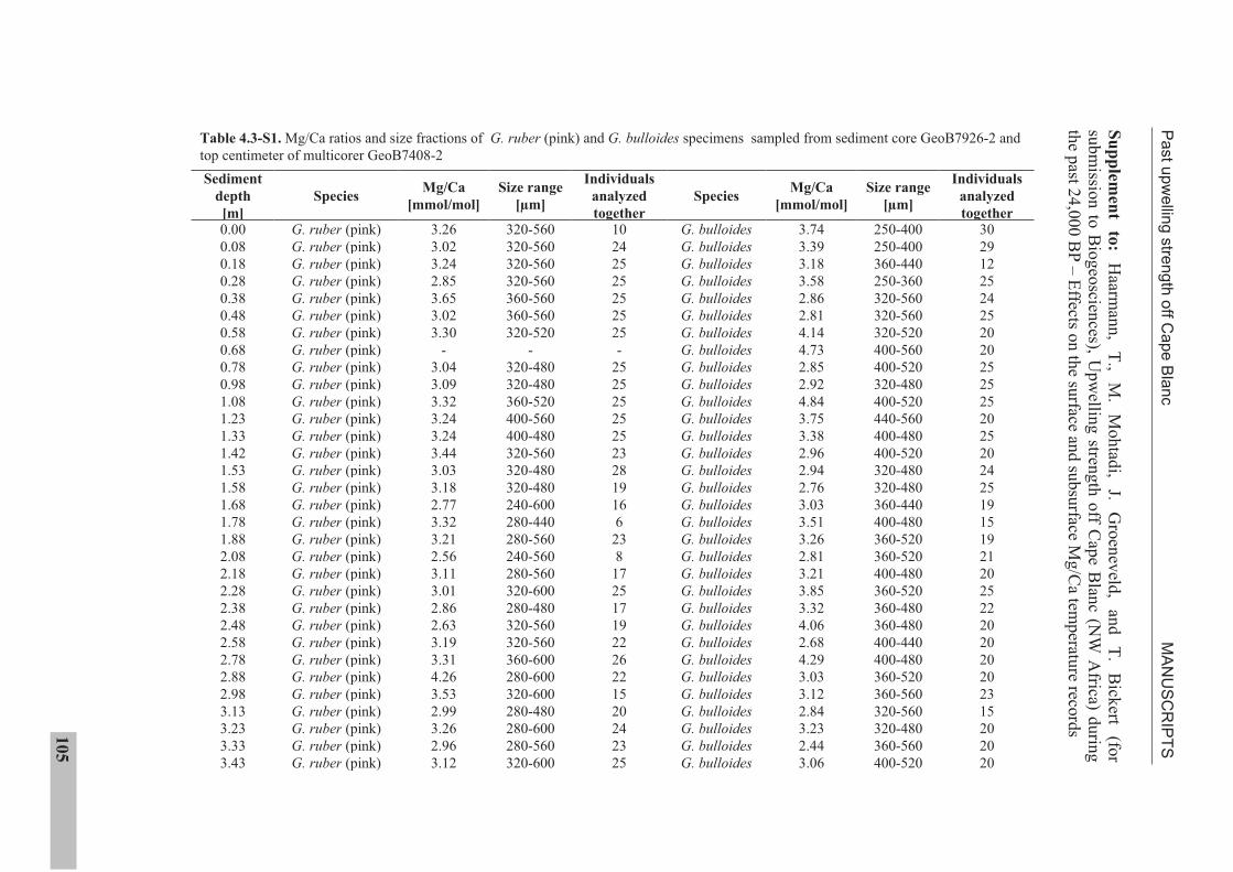
Pa
st u
pw
ellin
g s
tren
gth
off C
ap
e B
lan
c M
AN
US
CR
IPT
S
105
Su
pp
lemen
t to
:H
aarman
n,
T.,
M.
Mohtad
i, J.
Gro
enev
eld,
and
T.
Bick
ert (fo
r
subm
ission
to B
iog
eoscien
ces), Upw
elling stren
gth
off C
ape B
lanc (N
W A
frica) durin
g
the p
ast 24
,00
0 B
P –
Effects o
n th
e surface an
d su
bsu
rface Mg
/Ca tem
peratu
re record
s Individuals
analyzed
together30
29
12
25
24
25
20
20
25
25
25
20
25
20
24
25
19
15
19
21
20
25
22
20
20
20
20
23
15
20
20
20
Size range
[µm]
250-400
250-400
360-440
250-360
320-560
320-560
320-520
400-560
400-520
320-480
400-520
440-560
400-480
400-520
320-480
320-480
360-440
400-480
360-520
360-520
400-480
360-520
360-480
360-480
400-440
400-480
360-520
360-560
320-560
320-480
360-560
400-520
Mg/Ca
[mmol/mol]
3.74
3.39
3.18
3.58
2.86
2.81
4.14
4.73
2.85
2.92
4.84
3.75
3.38
2.96
2.94
2.76
3.03
3.51
3.26
2.81
3.21
3.85
3.32
4.06
2.68
4.29
3.03
3.12
2.84
3.23
2.44
3.06
Species
G. bulloides
G. bulloides
G. bulloides
G. bulloides
G. bulloides
G. bulloides
G. bulloides
G. bulloides
G. bulloides
G. bulloides
G. bulloides
G. bulloides
G. bulloides
G. bulloides
G. bulloides
G. bulloides
G. bulloides
G. bulloides
G. bulloides
G. bulloides
G. bulloides
G. bulloides
G. bulloides
G. bulloides
G. bulloides
G. bulloides
G. bulloides
G. bulloides
G. bulloides
G. bulloides
G. bulloides
G. bulloides
Individuals
analyzed
together10
24
25
25
25
25
25
-
25
25
25
25
25
23
28
19
16
6
23
8
17
25
17
19
22
26
22
15
20
24
23
25
Size range
[µm]
320-560
320-560
320-560
320-560
360-560
360-560
320-520
-
320-480
320-480
360-520
400-560
400-480
320-560
320-480
320-480
240-600
280-440
280-560
240-560
280-560
320-600
280-480
320-560
320-560
360-600
280-600
320-600
280-480
280-600
280-560
320-600
Mg/Ca
[mmol/mol]
3.26
3.02
3.24
2.85
3.65
3.02
3.30
-
3.04
3.09
3.32
3.24
3.24
3.44
3.03
3.18
2.77
3.32
3.21
2.56
3.11
3.01
2.86
2.63
3.19
3.31
4.26
3.53
2.99
3.26
2.96
3.12
Species
G. ruber (pink)
G. ruber (pink)
G. ruber (pink)
G. ruber (pink)
G. ruber (pink)
G. ruber (pink)
G. ruber (pink)
G. ruber (pink)
G. ruber (pink)
G. ruber (pink)
G. ruber (pink)
G. ruber (pink)
G. ruber (pink)
G. ruber (pink)
G. ruber (pink)
G. ruber (pink)
G. ruber (pink)
G. ruber (pink)
G. ruber (pink)
G. ruber (pink)
G. ruber (pink)
G. ruber (pink)
G. ruber (pink)
G. ruber (pink)
G. ruber (pink)
G. ruber (pink)
G. ruber (pink)
G. ruber (pink)
G. ruber (pink)
G. ruber (pink)
G. ruber (pink)
G. ruber (pink)
Table 4.3-S1. Mg/Ca ratios and size fractions of G. ruber (pink) and G. bulloides specimens sampled from sediment core GeoB7926-2 and
top centimeter of multicorer GeoB7408-2
Sediment
depth
[m]0.00
0.08
0.18
0.28
0.38
0.48
0.58
0.68
0.78
0.98
1.08
1.23
1.33
1.42
1.53
1.58
1.68
1.78
1.88
2.08
2.18
2.28
2.38
2.48
2.58
2.78
2.88
2.98
3.13
3.23
3.33
3.43
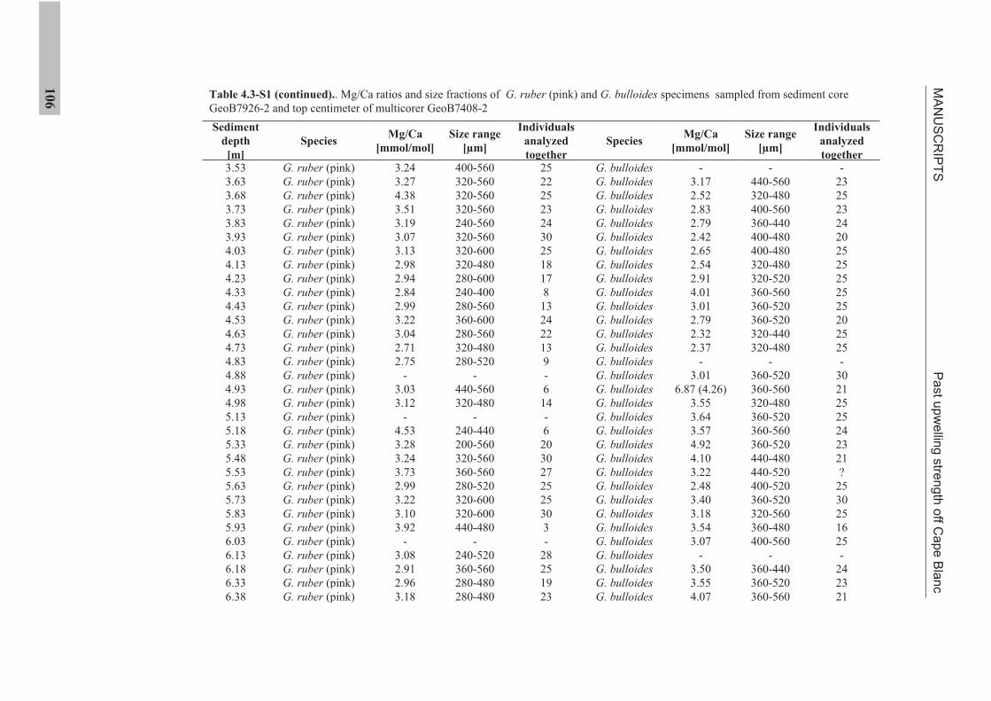
MA
NU
SC
RIP
TS
Pa
st u
pw
ellin
g s
tren
gth
off C
ap
e B
lan
c
106
Individuals
analyzed
together-
23
25
23
24
20
25
25
25
25
25
20
25
25
-
30
21
25
25
24
23
21
?
25
30
25
16
25
-
24
23
21
Size range
[µm]
-
440-560
320-480
400-560
360-440
400-480
400-480
320-480
320-520
360-560
360-520
360-520
320-440
320-480
-
360-520
360-560
320-480
360-520
360-560
360-520
440-480
440-520
400-520
360-520
320-560
360-480
400-560
-
360-440
360-520
360-560
Mg/Ca
[mmol/mol]
-
3.17
2.52
2.83
2.79
2.42
2.65
2.54
2.91
4.01
3.01
2.79
2.32
2.37
-
3.01
6.87 (4.26)
3.55
3.64
3.57
4.92
4.10
3.22
2.48
3.40
3.18
3.54
3.07
-
3.50
3.55
4.07
Species
G. bulloides
G. bulloides
G. bulloides
G. bulloides
G. bulloides
G. bulloides
G. bulloides
G. bulloides
G. bulloides
G. bulloides
G. bulloides
G. bulloides
G. bulloides
G. bulloides
G. bulloides
G. bulloides
G. bulloides
G. bulloides
G. bulloides
G. bulloides
G. bulloides
G. bulloides
G. bulloides
G. bulloides
G. bulloides
G. bulloides
G. bulloides
G. bulloides
G. bulloides
G. bulloides
G. bulloides
G. bulloides
Individuals
analyzed
together25
22
25
23
24
30
25
18
17
8
13
24
22
13
9
-
6
14
-
6
20
30
27
25
25
30
3
-
28
25
19
23
Size range
[µm]
400-560
320-560
320-560
320-560
240-560
320-560
320-600
320-480
280-600
240-400
280-560
360-600
280-560
320-480
280-520
-
440-560
320-480
-
240-440
200-560
320-560
360-560
280-520
320-600
320-600
440-480
-
240-520
360-560
280-480
280-480
Mg/Ca
[mmol/mol]
3.24
3.27
4.38
3.51
3.19
3.07
3.13
2.98
2.94
2.84
2.99
3.22
3.04
2.71
2.75
-
3.03
3.12
-
4.53
3.28
3.24
3.73
2.99
3.22
3.10
3.92
-
3.08
2.91
2.96
3.18
Species
G. ruber (pink)
G. ruber (pink)
G. ruber (pink)
G. ruber (pink)
G. ruber (pink)
G. ruber (pink)
G. ruber (pink)
G. ruber (pink)
G. ruber (pink)
G. ruber (pink)
G. ruber (pink)
G. ruber (pink)
G. ruber (pink)
G. ruber (pink)
G. ruber (pink)
G. ruber (pink)
G. ruber (pink)
G. ruber (pink)
G. ruber (pink)
G. ruber (pink)
G. ruber (pink)
G. ruber (pink)
G. ruber (pink)
G. ruber (pink)
G. ruber (pink)
G. ruber (pink)
G. ruber (pink)
G. ruber (pink)
G. ruber (pink)
G. ruber (pink)
G. ruber (pink)
G. ruber (pink)
Table 4.3-S1 (continued).. Mg/Ca ratios and size fractions of G. ruber (pink) and G. bulloides specimens sampled from sediment core
GeoB7926-2 and top centimeter of multicorer GeoB7408-2
Sediment
depth
[m]3.53
3.63
3.68
3.73
3.83
3.93
4.03
4.13
4.23
4.33
4.43
4.53
4.63
4.73
4.83
4.88
4.93
4.98
5.13
5.18
5.33
5.48
5.53
5.63
5.73
5.83
5.93
6.03
6.13
6.18
6.33
6.38
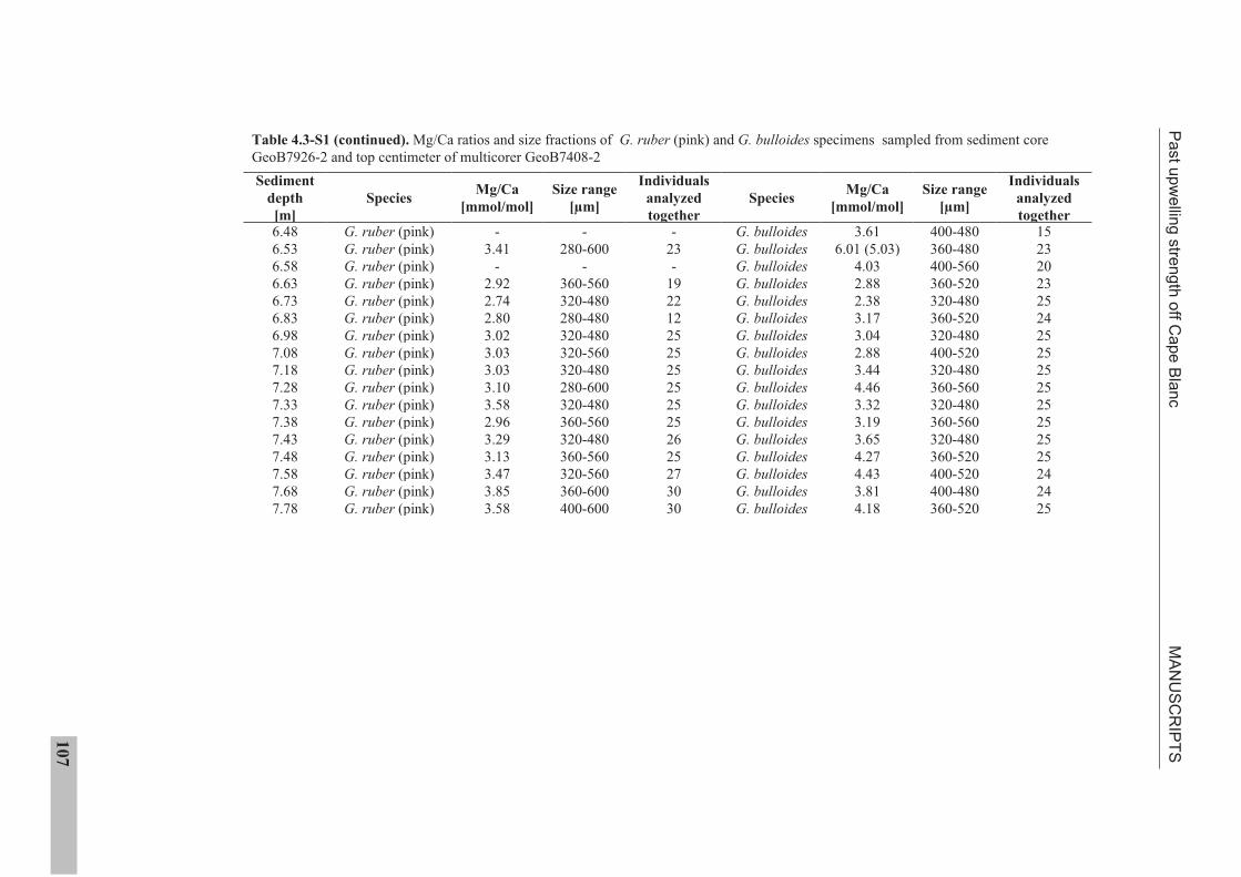
Pa
st u
pw
ellin
g s
tren
gth
off C
ap
e B
lan
c M
AN
US
CR
IPT
S
107
Individuals
analyzed
together15
23
20
23
25
24
25
25
25
25
25
25
25
25
24
24
25
Size range
[µm]
400-480
360-480
400-560
360-520
320-480
360-520
320-480
400-520
320-480
360-560
320-480
360-560
320-480
360-520
400-520
400-480
360-520
Mg/Ca
[mmol/mol]
3.61
6.01 (5.03)
4.03
2.88
2.38
3.17
3.04
2.88
3.44
4.46
3.32
3.19
3.65
4.27
4.43
3.81
4.18
Species
G. bulloides
G. bulloides
G. bulloides
G. bulloides
G. bulloides
G. bulloides
G. bulloides
G. bulloides
G. bulloides
G. bulloides
G. bulloides
G. bulloides
G. bulloides
G. bulloides
G. bulloides
G. bulloides
G. bulloides
Individuals
analyzed
together-
23
-
19
22
12
25
25
25
25
25
25
26
25
27
30
30
Size range
[µm]
-
280-600
-
360-560
320-480
280-480
320-480
320-560
320-480
280-600
320-480
360-560
320-480
360-560
320-560
360-600
400-600
Mg/Ca
[mmol/mol]
-
3.41
-
2.92
2.74
2.80
3.02
3.03
3.03
3.10
3.58
2.96
3.29
3.13
3.47
3.85
3.58
Species
G. ruber (pink)
G. ruber (pink)
G. ruber (pink)
G. ruber (pink)
G. ruber (pink)
G. ruber (pink)
G. ruber (pink)
G. ruber (pink)
G. ruber (pink)
G. ruber (pink)
G. ruber (pink)
G. ruber (pink)
G. ruber (pink)
G. ruber (pink)
G. ruber (pink)
G. ruber (pink)
G. ruber (pink)
Table 4.3-S1 (continued). Mg/Ca ratios and size fractions of G. ruber (pink) and G. bulloides specimens sampled from sediment core
GeoB7926-2 and top centimeter of multicorer GeoB7408-2
Sediment
depth
[m]6.48
6.53
6.58
6.63
6.73
6.83
6.98
7.08
7.18
7.28
7.33
7.38
7.43
7.48
7.58
7.68
7.78

108
SUMMARY AND OUTLOOK
109
V. SUMMARY AND OUTLOOK
5.1 Summary
This thesis investigated the potential of single foraminiferal shells for recording short-
term temperature variations and for reconstructing the water column stratification off NW
Africa in the oceanographic past. Recent studies suggest that interspecimen Mg/Ca and
18Oc differences resemble the seasonal range of temperatures at the sea surface [Sadekov
et al., 2008; Wit et al., 2010]. This was tested for two surface-dwelling species (G. ruber
(white) and G. ruber (pink)) collected in a sediment trap off Cape Blanc. The past water
column stratification at this site was assessed for the past 24,000 years through the
analysis of single specimen 18
Oc of the subsurface-dwelling species G. inflata.
Hypotheses of unexpectedly warm sea surface temperatures (SST) at the study site, due to
decreased upwelling of cold subsurface waters [Romero et al., 2008] were tested, using
the relative abundance of G. bulloides and Mg/Ca analyses of G. ruber (pink),
G. bulloides and G. inflata.
In a sediment trap study (Manuscript I), it was demonstrate that single specimens of
G. ruber (pink) are suitable in the upwelling region off Cape Blanc for tracking the
seasonal amplitude of SST, when the Mg/Ca temperature equation of Regenberg et al.
[2009] is used. Mg/Ca ratios of single G. ruber (white) shells do not track the seasonal
SST and best SST estimates are obtained when using the Elderfield and Ganssen [2000]
Mg/Ca temperature equation. Mg/Ca ratios of G. inflata do not exhibit seasonality and
temperature estimates correspond to calcification depths between the surface and ~400 m
water depth, when using the equation of Elderfield and Ganssen [2000]. The measured
present day variability allowed to calculate that changes in the range between highest and
lowest Mg/Ca ratios are indicative of changes of the calcification temperature range,
when the changes are 0.80 mmol/mol (G. ruber (pink)) or 0.34 mmol/mol (G. inflata).
Single specimens were cleaned prior to analysis using a flow-through system, in order to
prevent sample loss. The previously installed system was further developed during this
PhD project in order to allow for the cleaning of freshly sedimented shells; however the
cleaning of sedimentary shells remains problematic.
For the reconstruction of calcification temperatures from single sedimentary shells, a new
approach recently proposed by Ganssen et al. [2011] was used. In collaboration with the
SUMMARY AND OUTLOOK
110
Section Marine Biogeology at the Vrije Universiteit in Amsterdam (VUA), the
calcification temperature range of single sedimentary G. inflata specimens was
reconstructed for the past 22,000 years by combining conventional Mg/Ca analysis with
single specimen 18
Oc measurements (Manuscript II). It was found that temperature
estimates (12.7 to 17.8°C) agree well with the temperature estimates from the sediment
trap study (11.4 to 20.3°C). Also, the calcification depth range (0-420 m) calculated by
comparison of 18
Oc with 18
Oeq agrees well with the sediment trap study. In order to test
the applicability of single G. inflata specimens for reconstructing past water column
stratification, single specimens from seven time slices between the near present and
22,000 years before present were analyzed from a sediment core retrieved at the same
site. The calcification temperature range was significantly reduced off Cape Blanc during
the last deglaciation as compared to the Last Glacial Maximum and the Holocene.
Comparison to water temperatures predicted by a climate model suggests that the habitat
range of G. inflata was narrower during the last deglaciation as a response to increased
thermal stratification of the water column.
At the study site, previous studies found unexpectedly warm sea surface temperatures,
which were attributed to decreased upwelling strength [Romero et al., 2008]. Upwelling
strength was reconstructed for the past 24,000 years (Manuscript III) and high upwelling
strength found between 24,000 and 16,000 years before present, contradicting this
hypothesis. Mg/Ca temperature reconstructions using the species G. ruber (pink) and
G. bulloides showed a generally high variability throughout the record, in contrast to
Mg/Ca temperatures reconstructed from G. inflata. Inspection of daily SSTs between
1982 and 2008 shows a high degree of local SST variability and substantially increased
local SSTs during years with high wind strength, likely through a northward advection of
warm southerly waters towards the study site. It is presumed that this mechanism might
have also caused high SST variability at the study site in the past.
It was shown in Manuscript I that G. ruber (pink) is likely to record short-term SST
variability. The high variability observed in the downcore G. bulloides record suggests
that this is also true for G. bulloides. This could be tested in future studies by quantifying
the present day Mg/Ca variability between individual specimens of this species collected
from a sediment trap as it was done for G. ruber (pink) in Manuscript I. In the light of
substantial present day SST variability at the study site, it is further desirable to constrain
SUMMARY AND OUTLOOK
111
SST extrema in the past. This could be achieved through analysis of single G. ruber
(pink) and G. bulloides specimens, using combined multispecimen Mg/Ca and single
specimen 18
Oc analysis. More directly the observed variability could be constrained
through Mg/Ca analysis of single shells. This however requires a reliable cleaning of
single sedimentary shells prior to analysis. During this thesis, considerable effort was put
into the further development of the flow-through system, in order to allow for such
cleaning. This work was carried out in collaboration with Dr. Ed C. Hathorne and Dr.
Jeroen Groeneveld and further experiments are still required. Below, the present state of
the art during the time of completion of this thesis is summarized.
5.2 Outlook
Cleaning of sedimentary shells requires a technique that also removes clay contaminants,
which are abundantly found in sedimentary shells and contain 1-10% Mg by weight [Deer
et al., 1992]. These cannot be removed using the previously introduced cleaning
technique. The procedure was therefore modified as follows.
1. As in the previous cleaning, specimens were placed on PTFE filters with a mesh
width of 0.45µm (to hold back clay minerals)
2. Cleaning reagents were applied as listed in Table 5.2-1
3. After cleaning, specimens were kept on the filter and
4. dissolved in a constant flow of acid (mix of 1 M HNO3 pumped at 0.45ml min-1
with suprapure water pumped at 0.1 ml min-1
)
5. The solution was collected in cleaned (soaked for several days in 10% HNO3)
PTFE beakers
6. The solution was then evaporated to a small rest (done by Dr. Ed C. Hathorne in
clean labs of the IFM-GEOMAR, Kiel) which was finally
7. redissolved in 2 ml 0.075 M HNO3 for analysis
For testing this cleaning procedure, single specimens of G. inflata were used, since this
species has a relatively high shell mass (~30µg) that was expected to provide high enough
concentrations in the final solution for Mg/Ca determination on an ICP-OES. The shells
were collected from sediment core GeoB7926-2 at depth intervals (273 and 498 cm), for
which the range of single G. inflata calcification temperatures is well known (conf.
SUMMARY AND OUTLOOK
112
manuscript II). This allowed for excellent control, if the calculated Mg/Ca temperatures
are within a reasonable range.
Element/Ca ratios were determined on a Perkin-Elmer Optima 3300R ICP-OES
equipped with an ultrasonic nebulizer U-5000 AT (Cetac Technologies Inc.) housed at the
faculty of Geosciences, University of Bremen. A solution of international carbonate
reference material ECRM 752-1 was analyzed before and after the samples. Its Mg/Ca
ratio was on average 3.90 mmol/mol (n = 5; = 0.11 mmol/mol), in acceptable agreement
with the reported Mg/Ca ratio of 3.75 mmol/mol [Greaves et al., 2008].
Table 5.2-1. Cleaning program used for cleaning and dissolving single sedimentary foraminifer shells
Duration
[min]
Reagent Pump speed
[ml/min]
Reagent Pump speed
[ml/min]
Destination
Lines below: preconditioning steps for cleaning lines
2 - - 1 M HNO3 3 Waste
3 H2O 3 - - Waste
Lines below: dissolution and collection of single specimens
20 H2O2 4 - - Waste
16.6 H2O 4 - - Waste
2 H2O 0.45 1 M HNO3 0.1 Waste
30 H2O 0.45 1 M HNO3 0.1 Collect
2 H2O 4 - - Waste
The average Al/Ca ratio of 0.40 mmol/mol (n = 5; = 0.05 mmol/mol) was within the
reported Al/Ca ratio of 0.65 (±0.34) mmol/mol and the average Fe/Ca ratio of
0.10 mmol/mol (n = 5; <0.00 mmol/mol) slightly lower than the reported Fe/Ca ratio of
0.17 (±0.03) mmol/mol.
It must be noted that the Al concentrations (on average ~10 ppb) and Fe concentrations
(on average ~5 ppb) were below the calibration range of the ICP-OES for these elements
(40-200 ppb) and should therefore be interpreted with caution and considered an
approximation of the true ratios.
Table 5.2-2 summarizes the results of the analysis and additionally provides Mg/Ca
ratios which are considered realistic, based on the temperature range calculated
previously (conf. manuscript II). As can be seen from Table 5.2-2, the following
difficulties are noted.
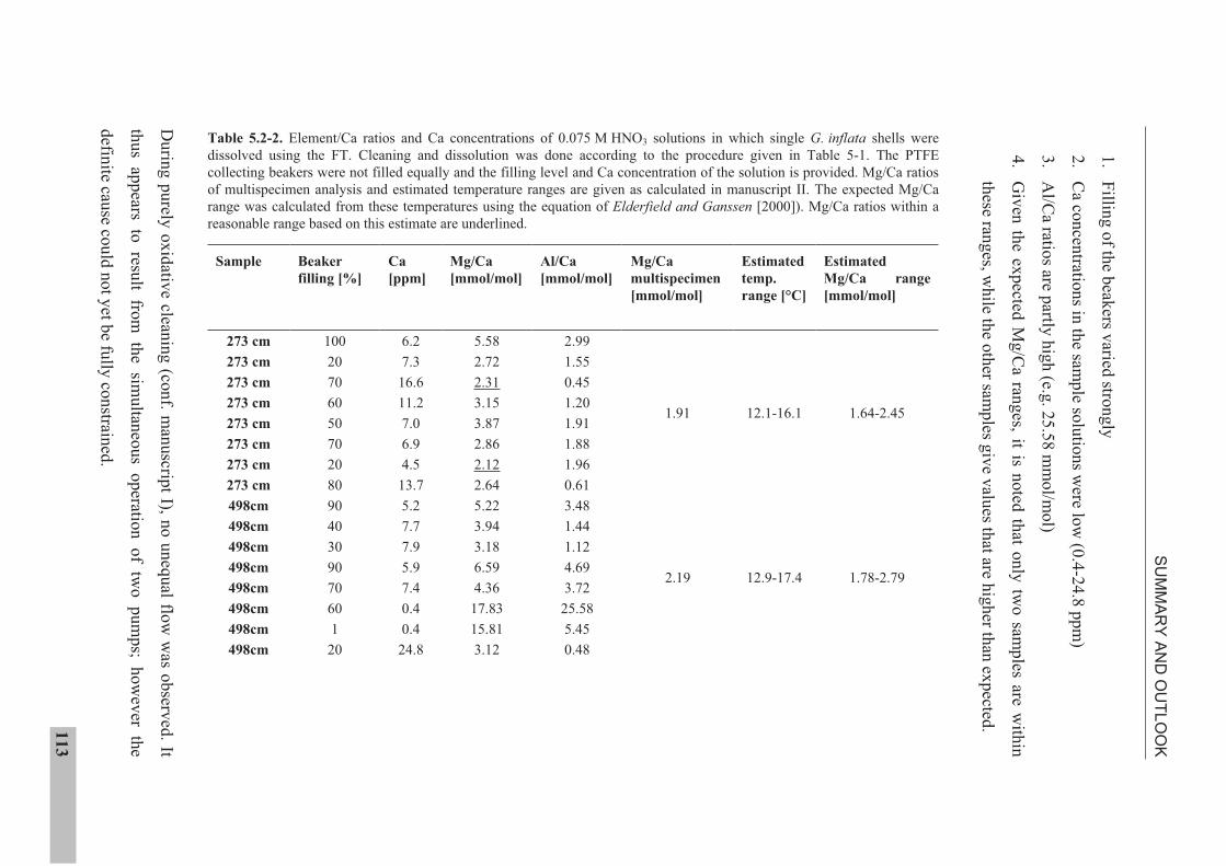
SU
MM
AR
Y A
ND
OU
TL
OO
K
113
1.
Fillin
g o
f the b
eakers v
aried stro
ngly
2.
Ca co
ncen
tration
s in th
e samp
le solu
tion
s were lo
w (0
.4-2
4.8
pp
m)
3.
Al/C
a ratios are p
artly h
igh
(e.g. 2
5.5
8 m
mo
l/mo
l)
4.
Giv
en th
e exp
ected M
g/C
a rang
es, it is no
ted th
at on
ly tw
o sam
ples are w
ithin
these ran
ges, w
hile th
e oth
er samp
les giv
e valu
es that are h
igh
er than
exp
ected.
Estimated
Mg/Ca range
[mmol/mol]
1.64-2.45
1.78-2.79
Estimated
temp.
range [°C]
12.1-16.1
12.9-17.4
Mg/Ca
multispecimen
[mmol/mol]
1.91
2.19
Al/Ca
[mmol/mol]
2.99
1.55
0.45
1.20
1.91
1.88
1.96
0.61
3.48
1.44
1.12
4.69
3.72
25.58
5.45
0.48
Mg/Ca
[mmol/mol]
5.58
2.72
2.31
3.15
3.87
2.86
2.12
2.64
5.22
3.94
3.18
6.59
4.36
17.83
15.81
3.12
Ca
[ppm]
6.2
7.3
16.6
11.2
7.0
6.9
4.5
13.7
5.2
7.7
7.9
5.9
7.4
0.4
0.4
24.8
Beaker
filling [%]
100
20
70
60
50
70
20
80
90
40
30
90
70
60
1
20
Table 5.2-2. Element/Ca ratios and Ca concentrations of 0.075 M HNO3 solutions in which single G. inflata shells were
dissolved using the FT. Cleaning and dissolution was done according to the procedure given in Table 5-1. The PTFE
collecting beakers were not filled equally and the filling level and Ca concentration of the solution is provided. Mg/Ca ratios
of multispecimen analysis and estimated temperature ranges are given as calculated in manuscript II. The expected Mg/Ca
range was calculated from these temperatures using the equation of Elderfield and Ganssen [2000]). Mg/Ca ratios within a
reasonable range based on this estimate are underlined.
Sample
273 cm
273 cm
273 cm
273 cm
273 cm
273 cm
273 cm
273 cm
498cm
498cm
498cm
498cm
498cm
498cm
498cm
498cm
Durin
g p
urely
ox
idativ
e cleanin
g (co
nf. m
anuscrip
t I), no u
neq
ual flo
w w
as observ
ed. It
thu
s ap
pears
to
result
from
th
e sim
ultan
eou
s o
peratio
n
of
two
p
um
ps;
ho
wev
er th
e
defin
ite cause co
uld
no
t yet b
e fully
con
strained
.
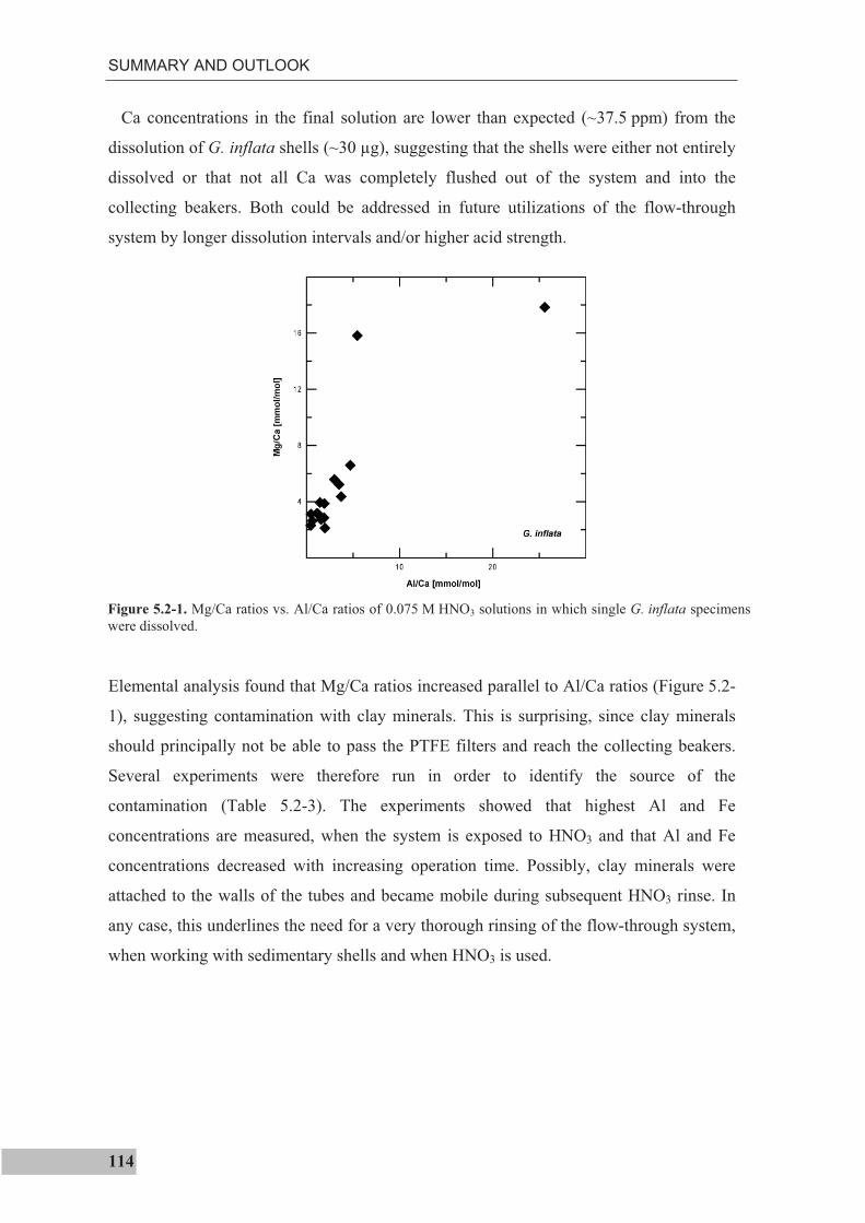
SUMMARY AND OUTLOOK
114
Ca concentrations in the final solution are lower than expected (~37.5 ppm) from the
dissolution of G. inflata shells (~30 µg), suggesting that the shells were either not entirely
dissolved or that not all Ca was completely flushed out of the system and into the
collecting beakers. Both could be addressed in future utilizations of the flow-through
system by longer dissolution intervals and/or higher acid strength.
Elemental analysis found that Mg/Ca ratios increased parallel to Al/Ca ratios (Figure 5.2-
1), suggesting contamination with clay minerals. This is surprising, since clay minerals
should principally not be able to pass the PTFE filters and reach the collecting beakers.
Several experiments were therefore run in order to identify the source of the
contamination (Table 5.2-3). The experiments showed that highest Al and Fe
concentrations are measured, when the system is exposed to HNO3 and that Al and Fe
concentrations decreased with increasing operation time. Possibly, clay minerals were
attached to the walls of the tubes and became mobile during subsequent HNO3 rinse. In
any case, this underlines the need for a very thorough rinsing of the flow-through system,
when working with sedimentary shells and when HNO3 is used.
Figure 5.2-1. Mg/Ca ratios vs. Al/Ca ratios of 0.075 M HNO3 solutions in which single G. inflata specimens
were dissolved.
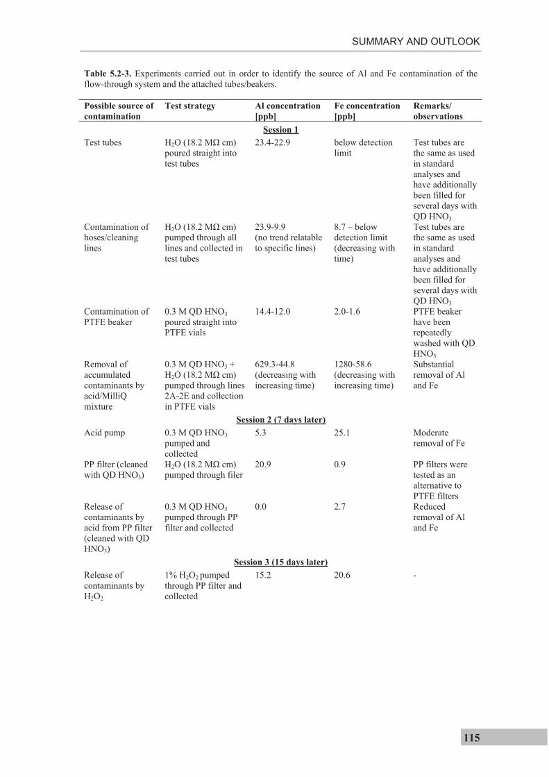
SUMMARY AND OUTLOOK
115
Table 5.2-3. Experiments carried out in order to identify the source of Al and Fe contamination of the
flow-through system and the attached tubes/beakers.
Possible source of
contamination
Test strategy Al concentration
[ppb]
Fe concentration
[ppb]
Remarks/
observations
Session 1
Test tubes H2O (18.2 M cm)
poured straight into
test tubes
23.4-22.9 below detection
limit
Test tubes are
the same as used
in standard
analyses and
have additionally
been filled for
several days with
QD HNO3
Contamination of
hoses/cleaning
lines
H2O (18.2 M cm)
pumped through all
lines and collected in
test tubes
23.9-9.9
(no trend relatable
to specific lines)
8.7 – below
detection limit
(decreasing with
time)
Test tubes are
the same as used
in standard
analyses and
have additionally
been filled for
several days with
QD HNO3
Contamination of
PTFE beaker
0.3 M QD HNO3
poured straight into
PTFE vials
14.4-12.0 2.0-1.6 PTFE beaker
have been
repeatedly
washed with QD
HNO3
Removal of
accumulated
contaminants by
acid/MilliQ
mixture
0.3 M QD HNO3 +
H2O (18.2 M cm)
pumped through lines
2A-2E and collection
in PTFE vials
629.3-44.8
(decreasing with
increasing time)
1280-58.6
(decreasing with
increasing time)
Substantial
removal of Al
and Fe
Session 2 (7 days later)
Acid pump 0.3 M QD HNO3
pumped and
collected
5.3 25.1 Moderate
removal of Fe
PP filter (cleaned
with QD HNO3)
H2O (18.2 M cm)
pumped through filer
20.9 0.9 PP filters were
tested as an
alternative to
PTFE filters
Release of
contaminants by
acid from PP filter
(cleaned with QD
HNO3)
0.3 M QD HNO3
pumped through PP
filter and collected
0.0 2.7 Reduced
removal of Al
and Fe
Session 3 (15 days later)
Release of
contaminants by
H2O2
1% H2O2 pumped
through PP filter and
collected
15.2 20.6 -

116

REFERENCES
117
VI. REFERENCES
Abrantes, F. (2000), 200,000 yr diatom records from Atlantic upwelling sites reveal
maximum productivity during LGM and a shift in phytoplankton community structure at
185,000 yr, Earth Planet. Sc. Lett., 176(1), 7-16.
Adkins, J., P. deMenocal, and G. Eshel (2006), The "African humid period" and the
record of marine upwelling from excess 230Th in Ocean Drilling Program Hole 658C,
Paleoceanography, 21(4), PA4203.
Anand, P., and H. Elderfield (2005), Variability of Mg/Ca and Sr/Ca between and within
the planktonic foraminifers Globigerina bulloides and Globorotalia truncatulinoides,
Geochem. Geophys. Geosyst., 6(11), Q11D15.
Anand, P., H. Elderfield, and M. H. Conte (2003), Calibration of Mg/Ca thermometry in
planktonic foraminifera from a sediment trap time series, Paleoceanography, 18(2), 1050.
Antonov, J. I., R. A. Locarnini, T. P. Boyer, A. V. Mishonov, and H. E. Garcia (2006),
World Ocean Atlas 2005, Volume 2: Salinity, in NOAA Atlas NESDIS 62, edited by S.
Levitus, U.S. Government Printing Office, Washinton D.C., 182 pp.
Arbuszewski, J., P. deMenocal, A. Kaplan, and E. C. Farmer (2010), On the fidelity of
shell-derived18
Oseawater estimates, Earth and Planetary Science Letters, 300 (3-4),
185-196.
Arhan, M., A. Colin De Verdiére, and L. Mémery (1994), The Eastern Boundary of the
Subtropical North Atlantic, Journal of Physical Oceanography, 24(6), 1295-1316.
Bakun, A. (1990), Global Climate Change and Intensification of Coastal Ocean
Upwelling, Science, 247(4939), 198-201.
Barker, S., M. Greaves, and H. Elderfield (2003), A study of cleaning procedures used for
foraminiferal Mg/Ca paleothermometry, Geochem. Geophys. Geosyst., 4.
Barton, E. D. (2001), Canary and Portugal Currents, University of Wales Academic Press.
Bé, A. W. H. (1960), Ecology of recent planktonic foraminifera: Part 2 - Bathymetric and
seasonal distribution in the Sargasso Sea off Bermuda, Micropaleontology, 6, 373-392.
Bé, A. W. H., and W. H. Hamlin (1967), Ecology of Recent Planktonic Foraminifera: Part
3: Distribution in the North Atlantic during the Summer of 1962, Micropaleontology,
13(1), 87-106.
Bé, A. W. H. (1977), An ecological, zoogeographic and taxonomic review of recent
planktonic foraminifera, in Oceanic Micropaleontology, edited by A. T. S. Ramsay,
Academic Press, London, pp. 1-100
Bé, A. W. H., and H. J. Spero (1981), Shell regeneration and biological recovery of
planktonic foraminifera after physical injury induced in laboratory culture,
Micropaleontology, 27(3), 305-316.
REFERENCES
118
Bemis, B. E., H. J. Spero, J. Bijma, and D. W. Lea (1998), Reevaluation of the oxygen
isotopic composition of planktonic foraminifera: Experimental results and revised
paleotemperature equations, Paleoceanography, 13(2), 150-160.
Benway, H. M., B. A. Haley, G. P. Klinkhammer, and A. C. Mix (2003), Adaptation of a
flow-through leaching procedure for Mg/Ca paleothermometry, Geochem. Geophys.
Geosyst., 4.
Bijma, J., J. Erez, and C. Hemleben (1990), Lunar and semi-lunar reproductive-cycles in
some spinose planktonic foraminifers, Journal of Foraminiferal Research, 20(2), 117-
127.
Billups, K., and H. J. Spero (1996), Reconstructing the stable isotope geochemistry and
paleotemperatures of the equatorial Atlantic during the last 150,000 years: Results from
individual foraminifera, Paleoceanography, 11(2), 217-238.
Boyle, E. A. (1981), Cadmium, zinc, copper, and barium in foraminifera tests, Earth
Planet. Sc. Lett., 53(1), 11-35.
Caron, D. A., O. Roger Anderson, J. L. Lindsey, J. W. W. Faber, and E. E. Lin Lim
(1990), Effects of gametogenesis on test structure and dissolution of some spinose
planktonic foraminifera and implications for test preservation, Mar. Micropaleontol.,
16(1-2), 93-116.
Chapman, M. R., N. J. Shackleton, M. Zhao, and G. Eglinton (1996), Faunal and
alkenone reconstructions of subtropical North Atlantic surface hydrography and
paleotemperature over the last 28 kyr, Paleoceanography, 11(3), 343-357.
Chiessi, C. M., S. Ulrich, S. Mulitza, J. Pätzold, and G. Wefer (2007), Signature of the
Brazil-Malvinas Confluence (Argentine Basin) in the isotopic composition of planktonic
foraminifera from surface sediments, Mar. Micropaleontol., 64(1-2), 52-66.
Clarke, F. W., and W. C. Wheeler (1922), The inorganic constituents of marine
invertebrates, USGS Prof. Pap., 124, 55.
Cléroux, C., E. Cortijo, J.-C. Duplessy, and R. Zahn (2007), Deep-dwelling foraminifera
as thermocline temperature recorders, Geochem. Geophys. Geosyst., 8.
Cléroux, C., E. Cortijo, P. Anand, L. Labeyrie, F. Bassinot, N. Caillon, and J.-C.
Duplessy (2008), Mg/Ca and Sr/Ca ratios in planktonic foraminifera: Proxies for upper
water column temperature reconstruction, Paleoceanography, 23, PA3214.
Curry, W. B., R. C. Thunell, and S. Honjo (1983), Seasonal changes in the isotopic
composition of planktonic foraminifera collected in Panama Basin sediment traps, Earth
and Planetary Science Letters, 64(1), 33-43.
Davis, K. J., P. M. Dove, and J. J. De Yoreo (2000), The Role of Mg2+ as an Impurity in
Calcite Growth, Science, 290, 1134-1137.
REFERENCES
119
Dekens, P. S., D. W. Lea, D. K. Pak, and H. J. Spero (2002), Core top calibration of
Mg/Ca in tropical foraminifera: Refining paleotemperature estimation, Geochem.
Geophys. Geosyst., 3(4).
Dekens, P. S., A. C. Ravelo, M. D. McCarthy, and C. A. Edwards (2008), A 5 million
year comparison of Mg/Ca and alkenone paleothermometers, Geochem. Geophys.
Geosyst., 9.
Deer, W. A., R. A. Howie, and J. Zussman (1992), An introduction to the Rock Forming
Minerals (second edition), Longman Reading, Mass.; 712 pp.
Deuser, W. G., E. H. Ross, C. Hemleben, and M. Spindler (1981), Seasonal changes in
species composition, numbers, mass, size, and isotopic composition of planktonic
foraminifera settling into the deep sargasso sea, Palaeogeography, Palaeoclimatology,
Palaeoecology, 33(1–3), 103-127.
Diester-Haass, L. (1973), Absolute abundance pf particles and planktic foraminifera in
sediment core GIK12301-4, Cape Barbas, North-West Africa, PANGAEA data repository.
Elderfield, H., and G. Ganssen (2000), Past temperature and delta-18
O of surface ocean
waters inferred from foraminiferal Mg/Ca ratios, Nature, 18, 442-445.
Elderfield, H., M. Vautravers, and M. Cooper (2002), The relationship between shell size
and Mg/Ca, Sr/Ca, 18
O, and 13
C of species of planktonic foraminifera, Geochem.
Geophys. Geosyst., 3.
Emiliani, C. (1955), Pleistocene Temperatures, The Journal of Geology, 63(6), 538-578.
Erez, J., and S. Honjo (1981), Comparison of isotopic composition of planktonic
foraminifera in plankton tows, sediment traps and sediments, Palaeogeogr. Palaeocl.,
33(1-3), 129-156.
Fairbanks, R. G., P. H. Wiebe, and A. W. H. Be (1980), Vertical Distribution and Isotopic
Composition of Living Planktonic Foraminifera in the Western North Atlantic, Science,
207, 61-63.
Fairbanks, R. G., M. Sverdlove, R. Free, P. H. Wiebe, and A. W. H. Be (1982), Vertical
distribution and isotopic fractionation of living planktonic foraminifera from the Panama
Basin, Nature, 298, 841-844.
Farmer, E. C., A. Kaplan, P. B. de Menocal, and J. Lynch-Stieglitz (2007), Corroborating
ecological depth preferences of planktonic foraminifera in the tropical Atlantic with the
stable oxygen isotope ratios of core top specimens, Paleoceanography, 22(3), PA3205.
Farmer, E. J., M. R. Chapman, and J. E. Andrews (2010), North Atlantic Globorotalia
inflata coretop Mg/Ca calibrations and temperature reconstructions over Termination I,
IOP Conf. Ser.: Earth Environ. Sci., 9, 1-7.
Ferguson, J. E., G. M. Henderson, M. Kucera, and R. E. M. Rickaby (2008), Systematic
change of foraminiferal Mg/Ca ratios across a strong salinity gradient, Earth and
Planetary Science Letters, 265(1-2), 153-166.
REFERENCES
120
Filipsson, H. L., O. E. Romero, J.-B. W. Stuut, and B. Donner (2011), Relationships
between primary productivity and bottom-water oxygenation off northwest Africa during
the last deglaciation, Journal of Quaternary Science, 26(4), 448-456.
Fischer, G., B. Donner, V. Ratmeyer, R. Davenport, and G. Wefer (1996), Distinct year-
to-year particle flux variations off Cape Blanc during 1988-1991: Relation to 18
O-
deduced sea-surface temperatures and trade winds, Journal of Marine Research, 54(1),
73-98.
Fischer, G., G. Ruhland, and cruise participants (2008), Report and preliminary results of
Poseidon cruise 344, Leg 1 & Leg 2, Las Palmas -Las Palmas, Berichte, Fachbereich
Geowissenschaften, 259, 47.
Freudenthal, T., H. Meggers, J. Henderiks, H. Kuhlmann, A. Moreno, and G. Wefer
(2002), Upwelling intensity and filament activity off Morocco during the last 250,000
years, Deep Sea Research Part II: Topical Studies in Oceanography, 49(17), 3655-3674.
Gabric, A. J., L. Garcia, L. Van Camp, L. Nykjaer, W. Eifler, and W. Schrimpf (1993),
Offshore export of shelf production in the Cape Blanc (Mauritania) giant filament as
derived from coastal zone color scanner imagery, J. Geophys. Res., 98, 4697-4712.
Ganssen, G., and M. Sarnthein (1983), Stable-isotope composition of foraminifers: the
surface and bottom water record of coastal upwelling, in Coastal Upwelling: Its
Sedimentary Record, edited by J. Thiede and E. Suess, Plenum, New York, pp. 99-121.
Ganssen, G. M., and D. Kroon (2000), The isotopic signature of planktonic foraminifera
from NE Atlantic surface sediments: implications for the reconstruction of past oceanic
conditions, J. Geol. Soc. London, 157(3), 693-699.
Ganssen, G. M., F. J. C. Peeters, B. Metcalfe, P. Anand, S. J. A. Jung, D. Kroon, and G. J.
A. Brummer (2011), Quantifying sea surface temperature ranges of the Arabian Sea for
the past 20 000 years, Clim. Past, 7(4), 1337-1349.
Gastrich, M. D. (1987), Ultrastructure of a new intracellular symbiotic alga found within
planktonic foraminfera, J. Phycol., 23, 623-632.
Greaves, M., et al. (2008), Interlaboratory comparison study of calibration standards for
foraminiferal Mg/Ca thermometry, Geochem. Geophys. Geosyst., 9(8), Q08010.
Groeneveld, J., and C. M. Chiessi (2011), Mg/Ca of Globorotalia inflata as a recorder of
permanent thermocline temperatures in the South Atlantic, Paleoceanography, 26(2),
PA2203.
Haarmann, T., E. Hathorne, M. Mohtadi, J. Groeneveld, M. Kölling, and T. Bickert
(2011), Mg/Ca ratios of single planktonic foraminifer shells and the potential to
reconstruct the thermal seasonality of the water column, Paleoceanography, 26, PA3218.
Hagen, E., and R. Schemainda (1987), On the annual distribution of South Atlantic
Central Water (SACW) along a section off Cape Blanc, Northwest Africa, Oceanol. Acta,
19, 61-70.
REFERENCES
121
Hagen, E. (2001), Northwest African upwelling scenario, Oceanol. Acta, 24 (Suppl. 1),
113-128.
Haley, B. A., and G. P. Klinkhammer (2002), Development of a flow-trough system for
cleaning and dissolving foraminiferal tests, Chem. Geol., 185, 51-69.
Hammer, Ø., D. A. T. Harper, and P. D. Ryan (2001), PAST: Paleontological Statistics
software package for education and data analysis, Palaeontologia Electronica, 4(1), 9.
Haslett, S. K., and C. W. Smart (2006), Late Quaternary upwelling off NW Africa: new
micropaleontological evidence from ODP hole 658C, J. Quaternary Sci., 21(3), 259-269.
Hastings, D. W., S. R. Emerson, J. Erez, and B. K. Nelson (1996), Vanadium in
foraminiferal calcite: Evaluation of a method to determine paleo-seawater vanadium
concentrations, Geochim. Cosmochim. Ac., 60(19), 3701-3715.
Hathorne, E. C., R. H. James, and R. S. Lampitt (2009), Environmental versus
biomineralization controls on the intratest variation in the trace element composition of
the planktonic foraminifera G. inflata and G. scitula, Paleoceanography, 24, PA4204.
Hecht, M. W., and H. H. Hasumi (Eds.) (2008), Ocean Modeling in an Eddying Regime,
Geophys. Monogr. Ser. (vol. 177), AGU, Washington, D.C.
Helmke, P., O. Romero, and G. Fischer (2005), Northwest African upwelling and its
effect on offshore organic carbon export to the deep sea, Global Biogeochem. Cycles,
19(4), GB4015.
Hemleben, C., M. Spindler, and O. R. Anderson (1989), Modern Planktonic
Foraminifera, Springer-Verlag, New York, 363 pp.
Henderiks, J., T. Freudenthal, H. Meggers, and S. Nave (2002), Glacial-interglacial
variability of particle accumulation in the Canary Basin: a time-slice approach, Deep Sea
Research II, 49, 3675-3705.
Huang, E., S. Mulitza, A. Paul, J. Groeneveld, S. Steinke, and M. Schulz (submitted),
Response of the eastern tropical Atlantic central waters to thermohaline circulation
changes during the Last Glacial Maximum and Heinrich Stadial 1.
Khider, D., L. D. Stott, J. Emile-Geay, R. Thunell, and D. E. Hammond (2011), Assessing
El Niño Southern Oscillation variability during the past millennium, Paleoceanography,
26(3), PA3222.
Killingley, J. S., R. F. Johnson, and W. H. Berger (1981), Oxygen and carbon isotopes of
individual shells of planktonic foraminifera from Ontong-Java plateau, equatorial pacific,
Palaeogeography, Palaeoclimatology, Palaeoecology, 33(1-3), 193-204.
Kim, S.-T., and J. R. O'Neil (1997), Equilibrium and nonequilibrium oxygen isotope
effects in synthetic carbonates, Geochim. Cosmochim. Ac., 61(16), 3461-3475.
REFERENCES
122
King, A. L., and W. R. Howard (2005), 18O seasonality of planktonic foraminifera from
Southern Ocean sediment traps: Latitudinal gradients and implications for paleoclimate
reconstructions, Mar. Micropaleontol., 56(1-2), 1-24.
Kisakürek, B. A., A. Eisenhauer, F. Böhm, D. Garbe-Schönberg, and J. Erez (2008),
Controls on shell Mg/Ca and Sr/Ca in cultured planktonic foraminiferan, Globigerinoides
ruber (white), Earth Planet. Sc. Lett., 273(3-4), 260-269.
Koutavas, A., P. B. deMenocal, G. C. Olive, and J. Stieglitz-Lynch (2006), Mid-Holocene
El Niño-Southern Oscillation (ENSO) attentuation revealed by individual foraminifera in
eastern tropical Pacific sediments, Geology, 34(12), 993-996.
Ku era, M. (2007), Planktonic foraminifera as tracers of past oceanic environments, in
Proxies in Late Cenozoic Paleoceanography, edited by Hillaire-Marcel, C. and de Vernal,
A., Developments in Marine Geology (vol.1), Elsevier, Amsterdam, pp. 213-262
Kuhlmann, H., T. Freudenthal, P. Helmke, and H. Meggers (2004), Reconstruction of
paleoceanography off NW Africa during the last 40,000 years: influence of local and
regional factors on sediment accumulation, Marine Geology, 207(1-4), 209-224.
Lachkar, Z., and N. Gruber (2011), What controls biological production in coastal
upwelling systems? Insights from a comparative modeling study, Biogeosciences, 8(10),
2961-2976.
Lea, D. W., and E. A. Boyle (1991), Barium in planktonic foraminifera, Geochim.
Cosmochim. Ac., 55(11), 3321-3331.
Lea, D. W., T. A. Mashiotta, and H. J. Spero (1999), Controls on magnesium and
strontium uptake in planktonic foraminifera determined by live culturing, Geochimica et
Cosmochimica Acta, 63(16), 2369-2379.
Lea, D. W., D. K. Pak, and H. J. Spero (2000), Climate impact of Late Quaternary
Equatorial Pacific sea surface temperature variations, Science, 289, 1719-1724.
Leduc, G., L. Vidal, O. Cartapanis, and E. Bard (2009), Modes of eastern equatorial
Pacific thermocline variability: Implications for ENSO dynamics over the last glacial
period, Paleoceanography, 24.
Liu, Z., et al. (2009), Transient Simulation of Last Deglaciation with a New Mechanism
for Bølling-Allerød Warming, Science, 325(5938), 310-314.
Locarnini, R. A., A. V. Mishonov, J. I. Antonov, T. P. Boyer, and H. E. Garcia (2006),
World Ocean Atlas 2005, Volume 1: Temperature, in NOAA Atlas NESDIS 61, edited by
S. Levitus, p. 182, U.S. Government Printing Office, Washington, D.C.
Lohmann, G. P. (1995), A model for variation in the chemistry of planktonic foraminifera
due to secondary calcification and selective dissolution, Paleoceanography, 10(3), 445-
457.
REFERENCES
123
Lon ari , N., F. J. C. Peeters, D. Kroon, and G.-J. A. Brummer (2006), Oxygen isotope
ecology of recent planktic foraminifera at the central Walvis Ridge (SE Atlantic),
Paleoceanography, 21(3), PA3009.
Marr, J. P., J. A. Baker, L. Carter, A. S. R. Allan, G. B. Dunbar, and H. C. Bostock
(2011), Ecological and temperature controls on Mg/Ca ratios of Globigerina bulloides
from the southwest Pacific Ocean, Paleoceanography, 26(2), PA2209.
Martinez, P., P. Bertrand, G. B. Shimmield, C. Karen, F. J. Jorissen, J. Foster, and M.
Dignan (1999), Upwelling intensity and ocean productivity changes off Cape Blanc
(northwest Africa) during the last 70,000 years: geochemical and micropalaeontological
evidence, Marine Geology, 158(1-4), 57-74.
Merkel, U., M. Prange, and M. Schulz (2010), ENSO variability and teleconnections
during glacial climates, Quaternary Science Reviews, 29(1-2), 86-100.
Meggers, H., M. Bergenthal, and C. participants (2002), Report of R/V Poseidon cruise
POS 272, Las Palmas-Las Palmas, 1.4.-14.4.2001, Berichte, Fachbereich
Geowissenschaften, 197, 19.
Meggers, H., and cruise participants (2003), Report and preliminary results of METEOR
Cruise M53/1, Limassol - Las Palmas - Mindelo, 30.03.2002 - 03.05.2002, Berichte,
Fachbereich Geowissenschaften, Universität Bremen, 214, 81.
McConnell, M. C., and R. C. Thunell (2005), Calibration of the planktonic foraminiferal
Mg/Ca paleothermometer: Sediment trap results from the Guaymas Basin, Gulf of
California, Paleoceanography, 20, PA2016.
McKenna, V. S., and W. L. Prell (2004), Calibration of the Mg/Ca of Globorotalia
truncatulinoides (R) for the reconstruction of marine temperature gradients,
Paleoceanography, 19(2), PA2006.
Mittelstaedt, E. (1983), The upwelling area off Northwest Africa - A description of
phenomena related to coastal upwelling, Progress In Oceanography, 12(3), 307-331.
Mohtadi, M., S. Steinke, J. Groeneveld, H. G. Fink, T. Rixen, D. Hebbeln, B. Donner, and
B. Herunadi (2009), Low-latitude control on seasonal and interannual changes in
planktonic foraminiferal flux and shell geochemistry off south Java: A sediment trap
study, Paleoceanography, 24., PA1201.
Mulitza, S., W. Dürkoop, W. Hale, and G. Wefer (1997), Planktonic foraminifera as
recorders of past surface-water stratification, Geology, 24(4), 335-338.
Mulitza, S., T. Wolff, J. Pätzold, W. Hale, and G. Wefer (1998), Temperature sensitivity
of planktonic foraminifera and its influence on the oxygen isotope record, Mar.
Micropaleontol., 33, 223-240.
Mulitza, S., B. Donner, G. Fischer, A. Paul, J. Pätzold, C. Rühlemann, and M. Segel
(2004), The South Atlantic oxygen isotope record of planktic foraminifera, in The South
Atlantic in the Late Quarternary: Reconstruction of Material Budgets and Current Systems, edited by G. Wefer, S. Mulitza and V. Ratmeyer, Springer, Berlin, pp. 121-142.
REFERENCES
124
Narayan, N., A. Paul, S. Mulitza, and M. Schulz (2010), Trends in coastal upwelling
insensity during the late 20th century, Ocean Science, 6, 815-823.
Nürnberg, D., J. Bijma, and C. Hemleben (1996), Assessing the reliability of magnesium
in foraminiferal calcite as a proxy for water mass temperatures, Geochim. Cosmochim.
Ac., 60(5), 803-814.
Nykjær, L., and L. Van Camp (1994), Seasonal and interannual variability of coastal
upwelling along northwest Africa and Portugal from 1981 to 1991, J. Geophys. Res.,
99(C7), 14197-14207.
Okai, T., A. Suzuki, S. Terashima, M. Inoue, M. Nohara, H. Kawahata, and N. Imai
(2004), Collaborative analysis of GSJ/AIST geochemical reference materials JCp-1
(Coral) and JCt-1 (Giant Clam), Chikyukagaku, 38, 281-286.
Pastor, M. V., J. L. Pelegrí, A. Hernández-Guerra, J. Font, J. Salat, and M. Emelianov
(2008), Water and nutrient fluxes off Northwest Africa, Continental Shelf Research,
28(7), 915-936.
Pelegrí, J. L., J. Arístegui, L. Cana, M. González-Dávila, and A. Hernández-Guerra
(2005), Coupling between the open ocean and the coastal upwelling region off northwest
Africa: water recirculation and offshore pumping of organic matter, J. Marine Syst., 54,
3-37.
Pérez-Rodríguez, P., J. L. Pelegrí, and A. Marrero-Díaz (2001), Dynamical characteristics
of the Cape Verde frontal zone, Sci. Mar., 65, 241-250.
Pierre, C., A. Vangriesheim, and E. Laube-Lenfant (1994), Variability of water masses
and of organic production-regeneration systems as related to eutrophic, mesotropic and
oligotrophic conditions in the northeast Atlantic Ocean, J. Marine Syst., 5(2), 159-170.
Reimer, P. J., et al. (2009), IntCal09 and Marine09 radiocarbon age calibration curves, 0 –
50,000 years cal BP, Radiocarbon, 51(4), 1111-1150.
Rashid, H., and E. A. Boyle (2007), Mixed-Layer Deepening During Heinrich Events: A
Multi-Planktonic Foraminiferal 18
O Approach, Science, 318(5849), 439-441.
Ravelo, A. C., R. G. Fairbanks, and S. G. H. Philander (1990), Reconstructing tropical
Atlantic hydrography using planktonic foraminifera and an ocean model,
Paleoceanography, 5, 409-431.
Regenberg, M., S. Steph, D. Nürnberg, R. Tiedemann, and D. Garbe-Schönberg (2009),
Calibrating Mg/Ca ratios of multiple planktonic foraminiferal species with 18
O-
calcification temperatures: Paleothermometry for the upper water column, Earth Planet.
Sc. Lett., 278(3-4), 324-336.
Romero, O. E., J.-H. Kim, and B. Donner (2008), Submillennial-to-millennial variability
of diatom production off Mauritania, NW Africa, during the last glacial cycle,
Paleoceanography, 23, PA3218.
REFERENCES
125
Rosenthal, Y., M. P. Field, and R. M. Sherrell (1999), Precise determination of
element/calcium ratios in calcareous samples using sector field inductively coupled
plasma mass spectrometry, Analytical Chemistry, 71(15), 3248-3253.
Russell, A. D., and H. J. Spero (2000), Field Examination of the Oceanic Carbonate Ion
Effect on Stable Isotopes in Planktonic Foraminifera, Paleoceanography, 15(1), 43-52.
Sadekov, A., S. M. Eggins, P. De Deckker, and D. Kroon (2008), Uncertainties in
seawater thermometry deriving from intratest and intertest Mg/Ca variability in
Globigerinoides ruber, Paleoceanography, 23(1), PA1215.
Sautter, L. R., and R. C. Thunell (1991), Seasonal Variability in the 18
O and 13
C of
Planktonic Foraminifera from an Upwelling Environment: Sediment Trap Results from
the San Pedro Basin, Southern California Bight, Paleoceanography, 6(3), 307-334.
Sautter, L. R., and C. Sancetta (1992), Seasonal associations of phytoplankton and
planktic foraminifera in an upwelling region and their contribution to the seafloor, Marine
Micropaleontology, 18(4), 263-278.
Schemainda, R., P. Nehring, and S. Schulz (1975), Ozeanologische Untersuchungen zum
Produktionspotential der nordwestafrikanischen Wasserauftriebsregion, Nationalkomitee
für Geodäsie und Geophysik bei der Akademie der Wissenschaften der Deutschen
Demokratischen Republik, Berlin 88 pp.
Schmidt, G. A., G. R. Bigg, and E. J. Rohling (1999), Global Seawater Oxygen-18
Database, http://data.giss.nasa.gov/o18data/.
Shackleton, N. J. (1967), Oxygen isotopic analyses and Pleistocene temperatures re-
assessed, Nature, 215, 15-17.
Shackleton, N. J. (1974), Attainment of isotopic equilibrium between ocean water and the
benthonic foraminifera genus Uvigerina: isotopic changes in the ocean during the last
glacial, Cent. Nat. Rech. Sci. Colloq. Int., 219, 203-209.
Shapiro, S. S., and M. B. Wilk (1965), An analysis of variance test for normality
(complete samples), Biometrika, 52, 591-611.
She, J., J. L. Høyer, and J. Larsen (2007), Assessment of sea surface temperature
observational networks in the Baltic Sea and North Sea, J. Marine Syst., 65(1-4), 314-
335.
Siegel, D. A., T. C. Granata, A. F. Michaels, and T. D. Dickey (1990), Mesoscale eddy
diffusion, particle sinking, and the interpretation of sediment trap data, J. Geophys. Res.,95(C4), 5305-5311.
Sicre, M.-A., Y. Ternois, M. Paterne, P. Martinez, and P. Bertrand (2001), Climatic
changes in the upwelling region off Cap Blanc, NW Africa, over the last 70 kyear: a
multi-biomarker approach, Organic Geochemistry, 32(8), 981-990.
REFERENCES
126
Spero, H. J., and D. F. Williams (1990), Evidence for Seasonal Low-Salinity Surface
Waters in the Gulf of Mexico Over the Last 16,000 Years, Paleoceanography, 5(6), 963-
975.
Speth, P., H. Detlefsen, and H.-W. Sierts (1978), Meteorological influences on upwelling
off Northwest Africa, Dt. Hydrogr. Z., 31(3), 98-104.
Spindler, M., C. Hemleben, U. Bayer, A. W. H. Bé, and O. R. Anderson (1979), Lunar
periodicity of reproduction in the planktonic foraminifer Hastigerina pelagica, Marine
Ecology Progress Series, 1, 61-64.
Steph, S., M. Regenberg, R. Tiedemann, S. Mulitza, and D. Nürnberg (2009), Stable
isotopes of planktonic foraminifera from tropical Atlantic/Caribbean coretops:
Implications for reconstructing upper ocean stratification, Mar. Micropaleontol., 71, 1-19.
Stouffer, R. J., et al. (2006), Investigating the Causes of the Response of the
Thermohaline Circulation to Past and Future Climate Changes, Journal of Climate, 19(8),
1365-1387.
Stuiver, M., and P. J. Reimer (1993), Calib Rev. 6.1.0. Calib Radiocarbon Calibration
Program Radiocarbon, 35, 215-230.
Takahashi, K., and A. W. Bé (1984), Planktonic foraminifera: factors controlling sinking
speeds, Deep-Sea Res., 31, 1477-1500.
Tang, C. M., and L. D. Stott (1993), Seasonal Salinity Changes during Mediterranean
Sapropel Deposition 9000 Years B.P.: Evidence from Isotopic Analyses of Individual
Planktonic Foraminifera, Paleoceanography, 8(4), 473-493.
Tedesco, K., R. Thunell, Y. Astor, and F. Muller-Karger (2007), The oxygen isotope
composition of planktonic foraminifera from the Cariaco Basin, Venezuela: Seasonal and
interannual variations, Mar. Micropaleontol., 62(3), 180-193.
Thornalley, D. J. R., H. Elderfield, and I. N. McCave (2009), Holocene oscillations in
temperature and salinity of the surface subpolar North Atlantic, Nature, 457(7230), 711-
714.
Thunell, R. C., W. B. Curry, and S. Honjo (1983), Seasonal variation in the flux of
planktonic foraminifera: time series sediment trap results from the Panama Basin, Earth
Planet. Sc. Lett., 64(1), 44-55.
Thunell, R., E. J. Tappa, C. Pride, and E. Kincaid (1999), Sea-surface temperature
anomalies associated with the 1997–1998 El Niño recorded in the oxygen isotope
composition of planktonic foraminifera, Geology, 27(9), 843-846.
Tomczak, M., and J. S. Godfrey (1994), Regional oceanography: An introduction,
Pergamon, Oxford, 422 pp.
van Raden, U. J., J. Groeneveld, M. Raitzsch, and M. Kucera (2011), Mg/Ca in the
planktonic foraminifera Globorotalia inflata and Globigerinoides bulloides from Western
REFERENCES
127
Mediterranean plankton tow and core top samples, Marine Micropaleontology, 78(3-4),
101-112.
Waelbroeck, C., L. Labeyrie, E. Michel, J. C. Duplessy, J. F. McManus, K. Lambeck, E.
Balbon, and M. Labracherie (2002), Sea-level and deep water temperature changes
derived from benthic foraminifera isotopic records, Quaternary Science Reviews, 21(1-3),
295-305.
Wang, L. (2000), Isotopic signals in two morphotypes of Globigerinoides ruber (white)
from the South China Sea: implications for monsoon climate change during the last
glacial cycle, Palaeogeography, Palaeoclimatology, Palaeoecology, 161(3-4), 381-394.
Weichart, G. (1980), Chemical changes and primary production in upwelled water off
Northwest Africa, Ocean Dynamics, 33(5), 192-198-198.
Wilke, I., T. Bickert, and F. J. C. Peeters (2006), The influence of seawater carbonate ion
concentration [CO32-
] on the stable carbon isotope composition of the planktic
foraminifera species Globorotalia inflata, Mar. Micropaleontol., 58(4), 243-258.
Wilke, I., H. Meggers, and T. Bickert (2009), Depth habitats and seasonal distributions of
recent planktic foraminifers in the Canary Islands region (29°N) based on oxygen
isotopes, Deep-Sea Res. Pt. 1, 56(1), 89-106.
Williams, D. F., A. W. H. Be, and R. G. Fairbanks (1979), Seasonal Oxygen Isotopic
Variations in Living Planktonic Foraminifera off Bermuda, Science, 206, 447-449.
Wit, J. C., G. J. Reichart, S. J. A Jung, and D. Kroon (2010), Approaches to unravel
seasonality in sea surface temperatures using paired single-specimen foraminiferal 18
O
and Mg/Ca analyses, Paleoceanography, 25(4), PA4220.
Yeager, S. G., C. A. Shields, W. G. Large, and J. J. Hack (2006), The low-resolution
CCSM3, J. Clim., 19, 2545-2566.
Yu, J., H. Elderfield, Z. Jin, and L. Booth (2008), A strong temperature effect on U/Ca in
planktonic foraminiferal carbonates, Geochimica et Cosmochimica Acta, 72(20), 4988-
5000.
Žari , S., B. Donner, G. Fischer, S. Mulitza, and G. Wefer (2005), Sensitivity of planktic foraminifera to sea surface temperature and export production as derived from sediment trap data, Mar. Micropaleontol., 55(1-2), 75-105.
Zhao, M., G. Eglinton, S. K. Haslett, R. W. Jordan, M. Sarnthein, and Z. Zhang (2000), Marine and terrestrial biomarker records for the last 35,000 years at ODP site 658C off NW Africa, Organic Geochemistry, 31(9), 919-930.