The theory of buried cable and pipe location

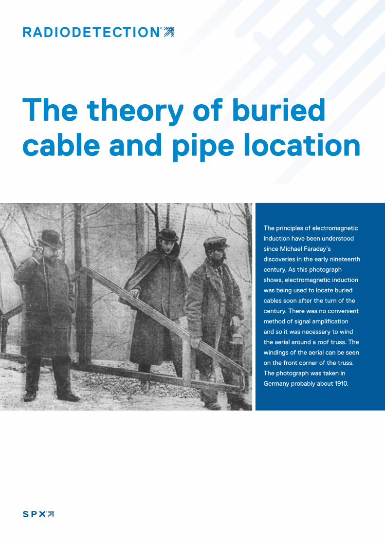
The principles of electromagnetic

induction have been understood

since Michael Faraday’s

discoveries in the early nineteenth

century. As this photograph

shows, electromagnetic induction

was being used to locate buried

cables soon after the turn of the

century. There was no convenient

method of signal amplification

and so it was necessary to wind

the aerial around a roof truss. The

windings of the aerial can be seen

on the front corner of the truss.

The photograph was taken in

Germany probably about 1910.

These notes are intended to give

those involved in the day-to-day

problems of cable and pipe location

an understanding of the principles on

which electromagnetic detection is

based. No theoretical qualifications or

skills are needed to use Radiodetection

equipment successfully, but the addition

of some understanding of what is

actually going on in this invisible world

of magnetic fields will help to increase

the user’s confidence. It will also explain

some of the limitations as well as the

capabilities of this important technique.

Contents Page

Locating buried utility lines 1. Different locating techniques 3

2. Advantages of electromagnetic location 3

Theory of electromagnetic location 3. Basic electromagnetic theory 4

4. Earth return current, AC signals and capacitance 5

5. Active and passive signals 6

6. Passive signals 7

7. Active signal application 8

8. Tracing non-metallic pipes 10

9. Detection and location of signal sources 11

10. The twin aerial antenna and depth estimation 12

11. CM current measurement 13

12. CD current direction 14

The two most common questions 13. How far can a transmitter signal be traced? 17

14. Accuracy of electromagnetic location technology and Radiodetection locators 19

15. Cable Fault-Finding 21

3

1 Different locating techniques 2 Advantages of electromagnetic location

Information is a most important ingredient in any undertaking. It permits planning an afternoon’s work or planning a multimillion dollar enterprise.

The difficulty of obtaining information about buried utility lines is that nothing is visible. Drawings, plans or information should always be obtained but they may be faulty or incomplete. A suitable technique has to be used to obtain the information from underground and a number of methods are available:

Ground Penetrating Radar

In some ground conditions GPR has certain advantages over alternative techniques because of its ability to ‘see’ non-metallic objects as well as metallic ones. However, GPR products tend to be bigger and more expensive, and can require increased levels of training to get the most from the equipment. Surveys can also take longer than with other methods, putting them beyond the scope of many operators.

Sonic surveying

Injection of sound or ultra-sonic waves into the ground or along a line is a technique for tracing plastic water pipes but is not suitable for locating other buried services.

Note: Line is a continuous metal pipe, cable or other conductor capable of carrying an electric current.

Dowsing

Technique, yes and certainly the oldest, but technology – no. Although the hazel twig and all its variants continue to be used with varying effect by practitioners of these obscure but interesting arts, ease of handling is the only one of its features which can be claimed with any certainty.

Electromagnetic location

This method of locating buried pipes, cables and sewers has become almost universal. Its main shortcoming is that it will not locate non-metallic lines such as plastic pipes. However, utilities taking the small amount of trouble to lay tracer wires with plastic pipes are not affected by this shortcoming.

The technology has a large number of advantages and Radiodetection specialises in developing and exploiting electromagnetic location technology.

Electromagnetic location combines many advantages and facilities for obtaining information from underground that are not available from any other technique or combination of techniques.

l It can search an area from the surface to locate buried lines.

l It can trace and identify a target line.

l It can trace and identify sewers or other non-metallic ducts or pipes to which there is access; it can locate blockages and collapses.

l It can measure depth from the surface.

l It can monitor the progress of ‘No Dig’ tools and instruments.

l The technology can be used to provide data to steer equipment or tools both above ground and below ground, or on the sea bed.

l It can find some types of cable fault, monitor pipeline coating condition and locate water leaks in plastic pipes.

l It can pinpoint the position of joints in iron gas pipes.

l The equipment is portable.

l The equipment is easily handled and is successfully used by workers.

l The technique works in all soil conditions; even underwater.

l The component parts of the technology are low cost. Sufficiently low cost to be purchased by small contractors or issued on a large scale by regional or national organisations.

l The technology exists today.

The wide variety of functions and applications requires just three basic building blocks:l a signal generator or transmitter to apply a signal to a

buried line.

l a small self-contained transmitter suitable for inserting in drains or ducts.

l a handheld receiver to locate the signals from the transmitters or to locate signals occurring ‘naturally’ on buried lines.

4

3 Basic electromagnetic theory

3.1 The signal, AC or DC?

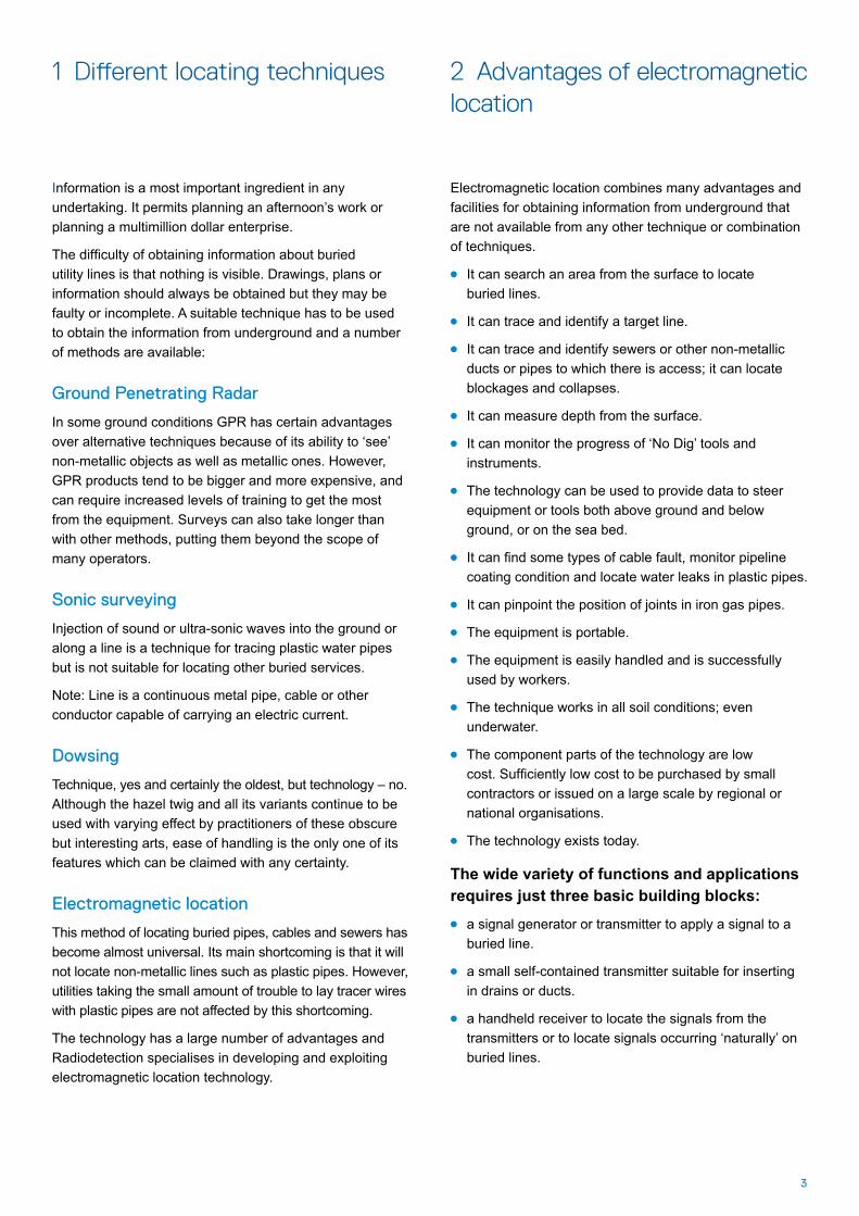
A current flowing along a conductor creates a magnetic field. This magnetic field forms a cylindrical shape around the conductor and is called the ‘signal’. Note that this field is produced by current flowing, and not by voltage.

While it is possible to insulate against the flow of electricity it is not possible to insulate against a magnetic field, and the shape of the field is not changed by cable insulation nor by the presence of different types of soil.

With DC. flowing along the conductor, the field has a constant magnitude and direction, like the permanent magnet of the earth’s magnetic field.

An instrument capable of measuring magnitude and polarity is needed to detect a DC. field. This is not feasible because of the difficulty of measuring a static field against the earth’s magnetic field.

But AC not only gives a field but also an oscillating frequency of reversals, and it is this which makes effective location possible through the principle of electromagnetic induction.

3.2 Electromagnetic induction

If a bar magnet is inserted into a coil of wire a sensitive voltmeter will show a deflection but only while the magnet is moving. As soon as it stops the instrument reads zero. If the magnet is withdrawn quickly the meter deflection will be in the opposite direction – but again only until movement stops.

The quicker the movement, the higher the reading.

The fundamental principle which this illustrates is that of electromagnetic induction: any change of magnetic flux linking a conductor will induce a voltage in it.

Alternating flux is constantly changing, and so induces a corresponding alternating voltage. We use this principle in two ways:

a. To impose a signal onto a buried conductor by subjecting it to a magnetic field set up by an AC signal transmitter in the vicinity, Section 7.

b. To detect a signal in a buried conductor by amplifying the tiny voltages induced by its field in the aerials of a receiver, Section 9.

The rate of change of an alternating voltage is its frequency, i.e. number of positive and negative pulsations, cycles per second, with the SI unit of Hertz (Hz). Just as moving the magnet quicker gave a higher reading, alternating a field at a higher frequency induces a higher voltage for the same field strength.

5

4 Earth return current, AC signals and capacitance

4.1 Capacitance effects

Most people know that an electric circuit has to be completed to allow a current to flow. So how can a low powered signal source at the surface make a detectable current flow in a properly insulated buried conductor? The voltages available are obviously quite incapable of punching through insulation. The answer lies in the effect of capacitance on AC circuits.

A classic capacitor requires two conductors, but there is only one conductor, the pipe or cable. Where is the other? It is the ground. While each particle of soil, sand or rock seems to have a high resistance, there is so much of it that the ground acts as if there is a conducting layer around the conductor. So the conductor charges up relative to ground.

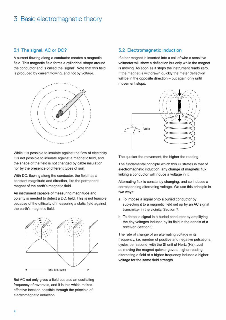
Because a large area of ground is needed to produce this effect, the buried conductor behaves as if it has a string of small capacitors along it. So if AC is applied to the conductor at one point, current will flow out both ways, decreasing in magnitude as more and more leaks away.

The higher the frequency the greater the current because the reactance of the capacitors drop. As the capacitance is effectively distributed along the length of the cable, the signal strength dissipates along the length cable.

Capacitance increases with conductor area, so that surface area of the conductor, and therefore the size of a pipe, affects the distance the signal will carry. The same signal strength will leak away over a much shorter distance from a large pipe than from a small one.

At the opposite end of the scale the capacitance of a small diameter cable may be so low that little or no current will flow and result in too small a signal to be detectable.

The effect of capacitance explains why the signal usually decreases and finally disappears some distance before the end of an insulated conductor that has not been grounded, such as a cable pot end.

ii i i i i

3i 2i i3i2ii

6i

4.2 Ground conductivity

The ability of the ground to pass current will vary locally. Clearly, wet soil is a better conductor than dry sand, and the resulting capacitance effects will vary the apparent conductivity of the conductor. The effect of high ground conductivity is to make it easier to induce current flow and therefore a signal in a buried conductor, because of the good return path. At the same time, the easy return means that the signal becomes lost along a short length of conductor.

Conversely, low ground conductivity requires more energy to induce signal, but it will then be detectable along a greater length of the conductor.

If a buried conductor is in direct contact with the ground, e.g. where a pipeline wrapping has been penetrated, the signal current will leak away by direct conduction.

4.3 Effects of AC frequency

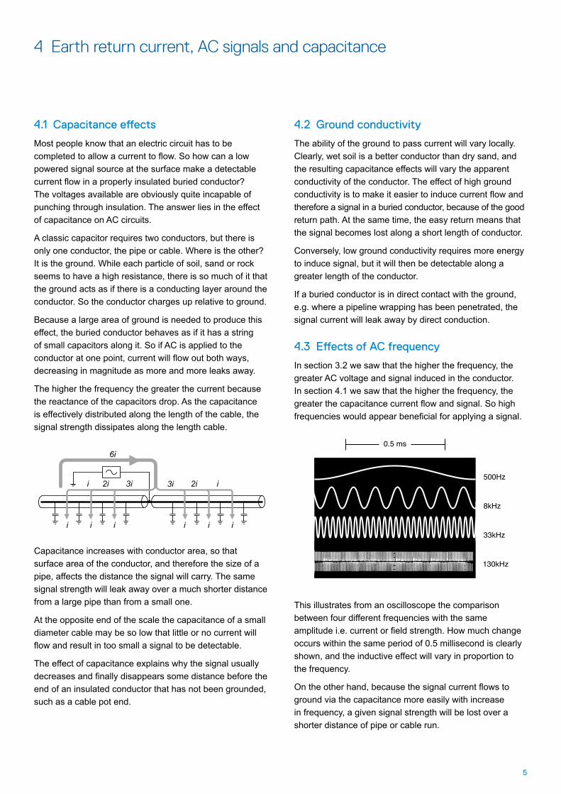
In section 3.2 we saw that the higher the frequency, the greater AC voltage and signal induced in the conductor. In section 4.1 we saw that the higher the frequency, the greater the capacitance current flow and signal. So high frequencies would appear beneficial for applying a signal.

This illustrates from an oscilloscope the comparison between four different frequencies with the same amplitude i.e. current or field strength. How much change occurs within the same period of 0.5 millisecond is clearly shown, and the inductive effect will vary in proportion to the frequency.

On the other hand, because the signal current flows to ground via the capacitance more easily with increase in frequency, a given signal strength will be lost over a shorter distance of pipe or cable run.

6

A further drawback of high frequencies is the ease with which signals aimed at the target conductor can also be coupled by mutual induction to other conductors in the vicinity. This often makes it more difficult to trace a target conductor in a congested area.

4.4 Practical implications of capacitance, ground conductivity and AC frequency

Wherever there is direct electrical contact between line and ground, there will also be signal coupling; both forms of coupling will be reduced if the ground conductivity is low, e.g. dry sandy soil. This is not just because the higher resistance reduces the current flowing via electrical contact; it also reduces the capacitance effect, because while one side of the capacitor (the line) is a good conductor, the surrounding surface presented to it is a poor conductor, so that a much lower ‘charge’ can be stored at any moment than the equivalent volume of wet soil.

While the conductivity of a point of contact between line and ground is not affected by frequency, the fact that the effective impedance of the line to the signal is a combination of resistance and capacitance (as well as a little inductance, which can be ignored at this point) means that it is always easier to couple a high frequency signal into a given line than a low frequency one.

5 Active and passive signals

There are two types of signals from buried conductors which we refer to as ‘passive’ and ‘active’ signals.

5.1 Passive signals

These are ‘naturally’ present in many conductors without any action by the user. Obvious examples are power cables which carry currents as part of their normal duty. Less obvious perhaps is the fact that the earth is full of power system return currents, which will tend to flow along the convenient paths of lower resistance provided by metal pipes and cable sheaths. Even less obvious are radio frequency currents resulting from long wave radio transmissions which penetrate the ground and again flow along buried pipes and cables, whether electrically live or dead. Passive signals therefore enable conductors to be located, but not identified, because the same signals may appear on any conductor.

But there are one or two points to note particularly about passive power signals which may not be immediately obvious. The first one relates to voltage on the line; the signal strength has nothing whatever to do with voltage. Referring to 3.1, it is the current flowing which produces the magnetic field, which is then detected by the locator. If the line is live at high voltage, but its load is switched off, there is nowhere for current to flow, and therefore no detectable power signal, but it remains a potential danger. The second point is that the relationship between load current and signal strength is not direct: any well-designed cable attempts to minimise the strength of radiated electromagnetic field by so twisting the cores that the ‘go’ and ‘return’ current fields largely cancel out.

A third point is that all passive signals are liable to change without notice, so that they cannot be relied upon for such precision requirements as depth measurement. Their great virtue is in enabling buried lines to be detected and avoided using only a simple receiving instrument.

7

5.2 Active signals

These result from deliberate action by the user to connect or induce a known AC signal from a signal transmitter onto a target line. Active signals not only enable buried lines to be located; they also enable them to be positively identified and traced amongst others in a congested situation typical of below-street services in a city.

The fact that the source of the signal is under the operator’s control enables more precise work such as depth measurement and signal strength comparison to be undertaken. In addition, the choice of frequency can be made to suit the job situation, particularly when a multi-frequency signal transmitter is utilised.

5.3 Passive and active location

Only a receiving instrument is required for passive location. This is a great convenience, as it implies very simple operation. It enables a digging crew to be provided with a simple-to-use locator which will enable them to avoid striking buried lines, and thus give them considerable protection against accidental contact with a live power cable, as well as avoiding the consequential disruption and loss from severance of a line.

Active location implies a two part locator, a transmitter and a receiver. Use of active location is essential if target lines are to be positively identified and traced.

5.4 Advantages of combining passive and active signals in a locator

Radiodetection locators combine both passive and active forms of location; choice is by simple switch setting and use of a separate transmitter for active work.

Combining the two modes in a single set of equipment gives the user many possibilities. For instance, lines located during a passive sweep can then each be traced with an active signal to a point where they can be identified. When an excavation is planned to a line that has been located and identified with an active locator, the area can be given a passive sweep to check if there are any other nearby lines that are at risk of being damaged during the excavation.

6 Passive signals

6.1 Electrical power frequencies

A cable carrying AC power produces its own signal at 50-60Hz frequencies, together with higher frequency harmonics thus providing a basis for search and location by a passive receiver.

However, the ground is full of power frequency currents flowing between the ground connection points of power systems and cables. These currents automatically take the paths offering least resistance, which of course are all the buried metallic lines and conductors. They will also be coupled into them by capacitance and induction. The result is therefore that 50-60Hz signals, and their harmonics which are strong up to about 3kHz, are present not only on the majority of buried cables, but also on a large number of pipes or other conductors in the vicinity. This implies that it is possible to locate conductors carrying power frequency signals but not to identify them by passive signal location. The signals may be from a live cable, a pipe or simply from reinforcing bars in concrete, but you will know that a conductor is there. Single phase power cables generally radiate clear signals, but with 3 phase cables the signal is largely the result of imbalance between the phase loads, as balanced currents tend to cancel their fields.

The better the balance, the more difficult detection becomes. As high voltage cable loadings are generally better balanced, a simple passive search in ‘P’ mode might easily detect a street lighting cable whilst missing an 11kV main power cable nearby, and live but unloaded cables which radiate no power signal. This is why the availability of the Radio mode (6.2) is such a valuable complement to the Power mode.

6.2 Radio frequencies

Very low frequency (long wave) radio energy from distant transmitters is present in the atmosphere world-wide. The ground provides return paths for this radiation, and buried metallic lines form preferred paths. They then act as aerials re-radiating these signals. The signal strength will vary with coupling to ground, size of line and soil conductivity, the strongest signals emanating from lines with good grounding at each end, or of substantial length so that capacitance coupling is maximised.

8

These radio frequency signals enable the presence of the conductor to be detected by Radiodetection locators in the Radio mode, which can then find dead power cables or well-balanced high voltage cables which could well be missed by power-frequency-only detectors.

Telecommunication cables and metal pipes also carry these VLF radio signals, so again passive location is effective, but, as with all passive signals, there is no way of identifying the line.

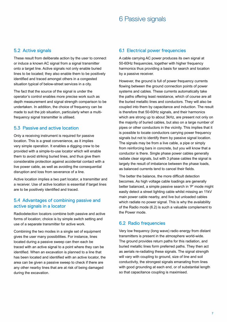
Here is the result of spectrum analysis of the range of frequencies detectable on a typical buried telephone cable, the vertical scale showing the relative signal strength at the frequency shown horizontally. While there is a general broad scatter of frequencies, the two peaks at 16 and 19.6 kHz provide clear tracers for detection by appropriately tuned receivers.

7 Active signal application

Active signal application requires the use of a signal transmitter designed to produce from battery power an a.c. voltage of known frequency and ‘signature’, and the means of applying it to the target buried conductors. The means available are:

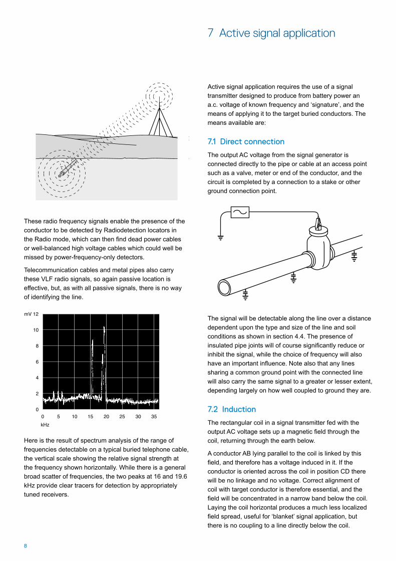
7.1 Direct connection

The output AC voltage from the signal generator is connected directly to the pipe or cable at an access point such as a valve, meter or end of the conductor, and the circuit is completed by a connection to a stake or other ground connection point.

The signal will be detectable along the line over a distance dependent upon the type and size of the line and soil conditions as shown in section 4.4. The presence of insulated pipe joints will of course significantly reduce or inhibit the signal, while the choice of frequency will also have an important influence. Note also that any lines sharing a common ground point with the connected line will also carry the same signal to a greater or lesser extent, depending largely on how well coupled to ground they are.

7.2 Induction

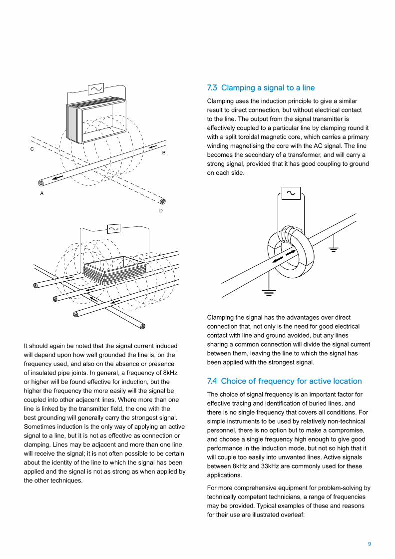
The rectangular coil in a signal transmitter fed with the output AC voltage sets up a magnetic field through the coil, returning through the earth below.

A conductor AB lying parallel to the coil is linked by this field, and therefore has a voltage induced in it. If the conductor is oriented across the coil in position CD there will be no linkage and no voltage. Correct alignment of coil with target conductor is therefore essential, and the field will be concentrated in a narrow band below the coil. Laying the coil horizontal produces a much less localized field spread, useful for ‘blanket’ signal application, but there is no coupling to a line directly below the coil.

9

It should again be noted that the signal current induced will depend upon how well grounded the line is, on the frequency used, and also on the absence or presence of insulated pipe joints. In general, a frequency of 8kHz or higher will be found effective for induction, but the higher the frequency the more easily will the signal be coupled into other adjacent lines. Where more than one line is linked by the transmitter field, the one with the best grounding will generally carry the strongest signal. Sometimes induction is the only way of applying an active signal to a line, but it is not as effective as connection or clamping. Lines may be adjacent and more than one line will receive the signal; it is not often possible to be certain about the identity of the line to which the signal has been applied and the signal is not as strong as when applied by the other techniques.

7.3 Clamping a signal to a line

Clamping uses the induction principle to give a similar result to direct connection, but without electrical contact to the line. The output from the signal transmitter is effectively coupled to a particular line by clamping round it with a split toroidal magnetic core, which carries a primary winding magnetising the core with the AC signal. The line becomes the secondary of a transformer, and will carry a strong signal, provided that it has good coupling to ground on each side.

Clamping the signal has the advantages over direct connection that, not only is the need for good electrical contact with line and ground avoided, but any lines sharing a common connection will divide the signal current between them, leaving the line to which the signal has been applied with the strongest signal.

7.4 Choice of frequency for active location

The choice of signal frequency is an important factor for effective tracing and identification of buried lines, and there is no single frequency that covers all conditions. For simple instruments to be used by relatively non-technical personnel, there is no option but to make a compromise, and choose a single frequency high enough to give good performance in the induction mode, but not so high that it will couple too easily into unwanted lines. Active signals between 8kHz and 33kHz are commonly used for these applications.

For more comprehensive equipment for problem-solving by technically competent technicians, a range of frequencies may be provided. Typical examples of these and reasons for their use are illustrated overleaf:

10

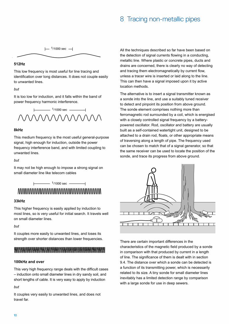
512Hz

This low frequency is most useful for line tracing and identification over long distances. It does not couple easily to unwanted lines.

but

It is too low for induction, and it falls within the band of power frequency harmonic interference.

8kHz

This medium frequency is the most useful general-purpose signal, high enough for induction, outside the power frequency interference band, and with limited coupling to unwanted lines.

but

It may not be high enough to impose a strong signal on small diameter line like telecom cables

33kHz

This higher frequency is easily applied by induction to most lines, so is very useful for initial search. It travels well on small diameter lines.

but

It couples more easily to unwanted lines, and loses its strength over shorter distances than lower frequencies.

100kHz and over

This very high frequency range deals with the difficult cases – induction onto small diameter lines in dry sandy soil, and short lengths of cable. It is very easy to apply by induction

but

It couples very easily to unwanted lines, and does not travel far.

8 Tracing non-metallic pipes

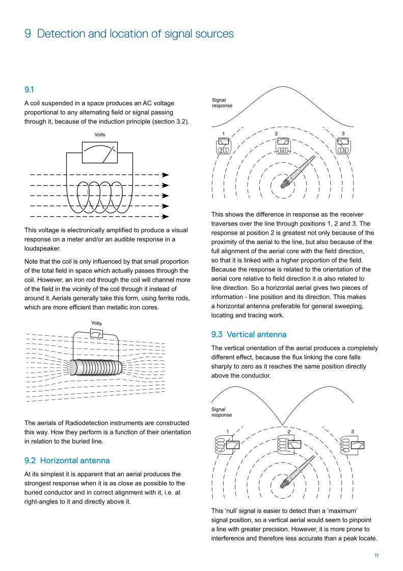
There are certain important differences in the characteristics of the magnetic field produced by a sonde in comparison with that produced by current in a length of line. The significance of them is dealt with in section 9.4. The distance over which a sonde can be detected is a function of its transmitting power, which is necessarily related to its size. A tiny sonde for small diameter lines inevitably has a limited detection range by comparison with a large sonde for use in deep sewers.

All the techniques described so far have been based on the detection of signal currents flowing in a conducting, metallic line. Where plastic or concrete pipes, ducts and drains are concerned, there is clearly no way of detecting and tracing them electromagnetically by current flow, unless a tracer wire is inserted or laid along to the line. This can then have a signal imposed upon it by active location methods.

The alternative is to insert a signal transmitter known as a sonde into the line, and use a suitably tuned receiver to detect and pinpoint its position from above ground. The sonde element comprises nothing more than ferromagnetic rod surrounded by a coil, which is energised with a closely controlled signal frequency by a battery-powered oscillator. Rod, oscillator and battery are usually built as a self-contained watertight unit, designed to be attached to a drain rod, floats, or other appropriate means of traversing along a length of pipe. The frequency used can be chosen to match that of a signal generator, so that the same receiver can be used to locate the position of the sonde, and trace its progress from above ground.

11

9 Detection and location of signal sources

9.1

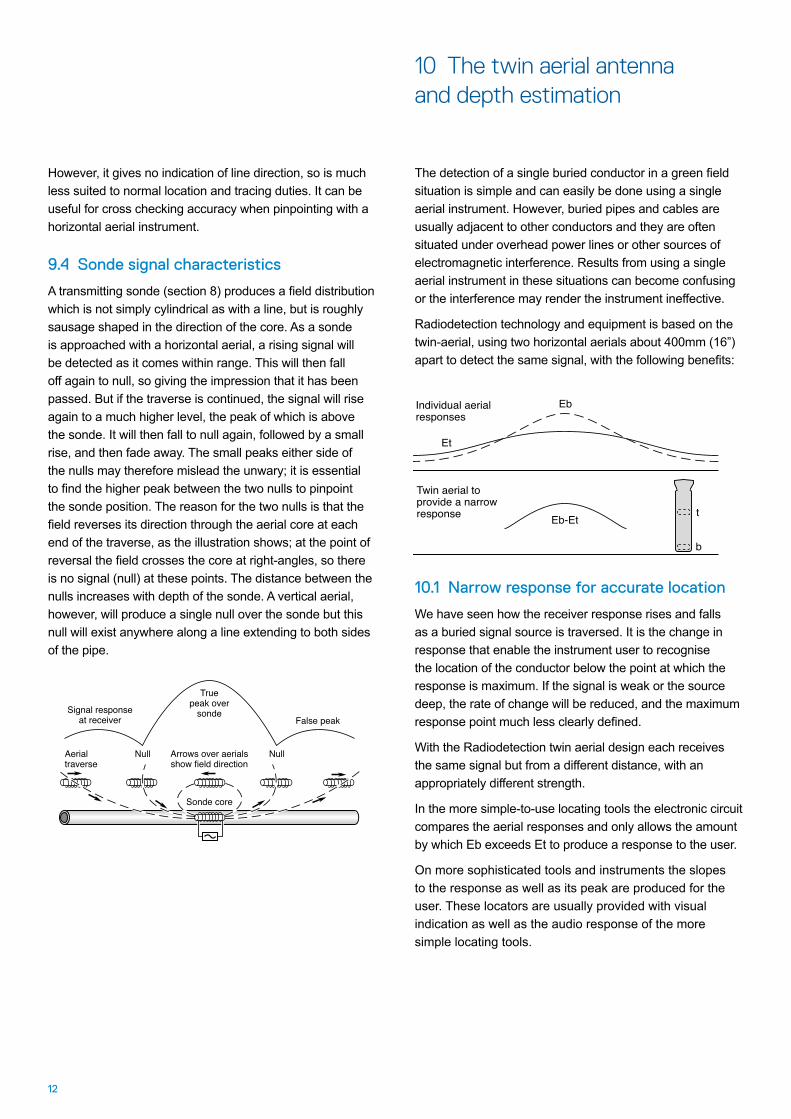
A coil suspended in a space produces an AC voltage proportional to any alternating field or signal passing through it, because of the induction principle (section 3.2).

The aerials of Radiodetection instruments are constructed this way. How they perform is a function of their orientation in relation to the buried line.

9.2 Horizontal antenna

At its simplest it is apparent that an aerial produces the strongest response when it is as close as possible to the buried conductor and in correct alignment with it, i.e. at right-angles to it and directly above it.

This voltage is electronically amplified to produce a visual response on a meter and/or an audible response in a loudspeaker.

Note that the coil is only influenced by that small proportion of the total field in space which actually passes through the coil. However, an iron rod through the coil will channel more of the field in the vicinity of the coil through it instead of around it. Aerials generally take this form, using ferrite rods, which are more efficient than metallic iron cores.

This shows the difference in response as the receiver traverses over the line through positions 1, 2 and 3. The response at position 2 is greatest not only because of the proximity of the aerial to the line, but also because of the full alignment of the aerial core with the field direction, so that it is linked with a higher proportion of the field. Because the response is related to the orientation of the aerial core relative to field direction it is also related to line direction. So a horizontal aerial gives two pieces of information - line position and its direction. This makes a horizontal antenna preferable for general sweeping, locating and tracing work.

9.3 Vertical antenna

The vertical orientation of the aerial produces a completely different effect, because the flux linking the core falls sharply to zero as it reaches the same position directly above the conductor.

This ‘null’ signal is easier to detect than a ‘maximum’ signal position, so a vertical aerial would seem to pinpoint a line with greater precision. However, it is more prone to interference and therefore less accurate than a peak locate.

12

However, it gives no indication of line direction, so is much less suited to normal location and tracing duties. It can be useful for cross checking accuracy when pinpointing with a horizontal aerial instrument.

9.4 Sonde signal characteristics

A transmitting sonde (section 8) produces a field distribution which is not simply cylindrical as with a line, but is roughly sausage shaped in the direction of the core. As a sonde is approached with a horizontal aerial, a rising signal will be detected as it comes within range. This will then fall off again to null, so giving the impression that it has been passed. But if the traverse is continued, the signal will rise again to a much higher level, the peak of which is above the sonde. It will then fall to null again, followed by a small rise, and then fade away. The small peaks either side of the nulls may therefore mislead the unwary; it is essential to find the higher peak between the two nulls to pinpoint the sonde position. The reason for the two nulls is that the field reverses its direction through the aerial core at each end of the traverse, as the illustration shows; at the point of reversal the field crosses the core at right-angles, so there is no signal (null) at these points. The distance between the nulls increases with depth of the sonde. A vertical aerial, however, will produce a single null over the sonde but this null will exist anywhere along a line extending to both sides of the pipe.

10 The twin aerial antenna and depth estimation

The detection of a single buried conductor in a green field situation is simple and can easily be done using a single aerial instrument. However, buried pipes and cables are usually adjacent to other conductors and they are often situated under overhead power lines or other sources of electromagnetic interference. Results from using a single aerial instrument in these situations can become confusing or the interference may render the instrument ineffective.

Radiodetection technology and equipment is based on the twin-aerial, using two horizontal aerials about 400mm (16”) apart to detect the same signal, with the following benefits:

10.1 Narrow response for accurate location

We have seen how the receiver response rises and falls as a buried signal source is traversed. It is the change in response that enable the instrument user to recognise the location of the conductor below the point at which the response is maximum. If the signal is weak or the source deep, the rate of change will be reduced, and the maximum response point much less clearly defined.

With the Radiodetection twin aerial design each receives the same signal but from a different distance, with an appropriately different strength.

In the more simple-to-use locating tools the electronic circuit compares the aerial responses and only allows the amount by which Eb exceeds Et to produce a response to the user.

On more sophisticated tools and instruments the slopes to the response as well as its peak are produced for the user. These locators are usually provided with visual indication as well as the audio response of the more simple locating tools.

13

10.2 Interference rejection

A significant advantage of receiving the signal at two aerials is that their outputs can be compared and analysed. By comparing and rejecting all signals other than those which are stronger at the bottom aerial, the twin aerial instrument can be used to give good results in areas where interference makes a single aerial instrument ineffective.

10.3 Radio mode operation

The twin aerial system also makes it possible to locate conductors re-radiating a VLF radio signal. This radio energy penetrates the soil and is re-radiated by a buried line acting as an aerial. The twin aerial antenna rejects the atmospheric signal which is received at equal strength at each aerial and only accepts the weaker re-radiated signal which is received at greater strength by the bottom aerial.

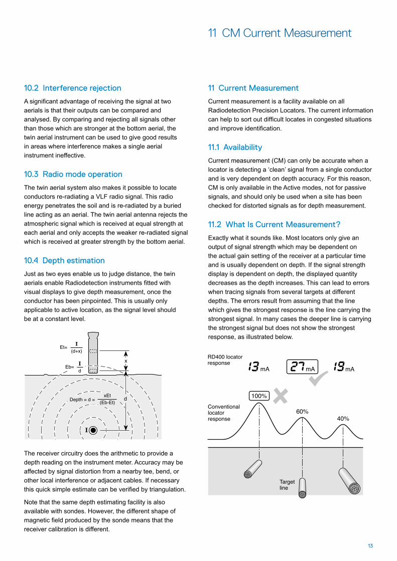
10.4 Depth estimation

Just as two eyes enable us to judge distance, the twin aerials enable Radiodetection instruments fitted with visual displays to give depth measurement, once the conductor has been pinpointed. This is usually only applicable to active location, as the signal level should be at a constant level.

The receiver circuitry does the arithmetic to provide a depth reading on the instrument meter. Accuracy may be affected by signal distortion from a nearby tee, bend, or other local interference or adjacent cables. If necessary this quick simple estimate can be verified by triangulation.

Note that the same depth estimating facility is also available with sondes. However, the different shape of magnetic field produced by the sonde means that the receiver calibration is different.

11 CM Current Measurement

11 Current Measurement

Current measurement is a facility available on all Radiodetection Precision Locators. The current information can help to sort out difficult locates in congested situations and improve identification.

11.1 Availability

Current measurement (CM) can only be accurate when a locator is detecting a ‘clean’ signal from a single conductor and is very dependent on depth accuracy. For this reason, CM is only available in the Active modes, not for passive signals, and should only be used when a site has been checked for distorted signals as for depth measurement.

11.2 What Is Current Measurement?

Exactly what it sounds like. Most locators only give an output of signal strength which may be dependent on the actual gain setting of the receiver at a particular time and is usually dependent on depth. If the signal strength display is dependent on depth, the displayed quantity decreases as the depth increases. This can lead to errors when tracing signals from several targets at different depths. The errors result from assuming that the line which gives the strongest response is the line carrying the strongest signal. In many cases the deeper line is carrying the strongest signal but does not show the strongest response, as illustrated below.

14

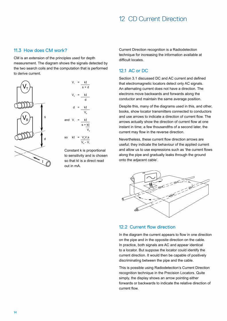
11.3 How does CM work?

CM is an extension of the principles used for depth measurement. The diagram shows the signals detected by the two search coils and the computation that is performed to derive current.

VT = kI s + d

VB = kI d

d = kI VB

and VT = kI s + kI VB

so kI = VBVTs VB - VT

Constant k is proportional to sensitivity and is chosen so that kI is a direct read out in mA.

12 CD Current Direction

Current Direction recognition is a Radiodetection technique for increasing the information available at difficult locates.

12.1 AC or DC

Section 3.1 discussed DC and AC current and defined that electromagnetic locators detect only AC signals. An alternating current does not have a direction. The electrons move backwards and forwards along the conductor and maintain the same average position.

Despite this, many of the diagrams used in this, and other, books, show locator transmitters connected to conductors and use arrows to indicate a direction of current flow. The arrows actually show the direction of current flow at one instant in time; a few thousandths of a second later, the current may flow in the reverse direction.

Nevertheless, these current flow direction arrows are useful; they indicate the behaviour of the applied current and allow us to use expressions such as ‘the current flows along the pipe and gradually leaks through the ground onto the adjacent cable’.

12.2 Current flow direction

In the diagram the current appears to flow in one direction on the pipe and in the opposite direction on the cable. In practice, both signals are AC and appear identical to a locator. But suppose the locator could identify the current direction. It would then be capable of positively discriminating between the pipe and the cable.

This is possible using Radiodetection’s Current Direction recognition technique in the Precision Locators. Quite simply, the display shows an arrow pointing either forwards or backwards to indicate the relative direction of current flow.

15

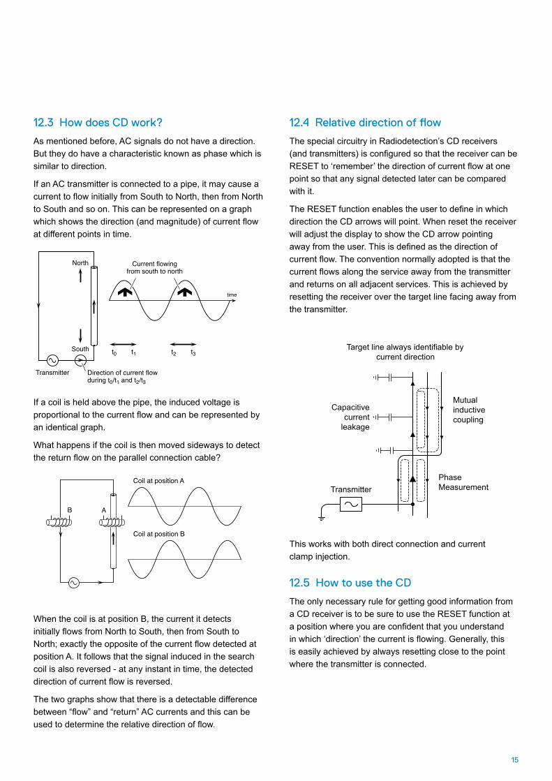
12.3 How does CD work?

As mentioned before, AC signals do not have a direction. But they do have a characteristic known as phase which is similar to direction.

If an AC transmitter is connected to a pipe, it may cause a current to flow initially from South to North, then from North to South and so on. This can be represented on a graph which shows the direction (and magnitude) of current flow at different points in time.

If a coil is held above the pipe, the induced voltage is proportional to the current flow and can be represented by an identical graph.

What happens if the coil is then moved sideways to detect the return flow on the parallel connection cable?

12.4 Relative direction of flow

The special circuitry in Radiodetection’s CD receivers (and transmitters) is configured so that the receiver can be RESET to ‘remember’ the direction of current flow at one point so that any signal detected later can be compared with it.

The RESET function enables the user to define in which direction the CD arrows will point. When reset the receiver will adjust the display to show the CD arrow pointing away from the user. This is defined as the direction of current flow. The convention normally adopted is that the current flows along the service away from the transmitter and returns on all adjacent services. This is achieved by resetting the receiver over the target line facing away from the transmitter.

When the coil is at position B, the current it detects initially flows from North to South, then from South to North; exactly the opposite of the current flow detected at position A. It follows that the signal induced in the search coil is also reversed - at any instant in time, the detected direction of current flow is reversed.

The two graphs show that there is a detectable difference between “flow” and “return” AC currents and this can be used to determine the relative direction of flow.

This works with both direct connection and current clamp injection.

12.5 How to use the CD

The only necessary rule for getting good information from a CD receiver is to be sure to use the RESET function at a position where you are confident that you understand in which ‘direction’ the current is flowing. Generally, this is easily achieved by always resetting close to the point where the transmitter is connected.

Mutual inductive coupling

Capacitive current

leakage

Phase MeasurementTransmitter

Target line always identifiable by current direction

16

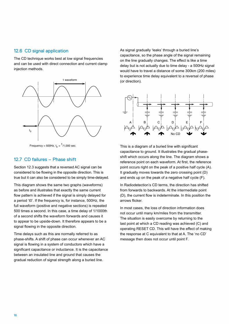
12.6 CD signal application

The CD technique works best at low signal frequencies and can be used with direct connection and current clamp injection methods.

12.7 CD failures – Phase shift

Section 12.3 suggests that a reversed AC signal can be considered to be flowing in the opposite direction. This is true but it can also be considered to be simply time-delayed.

This diagram shows the same two graphs (waveforms) as before and illustrates that exactly the same current flow pattern is achieved if the signal is simply delayed for a period ‘t0’. If the frequency is, for instance, 500Hz, the full waveform (positive and negative sections) is repeated 500 times a second. In this case, a time delay of 1/1000th of a second shifts the waveform forwards and causes it to appear to be upside-down. It therefore appears to be a signal flowing in the opposite direction.

Time delays such as this are normally referred to as phase-shifts. A shift of phase can occur whenever an AC signal is flowing in a system of conductors which have a significant capacitance or inductance. It is the capacitance between an insulated line and ground that causes the gradual reduction of signal strength along a buried line.

As signal gradually ‘leaks’ through a buried line’s capacitance, so the phase angle of the signal remaining on the line gradually changes. The effect is like a time delay but is not actually due to time delay - a 500Hz signal would have to travel a distance of some 300km (200 miles) to experience time delay equivalent to a reversal of phase (or direction).

This is a diagram of a buried line with significant capacitance to ground. It illustrates the gradual phase-shift which occurs along the line. The diagram shows a reference point on each waveform. At first, the reference point occurs right on the peak of a positive half cycle (A). It gradually moves towards the zero crossing point (D) and ends up on the peak of a negative half cycle (F).

In Radiodetection’s CD terms, the direction has shifted from forwards to backwards. At the intermediate point (D), the current flow is indeterminate. In this position the arrows flicker.

In most cases, the loss of direction information does not occur until many km/miles from the transmitter. The situation is easily overcome by returning to the last point at which a CD reading was achieved (C) and operating RESET CD. This will have the effect of making the response at C equivalent to that at A. The ‘no CD’ message then does not occur until point F.

17

13 How far can a transmitter signal be traced?

This is a question most locator users want to ask, and most manufacturers wish to avoid answering! This is not through deviousness, but simply because there is no way of discovering the answer other than by empirical experiment for any given line, for the reasons discussed earlier. A more practical question is, ‘How can the location distance from a transmitter be increased or maximized?’

The distance over which a signal starting with a given current strength will effectively reduce to zero will depend upon the Rate of Signal Loss for that line. The most distant point at which this signal will still be detectable will be a function of Receiver Sensitivity; for the receiver to detect it, some current must be present, and its signal distinguishable above spurious and interfering signals, termed noise. The higher the current, the easier it is to detect.

The rate of signal loss is a nominally fixed value for a particular line and signal frequency. It depends upon its fundamental electrical characteristics like conductivity, capacitance and inductance relative to ground and other metallic lines or structures, which are in turn related to line diameter, insulation, soil type and conductivity.

The possibilities for increasing detection distances are therefore:1. Reduce the rate of signal loss2. Increase the signal current3. Increase the receiver sensitivity

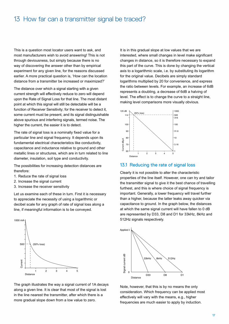
Let us examine each of these in turn. First it is necessary to appreciate the necessity of using a logarithmic or decibel scale for any graph of rate of signal loss along a line, if meaningful information is to be conveyed.

It is in this gradual slope at low values that we are interested, where small changes in level make significant changes in distance, so it is therefore necessary to expand this part of the curve. This is done by changing the vertical axis to a logarithmic scale, i.e. by substituting its logarithm for the original value. Decibels are simply standard logarithms multiplied by 20 for convenience, and express the ratio between levels. For example, an increase of 6dB represents a doubling, a decrease of 6dB a halving of level. The effect is to change the curve to a straight line, making level comparisons more visually obvious.

The graph illustrates the way a signal current of 1A decays along a given line. It is clear that most of the signal is lost in the line nearest the transmitter, after which there is a more gradual slope down from a low value to zero.

13.1 Reducing the rate of signal loss

Clearly it is not possible to alter the characteristic properties of the line itself. However, one can try and tailor the transmitter signal to give it the best chance of travelling furthest, and this is where choice of signal frequency is important. Generally, a lower frequency will travel further than a higher, because the latter leaks away quicker via capacitance to ground. In the graph below, the distances at which the same signal current will have fallen to 0 dB are represented by D33, D8 and D1 for 33kHz, 8kHz and 512Hz signals respectively.

Note, however, that this is by no means the only consideration. Which frequency can be applied most effectively will vary with the means, e.g., higher frequencies are much easier to apply by induction.

18

The background noise level will also differ for different frequencies, particularly within the power frequency harmonic range, and receiver sensitivities may also be affected. There is likely to be an optimum frequency band for any particular line and situation, best established by experiment.

13.2 Increasing the signal current

There are basically three ways of achieving this, costing nothing, a little, and a lot respectively! The one which costs nothing seems obvious, but is often forgotten - make sure there is the best possible ground connection for return of the signal.

The second, which costs a little in equipment design, is to use impedance matching. Any given line will have a fixed impedance at any particular frequency, but its detection will require a certain signal current flow. The voltage required to drive that current through the line will be the product of that current and line impedance seen from the transmitter. For instance, a line impedance of 10 Ohm would require 10V per amp, while an impedance of 200 Ohm would need 200V per amp. If the transmitter is only capable of delivering its full output at a fixed voltage, say 50V, it could drive 5A through the first line, but only 0.25A through the second. So the power transferred into the second line would be much lower than the first (250VA and 12.5VA respectively) while the low impedance line might overload the transmitter at full output. To optimize the transmitter capability, it is clearly desirable to make its output available at more than one voltage/current combination. It is analogous to gear changing, in that the ideal would be an infinitely variable ratio, but practicalities mean that step changes are more economic. Just having two choices gives a considerable advantage over a single voltage capability without increasing the power required.

The third, but costliest, method of increasing current is to increase the transmitter power. Note that a square law applies here, so that in order to double the signal current, a transmitter at four times the power is needed. That not only increases the size, weight and cost of the transmitter elements; it increases the battery drain for portable locators, which then either have a shorter operating time between replacement or recharging, or are larger, heavier, and more costly.

Apart from these practical disadvantages, there is also a safety implication. As we have seen under impedance matching, a high-impedance line may need a high transmitter voltage to impose a significant current on it, and this may take it outside the limits of safe use.

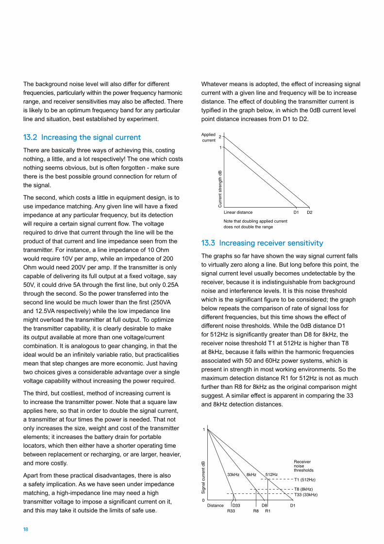
Whatever means is adopted, the effect of increasing signal current with a given line and frequency will be to increase distance. The effect of doubling the transmitter current is typified in the graph below, in which the 0dB current level point distance increases from D1 to D2.

13.3 Increasing receiver sensitivity

The graphs so far have shown the way signal current falls to virtually zero along a line. But long before this point, the signal current level usually becomes undetectable by the receiver, because it is indistinguishable from background noise and interference levels. It is this noise threshold which is the significant figure to be considered; the graph below repeats the comparison of rate of signal loss for different frequencies, but this time shows the effect of different noise thresholds. While the 0dB distance D1 for 512Hz is significantly greater than D8 for 8kHz, the receiver noise threshold T1 at 512Hz is higher than T8 at 8kHz, because it falls within the harmonic frequencies associated with 50 and 60Hz power systems, which is present in strength in most working environments. So the maximum detection distance R1 for 512Hz is not as much further than R8 for 8kHz as the original comparison might suggest. A similar effect is apparent in comparing the 33 and 8kHz detection distances.

19

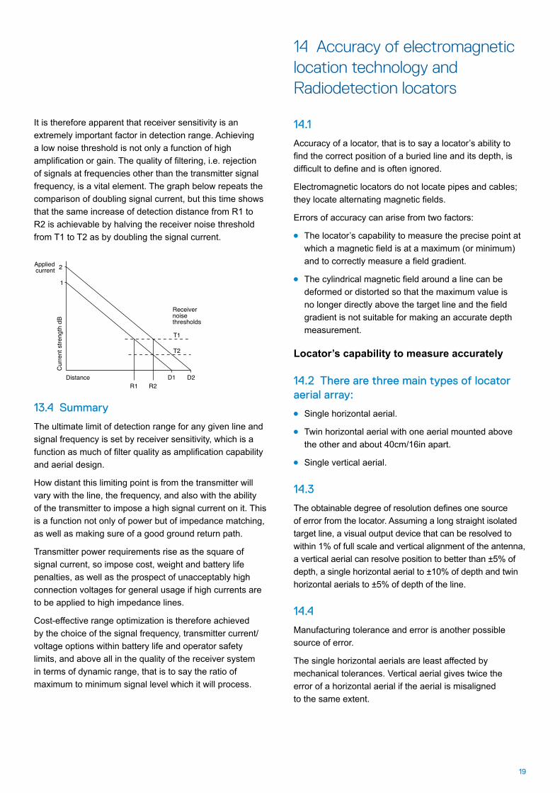
It is therefore apparent that receiver sensitivity is an extremely important factor in detection range. Achieving a low noise threshold is not only a function of high amplification or gain. The quality of filtering, i.e. rejection of signals at frequencies other than the transmitter signal frequency, is a vital element. The graph below repeats the comparison of doubling signal current, but this time shows that the same increase of detection distance from R1 to R2 is achievable by halving the receiver noise threshold from T1 to T2 as by doubling the signal current.

14.1

Accuracy of a locator, that is to say a locator’s ability to find the correct position of a buried line and its depth, is difficult to define and is often ignored.

Electromagnetic locators do not locate pipes and cables; they locate alternating magnetic fields.

Errors of accuracy can arise from two factors:

l The locator’s capability to measure the precise point at which a magnetic field is at a maximum (or minimum) and to correctly measure a field gradient.

l The cylindrical magnetic field around a line can be deformed or distorted so that the maximum value is no longer directly above the target line and the field gradient is not suitable for making an accurate depth measurement.

Locator’s capability to measure accurately

14.2 There are three main types of locator aerial array:

l Single horizontal aerial.

l Twin horizontal aerial with one aerial mounted above the other and about 40cm/16in apart.

l Single vertical aerial.

14.3

The obtainable degree of resolution defines one source of error from the locator. Assuming a long straight isolated target line, a visual output device that can be resolved to within 1% of full scale and vertical alignment of the antenna, a vertical aerial can resolve position to better than ±5% of depth, a single horizontal aerial to ±10% of depth and twin horizontal aerials to ±5% of depth of the line.

14.4

Manufacturing tolerance and error is another possible source of error.

The single horizontal aerials are least affected by mechanical tolerances. Vertical aerial gives twice the error of a horizontal aerial if the aerial is misaligned to the same extent.

13.4 Summary

The ultimate limit of detection range for any given line and signal frequency is set by receiver sensitivity, which is a function as much of filter quality as amplification capability and aerial design.

How distant this limiting point is from the transmitter will vary with the line, the frequency, and also with the ability of the transmitter to impose a high signal current on it. This is a function not only of power but of impedance matching, as well as making sure of a good ground return path.

Transmitter power requirements rise as the square of signal current, so impose cost, weight and battery life penalties, as well as the prospect of unacceptably high connection voltages for general usage if high currents are to be applied to high impedance lines.

Cost-effective range optimization is therefore achieved by the choice of the signal frequency, transmitter current/ voltage options within battery life and operator safety limits, and above all in the quality of the receiver system in terms of dynamic range, that is to say the ratio of maximum to minimum signal level which it will process.

14 Accuracy of electromagnetic location technology and Radiodetection locators

20

Magnetic field distortion

14.5

Most of the problems of accurate location of buried lines in the highway are due to situations that distort magnetic fields. While there are an almost infinite number of ways that fields may be distorted by other lines at various angles and carrying various signals, a useful analysis of accuracy can be obtained by considering just two specific situations:

l A 90° bend in the line.

l Two close parallel lines carrying equal signals or currents. Equal signal currents are, of course, an unlikely eventuality but the example serves as a useful reference for comparison.

14.6

Distortion close to a 90° bend: a locator starts giving faulty information as it comes under the influence of the magnetic field of the perpendicular part of the target line.

Error is expressed as a percentage of the depth d of the line. Relevant distances are expressed in units of d. Measurement of two types of error are useful; maximum degree of plan location error and the length of line along which location error exceeds 10% of depth.

Vertical aerial. A null locator traces a path that is outside the actual bend. The only point where the reading is correct is exactly over the point of the right angle bend. Maximum error is at a point 0.7d from the bend and amounts to 33%. 10% error band extends 5d either side of the bend.

Horizontal aerial. The locator traces a path that cuts across the inside of the bend. Maximum error occurs at the point of the bend and is 25%. 10% error band only extends 0.5d from the bend.

Twin horizontal aerials. Similar to the single horizontal aerial locator, it traces a path to the inside of the bend with a maximum error of 16% and the band of the 10% error is only 0.33d.

14.7

Distortion due to parallel lines buried close together:

a. Similar strength signals on parallel lines following the same direction:

Vertical aerial. Error of less than 10% is only achievable if lines are more than 10d apart. The error will indicate

the lines are closer together. If the lines are closer than 2d there will be a single null in the centre of the lines rather than two separate indications.

Horizontal antenna. Locator indicates lines are closer together but separate indication of each line is possible down to separation of 1.2d when error will be up to 60%. Accuracy of better than 10% is possible if separation is twice depth or greater.

Twin horizontal antenna. Error of 50% at a separation is greater than 1.5d.

b. If similar strength signals on parallel lines run in opposite directions the following may be expected:

Vertical aerial. The locator will show two positions outside the actual position of the lines. It will still show two separate responses even if lines are almost touching and error will be 100%. Accuracy better than 10% is only possible if the two lines are nearly 10d apart.

Horizontal aerial. The locator gives response outside the true positions but with maximum error of 60%. Error falls to 10% when lines are 1.7d apart. There is a sharp null response between lines.

Twin horizontal aerial. Similar response to the single horizontal antenna but a maximum error of 50% reducing to 10% error when separation is 1.2d.

14.8 The above data indicates several conclusions:

The vertical aerial locator gives responses unacceptably wide from the actual position of lines when more than one line with the same signal is present in a small area.

Twin horizontal aerial system provides the best and the most useful response.

Comparison of responses from vertical and horizontal aerials can be used to determine if interference fields are affecting accurate location. Interference is present if the responses from the two systems do not coincide.

This comparison permits multi-aerial instruments such as Radiodetection Precision locators to check if a response is accurate and if the signal is suitable for making an accurate depth measurement.

21

15.1 Reason for using Fault Finding

Cables have outer insulating jackets as a means of preventing water or moisture from getting into the cable. Water needs to be kept out because it creates noise on telephone lines and potential faults on power cables. The main problem is not that the water itself causes electrical failure – the internal conductors of the cable have their own insulation which should prevent this – but that ground water is frequently slightly acidic. This acid may eventually damage the insulation of individual conductors.

The actual fault caused by water in a cable may be found by any of several techniques such as impedance bridge measurements or Pulse/Echo (TDR) techniques. These will find the faulty conductors and enable repair of the service but may not find the actual cause of the fault.

If a fault is caused by moisture ingress through the outer jacket to the sheath, the actual fault may occur some distance from the sheath fault because water runs along the cable to a local low-point; the electrical fault is found at the low point rather than at the sheath fault.

Finding and repairing a sheath fault is sensible preventative maintenance which may reduce recurring faults.

A sheath fault is often caused by physical third-party damage to a cable and often accompanies other damage internal to the cable.

15.2 Principle

Radiodetection locators can find sheath faults. The sheath is intended to be insulated from ground (except at deliberate terminations) so the FFL’s function is to find the point where an otherwise insulated conductor is in electrical contact with the ground.

15 Cable Fault-Finding

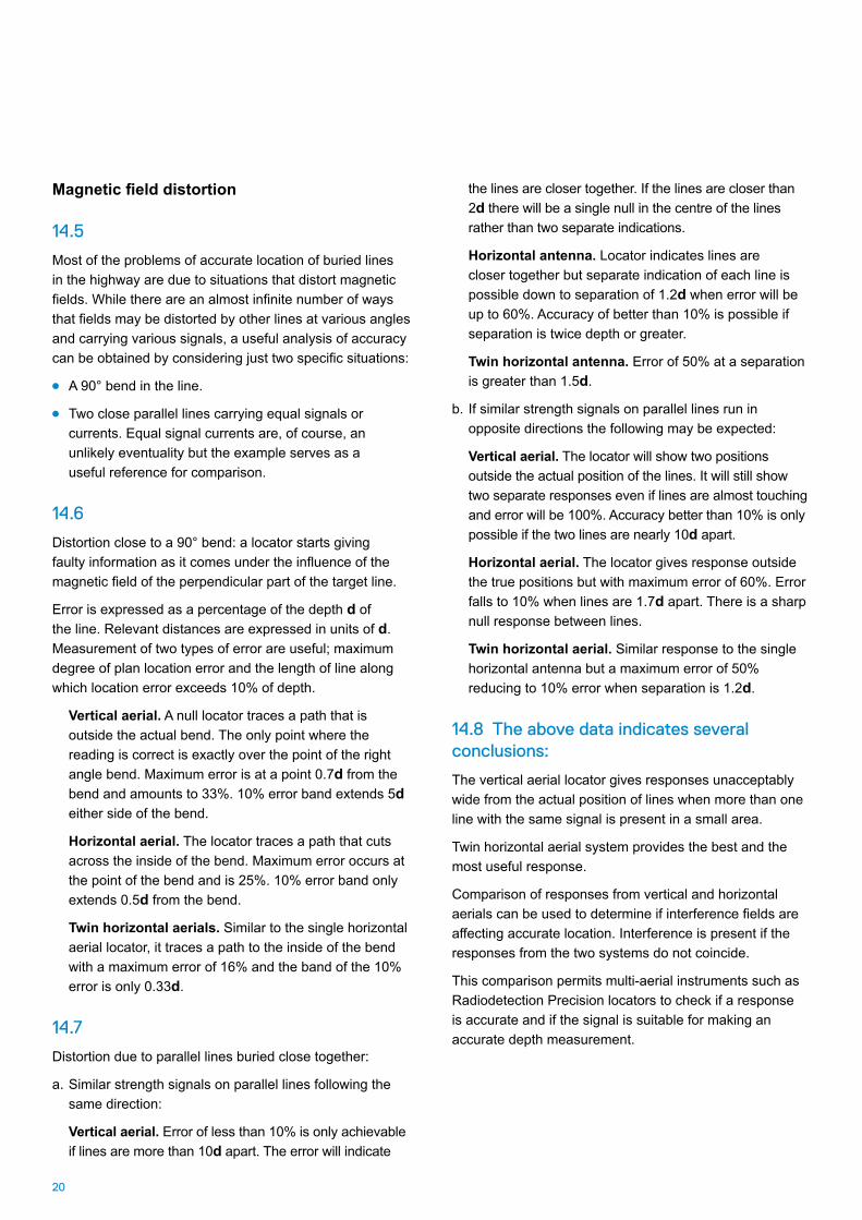
The principle is based on the direction of flow of ground currents.

Consider a battery connected across a faulty sheath and ground and all deliberate ground/sheath connections removed, the path of the current flow will be along the cable sheath to the fault, through the fault to ground and then through the ground back to the other terminal of the battery.

At the sheath fault, the current is ‘escaping’ to ground and will immediately spread out and return to the battery via many different routes.

The current can be pictured flowing out of the fault in every direction so that in the vicinity of the fault the ground currents on the surface radiate out from the fault like the spokes of a wheel.

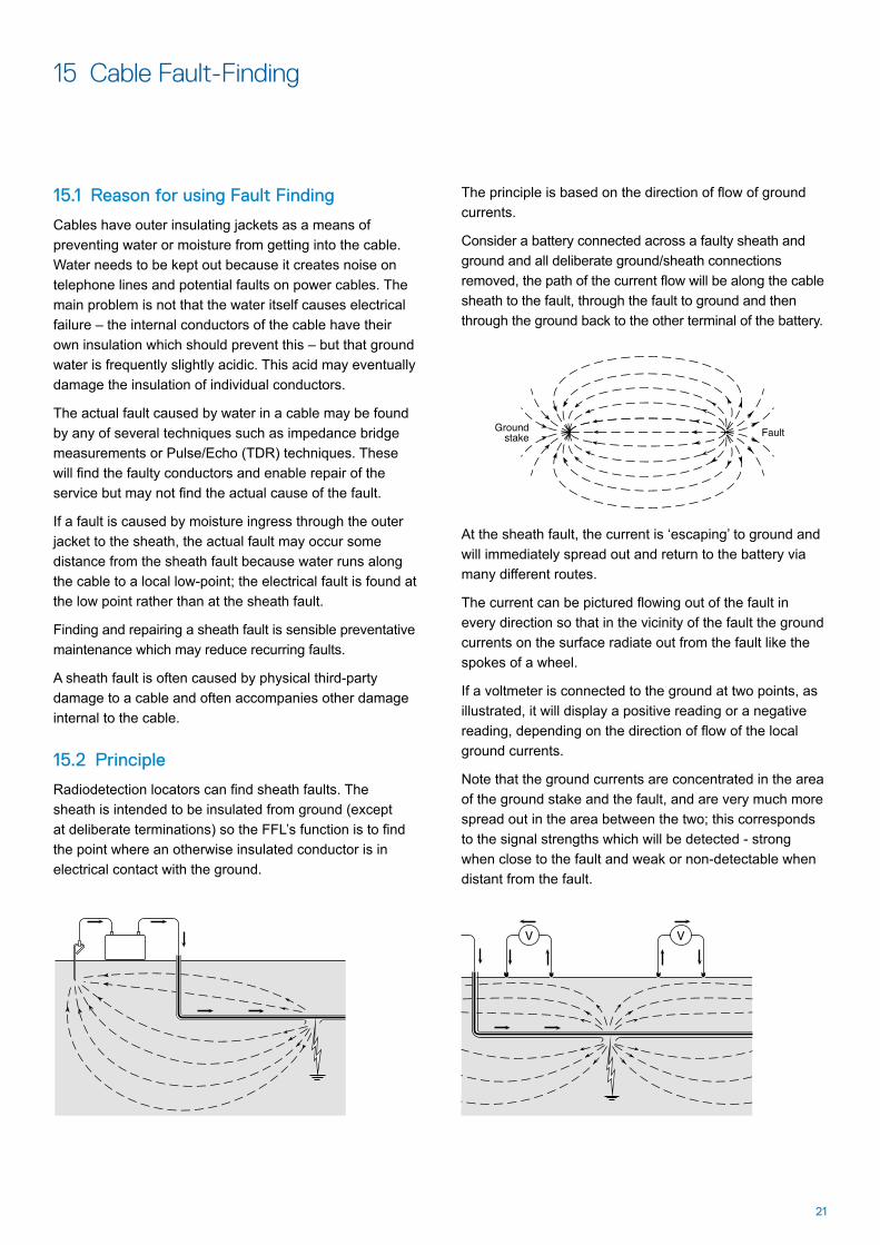
If a voltmeter is connected to the ground at two points, as illustrated, it will display a positive reading or a negative reading, depending on the direction of flow of the local ground currents.

Note that the ground currents are concentrated in the area of the ground stake and the fault, and are very much more spread out in the area between the two; this corresponds to the signal strengths which will be detected - strong when close to the fault and weak or non-detectable when distant from the fault.

22

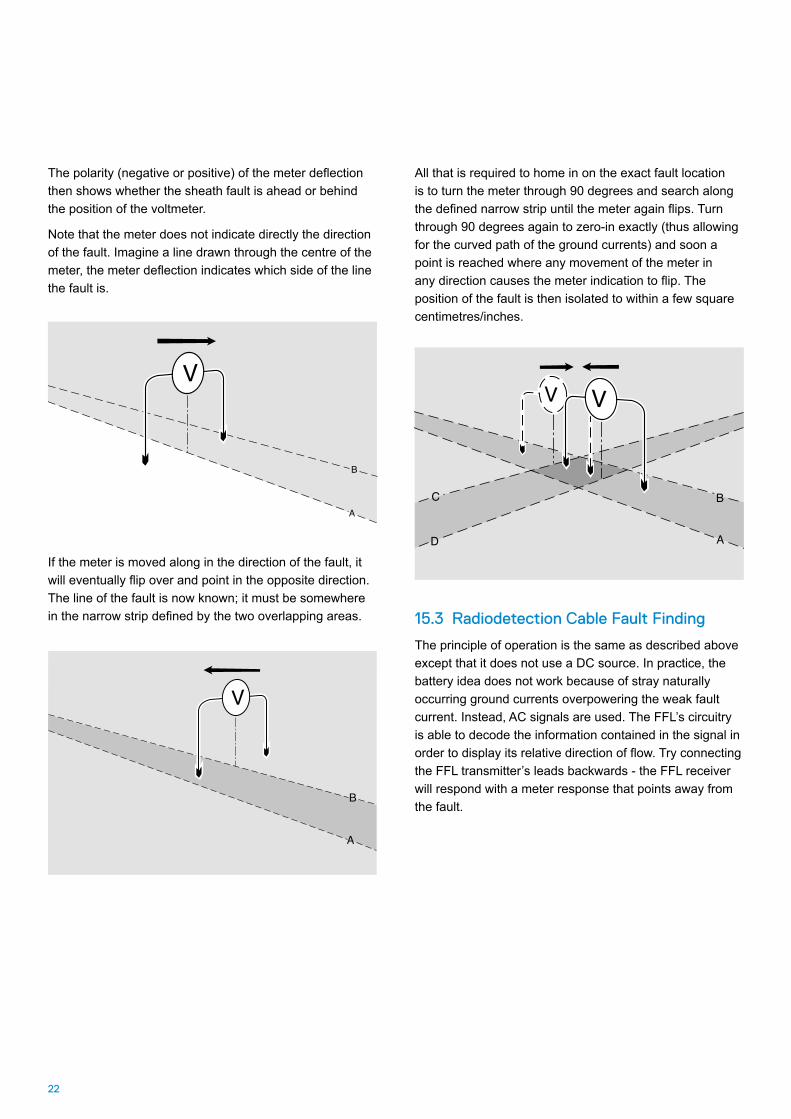
The polarity (negative or positive) of the meter deflection then shows whether the sheath fault is ahead or behind the position of the voltmeter.

Note that the meter does not indicate directly the direction of the fault. Imagine a line drawn through the centre of the meter, the meter deflection indicates which side of the line the fault is.

If the meter is moved along in the direction of the fault, it will eventually flip over and point in the opposite direction. The line of the fault is now known; it must be somewhere in the narrow strip defined by the two overlapping areas.

All that is required to home in on the exact fault location is to turn the meter through 90 degrees and search along the defined narrow strip until the meter again flips. Turn through 90 degrees again to zero-in exactly (thus allowing for the curved path of the ground currents) and soon a point is reached where any movement of the meter in any direction causes the meter indication to flip. The position of the fault is then isolated to within a few square centimetres/inches.

15.3 Radiodetection Cable Fault Finding

The principle of operation is the same as described above except that it does not use a DC source. In practice, the battery idea does not work because of stray naturally occurring ground currents overpowering the weak fault current. Instead, AC signals are used. The FFL’s circuitry is able to decode the information contained in the signal in order to display its relative direction of flow. Try connecting the FFL transmitter’s leads backwards - the FFL receiver will respond with a meter response that points away from the fault.

Copyright © 2017 Radiodetection Ltd. All rights reserved. Radiodetection is a subsidiary of SPX Corporation. Radiodetection, and RD8100 are registered trademarks of Radiodetection in the United States and/or other countries. Due to a policy of continued development, we reserve the right to alter or amend any published specification without notice. This document may not be copied, reproduced, transmitted, modified or used, in whole or in part, without the prior written consent of Radiodetection Ltd.

90/010/ENG/9

Radiodetection is a leading global developer and supplier of test equipment used by utility companies to help install, protect and maintain their infrastructure networks.

Global locations

Radiodetection (USA)28 Tower Road, Raymond, Maine 04071, USA Tel: +1 (207) 655 8525 Toll Free: +1 (877) 247 3797 rd.sales.us@spx.com www.radiodetection.com

Pearpoint (USA)39-740 Garand Lane, Unit B, Palm Desert, CA 92211, USA Tel: +1 800 688 8094 Tel: +1 760 343 7350 pearpoint.sales.us@spx.com www.pearpoint.com

Radiodetection (Canada)344 Edgeley Boulevard, Unit 34, Concord, Ontario L4K 4B7, Canada Tel: +1 (905) 660 9995 Toll Free: +1 (800) 665 7953 rd.sales.ca@spx.com www.radiodetection.com

Radiodetection Ltd. (UK)Western Drive, Bristol, BS14 0AF, UK Tel: +44 (0) 117 976 7776 rd.sales.uk@spx.com www.radiodetection.com

Radiodetection (France)13 Grande Rue, 76220, Neuf Marché, France Tel: +33 (0) 2 32 89 93 60 rd.sales.fr@spx.com http://fr.radiodetection.com

Radiodetection (Benelux)Industriestraat 11, 7041 GD ’s-Heerenberg, Netherlands Tel: +31 (0) 314 66 47 00 rd.sales.nl@spx.com http://nl.radiodetection.com

Radiodetection (Germany)Groendahlscher Weg 118, 46446 Emmerich am Rhein, Germany Tel: +49 (0) 28 51 92 37 20 rd.sales.de@spx.com http://de.radiodetection.com

Radiodetection (Asia-Pacific)Room 708, CC Wu Building, 302-308 Hennessy Road, Wan Chai, Hong Kong SAR, China Tel: +852 2110 8160 rd.sales.asiapacific@spx.com www.radiodetection.com

Radiodetection (China)Ming Hao Building D304, No. 13 Fuqian Avenue, Tianzhu Town, Shunyi District, Beijing 101312, China Tel: +86 (0) 10 8416-3372 rd.service.cn@spx.com http://cn.radiodetection.com

Radiodetection (Australia)Unit H1, 101 Rookwood Road, Yagoona NSW 2199, Australia Tel: +61 (0) 2 9707 3222 rd.sales.au@spx.com www.radiodetection.com