arX

iv:a

stro

-ph/

0502

332v

1 1

6 Fe

b 20

05

To appear in the Astrophysical Journal, 20 February 2005

The Strengths of Near-Infrared Absorption Features Relevant to

Interstellar and Planetary Ices

P. A. Gerakines, J. J. Bray, A. Davis, and C. R. Richey

Astro- and Solar-System Physics Program, Department of Physics, University of Alabama

at Birmingham, Birmingham, AL 35294-1170

gerak@uab.edu

ABSTRACT

The abundances of ices in planetary environments have historically been

obtained through measurements of near-infrared absorption features (λ = 1.0–

2.5 µm), and near-IR transmission measurements of materials present in the in-

terstellar medium are becoming more common. For transmission measurements,

the band strength (or absorption intensity) of an absorption feature must be

known in order to determine the column density of an ice component. In the

experiments presented here, we have measured the band strengths of the near-

IR absorption features for several molecules relevant to the study of interstellar

icy grain mantles and icy planetary bodies: CO (carbon monoxide), CO2 (car-

bon dioxide), C3O2 (carbon suboxide), CH4 (methane), H2O (water), CH3OH

(methanol), and NH3 (ammonia). During a vacuum deposition, the sizes of the

near-IR features were correlated with that of a studied mid-IR feature whose

strength is well known from previous ice studies. These data may be used to

determine ice abundances from observed near-IR spectra of interstellar and plan-

etary materials or to predict the sizes of near-IR features in spectral searches for

these molecules in astrophysical environments.

Subject headings: astrochemistry – molecular data – methods: laboratory –

ISM: abundances – ISM: molecules – planets and satellites: general – comets:

general

1. Introduction

Observations in the mid-infrared spectral region (ν = 4000-400 cm−1; λ = 2.5-25 µm)

have led to the identification of various molecules in the icy mantles that coat the dust

– 2 –

grains present in the interstellar medium (ISM). These include firm identifications of H2O,

CO, CO2, OCN− (cyanate ion), CH3OH, CH4, and OCS, some reasonable but more tentative

identifications of HCOOH (formic acid), HCOO− (formate ion), H2CO (formaldehyde), and

NH3, and the absorption features of some uncharacterized species such as large organics,

or molecules possibly related to ammonium (Ehrenfreund & Charnley 2000; Whittet 2003;

Gibb et al. 2004, and references therein). Observations of spectral features located in the

near-infrared spectral region (ν = 12500-4000 cm−1; λ = 0.8-2.5 µm) have been widely used

to identify ices in the outer Solar System. Molecules such as H2O, CH4, CO, CO2, and N2

have been identified on planetary bodies such as Pluto, Charon, Triton, and Europa (see a

recent review by Roush 2001 and observations by, e.g., Cruikshank et al. 1998, Quirico et al.

1999, Buie & Grundy 2000, or Grundy et al. 2003). Cometary nuclei are presumed to have

a composition similar to these objects (e.g., Irvine et al. 2000).

In recent years, observations of the ISM have begun to extend into the near-IR spectral

region as well. Observations of interstellar material have been made with instruments such

as SpeX on the Infrared Telescope Facility (IRTF) telescope (Vacca et al. 2004) and other

instruments (e.g., Murakawa et al. 2000; Taban et al. 2003). The instruments designed

for the future James Webb Space Teleacope (JWST) call for an increase in fundamental

near-IR data. The JWST Near Infrared Spectrometer (NIRSpec) will perform observations

from 0.6 to 5 µm at spectral resolutions from 100 to 3000, with the primary objective of

studying the processes of star formation in the ISM of external galaxies (Rauscher et al.

2004). Calculations of ice abundances in star-forming regions could be accomplished with

near-IR data such as ours.

The relative abundances of ice components can provide key pieces of information about

the physical and chemical history of the dense cloud in which the ice species reside. Abun-

dances are obtained by observing the absorption features of a molecule arising from its

allowed vibrational modes. For unsaturated features with small peak optical depths, the

integrated area of an interstellar ice absorption feature scales with the molecule’s abundance

by a constant factor. This factor is called the strength of the absorption feature, and it

is an intrinsic physical parameter of its carrier molecule. As has been shown in many pre-

vious studies (e.g., Gerakines et al. 1995; Kerkhof et al. 1999), the IR band strengths of

most molecules show various degrees of dependence upon environmental factors including

ice temperature, overall ice compostion, or the ice’s crystalline phase.

The method by which the column densities of interstellar ices are determined from their

IR absorption features derives from the Beer-Lambert Law. The fraction of light transmitted

through an interstellar cloud at wavenumber ν is given by Tν = exp(−τν), where the optical

– 3 –

depth (τν) may be expressed as the Beer-Lambert Law in the form:

τν = σν N, (1)

where N is the column density of the absorbing molecule (in cm−2), and σν is the absorption

cross-section (in cm2) at wavenumber ν (in cm−1). Since N is a constant with respect to ν,

equation (1) can be integrated over wavenumber and re-arranged in the form

N =

∫iτν dν

Ai

, (2)

where

Ai =

∫i

σν dν, (3)

and the integrals in equations (2) and (3) are taken over the range of the studied feature

i. The parameter Ai has many names in the literature, including the “band strength,”

“integrated cross-section,” “absolute absorption intensity,” or simply “A-value” of the IR

absorption feature i. As expressed above and as is customary in the astrophysical litera-

ture, band strengths possess units of cm molec−1, although the physical chemistry literature

prefers units such as km mmol−1. The IR absorption features of most molecules of astro-

physical interest have band strengths in the range from about 10−20 to 10−16 cm molec−1

(Hudgins et al. 1993; Gerakines et al. 1995; Kerkhof et al. 1999).

Mid-IR absorption features of molecules are the result of their fundamental vibrational

modes, combinations of the fundamental modes, and their lowest-lying overtones. Near-

IR absorptions are generally not due to fundamental vibrations but to higher overtones or

combinations of fundamentals and their overtones. As a result, the near-IR features of a

certain molecule are usually much weaker than those in the mid-IR. This is demonstrated

in Figure 1, where the combined near- and mid-IR spectra of CO, CO2, C3O2, CH4, H2O,

CH3OH, and NH3 are shown. Note that in each case, the near-IR portion of the spectrum

(ν = 10000-4000 cm−1; λ = 1.0-2.5 µm) has been magnified significantly – from 5 to 100

times – in order to display the near- and mid-IR features on similar scales. Laboratory and

observational studies typically use the much stronger mid-IR absorption features to make

identifications of molecules in astrophysical ices, due to the fact that they are more sensitive

tracers of molecular abundances. However, the mid-IR is not always the best spectral region

in which to make astronomical observations. This is the case for reflectance studies within

the Solar System, since the Solar spectrum peaks in the visible range and the Sun emits a

much higher flux of near-IR photons than mid-IR photons.

In our laboratory, we have the ability to study the composite near-IR and mid-IR

spectrum, from 10000 to 400 cm−1 (1.0 to 25 µm), of our ice samples. This allows us to obtain

– 4 –

spectra of the same ice sample in both the near- and mid-IR ranges almost simultaneously,

and thus spectral characteristics in both regions may be studied for any material of interest.

On-going work from our laboratory (Cook et al. 2002; Richey et al. 2004) has been focused

on measuring the near-IR spectra of thick (∼50 µm) ices that have been highly processed by

UV photons.

In this study, we present the near-IR band strengths of CO, CO2, C3O2, CH4, H2O,

CH3OH, and NH3. H2O, CH3OH, CO, CO2, and CH4 are confirmed components of in-

terstellar icy grain mantles, with H2O dominating most interstellar ice environments (e.g.,

Whittet 2003). These are also ice species found in many icy planetary bodies, including

comets and icy moons such as Europa or Triton (e.g., Roush 2001). Extensive searches

for the absorption features of NH3 ice in interstellar and planetary environments have been

performed, with some varied evidence for their presence (e.g., Gibb et al. 2001; Gurtler

et al. 2002; Taban et al. 2003). The carbon suboxide molecule (C3O2) is of interest to both

interstellar and planetary astronomers because it is formed from solid CO in environments

affected by energetic processing such as particle irradiation by cosmic rays or magnetspheric

particles, or by ultraviolet photolysis (Huntress, Allen, & Delitsky 1991; Brucato et al. 1997;

Gerakines & Moore 2001).

The near-IR band strengths of these molecules were obtained in pure ice samples at

10 K by correlating the growths of the near-IR features with those in the mid IR over the

course of long, slow deposits of these materials from the gas phase. Future work (currently

in the preliminary phase) will include studies of near- and mid-IR reflectance spectra as well

as the calculations of ice optical constants in these spectral ranges.

2. Experimental Methods

The ice creation methods and the experimental system used in this study are very similar

to those in previous studies by, e.g., Hudgins et al. (1993), Gerakines et al. (1995), Kerkhof

et al. (1999), Gerakines et al. (2000), and Gerakines & Moore (2001).

Gases are prepared inside a vacuum manifold and vapor-condensed onto an infrared

transmitting substrate (CsI) mounted in the vacuum chamber (P ≈ 3×10−6 mm Hg at room

temperature). The substrate is cooled by a closed-cycle helium refrigerator (Air Products)

to a temperature of 10 K. The temperature of the substrate is continuously monitored by

a chromel-Au thermocouple and is adjustable by a resistive heater element up to room

temperature. The chamber that houses the substrate is accessible to laboratory instruments

through four ports. Two of these ports are have windows composed of KBr, allowing the

– 5 –

transmission of the infrared beam of the spectrometer. One of the ports contains a window

composed of MgF2 to enable ultraviolet photolysis of the ice samples (this option was not

used for the experiments described in this paper), while the fourth port has a glass window

and is used for visual monitoring.

The sample chamber is positioned within the sample compartment of an FTIR spectrom-

eter (ThermoMattson Infinity Gold) so that the spectrometer’s IR beam passes through the

KBr windows and CsI substrate. The spectrometer system is capable of automatic switching

between the appropriate configurations of sources, detectors, and beam splitters that allow

the acquistion of spectra in either the near IR or mid IR without breaking the dry air purge.

This feature allows the measurement of spectra in each of these two spectral regions for the

same ice sample in a single experiment. Near-IR spectra were obtained over the range from

10000 to 3500 cm−1 (λ = 1.0 to 2.9 µm) and mid-IR spectra 4500 to 400 cm−1 (λ = 2.2 to

25 µm). Some overlap between these ranges allows for cross-calibration of common features

as well as for the concatenation of spectra. The spectra of H2O, NH3, CH3OH, CO2, and

C3O2 were obtained with a resolution of 4 cm−1. The IR spectra of CH4 and CO were taken

at a resolution of 1 cm−1. Absorbance spectra (αν) were calculated from the transmission

data (Tν) by using the relationship αν = − log10

Tν (note that τν = αν ln 10).

A bulb containing the gas to be condensed was prepared on a separate vacuum manifold

and then connected to the high-vacuum system by a narrow tube through a needle valve,

which controlled the gas flow into the high-vacuum system. The tube is positioned to release

the gases just in front of the cold substrate window. Gases were deposited at a rate of about

1-5 µmhr−1. Most deposits spanned several days in order to create ices thick enough to

display detectable near-IR absorptions. No significant contamination by background gases

in the vacuum system (dominated by H2O) was observed, supported by the lack of bulk H2O

features in the IR spectra of the non-H2O samples. However some small amounts of H2O

may be isolated within the CO and CO2 samples, as indicated by sharp features near 3400

and 1600 cm−1 (λ = 2.9 and 6.3 µm) in the mid-IR spectrum shown in Figure 1. As indicated

by Gerakines et al. (1995), the band strengths of CO and CO2 are not significantly affectd

by small relative amounts of H2O in an ice sample.

It is important to note that ice samples created in this manner at 10 K are expected to

be amorphous rather than crystalline. The amorphous nature of our samples was supported

by the IR spectra that were recorded during each sample deposit (see Figure 1).

The gases used and their purities are as follows: CO (Matheson, 99.9%), CO2 (Math-

eson, 99.8%), C3O2 (synthesized), CH4 (Matheson, 99+%), H2O (distilled by freeze-thaw

cycles under vacuum), CH3OH (distilled by freeze-thaw cycles under vacuum), and NH3

(Matheson, 99+%). H2O and CH3OH were purified by freezing with liquid N2 under vacuum

– 6 –

and pumping away the more volatile gases while thawing. Carbon suboxide was prepared

as described in detail by Gerakines & Moore (2001)– who followed the method of Miller &

Fateley (1964) to dehydrate malonic acid in the presence of phosphorus pentoxide (P2O5;

a dessicant). To summarize– the gases produced by heating malonic acid to 413 K (H2O,

CO2, acetic acid, and C3O2) were collected in a liquid N2 trap and the C3O2 was distilled

by thermal transfer into a new bulb in the vacuum manifold.

3. Results

The spectra of pure CO, CO2, C3O2, CH4, H2O, CH3OH, and NH3 were collected

in the near-IR region from 10000-3500 cm−1 (1.0-2.9 µm) and the mid-IR region from 4500-

400 cm−1 (2.2-25 µm) during the slow growth of films at 10 K. Figure 1 displays representative

concatenated spectra (10000-400 cm−1; 1.0-25 µm) of these ice samples. The near-IR regions

in Figure 1 have been magnified for direct comparison to the mid-IR region. Band strengths

were measured by observing the rate of growth of a near-IR feature in relation to that of

a stronger feature in the mid-IR, as described below. The mid-IR features used and their

band strengths are listed in Table 1. The near-IR features observed in the spectra and their

calculated band strengths are listed in Table 2. Figures 2-8 display the selected near-IR

regions of the studied spectra and the curves of growth of the near-IR features.

The integrated absorbance of each feature (in units of cm−1) was measured by integrating

between baseline points on either side of the feature, assuming a linear shape to the baseline

underneath each feature. The error in the feature areas was estimated by integrating across

the same limits when no feature was apparent above the noise level in the infrared spectrum.

For narrow features (∆ν . 10 cm−1), the errors were found to be about 0.005 to 0.01 cm−1,

and larger for wider features (in direct proportion to the width). For this reason, any areas

with measured values below about 0.008 cm−1 were omitted from the fitting procedure (these

points are plotted as open symbols in Figures 2-8).

To determine the relative strengths of two absorption features for a single molecule,

we have examined the relationship between the areas of these bands as the ice is grown.

In principle, one could merely measure a single ice spectrum and determine the relative

strengths of any two features by taking the ratio of their areas. However, since the near-

IR features are much weaker than those in the mid-IR (typically, 10-100 times smaller; see

Figure 1), errors in their measured areas are relatively much higher. By monitoring the

relationship between two given absorption features over the course of a slow deposit, the

systematic errors involved in measuring the areas of the near-IR features are signifcantly

reduced.

– 7 –

For optically thin ice absorptions, we expect that depositing a certain number of mole-

cules will cause a linear increase the areas of both features, where each increase is proportional

to that feature’s band strength– see equation 2. Hence, the initial trend in a plot of feature

area vs. feature area should be a straight line, whose slope corresponds to the ratio of the

band strengths. Multiplying this ratio by the known band strength of the mid-IR feature

(Table 1), the near-IR band strength is obtained. The experimental errors in near-IR band

strengths were obtained by multiplying the standard deviations in the best-fitting slopes by

the mid-IR band strength. Values resulting from the trends displayed in Figures 2-8 are

listed in Table 2.

In the cases of CO, CO2, and CH4, the scaling process was complicated by the fact that

the fundamental features are extremely sharp and become saturated very quickly during the

deposit. For CO (Figure 2), the absorption due to its fundamental vibration at 2137 cm−1

(4.679 µm) becomes too large to be useful after only short deposition times. As a result, we

have used the absorption feature of 13CO at 2092 cm−1 (4.780 µm) to scale the 12CO and13CO near-IR features. The strength of 1.5×10−19 cm per 12CO molecule was used for the

2092 cm−1 (4.780 µm) feature, taking the band strength of the 13CO feature from Gerakines

et al. (1995) and scaling by the terrestrial ratio of 12C/13C of 87. For CO2, the combination

mode at 3708 cm−1 (2.697 µm) was used to scale the near-IR features. For CH4 (Figure 5),

the absorptions due to fundamental modes at 3009 and 1306 cm−1 (3.323 and 7.657 µm)

become too strong to be useful after only short timescales as well. Because of this, the near-

IR features were scaled by the absorption feature located at 2815 cm−1 (3.552 µm), which is

due to its ν2 + ν4 vibration mode. In order to to this, we first determined the band strength

for the 2815 cm−1 (3.552 µm) feature to be A = (1.9±0.1)×10−18 cm molec−1 by scaling it by

the ν2 fundamental mode at 1306 cm−1 (λ = 7.657 µm; A = 7.0×10−18 cm molec−1; Kerkhof

et al. 1999) in the spectrum of a thin sample. The 8405 cm−1 (1.190 µm) feature of CH4

displayed a peculiar growth curve, with no discernible linear trend. Hence, no band strength

is listed for this feature in Table 2.

As observed in Figures 2-8, the trends are initially linear for the ices we have studied. In

some cases, the mid-IR feature used for the x-axis becomes so large that its curve of growth

becomes non-linear (the change in feature area no longer responds linearly to the increase in

the number of molecules). In these cases, the non-linear portions of the data set were omitted

from our fitting process (omitted data points are plotted as open symbols in Figures 2-8).

It may be interesting to note that the non-linear parts of the curve are not always identical

from experiment to experiment. This is especially clear in the two separate deposits of C3O2

(Fig. 4), H2O (Fig. 6), and NH3 (Fig. 8). This may suggest that ice deposition rates or other

characteristics of a single experiment can significantly alter the physical properties of the ice

under study, especially when ices are thicker than about 10 µm. This particular issue has

– 8 –

been discussed in detail previously by Quirico & Schmitt (1997).

4. Comparison to previous studies

Taban et al. (2003) have published values for some of the same near-IR band strengths of

pure H2O, NH3, and CH3OH ices at low temperatures. In general, we find our values to be in

excellent agreement with theirs. They quote A = 1.1×10−18 cm molec−1 for the H2O feature

near 5000 cm−1 (2.0 µm), which is in full agreement with our experimentally determined value

of (1.2±0.1)×10−18 cm molec−1. For NH3, they find a value of A = 9.7×10−19 cm molec−1 for

the band near 4478 cm−1 (2.233 µm), for which we find A = (8.7±0.3)×10−19 cm molec−1. For

CH3OH, they measure A = 5.9×10−19 cm molec−1 for the feature near 4395 cm−1 (2.275 µm),

which is also in good agreement with our measured value of (8.7 ± 0.7)×10−19 cm molec−1

for the 4400 cm−1 (2.273 µm) feature observed here.

Quirico & Schmitt (1997) published absorption coefficients (the fraction of intensity

absorbed per unit thickness of the sample; in cm−1) of the near-IR features of pure CO,

CO2, and CH4 for use in planetary ice studies. The absorption coefficient allows one to

calculate the thickness of a sample from the absorbance value at the peak of a feature. It

is not necessarily straightforward to compare band strengths with absorption coefficients for

ice samples prepared in separate laboratories using different techniques, since one must take

into account the densities of the samples in order to connect column densities to thicknesses.

Ice samples in the Quirico & Schmitt (1997) study were created in a closed cell and not by

vapor deposit. For the sake of a comparison to our study, one must make the rather unsafe

assumption that the ice densities and spectral profiles of our samples are identical to theirs

(they most likely are not identical). In this case, the band strengths of any two features for a

given molecule should scale in the same manner as their absorption coefficients. Taking the

ratios of band strengths from Table 2 for pairs of CO, CO2, and CH4 features and comparing

them to the ratios of their reported absorption coefficients Quirico & Schmitt (1997), we find

that some agree quite well (to within a few percent), but most agree only to within a factor

of 2 or so.

Taban et al. (2003) find that the near-IR spectrum of the line of sight toward the high-

mass protostar W33A is consistent with the known abundances of H2O, CH3OH, and CO

as derived from mid-IR data. They claim the detection of the near-IR features of CH3OH

near 4400 cm−1 (2.273 µm) with an optical depth of about 0.014.

Based on our laboratory data, one should be able to predict the optical depths of near-IR

ice absorptions that could be investigated in various astrophysical objects. Using the widths

– 9 –

and strengths for the two strongest near-IR features of our samples, we have estimated the

their optical depths for some well-studied lines of sight in the ISM (e.g., Gerakines et al. 1999;

Gibb et al. 2000). These estimates are listed in Table 3. Although pure ices at 10 K may

not reflect the most realistic cases for these objects, previous work (Gerakines et al. 1995;

Kerkhof et al. 1999) does suggest that the band strengths of most molecules studied to date

do not vary by more than a factor of 2 or so according to composition or to temperature.

It should be noted that the strengths of a certain molecule’s absorption features do vary

by large amounts when different crystalline states are considered, but interstellar ices are

presumed to be amorphous (e.g., Whittet 2003).

5. Summary and Future Work

In this paper, we have shown that the near-IR band strengths (or “absorption intensi-

ties”) for molecules of interest to both interstellar and planetary astronomers may be deter-

mined through correlations to their better-known mid-IR characteristics. By correlating the

growth of near-IR and mid-IR absorption features for molecules at low temperature, we have

calculated the absorption strengths for the near-IR features of CO, CO2, C3O2, CH4, H2O,

CH3OH, and NH3. These strengths may be used to determine the column densities of these

molecules in the interstellar dense cloud or other environments from observed transmission

data.

This is the first paper in a series of near- and mid-IR correlation studies of ice samples of

astrophysical interest. Future work currently in preparation in our laboratory will involve the

calculation of ice optical constants for use in particle scattering models as well as reflectance

studies for use in the direct interpretation of planetary observations of reflected sunlight.

We will also investigate the effects, if any, of ice composition on the near-IR band strengths

as well as the differences bewteen the near-IR band strengths of crystalline and amorphous

ices.

PAG gratefully acknowledges laboratory start-up funds from the University of Alabama

at Birmingham, financial support through NASA grant number NNG04GA63A, and many

conversations with Marla Moore and Reggie Hudson, who kindly provided comments on an

early version of this manuscript.

– 10 –

REFERENCES

Brucato, J. R., Palumbo, M. E., & Strazzulla, G. 1997, Icarus, 125, 135

Buie, M. W., & Grundy, W. M. 2000, Icarus, 148, 324

Calvani, P., Cunsolo, S., Lupi, S., & Nucara, A. 1992, J. Chem. Phys., 96, 7372

Cook, A. M., Gerakines, P. A., & Saperstein, E. 2002, Bulletin of the American Astronomical

Society, 34, 908

Cruikshank, D. P., et al. 1998, Icarus, 135, 389

d’Hendecourt, L. B., & Allamandola, L. J. 1986, A&AS, 64, 453

Ehrenfreund, P., & Charnley, S. B. 2000, ARA&A, 38, 427

Gurtler, J., Klaas, U., Henning, T., Abraham, P., Lemke, D., Schreyer, K., & Lehmann, K.

2002, A&A, 390, 1075

Gerakines, P. A., & Moore, M. H. 2001, Icarus, 154, 372

Gerakines, P. A., Moore, M. H., & Hudson, R. L. 2000, A&A, 357, 793

Gerakines, P. A., Schutte, W. A., Greenberg, J. M., & van Dishoeck, E. F. 1995, A&A, 296,

810

Gerakines, P. A., et al. 1999, ApJ, 522, 357

Gibb, E. L., Whittet, D. C. B., Boogert, A. C. A., & Tielens, A. G. G. M. 2004, ApJS, 151,

35

Gibb, E. L., Whittet, D. C. B., & Chiar, J. E. 2001, ApJ, 558, 702

Gibb, E. L., et al. 2000, ApJ, 536, 347

Grundy, W. M., Schmitt, B., & Quirico, E. 2002, Icarus, 155, 486

Grundy, W. M., Young, L. A., & Young, E. F. 2003, Icarus, 162, 222

Hudgins, D. M., Sandford, S. A., Allamandola, L. J., & Tielens, A. G. G. M. 1993, ApJS,

86, 713

Huntress, W. T., Allen, M., & Delitsky, M. 1991, Nature, 352, 316

– 11 –

Irvine, W. M., Schloerb, F. P., Crovisier, J., Fegley, B., & Mumma, M. J. 2000, in Protostars

and Planets IV, ed. V. Mannings, A. P. Boss, & S. S. Russell (University of Arizona

Press), 1159

Kerkhof, O., Schutte, W. A., & Ehrenfreund, P. 1999, A&A, 346, 990

Miller, F. A., & Fateley, W. G. 1964, Spectrochimica Acta, 20, 253

Murakawa, K., Tamura, M., & Nagata, T. 2000, ApJS, 128, 603

Quirico, E., Doute, S., Schmitt, B., de Bergh, C., Cruikshank, D. P., Owen, T. C., Geballe,

T. R., & Roush, T. L. 1999, Icarus, 139, 159

Quirico, E., & Schmitt, B. 1997, Icarus, 127, 354

Rauscher, B. J., Figer, D. F., Hill, R. J., Jakobsen, P. J., Moseley, S. H., Regan, M. W., &

Strada, P. 2004, American Astronomical Society Meeting, 204

Richey, C. R., Underwood, R. A., & Gerakines, P. A. 2004, in Lunar and Planetary Institute

Conference Abstracts, 1450

Roush, T. L. 2001, J. Geophys. Res., 106, 33315

Taban, I. M., Schutte, W. A., Pontoppidan, K. M., & van Dishoeck, E. F. 2003, A&A, 399,

169

Vacca, W. D., Cushing, M. C., & Simon, T. 2004, ApJ, 609, L29

Whittet, D. C. B. 2003, Dust in the Galactic Environment, 2nd edn. (Bristol: Institute of

Physics)

This preprint was prepared with the AAS LATEX macros v5.2.

– 12 –

Table 1. Mid-Infrared Features Used in Strength Determinations

Molecule ν [cm−1] λ [µm] A [cm molec−1] Reference

CO 2092 4.780 1.5×10−19 a 1

CO2 3708 2.697 1.4×10−18 1

C3O2 3744 2.671 3.8×10−18 2

CH4 1306 7.657 7.0×10−18 3

2815 3.552 (1.9 ± 0.1)×10−18 4

H2O 1670 5.988 1.2×10−17 1

CH3OH 2830 3.534 7.6×10−18 5

NH3 1070 9.346 1.2×10−17 3

aAlthough this is a feature of 13CO, its band strength is expressed in units of cm per 12CO

molecule.

Note. — (1) Gerakines et al. (1995); (2) Gerakines & Moore (2001); (3) Kerkhof

et al. (1999); (4) determined by scaling the 1306 cm−1 (7.657 µm) feature (see text); (5)

d’Hendecourt & Allamandola (1986).

– 13 –

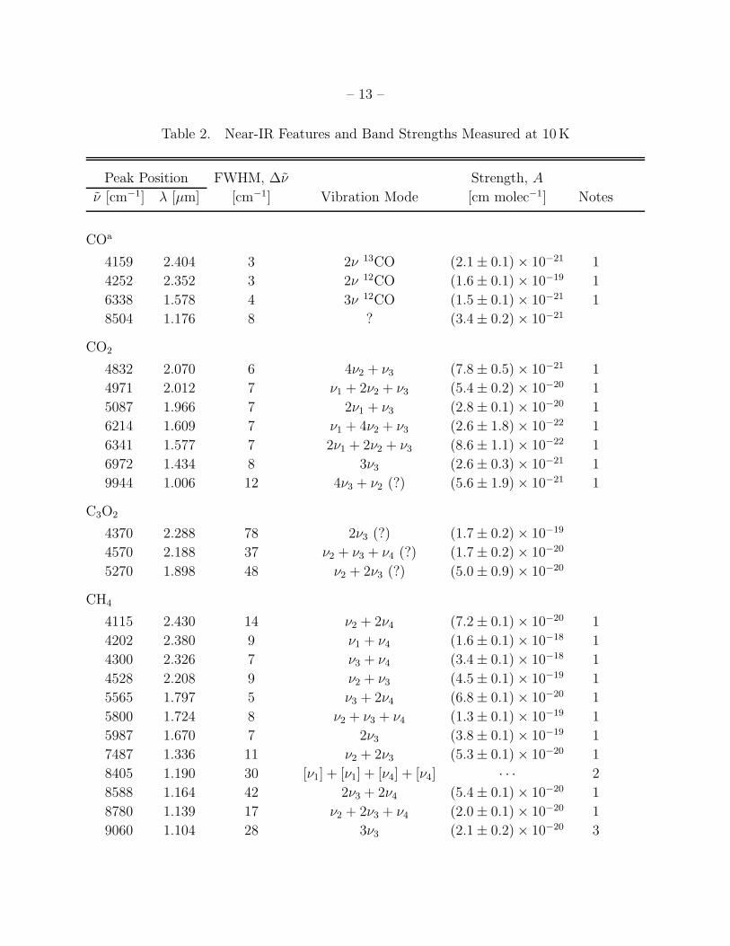
Table 2. Near-IR Features and Band Strengths Measured at 10 K

Peak Position FWHM, ∆ν Strength, A

ν [cm−1] λ [µm] [cm−1] Vibration Mode [cm molec−1] Notes

COa

4159 2.404 3 2ν 13CO (2.1 ± 0.1) × 10−21 1

4252 2.352 3 2ν 12CO (1.6 ± 0.1) × 10−19 1

6338 1.578 4 3ν 12CO (1.5 ± 0.1) × 10−21 1

8504 1.176 8 ? (3.4 ± 0.2) × 10−21

CO2

4832 2.070 6 4ν2 + ν3 (7.8 ± 0.5) × 10−21 1

4971 2.012 7 ν1 + 2ν2 + ν3 (5.4 ± 0.2) × 10−20 1

5087 1.966 7 2ν1 + ν3 (2.8 ± 0.1) × 10−20 1

6214 1.609 7 ν1 + 4ν2 + ν3 (2.6 ± 1.8) × 10−22 1

6341 1.577 7 2ν1 + 2ν2 + ν3 (8.6 ± 1.1) × 10−22 1

6972 1.434 8 3ν3 (2.6 ± 0.3) × 10−21 1

9944 1.006 12 4ν3 + ν2 (?) (5.6 ± 1.9) × 10−21 1

C3O2

4370 2.288 78 2ν3 (?) (1.7 ± 0.2) × 10−19

4570 2.188 37 ν2 + ν3 + ν4 (?) (1.7 ± 0.2) × 10−20

5270 1.898 48 ν2 + 2ν3 (?) (5.0 ± 0.9) × 10−20

CH4

4115 2.430 14 ν2 + 2ν4 (7.2 ± 0.1) × 10−20 1

4202 2.380 9 ν1 + ν4 (1.6 ± 0.1) × 10−18 1

4300 2.326 7 ν3 + ν4 (3.4 ± 0.1) × 10−18 1

4528 2.208 9 ν2 + ν3 (4.5 ± 0.1) × 10−19 1

5565 1.797 5 ν3 + 2ν4 (6.8 ± 0.1) × 10−20 1

5800 1.724 8 ν2 + ν3 + ν4 (1.3 ± 0.1) × 10−19 1

5987 1.670 7 2ν3 (3.8 ± 0.1) × 10−19 1

7487 1.336 11 ν2 + 2ν3 (5.3 ± 0.1) × 10−20 1

8405 1.190 30 [ν1] + [ν1] + [ν4] + [ν4] · · · 2

8588 1.164 42 2ν3 + 2ν4 (5.4 ± 0.1) × 10−20 1

8780 1.139 17 ν2 + 2ν3 + ν4 (2.0 ± 0.1) × 10−20 1

9060 1.104 28 3ν3 (2.1 ± 0.2) × 10−20 3

– 14 –

Table 2—Continued

Peak Position FWHM, ∆ν Strength, A

ν [cm−1] λ [µm] [cm−1] Vibration Mode [cm molec−1] Notes

H2O

5040 1.984 408 ν2 + ν3 (1.2 ± 0.1) × 10−18

6684 1.496 520 2ν3 (8.8 ± 1.0) × 10−19

CH3OH

4280 2.336 34 ? (8.0 ± 0.9) × 10−20

4400 2.273 72 ? (8.7 ± 0.7) × 10−19

NH3

4474 2.235 94 ν1 + ν2 (?) (8.7 ± 0.3) × 10−19

4993 2.002 68 ν1 + ν4 (?) (8.1 ± 0.4) × 10−19

6099 1.640 107 ν1 + ν2 + ν4 (?) (2.8 ± 0.5) × 10−20

6515 1.535 118 2ν1 (?) (3.9 ± 0.3) × 10−20

aAll 12CO and 13CO band strengths are expressed in units of cm per 12CO molecule.

Note. — (1) vibrational mode assignment from Calvani et al. (1992) and Quirico & Schmitt

(1997); (2) combination of dual-phonon modes (Calvani et al. 1992; Quirico & Schmitt 1997);

(3) vibrational mode assignment from Grundy et al. (2002).

– 15 –

Table 3. Column Densitiesa and Predicted Near-IR Optical Depthsb of Interstellar Ices

W33A NGC 7538 IRS9 Elias 16 Sgr A∗

CO

N 8.8×1017 1.2×1018 6.3×1017 <2×1017

τ(2.352 µm) 0.05 0.06 0.03 <0.01

CO2

N 1.4×1018 1.7×1018 4.5×1017 1.8×1017

τ(1.966 µm) 0.006 0.007 0.002 <0.001

τ(2.012 µm) 0.01 0.01 0.004 0.001

CH4

N 1.7×1017 1.5×1017· · · 2.6×1016

τ(2.326 µm) 0.08 0.07 · · · 0.01

τ(2.380 µm) 0.03 0.03 · · · 0.005

H2O

N 1.1×1019 7.5×1018 2.5×1018 1.3×1018

τ(1.496 µm) 0.02 0.01 0.004 0.002

τ(1.984 µm) 0.03 0.02 0.007 0.004

CH3OH

N 2.0×1017 3.8×1017 <8×1016 <5×1016

τ(2.273 µm) 0.02 0.005 <0.01 <0.006

τ(2.336 µm) 0.005 <0.001 <0.002 <0.001

aColumn densities (N) have units of cm−2; from Gibb et al. (2000).

bOptical depths have been calculated from the listed column densities, using width and

strength data listed in Table 2.

– 16 –

Fig. 1.— Combined near- and mid-IR spectra (10000-400 cm−1; 1.0-25 µm) of pure samples

at 10 K for the seven molecules studied. In each case, the near-IR portion of the spectrum

(10000-4000 cm−1; 1.0-2.5 µm) has been magnified by the amount indicated in the Figure.

The sinusoidal appearance of the CO near-IR spectrum is due to interference of the spec-

trometer’s IR beam within the sample. Gas-phase H2O lines from the imperfect spectrometer

purge (5540-4100 cm−1 and 7420-7000 cm−1) have been removed from the near-IR spectra of

CO and CH4. The 10000-7000 cm−1 region has been omitted from the near-IR spectra of

C3O2 and CH3OH for clarity, since they are dominated by noise.

Fig. 2.— (top) Selected near-IR absorbance spectra of an 18 µm thick CO ice at 10 K for the

regions surrounding the features studied; (bottom) Integrated areas (in cm−1) of CO near-

IR features plotted versus the area (in cm−1) of the 13CO feature at 2092 cm−1 (4.780 µm)

during deposition at 10 K. Solid lines– linear fits to the solid symbols. Data points plotted

with empty symbols were omitted from the fits (see text).

Fig. 3.— (top) Selected regions of the near-IR absorbance spectrum of an ∼14 µm thick

CO2 ice at 10 K for the regions surrounding the features studied; (bottom) Integrated areas

(in cm−1) of CO2 near-IR features plotted versus the area (in cm−1) of the CO2 feature at

3708 cm−1 (2.697 µm) during deposition at 10 K. Lines and symbols have the same meaning

as in Figure 2.

Fig. 4.— (top) Selected regions of the near-IR absorbance spectrum of a thick C3O2 sample

at 10 K. (bottom) Integrated areas (in cm−1) of C3O2 near-IR features plotted versus the

area (in cm−1) of the C3O2 feature at 3700 cm−1 (2.703 µm) during deposition at 10 K. Data

points plotted as squares were measured from a separate deposit experiment from those

plotted with circles. Otherwise, the lines and symbols have the same meaning as in Figure 2.

Fig. 5.— (top) Selected resgions of the near-IR absorbance spectrum of a thick CH4 sample

at 10 K. (bottom) Integrated areas (in cm−1) of CH4 near-IR features plotted versus the

area (in cm−1) of the CH4 feature at 2815 cm−1 (3.552 µm) during deposition at 10 K. Lines

and symbols have the same meaning as in Figure 2.

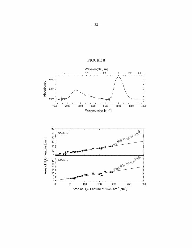
Fig. 6.— (top) Near-IR absorbance spectrum of an ∼11 µm thick H2O ice at 10 K in the range

of 7500–4000 cm−1 (1.333–2.5 µm), displaying the features at 6684 and 5040 cm−1 (1.496 and

1.984 µm); (bottom) Integrated areas (in cm−1) of H2O near-IR features plotted versus the

area (in cm−1) of the H2O feature at 1670 cm−1 (5.988 µm) during deposition at 10 K. Lines

and symbols have the same meaning as in Figure 2.

Fig. 7.— (top) Near-IR absorbance spectrum of a thick CH3OH sample at 10 K; (bottom)

Integrated areas (in cm−1) of CH3OH near-IR features plotted versus the area (in cm−1) of

– 17 –

the CH3OH feature at 2830 cm−1 (3.534 µm) during deposition at 10 K. Lines and symbols

have the same meaning as in Figure 2.

Fig. 8.— (top) Selected regions of the near-IR absorbance spectrum of a thick NH3 sample

at 10 K; (bottom) Integrated areas (in cm−1) of NH3 near-IR features plotted versus the

area (in cm−1) of the NH3 feature at 1070 cm−1 (9.346 µm) during deposition of NH3 at

10 K. Data points plotted as squares were measured from a separate deposit experiment

from those plotted with circles. Otherwise, lines and symbols have the same meaning as in

Figure 2.

– 18 –

FIGURE 1

0.0

0.5

1.0

1.5

0.0

0.5

1.0

1.5

0.0

0.5

1.0

1.5

4002000400060008000

2000400060008000100000.0

0.5

1.0

1.5

43

(magnified 20 x)

CO

2

(magnified 20 x)

CO2

(magnified 100 x)

C3O2

(magnified 5 x)

CH4

Abs

orba

nce

(magnified 50 x)

H2O

(magnified 50 x)

CH3OH

Wavenumber [cm-1]

(magnified 10 x)

NH3

25105Wavelength [ m]

1 432 105

– 19 –

FIGURE 2

4180 4170 4160 4150 4140

0.000

0.002

0.004

0.006

0.008

4220424042604280

0.0

0.4

0.8

6380 6360 6340 6320 6300

0.000

0.002

8520 8500 8480

0.000

0.005

2.40 2.412.34 2.35 2.36

1.57 1.581.172 1.176 1.18

Wavelength [ m]

Wavenumber [cm-1]

Abs

orba

nce

0.0 0.5 1.0 1.5 2.0 2.5 3.0 3.50.00

0.05

0.10

0.00

0.02

0.040

2

4

0.00

0.04

8504 cm-1

Are

a of

CO

Fea

ture

[cm

-1]

Area of 13CO Feature at 2092 cm-1 [cm-1]

6338 cm-1

4252 cm-1

4159 cm-1

– 20 –

FIGURE 3

5200 5100 5000 4900 4800

0.00

0.02

0.04

0.06

0.08

0.10

6400 6300 6200

0.0000

0.0005

0.0010

0.0015

7050 7000 6950 6900

0.000

0.002

0.004

10000 9950 9900

0.000

0.005

1.95 2.00 2.051.58 1.60 1.62

1.42 1.43 1.441.000 1.005 1.010

Wavelength [ m]

Wavenumber [cm-1]

Abs

orba

nce

0 5 10 15 20 25 30

0.0

0.1

0.2 0 5 10 15 20 25 30

0.00

0.02

0.04

0.06

0.00

0.01

0.020.000

0.005

0.010

0.0

0.2

0.4

0.6

0.0

0.5

1.0

0.0

0.1

0.2

9944 cm-1

Area of CO2 Feature at 3708 cm-1 [cm-1]

6972 cm-1

Are

a of

CO

2 Fea

ture

[cm

-1]

6341 cm-1

4971 cm-1

6214 cm-1

5087 cm-1

4832 cm-1

– 21 –

FIGURE 4

5400 5200 4600 4400 4200

0.000

0.002

0.004

1.85 1.90 1.95 2.20 2.30 2.40

Wavelength [ m]

Abs

orba

nce

Wavenumber [cm-1]

0 2 4 6 8 10 12 14 16 180.0

0.2

0.40.00

0.05

0.10

0.0

0.5

1.0

5270 cm-1

Are

a of

C3O

2 Fea

ture

[cm

-1]

Area of C3O2 Feature at 3744 cm-1 [cm-1]

4570 cm-1

4370 cm-1

– 22 –

FIGURE 5

4600 4400 4200 4000

0.0

0.5

1.0

1.5

2.0

6200 6000 5800 5600

0.0

0.1

0.2

7600 7500 7400

0.00

0.02

0.04

9200 8800 8400

0.00

0.01

0.02

0.03

2.2 2.3 2.4 2.51.65 1.70 1.75 1.80

1.32 1.33 1.34 1.351.10 1.15 1.20

Wavelength [ m]

Wavenumber [cm-1]

Abs

orba

nce

0.0

0.5

1.0

0

10

20

0

20

40

0

2

4

6

0.0

0.5

1.0

0

1

0

2

4

6

0.0

0.5

0.0

0.5

0 5 10 15 20 250.0

0.5

1.0

0 5 10 15 20 25

0.0

0.2

0 5 10 15 20 250.0

0.2

4115 cm-1

4202 cm-1

4300 cm-1

4528 cm-1

5565 cm-1

5800 cm-1

5987 cm-1

7487 cm-1

8405 cm-1

8588 cm-1

Are

a of

CH

4 Fea

ture

[cm

-1]

8780 cm-1

Area of CH4 Feature at 2815 cm-1 [cm-1]

9060 cm-1

– 23 –

FIGURE 6

7500 7000 6500 6000 5500 5000 4500 4000

0.00

0.02

0.04

1.4 1.6 1.8 2 2.2 2.4Wavelength [ m]

Abs

orba

nce

Wavenumber [cm-1]

0 50 100 150 200 250 300

051015202530

0

10

20

30

40

50

60

Are

a of

H2O

Fea

ture

[cm

-1]

6684 cm-1

Area of H2O Feature at 1670 cm-1 [cm-1]

5040 cm-1

– 24 –

FIGURE 7

410042004300440045004600

0.00

0.02

0.04

0.06

2.20 2.25 2.30 2.35 2.40

Wavelength [ m]

Abs

orba

nce

Wavenumber [cm-1]

0 2 4 6 8 10 12 14 160

1

2

3

0.0

0.2

0.4

4400 cm-1

Area

of C

H3O

H F

eatu

re [c

m-1]

Area of CH3OH Feature at 2830 cm-1 [cm-1]

4280 cm-1

– 25 –

FIGURE 8

7000 6500 6000

0.00

0.01

0.02

5500 5000 4500 4000

0.00

0.05

0.10

0.15

0.201.4 1.5 1.6 1.7 1.8 2.0 2.2 2.4 2.6

Wavelength [ m]

Abs

orba

nce

Wavenumber [cm-1]

0 50 100 150 200 250 300

0

1

2

0.0

0.5

1.0

0

20

40

0

20

40

60

6515 cm-1

Are

a of

NH

3 Fea

ture

[cm

-1]

Area of NH3 Feature at 1070 cm-1 [cm-1]

6099 cm-1

4993 cm-1

4474 cm-1