The Stochastic Discount Factor for theExponential-Utility Capital Asset Pricing

Model

Mark JohnstonPricewaterhouseCoopers,

GPO Box 2650, Sydney NSW 1171, Australiaand

University of New South Wales,Sydney NSW 2052, Australia

E-mail: mark.e.johnston@au.pwc.com

May 20, 2004

Abstract

In this paper we introduce the notion of a marginal stochastic dis-count factor for an asset. This is a function defined on the possiblepayoffs of the asset which can be used to value the asset and derivativesof it. We then show how one may derive the marginal stochastic dis-count factor for a common version of the Capital Asset Pricing Model(CAPM), namely the version derived under assumptions of exponen-tial utility and asset payoffs jointly normal with the market portfolio.The advantage of this is that it allows us to obtain equilibrium pricesfor assets which are derivatives of CAPM assets, even though thesederivatives do not satisfy the CAPM.

We then illustrate the practical application of this discount factorby showing how to value the liabilities of a firm with CAPM assets.

Our derivation of the CAPM discount factor builds upon somepapers published in the actuarial literature by Shaun Wang and HansBuhlmann.

1

1 Introduction

The capital asset pricing model (CAPM), developed in the 1960’s, is thestandard model employed today to value many assets, such as companies andprojects. The CAPM is applied as a risk-adjusted discount rate technique.The latter says that an asset with payoff xj (a random variable) can be valuedaccording to the formula:

pj =E(xj)

E(Rj).

Here pj denotes the price of the asset, and the number E(Rj) is the expectedor required return on the asset. The CAPM gives a particular formula forthe required return in terms of the relative riskiness of the asset and themarket. This formula applies only to assets which satisfy the assumptions ofthe CAPM.

Modern equilibrium asset pricing theory is cast in terms of stochasticdiscount factors. These are random variables that allow assets to be pricedaccording to formulae like:

pj = E(m xj),

where m is the stochastic discount factor (for example see [Coc01, LW01]).The single discount factor m may be used to value all traded assets. Thestochastic discount factor approach is very general, which is especially usefulfor consideration of theoretical valuation questions. To apply the approachto answer practical valuation questions, one can either estimate a discountfactor directly from data, as described in Cochrane’s book [Coc01], or employa specialisation of the approach that is reasonable for whatever particularclass of assets one is interested in.

In this paper we introduce the notion of a marginal (stochastic) discountfactor for an asset. This is a function defined on the possible payoffs of theasset which can be used to value the asset and derivatives of it. We thenshow how one may derive the marginal stochastic discount factor for a com-mon version of the CAPM, namely the version derived under assumptions ofexponential utility and asset payoffs jointly normal with the market portfo-lio. The advantage of this is that it allows us to obtain equilibrium prices forassets which are derivatives of CAPM assets, even though these derivativesdo not satisfy the CAPM.

We then illustrate the practical application of this discount factor byshowing how to value the liabilities of a firm with CAPM assets.

Our derivation of the CAPM discount factor builds upon some paperspublished in the actuarial literature by Shaun Wang and Hans Buhlmann.In his paper of 1980 [Buh80a], Hans Buhlmann developed a model for de-

2

termining “optimal risk exchanges” in a closed market. Wang [Wan03] hasrecently shown that the “Wang Transform,” originally developed in a prob-ability distortion operator approach to asset pricing [Wan02], arises also inan expected-utility equilibrium context, in a specialisation of Buhlmann’smodel. What we think is noteworthy about the Buhlmann paper is that itprovides an explicit formula for what in modern terminology is the stochasticdiscount factor, as a function of total consumption.

Here we will set out the results of Buhlmann in the more familiar frame-work of expected-utility asset pricing, and then will go on to show how Wang’stransform arises as as a way of pricing certain assets within a specialisationof the Buhlmann economy. For these assets, which we might call the Wangassets, we can exhibit an explicit formula for the marginal stochastic dis-count factor. We will then show that a subset of the Wang assets, thosewhich have normally distributed payoffs, can be priced using the capital as-set pricing model. This set of assets is closed under linear combinations, andso forms a linear subspace of the space of all assets in the Wang-Buhlmanneconomy. We exhibit an explicit form for the marginal discount factor forCAPM assets — which turns out to be exponential in the payoff of the asset.

2 Background

In this section we will introduce the stochastic discount factor approach toasset pricing, and describe the connection between this approach and therisk-neutral valuation approach. We will discuss returns and Sharpe ratios,and show how Sharpe ratios of assets may be related to the Sharpe ratio ofthe stochastic discount factor. We will set out some formulae for expectedreturns and Sharpe ratios of linear combinations of assets, which will beuseful in what follows.

2.1 Securities market equilibrium

In modern texts asset pricing texts such as LeRoy and Werner [LW01],Cochrane [Coc01] and Panjer et. al. [P+98], it is shown that at a complete-market equilibrium in a single-period expected-utility endowment economy,an asset with payoff x may be priced via the formula:

p = E(m x),

where m = mi for all i, and

mi =u′i,1(c

∗i,1)

u′i,0(c∗i,0)

(1)

3

is agent i’s marginal rate of substitution between consumption at the start ofthe period and consumption at the end of the period. At the complete mar-kets equilibrium, the agents’ marginal rates of substitution agree, and we referto m as the stochastic discount factor. Here we have supposed that agent ihas a utility function of the form (“separable”): ui(c0, c1) = ui,0(c0)+ui,1(c1),where ct represents the agent’s consumption at time t. The equilibrium formsthrough agents buying and selling securities with the aim of maximising theirexpected utility. We denote the resulting optimal consumption allocations byc∗i,0, c∗i,1. The optimal end-of-period consumption c∗i,1 is a random variable— it varies over “states of the world”. We can think of states of the worldas being elements ω of a state space Ω, and random variables as functionsfrom Ω to the real numbers R. Since c∗i,1 is a random variable, the stochasticdiscount factor m is a random variable.

At equilibrium, the securities market clears — for every buyer there is aseller. Writing θ∗i,j for the optimal amount of security j held by agent i, themarket clearing conditions are:

I∑i=1

θ∗i,j = 0,

for each security j. We will write the total end-of-period consumption asc(ω) =

∑Ii=1 c∗i,1(ω). In a single-period model, end-of-period consumption

equals end-of-period wealth [Coc01, P+98]. We may thus consider c to betotal wealth.

2.2 No-arbitrage

A set of payoffs and their corresponding prices are said to be arbitrage-freeif each positive payoff has a positive price. By positive payoff we mean apayoff that is not negative in any state, and is positive in at least one state.By strictly positive payoff we mean a payoff which is positive in all states.

This property of prices can be translated into a property of the discountfactor: A set of payoffs and prices is arbitrage-free if and only if there existsa strictly positive discount factor (see e.g. [Coc01]).

2.3 Relationship with risk-neutral pricing

Here we describe briefly the connection between pricing using stochastic dis-count factors and pricing using risk-neutral probabilities.

If we make the assumptions of no-arbitrage, and complete markets, thestochastic discount factor approach becomes the risk-neutral pricing ap-proach. This is easiest to think about in the finite-state-space context, so

4

assume Ω is a finite set, and let π(ω) denote the probability of state ω. Thenthe price of an asset that pays x(ω) in state ω is:

p = E(m x) =∑ω∈Ω

m(ω) x(ω) π(ω) = E(m)∑ω∈Ω

x(ω) πQ(ω),

where we have defined the numbers πQ(ω) as

πQ(ω) = π(ω)m(ω)

E(m). (2)

The numbers πQ(ω) add up to one, by construction, and since we have as-sumed no-arbitrage, the discount factor m is strictly positive (see e.g. [Coc01]),so the numbers πQ(ω) are non-negative. Thus we may consider them a setof probabilities, which we will call the risk-neutral probabilities, and write:

p =EQ(x)

Rf

, (3)

where we have defined Rf = 1/E(m), and EQ represents the expectation withrespect to the risk-neutral probabilities, rather than the original, “physical”,probabilities (which give the likelihoods of states of the world). The labellingof 1/E(m) as Rf follows from the fact that if a risk-free asset is traded, mean-ing an asset which pays an amount 1 in every state, then it’s price is E(m),so 1/(E(m) can be interpreted as the risk-free gross return. Equation (3)embodies the risk-neutral pricing approach: “To value an asset, calculate itsexpected payoff with respect to the risk-neutral probabilities, and discountat the risk-free rate”.

Equation (2) shows that the stochastic discount factor describes the trans-formation between physical and risk-neutral probabilities — the stochasticdiscount factor, scaled by its mean, may be thought of as the derivative ofthe risk-neutral probabilities with respect to the physical probabilities, or a“change of measure”.

2.4 Returns, and the market price of risk

By the gross return, or just return on an asset x with non-zero price, wemean the random variable Rx = x/p(x), payoff divided by price. The returnis just a scaled version of the asset. It has price 1. Any asset with price1 can be considered to be a return. The expected return is the numberE(Rx) = E(x)/p(x). This expectation is of course taken with respect to the

5

real-world probability measure. We can easily show that the expected returnof any asset in the risk-neutral measure is the risk-free return:

EQ(Rx) = EQ

(x

p(x)

)=

EQ(x)

p(x)=

EQ(x)

EQ(x)/Rf

= Rf .

In the real-world probability measure one finds, through application of thepricing formula p = E(m x) and the definition of covariance, that

E(Rx) = Rf (1− cov(m,Rx)), (4)

so that expected returns are greater/lesser than the risk-free return accordingto whether the covariance of the asset with the stochastic discount factor isnegative/positive, or equivalently (when the SDF has been derived in anequilibrium model) whether the covariance of the asset with consumption ispositive/negative.

For any asset x with non-zero price we define the Sharpe Ratio as theratio of expected excess return to standard deviation of return:

λx =E(Rx)−Rf

σRx

. (5)

This ratio is also known as the market price of risk of asset x, as it shows howmuch excess return will be demanded per unit of risk (measured as returnstandard deviation). Applying formula (4) yields:

λx =−Rf cov(m, Rx)

σRx

.

Multiplying top and bottom by p(x) gives:

λx =−Rf cov(m, x)

σx

,

where σx is the standard deviation of x. Accordingly, we have:

λx = −Rf σm ρmx,

where σm is the standard deviation of the stochastic discount factor, andρmx is the linear correlation coefficient of m and x. We can consider m as anasset, in which case

λm =−Rf cov(m, m)

σm

= −Rf σm,

6

so for any asset x we have:λx = ρmx λm. (6)

In words: the Sharpe Ratio for an asset x is the product of the Sharpe Ratioof the stochastic discount factor and the linear correlation coefficient of theasset with the discount factor. The reader may note that if m is interpreted as“the market”, equation (6) is the capital asset pricing model. We will discussthis further later. In general m does not admit such an interpretation, butthis CAPM-like formula holds.

We’ll now show how expected returns and Sharpe Ratios behave whenwe form portfolios of assets. Suppose an asset x is the sum of two assets yand z: x = y + z. Then:

p(x) Rx = p(y) Ry + p(z) Rz,

so:

Rx =p(y)

p(x)Ry +

p(z)

p(x)Rz,

and consequently the expected return of x is given by:

E(Rx) =p(y)

p(x)E(Ry) +

p(z)

p(x)E(Rz).

This is a “weighted average cost of capital” formula. The weights are therelative market values of y and z.

Using the definition of the Sharpe Ratio in terms of the mean and stan-dard deviation of the payoff of x, we see that:

σx λx = −Rf cov(m, x)

= −Rf cov(m, y + z)

= −Rf ((cov(m, y) + cov(m, z))

= σy λy + σz λz,

and hence we obtain a “weighted average price of risk” formula:

λx =σy

σx

λy +σz

σx

λz,

where the weights are the relative standard deviations of the asset payoffs.

7

3 Marginal discount factors

A stochastic discount factor is a function from Ω to R. The state space Ω isin general a high-dimensional space. Often we will want to use a stochasticdiscount factor to price a particular asset, or derivatives of a particular asset,and we’d like to graph the stochastic discount factor as a function of thepayoff of the asset. When we do this, we are actually graphing what wemight call the marginal stochastic discount factor for that asset. To makethis concrete, suppose x is an asset, m is a stochastic discount factor, and foreach s ∈ R let x−1(s) denote the set of states ω ∈ Ω : x(ω) = s (the levelset of x corresponding to the value s). Consider a derivative of x, meaning anasset with payoff of the form g(x) for some function g. We call it a derivativeof x because its payoff is determined by the payoff of x. Writing f for theprobability density function corresponding to the real-world probabilities,the value of this derivative is given by:

E(m g(x)) =

∫ω∈Ω

m(ω) g(x(ω)) f(ω) dω

=

∫s∈R

∫ω∈x−1(s)

m(ω) g(s) f(ω) dω ds

=

∫s∈R

g(s) fx(s)

(∫ω∈x−1(s)

m(ω)f(ω)

fx(s)dω

)ds

=

∫s∈R

mx(s) g(s) fx(s) ds

= E(mx g(x)),

where mx(s) is the quantity in brackets, and fx is the marginal density of x.The quantity f(ω)/fx(s) is the conditional density with respect to x. Thusmx is the conditional expectation of the SDF with respect to x.

As mx is defined in the same way as the marginal probability density of x,that is by integrating over the level sets of x, we refer to mx as the marginaldiscount factor of x. Just as the marginal density is all one needs to calculateexpectations of functions of x, so the marginal density and marginal discountfactor are all one needs to compute the values of functions (“derivatives”)of x. When we draw a graph of a discount factor it’s usually a marginaldiscount factor that we are drawing.

8

4 Derivation of Buhlmann’s model in the SDF

framework

Under the standard assumption that marginal utility is strictly positive, theend-of-period marginal utility function will have a local inverse at the optimalconsumption point, so we may invert the relationship (1) to obtain:

c∗i,1(ω) = (u′i,1)−1(u′i,0(c

∗0) mi(ω)

).

We can thus express total consumption in terms of the discount factors asfollows:

c(ω) =I∑

i=1

c∗i,1(ω) =I∑

i=1

(u′i,1)−1(u′i,0(c

∗0) mi(ω)

). (7)

To proceed further we need to assume that we can replace the mi with min this formula. As noted above, this will be possible in a complete marketssetting. To deal with the incomplete markets case we need to understandwhat happens when we take projections on each side of the above equation.The left hand side would become the traded part of consumption/wealth(call it the “market portfolio”). We will return to this matter in a subsequentpaper.

Replacing each mi with m in (7), we have:

c(ω) =I∑

i=1

(u′i,1)−1(u′i,0(c

∗0) m(ω)

). (8)

In Buhlmann’s second paper on this topic [Buh80b], he notes that in thegeneral case one can use the implicit function theorem to argue that equa-tion (8) can be solved for m in terms of c. In his first paper, he obtains anexplicit solution by assuming that agents have exponential utility functions:

ui,1(c) =1

αi

(1− e−αi c),

where αi is a parameter known as the absolute risk-aversion, in which case:

u′i,1(c) = e−αi c,

and so:

(u′i,1)−1(s) =

−1

αi

log s.

9

Under this exponential utility assumption the terms of the sum in (8) splitand we get:

c(ω) =I∑

i=1

− 1

αi

log(u′i,0(c

∗0))−

(I∑

i=1

1

αi

)log(m(ω)).

We then conclude that m is an exponential function of aggregate consumption

m(ω) = A e−α c(ω),

where α is the harmonic sum of the αi:

1

α=

I∑i=1

1

αi

,

and A is a positive constant. A formula for the constant A can be writtendown in terms of the risk-aversion coefficients and the time-zero marginalutilities, or if a risk-free asset is traded we can calibrate A by requiring thatthe expected value of the discount factor be the inverse of the risk-free return.

5 Stochastic discount factor for Wang assets

In the previous section we showed that in the Buhlmann economy we couldobtain an explicit form for the stochastic discount factor, as a function ofaggregate consumption. In this section we will place a further restriction onthe economy, namely that aggregate consumption is normally distributed,and will show that this allows us to determine marginal discount factors forcertain assets (those which are normal-copula with consumption).

Accordingly, following Wang [Wan03], assume c is normally distributed,and let z be the standard normal variable obtained from c by subtractingits mean and dividing by its standard deviation: z = (c − µc)/σc. Thenthe discount factor can be re-written as m = B e−λ z, where λ = α σc. Thestochastic discount factor thus has a log-normal distribution in this economy.

Assume an asset x is normal-copula with total consumption, meaning herethat x may be written as x = h(v), where h is an increasing function, and vand z have a standard bi-variate normal distribution with correlation coeffi-cient ρ. In this case we can decompose z in a way which allows us to directlycompute what the marginal discount factor for x. Let y = z − ρ v. Then yand v are also jointly normal, and as cov(y, v) = cov(z, v)− ρ cov(v, v) = 0,y is independent of v (for jointly-normal variables, zero covariance impliesindependence).

10

Consider a derivative of x, g(x). The value of this asset is given by:

E(m g(x)) = E(B e−λ (y+ρ v) g(h(v))

)= E

(B e−λ y e−λ ρ v g(h(v))

)Since y and v are independent, we may write this as:

E(m g(x)) = E(B e−λ y

)E(e−λ ρ v g(h(v))

)= E(mx g(x)),

say, wheremx = C e−λ ρ h−1(x),

and C is a constant. Thus we have derived a stochastic discount factor, mx,which prices any derivative of x via the one-dimensional integral:

p(g(x)) = E(mx g(x)) =

∫ ∞

−∞mx(s) g(s) fx(s) ds,

where fx is the marginal probability density of x. The function mx is themarginal discount factor for x, as per our earlier definition.

The fact that the variable v is jointly-normal with consumption meansthat all information about the dependence between v and consumption is cap-tured by a single number, the correlation coefficient. This, together with theassumption of exponential utility, has allowed us to separate the expressionE(m g(x)) into a product of two expectations, which means two integrals,one over x and one over all the other dimensions of the state space, uncondi-tional on x. This is what gives us an explicit form for the marginal discountfactor in this case.

When a risk-free asset is traded, the constant C above may be determinedby requiring that the expected value of mx be 1/Rf , in which case we findthat:

mx(s) =1

Rf

e−λ2

x2 e−λx h−1(s), (9)

where λx = λ ρ. Wang refers to the parameter λx as the market price of riskfor the asset x, and we will discuss later the reasons for this. It is really themarket price of risk of the underlying asset v.

5.1 Connection with the Wang Transform

In the remainder of the paper [Wan03], Wang goes on to show that the pricesof Wang assets may also be calculated as:

p(x) =1

Rf

EQ(x),

11

where EQ represents the expectation with respect to a transformed proba-bility distribution FQ

x , the Wang Transform of Fx, defined by

FQx (s) = Φ

(Φ−1(Fx(s)) + λx

), (10)

where Fx is the cumulative distribution function (CDF) of x and Φ is theCDF of a standard normal variable.

Note that by differentiating Equation (10) we can establish a formula forthe probability density function of the transformed variable:

fQx (s) = (FQ

x )′(s) = e−λ2

x2 fx(s) e−λx Φ−1(Fx(s)),

where fx(s) is the original probability density function: fx(s) = F ′x(s). We

may then apply Equation (2) to recover the formula (9) for the stochasticdiscount factor (where h−1(s) = Φ−1(Fx(s))).

6 Stochastic discount factor for CAPM

We have shown that in a single-period endowment economy, where agents areexpected-utility maximisers and have separable utility functions, with theend-of-period utility being exponential, and where the total end-of-periodendowment/consumption is normally distributed, we can derive an explicitexpression for the stochastic discount factor in terms of total consumption,and that for certain assets within this economy, namely those which arenormal-copula with consumption, we can derive an explicit expression forthe marginal stochastic discount factor.

The set of assets which are jointly normal with consumption are of par-ticular interest, as we shall see. For brevity we’ll call them normal assets,or CAPM assets (see below) but remember that this means more than justthat they have a normal distribution, it means they are jointly normal withconsumption. This is a stronger condition — two variables can each havenormal marginal distributions but not be jointly normal; their dependencystructure could be characterised by some other copula (see e.g. [Ven03]).

If x and y are jointly normal with consumption, then so is a x + b y forany real numbers a and b, so the space of normal assets is closed under linearcombinations, and so forms a vector subspace of the space of all assets. Thismeans that a portfolio of normal assets is a normal asset. This property doesnot hold for the Wang assets, for example.

Actually, since the marginal stochastic discount factor for an asset canbe used to price all derivatives of that asset, and since any asset which isnormal-copula with consumption is a derivative of an asset which is jointly

12

normal with consumption (x = h(v) in the above), we need only considerassets which are jointly normal with consumption to derive the benefits of theWang transform in this expected-utility setting. However, it may be moreconvenient to work with the marginal distribution and marginal discountfactor of the asset under investigation, than to work in terms of those of theunderlying normal asset.

If an asset x has payoff which is normal with mean µx and standarddeviation σx, then it may be related to a unit normal variable v via theincreasing transformation x = h(v) = µx + σx v. The inverse transformationis h−1(x) = (x − µx)/σx, so we see from (9) that the marginal stochasticdiscount factor for x is:

mx(s) =1

Rf

e−λ2

x2 e−λx (s−µx)/σx , (11)

so the marginal stochastic discount factor for a normal asset is exponentialin the payoff of the asset.

6.1 Relationship with traditional CAPM

The reader may recall that assumptions of exponential utility and asset pay-offs jointly normal with consumption give one way of deriving the CapitalAsset Pricing Model (CAPM) (see e.g. [Coc01]). Normally one arrives atthe CAPM by assuming that all assets have payoffs jointly normal with con-sumption, and proceeding by pricing assets relative to the “market portfolio”consisting of all assets in the economy. Here we have taken a slightly differentapproach, and allowed in the securities market assets which have non-normalpayoffs. What we have shown is that we can obtain a stochastic discountfactor that prices the normal assets, and derivatives of them. We can thusprice a broader set of assets, using the normal assets as a base, and employ-ing the two tools at our disposal, namely the ability to price derivatives ofnormal assets, and the ability to price portfolios of assets, which follows fromthe linearity of the pricing operator.

We have yet to show that our marginal discount factors applied to thenormal assets produce the CAPM. We’ll see this below.

6.2 Properties of the CAPM discount factor

Suppose x is a derivative of a normal asset v: x = h(v). Without loss ofgenerality we can assume v is unit normal (a derivative of a normal asset isalso a derivative of a unit normal asset). Then we may value x using the

13

marginal discount factor of v as follows:

p(x) = E(mv h(v))

=

∫ ∞

−∞mv(s) h(s) fv(s) ds

=

∫ ∞

−∞

1

Rf

h(s) e−λ2

v2 e−λv s e

−s2

21√2 π

ds

=

∫ ∞

−∞

1

Rf

h(s)e−

(s+λv)2

2

√2 π

ds

=

∫ ∞

−∞

1

Rf

h(s− λv)e−s2

2

√2 π

ds

=1

Rf

E(h(v − λv))

This is a convenient formula for pricing normal assets and their deriva-tives. We’ll consider a couple of examples below. Note that the λ used isthat of v, i.e. λv = ρvc λ.

Value of a normal asset Let x be a normal asset with mean µ andstandard deviation σ. Then x is a derivative of a unit normal asset v viax = h(v) = µ + σ v, so the price of x is:

p(x) =1

Rf

E(µ + σ (v − λv)) =1

Rf

((µ− λv σ) + σ E(v)) =1

Rf

(µ− λv σ).

As x is a linear function of v, it has the same correlation with total consump-tion, so λv = ρvc λ = ρxc λ = λx.

Value of an asset whose log is normal Let x = h(v) = eµ+σ v, where vis a unit normal asset. Then the price of x is:

p(x) =1

Rf

E(eµ+σ (v−λv)) =1

Rf

eµ−λv σ E (eσ v) =1

Rf

eµ−λv σ+σ2/2.

Value of a call option on a normal asset Let x = max(0, y−K), wherey is a normal asset: y = µ + σ v. Then x = max(0, µ + σ v−K), so the priceof x is:

p(x) =1

Rf

E (max(0, µ−K + σ (v − λv))) =σ

Rf

E(max(0, a + v)),

14

where a = (µ− λv σ −K)/σ = (Rf p(y)−K)/σ, so

p(x) =σ

Rf

∫ ∞

−a

(a + s) φ(s) ds =σ

Rf

(a Φ(a) + φ(a)) , (12)

where φ and Φ are respectively the probability density function and cumu-lative distribution function of a standard normal variable.

6.3 Risk-neutral probabilities for CAPM assets

Applying the definition of risk-neutral probabilities (2), and the form of themarginal SDF for CAPM assets (11) we see that the risk-neutral probabilitydistribution for a normal asset x is just the physical distribution shifted tothe left by a distance λx σx:

fQx (s) = fx(s + λx σx).

Wang [Wan02] derives this result using the Wang transform.

6.4 Showing that normal assets satisfy the CAPM

We have been referring to the normal assets as CAPM assets, but we haven’tyet shown that they satisfy the CAPM. We’ll do that here.

Suppose x is a normal asset with parameters µx, σx, λx. Then the re-turn on x is also a normal asset, with mean E(Rx) = µx/p(x) and standarddeviation σRx = σx/p(x). Recall that for a normal asset,

p(x) =1

Rf

(µx − λx σx).

Solving this for λx we get:

λx =µx −Rf p(x)

σx

=E(Rx)−Rf

σRx

.

Comparing this to equation (5), we see that for normal assets the SDF pa-rameter λx is the Sharpe Ratio of the asset x (which is why we denoted itby λx and have been referring to it as the market price of risk of asset x).

Recall that in the Wang-Buhlmann economy total consumption, c, isnormal, and has λc = λ, so applying the above formula to total consumptionyields:

λ =E(Rc)−Rf

σRc

.

15

We may thus interpret λ as the Sharpe Ratio of consumption, and refer toit as the market price of risk.

Recalling that the market price of risk of a normal asset x is related tothe overall market price of risk via λx = ρxc λ, where ρxc is the correlationcoefficient of x and c, we see that:

E(Rx)−Rf

σRx

= ρxcE(Rc)−Rf

σRc

,

and we may re-write this as:

E(Rx) = Rf + βx (E(Rc)−Rf ) ,

whereβx = ρxc

σRx

σRc

.

This is the capital asset pricing model (see e.g. [P+98]). As pointed outearlier, in a single-period model total end-of-period consumption equals totalend-of-period wealth, so the return on consumption Rc may be thought ofas the return on wealth, or the return on “the wealth portfolio”, which ishow the CAPM is usually presented. If markets are complete (as we haveassumed in deriving the Wang-Buhlmann model), then the wealth portfoliocan be represented by a particular combination of traded securities, whichwe might call “the market portfolio”. From the relationship λx = ρxc λ, andthe fact the correlation coefficients are no larger than one in absolute value,we conclude that normal assets can have a Sharpe ratio no greater than thatof the market portfolio — so the market portfolio is efficient among normalassets in the sense that it offers the greatest ratio of excess return to risk.

7 Example — a limited-liability firm

Here we will introduce a simple model of a limited-liability firm, followingSherris [She04] and Johnston [Joh03], and illustrate how the discount factorsdeveloped above can be applied to value the components of the firm’s balancesheet. The discount factors developed above are useful in this context, asbalance sheet components are sums of other balance sheet components, so ifwe assume certain components (e.g. the assets and the claims) are normal,others (e.g. the surplus) will be also. We first introduce the model withoutany distributional assumptions, and in the subsequent section we considerthe case of a normal surplus.

Suppose the firm exists from time 0 to time T . The assets of the firm payAT at time T (a random variable), and have value A0 at time 0. Suppose the

16

firm has creditors, being providers of finance or trade creditors for example,who have been promised, and will claim, an amount CT at time T . Sincethe firm operates under limited liability, the amount that the creditors willactually receive at time T , which we’ll call the liability payoff, denoted byLT , is the lesser of their claim and the available assets:

LT = min(CT , AT ).

Note that if AT can take negative values, then creditors may receive a neg-ative payoff at time T . In reality creditors will not pay money into thecompany in the event of default, but these negative payoffs correspond withsituations where the company not only has no assets but has unfunded obliga-tions, for example unfunded employee entitlements, or unfunded environmen-tal clean-up obligations, and those owed will have to meet these obligationsfrom their own pockets, for example the local government may have to un-dertake environmental remediation work that the company should have paidfor.

Let DT = CT − LT be the deficit between what creditors were promisedand what they will be paid. Then:

DT = max(CT − AT , 0), (13)

and LT = CT − DT . As for the assets, we’ll let the subscript zero denotevalue at time 0 — so for each balance sheet component X we have X0 =EQ(XT )/Rf , or equivalently X0 = E(m XT ). By the linearity of the pricingoperator we have: L0 = C0 − D0 — “the value of the liabilities equals thevalue of claims less the value of the deficit”. Sherris [She04] describes D0 asthe value of the insolvency exchange option, as it is the value that accrues toshareholders from the fact that at time T they have the option to exchangethe assets for the claims.

Any money remaining after creditors have been paid will accrue to theowners of the firm — the equity providers. The cash flow to equity is thus:

ET = AT − LT = AT −min(CT , AT ) = max(AT − CT , 0).

Also,ET = AT − (CT −DT ) = (AT − CT ) + DT = ST + DT ,

where we denote the difference between the asset payoff and the claims byST , the surplus. Accordingly, E0 = S0 + D0: “equity value is the value ofassets less the value of creditors’ claims, plus the value of the insolvencyexchange option”.

The balance sheet of the company, at market values, thus looks like thatshown in Table 1.

17

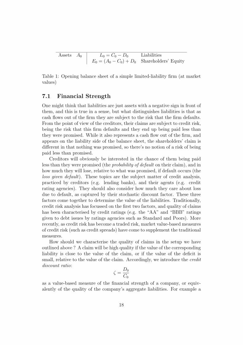
Assets A0 L0 = C0 −D0 LiabilitiesE0 = (A0 − C0) + D0 Shareholders’ Equity

Table 1: Opening balance sheet of a simple limited-liability firm (at marketvalues)

7.1 Financial Strength

One might think that liabilities are just assets with a negative sign in front ofthem, and this is true in a sense, but what distinguishes liabilities is that ascash flows out of the firm they are subject to the risk that the firm defaults.From the point of view of the creditors, their claims are subject to credit risk,being the risk that this firm defaults and they end up being paid less thanthey were promised. While it also represents a cash flow out of the firm, andappears on the liability side of the balance sheet, the shareholders’ claim isdifferent in that nothing was promised, so there’s no notion of a risk of beingpaid less than promised.

Creditors will obviously be interested in the chance of them being paidless than they were promised (the probability of default on their claim), and inhow much they will lose, relative to what was promised, if default occurs (theloss given default). These topics are the subject matter of credit analysis,practiced by creditors (e.g. lending banks), and their agents (e.g. creditrating agencies). They should also consider how much they care about lossdue to default, as captured by their stochastic discount factor. These threefactors come together to determine the value of the liabilities. Traditionally,credit risk analysis has focussed on the first two factors, and quality of claimshas been characterised by credit ratings (e.g. the “AA” and “BBB” ratingsgiven to debt issues by ratings agencies such as Standard and Poors). Morerecently, as credit risk has become a traded risk, market value-based measuresof credit risk (such as credit spreads) have come to supplement the traditionalmeasures.

How should we characterise the quality of claims in the setup we haveoutlined above ? A claim will be high quality if the value of the correspondingliability is close to the value of the claim, or if the value of the deficit issmall, relative to the value of the claim. Accordingly, we introduce the creditdiscount ratio:

ζ =D0

C0

as a value-based measure of the financial strength of a company, or equiv-alently of the quality of the company’s aggregate liabilities. For example a

18

ratio of 0.05 means that creditors will apply a discount of 5% to the value ofthe amount they were promised by the firm. Small ζ corresponds with highfinancial strength — a “strong balance sheet” (strong in a value-based sense— conveivably a firm could have low ζ by having a relatively high expectedloss, but where the loss tended to occur in high-consumption states).

Can we relate ζ to a traditional measure of credit-worthiness, such ascredit spread ? To indicate how this could be done, consider a simple casewhere the liabilities consist of a single zero-coupon bond, meaning a promiseto pay a fixed amount CT at time T (so CT is the “face value” of the bond).For a zero-coupon bond of maturity T , face value CT and market value L0,the credit spread is the number c satisfying:

L0 = e−(rf+c) T CT ,

where rf is the continuously-compounding risk-free rate for maturity T (Rf =erf T ). Solving for the spread gives:

c =1

Tln

(e−rf T CT

L0

).

Now if the bond was not subject to the default risk of the firm, its valuewould be: e−rf T CT , so in our notation, the value of the claim is:

C0 = e−rf T CT .

Accordingly,

c =1

Tln

(C0

L0

),

so the relationship between credit spread and credit discount ratio is:

c =−1

Tln(1− ζ).

Conversely,ζ = 1− e−c T .

The relationship between credit spread and credit discount given here isactually for all the claims on the firm, rather than just a debt claim. Thereason we make a distinction is that the assets of the firm might have thepossibility of negative payoff (e.g. if they are normally distributed), whiledebt claims are typically bounded below at zero — the worst outcome forthe debt providers is that they get none of their money back. Accordingly,a debt- and equity-financed firm with assets that can have negative payoffs

19

will have a residual claim, to the negative part of the asset payoff, whichis implicitly borne by employees or other stakeholders. We’ll address thepricing of the debt claim alone in a subsequent paper.

If the liabilities of a firm did indeed consist of a single zero-coupon bondthen we could just use the traditional measures such as credit spread to char-acterise the financial strength of the firm. However, the above framework setsout a measure of financial strength which applies to liabilities other than debt(for example insurance claims, environmental rehabilitation obligations), andrelates it to the measures applied to debt. The credit spread is expressed asa per-annum measure — the extra return that investors demand per annumfor taking on the firm’s credit risk — while the credit discount ratio is ex-pressed as a discount to value. Whether a per-annum measure or an absolutemeasure is better depends upon the circumstances, and upon whether onebelieves that a risk compounds over time or not. The credit spread needs tobe expressed together with a maturity in order for the value of the liabilitiesto be calculated from those of the claims.

8 Example — a firm with normal surplus

In this section we will illustrate the use of the stochastic discount factordeveloped above for normal assets, by applying it to compute the defaultdiscount for a firm with normal surplus. One example of a firm with anormal surplus is a firm with normal assets and known claims. Another isa firm with normal assets and normal claims. Accordingly, let us assumewe are in the Wang-Buhlmann economy and that the surplus of the firmis normal, in the sense introduced above. The surplus is then described bythree parameters: the mean and standard deviation of its payoff, µS and σS,and a market price of risk (Sharpe Ratio), λS. If we know the overall marketprice of risk, λ, and the correlation between ST and consumption, ρSc, thenwe can compute the market price of risk for the assets as λS = ρSc λ. Thevalue of the surplus is:

S0 = (µS − λS σS)/Rf .

As captured by Equation (13), the default deficit DT is a strike-zero calloption on the negative of the surplus, −ST = CT − AT . In the present casethe negative of the surplus is a normal asset with mean −µS and standarddeviation σS, and Sharpe Ratio −λS. Therefore the value of the defaultdeficit can be computed from the formula (12), to obtain:

D0 =σS

Rf

(a Φ(a) + φ(a)) ,

20

where

a =−µS + λS σS − 0

σS

=−S0 Rf

σS

.

The credit discount ratio is then:

ζ =D0

C0

=σS

Rf C0

φ

(−S0 Rf

σS

)− S0

C0

Φ

(−S0 Rf

σS

).

To investigate the behaviour of ζ, make the substitutions:

µ′ =S0

C0

,

σ′ =σS

Rf C0

,

δ =µ′

σ′=

S0 Rf

σS

.

Here we are expressing the surplus value as a multiple of the value of theclaims, and also dividing the standard deviation of the surplus payoff by Rf tomake it a present value and thus comparable to the other quantities (S0 andσS/Rf are the mean and standard deviation of the random variable m ST ).The quantity δ is a “distance to default,” being the number of standarddeviations (of m ST ) by which the value of the surplus (being the meanof m ST ) exceeds zero. We then have expressions for ζ in terms of thesestandardised quantities:

ζ = σ′ φ

(µ′

σ′

)− µ′

(1− Φ

(µ′

σ′

)),

= σ′ (φ(δ)− δ (1− Φ(δ))) .

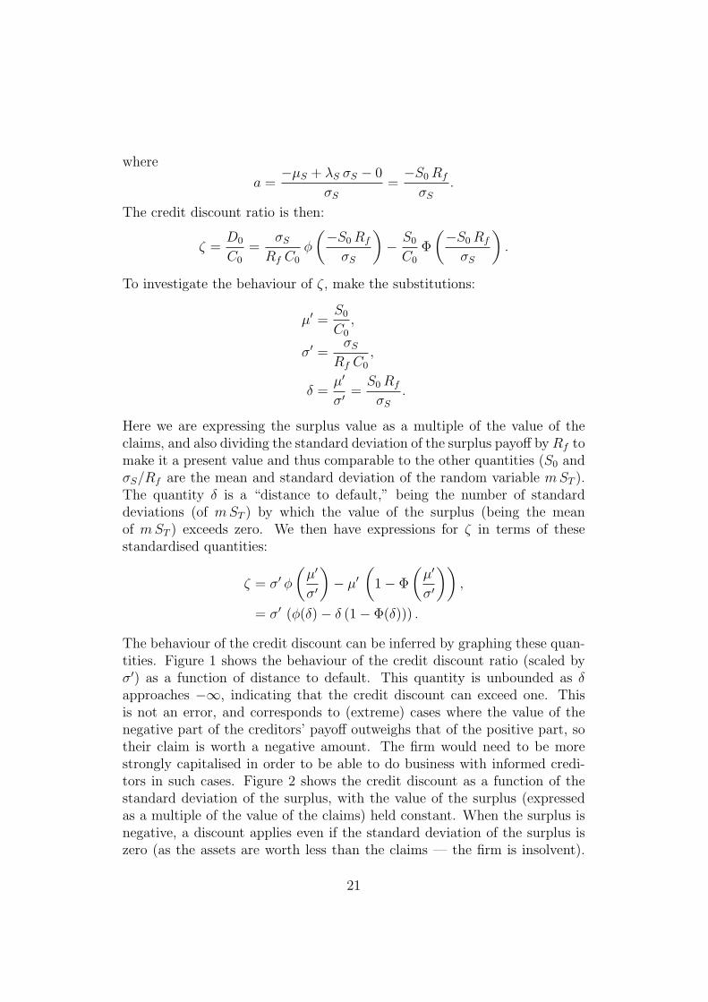
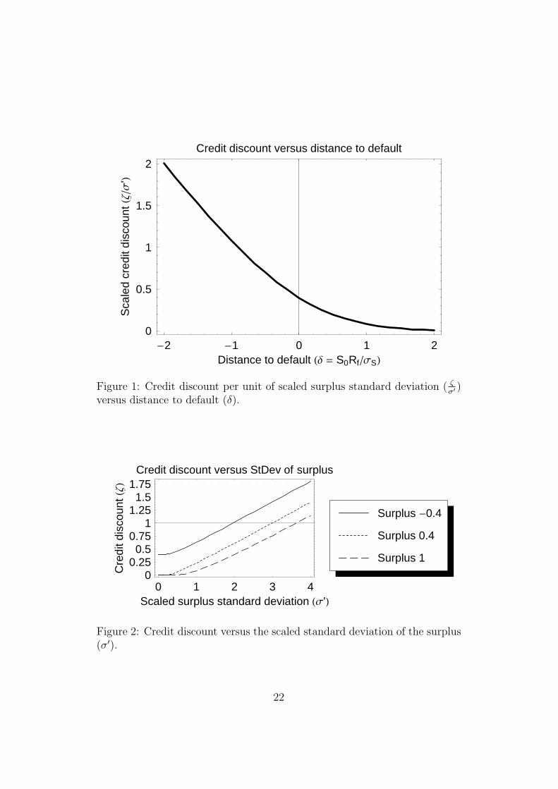
The behaviour of the credit discount can be inferred by graphing these quan-tities. Figure 1 shows the behaviour of the credit discount ratio (scaled byσ′) as a function of distance to default. This quantity is unbounded as δapproaches −∞, indicating that the credit discount can exceed one. Thisis not an error, and corresponds to (extreme) cases where the value of thenegative part of the creditors’ payoff outweighs that of the positive part, sotheir claim is worth a negative amount. The firm would need to be morestrongly capitalised in order to be able to do business with informed credi-tors in such cases. Figure 2 shows the credit discount as a function of thestandard deviation of the surplus, with the value of the surplus (expressedas a multiple of the value of the claims) held constant. When the surplus isnegative, a discount applies even if the standard deviation of the surplus iszero (as the assets are worth less than the claims — the firm is insolvent).

21

-2 -1 0 1 2Distance to default H∆ = S0RfΣSL

0

0.5

1

1.5

2

Sca

led

cred

itdi

scou

ntHΖΣ

'L

Credit discount versus distance to default

Figure 1: Credit discount per unit of scaled surplus standard deviation ( ζσ′

)versus distance to default (δ).

0 1 2 3 4Scaled surplus standard deviation HΣ'L

00.25

0.50.75

11.25

1.51.75

Cre

ditd

isco

untHΖL

Credit discount versus StDev of surplus

Surplus 1

Surplus 0.4

Surplus -0.4

Figure 2: Credit discount versus the scaled standard deviation of the surplus(σ′).

22

For each curve we can see the point where the credit discount first exceedsone, so that the claims, in aggregate, become worthless. The more realisticparts of the curves are those where the credit discount ratio is small.

9 Conclusions

We have introduced the notion of a marginal stochastic discount factor, andshown how one may derive the marginal stochastic discount factor for theexponential-utility capital asset pricing model. The advantage of this for-mulation of the CAPM is that it allows us to obtain equilibrium prices forassets which are derivatives of CAPM assets, even though these derivativesdo not satisfy the CAPM. We have illustrated the practical application ofthis discount factor by showing how the value of the liabilities of a firm witha normal surplus may be computed. In a subsequent paper we will expandupon this example to value the balance sheet components of archetypal firms— debt- and equity-funded corporations, insurance companies and banks —and examine the properties of risk-based capital allocation schemes in suchfirms.

We have arrived at the stochastic discount factor for the CAPM by set-ting out the work of Buhlmann and Wang in the stochastic discount factorframework. In the complete-markets Buhlmann economy, where agents haveexponential utility functions, the stochastic discount factor is an exponentialfunction of aggregate consumption. The stochastic discount factor is thusstrictly positive, so this economy is arbitrage-free. In the Wang-Buhlmanneconomy, which is a specialisation of the Buhlmann economy where aggregateconsumption is normally distributed, the stochastic discount factor is thuslog-normally distributed. Within the Wang-Buhlmann economy, we haveidentified two classes of assets for which we can obtain an explicit form forthe marginal discount factor. The Wang assets are those which are normal-copula with consumption. The normal assets are a subset of the Wang assets,being those which are jointly-normal with consumption. These assets forma vector subspace of the space of all assets. They satisfy the Capital AssetPricing Model (CAPM).

References

[Buh80a] Hans Buhlmann. An economic premium principle. ASTIN Bul-letin, 11:52–60, 1980.

23

[Buh80b] Hans Buhlmann. The general economic premium principle. ASTINBulletin, 14(1):13–21, 1980.

[Coc01] John H. Cochrane. Asset Pricing. Princeton University Press,Princeton, New Jersey, 2001.

[Joh03] Mark E. Johnston. Re-visiting the principles of insurance pric-ing using modern economic valuation methods. Submitted to theJournal of the Institute of Actuaries of Australia, 2003.

[LW01] Stephen F. LeRoy and Jan Werner. Principles of Financial Eco-nomics. Cambridge University Press, Cambridge, United King-dom, 2001.

[P+98] Harry H. Panjer et al. Financial Economics: with applications toinvestments, insurance and pensions. The Actuarial Foundation,Schaumburg, Illinois, USA, 1998.

[She04] Michael Sherris. Solvency, capital allocation and fair rate of returnin insurance. Preprint, University of New South Wales, 2004.

[Ven03] Gary G. Venter. Tails of copulas. Casualty Actuarial Society, 2003.

[Wan02] Shaun S. Wang. A universal framework for pricing financial andinsurance risks. ASTIN Bulletin, 32(2):213–234, 2002.

[Wan03] Shaun S. Wang. Equilibrium pricing transforms: New results usingBuhlmann’s 1980 economic model. To appear in ASTIN Bulletin,2003.

24