SUL "Z, DNA 3964F-21-1

THE ROSCOE MANUALVolume 21-1: Optics Model

Joel Garbarino

John ee Ise

General Research Corporation

P.O. Box 6770 VSanta Barbara, California 93111

c:Z 1 January 1980

Final Report for Period 9 November 1977-1 January 1980

CONTRACT No. DNA 001-78-C-0002

APPROVED FOR PUBLIC RELEASE;j'DISTRIBUTION UNLIMITED. -

M; IAR 2 5 1l ;i

ATHIS WORK SPONSORED BY THE DEFENSE NUCLEAR AGENCYUNDER RDT&E RMSS CODE B3220"78464 S990AXHC30101 H2590D.

Prepared for

Director

DEFENSE NUCLEAR AGENCY

Washington, D. C. 20305

81 3 25 065

- |-f|

-i

Destroy this report when it is no longerneeded. Do not return to sender.

PLEASE NOTIFY THE DEFENSE NUCLEAR AGENCY,ATTN: STTI, WASHINGTON, D.C. 20305, IFYOUR ADDRESS IS INCORRECT, IF YOU WISH TOBE DELETED FROM THE DISTRIBUTION LIST, ORIF THE ADDRESSEE IS NO LONGER EMPLOYED BYYOUR ORGANIZATION.

- 9N

4 _e,

_ _ _ _ _ _ _ _ _ _ _ - ~5

UNCLASSIFIED

SECURITY CLASSItICATIO4 OF T.IS PAGE 'Uhin 11m,. I ,lh.,l

j )EPRTDOUMENTATION PAGE UEO1

jOVT ACCESSION No 3 RECIPIENT'S CATA.., -kiMBER

DN TITLE1l V P-i~ TYPE OF REPORT 6 PERIOD ZOVEJ Ir.

~~Fi 1E~ N epCj *6 P-riodE RP UQ -11hNUL a 919 Nov 77-1 JLn

-#0u ez -I Optics Model tieFOMNIOGRPO

______________________________________ CR1520, vol. 21-i"U7A .os,8 CONTRACT OR GRANT NUMfLR I)

4 Joel/Garbarino -- j )DNAP- 78-C ' 02fJohn/Ise

PERFORMINmG ORGANIZATION NAME AND ADRS 0 PROGRAM CLEMLNT PROJECT TA ,.. k AREA A WORK UN:T NJMBPIG

General Research Co-poration VP. 0. Box 6770 11 u task S99QX 01 O-01

Santa Barbara, California 93111

It CONTROLLING OFFICE NAME AND ADDRESS IZ-REPORT-DATfE-

Director // 1 Jan 8tDefense Nuclear Agency IWashington, D.C. 20305 98

14 UD-NITORiNG AGENCY NAMAE 6 AOORESS0g dIleren 1o0M LC.nrroll1n4 0fl,1-e 15 SECURITYCASroh

~4'~ ~ 'UNCLASSIFIED0-~ ~ ~ I. O64 - ECLASSIFICATIONs DOV.GRAC010~--~ JSCR4EOULE

t6 DISTRIBUTION STATEMENT (of tht. Report)

Approved for public release; distribution unlimited.

17 DISTRIBUTION STATEMENT (of the Abst-Ct entered in Block 20. it differenti from Report)j

10 SUPPLEMENTARY NOTES

This work sponsored by the Defense Nuclear Agency under RDT&E RNISS CodeB322078464 S99QAJDHC30101 H2590D.

1 9 KEY WORDS (Cisrfnue an reverse side i1 necessary and ,drrfr24 by block numnb")~

Nuclear Effects SimulationOptics Ballistic Missile Defense

Computer Program

20 ABSTRACT tCoriltnue an reverse 1-dr it necess.ry and identify hv b.ock numhb-'

The ROSQE computer code is designed specifically to be the, Laboratorystandar1 -)Ifor evaluating nuclear effects on radar and optical sensors.This paper presents (1) a description of the optical code interfaceIstructure; and (2) a review of the major tasks performed by GRC--the

modeling of inhomogeneous regions. The first part describes the opticscode structure and the system simulation methodology, and,?resents some

DD 1473 EDITION OF I NOV 15 IS OBSOLETE UNCLASSIFIED kQL75$L

SECURIT CLSIIAINOFT AEi

UNCLASSIFIEDSECUAITY CLASSIFICATION OF THIS PAGEf0lhn Per& F tieed)

20. ABSTRACT (Continued)

nuclear debris, whose characterization is in terms of an expontentialautocorrelation function for integrated radiance. Separate exponentiationdecorrelation lengths are used along and perpendicular to the earth'smagnetic field, and time decorrelation is also exponehtial.

"- r

EEL

i--

" SEUNI C.A ~t"CATIN rF T|.€ PA[,'XlenO~lA Vlf¢reI

iI

sr

TABLE OF CONTENTS

Section Page

LIST OF ILLUSTRATIONS 2

INTRODUCTION 3

SUMMARY OF CODE DEVELOPMENT 42.1 Optics Code Structure 42.2 Systems Simulation Methodology and Sample 8

Output

3 MODELING OF INHOMOGENEOUS REGIONS 373.1 Introduction 373.2 G~neration of Radiant Intensities in the 39

Ideal Focal Plane

3.3 Differentiability of First-Order Markov Processes 483.4 Autocorrelation Function for Gaussian 54

Striations

REFERENCES 60

APPENDIX A: EXTRAPOLATION AND INTERPOLATION OF 61RANDOM SEQUENCE

APPENDIX B: FLOW DIAGRAMS 65

O

11

" • nn nu n

IILIST OF ILLUSTRATIONS

Figure Page

1 Systems Function Interaction Chart 5

2 Physics Function Interaction Chart 6

3 Surveillance Sensor Dynamics (OLOOK) 9

4 Object Dynamics (OPROP) 10

5 Object Charact.orization 12

6 Number of Paths/Object 13

7 Example Sight Paths for Fireball 14

8 Path Integration (SPCALC) 16

9 Example Cell List 18

10 Focal Plane Generation (OPSIM) 21

11 Variation in Mean Intensity 23

12 Spatial Correlation 2513 Time Correlation 26

14 Time Correlation 27 1

15 Multiple Fireballs 28 -

16 Multiple Objects 30

17 Multiple Objects--Growth With Time 31

18 Sensor Scan 32

19 Optics Dzta Processing 33

20 Surveillance Sensor Example 35

21 Surveillance Sensor--Example Output 36 -

22 Extrapolation of Gaussian Sequence in Three Dimensions 461

23 "Derivative" of First-Order Markov Sequence 51

24 Autocorrelation Function For Distribution of Gaussian 59

Striations

2

1 INTRODUCTION

As part of a continuing effort to supply the user community with

the best phenomenology codes available for the evaluation of nuclear ef-

fects on sensors, DNA has undertaken the task of expanding the ROSCOE

(Radar and Optical Systems Code with Nuclear Effects) computer program

to include an optical/SWIR capability.

An initial program planning phase was initiated in 1976 to formu-

late the objectives of this model, place bounds on the scope and level

of detail required, and suggest a plan for its development. The plan

called for code development during 1977 and 1978, with a completion date

of approximately January 1979, followed by a code validation and documen-

tation effort.

General Research Corporation, as part of a team of contractors, has

participated in this program development effort. GRC's responsibilities

have been primarily concerned with the development of the optics system

model and the interfacing of the optics package (both systems and physics)

with the code as a whole.

This paper presents a summary of the optics code structure. In

Section 2, a description of the optical code interface structure is given;

Section 3 presents a review of one of the major tasks performed by GRC--

the modeling of ifnhomogeneous regions. Appendix A provides some analyti-

cal backup material for Section 3, and Appendix B contains flow diagrams

for the major programs and subroutines which comprise the optics code

interface structure.

32

3N

2 SUMMARY OF CODE DEVELOPMENT

The following sections describe the optics code structure, the

system simulation methodology, and some sample outputs.

2.1 OPTICS CODE STRUCTURE

The ROSCOE code is divided into a number of separate computational

blocks which perform various parts of the systems or physics simulation.

Each block is made up of a number of subroutines, and is stored in a

separate overlay. These blocks are referred to as "events." In the

execution of the code, a series of computations, or events, is set up.

Each of these events is given a calculation time, and they are processed

(i.e., the proper overlay is called and executed) in a time-ordered

fashion. An initial list of events is set up in the input deck by the

user. Additional events may be added to the list as computations are

carried out to complete the simulation specified.

A block diagram showing the major computational blocks and infor-

mation flow for the optics code is shown in Figs. 1 and 2. The optics

systems blocks, or events, are shown in Fig. 1, and the physics events

in Fig. 2. Some interface blocks whic.. feed phenomenology data to the

systems blocks are shown in both figures.

The physics portion of the model (Fig. 2) is comprised of a burst

event which creates the initial burst parameters and several update

events to update the nuclear environment in time. In the low-altitude

region (<90 km), an update event is used to maintain the fireball and

debris region data at two times. The update event calls the fireball

and debris model routines at specified times to update these data, and

then they are interpolated at intermediate times as requested for systems

calculations or for printout.

A similar diagram for the ROSCOE radar code is given in Volume 1 of The

ROSCOE Manual.

4

- --

• .OI "* - " - rt a'

-,- .4Z4I I --

---- -- =-3 .i3i

0.__ .. - o - - -- °= a ~< .6.. . .. t3'1 ' i _ .. O 3.33

',3 . ..3,I L,,=<!I I ,

'!' * 3;

,o ., _" 1:.- _a

a -]

-__

- -

FIT-

9 5

, --°'.. r.

,, 5 t ,

In - ! 0

e .. .- -< " " ' , . = 4

0 XIM

I- - I-~

z-1 a Erlf

i - "" .J a. - '--

L - - - -I

I-I

I- ,,n I 1" t-

9.'-" - '--a.O0.I,,- , -.AL__ a'

-- -'-

The high-altitude data are also maintained at two times. Here,

because the nuclear effects may be more widespread, a grid of physical

data (chemistry, striations) is computed in addition to fireball and

debris properties (which are treated as overlays on the grid).

The optics system portion of the code consists of (1) an attack

generation event, which initializes the ambient atmosphere and magnetic

field models and creates objects to be viewed by the sensor; (2) an

optics look event (OLOOK), which sets up the sensor look geometry; 13)

an optics propagaticn path event (OPROP), which sets up the number and

position of sight paths in the sensor field of view for creating the

"scene" at the focal plane; (4) a sight path calculation event (SPCALC),which performs the integration of the radiation transport equation along

each sight path; (5) a simulated eptics event (OPSIM), which generates a

focal plane array using the sight path data and nimulates the scanning

and signal processing functions of the optical sensor; and (6) a set of

system events (currently there is only an optical track function (OTRACK)

modeled here) to simulate various system functions such as track, homing,

or discrimination.

The systems/physics interface structure is much the same as for the

radar code. The propagation and sight path calculation events access

phenomenology region data (e.g., fireball, debris, dust, beta tube para-

meters) by calling a subroutine which interpolates these data in time.

= The sight path calculation event also accesses a point properties module.

It supplies the time and location of the point in space, and the point

properties mcdule returns the appropriate data requested. These data

include temperature, mass density, chemical composition, cloud statistics,

striation statistics, earth albedo, prompt and delayed ionization, and

particulate optical properties. In addition, the sight path calculator

accesses preprocessed band emission data from external data blocks. |

7

2.2 SYSTEMS SIMUIATION METHODCLOGY AND StMPLE OUTPUT

This section describes the optical system simulation methodology.

The discussion which follows describes the use of the SWIR code by guid-

ing the reader through the simulation procedure block by block, and

displaying some intermediate code outputs.

1. Surveillance Sensor Dynamics (OLOOK). An example of how

the optics look (OLOOK) event sets up the look geometry for a surveillance-

type sensor is illustrated in Fig. 3. The boresight of the sensor is

determined from the sacellite position and a reference position, as shown.

The frame time (the time it takes for the sensor to complete its circular

scan) is input, and must be consistent with the scan rate desired.

Scanning motion is simulated by creating a frozen frame of the

environment at a selected engagement time and then sweeping over this

frame in a circular fashion at the appropriate rate.

2. Object Dynamics (OPROP). In the optics propagation (OPROP)

event, the object motion in the sensor field of view is treated by inter-

polating in time for the position of each object, and then transforming

these coordinates to the sensor coordinate frame. Objects treated include

nuclear bursts and their associated ionization regions, booster plumes, and

natural clouds (see Fig. 4).

The sensor coordinate frame* is defined by setting the z-vector

anti-parallel to the boresight. The y-vectcr is in the plane formed by

the z-vector and the satellite position vector, and is directed as close

to the satellite position vector as possible. The x-vector is chosen to

complete the right-hand system.N *ThThe block names are given here so that the radar can refer back to the

block diagrams shown in Figs. 1 and 2.

This coordinate system is used in generating the focal plane array.

'p IL

REFERENCE POSITION -- --- "" " SATELLITE

--- POSITION

/SCAN BY SENSORI TATION

o BORESIGHT ESTABLISHED BY POINTING AT REFERENCE POSITION

* FRAME TIME BASED ON ROTATION RATE

* CIRCULAR SCAN SIMULATES SENSOR MOTION

Figure 3. Surveillance Sensor Dynamics (OLOOK)

9gL

SENSORCOORDINATE COFRAME

y2

x

- -~#-#- SENSOR

POSITION- - -- -- VECTOR

*OBJECTS INCLUDE - NUCLEAR BURSTS (ASSOCIATED REGIONS)

- BOOSTER PLUMES

-NATURAL CLOUDS

*SENSOR COORDINATE FRAME

Figure 4. Object Dynamics (OPROP)

10

3. Object Characterization (OPROP). To characterize the objects

in the focal plane of the sensor, the code integrates the radiation trans-

port along a number of paths from the sensor which intersect each object.

Since these path integraticns can be time-consuming, an attempt is made to

minimize the number of paths used by selecting a relatively few paths and

interpolating between them later to generate finer detail in the focal

plane.

Objects or regions are divided into three types: (1) point objects,

which are objects whose dimensions are small compared to the sensor reso-

lution; (2) extended objects (such as fireballs), which may be bright and

cover many resolution cells; and (3) background, or other regions which __

are less bright or very extensive (cover the entire field of view).

Point objects can be characterized by a single path, as shown in

Fig. 5. Extended objects are treated by taking the object projection in

a plane normal to the vector between the sensor and the object, and select-

ing a set of points within this boundary. Finally, the background is

treated in as much (or as little) detail as the user feels is warranted

by setting up a grid of points within the sensor field of view. The user

selects the grid spacing in the Lnput deck. A default value of four points

is used as a minimum.

4. Number of Paths/Object (OPROP). The number of paths used to

characterize an extended object is a function of the object size and the

sensor resolution, as shown in Fig. 6. One, five, seven, or thirteen

paths through the region are set up for integration using the scaling

rules shown.

5. Example Sight Paths to a Fireball (OPROP). An example set of

sight paths used in generating the focal plane image of a fireball is

shown in Fig. 7. Here a striated fireball is viewed by a sensor on a

synchronous satellite. The sensor resolution was small compared to the

POINT OBJECT--SINGLE PATH

x= LOS xVEC

y ..- C x LOS

LOS

EXTENDED OBJECT--MULTIPLE PATHS TO POINTSON OBJECT PROJECTION

Figure 5. Object Characterization

-A

N-

A 44

12

VA

NPX =IFIX (AX/RESOL) - I

NPY = IFIX (AYIRESOL) - I

WHERE: AX,&Y =OBJECT ANGULAR SUBIENSE

RESOL SENSOR ANGULAR RESOLUTIONy

NPX =11 POINT NY=

y

2 .NPX< 4

24<NPXI~~~ 7POINTS NP<

y

4 <NPX

13 POINTS2< P<4

Ly

Figure 6. Number of Paths/Object

13

I OD OD~tIDOOD Oi ODO DODODD ODDDOn DDODDO OOOOCOOOOOI)OOD DDODOD DO CDDDOD OODOD O U O 0IODDO ODO OOri DODnlh#DDDDDDODOOnbfDDOD DODD Ui ODDD D oooroo DooDD DDDDODOOD flUDOO DOU OOO

I ODhDfrlDODO f'flUIOUD D DDtDP ODU0000DOODUOOODlOODOU ODOINi,.

I ODD~~lU)DDOODODOtDPf11OOD~nDlDOO OODO D~OUDOOOOrOODODOO409fin1ODvnOOnODO DODODDD'IDDDDDD 000000000 O0l*)

1000000 0IJDn~fl~fDDbfDDUOiDDV ilOD0fDUDDDLO0DDDD0ODiU,,olDOu'a 1~0DDD0DDDI00DDD0o0DOOfOO0DDIt0JnD0100TM~aIDDODDD0.0IIDUDDCDDLn,0L0

*?000 IDOMDOWDOOn 0 v T00 V itutfu000 01UIT UOOCO ODDDDOIDOUOU

1OOI)Dootfo~wjuITfl, tvt ilVS)DO0ODDO9D1UODO0DDUO000DDDDDC rD#D0OD000DDOunO0.0 *(DnDDDOODOVU i OP000000DDOOODDOI OO000000000000%DtO

IDUOODnOOMDDO-Iit tIDOUT~uTt'U ULLL ODDODDOOOOOO00000000000000000L ODODOOODDDZ000DL)Onno DoruoD'I-oIJUcno.Lf I-0 1 %161. vo it o S. roD~oooo

IOD DO 'JODOnDADnIOMtfl Tn000UonU, * "OO11pflOI~fL vD'OlUDODDtLOOOOOOnDDOoD~oV

10060000 DD nD00000L'J000001P UU UliJ T I I UUII tU *UOOD 00 C0~l~.11000000000000II0000000DDLJTIUU- TUT- l, tit:u llthJIUlOlUa SIOOOOO.000r O 0LUOCOL

e.2 t~0Olf0 0100000 *1~)DOnj~~D L i J1 ut~* u uT9 Jis 1100 0 JOOODOOCDOODD,.-1000000 C~DrAlDflCCDJt UUiU lit uoi T*IU if, v, SjL' DOODDD9')on ODODDO

00000o

E 100000nOL01f001 ti~)DOO DC J U i T QIulo itit, L0 IUf UL LI ~ .tIV00D0ilOt- lDODIflOO00DDoi lon D DU i tuIJ o ?it lu OffLI I t O D~iO O O I,.0J

1r~'Dno0tlD0Dlt0lpnmrnO.tioLnb,'U F ITr WITT jt~l- U U- IJ~'D. 1. (410 VfL C 000UDCD LID

I ODO)OOOOOU fDOC00 *U DitUOL 1'DODO~nn nD notC (-*U ' SOTD ODD OD0000000D

1O.4)000OfI'ntf0LJ Ii.2U000 ~ ut~ 0.00 L't 000 . 000 .4~l00G 00

100 ~ ~ ~ ~ X OD90m~l0L.Ti~~DD iliit. diansi' $OUDDOt0000LUC

FDI~~nnigureO 7. Exampl iiUti L t. Path for Fi0000eballO 0

*.Z00 )ODOO~iI0I~l000T0TUC'~t Ui~i IIiUT ii 'I ~ i~')lOD00OD000,0)02R

IOOICOODC 00. i tl i o SUCOPDODOOO14OO

object dimensions, so thirteen paths were used (denoted by dots in the

figure). A symmetric set of paths were set up in this case to model the

spherical region.

6. Path Integration (SPCALC). As mentioned, for each sight path

specified within the field of view, the equation of radiation transport

must be integrated from the satellite to the ground. The methodology de-

veloped in WOE 112 for optical sight path integration through multiple

overlapping regions of disturbance has been adopted for use in ROSCOE.

The methodology involves generating a cell list of integration

regions along the path (Fig. 8). These regions may be further subdivided

into integration elements. The cell list consists of bounding cells at

the sensor and at some terminator (the ground, in this case), atmospheric

shells of about a scale height in width, and disturbed region cells. A

ranking scheme for determining the relative importance of overlapping

regions has also been taken from WOE.

7. Sight Path List Cell Types (SPCALC). Table 1 shows the M

various sight path cell types that may be generated in the code and the

logical rules used in overlapping regions. Each cell type has a region

code and is given a rank; the higher the rank, the more important the

region. The region codes for all nuclear disturbed regions are identified

by the number 1000 and distinguished by adding a region index. The region

index is merely a counter of the number of "region kinds" intersected.

For example, the first disturbed region intersection has an index of 1 and

a region code of 1001, and so forth.

8. Example Cell List (SPCALC). An example cell list generated

in the code for a typical sight path is shown in Fig. 9. The following

information is given:

15

_ _ _ _ _ _ _ _ _ _ _I

j

II

1*1

* CELL LISTS CONSIST OF -- (1) BOUNDING CELLS

(2) ATMOSPHERIC SHELLS

(3) DISTURBED REGION CELLS

SRANKING SCHEME USED FOR OVERLAPPING REGIONS

Figure 8. Path Integration (SPCALC)

16

TABLE 1

SIGHT-PATH LIST CELL TYPES

Sigt at Reio Rgio Cce Disturbed Associated Geoetric Overlap

Sigt at Reio Rgio Cce Region KIND t-t 0 RAUK4 Logical Rules LKEEPb

Sun -1 -100 None of lower RANK

Mon -2 to10 None of lower RANK

Earth -3 -100 None of lower RANK

Cloud layer -4 -100 None of lower RANK

Galaxy -5 -100 None of lower RANK

Target -S0 so5 All regions of lowier PAIIKexcept ambient atmosphere

Vacuum 0 -- 0 All

Ambient atmosphere Shell index - 6.0 All regions of lower RANK

Amcbient chemiluminescent NOR + 101 - 2.5 Debris particulatespancake

Fireball Region index 11 to IS 10.5 None of lower RANKI 100

Ion-leak and CH--X patch~ 16 3.S Debris particulates

Low-altitude chemil,.mlnescent * 17 3.5 Debris particulatessphere

High-altitude chemilumines- 2 8 3.5c Debris particulatescent pancake

Beta tube 1 9 5.5 Debris particulates. fire-ball wake. and all otherbeta regions

Beta sheath *20 5.5 Debris particulates. fire-ball wake. and all otherbeta regions

Shock heated vortex 21 8.5 Debris particulates, chemi-luminescent regions, fire-ball wake, and beta rigions

Dust cloud stefi 22 1.5 All other dust and particu-late reginni

Dust cloud cap and condensed *23 1.5 All other dust and particu-debris particulates late regions

Spheroidal weapon debris. *24 1. Al reinoflerA'K

vapor and particuates except ambient atmophereloroidal weapon debris. 25 12.5 All regions of lower MM~

vapor an atcltsexcept amobient atmosphere

Fireball wav'e j26 4.5 All regions of lower RAK%

Debris loss-cone pa*tch 27 3.5 Debris particulates

NOIES:

*The WAK of disturbed regions decreases lirearly with age to a value that is almost one below theinitial value whien the a~e reac its one hour ana Viereafter remains constant-

bAppcfld to all entries *and regions of greater tK

Cii1e ch-iluiinescent, pancale is giver a fixeld age of ten minutes.

17

LINK DSP.I) tcNEG CISTIC KEEPU

S0133fl00111??00112nz 002-401o0no07O0000Co 3*S12II.00 0 0

1 0134010011201001340C 0 ilM0060010oOO0o 2nl 3,572a1.o9 0 0

a 011oS00133770013402 013i00000007?0000000 *50 3,572AE009 0 0

013330119010011209 0037?600000070000000 ZO I.S731I*0t 0 0

e01331100112030013$74 0131SS00000070000000 1o 3.5738t*0, 0 0

S01337100133730013112 0040S700000010000000 1q 3,15730L*09 3 S

sk 0131340133110013372 01316at,0000070000000 IS 3,STa6t#09 9 s

* 01330500133110013314 00474500000070000000 16 I.S7aE.09 1SO S I

In 01336300113130013316 0O5&510000u07000000 I 17 S716t*09 1s6 S S

Ii 01336SO01331SflO13360 01372ooO000010000000 100? 3*%7499*09 Is& S 3 21

Ii 01336100133630013366 013PIIO0000070o000000 l00? 3,57a4E004 ISO S 3 21 -

1't 0133S?001336S0013362 013P27o0000670000000 1001 5.575S1'09 0 0 It

Ii 01337SO0133*10013360 013P0O200000070000000 1001 3,%!71*Qq5

Is 01336700133SIO013376 0131M6000000000000 1002 3.57571*09 5 S 21

I& 0133t?001337SO0133?0 01301300000070000000 100t 3.579GE909 0 0 21

I~0133a100133610013320 0064S400000070000006 16 I.S?63E*09 0 *

I* 0133a300133170013322 01145I00000070000000 IS U.57IlE*09 0 0

to CI33a50I33100l3324 oilsaooooooaooooo 1a 3.577'u*09 0 6

in0133PI00133230013326 oliq13000000loO0o0000 1S 3.57661.9 0

2 0113100113SO011330 01142o0000070000000 1? 3.S7.oI*o9 0 0

2i 013313001332100133 oIjSo15o00070o000 it 3.SoaE.o9 0 0

2i 01335O0133310013334 01140600000070000000 10 3.%606f*09 0 0

Ia 01331100133330013336 C11aI700000070000000 9 3.56061.09 0 0

ii0133&10013350013300 0114a000000070000000O S 3,56S000O 0 0

U4 0133*30013337001331 01146100000070000000 7 3eS6111.0% 0 0

2i 0133#100133410013144 OllaS200OOO0lOOOOOOO 6 3.6490 0 0

2A 0131&700133430013346 01330100000070000000 5 S.SSI&1*01 0 0

IM 01319100133500131SO 013PY200000070000000 a 306SI61#09 0 1

3U 01339300133470013352 01376300000070000000 3 3.01909E 0 0

11 013555000133I13356S 0137S400000070000000 I 3*5022E*09 0

3; 011I1500133S30013556 01374300000070000000 1 3.5S26.09 0

3i 001?11001355001176 00o0110000007000000 0 1.0000E#15 0 0

3i 01I1tS0011II15S01IA 000121000000?O00Q000 as 1.0000E.16 0 0

Figure 9. Example Cell List

I Cell number

LINK A packed word used to find addresses of the previous

and next cells (datasets)

DSPWRD Pointer word in the DSA scheme which allows one to

access the dataset for this cell

ICREG Region code for sight path cell terminating on this

boundary

DISTIC Distance alcng the sight path from the sensor to this

cell boundary

KEEPR A packed word containing subordinate region indices

(up to five subordinate region indices can be stored)

KIND (last column shown) Disturbed region KIND

The cell list contains null cells (ICREG 0) at the sensor and at

the ground (DISTIC = 3.5824E9) and twenty atmospheric cells (ICREG = 1-20)

from the ground to 100 km (DISTIC = 3.5724E9). A target cell (ICREG

-50) of zero length has been inserted at 100 ki, and six disturbed region

cells (ICREG > 1000) have been added between 66 kn and 75 km.

The cell list would then be used as a guide for the integration of

the radiation transport along this path. Each path would be integrated

and the resulting information passed to the focal plane generation block

of the code.

9. Focal Plane Generation (OPSIM). To create a focal plane

image of the environment, the code grids the field of view into a fine

mesh- (the mesh size is taken as something smaller than a detector diameter),

and then uses the sight path data computed at selected points to map the

intensity. Recall that we previously mentioned that objects or regions

in the field of view are divided into three types: background (grid),

t extended objects, or point objects, and that each type was characterized

_19

- - ~-NMI

by one or more sight paths. These are used as follows in the focal plane

development (Fig. 10):

a. The background is generated by taking the sight paths asso-

ciated with the grid and using bivariate linear interpolation

to compute the values at each cell in the mesh.

b. Ext-led objects are then added one at a time by taking the

sight paths associated with each object and following this

procedure:

* A rotated, magnetic, field-aligned coordinate system is

set up, called the F-P frame.

The maximum and minimum region dimensions in the F-P

frame are determined.

For each cell in the F-P grid, the code determines if

the sight path through this point intersects the object.

If it does, the three path datasets nearest this point

are found and used to interpolate for the mean, the

standard deviation, and the correlation lengths of the

intensity distribution at the point. A normalized random

sample is generated using the correlation lengths and a

one-point recursion formula. The intensity is then com- M

puted as the mean plus the standard deviation times the

random sample.

* The point is transformed back to the sensor coordinate

frame and the intensity at this point is taken as the

maximum of the computed value and the old array value.

c. Finally, point objects are added to the array at the appro-

priate locations specified by their sight path location in

the field of view.

20-

BACKGROUND

* PLANAR INTERPOLATION OF GRID DATA

OBJECTS MEAN

* OBJECTS ADDED ONE AT A TIME

e PLANAR INTERPOLATION OF OBJECTDATA FOR IMEAN INTENSITY

s CONSTRUCTED IN COORDINATE SYSTEM(ALIGNED WITH FIELD

-- STRUCTURE • PLANAR INTERPOLATION FOR SIGMAAND CORRELATIONS

* RANDOM SAMPLES GENERATED USINGONE-POINT RECURSION AND CORRELATIONS

k INTENSITY AT POINT FOUND BY COMBININGMEAN AND RANDOM COMPONENTS

" TRANSFORMATION BACK TO SENSORFRAMEFINAL VALUE AT GRID POINT TAKENAS MAX OF CURRENT AND OLD VALUES

POINTS

• ADDED AT APPROPRIATE LOCATIONSIN ARRAY

Figure 10. Focal Plane Generation (OPSIN)

21

10. Examples--Focal Plane Array (OPSIM). A number of test runs

were conducted to determine whether the code structure up to this point

produced reasonable outputs. The procedure used in this verification

process consisted of (1) inputting fictitious values for the mean and

variation of the integrated intensity for each sight path, (2) using

these data to generate the focal plane array, and (3) producing contour

plots of the array. The contour plots are produced by plotting an alpha-

numeric character or blank for successive increments of intensity ("A"

being the lowest intensity, and "Z" the highest). Thus in a region of

increasing intensity, one would see a character (or a repetition of the

same character), followed by a blank region, followed by a repetition of

a higher-order character, and so forth. A number of these example out-

puts follow.

Variation in Mean Intensity (Fig. 11). Contour maps were produced

for a case where a single fireball was being viewed by the sensor. Two

sets of inputs were assumed for the fireball intensity; the first assumed

the mean was constant and the variation was about 10 percent of the mean,

and the second assumed that the mean varied with the depth of the region

intersected, and again the variation was taken as 10 percent of the mean.

Several key points are shown in these plots:

A reasonable representation of the fireball projection has

been produced. In this case, the fireball dimensions are

large with respect to the sensor resolution, so the maximum

number of paths (13) were used.

The striated nature of the fireball is easily seen in the

first plot. The field direction is about -103* ccw from

the horizontal x-axis, and correlation distances of 0.6 km

(equivalent to 0.0167 mrad in this example) across the

field and 1000 km along the field were assumed. This shows

that the one-point recursion formula produces reasonable

outputs in the two spatial dimensions.

By inputting the data, the mean can be held constant and the variationdisplayed relative to this focal background.

22

. .... . .. .. .... ... .. ... ... ..

... .............

............ .. . . . . . 4

................................ ........

........... ... .

.. . . . . . . . . . . . . . . . . . .

04.I.t 6 .............

.14*U..... .vuS.vv v v

I. -yV4.vUvvv vv~v.......

I............. c. 4 9.

.............. .44* I 0444 . . .4.4,4 ... .....*....4 ......

.. o I- ..... . ...... ... 04,001 . . ........ ......... 000 4040 . . .

# 0 ...... 04.44..4.... * 4440 0 44 . . .

0 ~ ~ o ...*.......4440.....,. . . . .

4. . .4 4404 ou * 4044 44040. ........

.......... ......... .........

2.. .. .. .. ...............

. . . . . . . . . . . . . . . . . . . ...................... ....................

*,4440......................*...*.P 9 9 4w,

4.............. ...4.. .,.. . . . ...........

........... ... . ........ ..

op.N.. . . . . . . . .PPI........ :: .....

I... .. .. 0 ........... ................. ............................i4. . ........... .. .. .

.....................

.................................... ..... 0 ........... .......... ;..............................

-iI.. ..e.C 1004 0. . . . . . . . .40

. . . ..) MENVRESWT QAR FTEDET9FTH*EININESCE

Fgr 11. Varition in44 fe0.........

I. . . . 4~04 44 $ 4 4400 . . . .

oais , o T

The striations are somewhat less distinctive in the second

case where the mean falls off from the fireball ceater; but

the representation appears to be reasonable.

Spatial Correlation (Fig. 12). The correlation distance across the

field was varied to further test the recursioa formula. The plots eh3w

the same fireball with assumed correlaticn distances of 0.06 km and 0.6

km, respectively. As one could expect, the plots show that as the corre-

lation distance increases, the spacing between striations in the realiza-

tion increases.

Tire Correlation (Figs. 13 and 14). To test the third dimension of[the recursion formula (i.e., time correlation), contour plots at look

times of 0 and 1 second were made with two assumed correlation times.

The first set (Fig. 13) shows contours for a case where the corre-

lation time (10 s) is large in comparison to the look interval (1 s). As

one would expect, the structure within the fireball clanges only slightly.

The next set (Fig. 14) shows contours for a correlation time much J-

smaller (0.1 s) than the look interval. Here, the random samples generated

at the two look times are nearly independent, so that the realizations of

the structure are completely different.

Multiple Fireballs (Fig. 15). Next, a run was performed to test

the logic for generating overlapping fireballs. In the upper part of the

figure, the single fireball used previously is shown. In the lower figure,

a second fireball of the same size but displaced to the side has been

generated. This second fireball has the same mean intensity and structure.

The plot shows that the fireball profiles are clearly defined, and

a reasonable realization of the structure has been generated.

24

S* ............. . . . .

.....................................

....................................

................... ....................... .... .... ....

.... ....

.. I .........

0 ............ .. 0o 0005 . . .

o ~ ................

......... ...... .0 ...........

A) CORRELATION DISTANCE .06 km17

.40co0 ..... .....................................I..................

..................

I.................

...................

v............... .

I........................ .. ...... VVV .................... .... . .............. ...........................w................ I..................... ... ..........1 ....

.. ................

..... I g . . . .

. . . . . . . . . . . ................................ ...... Jt. O

.......... . . . - .. 0 ............. . . ..

I. . . . .) CORLTO DISTANC .60 k

Figure 12. SptialVorrelation

250*

AcWO

0AW

CORRELATION TIME • 10 SEC

..................... :: "' u4 09tNit................ ... ............ -M"*t~

..........q. 14 tt #$ I~ 41 4 II I I'a6,Yl U.. t.........li......., Svfv .:":IHP ~ h ~ I-

. ........ .. .1' .I -4 ....I 64 1..

........ a., 'i.........l........................ .... ..

............. . . . *~b4~tltIO#

.iJilliiiiIIl i J 4 1 I. . .SlV lIiIAiiIPI*ii**#i9$ti~tii

...................... .I ..................

.................. .; ............ V ............. . . ............. ....... a..............

a....................a~ , t VVll............. Q6*1 4.,av..,..s.

.'an a~b Uvv V1 1YtW ....

............. 'V ......VIV W...........i..vvv %Va.V ,fti b~ .... !.... In

ba ~ ~ Is 16I. ..

............. 11 VM wv it.

.... a.. . .............. ya? . . .................................T.....

....... ... 1.4

a.....................a ?V ........

.. ............... ........... V IV I al*Ilt661l

............................. . ... SkI.9a.,tttr. .................... . .v..a;.,,...

. . . . . . . ................. I

................ * .. 16*. . . . ..... ....

T .......... I.i.......... on$ viVM $l$#**il

a ......... a..a.V.....l 14.Li. bj ... l

.an bll411l l* t a. . u aaa IViVw V WVl+ a....aal it.l nV...njI aaa.,.l ra

V U* v v a V V VU aal

a. . ~ ~ a wVIM av - U IaVfllY i-W.fI...............a -. go. -gu -n3 V.f-g.

|. .**.. * .v a + I at at U I Iflult VVli .a..n. 0Wlll y$*Baatll*hitl

.4.. **°°l*l.......................... U U VV'NI VUi .i aini tqaaIIfl

ta +...-*oe~~*°l vg4 a. yyIv+w yt ..~l .llllllll 4.111 -I4

i t 4a- 't i...... .. u U UV Jl-w :ata.

............... i. f'6.6&I$~U

B) T 1 SEC

Figure 13. Time CorrelationP

26

• ~ ~ ~ ~ ~ - - -***+le*i*l ++ ~¥ l t~~ =l++lllIl4+~l

CORRELATION TIME .1 SEC

..................... ............ ................. :...................................................... ....... . . .

I,..................

*. . . .. . . . . . . . . . . . .....

.......................... ..........................................................................................

............................................................ --

............................................................

...................................................... ....................9... . .. . .*............

22......................... ...... .... :: ...

I................22.................

-V............. ......

. . . . . . . . . ...................*. .........

S. . .. . .............. .

I...............iUJI .......... 11..... .

22.'~*................~

..................22. . . . 0V2 ..................... . .

I. ..~y'9 Wi 9~~y ~9. ........I ................... . . .

............................. .2

.. y..... y . . . .

V 221 9 922 92. . ......... ..

t .............. . .... . .

............................................

........... ...................................... ................

I...........2............... .......... 22-W2

. . . . . . . . . . . . . . ...........................

VV .V..........U..............

22..............IT, ........

..... .... .... ..... .... .... .,.......... .. .

A) w T 0 SEC.. .. .. . .. .. .. ... .. .. . ...........YW U .........

I 'toll...a.. . I............. .

U 9941y81...I.......y ....... ... .. ... .. .... .... a............... .

S................... . . . . . . . . .................. ....................

.. . . . . . . . . .....................................

I..............................9680~8 T I.. . . . . . . . . .

. . . . . . . . . . . . . .. . . . . . . . . . . . . . ..tio

I.......................

M -- o t t -- 1 C- - C ------ - - - - - -

* t:< +Ao't0:)0.000l ++I000'0 C +0oa 00001901 _._ _ ____-

10404tte~r00e0DODD it I00 I 09!0 %+ f + 000 0, 1 DOOfrDOOOD+IO ODOODOOfldIOOOf b Oflrlb

. . ., f. 000000 5 .p++i009 0 0 -O00+ = +* t. ++ + :Slc, +Om 0 0000 0010 l00 001 - i 0ll eillllli

.--. . .- . -CO t ot P .. o 00o000000000000 0010 Ilb)lOISOOO

-:Tf.o1 D.C. to t iUCofl0 flt00"tI

I zo o toooo cooc ooobsnbenno*

.+ +-. + ° tO t i=v SOOOOOOfOd+POfl OOO~IO*ll0000000001

t1i nnr.. 9+001,~l 00000000000000000fl000000 I• - '- I - " I t. --n.t. LrU XtlO.' 50000000Di00000000000000000000

* -. I. 1 4,. .' 4Wt4.i 0ll00000000000000p000000000000ll

. . .. - - S - 'I ) ; it I ow S ' IOIO ODo#A00004000I09000 I-. )' .... I+ vrv 0*0*0 I 00 (=[o~o000flb001*u0O00.n00000

"t',.o 000000 00:0c0000¢00OOooooOOOOO

-+-. p+ + +..,O¢-+ _tin * + c+. O so0 5 0000 00000000000c000...- +ooo¢cno+ no C+ 00~,0 050000000000D. 000"cooo 090000 D

* ~v I" - -* -acto 0.9 Do .D 0 499

A) SINGLE FIREBALL

*.oo .'c +r t -oro ,o.stnO :i: :;l=lPtO) ~i V TT--?-+I.I__--_ -- ._______-_______ __

I0-,-+.,,0000000.0000tnI 0 r.t

-. )'0o te. - .ou Do "

....... bt0 ..+t'0c0 ".+< .. l..-. o. 1 , cc,,0 oo...mo00 .o-.

..........+.. .....+:... . . + + +

• .0to r=+m 0- 00-_ 0000ft00005000+ 000*l0000 lO WSU W3Sq-S+-

S +:+ _-_-, -+

.... . : ..................-- - -- -............ . ; ....b..... . .00-"0-- - ---9W b--_-W i ib

) SINOVEPI FIREBALL S

FiVe1 .000ul iple Fireba1lls

'ile ::0o w ol *o * -m-Ot - - --

0_"- --0-__M T , __ - - - -.-- m- ....- ..

t0005500 ~ ~ ~ ~ D ------- --- 0-?-1 *0 1 U ~ W ~ S - -

-t 0.ol~to o1 z0 -t oo 7 0moml J~~0 5

O it t0',ttt 40 00V LOJ I o. S H. t.....O I utO IU IO SN f

wwu W, uI no. ov 0 lo. 0 uil

tsro00500o0 1 7; uw. U IY IvD $1S Sv S~

0~~4Atr0V0000OO0 vI I %I~U0 W vu -Lgew SS0-

.. . . . . . . . . .....0*04L it I WsA;0 u 1 u vIS ffl490)

mon-:5000* 31111 moc 000000 T10o bo00om 090

-± - ------

........ .. 00 ------- ---- 9 bw~-

B) TWO OVERLAPPIN'G FIREBALLS

Figure 15. Multiple Fireballs

28

Multiple 0bjects--growth with time (Figs. 16 and 17). Another test

of the muJtiple object logic was made where two different object types

were assumed: a fireball and a beta tube. For simplicity, the fireball

and beta tube were assumed to have the same mean intensity and intensity

variation due to structure. The plots (Fig. 16) show (1) the fireball

alone, and (2) the fireball and beta tube together at a time 10 seconds

after burst.

A second set of plots are shown in Fig. 17 at a later time (20

seconds after burst) to show that the program can produce reasonable

object representations as the regions grow with time. Note here that

both the fireball and beta tube have expanded radially about 30 percent.

11. Sensor Scan (SPIRE). As mentioned above, once a realization

of the environment has been created in the focal plane, the sen5or scan-

ning motion is simulated by sweeping over this frame with a detector

array. The scanning motion and number and position of the deteztors in

the array are specified by the user. In the example depicted in Fig. 18,

a surveillance sensor which uses a circular scan and a simple linear

alignment of four detectors is assumed. Because the focal plane array

is gridded with a spacing on the order of the sensor resolution, the

scanning process merely consists of picking up focal plane array values

in the proper order for each detector. The output consists of a data

stream for each detector.

12. Optics Data Processing (SPIRE). The sensor data processing

model consists of over thirty processing algorithms which can be used in

a building-block approach for modeling a specific data processing system.

A simple example of this approach is shown in Fig. 19 for the sur-

veillance sensor mentioned above. For each detector, the focal plane

array is scanned to produce a data stream of samples, detector noise is

added to each sample, the data stream is smoothed, adjacent samples are

differenced, and a threshold test is applied to detect targets.

29

11) SEC AFTER BURST

tP000tttOO- ----------

-~~~~ ~00000,4 ~io~fl~OOtoO0

'it ter:I ott~t oM6~0000=00000i~o0tootfo. M0t.0"ttoc O . 1010 it00 9900 90-M

Cv ~-C'o~,tO: ge't.. O'000,000000f

or o ooooooorooosoo~oooo~to~f~oflno~moooo~t~l~tt~otOO't~t~tOO~tftOO~tttO~tflO~lfm'Coot

't~rr-O-t ott ,otvv;U otooootoo to0 0

o 'oeee'too5. it I, TIVIT -ln Woooa02j.Erxn

Ottu?. to u lt1tA ~ llO~elb~t~t

It V. It '. w 00 0 .- -

"ttrltttno 1- 11 t ,t~i Lot -v v Met

i'ttt e 'iC~l.~. o f ilt 0 U ts Deems"-NO --.- --------- --- -t00000l00l0000

:ntrrtntooo ~ e~ttte It U000 CiCc~ettt-: t"mt am l~tt 0 C

C~c~i~.i~.t0,::~Ct ve~ .r . i Doe to--- ----i----2t 2. L

:-t't~~~~~tot------- t- -----0 0 0I00 * S WO l

Cttr.tnt 091110110441o owo to io, o w10 aA .2:L

Aw ) FIREBAL

I.0. *"be- *WW"

Fi u 16. Wllil Objects

UWI mvwI

30n Is

2~~~ of I=V

T 20 SEC AFTER BURSTV.~ -----------_-------------

.. VU *C V CC ~?t3C C*CUCCAND ------ ------------ _________________

tUUoW 3.NU INI W U U U UU U PS U U WC3 C C 3O3CUCUUUIN OWS UUI969100SUU

C ~ ~ ~ ~ ~ ~ ~ D Do* . .C 30C* C1StC*N06 0-t CCCCCCCC ----------------

C ~ ~ " to~ CCCCCCCCC ~ ::Cso 3 C C C oC ootoo ow c m n p ---------I N ----

C 3C CC C CC3CC3*30C31N C .UC UWU UWU ASU UUU SUC '3 3 3* 11I' CCCC3ClCC .- ZUCeehSW SWISUS USSC ~ ~~ ~~ W3333I~3 I? C30CW OW -T

:wcCCUU S33 -At. W t IU:-2 M:MM23C3CLU W3 IN. ii 3 ~ f CC 13 I

C1C33wCCI3 t-. wV I UV U I U t ZZ

C Tge'31 00 *.CS *.CUCC W W53 66 0 .3300

:' CCCI WCC :rV10 33 M U W 731 IT U CCCV ~ ~ ~ ~ ~ ~ t 331 W"3CCCCUC 3 333 CC 1 U 1

CVIC31CCCCCtlWI 33I. 3 133 C vI

CCI 3113313313 VII MIT 3 v lCvUC U I U Iinu MUN*~~~ ~ ml.tv W3VC33CC a I3 3' 11CC 3133 33

CV~3-to3C~,,C aav II3 11 VC 131UICMA1CAC nOC~~IV3CICV 31. II 33 II 111 VVI 13. 1C C11131C 3333

CV C *.Ct CCIV - ,31 ------------------ - -------03 --

wil.4U13 I' CUJ II W13V3 3 U333)3 3NKILW an

I WiI "I3 U ;MM I 33133 , 3 113333 41100 0so

VVn 1J C.o' :rM "rDvIl W3t CCV 333143 um1 1, I W" UUUU a

C ~ ~ V III t UWAC1 I1 3333333 19CCuuu 30339WC .t. 1 1111 j3.31 I v .33333.CCCJ3 to#"M

CVlf - U %.W I TTI vt I WC -33 -- ---3333At O f h

.~~~VC3M VM 1. ,W I~tMAv "DIVI 33 3 ACI U UIV 1w: LPA. %W 3333 WHOM31.V3 113134 N U S

0 0033

11 I'lla 111C I3C3 M.4C1 NW USSUSNIta. V LIC 1 fil LN 33 I 3313. 001 993030030N3a

C..,I'l w,33 CC V CIV3 U311333313Mp3 Ia ?Tit CC C v3I u3 U L%4473331,

CCC4 I3C 3 313 V -~ P MOIM'U:D:5tVCC 333 1313 WWW530 06S099090"

1'.5;M CCV *%- CCC U3313 W,331413)301VCI Ili-3 133090 * CC 33NUM U C 33 3 C3IC

?I u.- 'v1.Cm

wvAA t C V C 9

C'JcB) FIEBL A v. BEAUBE u98

Figure ~ ~ M 17.M ilil Obets-rot With Time

'I 31 .,u MAKM

FOCAL PLANE COORDINATES

Y BORESIGHT

x-

SENSOR POSITION VECTOR

SENSOR LOCATIONRELATIVE TOX -Y ORIGIN

Figure 18. Sensor Scan

32

_____________________________________________ ______________________________ ___

INPUTIFP ARRAY *J

NEXTOUTPUT A -- RAW SIGNAL AT SENSORBRACHOUTPUT B -- NORMALIZED SIGNAL

GAUSSIAN OUTPUT C -- SMOOTHED SIGNAL

DIF----N OUTPUT D -- DIFFERENCED SIGNAL

OUTPUTTHREHOL ---- ~-OUTPUT E -- TARGET DETECTIONS

Figure 19. Optics Data Processing A

33

Z

Outputs are produced at several stages in this process. The raw

signal as it is sampled from the focal plane is output, as well as the

same signal aormalized to the sensor NEFD, the cignal after the addition

of detector noise and smoothing has been rerformed, the differenced signal,

and finally, a flag to denote target detections (samples that exceed an

input threshold).

13. Surveillance Sensor--Example Case. The sensor scanning and

processing functions were exercised for the following scenario:

A surveillance sensor attempts to detect a booster which

has been launched just prior to the sensor scan of the

launch site. A nuclear burst which has occurred just 10

seconds earlier is at an altitude just below the booster,

and produces a high level of background radiation.

The scenario is shown in Fig. 20, along with the focal plane gen-

erated by the program. The fireball and beta tube were assumed to have

constant mean intensities of 20 dB and intensity variations due to

striations of 10 dB. The booster consists of a single point in the plane

(the character "D" at the center of the plot) with an intensity of 30 dB.

The data stream produced by the scanning and processing of the

focal plane data is shown in Fig. 21 for one detector. The output con-

sists of the time at which each sample is taken, the detector number, the

central wavelength for this measurement, the position of the sampled

point in azimuth and elevation off-boresight, and the five processing

outputs mentioned above.

The data show that the sensor is able to detect the target in the Ipresence of the noisy background created by the burst.

The intensity contours are plotted in terms of signal/noise. Signal/noise is defined here as the irradianceNEFD.

34

SCENARIO

- -.

SESO CHRCEITC

BAN 2. 2. -

A IL-FVE RDx08MA

,1 W

SCAN PERIOD =1.3E-3 SEC

SCAN LENGTH =0.8 IIRAD

FOCAL PLANE CONTOUR MAP

.444 1144444'44.441*44444 C (ft ((((ft C t c cc 44414Z44.414414.f....~* as ccA44 ttt ttcot etc cc 4 44~4

-t cc matUt "t( c 414144

244 41: 4~1 44~ C t (( emS*4414

4441'4 4411 444414 C eft (((tc ccfi cc 11144Z4.44444.4444144144 C ftc tttt U ft 4441411

.44 *t1'.441.1444144 f Ut two C ftt 414444e44

249-9-6...&4-. ---------4Is C tc 4t 1-1 *144444444

44444 4441441 t Ut C c ((Ut t CCC?44Sh4..44. I11 ftc ..... C (Ccec

........*.... ... ft cc (f (acc ft f m8.460I; CI C44 14 144*4 t Ut ( t C C tic

14a144...14.C C" (CU cct etf 4 M 4atcI

14414411444 0 ft (f =t (e cc(. . . .Ia.a*I*... C C (f cm Cut 9 mC144144444a4u4 S t (t (( t t t c . . .

144414444 PC44 t Utc tttt Cr (Ut . . .C14444 t (t, ft ge ccf ( . .. ...

1444444 CC44 t r et t tftf

1 4 4 4 4 4 15 t Ut ef~ U t t---. . . . AA 0 tr U t (((ft Ut Ut~c11444445 C t ((((ftm Uc9t C~t tt -,= t e C9 I...................f t ((t U (t *4444414 44444

I4.444441. (C U C ((ftL U t U t'444441 4444444

t ta CUM zu 44C

......... U U= t U tc141 44444Emaeu144444 444444 144 em ((( (f 4 --4--- 4- 4 1 4 14 1

144444441444,4444141414.4d1444 544444 44441U4. 4 444

------ ----- ---

*55 ..r ~ st-' tfiatIl.. staks~r. 04-st Uto S-C0140. DIFEarCED 145411 P I * U5 *.3 t5L *!.t 3GA Z.L ;iCZ.

%tc (C~j to...s cili.,. mlv v.0 Lu16

?JJ .. - a I .. q.4fu J W * -4.4. fg~f..0 S.Q .. *3l zsa

-. Wl~t.4 S.SAI S.05? . ~tlls.. 2QkftV. I 5illt ..lat

5- * I.~. *?~-f- Plvf*.s .lla76.14 S.* V4~l iuilzllI lillil~lil

I %.--5 -J5-17. *'Issa *.f.re I17.5 257.44 1.6 ullhtlllli

31.'51 I i~'-11 .7557I.,. .5505 1&f5 16.1s 2..rj 5S.1.2 lllt

~5*~.47 *~s . 1~.5 435.1 *~s6s5 .0.161.a3 244P.. .1.4s S11118129lli

q5.-5 * .-. 5555 .. ?est..I .4511-as 2.? 21.5 .5* iiitli

j-* *.lt .!'1W-t.5 *1 -s 1~srAl 27S.. J,1*s .2.6 ilttllt

Arlfw Is :.It55 .pf5 5155 *j5 3 277.0 211.6 -. 111I.stsa

."15.S O43.3 IM5.3~ 270 TilitFIl5'*'557 .~. .25t'.I '5sS.~5 *6555.. . *7k1.8 -*5.Z Vies* 4.67. 5 .,,t

-- ~ ~ ~ ~ ~ 4 Sea5.l *%%.5 *77. .& 47.? e.07 uuil

Figure 21.6f-- Surveillanc SesrlEatput

_ _2 _36. 368331

3 MODELING OF INHOMOGENEOUS REGIONS

3.1 INTRODUCTION

In the ROSCOE simulation currently available for radar and satel-

lite communications, two forms of inhomogeneities are considered for the

ionized regions that affect propagation at microwave frequencies. These

are the fireball surface bumpiness responsible for radar clutter at low

altitudes, and field-aligned striations within and adjacent to high-

altitude fireballs.

Extension of the ROSCOE simulation to include effects of nuclear

detonations on infrared systems has necessitated some additions to the

set of structured regions modeled. Fireballs at all altitudes are ob-

served to show flocculent structure inside the bright fireball, at

frequencies in the visible range. This structure, usually attributed

to Taylor instabilities during the initial disassembly of the warhead

debris, should be present in the 2-5 pm region also, and at high altitude

evolves in time to form striations aligned along the geomagnetic field.

In addition to this structure inside fireballs, other irregular

regions present in the visible and SWIR include beta patcl& irregularities

and light reflected from clouds. The beta patch irregularities are pre-

sumably causally related to corresponding structure in the fission debris

at higher altitudes along the geomagnetic field lines, and will be

modeled in some Ls yet unspecified way within the ROSCOE simulation.

Reflection of solar and bomb-thermal light from fireballs is being ac-

counted for separately, so this section deals only with the modeling of

radiating structures at high altitude, the striations within and near

high-altitude fireballs.

Even the surface lumpiness at low altitudes is not modeled directly,but only through its effects in extending the reflected radar pulselength beyond the extent of the specular reflection region.

37 iII4

A - -....

ROSCOE presently calculates the slow growth rates of striated

regions, assumed field-aligned at all times, from the gradient-drift

instability as described in Volumes 6 and 18 of The ROSCOE Manual. The

growth rate for this instability is

a (Vi - Vn) V1 Zn n seconds (3.1)

where V-i V is the relative slip velocity between ions and neutrals

and the component of the logarithmic gradient of electron density ne

perpendicular to the magnetic field is used. Thus striations should

form from the gradient-drift instability, wherever a gradient in electron

density and a slip velocity between neutrals and ions coexist. initially

high-altitude fireballs have strong electron density gradients near their

edges (although ROSCOE treats high-altitude fireballs as geometric over-

lays with constant electron density across planes of equal altitude). -

Thus fireballs should striate on the surface soon after magnetic contain-

3ment is attained. Other regions identified as possible sources for

striation growth by this mechanism are the fireball core and the fireball

bottom after this region has passed through its apogee and falls back

into the atmosphere.

Thus high-altitude fireball structure of relevance to radiance

variations comprises initial flocculence, presumably isotropic at early

times, but growing with time along the magnetic field; surface striations

around the periphery of the fireball; and volume striations throughout

the body of the fireball. These may all be modeled with different para-

meters as regards size spectrum, degree of structure (variation of

radiance), and relative correlation distances along and normal to the

geomagnetic field. However, the modeling must be consonant with the

current representation of generalized high-altitude structures, whose 4form is discussed in the next subsection.

38

3.2 GENERATION OF RADIANT INTENSITIES IN THE IDEAL FOCAL PLANE

During the initial structuring of the optics routines for ROSCOE,

a particular concern was the question of how statistical properties of

structured radiating regions should be represented in the patch plane,

or ideal focal plane, and how specific realizations of how these statis-

tics should be generated. The two basic approaches considered were:

1. Accumulation of statistics along a number of paths, each

corresponding to a particular point in the patch plane.

The number of paths must be sufficient to describe indi-

vidual region boundaries in the plane. A specific

realization is then generated from a recursion formula.

2. Calculation of statistics for a number of lines of sight

within each object separately. A specific realization

is then generated for each object, from a recursion for-

rmula, and superimposed on the patch plane along with the

specific realization for other regions.

For the specific case of sensors at synchronous altitudes, stria-

tions in regions ar 100-.km altitude look about like those at 200-km

altitude, because of the great distance to the satellite sensors. It

would, however, be dangerous to capit:.lize on this fact by designing

the code in such a specific way that later versions for other sensor

systems would have to be restructured in some major way.

We present below a method for generating correlated intensity pat-

terns iu the patch plane, together with the equations necessary for

extrapolating, interpolaLing, and joining different numerical sequences

in several dimensions, when the variance of the computed values is per-Wmitted to be any arbitrary function of position, and when the spatial

autocorrelation function has two orthogonal axes of symmetry. The only as-

sumntions are that the statistics are Gaussian and that the autocorrelation

39

function is exponential, with a different (but cons#-int) e-folding length

along the two space axes. This situation is felt appropriate to the

case of an infrared sensor scanning in some arbivk, -.rection along high-

altitude striations, where the magnetic field pro..- s an automatic elonga-

tion of the luminosity parallel to the field. Time decorrelation due to

relative motion of the line of sight through ti. striations is also assumed

to be exponential in time.

Consider a two-dimensional array of intensities Si,j , which we

take as having already been "detrended;" i.e., the smooth variation of

intensity as the line of sight sweeps through regions of different total

luminosity has been subtracted out so that we need consider only fluctua-

tions about the mean value of zero. As the line of sight moves, the

fluctuations of course ch3nge also, so we ascribe a variance ai,j to

the signal, and furthermore we assume that there exist two different

exponential correlation distances in the i- and j-directions. The total

intensity (which is assumed detrended) and variance are computed from the

known fireball parameters along a line of sight designated as i,j , or

along several lines of sight. Our problem then is to compute a "reasonable"

representation of the expected intensity fluctuations at other arbitrary

points, and to ensure that all points correlate properly with themselves

and each other. We would like to use a simple recursion relation relating

the next value at i+n,j+m only to Sij by an equation resembling that

for stationary Markov processes. We want L. computed value to have the

following properties:

2 i

a. <Si+nj+> Oi+n,j+m (3.2)

where a is the variance of the signal.i+n,j+m

b. = nm > F (3.3)i+n,j+m i,j i,j 'i+n,j+m

A discussion of the possible problems engendered by this choice is givenin a later section, with some suggestions for improvements, if desired.

40

Here,

F n e-nAx/Ll

P m =e-mAy/L2

where L and L2 are the correlation distances along the two axes,12

and Ax and Ay are the linear separation of two neighboring points in

the mesh to be computed. The third property,

c. <S. .> = +> 0 (3.4)3,j i+n,jI

is automatically satisfied by the detrending.

Let us try a recursion relation of the form

i4-nSj+m i J., + _ 2nP 2m1-F - R. (3.5)

0 i+n, j+m 1,

where R. is a random Gaussian var7ate of variance 1, as are the quan-

tities S. ./o... This equation is seen to satisfy the three conditions1,0 1,J

above. Furthermore, the process may be extended to the values S

where n' > n and m' > m , merely by successive application of Eq. 3.5.

Thus

S SSi4,n',_ = Fn'-n e'-m i.n,j+

0 i+n' , j~m' °i+n,jm

SF 2(n'-n) p2(m'-m) R (3.6)

This clearly satisfies condition (a), and if we compute the correlation

with the previously computed Si, , it is seen to obey (b) too, since,

from Eq. 3.6,

41

:Jn

<S S .> ni-n m'-m

i+n',j+m' i, F .>i+n', jm i i+n,j+m i,j

= Fnn pm'-m Fnpm ri (3.7)

Therefore the sequence may be automatically extrapolated to larger values

of n,m in steps of arbitrary size. (The case where either n' or m'

is less than n or m is a special case of the interpolation equations

to be discussed next.) From symmetry, it is also seen that the sequence

may also be extended in the other direction from the lowest values of

i,j . But now the question arises a3 to how to interpolate; i.e., having

computed S j from Eq. 3.5, what do we do about, say, S.i+n, j~m i+n,jIm-1

The mere fact that we have computed the point at i+n,j+m by drawing

from the random variable R automatically sets a constraint on the value

of Si+n.-l,j+ml , since it must now correlate with S as well

as with S.

Let us compute the two other corner points, i,j4m and i+n,j

which, by Eq. 3.5, are given by= m i 2m

(S/) i Pi(S/o). . + 11-P R. (3.8)i,j~in 1,jJ

= n (/,)2n(S/ S/)i j + 1 - F R. (3.9)

where we are henceforth using the subscripts only on the quantities

S. ./a.. (S/F).1,j/i'j ij

These two values have unity variance, and clearly correlate in the ap-

propriate way with Si,j but not with Si+n,j-Im in Eq. 3.5. The

reason is clear. Whatever choice was made of the random variate Ri'j

in Eq. 3.5 sets a constraint on the separate value3 R. and R. in13

42

-•.. - - - - -- --7_- --

R

Eqs. 3.8 and 3.9--which constraint may be easily computed. Thus, apply-

ing (3.8) and (3.9) successively,

p Pm(s/ T)i2m R+.i+n,j+m i+nj

= pmFn(S/a)i. + 1pm - n Ri + 2m R'j (3.10)

This clearly satisfies conditions (a) and (b) as applied to all pairs of

points. The term in brackets may then be interpreted as the second term

in Eq. 3.5. A fuller discussion is given in Appendix A.

This then gives us our set of rules about forward versus backward

behavior. As long as both indices increase, Eq. 3.5 may be used to ex-

tend the sequence, as long as no "leapfrogging" occurs. The sequence may

be extended (in either direction) from the end point only. Going backward

in either index demands an interpolation formula, now to be derived.

Let us start with Sjadcompute Sinjand S.~~ from Eqs.

3.8 and 3.9. Then compute Si4n,j+m by proceeding from either i+n,j

using (3.8) again, or from i,j+m using (3.9). Now from the four corner

values we interpolate for Si+k,j+k (Z < n, k < m) at any interior point

by the following algorithm:

(S/a) a(SO) +(S/)i+,j+k =i ,j+ m

i- +Y(/)-n + (Soi+n,j+m +(G R (3.11)

where are constants to be determined, and R is again a

completely random Gaussian variate of unity variance (i.e., not tied to

any of the random variates used to compute the four corner points).

This is an important point--we never have to "remember" any previously

used random variate, in any step.

43

That the value of (S/a)i+z,j+k correlates properly with itself

and tlhe four corner values is the condition that determines the five

constants. This leads to the following equation:

1 2 2 2 2 2

a + + Y + 62 + C + 2pm(aa + y6)

+ n(,y + 6) +2F Pm(Oy + a6)

+ yFn + Bnpm = 6k

am + +yFnp + Fn +6 FZm-k

(3.12)

a n + Snpm + y + m = Fn-1 pk

anpm ++ B en-9. p-k

whose solution is

= k 2m-2k 2n-2 z )

ai F P(l -P )(1-F V

Fm-k 2k( 2 n -21 k_

F ( - F )(1 - p )/A (3.13)

n9rk 2. 2-ky F -P (1-F )( P (3.136 Fn-Lpm-k(I F F2Z)(I P p2k )i A

2n 2mA (1F )(1 P )

These values are readily seen to lead to the correct correlations as

9,k approach any of the four corners.

44 iz

Four-point interpolation may in some cases collapse to even two-

point interpolation, as when S2,1 is computed from SI, 1 and S2, 2

but Eqs. 3.13 represent the most general possible case. The proof that

this solution correlates correctly with previously computed points Si, j

(i' < i, j' < j) is tedious but straightforward.

We ha'e thus shown that two-dimensional sequences can be generated

from the end points in both directions, and have given the necessary

equations for interpolating, which is tantamount to joining two separate-

ly generated sequences as they near each other. Note that from the form

of Eq. 3.5, it is perfectly appropriate to generate completely independent

sequences in widely separated regions-the first term in (3.5) then

vanishes and only the random Gaussian is used. Only when the sequences

near each other need any correlation be considered.

The previous discussion may readily be generalized to more than two

dimensions, but the algebra becomes tedious even under the simplifying as-

sumptions of exponential decorrelation. Analogy with sequences in one

and two dimensions would lead us to expect the following results. Extra-

polation of a sequence in a single dimension involves only the end point,

whereas interpolation involves the two nearest bounding values. Extra-

polation in two dimensions can involve up to three previously computed

values (see Eq. A.4), whereas interpolation in general demands four other

points. In three dimensions, extrapolation can involve up to seven other

values (to obtain the final corner of a rectangular parallelepiped), and

interpolation demands in general eight other points.

We present below the case of extrapolation in three dimensions to -

find the final value at the last corner of a rectangular parallelepiped.

Thus we label points now with three indices, i,j,k , the last correspond-

ing to the time. Points separated only in time are related by the

equation

45

__2

(S/a).i~ k+r = SCYi . l + R k (3.14)

where 4is the exponential time decorrelation. Equation 3.5 is replaced

by

~S/a) =Fn~m r (S/a).i+n,j4m,k+r i,j,k

+ 1 Fn 2m,,R (3.15)Rijk

In Fig. 22, let the axes be as labeled. Equation 3.15 is appropriate

only when no "leapfrogging" over intermediate values occurs. These inter-

mediate values (the other corners shown in Fig. 22) are computed as

follows. In the plane k =k ,corresponding to a single instant of time,

we have already shown how to compute the values at (i+n,jk), (i,j+m,k),,

and (i+n,j+m,k) ,beginning with the point at (i,j,k). Equation 3.14 ist

then used to compute the point (i,j,k+r).

i+n,j,k i+n,j,k+r

i/~ 'ij~~

i~j~k *j ,kjr kktr

igre n~ 22 Exraoato of GasinSqec nTreDmnin

46/

i~fl~j~ME-

Equation A.4 is then used to give (Sainjkr from the three

other corner values (i,j,k), (i+n,j,k), and (i,j,k+r); and similarly for

the point at (i,j+m,k+r) in terms of the values (i,j,k), (ijkrand

(i,j+m,k). Finally, to fill in the last cornler (i+n,j-Im,k+r), we must

write

(SIO)i~nj.Iik+r A(S/a),,~~ + B(S/O).ij~

+ C(S)ik+ D(S/o)i ~ E(S0)ijk

+ G(S/O) +H(S/G) + cR (.6i+n,j,k+r +i,j~m,k+r ijk (.6

Insuring the proper correlation with all other points leads to the fol-

lowing values for the coefficients in Eq. 3.16:

A -Fnim

B F P '

D--

E ~r(3.17)

G Pm

H F Fn

2 2n 2m 2m 2r 2n 2r 2npm2i- (F P +P + +F + ) FPmZ

2n 2m 2rM+ F + P +4

The formulas for interpolation inside the rectangular box will correspond-

inc-ly involve the solution of eighth-order determinants.

1-W

47

3.3 DIFFERENTIABILITY OF FIRST-ORDER MARKOV PROCESSES

The exponential correlation function assumed in the previous sec-

tion is appropriate to first-order Markov processes,4 and is used

principally for mathematical simplicity in generating random sequences

in three dimensions. Before it can be adopted for use in ROSCOE, we must

find a way of relating it to the expected variations in intensity, while

scanning across the distribution of Gaussian striations used in ROSCOE,

which is done in Sec. 3.4; we must a so examine more closely another

problem connected with differentiability.

in the linear extrapolation of a sequence of values of some quan-

tity u(x) the simplest is the first-order sequence for which u(x + T)

depends on the previous value u(x) , through

u(x + T) = k u(x) + -k 2 R (3.18)

,Ij Iwhere k e < I and R is a random Gaussian variate. This

sequence, represented by an exponential correlation function

)= 02 -vITI

is pathological in being continuous but non-differentiable. Thus, de-

not.ng expectation values by brackets < >

<[u(x + 6) - u(x)]2> = <[u(x + 6)12> + <[u(x)12>

- 2 <u(x + 6) u(x)>

2 -V6= 2o(1- e )

= 2o2 V6 (3.19)

48N I

-I

and, as 6 0 , the left-hand side gives

<du/dy> o42 -1 (3.20)

22 being the variance.

4The reason for this behavior is well known to be the non-existence

of the second derivative B"(0) , caused by the cusp in the correlation

function B(T) at T = 0 . This introduces a high-frequency fuzz or

jaggedness into the function u(x) , manifested by the comparatively

slow high-frequency fall-off of the spectral density S(w)

S() =I2 J e' B(T) de

2 9= v/(v2 + E) (3.21)

In this section we attempt to quantify how seriously this jagged-

ness interferes with the differentiation of u(x) , as described by

Eq. 3.18, taking into account the finite detector width. In Sec. 3.2,

we described a technique for generating a sequence of intensity values

simulating a striated field of view with different correlation lengths

along and across the magnetic field, and also a finite decorrelation

time. We consider here only the one-dimensional case, and let the

linear field of view of the slit (at the striated region) be A , as-

sumed to be some multiple N of the sequence step-size 6 . We shall

examine the character of the (expectation value of the) derivative

u'(x) as a function of both A and N ,where u'(x) is defined as

u'(x) -(+ IM < (u +u 1 .1 u

+ (U_ + u_ +... u) > 1/2 (3.22)-N -N 0

49 °4ii

Letting x e and a - , this expression may be shown to

reduce to

1

u'(x) - N + [4(N - I)x

2(N1+N21)sA

(4N + 2)x2 +4 +x 2x~ 112 03.23)

This is plouzed in Fig. 23, and is seen to be veixy insensitiv to the

number of points N in the interval A , but varies essentially as

for slit widths small compared to the correlation distance v-1 ,

in accord with Eq. 3.20. Thus as the detector field of view is narrowed

down to values small compared to the correlation length, the derivative

(as defined by Eq. 3.22) becomes indeterminate, as e:xpected.

It is not yet obvious, however, that this spikiness need preclde

the i of an exponential correlation function for generating similar

striated fields of view even in this case (narrow field of view). It

must be remembered that the radiance values described by Eq. 3.18 are

also contaminated by the other various sources of noi-e (photon noise,

detector noise, etc.), and if the spectral composition of the noise ismuch widAr in high frequencies than that of the signal, the derivative

is chiefly due to the noise. Thus the high-frequency hash in Eq. 3.21

may itself be considered as a kind of noise, which must be alleviated in

the smoothing process.

The central reason for trying to retain the single-point represen-

tation (Eq. 3.18), with its admitted bad features in differentiability,

concerns the algebraic difficulties of extending and interpolating

sequences of higher order in two and three dimensions. In Sec. 3.2, we

derived the equations for extending, interpolating, and joining different

numerical secuences in several dimensions, when the variance of the com-

puted value was permitted to be any arbitrary function of position, the

-- 50

MI

e-vA 0 . 99 ,

10 a1

0.95

- - - -- m -

;10-

0.5

0.5

ji I

0 20 4 60 8 100N

Figure 23. "Derivative" of First-Order Markov Sequence(of Eq. 3.23)

51

statistics were Gaussian, and the autocorrelation function was exponen-

tial. Even in this simplest case of a singie-point sequence, extrapola-

tion in three dimensions demanded use of seven previously computed

values (to obtain the final corner value of a rectangular parallelepiped),

and interpolation between previou:ly computed values demands the solution

of eight algebraic equations, in order to maintain proper three-dimen-

sional correlation. If one were to use a more complicated recursion

formula than Eq. 3.18, involving more than the last previously computed

value, the difficulties of extrapolation and interpolation would clearly

be increased, but it is not yet clear how severely.

Let us consider, for example, an autocorrelation function Gaussian

in shape, since it is the cusp at the origin of e- Ixl that introduces

the high-frequency hash that leads to problems in differentiation. Since

a Gaussian correlation function falls off much more rapidly than the

exponential, one might tnink that in this case u(x + T) for large T

would be much less dependent on the "past" of the process than for the

exponential, which already corresponds to a single-point recursion rela-4

tion (Eq. 3.18). However, the situation is just the opposite: for the

exponential correlation, knowledge of previous values of u(x - nT)

provides little information about u(x + nT) , whereas for a Caussian

autocorrelation function, the value of the process in the arbitrary dis-

tant future can be approximated arbitrarily closely by a linear combina-

tion of past values.

With a Gaussian correlation function

B(T) a2 (3.24)

[corresponding to a spectral density2 2

S) (a/ e (3.25)

-52

We may make a power series expansion of e , retaining only the

first (n + 1) terms, so that the real random stationary process u(x)

is replaced by a Markov process u (x) , and Eq. 3.25 becomesn

S(u ; ) = (3.26)2i n B2n n

The right-hand side of Eq. 3.26 is the spectral density of a delta-

correlated process (white noise), and the quantities u ,U ... u(n-)n n n

(i.e., the process u and its first n-l derivatives) form then

components of an n-dimensional Markov process.

The first-order approximation, with n 1 , gives

2S(u ;W) (3.27)

1+ W2/ 2 )

which has a correlation function

B(T) a eIT (3.28)

which is our familiar exponential. The next and closer approximation

has a correlation function

B2( M 2 a/(1- / )e

[cos(b ) + a sin(bIt I)] (3.29)

where

a =B ( + r2 )/2

b 24*- 1)/2 (3.30)

a/b 1 + NY

53

A

The two-tferm correlation function is seen to be regular at the origin,

and indeed the quantity u2(x) may be shown to satisfy the differential.

equation

uv 1 2+ ut2+ u 2 R (3.31)2 22

where R is a delta-correlated function, in this Gaussian case reducing

to white noise. Whether this process will actually be conveniently

extendable to two and three dimensions has not been examined.

3.4 AUTOCORRELATION FUNCTION FOR GAUSSIAN STRIATIONS

We now must examine how to approximate the autocorrelation function

appropriate to the particular (Chesnut) distribution of Gaussian stria-

tions used in ROSCOE, by an exponential. Consider a random array of

Gaussian rods, with average axial density Z(km- 2) , and with the nor-

malized size distribution used in ROSCOE

8 6 2 2P~)8 /a6 e-co/a

P(a) 3 (a0a) e (3.32)

0

packed in a slab of thickness L(km) . Let the electron density in

each rod be

r 2/a 2

n(r) n e (3.33)

so that the light emission (cm3) is, assuming for the moment that the

rods do not overlap)

2 2~2-2r2/a2

l(r) c n e (3.34)0

54

- 7 -gR

dXLOS

dy --- x-

p

Consider the integrated intensity along a line of sight (LOS) at P , due

to all the striations in a strip dx wide at a lateral distance X from

P . The probability that a striation of size a is in dxdy is

P(a) Idxdy . The integrated intensity due to the striation of radius a

is

I(a,x) = c n2 ]d e-(2/a2 )(x2 + y

2 22 -2x2/a 2

= c a q;/ no e (3.35)

This same expression is true for all striations, of size a in the

strip, of which there are Ldx The autocorrelation function due

to all striations of size a is thus

d 2 -(2/a 2 x + ( x + T) 2B(T) = JdaP(a) dx L c n a Tr e )

-co

c n 2-d4no 3/2 3 /a

- aP(a) IT La e

24 L 3 2) (3.36)

[ + t22

0

55+

Let us now consider the case for which the detector is so close to

the striated region that the angular size of the striations differs along

the line of sight.

to

0r)

xL

X8

a i

DETECTOR

Considering again only striations of a given size a in the area

dxdy , the change in "impact parameter" X due to an angular rotation

a of the line of sight is

= X + (L° + Y)

As before (Eq. 3.35),

2 2

l(a,X) cn2 a -72 e(2X /a

2 2 2 22 -(2/a )(X + 2aX(L +y) + a (L +y)

2)l(a,X') cn a e 0

56

so that

I(a,X) I(a,X') (c n a)/2

-(1/a 2)(4X2 + 4caX(L +y) + ct 2(L+y)2 ) (3.37)

Integrating over all spatial positions for the striation axis, and

over the size spectrum a , gives for the autocorrelation function:

Lo CO

B(a) = f daP(a) f dy f dx i(a,X) I(a,X') (3.38)

24 40 0 - .00 _ cI~

c n 4T (c 4 (Lo+L)) - i Lo ,

L .ian 0r 3cc aCo

which may easily be seen by L'Hopital's rule to reduce to (3.36) as

L - , since caL in Eq. 3.39 corresponds exactly to T in Eq. 3.36.o 0Thus we have now formalized the procedure for integrating along a line

of sight that penetrates striated regions at various distances from the

detector. Thus, using a subscript i to refer to the various striated

layers, we havel4 2B-(a) (7 0 ( )/3a

0

g 4 ta- 1 (L i-Li ) (aL4tn 01 130

n "tn- )- tan- ) (3.40)0. a 0a0

One of the objections to Approach 2, the simple superimposition

of bright structured regions (as at different distances) was that it

apparently locked into the code a technique applicable to detectors at

DSP distances, but not for sensors much closer to the striated regions

where nearby striations subtend a much larger angle than distant ones.

g57

Equation 3.40 removes this objection, and in Fig. 24 we have A

plotted Eq. 3.40 in normalized form for a single 1000-km thick cloud

at various distances L from the detector, ranging from 100 km to0

essentially infinity, together with the single exponential. Note the

similarity of all the curves; this agreement is then a measure of how

well the exponential approximation of Sec. 3.2 can approximate the "true"

autocorreiation function.

If the areal density [ of the rod axes becomes great enough

that appreciable overlap occurs, correlations between different rods

must be considered, since the intensity of light emissions is propor-

tional to the square of the total electron density, and thus is not the

same as the sum of the squares of the electron densities appropriate 1-C

to the various rods. In this case, the factor l/(1 + R2 ) in Eq. 3.36

(R Ti o) is replaced by the expression

2 4.35F 1+ .IF 5.03F1/1+ R + ++

2 2 2.5 2(1 + 2R2/3) (1 + R2/2) (1 + R2/2)

(1 + 4F/3) 2

where F = a . o is the axial. packing density. For F 1 , this

expression is in general a factor of two or three higher than the simple

1/(1 + R2) We are indebted to Dr. Peter Redmond for carrying out the

algebra for this relation.

A

58

m ,, - -= -om • n m nu u n ... ...

809 6P-Ai

4

ItI

0 00 U

(0

+3 0

00

.0

4

.14

4J

CD LO C> t

+ 0

COI-'

059

REFERENCES

1. The ROSCOE Manual, Volumes 1 through 20, General Research Cor-

poration (unpublished).

2. Nuclear Induced Optical Phenomenology Program, General Electric/

TEMPO (unpublished).

3. Paul Fisher, private communication.

4. A. M. Yaglom, Stationary Random Functions, Dover Publications,

1962.

5. N. Wiener, Extrapolation, Interpolation, and Smoothing of

Stationary Time Serk-, Wiley and Sons, 1950.

60

LI• mm • • imm iml • • mmm~ m m • m • • w mmmmmm (I

APPENDIX A

EXTRAPOLATION AND INTERPOLATION OF RANDOM SEQUENCE

We have omitted several steps in the chain of proofs necessary to

justify some of the statements in Sec. 3.2, which we address more fully

below.

First, we must show the independence of extrapolation in two

dimensions. Having computed

(S/c)i = F (S/c). . + i - Fn R. (A.1)i+n,j i1

can we project ahead in the orthogonal j direction from Si,j

without taking account of S ? The answer is in the affirmative,i+n, j"

since if we try a solution for S. of the forml'j+m

(S/)ij+ m = (S/o)i, j + B(S/a)i+n, j + yR. (A.2)

it is easy to show, using Eqs. 3.2 and 3.3 of Sec. 3.2, that

8=0(A.3)

so that the point at i+n,j does not influence that at i,j+m

Second, we must modify Eq. 3.4 of Sec. 3.2 when any "leap-

frogging" occurs, as in computing the point at i+n,j+m when we

have already computed the other corners of the rectangle, at i+n,j

and i,j+m , from Eqs. A.1 and A.2. In this case we can easily show

that

61

n m(S/aY) =-F P (S/G). + P (S/a)

i+n,j+m ij i+n,j

+ n(S/o)i~.m + 6R.. (A.4)i'j+M 13

where R.. is a random Gaussian variate of unity variance, and13

i-62 - F2 n + 2m F2np2m (A.5)

Note the negative sign of the first term on the right, which is at

first sight surprising, since an exponential decorrelation demands

a positive expectation value for the product of any two terms.

The answer, of course, lies in the positive correlation of all

the terms on the right with each other, which must be considered when

one takes the expectation value

<(S/a) (S/a). .>i+n,j+m 1,3

The proof that (S/a)i+n,j+m , as computed in this manner, cor-

relates properly with previously computed values at i-n",j-m" is

straightforward.

The interpolation formula (3.10) has some interesting features

that are worthy of note. If the interpolated point lies on an edge,

its value depends only on the values at the two corners l and 2

bounding this edge, and not at all on the opposite corners 3 and 4.

But if only three corners, say 1, 3, and 4, have been computed (and

not the corner S2) , in order to compute the same point P on the

edge 1-2, all three values at points 1, 3, and 4 must be used in a

linear combination, as in Eq. A.4.

62

%a

Successive interpolation f or points in a rectangle is straight-

forward, but cannot be done blindly. Having once computed a point P

inside a rectangle, an auxiliary constraint has been set for a sub-

sequent point P' since these must correlate properly with each other.

Thus Eq. 3.10 cannot simply be reapplied for P' Instead the two

points A and B must be found (A from a linear combination of 2, 3, and

P , and B from a linear combination of 2, A, and P , as in Eq. A.4),

and then the interpolation (Eq. 3.10) reapplied. At each step it must

be shown that any computed point correlates properly with other values

than those used in its determination. See Fig. A.I.

The final step, of joining two widely separated regions computed

wholly independently, is now seen to be straightforward, by a process

of computing successive corner points of the rectangle between the two

regions. Thus if region I has a limiting point P in its upper right-

hand corner, and region II a limiting point R in the lower left-hand

corner, the other two corners M (a linear combination of P and R)

and N (a linear combination of P, M, and R) are then computed and

intermediate values interpolated as previously discussed. See Fig. A.2.

OPs

Bp

Figure A.l. Multiple Interpolation Inside a Rectangle

63

-'--- -- --

II"II

M_ _

I I

P

I-

Figure A.2. Joining Separate Regions

64L

APPENDIX B

FLOW DIAGRAMS

65 IA

ENTER

0ACCESS OL, 0D. OP INITIALIZEOT. ST, BR, FV WELN1

DATASTS 1RADIATION

CALL UPWELL 1

KFLAOL ~hERISE ____________ *UPDATE OBJECT &(NEVENTS) - SENSOR POSITIONS CRAENXI IOPTICS LOOKCALL PLTFRM I !EVENTATT=T+

INTALj CALL WHERJ FRAME TIME

0 PUT AT TOP OFTHERWISEEVENT LIST-

KTYPE OD (NOD)OTEIS KVC 0?AND TRUE

KTYPE 00 (NOD) 1. CREATE opTirsTRAC tTRCK PROPAGATION EVENT

TRCK ~ sPUT ATTC POF

FALSE EVENT IST< IACO BR)NBIR) YS ABAF FV (NFV) 4

(LOOKIN a POINT SENSCR AT *CRAESMLTDOWN) OBJECT STATE CRAESMLT

NO LVINEC STATE-SENSRi OPTICS EVENTIf ft PUT AT TOP OF

OP ON OBJECT VET ISOAKhAO AJECTORY POS I* CJ EATE LIST OF 2(NEVENTfS) FOR POSSIBLE ~ 'ATH DATASETS *CET PIA

I M E A C U S T T 0 I A R G F T S I N F O V I-- -C O P T I N=0 TIETFOR ALL BANDS (ILIST)COPTIN

* TIE =COCK FRAE *STORE ANGULAR-POS g EVENTS SPECIFIEDI*~~ (TRAC HOMIN FAM G.IN SENSR COORO DTRC IlLOOP ON EVENT LIST. YES OBJEC

TIME= TIME EA ALT=OYE

NO DO YOU WAN' N SIMULATE Ni *CREATE NEXT LOO'K SPECIAL OPTIC OPTICS

EVENT AT OUTPUT ?TIME=TIME+ I OBJECT NO /T-T.FRAME TI ME IN FOV [FRAME

C IT YES 2 ______

0 CREATE REAL LOOK] 9 CKATE 'SPECIALEVENT AT ACO jOUTPUT EVENT

TIME, T 0 PUT ON TOP OF0 KFLAG CL (NEV) IEVENT LIST

=4HLOOK

NOTES: I FOR ALL NEW PATH DATASETS. WE SET T.IME=CLOCKTNEX =- 5W -

2 CURRENTLY THERE ARE NO SPECIAL OUTPUT. HOMING, OR DISCRIMINATIONEVENTS, THE CODE HAS BEEN STRUCTUTRED FOR ThEIR INCLUSION LA TER

PROGRAM OLOOK: Optics Look Event

66

I • "

CHECK THE STATUS OF EACHPATH DATASET (NSL)ON ILIST

ACCESS OD. ST. FV, '

BR, PR <iDATASETS E

" ACCESS SENSOR DATA, jLOOK TIME

YES OPTRP =3HYES&

TNEX) 0

YES KFLAG PR(NEVENTS) NO

>0?2TIME =TNEXTN.X = CLOCK

NO KNEW=1

THIS BLOCK OF THE PROGRAMSETS UP THE LIST OF PATHSTO BE INTEGRATED PUT PATH ON

(SLIST)

UPDATEPHENOMENOLOGYREGION DATA NO NEXT

CALL INTRP E PATH

YES

SHOULD WE NO CAN WE INTERPOLATETREAT EXTENDED INTERPOLATE: YESPATHODATA USING (12 &

O I1 DATASETS)CALL INTRPOOYES

* CREATE LIST OF NOPATHS TO OBJECTS GFOR ALL BANDS & DGET NEXTPUT ON ILIST UPDATE TIMEA

CALL XOBJI CALL MRCUPD wCALL XCLD 3

3

0 CREATE A SECONDPATH DATASET (MSL) 3GRID THE NO & TRANSFER TIME 2 NEXTDATA (12) TO PATH

FOV TIME1 SLOT (11)

YES0 PUT NEW PATH

0 CREATE OR ACCESS YES DATASET(MSL)LIST OF PATHS FOR 0? ON INTEGRATIONGRID POINTS AT ALL LIST (SLIST)BANDS NO

* PUT ON iLIST0CREATE ANEW

TIME2 DATASET(12) & PUT ON (MSL)

PROGRAM OPROP: Optics propagation event. Sets up paths to be integratedand/or interpolates these data

67R

%-; 67

0DETERMINE IFTHERE ARE ANY

4 PATHS TO BEjINTEGRATED

YES SLIST =D

NO

CLUSTERS CLOSELY SPACED PATHS

FOR EACHPATH ON SLIST

PATH SL(NSL)0 FOR EACH PATHDATASET (NSL)

-A ON SLIST*CREATE THE SIGHT

PATH CALCULATIONTNEX=LC EVENT (NPT)OR AT TIME= CLOCKKTYPE= 5HTARGET ES EXT

OR ~~PATH O AHPTNO FOR EACH PATH

DATASET (MSL) ON S LIST

YES NEXTTNEX CLOCK PTH SL(NSL) PTOR >0.KTYPE *4HGRID NOR YES NEXTOPATH#O NXXLAM SL(NSL.)* PT PUT THIS PATHXLAM SL(MSL) DATASET (NSL)OR ON THE LIST OFNSL=MSL PATHS TO BE

INTEGRATEDNO ORDERED ITME

0COMPUTE DISTANCE CAPTTOR NS T4BETWEEN PATHS EfPI S,4IN SENSOR COORD.(DISTNM)

* CREATE THE RETURNPROPAGATION EVENT

DISTNM; YES (NPR) AT TIMEBLUR ST(NST) CLOCK

NC0 PUT NPR ATI

PATH SL(MSL) = POINTER TOP OF EVENTITO NSL LISTPATH SL(NSL)=1 PUT NPT AT=EI

TOP OF EVENTLIST

PROGRAM OPROP (continued)

68

Zi

FOR EACH PATH DATASET (NSL)ON SLIST

THIS BLOCK OF THE PROGRAM TAKES THE .FLA =NEWLY INTEGRATED PATH DATA PUTS 1* TRANSFER (TEM) TOIT IN THE PROPER DATASETS IF CLUSTERING YES : C= 11 AAEWAS USED AND THEN INTERPOLATES 1ILC1(i AAETHE PATH DATA TO THE CURRENT TIMECALXI NB1,

_4NO TEM, O(NI I,)FOR EACH PATHDATASET (MSL)ON SLIST TIES(S)YES I0 PUT (NSL) ON

ILIST1 0 .4TFEi9OLATE (11)

YES NEXT NO DATA TO CURRENTPAH:Lo.L PATH e ACCESS (12) DATA CAINMRP

PAHS(S))& TRANSFERI IMELLNTPN O. TEMPORAP.'f VECTOR

0 GE DATSET ROM(TEMI0 GE DATSET ROMCALL XMIT (NMBR 12.

WHICH DATA IS Q (N 12). TEM)

CALL INDWRD I- - - -(PATH SL(MSL), NSLAGJSL IFLA= T

REMOVE INSL FROSLIST & ILIST NX

TRANSFER DATA I it DSTROY (N12) &FROM (12) OF 1 NSL

(NSL) TO (12) .___________OF (MSL) _________________________

CALL XMIT (NMBR 12, 1O(N 12). Q(M12)) ICLEAN-UP PROCEDURE

IFOR EACH PATH DATASET

£2 j____________________________(NSL) ON ILIST

OPTAP =3HYES YS IFLAG= 0 TE S(NL YES (NEXT

>CLOCK PATHFOR EACH PATH (NSL)

NO ON SLISTNO1 0 REMOVE (NSL)I

* ACCESS (II) & (12)DATASETS WHICH i FO LSCONTAIN PATH LOTONLDATA AT THETWO TIMES 44

0 TRANSFER DATA_I ROM (12) TO (11) 1 N EXT ______________

CALL XMIT (NMBR 11, P PTHO(N12). O(NI1)l

PROGRAM OPROP (continued)

69

THIS PART OF THE PROGRAM CREATESTHE IFP DATA (NFA). PATH DATAARE CARRIED IN THREE LISTS: PATHSTO TARGETS (PLST FA (NFA), PATHSTO OBJECTS (PLSO FA (NFA)), AND

PATHS TO GRID POINTS (PLSG FA (NFA)).

0 WIPE OUT PREVIOUSLIST OF (FA)DATASETS

CALL WIPOUT (ILISTOD(NOD),l)

FOR EACIFSENSOR BAND (NBN'

10 CREATE AN (FA)IDATASETI@PUT AT BOTTOM OF

ILIST OD(NOD) FOR EACH PATHDATASET (NSL)ON ILIST

PATH FOR NO NET PUT ILIST ONBAD(BN AHTHE NEXT PROPAGATION

EVENT DATASET

IF (KTYPE 6HTARGET)FANAN)

IF (KTYPE =6HOBJECT)CALL PUTBOT PLSO FA(NFA), Nil)

IF (KTYPE =4HGRID)CALL PUTBOT (PLSG FA(NFA), Nil)

PROGRAM OPROP (continuedI)

70

NOTES

1. For all new path datasets, we set:

TIME = CLOCK

TNEX = -5000.

2. This part is computed only when path data is to be initialized.

3. The second path dataset contains the same data as the first for

normal updates. For initialization, however, a new 021 dataset

is required since integrations at two times are required.

4. The (Ii) dataset always carries the path data at the current

time used in the optics simulation.4

5. This part is computed only when path data is initialized. It

sets up the (Ii) data for interpolation.

6. The path datasets on SLIST are ordered such that initialization

data at two times for the same path are sequential. A single

path dataset (NSL) with pointers to the datasets carrying the

time-varying parameters at two times (Il and 12) is then formed.

PROGRAM OPROP (concluded)

71

* ACCESS SENSOR (00)DATASET

e GET SENSOR

POSITION _

CALL LTFRMFOR ALL FIREBALL

* ACCSS CURENTDATASETS (NFB) ON FBLIS

PATH LIST ILISTe GET FB POINTER

DSPF8

FOR EACH PATH DATASET(NSL) ON LT

*ACCESS OBJECTPOINTER:OBJT SL(NSL)

OBJT SLINSL) YES N EXT)=DSPFB 'NFB]

NO

0 PUT NEW PATH

LAST PATH DATASETS ON NEXT

DATASET ON No NEXT 1 ~ ~ FLIST: S

?S~ CREATE PATHDATASETS TO

YES BETATUBE

CALL PATHS

THIS FIREBALL HAS NOT BEEN j(KTYPE =7HINITIALI fTREATED IN PREVIOUS CALLS TOXOBJYE

CREAE PTH SXT NO IS THERE A I. PUT NEW PATHCRATET TOATHI IN FB) N BETATUBE: DATASETS ON

FIREBALL 0SB DNO)~~

CALL PATHS(KTYPE=7HINITIAL)YE

__ARE__WE___0 CREAE PATH

0 P T EWPA H NLY TREATNG IS THERE. YES I DATASETS TO THE 1

DATASETS, ON FIREBALLS: NO DUST REGION: Ij DUST REGIONluT TYPE =9HFIREBALL t SPOS FB(NFB) CALL PATHS

*0.(KTYPE=7MINITIA)

C EXIT

SUBROUTINE XOBJ: Generates sight path datasets to all fireballs, dustregions, and beta tubes in FOV

72

: ACCESS SENSORDATA'. DID. ST. FVBR DATASETS

"PATHLS= 0

S 10 SET REGION PARAMETERS:

I. ST REIONAARAMTER REGION KIND =4-KIND 5 1 DATA USING POS = STATE(2) BOY5E

SE POINTEN TOAMTES OBECT HMIN = XMAG(POS)- - [ ~~~~FOR THIS CALL IH~A MN, E

P05 = BPB85 BE(I-BE) RMAX= /i2*LTAR'5E5

HMIN=30.E5 HC = H.MAX +HMIN)12VEc = STATE(5j _ _ _ _

HMAX =120,;.5 BE-TATUBE IGOHC= jPOSJ - RBODY

DSTYP OL~r e SET REGION PARAMETERS:

RMAX =1,65 IFR752 + EI KIND=4RMIN = 1.65 RSON 2 + R60EZ FIREBALL S=PSDPDP 1VEC = ANTIPARALLEL TO --I ETREGION PARAMETERS- HMIN = HMIN DP(NOPr)MAGNETIC FIELD IND HMAX =HMAX DP(tlDP)DIRECTION 3I P&S= FBPOS; FB(NFB) RMAX = RC DPINDP)

HMIN=HMINF FB(NFB) HC = IP1S - RBODYHMAX=HMAXF FNB)Vi7C=UNITY(POS)

I RMAX = RVT VB(NFB)

IHC = tPOS - PBODY

Vic= FSVEL FB(NFB)

I* TRANSFER REGION I OVRCETRPSTION TO 6HUDT TYPE OF 7HINITIAL 0 CONV R OT

IP(1z3)* CALL- -SENSOR____C

I --KTYPE CALL OTRANP(1.13)=POS

I CHECK SIZE OF le CREATE A PATHREGION VERSL'S DATASET (NSL) FORISENSOR RESOLUTION EACH SENSOR BAND j

NMAXX = IFIXIZ. + RMAXI * P'UT (NSL) ON PATH

RESOL) -1 LIST PATHLS

NMAXY IFIX(HMAX - HMIN) 1

NMAXX~2 NO KYPE= YES

OR 6UDTNMAXY)26UPAEQE Ij

< YES NO

0 IF PATH IS WITHINtFOV:z

SUBROUTINE PATHS: Routine which determines number and position of pathsto a specified region

73

A

CREATE ADDIT!ONAL PATH DATASETSTO REGION

_Eo SET UP VECTORS FROM SENSOR TO

REGION & NORMAL TO THIS VECTOR &REGION AXIS (VEC).

v =Xx.VEC

* SET UP VECTORBETATUJBE__ REGION DUST OR PLUME 1 SEUPVCONORMAL TO Y VEC: I yPE OMLT &E

Z=YXVEC? Z=YxVEC

FIREB'ALL

F * ET CALNG FCTOS: SET UP VECTOR NORMAL o SET SCALING FACTORS:DISTI =HMAX - HC - RESOL2. aOS:j DS=HA .HI EO~2DIST2=HC-HMIN-RE=SRMAX.- Ri - - -

RC = RMAX (HC -601E5)+ ___________

[ RMIN (5.E5- HC)y25.E5 __________

- ~ I0 SET SCALING FACTORS: e CMPUTE POSITIONS OF CORNER

F* COMPUTE POSITIONS OF CORNER ALP =SEPA(Z.VEC) f INT OF REIOjII X =POS +DIST'VEC

tOINTS OF REGION: AA = FMAXI- -

X=POS-iDISTI*VEC JBB=HMAX-HCP(1 1)=X-RMAX*Z jTANALP=TAN(ALP) X O-IT

~POS -IST2VVEC 1IS=+AB/TANAP2 ~ 3 xRMNzI -RSOL). 1P(1.3)=POS+RMAX*YP(1.4)=POS-RC*Y jIRMAX=RMAX-RESOLU2. I~~NP-5

COMPUTE POSlTIONb OF FOUR

POINTS ON REGION PROJECTIONON PLANE NORMAL TO X:

I Pj12)=POS-DIST~Z

IPCI.3) = P6S+R MAXYP(.4)= P'-R-MtAX*YI

I NP=5

F CREATE ADDITIONAL POINTS ONREGION PROJECTION INTERM6EDIATE 1TO THOSE ABOVE AND:NP= 7 IF NMAXXM4

ORINMAXY;04

NP-I30: NMAXXZ04- AND

_NMAXYJ

0 INSURE THAT AT

YES KTPE= NO LEAST ONE PAI- 1YESIL~. KTUPF No LIES IN FOV=EI? 1*eIF NOT. DSTROY

EA LAHS

SUBROUTINE PATHS (continued)

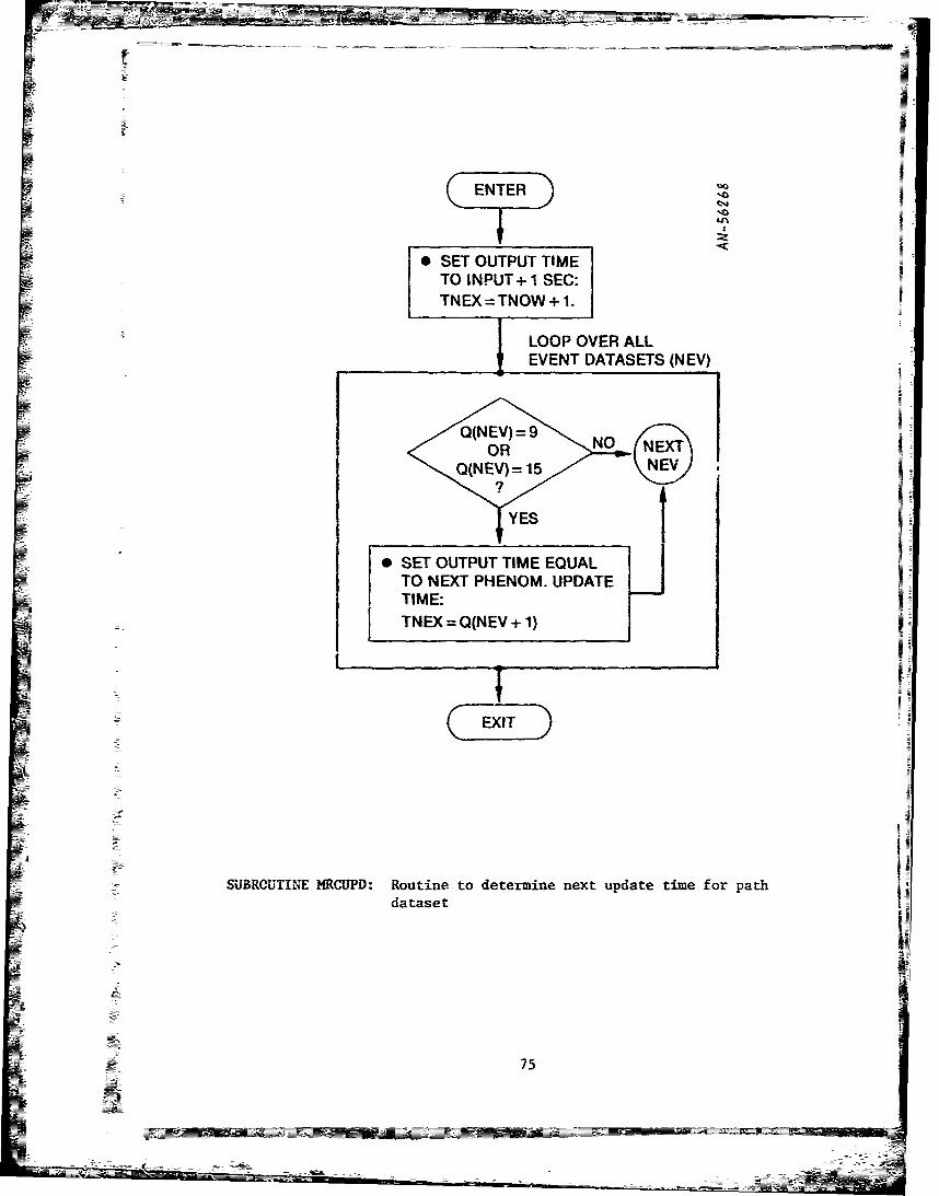
ENTER

0 SET OUTPUT TIMETO INPUT+ 1 SEC:TNEX TNOW + 1.

LOOP OVER ALLEVENT DATASETS (NEV)

Q(NEVNEV

I TEXQ(NEV+ 15

17~<4YES

1N

7ES

SSE OUTPUT TIEEQA

CENTER

*ACCESS THE PATHI DATASET (NSL) &

THE TWO TIMEDEP DATASETS,(Nil & N12)

* SET INTERNALCALC. TIMES:Ti = TIME SL(NSLjT2 = TNEX SL(NSL) I

* SET PATH DATA TIMEjTO CALL TIME:TIME SL(NSL) TNOWJ

S PRFRMTM INTERPOLATION2TOTOBRN N)DTA OR (NNl):

USN LEFR IE INTERPOLATION TO

FORMULA:TRPffTIT2, X1.X2)

=X2 -(X2 -Xl)(T2 -TNO.~VtT2 -Tl) I

* INTERPOLATE FOR POINT

KTTYiEIHl (Nil) &HOOT I I(?II)

*HERE THERE IS SPACEEXIT FOR TUMBLING TARGET

CALCULATIONS

SUBROUTINE INTRPO: Routine which is used to interpolate path data to

c urrent time

76_I

ENTER

CELL BY-CELL - NOTES I PATHS ARE ORD~ERED AS FOLLOWSEVENT -INTEGRATIONJCL ON LIST

TYPE ON T1 72

PAIH2 -... .

* Ii A AIIITGRATIO IN EIiSCAT IS DONE FORPROPERTIES jALL SANDS, SO WE SAVE XLAUI ToCALL SNELLS ITELL WHIEN TO INTEGRATE AND WREN

-0 SET KCALC I TO JUST PUT DATA AW.AYXLAM I I7 BAND

0 INITIALIZE CLOUDCOMMONS IF ARPNOPCALL CLOGEOMCALL CLOUDII

FOR EACH PATH INSLI L.------ON A LITSSLS'j

ACSTI& T2- -1 WPEOUT OF=T FOR EACH -ELiXDATASETS LIST ON PATH INS..)

~ ' CALL IRCUT r - --T--

>-~ I AT SAVO - IC~G~~ ~ EITHER r- CEATHE aFFCTS. .7 LAMASL4NELW_____ NET -CEK 1 EIISCAT AND

TIAI ~ O *CRAT - CE & RETURN SPALCXLA7 7 IZNTEGRIEI .HCELL Dt;t~K EVENTS CD THIS

0S O THE ICE~ CELLGET NEXT tO8GrES tPUI DAIA LIEW FAT I LOOPOER -t -T- IDATASET) MN.AY) CALL SPGEOt BAND INT tell APGET)

GMI2N1= eKTOT BNBI IRETURNSIGM I2I~) SGMA G4T~G' I IRRADIANCE CU)

GORY IZN1I2LA =RCOREBO(G MMS< CAIIj LL 91URAD IIICORT t2,'NI2~TMORE - ~ 1

SEED IZINI2ISEED 11mill y 0N DDpA

4 I $WTEGRTE j PATH TOTAL

GE ~ BKND SWUMA.ND SAVEj J_____

I I SULIOVER GAND xI KTOT =BKTO -

BKGD BihNBI-

I I10ZOA

I L UP TOTARGETIII SKTOT BGNBGI . KTOT

PROGRAM SPCALC: Sight path calculation event. Initializes sight pathcell list and then creates EFFECTS and EMISCAT eventsto process data cell by cell

*77

ISIETER

0 INITIAIZEPARAMETERSKPRNT =0FACT= 10.NDR=50

XDELTA = 100tNLIST=0

ro COMPUTE COSINE OFZENITH:- -

.SEPA(RDVEC SPHATITI -. IF(.a>TIr21

CSZEN = COS I.)

* CREATE THEBASIC INTEGRATIONLIST-ICALL ISPLST

0 PRINT THE CELL'LIST & THE OSA

KPN=O -" LINK WORDS.

CALL LISPRTCALL LUMP-

YES

0COMAPUTE THEATMOSPHERIC SHELLS.

INTERSECTED:CALL STEP

VOR ALL ATMSHELLSINTERSECTED'* ADD THE ATMOSP

SHELLS TO THECELL LIST*CALL INSERT

;0 PPINT THE CELLIKPRNT0 NO LIST & THE OSAIKPRNTLINK WORDS

CALL LISPATCALL LDUMP

YES

SADD THE DISTURBEDREGION CELLS.

t CALL DRCELLS

IS RIT &THE CELL

KPRNIO NO LINK WORDS.

CALLLISPRI' i

YES

SUBROUTINE SPGEOM: This subroutine creates the cell integration list

78

0 CHECK LOOK DIRECTION ANDSET UP VECTORS FORINTERSECTION CALCULATIONSSEN4SVC= RDVEC

KFLAG =0 & I=0-. SENSOR LOOKING DOWN:

KFLAG= 1a =ACOS(CSZEN)

SEPA(RDVEC, NO HBAR = RDVECP*SINa HBAR4SPHAT)SBAR = IRBODy 2 -HBART RBOOY

<TI/2H BAR>SCALE= IRDVECI-CSZEN I RBODY

+YES SENSVC = ROVEC + SCALE-SPHAT

0 SENSOR LOOKINg ',Il- OBVEC =RDVEC - SENSV^C(CONTINUE)

FO AL CHECK FOR NUC. REGION INTERSECT;ONSAFBS ON FBLIS

SCOMPUTE EXTENT (PL) OF INTERSECTION

FIREBALL 4HIHOF PATH WITH THESE REGIONS:

TYPE? L CALL EXTENT FOR FIREBALL REGION,I HA-CHEM PANCAKE.

3HLOW I ~CHEX-ION LEAK,0COMPUTE EXTENT (PLQ OF INTERSECTION DEBRIS LOSS-CONE

OPATH WITH THESE REGIONS: FOR EACH DEBRIS(ND4EXTX-. FR FIEBAL REGON 0 COMPUTE EXTENT (PL)OF INTERSECTION

CAL SHEN--R WAKEXDSALLETEN--FO~~XUSTOF PATH WITH THESE REGIONS:

____________ SHEATH, BETATUBE

CHEIUM~-- OR ILSN COUDCALL EXTENT -- FOR DEBRIS (CONTAINED),

L=?NO 0oSET F-6RAMETERS:

INDXW(I, = INDXF FB(NFB)YES KIND(I)= 10 +KINDF -(FB) 16 - CHXII.L.)

f21 -(VORTEX) 24 -(DEBRSNEXT 26 -(WAKE) 20-(SHEATH)

REGION 17 - (CHM SPHR) 19-(BETATUBE)4;~23 -(DUST) ~27 -(DEBRS L.C.) f22- (WILSON CLD) 18-(CHM PNCK)

-PUT DISTURBED REGION CELL ON LIST --CALL INSERT_

SUBROUTINE brlo.ELLS: Subroutine which creates disturbed region cells for

79

-~ -- --- -~-- -

CEKFRCLOUDSTTSIA0GE INTERSECTIONSOFLSWT

CLO12 KM ALTTUDE

0 SES) AAMTRLOOP OVER DEOTERIITC =-

C CLOT DITUBE REGINOLOU STATISTICAL ~ f

OFP INTERSECTIOIOSNF LS IT

LOO OVRE , S SET UP PARAMETERS

S0 PU T DISTURBED REGION ON SLIS CALLL INSERT

CHINERECKORLM NESCIN

SETBUPEPRARETURN

LOOP OVE N (TER

* COKFO L M UTE EX E T P)OFIERSECTION

PLUMEBALL EXTENT '1OPOTER YES O (THWTHPUME

? 0 SET PARAMETERS:

CA I= SF-.50

N E X T T A R G E T I - _ _ _ _ _ _ _ _ _ _ _

SUBROUTINE DROCELLS (continued)

80 i

FS ACCESS SENSORDATA SS CD.ST.BR.FV DATASETS

:0ACCESS FOCAL PLANEIDATASET LIST ;LIT

rF jj -ST PETFOV SIZLS FORSTORED SC.%SORMODELS

0 COMPUTE N9R& NCOF ARRAY E.FOR EACH FO1;AL PLANE ARRAY -( e

DATASET;14FA) ON ILIST

& SC(IOOAO)'FOR EACH PATH DATASET (Nil) ARRAYS PE OYP GERA E LOA

ON PLT FAIFA)FFOR ECH PAT DATASET (Nil)ONEL ON PLSTFAFA

VALPUE T AHINFCLPAE ARRAY

VALUE CTYPE- OTYPE= CALL ARRAYACKK.LL= HII(NIlI 3HF0V SHFIAEBALLS

() FOR EACH PATH (NIl) OR_____________ON PLSO FAINFA) 7HOBJECTS 0 PERFORM SENSOR

* PERFORM SENSOR] jPROCESSINGPROCESSING 6 ' SET UPSPIRE &

* SET UP SPIRE & K= RETURN OPSIM KRETURN OPSIM EVENTS I EVENTS AT TIME CLOCIAT TIME =CLOCK i ~~

I* PUT (Nil)O rNXPATH LIST S ET

NO NUMBE

~~~~~~1~~~~~~ (NEXT THSOBETON~

YETS FO NX

OTHSOBJECT NA

j*PERFORM SENSORNIEXT..4 1 N EXT J PROCESSING\NFAI. Nil 0SET UP SPIRE & RETURN

'-' IOPSIM EVENTS

PROGRAM OPSIM: Optics simulation event. Geiierates focal plane array andcalls processin60 routines

81 1

- - - - - -- la

A'0

0 GENERATEREPRESENTATION OFBACKGROUND USINGPLSG FA(NFA) LIST

FOR EACH PATH DATASET (Nil) CALL ARRAY FOR EACH PATH DATASET (Nil)ON PLSO FA(NFA) ON PLST FA(NFA)

0 K=O* ADD TARGET POINT1* PTSLS =0 INTENSITY TO

FOCAL PLANE ARRAY

CALL ARRAY

" PUT (Nil)IONPATH LIST PTSLS

DO YOU WANTTO PLOT ARRAY? NON.EXTNO K= NUMBER PLOT=7HOBJECTS NFA

PATHS OR < 0OR 3HYES!Ni THIS OBJECT

YEYES

* PRODUCE A CONTOURIII• GENERATE PLOT OF THE

REPRESENTATION OF FINAL ARRAY

THIS OBJECT IN CALL PLOTO@i ARRAY USING PTSLS

CALL ARRAY J Z i Z,I PERFORM SENSOR

PROCESSING. WIPE OUT PTSLS, SET UP SPIRE &

RETURN OPSIMEVENTS AT TIME = CLOCK

< ARRAY AFTER EACH NEXTXNFA

I "0 PRODUCE ACONTOURPLOT OF THE

ARRAY AT THIS

I POINTCALL PLOTO

PROGRAM OPSI (continued)

N; 82

r ~ _ PLOT OF THE

Gr %

FOR EACH CELL (I.J) IN ARRAY

bCOMPUTE INDICES 6HTARGET 9 ACCESS G3RID DATASETOF TARGET POINT (NGD) .COMPUTE AZM. ELV(1,J) & PUT POINT ARRAY TYPE * COMPUTE TOTAL ARRAY COORD OF CELL

A(I.J) = AMAXl(HIl (Nil), KYE ELSI W RAE(2) =FLOAT(I - (NX + IY2)I DIETOS NX &NY)DIR E C TIO N R A E (3)= F LO A T (J -(N Y + 1 M2)

*DIAM

0LOOP OVER PATH DATASETS

FOR EACH PATH DATASET (NIl)(i) ON GRID LIST ILIST

CLOSEST TO THESE CELLDIMENSIONS:RA(K) =RAE Il-,N1l)

* SET UP OTHER PATH DATA- I RE(K)= RAE Il(NI1 + 1)

NOXJ(K+l1) = G 1I(HI) XJIK) =XJ 1(NIl) -

NOo RA(K + 1) =XXX(l) K =l1.4K=ORE(K+l1) =XXX21

SIGMA(K + 1) = SIGMA Il(NIl)

CORX(K+ l)=CORX Il(NII)CE .ORY(K+ l)= CORY II(NIl) I* USE 3-0D PLANAR

NoNE

OLTO

O E

RA

" SET PARAMETERS.VALU AT THIS CELL LOCATION.P63T = AMAFP(2 VRUT PST PSAMETERX. A(I.J) = XJ 1*DY *(I - DX)

DIT MX(,+V BETPS=PSD((MAXF HMINF)) TYEDIST= AMAXI2.RC +XJ2'DX*DYTYPE + XJ3*DX*(I - DY)

H 6 LUDLM1STRUCT=2HNO + XJ40. - DX - W DXDY)IEA WHERE DX=IRAE(2)- RA(I)JDA

_____________T TUUBE______ ONr = jRAE(3)-. RE(lThDE" SET PARAMETERS I. SET PARAMETERS XJI =XJ(ll.EC

POS = P05 DC(ND)X) Pas = Bpas P = STATE(2) DE = DA t3NNGD)CLD. CLLC) 3 3*R85) TU=2NSTRUCT= 2HNO L TRUCT=3HYES I iT.E

ITIVDE'-ORRELATION.K=K 1

I =(CLOCK - TLAST)ICORTT=O. ( X TT =EXP(a) IF .4iO 1 K ETLAST =CLOCK IF T=O0

0INITIALIZE REGIONMAX & MIN DIMENSIONS(AMAX, At..N, EMAX. EMIN) &SET UP CENTER PAT H DATA- N XXJ(l)= HIl(NIl) NXRA(l) =XX-,(I)Nl

CR1XX() R Il(NIl)IRAE(l)

ISIRY GMAOR Il(NiIRl) !TIIESE COORDINATES ARE IN THEKIMl) IM lNl ROTATED FRAME (ALIGNED WITH

__________________________________________________ THE FIELD) FPCOR

SUBROTINE ARPMY: Constructs the focal plane intensity array, given pathdata describing target prints, objects, and grid s

83

AL~

0 SET UP INDICES IN FPCOR COORDINATESIFOR REGION*

NX =IFIX(AMAX - AMIN(2 xDIAM+ I)x 2+ ILNY =IFIX(EMAX -EMIN)I(2 xDIAM +I Ix 2 + I c

FOR EACH CELL (KK. LL)

IN FPCOR COORDINATES

* CONVERT TO SENSORCOORDINATES- 0 INTERF-ULATE FOR MEAN INTENSITY,

AMEAN = (XJI'FACI + XJ2"FAC2 +XJ3*FAC3JFAC4XXX()=RA(1)+FLOAT(KK-(NX+ I)Y2)*DIAM IASIGMA 0XXX(2) = RE(1) + FLOAT(LL - (NY +112PODIAMCALL FPCOR (XXX. RAE. .

STRUCT NO

CELL IN FOV. j!3HYS

/NEXTN NO RAE(2)>AZMI2 YES

CLR>L/ F INTRPOLATE FOR INTENSITY VARIATION ND

9 SPATIAL CORRELATIONS

YES ~ ASIGMA = SIG1 x FA( I +SIG2*FAC2 + SIG3*FAC3yFAC4YSACORX (CORX1 FACI + CORX2*FAC2 +CORX3*FAC3yFAC4I

DOE PAH HROGHACORY =(CORY1"FACI . CORY2'FAC2 +CORY3FAC3JFAC4 -F EXES PAT DAMICORXTHIS CELL INTERSECTH P=EXPI- DIAMIACORY)IREGION PLsi * 0-_______

CALL EXTENT _ _ _ _ _ _

ORL CLU 20OPT RANDOM SAMPLES7

P=0 IF SC(KK-.LL=OP=OIFSC(KK.LL -1)0

YSPLG-0 SIOI =SC(KK. LL - )IS01 = SC(KK -I.LL)

NO I EPS=OEPSi = (1 _ IF

2 + p

2 + T + F

2p

2T

2 -(F

2p

2 F

2T

2 *PT

2)

0LOOP OVER PATH EPS=,EPSI IF EPSI>ODATAETS(N~l ONEPS2 = (I - F

2 - p

2 +F

2p

2(I OBJECT LIST ILISTEP=PTEP2I S>OI TO FIND THREE PATHS ESESTP2I P20

CLOSESTTO THIS CELL SC(KK. LL)= -F*P*SOO+ PLS101 +F*So11XJ(KI. RA(K). REIK) + EPFSRNV(O.1)

I K13

0. COMPUTE ARRAY INTENSITY AT THIS CELL0 CALCULATE DIFFERENCES AOLD =A(I.J)

XJ1 =XJ(l) SiI = SiGMA(I) CORXI CORYi A(I.J(=AMEAN ASIGMA*SC(KK.LL) NEXTXJ2 =XJ(2) S1G2 =SIGMA(2) ( (.JAA1(OD(I)CDELLXJ3 =XJ(3) S1G3=SIGMAt3) MX(ODMA

X24 =RA(2) -XXX(1) Y41 = XXX(2) - RE(l)V23 = RE(2) - RE(3) X2i = RA(2) - RA~l)X32 = RA(3) - RA(2) Y21 = REI2) - RE(l)Y24 = RE(2) - XXX(2) FACI = X24'Y23 +X32'Y24X41 =XXXI) - RA~l) FAC2 = X41 'Y13 + X31 Y41Y13-RE~l)-RE(3) FAC3=X41*Y2 - X21IYA

IX1A3) -RA~I! FAC4=X21*Y23+X32*Y2;

84

_______ _________________

"ACCESS SENSOR DATASETS: -

OD, ST, FV, BR" ACCESS FOCAL PLANE ARRAY

AA(I.)

'S CONVERT NORMALIZED ARRAYjINTENSITIES TO RADIANCEIN (WATTS/CM 2/SR)

A(I,J) = A(I,J)*NEFDIDIAM 2

FOR ALL U, ______

* ACCOUNT FOR BLURRINGOF ARRAY DURING SCAN:

C A LL_____________________________

0GET INDEX OFNEXT TARGETON TARGETLIST(DSP PC(NEVENTS)

0 CREATE THE OUTPUTDATASET (NOM)

* ZERO THE OUTPUT ARRAYIA(I,J) =0.

0FOR EACH PROCESSING BLK0S OSPIRE LIST CALL PROPERNO

ROUTNE TO PROCESS IT:TYEXIICALL SPSUB1 = TARGETLORCALL SPSUB2

e CREATE THE TARGET MEAS.:

NETNO LAST AZMES OM(NOM) =SUMXOOTARGET 1- TARGET ELMES OM(NOM)=SUMYO

? ~RAD OM(NCM)=ARAD*NEFDETC.

YES

EXIT

PROGRAI4 SPIRE: This program calls the subroutines to scan the focal planeand process the data. Also produces ome output datasets

85

* SET UP YCOORD.I XFV02. YFV02" SET LOGICAL FLAG

FOR INSERTINGADDIT BLOCKS

MODE- OTHER HERE WE HAVE LEFT SPACE FOR

TP STORED SCANIPROCtSSING BLOCKTYPE IMODELS? GENERAL MODELS

THIS PATH FOR SCANIPROCESN 1 KF (MODEL SS(NSS) EOMODELS THAT ARE READ IN THE 1OHSURVEIL-01) CALL DATAIINPUT DECK 110HSURVEIL - 02) CALL DATA2

_ 10HSURVE!L -03) CALL DATA310HSURVEIL-04) CALL DATA4 SEi. SCN FLG 1

COMPUTE: RO SL, TH, PH &

AND SENSOR TYPE SIN(TH)DATASETS: OD, ST /_ _EXIT__ ARRX(J) = (RO + BLK(2.1)(J - 11*

I 1 ARRY(J)= YCOORD - SIGN((RO+3LK(2,1)IJ- 11)I "COS(TH,, .COORD)}

G ET SPIRE PROCESS I IO(H, COD

BLOCK LIST: CIRCULARLHV SPIRE SS(NEVENTS) J I SET SNLT ARRX(J) = BLKj3.IOUT) LINEAR SCAN SS(NS,

0 SET PARAMETERS FOR SPIRE 1 ARRY(J) BLK(4.IOUT) +SYSTEM BLOCK= I BLK(2.1)'IJ -

BLKS, = 1IBLK=1BLK(1,1)=3 -_

BLK(2.1) = DIAM ST(NST)BLK(3,1) = BLUR ST(NST) IBLK(4.1) = FLOAT (NDET ST(NST))BLK(5,1) = DNEF ST(NST)

BLK(6,1)= DNEFB ST(NST)

FOR EACH BLOCK (ND1)ON SPIRE LIST LHV

0 SET: BLKS-BLKS+, + I * READ DATA FROM SET:IBLK = IBLK + 1 O .ARRAY INTO BLKS NDET NDET ST(NST)

0 GET NUMBER OF WORDS IN ARRAY NEX BLKOT)" 2,4 1TIS BLOCK: BLK(I.IBLK)= NOI +BLK (B31) LK2V4.

IDX = IFIX (Q(NO1)) OO(NOi.I) SCS = BLURO-

NMBR=NDO(ID)FR.MB OUTFLG 2.jDX | FOR I =1.NMBR

SUBROUTINE INSENS: Initializes SPIRE scan/processing computation blocks

86

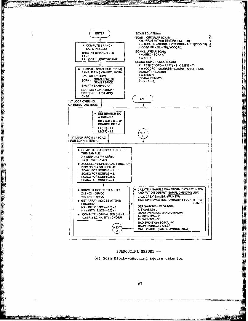
IENTER *SCAN EQUATIONS(SCANi: CInCULAR SCAN)

___X =ARRXISIN(TH) x SIN(TIPH x SL + T* COMPTE BR N~~] Y = YCOORD - SIGN(ABS(YCOORO - ARRY)JCOS(TH)

NO.PT BRIND CES x COS(TIPH x SL + TH), YCOORD)

BRI =INT (BRANCH +A) I (SCAN2: LINEAR SCAN)I X=ARRX+SCRAxTL1=1 YAR

L2=(CANLENGHISMP)(SCAN3: DSP CIRCULAR SCAN)______X = ABS(YCOORD - ARRY) x SIN) 62832 x T)I*COMPUTE SCAN RATE (SCRAIR Y =YCOORD -SIGN(ABS(Y'COORD -ARRY) xCOS

SAMPLE TIME (SAMPT), NORM. (62832-T), YCOORD)FACTOR (ONORM): I T=.62832*T

SCAN LENGTH I (SCAN4- DUMMY)SCRA = SCAN PERIOD I X=Y=T=O.

SAM PT =SAMPISCRA

DNORM = 6 28-BLUR02 .

SORT(DNEB-2SAMPT)i IDNEF

EXIT5"L- LOOP OVER NO.OF DETECTORS (NDET) rf

~~a-0SET BRANCH NO

& IN4DICES:BR= BR + (L -1)"BRANCH INTRVLLA(BR) = LiLB(BR) =L2 _ NX

"J" LOOP (FROM LI1 TO L2LFOR SCAN INTERVAL

COMPUTE SCAN POSITION FORTHIS SAMPLE:

XARRX(J) & Y = ARRY(J)

T=(JCOSMPE SCAN FUNCTIONSDEPENDING ON SCNFLG:

-0SCAN1 FOR SCNFLG = 1.SCAN2 FOR SCNFLG =2.SCAN3 FOR SCNFLG = 3.SCAN4 FOR SCNFLG= 4

F,~~~.ICONVERT COORD TO ARRAY. 0CREATE A SAMPLE WAVEFORM DATASET (NSW)

XlS = X1 + XFV02 AND PUT ON OUTPUT (SAMPL OM(NOM)) LIST:Y1S= Y1 + YFV02 I CALL CREATE(NMBR SW. NSW)

* GET ARRAY INDICES AT THIS TIME SW(NSW) = TOUT OM(NOM) + FLOATcJ - 100)*POSITION:,-. SAMPTNX = INT(X1SISCS +O05) +l DET SW(NSW) = FLOAT(BR)NY = INT(Y1StSCS, +0.5)+l K SWNSV =

*COMPUTE NORMALIZED SIGNAL=1 ADS(S~ ADO(O)IA(J,BR)=SC(NX, NY) +DNORMi AZ SW(NSW) =X1

_____________-~ EL SW(NSW)= Y1RAD SW(NSW) = SC(NX. NY)

CALL PUTBOT (SAMPL OM(NOM).NSW)

SUBROUTINE SPSUB1 -

(4) Scan Block--assuming square detector

87

ENTER

*COMPUTE BRANCH & INDICES:6= NT(BRANCH NUMBER --. 1)

Li = L.A(BR)L2 =LB(BR)X0O

"J" LOOP (FROM Li TO 1-2)FOR SCAN SAMPLES

10LOOP OVER KTO

FORM GAUSSIANRANDOM VARIABLE:X =X +RAN F(O) -. 5FOR K=1, 12

*ADD RANDOM ERRORDUE TO DETECTORNOISE TO NORM. NEXTSIGNAL:JA(J,BR)=A(J,BR)+X

EXIT

SUBROUTINE SPSUB1 -

(5) Detector Noise Block

88

ANOMUT BRANCH NUMBER. INDICES

ADSTANDARD DEVIATION FOR THISBRANCH:

BR = INT(BRANCH NUMBER)SIGMA= l.14.IBAN D PASS *SCRAISAMPLi = LA(BR)

L2 =LB(BR)Li L - INT(3-SIGMA + 1)1

ZERO THE B(J)ARRAY:B(J) =OJ =L3, L4

0PERFORM SMOOTHING FOR J =Li TO 1-2: 1J1 = J - INT(3*SIGMA + 1)J2 =J +INT(3-SIGMA +1)B(K) = B(K)+ [EXP( - (J -K)* *2/2.iSGMA *2)I

SORT (2w)ISIGMA'S(J.8R)JFOR K=Jl TO J2

* RESET THE SCAN INDICES:LA(BR) = L3LB(BR) = L4

" AND THE OUTPUT ARRAY:A(J.BR) =B(J)

FOR________ J____ =____L3______TO ______L4 ___

LOOP OVER ALL SAMPLEWAVEFORM DATASETS (NSW)

NO YES SET OUTPUT VARIABLES:NSW =T SW(NSW) J = K SW(NSW) EI

FLOAT (BR) RADS SW(NSW) =A(J.BR) - E

SUBROUTINE SPSUB2 -

(6) Gaussian Smoothing Block

-D9

SUBROUTINE SPSUBI(26) OUTPUT BLOCK - DESIGNATES SIGNALS ABOVE THRESHOLD

VALUE AS TARGETS FOR OPTION OUT2IUSED BY MODEL = SURVEIL - 02; OTHER

ENTER OPTIONS INCLUDE:OUTi TARG SW(NSW) = 9HBRIGHT PT

FOR SAMPLES ABOVE THRESHOLDOUT3 - TARG SW(NSV) = 6HDIM PT

0 OMPUTE BRANCH FOR A(K,BR) 5.6NUMBER: TARG SW(NSW) =9HBRIGHT PTBR = INT(BRANCH) FOR A(K,BR)>,3O.NUMBER) OUT4 - TARG SW(NSW) =6HBKGRND

LOOP OVER ALL & IN ADDITION CREATES TARGETWAVEFORM SAMPLE MEAS. IN SENSOR COORDINATESDATASETS (NSW) ________

NSW =FLOAT(BR)

0SET OUTPUT VARIABLES:

K =K SW(NSW)RADD SW(NSW) = A(K,BR)TARG SW(NSW) = 0.

NSXWN THRESHOLD

YES

*RESET TARGET DESIGNATIONFLAG:TARG SW(NSW) =6HTARGET

EXIT

SUBROUTINE SPSUB1 -

(26) Designates signals above threshold value as targets for option OUT2F used by MODEL.= SURVEIL-02

90

A

PROGRAM OTRACK -. THIS PROGRAM SIMULATES THE TRACKING OFAN OBJECT BY AN OPTICAL SENSOR. THESEOPTIONS ARE ALLOWED:

ENTER (iJAUTONOMOUS SENSOR TRACK - SENSORIS GIVEN SOME RANGE EST. FROMANOTHER SOURCE & TRACK IS INITIATED

-.*~A. A E AUTONOMOUSLY PIACO BR(NBR) =3HYES&

NOB. NOD, NOP. NBR. ISNET BO(IBASE) =2HNO)NSE NETTED SENSORS - SENSO,' MAY PERFORM

ACO. & MEAS. ARE NETTED(IACO = 3HYES. SNET =3HYES)

033 NETTED SENSOR NO AGO - OPTICAL SENSOR,--KTRAK TS YES CANNOT ACO (IACO =2HNO. SUET =3NYES)

< (NEVENTSi:0v

EXIT NO -!0 ACO ERtNBR >

YES4_ _ _ _ _ _ _ _ _ _ _ _

AUTONOMOUS SENSOR TRACK. 1ST LOOK SBEUN OK10GET MEAS DATASET (NOM) FOR * COMPUTE LENGTH OF TRACK FILE & SET

OBJECT CORRESP TO THIS EVENT KUTFA*PRODUCE RANGE MEAS & TAKE 1 j NWDS=A -- ONE LOOK

ELV & AZM MEAS FROM (NOM) OUT 2 NWDS a - TWO LOOKS* CONVERT TO XYZ COORO 3N WNDS = 12.- THREE LOOKS

- CAL OTRN 14 NWDS>12 -. TRACK FIL7 ESTABLISHED,e CREATE A TEMPORY TRACK FILE OF o GET MEAS. DATASET (NOM) FOR OBJECT

4 WORDS TO HOLD TIME. POSIT CORRESP. TO THIS EVENTF ~WITH DSP WORD = KDSPW 0PRODUCE RANGE MEAS. FOR KOUNT43* FIND NEXT LOOK EVENT ON EVENT OTHERWI1SE USE EST. PRANGE & GET

LIST & SET ELV & AZM MEAS.

KTRAK OLIN VNT) =KD)SPW 0CONVERT TO XYZ COORD

12ND & 3RD LOOKS <3THI MES WS=ND EXPAND TRAC.K FILE TO :NCLUDIE - KOUNT?

* FIND NEXT LOOK EVENT ON EVENT ILIST &SET - IKTRAK OL(NVNT) KTRAK TS(NEVENTS) I0SET UP SiGMAT MATRIX &SIGMA ARRAYS:

L ISIGMAT(1.1) = RERR TS(NEVENTS)-2I SIGMA(1) =SORT(S;GMAT(1.1))I SIGMAT(JJ) FXE SE(NSE + J-2)* 2

TSNE SENSE + J - 2)' NR mISIGMA(J)SOR(SIGMAT(J.Jfl

PROGRAM OTRACK, Simulates the tracking of an object by an optical sensor

91v

- ~- ~ - -~A

_

0-

< o LL~=

a: : ci:0W Dac: w '0

> a: 0I-' Cl)

002 z I.-

I >

I-- - IJY 0 u U) 02x0I i

< i-

0 w a

C.0Z) I

w ~ Z 0 .a .

3

zz co

0 .Z

0i z r-z-F. (

0

_l

0I - -E :u

z a. z 92

Cl)_ W Ii ac

DISTRIBUTION LIST

DEPARTMENT OF DEFENSE DEPARTMENT OF T14E ARmy(Cnne)

Assistant to the Secretary of Defense U .Am aelt omiAecA T T N E x c u t v e A sis a n tA T T N : D o c u m e n t C o n tro lDefense Advanced Rsch Proj Agency US ryTAO ytm nlssAtvtATTN: TIO .S AmTy TAAPyses nlsi ctvtATTN: 510, S. ZakanyczATN A-PDefense Comunications Engineer Center DEPARTMENT-OF THE Noy

AIIM: Code R410, J. M leanNaval Electronic Systems Coom nndDefense Nuclear Aciency ATTN: PE172ATTN: RAAE A :PE172ATTH: RAAE, P. Lunln Naval Itliec upr t4 cv ATTN: TITL nelgne upr tATTN: Document ControlDefenseTT eN ica nf rmtion Center Navai Ocean Systems Center12 cy AIIM (IDA T T N : C o d e 5 32Field CormandNaaPotrdteShl

Defense Nuclear Agency N aTN: Cosgrdae 1424liryATTN: FCPRATN Coe12Liry

Fiel ComondNaval Research LaboratoryDefense Nuclear Agency ATTN: Code 467, .BrnLivermore Branch -ATTN: Code 4700, J. CrofeATTN: FCPRL ATTN: Cd 70 .Cfe

AT:Code 4780, 5. OssakowNatinal ecurty AencyATTN: Cod? 4780, P. PalmadessoN ATN ScRity, Agency maATNATT: -5, 3.SkllanAIM:Code 4709, W. AliUndesecetay ofDefforRsch& EqrgNaval Surface Weapons Center

ATTN: Strategi c & Space Sys '(OS)ATN CoeX1WWICS Sste EngneeingOrgNaval~ Surface Weapons CenterI IR .C S y t m E n er i ngfo rgA C o d e F -1 4 , R . B u t l e r

DEPARTMENT OF HE ARMY SrtgcSsesPoetOfcAtmospheric Sciences Laboratory ATTN: NSP-2722, F. WimberlyU.S. Army Electronics R&D Comand ATTNJ: USSP-2722, M . MeseroleATTN: DELAS-ED, F. iles DEPARTMENT OF THEAR FORCEBHD Advanced Technology CenterAiFocGopycs

abrtyDepartment of the Ar' ATir Fo PRe A.pysc SaoratrATTN: ATC-T, M. Capps ATTN: OPR, H. StarirATTN: ATC-o, w: Davies ATTN: SULL .Gadie8140 Systems Coriand ATTN: LKB, K. ChampionDepartment of the ArmyATTN: BMDSC-HiW, R. Dekalb Air Force Systems CoymmandHarry Diamond Laboratories

ArFreTcnclAp ctosCneDepartment of the Army Air Iorc Technical AplibarynCneATTN: DEI.HD-I-I'LATN TehiaLbryATTN: DELRD-h-P, F. Wimenitz hTTN: TFR, C. Meneely-i

Air Force Weapons LaboratoryU.S. Army Foreign Science & Tech Ctr ArFreSsesCninATTN: DRXST-SD ATrIorc SULemsCmmnU.S. Army missile Intelligence Agency ATTN: DYC

ATTN: J. Gambtle Ballistic Missile OfficeU.S. Army Missile R&D Comand Air Force Systems Command

ATTN DRDI-XSATTN: MMxATTNJ: RMI- ATTN: MNRCATTN: RSICATTN: M NRTE('.5. Army Nuclear & Chemical Aqency

ATTH: Library

93

Er_ _ __ _

I

a

DEPARTMENT OF THE AIR FORCE (Continued) DEPARTMENT OF DEFENSE CONTRACTORS (Continued)

Deputy Chief of Staff General Research CorpResearch, Development, & Acq ATIN: J. Ise, JrDepartment of the Air Force ATTN: J. Garbarino

ATTN: AFRDSJamieson Science & Engineering

Headquarters Space Division ATTN: J. JamiesonAir Force Systems Command

ATTN: SKX Kaman Sciences CorpATTN: SKA, M. Clavin ATT:i: N. Beauchamp

ATTN: D. PerioHeadquarters Space Division ATTN: P. TracyAir Force Systems Command

ATTN: SZJ, P. Kelley Lockheed Missiles & Space Co, IncATTN: D. Divis

Rome Air Development CenterAir Force Systems Command Lockheed Missiles & Space Co, Inc

ATTN: OCS, V. Coyne ATTN: M. WaltATTN: TSLDATTN:. OCSA, J. Simmons M.I.T. Lincoln Lab

ATTN: D. TowleStrategic Air CommandDepartment of the Air Force IcDonnell Douglas Corp

ATTN: NRT ATTN: R. HalprinATTN: XPFS, B. Stephan ATTN: H. Spitzer

DEPARTMENT OF ENERGY Mission Research CorpATTN: D. Archer

Department of Energy ATTN: D. SkppenfieldATTI: OMA ATTN: F. Fajen

ATTN: R. HendrickOTHER GOVERNMENT AGENCIES ATTH: R. Bogusch

ATTN: M. Scheibe

Department of Commerce ATTN: R. KilbNational Oceanic & Atmospheric Admin

ATTN: F. Fehsenfeld Nichols Research CorpATTN: N. Byrn

Institute for Telecommunications Sciences TATTN: G. Falcon Pacific-Sierra ResearchATTN: W. Utlaut ATTN: H. Brode

DEPARTMENT OF DEFENSE CONTRACTORS Photometrics, Inc

Aerojet Electro-Systems Co ATTN: I. Kofsky

ATTN: J. Graham Physical Research, Inc

Aerospace Corp ATTN: R. Deliberis

ATTN: J. Reinheimer University of PittsburghATTN: I. Garfunkel ATTN: F. KaufmanATTN: N. StockwellATTN: V. Josephson R & D AssociatesATTN: N. Cohen ATTN: R. LelevierATTN: J. Stiauss

ATTN: F. Gilmore

ATTN: P. HaasBerkeley Research Associates, Inc ATTN: B. Gabbari

ATTN: J. Workman ATTN: R. Turco

ESL, IncESL, IcR D Associates

ATTN: J. Marshall A t .ATTN: B. Yoon

General Electric Co Rand CorpATTN: M. Bortner ATTN: C. Cram

General Electric Company-TEMPO Science Applications, IncATTN: T. Stephans ATTN: D. HamlinATTN: J. JordanoATTN: DASIAC Science Applications, IncATTN;: M. Stanton ATTN: W. MendesATTN: W. Knapp

94!Ae

Ri

DEPARTMENT OF DEFENSE CONTRACTORS (Continued) DEPARTMENT OF DEFENSE CONTRACTORS (Continued)

SRI International Visidyne, IncATTN: W. Chesnut ATTN: C. HumphreyATTN: W. Jaye ATTN: J. Carpenter

ATTN: H. SmithTeledyne Brown Engineering

ATTN: Technical LibraryATTN: G. Harney

ATTN: J. Cato

95

96